Embed Size (px)
Citation preview

UNIVERSITY OF CALGARY
Real Time Torque and Drag Analysis during Directional Drilling
by
Mohammad Fazaelizadeh
A THESIS
SUBMITTED TO FACUALTY OF GRADUATE STUDIES
IN PARTIAL FULFILMENT OF THE REQUIREMENTS FOR THE
DEGREE OF DOCTOR OF PHILOSOPHY
DEPARTMENT OF CHEMICAL AND PETROLEUM ENGINEERING
CALGARY, ALBERTA
March, 2013
© Mohammad Fazaelizadeh 2013

ii
Abstract
The oil industry is generally producing oil and gas using the most cost-effective solutions.
Directional drilling technology plays an important role especially because the horizontal wells
have increased oil production more than twofold during recent years.
The wellbore friction, torque and drag, between drill string and the wellbore wall is the most
critical issue which limits the drilling industry to go beyond a certain measured depth. Surface
torque is defined as the moment required rotating the entire drill string and the bit on the bottom
of the hole. This moment is used to overcome the rotational friction against the wellbore, viscous
force between pipe string and drilling fluid as well as bit torque. Also, the drag is the parasitic
force acting against drill string movement to pull or lower the drill string through the hole. The
drill string friction modeling is considered an important assessment to aid real time drilling
analysis for mitigating drilling troubles such as tight holes, poor hole conditions, onset of pipe
sticking, etc. In directional drilling operations, the surface measurement of weight on bit and
torque differs from downhole bit measurement due to friction between the drill string and
wellbore. This difference between surface and downhole measurements can be used to compute
rotating and sliding friction coefficients from torque and hook load values respectively. These
friction coefficients are used as indicators for real time drilling analysis.
To do this analysis, analytical and finite element approaches were used to develop practical
models for torque and drag calculations for any well geometry. The reason why two different
approaches were used to develop torque and drag models is that the drill string was assumed to
be soft string in the analytical approach which has full contact with the wellbore. In the finite
element approach, the effect of drill string stiffness was included in the model and the drill string
does not have full contact with the wellbore. Also, a new method for effective weight on the bit
estimation was developed using wellbore friction model. The new method only utilizes the
available surface measurements such as hook load, stand pipe pressure and surface rotation.
Using the new method will eliminate the cost of downhole measurements tools and increase
drilling rate of penetration by applying sufficient weight on the bit.
In this research, different effects which have great contributions on torque and drag values were
investigated precisely. These effects include buoyancy, contact surface due to curve surface area,

iii
hydrodynamic viscous force, buckling, hydraulic vibrations, adjusted unit weight and sheave
efficiency.
Finally, some field examples from offshore and onshore wells were selected for model validation
and verification. The field data include hook load and surface torque for different operations
such as drilling, tripping in/out and reaming/back reaming.

iv
Acknowledgments
I would like to express my appreciation to Dr. Geir Hareland for his supervision, advice, and
guidance from the beginning of my study as well as giving me valuable experiences all the way
through my research work, with his endurance and knowledge, while allowing me the
opportunity to work independently.
I wish to thank Dr. Bernt Aadnoy, University of Stavanger, and Dr. Zebing (Andrew) Wu,
University of Calgary, for their help and contributions during the development of analytical and
finite element method modeling.
My gratitude also extends to Dr. Raj Mehta, Dr. Gordon Moore, Dr. Larry Lines and Dr. Mesfin
Belayeneh for serving on my examination committee.
I would thank Dr. Mazeda Tahmeen and Mohammad Moshirpour for programming and software
development as well as Benyamin Yadali and Patricia Teicheob for editing and proofreading of
my thesis.
I am really thankful of Department of Chemical and Petroleum Engineering, University of
Calgary for the giving me the chance to pursue my studies in the Doctor of Philosophy program.
Finally, I would like to thank my family, particularly my wife, Mahdieh Salmasi, for their
constant support and inspiration throughout my entire studies.

v
Table of Contents
Abstract ...................................................................................................................................................................... ii
Acknowledgments ................................................................................................................................................. iv
Table of Contents .................................................................................................................................................... v
List of Tables........................................................................................................................................................ viii
List of Figures ......................................................................................................................................................... ix
Nomenclature ......................................................................................................................................................... xii
CHAPTER ONE: INTRODUCTION ............................................................................................................... 1
CHAPTER TWO: LITERATURE REVIEW ................................................................................................. 5
2.1 Analytical Modeling ............................................................................................................. 5
2.2 Finite Element Modeling .................................................................................................... 13
CHAPTER THREE: TECHNICAL APPROACH – ANALYTICAL ................................................. 18
3.1 Buoyancy Factor ................................................................................................................. 18
3.2 Straight Sections Modeling ................................................................................................. 19
3.3 Curved Sections Modeling .................................................................................................. 23
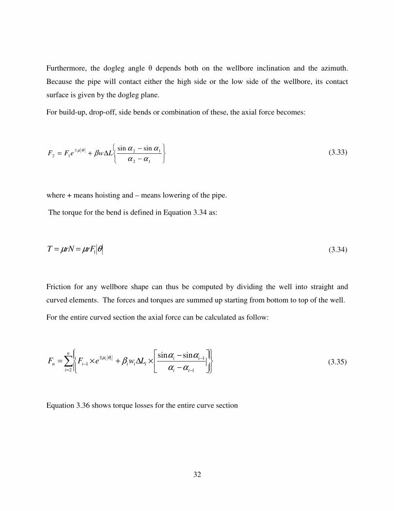
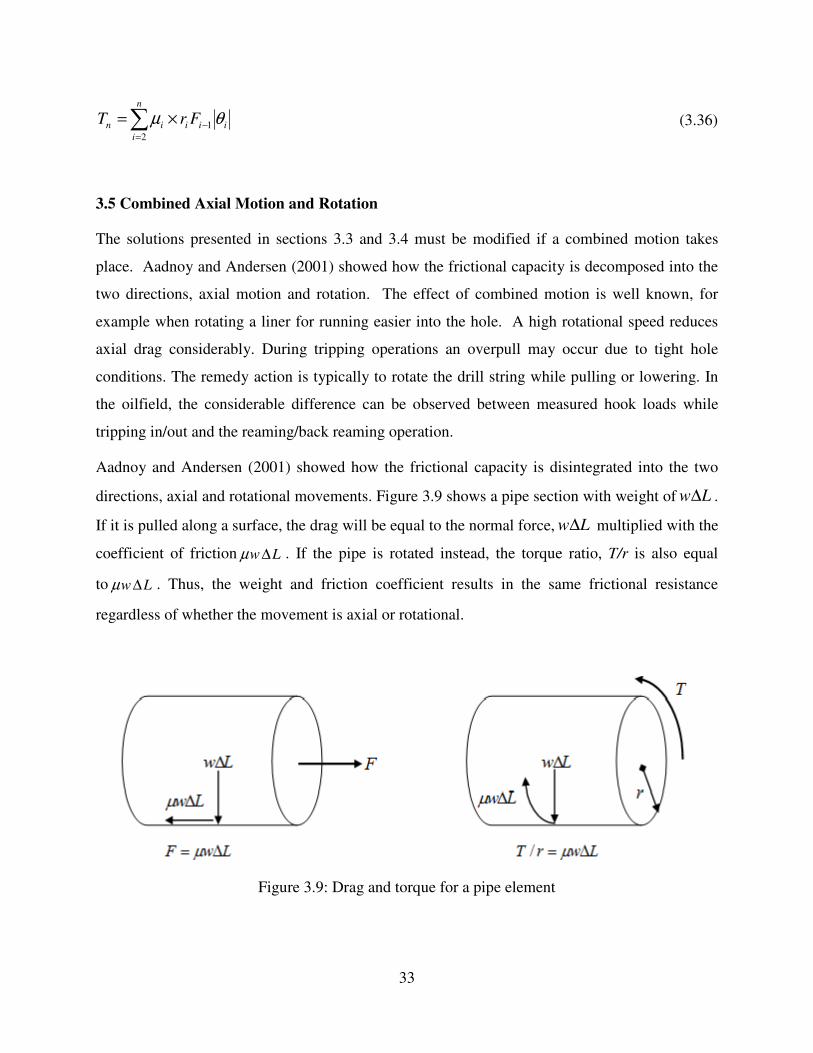
3.5 Combined Axial Motion and Rotation ................................................................................ 33
3.5 Application of the New Model ........................................................................................... 38
3.5.1 Case A: Analysis of a Two Dimensional S-shaped Well ............................................. 38
3.5.2 Case B: Analysis of a 3-dimensional Well .................................................................. 45
3.5.3 Case C: Combined Motion in 3-dimensional Well ..................................................... 46
CHAPTER FOUR: TECHNICAL APPROACH- FINITE ELEMENT .............................................. 49
4.1 Hamilton’s Principle ........................................................................................................... 50
4.2 Shape Function.................................................................................................................... 50
4.3 The Dynamic Equations ...................................................................................................... 51
4.4 The Mass Matrix ................................................................................................................. 52
4.5 The Stiffness Matrix ........................................................................................................... 54
4.6 The Damping Matrix........................................................................................................... 57
4.7 Force Vector........................................................................................................................ 58
4.8 Transform Matrix ................................................................................................................ 60
4.9 Global Matrix ...................................................................................................................... 62
4.10 Boundary Conditions ........................................................................................................ 63
4.11 Solution Method................................................................................................................ 67
4.11.1 Houbolt Method ......................................................................................................... 68

vi
4.11.2 Newmark Beta Method ............................................................................................... 69
4.11.3 Park Stiffly Stable Method ......................................................................................... 70
4.11.4 Wilson Theta Method ................................................................................................. 71
4.12 Torque and Drag Modeling ............................................................................................... 73
CHAPTER FIVE: MODELING CONSIDERATIONS ........................................................................... 81
5.1 Buoyancy ............................................................................................................................ 81
5.1.1 Underbalanced Drilling ............................................................................................... 82
5.2 Viscous Drag Force............................................................................................................. 86
5.3 Contact Surface ................................................................................................................... 89
5.4 Sheave Friction ................................................................................................................... 91
5.5 Hydraulic Vibrations ........................................................................................................... 93
5.5.1 Agitator ........................................................................................................................ 94
5.5.2 Surface Pressure Applied inside Drill string ............................................................... 97
5.6 Buckling .............................................................................................................................. 98
5.6.1 Buckling Criteria ......................................................................................................... 98
5.6.2 Axial Force along Drill string .................................................................................. 100
5.7 Off/On Bottom Data Selection.......................................................................................... 102
5.8 Adjusted Unit Weight ....................................................................................................... 103
CHAPTER SIX: TECHNICAL RESULTS AND DISCUSSION ................................................... 106
6.1 Analytical Modeling of a Two-Dimensional Well ........................................................... 106
6.1 .1 Tripping Out.............................................................................................................. 108
6.1.2 Tripping In ................................................................................................................. 112
6.1.3 Reaming/ Back Reaming ............................................................................................ 114
6.1.4 Effect of Contact Surface ........................................................................................... 118
6.1.5 Effect of Hydrodynamic Viscous Force ..................................................................... 120
6.2 Three Dimensional Well-Analytical Modeling ................................................................ 123
6.2.1 Tripping out ............................................................................................................... 124
6.2.2 Tripping In ................................................................................................................. 127
6.3 Detection of Drill string Sticking - Analytical Modeling ................................................. 133
6.4 Three Dimensional Well-Finite Element Modeling ......................................................... 141
6.5 Estimation of Downhole WOB and Bit Torque ................................................................ 147
6.5.1 Background ................................................................................................................ 148
6.5.2 Vertical Well .............................................................................................................. 151
6.5.3 Extended Reach Well ................................................................................................. 154

vii
6.5.4 Horizontal Well .......................................................................................................... 156
6.5.5 Description of System ................................................................................................ 158
6.5.6 Example Application .................................................................................................. 162
6.5.7 Field Application ....................................................................................................... 170
CHAPTER SEVEN: CONCLUSIONS AND RECOMMENDATIONS .......................................... 176
References ............................................................................................................................................................ 179

viii
List of Tables
Table 3.1: Forces in the drill string during hoisting and lowering............................................... 41
Table 3.2: Torque in drill string during drilling while bit is off bottom ...................................... 42
Table 4.1: Comparison of Exact value with FEA of the rod ........................................................ 78
Table 5.1: The multipliers for various classes of pipes (Samuel, 2010) ..................................... 104
Table 6.1: Flow regimes for different drill string position at different tripping speed ............... 122

ix
List of Figures
Figure 1.1: Schematic of directional drilling (Discovery Channel Online, 2011) .......................... 1
Figure 1.2: Measurement While Drilling (Soft online, 2011) ........................................................ 3
Figure 2.1: Schematic of bottom hole assembly (BHA) (Yang, 2008) ........................................ 14
Figure 2.2: Reference and local coordinate systems (Yang, 2008) .............................................. 15
Figure 2.3: Three dimensional finite beam element (Schmalhorst and Neubert, 2003) ............... 16
Figure 2.4: Boundary conditions (Bueno and Morooka, 1995) .................................................... 16
Figure 3.1: Force balance for pipe pulling along a straight surface............................................. 20
Figure 3.2: Geometry of the inclined straight pipe ...................................................................... 21
Figure 3.3: Definition of change in direction θ over a length ∆L ................................................. 23
Figure 3.4: The unit vector e is decomposed along the x-axis, the y-axis, and the z-axis (vertical)....................................................................................................................................................... 24
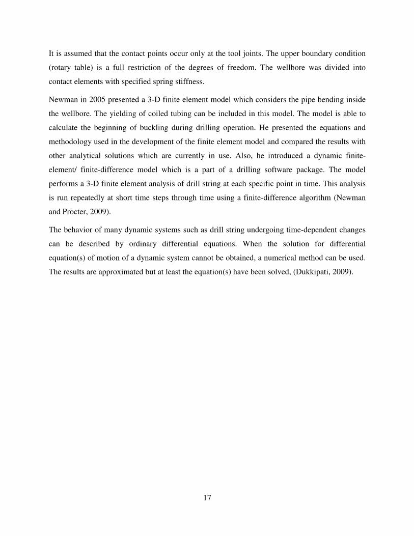
Figure 3.5: The dogleg in 3-dimensional space ............................................................................ 26
Figure 3.6: Projection of a wellbore in a vertical plane ................................................................ 27
Figure 3.7: Projection of wellbore in a horizontal plane. In this projection the wellbore is assumed to be circular. .................................................................................................................. 28
Figure 3.8: Element pulled along curved surface ........................................................................ 31
Figure 3.9: Drag and torque for a pipe element ............................................................................ 33
Figure 3.10: Relationship between hoisting/lowering and rotational speed ................................ 34
Figure 3.11: Relationships between torque and drag for straight pipe sections .......................... 35
Figure 3.12: Relationship between torque and drag for bend ....................................................... 37
Figure 3.13: Geometry of S-shaped well ..................................................................................... 40
Figure 3.14: Torque and drag for the S-shaped well ................................................................... 43
Figure 3.15: Torque along drill string during off/on bottom conditions...................................... 44
Figure 3.16: 3-dimensional well shape ........................................................................................ 45
Figure 3.17: Wellbore friction for 3-dimensional well ................................................................ 46
Figure 3.18: Comparison between pure hoisting/lowering and combined motion ...................... 47
Figure 3.19: Torque along drill string with combined motion..................................................... 48
Figure 4.1: Generalized displacement for a beam element ........................................................... 51
Figure 4.2: Distributed forces due to gravity on an inclined element ........................................... 59
Figure 4.3: The forces applied on an element of drill string ......................................................... 59
Figure 4.4: Difference between element local coordinate system and global coordinate system 61
Figure 4.5: Main boundaries on the drill string in the wellbore ................................................... 64
Figure 4.6: Constraint relations between drill string and wellbore .............................................. 67
Figure 4.7: Cubic curve pass through four ordinates .................................................................... 68
Figure 4.8: Linear changes of accelerations for a dynamic system .............................................. 71
Figure 4.9: The interaction between drill string and wellbore ...................................................... 74
Figure 4.10: Flow chart of the FEA program for torque and drag analysis .................................. 76
Figure 4.11: FEA of a rod with one end fixed .............................................................................. 78
Figure 4.12: FEA of vertical well drilling .................................................................................... 79
Figure 4.13: The axial displacement of four different locations ................................................... 80
Figure 4.14: The rotary speed at three different locations ............................................................ 80
Figure 5.1: Effect of hydraulic vibration on axial friction force (Agitator Tool Handbook, 2008)....................................................................................................................................................... 94

x
Figure 5.2: The tension-compression and axial friction forces along drill string without agitator (Agitator Tool Handbook, 2008) .................................................................................................. 95
Figure 5.3: The tension-compression and axial friction forces along drill string using agitator (Agitator Tool Handbook, 2008) .................................................................................................. 96
Figure 5.4: Effect of using agitator on drilling parameters (Agitator Tool Handbook, 2008) ..... 97
Figure 5.5: Schematic of tubular buckling in horizontal section ................................................ 101
Figure 5.6: Selection of off bottom data using stand pipe pressure ............................................ 103
Figure 6.1: Geometry of the horizontal well in Alberta, Canada................................................ 106
Figure 6.2: Drill string configuration for the horizontal well ..................................................... 107
Figure 6.3: Measured hook load versus measured depth during tripping out ............................. 108
Figure 6.4: Comparison between the measured and calculated hook loads during tripping out 109
Figure 6.5: Comparison between the measured hook load and the static weight of the drill string during tripping out ...................................................................................................................... 110
Figure 6.6: Comparison between the corrected field data and modeling results for tripping out111
Figure 6.7: Comparison between two subsequent measured hook loads during tripping out .... 112
Figure 6.8: Comparison between measured and calculated hook loads while tripping in .......... 113
Figure 6.9: Sensitivity analysis of friction coefficient vs. measured depth while tripping in .... 114
Figure 6.10: Comparison between the measured and calculated surface torque during reaming and back reaming ........................................................................................................................ 115
Figure 6.11: Effect of pipe rotation on the calculated hook load during tripping in/out ............ 116
Figure 6.12: Effect of tripping speed on the calculated torque during reaming operation ......... 117
Figure 6.13: Effect of pipe rotation on the calculated torque values during reaming operation 118
Figure 6.14: Effect of contact surface on the calculated drag values during tripping in/out ...... 119
Figure 6.15: Effect of contact surface on the calculated torque values during tripping in/out ... 120
Figure 6.16: Effect of mud rheology and clearance on the hydrodynamic viscous drag force .. 121
Figure 6.17: Effect of tripping speed and flow regime on hydrodynamic viscous drag force ... 122
Figure 6.18: Well geometry with casing shoe depths ................................................................. 123
Figure 6.19: Comparison between the field and models hook load data using friction coefficient of 0.2 during tripping out ............................................................................................................ 125
Figure 6.20: The tripping out procedure for North Sea candidate well in terms of flow rate and drill string rotation ...................................................................................................................... 126
Figure 6.21: Comparison between the field and models torque data using a friction coefficient of 0.2 for tripping-out ...................................................................................................................... 127
Figure 6.22: Buoyancy factor profile during tripping-in ............................................................ 128
Figure 6.23: Comparison between the field and models hook load data using a friction coefficient of 0.2 for tripping in .................................................................................................................... 129
Figure 6.24: Friction coefficient versus the measured depth during tripping in and out ............ 130
Figure 6.25: The tripping in procedure in terms of flow rate and drill string rotation ............... 131
Figure 6.26: Comparison between the field and models torque data using a friction coefficient of 0.2 during tripping in .................................................................................................................. 132
Figure 6.27: Well geometry of stuck well .................................................................................. 133
Figure 6.28: Illustration of BHA-tight hole effect on the friction coefficient ............................ 134
Figure 6.29: Buoyancy factor profile during different operations .............................................. 135
Figure 6.30: Mud pressure gradient versus measured depth during drilling operation .............. 136
Figure 6.31: Hook load data versus measured depth during tripping in and out ........................ 137
Figure 6.32: Friction force versus measured depth during tripping out ..................................... 138

xi
Figure 6.33: Overall friction coefficient versus measured depth during tripping out ................ 139
Figure 6.34: Friction force versus the measured depth during tripping in.................................. 140
Figure 6.35: Overall friction coefficient versus measured depth during tripping in .................. 141
Figure 6.36: Comparison between the field and finite element hook load data using a friction coefficient of 0.2 during tripping out .......................................................................................... 142
Figure 6.37: Comparison between the field and finite element hook load data using friction coefficient of 0.2 during tripping in ............................................................................................ 143
Figure 6.38: The calculated torque versus measured depth ........................................................ 144
Figure 6.39: Geometry of a drilled well including vertical, build-up, straight inclined and horizontal sections ...................................................................................................................... 145
Figure 6.40: Comparison between hook load data of field and finite element modeling data during drilling ............................................................................................................................. 146
Figure 6.41: Comparison between analytical and finite element modeling result with field tripping out data .......................................................................................................................... 147
Figure 6.42: Schematic illustration of drilling rig that shows the auto driller system is connected to deadline to estimate downhole weight on the bit .................................................................... 149
Figure 6.43: Schematic description of drill string moving downwardly in a vertical well while the bit is off and on bottom, respectively.......................................................................................... 152
Figure 6.44: Schematic of drill string moving downwardly in a well with the geometry of vertical, build-up and the straight inclined sections .................................................................... 154
Figure 6.45: The drill string along a horizontal well which is pushing toward the bottom ........ 157
Figure 6.46: The flowchart showing the steps for calculating downhole weight on the bit using the hook load measurements ....................................................................................................... 159
Figure 6.47: The flowchart showing the steps for the calculation of downhole bit torque by using the surface torque measurements ................................................................................................ 162
Figure 6.48: Comparison between tension and compression along drill string when 11kdan weight is applied on the bit ......................................................................................................... 165
Figure 6.49 shows reduction in axial friction force along drill string when 11 kdaN weight is applied on the bit. ........................................................................................................................ 166
Figure 6.50 Comparison between surface and downhole weight on the bit for 1m drilled interval..................................................................................................................................................... 168
Figure 6.51: shows the surface and downhole bit torque for 1m drilled interval ....................... 170
Figure 6.52: Geometry of a short bend horizontal well including vertical, build-up and horizontal sections ........................................................................................................................................ 171
Figure 6.53: Plot of friction coefficient versus measured depth during drilling operation for the interval between 3070 m to 3420 m ............................................................................................ 172
Figure 6.54: Comparison between surface and downhole WOBs for the drilled interval between 3070 m to 3420 m. ...................................................................................................................... 173
Figure 6.55: Plot of surface WOB values versus measured depth during drilling operation when keeping 10 kdaN downhole weight on the bit ............................................................................ 174
Figure 6.56: Comparison between surface and downhole weight on the bits using K value for a drilled interval from 2534m to 2538m ........................................................................................ 175
xii
Nomenclature
α Inclination angle (rad)
β buoyancy factor
γ Specific weight (N/m3)
η contact surface angle(rad)
δ pipe-wellbore ratio
ε rotational displacement (m)
θ dogleg angle(rad)
µ friction coefficient
υ Poisson’s ratio
ρ density,(kg/m3)
φ azimuth angle (rad)
ψ angle between axial and tangential pipe velocities (rad)
Ω rotary speed, (1/sec)
∆d clearance between wellbore and drill string (m)
∆L length of an element (m)
A cross sectional area of drill string (m2)
BHA bottom hole assembly
Cc mud clinging constant
Cs contact surface correction factor
d drill string outer diameter(m)
D wellbore diameter(m)

xiii
DL dogleg angle(rad)
DLS dogleg severity(rad/30m)
DWOB downhole weight on the bit (N)
e sheave efficiency
E modulus of elasticity (N/m2)
F axial load along drill string(N)
FD hydrodynamic viscous drag force(N)
FN normal force (N)
Fdl deadline tension (N)
FF friction force(N)
F generalized nodal force vector
G shear modulus (Pa)
gn gravity acceleration (9.8066 m/sec2)
HL hook load (N)
i number of element
I area moment of inertia (m4)
J polar moment of inertia (m4)
k kinetic energy (J)
[K] system stiffness matrix
L length (m)
m& mass flow rate (kg/min)
[M] system mass matrix
n flow behavior index
N number of drilling lines

xiv
Nr rotary speed (rpm)
NRe Reynolds’s number
p potential energy (N.m)
P pressure (N/m2)
Pg absolute atmospheric pressure (N/m2)
PV plastic viscosity (cp)
Q volumetric flow rate (m3/min)
r radius of tool joint (m)
R radius of curvature (m)
Rα radius of bend in vertical plane (m)
Rφ radius of bend in horizontal plane (m)
ROP rate of penetration m/sec
S specific gravity
SWOB surface weight on the bit (N)
t pipe wall thickness (m)
T torque in string (N.m)
Tave absolute average temperature (K)
Tg absolute atmospheric temperature (K)
U displacement (m)
u& velocity (m/sec)
u&& acceleration (m/sec2)
u displacement vector
U generalized nodal displacement vector
V resultant velocity (m/sec)

xv
vae average effective velocity (m/sec)
vh hoisting velocity (m/sec)
vp pipe velocity (m/sec)
vr rotational velocity (m/sec)
w unit weight of drill string (N/m)
W static weight of drill string (N)
Subscripts
1 bottom of element
2 top of element
g gas
l liquid
m mud
mix mixture
w water
x, y, z components in x, y and z directions

1
CHAPTER ONE: INTRODUCTION
“People outside the oil and gas industry believe that most oil and gas wells are drilled vertically,
in a simple straight line. In reality, most oil and gas well profiles can be anything but straight
vertical. Some of them are actually tangent from the vertical and then depart in a different
direction. These wells are called directional wells. The primary purpose of a directional well is to
reach oil or gas targets that are underneath places that are difficult to reach such as a city or a
lake as well as oil companies even drill deviated wells in order to reach several targets”,
Discovery Channel Online, (2011).
Figure 1.1: Schematic of directional drilling (Discovery Channel Online, 2011)
One of the advantages of directional drilling is that it provides a larger producing interval length
by drilling through the reservoir at an angle. It means the larger the angles in the reservoir, the
more oil and/or gas can be produced through the one wellbore. Currently, the most drilled type of
directional well is the horizontal well which develops into an inclination angle around 90° from
vertical. As the hydrocarbon stores horizontally in some suitable formations, it becomes
interesting for the oil and gas companies to drill their oil and gas wells horizontally.
2
Directional drillers are given a well path by the well planner and geologist. Periodic surveys are
taken while drilling to provide inclination and azimuth of the wellbore. This is typically taken
between every 30 and 500 ft and most commonly every 90 ft. If the current path deviates from
the planned path, corrections could be made by different available techniques. If the deviation is
not that severe, the well path can be corrected by changing rotational speed as well as drill string
weight and stiffness. For severe cases, introducing new downhole motor with a bent sub is the
solution that is more complicated and time consuming (KFUPM online, 2011).
Two important tools are used for directional drilling. The first is the mud motor which is
positioned exactly above the drill bit at the end of the drill string. The mud motor not only
generates additional power through the drilling hydraulic to the bit while drilling, it can bend and
turn the well in different directions. The second one is the Measurement While Drilling (MWD)
which is used for constant reporting on well path changes through the use of mud impulses from
down hole to surface. The MWD service will be added to update survey measurements to use for
real time adjustment. Accelerometers and magnetometers measure inclination and azimuth
(Halliburton Online, 2011). MWD is expensive and is not always used. Instead of MWD, the
wells are surveyed after drilling through the formations and the a multi-shot surveying tools run
into drill string on a wireline to measure inclination and azimuth angle at the different measured
depths.
With a MWD tools, the drilling crew can guide the well toward the planned target as well as
receiving the following downhole information while drilling.
rpm at the bit
smoothness of that rotation
type and severity of any downhole vibrations
downhole temperature
bit torque and weight on the bit
mud flow volume
The measured downhole parameters are transmitted from downhole to the surface using mud
pulse telemetry. The mud pulse telemetry can be divided into three general categories: positive

3
pulse, negative pulse and continuous wave. The positive pulse tools work by briefly restricting
the mud flow within the drill string which causes a raise in surface pressure. The negative pulse
tools operate by briefly venting drilling fluid from inside of the drill string out to the annulus
which causes a pressure drop that can be seen at the standpipe pressure at the surface. Finally,
continuous wave tools generate the sinusoidal wave through the mud within the drill string
(KFUPM online, 2011).
Figure 1.2: Measurement While Drilling (Soft online, 2011)
In the past decades, the reach of directional and horizontal wells has increased. Because of this
evolution in directional drilling the numbers of offshore platforms to drain offshore oilfields
have been significantly reduced which allows more wellheads to be grouped together on one
surface location.

4
The friction between drill string and the wellbore which is known as torque and drag is one of
the critical limitations which not allow the drilling industry to go beyond a certain measured
depth. In deviated well construction, it is vital to monitor torque and drag to make sure they are
in normal “acceptable” range. For this reason, the torque and drag modelling is regarded as an
invaluable process to mitigate drilling problems in different stages of directional drilling. Torque
and drag analysis has proven to be useful in well planning/design, real time analysis and post-
analysis.
During the well planning phase the wellbore friction analysis is used to optimize the trajectory
design to minimize the torque, drag and contact forces between the drill string and the borehole
wall. In real time analysis, used together with monitoring of wellbore conditions during different
operations, torque and drag modeling is particularly useful in diagnosing hole cleaning problems,
impending differential sticking, and severe doglegs as well as determining the possibility of
reciprocating casing during cementing operations. In post analysis the wellbore friction modeling
helps to analyze true causes of wellbore problems that previously were unexplained or attributed
to other factors such as mud weight, mud chemistry or problems related to sensitive shale
formations.

5
CHAPTER TWO: LITERATURE REVIEW
To ascertain a background for this research, a study is completed in this chapter about the most
important researches and studies in the area of torque and drag modeling and analysis. This
chapter is divided into two different parts; one for the analytical approach which is based on the
soft string theory and another is the finite element method which considers drill string stiffness in
the calculations.
2.1 Analytical Modeling
In the analytical modeling the drill string is assumed to be like a cable and forces due to bending
moments have not been considered to affect the normal forces as well as friction force between
the drill string and the wellbore. This is fairly good assumption as it may contribute little normal
forces on the overall force balance. In reality, the friction coefficient is not really a single
coefficient; it is an overall factor that considers all the other different friction factors. These
factors include mud system lubricity, cuttings bed, key seats, stabilizer and centralizer
interaction, differential sticking, dogleg severity, hydraulic piston effect and viscous force.
For torque and drag calculation modeling, an element of the drill string is considered in the
wellbore which is filled with drilling fluid. The forces acting on the pipe element are buoyed
weight, axial tension, friction force and normal force perpendicular to the contact surface of the
wellbore. Calculation of the normal force is the first step in calculating the friction force for an
element of the drill string. The friction force is defined as an acting force against pipe movement
which is equal to friction coefficient multiplied by the normal force as shown in Equation 2.1
NFFF ×= µ (2.1)
where
FF: friction force, N

6
µ: friction coefficient
FN: normal force, N
In straight inclined and horizontal sections, the normal force is equal to the normal weight of the
element and there is no other contribution, but for a curved section such as build-up, drop-off,
side bends and/or a combination of them, the normal force mostly depends on the tension at the
bottom end of the pipe element and less on the weight of the element (Aadnoy and Andersen,
2001). The following general equation shows the force balance for an element along drill string.
NFWeightStaticFF ×±+= µ12 (2.2)
“1” and “2” represent the bottom and top locations of the drill string element where the tension
force applies.
The weight and friction force of each element should be calculated and added up from bottom to
the surface. In Equation 2.2, the plus and minus signs are for pipe movement either up or down.
For a drilling operation, the weight on bit should be deducted from the right hand side.
Fazaelizadeh et al., (2010) showed the value of weight on bit can have an effect on friction force
in the curved section, which should be considered during torque and drag analysis.
Torque and drag modeling originally started by the works of Johancsik et al., (1985). Because of
the simplicity and being user friendly, his work has been extensively used in the field and
industry applications. Johancsik assumed both torque and drag are caused entirely by sliding
friction forces that result from contact of the drill string with the wellbore. He then defines the
sliding friction force to be a function of the normal contact force and the coefficient of friction
between the contact surfaces based on Coulomb’s friction model. He wrote the force balance for
an element of the pipe considering that the normal component of the tensile force was acting on
the element contributing to the normal force. This is not the case for a straight section, like in
hold section. The normal force presented by Johancsik et al., (1985) is given by the Equation 2.3:

7
( ) ( ) 2/1
2
12121
2
12121 ]
2sin
2sin[
++−+
+−=
αααα
ααϕϕ wFFFN (2.3)
where
F: axial force, N
φ: azimuth angle, rad
α: inclination angle, rad
w: unit weight, N/m
The above equation is then used to derive the equation for the tension increment which is applied
to the drag calculations:
NFwF ×±
+=∆ µ
αα
2cos 12
(2.4)
Where, the plus and minus sign allows for pipe movement direction whether running in or
pulling out of the hole. Also, for the torsion increment which is used for torque calculations:
rFT N ××=∆ µ
(2.5)
where
T: torque, N.m
r: tool joint radius, m

8
Later Sheppard et al. (1987) put the Johancsik’s model into standard differential form and
integrated the mud pressure that acts upward when the drill string is running inside hole. In other
words he put effective tension instead of true tension and defined the effective tension as the sum
of the true tension and mud pressure. He used this concept and showed that an under section
trajectory could have reduced friction compared to a conventional tangent section. He also
suggested that to put torque and drag into two categories separately: one caused by poor hole
conditions and improper mud weight and the other associated with the well path.
Brett et al. (1989) used the Johancsik model for a field case and based on the model a well was
first planned and then it was used to monitor hole conditions by back-calculating apparent
friction coefficients through the whole well interval and sections with large increase in the
friction factor. The friction factor can express the fact that a problem is existing in the wellbore
which could be either to hole geometry (e.g., inclination and azimuth changes with dogleg) or to
some other factors (e.g. problems with cuttings accumulations and hydraulics). Brett also used
the model for post analysis of drilling problems by analyzing the previously drilled wells.
Utilizing this information in planning gained for a better wellbore trajectory, changing of mud
type and casing setting depth, raising/lowering of the kick-off point to reduce tension/torque
required to drill the wellbore and changing the place of the bottom hole assembly to optimize
forces in the wellbore.
In the North Sea, this development became very important not only to drain older fields more
efficiently, but to reduce the number of offshore platforms in new development projects. Eek-
Olsen et al. (1993) demonstrated the evolution from a 3 km horizontal reach to more than 7 km.
The “Wytch Farm” project in the UK carried the length to more than 10 km horizontal reach well
(Payne et al., 1995). As a quick summary this identifies the evolution within the drilling industry
the past decades, from a horizontal reach of 3 km to presently approaching 12 km. The
minimization of friction in the well is one of the primary issues for these extended reach wells.
Lesage et al. (1988) separated the rotating friction factor for conventional drilling or wiper trips
and sliding friction factor for turbine/downhole motor drilling or tripping in/out without rotation
and developed a computer model that calculates averaged axial and rotational friction factor for
the complete wellbore. He and Kyllingstad (1995) discussed the relationship between torque and
helical buckling in drilling.

9
Maidla and Wojtanowicz (1987, a) presented a method to evaluate an overall friction coefficient
between the wellbore and the casing string. The computation is based on matching field data and
modeling by assuming a friction coefficient. The equation for predicting surface hook loads are
derived from the respective governing differential equations. Maidla and Wojtanowicz (1987, b)
also presented a new procedure for wellbore drag prediction. The procedure employed iteration
over directional survey points, numerical integration between the stations and mathematical
models of axial loads within pipe movement in the wellbore. The model considers some new
effects such as hydrodynamic viscous drag, contact surface and dogleg angle.
Maidla and Wojtanowicz (2000) used an experimental design to mimic real hole situations to
measure friction factor for different mud types (i.e. oil-based or water-based) and different
formation types with or without filter cake and they observed oil-based and water-based drilling
fluids behave differently as the mud cake and amount of solid in the drilling fluid was changing.
They observed that the presence of filter cake in water-based mud sometimes mitigates the
friction by reducing the friction factor and also the solids and cuttings between pipe and borehole
act as a roller bearing for string.
Luke and Juvkam-Wold (1993) investigated the effect of sheave friction in the block and tackle
system of the drilling line and they concluded that hook only is a function of deadline tension,
number of lines between the blocks as well as sheave efficiency and block-movement direction.
It also depends on the type of deadline sheave whether active or inactive. They proposed the
equations to calculate the friction from the drilling line and to modify the hook load readings.
Their friction models should be used to modify the hook load measured values for torque and
drag analysis.
Reiber et al. (1999) developed a computer model for on-line torque and drag analysis in which
he assessed the borehole conditions based on calculation of the friction factors incrementally.
The calculating routine starts by calculating the hook load and torque bottom-up at each node
with the bottom-end boundary conditions to be measured downhole weight and torque on the bit.
By iteratively changing the friction factor until the calculated surface load matches the measured
value real time evaluations of the friction factor could be obtained. He performed the real-time
calculation based on the incremental friction coefficient, in which the friction coefficient is
changing during each interval and for the next interval the value from the previous interval was

10
assumed constant. This method starts calculations from top-hole to the bottom and this is valid if
we have measured values for downhole weight and torque on the bit. He also used a single
average friction factor for the entire wellbore interval which is very common in available torque
and drag simulators. Wilson et al. (1992) used a torque and drag model to plan and drill two
double azimuth - double S-shaped wells in Gulf of Mexico successfully by incorporating the
simulated dogleg in the model properly.
Anston (1998) addressed techniques to minimize torque and drag in the wellbore including both
mechanical and chemical methods. Mechanical methods are by using special equipment or
tubulars in the wellbore and chemicals are for example the use of lubricants. Aarrestad (1995)
discussed application of a catenary well profile in a well in the North Sea that has been
introduced by Sheppard (1987) and later changed it to modified a catenary profile by Alfsen
(1993) and Aadnoy (2006) which is a hyperbolic function well profile and the drill string is
hanging from two fixed points. This is like an ambitious profile that almost has zero contact
force with the hole wall. The modified catenary curve demands a strict adherence to low dogleg
severity in the shallow part of the well and a slow increase in build rate as depth increases.
Moreover Mc Clendo and Anders (1985) studied the catenary well profile and demonstrated its
advantages over conventional methods. This development became very important not only to
drain older fields more efficiently, but also to reduce the number of offshore platforms in new
development projects. Eek-Olsen et al. (1993, 1995) and Alfsen et al. (1993) demonstrated the
evolution from a 3-km horizontal well reach to more than 7 km.
Payne et al. (1998) describes concerns regarding torque and drag considerations including
buckling, cuttings bed and wellbore trajectory. Lesso et al. (1989) assessed the possibility of
developing nine directional wells from a single platform by analyzing previous exploration wells
in a field in Canada and to minimize excessive torque in the wells which was a major concern.
They planned the wells such that they have different dog-leg severity in a range that gives a
reasonable torque not to exceed from its acceptable range.
Ho (1988) improved the previous soft-string model into a somehow stiff-string and showed that
for most parts of the drill string the stiffness effect for drillpipe and heavy-wall drillpipe is minor
and while for drillcollars is major and has to be taken into account.

11
Opeyemi et al. (1998) perform both well planning and drill string design by using a torque and
drag analysis by considering all constrains that might be encountered during the planning phase
like surface location and target coordinates, geometric specifications, casing program and
geological obstacles. It also suggests that the torque and drag model which is used for planning
and modeling processes should be updated with the dynamics of the field operation by
performing drilling, tripping and frictional sensitivity analysis. This will ensure more precise
understanding of wellbore/drill string interactions from surface to total depth. Moreover, the
deployment of heavy weight drillpipe for efficient weight transfer to bit and integration into the
drill string as a stiffer beam to retard drill string helical buckling was an outcome of this analysis.
Aarrestad (1990) presented a case study of effect of a steerable bottom hole assembly on torque
and drag. He concluded that the crooked profile which these tools give to the well path may
increase the problems associated with high torque and drag in the wellbore. An analysis of
combining surface weight on the bit and bit torque and downhole measurement of these values
gives a clearer picture of the drilling downhole. In this case, poor bit performance could be
distinguished from other problems related to cuttings transport and differential sticking and thus
the correct necessary action could be taken.
A review of design considerations and potential problems was presented by Guild et al. (1995)
and later in 1996 the complete well design process had been described by Aadnoy and completed
in 1998. He derived all equations for different sections of the wellbore profile including straight
inclined sections and drop-off and build-up sections. He also derived the equation for a side bend
to right or left in the wellbore geometry. Finally, the modified catenary profile issues had been
addressed and it concluded that the developed model could be applied for a two dimensional
well.
Rae et al. (2005) used a torque and drag simulator to firstly to plan a well and then used it online
to calculate the hook load and torque at the surface with the model. The planned values were
then compared to the field surface hook load and torque data. If the values matched it meant that
the well is drilling as it was planned. Otherwise there was either a problem in the modeling or a
warning to a possible problem in the wellbore was given.
Schamp et al. (2006) suggested some industrial methods to reduce torque in the wellbore during
drilling. He introduced two sources of torque in the wellbore: the frictional resistance between

12
the rotating drill string and the casing/borehole and the bit/stabilizer torque. He proposed some
methods to mitigate the frictional resistance which contained enhancing drilling fluid properties,
using lubricants, adequate hole cleaning, promoting surface roughness and reducing side loads as
much as possible by reducing the number of unnecessary doglegs or using rotary steerable
systems which gives a smoother well path, applying a catenary well path if possible.
Mason et al. (2007) pointed out different minor effects that have to be considered in the soft-
string models in order to have a more realistic model. One of these factors is hydrodynamic
viscous force which is the drag force as a result of pipe movement in opposite direction of the
drilling fluid flow. Another is the tortuosity effect. Although the preplanned well is a smooth
path, a crooked profile will be seen in reality. For this reason the model has to take this effect
into account. A crooked well path shows higher torque and drag values. The buckling of the
tubulars should also be taken into account in order to have a sense of the excessive drag limit
which may put the string in compression so that it buckles.
Aadnoy (2006) has extensively derived the mathematical equations for a catenary well profile.
He applied the developed equations to a field case study for an ultra long well with 10 km
extended-reach. Little friction reduction was observed in comparison with a conventional well
profile as the entrance to the catenary profile at the top creates extra friction. Du and Zhang
(1987) illustrated two field cases using catenary trajectories drilled in China. Liu et al. (2007,
2009), Han (1987, 1997) and Liu (2007) later discussed the different methods for planning a
catenary profile.
Aadnoy (2008) generalized the equations for different sections of the wellbore and the status of
the pipe either by the string moving up or down in order to simplify it. Kaarstad and Aadnoy
(2009) also performed an experimental investigation of the friction factor dependence on
temperature and they observed an increase in the friction coefficient with temperature. A
temperature dependent friction coefficient model was presented. Mitchell (2008, 2009) has used
the previously torque and drag model and the model has been formulated such that the stiffness
of the pipe. In his mathematical model he assumed the pipe as a beam member and calculated the
bending moment over this beam as a result of forces acting on the beam.
Aadnoy and Andersen (2002) developed analytical solutions to calculate wellbore friction for
different well geometries. These solutions gave better insight into the frictional behavior

13
throughout the well, and each geometry required individual equations. Mason and Chen (2007)
provided an assessment of limitations of the various torque and drag model and evaluated their
validity. The torque and drag model formulation has been reviewed by Robert et al. (2007) in the
context of a large displacement equilibrium analysis. Aadnoy and Djurhuus (2008) investigated
the symmetry of the various friction equations, reducing them to one equation for torque and one
for drag. However, these solutions were still limited to horizontal and vertical planes. It seems a
practical model should be developed to compute friction for any well geometry. More recently,
Aadnoy et al. (2009) modeled an entire well by two sets of equations for straight and curved
sections. The curved equation is based on the absolute dogleg of the wellbore.
2.2 Finite Element Modeling
The use of Finite Element Analysis, (FEA), has its beginnings as far back as 1953 when it was
employed by Richard Courant who used the Ritz Method of variation calculus to analyze
vibration systems. The essential concept is to subdivide a large complex structure into a finite
number of sample elements, such as beam, plate, and shaft elements. In this case, a set of
second order differential equations are obtained where is the number of degrees of freedom
(Williamson, 1980). The rapid advance of computing power and the even more magnificent
reduction in computing cost would subsequently lead to more widespread use of FEA.
The Finite Element Method (FEM) has been used for a number of years in the oil and gas
industry. The finite element analysis is the right choice to take into account the stiffness and the
borehole/drill string clearance effectively when calculating torque and drag. It can get a solution
regardless of the degree of complexity of the wellbore curvature, the drill string and the
boundaries. For finite element analysis, the drill string is meshed into beam elements that each
element has six degrees of freedom (three rotations and three displacements). The only
shortcoming it is time consuming when the number of elements are large (Dykstra, 1996).
Yang in 2008 presented a three dimensional finite difference differential method for bottom hole
assembly (BHA) analysis under static loads. The analysis was used to optimize the BHA
configurations for drilling of directional well holes. The optimization of the BHA configurations
ensures the controlled cruising of the drill bit to drill the hole along the planned trajectory. The
model incorporated the contact response between drill string and wellbore wall, the upper
14
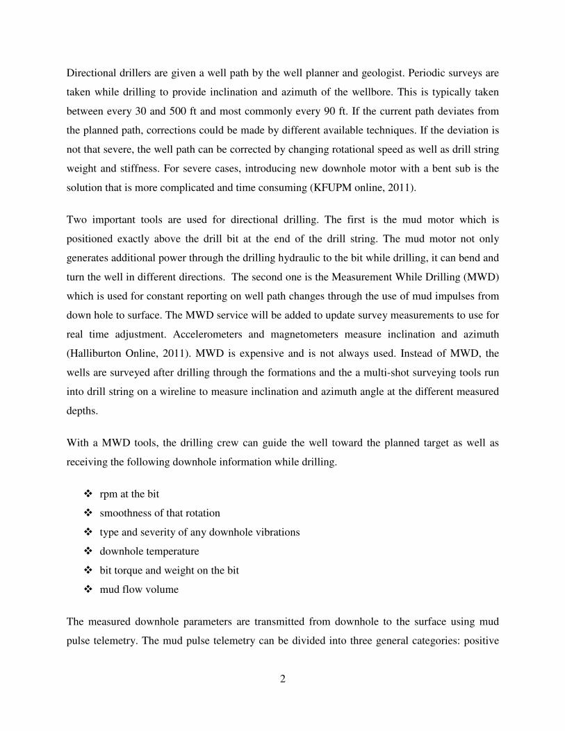
tangent point problem, stabilizer configurations, bent sub model and other considerations for
numerical solutions as shown in Figure 2.1.
Figure 2.1: Schematic of bottom hole assembly (BHA) (Yang, 2008)
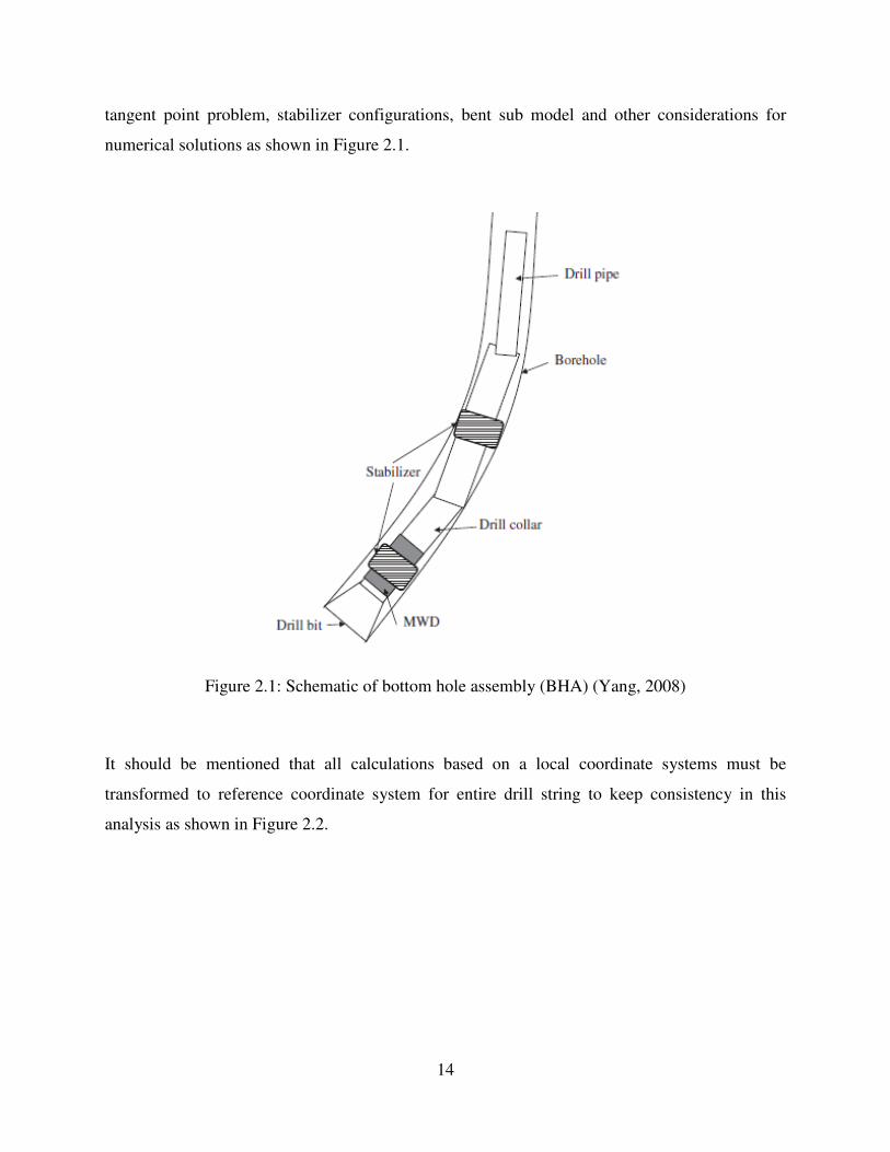
It should be mentioned that all calculations based on a local coordinate systems must be
transformed to reference coordinate system for entire drill string to keep consistency in this
analysis as shown in Figure 2.2.
15
Figure 2.2: Reference and local coordinate systems (Yang, 2008)
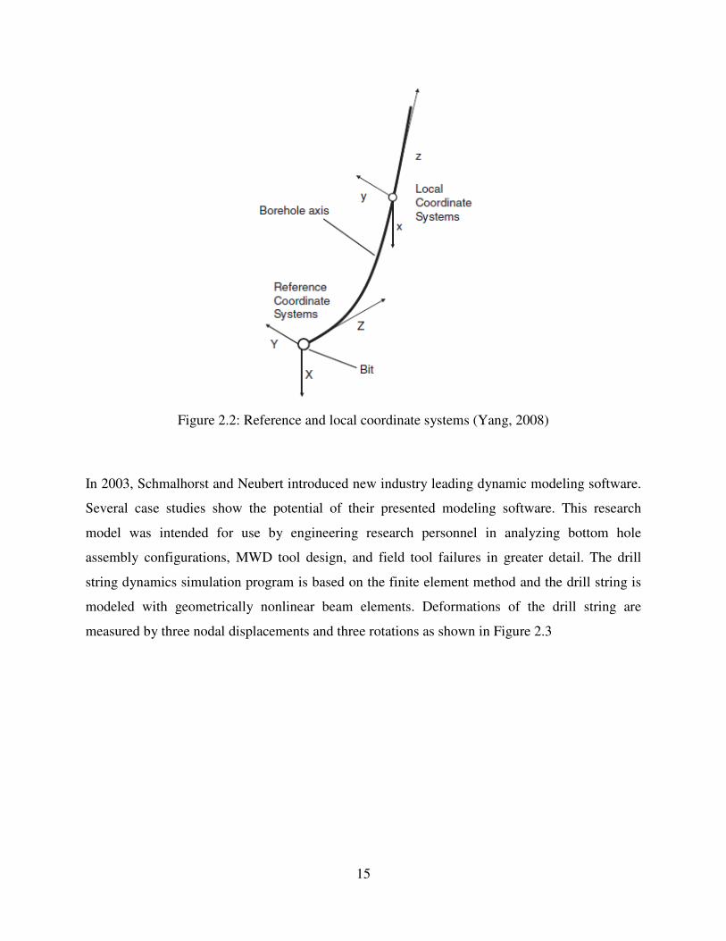
In 2003, Schmalhorst and Neubert introduced new industry leading dynamic modeling software.
Several case studies show the potential of their presented modeling software. This research
model was intended for use by engineering research personnel in analyzing bottom hole
assembly configurations, MWD tool design, and field tool failures in greater detail. The drill
string dynamics simulation program is based on the finite element method and the drill string is
modeled with geometrically nonlinear beam elements. Deformations of the drill string are
measured by three nodal displacements and three rotations as shown in Figure 2.3

16
Figure 2.3: Three dimensional finite beam element (Schmalhorst and Neubert, 2003)
Bueno and Morooka in 1995 modeled the drill string as undeformed elastic beams. They
proposed a methodology to estimate the contact forces generated by the drill string against the
wellbore. The boundary conditions at the bit and the stabilizers are shown on Figure 2.4.
Figure 2.4: Boundary conditions (Bueno and Morooka, 1995)
17
It is assumed that the contact points occur only at the tool joints. The upper boundary condition
(rotary table) is a full restriction of the degrees of freedom. The wellbore was divided into
contact elements with specified spring stiffness.
Newman in 2005 presented a 3-D finite element model which considers the pipe bending inside
the wellbore. The yielding of coiled tubing can be included in this model. The model is able to
calculate the beginning of buckling during drilling operation. He presented the equations and
methodology used in the development of the finite element model and compared the results with
other analytical solutions which are currently in use. Also, he introduced a dynamic finite-
element/ finite-difference model which is a part of a drilling software package. The model
performs a 3-D finite element analysis of drill string at each specific point in time. This analysis
is run repeatedly at short time steps through time using a finite-difference algorithm (Newman
and Procter, 2009).
The behavior of many dynamic systems such as drill string undergoing time-dependent changes
can be described by ordinary differential equations. When the solution for differential
equation(s) of motion of a dynamic system cannot be obtained, a numerical method can be used.
The results are approximated but at least the equation(s) have been solved, (Dukkipati, 2009).

18
CHAPTER THREE: TECHNICAL APPROACH – ANALYTICAL
In this chapter, a new analytical model for torque and drag calculations is presented. The
following new developed model is a soft string model and it ignores any tubular stiffness effects.
This means that the pipe is as a heavy cable lying along the wellbore. This expresses that axial
tension and torque forces along drillstring as well as contact forces that are supported by the
wellbore. The derived equations define the hook load for hoisting, lowering, reaming and back
reaming operations and also the torque for a string in a wellbore. Two sets of equations are
presented, one for the straight well sections such as straight, vertical and horizontal and one for
the curved sections.
3.1 Buoyancy Factor
For torque and drag modeling, it is vital to consider effect of buoyancy force during different
operations. The effective string weight or the string tension in a fluid filled well is the unit pipe
weight multiplied by the buoyancy factor. The buoyancy factor is defined as:
( )iopipe
iioo
AA
AA
−
−−=
ρ
ρρβ 1 (3.1)
where
β: buoyancy factor
ρ: density, kg/m3
A: cross sectional area, m2
Subscripts “o” and “i” refer to the outside and inside of drill string. If there is equal fluid density
inside and outside of the pipe, the buoyancy equation becomes:

19
pipe
o
ρ
ρβ −= 1 (3.2)
Equation 3.2 is most commonly used during drilling operation, whereas Equation 3.1 is used in
cases where there is a density difference between the inside of the string and the annulus like
during cementing, running drill string in the hole as well as under balanced drilling operations.
During well intervention operations, the wellhead may be shut in and an annular pressure applied
and the same buoyancy equation applies, but one must add end reactions caused by the annular
pressure. The buoyancy factor will be discussed further in Chapter 5.
3.2 Straight Sections Modeling
Characteristic of a straight wellbore is that the tension along the string is not contributing to the
normal pipe force, and hence not affecting friction. Straight sections are weight dominated as
only the normal weight component gives friction. Because gravity acts downwards, the wellbore
inclination is used and azimuth changes do not have any contributions. Figure 3.1 shows the
force balance for a straight pipe. The resulting equation uses the following sign convention:
+ means that the pipe is pulled upward
_ means that the pipe is lowered downward
αµαβ sincos12 ±∆+= LwFF (3.3)
where
∆L: length of the element, m

20
Figure 3.1: Force balance for pipe pulling along a straight surface
The first term of Equation 3.3 is referring to the weight of the element and the second term is
referred to as additional frictional force required for moving the pipe element. If inclination α is
equal to zero, it means the pipe section is in a vertical position and the friction term will
diminish. If α becomes 90 degrees, it means the pipe section is located in a horizontal position
and the weight term will diminish.
From Figure 3.2 the axial weight component is:
( ) αα cosLwW ∆= (3.4)
From Figure 3.2, the vertical height is:
αcosLz ∆=∆ (3.5)
Combining Equations 3.4 and 3.5 gives:

21
( ) zwW ∆=α (3.6)
This is an important result. It says that the static axial load of a pipe is equal to the unit weight
multiplied by the projected vertical height. If a vertical well has a depth D, and a deviated well
has the same projected vertical depth, the static drill string weight will be the same for these two
wells.
Figure 3.2: Geometry of the inclined straight pipe
Once the drill string description, the survey data, and the friction coefficient are specified, the
calculation starts at the bottom of the drill string and proceeds stepwise upward. The same
approach is used for the curved section.
If the string is divided to n elements, Fi-1 is the force at bottom of each element and Fi is the
force on top of each element which can be added up the entire wellbore section. Sometimes the
well is filled with different mud weights which results in different buoyancy factor βi in different
sections. If the well is filled with only one drilling fluid with uniform density, all buoyancy
factors βi will be equal. Also, the drill string consists of different components with different unit

22
weights iw such as drill pipe, heavy weight drill pipe and BHA which should all be taken in
consideration in the hook load calculation.
Using the friction coefficient µ, there are two approaches for torque and drag calculations. The
first is assuming one friction coefficient for entire well including both the cased and open hole
sections and try to get the match between field and modeling data. The second is assuming
different friction coefficient for cased and open hole. All µ i can be equal or different depending
on if we have separate open hole or cased hole friction coefficient. If the drill string is divided to
n-1 elements, the general equation for entire drill string in a straight section can be written as:
i
n
i
n LwF )sin(cos2
∑=
±×∆= αµαβ (3.7)
When the friction coefficient is equal to zero, Equation 3.7 shows the static weight of the drill
string in a straight section for different drilling operations.
The same principle applies for the rotating friction, torque. The torque is defined as the friction
coefficient multiplied by normal moment and the tool joint radius. Equation 3.8 shows the torque
loss along the straight section for an element. For this case, the axial force has no contribution to
the torque value. The torque can be considered independent of the direction of rotation.
rLwT ×∆×= αβµ sin (3.8)
For inclination α equal to zero as in a vertical section; no torque loss is present due to the
negligible value of the normal force. For αinclination equal to 90 degree as in a horizontal
section, the maximum torque loss will be happened due to maximum normal force. The Equation
3.9 shows the torque along the drill string in straight section which divided to n-1 elements.

23
i
n
i
n LrwT sin2
∑=
∆×= αβµ (3.9)
It should be mentioned that the drill string in a straight section may consist of different
components which may have different tool joint radius ri. If the bit is interacting with the rock,
the bit torque should be added to all torque loses along drill string in a straight section.
3.3 Curved Sections Modeling
For the curved borehole sections, the normal contact force between string and hole is strongly
dependent on the axial pipe loading. This is therefore a tension dominated process. In the
derivation, it was assumed that the pipe is weightless when computing the friction, but the
weight at the end of the bend is added.
During drilling the wellbore is surveyed at regular intervals. The main outputs are wellbore
inclination and the geographical azimuth. These data are used to calculate depth and horizontal
displacement. A short derivation of the angle change between two survey points follows. P1 and
P2 refer to two measurements spaced along a length ∆L as shown in Figure 3.3
Figure 3.3: Definition of change in direction θ over a length ∆L

24
The angle θ enters the scalar product of the unit vectors e1 and e2 in the direction of the wellbore
tangents at P1 and P2:
θθ coscos. 2121 == eeee (3.10)
From Figure 3.4, the scalar product of the unit vectors may also be expressed as:
θcos.... 21212121 =++= zzyyxx eeeeeeee (3.11)
Figure 3.4: The unit vector e is decomposed along the x-axis, the y-axis, and the z-axis (vertical)

25
From Figure 3.4 the components of e with direction defined by the inclination and azimuth
angles are:
ϕα cos.sin=xe (3.12)
ϕα sin.sin=ye (3.13)
αcos=ze (3.14)
Inserting Equations 3.12, 3.13 and 3.14 into Equation 3.11, the change of angle is related to the
Cartesian coordinates as follows:
( ) 212121 coscoscossinsincos ααϕϕααθ +−= (3.15)
The angle θ is the total directional change. If both inclination and azimuth are changed, the
plane that θ acts in is not constrained to the horizontal or vertical plane. It is therefore a fully
three dimensional representation of the directional change.
Although the inclination α is measured in a vertical projection and the azimuth φ in a horizontal
projection, the dogleg θ is measured in an arbitrary plane, as shown in Figure 3.5. Inspection of
Equation 3.15 reveals that it depends on both inclination and azimuth. These properties will be
used in the following equations when we present the new friction models and are not restricted to
a specific plane.
26
Figure 3.5: The dogleg in 3-dimensional space
The oil industry commonly uses the expression dogleg to describe this directional change. We
may define this in degrees rather than radians:
( ) ( )radDL θπ
180=° (3.16)
The derivative or the slope change is called dogleg severity, and is commonly defined as angle
change per 30 m hole:
( ) 3030/L
DLmDLS
∆=° (3.17)
Knowing the azimuth and inclination at two wellbore positions, the displacements in different
directions will be defined by assuming a curved shape between the two positions. Figure 3.6
shows a vertical projection of the well path.

27
Figure 3.6: Projection of a wellbore in a vertical plane
The relationship between the wellbore, the radius of the circular segment and the angle is:
)( 21 ααα −=∆ RL (3.18)
It should be noted the above inclination angles are in radians. The vertical projected height is:
11
2121
)sin(sinsinsin
αα
αααα αα
−
−∆=−=∆
LRRV (3.19)
The vertical projected height will be used to compute the axial pipe weight. To find the changes
in the north and east coordinate, the wellbore trajectory is projected onto a horizontal plane, as
shown in Figure 3.7:

28
Figure 3.7: Projection of wellbore in a horizontal plane. In this projection the wellbore is
assumed to be circular.
From the horizontal projection in Figure 3.7, the circular segment can be expressed as:
12 coscos αα ϕϕ RRD −=∆ (3.20)
This is the distance of the circular projection of the wellbore in the horizontal plane, and is
connected to the radius ϕR and azimuth angles by the relation:
)( 21 ϕϕφ −=∆ RD (3.21)

29
The changes N∆ and E∆ now follow from Figure 3.7:
)sin(sin 21 ϕϕϕ −=∆ RN (3.22)
and
)cos(cos 12 ϕϕϕ −=∆ RE (3.23)
The complete expressions obtain from inserting for φR and ∆D are;
( )( )( )( )2121
2112 sinsincoscos
ϕϕαα
ϕϕαα
−−
−−∆=∆ LN (3.24)
and
( )( )( )( )2121
1212 coscoscoscos
ϕϕαα
ϕϕαα
−−
−−∆=∆ LE (3.25)
Equations 3.24 and 3.25 will not be used in this derivation. They are given for the sake of
completeness, and are used to compute the geographical position of any point of the wellbore.
With reference to Figure 3.4, we may assume that the x-axis points north and the y-axis points
east. Defining the unit vector to have a length ∆L, the displacements for a straight section can be
defined as:
Vertical projection (to compute axial pipe weight):

30
αcosLV ∆=∆ (3.26)
Horizontal projections in the northern and eastern directions are:
ϕα cossinLN ∆=∆ (3.27)
and
ϕα sinsinLE ∆=∆
(3.28)
Again, the horizontal projections are not used in the derivation, but presented to define the
complete set of equations to define the geographical positions of the borehole.
For the curved borehole sections, the normal contact force between the drill string and wellbore
is strongly dependent on the axial pipe loading. This is therefore a tension dominated process.
In e.g. a short bend, the tension is often much larger that the weight of the pipe inside the bend.
In the following derivation we will assume that the pipe element is weightless when we compute
the friction, but we add the weight at the end of the bend. Figure 3.8 shows an element that is
pulled along a curved surface. Performing a force balance in the Z- and X- directions results in:
Z-direction:
θdFdN ×= (3.29)
X-direction:

31
θµ FddF ×= (3.30)
Figure 3.8: Element pulled along curved surface
Integrating the force equation between the upper and lower position gives:
(Defining θ = θ2 - θ1):
θµ±= eFF 12 (3.31)
The following sign convention applies:
+ means that pipe is pulled upwards
- means that the pipe is lowered
For a rotating string, the same contact force applies, only friction direction is tangential. The
torque for the pipe that is not pulled or lowered is simply:
θµµ 1rFrNT == (3.32)
32
Furthermore, the dogleg angle θ depends both on the wellbore inclination and the azimuth.
Because the pipe will contact either the high side or the low side of the wellbore, its contact
surface is given by the dogleg plane.
For build-up, drop-off, side bends or combination of these, the axial force becomes:
−
−∆+=
±
12
1212
sinsin
αα
ααβ
θµLweFF (3.33)
where + means hoisting and – means lowering of the pipe.
The torque for the bend is defined in Equation 3.34 as:
θµµ 1rFrNT == (3.34)
Friction for any wellbore shape can thus be computed by dividing the well into straight and
curved elements. The forces and torques are summed up starting from bottom to top of the well.
For the entire curved section the axial force can be calculated as follow:
∑= −
−±
−
−
−×∆+×=
n
i ii
ii
iiiin LweFF ii
2 1
11
sinsin
αα
ααβ
θµ (3.35)
Equation 3.36 shows torque losses for the entire curve section
33
i
n
i
iiin FrT θµ∑=
−×=2
1 (3.36)
3.5 Combined Axial Motion and Rotation
The solutions presented in sections 3.3 and 3.4 must be modified if a combined motion takes
place. Aadnoy and Andersen (2001) showed how the frictional capacity is decomposed into the
two directions, axial motion and rotation. The effect of combined motion is well known, for
example when rotating a liner for running easier into the hole. A high rotational speed reduces
axial drag considerably. During tripping operations an overpull may occur due to tight hole
conditions. The remedy action is typically to rotate the drill string while pulling or lowering. In
the oilfield, the considerable difference can be observed between measured hook loads while
tripping in/out and the reaming/back reaming operation.
Aadnoy and Andersen (2001) showed how the frictional capacity is disintegrated into the two
directions, axial and rotational movements. Figure 3.9 shows a pipe section with weight of Lw∆ .
If it is pulled along a surface, the drag will be equal to the normal force, Lw∆ multiplied with the
coefficient of friction Lw∆µ . If the pipe is rotated instead, the torque ratio, T/r is also equal
to Lw∆µ . Thus, the weight and friction coefficient results in the same frictional resistance
regardless of whether the movement is axial or rotational.
Figure 3.9: Drag and torque for a pipe element

34
In the following a simple model for combined motion is developed which shows the effect of
rotation and axial movement on well friction as a function of tripping velocity and rotary speed.
It can be multiplied by friction coefficient in sine and cosine form which results in a reduction in
the value of the friction force.
During combined motion, the axial velocity is Vh, and the tangential pipe speed is Vr. As derived
in following, these give a resultant velocity V. The angle between the two velocities is defined in
Figure 3.10 below.
Figure 3.10: Relationship between hoisting/lowering and rotational speed
Figure 3.10 shows the velocities on the pipe surface for combined motion. They are given by the
following Equations:
)(60
)(2
:
)/(tan
)/(/
rpmNmr
V
or
smrotationtoduespeedgentialV
smspeedloweringhoistingV
rr
r
h
×=
=
=
π
(3.37)

35
We assume that the amount of friction axially/tangentially is proportional to the relative
velocities. The angle of the friction vector is:
= −
r
h
V
V1tanψ (3.38)
For a straight pipe section, the axial and the tangential friction forces are:
αβµ
αβµ
sin
sin
Lwr
T
LwFFaxial
∆×=
∆×=
(3.39)
For pure hoisting/lowering or pure rotation, the frictional forces are the same for axial drag and
rotation. For combined motion, the resultant frictional force is constant. Figure 3.11 shows this.
Figure 3.11: Relationships between torque and drag for straight pipe sections
First determine the hoisting/lowering speed, the rotational speed, and compute the angleψ .
Then compute the resulting torque and drag as follows:
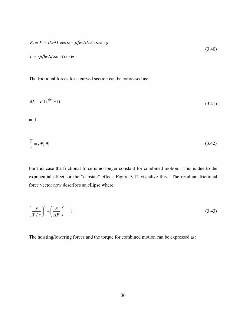
36
ψαµβ
ψαµβαβ
cossin
sinsincos12
LwrT
LwLwFF
∆=
∆±∆+=
(3.40)
The frictional forces for a curved section can be expressed as:
)1(1 −=∆± θ
eFF (3.41)
and
θµ 1Fr
T= (3.42)
For this case the frictional force is no longer constant for combined motion. This is due to the
exponential effect, or the “capstan” effect. Figure 3.12 visualize this. The resultant frictional
force vector now describes an ellipse where:
1/
22
=
∆+
F
x
rT
y (3.43)
The hoisting/lowering forces and the torque for combined motion can be expressed as:

37
Figure 3.12: Relationship between torque and drag for bend
−
−∆+−+=
±
12
12
112
sinsinsin)1(
αα
ααβψ
θµwLeFFF (3.44)
ψθµµ cos1rFrNT == (3.45)
When is equal to 90 degree, it means there is no rotation during axial movement, and when
equal to 0 degree means there is no axial movement during rotation.
The torque and drag equations can be written for combined motion as follow:
For entire straight section:
i
n
i
n
i
in LwLwF sinsincos2 2
ψµαβαβ ××∆±∆=∑ ∑= =
(3.46)
and

38
i
n
i
n LrwT cossin2
∑=
×∆×= ψαβµ (3.47)
For entire curved section:
( )∑= −
−±
−
−
−×∆+×−×=
n
i ii
ii
iiiiin LweFF i
2 1
11
sinsinsin1
αα
ααβψ
θµ (3.48)
and
iiiii
n
i
n FrT ψθµ cos1
2
××= −=
∑ (3.49)
3.5 Application of the New Model
The models presented can be applied both during drilling by computing the friction for each
survey point, or by dividing the entire well into a number of elements. Three cases will be
presented where entire wells are analyzed.
3.5.1 Case A: Analysis of a Two Dimensional S-shaped Well
This example will demonstrate the application of the model, and also identify some frictional
effects.
Figure 3.13 shows an S-shaped well that is drilled in a vertical plane. The total length is 2111
m, and the drill string consist of 161 m of 8” 3” drillcollars (2.13 kN/m) and 1950 m of 5”-19.5
lbs/ft drillpipe (0.285 kN/m). The drillcollar radius is 0.1 m, and the drill string connection
radius is 0.09 m. The well is filled with 1.3 SG drilling mud and the coefficient of friction is

39
estimated to be 0.2. The bottom-hole-assembly starts out just below the drop-off section, and is
vertical. For this case there is no change in azimuth, and the dogleg of Equation 3.15 becomes
equal to the change in inclination.
The buoyancy factor is calculated as follow:
Pipe density is 7.8 SG.
833.08.7
3.11 =−=β
Assuming that the drill bit is off bottom, we will compute the forces starting from bottom of the
well. For simplicity, the frictional factors of the bends are:
=== ±
±
±
855.0
17.1157.0180
452.0
eee
π
µθ
The net weight of the bottom-hole-assembly:
kNmm
kN28616113.2833.0 =××
The buoyed pipe weight:
m
kN
m
kN237.013.2833.0 =×

40
Figure 3.13: Geometry of S-shaped well
The axial forces along drill string were calculated for different points such as well bottom,
bottom of drop-off section, bottom of sail section, top of sail section, top of build-up section and
top well as shown in Table 3.1

41
Table 3.1: Forces in the drill string during hoisting and lowering
Position Static weight(kN) Hoisting (kN) Lowering(kN)
well bottom 0 0 0
bottom drop-off
section
286 286 286
bottom sail section 286+0.237×120=
315.5
286×1.17+28.5=
363
286×0.855+28.5=
272.9
top sail section 315.5+0.237×925=
533.6
363+0.237×1308( cos
55˚+0.20sin55˚)= 626
272.9+0.237×1308( cos 55˚-
0.20sin55˚)= 558.3
top buildup
section
533.6+0.237×120=
562
626×1.17+28.5=
760.9
558.3×0.855+28.5=
511.7
top well 562+0.237×335=
651.5
760.9+79.5=
850.3
511.7+79.5=
591.1
When calculating torque, we will use two scenarios:
1) with bit off bottom
and
2) with a weight on the bit of 90 kN
Table 3.2 shows all calculations related to all the torque for on bottom and off bottom interest
points. The static weight for the second case is simply obtained by subtracting the bit force
throughout the string.
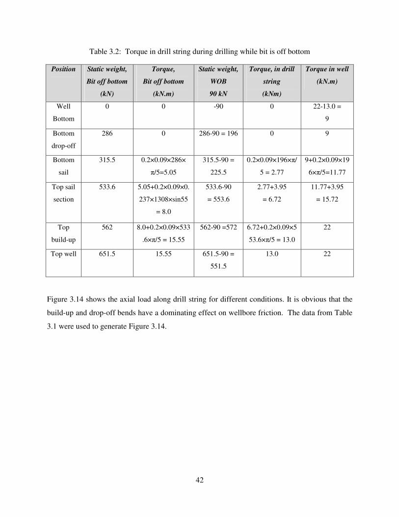
42
Table 3.2: Torque in drill string during drilling while bit is off bottom
Position Static weight,
Bit off bottom
(kN)
Torque,
Bit off bottom
(kN.m)
Static weight,
WOB
90 kN
Torque, in drill
string
(kNm)
Torque in well
(kN.m)
Well
Bottom
0 0 -90 0 22-13.0 =
9
Bottom
drop-off
286 0 286-90 = 196 0 9
Bottom
sail
315.5 0.2×0.09×286×
π/5=5.05
315.5-90 =
225.5
0.2×0.09×196×π/
5 = 2.77
9+0.2×0.09×19
6×π/5=11.77
Top sail
section
533.6 5.05+0.2×0.09×0.
237×1308×sin55
= 8.0
533.6-90
= 553.6
2.77+3.95
= 6.72
11.77+3.95
= 15.72
Top
build-up
562 8.0+0.2×0.09×533
.6×π/5 = 15.55
562-90 =572 6.72+0.2×0.09×5
53.6×π/5 = 13.0
22
Top well 651.5 15.55 651.5-90 =
551.5
13.0 22
Figure 3.14 shows the axial load along drill string for different conditions. It is obvious that the
build-up and drop-off bends have a dominating effect on wellbore friction. The data from Table
3.1 were used to generate Figure 3.14.

43
Figure 3.14: Torque and drag for the S-shaped well
This is further seen in Figure 3.15, which shows the torque calculations along drill string. When
the bit force is applied, weight on the bit, the tension in the string decreases, leading to less string
torque in the curved sections.

44
Figure 3.15: Torque along drill string during off/on bottom conditions
Figure 3.15 shows the reduction in string tension that leads to a reduced string torque. The
numerical values are given in Table 3.2. When the bit force, weight on the bit, is applied, the
driller observes an increase in torque of 6.56 kNm to a total value of 22 kNm. However, due to
the reduction in string torque, the bit torque is actually 9 kNm. From this example it is obvious
that the bit torque is always higher than the torque increase at surface for a deviated well.

45
3.5.2 Case B: Analysis of a 3-dimensional Well
Figure 3.16 shows this well. It is complex as its direction changes in the 3-dimensional space.
The analysis is similar to the analysis of Case A, except that the bends are not restricted to a
vertical plane, but in a 3-dimensional plane.
X
Y
Z
500
1052
1512
1752
20632104
40
0
25
73
Figure 3.16: 3-dimensional well shape
The pipe data are taken the same as for Case A. Performing the analysis, the results are shown in
Figure 3.17. Clearly, a different friction picture is seen in these wells which consist of 3 bends.
By increasing the total angle change of a well, the friction increase significantly.

46
500 1000
1000
2000
3000
)(mMD
)(kNForce
)(kNmTorque
0 10 20
0
500
1100
1700
2075
2865
HoistingLoweringStatic
768576463
Build-up
Straight Inclined
Build-up
with
Right Side Bend
Build-up
with Left Side Bend
Straight Inclined
BHA
Vertical
5.13
ueStaticTorq
Figure 3.17: Wellbore friction for 3-dimensional well
3.5.3 Case C: Combined Motion in 3-dimensional Well
Some well operations are performed with combined motion. For high inclination wells it is
common to rotate the liner in order to bring it to the desired depth. In the following we will
investigate the frictional picture during such events.

47
Again assuming the same pipe data we will investigate the effect of combined motion in the well
of Case B. The pipe is rotated at 100 rpm, and it is hoisted or lowered at 0.27 m/sec. From
Equation 3.38, the angle between the axial and tangential pipe velocities becomes 30 degrees.
Using Equations 3.39 and 3.40, the friction for combined motion is computed. The results are
shown in Figure 3.18, which compares pure hoisting/lowering with combined motion. A clear
reduction in drag is observed.
Figure 3.18: Comparison between pure hoisting/lowering and combined motion
Both when hoisting and lowering the string a reduced axial friction is seen. It is seen that the
limiting value, ψ → 0˚, which is obtained with low hoisting speed or high rotational speed, both

48
the hoisting and the lowering forces approached the static pipe weight. In other words, high
rotation removes the axial friction.
Figure 3.19: Torque along drill string with combined motion
Using equations 3.39 and 3.50, the torque during hoisting and lowering is compared to the static
(bit off bottom) torque. During hoisting while back reaming the torque decreases slightly,
whereas during lowering the torque decreases more as shown in Figure 3.19.
The examples above serve to show the potential of torque and drag analysis using the simple 3-
dimensional models presented herein. To determine the coefficients of friction from field data,
not only can the hoisting-lowering-rotation models be used, but also the models for combined
motion. This should improve the determination of the frictional forces in a well, and also in
application to any well operation.

49
CHAPTER FOUR: TECHNICAL APPROACH- FINITE ELEMENT
The finite element method is one of the most applied numerical methods for solving differential
equations with complicated geometries (Reddy 2005). In this method problems are divided into a
set of logical steps that can be implemented on a computer and solved for a wide range of input
data. For example in drilling engineering, the finite element divides the entire drill string to
finite number of small elements. Every smaller drill string element has simpler form to analyze
and is not as complex as the entire drill string. The simulation of all the smaller elements leads to
good approximation for the entire drill string analysis. At every node a polynomial expression
for the equations of motion is generated which allows an accurate result at that specific point.
For finite element analysis, equilibrium exist between the external applied forces and the internal
forces. A compatibility of displacements and relationships between loads applied and
deformations is reached (Reddy, 2005). In finite element analysis, boundary limitations are set
for a given problem. If no boundary conditions are set for the system, it is treated as a rigid body
floating in space. The boundary conditions have a strong effect on the solutions values. Different
analysis of the same problem can be done with different boundary conditions simply by changing
them. This could be done by changing the node conditions and placements or the material
properties (Dukkipati, 2009).
In this research, an attempt was made to calculate the torque and drag from a generalized
displacement of the drill string model which was used to predict the lateral and axial vibrations.
The drill string has been thought of as a very long, unbalanced rotor of variable geometry
constrained within a continuous journal bearing of variable clearance and rigidity. The dynamics
of such a system is a rotor dynamic problem, so an approach that has been used effectively to
solve rotor dynamics problems in other industries is also adapted for the present research. This
requires developing the equations of motion beginning with Hamilton’s principle, and then
solving them using the finite element method for torque and drag calculations (Dykstra, 1996).

50
4.1 Hamilton’s Principle
Hamilton’s principle states that the motion of a particle is such that the kinetic and potential
energies of the particle and the work done by the forces which act on it are related as shown the
Equation 4.1:
( ) ∫∫∆∆
=+−tt
Wpk 0δδ (4.1)
In this expression, k is the kinetic energy which has components due to velocities of translation
and rotation. p is the potential energy or strain energy and is defined in terms of stressσ and
strain ε. W is the work done by forces including gravity, unbalanced mass and viscous force.δ is
the variation operator in Equation 4.1 (Dykstra, 1996).
4.2 Shape Function
In finite element a beam element is defined by the two nodes being used, with six degrees of
freedom (DOF) at each node; three displacements ),,,( tzyxu and three rotations. This yields a
total of 12 DOF for each element. A three dimensional beam model is used with six degrees of
freedom for each node as shown in Fig 4.1: two transverse displacement (U2 or U8, U3 or U9),
two bending rotations (U5 or U11, U6 or U12), one torsional rotation and one axial displacement
(U1 or U7, U4 or U10) as shown by Wu et al., (2011).

51
Figure 4.1: Generalized displacement for a beam element
4.3 The Dynamic Equations
The dynamic equations will be obtained by substituting the interpolation functions into the
energy and work (Hamilton) expressions and evaluating the integrals. This results in the
following discrete system of equations for an element which can be expressed as Equation 4.2
representing the matrix form of the equation of motion for a multi-degree of freedom system
(Wu et al., 2011).
[ ] [ ] [ ] FUKUCUM =++ &&& (4.2)
[ ]M , [ ]C and [ ]K represents the mass, damping and stiffness matrixes respectively. If these
matrixes are time independent and remain unchanged during integration, the dynamic system
will be linear. For nonlinear dynamic systems, if they vary with the time, they must be modified
during the integration. Also, the vectors U , U& , U&& and F represents generalized
displacements, velocities, accelerations and forces acting on two nodes of an element,
respectively. They can be shown in form of transpose as follow:
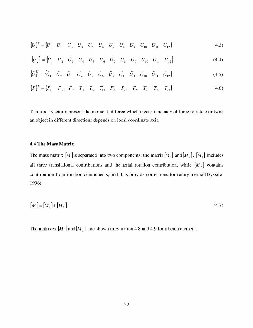
52
121110987654321 UUUUUUUUUUUUUT
= (4.3)
121110987654321 UUUUUUUUUUUUUT
&&&&&&&&&&&&& = (4.4)
121110987654321 UUUUUUUUUUUUUT
&&&&&&&&&&&&&&&&&&&&&&&&&& = (4.5)
232221232221131211131211 TTTFFFTTTFFFFT
= (4.6)
T in force vector represent the moment of force which means tendency of force to rotate or twist
an object in different directions depends on local coordinate axis.
4.4 The Mass Matrix
The mass matrix [ ]M is separated into two components: the matrix [ ]1M and [ ]2M . [ ]1M Includes
all three translational contributions and the axial rotation contribution, while [ ]2M contains
contribution from rotation components, and thus provide corrections for rotary inertia (Dykstra,
1996).
[ ] [ ] [ ]21 MMM += (4.7)
The matrixes [ ]1M and [ ]2M are shown in Equation 4.8 and 4.9 for a beam element.
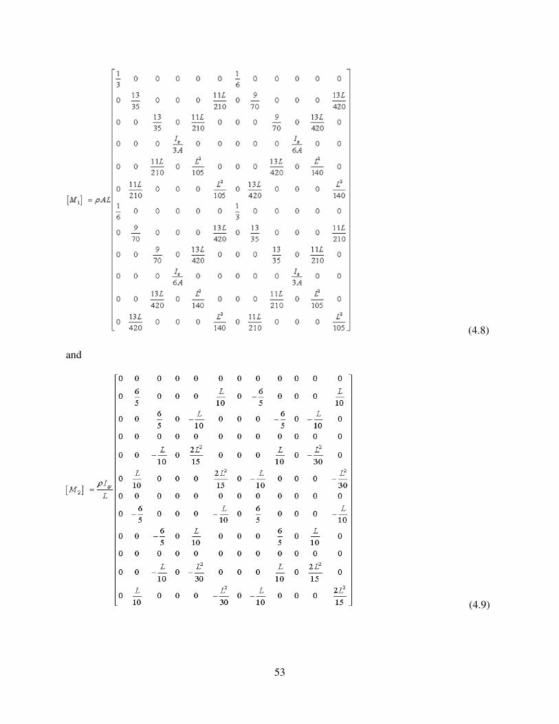
53
(4.8)
and
(4.9)

54
4.5 The Stiffness Matrix
The stiffness matrix is separated into linear and nonlinear contributions: [ ]LK and [ ]NK .
[ ] [ ] [ ]NL KKK += (4.10)
The linear contributions to stiffness results from strain energy expression (Wu et al., 2011). The
linear stiffness matrix has been shown in Equation 4.11.
(4.11)
The components in the nonlinear stiffness matrix arise due to some terms in the strain-
displacement relation presented in Equation 4.12.
[ ] [ ] [ ] [ ]NTNANAN KKKK ++=21
(4.12)
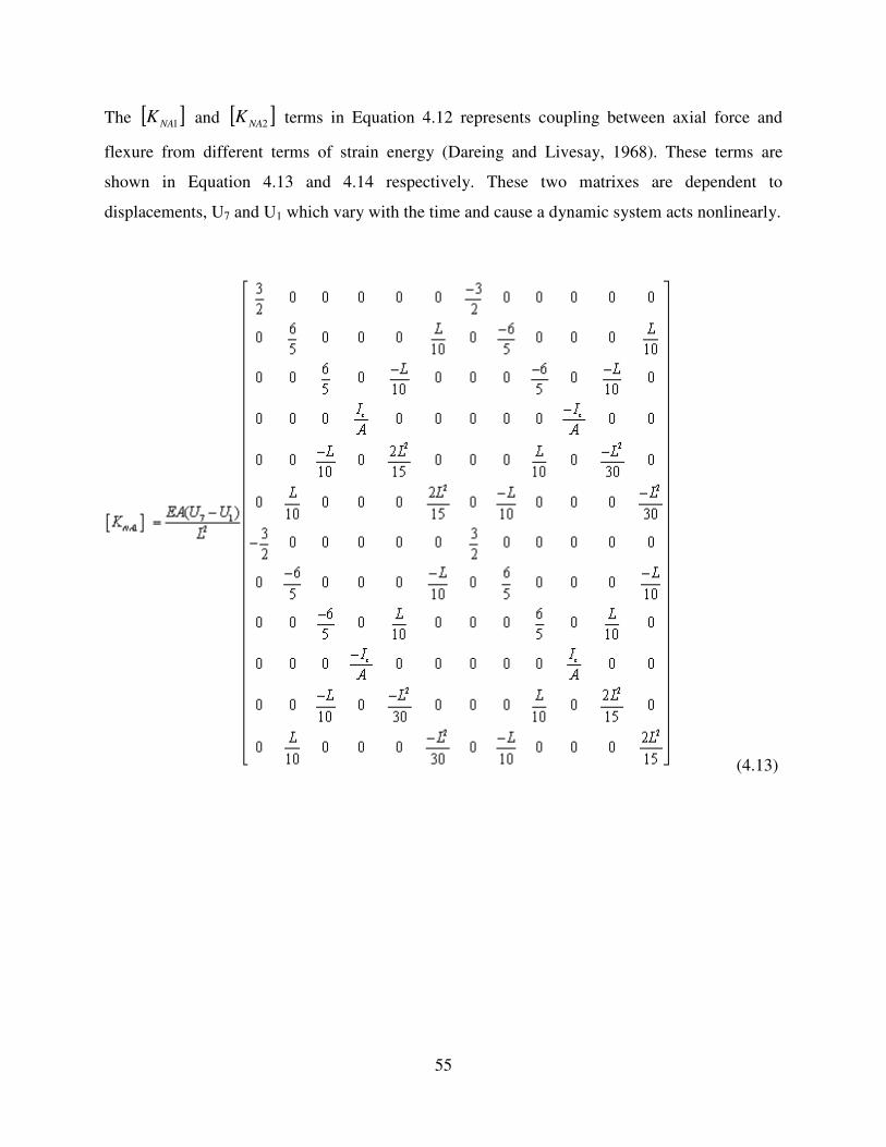
55
The [ ]1NAK and [ ]2NAK terms in Equation 4.12 represents coupling between axial force and
flexure from different terms of strain energy (Dareing and Livesay, 1968). These terms are
shown in Equation 4.13 and 4.14 respectively. These two matrixes are dependent to
displacements, U7 and U1 which vary with the time and cause a dynamic system acts nonlinearly.
(4.13)

56
(4.14)
The [ ]NTK represents coupling between torsion and flexure which is also a geometric stiffness
contribution, but unlike the axial force-flexure matrices the component addresses do not coincide
with those in linear stiffness matrix (Dareing and Livesay, 1968). The vectors U10 and U4
represent rotation terms related to element rotations along the X-axis as shown in Figure 4.1.
(4.15)

57
4.6 The Damping Matrix
The damping matrix includes two parts: [ ]DC and [ ]NC .
[ ] [ ] [ ]ND CCC += (4.16)
The matrix [ ]DC is a dissipative damping matrix. It means they remove energy from the system.
The [ ]DC considered in this research is that of Rayleigh (Besaisow, et. al, 1985). It is assumed to
be appropriate because the drill string is immersed in a fluid which is generally viscous. Rayleigh
damping is obtained from linear combination of the mass and stiffness matrices.
[ ] [ ] [ ]LD KMC βα += (4.17)
Where α and β are weighting parameters that allow system damping to be adjusted.
(4.18)

58
The matrix [ ]NC is a non-dissipative damping matrix, or a gyroscopic matrix as shown in
Equation 4.18 (Dykstra, 1996).
In all above matrixes, GE ν、 、 is drill string elastic modulus, Poisson’s ratio and shear
modulus respectively; ,x y
I I and zI are on the x ,y and z-axis area moment of inertia of drill string
element; Ω the drill string rotation speed; zJ is the polar moment of inertia of drill string
element on z-axis . Also, ρ, A and L are density, cross sectional area and length of drill string
element.
4.7 Force Vector
Dykstra in 1996 presented the external forces which include gravity, imbalanced mass and
frictional interaction with the wellbore. The gravity force is the equivalent generalized force for
the loading due to distributed mass. This is equivalent to setting the virtual work done on the
continuous structure by the distributed loads (concentrated forces and moments) to the work
done on the discrete model by the generalized nodal forces.
The contributions to the external force vectors due to imbalanced forces are obtained just as the
gravity forces were. The equivalent nodal forces for the distributed imbalance loads include both
forces and moments. Imbalanced force occurs when the center of gravity does not coincide with
the rotary center of the drill string. In this research, the imbalanced force is neglected.
Dykstra in 1996, showed the gravity force vector as Equation 4.19. This gravity forces vector are
equivalent to both concentrated forces and moments for a specific element as shown in Figure
4.2.
[ ]
−−−−−=
12000
2212000
22
22LwLwLwLwLwLw
Fyyxyyx
gravity (4.19)
Where

59
α
α
sin
cos
×=
×=
ww
ww
y
x
(4.20)
Figure 4.2: Distributed forces due to gravity on an inclined element
For friction force consideration in force vector it is necessary to estimate the normal force at each
element. Figure 4.3 shows the normal force FN acting on drill string element which is very
important in torque and drag calculations.
Figure 4.3: The forces applied on an element of drill string
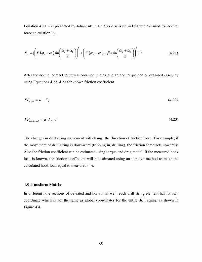
60
Equation 4.21 was presented by Johancsik in 1985 as discussed in Chapter 2 is used for normal
force calculation FN.
( ) ( ) 2/1
2
12121
2
12121 ]
2sin
2sin[
++−+
+−=
ααβαα
ααϕϕ wFFFN (4.21)
After the normal contact force was obtained, the axial drag and torque can be obtained easily by
using Equations 4.22, 4.23 for known friction coefficient.
Naxial FFF ⋅= µ (4.22)
rFFF Nrotational ⋅⋅= µ (4.23)
The changes in drill string movement will change the direction of friction force. For example, if
the movement of drill string is downward (tripping in, drilling), the friction force acts upwardly.
Also the friction coefficient can be estimated using torque and drag model. If the measured hook
load is known, the friction coefficient will be estimated using an iterative method to make the
calculated hook load equal to measured one.
4.8 Transform Matrix
In different hole sections of deviated and horizontal well, each drill string element has its own
coordinate which is not the same as global coordinates for the entire drill string, as shown in
Figure 4.4.

61
Figure 4.4: Difference between element local coordinate system and global coordinate system
To include inclination and azimuth angles in torque and drag calculations, it is required to define
a matrix to transform the element coordinate system xyz to the global coordinate system XYZ.
The transform matrix defined as shown in Equation 4.24 includes inclination and azimuth angles
for each element. It is necessary for all matrixes such as mass, stiffness and damping as well as
and vectors such as displacement, velocity, acceleration and forces to be transformed from their
local coordinate to the global coordinate.
In Equation 4.25, α and φ represent inclination and azimuth, Uz, Ux, Uy, Ez, Ex and Ey are three
translations and three rotations in the global system and uz, ux, uy, εz, εx and εy are three
translations and three rotations in the local system (Wu et. al., 2011).
−
−
−
−
=
y
x
z
y
x
z
y
x
z
y
x
z
u
u
u
E
E
E
U
U
U
ε
ε
ε
φφαφα
φφαφα
ααφφαφα
φφαφα
αα
cossincossinsin
sincoscoscossin
0sincos
0
0
cossincossinsin
sincoscoscossin
0sincos
(4.24)

62
Also in dealing with the initial conditions and boundary conditions of work, we often need the
coordinates of each element in local coordinate system. At this point it is required load,
displacement, velocity column matrix to be transformed from global coordinate system to the
local coordinate system. Coordinate transformation appears multiple times in a dynamic model
to approach a solution.
4.9 Global Matrix
In order to get the solution of the system, the global matrix should be formed using such element
mass matrix like Equation 4.25.
[ ]11 126 6 6 6
21 226 6 6 6
i i
i
i i
M MM
M M
× ×
× ×
=
(4.25)
The assembly process for entire drill string can be shown in the following Equation 4.26 taking
mass matrix as an example.
[ ]
1 1
11 12
1 1 2 2
21 22 11 12
2 2
21 22
1
22 11 12
1
21 22 11
1 1
11 12
1 1
21 22 11 12
2
i i i
i i i
N N
N N N N
M M
M M M M
M M
M M M
M M MM
M M
M M M M
M
−
+
− −
− −
+
+
+
+ =
+
+
L L
L L L L
L L
L L
L L L
L
L L
L L
1 22
N NM
(4.26)
For the force vector, the global vector for a single element can be written as follow:
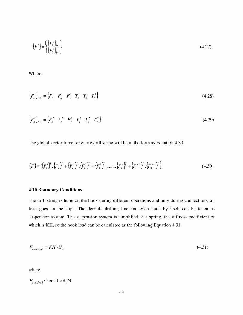
63
=×
×
162
161
i
i
i
F
FF (4.27)
Where
111111
161 yxzyxz
iTTTFFFF =
× (4.28)
222222
162 yxzyxz
iTTTFFFF =
× (4.29)
The global vector force for entire drill string will be in the form as Equation 4.30
TnTnTnTTTTTFFFFFFFFF 1
2
1
12
3
1
2
2
2
2
1
2
1
1 ,,.......,,, +++++= (4.30)
4.10 Boundary Conditions
The drill string is hung on the hook during different operations and only during connections, all
load goes on the slips. The derrick, drilling line and even hook by itself can be taken as
suspension system. The suspension system is simplified as a spring, the stiffness coefficient of
which is KH, so the hook load can be calculated as the following Equation 4.31.
1
zhookload UKHF ⋅= (4.31)
where
hookloadF : hook load, N

64
1
zU : the axial translation of the first node, m
The main boundaries are at the rotary table, drill bit and stabilizers as shown in the Figure 4.5.
Figure 4.5: Main boundaries on the drill string in the wellbore
At the rotary table, the radial displacement is constrained but axial displacement and rotation
around drill string axis are released. For the rotary table (or top drive) at surface the following
boundary conditions for the different modes is considered:
(1) rotating drilling (including common rotary drilling and top drive system)
01 =xU
01 =yU
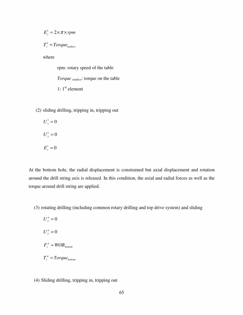
65
rpmE z ××= π21
surfacez TorqueT =1
where
rpm: rotary speed of the table
Torque surface: torque on the table
1: 1st element
(2) sliding drilling, tripping in, tripping out
01 =xU
01 =yU
01 =zE
At the bottom hole, the radial displacement is constrained but axial displacement and rotation
around the drill string axis is released. In this condition, the axial and radial forces as well as the
torque around drill string are applied.
(3) rotating drilling (including common rotary drilling and top drive system) and sliding
0=n
xU
0=n
yU
bottom
n
z WOBF =
bottom
n
z TorqueT =
(4) Sliding drilling, tripping in, tripping out

66
0=n
xU
0=n
yU
0=n
zF
0=n
zT
where
n: last element
At the stabilizers: radial displacement is constrained and axial displacement and rotation around
drill string axis is released;
(5) For any operation mode
0=i
xU
0=i
yU
The drill string is constrained in the wellbore all the time as shown in Figure 4.6. In the local
coordinate system o-xyz, lateral displacements ux and uy of centerline should satisfy the
following Equation.
duu yx ∆≤+ 22 (4.32)
Where
( )2
dDD
−=∆ : Clearance between the BHA components and the wellbore wall
D: diameter of the wellbore

67
d: outer diameter of BHA.
If the above equation is not satisfied, the BHA will contact the wellbore wall.
Figure 4.6: Constraint relations between drill string and wellbore
4.11 Solution Method
In this study, as solution method, the implicit method is used to get the displacement values
directly as solutions from the equation of motion directly. For implicit schemes, the following
solution methods are available.
Houbolt
Newmark Beta
Park Stiffly stable
Wilson-Theta
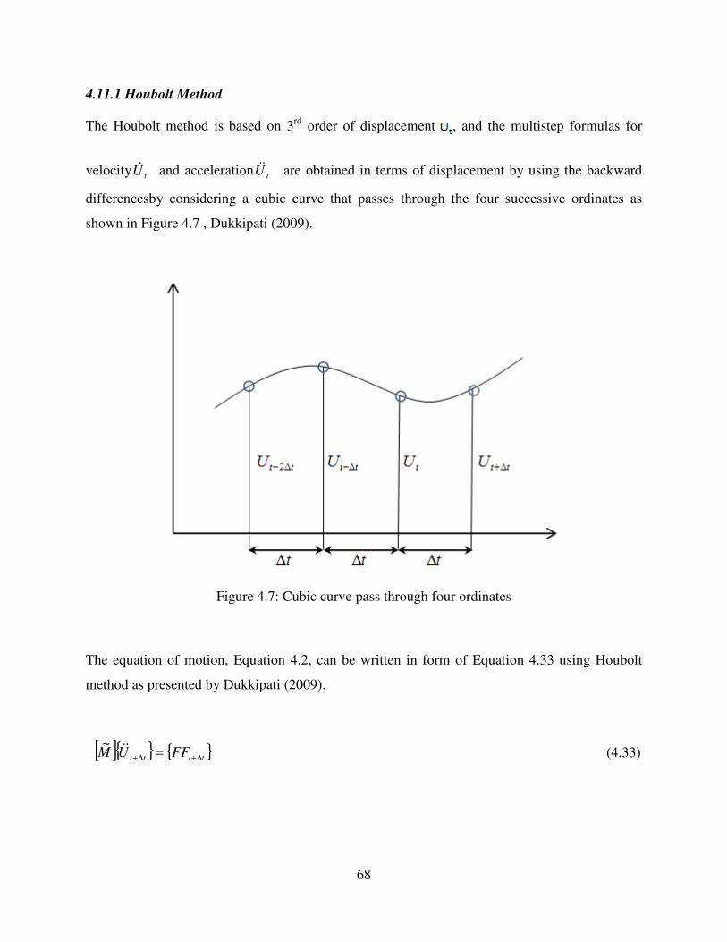
68
4.11.1 Houbolt Method
The Houbolt method is based on 3rd order of displacement , and the multistep formulas for
velocity tU& and acceleration tU&& are obtained in terms of displacement by using the backward
differencesby considering a cubic curve that passes through the four successive ordinates as
shown in Figure 4.7 , Dukkipati (2009).
Figure 4.7: Cubic curve pass through four ordinates
The equation of motion, Equation 4.2, can be written in form of Equation 4.33 using Houbolt
method as presented by Dukkipati (2009).
[ ] tttt FFUM ∆+∆+ =&&~
(4.33)

69
Where [ ]M~
, the effective mass matrix and ttFF ∆+ is the effective force vector as shown in
following equations:
[ ] [ ] [ ] [ ]KCt
Mt
M +∆
+∆
=6
112~2
(4.34)
and
[ ] [ ] [ ] [ ]
[ ] [ ] tt
ttttttt
UCt
Mt
UCt
Mt
UCt
Mt
FFF
∆−
∆−∆+∆+
∆+
∆
+
∆+
∆−
∆+
∆+=
22
22
3
11
2
3435
(4.35)
The Houbolt method has some disadvantages which does not allow this method used for drill
string dynamic system. In Equation 4.35, there is no direct method to find ttU ∆− and ttU ∆−2
initially which makes this method non-self starting. Also, it requires large computer storage to
store displacement for the previous time steps (Dukkipati, 2009).
4.11.2 Newmark Beta Method
This method is based on this assumption that acceleration varies linearly between two instants of
time. Two parameters of α and β are used in this method which can be changed to meet the
requirements of a particular problem (Dukkipati, 2009). The effective mass matrix [ ]M~
and
effective force vector ttFF ∆+ are given by the following:
[ ] [ ] [ ] [ ]KCt
Mt
M +∆
+∆
=β
α
β 2
2~ (4.36)
70
and
[ ] [ ] [ ] [ ]
[ ] [ ] t
tttttt
UCt
Mt
UCMt
UCtMFFF
∆+
∆
+
−+
∆+
−∆+
−+= ∆+∆+
β
α
β
β
α
ββ
α
β
2
1
11
12
12
1&&&
(4.37)
The solution of Newmark method is ttU ∆+ , then acceleration and velocity can be calculated at
tt ∆+ afterwards. For a linear system, this method is unconditionally stable if2
1≥α
and
2
2
1
4
1
+≥ αβ (Dukkipati, 2009). In this method α and β vary based on the nature of the
dynamic system which make this method unsuitable for a drill string system that is changing
during different operations.
4.11.3 Park Stiffly Stable Method
This method is an accurate method for low frequency ranges and stable for all higher-frequency
components Dukkipati (2009). The effective mass matrix and force vector for this method can be
written as:
[ ] [ ] [ ] [ ]KCt
Mt
M +∆
−∆
=6
10
36
100~2
(4.38)
and

71
[ ] [ ] [ ] [ ] [ ]
[ ] [ ] [ ] [ ] tttt
tttttttt
UCt
Mt
UCt
Mt
UCt
Mt
UMt
UMt
UMt
FF
∆−∆−
∆−∆−∆+
∆+
∆+
∆+
∆
−
∆+
∆+
∆+
∆−
∆=
222
22
6
1
36
11
6
10
6
15
36
150
6
11
6
15&&&
(4.39)
In the Park Stiffly Stable Method, the calculation of ttU ∆+ requires the displacements and
velocities at t , tt ∆− , and tt ∆− 2 . Therefore a special starting procedure is needed which makes
the method non-self starting. Also, the method requires large memory space to store
displacements and velocities for two previous time steps (Dukkipati, 2009).
4.11.4 Wilson Theta Method
In this method, the variations of accelerations are assumed linear between two instants of time as
shown in Figure 4.8. The acceleration is assumed to be linear from time t between titi ∆= to
time ttt ii ∆+=+ θθ , where 0.1≥θ . Because of this reason, the method is known as the Wilson
Theta method.
Figure 4.8: Linear changes of accelerations for a dynamic system

72
By using Wilson theta method, equation of motion will reform into the following format:
[ ] tttt FFUM ∆+∆+ = θθ&&
~ (4.40)
For the Wilson Theta, the effective mass matrix [ ]M~
and the effective force vector ttFF ∆+θ are
written as follow:
[ ] [ ] [ ] ( ) [ ]Kt
Ct
MM62
~2
∆+
∆+=
θθ (4.41)
And
[ ] [ ] ( )
∆+∆+×−
∆+×−= ∆+∆+ ttttttttt U
tUtUKU
tUCFFF &&&&&&
32
2θ
θθ
θθ (4.42)
The solution of Equation 4.40 gives ttU ∆+θ&& which is often used to substitute into the following
relationship to obtain the displacements, velocities and accelerations at time tt ∆+ .
[ ] ( ) ttttttt Ut
Ut
UtUU &&&&&
θθ
θθ
613
6
22 ∆−+
∆+∆+= ∆+∆+ (4.43)
( ) tttttt Ut
Ut
UU &&&&&&
θθ
θθ
612
2
∆−+
∆+= ∆+∆+ (4.44)

73
ttttt UUU &&&&&& )1
1(1
θθθ −+= ∆+∆+ (4.45)
The method is unconditionally stable for linear dynamic systems when 37.1≥θ . The value
of 40.1=θ is often used for nonlinear dynamic systems. It should be mentioned that no special
starting procedures are needed, since displacements, velocities and accelerations expressed at
time tt ∆+ in terms of the same quantities at time t only.
In this research, Wilson Theta Method will be used for torque and drag calculations during real-
time analysis.
4.12 Torque and Drag Modeling
It is important to model the interaction between the drill string and wellbore because it helps us
to understand how to control and reduce the common vibrations such as axial, lateral and
torsional. It also helps to calculate torque and drag more precisely. Figure 4.9 illustrates the
spatial state of a drill string in a wellbore that shows the contacts between the drill string and the
wellbore. It does worth here to mentioning that in the analytical model it is assumed that the drill
string has full contact with the wellbore.
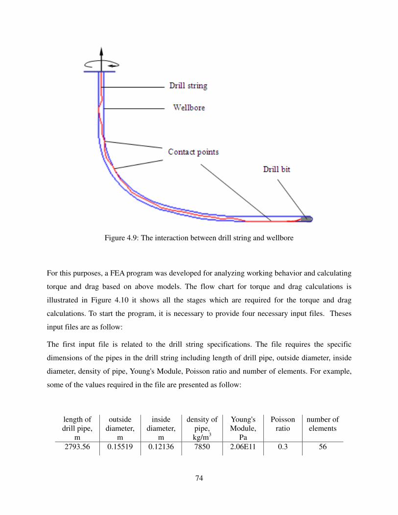
74
Figure 4.9: The interaction between drill string and wellbore
For this purposes, a FEA program was developed for analyzing working behavior and calculating
torque and drag based on above models. The flow chart for torque and drag calculations is
illustrated in Figure 4.10 it shows all the stages which are required for the torque and drag
calculations. To start the program, it is necessary to provide four necessary input files. Theses
input files are as follow:
The first input file is related to the drill string specifications. The file requires the specific
dimensions of the pipes in the drill string including length of drill pipe, outside diameter, inside
diameter, density of pipe, Young's Module, Poisson ratio and number of elements. For example,
some of the values required in the file are presented as follow:
length of drill pipe,
m
outside diameter,
m
inside diameter,
m
density of pipe, kg/m3
Young's Module,
Pa
Poisson ratio
number of elements
2793.56 0.15519 0.12136 7850 2.06E11 0.3 56

75
The second file is the wellbore geometry file which includes measured depth, inclination,
azimuth, friction coefficient related to cased and open hole as well as the buoyancy factor which
could change during different operation by changing the drilling fluid density. The following is
an example of values for the well geometry file at a specific measured depth.
measured depth, m inclination, rad azimuth, rad friction factor Buoyancy factor
528.83 0.0105 2.916 0.3 0.8675
The third input file is for controlling the program and is called the control parameters file. The
parameters include, time step, Wilson-theta value, total number of steps, wellbore clearance and
hook stiffness. As an example, some values are listed for the control parameters below:
time step,s theta total steps bit mass, kg clearance, m stiffness, N.m2
0.005 1.5 2000 30 0.015 8.06E6
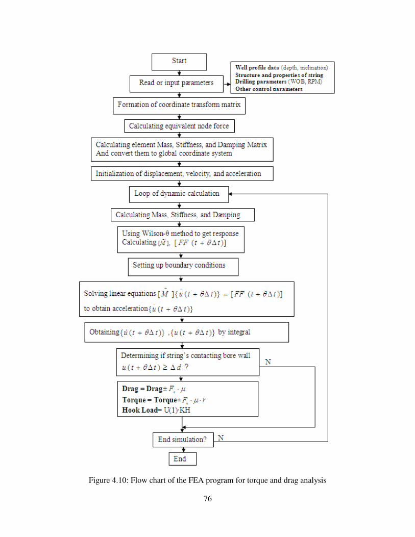
76
Figure 4.10: Flow chart of the FEA program for torque and drag analysis
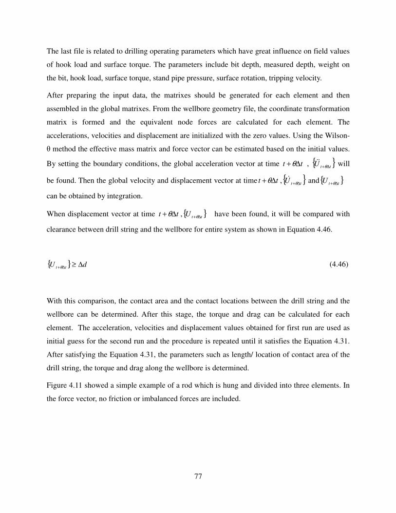
77
The last file is related to drilling operating parameters which have great influence on field values
of hook load and surface torque. The parameters include bit depth, measured depth, weight on
the bit, hook load, surface torque, stand pipe pressure, surface rotation, tripping velocity.
After preparing the input data, the matrixes should be generated for each element and then
assembled in the global matrixes. From the wellbore geometry file, the coordinate transformation
matrix is formed and the equivalent node forces are calculated for each element. The
accelerations, velocities and displacement are initialized with the zero values. Using the Wilson-
θ method the effective mass matrix and force vector can be estimated based on the initial values.
By setting the boundary conditions, the global acceleration vector at time tt ∆+θ , ttU ∆+θ&& will
be found. Then the global velocity and displacement vector at time tt ∆+θ , ttU ∆+θ& and ttU ∆+θ
can be obtained by integration.
When displacement vector at time tt ∆+θ , ttU ∆+θ have been found, it will be compared with
clearance between drill string and the wellbore for entire system as shown in Equation 4.46.
dU tt ∆≥∆+θ (4.46)
With this comparison, the contact area and the contact locations between the drill string and the
wellbore can be determined. After this stage, the torque and drag can be calculated for each
element. The acceleration, velocities and displacement values obtained for first run are used as
initial guess for the second run and the procedure is repeated until it satisfies the Equation 4.31.
After satisfying the Equation 4.31, the parameters such as length/ location of contact area of the
drill string, the torque and drag along the wellbore is determined.
Figure 4.11 showed a simple example of a rod which is hung and divided into three elements. In
the force vector, no friction or imbalanced forces are included.

78
Figure 4.11: FEA of a rod with one end fixed
The rod is divided into 3 elements, which gives four nodes. The comparison between the exact
value and the FEA is shown in Table 4.1. The difference between the exact value and FEA is due
to the approximation nature of the finite element method.
Table 4.1: Comparison of Exact value with FEA of the rod
Nodes Exact value, N FEA, N U1 0 0 U2 0.563835 0.553915 U3 0.752136 0.726339 U5 0.835903 0.817175
Another example in which the drill string is located in a vertical well is shown in Figure 4.12.
The drill string is hung with a hook and rotates with a constant speed at the surface. The bottom
of the string is applied with a reactive load and the weight on the bit as 525 kN. Using the FEA
program, the hook load and displacements including rotation at any node can be obtained.
The input parameters are as follow:
n =60 rpm
ε=2πn/60=6.28(rad/s)
total elements=200
length of the string=2000m

79
total weight of the string=659.73KN
WOB=525KN
Figure 4.12: FEA of vertical well drilling
The calculated parameters using the FEA are as follow:
hook load=251.56KN
actual value=659.73-525=235.73
relative error= (251.56-235.73)/235.73=2.87%
The error is acceptable and refers to the nature of finite element solution which is an
approximation as well as the stiffness of a virtual spring as taken for hook assembly.
Figure 4.13 shows the axial displacement at four different nodal locations such as surface (hook),
700 m, 1400 m, and bottom (bit). Figure 4.13 shows by increasing the depth, the displacements
will be decreased. For the displacement of the hook at the surface, it can be seen that the
displacement is less than those at 700 m and 1400 m due to larger stiffness coefficient of the
hook than drill string at 700 and 1400 m.

80
Figure 4.13: The axial displacement of four different locations
Figure 4.14 shows the rotary speed at three different locations 700m, 1400m, and drill bit. At the
beginning, the rotary speed of the drill bit responds slower and the speed at the 700m location
responses faster as shown in the plot. This delay is due to transmission of torsion from the
surface to the bit which is proportional to the distance between the surface and point of interest.
Here, the points of interest are 700 m, 1400 m and the bit.
Figure 4.14: The rotary speed at three different locations
81
CHAPTER FIVE: MODELING CONSIDERATIONS
Friction coefficient plays an important role in torque and drag modeling calculations and may in
some cases be a cause of confusion. It is defined as the roughness between the drill string and
wellbore wall, but there are always some unwanted contributions that influence the true value of
measured torque and drag. In this chapter, these effects have been investigated to get a more
reasonable value for the friction coefficient for real time torque and drag analysis.
5.1 Buoyancy
The principle of Archimedes is used in buoyancy calculations. The principle says when a body is
submerged into a fluid; the buoyancy force is equal to the weight of displaced fluid. Aadnoy et
al. (2010) showed the drill string tension in a wellbore when filled with a drilling fluid is the unit
pipe weight w multiplied by the buoyancy factor β. Equation 5.1 is valid for vertical and deviated
boreholes if the inside and outside of the pipe are submerged into the same fluid.
pipe
mud
ρ
ρβ −= 1 (5.1)
Equation 5.1 gives a good estimation of buoyancy factor when the drilling fluids are
incompressible and the effect of temperature and cutting concentration can be ignored. This
equation can be used for over-balanced drilling operations unless tripping in, which is discussed
in following paragraph.
If there is a fluid density difference between the inside of the drill string and in the annulus, like
during cementing and tripping in operations, the following equation should be used for local
buoyancy factor calculations, Aadnoy et al., (2006).
( )22
22
1iopipe
iioo
dd
dd
−
−−=
ρ
ρρβ (5.2)
82
Equation 5.2 can calculate the buoyancy factor locally for each drill string element. In tripping-in
operations, during running-in, the annulus is completely full but the inside of the string is
initially empty. The reason why the drill string is empty is because the drilling crew does not
typically fill the drill string during connections. Considering the collapse pressure of drill string
and possible risk of blowout, the crew will typically schedule to fill the drill string after running-
in every few hundred meters. This means the drill string will be partially full for a period of time
and then will be completely full after running the desired length of drill string. When the drill
string is full of mud the Equation 5.2 will turn into Equation 5.1 but when it is partially full and
some portion of drill string is empty the Equation 5.2 will be used.
For tripping out, the mud level in the annulus does not drop quickly due to large surface area of
annulus. Also the drilling crew fills the hole up using an auxiliary pump through fill-up line as a
part of their routine jobs on the rig for having sufficient hydrostatic pressure for kick prevention.
Therefore, the changes in buoyancy factor during tripping out are negligible.
5.1.1 Underbalanced Drilling
For underbalanced drilling specially in foam and aerated mud drilling, the density of the drilling
fluid is not constant and changes along the circulating system. Drilling fluids have different
compositions inside and outside the drill string. Inside the drill string, the drilling fluid is only a
mixture of incompressible fluid and injected gas which flows under a two-phase condition. In the
annulus the generated drill cuttings and formation influx fluid which may be a liquid or a gas,
will be added and the fluid mixture and the mixture is now three phases. In this condition, the
density depends on the following parameters:
injected gas or air flow rate into circulating system
pressure along drill string and annulus
average temperature
rate of penetration
rate of influx
nature of influx

83
back pressure
bottom hole pressure
All aforementioned parameters are subjected to change and should be recorded as real-time data
during different underbalanced operations and then considered in the buoyancy calculations. In
the following paragraph, the practical way of considering these parameters in the buoyancy
calculations is discussed.
Equation 5.2 is used to calculate the buoyancy factor at any measured depth. This equation will
give the local buoyancy factor and it should be multiplied by the unit weight of each element at
that particular depth. To calculate the local buoyancy factor, it is required to have density of
drilling fluid inside and outside of drill string versus measured depth.
Density inside Drill string
In aerated mud drilling, drilling fluids which are essentially incompressible are injected with
atmospheric air or other gases. To develop a practical equation for the drilling fluid inside the
drill string, assume the following (Lyons, et. al., 2009):
The compressible gases could be approximated by ideal gas law.
The mixture of compressed gas and incompressible drilling fluid is uniform and
homogeneous.
Considering these assumptions, the general equation for density of the mixture inside the drill
string can be written as follow
mudgas
mudgas
mixQQ
mm
+
+=
&&
ρ (5.3)

84
where m& and Q represent mass and volumetric flow rate respectively.
Lyons, et. al., (2009) presented the Equation 5.4 for calculation of mixture density inside the drill
string. “g” and “m” represents gas and drilling mud in this two phase system.
mg
g
aveg
mmg
ge
gg
n
mix
QQT
T
P
P
QQTR
SP
g+×
+
×=
γ
ρ1
(5.4)
Where
gn: acceleration gravity, 9.8066 m/sec2
Pg: absolute atmospheric pressure, N/m2
S: specific gravity
γ: specific weight, N/m3
Re: engineering gas constant, 29.31 N.m/N.K
Tg: absolute atmospheric temperature, K
P: pressure at any depth, N/m2
Tave: absolute average temperature, K
Density inside Annulus
Drilling fluid in the annulus is subjected to change. The generated drilling cuttings and influx is
added to the drilling fluid which comes out of bit nozzles. The drilling fluid no longer is two-
phase and the solid phase will be added to it. The density equation can be written for the annulus
as follow:
85
luxsolidmudgas
luxsolidmudgas
mixQQQQ
mmmm
inf
inf
+++
+++=
&&&&ρ (5.5)
In comparison with volumetric flow rate of gas and liquid, the volumetric flow rate of drilling
cuttings is negligible. But due to much higher density of drilling cuttings compared to gas and
liquid, the mass flow rate of solid should be considered in the density calculation (Lyons, et. al.,
2009).
( )
0
7.24
1
4
22
≅
×××=×=
solid
w
n
solidsolid
Q
ROPDg
ROPDm γπ
ρπ
& (5.6)
For influx, there are two scenarios which should be distinguished for different cases. The influx
could be gas or liquid, thus different equations should be used to calculate their mass and
volumetric flow rates. For the liquid case, influx could be saline or liquid hydrocarbons which
could be assumed to be incompressible. The mass and volumetric flow rate will not change by
change in pressure and temperature as shown in Equation 5.7.
( ) ( ) ( )luxll
n
luxllluxl Qg
Qminfinfinf
1γρ ×=×=& (5.7)
If the influx is gas, the same formula for injected compressed gas will be used to calculate its
mass and volumetric flow rate. Equations 5.8 and 5.9 can be written in following formats for
liquid and gas influx. For liquid and gas influxes, Lyons, et. al., (2009) presented the followings:

86
( )
( )luxlmg
g
aveg
luxllwmmg
ge
gg
n
mix
QQQT
T
P
P
QROPDQQTR
SP
ginf
inf
2 )7.2(41
++×
+×++
×=
γγπ
γ
ρ (5.8)
and
lux
g
g
aveg
mg
g
aveg
lux
g
ge
gg
wmmg
ge
gg
n
mix
QT
T
P
PQQ
T
T
P
P
QTR
SPROPDQQ
TR
SP
g
inf
inf
2 )7.2(41
×++×
+×++
×=
γπ
γ
ρ (5.9)
5.2 Viscous Drag Force
The viscous drag force is the effect of the moving pipe on the annular mud velocity. The moving
pipe walls transport mud in the direction of motion of the pipe, and at the same time the volume
of the pipe displaces mud in an opposite direction of the pipe’s motion. The annular mud
velocity to calculate viscous pressure gradient depends on factors such as:
the nature of the fluid (whether Newtonian or non-Newtonian)
flow regime (laminar or turbulent)
the pipe velocity
open ended or close ended string (check valve (float) present in the string)
Maidla and Wojtanowicz, (1987, a) showed the hydrodynamic viscous force effect is considered
by calculating surge or swab pressure associated with drilling mud flow caused by pipe
movement in the wellbore. They presented a viscous pressure gradient for each pipe element.
The calculation procedure for the viscous pressure gradient is based on the theory of viscous
drag force for Bingham-plastic and Power-Law fluids in the wellbore. These equations presented
by Maidla and Wojtanowicz, (1987, a) are applicable only for close end strings. The calculation
procedure includes the following steps:

87
Step 1: Calculation of mud clinging constant, Cc
The value of effective mud velocity due to the moving pipe wall is related to the pipe velocity
by proportionality constant cC . The value of cC depends upon the ratio of pipe and hole
diameters, δ .
For the laminar flow
δδ
δδδ
ln)1(2
1ln22
22
−
−−=cC (5.10)
and for the turbulent flow
2
24
1
1
δ
δδ
δδ
−
−+
+
=cC (5.11)
Step 2: Calculation of the average effective annular velocity, aev
It is the mud velocity that produces the viscous drag component of surge pressure. Its frame of
references is the wellbore wall which was defined by Burckhardt, (1961).
+
−×= cpae Cvv
2
2
1 δ
δ (5.12)
where
Vp: pipe velocity, m/sec

88
Step 3: Calculation of Reynolds number ReN for annular flow:
The Reynolds number can be calculated using Equation 5.13.
PV
dDvN ae )(
Re
−=
ρ (5.13)
Where
PV: plastic viscosity, N.sec/m2
For 2100Re ≤N and 2100Re >N the flow is laminar and turbulent respectively.
Step 5: Calculation of the friction factor
For smooth pipe and a Reynolds numbers less than105, a straight line approximation of the
Colebrook function for Bingham-plastic fluid yields accurate friction factor presented by
Bourgoyne, et. al., (2001). It is known as the fanning friction factor. The fanning equations for
Laminar flow are:
Re
16
Nf = (5.14)
For turbulent flow:
25.0
Re
0791.0
Nf = (5.15)
Step 5: Calculation of the viscous pressure gradients, ∆P/∆L
89
Viscous pressure gradient for Bingham-plastic model was presented by Burckhardt, (1961).
)(
2
dD
fv
L
P ae
−=
∆
∆ ρ (5.16)
After calculating viscous pressure gradient, the hydrodynamic viscous drag force can be
calculated by Equation 5.17:
∑=
∆∆
∆=
n
i
iiiD dLL
PF
1
2)(
4
π (5.17)
The calculated viscous drag force for entire drill string should be added or subtracted to the
calculated hook load during tripping out and in respectively to get a more reasonable friction
coefficient.
5.3 Contact Surface
Maidla and Wojtanowicz, (1987, b) presented contact surface correction factor to consider in
drag calculations. The correction factor, Cs, represents an effect of the contact surface between
the pipe and the wellbore due to larger curve surface contact are. They showed that when a
cylinder with outer diameter d moves through a pipe with the inner diameter D with applying a
normal force FN, the drag force will be as follow:
NFFF ××= µπ
4 (5.18)

90
Equation 5.18 shows that the real drag force for curve contact surface is 4/π times larger than a
flat contact surface. In this case, the correction factor is 4/π. In case of pipe string and wellbore,
the string outer diameter is smaller than the wellbore diameter. The drag force can be written as:
NS FCFF ××= µ (5.19)
This correction factor values varying between 1 and 4/π are dependent upon contact surface
angle γ which vary between o0 and o90 . Contact surface angle γi mainly depends on wellbore
and string outer diameters. Maidla and Wojtanowicz, (1987, a) showed how contact surface
effect can be calculated for each point using Equation 5.20.
1)14
(2
+−=π
γπ
iiCs (5.20)
For calculating the contact surface angle, the following procedure presented by Maidla and
Wojtanowicz, (1987, a) should be used:
)2
2tan(
iii
ii
dDY
XArc
+−=γ (5.21)
Where:
)2(
)2(
4
1222
iii
iiiii
iddD
ddDDdY
∆+−
∆+−+−×= (5.22)

91
2
1
224
2
1iii YdX −×= (5.23)
i
i
i
i
iiii
i
it
d
R
Fww
Ed ×
++×=∆ −2
1
212 )sin()cos(24
αβϕβπ
(5.24)
The values of ∆di are negligible due to big value of modulus elasticity of steel which is2×1011 Pa.
Its ignorance will not effect on value of Csi. If the ∆di is ignored, Csi will be only the function of
wellbore diameter and string outer diameter and can be rewritten as follow:
( )11
4tan
2 2
122
+
−×
−
×=ππ i
iii
d
dDArcCs (5.25)
To include contact surface effect in the torque and drag equations, it should be multiplied by the
friction coefficient. If this effect is ignored in the calculations a bigger friction coefficient should
be used to match modeling data with measured data.
The important application of this factor is monitoring the wellbore conditions during tripping in
and out of the drill string. When BHA, which has greater diameter than drillpipe, passes through
some section with smaller diameter, the overall friction coefficient will increase due to contact
surface effect and this effect can be seen in real time analysis.
5.4 Sheave Friction
On the rig, the maximum load of the drill string weight and friction is applied on the hook. For
measuring hook load, a hydraulic load cell or a strain gage “turtle” is attached to the dead line.
The hook load displayed by the weight indicator which is assumed to be equal to the number of
lines between blocks N, multiplies by dead line tension dlF .

92
NFHL dl×= (5.26)
Equation 5.26 is accepted industry method to calculate the hook load. It does not account for
sheave friction and does not consider the difference between static and dynamic conditions. Luke
and Juvkam-Wold, (1993) showed that true hook load depends on sheave friction and direction
of block movement. They proved that true line tension from dead-line tension readings does not
reside with the use of deadline readings, but with how these tension readings can be used.
When tripping out, the tension gradually reduced from the fast line to the dead line. In this way,
the fast line would have the highest tension and dead line would have the lowest tension. It
means that the indicator will display low when the drill string is being pulled out. When tripping
in, the highest line tension is the dead line and the lowest tension is in the fast line. It results in
high readings by weight indicator during the running of the drill string in the hole.
Dangerfield, (1987) made a mathematical analysis of the frictional resistance on the hoisting
system. In his analysis, he proposed that two type of deadline sheaves existed: active and
inactive. The active deadline sheave is the sheave in crown block which the dead line passes over
and back to the traveling block. It is free to rotate. It is also known as friction sheave due to
differential between the tensions in the lines on either side of the sheave. For the inactive dead
line sheave which is known as frictionless sheave, the tensions in the lines on both sides of the
sheave are the same.
The following equations presented by Luke and Juvkam-Wold, (1993) include direction of drill
string movement and type of deadline sheave for true hook load prediction. For an inactive
(frictionless) deadline sheave, when tripping the drill string out, the hook load can be calculated
as follow,
( )[ ]( )1
/11
−
−×=
e
eeFHL
N
dl (5.27)
93
When tripping in:
( )e
eFHL
N
dl−
−×=
1
)1( (5.28)
For active (friction) dead line sheave, when pulling the drill string out, the hook load will be as
follow:
( )( ) N
N
dlee
eFHL
−
−×=
1
1 (5.29)
For tripping drill string in, the hook load is:
( )e
eeFHL
N
dl−
−×=
1
)1( (5.30)
Luke and Juvkam-Wold (1993) showed the average sheave efficiency e ranged from 96% to
99% for hook load estimation. For sheave efficiency determination, it is required to raise and
lower a certain weight such as drillpipe joint using the hoisting assembly and record the
measured value with actual weight to estimate sheave efficiency.
5.5 Hydraulic Vibrations
Rapid shut down of a control valve or stopping of a pump produces excess pressure in a tubular.
Hydraulic transient as used more recently, refers to pressure fluctuations caused by a sudden
change in the flow rate. Barakat, (2005) showed that when the fluid flow is stopped instantly, it
results in a pressure increase which propagates at pressure wave speed in the fluid through the

94
fluid which causes radial expansion of the tubular wall. Due to this radial expansion, the pipe
shortens behind and elongates in front of pressure rise. The application of hydraulic transient
studies will be discussed further in following sections.
5.5.1 Agitator
Based on hydraulic transient, a dynamic excitation tool, Agitator, has been designed by National
Oilwell Varco, (2008). Agitator smoothly oscillates the drill string to substantially reduce axial
friction force. This means improved weight transfer and reduced stick-slip and reduced stick-slip
in all modes of drilling. It provides this facility to increase the length of a horizontal section by
breaking the axial friction force as shown in Figure 5.1. In the figure the dynamic and static
friction refer the conditions with and without using agitator in drill string.
Figure 5.1: Effect of hydraulic vibration on axial friction force (Agitator Tool Handbook, 2008)
The Agitator system relies on three main sections.
Power
Valve and bearing

95
Shock tool
The power section is short positive displacement motor which drives the valve section producing
pressure pulses which in turn activate the shock tool. It is the axial motion of the shock tool
which breaks static friction and converts it to dynamic.
Figure 5.2 shows the axial load along drill string when there is no agitator in the string. During
long reach horizontal drilling, before and after build-up sections, the helical buckling is more
probable to happen due to high compressive load as a result of axial friction and weight on the
bit. This helical buckling causes additional axial friction force and lower weight on the bit.
Figure 5.2: The tension-compression and axial friction forces along drill string without agitator
(Agitator Tool Handbook, 2008)
Using an agitator in drill string as shown in Figure 5.3 mitigates the chance of helical buckling
and reduces axial friction force along drill string. This reduction in axial friction force will
improve the amount of weight on the bit in drill string slack off.

96
Figure 5.3: The tension-compression and axial friction forces along drill string using agitator
(Agitator Tool Handbook, 2008)
Figure 5.4 (a) shows a set of field data related to a wiper trip and the drilling operations which
did not use agitator. The drill string slacking off is between 18 to 27 daN and multiple pressure
spikes can be seen. For the field case with the agitator as shown in Figure 5.4 (b) a constant slack
off weight can be seen. The drill string slacking off value changes between 15 to 18 daN and no
big pressure spikes is seen any more. Overall pressure has been increased as much as 3500 kPa
due to pressure drop across agitator.

97
(a) (b)
Figure 5.4: Effect of using agitator on drilling parameters (Agitator Tool Handbook, 2008)
5.5.2 Surface Pressure Applied inside Drill string
Aadnoy and Kaarstad, (2006) showed effect of surface pressure on hook load measurements.
They showed that the axial tension increases due to the inside applied surface pressure which is
equal to the pressure increment multiplied by inner cross sectional area of drill string. The
pressures in the drill string and annulus while applying surface pressure inside drill string e.g.
during drilling are as follow:
lossgdrillstrinsurfacechydrostatigdrillstrin PPPP )(∆−+= (5.31)

98
and
lossannulusbitgdrillstrinsurfacechydrostatiannulus PPPPPP )( ∆+∆+∆−+= (5.32)
Equations 5.31, 5.32 can be written for the surface drill string element which received maximum
pressure and minimum pressure for inside and outside respectively. The pressure inside
drillstring is taken as stand pipe pressure, SPP.
SPPPPP surfacegdrillstrinannulus === ,0 (5.33)
Equation 5.34 can be used to estimate the additional tensional force due to inside drilling fluid
pressure which should be added to the hook load calculations during friction analysis.
2
4
1IDSPPFp ××= π (5.34)
5.6 Buckling
A tubular can be buckled in any wellbore, but the axial compressive load to initiate buckling is
different for different sections such as vertical, curved and horizontal as shown by Wu and
Juvkam-Wold, (1995). The buckling may cause problems during drilling and casing running
which may not transfer sufficient weight on the bit or to allow the casing to seat in right place.
5.6.1 Buckling Criteria
In a real time application, it is necessary to monitor the compressive load along drill string to
find the type and beginning point and length of buckling and consider them in torque and drag
analysis.

99
In a horizontal section, the tubulars are in compression due to axial friction, weight on the bit,
and/or load on the packer. When the axial compressive load exceeds the following critical load,
the tubular will buckle sinusoidally (Wu and Juvkam-Wold, 1993) as:
2
1
)/(2 rwEIFCr β×=
(5.35)
For an inclined wellbore the Equation 5.35 can be written as follow:
2
1
)/sin(2 rwEIFCr αβ ××=
(5.36)
The effect of sinusoidal buckling on the axial friction force is negligible and the sinusoidal
tubular is treated the same as a straight one. When the compressive load exceeds the following
loads the helical buckling will happen in the horizontal and inclined wellbores as discussed by
Aadnoy, (2006).
Crhel FF ×−= )122( (5.37)
In vertical section, the tubular is easily buckled which adds some considerable axial friction
force. Equation 5.38 calculates the critical load for sinusoidal buckling which was presented by
Wu and Juvkam-Wold, (1993).
3
1
2 ))((55.2 wEIFCr β××=
(5.38)

100
The helical buckling load is about 2.2 times as large as the sinusoidal buckling load in vertical
wellbores as shown in Equation 5.39 presented by Wu and Juvkam-Wold, (1993).
Crhel FF ×= 18.2 (5.39)
5.6.2 Axial Force along Drill string
The axial load distribution will be changed when a tubular is buckled helically. When the drill
string or casing buckles in a wellbore, an additional friction force will be generated. This
additional friction force should be considered while estimating downhole weight on the bit. Also,
this helical buckling may limit us sooner for extended reach well drilling.
In horizontal sections, when a tubular is running without helical buckling, the compressive load
increases linearly due to axial friction caused by tubular weight as shown in Figure 5.5. Equation
5.40 shows the linear relationship between compressive load and length of tubular in horizontal
section when no buckling happens.
LwFF ∆×+= µβ12 (5.40)
Where ∆L is the length of a non-buckled element and F1 is the compressive force at the bottom
of the element.
An additional friction force is generated due to the wellbore confinement to the helical buckling
which should be considered in torque and drag analysis. Wu and Juvkam-Wold, (1993) showed
that this additional friction force increases with the rate of square of axial compressive load. The
axial compressive load distribution becomes nonlinear as shown in Figure 5.5 and has to be
calculated by Equation 5.41 as follow:

101
( ) ( )[ ] ( )[ ]
+∆×= 2
1
12
1
2
1
2 4/arctan4/tan/2 wEIrFEIwrLrwEIF ββµβ
(5.41)
Where, ∆L is now measured for the element in the helically buckled portion of the tubular.
For inclined and curved sections, Equation 5.41 can be written as:
( ) ( )[ ] ( )[ ]
+∆×= 2
1
12
1
2
1
2 sin4/arctan4/sintan/sin2 αβαβµαβ wEIrFEIwrLrwEIF
(5.42)
Figure 5.5: Schematic of tubular buckling in horizontal section
Theoretically, there is no axial friction force in vertical wellbore and compressive force along
drill string can be written as:
102
LwFF ∆×−= β12
(5.43)
Where, L∆ is measured element along the drill string and upward and F1 is the axial
compressive force at the bottom of the element. Wu and Juvkam-Wold, (1993) presented
Equation 5.44 to calculate the compressive axial load distribution when helical buckling happens
and causes the axial friction force in a vertical wellbore.
( ) ( )[ ] ( )[ ]
+×∆−= 2
1
12
1
2
1
2 4/arctan4/tanh)/(2 wEIrFhEIwrLrwEIF βµβµµβ
(5.44)
Where, L∆ is measured for helically buckled portion of tubular in vertical wellbore.
For torque increment during helical buckling, it should be mentioned when helical buckling
happens, the pipe rotation is brutal and it should be avoided. It is a routine practice in the field
when chance of helical buckling is high during oriented drilling, the weight on the bit should be
released and then surface rotation should be started.
5.7 Off/On Bottom Data Selection
It is crucial to select the correct off and on bottom calibration data points for torque and drag
analysis during drilling operations. When the drill string is lowered for further drilling, there are
different values for the hook load which can be related to pump off force, tight hole, interaction
between stabilizer and the wellbore, cutting accumulation etc. It is very important to recognize
when the drill bit touch the bottom of the hole and interact with the formation.
When the bit interacts with the formation, an increase in stand pipe pressure can be observed due
to increase in differential pressure across the downhole motor if a motor is used. The interaction
cause more torque at the bit is provided by the downhole motor. The generated torque in
downhole motor requires more pressure drop which results an increase in stand pipe pressure.
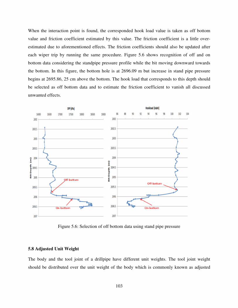
103
When the interaction point is found, the corresponded hook load value is taken as off bottom
value and friction coefficient estimated by this value. The friction coefficient is a little over-
estimated due to aforementioned effects. The friction coefficients should also be updated after
each wiper trip by running the same procedure. Figure 5.6 shows recognition of off and on
bottom data considering the standpipe pressure profile while the bit moving downward towards
the bottom. In this figure, the bottom hole is at 2696.09 m but increase in stand pipe pressure
begins at 2695.86, 25 cm above the bottom. The hook load that corresponds to this depth should
be selected as off bottom data and to estimate the friction coefficient to vanish all discussed
unwanted effects.
Figure 5.6: Selection of off bottom data using stand pipe pressure
5.8 Adjusted Unit Weight
The body and the tool joint of a drillpipe have different unit weights. The tool joint weight
should be distributed over the unit weight of the body which is commonly known as adjusted

104
unit weight. The adjusted unit weight values should be given by manufacturers so more accurate
values can be used in torque and drag software’s and real time analysis.
Also, the drill string wears after being used for a period of time. The drill pipe should be
classified according to API classification as shown in Table 5.2 presented by Samuel, (2010).
The corrected outside drill pipe diameter is calculated as the following.
)1( cIDdcdCorrected −×+×=
(5.58)
Where c is the drillpipe class multiplier based on API classification. Table 5.1 lists the pipe class
multipliers for various classes of pipe.
Where c and ID are the drillpipe class multiplier based on API classification and inner diameter
of the pipe respectively. Table 5.1 lists the pipe class multipliers for various classes of pipe:
Table 5.1: The multipliers for various classes of pipes (Samuel, 2010)
NO. Pipe Class Class Multiplier, c
1 N: new 1.000
2 C: critical 0.875
3 P: premium 0.800
5 2: class II 0.700
5 3: class III 0.650
The following example shows how the class of the drillpipe class affects the original unit weight.
Coiled tubing has been selected for this example due to the uniform nature of the tubing without
any tool joints.

105
New:
ftlbUW
inID
inOD
c
newclass
/7.3
063.2
375.2
000.1
=
=
=
=
=
If the class of pipe changed to premium class:
ftlbUW
inID
inOD
c
premiumclass
Corrected
Corrected
/92.2
063.2
3126.2
800.0
=
=
=
=
=

106
CHAPTER SIX: TECHNICAL RESULTS AND DISCUSSION
This chapter includes the field data analysis for the verification of the new models (analytical
and finite element) discussed in the previous chapters. Some field cases have been selected from
Canadian and North Sea wells for further discussion and evaluations. The field cases
demonstrate the challenges during different operations such as drilling, tripping in/out, and
reaming/back reaming. Also, a new developed method based on the friction models is presented
to estimate the down hole weight on bit (DWOB) for directional drilling applications from
surface hook load measurements. The application of this new DWOB method in an autodriller
system is discussed in detail.
6.1 Analytical Modeling of a Two-Dimensional Well
The record of this horizontal well field case was extracted in January 2009 from an onshore rig
in Alberta, Canada. The horizontal departure and vertical section of the well are shown in Figure
6.1.
Figure 6.1: Geometry of the horizontal well in Alberta, Canada

107
A 9 5/8 inch surface casing string was run to the depth of 2090 ft. An intermediate 7 inch casing
was set at 7500 ft. To reach the target a 6 1/8 inch bit was used to drill the horizontal section.
This example will demonstrate the application of the model for tripping the drill string out. The
drill string total length is 10995 ft, which is shown in Figure 6.2. In this horizontal well, the drill
string must be forced into the wellbore. Here, the 4 inch heavy weight drill pipes were placed in
the vertical section to provide sufficient weight to push the drill string into the horizontal section.
The entire drill string in the horizontal section is compressed during drilling. The adjusted weight
for the 4 inch drill pipe and 4 inch heavy weight drill pipe are 17.71 lb/ft and 29.92 lb/ft,
respectively. The adjusted diameter for the drillpipe and heavy weight drillpipe is 4.1 inch. The
well is filled with a drilling fluid with a weight of 8.9 lb/gallon. For this well, there is no change
in the well azimuth. As a result, the dogleg change for this well is that of the inclination.
Figure 6.2: Drill string configuration for the horizontal well

108
6.1 .1 Tripping Out
Figure 6.3 shows the measured hook loads while tripping out. The measured hook load values
are a function of drill string length, well geometry, drill string configuration and wellbore
conditions. Different wellbore geometries and drill string configurations in the vertical sections
show different measured hook load trends. Also, Figure 6.3 shows the hook load measurements
when the entire drill string weight is on the slips during connection times. Hook load
measurements during connection time represent the weight of the hoisting assembly at surface
without a precise calibration. It is noted that the data recording commenced when the bit depth
was 740 ft.
Figure 6.3: Measured hook load versus measured depth during tripping out
The friction coefficients usually vary from 0.1 to 0.4 to match the normal field data. Figure 6.4
illustrates a comparison between the measured and calculated hook load values for different

109
friction coefficients. This comparison shows that even with a low value of the friction coefficient
(e.g., friction coefficient of 0.1), there is still a maximum of 6 percent deviation from the field
data at the depth of 7700 ft.
Figure 6.4: Comparison between the measured and calculated hook loads during tripping out
For quality control of the field data, the tripping data should be compared with the static weight
of the drill string. Here, the static weight means the weight of drill string when there is no
friction during drillstring movement. Figure 6.5 indicates that the measured hook loads have
smaller values than static weight data. The latter is impossible. The field data related to tripping
out should always be greater than static weight as the friction force between the drill string and
wellbore is added to the static weight of the drill string. It is noted that the hook load data have
been recorded based on Equation 5.26. This equation is the widely accepted industry method,
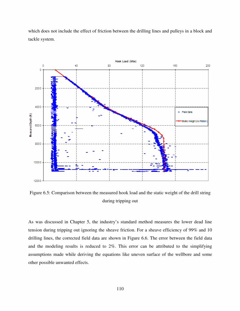
110
which does not include the effect of friction between the drilling lines and pulleys in a block and
tackle system.
Figure 6.5: Comparison between the measured hook load and the static weight of the drill string
during tripping out
As was discussed in Chapter 5, the industry’s standard method measures the lower dead line
tension during tripping out ignoring the sheave friction. For a sheave efficiency of 99% and 10
drilling lines, the corrected field data are shown in Figure 6.6. The error between the field data
and the modeling results is reduced to 2%. This error can be attributed to the simplifying
assumptions made while deriving the equations like uneven surface of the wellbore and some
other possible unwanted effects.
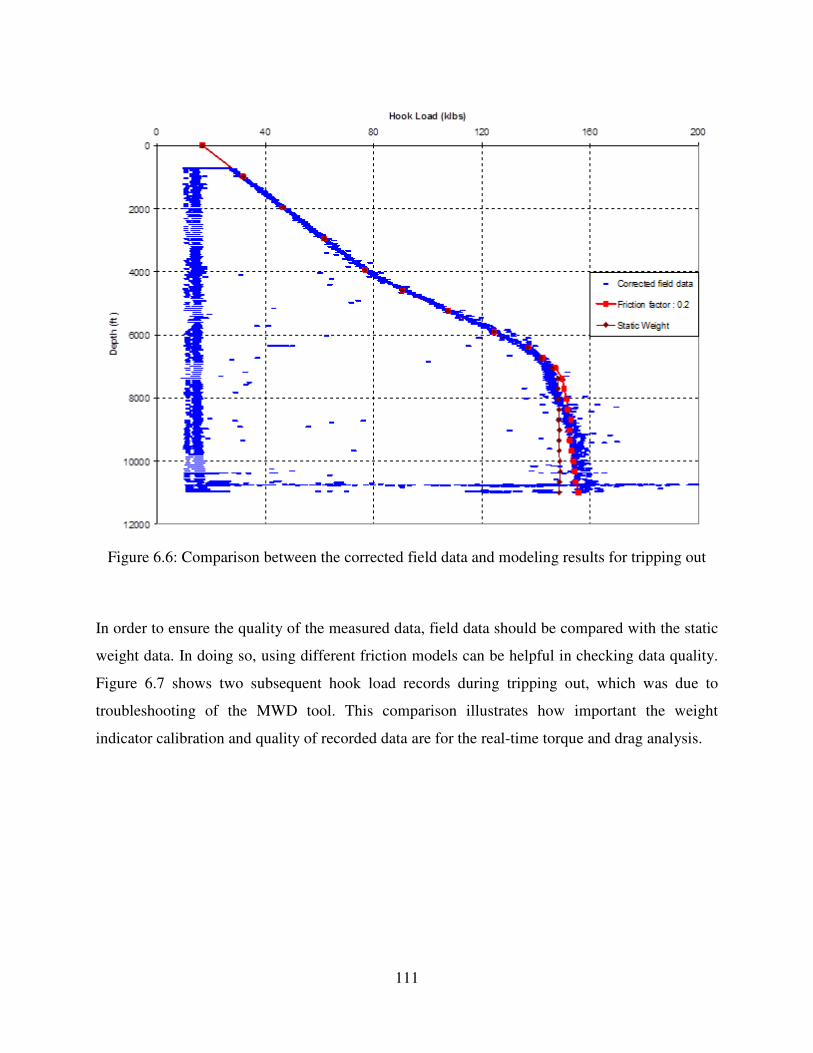
111
Figure 6.6: Comparison between the corrected field data and modeling results for tripping out
In order to ensure the quality of the measured data, field data should be compared with the static
weight data. In doing so, using different friction models can be helpful in checking data quality.
Figure 6.7 shows two subsequent hook load records during tripping out, which was due to
troubleshooting of the MWD tool. This comparison illustrates how important the weight
indicator calibration and quality of recorded data are for the real-time torque and drag analysis.

112
0
2000
4000
6000
8000
10000
0 40 80 120 160 200
Hook Load (klbs)
Me
as
ure
d D
ep
th (
ft)
Tripping out from 9360 ft
Tripping out from 9357 ft
Figure 6.7: Comparison between two subsequent measured hook loads during tripping out
6.1.2 Tripping In
Figure 6.8 shows hook load data for tripping in from the surface to depth of 10760 ft. The well
geometry is the same as that depicted in Figure 6.1. Similarly, the drill string configuration is
shown in Figure 6.2. The 4 inch heavy weight drill pipes were placed in the vertical section to
push the drill string into the horizontal section. The well is filled with the same drilling fluid with
a weight of 8.91 lb/gallon. The field data in Figure 6.8 were treated by assuming a sheave
efficiency of 99% for the 10 drilling lines between the pulleys.
Figure 6.8 shows a perfect match between the calculated and measured hook loads during
tripping in from the surface to a depth of 9100 ft. At the interval of 9100 to10400 ft, there is a big
reduction in measured hook loads, which is more than the expected values. This reduction can be
attributed to many factors such as the effect of buckling and ledging. These factors cause greater
friction coefficient for tripping in as opposed to that of tripping out. A remedy for minimizing
the adverse effects of buckling and ledging is the reaming and back reaming operations, which

113
make a smoother path with a lower friction coefficient. A hydraulic agitator can also be used to
release the compression force along the drill string in the horizontal section.
Figure 6.8: Comparison between measured and calculated hook loads while tripping in
A sensitivity analysis of the friction coefficient can be helpful in this scenario. In other words,
one should try to obtain an exact match between the measured and calculated hook load values
by inserting any value of the friction coefficient. Once the difference between two subsequent
friction coefficients gets very small, the drill string is then moving under normal conditions. On
the other hand, if the difference is considerable, a remedial action should be taken. Therefore,
sensitivity analysis of the friction coefficient could be helpful to predict any problem during
drilling operations. An example of finding trouble interval sections using sensitivity analysis of
friction coefficient during tripping in is given in Figure 6.9.

114
Figure 6.9: Sensitivity analysis of friction coefficient vs. measured depth while tripping in
6.1.3 Reaming/ Back Reaming
The surface torque is recorded during drilling with surface rotation, reaming and back reaming
operations. As it was discussed in tripping in, there was some resistance against the string
movement during running the drill string from the depth of 9100 ft to the target. To reduce this
resistance against axial movement, the drill string was rotated at the surface. Therefore, surface
torque was recorded during reaming and back reaming operations for this interval.
Figure 6.10 compares the measured and calculated surface torque during reaming and back
reaming operations. During the reaming operation, tripping and rotary speeds were 0.5 ft/sec and
55 rpm, respectively. The majority of the field data lie between the reaming and back reaming
calculated data, as shown in Figure 6.10. The measured torque data shows high fluctuations,
which reflect the nature of drill string rotation dynamics such as slip/stick, restoring moment,
torsional resistance and axial and lateral vibrations. It is usually difficult to compare the
calculated torque with the measured data with significant fluctuations. To make this comparison
easy, the measured data should be averaged over a short interval (see Figure 6.10).

115
Figure 6.10: Comparison between the measured and calculated surface torque during reaming
and back reaming
The first remedial action for over pull during tripping the drill string out is to rotate the drilling
string at surface. As it was discussed in Chapter 3, the model for the combined motions is used
to show the effect of rotation on the drag force reduction in the well. The drilling rig weight
indicators show a considerable difference between the drag force generated by tripping in/out
and reaming/back reaming operations. Figure 6.11 shows the effect of pipe rotation on the
calculated hook load during reaming and back reaming operations.

116
Figure 6.11: Effect of pipe rotation on the calculated hook load during tripping in/out
As was discussed in Chapter 3, the wellbore friction is divided into rotational and axial frictions.
By increasing either of them, the other one will decrease. For example, at a constant pipe surface
rotation speed, the torque values will decrease due to the increase of tripping speed, which leads
to an increase in axial friction. The effect of tripping speed on the calculated torque at a constant
rpm is shown in Figure 6.12.

117
Figure 6.12: Effect of tripping speed on the calculated torque during reaming operation
Additionally, if the pipe rotation speeds up at a constant tripping speed during the reaming
operation, it will result in higher torque values (see Figure 6.13). In this case, the major portion
of the friction force will be the rotational friction, which will trigger an decrease in the torque
along the drill string at the surface.
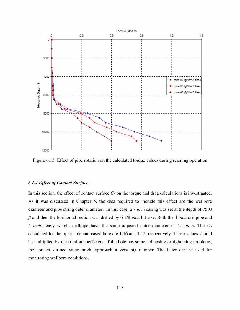
118
Figure 6.13: Effect of pipe rotation on the calculated torque values during reaming operation
6.1.4 Effect of Contact Surface
In this section, the effect of contact surface CS on the torque and drag calculations is investigated.
As it was discussed in Chapter 5, the data required to include this effect are the wellbore
diameter and pipe string outer diameter. In this case, a 7 inch casing was set at the depth of 7500
ft and then the horizontal section was drilled by 6 1/8 inch bit size. Both the 4 inch drillpipe and
4 inch heavy weight drillpipe have the same adjusted outer diameter of 4.1 inch. The Cs
calculated for the open hole and cased hole are 1.16 and 1.15, respectively. These values should
be multiplied by the friction coefficient. If the hole has some collapsing or tightening problems,
the contact surface value might approach a very big number. The latter can be used for
monitoring wellbore conditions.

119
Figure 6.14: Effect of contact surface on the calculated drag values during tripping in/out
Figure 6.14 shows the effect of contact surface on the calculated hook loads during tripping
in/out. When drill string is at the bottom of the well, the effect of contact surface on the hook
load value during tripping in/out is 0.3% and 1.5%, respectively. The effect of contact surface on
the torque calculations is more noticeable as the torque values pertinent to tripping in/out have
been increased to 5% and 20%, respectively. Figure 6.15 compares the torque values before and
after considering the effect of contact surface for torque calculations.

120
Figure 6.15: Effect of contact surface on the calculated torque values during tripping in/out
6.1.5 Effect of Hydrodynamic Viscous Force
Hydrodynamic viscous drag force is defined as the friction force between the pipe string and
drilling fluid, which creates a resistance against the pipe movement. This was comprehensively
discussed in Chapter 5. Viscous drag force depends on the drilling fluid properties, tripping
velocity, flow regime, pipe outer diameter and the wellbore diameter. Here, the drill string
configuration and the well specifications are the same as those given in the previous horizontal
well. For instance, the effect of drilling fluid rheological properties on the hydrodynamic viscous
drag force is shown in Figure 6.16.

121
Figure 6.16: Effect of mud rheology and clearance on the hydrodynamic viscous drag force
A higher viscous drilling fluid results in a higher viscous drag force. Also, this figure shows the
inverse relationship of clearance between the string and the wellbore and the viscous force.
Figure 6.16 can also be used to describe the effect of flow regime on the viscous drag force. At a
velocity of 1 ft/sec, the flow regime is laminar. When tripping speed is less than 4.5 ft/sec, the
flow regime is laminar in both cased and open holes. At a tripping speed of 5 ft/sec, due to
smaller clearance, the flow regime changes to transient flow in the open-hole section while it
remains laminar in the cased-hole section. Table 6.1 shows different flow regimes at different
tripping speeds.

122
Table 6.1: Flow regimes for different drill string position at different tripping speed
Tripping speed, ft/sec Drill string position Flow Regime
< 4.5 Cased Hole Laminar
< 4.5 Open Hole Laminar
5 Cased Hole Laminar
5 Open Hole Transient
Figure 6.17 shows how tripping speed affects the flow regime and the hydrodynamic viscous
drag force. By increasing tripping speed, the flow regime approaches turbulent mode. This
increases the viscous drag force drastically. Hydrodynamic viscous force should be added/
subtracted to/from the calculated hook load during tripping out/tripping in.
Figure 6.17: Effect of tripping speed and flow regime on hydrodynamic viscous drag force

123
6.2 Three Dimensional Well-Analytical Modeling
The well that has been considered for the friction analysis is located offshore in the North Sea.
The well starts vertically with a kick-off point of 350 m and a first build-up section to a depth of
1200 m. Then, the angle of this build-up section is held at 30º±2º inclination until a depth of
2750 m. At this depth, the second build-up section starts from an angle of 30º±2º to 90º. The
horizontal section starts from 4500 m to the final target. This well profile is a good candidate for
friction analysis as different sections of the well geometry (including straight inclined, curved
and horizontal sections) are present (see Figure 6.18). The 9 5/8” casing is set at a depth of 3207
m with an open-hole section to 5247 m.
Figure 6.18: Well geometry with casing shoe depths

124
6.2.1 Tripping out
Figure 6.19 shows the hook load values for the tripping out operation. The calculations started
from the bottom to the surface using 100 m elements. This calculation is repeated for different
friction coefficients. Two different friction coefficients are considered. First, a single value is
used for the friction coefficient for the entire well including the open and cased hole sections.
The friction factor value is changed stepwise as 0.2, 0.3 and 0.4. For the second case, different
friction factors are considered for the open-hole and cased-hole sections. The friction factor is
maintained for the cased hole at a constant value of 0.2; for the open-hole sections it is changed
to 0.2, 0.3 and 0.4. In this section, three models have been used for analysis. The Exxon model is
the model which developed by Johancsik in 1984. The Texas A&M model is the simple accepted
industry model which is modified by using the dogleg angle concepts instead of average
inclination between two subsequent survey data points.
As is shown in Figure 6.19, the three models (including the newly developed analytical model)
match the field data reasonably. However, the three models do not match the field data in a hump
existing at an interval of 2180 m to 3140 m. This section is the build-up section, which starts
with an inclination of 30º and ends at 55º. These three models cannot predict the local increase in
hook load due to several factors. One factor is the well geometry. In this interval there is a build-
up section with an angle of 25º over a 960 m interval. Once the three soft string models are
applied (all of which assume the pipe as a cable which completely contacts the borehole wall),
the estimation of friction force is inaccurate. This is allotted to the fact that in reality the drill
string should be considered as a stiff string that could tolerate a bending moment in either of the
bending sections. The other reason could be due to cuttings accumulation. It means that any time
that the pumps are off and cuttings begin to settle, the cuttings will not be stable until they land
in the lower part of the intermediate build-up section. In this section, the problem is that after
getting to the casing shoe (i.e., where there are already extra cuttings accumulated due to the
increased annular diameter), the well has been circulated, but only one bottoms-up. One bottoms-
up circulation will not remove the cuttings from a cased hole at these inclinations. Thus, after
one bottoms-up, the annulus is still full of cuttings. The result is an avalanche of cuttings down
onto the top of the BHA. Although this amount of cuttings is not enough to pack off the annulus,
it may be sufficient to increase the friction (as can be seen in first hump section).
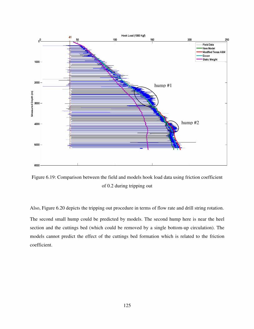
125
Figure 6.19: Comparison between the field and models hook load data using friction coefficient
of 0.2 during tripping out
Also, Figure 6.20 depicts the tripping out procedure in terms of flow rate and drill string rotation.
The second small hump could be predicted by models. The second hump here is near the heel
section and the cuttings bed (which could be removed by a single bottom-up circulation). The
models cannot predict the effect of the cuttings bed formation which is related to the friction
coefficient.
hump #2
hump #1

126
Figure 6.20: The tripping out procedure for North Sea candidate well in terms of flow rate and
drill string rotation
The torque plots for the comparison of the models prediction versus the field data are shown in
Figure 6.21. In this case, as the pipe is being pulled out of the hole, in most parts of the well
there is no torque because there is no pipe rotation. The drill string rotation from surface only
happens in two sections. A small section below the casing shoe as the hole wall is being reamed
and circulated to be cleaned. Another section is the last 360 m of the well, which is related to the
drilling operations.
Figure 6.21 shows the torque prediction by the three selected models versus the field data. The
results reveal that the models developed by Exxon and Texas A&M University work well for the
friction coefficient as high as 0.20 whereas the new model needs a larger value for the friction
coefficient.
small hump
70º-90º
hump section 30°-55° inclination
back reaming
No rotation and
circulation
Circulation not rotation

127
Figure 6.21: Comparison between the field and models torque data using a friction coefficient of
0.2 for tripping-out
6.2.2 Tripping In
For the case of tripping in, if the models with the same conditions are used in the tripping out,
they produce inaccurate results. In the case of tripping in, usually the float valve is used above
the drill bit. In this case, the drill string will be filled up with the drilling fluid a few times
throughout the entire well interval. The time of fill-up depends on the collapse strength of the
pipe. In this candidate well, the pipes are filled almost every 1000 m of running in. As Figure
6.23 demonstrates, in each filled up section, there is a jump in the hook load data. This jump is
equal to the weight of the mud that has filled up the drill string.
Whenever a float valve is used, and drill string is not completely filled up with mud, the local
buoyancy factor has to be applied. A single buoyancy factor in the case of tripping out should be
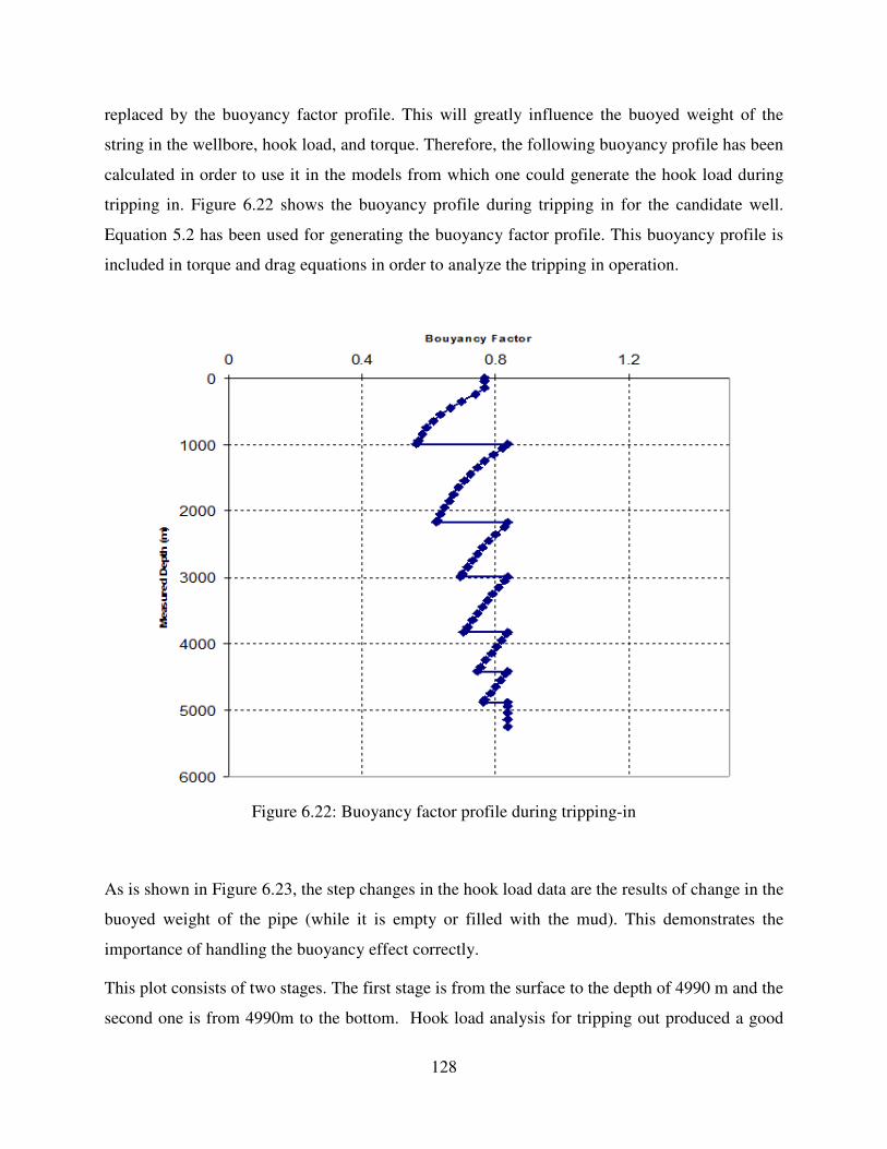
128
replaced by the buoyancy factor profile. This will greatly influence the buoyed weight of the
string in the wellbore, hook load, and torque. Therefore, the following buoyancy profile has been
calculated in order to use it in the models from which one could generate the hook load during
tripping in. Figure 6.22 shows the buoyancy profile during tripping in for the candidate well.
Equation 5.2 has been used for generating the buoyancy factor profile. This buoyancy profile is
included in torque and drag equations in order to analyze the tripping in operation.
Figure 6.22: Buoyancy factor profile during tripping-in
As is shown in Figure 6.23, the step changes in the hook load data are the results of change in the
buoyed weight of the pipe (while it is empty or filled with the mud). This demonstrates the
importance of handling the buoyancy effect correctly.
This plot consists of two stages. The first stage is from the surface to the depth of 4990 m and the
second one is from 4990m to the bottom. Hook load analysis for tripping out produced a good

129
match between the measured data and the models results using a friction coefficient of 0.2. Using
the same friction coefficient for tripping in results in a good match in the first 3000 m. Beyond
3000m, however, a discrepancy between the field data and the models results is observed. This
discrepancy is due to drill string rotation from the surface, which reduces the axial friction.
Figure 6.23: Comparison between the field and models hook load data using a friction coefficient
of 0.2 for tripping in
The back calculation of friction coefficient from the hook load data is shown in Figure 6.24. The
tripping out friction factor is approximately 0.2 everywhere except in the hump interval (Figure
6.19). The tripping in graph shows that the friction factor is close to 0.2 in the upper interval
above 3000 m. For the interval between 3000 m and 3500 m, the friction factor starts to decrease
gradually from 0.2 to 0.1. From the depth 3500 m to the 4890 m, the friction coefficient is almost
0.1.This trend is not observed in the tripping out analysis. This indicates the importance of

130
assessing the axial forces on the pipe whether the pipe is in tension or compression. The tripping
out data shows that the drill string is in tension as it is tripping throughout the wellbore. This
means that in tripping out the pipe is fully contacted on the low side of the wellbore and the
assumption made in the soft string models is valid.
Figure 6.24: Friction coefficient versus the measured depth during tripping in and out
The tripping in pipe conditions is more complex. As it was analyzed, the section from 3200 m is
in compression while the interval above this depth is in tension. Because the condition on the
pipe is changing between tension and compression and the pipe is neither on the low nor high
side, a pseudo-catenary profile forms and the friction is significantly reduced as the contact force
is reduced. This is the case where the normal soft string models could not predict accurately. The
reduction in friction force is noticeable in matching the field data with models using a friction
coefficient of 0.1.
Friction reduction interval
while lowering
Drilling interval

131
Figure 6.25: The tripping in procedure in terms of flow rate and drill string rotation
Figure 6.25 reveals that in the interval between 2990 m to 4000 m, the pipe is running in with the
same axial speed of that in upper intervals. There are 3 pauses in running the pipe which occur at
depths of 1000 m, 2000 m and 3000 m. These depths are the same depths possessing jumps in
hook load data. These jumps occur where the pipe stops to be filled up with the mud.
Another effect that can be addressed is the acceleration of the BHA. Every time one stand is run
in the hole, the string is stopped for connection. Consequently, the BHA has to decelerate before
the full stop. This deceleration creates a peak in the hook load data every time the drill string is
stopped for connection. Figure 6.23 shows that the peaks in the hook load occur every 30m. A
comparison between Figures 6.19 and 6.23 show that the peaks for tripping in are larger than
those for tripping out. This is expected considering the direction in which the deceleration of the
BHA takes place.
Drilling with 150rpm
Drill first stand
gently with 100rpm
Circulation after reaming (rpm=0)
Reaming through tight
spots with ≈50rpm

132
Figure 6.26: Comparison between the field and models torque data using a friction coefficient of
0.2 during tripping in
Figure 6.26 shows the corresponding torque plot during tripping in. The only sections that drill
string is experiencing torque are around 3800 m, 4300 m, and the last 360 m of the well in which
drilling operations has taken place. Here the bit torque is approximately 7.5 KN.m for the drilling
section. The plot shows that the models and field data are quite consistent when using a friction
coefficient of 0.2.
Another factor that has to be considered in the friction analysis is the sheave friction, which is
the result of passing drilling lines through the sheaves. This depends on the number of drilling
lines and block movement direction as well as type of deadline sheave, and whether they are
active or inactive. The effect of this friction in the hook load data were considered for this field
case.

133
6.3 Detection of Drill string Sticking - Analytical Modeling
A well drilled in western Canada is used to illustrate this type of friction analysis. The well
geometry is shown in Figure 6.27. The well depth was 3251 m when the drill string got stuck
during drilling operations. The well profile included a kick off point at 800 m and the heavier
build-up section initiated at 2287 m. The well reached an angle of 30 degree inclination at 2700
m and drilled to a total depth of 3231m with the same inclination of 30 degrees. At this depth,
the drill string was tripped out for the purpose of replacing the measured while drilling (MWD)
tool. The drilling process was continued for a 20m interval after the tripping in procedure. At the
depth of 3251m the drill string got stuck.
Figure 6.27: Well geometry of stuck well
The drill string configuration was not changed from 2200m to 3251 m. The BHA had a length of
290m from the bit. The BHA has a large effect on the value of friction force during tripping in
and out. For example, any interval in the wellbore which has a smaller diameter (due to

134
formation swelling) has a greater friction force against the BHA movement. This behavior is
shown in Figure 6.28.
Friction Coefficient
Bit D
ep
th (
m)
Figure 6.28: Illustration of BHA-tight hole effect on the friction coefficient
As discussed before in Chapter 5, another important factor in friction analysis is the buoyancy
factor, which changes during different drilling operations. In Figure 6.29, the buoyancy factors
of tripping in, drilling and tripping out modes is shown.
During the drilling process, the buoyancy factor is maintained at a constant value until the depth
of 2485 m when the mud weight was increased by 300 kg/m3 to prevent the gas inflow. This
increase led to a decline in the buoyancy factor. The tripping out process exhibits a nearly
constant buoyancy factor since the mud weight is kept constant and the level of mud in the
annulus drops a little. The annulus is filled up periodically through the fill-up lines. The
buoyancy factor during the tripping in process shows a gradual decrease due to the increasing
length of the empty pipe. Since the drill string is filled periodically, some jumps in the buoyancy
factor trend are observed. An increase in the level of drilling fluid inside the drill string leads to
an increase in the buoyancy factor as shown in Figure 6.29.

135
Figure 6.29: Buoyancy factor profile during different operations
The above mentioned increase in mud weight due to gas influx results in a down hole pressure
rise (see Figure 6.30). This increase in the mud weight enhances the differential pressure
between the drill string spots which temporarily and instantaneously stick to the formation and
exerts an additional force on the pipe. Although the increase in mud weight decreases the normal
force on the drill string due to a change in the buoyancy factor, the excess differential pressure
has an effect with a larger magnitude, which in turn increases the frictional force in those spots.
For example, in any pipe sticking problem, the first remedial action is reduction in mud weight in
order to decrease the differential pressure between the drill string and the formation. In most
cases, this reduction may help to release the drill string from the stuck point.

136
Figure 6.30: Mud pressure gradient versus measured depth during drilling operation
Figure 6.31 compares the hook load recorded during tripping in and out. These data are used to
do the friction analysis for this case study. The periodical shifts in hook load values during
tripping in are due to the increased buoyancy factor as the fluid fills the drill string. These jumps
are not observed during tripping out because the buoyancy factor is almost constant due to filling
the annulus using the fill-up lines. A deviation from the hook load trend is observed as the build-
up section begins at the depth of 2287 m due to the increase in friction force in the build-up
section.

137
Figure 6.31: Hook load data versus measured depth during tripping in and out
Figure 6.32 presents the frictional force during the tripping out process. The friction force is
calculated from the difference between the static weight of drill string and the hook load value.
The friction in the curved section is tension dominated showing a rapid increase in the friction
force. As the top of the BHA reaches the build-up section, an increase in the frictional force
occurs at around 2900 m. As the BHA passes through the buildup section, the friction force
declines.

138
Figure 6.32: Friction force versus measured depth during tripping out
The same effect is observed in Figure 6.33 for the overall friction coefficient. The overall friction
coefficient is defined as a single friction coefficient for the entire wellbore. Here, the change in
friction coefficient is the effect of contact surface between the borehole and BHA. This effect
vanishes gradually as the BHA passes through the build-up section.

139
Figure 6.33: Overall friction coefficient versus measured depth during tripping out
The question that arises here is: why should the friction coefficient be calculated for the friction
analysis? To be more precise, is friction coefficient required in addition to the friction force for
this kind of analysis? The answer lies, in that, in some cases the friction force increases due to
the change in well geometry (e.g., increase in dogleg angle). Using a wellbore friction model
helps to isolate the effect of increased friction coefficient from the wellbore geometry effect.
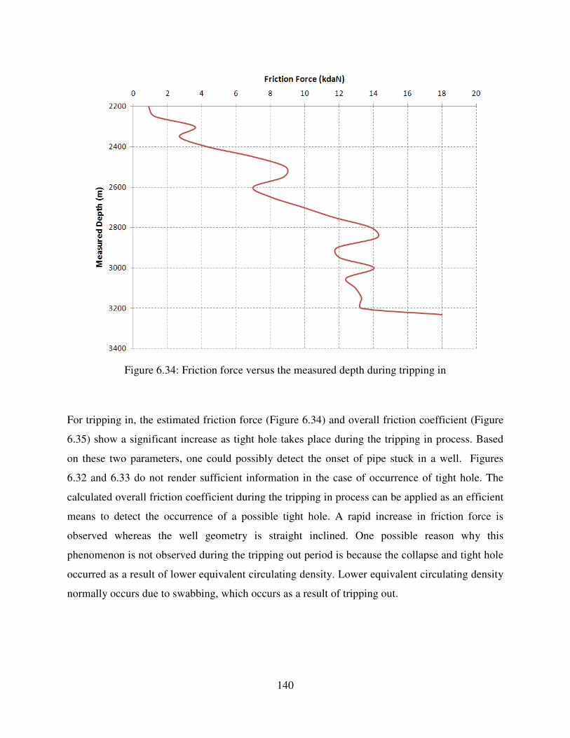
140
Figure 6.34: Friction force versus the measured depth during tripping in
For tripping in, the estimated friction force (Figure 6.34) and overall friction coefficient (Figure
6.35) show a significant increase as tight hole takes place during the tripping in process. Based
on these two parameters, one could possibly detect the onset of pipe stuck in a well. Figures
6.32 and 6.33 do not render sufficient information in the case of occurrence of tight hole. The
calculated overall friction coefficient during the tripping in process can be applied as an efficient
means to detect the occurrence of a possible tight hole. A rapid increase in friction force is
observed whereas the well geometry is straight inclined. One possible reason why this
phenomenon is not observed during the tripping out period is because the collapse and tight hole
occurred as a result of lower equivalent circulating density. Lower equivalent circulating density
normally occurs due to swabbing, which occurs as a result of tripping out.

141
Figure 6.35: Overall friction coefficient versus measured depth during tripping in
6.4 Three Dimensional Well-Finite Element Modeling
In this section, the extended reach well in Section 6.2 is investigated by using the finite element
model. Figure 6.36 shows a comparison between the hook load data for field and finite element
modeling with a friction coefficient of 0.2. In this case study, the model approximately matches
the field data at the bottom hump whereas the top hump is not seen in the model. As it was
previously discussed (Section 6.2), this behavior is attributed to the cuttings accumulation (due
to the upward dragging of the drill string) and the contact surface effect between the BHA and
the wellbore. This case study verifies the analytical model developed in this research. The soft
string analytical model illustrates that the discrepancies between the field and modeling data is
not related to the stiffness of drill string at all. Instead, it may be related to the wellbore
condition, being non-uniform during tripping out.
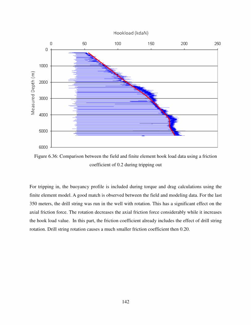
142
Figure 6.36: Comparison between the field and finite element hook load data using a friction
coefficient of 0.2 during tripping out
For tripping in, the buoyancy profile is included during torque and drag calculations using the
finite element model. A good match is observed between the field and modeling data. For the last
350 meters, the drill string was run in the well with rotation. This has a significant effect on the
axial friction force. The rotation decreases the axial friction force considerably while it increases
the hook load value. In this part, the friction coefficient already includes the effect of drill string
rotation. Drill string rotation causes a much smaller friction coefficient then 0.20.

143
Figure 6.37: Comparison between the field and finite element hook load data using friction
coefficient of 0.2 during tripping in
For the torque analysis, the data for the two dimensional well in Section 6.1 was selected. For a
friction coefficient of 0.2, the modeling data lay in the middle of field data points (Figure 6.38).
The field data are for both reaming and back reaming operations and the finite element modeling
data is for the pure rotation without axial movement. For reaming or back reaming operations,
the data trend moves to the right and left, respectively. The latter indicates the effect of combined
motion and decomposing the friction force into rotational and axial components. The fluctuation
of surface torque is considerably more sensitive than that of the hook load. The fluctuations in
surface torque are due to stick slip of some part of the drill string (e.g., stabilizers) during pipe
rotation and bit torques.

144
Figure 6.38: The calculated torque versus measured depth
For the third example, a drilled well in western Canada is selected (Figure 6.39). The well
geometry includes two build-up sections, straight and horizontal sections. The total measured
depth is 3711 m and the length of horizontal departure is almost 1000 m. For drilling the
horizontal well, the hydraulic agitator was added to the drill string to reduce the axial friction
(drag) resulting in sufficient WOB transfer and push pipe was added in the vertical and first
build-up sections. For this well, the hook load data for drilling and tripping out are selected for
torque and drag analysis using the finite element method.

145
Figure 6.39: Geometry of a drilled well including vertical, build-up, straight inclined and
horizontal sections
Figure 6.40 shows the hook load data during drilling. The hook load data usually has high
fluctuations due to variations in weight on bit and drag forces, especially for the horizontal
sections. Using the agitator from the depth of 2800 m causes a smooth transformation of the
applied weight on the bit, which results in obtaining a smoother hook load data trend. A good
match is observed between the field and finite element modeling data. It is worth noting that the
effect of rpm is seen during hook load calculations using the finite element method. The pipe
rotation (i.e., rpm) usually changes during drilling operation from sliding to high surface
rotation.

146
Figure 6.40: Comparison between hook load data of field and finite element modeling data
during drilling
Figure 6.41 compares both analytical and finite element modeling results with tripping out data
for the current well. The tripping out data related to the horizontal section has been selected for
this analysis. The friction coefficient is taken as 0.2 for this analysis. The finite element results
follow the field data trend better than the analytical. It is observed that the analytical result is
over predicting due to full contact assumption (soft string) between drill string and the wellbore.
In finite element modeling, considering the effect of stiffness helps to improve the match
between the modeling and field data.
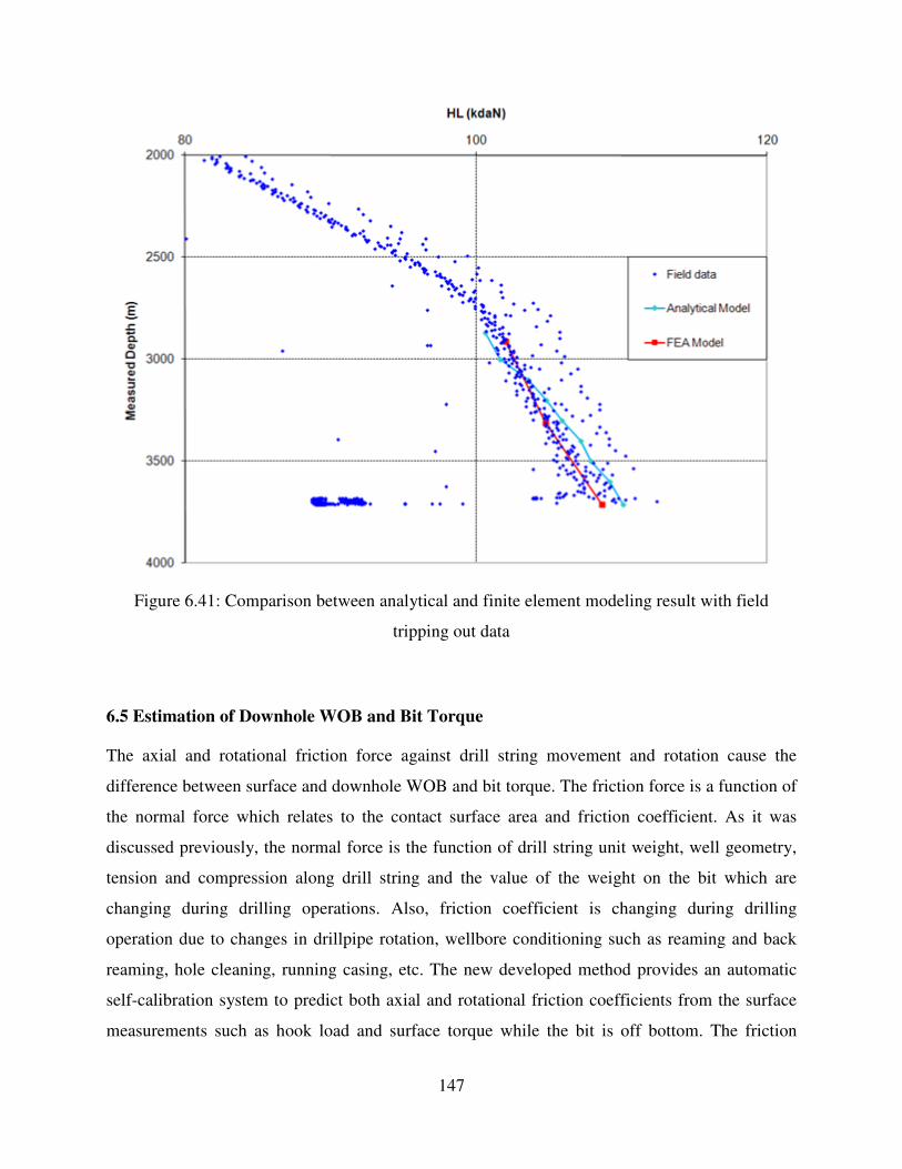
147
Figure 6.41: Comparison between analytical and finite element modeling result with field
tripping out data
6.5 Estimation of Downhole WOB and Bit Torque
The axial and rotational friction force against drill string movement and rotation cause the
difference between surface and downhole WOB and bit torque. The friction force is a function of
the normal force which relates to the contact surface area and friction coefficient. As it was
discussed previously, the normal force is the function of drill string unit weight, well geometry,
tension and compression along drill string and the value of the weight on the bit which are
changing during drilling operations. Also, friction coefficient is changing during drilling
operation due to changes in drillpipe rotation, wellbore conditioning such as reaming and back
reaming, hole cleaning, running casing, etc. The new developed method provides an automatic
self-calibration system to predict both axial and rotational friction coefficients from the surface
measurements such as hook load and surface torque while the bit is off bottom. The friction

148
coefficients are used to calculate the friction forces between drill string and the wellbore while
the bit is on bottom during the drilling operation to estimate downhole weight on the bit and bit
torque. The calculations can involve any torque and drag model using either analytical or finite
element approaches.
This new method can be used for an autodriller system in directional drilling. More particularly,
the autodriller system can estimate downhole weight on the bit and bit torque, from surface hook
load and torque measurements during the drilling operation. Knowing downhole weight on the
bit and bit torque, without running downhole measurement tools, will reduce the cost of drilling
operations significantly.
6.5.1 Background
In the drilling industry, in the absence of downhole measurements, the hook load and surface
torque measurements are used to calculate weight on the bit and the bit torque. Figure 6.42
shows the schematic diagram of a drilling rig. The drilling rig includes a derrick, drill string,
hoisting system, rotating system, circulating system and power system. The derrick supports the
hoisting system and rotating system which is operated by the power system. A drill string
includes a series of drill pipe joints which are connected downwardly from surface into the
borehole. A drilling bit is attached to the end of drill string. The rotating system may include the
rotary table or top drive (not shown) to rotate drill string at the surface to rotate the drilling bit at
the bottom. The hoisting system includes drawworks and a block and tackle system. The
drawworks control the weight on the drilling bit during drilling operations and raise and lower
drill string through the wellbore. The block and tackle system is comprised of crown block,
travelling block and drilling line. If the number of drilling lines in the block and tackle system
increases, the tension in drilling lines is decreased to provide the higher load capacity for the
hoisting system.
The drilling line that is connected to the drawworks from one end, which is called fast line, and
from the other end, which is called the dead line, is connected to the deadline anchor or wheel.
To measure the loads applied on the hook by drill string weight and movement through the

149
wellbore, the hydraulic cell is connected to the deadline to measure the tension in the drilling
line.
Figure 6.42: Schematic illustration of drilling rig that shows the auto driller system is connected
to deadline to estimate downhole weight on the bit
150
For hook load measurement, the measured tension in the deadline should be multiplied by the
number of drilling lines between the sheaves in the block and tackle system. The tension in the
deadline is not a true value due to friction between the drilling line and the sheaves. The true
value is calculated by considering the friction in the block and tackle system. When some weight
of drill string is applied to the drilling bit, a reduction in deadline tension is observed. In the
drilling industry, this reduction is considered as surface weight on the bit which is not usually
equal to downhole weight on the bit. For downhole weight on the bit estimation, the real time
hook load data should be transferred into a new autodriller system for further treatment to obtain
the downhole weight on the bit. Also, the new autodriller can calculate the downhole bit torque
using surface torque measurements. The real time surface torque should be sent to the autodriller
system for downhole bit torque calculation. After calculating downhole weight on the bit and bit
torque, they will be available for users for different purposes such as drilling optimization and
real-time drilling analysis (see Figure 6.42).
Hook load and surface torque measurement values may include the following components
depending on the on and off bottom positions of the drill string.
DWOBFrictionAxialWHL −−=
(6.1)
and
TorqueBitFrictionRotationalTorqueSurface +=
(6.2)
Where W and DWOB represents the static weight of drill string including buoyancy force and
downhole weight on the bit respectively.
To apply weight on the bit, it is required to apply some portion of drill string weight on the bit.
The surface calculated weight on bit is based on the difference between the hook load values
when the drill string is off and on bottom.

151
The surface weight on the bit could be a true value, if the well is vertical and the axial friction
force between drill string and the wellbore is negligible. When the well deviates from a vertical
straight line, the surface and downhole weight on the bit could not be the same due to the axial
friction force between drill string and the wellbore. A similar argument is valid for surface bit
torque calculations. The bit torque is estimated from the difference between surface torque
measurements while the drilling bit is off and on bottom.
The friction force is equal to the friction coefficient multiplied by the normal force which is
applied on the contact surface area of the wellbore. The normal force could be the function of
buoyed unit weight of drill string components, well geometry and the axial (tension and
compression) force along the drill string. For straight sections such as inclined and horizontal
sections, the normal force depends on the buoyed unit weight of drill string components and
compressive load along the drill string. But in curved sections such as build-up and drop-off, the
normal force depends on the buoyed unit weight of the drill string component and the tensile and
compressive loads along the drill string in these sections.
During drilling operations, the friction force acts against drill string axial movement and rotation.
In this case, when applying some weight on the bit, the tension force on drill string elements
located at the curved section will be reduced and friction force will be reduced consequently. If
the tensile load turns into compressive load and exceed the helical buckling, an additional
friction force will be added for increased normal force due to helical buckling.
For downhole weight on bit estimation, the requirements will be the time based drilling
parameters, the static weight of drill string (SWDS), which can be calculated from the vertical
projection of drill string at each measured depth as well as a reliable three dimensional friction
model to calculate friction forces and coefficients along drill string. All these requirements are
programmed and integrated in a real-time controlling system. Downhole weight on bit and bit
torque can be updated as long as surface data are being generated.
6.5.2 Vertical Well
Figure 6.43 (a) illustrates, in a schematic way, a drill string in a vertical wellbore with a hook at
the top. The drill string is hung from the hook which mostly consists of drillpipe and the lower

152
end of the drill string called bottom hole assembly that carries a drilling bit. The borehole is
being drilled and extends downwardly from the surface. In Figure 6.43 (a), the drilling bit is off
bottom and the entire load of drill string applied on the hook. In this condition, the entire drill
string will be in tension. The minimum tension is at the drilling bit and maximum tension will
be at the surface.
(a) (b)
Figure 6.43: Schematic description of drill string moving downwardly in a vertical well while the
bit is off and on bottom, respectively.
Also, there is a negligible contact between drill string and the vertical wellbore during drill string
rotations. This means that the friction force can be neglected. For a drill string element in a
vertical wellbore as shown in Figure 6.43 (a), the tension force balance can be written as follow:

153
WFF bottomtop += (6.3)
To calculate the tension at the hook, drill string is divided to n number of elements and
calculation starts from the drilling bit all the way to the surface. It is noted that in underbalanced
drilling, the buoyancy factor is a dynamic parameter, which will vary along the drill string by
changing the pressure, temperature, drilling cutting rate, gas influx, etc.
Figure 6.43 (b) shows the drill string in the bottom position. Once some weight of drill string is
applied on the drilling bit, some length of drill string compresses beginning from bit to neutral
point. At the neutral point, compression switches to tension for the rest of the drill string to the
surface. Obviously, the hook load will be smaller once the drill string is on bottom; as much as
the weight applied is on drilling bit. In this scenario, the weight on the bit is recorded from the
difference between the hook load values when the drill bit is off and on bottom. The calculated
surface weight on the bit will be the same as what is applied downhole by neglecting the minor
friction in the vertical well. If helical buckling happens in vertical well drilling, it creates some
additional friction force that should considered in vertical drilling for downhole weight on bit
estimation. The force balance at each element can be written as follow:
[ ] DWOBorFrictionWFF helicalbottomtop −−+= 0 (6.4)
When the bit is off bottom, the surface torque value is negligible due to minor contact between
drill string and the vertical wellbore. Once the bit goes on bottom for drilling and applies weight
on bit, an increase in value of surface torque can be observed due to bit torque. To calculate bit
torque from surface measurements, the difference between surface torques while bit is off and on
bottom should be calculated.

154
6.5.3 Extended Reach Well
For extended reach well drilling, Figure 6.44 (a) shows a drill string in a wellbore which consist
of vertical, build-up and straight inclined sections. In the build-up and straight inclined sections,
there is contact between drill string and the wellbore which results in a friction force against the
pipe movement. The nature of friction in these two sections is different. In this scenario, the bit
is off bottom and the entire drill string is in tension. When the axial friction force calculations
start from the drilling bit and upward, in the straight inclined section the tension will not have
any contribution in axial friction force. But as the build-up sections begin, the tension at this
point will have a great contribution in the friction force. It means, for a drill string element in the
straight incline, the friction force only depends on the weight of element which applies normally
on the contact area. But in the build-up section, the friction force mostly depends on the tension
at the bottom of the element and also the normal weight of the drill string element.
(a) (b)
Figure 6.44: Schematic of drill string moving downwardly in a well with the geometry of
vertical, build-up and the straight inclined sections

155
The following is the general force balance for each element along drill string for off bottom
position.
[ ]helicaltensionweightbottomtop FrictionororFrictionFrictionWFF 0−−+= (6.5)
In this equation, the axial friction force term related to tension will be zero if the element is in the
straight section. Also, if the pipe element is placed in the vertical section both terms related to
friction will vanish.
In Figure 6.44 (b), some weight of drill string applies to the drill bit which means reduction in
tension along the drill string. The reduction in tension has considerable effect on the axial
friction force in the build-up section but not straight inclined. If applying the weight on the bit
causes the drill string to be in compression in the curved section, the axial friction force for that
part will not be a function of the tension anymore and it should be treated the same as straight
inclined elements. The Equation 6.6 represents the force balance when applying weight on the
bit.
[ ] DWOBFrictionororFrictionFrictionWFF helicaltensionweightbottomtopDWOB
−−−+= 0 (6.6)
In Equation 6.6, the friction force in the curved section is affected by downhole weight on the bit
which is subscripted by DWOB. It should be mentioned that the axial friction force changes in
the curved section and will change the overall friction and surface hook load value consequently.
If the downhole weight on the bit helically buckled the pipe element, then the additional friction
should be considered, as discussed in Chapter 5.
The same argument is valid for the surface torque measurements. The rotational friction force
between drill string and wellbore depends on the normal weight of drill string element and
tension along the drill string. Applying weight on the bit reduces the tension along the drill

156
string, which affects the value of rotational friction force in the curved section. Equation 6.7
shows the torque for an element in drill string while the bit is off bottom and there is no weight
on the bit.
[ ]0orTorqueTorqueTorqueTorque tensionweightbottomtop ++= (6.7)
To calculate the surface torque, the drill string is divided into many elements; and calculation
starts from the bottom to the surface. Once the element is in a straight inclined section, the torque
will be the function of the element weight only. When the element is in the curved section and
the drill string is in tension, the torque will depend mostly on tension and less on weight. For
surface torque, when the drill string goes on bottom, the tension along drill string will change.
The latter affects the value of rotational friction force in the curved section as well. Also, the
value of torque on the bit will be added as shown in Equation 6.8. The rotational friction force in
the straight inclined section will not change.
[ ]helicaltensionweightbottomtop TorqueorTorqueTorqueTorqueTorqueDWOBDWOB
0++= (6.8)
6.5.4 Horizontal Well
Figure 6.45 (a) shows a horizontal well which includes vertical, build-up and horizontal sections.
The drill string is off bottom and pushing toward the bottom. The axial friction force is acting
against the drill string movement tendency. To push the pipe in the horizontal section, it is
necessary to have some heavy drillpipes in the vertical and build-up sections to provide sufficient
drive to push the drill string in the horizontal section. The axial friction force in the horizontal
section is a function of the weight of drill string, which is normally applied on the wellbore
contact area as well as additional friction force due to helical buckling. When the drill bit is off
bottom and the drill string is pushing toward the bottom, some part of heavy drillpipe will be in
compression due to axial friction force in the horizontal section. In this scenario the axial
friction force in the curved section, which is in compression, is a function of the weight of drill

157
string element and compressive load if it exceeds the helical buckling load. Above the neutral
point, the drill string will be in tension and axial friction force will depend on the normal force
and tension force for each element. Equation 6.5 can be applied to horizontal well drilling for
hook load calculation when the drill bit is off bottom and moving toward the bottom.
When some weight is applied on the bit (as shown in Figure 6.45 (b)), more of the drill string
becomes compressed. In this case, usually most of the axial friction force in the build-up section
will no longer depend on the tension. Equation 6.6 can be applied for the hook load calculations
when the drill bit is on bottom and some weight is applied to the bit.
(a) (b)
Figure 6.45: The drill string along a horizontal well which is pushing toward the bottom
In Figure 6.45 (a), once the drill string is off bottom, there is no bit torque. The rotational friction
force is related to build-up and horizontal sections. In the horizontal section, the rotational
158
friction force is the function of normal force, which is applied by the weight of drill string
element as well as compressive load if the axial load exceeds the helical buckling load. In the
build-up section while the drill string element is in compression, the rotational friction force is
the function of weight or maybe the compressive load. However, if drill string is in tension, the
rotational friction force is the function of tension and weight. Once the drill bit goes on bottom
(see Figure 6.45 (b)), applying weight on drill bit causes some reduction in tension along the drill
string, which affects the value of rotational friction force in the build-up section. During the
drilling operation, there are some variations in bit torque and rotational friction force in the
curved section. These should be estimated from surface torque measurements using the new
method presented in this work.
6.5.5 Description of System
Figure 6.46 is a general flowchart showing the steps how to estimate downhole weight on the bit
from surface measurements. The first step is determining the static weight of drill string, SWDS.
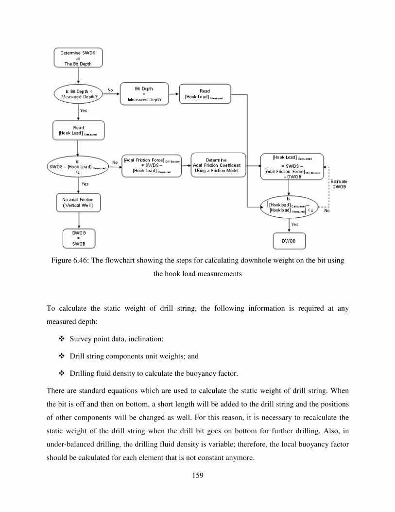
159
Figure 6.46: The flowchart showing the steps for calculating downhole weight on the bit using
the hook load measurements
To calculate the static weight of drill string, the following information is required at any
measured depth:
Survey point data, inclination;
Drill string components unit weights; and
Drilling fluid density to calculate the buoyancy factor.
There are standard equations which are used to calculate the static weight of drill string. When
the bit is off and then on bottom, a short length will be added to the drill string and the positions
of other components will be changed as well. For this reason, it is necessary to recalculate the
static weight of the drill string when the drill bit goes on bottom for further drilling. Also, in
under-balanced drilling, the drilling fluid density is variable; therefore, the local buoyancy factor
should be calculated for each element that is not constant anymore.

160
The second step is determining if the bit is off or on bottom. During drilling operations, the mud
logging unit records all necessary field data. The measured depth and bit depth data will be used
to know when the bit is off and on bottom and also if bit is moving upward or downward. The
measured depth corresponds to final drilled depth. When the bit is off bottom and the drill string
is moving downward, the measured hook load should be compared with the static weight of drill
string. If the difference between values is negligible, it means there is no axial friction force and
the well geometry is vertical. When the bit goes on bottom, some weight of drill string applies to
the bit and a reduction in the hook load will be observed. The reduction in the hook load is taken
as downhole weight on bit. Therefore, the downhole weight on bit can be calculated directly
from the surface hook load measurements for a vertical well when the drill bit is off and on
bottom.
If the difference between measured hook load and the static weight of drill string is not
negligible, the difference between these two values provides the axial friction force between the
drill string and the wellbore. It is critical to select the best measured hook load value while the
bit is off bottom because the axial friction coefficient is estimated based on it. The estimated
axial friction coefficient will be used for estimating the downhole weight on the bit when the
well is deviated and there is considerable axial friction force between drill string and the
wellbore. Therefore the following conditions are considered to select the best measured hook
load value while the bit is off bottom:
The hook load is chosen when the bit is moving downwardly very close to bottom hole.
In this situation, the drill string movement is very slow similar to the on-bottom situations
where the drill bit is penetrating a formation.
The drill string rotation speed and flow rate are the same as planned ones while the bit
goes on bottom for further penetration. The effect of pipe rotation is included in axial
friction coefficient.
By knowing the axial friction force and having a reliable friction model, the axial friction
coefficient (which includes the drill string rotation effect) will be estimated. This axial friction
coefficient will be used for the estimation of downhole weight on the bit when the bit goes on
bottom for further drilling.

161
When the bit depth and the measured depth are equal it means the bit is on bottom. In this
situation, the measured hook load is known and the hook load could be calculated as well. To
calculate the hook load, the static weight of drill string, axial friction force and downhole weight
on the bit should be known. As discussed, the static weight of drill string is obtained directly
from the aforementioned standard equations. The downhole weight on the bit is estimated and
the axial friction force will be calculated based on estimated downhole weight on the bit. Here, to
obtain the best value for downhole weight on the bit, some value should be estimated close to
surface weight on the bit and applied to the friction model to see its effect on the value of axial
friction force. If the difference between measured and calculated hook load is negligible then the
value is taken as true, otherwise another value is chosen and the calculation is repeated.. This
loop will be continued until the difference between the calculated and measured hook load values
become negligible.
Figure 6.47 is a general flowchart showing the steps to estimate the bit torque when rotating
from the surface. The procedure is similar to downhole weight on the bit. The estimated
downhole weight on the bit in the previous section is used for downhole bit torque calculation. In
the first step, the bit depth should be compared with measured depth to see if the drilling bit is on
bottom or off bottom. When the drill bit is off bottom and the value of the measured surface
torque is negligible, it means the drilling well is vertical and there is negligible rotational friction
force. When the drill bit goes on bottom for further drilling, the measured surface torque almost
corresponds to downhole bit torque. If the measured surface torque is not negligible while the bit
is off bottom, it means the well is not vertical and there is rotational friction force against the
drill string rotation. As discussed before, the best selected data for friction coefficient estimation
is when the bit is off bottom and is moving downwardly close to the bottom with the same pipe
rotation as planned for drilling. From the rotational friction force while bit is off bottom and
using a reliable friction model, the rotational friction coefficient could be estimated for the next
steps.

162
Figure 6.47: The flowchart showing the steps for the calculation of downhole bit torque by using
the surface torque measurements
When the bit goes on bottom for further drilling, the measured surface torque can be read. The
downhole weight on bit will affect the rotational friction force due to changes in tension along
the drill string. Using the downhole weight on bit and the rotational friction coefficient in a
reliable friction model yields the rotational friction force during drilling operation which changes
with the changes in downhole weight on the bit. The final step is calculating the downhole bit
torque due to surface rotation by subtracting the rotational friction force from surface torque
measurements.
6.5.6 Example Application
To show the application of this method, a newly developed analytical friction model is used to
see how the downhole weight on bit and bit torque can be calculated during drilling operations.
When drill string specification, survey data and friction coefficient are specified, the calculation
begins at the bottom of the drill string and continues stepwise upwardly. Each drill string element

163
contributes small load on hook load and surface torque. The force and torque balance on drill
string element when the bit is off bottom can be written as follow:
( )helicalbottombottom
bottomtop
bottomtop
bottomtop
bottomtop
top
FrictioneForF
orLworLwF
−×+
−
−∆×−
−
−∆=
− θµ
αα
αααβµ
αα
αααβ
coscossin
sinsincos
(6.9)
For the torque at each element:
( )θµαα
αααβµ ×××+
−
−×∆××+= bottom
bottomtop
bottomtop
bottomtop FrororLwrTT 0coscos
sin (6.10)
and when the bit is on bottom, there is some weight on the bit which affects tension along drill
string:
[ ]( )DWOBhelicalbottombottom
bottomtop
bottomtop
bottomtop
bottomtop
top
FrictioneDWOBForDWOBF
orLworLwF
−×−−+
−
−∆×−
−
−∆=
− θµ
αα
αααβµ
αα
αααβ
coscossin
sinsincos
(6.11)
For the torque at each element:
[ ]( )θµ
αα
αααβµ
×−××
+
−
−∆×+=
DWOBFror
orLwTT
bottom
bottomtop
bottomtop
bottomtopDWOB
0
coscossin
(6.12)
In Equations 6.9 and 6.11, the terms in order for a drill string element correspond to static
weight, the axial friction force caused by the weight and axial friction force caused by the

164
tension and compression at the bottom. In the equations, if the inclination at the top and bottom
of an element is equal, the element is considered as straight and the first term in each bracket will
be used, otherwise it will be considered as a curved element and the second term will be used.
When weight is applied on the bit, the effect of downhole weight on the bit can be integrated as
shown in Equation 6.11, which reduces the tension along the drill string and reduces the axial
friction force in the curved section. If any curved element is in compression, the effect of tension
on the axial friction force will be eliminated. For friction term related to helical buckling, if the
compressive load exceeds the helical limit, the equations presented in Chapter 5 should be used.
Furthermore, for bit torque calculation, it is necessary to calculate the rotational friction force
from drill bit to the surface. Equation 6.10 is used to calculate the rotational friction force for
each element while the drill bit is off bottom. The first term in each bracket is used when the
elements are located in straight sections and the second term is used for the elements which are
placed in curved sections. It should be noted that when the element is compressed in the curved
section, the rotational friction force will only be a function of the weight of the element. When
the drill string goes on bottom, the downhole weight on the bit causes the reduction in tension
along drill string, which significantly reduces the rotational friction force.
A drilled well has been selected as shown in Figure 6.39 to illustrate how an autodriller can
estimate the downhole weight on the bit and bit torque. The well geometry includes two build-up
sections, straight and horizontal sections.
When the drill bit is at the depth 2700 m, the entire drill string was is in tension. Applying 11
kdaN weight on the bit causes some portion of the drill string starting at the bit to compress and
reduce the tensile force for the rest, as shown in Figure 6.48.

165
Figure 6.48: Comparison between tension and compression along drill string when 11kdan
weight is applied on the bit
Figure 6.49 illustrates that the reduction in tension along the drill string has an effect on the
friction force (2.15 kdaN). In the example, the downhole weight on the bit merely affects the
friction force in the build-up sections. As discussed before, the weight on the bit reduces the
friction force in the curved sections, which affect the axial and rotational friction force.

166
Figure 6.49 shows reduction in axial friction force along drill string when 11 kdaN weight is
applied on the bit.
The sample calculation for this example is as follow:
When the bit is at the depth 2695.6 m, almost 0.4 m off bottom and moving downwardly, the
axial friction coefficient including the pipe rotation effect, is estimated as follow:
[ ] kNLoadHookDepthMeasuredDepthBit
mDepthMeasured
mDepthBit
kNStringDrillofWeightStatic
MesauredOff 2.810
02.2696
6.2694
4.874
=→≤
=
=
=
[ ] ( )includedrotationpipekNForceFrictionAxial axial
ModelFrictiongU
BottomOff095.04.642.8104.874
sin= →=−= µ

167
The axial friction coefficient including the pipe rotation effect is used when the drill string goes
on bottom for drilling. The axial friction coefficient can be updated for each wiper trip (or in
some cases connections) periodically and used for upcoming sections. The estimated axial
friction coefficient is used in a friction model to calculate the hook load.
[ ]kNSWOB
kNLoadHookDepthMeasuredDepthBit
mDepthMeasured
mDepthBit
MesauredOn
94
760
02.2696
02.2696
=
=→=
=
=
The different values for downhole weight on the bit should be estimated until the difference
between the measured and calculated hook loads becomes negligible. When the difference is
acceptable, the final estimated value for downhole weight on the bit is chosen.
kNDWOB, [ ] kNHookload Calculated , [ ] [ ] kNHookloadHookloadMeasuredCalculated 00.1≤−
SWOB=94 739.5 20.50
90 742.9 17.10
85 746.9 13.10
80 751 9.00
75 745 5.00
DWOB = 70 759 1.00
Figure 6.50 compares surface and downhole weight on the bit values for a one meter drilled
interval using the present invention method.

168
Figure 6.50 Comparison between surface and downhole weight on the bit for 1m drilled interval
For surface torque measurement, the increment in surface torque when the drill bit goes on
bottom for drilling is considered bit torque. The reduction in tension has a considerable impact
on the rotational friction force, which should be counted for bit torque calculations. In this field
example, when the bit is off bottom and moving downwardly with the same rpm as planned for
drilling, the measured surface torque is as follow:
[ ] mkNTorqueSurfaceDepthMeasuredDepthBit
mDepthMeasured
mDepthBit
Measured.5.13
09.2696
6.2695
=→≤
=
=

169
The measured surface torque is equal to rotational friction force. By using a reliable friction
model, the rotational friction coefficient can be estimated:
[ ] 245.0.5.13sin
= →= Rotational
ModelFrictiongU
bottomoffmkNForceFrictionRotational µ
When the drill bit is on bottom and some weight is applied to the drill bit, the surface torque
measurement increases due to interaction between drill bit and rock surface. The difference
between surface torque measurements for off and on bottom drilling positions, considered as
surface bit torque, are shown as follow:
[ ] mkNTorqueBitSurfacemkNTorqueSurfaceMeasured
bottomon .36.15.1386.14.86.14 =−=→=
When some weight is applied to the bit, the tension along the drill string will be reduced. The
rotational friction force is reduced as well, which should be considered for bit torque
measurements.
[ ] mkNForceFrictionRotationalkNDWOB
bottomon.34.12
120 →
=
The downhole torque at the bit can be estimated as follow:
[ ] [ ]mkN
ForceFrictionRotationalTorqueSurfaceTorqueBitDownholebottomonMeasured
bottomon
.52.234.1286.14 =−=
−=

170
Figure 6.51 compares the surface and downhole bit torque for one meter interval by considering
the effect of downhole weight on the bit on rotational friction force.
Figure 6.51: shows the surface and downhole bit torque for 1m drilled interval
6.5.7 Field Application
Figure 6.52 shows the well geometry of a field example, which verifies the application of the
current method. A 350 m horizontal drilled interval was selected to estimate the downhole
weight on the bit from the hook load measurements. As discussed previously, the friction
coefficient should be estimated and updated during the drilling operation.

171
Figure 6.52: Geometry of a short bend horizontal well including vertical, build-up and horizontal
sections
During drilling this 350 m horizontal interval, the drilling conditions are changed continuously.
For example, the surface rotation changed from zero, sliding mode, to 30 rpm. As previously
discussed, the mud rheology, cutting bed formation, and drill string positions affect the friction
coefficients. Figure 6.53 illustrates the plot of friction coefficient including drill string rotation
effect versus measured depth for this 350 m drilled interval used for the downhole weight on the
bit estimation.

172
Figure 6.53: Plot of friction coefficient versus measured depth during drilling operation for the
interval between 3070 m to 3420 m
Figure 6.54 compares the surface and downhole weight on bit estimated using the new designed
autodriller system. It can be concluded that the effective weight on the bit is almost half of what
the drilling crew thought. An autodriller system may help the drilling crew to apply the desired
optimum weight on the bit to improve the drilling rate of penetration without concerns of drill
string buckling and premature bit wear. Additionally, for drilling optimization that uses the offset
drilling data, it is necessary to use the correct weight on the bit data as an input to this system.
Using raw weight on the bit data, especially horizontal data, can show higher rock strength
which would directly affect the drilling optimization output results.
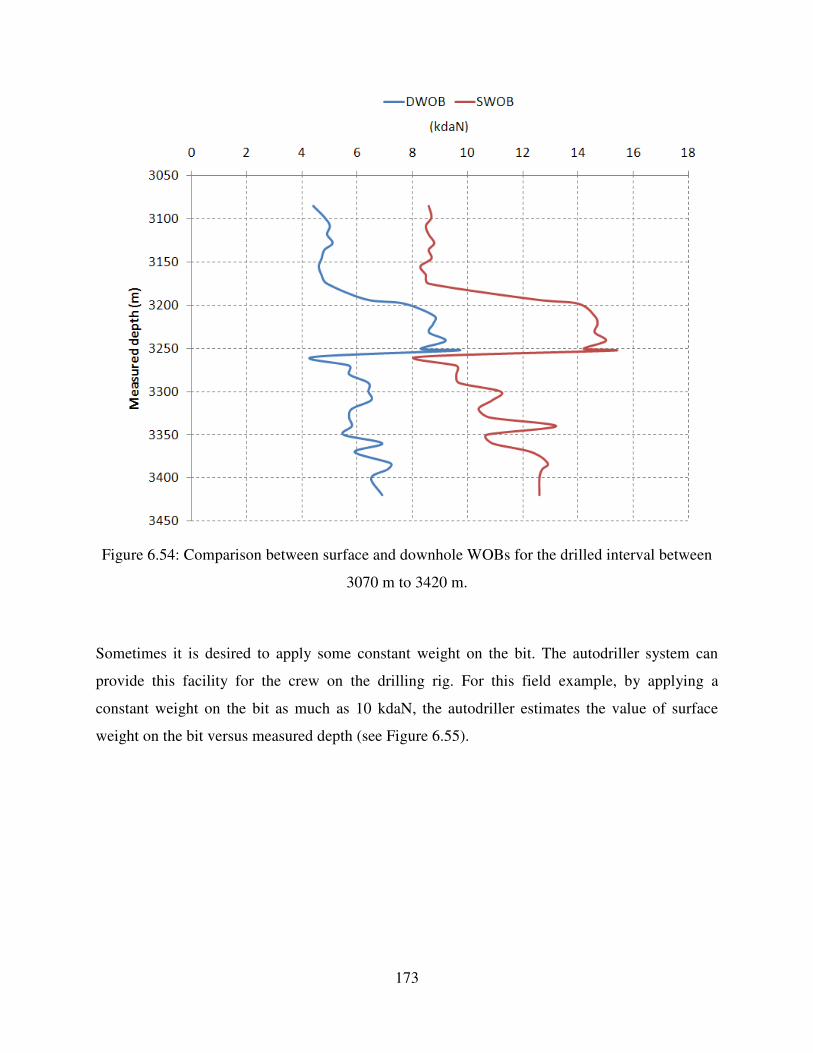
173
Figure 6.54: Comparison between surface and downhole WOBs for the drilled interval between
3070 m to 3420 m.
Sometimes it is desired to apply some constant weight on the bit. The autodriller system can
provide this facility for the crew on the drilling rig. For this field example, by applying a
constant weight on the bit as much as 10 kdaN, the autodriller estimates the value of surface
weight on the bit versus measured depth (see Figure 6.55).

174
Figure 6.55: Plot of surface WOB values versus measured depth during drilling operation when
keeping 10 kdaN downhole weight on the bit
This autodriller system can be also used for sliding mode drilling which is used to orient tool
face in directional or horizontal drilling. The drilling bit is rotated by the mud motor instead of
rotating the drill string from surface. The mud motor is powered by the fluid differential
pressure. There is a certain relationship between differential pressure and downhole weight on
the bit, which can be found by using the present system. Here, the “K” value is used to represent
the ratio of estimated downhole weight on the bit to differential pressure which can be found
during the drilling rotating time. When sliding begins, a new downhole weight on the bit can be
predicted with the product of K and differential pressure. As an example, the average value for
“K” is estimated during rotating time as kPa
kN67.0 for a drilled interval. The differential
pressure was multiplied by “K” value to estimate the downhole weight on the bit as shown in
Figure 6.56
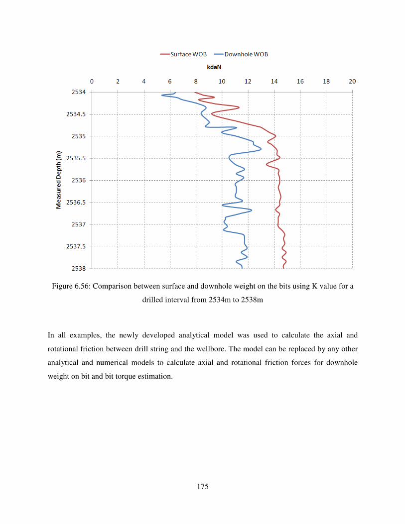
175
Figure 6.56: Comparison between surface and downhole weight on the bits using K value for a
drilled interval from 2534m to 2538m
In all examples, the newly developed analytical model was used to calculate the axial and
rotational friction between drill string and the wellbore. The model can be replaced by any other
analytical and numerical models to calculate axial and rotational friction forces for downhole
weight on bit and bit torque estimation.

176
CHAPTER SEVEN: CONCLUSIONS AND RECOMMENDATIONS
The two following main contributions are made as part of this thesis:
The new models for torque and drag calculations were developed using both analytical
and finite element approaches. The models are simple and practical and can be used in
real time analysis. Also, all possible contributions related to torque and drag analysis
were studied and the ways on how to integrate them in the modeling were proposed.
A new method was introduced for the downhole weight on bit and bit torque estimation
using torque and drag modeling. The new method uses the surface measurements such as
hook load and surface torque as well as information related to drill string, well geometry
and drilling fluid system.
The major conclusions that can be drawn from this thesis are summarized as follows:
The new analytical model consists of two sets of equations for straight and curved
sections. This model is three dimensional and it can consider the effects of build-up or
drop-off bend combined with the side bend simultaneously.
The new analytical model is applicable for all operations such as drilling and tripping
in/out, combined motions (such as reaming and back reaming operations where the pipe
is rotated and pulled or lowered at the same time).
The hydrodynamic viscous force is considered during different operations. A procedure
with a set of equations was presented for the drilling fluid model (Bingham-plastic).
Ignoring this effect results in a little higher friction coefficient.
A simple equation was presented for considering the contact surface effect. It can be
multiplied with the friction coefficient and used in the modeling.
The torque and drag analysis inside a wellbore should be carefully performed. Correct
assessment of buoyancy and the effect of the well path were shown to be critical for
precisely estimating the friction coefficient.
In wellbore friction analysis, the buoyancy effect should be treated precisely. In tripping
in when the drill string is partially filled with drilling fluid, ignoring this effect could
result in an erroneous estimation of the overall friction coefficient.

177
The friction force analysis demonstrated the difference between rotating the string and
not rotating the string. Rotation not only changes the direction of friction force, it also
results in a change of axial tension that may change the total friction. Proper calibration is
required to determine the true value for the friction coefficient including the drill string
rotation effect.
Wellbore friction is a critical parameter not only to drill oil wells, but also during casing
running and completion operations. Running the casing in long reach wells is usually one
of the most critical operations.
In real time torque and drag analysis, using the friction coefficient instead of friction
force provides the possibility to exclude the effect of well geometry on the friction force.
A finite element model was developed for the torque and drag analysis. Using the
equation of motion for development of the model, the effects of drill string stiffness and
vibration were considered.
The validity of finite element model was verified analyzing examples with different
complicity. The values of displacement from the finite element model matched the field
data. It was shown that the result pertinent to the calculation of hook load and surface
torque is convincible.
The finite element modeling rendered a smaller friction coefficient relative to the
analytical one due to the consideration of the partial contacts between the drill string and
the wellbore. In the analytical modeling based on the soft string assumption, the drill
string has full contact with the wellbore.
The new method for the estimation of downhole weight on the bit was presented. The
method comprised the steps of: a) determining the static weight of drill string; b)
determining the axial friction coefficient including pipe rotation effect; c) determining the
effect of downhole weight on the bit on value of axial friction force during drilling; d)
determining downhole weight on the bit using the axial friction coefficient and surface
hook load measurements.
The new method for estimating downhole bit torque was presented. The method
comprised the steps of: a) determining the rotational friction force while the drill bit is off
bottom; b) determining the rotational friction coefficient including axial pipe movement
effect from surface torque measurements while bit is off bottom; c) determining the effect
178
of downhole weight on bit on the rotational friction force during drilling; d) determining
downhole bit torque using the rotational friction coefficient and downhole weight on the
bit.
The new method can be used in an autodriller as a "black box" system for the user to
adjust the hook load and surface torque so that the desired downhole weight on the bit
and bit torque can be obtained.
Using the proposed new method, no downhole weight on the bit measurements is
required, which can help to reduce the drilling cost.
Using the new method, the axial friction coefficient including the drill string rotation
effect can be estimated using the friction model from the best surface measured hook
load. The best measured hook load is while the bit is very close to bottom moving
downwardly. In this situation, the drill string rotation will be the same as the planned one
for drilling a new section.
In the new method for the downhole weight on the bit and bit torque estimation, the
effect of variations in tension and compression on the friction force as well as hook load
and surface torque has been considered. For example, when applying weight on the bit,
the axial friction in the curved section will be reduced. This reduction cannot be
recognized at the surface from surface weight on the bit.
For the estimation of downhole weight and torque on the bit, when the weight is applied
on the bit, if a drill string element in the curved section is in compression, the rotational
friction force is only a function of the weight and not the tension anymore. This means
the effect of tension on the rotational friction force vanishes and considerable reduction
in rotational friction force occurs. If the compressive load exceeds the helical buckling
load, additional friction should be estimated for this effect.

179
References
Aadnoy, S.A., “Friction Analysis for Long-Reach Wells”, SPE/IADC 39391 presented at
SPE/IADC Drilling Conference, Dallas, Texas, March 1998.
Aadnoy, B. S., “Mechanics of Drilling”, Shaker Verlag Aachen, Germany, 2006.
Aadnoy, B.S. and Andersen, K., “Design of Oil Wells Using Analytical Friction Models”,
Journal of Petroleum Science and Engineering, September 2001.
Aadnoy, B. S. and Djurhuus, J., “Theory and Application of a New Generalized Model for
Torque and Drag”, SPE/IADC 114684 presented at the SPE/IADC Asia Pacific Drilling
Technology Conference and Exhibition, Jakarta, Indonesia, August 2008.
Aadnoy, B.S., Fabiri, V.T. and Djurhuus, J., “Construction of Ultra-long Wells Using a Catenary
Well Profile”, SPE/IADC 98890 presented at the SPE/IADC Drilling Conference, Miami,
February, 2006.
Aadnoy, B.S., Fazaelizadeh, M. and Hareland, G., “A 3-Dimentional Analytical Model for
Wellbore Friction”, Journal of Canadian Petroleum Technology, Volume 49, Issue 10, Page
25-36, October 2010.
Aadnoy B.S and Kaarstad, E.; “Theory and Application of Buoyancy in Wells”, IADC/SPE
101795 presented at IADC/SPE Asia Pacific Drilling Tech. Conf. and Exhibition, Bangkok,
Thailand, November 2006.
Aadnoy, B. S., Larsen, K. and Berg, P.C., “Analysis of Stuck-Pipe in Deviated Boreholes”, SPE
56628 presented at the SPE Annual Technical Conf. and Exhibition, Houston, Texas, October
1999.
Aarrestad, T.V., “Effect of Steerable BHA on Drag and Torque in Wells”, SPE 20929 presented
at Europec 90, The Hague, Netherlands, October 1990.
Aarrestad, T.V. and Blikra, H., “Torque and Drag- Two Factors in Extended-Reach Drilling”,
Journal of Petroleum Technology, September 1994.

180
Anston, M.S., Hearn, P.J. and McGhee, G., “Techniques for Solving Torque and Drag Problems
in Today’s Drilling Environment”, SPE 48939 presented at the Annual Technical Conference
and Exhibition, New Orleans, Louisiana, September 1998.
Barakat, E. R., “An Experimental Study and Modeling of the Effect of Hydraulic Vibrations on
Axial Force Transfer in Horizontal Wellbores”, Drilling Research Project for TUDRP
Advisory Board Meeting, Tulsa, Oklahoma, November 14-15, 2005.
Besaisow, A. A., Jan, Y. M. and Schuh, F. J., “Development of a Surface Drill string Vibration
Measurement System” SPE 14327, SPE Annual Technical Conference and Exhibition, Las
Vegas, Nevada, September, 1985.
Bourgoyne, A. T. Jr., Millheim, K. K., Chenvert, M. E. and Young, F. S. Jr., “Applied Drilling
Engineering”, SPE, Richardson, Texas, United States of America,1986.
Brett, J. F., Beckett, A. D., Holt, C. A. and Smith, D.L., “Uses and Limitations of Drill string
Tension and Torque Models for Monitoring Hole Conditions”, SPE Drilling Engineering,
September 1989.
Bueno, R.C.S. and Morooka, C.K., “Analysis Method for Contact Forces between Drill string-
Well-Riser”, Society of petroleum Engineers, SPE 28723, International Petroleum Conference
and Exhibition, Veracruz, Mexico, October 1994.
Burkhardt, J. E., “Wellbore Pressure Surges Produced by Pipe Movement. Society of Petroleum
Engineers”, SPE 1546, Annual Conference in Denver, October 2-5, 1960.
Dangerfield, J. W., “Analysis Improves Accuracy of Weight Indicator Readings”, Oil and Gas
Journal, August 10, 1987.
Dareibg, D.W and Livesay, B. J., “Longitudinal and Angular Drill string Vibration with
Damping”, Journal of Engineering for Industry, Pages 1-9, 1968.
Discovery Channel Online, “Drilling in Different Direction”, Retrieved from:
http://licencetodrill.ca/Articles/directional_drilling.aspx, October 01, 2011.
Dukkipati, R. V., “Matlab for Mechanical Engineers”, Tunbridge Wells: New Age Science,
United States of America, 2009.

181
Dykstra, M. W., “Nonlinear Drill string Dynamics”, Ph.D. Dissertation, The University of Tulsa,
United States of America, 1996.
Eek-Olsen, J., Drevdal, K.E., Samuell, J. and Reynolds, J., “Designing Directional Drilling to
Increase Total Recovery and Production Rates” SPE/IADC Drilling Conference, 27461,
Dallas, Texas, February 15 – 18, 1994.
Falconer, I. G., Belaskie, J. P. and Variava, F., “Applications of a Real Time Wellbore Friction
Analysis”, SPE/IADC 18649 presented at the SPE/IADC Drilling Conference, New Orleans,
Louisiana, February-March 1989.
Fazaelizadeh, M., Hareland, G. and Aadnoy, B. S., “Application of New 3-D Analytical Model
for Directional Wellbore Friction”, Journal of Modern Applied Science, February 2010.
M. Fazaelizadeh, G. Hareland, Z. Wu and M. Tahmeen; “Wellbore Friction Analysis to Detect
Onset of Drill string Sticking during Extended Reach well Drilling: Case Study”, Brazil
Offshore Conference and Exhibition, Macae, Brazil, 14-17 June 2011.
Halliburton Online, “Measurement While Drilling” Retrieved October 07, 2011, from:
http://www.halliburton.com/ps/default.aspx?navid=1754&pageid=129&prodgrpid=MSE%3a%3
a1045856811401511.
He, X., Halsey, G.W., and Kyllingstad, A., “Interactions between Torque and Helical Buckling
in Drilling”, Annual Technical Conference and Exhibition, Dallas, Texas, October 1995.
Ho, H.S., ”An Improved Modeling Program for Computing the Torque and Drag in Directional
and Deep Wells”, SPE 18047 presented at the Annual Technical Conference and Exhibition,
Houston, Texas, October 1988.
Lesage, M., Falconer, I. G. and Wick, C. J., “Evaluating Drilling Practice in Deviated Wells with
Torque and Weight Data” SPE Journal of Drilling Engineering, SPE 16114, September 1988.
Lesso, W. G., Mullens, E. and Daudey, J., “Developing a Platform Strategy and Predicting
Torque Losses for Modeled Directional Wells in the Amauligak Field of the Beaufort Sea,
Canada”, SPE 19550, Annual Technical Conference and Exhibition, San Antonio, Texas,
October 1989.

182
Li, Z., Liu, X., Zhou, D. and Zhang, S., “A Steady Tension-Torque Model for Drill string in
Horizontal Wells”, SPE 26295 presented at USMS Conference, May 1993.
Liu, X. and Samuel, R., “Catenary Well Profile for Extended and Ultra-Extended Reach Wells”,
SPE 124313 presented at the Annual Technical Conference and Exhibition, New Orleans,
October 2009.
Luke, G. R. and Juvkam-Wold, H.C., “Determination of True Hook Load and Line Tension
Under Dynamic Conditions”, Journal of SPE Drilling and completion, December 1993.
Lyons, W. C., Guo, B., Graham, R. L. and Hawley G. D., “Air and Gas Drilling Manual”, Third
Edition, Gulf Professional Publishing is an Imprint of Elsevier, Burlington, United States of
America, 2009.
Johancsik, C. A., Friesen, D. B. and Dawson, R., “Torque and Drag in Directional Wells-
Prediction and Measurement”, Journal of Petroleum Technology, June 1984.
Kaarstad, E., Aadnoy, B.S., ”A Study of Temperature Dependent Friction in Wellbore Fluids”,
SPE/IADC 119768 presented at the SPE/IADC Drilling Conference and Exhibition,
Amsterdam, Netherlands, March 2009.
King Fahad University of Petroleum and Minerals online, “Directional Drilling”,
http://faculty.kfupm.edu.sa/PET/aamajed/corses/pete%20203/directional%20drilling.pdf,
Retrieved September 10, 201.
Maildla, E. E. and Wojtanowicz, A.K., “Laboratory Study of Borehole Friction Factor with a
Dynamic-Filtration Apparatus”, Journal of SPE Drilling Engineering, September 1990.
Maidla, E. E. and Wojtanowicz, A.K., “Field Comparison of 2-D and 3-D Methods for the
Borehole Friction Evaluation in Directional Wells”, Society of Petroleum Engineers, 62nd
SPE Annual Technical Conference, Dallas, Texas, September 1987 (b).
Maidla, E.E., Wojtanowicz, A. K., “Field Method of Assessing Borehole Friction for Directional
Well Casing”, SPE 15696 presented at the Middle East Oil Show, Manama, Bahrain, March
1987 (a).

183
Mason, C. J., Allen, F. M., Ramirez, A. A. and Wolfson, L., “Casing Running Milestones for
Extended-Reach Wells”, SPE/IADC 52842 presented at the SPE/IADC Drilling Conference,
Amsterdam, Netherlands, March 1999.
Mason, C. J. and Chen, D. C., “Step Changes Needed to Modernize T&D Software”, SPE/IADC
104609 presented at the 2007 SPE/IADC Drilling Conference, Amsterdam, Netherlands,
February 2007.
Mitchell, R., “Drill string Solutions Improve the Torque-Drag Model”, SPE/IADC 112623
presented at the SPE/IADC Drilling Conference, Orlando, Florida, March 2008.
Mitchell, R.F. and Samuel, R., “How Good Is the Torque/Drag Model?” SPE Drilling and
Completion, March 2009.
Newman, K. R., “Finite Element Analysis of Coiled Tubing Forces”, Society of Petroleum
Engineers, SPE 89502, SPE/ICoTA Coiled Tubing Conference and Exhibition, Houston,
Texas, March 2004.
Newman. K.R. and Procter R., “Analysis of Hook Load Forces During Jarring”, Society of
Petroleum Engineers, SPE 118435, IADC/SPE Drilling Conference and Exhibition,
Amsterdam, Netherlands, March 2009.
Opeyemi, A. A. and Pham, S.V., “A Robust Torque and Drag Analysis Approach for Well
Planning and Drill string Design”, SPE/IADC 39321 presented at SPE/IADC Drilling
Conference, Dallas, Texas, March 1998.
Payne, M. L. and Abbassian, F., “Advanced Torque-and-Drag Considerations in Extended-Reach
Wells”, SPE Drilling and Completion, March 1997.
Paslay, P.R. and Bogy, D. B., “The Stability of a Circular Rod Laterally Constrained to be in
Contact with an Inclined Circular Cylinder”, Journal of Applied Mechanics. December 1964.
Rao, G., Lesso, W.G. and Sapijanskas, M., “Understanding Torque and Drag: Best Practices and
Lessons Learnt from the Captain Field’s Extended Reach Wells”, SPE/IADC 91854 presented
at the SPE/IADC Drilling Conference, Amsterdam, Netherlands, February 2005.
Reddy, J., “Solutions Manual for an Introduction to the Finite Element Method”, Third Edition,
McGraw-Hill, New York, 2005
184
Reiber, F., Vos, B. E. and Eide, S.E., “On-Line Torque and Drag: A Real – Time Drilling
Performance Optimization Tool”, SPE/IADC 52836 presented at the SPE/IADC Drilling
Conference, Amsterdam, Netherlands, March 1999.
Samuel, R., “Formula and Calculations for Drilling Operations”, Wiley – Scrivener, Houston,
United States of America, 2010.
Schmalhorst, B. and Neubert, M., “Dynamic Modeling Software”, American Association of
Drilling Engineers Conference, AADE-03-NTCE-53, Huoston, Texas, April 2003.
Schamp, J. H., Estes, B. L. and Keller, S. R., “Torque Reduction Techniques in ERD Wells”,
SPE/IADC 98969 presented at the SPE/IADC Drilling Conference, Miami, Florida, February
2006.
Sheppard, M. C., Wick, C., and Burgess, T., “Designing Well Paths to Reduce Drag and
Torque”, SPE Drilling Engineering, 344-350, December 1987.
Soft Online, “Measurements While Drilling” Retrieved October 07, from:
http://www.saftbatteries.com/MarketSegments/Oilgas/tabid/159/Language/en-
US/saft/MarketSegments/Oilgas/MeasurementWhileDrilling/tabid/243/Default.aspx, 2011,
Walker, B. H. and Friedman, M. B., “Three-Dimensional Force and Deflection Analysis of a
Variable Cross-Section Drill String”, Journal of Pressure Vessel Technology, May 1977.
Williamson, F. Jr., “Richard Courant and the Finite Element Method: A Future Look”, Historia
Mathematica 7, 369-378, 1980.
Wilson, T. P. and Yalcin, O., “Two Double Azimuth-Double S-Shaped Wells Planned and
Drilled Using Torque and Drag Modeling” SPE/IADC 23848 presented at the SPE/IADC
Drilling Conference, New Orleans, Louisiana, February 1992.
Wu, J. and Juvkam-Wold, H.C., “Study of Helical Buckling of Pipes in Horizontal Wells”
SPE25503, Production Operations Symposium, Oklahoma City, Oklahoma, 21-23 March
1993.
Wu, Z., Hareland, G. and Fazaelizadeh, M., “Torque and Drag Analysis Using Finite Element
Method”, Modern Applied Science, Vol. 5, No. 6, December 2011.

185
Yang, D., Rahman, M. K. and Chen, Y., “Bottom hole assembly Analysis by Finite Difference
Differential Methods”, International Journal for Numerical Methods in Engineering, Volume
74, Issue 9,1495-1517, 2008.
Zifeng, L., Xingrui, M., Wenhu, H. and Xisheng, L., “A 3-D Analysis of a Bottomhole Assembly
under Large Deflection”, SPE Drilling & Completion, June 1996.