Embed Size (px)
Citation preview

Universitat Autonoma de Barcelona
Doctoral Thesis
Measuring and Estimating Solar Direct NormalIrradiance using LIDAR, Solar Station and Satellite
Data in Qatar
Author:
Dunia Antoine Bachour
Supervisor:
Prof. Mokhtar Chmeissani Raad
Tutor:
Prof. Enrique Fernandez Sanchez
A thesis submitted in fulfilment of the requirements
for the degree of Doctor of Philosophy
in the
Institut de Fısica d’Altes Energies,
Departament de Fısica
July 2015


Acknowledgements
Thank you to all who contributed to make my thesis work possible and continually
encouraged me through this journey:
I would like to express my sincere gratitude to the Qatar Foundation and the Qatar
Environment and Energy Research Institute, where I have conducted my research work
during these 4 years. I would like to thank Dr. Rabi Mohtar and Dr. Mohammad Khaleel
for giving me the opportunity to pursue my PhD studies.
I would like to express all my gratitude to my thesis advisor, Dr. Mokhtar Chmeissani.
I am indebted and thankful for the opportunity and help he offered me to register for my
doctoral studies in UAB. I was delighted, Mokhtar, to collaborate with you in QEERI and
to work together on the installation of the lidar and the first high precision solar radiation
monitoring station in Qatar. I am thankful for all the support, trust and motivation you
gave me during these years.
It was a great pleasure to work side by side with my colleague Dr. Daniel Perez
Astudillo in QEERI, with whom I shared memorable moments and I enjoyed learning
and discussing on a daily basis matters related to the solar radiation field and also to
other fields in Physics. I really appreciate your readiness Daniel to always help and share
your wide knowledge. I am very fortunate to have met such a bright person like you and
deeply thank you for all your encouragement, inspiration and friendship. Muchas gracias,
Daniel.
I would like to thank in QEERI: Dr. Ahmed Ennaoui and Dr. Nouar Tabet for
their support, Dr. Luis Martin Pomares for sharing his knowledge in the solar resource
assessment field, the Solar Atlas Team and all those who gave me helpful advice during my
work. Also, I thank the Qatar Meteorological Department for providing their historical
solar radiation data.
Thank you to all my friends and cousins in Qatar who were present by my side during
good and bad moments. Special thanks to Fouad, Jihad, Ghada, Manale, Richard, Rouba
and Chadi.
And words cannot express my appreciation and love for my family, who have been
i

always loving and supportive. Thank you for my sisters Maria and Randa, and their
families Raymond, Gerard, Marwan, Ghiwa, Joe and Roy. Thank you to my uncle
Maurice and all my family in Lebanon. For my lovely husband and kids, I am so blessed
to have you in my life. Thank for your love, patience and understanding. Thank you
Ayman for your care and for all the support you gave me to achieve my thesis and for
patiently taking care of the kids during my absence. Thank you Joe for being so sweet,
caring and for being the great big brother that you are. Thank you Jad for being so cute
and making me laugh during stressful moments. Thank you Mateo for being a healthy,
happy and sweet baby. Thank you for all the wonderful moments that we share and will
always have together.
Finally I would like to deeply thank my parents, Antoine and Rose, who always
supported me and encouraged me throughout my life. Thank you mom for all the love,
help, and sacrifices, without you I would have never been able to achieve anything in my
life. And for you my father, you sadly left us just before the completion of this work, I
wish you were here with me, I love you and miss you desperately and heartily dedicate
my thesis to you.
...In memory of my father.
ii

Contents
Acknowledgements i
List of Figures vii
List of Tables xiii
Abbreviations xvii
Introduction 1
Research context . . . . . . . . . . . . . . . . . . . . . . . . . . . . . . . 2
Thesis presentation . . . . . . . . . . . . . . . . . . . . . . . . . . . . . . 6
1 Overview on Solar Radiation 9
1.1 Introduction to solar radiation . . . . . . . . . . . . . . . . . . . . . . . . 9
1.2 Solar radiation at the earth’s surface . . . . . . . . . . . . . . . . . . . . 13
1.2.1 Sun position and sun angles . . . . . . . . . . . . . . . . . . . . . 14
1.2.2 Solar radiation components . . . . . . . . . . . . . . . . . . . . . 17
1.2.3 Solar radiation units . . . . . . . . . . . . . . . . . . . . . . . . . 19
1.3 Ground measurements of solar radiation . . . . . . . . . . . . . . . . . . 20
1.3.1 Solar radiation sensors . . . . . . . . . . . . . . . . . . . . . . . . 20
1.3.2 Radiometer calibration . . . . . . . . . . . . . . . . . . . . . . . . 27
1.3.3 Radiometer properties and classifications . . . . . . . . . . . . . . 29
1.3.4 Solar radiation monitoring station . . . . . . . . . . . . . . . . . . 32
1.4 Solar radiation modelling . . . . . . . . . . . . . . . . . . . . . . . . . . . 34
1.4.1 Empirical models . . . . . . . . . . . . . . . . . . . . . . . . . . . 34
1.4.2 Quasi-physical and physical models . . . . . . . . . . . . . . . . . 36
1.4.3 Artificial Neural Network models . . . . . . . . . . . . . . . . . . 37
1.5 Satellite-derived solar data . . . . . . . . . . . . . . . . . . . . . . . . . . 38
1.6 Solar radiation as renewable source of energy . . . . . . . . . . . . . . . . 41
iii

2 Atmospheric Properties and Lidar Techniques 45
2.1 Atmospheric structure . . . . . . . . . . . . . . . . . . . . . . . . . . . . 45
2.1.1 Composition of the atmosphere . . . . . . . . . . . . . . . . . . . 47
2.1.2 Atmospheric boundary layer . . . . . . . . . . . . . . . . . . . . . 48
2.1.3 Aerosols in the troposphere . . . . . . . . . . . . . . . . . . . . . 49
2.2 Propagation of light in the atmosphere . . . . . . . . . . . . . . . . . . . 51
2.2.1 Elastic scattering . . . . . . . . . . . . . . . . . . . . . . . . . . . 53
2.2.2 Inelastic scattering . . . . . . . . . . . . . . . . . . . . . . . . . . 58
2.2.3 Absorption . . . . . . . . . . . . . . . . . . . . . . . . . . . . . . 58
2.3 Introduction to lidar . . . . . . . . . . . . . . . . . . . . . . . . . . . . . 58
2.3.1 Basic principle of elastic lidar . . . . . . . . . . . . . . . . . . . . 61
2.3.2 Lidar equation . . . . . . . . . . . . . . . . . . . . . . . . . . . . 63
3 Solar energy in Qatar 67
3.1 Background about Qatar . . . . . . . . . . . . . . . . . . . . . . . . . . . 67
3.2 Solar energy projects in Qatar . . . . . . . . . . . . . . . . . . . . . . . . 68
3.3 Available solar resource in Qatar . . . . . . . . . . . . . . . . . . . . . . 74
3.3.1 Satellite-derived maps . . . . . . . . . . . . . . . . . . . . . . . . 76
3.3.2 Ground measurement-derived maps . . . . . . . . . . . . . . . . . 78
3.3.3 Summary . . . . . . . . . . . . . . . . . . . . . . . . . . . . . . . 79
4 Instrumentation 81
4.1 Lidar-ceilometer . . . . . . . . . . . . . . . . . . . . . . . . . . . . . . . . 81
4.1.1 Vaisala ceilometer CL51 . . . . . . . . . . . . . . . . . . . . . . . 82
4.1.2 Operating principle of CL51 . . . . . . . . . . . . . . . . . . . . . 84
4.1.3 Maintenance . . . . . . . . . . . . . . . . . . . . . . . . . . . . . . 87
4.1.4 Data collection . . . . . . . . . . . . . . . . . . . . . . . . . . . . 87
4.1.5 Data used . . . . . . . . . . . . . . . . . . . . . . . . . . . . . . . 90
4.2 Solar radiation instruments . . . . . . . . . . . . . . . . . . . . . . . . . 91
4.2.1 SOLYS 2 sun tracker . . . . . . . . . . . . . . . . . . . . . . . . . 91
4.2.2 CHP1 pyrheliometer . . . . . . . . . . . . . . . . . . . . . . . . . 92
4.2.3 CMP11 pyranometer . . . . . . . . . . . . . . . . . . . . . . . . . 94
4.2.4 Data collection . . . . . . . . . . . . . . . . . . . . . . . . . . . . 98
4.2.5 Installation and operation site . . . . . . . . . . . . . . . . . . . . 99
4.2.6 Data quality control . . . . . . . . . . . . . . . . . . . . . . . . . 101
iv

5 Solar Radiation Data Analysis 105
5.1 QMD Automatic Weather Stations . . . . . . . . . . . . . . . . . . . . . 105
5.1.1 Historical solar radiation data in Doha . . . . . . . . . . . . . . . 107
5.2 Solar radiation data analysis . . . . . . . . . . . . . . . . . . . . . . . . . 113
5.2.1 Data quality control . . . . . . . . . . . . . . . . . . . . . . . . . 114
5.2.2 Extraterrestrial solar radiation . . . . . . . . . . . . . . . . . . . . 118
5.2.3 Hourly, daily and monthly irradiances . . . . . . . . . . . . . . . . 120
5.2.4 Frequency distributions . . . . . . . . . . . . . . . . . . . . . . . . 127
5.2.5 Atmospheric transmission . . . . . . . . . . . . . . . . . . . . . . 128
6 Correlation of DNI with backscatter 131
6.1 Ceilometer signal analysis . . . . . . . . . . . . . . . . . . . . . . . . . . 131
6.1.1 Cumulative beta . . . . . . . . . . . . . . . . . . . . . . . . . . . 133
6.1.2 Day-to-day variability of beta . . . . . . . . . . . . . . . . . . . . 135
6.1.3 Beta frequency distribution . . . . . . . . . . . . . . . . . . . . . 141
6.1.4 Summary . . . . . . . . . . . . . . . . . . . . . . . . . . . . . . . 143
6.2 Modelling Direct Normal Irradiance with lidar . . . . . . . . . . . . . . . 145
6.2.1 Methodology . . . . . . . . . . . . . . . . . . . . . . . . . . . . . 146
6.2.2 Lidar-ceilometer measurements . . . . . . . . . . . . . . . . . . . 147
6.2.3 DNI measurements . . . . . . . . . . . . . . . . . . . . . . . . . . 149
6.2.4 Correlation of DNI and ceilometer signal . . . . . . . . . . . . . . 150
6.2.5 Model validation . . . . . . . . . . . . . . . . . . . . . . . . . . . 151
6.2.6 BetaCos-model . . . . . . . . . . . . . . . . . . . . . . . . . . . . 158
6.2.7 BetaCos-model in a wider zenith angle range . . . . . . . . . . . . 162
6.3 Application: calibration of McClear . . . . . . . . . . . . . . . . . . . . . 164
7 Conclusions 169
8 Future work 173
8.1 Beta-model improvement . . . . . . . . . . . . . . . . . . . . . . . . . . . 173
8.2 Physical model development . . . . . . . . . . . . . . . . . . . . . . . . . 176
Bibliography 179
v

vi

List of Figures
Page
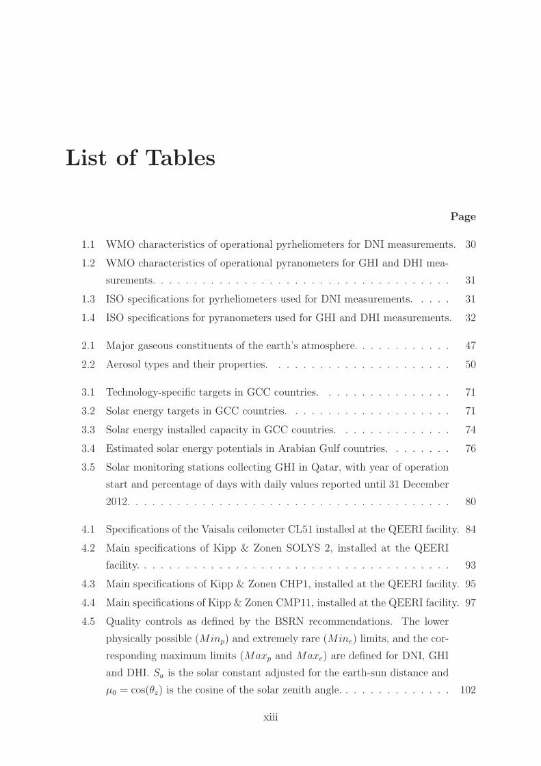
1.1 Left: the sun (photo: NASA/European Space Agency). Right: the earth’s
orbit around the sun (not to scale). . . . . . . . . . . . . . . . . . . . . . 10
1.2 Composite measurements of TSI. . . . . . . . . . . . . . . . . . . . . . . 11
1.3 Spectral distribution of solar radiation at both the top of the earth’s atmo-
sphere and at sea level. Image adapted from Nick84, Wikimedia commons. 12
1.4 Angles used to describe the position of the sun in the sky of an observer
at the earth’s surface. . . . . . . . . . . . . . . . . . . . . . . . . . . . . . 15
1.5 Thermopile principle of operation and illustration of a black/white coating. 21
1.6 Peltier element principle of operation. . . . . . . . . . . . . . . . . . . . . 22
1.7 Examples of photodiode-based sensors from different manufacturers, used
for solar radiation measurements. . . . . . . . . . . . . . . . . . . . . . . 23
1.8 Construction of a typical pyrheliometer. . . . . . . . . . . . . . . . . . . 24
1.9 Absolute cavity radiometer from PMOD/WRC. . . . . . . . . . . . . . . 24
1.10 A typical thermoelectric pyranometer. . . . . . . . . . . . . . . . . . . . 26
1.11 Construction of a silicon photodiode. . . . . . . . . . . . . . . . . . . . . 26
1.12 Spectral response of different pyranometers. . . . . . . . . . . . . . . . . 27
1.13 Rotating Shadowband Radiometer installed at QEERI’s site. . . . . . . . 28
1.14 From PV solar cell to PV solar arrays. Image credit: Florida Solar Energy
Center website. . . . . . . . . . . . . . . . . . . . . . . . . . . . . . . . . 42
1.15 Principle of operation of a PV solar cell. . . . . . . . . . . . . . . . . . . 42
1.16 A liquid flat-plate collector. . . . . . . . . . . . . . . . . . . . . . . . . . 43
1.17 Concentrating collectors. . . . . . . . . . . . . . . . . . . . . . . . . . . . 44
2.1 The major layers within the atmosphere, based on the vertical distribution
and variations of the temperature (red line) in the atmosphere. . . . . . . 46
2.2 Diurnal evolution of the atmospheric boundary layer. . . . . . . . . . . . 49
vii

2.3 Angular dependency of Rayleigh scattering, showing that forward- and
back-scattering intensities are twice as high as those of directions perpen-
dicular to the incident radiation. . . . . . . . . . . . . . . . . . . . . . . . 56
2.4 Example of the angular dependency of Mie scattering intensity, showing
that forward-scattering is much more intense than back-scattering, with
other peaks observed at different angles. . . . . . . . . . . . . . . . . . . 57
2.5 Optic system of a Raman lidar. . . . . . . . . . . . . . . . . . . . . . . . 60
2.6 Photo of the telescope (parabolic solid-glass mirror of 1.8 m diameter) used
by the Barcelona IFAE-UAB team to build their Raman lidar. . . . . . . 61
2.7 Schematic representation of a lidar system’s working principle. . . . . . . 62
3.1 Electricity consumption in Qatar, per capita and per year. . . . . . . . . 69
3.2 Water consumption in Qatar, per capita and per year. . . . . . . . . . . . 70
3.3 Qatar Foundation stadium for the World Cup 2022. . . . . . . . . . . . . 72
3.4 Photovoltaic panels on the roof top of the Qatar National Convention Centre. 73
3.5 Solar Test Facility at Qatar Science & Technology Park. Image courtesy
of Benjamin W. Figgis (QEERI). . . . . . . . . . . . . . . . . . . . . . . 73
3.6 Theoretical space of a solar thermal power plant in North Africa. . . . . 75
3.7 DNI solar maps for Qatar from DLR. . . . . . . . . . . . . . . . . . . . . 77
3.8 DNI solar map of Qatar by SolarGIS model from GeoModel Solar. . . . . 78
3.9 Network of monitoring stations in Qatar, operated by QMD. . . . . . . . 79
3.10 GHI solar map (values in kWh/m2/year) based on daily ground measure-
ments of GHI. . . . . . . . . . . . . . . . . . . . . . . . . . . . . . . . . . 80
4.1 Vaisala Ceilometer CL51, as installed at the QEERI facility in Doha, Qatar. 82
4.2 Vaisala Ceilometer CL51, measurement unit main parts. . . . . . . . . . 83
4.3 Vaisala Ceilometer CL51, optical configuration. Image: Vaisala. . . . . . 84
4.4 Vaisala Ceilometer CL51, principle of operation. . . . . . . . . . . . . . . 85
4.5 Example of a ceilometer measurement signal. . . . . . . . . . . . . . . . . 86
4.6 CL-VIEW cloud and backscatter intensity graphs as measured by the
Vaisala Ceilometer CL51. Data collected on 07/Jun/2013. . . . . . . . . 88
4.7 Samples of backscatter profiles as displayed by BL-VIEW. . . . . . . . . 90
4.8 Solar radiation monitoring station as installed at the QEERI facility in
Doha, Qatar. . . . . . . . . . . . . . . . . . . . . . . . . . . . . . . . . . 92
4.9 Kipp & Zonen CHP1 pyrheliometer used at the solar radiation monitoring
station installed at the QEERI facility. . . . . . . . . . . . . . . . . . . . 94
viii

4.10 Kipp & Zonen CMP11 pyranometers used at the solar radiation monitoring
station installed at the QEERI facility. Note the shadow covering the
sensor of the left pyranometer, in order to measure DHI. . . . . . . . . . 96
4.11 Data logger in its enclosure, for the communication of the solar radiation
measurements from the monitoring station installed at the QEERI facility. 99
4.12 Data analysis of DNI, GHI and DHI measured at the experimental site in
Doha, Qatar, for clear days (9–11 May), cloudy days (7–8 May), with rain
(8 May), with haze (6 May) and days with dust (7–9 June). . . . . . . . 100
5.1 Distance in km to the closest neighbouring station for the QMD ground
stations. . . . . . . . . . . . . . . . . . . . . . . . . . . . . . . . . . . . . 107
5.2 Annual variation of daily GHI averages at Doha International Airport. . 109
5.3 Monthly averages and peaks of global radiation at Doha Airport through-
out the year. . . . . . . . . . . . . . . . . . . . . . . . . . . . . . . . . . . 110
5.4 Daily averages of global radiation at Doha Airport throughout the year. . 111
5.5 Comparison between ground-measured and NASA-derived monthly clear-
ness index at Doha Airport throughout the year. . . . . . . . . . . . . . . 112
5.6 Averages of daily clearness index at Doha Airport throughout the year, for
the period 2008 to 2012. . . . . . . . . . . . . . . . . . . . . . . . . . . . 112
5.7 Sunrise time calculated day by day over a period of one year at the QEERI
site in Doha, Qatar. . . . . . . . . . . . . . . . . . . . . . . . . . . . . . . 115
5.8 Sunset time calculated day by day over a period of one year at the QEERI
site in Doha, Qatar. . . . . . . . . . . . . . . . . . . . . . . . . . . . . . . 115
5.9 1-minute values of solar irradiance, in W/m2, through one year in Doha. 117
5.10 Variation of the beam extraterrestrial solar irradiance in a one-year period. 119
5.11 Variation of the daily extraterrestrial solar irradiation on a horizontal sur-
face at the experimental site in Doha, in a one-year period. . . . . . . . . 120
5.12 Hourly DNI, GHI and DHI in Doha, averaged over one year, from Decem-
ber 2012 to November 2013. . . . . . . . . . . . . . . . . . . . . . . . . . 121
5.13 Hourly DNI, GHI and DHI in Doha, averaged per month, for all the months
in a one-year period, from December 2012 to November 2013. . . . . . . 122
5.14 Daily averages and maximum minute values per day for DNI, GHI and
DHI in Doha in one year, from Dec/2012 to Nov/2013. Values for missing
days are set to negative (see text). . . . . . . . . . . . . . . . . . . . . . . 124
5.15 Monthly averages and maximum daily values per month for DNI, GHI and
DHI in Doha during one year, from December 2012 to November 2013. . 125
ix

5.16 Frequency distributions of one-minute values of solar irradiance through
one year in Doha. All distributions are normalised to 100% for comparison
clarity. . . . . . . . . . . . . . . . . . . . . . . . . . . . . . . . . . . . . . 127
5.17 Monthly clearness index and diffuse ratio in Doha during one year, from
Dec/2012 to Nov/2013. . . . . . . . . . . . . . . . . . . . . . . . . . . . . 128
5.18 Daily clearness index and diffuse ratio in Doha during one year, from
Dec/2012 to Nov/2013. . . . . . . . . . . . . . . . . . . . . . . . . . . . . 130
6.1 Variation of the hourly-averaged backscatter coefficients with height, at
solar noon, for all the clear days through one year in Doha. . . . . . . . . 132
6.2 Cumulative beta in 500-m steps, at solar noon for the clear days of all the
months of the year under study. . . . . . . . . . . . . . . . . . . . . . . . 134
6.3 Average of beta for all clear days of the month versus height, at solar noon.136
6.4 Standard deviation of beta for all clear days of the same month versus
height, at solar noon. . . . . . . . . . . . . . . . . . . . . . . . . . . . . . 138
6.5 Variability of the ratio of range to standard deviation of beta calculated
for all clear days of the same month versus height, at solar noon. . . . . . 140
6.6 Relative variabilities in the day-to-day range of the beta values at noon,
per height intervals of 500 m. Each line corresponds to one month. Winter
includes from October to February, and summer includes the rest of the
year. . . . . . . . . . . . . . . . . . . . . . . . . . . . . . . . . . . . . . . 141
6.7 Frequency distribution of beta in terms of two height bins, at solar noon
for the clear days in the months of January and July. . . . . . . . . . . . 142
6.8 Distributions of beta fitted to noise for each km in height. See details in
text. . . . . . . . . . . . . . . . . . . . . . . . . . . . . . . . . . . . . . . 144
6.9 Goodness of the fit of the beta distribution to a noise distribution for each
km in height. See details in text. . . . . . . . . . . . . . . . . . . . . . . 145
6.10 Daily variation of the zenith angle of the sun around solar noon, from 1
January to 31 December for Doha, Qatar. . . . . . . . . . . . . . . . . . 148
6.11 Daily variation of integrated backscatter around solar noon for cloud-free
days in a one-year period. Non-clear days are shown with Betatot=0. . . 148
6.12 Daily variation of hourly averages of DNI around solar noon for cloud-free
days in a one-year period. Non-clear days are shown with DNI=0. . . . . 149
6.13 Correlation between Kn and integrated backscatter at solar noon in Doha. 150
x

6.14 Comparison of the hourly values of Kn (top) and DNI (bottom) obtained
through the Beta-model vs. the values calculated from DNI measurements,
at the hour from 10 to 11 am (left), and from 12 to 1 pm (right). The
one-to-one line is shown in red. See Tables 6.2 and 6.3 for the statistical
results. . . . . . . . . . . . . . . . . . . . . . . . . . . . . . . . . . . . . . 153
6.15 Comparison of the hourly values of Kn (top) and DNI (bottom) obtained
from SolarGIS vs. the values calculated from DNI measurements, (left) at
the hour from 10 to 11 am and (right) at the hour from 12 to 1 pm. The
one-to-one line is shown in red. See Tables 6.2 and 6.3 for the statistical
results. . . . . . . . . . . . . . . . . . . . . . . . . . . . . . . . . . . . . . 154
6.16 Comparison of the hourly values of Kn (top) and DNI (bottom) obtained
from McClear vs. the values calculated from DNI measurements, (left) at
the hour from 10 to 11 am and (right) at the hour from 12 to 1 pm. The
one-to-one line is shown in red. See Tables 6.2 and 6.3 for the statistical
results. . . . . . . . . . . . . . . . . . . . . . . . . . . . . . . . . . . . . . 155
6.17 (Left) Comparison at the hour from 11 am to 12 pm of the hourly values
of Kn (top) and DNI (bottom) obtained through the Beta-model vs. the
values calculated from DNI measurements, from December 2013 to Novem-
ber 2014. (Right) Same comparison, but for McClear-derived data. The
one-to-one line is shown in red. See Table 6.4 for the statistical results. . 156
6.18 Correlation between Kn and the modified Betatot coefficient, BetaCos, at
solar noon in Doha. . . . . . . . . . . . . . . . . . . . . . . . . . . . . . . 159
6.19 Comparison at two hours: from from 10 am to 11 am (left) and from 12
pm to 1 pm (right) of the hourly values of Kn (top) and DNI (bottom)
obtained through the BetaCos-model vs. the values calculated from DNI
measurements, from December 2012 to November 2013. The one-to-one
line is shown in red. See Tables 6.5 and 6.6 for the statistical results. . . 160
6.20 Comparison at the hour from 11 am to 12 pm of the hourly values of Kn
(left) and DNI (right) obtained through the BetaCos-model vs. the values
calculated from DNI measurements, from December 2013 to November
2014. The one-to-one line is shown in red. See Table 6.7 for the statistical
results. . . . . . . . . . . . . . . . . . . . . . . . . . . . . . . . . . . . . . 161
6.21 Correlation between Kn and the modified Betatot coefficient BetaCos for
all the clear days from 7 am to 4 pm, for the period Dec/2012 to Nov/2013
in Doha. . . . . . . . . . . . . . . . . . . . . . . . . . . . . . . . . . . . . 163
xi

6.22 Comparison of the hourly values of Kn (left) and DNI (right) obtained
through the BetaCos-model (top figures) and the McClear model (bottom
figures) vs. the values calculated from DNI measurements, from December
2013 to November 2014, for hours 8 to 16 (from 7:01 to 16:00). The one-
to-one line is shown in red. See Table 6.8 for the statistical results. . . . 163
6.23 Study of the performance of the McClear model represented by the ratio
DNIMcClear/DNIground, vs. Betatot, at the hour from 11 am to 12 pm,
where DNIMcClear and DNIground are, respectively, the hourly values of
DNI obtained from McClear and calculated from DNI measurements. . . 165
6.24 Fit applied to the performance of the McClear model for Betatot values
exceeding 70000 · [105 srad · km]−1. . . . . . . . . . . . . . . . . . . . . . 166
6.25 Validation of the calibration of the McClear model, at the hour 11 am,
from 10 to 11 am. On the left, the uncalibrated DNI ratio; on the right,
the same ratio after correcting the McClear DNI. . . . . . . . . . . . . . 167
6.26 Validation of the calibration of the McClear model, at the hour 1 pm, from
12 to 1 pm. On the right, the uncalibrated DNI ratio; on the left, the same
ratio after correcting the McClear DNI. . . . . . . . . . . . . . . . . . . . 167
8.1 Beta values for each hour from 6 am to 6 pm, averaged by month (thin
dashed lines) and by season (winter and summer, thicker lines), for the
new selection of clear days, from December 2012 to November 2013. . . . 174
8.2 Hourly values of measured Kn vs. Betatot from 8 am to 4 pm for the
new selection of clear days, from December 2012 to November 2013. For
illustration purposes only, the red line representing the Kn values derived
from the Beta-model is also shown. . . . . . . . . . . . . . . . . . . . . . 175
8.3 Hourly variations of K ′n (top) and Kn (bottom) through the day, for the
new selection of clear days from December 2012 to November 2013. . . . 176
xii
List of Tables
Page
1.1 WMO characteristics of operational pyrheliometers for DNI measurements. 30
1.2 WMO characteristics of operational pyranometers for GHI and DHI mea-
surements. . . . . . . . . . . . . . . . . . . . . . . . . . . . . . . . . . . . 31
1.3 ISO specifications for pyrheliometers used for DNI measurements. . . . . 31
1.4 ISO specifications for pyranometers used for GHI and DHI measurements. 32
2.1 Major gaseous constituents of the earth’s atmosphere. . . . . . . . . . . . 47
2.2 Aerosol types and their properties. . . . . . . . . . . . . . . . . . . . . . 50
3.1 Technology-specific targets in GCC countries. . . . . . . . . . . . . . . . 71
3.2 Solar energy targets in GCC countries. . . . . . . . . . . . . . . . . . . . 71
3.3 Solar energy installed capacity in GCC countries. . . . . . . . . . . . . . 74
3.4 Estimated solar energy potentials in Arabian Gulf countries. . . . . . . . 76
3.5 Solar monitoring stations collecting GHI in Qatar, with year of operation
start and percentage of days with daily values reported until 31 December
2012. . . . . . . . . . . . . . . . . . . . . . . . . . . . . . . . . . . . . . . 80
4.1 Specifications of the Vaisala ceilometer CL51 installed at the QEERI facility. 84
4.2 Main specifications of Kipp & Zonen SOLYS 2, installed at the QEERI
facility. . . . . . . . . . . . . . . . . . . . . . . . . . . . . . . . . . . . . . 93
4.3 Main specifications of Kipp & Zonen CHP1, installed at the QEERI facility. 95
4.4 Main specifications of Kipp & Zonen CMP11, installed at the QEERI facility. 97
4.5 Quality controls as defined by the BSRN recommendations. The lower
physically possible (Minp) and extremely rare (Mine) limits, and the cor-
responding maximum limits (Maxp and Maxe) are defined for DNI, GHI
and DHI. Sa is the solar constant adjusted for the earth-sun distance and
μ0 = cos(θz) is the cosine of the solar zenith angle. . . . . . . . . . . . . . 102
xiii

4.6 Quality controls as defined by the BSRN recommendations for the com-
parison tests. θz is the solar zenith angle and sum is DNI · cos(θz) +DHI.103
5.1 Annual means of daily GHI for Doha International Airport, and the cor-
responding number of days with non-missing daily GHI values. . . . . . . 109
5.2 Annual averages of clearness index for Doha and other cities; (a) 5-year
average of ground measurements, and year by year, (b) 22-year averages
by NASSA-SSE, and (c) 1-year ground measurements, 2007. . . . . . . . 113
5.3 Number of entries which fail the physically possible limits (phys) and ex-
tremely rare limits (ext) tests, and the total number of collected entries in
each solar zenith angle (SZA) interval. . . . . . . . . . . . . . . . . . . . 116
5.4 Number of entries which fail the comparison tests: the comparison among
the three components and the diffuse ratio test. The total number of
collected entries within every solar zenith angle (SZA) cut is also shown. 116
5.5 Comparison of monthly averages of GHI in Doha, in kWh/m2/day: based
on one year of data collected by the QEERI solar station and 5 years of
data collected by the QMD station. . . . . . . . . . . . . . . . . . . . . . 126
6.1 Validations of the different models with ground measurements. . . . . . . 152
6.2 Statistical indicators of the comparison of modelled against measured Kn
(dimensionless) and DNI (W/m2), at the hour from 10 to 11 am, from
Dec/2012 to Nov/2013. rMBE and rRMSE are in %. . . . . . . . . . . . 157
6.3 Statistical indicators of the comparison of modelled against measured Kn
(dimensionless) and DNI (W/m2), at the hour from 12 to 1 pm, from
Dec/2012 to Nov/2013. rMBE and rRMSE are in %. . . . . . . . . . . . 157
6.4 Statistical indicators of the comparison of modelled against measured Kn
(dimensionless) and DNI (W/m2), at the hour from 11 am to 12 pm, for
the data set of the period December 2013 to November 2014. rMBE and
rRMSE are in %. . . . . . . . . . . . . . . . . . . . . . . . . . . . . . . . 158
6.5 Statistical indicators of the comparison of modelled against measured Kn
(dimensionless) and DNI (W/m2), at the hour from 10 am to 11 am, for
the data set of the period December 2012 to November 2013. rMBE and
rRMSE are in %. . . . . . . . . . . . . . . . . . . . . . . . . . . . . . . . 161
6.6 Statistical indicators of the comparison of modelled against measured Kn
(dimensionless) and DNI (W/m2), at the hour from 12 to 1 pm, for the data
set of the period December 2012 to November 2013. rMBE and rRMSE
are in %. . . . . . . . . . . . . . . . . . . . . . . . . . . . . . . . . . . . . 161
xiv

6.7 Statistical indicators of the comparison of modelled against measured Kn
(dimensionless) and DNI (W/m2), at the hour from 11 am to 12 pm, for
the data set of the period December 2013 to November 2014. rMBE and
rRMSE are in %. . . . . . . . . . . . . . . . . . . . . . . . . . . . . . . . 162
6.8 Statistical indicators of the comparison of modelled against measured Kn
(dimensionless) and DNI (W/m2), at the hours from 7 am to 4 pm, for
the data set of the period December 2013 to November 2014. rMBE and
rRMSE are in %. . . . . . . . . . . . . . . . . . . . . . . . . . . . . . . . 164
6.9 Statistical indicators of the comparison of McClear against McClear cali-
brated using the Betatot coefficient, for the data set of the period December
2013 to November 2014, for the hours 11 am and 1 pm. rMBE and rRMSE
are in %. . . . . . . . . . . . . . . . . . . . . . . . . . . . . . . . . . . . . 167
xv

xvi

Abbreviations
ABL Atmospheric Boundary Layer
ACR Active Cavity Radiometer
ACRIM Active Cavity Radiometer Irradiance Monitor
AOD Aerosol Optical Depth
ARF Aerosol Radiative Forcing
AU Astronomical Unit
AWS Automatic Weather Stations
BHI Beam Horizontal Irradiance
BL Boundary Layer
BSRN Baseline Surface Radiation Network
CERES Clouds and the Earth’s Radiant Energy System
CPV Concentrated Photovoltaic
CSP Concentrated Solar Power
DHI Diffuse Horizontal Irradiance
DNI Direct Normal Irradiance
ERBS Earth Radiation Budget Satellite
FOV Field Of View
GCC Gulf Cooperation Council
GHI Global Horizontal Irradiance
GMT Greenwich Mean Time
HA Hour Angle
IRENA International Renewable Energy Agency
ISO International Standards Organization
LIDAR LIght Detection And Ranging
LST Local Solar Time
LSTM Local Standard Time Meridian
LT Local Time
MBE Mean Bias Error
xvii

MISR Multi-angle Imaging SpectroRadiometer
MODIS MODerate resolution Imaging Spectroradiometer
NASA National Aeronautics and Space Administration
PBL Planetary Boundary Layer
PMOD Physikalisch-Meteorologisches Observatorium Davos
PV Photovoltaic
QEERI Qatar Environment and Energy Research Institute
QMD Qatar Meteorological Department
QNFSP Qatar National Food Security Programme
RMSE Root Mean Square Error
SoHO Solar and Heliospheric Observatory
SORCE SOlar Radiation and Climate Experiment
TIM Total Irradiance Monitor
TSI Total Solar Irradiance
TCTE TSI Calibration Transfer Experiment
TST True Solar Time
UTC Universal Time Coordinated
WCRP World Climate Research Programme
WMO World Meteorological Organisation
WRC World Radiation Center
WRDC World Radiation Data Center
xviii

Introduction
The electromagnetic radiation emitted by the sun is a crucial source of energy on the
earth’s surface, playing an important role in the weather, climate and different biological
processes on earth. The earth’s atmosphere affects the amount of solar radiation that
reaches the surface of the planet, due to absorption and scattering. This results in
changing the amount and characteristics of the solar radiation available at ground level:
the solar radiation reaching a horizontal surface, called global horizontal irradiance (GHI),
is composed of the radiation coming directly from the sun disk, known as direct or beam
irradiance, and the scattered or diffuse irradiance, coming from the sky dome. These
components can be harvested by different technologies, to produce heat or electricity.
The direct component is the main gauge of projects based on concentrating technologies
such as concentrated solar power (CSP) and concentrated photovoltaic (CPV), while GHI
is the required parameter for photovoltaic (PV) projects. Being the fuel of such systems
and an important parameter for climate and atmospheric studies, it is vital to conduct
an accurate assessment of the solar resources available at ground level. This allows for
reliable planning and implementation of solar energy-based projects, and also provides
precious information for any other scientific or technical fields requiring the study and
analysis of solar radiation.
Of particular interest to this work is the direct component of the solar radiation
emanating directly from the sun disk and reaching the earth’s surface on a plane normal
to the sun rays, called DNI, the direct normal irradiance. The amount of DNI at ground
level is affected by:
• the amount of incoming radiation at the top of the atmosphere, which depends on
the sun-earth distance and varies around 6.7% between the closest and the farthest
points;
• the distance traversed by the sun rays from the top of the atmosphere to the ground
level, that is, the air mass or thickness of the atmosphere along the path of the sun
rays to the ground;
1

2
• the atmospheric constituents that intercept the solar radiation along its path, scat-
tering and absorbing part of it, thus reducing its magnitude on the ground level.
Due to these dependencies, the direct solar radiation is more abundant in regions
with these characteristics: low latitudes, long sunshine durations, clear or cloudless skies
most of the time, i.e., small cloud cover, and obviously, clean sky conditions, that is, low
pollution and low levels of aerosols in the atmosphere.
The main objective of this research work is to accurately measure the solar radiation
in Doha, Qatar, and to show how the atmospheric conditions, in a region located at low
latitudes, can attenuate the direct solar radiation reaching the earth surface. Indeed,
Qatar has, on daily basis, long hours of sunshine and usually the sky is cloudless most of
the year. However, the high amounts of aerosols present in the atmosphere, whether of
natural or anthropogenic nature, have a definite effect on the direct solar radiation, which
shows values lower than what could be expected in such a region of the world. In this
work, the effect of aerosols on the direct component of the solar radiation is quantified
by the use of a lidar-ceilometer device which measures the backscatter profiles of the
atmosphere. The comparison of backscatter and solar radiation measurements constitutes
the essence of this work, and demonstrates that lidar-ceilometer devices, normally used
for determining cloud heights or boundary layer heights in the atmosphere, can also be
considered as prospective tools for aerosol estimation in the solar resource assessment
field.
Research context
Given its geographic location, in the Sun Belt region of the world, Qatar has plenty of
solar radiation resources: sunny conditions most of the time with an average sunshine
duration of 9.2 hours per day and limited cloud cover during the year [1]. The country has
already set several plans and targets for harvesting solar energy as an alternative to fossil
fuels, a solution for diversifying its energy resources and reducing its carbon emissions
[2].
To efficiently use the solar resource, it is essential to perform an estimation of the
available solar radiation and evaluate its spatial and temporal variabilities. This can
be done in terms of solar maps, which provide a clear representation on grid cells of
the spatial variations of solar radiation in a country or a region. Such solar maps can
assist and guide in the process of setting national solar energy targets, based on realistic
figures of the resources. In addition, this will play a major role in selecting the most
appropriate technology, qualifying a site, and optimising the design of solar power plants.

3
When it comes to the implementation and deployment of utility-scale solar energy-based
projects, more in-depth assessment of solar resources and site-specific data are crucial.
This assessment constitutes the primary step and includes the precise knowledge of the
available solar energy at the site and over time. Apart from energy production, solar
radiation data is needed in other fields such as atmospheric sciences, climate change
studies, meteorology, etc.
An accurate method for characterising the solar radiation is through the use of high
quality ground measurements of solar radiation. A sufficient number of ground stations
measuring DNI, GHI and DHI (diffuse horizontal irradiance) over the whole area of
interest and for at least one complete solar cycle of 11 years is ideally required for this
purpose. In practice, however, this is usually not possible and is not the case in most
areas of the world. The alternative solution is to use reliable long-term satellite-derived
solar radiation data validated against ground measurements in the region, and combine
it with short-term ground-measured solar radiation data, if available [3].
The existing satellite-based solar maps for Qatar, described in Section 3.3, are in-
formative and give a first insight on the availability of solar radiation in the country.
However, their reliabilities have not been assessed with ground-measured solar radiation
data in Qatar. Global solar radiation has been measured in several locations in the coun-
try since 2007. These GHI data samples are of unknown quality, but if filtered with
quality control checks, they can be considered of value to validate or calibrate the mod-
elled global solar radiation. Yet, ground-measured DNI data are not available for Qatar
and the only available DNI data are derived from satellite observations. A serious prob-
lem of the modelled DNI is the disagreement between the different available databases,
leading to high uncertainties. In Europe, for instance, relative standard deviations of
17% have been found between different datasets of modelled DNI data [4]. The evaluated
differences between modelled datasets can reach as much as approximately 30% in many
regions, as stated in [5]. Indeed, by its nature, being the component of solar radiation
that arrives to the earth’s surface directly from the sun, DNI is highly influenced by the
atmospheric contents along its path, i.e., small changes of the atmospheric conditions
have a strong influence on its attenuation. This fact adds more challenges to achiev-
ing high accuracy and low uncertainty in DNI modelling, given the constantly changing
atmospheric conditions.
In a clear sky, the more radiatively active atmospheric constituents are aerosols, water
vapour and ozone. Aerosols are the main contributor to the extinction of the direct
beam [6]. Their concentrations exhibit large variation in space and time. Errors in the
determination of aerosol data give uncertainties in the order of 15 to 20% on a mean

4
annual basis in satellite-derived DNI [7]. Therefore, accurate aerosol determination is
critical for modelling the direct component of solar radiation.
In general, the extinction factor due to aerosols is represented by the aerosol optical
depth (AOD) parameter, which is a measure of the total extinction of sunlight over the
vertical path, as it passes through the atmosphere. Commonly, AOD is either deter-
mined by spectral solar attenuation of sunphotometer measurements [8], or estimated
using satellite sensors [9, 10], or modelled using chemical-transport models [11]. The
ground-based data present the most accurate option for AOD determination. However,
they are generally limited in spatial and temporal coverage. Satellite observations, in
contrast, provide long-term and uninterrupted spatial coverage, but they provide data
with lower spatial and temporal resolutions and show high uncertainties when compared
to ground measurements [12], specially over regions with high dust and aerosol loads [13].
In addition, several studies show significant differences between the data sets produced
by the different sources, a factor which presents a particular challenge in the estimation
of the direct component of solar radiation [14].
In order to summarise the current situation and put things into perspective, the
major points to retain are listed below. From this list it is easy to define and prioritise
the research opportunities:
• Qatar is considered a potentially good location for solar energy-based projects in
general, and CSP systems in particular, since it is located at low latitudes and has
long hours of sunshine and low cloudiness most of the time.
• DNI being the fuel of CSP, there is a need to have accurate and reliable data of
DNI for project planning, design and implementation.
• Ground-measured DNI data is so far not available, and the only option is to rely
on modelled DNI data.
• Differences exist between modelled DNI datasets from different sources, see Section
1.5 for some available databases.
• The main input parameter affecting the modelled DNI in clear-sky conditions is
aerosol data.
• AOD is normally used to describe the solar radiation extinction due to aerosols.
• Ground data of AOD are generally scarce, and unavailable for Qatar.
• AOD data derived from satellite observations or chemical transport models show
discrepancies and high uncertainties.

5
• The uncertainties are even more accentuated in extreme atmospheric conditions,
such as those in Qatar, characterised by high aerosols loads.
In view of the above-mentioned points, it was deemed necessary to address these
challenges in a direct and concise manner, covering these gaps, which are particular to
the region under study, while developing a research concept that can be applicable to
other regions.
To that end, this thesis work presents an analysis of the characteristics of solar radia-
tion and backscatter profiles of the atmosphere in Doha, Qatar. It introduces a new model
to derive DNI in clear sky conditions from lidar-ceilometer measurements. It also tackles a
new approach of evaluating local aerosol data from the backscatter profile measurements,
which can be ultimately used in solar radiation modelling. This analysis was possible
through: the study of one year of measurements with a high-quality solar radiation mon-
itoring station collecting the three components of solar radiation (DNI, GHI and DHI)
at 1-minute temporal resolution, and the measurements of a lidar-ceilometer pointing
vertically upwards and profiling with high temporal resolution (36 s) the backscattering
properties of the atmosphere. The model for DNI derivation was developed by combin-
ing DNI and backscatter measurements, where aerosol information was represented by
the integration of the backscatter signal of the lidar-ceilometer over the vertical column.
This new suggested model for DNI retrieval has been evaluated and the results have been
compared with those of satellite models and shows good, and in some cases even better,
results. An important application emerged from the suggested analysis, and consists of
using the lidar signal to indirectly calibrate AOD retrieval methods. This is important to
elucidate the limitation of DNI models in extreme conditions of high aerosol loads. The
retrieval of aerosol data from backscatter measurements presents high temporal resolution
(hourly, as opposed to daily or monthly-averaged AOD data) and high spatial resolution
(local measurements, in contrast to a minimum of 100×100 km2 grid cells generally used
in solar radiation modelling). Local measurements allow to capture the high spatial and
temporal variability of aerosols, a feature of high importance when modelling aerosols in
a country like Qatar. Indeed, large amounts of aerosols are present in the atmosphere of
Qatar and dust storms can strike suddenly, making significant changes in the local aerosol
regime. Thus, the use of aerosol data as derived from the ceilometer could present an
alternative for solar radiation modelling or satellite data calibration, in regions prone to
dust and aerosols.
Through the correlation study of the direct normal irradiance with the backscatter
profiles of the atmosphere over Doha, Qatar, it is demonstrated here that apart from its
normal use for cloud and boundary layer monitoring, lidar-ceilometer devices can also be

6
ultimately used for deriving DNI and for calibrating satellite- and model-derived DNI.
The radiative effect of aerosols, instead of being presented by the usual AOD parameter,
is evaluated by the integration of the backscatter signal of the lidar-ceilometer over the
vertical column. This method, although promising, is still yet to be validated and consol-
idated with more data and, most importantly, should be derived with a more physically
sound approach, a concept guiding the future perspectives of this thesis work.
Thesis outline
The thesis work, as highlighted and presented in this introduction, is divided as per the
following structure:
• Chapter 1 - Overview on Solar Radiation.
Within this chapter, solar radiation at the top of the atmosphere, the effects of
the earth’s atmosphere on the attenuation of solar radiation, and solar radiation
components at the ground level are discussed. Methods of measuring and mod-
elling solar radiation are also described with examples of use of solar radiation as a
renewable source of energy.
• Chapter 2 - Atmospheric Properties and Lidar Techniques.
This chapter briefly introduces the atmospheric structure and properties with fur-
ther description of the troposphere, its Atmospheric Boundary Layer (ABL) and
the influence of aerosols on the earth’s radiation budget. Light-matter interaction
within the atmosphere is shortly discussed along with the theories of interactions
of molecules and particles with light (Rayleigh and Mie theories, respectively). De-
scriptions of the lidar technique and the elastic backscatter lidar are also given.
• Chapter 3 - Solar Energy in Qatar.
Qatar’s geographic location and climate along with the plans for the introduction of
solar radiation in the energy production mix of the country is briefly discussed in this
chapter. The existing solar maps and solar resource assessment efforts undertaken
in Qatar are also presented.
• Chapter 4 - Instrumentation.
The experimental setup used in this thesis work is shown here, including descriptions
of the ceilometer used for the measurement of the backscatter coefficient of aerosols
in the atmosphere, the solar radiation monitoring station used for the measurements
of solar radiation, and their respective data acquisition systems.

7
• Chapter 5 - Solar Radiation Data Analysis.
The analysis of historical global solar radiation data is shown first in this chapter.
The analysis of one year of solar radiation measured at the experimental site is
then presented. This includes the hourly, daily and monthly averages as well as
frequency distributions of solar irradiance values. The atmospheric conditions of
the site are also studied through two indices: the clearness index and diffuse ratio.
• Chapter 6 - Correlation of DNI with backscatter.
This chapter is mainly dedicated to present the method and results of the correlation
between the lidar backscatter and solar radiation measurements. This includes first
the analysis used to find the atmospheric height used for the integration of the
backscatter signal. The methodology for the correlation is then described along
with the validation of the proposed model and an example of application using
the aerosol information extracted from lidar measurements for the calibration of
satellite-derived solar data.
• Chapter 7 - Conclusions.
Conclusions about the main results found in this thesis work are summarised in
this chapter.
• Chapter 8 - Future work.
Perspectives are discussed here with potential expansion of the work for a better
application and use of the presented results.

8

Chapter 1
Overview on Solar Radiation
This chapter provides insight on the key characteristics of solar radiation. It discusses
the basic definition of solar radiation, the effects of the earth’s atmosphere on the trans-
mission of solar radiation, and solar radiation components at ground level. It also covers
most aspects of solar radiation measurement methods, comprising a description of the
radiometric sensors and their principles of operation. A brief discussion of the setup and
operation of a solar radiation monitoring station is presented. Also outlined, are meth-
ods of solar radiation modelling as well as the use of satellite images for solar radiation
estimation. Finally, the use of solar energy as a clean and renewable energy source is
addressed, with examples of its application.
1.1 Introduction to solar radiation
The sun is the fundamental source of almost all the energy on earth and the main driver
of its climate system. Solar radiation emanating from the sun constitutes a crucial com-
ponent of the earth’s global energy balance and drives different systems, such as the
atmospheric and hydrological processes. According to a NASA facts document [15], ev-
ery square metre on earth receives approximately, on average over a year, 342 W of solar
energy, equivalent to a power of 4.4×10¹⁶ W for the whole planet (excluding waters). To
put this number in perspective, about 44 million large (1×10⁹ W ) electric power plants
are needed to equal this amount of energy.
The sun is a star, basically a ball of gas composed of about 92% hydrogen (H2) and
about 8% helium (He). It has a surface temperature of around 5000 K, with its core
reaching between 8 and 40 million K [16]. Due to the high temperatures and pressures
in its interior, nuclear fusion reactions occur, causing it to emit enormous amounts of
electromagnetic radiation that travels into space at the speed of light. The earth is the
9
10 CHAPTER 1. OVERVIEW ON SOLAR RADIATION
third closest planet to the sun, at a mean distance of around 150 million kilometres,
completing an elliptical orbit, with small eccentricity, in about 365 days.
Figure 1.1: Left: the sun (photo: NASA/European Space Agency). Right: the earth’s
orbit around the sun (not to scale).
The electromagnetic radiation emitted by the sun ranges from very-short-wavelength
gamma rays to long-wavelength radio waves in the electromagnetic spectrum, with a
dominant portion emitted in the visible range around 0.48 μm. The total amount of solar
radiation, integrated over all wavelengths, received on a plane perpendicular to the sun’s
rays at the top of the earth’s atmosphere, at the mean sun-earth distance of 1 astronomical
unit (AU), is called the extraterrestrial solar irradiance, usually referred to as the total
solar irradiance (TSI), previously known as solar constant. Measurements of TSI from
space-borne instruments in the late 1970s indicate that TSI varies over time and presents
periodic components, the main one being the 11-year solar cycle (or sunspot cycle). The
Active Cavity Radiometer Irradiance Monitor-I (ACRIM-I) was the first instrument, in
1979, to show that the total solar irradiance from the sun is not a constant. From 1984 on,
TSI has also been measured by the Earth Radiation Budget Satellite (ERBS) instrument.
Second and third ACRIM instruments have also been measuring TSI, in addition to
the VIRGO on the NASA/ESA Solar and Heliospheric Observatory (SoHO). The SOlar
Radiation and Climate Experiment (SORCE) satellite, launched in 2003, continues to
produce TSI measurements through the Total Irradiance Monitor (TIM). More recently,
the TSI Calibration Transfer Experiment (TCTE) instrument was launched into orbit in
2013, and has been providing TSI data since December 2013.
Different composite records of TSI are available and differ in their absolute scale and
temporal variations due to calibration and degradation problems of spaceborne radiome-
ters. Figure 1.2 shows, for instance, the most recent version (as of this writing) of the
composite provided by the ‘Physikalisch-Meteorologisches Observatorium Davos’ of the
World Radiation Center (PMOD/WRC), compared with two other composites [17]. The

1.1. INTRODUCTION TO SOLAR RADIATION 11
composites present space-based measurements of TSI since 1980, normalised to 1 AU and
covering three and a half 11-year solar cycles.
1980 1985 1990 1995 2000 2005 2010 2015
1364
1366
1368
1980 1985 1990 1995 2000 2005 2010 2015
a) PMOD Composite 42_64_1502 (org. VIRGO scale)
HF HFACRIM−I ACRIM−II VIRGO
1980 1985 1990 1995 2000 2005 2010 2015
1358
1360
1362
b) ACRIM Composite
HF HFACRIM−I ACRIM−II ACRIM−III
Minimum 22−23Minimum 23−24
1980 1985 1990 1995 2000 2005 2010 2015
1364
1366
1368
c) IRMB Composite
HF HFACRIM−I ACRIM−II DIARAD IRMB
Tot
al S
olar
Irra
dian
ce (
Wm
−2 )
Figure 1.2: Composite measurements of TSI based on satellite-based radiometers (colour-
coded) and model results produced by the World Radiation Center and two other com-
posites, showing TSI variations for three solar cycles [17].
The typical variation in annual mean TSI is estimated to be around 0.1% between
the minimum and the maximum of the 11-year cycle of the sun due to changing numbers
and strength of sunspots and other phenomena, depending on solar activity. In general,
this variation is stable and is considered negligible, so the term ‘solar constant’ is given
to a long-term average of the TSI. The World Meteorological Organisation (WMO) has
recommended a solar constant value of 1367 W/m2. The American Society for Testing
and Materials (ASTM) gives the value of 1366.1 W/m2 to the solar constant, based on 25
years of data [18]. Gueymard, in a study in 2004 [18], reported that TSI measurements
have an inherent absolute uncertainty of at least 0.1%, or 1.4 W/m2, and he confirmed in
the same study a solar constant value of 1366.1 W/m2. Therefore, it can be assumed that
the differences between the measured TSI values given above were not of high significance.
More recently, measurements of the SORCE satellite indicate a slightly lower value, of
approximately 1361 W/m2 [19].
In the following chapters of this work, the TSI given by I0 = 1367 W/m2 has been

12 CHAPTER 1. OVERVIEW ON SOLAR RADIATION
used, as recommended by the WMO. TSI, or solar constant, as discussed above, refers to
the solar radiation flux at the top of the atmosphere at the mean value of the sun-earth
distance, R0, of 1 AU. However, since the distance R between the sun and the earth varies
during the year by 1.67% from their mean separation, the solar radiation flux at the top
of the atmosphere, DNI0, varies during the year over a range of about 6.7% (inversely
proportional to the square of the distance from the sun). The correction factor is related
to the eccentricity of the earth’s orbit, and is given by the following equation:
DNI0I0
=
(R0
R
)2
∼ 1 + 0.033 cos
(2πn
365
), (1.1)
where n is the day of the year, from 1 to 365. In the literature, other approximation
equations can be found, some more accurate, some less. For instance, the one given by
Spencer in terms of a Fourier series expansion is more accurate. However, Equation 1.1
is considered accurate enough for most applications of solar resource assessment, and is
used in the current work [16].
The spectral distribution of the extraterrestrial solar radiation is shown in Figure 1.3
(yellow curve). This distribution is similar to that of a black body with a temperature
of 5778 K, with a spectral range of about 300 to 4000 nm, referred to as the short-wave
solar radiation. The integrated energy over the same region is the broadband or total
solar radiation.
Figure 1.3: Spectral distribution of solar radiation at both the top of the earth’s atmo-
sphere and at sea level. Image adapted from Nick84, Wikimedia commons.

1.2. SOLAR RADIATION AT THE EARTH’S SURFACE 13
1.2 Solar radiation at the earth’s surface
The amount of incoming solar radiation at the earth’s surface is affected by the atmo-
spheric composition, which intercepts the radiation along the way from the top of the
atmosphere to the surface. As will be seen in Chapter 2, the atmosphere contains about
78% nitrogen, 21% oxygen and 1% argon in its lowest part. Other trace gases and water
vapour are also found in low concentrations, but have a large influence on the radiation
budget. A thin layer of ozone is present in the stratosphere and has a major role in
the absorption of the ultraviolet wavelengths. In addition, atmospheric aerosol particles
whether of natural sources such as dust, sea-salt spray, biological decay, chemical reactions
of atmospheric gases, etc. or anthropogenic, i.e., human-induced such as from agricul-
ture, transport, industrial emissions, etc., have a high impact on solar radiation. After
penetrating the earth’s atmosphere, the extraterrestrial solar radiation encounters these
atmospheric constituents and its intensity is attenuated due to scattering and absorption
processes that take place on its path before reaching the ground.
Scattering is due to radiation interaction with air molecules, water vapour and aerosols.
It depends on the number of particles and the size of the particle relatively to the wave-
length. Air molecules, for instance, scatter radiation as described by the Rayleigh theory,
more significantly at shorter wavelengths, i.e., the ultraviolet and visible ranges, and
there is little scattering in the infrared range, see Section 2.2.1. For larger particle sizes,
such as dust and water vapour, the scattering process is more complex. For these cases,
the Mie theory is applied. It describes the scattering of radiation by sphere-shaped ob-
jects, see Section 2.2.1. A different approach commonly used to explain the process of
scattering by aerosols is described by the Angstrom turbidity equation [16], which gives
the atmospheric turbidity and its wavelength dependence:
τa,λ = exp(−βλ−αm), (1.2)
where τa,λ is the transmission function, β is the Angstrom turbidity coefficient, depending
on the aerosol loading in the atmosphere and typically ranging between 0 (very clean
atmosphere) and 0.4 (high aerosol amounts) [20], α is the wavelength exponent and
depends on the size distribution of the aerosols, λ is the wavelength of the radiation in
micrometres andm is the air mass along the path of the radiation, that is, the path length
that solar radiation takes through the atmosphere normalised to the shortest possible path
length when the sun is directly overhead.
Absorption of solar radiation is selective and is mostly due to ozone, water vapour
and carbon dioxide in the atmosphere. Ultraviolet radiation is mainly absorbed by ozone,

14 CHAPTER 1. OVERVIEW ON SOLAR RADIATION
but also by sulphur dioxide, nitrogen dioxide and trace gases. In the visible range, there
is little absorption. Water vapour and carbon dioxide absorb strongly the solar radiation
in the infrared range.
All these wavelength-dependent processes change the spectrum of the radiation that
reaches the ground. For instance, the extraterrestrial radiation reaching the outer atmo-
sphere at solar zenith angle of zero (see Section 1.2.1), decreases by about 30% on a very
clear day to nearly 90% on a very cloudy day. The typical spectral distribution of the
radiation at the earth’s surface is shown by the red curve of Figure 1.3. Approximately
half of the solar radiation at ground level is in the visible portion of the spectrum. The
attenuation of the extraterrestrial solar radiation below 300 nm is mainly caused by the
absorption by the ozone layer present in the stratosphere. The attenuation in the visible
range is mainly due to Rayleigh and Mie scattering by gas molecules. Several strong
absorption bands are seen in the infrared region of the spectrum due to water vapour
and CO2, which are responsible for the absorption of all solar radiation above 2500 nm.
The spectrum of the solar radiation at the earth’s surface depends upon the changing
characteristics of the atmosphere, the surface composition, location, solar zenith angle
and the air mass from the top of the atmosphere to the ground.
1.2.1 Sun position and sun angles
For the vital task of calculating the solar radiation intensity on any specified point on
earth, it is necessary to know not only the properties of the atmosphere, but also the
position of the sun in the sky, for any location on earth, at any time of the day. Two
movements govern the variations of the sun’s position in the sky:
• The earth’s rotation around its axis, which modulates the variations through the
day, from sunrise to sunset.
• The earth’s revolution around the sun in an elliptic orbit, which modulates the
variations through the year.
Moreover, the tilt of the earth’s axis of rotation, as well as the geographic latitude of
the location of interest, play an important role in calculating the position of the sun in
the sky.
In order to find the sun’s position for a given point on earth at a given time, several sun
angles can be defined using different coordinate systems. Given that the sun’s position
needs to be known on the ‘sky dome’ seen by an observer on the surface of the earth,
as shown in Figure 1.4, it is convenient to use a spherical coordinate system, with the
observer’s location as the origin of the coordinates.

1.2. SOLAR RADIATION AT THE EARTH’S SURFACE 15
NS
E
W
Azimuth
Zenith
Sun
Normal toground
Figure 1.4: Angles used to describe the position of the sun in the sky of an observer at
the earth’s surface.
The radial distance to the sun is used to retrieve the solar radiation value at the
top of the earth’s atmosphere, using Equation 1.1. What remains to be determined are
two coordinates, i.e., the position of the sun on the imaginary hemispherical surface of
the sky dome, given by the azimuth and zenith angles. The azimuth angle indicates in
which cardinal direction the sun is located, like a compass direction, with North as the
reference, and varying between 0◦ and 360◦. The zenith angle is measured between the
vertical overhead and the line to the centre of the sun, and is the complement of the solar
elevation angle (elevation of the sun from the horizontal). However, for the purposes
of this thesis work, only the zenith angle and the radial distance to the sun are needed
and discussed here. The solar zenith angle at any moment and location is interrelated
by trigonometric relationships with a number of other angular quantities that take into
account the location, time of the day, and time of the year. The solar zenith angle, θz,
as used in this thesis work, is estimated using the following expression:
cos(θz) = sinφ · sin δ + cosφ · cos δ · cos(ha), (1.3)
where φ is the latitude of the location of interest, on earth (-90 to 90 degrees), δ is the
declination angle of the sun, and ha is the hour angle of the sun.
16 CHAPTER 1. OVERVIEW ON SOLAR RADIATION
The sun’s declination and hour angle describe the movement of the sun in the sky due
to the earth’s rotation and translation, and are more conveniently defined in an equatorial
coordinate system (with origin at the earth’s centre and projecting the earth’s equator
onto the celestial sphere). This system is independent from the position of the observer
on earth but depends on the time of observation.
• The hour angle (ha) is the conversion of the true solar time (tst) into an angle in
degrees corresponding to the angular motion of the sun along its path in the sky.
The solar time is the apparent time and path of the sun in the sky relative to a
specified location on earth. Solar time is different from the local time due to the
orbital eccentricity of the earth and human adjustments such as time zones and
daylight savings. Solar noon is when the sun is in its highest position in the sky.
The hour angle is 0◦ at solar noon and each hour away from solar noon corresponds
to a movement of the sun in the sky of 15◦, with the hour angle negative before
noon and positive after noon. Below are the steps required for the calculation of
the solar hour angle in degrees.
First, in order to calculate the local solar time, the local standard time should be
corrected accounting for:
– The time zone correction, which is the relationship between the local time zone,
known as the Local Standard Time Meridian (LSTM), and the local longitude.
The LSTM is related to the time zone of the location and is calculated in
degrees by multiplying 15 degrees per each hour of difference between the
local time and Greenwich Time. The time zone correction is expressed by:
tzcorr = 4 · (Λ− 15 · tz), (1.4)
where Λ is the local longitude in degrees and tz is the timezone in hours from
Greenwich Mean Time (GMT). Both longitude and tz are defined as positive
to the east. The factor ‘4’ seen in this equation comes from the conversion of
degrees to minutes, the earth rotating 1◦ every 4 minutes.
– The eccentricity of the earth’s orbit around the sun and the tilt of the earth’s
rotational axis with respect to the plane of its orbit. To correct for both effects,
an empirical equation called the ‘equation of time’ is calculated in minutes:
eqtime = 229.18 · [0.000075 + 0.001868 · cos(γ)− 0.032077 · sin(γ)−0.014615 · cos(2γ)− 0.040849 · sin(2γ)], (1.5)

1.2. SOLAR RADIATION AT THE EARTH’S SURFACE 17
where γ is the fractional year in radians, given by:
γ =2 · π365
·(day − 1 +
hour − 12
24
)(1.6)
From these two adjustments the time offset is calculated, in minutes, by:
toffset = eqtime+ tzcorr (1.7)
and the true solar time, or local solar time (LST), can be expressed, in minutes,
by using the time offset to adjust the local time (LT) in minutes, following the
equation:
tst = LT + toffset (1.8)
Finally, the hour angle in degrees is given by
ha =tst
4− 180 (1.9)
• The declination angle is the angle between a line joining the centre of the sun
with the centre of the earth and a plane passing through the earth’s equator. The
seasonal variation of the declination angle is due to the tilt of the earth’s axis of
rotation by 23.45◦ with respect to the plane of its orbit, and to the translation of
the earth around the sun. The declination is zero at the equinoxes, positive during
the northern hemisphere’s summer and negative during the northern hemisphere’s
winter. It reaches a maximum of 23.45◦ at the summer solstice and a minimum of
-23.45◦ at the winter solstice.
Several expressions can be used to calculate the sun declination. The formula used
in this thesis is (δ in degrees):
δ = 23.45 · sin(360 · 284 + n
365
), (1.10)
where n is the day of the year, with the first of January being n = 1.
1.2.2 Solar radiation components
Solar radiation reaching the earth’s surface includes two components: beam and diffuse.
The beam radiation comes from the direction of the sun, with no scattering or absorption,
and is called direct normal irradiance (DNI) when seen on a plane perpendicular to the

18 CHAPTER 1. OVERVIEW ON SOLAR RADIATION
sun’s rays. The part of the incident radiation scattered as it passes through the earth’s
atmosphere, received on a horizontal plane, is called diffuse horizontal irradiance (DHI),
and includes radiation scattered from the earth’s surface and from the atmosphere. Global
horizontal irradiance (GHI) is the total amount of sunlight on a horizontal surface. In
addition to the direct and diffuse components, the total or global solar radiation striking
a surface has a contribution from reflected radiation, coming from any other surface.
However, this contribution is small, unless the receiving surface is tilted at a steep angle
from the horizontal and the ground is highly reflective. In this case, the global tilted
irradiance (GTI) is defined as the total irradiance that falls on a tilted (non-horizontal)
surface.
Direct Normal Irradiance
DNI is defined as ‘the energy flux density of the solar radiation incoming from the solid
angle subtended by the sun’s disc on a unit area of a surface perpendicular to the rays’
[21]. Another definition, from the WMO, states that DNI is the amount of radiation
from the sun and a narrow annulus of sky as measured with a pyrheliometer (see Section
1.3.1) designed with a field of view (FOV) of about 5◦ [22]. Given the sun’s appar-
ent diameter of around 0.5◦ as seen from the earth, this means that DNI is the solar
radiation arriving directly to the ground from the solar disc and close circumsolar re-
gion around it. This region is caused by the forward scattering of solar radiation by
atmospheric particles, appearing to come from the solar aureole. DNI depends on the
amount of incident energy at the top of the atmosphere and on the extinction properties
of the atmospheric constituents, independently of whether the extinction is caused by
scattering or absorption. The beam (direct) component incident on a horizontal surface,
denoted as beam horizontal irradiance (BHI), is the direct component multiplied by the
cosine of the angle of incidence at which it falls on the horizontal surface. On a typi-
cal clear day, approximately 70% of the extraterrestrial direct normal irradiance passes
through the atmosphere without undergoing scattering or absorption. DNI is the fuel
of the concentrating solar energy conversion systems such as concentrating solar power
and concentrating photovoltaic. Plants utilising these technologies require the detailed
analysis and knowledge of DNI.
Diffuse Horizontal Irradiance
DHI is the radiation that reaches ground level after being scattered by the atmospheric
constituents (aerosols, molecules, clouds). Part of the incident radiation is scattered
by the earth’s surface and re-scattered again by the atmosphere, which results in an

1.2. SOLAR RADIATION AT THE EARTH’S SURFACE 19
additional contribution to the diffuse irradiance. To be more specific, DHI is the solar
radiation arriving on a horizontal surface from all parts of the sky dome except directly
from the sun, i.e., excluding DNI. At a certain air mass, the amount of the diffuse
component in a clear sky depends on the atmospheric constituents as well as on the albedo
of the underlying surface. During cloudy conditions, the diffuse component is usually
high. Modelling the diffuse radiation is complicated due to complex light-atmosphere
interactions, the varying compositions of the clouds and the complex optical properties
of the ground.
Global Horizontal Irradiance
GHI is the total hemispherical solar radiation on a horizontal surface, received from
the entire 2π solid angle of the sky dome. It represents the sum of the direct and
diffuse horizontal components or, in other words, the sum of the direct normal irradiance
projected on a horizontal surface and the diffuse horizontal irradiance:
GHI = DNI · cos(θz) +DHI = BHI +DHI, (1.11)
where θz is the solar zenith angle calculated for the date and time of measurement at
a specific location. This relation is fundamental for most solar radiation measurement
applications, such as data quality controls and atmospheric radiative transfer models.
GHI is of particular interest for photovoltaic systems.
1.2.3 Solar radiation units
Solar radiation components are in general expressed in terms of irradiance and irradiation.
Irradiance is the intensity of solar radiation or rate of solar energy received per unit area
and unit time. It is measured with the unit of Wattsi per square metre, W/m2. Insolation
or irradiation is the solar radiation intensity per unit area integrated over a specified
period of time, that is, 1 hour, 1 day, 1 month, or even 1 year, and can be expressed in
Joule per square metre, J/m2, or Watt-hour per square metre, Wh/m2. Daily and yearly
insolation totals are commonly given in kWh/m2/day and kWh/m2/yr, respectively.
i1 Watt is equal to 1 Joule per second, 1 W = 1 J/s.

20 CHAPTER 1. OVERVIEW ON SOLAR RADIATION
1.3 Ground measurements of solar radiation
1.3.1 Solar radiation sensors
Accurate measurements of solar radiation are essential for many applications. One can
cite: atmospheric physics research, climatic change studies, solar energy-based project
design and implementation, development and validation of solar radiation estimation
models, solar resource forecasting techniques, etc. Radiometry is the used technique
for the measurement, and commonly a specific radiometer is used to measure each of
the solar radiation components specified in Section 1.2.2. DNI is usually measured by a
pyrheliometer mounted on a sun tracker, while GHI and DHI are measured by pyranome-
ters. The most frequently used sun radiometers are made with thermal sensors based on
the thermoelectric effect. The irradiance in W/m2 is determined by using a sensor cal-
ibration factor. In general, the spectral sensitivity of this type of radiometers is almost
constant over the solar spectral range, which makes the measurements of solar radiation
nearly independent of its wavelengths.
The thermoelectric principle involves the interconversion of heat energy and electrical
energy. The energy conversion can be reversible or irreversible. The Seebeck, Peltier and
Thomson effects are examples of reversible thermoelectric effects, with most practical
applications in radiometry limited to the Seebeck effect. The Joule effect, on the other
hand, is a very well known irreversible thermoelectric effect in which an electric current
is irreversibly transformed into heat, using the electrical resistance of the conductor.
Thermopile sensors have been extensively used in the most common radiometers and
are based on the Seebeck effect, in which a difference of voltage is created between two
metallic conductors when their junctions are kept at different temperatures. Thermopiles
consist of a series of thermocouples (junctions between two different metals) connected to-
gether usually in series or, less commonly, in parallel. When thermal radiation is absorbed
by the active thermocouple junctions (the hot junctions), it increases their temperature,
creating thus a differential temperature between these junctions and the reference junc-
tions (the cold ones) kept at a fixed temperature. This produces a voltage difference
directly proportional to the induced temperature difference. Inside a radiometer, the ac-
tive junctions are placed underneath a black coating surface and are heated by the solar
radiation absorbed by the blackened receiver. The passive junctions are mounted close
to the sensor housing, so that they keep the same temperature of the housing. Black-
ened coatings are the most commonly used receiver surface in thermopile-based sensors.
Black-and-white coatings can also be used, in which the hot junctions are placed beneath
the black coating and the cold junctions are bonded to the white coating. The detection

1.3. GROUND MEASUREMENTS OF SOLAR RADIATION 21
of thermal energy is based on the difference of absorptivity of colour variations over the
receiving surface. With this design, there is no need to use a large thermal mass to main-
tain the stability of the cold junctions, since the white coating provides the ‘absolute’
temperature of the cold junctions. However, the white coating may turn yellow with time
due to solar radiation, and this causes a decrease in its sensitivity and makes it neces-
sary to re-calibrate more frequently the sensors based on this design. Figure 1.5 shows a
typical construction of a thermopile, with an illustration of a black-and-white coating.
Hot junction
Cold junction
Thermocouples
Solar radiation
Thermopile construction Black/white coating
Figure 1.5: Thermopile principle of operation and illustration of a black/white coating.
A more recent radiometry method used for solar radiation is based on Peltier element
sensors. The Peltier effect is the reverse of the Seebeck effect, where heat is liberated or
absorbed if an electrical current flows across a junction of two different semi-conductors.
Figure 1.6 shows the construction and the arrangement of a Peltier element, which consists
of multiple semiconductors of two different materials, n-type and p-type semiconductors,
in an alternating arrangement. For solar radiation measurement applications, the top side
of the Peltier element is heated by the solar radiation and the bottom side is connected
to the radiometer body. A current is then applied in order to equalise the temperature
of the two sides. The applied current is proportional to the absorbed solar radiation. In
practical applications, Peltier-based sensors are more stable than thermopiles and present
better performance in terms of response time and linearity, but are more expensive [23].
In all cases, the engineering of radiometers is very delicate due to several considerations,
specially given that the radiometers have to be placed outdoors and must withstand any
kind of weather, from extreme temperatures, to wind, dust, rain, and snow.
An economical alternative to radiation sensors based on the thermoelectric principle
are radiation sensors based on the photoelectric principle, mainly used for measuring
radiation in specific spectral ranges. The photoelectric effect is the emission of electrons

22 CHAPTER 1. OVERVIEW ON SOLAR RADIATION
Figure 1.6: Peltier element principle of operation.
from a metal, when incident light radiates upon the metal. The absorption of the photons
within the metal results in the transition of electrons to a higher energy level and electrons
can escape from the metal as free electrons. In the case of a semiconductor device, the
excited electrons remain within the material and increase its conductivity. The typical
sensing elements based on the photoelectric effect and used in radiometry are photodiodes
characterised by their small size and relatively high output signal. See Figure 1.7 for some
photodiode sensors currently provided by different manufacturers. A photodiode is a
semiconductor device made of a junction of oppositely doped regions (p-n junction). The
absorption of photons results in the creation of electron-hole pairs in the depletion region
of the p-n junction. The built-in electromagnetic field of this region sweeps these free
carriers from the junction, thus producing a photocurrent proportional to the incident
radiation. Apart from being less expensive and requiring lower maintenance compared
to thermopile detectors, the main advantage of using photodiode sensors in solar energy
measurements is their faster response time, which is around 10 μs, while the thermopile
response time ranges between 1 and 10 s [24]. However, photodiodes have a limited
spectral response and their sensitivity is wavelength-dependent, so depending on the
application and the required spectral ranges, different types of materials can be used.
Pyrheliometer
A pyrheliometer is the instrument developed for the measurement of the direct normal
irradiance from the sun. A field pyrheliometer is usually mounted on a two-axis auto-
matic solar tracking system which allows the instrument to permanently point towards

1.3. GROUND MEASUREMENTS OF SOLAR RADIATION 23
Figure 1.7: Examples of photodiode-based sensors from different manufacturers, used for
solar radiation measurements.
the sun throughout the daylight period. The main elements of a pyrheliometer consist of
a collimating tube, a blackened detector placed near the base of the tube, a flat protective
window, aperture rings and alignment aids. A typical construction of a pyrheliometer
is shown in Figure 1.8. The detector is in general a multi-junction thermopile, with a
black-painted coating serving as the sensing element, to fully absorb solar radiation in
the wavelength range from 280 nm to 3000 nm. The black surface absorbs the solar
energy and warms up the thermopile. The produced thermal energy causes a tempera-
ture difference between the receiver and the reference temperature inside the tube. The
induced temperature difference generates an output voltage proportional to the incident
radiation and given by the sensitivity of the device. For the optical geometry within a
pyrheliometer, the WMO recommends an angular aperture of 5◦, in order to limit the
measurements to radiation coming directly from the sun disc plus radiation coming from
a small circumsolar region around it. The alignment with the axis of the sun beam should
have 0.1◦ or better of pointing accuracy, and the slope angle, an important angle for the
tracking accuracy, should be 1◦, as advisable by the Baseline Surface Radiation Network
(BSRN) (see Section 1.3.4). Temperature compensation is usually incorporated in high
performance sensors to minimise sensitivity to ambient temperature fluctuations, and
desiccants are used to prevent condensation and keep the instrument dry. The instanta-
neous voltage value from the sensor is read with a data acquisition system, and a data
logger provides the DNI values in W/m2 by taking into account the sensitivity of the
instrument.
An absolute cavity radiometer (ACR) is a sophisticated type of pyrheliometer of a

24 CHAPTER 1. OVERVIEW ON SOLAR RADIATION
Desiccator Alignment aids Protectivewindow
Housing
Sensingelement Aperture rings
Figure 1.8: Construction of a typical pyrheliometer.
primary standard quality. It is an electrically self-calibrating instrument. By design, it
has no protective window, and therefore is sensitive to all wavelengths available from the
direct sun beam. Its use is limited to fully attended operation under clear sky conditions
and is not suitable for continuous and unattended operation in all weather conditions. An
ACR has a cavity with a precision aperture operating in two arrangements: the ‘active
cavity’ mode, which heats up when exposed to the sun, and the ‘passive cavity’ mode,
when the cavity is shaded from the sun beam and acts as a compensating mode. The
temperature rise induced by absorption of sunlight in the active cavity is matched to
the temperature rise induced by an electrical current through the cavity walls in the
passive cavity. The ACR is the basis for the World Radiometric Reference (WRR), the
internationally recognised detector-based measurement standard for DNI [25]. They are
also used as a reference for the calibration of field and reference pyrheliometers. Figure
1.9 shows a PMOD/WRC absolute cavity radiometer system with its control unit.
Figure 1.9: Absolute cavity radiometer from PMOD/WRC.

1.3. GROUND MEASUREMENTS OF SOLAR RADIATION 25
Pyranometer
A pyranometer is the instrument used for the measurement of global and diffuse solar
radiation in the spectral range of 300 nm to 3000 nm. It is placed horizontally and
has an almost complete hemispherical field of view of 2π steradian. For measuring the
diffuse horizontal irradiance, a suitable shading device is used in addition, in order to
eliminate the contribution of the direct radiation. This shading device can be manual,
such as a shadow ring which requires periodic manual adjustment for the declination
angle of the sun, or automatic, i.e., a shadow ball or disk mounted on an automatic
solar tracker like the one used for the pyrheliometer. As specified by the WMO and the
international ISO 9060 standards, pyranometers are required to have sensors characterised
by their non-selective spectral response, which is the case of thermoelectric sensors. The
main components of a pyranometer are the detector, the hemispherical dome(s) and the
housing. Figure 1.10 shows a typical pyranometer construction. The sensing element of
the detector can have a black or a black-and-white coating, and the dome(s) protects the
receiver from dirt and weather. The housing serves as the sensor thermal reference with
the principle similar to that of a pyrheliometer. The pyranometer can house a desiccator
for keeping the instrument dry and a thermistor as temperature compensation system.
Some pyranometer systems have ventilation units with heaters which continuously blow
air to help reduce dew and frost in the early morning but also dust in case the instrument
is located in a dusty environment. The whole system is protected by a removable sun
shield, which limits the viewing angle to 180◦. An important feature of the pyranometer
is the ‘zero offset’ type A, which is the false signal generated on the detector by the
thermal radiation emitted by the dome after it gets heated by the incoming radiation.
This effect is generally reduced by using two domes in the construction of a pyranometer.
Black-and-white coatings have lower thermal offsets than the fully black-coated surface,
but they require calibration more frequently due to a reduced long-term stability.
As seen in Section 1.3.1, photodiodes generate a photocurrent in response to incident
radiation, in proportion to incident light. Therefore, silicon photodiode-based pyranome-
ters are also used for measuring the global horizontal irradiance. They are placed under-
neath a diffuser to provide a good directional response. However, they do not meet the
international standards in terms of spectral sensitivity and range. Figure 1.11 shows the
construction of a silicon photodiode-based pyranometer as designed by [24] and which
incorporates all necessary electronics for conditioning, control and communications. The
spectral response of silicon pyranometers has a limited range in comparison to the ther-
mopile type, as depicted in Figure 1.12. This smaller spectral responsivity to the solar
spectrum contributes to the low accuracy of silicon photodiode-based detectors, so their
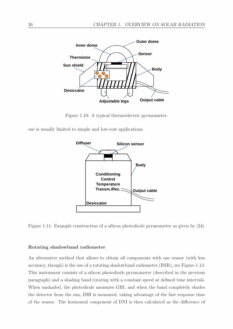
26 CHAPTER 1. OVERVIEW ON SOLAR RADIATION
Inner domeOuter dome
Output cableAdjustable legs
Desiccator
BodySun shield
SensorThermistor
Figure 1.10: A typical thermoelectric pyranometer.
use is usually limited to simple and low-cost applications.
Body
Output cable
Desiccator
Silicon sensor
ConditioningControl
TemperatureTransm./Rec.
Diffuser
Figure 1.11: Example construction of a silicon photodiode pyranometer as given by [24].
Rotating shadowband radiometer
An alternative method that allows to obtain all components with one sensor (with less
accuracy, though) is the use of a rotating shadowband radiometer (RSR), see Figure 1.13.
This instrument consists of a silicon photodiode pyranometer (described in the previous
paragraph) and a shading band rotating with a constant speed at defined time intervals.
When unshaded, the photodiode measures GHI, and when the band completely shades
the detector from the sun, DHI is measured, taking advantage of the fast response time
of the sensor. The horizontal component of DNI is then calculated as the difference of

1.3. GROUND MEASUREMENTS OF SOLAR RADIATION 27
Figure 1.12: Spectral response of silicon (black line) and thermopile (blue) pyranometers,
compared to the solar spectrum at ground level (red) [26].
these two measurements and DNI is obtained by dividing the horizontal beam radiation
by the cosine of the zenith angle at that moment (cf. Equation 1.11). This measurement
includes many uncertainties, such as the temperature dependency of the photodiode, its
spectral response, etc. Nevertheless, it is a less expensive method to obtain DNI and DHI
without using a tracker.
1.3.2 Radiometer calibration
Calibrating an instrument is determining a relation between its input and output val-
ues. Pyranometers and pyrheliometers are calibrated in W/m2 and their sensitivity is in
general in the region 5–20 μVW−1m2. The World Radiometric Reference is the inter-
nationally accepted traceable reference for all radiometer measurements. It is used as a
standard for calibrating solar radiometers and to ensure homogeneity of solar radiation
measurements around the world. The WRR is produced by a group of absolute cavity
radiometers, the World Standard Group (WSG), maintained and operated at the World
Radiation Center (WRC) by the Physical Meteorological Observatory, Davos (PMOD),
in Switzerland [22]. Every five years, an International Pyrheliometer Comparison (IPC)
is held at the PMOD/WRC to transfer the WRR to the participating reference ACR in-
struments, using the sun as the source. The transfer of WRR from the WSG is described
in [27].
Reference pyrheliometers are calibrated by direct comparison with absolute cavity
radiometers traceable to the WRR. The calibration is similar to the transfer of the WRR

28 CHAPTER 1. OVERVIEW ON SOLAR RADIATION
Sensor
Rotating shadow band Motor facing
south
Figure 1.13: Rotating Shadowband Radiometer installed at QEERI’s site.
to the ACR radiometers [28]. The average sensitivity, ratio of the voltage signal of the
test pyrheliometer to the ACR beam irradiance (in units of μVW−1m2), is calculated for
a large range of irradiance levels and solar geometries.
Reference pyranometers are calibrated against a reference ACR by using Equation
1.11 [29] and the ‘sun and shade’ method described in [30], where the pyranometer is first
exposed to the full hemispherical radiation to generate an output voltage Vg and then it is
shaded, so it responds only to the diffuse sky radiation, and generates the output voltage
Vd. The sensitivity can then be calculated from the direct beam radiation measured by
the ACR:
Sensitivity =Vg − Vd
DNI · cos(θz) (1.12)
The calibration methodology of field instruments is performed in laboratories, in com-
parison with a reference instrument of the same type and using artificial sources of light.
The calibration method is described in [31] for field pyranometers and in [32] for field
pyrheliometers.

1.3. GROUND MEASUREMENTS OF SOLAR RADIATION 29
1.3.3 Radiometer properties and classifications
Radiometer measurement errors and uncertainty depend on several factors and properties
characteristic of the radiometer in use. These properties define the relationship of input
values (radiation intensity) to output values (induced voltage), and the most important
are the following:
• Non-linearity of response is the change in sensitivity related to the level of the
incident radiation. It is evaluated as the percentage deviation from the responsivity
at 500 W/m2 due to any change of irradiance within the range 100 to 1100 W/m2.
This effect is mainly attributed to convective and radiative heat losses at the black-
painted surface.
• Temperature response is the change in the sensitivity due to any change in
ambient temperature. The manufacturer provides in general a temperature response
curve for the specific model of the radiometer.
• Zero offsets are the result of the measuring principle of the radiometer. The
radiometer temperature varies in proportion to the ambient temperature and causes
thermal currents inside the instrument, called ‘zero offset type B’. It is quantified in
ISO 9060:1990 as the response inW/m2 to a 5K/hr change in ambient temperature.
The ‘zero offset type A’ only affects pyranometers and is described in Section 1.3.1.
• Response time is the time required by the radiometer to respond to changes in the
incident radiation. In general, it is the time for the output to reach 95% (sometimes
1− 1/e, 63%) of the final value after a step-change in the irradiance.
• Non-stability is the sensitivity drift with time, quoted as the percentage change
of sensitivity over a period of one year of operation of the instrument. This effect
is mostly due to degradation by UV radiation of the black absorber coating on the
thermopile surface. Most manufacturers recommend recalibration every two years.
• Directional response (for pyranometers) is the relative deviation of the measured
value from the ideal value, relative to the angle of incidence of the solar radiation.
Ideally, a sensor should report an intensity value proportional to the cosine of the
zenith angle of the incident radiation, called the ‘cosine response’.
• Spectral selectivity is the variation of the dome transmittance and absorption
coefficient of the black detector coating with wavelength, and is commonly specified
as % of the mean value.
• Tilt response (for pyranometers) is the percentage deviation from the responsivity
at 0 degrees tilt (horizontal) due to changes in tilt from 0 degrees to 90 degrees at
1000 W/m2.

30 CHAPTER 1. OVERVIEW ON SOLAR RADIATION
• Resolution is the smallest change in the amount of radiation that the instrument
can detect.
Classifications and specifications for solar irradiance measurement devices have been
established by ISO 9060/1990 [33] and WMO [22], based on the characteristics listed
above and on the estimated measurement uncertainty of each instrument and their quality.
Tables 1.1 and 1.2 list the WMO characteristics for pyrheliometers and pyranometers,
respectively. Tables 1.3 and 1.4 list the ISO specifications for these radiometers. From
the highest quality to the lowest, three classes are distinguished: secondary standard,
first class and second class. Various models of instruments are available in the market.
These specifications and classifications should be examined in detail in order to get the
required quality of instruments for a particular application.
Characteristic High quality Good quality
Response time < 15 s < 30 s
Zero offset 2 W/m2 4 W/m2
Resolution 0.051 W/m2 1 W/m2
Stability 0.01% 0.05%
Temperature response 1% 2%
Non-linearity 0.02% 0.05%
Spectral sensitivity 0.05% 1.0%
Tilt response 0.02% 0.05%
Achievable uncertainty, 95% conf. level
1-min totals
Percent 0.9 1.8
kJ/m2 0.56 1
Wh/m2 0.16 0.28
1-h totals
Percent 0.7 1.5
kJ/m2 21 54
Wh/m2 5.83 15
Table 1.1: WMO characteristics of operational pyrheliometers for DNI measurements
[22].

1.3. GROUND MEASUREMENTS OF SOLAR RADIATION 31
Characteristic High quality Good quality Moderate quality
Response time < 15 s < 30 s < 60 s
Zero offset
Response to 200 W/m2 net
thermal radiation (ventilated) 7 W/m2 7 W/m2 7 W/m2
Response to 5 K/h change
in ambient temperature 2 W/m2 2 W/m2 2 W/m2
Resolution 1 W/m2 5 W/m2 10 W/m2
Stability 0.08% 1.5% 3%
Directional response 10 W/m2 20 W/m2 30 W/m2
Temperature response 2% 4% 8%
Non-linearity 0.05% 1% 3%
Spectral sensitivity 2% 5% 10%
Tilt response 0.5% 2% 5%
Achievable uncertainty, 95% C.L.
Hourly totals 3% 8% 20%
Daily totals 2% 5% 10%
Table 1.2: WMO characteristics of operational pyranometers for GHI and DHI measure-
ments [22].
Class of pyrheliometerSpecification
Secondary standard First class Second class
Response time < 15 s < 20 s < 30 s
Zero offset ±2 W/m2 ±4 W/m2 ±8 W/m2
Resolution ±0.5 W/m2 ±1 W/m2 ±5 W/m2
Stability ±0.5% ±1% ±2%
Non-linearity ±0.2% ±0.5% ±2%
Spectral selectivity ±0.5% ±1% ±5%
Temperature response ±1% ±2% ±10%
Tilt response ±0.2% ±0.5% ±2%
Traceability With a primary With a secondary With a first class
std. pyrheliometer std. pyrheliometer pyrheliom. or better
Table 1.3: ISO specifications for pyrheliometers used for DNI measurements [33].

32 CHAPTER 1. OVERVIEW ON SOLAR RADIATION
Class of pyranometerSpecification
Secondary standard First class Second class
Response time < 15 s < 30 s < 60 s
Zero offset
Response to 200 W/m2 net
thermal radiation (ventilated) ±7 W/m2 ±15 W/m2 ±30 W/m2
Response to 5 K/h change
in ambient temperature) ±2 W/m2 ±4 W/m2 ±8 W/m2
Resolution ±1 W/m2 ±5 W/m2 ±10 W/m2
Stability ±0.8% ±1.6% ±2%
Non-linearity ±0.2% ±0.5% ±2%
Directional response ±10 W/m2 ±20 W/m2 ±30 W/m2
Spectral selectivity ±2% ±5% ±10%
Temperature response ±2% ±4% ±8%
Tilt response ±0.5% ±2% ±5%
Table 1.4: ISO specifications for pyranometers used for GHI and DHI measurements [33].
1.3.4 Solar radiation monitoring station
Reliable data of solar radiation is key for any solar energy-based project. Direct ground
measurements of solar radiation are the most accurate method for knowing the amount
of incoming solar radiation at a certain location. For this purpose, installing a solar mon-
itoring station to measure the different components of solar radiation simultaneously in a
unique system is fundamental. This system consists of a set of solar sensors mounted on
an automatic two-axis sun tracker which provides a stable platform where all sensors are
placed in optimum positions and, most importantly, moves horizontally in the azimuth
direction and vertically in the zenith direction, following the path of the solar disc, in a
way to continuously point to the sun from sunrise to sunset. This offers an uninterrupted
measurement of solar radiation through the following sensors (described above): one
pyrheliometer for direct normal irradiance, one pyranometer for global horizontal irradi-
ance and another pyranometer for diffuse horizontal irradiance with a shading assembly
mounted in a way to shade the dome of the pyranometer and block the direct radiation.
A solar station can also host a pyrgeometer (for far infrared long-wave radiation), UV
radiometer, albedometer or other sensors.
A number of considerations should be taken into account before installing a solar
monitoring station:
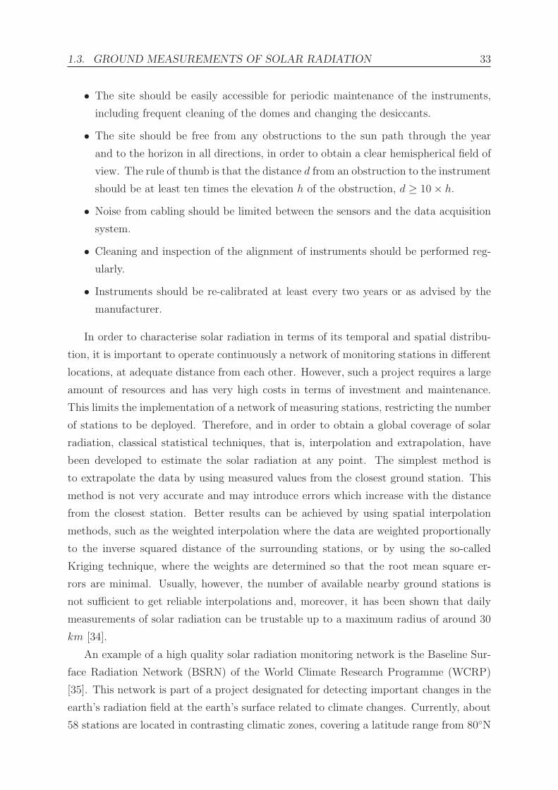
1.3. GROUND MEASUREMENTS OF SOLAR RADIATION 33
• The site should be easily accessible for periodic maintenance of the instruments,
including frequent cleaning of the domes and changing the desiccants.
• The site should be free from any obstructions to the sun path through the year
and to the horizon in all directions, in order to obtain a clear hemispherical field of
view. The rule of thumb is that the distance d from an obstruction to the instrument
should be at least ten times the elevation h of the obstruction, d ≥ 10× h.
• Noise from cabling should be limited between the sensors and the data acquisition
system.
• Cleaning and inspection of the alignment of instruments should be performed reg-
ularly.
• Instruments should be re-calibrated at least every two years or as advised by the
manufacturer.
In order to characterise solar radiation in terms of its temporal and spatial distribu-
tion, it is important to operate continuously a network of monitoring stations in different
locations, at adequate distance from each other. However, such a project requires a large
amount of resources and has very high costs in terms of investment and maintenance.
This limits the implementation of a network of measuring stations, restricting the number
of stations to be deployed. Therefore, and in order to obtain a global coverage of solar
radiation, classical statistical techniques, that is, interpolation and extrapolation, have
been developed to estimate the solar radiation at any point. The simplest method is
to extrapolate the data by using measured values from the closest ground station. This
method is not very accurate and may introduce errors which increase with the distance
from the closest station. Better results can be achieved by using spatial interpolation
methods, such as the weighted interpolation where the data are weighted proportionally
to the inverse squared distance of the surrounding stations, or by using the so-called
Kriging technique, where the weights are determined so that the root mean square er-
rors are minimal. Usually, however, the number of available nearby ground stations is
not sufficient to get reliable interpolations and, moreover, it has been shown that daily
measurements of solar radiation can be trustable up to a maximum radius of around 30
km [34].
An example of a high quality solar radiation monitoring network is the Baseline Sur-
face Radiation Network (BSRN) of the World Climate Research Programme (WCRP)
[35]. This network is part of a project designated for detecting important changes in the
earth’s radiation field at the earth’s surface related to climate changes. Currently, about
58 stations are located in contrasting climatic zones, covering a latitude range from 80◦N
34 CHAPTER 1. OVERVIEW ON SOLAR RADIATION
to 90◦S. The World Radiation Data Centre (WRDC) of the WMO [36], on the other hand,
is an online database maintained by the Russian Federal Service for Hydrometeorology
and Environmental Monitoring, and serves as a central depository for solar radiation data
collected at over one thousand measurement sites throughout the world. In Qatar, the
Qatar Meteorological Department (QMD) currently operates a network of 12 automated
weather stations (AWS) distributed in coastal and inland locations throughout the coun-
try, and most of these stations have been collecting global horizontal irradiation data
from as early as 2007, along with meteorological parameters. For more details on the
QMD network, see Section 5.1.
1.4 Solar radiation modelling
Although ground measurements of solar radiation, if the used instrumentation is well
maintained and regularly calibrated, represent the most accurate option for the knowledge
of solar radiation data, they are not always available, and solar radiation monitoring
networks have limited coverage. In the absence of ground measurements, models have
been developed for the estimation of solar radiation. These models can be based on
empirical approaches, using meteorological parameters or atmospheric constituents or
a more readily available solar radiation component. They can also be quasi-physical
and physical, considering the radiative extinction processes in the atmosphere. Artificial
Neural Network models have also been developed for solar radiation estimation.
1.4.1 Empirical models
Empirical methods use a relationship between the atmospheric transmissivity and other
meteorological parameters and are mostly based on measured radiation data at specific
sites. Meteorological parameters used to model solar radiation may include sunshine
duration, temperature, cloud cover, precipitation and humidity. The accuracy of the
model depends on the used parameters and the way they are implemented in the model.
The first empirical model for estimating global solar radiation was developed by
Angstrom and is based on the hours of sunshine duration, using data generally avail-
able in many locations [37]. Several regression models, based on the Angstrom model,
have been proposed, with a resulting linear equation given by:
H
H0
= a+ bS
S0
, (1.13)
where H and H0 are, respectively, the monthly averages of daily global radiation and
1.4. SOLAR RADIATION MODELLING 35
of daily extraterrestrial radiation on the horizontal surface, S and S0 are the monthly
averages of daily hours of bright sunshine and of maximum possible daily sunshine hours
(the day length), a and b are empirical constants depending on the location.
It was found that this linear-type equation cannot be applicable for particular days
with extreme values, leading to overestimation of the total radiation on cloudless days
when SS0
= 1 and on overcast days when SS0
= 0. A quadratic form was then suggested
for the relationship between the ratio of daily global to extraterrestrial radiation and
actual to maximum possible hours of sunshine greater than zero. Others suggest multi-
linear regression equations with combinations of one or more weather parameters such as
temperature, relative humidity, and relative sunshine duration [38]. The Angstrom-type
empirical models were reviewed by Gueymard et al. in [39], covering the errors coming
from instrumental measurements of S and the effects of seasonal and climate variability.
Another empirical method which has been extensively used is the air temperature-
based model [40], since air temperature measurements are available at many locations
from the majority of meteorological stations. The method is based on the calculation
of the difference between the maximum and minimum temperatures, which has different
range on clear days than on overcast or rainy days.
Of particular interest to this work is the direct normal irradiance. Many empirical
models have been developed to derive DNI by statistical means from other, more readily
available data. One approach is to use the global solar radiation in order to estimate
the direct component, through an empirical relationship between the global and direct
clearness indices or transmittances, Kt and Kn [41]. The global clearness index Kt is
defined as the ratio of global horizontal radiation at the earth’s surface (GHI) to the
global horizontal radiation at the top of the atmosphere. The direct clearness index Kn
is the same ratio but for the beam (direct) components. Another empirical approach
for direct normal radiation estimation is to correlate the diffuse ratio to Kt. The diffuse
ratio is the fraction of the radiation on a horizontal plane which is diffuse, i.e., the ratio
DHI/GHI. Many well-known models have been proposed based on this correlation. To
cite, Orgill and Hollands in 1977 [42], Erbs in 1982 [43] and Reindl et al. in 1999 [44].
Each of these models is derived from a different data set of ground measurements. In
general, all the cited models are almost identical and give similar results for practical
purposes. Below is the equation of the diffuse fraction as given by the Erbs correlation

36 CHAPTER 1. OVERVIEW ON SOLAR RADIATION
for hourly radiation and clearness index:
DHI
GHI=
⎧⎪⎪⎪⎨⎪⎪⎪⎩1− 0.09Kt, if Kt ≤ 0.22
0.9511− 0.1604Kt + 4.388K2t − 16.638K3
t + 12.336K4t , for 0.22 < Kt ≤ 0.08
0.165, for Kt > 0.8
(1.14)
The main limitation of any empirical-based solar radiation model is that it is site-
dependent. However, in most of the cases the overall equation of any of these models can
be applied with revised coefficients and constants depending on the particular location.
1.4.2 Quasi-physical and physical models
The Direct Insolation Simulation Code (DISC) is a quasi-physical model developed by
E. Maxwell [45]. It makes use of the global horizontal irradiance measurements, but also
needs the sun zenith angle, day of the year, and the site’s average atmospheric pressure as
inputs for the estimation of the direct radiation. The algorithm uses physical principles
for the improvement of the empirical relationship between the global and direct clearness
indices. The DirInt model developed by Richard Perez is an improved version of the DISC
model, based on binning the zenith angle, the global clearness index Kt, and dew point
temperature in a way to have an indication of the sky condition. This method results
in finding a coefficient from a four-dimensional look-up table to be used to improve the
estimation of DNI by the DISC model. In the DirIndex model, the same approach as
in DirInt is used but taking into account the atmospheric turbidity, which has a high
influence on the beam irradiance [46].
Physical models are based on codes which model the transfer of solar radiation through
the atmosphere. As mentioned before, solar radiation traversing the atmosphere is ab-
sorbed and scattered by the atmospheric constituents, which are highly variable in space
and time. This makes it very complex to model the radiative transfer and requires various
input parameters, each of them describing the atmospheric extinction sources in the path
of the direct beam. The spectral distribution of the extraterrestrial direct beam radiation
and the modification of its spectrum due to the wavelength dependence of the scattering
and absorption processes, lead to a complex calculation of DNI. Spectral models span
from the very complex ‘line-by-line’ models to the less complex spectral band models
such as MODTRAN, and are mostly used in atmospheric sciences.
In most solar applications, physical models are based on the calculation of the phys-
ical extinction of radiation through the atmosphere by means of a broadband approach
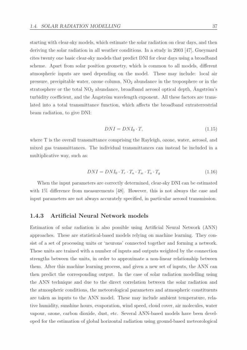
1.4. SOLAR RADIATION MODELLING 37
starting with clear-sky models, which estimate the solar radiation on clear days, and then
deriving the solar radiation in all weather conditions. In a study in 2003 [47], Gueymard
cites twenty one basic clear-sky models that predict DNI for clear days using a broadband
scheme. Apart from solar position geometry, which is common to all models, different
atmospheric inputs are used depending on the model. These may include: local air
pressure, precipitable water, ozone column, NO2 abundance in the troposphere or in the
stratosphere or the total NO2 abundance, broadband aerosol optical depth, Angstrom’s
turbidity coefficient, and the Angstrom wavelength exponent. All these factors are trans-
lated into a total transmittance function, which affects the broadband extraterrestrial
beam radiation, to give DNI:
DNI = DNI0 · T, (1.15)
where T is the overall transmittance comprising the Rayleigh, ozone, water, aerosol, and
mixed gas transmittances. The individual transmittances can instead be included in a
multiplicative way, such as:
DNI = DNI0 · Tr · Ta · Tw · To · Tg (1.16)
When the input parameters are correctly determined, clear-sky DNI can be estimated
with 1% difference from measurements [48]. However, this is not always the case and
input parameters are not always accurately specified, in particular aerosol transmission.
1.4.3 Artificial Neural Network models
Estimation of solar radiation is also possible using Artificial Neural Network (ANN)
approaches. These are statistical-based models relying on machine learning. They con-
sist of a set of processing units or ‘neurons’ connected together and forming a network.
These units are trained with a number of inputs and outputs weighted by the connection
strengths between the units, in order to approximate a non-linear relationship between
them. After this machine learning process, and given a new set of inputs, the ANN can
then predict the corresponding output. In the case of solar radiation modelling using
the ANN technique and due to the direct correlation between the solar radiation and
the atmospheric conditions, the meteorological parameters and atmospheric constituents
are taken as inputs to the ANN model. These may include ambient temperature, rela-
tive humidity, sunshine hours, evaporation, wind speed, cloud cover, air molecules, water
vapour, ozone, carbon dioxide, dust, etc. Several ANN-based models have been devel-
oped for the estimation of global horizontal radiation using ground-based meteorological

38 CHAPTER 1. OVERVIEW ON SOLAR RADIATION
measurements as inputs [49, 50]. Satellite observations can also be used as ANN inputs
for the estimation of the global [51] or the direct [52] solar radiation.
1.5 Satellite-derived solar data
Methods based on satellite observations represent an alternative for the estimation of so-
lar radiation and are widely used [53, 54, 55]. Solar energy-based projects commonly use
long-term satellite data in combination with high-quality short-term solar ground mea-
surements for solar resource assessment purposes. According to Zelenka et al. [56], hourly
irradiation data derived from satellites are considered the most accurate option for solar
radiation prediction in locations at distances greater than 25 km from a ground station.
Meteorological satellites scan the earth’s surface, and based on the produced images it is
possible to retrieve the solar radiation components at ground level with relatively high
spatial and temporal resolution. For instance, the satellites of the Meteosat Second Gen-
eration (MSG) provide images of Europe, Africa and the North Atlantic since 2004, with a
temporal resolution of 15 minutes and spatial resolution of approximately 1 km×1 km at
sub-satellite point. Imagers on-board the satellite observe the earth in different spectral
channels and provide information and data of the state of the atmosphere.
Several methods exist for deriving solar radiation from satellite observations. They
can be divided into empirical or physical methods. The empirical methods consist of es-
tablishing relationships between satellite- and ground-based observations to give an (em-
pirical) estimation of solar radiation. Physical methods use satellite information directly
to determine the atmospheric properties, for the estimation of the surface solar radiation.
Improvements in many aspects of the modelling processes have led to the derivation of
solar radiation from satellite images using both empirical and physical information in a
hybrid approach [57].
There are two types of meteorological satellites:
• Polar-orbiting weather satellites, thus called because by circling the earth they
pass over the poles. They are located at low altitudes, around 850 km above the
ground, offering higher resolution information. With the polar satellites, every
location on earth can be observed twice each day. This low temporal resolution
limits their operational use for the estimation of surface solar radiation. Several
countries operate polar-orbiting meteorological satellites, such as NOAA by the
United States and the European Metop-A and Metop-B satellites. Russia has the
Meteor and Resurs series of satellites. Recently, the Advanced Very High Resolution
Radiometer (AVHRR), on board the polar-orbiting NOAA and Metop satellites,

1.5. SATELLITE-DERIVED SOLAR DATA 39
provides information several times a day, which allows the solar radiation estimation
with higher confidence, as studied by Karlsson et al. in [58].
• Geostationary weather satellites are suspended at the same place above the equator
at an altitude of about 36000 km. Since they orbit the earth in the same direction
and speed as the earth’s rotation, they remain stationary as viewed from the earth’s
surface and thus provide continuous information of the entire hemisphere seen by
the satellite. Several geostationary meteorological satellites are in operation cover-
ing the whole world except the poles and include the United States Geostationary
Operational Environmental System (GOES), the European Meteosat Missions, the
Indian INSAT, the Japanese MTSAT, the Russian new-generation weather satellite
Elektro-L1, and the Chinese Feng-Yun geostationary satellites. In general, geosta-
tionary satellites are the most used for the derivation of solar radiation data due to
the high temporal resolution that they can offer.
The basis of satellite-based methods is the equation of energy conservation, taking
into account the interaction of the extraterrestrial radiation with the atmospheric con-
stituents before reaching the earth’s surface. When the solar radiation traverses the
atmosphere, it is partly reflected back to space and partly absorbed by the atmosphere.
The remaining part which reaches the ground is partly absorbed by the earth’s surface
and partly reflected back (affected again by atmospheric diffusion and absorption) to
space as the surface albedo. The satellite sensor measures the radiation backscattered by
the earth-atmosphere system. Following this energy conservation scheme and by knowing
the absorbed energy and the surface albedo, the solar radiation on the earth’s surface can
be derived. The extraterrestrial radiation is retrieved by astronomical equations and the
reflected radiation is measured by the satellite radiometers. For more details on the ex-
pression of energy conservation for the derivation of solar radiation at the earth’s surface,
see [59].
In the following, one renowned method, Heliosat, is briefly described in order to give
an overview on the derivation of solar radiation from satellite observations. Heliosat is
developed and continuously improved by the Centre for Energy and Processes, Ecole des
Mines de Paris/Armines, France. Originally, the model was developed by Cano et al.
[53], and has been followed by different versions for model improvement. The original
concept consists of statistically determining the global solar irradiance from the amount
of cloud cover over a given area and time. This includes the derivation of a cloud cover
index n for each pixel of the original satellite image, as follows:
n =ρ− ρgρc − ρg
, (1.17)

40 CHAPTER 1. OVERVIEW ON SOLAR RADIATION
where ρ is the albedo measured by the satellite, ρc is the cloud albedo of a heavily overcast
sky, and ρg is the ground albedo, associated to a clear, clean and dry sky. The cloud
cover index ranges from 0 to 1.
The first version, Heliosat-1, as defined by Diabate et al. [60], considers a linear
correlation between the cloud cover index n and the instantaneous clearness index Kt:
Kt = an+ b, (1.18)
where a and b are empirical parameters. Heliosat-1 uses numerical counts of the satellite
images for the calculation of the albedos, so that ρ is measured by the digital counts of
the sensor, ρc represents the maximum count, and ρg represents the minimum count. The
Heliosat-2 version uses calibrated radiances instead of the digital counts and considers
atmospheric extinction and cloud extinction separately. The clear-sky solar irradiance is
derived from the European Solar Radiation Atlas (ESRA) model [61], taking the Linke
turbidity as input parameter; the Linke turbidity factor being the number of clear and
dry atmospheres needed to give the optical thickness of the atmosphere due to both the
absorption by the water vapour and absorption and scattering by the aerosol particles.
The Heliosat-3 version is based on a radiative transfer code, the SOLIS model scheme.
It uses as inputs the atmospheric parameters information (clouds, ozone, and water
vapour, and aerosols) derived from the Second Generation of the Meteosat satellite
databases MSG or other platforms.
Heliosat-4 is the newest version of the Heliosat method, created by MINES ParisTech
and the German Aerospace Centre DLR (Deutsches Zentrum fur Luft- und Raumfahrt).
It is based on a fully physical model using an approximation of the libRadtran radiative
transfer model. It is composed of the McClear model for clear-sky irradiances and the
McCloud model for calculating the extinction of irradiance due to clouds. Inputs to
Heliosat-4 are atmospheric products derived from the MACC database, ground albedo
derived from the MODIS data, and cloud properties derived from images of the Meteosat
satellites. For more information on the Heliosat-4 method, see [62].
Direct and diffuse irradiances are in general derived from the satellite-derived global
irradiance by using the separation or decomposition models as discussed in Section 1.4.1.
However, there are other methods to derive the direct normal irradiance directly from
the satellite images. These methods are usually based on a clear sky model where DNI
under clear-sky conditions follows Equation 1.16. DNI for cloudy conditions is estimated
by multiplying DNIclear by a transmission coefficient of clouds. The transmittances
for the attenuation by gases, ozone, water vapour and aerosols, are determined from
different meteorological satellites or other sources. The transmission coefficient of clouds

1.6. SOLAR RADIATION AS RENEWABLE SOURCE OF ENERGY 41
is function of a cloud index derived from the infrared (IR) and visible (VIS) channels
of the Meteosat satellite images, see for instance the Solar Energy Mining (SOLEMI)
method of DLR [63].
In all cases, the estimation of solar radiation from satellite images should be validated
and calibrated with high-quality ground data covering different time periods and ground
areas. Statistical parameters like MBE (mean bias error) and RMSE (root mean square
error) are used to quantify the accuracy of the assessment of the satellite models. In [59],
a table summarising the results of the accuracy of the satellite models in terms of MBE
and RMSE from several studies, shows that the RMSE of the global hourly radiation lies
between 17–25%, and between 10–15% for the daily estimations. Larger errors are found
for DNI, due to the high dynamicity of this component. Task 36 of Solar Heating and
Cooling – International Energy Agency [64] proposes a standardisation of procedures for
benchmarking and ways to improve the quality of satellite estimations. Several web-based
services and databases offering solar radiation information from satellite observations are
currently available, either from commercial providers [65, 66, 67, 68, 69], or for free
[70, 71]. For more details on different satellite models available, see the NREL Best
Practices Handbook [72].
1.6 Solar radiation as renewable source of energy
The clean and plentiful resource of solar energy can be gathered with solar collectors and
converted into another form of energy such as heat or electricity. This can be possible
through passive solar techniques and measures to trap and store the solar radiation, such
as effective spaces design, building orientation towards the sun and selection of materials
with good thermal properties, but also through active solar techniques using solar energy
conversion systems. Solar photovoltaic (PV) and concentrating photovoltaics (CPV)
directly convert solar energy into electricity, while Concentrating Solar Power (CSP)
systems convert the solar energy into heat, then the heat is transformed into electricity.
The conversion of solar energy to electricity by using PV devices is based on the
photoelectric effect: the direct creation of an electric current in a semiconductor material
upon exposure to light. The smallest unit of a PV system is a cell. Cells are wired
together to produce PV modules, and modules are assembled together to form a panel.
A group of panels creates an array, and a group of arrays forms the array field of a PV
facility. The chain is illustrated in Figure 1.14.
PV cells are made of thin layers of positive- and negative-type semiconductors, forming
a p-n junction and creating an electric field. A typical silicon PV cell is composed of an
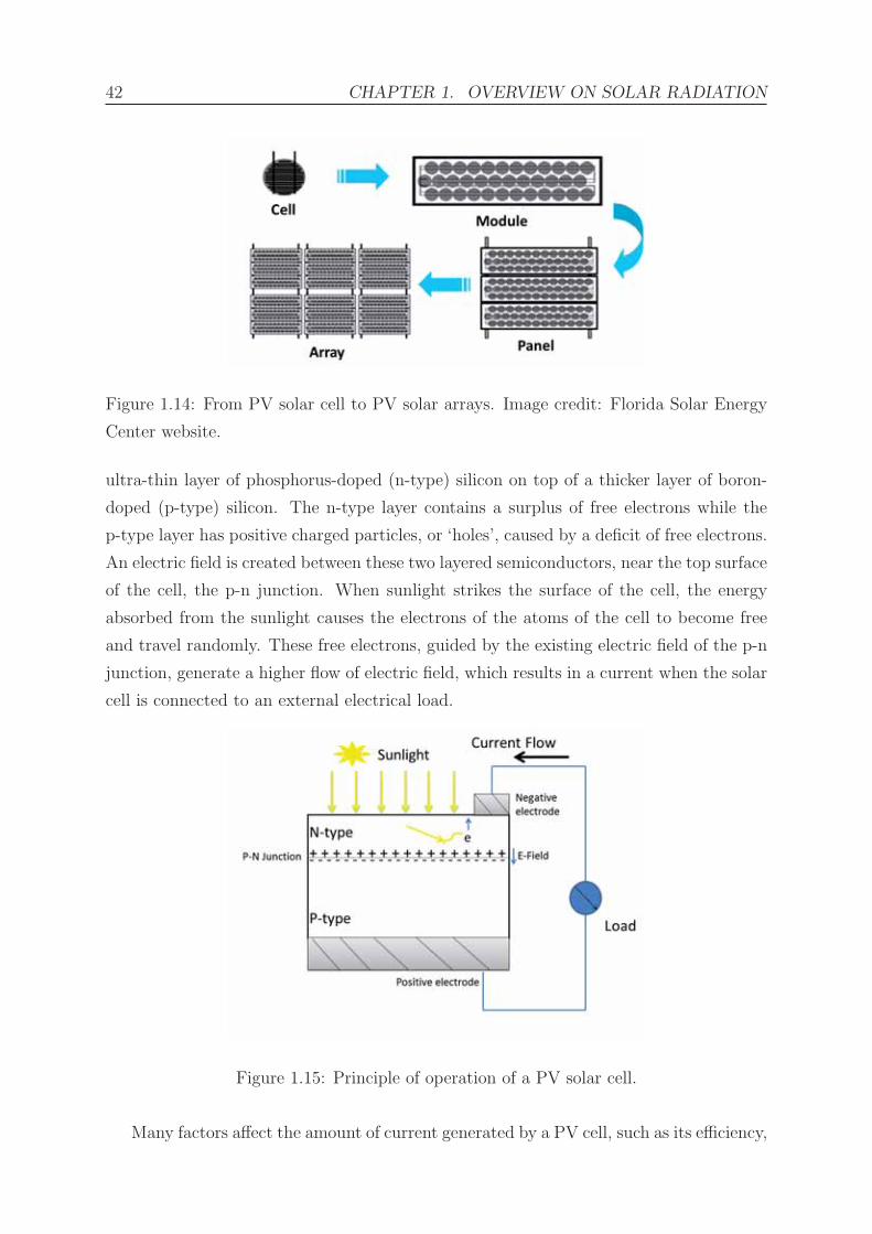
42 CHAPTER 1. OVERVIEW ON SOLAR RADIATION
Figure 1.14: From PV solar cell to PV solar arrays. Image credit: Florida Solar Energy
Center website.
ultra-thin layer of phosphorus-doped (n-type) silicon on top of a thicker layer of boron-
doped (p-type) silicon. The n-type layer contains a surplus of free electrons while the
p-type layer has positive charged particles, or ‘holes’, caused by a deficit of free electrons.
An electric field is created between these two layered semiconductors, near the top surface
of the cell, the p-n junction. When sunlight strikes the surface of the cell, the energy
absorbed from the sunlight causes the electrons of the atoms of the cell to become free
and travel randomly. These free electrons, guided by the existing electric field of the p-n
junction, generate a higher flow of electric field, which results in a current when the solar
cell is connected to an external electrical load.
Figure 1.15: Principle of operation of a PV solar cell.
Many factors affect the amount of current generated by a PV cell, such as its efficiency,

1.6. SOLAR RADIATION AS RENEWABLE SOURCE OF ENERGY 43
its size and the intensity of the incident solar radiation. The most common type of
materials used for PV cells are semi-conductor crystalline silicon and quartz. Other
materials, manufactured in thin films and incorporated into modules, include amorphous
silicon, cadmium telluride or copper indium di-selenide. Typically, silicon modules have
efficiencies of ∼ 12–16%, while thin-film modules have efficiencies of ∼ 9–13%, depending
on the technology [73].
Similarly to the conventional PV systems, CPV also uses the photovoltaic effect to
directly convert sunlight into electricity, except that they make use of lenses and mirrors
to concentrate the direct solar radiation onto a smaller area of multi-junction solar cells,
thus increasing the efficiency level to about 40%. CPV uses solar trackers to automatically
follow the sun. For more information on CPV systems, see [74].
Solar thermal collectors, on the other hand, receive the solar radiation from the sun
and convert it into heat which can be used for many purposes such as water heating,
space heating and cooling, and heating fluids to high temperature. The solar collectors
can be either concentrating or non-concentrating.
The most common type of non-concentrating collectors are flat-plate collectors and
operate at low and medium temperatures. They are usually employed for swimming pool
heating or heating water or air for residential and commercial use. A common design of a
flat-plate collector is illustrated in Figure 1.16 and consists of an absorber that intercepts
and absorbs the solar energy, a transparent cover to reduce heat loss from the absorber,
and a heat-transfer fluid (air or water) circulating through tubes to transfer the heat
from the absorber to a heat-insulating backing.
Figure 1.16: A liquid flat-plate collector [75].
Concentrating collectors are high-temperature collectors which concentrate sunlight
using mirrors or lenses. They are generally used to heat a fluid to produce steam and
operate a turbine for electricity generation in solar thermal power plants. The heat is
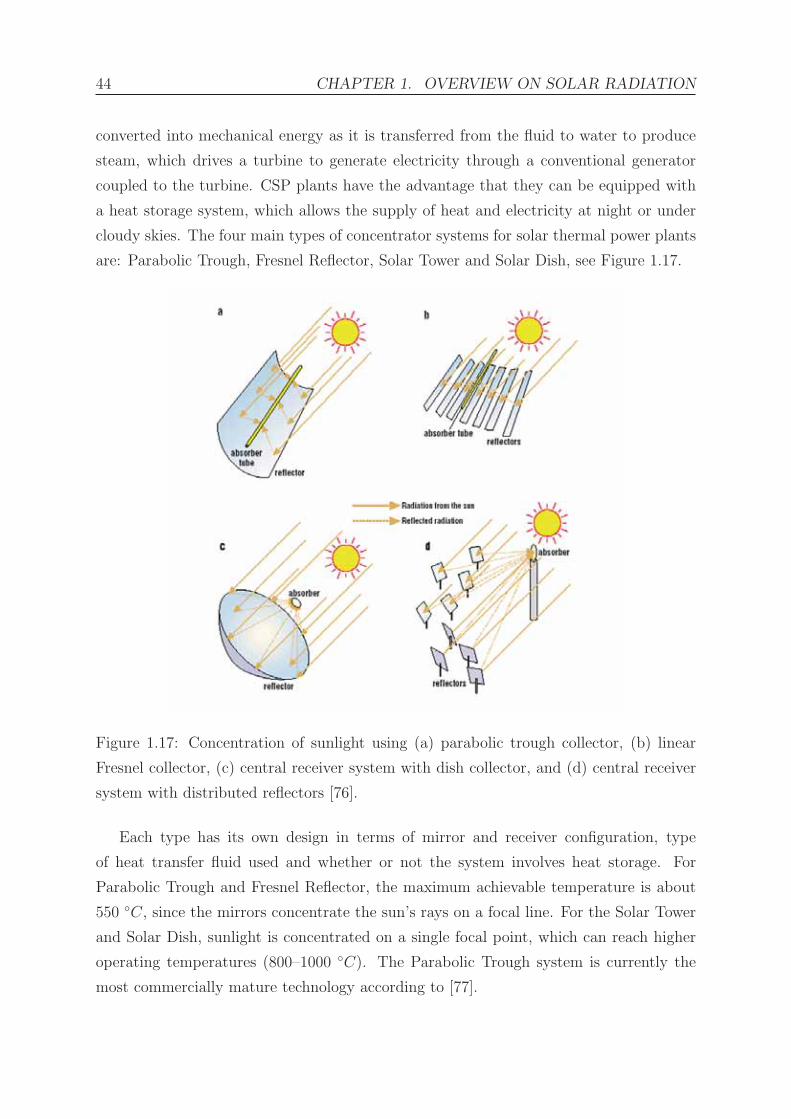
44 CHAPTER 1. OVERVIEW ON SOLAR RADIATION
converted into mechanical energy as it is transferred from the fluid to water to produce
steam, which drives a turbine to generate electricity through a conventional generator
coupled to the turbine. CSP plants have the advantage that they can be equipped with
a heat storage system, which allows the supply of heat and electricity at night or under
cloudy skies. The four main types of concentrator systems for solar thermal power plants
are: Parabolic Trough, Fresnel Reflector, Solar Tower and Solar Dish, see Figure 1.17.
Figure 1.17: Concentration of sunlight using (a) parabolic trough collector, (b) linear
Fresnel collector, (c) central receiver system with dish collector, and (d) central receiver
system with distributed reflectors [76].
Each type has its own design in terms of mirror and receiver configuration, type
of heat transfer fluid used and whether or not the system involves heat storage. For
Parabolic Trough and Fresnel Reflector, the maximum achievable temperature is about
550 ◦C, since the mirrors concentrate the sun’s rays on a focal line. For the Solar Tower
and Solar Dish, sunlight is concentrated on a single focal point, which can reach higher
operating temperatures (800–1000 ◦C). The Parabolic Trough system is currently the
most commercially mature technology according to [77].

Chapter 2
Atmospheric Properties and Lidar
Techniques
This chapter provides basic information on the atmospheric structure and properties. The
atmospheric boundary layer (ABL), the lowest part of the troposphere, is described in
more detail. Aerosols and their influence on the earth’s radiation budget are discussed.
A short description of the interaction of light with atmospheric constituents is given,
including the theories of scattering of light by molecules and particles: the Rayleigh and
Mie theories. Finally, since lidar has been proven to be an effective tool for profiling the
atmosphere and detecting aerosol layers, this chapter gives also an overview about the
lidar technique, with an expanded description of the elastic backscatter lidar.
2.1 Atmospheric structure
The earth’s atmosphere is a relatively thin layer of gases that surrounds the earth. The
mass of the atmosphere is around 5×10¹⁸ kg, and 99% of this mass is within the first
30 km from the earth’s surface. In the atmosphere, both pressure and density decrease
with height. Temperature has, however, a varying profile; it may decrease, increase or
remain relatively constant with height, dividing the atmosphere into five main layers. The
troposphere is the lowest and major part of the atmosphere, since it contains up to 75%
of the mass of the atmosphere, and most of the atmospheric aerosols and water vapour.
Within it, day-to-day weather phenomena occur and molecules and particulates are well
mixed. This layer extends from the earth’s surface up to about 10 km in mid-latitudes
and to about 15 km at the equator. Within this layer, temperature decreases with height
at a constant rate. The lowest part of the troposphere is the Atmospheric Boundary Layer
(ABL), also called the planetary boundary layer (PBL), or sometimes simply boundary
45

46 CHAPTER 2. ATMOSPHERIC PROPERTIES AND LIDAR TECHNIQUES
layer (BL), where most of the human activities take place. This sublayer will be further
described in Section 2.1.2. The stratosphere starts at around 10–15 km, reaching 50
km above the surface (at mid-latitudes) and containing the ozone layer. It is a stable
and stratified layer where the temperature increases with increasing altitude. This is
due to the absorption of ultraviolet (UV) solar radiation by the ozone layer. Molecules
dominate in this layer; however, in the lower part of the stratosphere, particulates can also
be present mainly from aircraft engine exhaust or volcanic eruptions. In the middle of the
atmosphere, is the mesosphere, where the air is thin and the temperature decreases with
altitude due to little absorption of solar energy at this level. A high concentration of ions
is present at the upper level of this layer. Above the mesosphere lays the thermosphere,
from around 80 km up to 400 km, where a significant temperature inversion is observed.
It is a relatively warm layer because of the presence of oxygen, which absorbs the UV
energy from the sun. The exosphere is the top layer of the atmosphere and the farthest
away from the surface. It extends from approximately 500 km to about 1000 km, but
it doesn’t have clear boundaries, i.e., lower and upper limits. Molecule concentrations
in this layer are small, so they do not collide with each other, and can escape to outer
space. These various atmospheric layers are depicted schematically in Figure 2.1.
Temperature (C)
Alti
tude
(km
)
10
50
100
500Exosphere
Thermosphere
Mesosphere
Stratosphere
Troposphere0 50 100 150-50-100 200
e
Figure 2.1: The major layers within the atmosphere, based on the vertical distribution
and variations of the temperature (red line) in the atmosphere.

2.1. ATMOSPHERIC STRUCTURE 47
2.1.1 Composition of the atmosphere
The composition of the atmosphere can be divided into a ‘clean dry’ component, water
vapour, and aerosols. Table 2.1 lists the major gaseous components of the atmosphere
with their proportions. As shown, the atmosphere is mainly composed of nitrogen (N2,
78% by volume), oxygen (O2, 21% by volume), and argon (Ar, 1% by volume). The
remaining components, although present in small amounts, play an important role in
the earth’s energy balance through the different radiative processes and their efficiency
in trapping the solar radiation. These gases are called greenhouse gases and the most
important are carbon dioxide and ozone. Water vapour is also an important greenhouse
gas; it accounts for roughly 0.25% of the atmospheric mass and its concentration in the
atmosphere is highly variable among different regions. Aerosols account for only a minute
fraction of the mass of the atmosphere. Yet, they have a high influence on the energy
balance of the earth, and affect the hydrological cycle and the abundance of greenhouse
and reactive trace gases.
Molecular Fractional concentra-Constituent
weight [g/mol] tion by volume
Nitrogen (N2) 28.013 78.08%
Oxygen (O2) 32.000 20.95%
Argon (Ar) 39.95 0.93%
Water vapour (H2O)* 18.02 0–5%
Carbon dioxide (CO2)* 44.01 380 ppm
Neon (Ne) 20.18 18 ppm
Helium (He) 4 5 ppm
Methane (CH4)* 16.04 1.75 ppm
Krypton (Kr) 83.80 1 ppm
Hydrogen (H2) 2.02 0.5 ppm
Nitrous oxide (N2O)* 56.03 0.3 ppm
Ozone (O3)* 48 0–0.1 ppm
Table 2.1: Major gaseous constituents of the earth’s atmosphere,
up to an altitude of 105 km, with respect to dry air [78].
* The so-called greenhouse gases.

48 CHAPTER 2. ATMOSPHERIC PROPERTIES AND LIDAR TECHNIQUES
2.1.2 Atmospheric boundary layer
As seen in Section 2.1, the troposphere extends from the ground up to an average of 10 to
15 km. The atmospheric or planetary boundary layer is the lowest part of the troposphere,
where human and other living organisms are present and where almost all of the energy,
water vapour and aerosols are created and transported to the upper atmosphere. Stull
[79] defines the boundary layer as “that part of the atmosphere that is directly influenced
by the presence of the earth’s surface, and responds to surface forcings with a timescale
of about an hour or less”. Kaimal and Finnigan [80] describe this layer as the “lowest 1–2
km of the atmosphere, the region most directly influenced by the exchange of momentum,
heat, and water vapour at the earth’s surface”. The ABL is influenced by the earth’s
surface through several forcings like friction, pollutant emissions and heat and cooling
fluxes on the ground. Depending on the forcing, the ABL depth can range from hundreds
to even several thousand metres from the surface level [81]. Moreover, the depth of the
ABL is influenced by the location, topographical features on the ground, season, time
of the day and weather. The top of the ABL shows a sharp increase in temperature
and drop in the concentration of particulates and water vapour. It is separated from
the ‘free atmosphere’ above it by the capping inversion, a stable layer of warm air above
cool air, that prevents convection and dynamic liftings, trapping pollutants in the ABL.
Being influenced by the solar heating, the ABL height varies during one day and several
sublayers are found within it:
Surface layer is the layer closest to the surface; its height ranges from 50 to 100 m,
about 10% of the ABL height. The surface layer is characterised by large gradi-
ents of atmospheric properties: temperature, moisture, wind speed and trace gas
concentrations.
Convective boundary layer, also called the mixing layer, is the layer where particles
are well mixed due to surface-air interaction in mechanical and thermal forms.
After sunrise, solar heating causes thermals of warm air to rise upwards until their
temperatures drop to the same temperature of the surrounding air.
Residual layer is the layer of particles being left from the previous convective layer
after sunset or from long-range transportation of winds.
The study of the diurnal variation of the ABL plays a crucial role in the determination
of atmospheric pollutants’ dispersion pathways and their chemical properties. At night, a
more stable layer grows and forms the nocturnal boundary layer around sunset, in which
mixing is caused by wind friction. The highest stable nocturnal boundary layer is less

2.1. ATMOSPHERIC STRUCTURE 49
Figure 2.2: Diurnal evolution of the atmospheric boundary layer.
than 400 to 500 m in height, see [82]. Absence of convection during the night creates
vertical stratification. Figure 2.2 shows the typical evolution of the atmospheric boundary
layer. Examples of the formation of these layers and their evolution with time during a
day are given in Figure 4.7, discussed in Chapter 4. The figure shows the formation and
evolution of the boundary layer and other layers in the atmosphere for several days, as
acquired by the Lidar-ceilometer installed at the QEERI facility in Doha, Qatar.
2.1.3 Aerosols in the troposphere
Atmospheric aerosols play an important role in the atmospheric radiative transfer. They
have large influence on climate change and the earth’s radiation budget [83], despite being
only a minor constituent of the atmosphere, as discussed in Section 2.1.1. An aerosol is
defined in its simplest form as a collection of solid or liquid particles suspended in a
gas [84]. Atmospheric aerosols are a complex and dynamic mixture of solid and liquid
particles originating from natural and anthropogenic sources as primary emissions, i.e.,
introduced directly into the atmosphere, or secondary, i.e., formed in the atmosphere
through chemical reactions. This includes a wide range of phenomena such as dust,
fume, smoke, mist, fog, haze and clouds. Aerosols exhibit large diversity in terms of their
properties. Depending on the sources and the meteorological processes, aerosols vary in
shape, chemical composition, lifetime, transformation and removal mechanisms, physical
and optical properties.
Various distributions have been used to fit the aerosol size distribution, such as the

50 CHAPTER 2. ATMOSPHERIC PROPERTIES AND LIDAR TECHNIQUES
power law, the modified gamma and the log-normal distributions [85]. Their sizes can
cover a wide range, from few nanometres to tens of micrometres. Particles of diameter
d < 2.5 μm are considered in the fine mode. Particles of diameter d > 2.5 μm represent
the coarse mode. Fine mode is divided into the nuclei mode (0.005 μm < d < 0.1
μm) and accumulation mode (0.1 μm < d < 2.5 μm). Although this classification is
important, there is no strict scientific classification of aerosols; they can be also classified
based on their physical form and method of generation. In climate models, for instance,
aerosols are subdivided into different types based on the properties of their components.
Components may include soil particles, sulphates and nitrates, soot, sea-salt particles,
desert dust and sulphate droplets. Table 2.2 shows the different types of aerosols along
with their properties which represent average conditions, as detailed in [86]. N is the
number concentration, reff is the effective radius describing the mean size of the particle
ensemble, ssa is the single-scattering albedo defined as the ratio of total scattering to
extinction of the particle, g is the asymmetry parameter, which is a measure of the light
scattered toward the forward direction compared to the light scattered toward the back
direction, and a is the Angstrom exponent describing the spectral slope of the optical
coefficients.
N reff ssa g a aAerosol type
cm−3 μm 0.55 μm 0.55 μm 0.35–0.55 μm 0.55–0.8 μm
Cont. clean 2600 0.247 0.972 0.709 1.10 1.42
Cont. average 15,300 0.204 0.925 0.703 1.11 1.42
Cont. polluted 50,000 0.150 0.892 0.698 1.13 1.45
Urban 158,000 0.139 0.817 0.689 1.14 0.43
Desert 2300 1.488 0.888 0.729 0.20 0.17
Marit. clean 1520 0.445 0.997 0.772 0.12 0.08
Marit. polluted 9000 0.252 0.975 0.756 0.41 0.35
Marit. tropical 600 0.479 0.998 0.774 0.07 0.04
Arctic 6600 0.120 0.887 0.721 0.85 0.89
Antarctic 43 0.260 1.000 0.784 0.34 0.73
Stratosphere 3 0.243 1.000 0.784 0.74 1.14
Table 2.2: Aerosol types and their properties.
Aerosol properties change in time and alter the chemical composition of the atmo-
sphere. Their impact on climate change is noticeable through the variability of the
global annual air surface temperature [87]. Aerosols interact with the climate system in

2.2. PROPAGATION OF LIGHT IN THE ATMOSPHERE 51
many ways, including the direct effect where they interfere with incoming and outgoing
radiation by scattering and absorption processes, the semi-direct effect where aerosols
potentially impact cloud formation, and the indirect effect by changing the microphysical
structure of clouds within the atmosphere. These effects are quantified in terms of aerosol
radiative forcing (ARF), defined as the difference between atmospheric radiative fluxes
when aerosols are present and when aerosols are absent. The direct ARF, which is of
interest for this study, can be derived through models based on the optical properties,
the size distribution and the atmospheric concentration of aerosols [88, 89]. However,
these estimates are not of high confidence due to large uncertainties in the determination
of the spatial and temporal distribution, as well as of the optical properties, of aerosols
in the vertical air-column. Satellite observations are also used to estimate the ARF us-
ing modern instruments such as the MODerate resolution Imaging Spectroradiometer
(MODIS), the Multi-angle Imaging SpectroRadiometer (MISR) or the Clouds and the
Earth’s Radiant Energy System (CERES). All these methods have been applied for the
estimation of the aerosol radiative forcing of both natural and anthropogenic aerosols in
[90, 91], for example.
The main optical parameter used to characterise the interaction of aerosols with radi-
ation is the aerosol optical depth (AOD, τ), defined as the magnitude of solar radiation
extinction by aerosols, integrated in the vertical column. Another quantity used to de-
scribe how aerosols influence the radiative balance is the single-scattering albedo, which
describes the capability of aerosols to absorb radiation. Aerosol optical parameters can
be determined using lidar observations. Lidar-measurement techniques have been widely
investigated for the characterisation of the temporal and spatial distribution of aerosols
affecting the optical characteristics of the atmosphere [92, 93]. This thesis work is based
on the use of a lidar-ceilometer device for the derivation of aerosol backscatter profiles;
backscatter measurements are then used for a correlation study with solar radiation mea-
surements.
2.2 Propagation of light in the atmosphere
In a turbid atmosphere, the constituents of the atmosphere (particles and molecules)
contribute to the extinction of light energy from a beam through the following processes:
• Scattering by atmospheric molecules such as oxygen and nitrogen.
• Scattering and absorption by particles in the atmosphere such as dust, mist and
water droplets.

52 CHAPTER 2. ATMOSPHERIC PROPERTIES AND LIDAR TECHNIQUES
• Absorption by molecules such as ozone, carbon dioxide or water vapour.
To quantify these effects, some simplifications are necessary. When a narrow parallel
incident beam of light with a radiant flux I0,λ (radiant energy per unit time) passes
through a turbid layer of a geometric thickness H, the resulting radiant flux Iλ decreases
depending on the optical transparency of the the layer H given by its transmittance
T (H):
T (H) =IλI0,λ
(2.1)
T (H) represents a measure of the turbidity of the layer H and ranges from 0 for a
totally absorbing medium to 1 where no absorption or scattering occurs when the light
beam passes through the layer. In a heterogeneous medium, the transmittance is given
by:
T (H) = exp
[−∫ H
0
α(r, λ)dr
], (2.2)
and the total extinction of the collimated beam, referred to as the Beer-Lambert law, is
Iλ = I0,λ · exp[−∫ H
0
α(r, λ)dr
], (2.3)
where α(r, λ) is defined as the probability of a photon to be scattered or absorbed, and
thus represents the extinction coefficient of the medium. The integral of α(r, λ) over the
thickness H constitutes the optical depth of the layer and determines how much light is
removed from the beam after it passes the layer H:
τ =
∫ H
0
α(r, λ)dr (2.4)
The extinction coefficient α is the sum of the scattering and absorption coefficients
by both molecules (subscript m) and particles (subscript p):
α(r, λ) = αm(r, λ) + αp(r, λ) (2.5)
For a number Np of particles having the same size, with A being the geometric cross
section area of one particle, the extinction coefficient can be written as:
α(r, λ) = NpQextA, (2.6)
where Qext is the extinction efficiency defined as the ratio of the total energy flux atten-
uated by a particle to the total energy flux incident on the particle.

2.2. PROPAGATION OF LIGHT IN THE ATMOSPHERE 53
The extinction of light in the atmosphere is not as straightforward as the explana-
tions given above. However, it is sufficient to understand the transmission and backscatter
terms that are part of the lidar equation (Section 2.3.2), and to understand the processes
behind the interaction of the lidar laser light and the solar radiation with the atmospheric
components. For more detailed and complete information on the subject, [94, 95] can
be consulted. This thesis work is focused on elastic lidar techniques, which involve radi-
ation elastically scattered from atoms or molecules with no change of light wavelength.
Therefore, the following discussion about scattering will cover mainly elastic scattering
processes, with a brief explanation of absorption and inelastic processes.
2.2.1 Elastic scattering
Photon scattering is a process in which incident electromagnetic radiation interacts with
the electric field of a scattering particle. If the interaction is elastic, the particle considered
as point source re-emits a fraction of the incident light in all directions, with the same
wavelength of the incoming light. Atmospheric scattering of light by molecules and
particles is mostly elastic; the contributions of processes such as fluorescence or inelastic
(Raman) scattering are small.
The scattering depends on the difference of the refractive index of the scatterer and
that of the surrounding medium. The index of refraction m is a complex number repre-
sented by:
m = n− ik (2.7)
The real part n of the refraction index is related to the scattering properties and
describes the velocity change of electromagnetic waves in a medium relatively to vacuum.
The imaginary part k is related to absorption properties of particles and molecules.
In addition, the amount of scattered energy depends strongly on the relation between
the size of the particle and the wavelength of the radiation, more precisely the ratio of
particle size to the wavelength of the incident light. This ratio is represented by the
so-called ‘size parameter’. For instance, for a spherical particle, the size parameter is
defined as the ratio of the particle circumference to the incident wavelength:
φ = 2πρ/λ, (2.8)
where ρ is the particle radius. It should be noted that the size parameter is well-defined
for spherical particles but, in general, particles can have very irregular shapes. However,

54 CHAPTER 2. ATMOSPHERIC PROPERTIES AND LIDAR TECHNIQUES
using this parameter gives a rough idea of how the particle size and the wavelength
compare. Based on the size parameter, three regimes are considered:
• If φ � 1, the scattering is referred to as Rayleigh scattering, for which there is a
simple theory that will be further discussed below. The particle is much smaller
than the wavelength. This is the case of the scattering of visible light (0.4−0.7 μm)
by atmospheric molecules.
• If φ ∼ 1, i.e., particle sizes are comparable or similar to the light wavelength, the
process is referred to as Lorenz-Mie scattering, which applies to scattering from
spherical particles. This regime is very complex and requires the solution of the
Maxwell equations. The Mie theory includes also the solution of the Rayleigh
scattering.
• If φ � 1, i.e., particle sizes are much larger than the wavelength of light, the
scattering can be regarded in the geometric optics regime. The scattering process
is still complex because of reflection on the surface and refraction in the interior
but it can be calculated using for instance the ray tracing method, which relies on
approximate solutions to Maxwell’s equations.
Scattering involves the dispersion of the light beam in all directions. The intensity
of the directional scattering is function of the angle between the incident light beam
direction and the scattering direction. To describe the angular distribution of scattered
energy, the phase function Pθ is defined as the ratio of the energy scattered in the direction
θ to the total scattered energy in all directions. In general, if a narrow light beam of
wavelength λ of a spectral irradiance Eλ encounters a differential volume of a scatterer
and is scattered in the direction θ, the radiant spectral intensity of the scattered light
Iθ,λ can be written as:
Iθ,λ = βθ,λEλ, (2.9)
where βθ,λ is a directional scattering coefficient for the direction θ relative to the direction
of the incident light. The total volume scattering coefficient β is obtained by integrating
over all solid angles (4π) and the phase function per unit volume can thus be written as:
Pθ =βθ
β(2.10)
The phase function determines the probability of scattering into a specific direction;
it will be shown that small particles scatter almost equally in both forward and backward
directions. For particles of larger sizes, more energy is scattered in the forward direction,

2.2. PROPAGATION OF LIGHT IN THE ATMOSPHERE 55
and secondary maxima and minima appear at different scattering angles. For more in-
depth understanding of the scattering theory of photons with matter, the reader is referred
to [94, 96, 95].
Rayleigh scattering
Atmospheric Rayleigh scattering is always attributed to molecules. Particles that are
very small in size relatively to the wavelength of the incident radiation, i.e., atmospheric
molecules of the order of Angstrom, usually oxygen and nitrogen, scatter more effectively
at shorter wavelengths and the intensity is the same for both forward and backward direc-
tions. As discussed above, the molecular angular scattering coefficient β(θ, λ)m describes
the amount of light at a wavelength λ which is scattered in a given direction θ. For
Rayleigh scattering, this is given by:
β(θ, λ)m =π2(n2 − 1)2N
2N2s λ
4(1 + cos2 θ), (2.11)
where θ is the angular direction relative to the direction of the incident light, n is the
real part of the refractive index, N is the number density (number of molecules per unit
volume) at the existing pressure and temperature, Ns is the number density of molecules
at standard conditions, and λ the wavelength of light. As can be seen in this angular
scattering coefficient, the Rayleigh-scattered intensity (see Equation 2.9) varies inversely
as the fourth power of wavelength, that is, as λ−4. This means that shorter wavelengths
are more effectively scattered than longer wavelengths.
By integrating over the total solid angle 4π, the total Rayleigh molecular volume
scattering coefficient β, which defines the total intensity of light removed from an incident
light beam after scattering, can be derived from Equation 2.11, giving:
βm =8π3(n2 − 1)2N
3N2s λ
4(2.12)
With Equations 2.11 and 2.12, the molecular phase function Pθ (cf. Equation 2.10)
is then:
Pθ =3
16π(1 + cos2 θ) (2.13)
Based on the symmetry of this phase function, the amount of light scattered in the
forward direction is equal to the amount scattered in the backward direction, see Figure
2.3.
The molecular cross section σm, which specifies the amount of scattering due to a
single molecule, can be derived from the molecular scattering coefficient βm and the

56 CHAPTER 2. ATMOSPHERIC PROPERTIES AND LIDAR TECHNIQUES
Figure 2.3: Angular dependency of Rayleigh scattering, showing that forward- and back-
scattering intensities are twice as high as those of directions perpendicular to the incident
radiation.
molecular density:
σm =βm
N(2.14)
Thus, the total molecular scattering cross section σm is given by:
σm =8π3(n2 − 1)2
3N2s λ
4(2.15)
Mie scattering
Rayleigh scattering describes only scattering processes for molecules and particles that
are smaller in size compared to the wavelength of the incident light. Larger particles,
such as haze or dust particles of the order of nanometres to micrometres, are comparable
in size to the wavelength of the incident sunlight: the particle sizes may range from
0.1 to 10 times the wavelength of the incident radiation. In this case, the scattering
process becomes practically independent of wavelength and the angular distribution of
the scattered light becomes more complex. One of the first theories developed to provide
an analytical solution to this type of interaction is the Mie scattering theory, proposed
by Gustav Mie in 1908 [97]. The Mie theory assumes that the scatterer is a sphere
characterised by a single index of refraction for a given wavelength and embedded in
a homogeneous medium. It calculates the scattered electromagnetic field at all points
within the particle (internal field) and at all points of the homogeneous medium in which
the particle is embedded. Although this theory includes the solution of the Rayleigh
scattering, it is normally only used to describe the scattering caused by particles with

2.2. PROPAGATION OF LIGHT IN THE ATMOSPHERE 57
Figure 2.4: Example of the angular dependency of Mie scattering intensity, showing that
forward-scattering is much more intense than back-scattering, with other peaks observed
at different angles.
sizes similar to the wavelength of the radiation.
The total particulate scattering coefficient is the product of the particulate number
density Np and the single particle cross section σp, in analogy to molecular scattering:
βp = Npσp (2.16)
By defining the scattering efficiency parameter, Qsc, as the ratio of the particulate
scattering cross section σp to the geometric cross sectional area of the scattering particle,
i.e.,
Qsc =σp
πρ2, (2.17)
the total particulate scattering coefficient can be written as:
βp = Npπρ2Qsc (2.18)
The factor Qsc depends on the size parameter φ (Equation 2.8) and the index of
refraction, and is given analytically for a spherical particulate by:
Qsc =2
φ2
∞∑m=1
(2m+ 1)(|am|2 + |bm|2
), (2.19)
where am and bm are coefficients of the amplitude functions of the scattered waves, ob-
tained by applying boundary conditions. Figure 2.4 shows a sample scattering function
of the Mie theory.
The Mie theory provides analytical solutions and calculates the scattering and ab-
sorption cross sections for homogeneous spherical particles of sizes comparable to the

58 CHAPTER 2. ATMOSPHERIC PROPERTIES AND LIDAR TECHNIQUES
wavelength of the incident light. However, this is only applicable to spherical particles
and relatively simple shapes such as ellipsoids. For non-spherical particles, the T-matrix
method is applied [98]. For complex-shaped particles, numerical methods are used to
solve the Maxwell equations, such as the Discrete Dipole Approximation (DDA) method
[99].
2.2.2 Inelastic scattering
While elastic scattering processes are predominant in the atmosphere, inelastic processes
may also happen, in which the incident radiation interacts with the molecules of the
atmosphere, resulting in scattered radiation shifted in frequency by an amount that is
characteristic of each molecule. Inelastic scattering involves the excitation of the vi-
brational and rotational modes of a molecule. When the molecule deexcites, it emits
photons with energy similar to its vibrational or rotational energy amplitudes, which is
less than the incident energy. This effect, known as Raman scattering, is important for
the application of Raman lidars, as will be discussed in Section 2.3.
2.2.3 Absorption
Absorption is another process that affects the propagation of light in the atmosphere;
the absorbed energy is converted to another form of energy. This is translated into ab-
sorption bands in the electromagnetic spectrum, where each band constitutes a range
of wavelengths within which the energy is absorbed by a specific constituent in the at-
mosphere: water vapour, carbon dioxide, oxygen, ozone and nitrous oxide. Absorption
happens when incident radiation having the same resonant energy of an atom or molecule,
is absorbed by the atom or molecule, producing an excited state. In this case, the energy
is not reemitted with the same wavelength but is rather transformed into heat motion
and consequently radiated at longer wavelengths. Infrared and other radiation of shorter
wavelength than visible light are more affected by absorption processes than by scattering
in the atmosphere.
2.3 Introduction to lidar
LIDAR, LIght Detection And Ranging, is an active remote-sensing and range-resolved
measurement technique widely used to profile the atmosphere. Its operation consists of
emitting laser pulses into the atmosphere and measuring the backscattered light. The

2.3. INTRODUCTION TO LIDAR 59
basic principle behind a lidar is to measure the time the light takes to return to the lidar,
using the simple equation:
Distance =Speed of Light× T ime of F light
2(2.20)
The backscattered signal measured by the lidar provides as well certain properties
of the atmosphere, as a function of time and distance from the device. This informa-
tion is highly valuable for atmospheric research studies, specially given that atmospheric
constituents such as aerosols and clouds are measured with high temporal and spatial res-
olution. Other atmospheric properties such as temperature, pressure, humidity or wind
can also be determined. The application depends on how the lidar is set to measure the
different interaction processes of the emitted light with the molecules and particulates in
the atmosphere, thus classifying lidar techniques into different types.
The most common type of lidar is the elastic backscatter lidar, which basically consists
of a short-pulsed laser light of single wavelength and a detector measuring the elastically
(with the same wavelength) backscattered light from the atmospheric constituents. The
information extracted from the elastic lidar measurements is normally the location of
aerosols and clouds in the atmosphere. The elastic type of lidar is the one used in this
work and will be described with more details in the next sections.
Another type of commonly used lidar is the Raman lidar, which usually emits one
laser wavelength, but detects two or more wavelengths separately, since it makes use of
the inelastic scattering processes of light by atmospheric molecules. The inelastic Raman
scattering, as described in Section 2.2.2, involves the excitation of several rotational and
vibrational molecular energy levels, resulting in a shift of the wavelength of the scattered
light relative to the incident light. The amount of this shift in the Raman-scattered
radiation is characteristic of the interacting molecules. This property allows to provide
additional information about the constituents of the atmosphere, such as the detection of
specific polluting gases or the remote sensing of the atmospheric water vapour component.
The same set of principles, discussed at length in Section 2.3.1, that explain the elastic
lidar are valid for the Raman lidar, with the difference that a Raman lidar presents several
detection channels; in general, one for the measurement of the water vapour, one for the
nitrogen Raman signals and one for the elastic signal. Therefore, in order to sense the
atmospheric gases that interact with the lidar’s wavelength via the Raman scattering
process, Raman lidars operate with a pulsed laser beam usually in the ultraviolet or
near the ultraviolet wavelengths. Additional technical specifications are also required,
such as a higher power of laser transmitter and a highly efficient receiving and detection
system, since the Raman backscatter signals have low intensity. Figure 2.5 shows an

60 CHAPTER 2. ATMOSPHERIC PROPERTIES AND LIDAR TECHNIQUES
Figure 2.5: Schematic diagram of the optic system of a Raman lidar: beam splitters,
filters, and lenses that separate the light at the back of the telescope [100].
example of the design of an optical analyser system typical of Raman lidars [100]. This
diagram describes a Raman lidar installed at the Los Alamos National Laboratory. The
beam splitters, filters, and lenses are located at the back of the telescope that collects
the photons backscattered from the atmosphere. The beam splitters are used to separate
three different wavelengths of the backscattered light: the elastically-scattered wavelength
(248 nm), the nitrogen Raman-scattered wavelength (263 nm), and the water vapour
Raman-scattered wavelength (273 nm). In each direction, interference filters are used to
block undesired wavelengths and allow only the required wavelengths. Figure 2.6 shows
the telescope used by the Barcelona IFAE-UAB team for the building of their Raman
lidar. The system will be installed and operated at the Cherenkov Telescope Array (CTA)
site, for better characterisation and monitoring of the atmospheric conditions above the
experiment site.
The main drawback of the Raman lidar technique is that it involves the inelastic
scattering with the atmospheric molecules, a process much less frequent than the elastic
one in the atmosphere. This results in a small backscattered signal and requires the use
of photon counting detection techniques in order to obtain signals at long ranges. In
addition, it limits the use of Raman lidars during daytime due to the high background
noise coming from the photons of the sun. The limited amount of the returned light

2.3. INTRODUCTION TO LIDAR 61
Figure 2.6: Photo of the telescope (parabolic solid-glass mirror of 1.8 m diameter) used
by the Barcelona IFAE-UAB team to build their Raman lidar.
signal results also in the use of large telescopes and thus large lidar systems. Despite
these limitations, Raman lidars are considered efficient systems for the estimation of
atmospheric extinction.
Other types of lidar instruments are available, such as the differential-absorption lidar,
known as DIAL, the Doppler lidar and the fluorescence lidar. With the DIAL type of
lidar, the detection of a defined chemical constituent of the atmosphere is possible. DIAL
lidars operate with two wavelengths in a way that one is more strongly absorbed than the
other by the gas of interest. The concentration of the examined gas is determined from
its differential absorption cross sections. Doppler lidar measures the wind speed along
the lidar sightline by measuring the frequency shifts of the backscattered light. The
fluorescence lidar senses layers in the upper atmosphere to detect resonance scattering of
free metallic atoms and ions abundant in the upper layer.
Lidar-ceilometers are compact lidar systems based on the elastic backscatter lidar
technique, and they are of particular interest for this work, to study atmospheric aerosols.
Therefore, the next sections will focus on elastic lidar techniques and their principle of
operation.
2.3.1 Basic principle of elastic lidar
Elastic backscatter lidars have proven to be effective tools for monitoring aerosol sources,
transport and dilution as well as distribution and microphysical properties of clouds in the
atmosphere [101, 102]. An elastic lidar-ceilometer system operates by emitting a laser

62 CHAPTER 2. ATMOSPHERIC PROPERTIES AND LIDAR TECHNIQUES
Figure 2.7: Schematic representation of a lidar system’s working principle.
pulse upwards into the atmosphere. The emitted light interacts with the constituents
of the atmosphere and is scattered in all directions. The lidar measures the elastically
backscattered light, which is the light reflected backwards along its original path and has
the same wavelength of the emitted laser pulse.
The system can be described by two major components: the transmitter and the
receiver. It should be noted that these two basic components are common to all lidar
systems discussed in Section 2.3, with difference in the configuration and the design of
these components, depending on the application. Other devices are also part of a lidar
system, as schematically illustrated in Figure 2.7. In the case of an elastic lidar, the
transmitter consists of a laser source of short, strongly focused and monochromatic light
pulses of one wavelength, to be sent in the vertical direction into the atmosphere. The
receiver, where the backscatter signal is captured, consists of a telescope, an optical
analysing system, a detector and a data acquisition system. The telescope collects the
light backscattered from the atmosphere and directs it to the detection unit. The optical
analysing system, depending on the application, transmits the light to the detector in
a certain passband around the wavelength of interest and suppresses light outside this
band. The detector transforms the received optical signal into an electrical signal. A
data acquisition system digitises and processes the electrical signal; the intensity of the
backscattered light is recorded as a function of distance from the lidar.
Depending on the application, each of the lidar elements can have different param-
eters and configurations, which set the resolution, range and characteristics of a lidar

2.3. INTRODUCTION TO LIDAR 63
system. For instance, the laser source can have one or more wavelengths usually ranging
from about 250 nm to 11 μm, with specific spectral properties in terms of pulse width,
mean power, spatial, and temporal characteristics; the length of the laser pulse sets the
minimum range resolution of a lidar. The Nd:YAG laser type is widely used as a source of
light in the lidar techniques; however, other types of laser can also be used, such as solid
state lasers (ruby laser, 694.3 nm), gas lasers (CO2, 9–11 μm) and semiconductor lasers
(GaAs, 820 nm) [86]. Different types of refractive and reflective telescopes can be chosen
but preferably the telescope should have a small field of view in order to limit the detec-
tion of multiple scattering and reduce background light from the atmosphere. Another
design consideration is the geometric arrangement of the emitter and receiver optical
axes relative to each other: either coaxial or biaxial; the chosen arrangement determines
the minimum distance from which the backscatter signal can be fully detected. The
commonly used photodetectors for recording the spectrally selected optical lidar signals
are photomultiplier tubes (PMTs) or avalanche photodiodes (APDs). A photomultiplier
tube is an electron tube composed of a photocathode, a series of dynodes, and an anode.
When incident light hits the photosensitive material of the cathode, it causes the release
of electrons as a consequence of the photoelectric effect. These electrons are attracted
and accelerated towards a series of dynodes, where electrons are multiplied by the sec-
ondary emission process; the result is an amplified electrical current. On the other hand,
an avalanche photodiode is a highly sensitive semiconductor, commonly made of silicon,
with a p-n junction that also converts light to electricity through the photoelectric effect.
It is operated at a high reverse-bias voltage so that charges are rapidly swept from the
depletion region.
The methods used for processing the output signal can be divided into analogue and
digital modes, depending on the intensity of the incident light and the bandwidth of
the output processing circuit. The analogue mode uses direct, high-speed digitisation of
the signal, which increases the near-field spatial resolution. This is useful for the ABL
observations. The photon counting mode is used for longer range soundings. For more
details, see [100].
All of the mentioned options and lidar design configurations are carefully chosen to
pursue specific measurement tasks and ensure the required accuracy in the measurement
of the atmospheric property of interest.
2.3.2 Lidar equation
To quantitatively describe the relation between the received range-resolved backscattered
signal and atmospheric parameters, the common form of the single-scattering elastic

64 CHAPTER 2. ATMOSPHERIC PROPERTIES AND LIDAR TECHNIQUES
backscatter lidar equation takes into account the initial laser power, the efficiency and
geometry of the lidar system, and atmospheric parameters including the light propagation
in the atmosphere and the interaction processes. The fundamental equation of elastic lidar
techniques is written as:
P (R, λ) = P0(λ)cτ02Aη
O(R)
R2β(R, λ) exp
[−2
∫ R
0
α(r, λ)dr
], (2.21)
where P (R, λ) is the detected power of the backscattered light received at time t from
a distance R = ct/2 from the instrument, P0(λ) is the average power of the emitted
laser pulse, c is the velocity of light, τ0 is the temporal pulse duration, A is the area of
the primary receiver optics responsible for the collection of backscattered light, η is the
overall system efficiency, O(R) is the overlap function between the laser beam and the
receiver field of view, equal to 1 for a complete overlap, and β(R, λ) and α(R, λ) are,
respectively, the volume backscatter and attenuation coefficients of the atmosphere at
wavelength λ, caused by aerosols and molecules.
Different signal inversion algorithms have been developed for solving the lidar equa-
tion. The main output is the retrieval of the range-resolved profile of the two aerosol
optical parameters: backscatter and extinction. The principle of the inversion algorithm
is based on the natural logarithm of the range-corrected signal, defined as
S(R) = ln[R2 · P (R)] (2.22)
The differential form of Equation 2.22 is:
dS
dR=
1
β
dβ
dR− 2α (2.23)
To find a solution to the lidar equation, which has two unknown functions, it is usual
to define or assume a functional relationship between β and α whenever dβ/dR �= 0; this
relationship is called the lidar ratio, and is given by:
α
β(2.24)
Alternatively, if dβ/dR = 0 for an assumption of a homogeneous atmosphere, the
attenuation coefficient is directly derived from the slope of the signal S(R), which is the
basis of the slope method:
α = −1
2
dS
dR(2.25)
Assuming that the atmosphere is homogeneous over short distances, the slope method
can also be applied by using it consecutively to successive range intervals. In practice, and

2.3. INTRODUCTION TO LIDAR 65
under unstable sky conditions of dense cloud, fog, smoke, or dust, high fluctuations in the
backscatter coefficient are observed and dominate the lidar signal so that the application
of the slope method is not valid.
Under inhomogeneous atmospheric conditions, an empirical power law that relates β
and α is assumed:
β = const · αk, (2.26)
where k depends on the lidar’s wavelength and various properties of the aerosol. The
reported values of k range generally between 0.67 and 1. By applying this relationship,
Equation 2.23 becomes solvable:
dS
dR=
k
α
dα
dR− 2α (2.27)
The above differential equation, known as the Bernoulli equation, can be solved by
introducing a new function as the inverse of α and by starting the integration from a
reference range R0 which is the near end (R ≥ R0). A well-known form of the solution,
referred to as the forward integration method, may be obtained:
α(R) =
exp
(S(r)− S0
k
)1
α0
− 2
k
∫ R
R0
exp
(S(r)− S0
k
)dr
(2.28)
This solution (forward integration) tends to be numerically unstable. A restatement
of the Bernoulli equation was introduced by Klett [103] in order to get a more reasonably
stable solution for application on real data. The Klett method is based on a backward
integration scheme which starts from a reference range Rm at the remote end (R < Rm)
of the measuring range. The backward integration method leads to the solution:
α(R) =
exp
(S(r)− Sm
k
)1
αm
− 2
k
∫ Rm
R
exp
(S(r)− Sm
k
)dr
(2.29)

66 CHAPTER 2. ATMOSPHERIC PROPERTIES AND LIDAR TECHNIQUES
Chapter 3
Solar energy in Qatar
This chapter provides an overview about Qatar’s geographic location and climate. It
also describes the steps that the country is undertaking in its transition towards the
inclusion of renewable energy resources, solar in particular, in its energy production mix.
What is of interest for this thesis work is the solar resource assessment in Qatar, which is
addressed herein with examples of the existing solar maps and their corresponding data.
3.1 Background about Qatar
Qatar is a small peninsula located in an arid region, lying on the western coast of the
Arabian Gulf, between the latitudes 24◦ and 27◦ N, and longitudes 50◦ and 52◦ E, with
a total area of around 11500 km2, extending about 160 km north-south, and an east-
west width between 55 and 90 km. It is surrounded by the waters of the Arabian Gulf
from all sides except for the south, where it shares borders with the Kingdom of Saudi
Arabia. The island of Bahrain is 30 km away from the northwest coast of Qatar. The
land is mostly flat with an approximate average altitude of 5 m above sea level and a
highest altitude of 103 m. The terrain is sandy with barren land and scarce vegetation.
The climate is of desert type with very hot and humid summers extending from April to
September and mild winters from November to February with negligible precipitation.
Heavy dust storms occasionally strike Qatar throughout the year, being in close proximity
to the large desert area of Saudi Arabia, which is an extensive source of dust and sand
in the Arabian Peninsula.
Being located in a strategic region of the world, one of the most energy-rich regions,
Qatar has plentiful resources of oil and natural gas [104], and currently relies on burning
those resources for electricity production. The main uses for electricity in the country are
aimed to overcome the hot and humid environment and the scarcity of water, and include
67

68 CHAPTER 3. SOLAR ENERGY IN QATAR
an intensive use of air-conditioning, and tap/potable water production through sea-water
desalination. Compared to other countries, Qatar has a high electric power consumption;
for the year 2010, the electricity consumption per capita in Qatar was 15.075 kWh/year,
compared to 8.022 in Saudi Arabia, 5.707 in Spain, 8.337 in Japan, 3.476 in Lebanon and
1.916 in Mexico, as reported in [105]. This energy consumption is growing at a fast rate,
see Figures 3.1 and 3.2 for the electricity and water consumption in Qatar, respectively,
per capita and per year, taken from the 2012 statistics report [106] of the national utility
company, Kahramaa (the Qatar General Electricity and Water Corporation).
This growth in energy consumption is mostly due to the rapidly growing population,
but also due to large investments and development of infrastructure in the country in all
sectors. Recently, additional investment in infrastructure has taken place since Qatar was
selected to host the football World Cup in 2022. As a result, huge power generation and
desalination capacities are being developed by Kahramaa, in order to ensure sufficient
supply of power and water to meet the expected growth in demand.
However, the energy mix should be mitigated at some point in order to address the
challenges of energy security and environmental sustainability, specially given that Qatar
is rated as one of the world’s top countries regarding carbon dioxide emissions. In fact,
Qatar is accountable for the world’s highest per capita emission of CO2i. According
to the World Bank data (2010) [105], CO2 emissions in Qatar are about 40.3 tonnes
per person, almost 10 times the global average (4.6 tonnes per capita). Moreover, an
energy conservation plan is needed not only because the hydrocarbon resources are finite,
but also from economical and financial points of view. Hence the need for the country
to examine its energy strategy and to improve its green credentials by diversifying its
sources of energy, not only relying on its current resources of oil and gas. Renewable
energy resources are indeed alternatives to fossil fuels and can help in covering the growing
energy needs of Qatar, addressing at the same time the concerns about environmental
impacts.
3.2 Solar energy projects in Qatar
Qatar has expressed interest in increasing power generation from renewable energy sources
and has set targets to generate electricity with renewable energy facilities. The use of
renewable energy sources is clearly encouraged in the Qatar National Vision 2030 [107],
aiming at achieving environmental sustainability. The commitment towards sustainable
and responsible development is also clear in the National Development Strategy (2011-
iA big portion of the emissions comes from burning the fossil fuels for electricity production.

3.2. SOLAR ENERGY PROJECTS IN QATAR 69
300,000
250,000
200,000
150,000
100,000
50,000
0
No. of Consumers2008 2009 2010 2011 2012
208,611 234,658 252,893 272,745 288,903
Number of Electricity Customers
Note that “Consumers” as used in this context is the number of customers registered with KAHRAMAA, not Qatar’s population.
Figure 3.1: Electricity consumption per capita and per year, for Qatar until year the 2012
[106].

70 CHAPTER 3. SOLAR ENERGY IN QATAR
Calculation is net of forwarding and distribution losses.
Per capita ConsumptionCubic Meters per Person per Year
210220230240250
200190180170160150140130
2008 2009 2010 2011 2012
Cubi
c M
eter
s
Year
Cubic Meters per Person per Year Based on Total
Water Production
Cubic Meters per Person per Year Based on System
Input Volume, Including Losses Thereafter
Cubic Meters per Person per Year Based on
Authorized Consumption of System Input Volume, Net
of Losses
Cubic Meters per Person per Year Based on System
Input Volume excluding Real Losses
Table WT14 Number of Water Customers
0,0
50,000
100,000
150,000
167,540187,949
210,475225,027
241,204
200,000
250,000
20122011201020092008
Num
ber o
f Cus
tom
ers
Year
The average growth on the number of water customers from 2008 to 2012 is 10.1%
Figure 3.2: Water consumption per capita and per year, for Qatar until the year 2012
[106].
2016) [2]. The country has therefore announced huge investment and utilities in renew-
able energy. Given that solar energy is abundantly available in Qatar, solar energy-based
projects and solutions come at the first stage of exploitation as renewable energy alterna-
tives in the country. Technology-specific targets using solar energy resources have been
set, see Table 3.1 summarising these targets for some of the Arab countries in the GCC
(Gulf Cooperation Council) region [108]. Different plans have been announced in this
regard. For instance, according to the National Research Strategy, about 2% of Qatar’s

3.2. SOLAR ENERGY PROJECTS IN QATAR 71
total electricity production is planned to come from solar resources by the year 2018.
Kahramaa is planning to replace 10% of the total energy used for electricity generation
and water desalination with solar power by 2018. As presented in the last Qatar Solar
Summit (November 2014), the latest figures about Qatar’s targets in terms of electricity
production are: installing 1.8 GW of solar capacity by 2020, generating 20% of its en-
ergy from renewables by 2030, and powering by solar energy 80% of Qatar’s total water
desalination. Table 3.2 shows the general solar technology targets set for 2020 and 2030
at different GCC countries, as reported in [108].
Country Solar-CSP Solar-PV
Qatar N/A 100 MW by 2015 and 640 MW by 2020
Saudi Arabia 25000 MW by 2032 16000 MW by 2032
UAE, Dubai 1% of electricity installed capacity 5% of electricity installed capacity
UAE, Abu Dhabi 7% of electricity generation N/A
Bahrain N/A N/A
Oman N/A N/A
Table 3.1: Technology-specific targets in GCC countries [108].
Country 2020 target 2030 target
Qatar 6% of electricity generation 20% of electricity generation
Saudi Arabia N/A 30% of electricity generation
UAE, Dubai 1% of electricity installed capacity 5% of electricity installed capacity
UAE, Abu Dhabi 7% of electricity generation N/A
Bahrain N/A 5% of electricity generation
Oman N/A N/A
Table 3.2: Solar energy targets in GCC countries [108].
Large-scale solar projects have been planned by several agencies in Qatar such as
Kahramaa, the Qatar National Food Security Programme (QNFSP), and the 2022 World
Cup Bid Committee (now the Supreme Committee for Delivery & Legacy). In January
2010, Qatar announced the plans to have a 1 billion-USD solar power plant project with
an aim to generate at least 100 MW of solar power within five years. Qatar Foundation
has hugely invested in a plant to produce polycrystalline silicon, the refined raw material
for solar cells. Qatar Solar Technologies (QSTec) is expected to be in operation sometime
in 2015 and would be the first operational polycrystalline silicon plant in the region. The
successful bid to host the football World Cup 2022, awarded to Qatar on the 2nd De-
cember 2010, includes plans for sustainable practices in the construction and operation

72 CHAPTER 3. SOLAR ENERGY IN QATAR
of football stadiums, such as using solar energy for powering the stadiums, see Figure
3.3, as well as significant upgrades to the Qatari public transportation network by inte-
grating solar technology. In November 2014, during the Qatar Solar Summit, Kahramaa
announced that it is developing a 5–10 MW pilot project for the current year (2015),
which is expected to cost up to 34 million USD.
Figure 3.3: The Qatar Foundation stadium design for the World Cup 2022 [109].
Applications of solar energy in Qatar started as early as in 1984, with a study de-
scribing a solar pilot project [110]. The project consisted of testing benches for thermal
collectors (low and high temperatures), tests for photovoltaic cells and panels, a flat plate
thermal collecting/concentrating system, a solar pond energy collection and storage sys-
tem, a heliostat mounted on a two-axis tracking system, a flat thermo-photovoltaic hybrid
concentrating collecting system, a thermal solar distillation desalination unit, and a small
experimental farm that makes use of sand, sea-water and solar energy. In 1990, another
effort in solar energy was led by a Qatar University research team and consisted of making
a solar pond to be used for water desalination. Research activities related to solar energy
in Qatar continue to this day with small-scale university projects, research, development
and demonstration work in this field with several practical uses such as lighting, cool-
ing, water heating, water desalination, the operation of meteorological stations, etc. The
Qatar National Convention Centre (QNCC), for instance, hosts 3500 m2 of solar panels
on its roof (see Figure 3.4), providing 12.5% of the overall energy demand [111].
In addition, the Qatar Science and Technology Park (QSTP) hosts a 35000-square
metre Solar Test Facility (STF) in Qatar Foundation premises, to test photovoltaic cell
solar power technologies and other sustainable energy technologies like solar thermal,
with the main goal of studying the efficiency of such power generation systems in the
harsh climatic conditions of the region, see Figure 3.5. The tests include the effects of
heat, humidity and dust on the performance of the different technologies. The STF is

3.2. SOLAR ENERGY PROJECTS IN QATAR 73
Figure 3.4: Photovoltaic panels on the roof top of the Qatar National Convention Centre.
a joint collaboration project between QSTP, GreenGulf, and Chevron. Another joint
collaboration, among QSTP, Fraunhofer I.W.S., and Texas A&M University in Qatar, is
the Qatar Solar Carbon Black Project, which aims to build and test several generations
of smart solar reactors that produce high-grade carbon and co-products from natural gas
without greenhouse gas emissions.
Figure 3.5: Solar Test Facility at Qatar Science & Technology Park. Image courtesy of
Benjamin W. Figgis (QEERI).
Despite the stated plans, the ambitious targets set and the willingness to diversify
its energy supply by using renewable energy and solar in particular, solar energy-based
projects in Qatar are still at their infancy stages and large-scale projects have not yet
been implemented, in contrast to other projects in the region, see Table 3.3. For instance,
the United Arab Emirates (UAE) had 33 MW of installed solar PV capacity in 2013,
while Saudi Arabia followed with 19 MW . The UAE inaugurated as well the world’s
largest stand-alone CSP plant, Shams 1 (100 MWe), in January 2013 [112]. A main
reason behind Qatar’s lag could be that, unlike the other Arab countries in the region,
Qatar does not have a dedicated entity that coordinates renewable energy matters and

74 CHAPTER 3. SOLAR ENERGY IN QATAR
strategy and devoted to streamline the promotion and implementation of renewable en-
ergy projects. Examples are Masdar City in the UAE and the King Abdullah City for
Atomic and Renewable Energy (K. A. CARE) in Saudi Arabia. In Qatar, activities and
large-scale projects related to renewable energy are so far handled by the renewable en-
ergy units of Qatar Petroleum and Kahramaa. Research and development, on the other
hand, are handled by Universities’ departments, such as the College of Engineering at
Qatar University, and research institutes such as the Qatar Environment and Energy
Research Institute (QEERI) of Qatar Foundation, which was launched in 2011 and is
committed to develop knowledge and address research and development in critical energy
and environmental challenges.
Country Solar-CSP Solar-PV
Qatar N/A 1.2 MW
Saudi Arabia N/A 19 MW
UAE 100 MW 33 MW
Bahrain N/A 5 MW
Oman N/A 0.5 MW
Table 3.3: Solar energy installed capacity in GCC countries, until the end of 2013 [108].
3.3 Available solar resource in Qatar
By taking a first glance on existing solar data for Qatar, the solar conditions in the
country seem in general favourable for both concentrated using DNI resources and PV
applications using GHI resources. Focusing on DNI in particular and given its geographic
location and climatic conditions, Qatar is expected to have high DNI resources, and thus
high potential for solar thermal power plants. Indeed, according to a study published in
2005 by the German Aerospace Center (DLR) about the total yield of the solar thermal
potential [113], building a solar thermal power plant in 1 km2 of desert land in North
Africa can yield up to 200 to 300 GWhe/year and can produce 165,000 m3 freshwater
per day by desalination. This is equivalent to a 50 MW coal or gas plant, or 500,000 bbl
of oil per year, and allows to avoid 200,000 tons of CO2 emissions per year, see Figure 3.6
which explicitly shows the large potential of using thermal solar technology in an area
with high DNI resources.
Therefore, considering these figures, harvesting solar radiation using solar thermal
technology seems to be promising and may be one of the viable and practical solutions in

3.3. AVAILABLE SOLAR RESOURCE IN QATAR 75
Figure 3.6: Requirements in terms of theoretical space for a solar thermal power plant to
meet the electricity demand of the world (254 km×254 km), Europe (110 km×110 km)
and Germany (45 km× 45 km) [113].
a country like Qatar, where there is an urgent need for the country to diversify its energy
resources and reduce its CO2 emissions.
Looking to the existing solar resource estimations in Qatar, an old study used ground
measurements of GHI to validate some of the methods of prediction of global solar radia-
tion. The found total incident GHI over Doha for 8 years was 6983 MJ/m2/year, or 1940
kWh/m2/year [1]. The International Renewable Energy Agency (IRENA) has published
in [108] the annual average solar radiation values for Qatar estimated from satellite data
for the year 2005. Direct Normal Irradiance was reported as 2200 kWh/m2/year for
the country. As a reference, DNI exceeding 1800 kWh/m2/year is generally considered
a good technical potential for CSP. The reported global horizontal radiation was 2140
kWh/m2/year, indicating that Qatar is also attractive for PV technology. For compari-
son with estimated solar energy potential in other Arabian Gulf countries, see Table 3.4
[108].
A more recent study was conducted by GeoModel Solar in 2012 [114] to evaluate the
PV power production potential in most of the countries of Europe, the Middle East and
North Africa. The study offers information on long-term annual averages of GHI and DNI
derived from the SolarGIS satellite-based solar radiation database. The covered period is
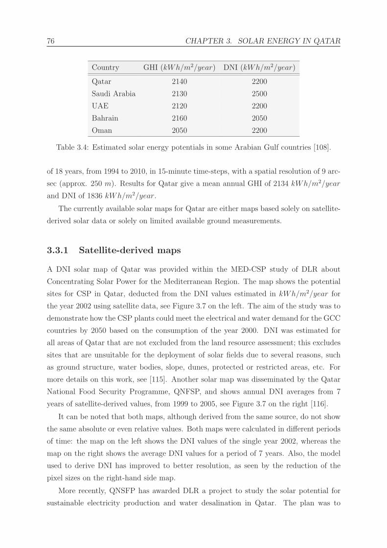
76 CHAPTER 3. SOLAR ENERGY IN QATAR
Country GHI (kWh/m2/year) DNI (kWh/m2/year)
Qatar 2140 2200
Saudi Arabia 2130 2500
UAE 2120 2200
Bahrain 2160 2050
Oman 2050 2200
Table 3.4: Estimated solar energy potentials in some Arabian Gulf countries [108].
of 18 years, from 1994 to 2010, in 15-minute time-steps, with a spatial resolution of 9 arc-
sec (approx. 250 m). Results for Qatar give a mean annual GHI of 2134 kWh/m2/year
and DNI of 1836 kWh/m2/year.
The currently available solar maps for Qatar are either maps based solely on satellite-
derived solar data or solely on limited available ground measurements.
3.3.1 Satellite-derived maps
A DNI solar map of Qatar was provided within the MED-CSP study of DLR about
Concentrating Solar Power for the Mediterranean Region. The map shows the potential
sites for CSP in Qatar, deducted from the DNI values estimated in kWh/m2/year for
the year 2002 using satellite data, see Figure 3.7 on the left. The aim of the study was to
demonstrate how the CSP plants could meet the electrical and water demand for the GCC
countries by 2050 based on the consumption of the year 2000. DNI was estimated for
all areas of Qatar that are not excluded from the land resource assessment; this excludes
sites that are unsuitable for the deployment of solar fields due to several reasons, such
as ground structure, water bodies, slope, dunes, protected or restricted areas, etc. For
more details on this work, see [115]. Another solar map was disseminated by the Qatar
National Food Security Programme, QNFSP, and shows annual DNI averages from 7
years of satellite-derived values, from 1999 to 2005, see Figure 3.7 on the right [116].
It can be noted that both maps, although derived from the same source, do not show
the same absolute or even relative values. Both maps were calculated in different periods
of time: the map on the left shows the DNI values of the single year 2002, whereas the
map on the right shows the average DNI values for a period of 7 years. Also, the model
used to derive DNI has improved to better resolution, as seen by the reduction of the
pixel sizes on the right-hand side map.
More recently, QNSFP has awarded DLR a project to study the solar potential for
sustainable electricity production and water desalination in Qatar. The plan was to

3.3. AVAILABLE SOLAR RESOURCE IN QATAR 77
DNI [kWh/m²/y]
DNI [kWh/m2/y]
Figure 3.7: DNI solar maps for Qatar from DLR. On the left, a map for the year 2002 for
the study of solar thermal electricity generating potentials in Qatar [115]. On the right,
a map for the period 1999-2005 [116].
combine accurate ground measurements, to be taken at several locations within Qatar,
and long-term historical satellite data (20 years) using the DLR service SOLEMI, in
order to have reliable information on GHI and DNI, to be then combined with data on
land use, infrastructure, soil condition, etc. within a Geographical Information System
(GIS) in order to identify suitable regions for future solar power plants in Qatar. The
project started in 2012. However, there is no access to information about the status of
the project.
High spatial (3×3 km2) and temporal (15-min) resolution satellite-derived solar maps
for Qatar can be purchased from any of the commercial satellite data providers, see Sec-
tion 1.5 for currently available services. One of these commercial companies, GeoModel
Solar, has published maps of DNI and GHI for several countries that can be downloaded
for free from their website; see Figure 3.8 for the SolarGIS DNI map of Qatar. Data can
also be obtained for free from several databases available on the internet, but at lower
resolution [70]. Maps of Qatar could also be derived from the solar mapping domain of
the neighbouring countries [117, 118].
On a larger regional scale, the Global Atlas for Renewable Energy, led by IRENA,

78 CHAPTER 3. SOLAR ENERGY IN QATAR
Figure 3.8: DNI solar map of Qatar by SolarGIS model from GeoModel Solar.
provides high-resolution and long-term solar resource maps. The database also includes
information on protected areas, roads or infrastructures, which enables to highlight po-
tential sites for developing solar projects and to undergo pre-feasibility studies. The
information provided using this database can be considered as a first estimation before
the initiation and the development of any solar-based project in the region, allows to
formulate policies in the renewable energy sector, and stimulates investment. The Solar
Atlas for the Mediterranean countries (Solar-Med-Atlas), although providing solar maps
for the Arab countries, does not have coverage of Qatar and the GCC area. Both the
Solar-Med-Atlas and the Global Atlas for Renewable Energy provide basic information on
solar radiation. Commercial companies and service providers focus more on customised
solutions and the provision of data time series and consultancy services for specific sites
and projects.
3.3.2 Ground measurement-derived maps
Currently, the only available direct measurements of solar resource throughout Qatar
consist of GHI data, being collected by the Qatar Meteorological Department (QMD),
which operates a network of 12 automatic weather stations (AWS) distributed across the
country, see Figure 3.9. Looking at the spatial distribution of the stations across the
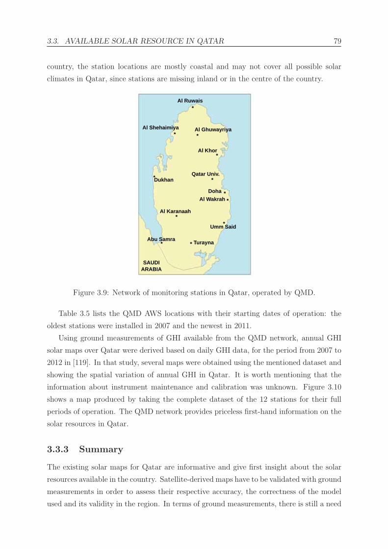
3.3. AVAILABLE SOLAR RESOURCE IN QATAR 79
country, the station locations are mostly coastal and may not cover all possible solar
climates in Qatar, since stations are missing inland or in the centre of the country.
*
*
*
*
*
*
*
*
*
*
*
*
Al Ruwais
DohaAl Wakrah
Abu Samra Turayna
Al Karanaah
Umm Said
Qatar Univ.Dukhan
Al Khor
Al GhuwayriyaAl Shehaimiya
SAUDIARABIA
Figure 3.9: Network of monitoring stations in Qatar, operated by QMD.
Table 3.5 lists the QMD AWS locations with their starting dates of operation: the
oldest stations were installed in 2007 and the newest in 2011.
Using ground measurements of GHI available from the QMD network, annual GHI
solar maps over Qatar were derived based on daily GHI data, for the period from 2007 to
2012 in [119]. In that study, several maps were obtained using the mentioned dataset and
showing the spatial variation of annual GHI in Qatar. It is worth mentioning that the
information about instrument maintenance and calibration was unknown. Figure 3.10
shows a map produced by taking the complete dataset of the 12 stations for their full
periods of operation. The QMD network provides priceless first-hand information on the
solar resources in Qatar.
3.3.3 Summary
The existing solar maps for Qatar are informative and give first insight about the solar
resources available in the country. Satellite-derived maps have to be validated with ground
measurements in order to assess their respective accuracy, the correctness of the model
used and its validity in the region. In terms of ground measurements, there is still a need

80 CHAPTER 3. SOLAR ENERGY IN QATAR
Station location Operating since Valid days (%)
1. Abu Samra 2007 95
2. Al Ghuwayriya 2009 98
3. Al Karanaah 2009 70
4. Al Khor 2007 97
5. Al Ruwais 2007 94
6. Al Shehaimiya 2011 100
7. Al Wakrah 2009 99
8. Doha 2008 93
9. Dukhan 2007 96
10. Qatar University 2007 99
11. Turayna 2011 99
12. Ummsaid 2007 99
Table 3.5: Solar monitoring stations collecting GHI in Qatar, with year of operation start
and percentage of days with daily values reported until 31 December 2012.
Figure 3.10: GHI solar map (values in kWh/m2/year) based on daily ground measure-
ments of GHI.
in Qatar to have precise measurements on the direct and the diffuse solar radiation, in
addition to the existing global radiation measurements.

Chapter 4
Instrumentation
This chapter presents the experimental setup with descriptions of all the instruments used
to collect the data used in this thesis. This includes a CL51 lidar ceilometer, from Vaisala,
used for the measurement of the backscatter coefficient of aerosols in the atmosphere, and
a Kipp & Zonen solar radiation monitoring station comprising several radiometers, used
for solar radiation measurements. In addition, the data acquisition system along with
examples of measurements as acquired by both systems are described. Details about the
experimental site and the features considered for its selection are also given.
4.1 Lidar-ceilometer
Previous studies have demonstrated that lidar systems are suitable devices for the detec-
tion of aerosol layers and their boundaries [120, 121]. The system works by transmitting
a laser pulse vertically into the atmosphere to measure the backscattered signals as ex-
plained in Section 2.3. The number of backscattering particles at a certain height from
the lidar determines the strength of the backscattered signal; for instance, higher amounts
of aerosols in the atmosphere will result in stronger backscatter signals. The distance is
determined by measuring the time of flight (TOF), i.e., the time between the transmis-
sion of the pulse and the reception of the signal. A ceilometer is a compact lidar system,
commercially available and designed in a way to operate continuously with little main-
tenance required. The primary use of a ceilometer is the detection of the heights of the
cloud base in the fields of aviation and meteorology. Beyond cloud detection, ceilometers
are also used for the determination of the boundary layer height and the characterisation
of its structure [122], monitoring of dust and volcanic ash clouds [123], and the estima-
tion of particulate matter (PM) concentration [124]. In this thesis work, however, the
lidar-ceilometer is not used for the determination of the height of the cloud base or the
81

82 CHAPTER 4. INSTRUMENTATION
boundary layer, but rather to measure the backscatter as a function of height in order
to get a quantitative indication on the amount of aerosols in the atmosphere. Below is a
description of the used ceilometer and its main specifications.
4.1.1 Vaisala ceilometer CL51
The detection of aerosols in the atmosphere was achieved with the CL51, an elastic lidar-
ceilometer commercially available from Vaisala, which in its customary usage provides
measurements of cloud heights and vertical visibility, through the acquisition of vertically-
resolved backscatter profiles of the atmosphere, including aerosols.
The CL51 unit was installed in December 2012 on the rooftop of the Qatar Environ-
ment and Energy Research Institute (QEERI) building in Doha. It has been operational
since then as part of the solar resource assessment and air quality monitoring facilities
at QEERI. A special platform was made for fixing it to the roof, to ensure its stability
against wind. The system is installed in one corner of the roof with no obstructions in
its field of view. The CL51 ceilometer consists of a shielding cabinet and a measurement
unit as shown in Figure 4.1.
Figure 4.1: Vaisala Ceilometer CL51, as installed at the QEERI facility in Doha, Qatar.
Inside the shield, there is a blower/heater to remove any excess of dust on the window,
and to ensure reliable operation in precipitation and extreme temperatures. The interior
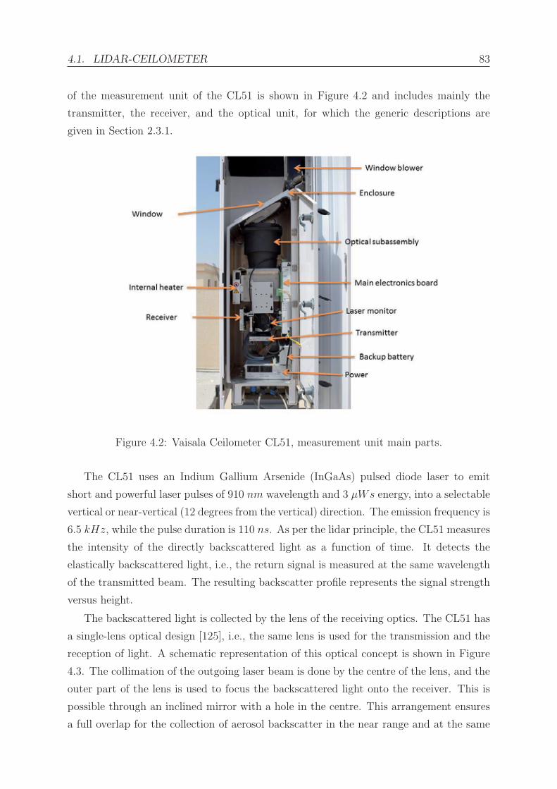
4.1. LIDAR-CEILOMETER 83
of the measurement unit of the CL51 is shown in Figure 4.2 and includes mainly the
transmitter, the receiver, and the optical unit, for which the generic descriptions are
given in Section 2.3.1.
Figure 4.2: Vaisala Ceilometer CL51, measurement unit main parts.
The CL51 uses an Indium Gallium Arsenide (InGaAs) pulsed diode laser to emit
short and powerful laser pulses of 910 nm wavelength and 3 μWs energy, into a selectable
vertical or near-vertical (12 degrees from the vertical) direction. The emission frequency is
6.5 kHz, while the pulse duration is 110 ns. As per the lidar principle, the CL51 measures
the intensity of the directly backscattered light as a function of time. It detects the
elastically backscattered light, i.e., the return signal is measured at the same wavelength
of the transmitted beam. The resulting backscatter profile represents the signal strength
versus height.
The backscattered light is collected by the lens of the receiving optics. The CL51 has
a single-lens optical design [125], i.e., the same lens is used for the transmission and the
reception of light. A schematic representation of this optical concept is shown in Figure
4.3. The collimation of the outgoing laser beam is done by the centre of the lens, and the
outer part of the lens is used to focus the backscattered light onto the receiver. This is
possible through an inclined mirror with a hole in the centre. This arrangement ensures
a full overlap for the collection of aerosol backscatter in the near range and at the same

84 CHAPTER 4. INSTRUMENTATION
Figure 4.3: Vaisala Ceilometer CL51, optical configuration. Image: Vaisala.
time makes the receiver practically blind to the light reflected by the lens. The good
overlap between the transmitted laser beam and the receiver field of view decreases the
effect of multiple scattering. The main characteristics and specifications of the CL51 are
listed in Table 4.1.
Property Value
Backscatter profiling range 15 km
Cloud reporting range 13 km
Reported vertical resolution 10 m
Measuring interval 6 s
Reporting interval 36 s
Laser type InGaAs diode
Laser wavelength 910 nm
Laser beam width at 7.5 km height 3 m
Laser beam width at 15 km height 6 m
Receiver Silicon avalanche photodiode
Pulse rate 6.5 kHz
Table 4.1: Specifications of the Vaisala ceilometer CL51 installed at the QEERI facility.
No specific maintenance is carried out on the CL51 other than daily cleaning of the
window so that it is kept clean, a requirement common to all optics.
4.1.2 Operating principle of CL51
The basic operating principle of the CL51 consists of the measurement of the time taken
by the pulse of light from its emission by the transmitter, through its way up to any

4.1. LIDAR-CEILOMETER 85
obstruction in the atmosphere until its detection by the receiver. This is schematically
illustrated in Figure 4.4. In this illustration, the obstruction is depicted by three layers
of cloud shapes. The basic formula relating the time delay t with the height h of the
backscatterer is given by:
h =ct
2, (4.1)
where c is the speed of light. For instance, a backscatter signal from a height of 7.5 km
will be received after 50.2 μs.
Figure 4.4: Vaisala Ceilometer CL51, principle of operation.
An example of measured signal as a function of height is shown in Figure 4.5 and
gives information about the presence of particles in the atmosphere which scatter the
light back from a certain height. The CL51 detection of the received light is based on the
photocurrent technique. The return signal is digitally sampled every 67 ns, which gives an
adequate spatial resolution of 10m for atmospheric measurements, up to 100 μs after each
pulse, providing a full range of operation up to 15 km. In the configuration of the CL51,
the transmitted laser power is low by design for safety and economic reasons, according to
the manufacturer; this makes the noise coming from the ambient light stronger than the
backscatter signal specially at the top heights. In order to reduce the noise, a signal-to-
noise ratio (SNR) improvement technique was adopted by Vaisala, and consists of sending

86 CHAPTER 4. INSTRUMENTATION
a large number of laser pulses and summing, for each height, all the return signals; the
noise, being random, adds up to a constant value lower and distinguishable from the
real signals, thus improving the SNR. Additional processing of the backscatter profile
provides the cloud base height detection. The detection of a cloud by the CL51 consists
of the identification of cloud droplet scattering that reduces the visibility to less than 100
m [126]. The CL51 cloud reporting range is up to 13 km, and it can detect up to three
layers of clouds in a simultaneous way. In case of precipitation or fog obscuring the cloud
base, the CL51 reports vertical visibility.
Figure 4.5: Example of a ceilometer measurement signal.
Based on the lidar equation (Equation 2.21), the instantaneous return signal power
can be derived. This is given by:
Pr(Z) = E0c
2
A
Z2β(Z) exp
[−2
∫ Z
0
σ(Z ′)dZ ′], (4.2)
where Pr(Z) is the instantaneous power received from distance Z, E0 is the effective
pulse energy taking all optics attenuation into account and given in Ws, c is the speed
of light in m/s, A is the receiver aperture in m2, Z is the distance in m, β(Z) is the
volume backscatter coefficient at distance Z in m−1srad−1 which represents the part of
light reflected back towards the receiver from a distance Z, and the exponential term is
the attenuation of the light from the two-way travel of the light: the transmitted and
backscattered light. The return signal is multiplied with the square of the height in order
to have a normalised signal and to eliminate the height dependence of the power of the
return signal. This normalisation, however, accentuates the noise with increasing height
since the noise is height-independent. In the processing of the CL51 data and in order
to solve the lidar equation, the backscatter coefficient is considered proportional to the

4.1. LIDAR-CEILOMETER 87
extinction coefficient and expressed as follows:
β(Z) = kσ(Z), (4.3)
where k is the proportionality constant in 1/srad, also known as lidar ratio.
For solving the lidar equation for the CL51, it is assumed that the lidar ratio k
remains constant with height, specially since it is needed to have accurate estimates of
the extinction profile. In many cases, it has been demonstrated that k is equal to 0.03,
smaller in high humidity conditions (around 0.02), and bigger (up to 0.05) in low humidity
conditions [126]. However, in precipitation conditions, k can have a wider range of values.
4.1.3 Maintenance
The CL51 is a self-operating device and once installed, there is basically no need for
adjustments in the field. The embedded software of the CL51 includes self-monitoring
controls and functions meant for testing and maintenance purposes and gives continuous
status information. This includes internal tests of the laser power, receiver sensitivity,
internal voltages, window contamination, internal temperatures, etc.. Any failure of these
tests will indicate an error in the status message with the error type and information.
The CL51 is fitted with a maintenance terminal connection; in case any maintenance is
needed it is possible to connect a serial cable to the ceilometer maintenance port and a
terminal computer in order to access the CL51 maintenance open command. A built-in
tilt angle sensor detects the angle of deviation from the vertical; this automatic tilt angle
measurement triggers a correction of the tilt accordingly. As seen in Figure 4.2, the CL51
is also fitted with a window blower which runs when the system detects contamination of
the window; the blower only removes small contamination from the window and dries off
rain drops. The proper functioning of the blower is automatically checked once an hour.
The only daily maintenance activities carried out on the CL51 are: the manual cleaning
of the window so that it is kept clean, as applicable to all optics, and the checking
on the proper operation of the blower. Additional controls carried out daily include
inspection of the data acquisition software to look for any data interruption caused by
data transmission or collection failure, and checking the data message for alarms and
warnings.
4.1.4 Data collection
For the data acquisition, the CL51 was connected to a PC through an RS-232 serial cable.
Two supporting software packages can be used with the CL51: CL-VIEW, a graphical

88 CHAPTER 4. INSTRUMENTATION
user interface for collected data, and BL-VIEW, the boundary layer analysis tool.
The CL-VIEW software is a graphical presentation program for cloud height and
backscatter profile data as measured by the ceilometer. It is used for collecting, storing
and presenting the data acquired by the CL51. In its online mode, CL-VIEW collects the
data from the ceilometer via the serial line and stores them on the computer hard disk ac-
cording to the selected options. The data are displayed instantaneously in graphical form
on the screen. CL-VIEW can also be used to examine stored data, in its offline mode. In
Figure 4.6, an example is shown of the so-called ‘cloud intensity’ graph and a backscatter
data profile collected at the experimental site in Doha, Qatar, on 07/Jun/2013, during
the normal operation of the CL51. The plot on the left corresponds to the cloud intensity
graph and is used for the cloud height determination. The horizontal axis in the plot
presents the time and the vertical axis is the altitude. Each point reflects the place of
the backscatter identified by the current time. The darkness in the colour of the points
identifies the intensity of the backscatter at the corresponding height. The plot on the
right is the backscatter profile; this can be presented as an instantaneous or as averaged
mode. The horizontal axis is the backscatter intensity and the vertical axis is the alti-
tude. In the offline mode of CL-VIEW, each data file contains all information about the
backscatter coefficients acquired as a function of height and time and are used for the
further analysis of the atmospheric backscatter coefficient, of interest in this work.
CL-VIEW - Port 1 [C:\clviewlogs\201306\A3060700.DAT], 07/07/2014 10:01:55
Figure 4.6: CL-VIEW cloud and backscatter intensity graphs as measured by the Vaisala
Ceilometer CL51. Data collected on 07/Jun/2013.
BL-VIEW is a software tool used for boundary layer reporting and analysis. It can be

4.1. LIDAR-CEILOMETER 89
used instead of CL-VIEW for collecting, storing, and presenting the data acquired by the
CL51. BL-VIEW analyses the ceilometer backscatter profile data according to default
parameters and reports the height of the planetary boundary layer and of other aerosol
layers from ground level (the height of the ceilometer) up to 4 km. Indeed, the measured
backscatter profile gives information about the presence of aerosols in the atmosphere
which are mainly emitted at the surface and have in general a higher concentration
within the boundary layer than in the free troposphere. Therefore, a sharp gradient in
the aerosol concentration detected by the backscatter signal indicates the height of the
boundary layer and separates it from the relatively clean free troposphere. The algorithm
uses an enhanced gradient method approach. The standard gradient method consists of
searching for strong gradients or local gradient minima in the backscatter profile [127].
The most pronounced of the found minima is reported as the boundary layer height by
the method, and the other minima can be reported as residual or additional layers. The
BL-VIEW algorithm involves: cloud and precipitation filter, noise- and range-dependent
time- and height-averaging intervals, and signal strength-dependent detection thresholds.
Averaging in time and height is applied in order to reduce sensitivity to noise and weather
conditions. Additional filters are also applied for the enhancement of the retrieval of the
boundary layer specially in situations when weather conditions such as precipitation or
fog prevent the detection of boundary layer height [128]. BL-VIEW can report up to
three layer heights in a single vertical measurement. Figure 4.7 shows samples of BL-
VIEW backscatter profiles for cloudless days, as measured by the CL51, over Doha for
several days in different months, covering varying degrees of dust in the atmosphere.
Each of these plots displays the evolution of the backscatter signal during one full day,
from midnight to midnight. The colours represent the intensity of the signal (left side
scale), from dark blue for the lowest and red for the highest intensities. The vertical axis
on the right side indicates the height above ground level from 0 to 4000 m. The black
squares are layer boundaries found by the gradient algorithm of BL-VIEW. For instance,
on 12 January and 26 March, the PBL is relatively well defined since a layer can be
found with an evolution through the day from sunrise to sunset as per the definition of
the boundary layer. On the 2nd of January, the boundary layer can still be found but
other layers are also evident. On the 27th of May, the boundary layer is being pushed
down by a thick layer of dust on top of it. On the 12th and 22nd of May, the dust layer
is so dense and dominant that the boundary layer signal cannot be differentiated from
other layers. Many days in April and May 2013 were loaded with heavy dust and the
corresponding BL-VIEW graphs are similar to the ones seen in this figure, with the dust
layer extending above 4000 m. An attempt was made [129] to compare the boundary

90 CHAPTER 4. INSTRUMENTATION
layer height with DNI measurements at noon. The study had inconclusive results because
the BL height could not be identified with BL-VIEW from other dust layers, which often
extended above 4 km, in many days.
Figure 4.7: Samples of backscatter profiles as displayed by BL-VIEW.
4.1.5 Data used
Different intensity profiles can be recorded by the CL51 depending on the constituents
of the atmosphere, like dust, fog, haze, rain, etc. These profiles provide information on
the height of the cloud base as a function of time, given by CL-VIEW, and data on
the evolution and structure of the boundary layer height, given by BL-VIEW. Of most
importance for this work are the backscatter coefficients retrieved by the ceilometer,
which are recorded as a function of time and height according to Equation 4.2. The data
analysis presented here uses the CL51 signal describing the backscatter properties of the
atmosphere. These signals are represented as a two-dimensional dataset of backscatter
coefficient values, reported in time every 36 s, and height up to 15 km in 10-m steps.

4.2. SOLAR RADIATION INSTRUMENTS 91
4.2 Solar radiation instruments
For the precise measurements of solar radiation, a Kipp & Zonen solar radiation monitor-
ing station has been installed in QEERI’s facilities and is acquiring data since December
2012. This monitoring station consists of a SOLYS 2 sun tracker which hosts all the
instruments for solar radiation measurements: one CHP1 pyrheliometer for the measure-
ment of direct normal irradiance mounted in a way to follow the sun rays all through
the day and all through the year, and two CMP11 pyranometers, one shaded for the
measurement of the diffuse horizontal radiation and one unshaded for the measurement
of the global horizontal radiation, both mounted on a horizontal platform which ensures
the mechanical stability and proper levelling of the instruments. Another instrument,
a CGR4 pyrgeometer, was also mounted on the monitoring station for measuring the
infrared radiation. However, the CGR4 measurements are not used in the scope of this
work. The Kipp & Zonen type of station is widely used for high quality solar measure-
ments and was selected for its high performance and reliability and its compliance with
the requirements of the BSRN, which uses Kipp & Zonen sun trackers and radiometers
in many of their stations installed worldwide. Figure 4.8 shows the complete monitoring
station with all the mounted accessories and instruments as installed and operating at
QEERI’s facility. Below is a description of each of these instruments.
4.2.1 SOLYS 2 sun tracker
The SOLYS 2 is a fully automatic two-axis sun tracker, used as a platform for posi-
tioning the radiometers that need to follow the movement of the sun in the sky. It has
an integrated GPS receiver; the measurement site’s latitude, longitude and time were
automatically configured by the GPS during installation and the time is being regularly
updated by the GPS to avoid any internal clock drift. An on-board program, the Michal-
sky algorithm [130], uses this information to calculate regularly the position of the sun
throughout the day. The pointing accuracy of the SOLYS 2 is 0.1◦, which meets the
BSRN requirements. As additional control for the accuracy of the tracking, the SOLYS 2
was fitted with a sun sensor kit consisting of a four-quadrant photodiode sensor within a
weather resistant enclosure. This sensor provides active tracking, and corrections to the
tracking algorithm, in case the mounting of the tracker is not stable or exhibits move-
ment. For the installation of the tracker, the tripod stand with levelling feet was bolted
on a firm and stable base. The levelling and alignment adjustments were aided by an
integrated bubble level on the top of the tracker. The obstacle-free operating area of
SOLYS 2, including all accessories, ensures a proper movement for the SOLYS 2 and

92 CHAPTER 4. INSTRUMENTATION
Figure 4.8: Solar radiation monitoring station as installed at the QEERI facility in Doha,
Qatar.
prevents any blocking, with respect to both the azimuth and zenith axes, throughout the
year. On the sides of the tracker there are plates with zenith adjustment for the mounting
of the pyrheliometer, so that it points precisely to the sun, and for the shading assem-
bly which serves to ensure blocking the direct radiation from reaching the pyranometer
measuring the diffuse radiation. On the top, a horizontal platform is fitted in order to
conveniently mount the other radiometers. The tracker uses stepping motors controlled
by micro-processors to make the horizontal (azimuth) and vertical (zenith) movements
in a way to follow the solar arc. The main specifications of the SOLYS 2 system are
summarised in Table 4.2.
4.2.2 CHP1 pyrheliometer
For measuring DNI, the Kipp & Zonen CHP1 pyrheliometer was used; this device com-
plies with the ISO and WMO performance criteria for First Class Normal Incidence
Pyrheliometers, classifications described in Section 1.3. It is calibrated by Kipp & Zo-
nen upon manufacturing and a calibration certificate traceable with the WRR (World
Radiometric Reference) is supplied with the instrument, indicating the sensitivity of the
pyrheliometer, which is the constant proportionality ratio between the voltage output

4.2. SOLAR RADIATION INSTRUMENTS 93
Property Value
Pointing accuracy < 0.1◦
Torque 20 Nm
Angular velocity 5◦/s
Rotation 110◦ zenith and 540◦ azimuth
Over rotation and damage protection Physical limits stop
Operating temperature range -40 ◦C to 50 ◦C (AC power with heater)
Bubble level accuracy < 0.1◦
Supply voltage 28–30 VDC (nominal 24 DC)
90–264 VAC (50/60 Hz)
Table 4.2: Main specifications of Kipp & Zonen SOLYS 2, installed at the QEERI facility.
and an absolute irradiance level. The sensitivity used hereby, as given by the calibration
certificate from Kipp & Zonen, is 7.75 μV/(W/m2), valid for an ambient temperature
of 22 ± 2 ◦C and a normal incident radiation of 500 W/m2. This factor is determined
indoors in Kipp & Zonen laboratories by comparing the CHP1 against a reference pyrhe-
liometer of similar type, in a horizontal parallel beam of light from a xenon lamp. The
used reference pyrheliometer is fully characterised in terms of linearity, temperature de-
pendence and directional response and is regularly calibrated outdoors, using the sun as
source, at the World Radiation Centre in Davos, Switzerland with a calibration accuracy
of ±0.5%. The CHP1 measures the irradiance resulting from the radiant flux from a
solid angle of 5◦. Figure 4.9 shows the CHP1 as mounted on the SOLYS 2 at QEERI.
The CHP1 has a flat window made of quartz, which ensures that 97 to 98% of the solar
radiation spectrum will be transmitted across the window to reach the detector. A rain
shield cover protects the window. The instrument temperature is measured through 2
thermistors placed inside the device assembly. The two alignment aids on the pyrheliome-
ter tube are used for checking the alignment the CHP1 with the axis of the direct beam
of the sun. The detection in the CHP1 is based on the thermoelectric effect described in
Section 1.3.1. It consists of the thermopile with black surface coating on the top, with a
spectral selectivity of less than 2%. The optical configuration of the CHP1 complies with
the WMO recommendations; it consists of a field stop, sets of blackened baffles and an
aperture stop, defining the CHP1 field of view of 5◦ and slope angle of 1◦. The detector
sits behind the aperture stop. The interior of the CHP1 tube, which surrounds and holds
this assembly, is blackened. For the prevention of dew on the inner sides of the window
in case moisture enters the radiometer body, a screw-in drying cartridge is mounted in
the radiometer housing and filled with silica gel.

94 CHAPTER 4. INSTRUMENTATION
Figure 4.9: Kipp & Zonen CHP1 pyrheliometer used at the solar radiation monitoring
station installed at the QEERI facility.
The parameters characterising the response of the CHP1 are provided in Table 4.3,
which also summarises its main specifications. Kipp & Zonen expects a maximum uncer-
tainty of 2% for hourly totals and 1% for daily totals for the CHP1 pyrheliometer.
4.2.3 CMP11 pyranometer
The pyranometers used for measuring global and diffuse solar radiation are the CMP11
model from Kipp & Zonen, which fully complies with the requirements of ISO 9060:1990
for a Secondary Standard Pyranometer; the two units are shown in Figure 4.10. The
CMP11 is calibrated in accordance with ISO 9847 for the calibration of field pyranometers
by comparison to a reference pyranometer and is supplied with the calibration certificate.
The CMP11 pyranometer is designed for measuring the short-wave total solar irradiance,
which is the sum of the direct and diffuse solar radiation, on a plane surface inW/m2. Like
the CHP1, the CMP11 uses the thermoelectric effect and has a 32-junction thermopile
sensing element, with a non-spectrally selective black surface coating on the top of it. It is
also fitted with a built-in passive temperature compensation system with a standardised
linear function. The sensing element characterises the detector in terms of response
time, linearity and measurement range. The detector is shielded by two glass domes

4.2. SOLAR RADIATION INSTRUMENTS 95
Property Value
ISO Classification First class
Response time (95%) 5 s
Zero offsets due to temperature change (5 K/hr) ±1 W/m2
Non-stability (change/year) ±0.5%
Non-linearity (0 to 1000 W/m2) ±0.2%
Temperature dependence of sensitivity 0.5% (-20 ◦C to 50 ◦C)
Sensitivity 7 to 14 μV/(W/m2)
Impedance 10 to 100 Ω
Operating temperature -40 ◦C to 80 ◦C
Spectral range 200 to 4000 nm
Typical signal output for atmospheric applications 0 to 15 mV
Maximum irradiance 4000 W/m2
Expected daily uncertainty ±1%
Full opening view angle 5◦ ± 0.2◦
Slope angle 1◦ ± 0.2◦
Required tracking accuracy ±0.5◦
Table 4.3: Main specifications of Kipp & Zonen CHP1, installed at the QEERI facility.
for additional protection of the sensing element and the black painted coating. The
glass domes are designed to minimise errors in measurement at all incident angles (the
directional response) and allow the transmittance of 97 to 98% of the solar radiation
spectrum. A built-in bubble level is used for checking the alignment of the instrument.
The CMP11 is placed horizontally on the mounting stand through its three feet, of which
two are adjustable in order to properly level the detector surface; this is achieved by
turning the two adjustable feet to bring the bubble of the spirit level centrally within a
marked ring. A sun shield is used to cover the housing and reduce solar heating. No
power is required for the operation of the CMP11; the radiation absorbed by the sensing
element produces a small analogue output voltage. Similarly to the CHP1, the CMP11
has a removable drying cartridge filled with self-indicating silica gel desiccant used to
absorb the humidity within the radiometer so that the detector and electronics of the
CMP11 are kept dry. For the diffuse measurements, a shading mechanism consisting
of a small sphere mounted on an articulated assembly was installed on the SOLYS 2
sun tracker. The sphere casts a shadow adjusted properly upon installation to cover
the pyranometer dome completely. For improving the accuracy of the measurements
and to better adapt to the dusty and humid weather conditions of Qatar, both CMP11

96 CHAPTER 4. INSTRUMENTATION
pyranometers, for global and diffuse measurements, were fitted with ventilation units
running continuously to keep the domes cleaner. This decreases the level of dirt and
condensation on the dome and lowers the thermal offset in the dome, characteristic of
the pyranometer. All instruments were grounded for lightning and signal noise protection.
Figure 4.10: Kipp & Zonen CMP11 pyranometers used at the solar radiation monitoring
station installed at the QEERI facility. Note the shadow covering the sensor of the left
pyranometer, in order to measure DHI.
The physical properties are listed in Table 4.4; they are similar to those for the CHP1,
except for the zero offset A and the directional response, which only apply to the CMP11
pyranometer.
Based on many years of field measurements, Kipp & Zonen empirically determines
uncertainty figures of their pyranometers, for typical operating conditions. For a high
quality pyranometer the WMO expects maximum uncertainty totals of 3% in the hourly
radiation. In the daily total an uncertainty of 2% is expected, since some response
variations cancel each other out if the integration period is long [22].
The sensitivity of the CMP11 measuring the global radiation in the QEERI station
is 8.78 μV/(W/m2) and the sensitivity of the CMP11 measuring the diffuse radiation is
8.47 μV/(W/m2) at normal incidence on horizontal pyranometer, obtained by comparison
to a reference pyranometer’s readings, and supplied on the calibration certificate. The
calibration procedure is carried out indoors in Kipp & Zonen laboratories following [31],
and is based on a side-by-side comparison of the CMP11 pyranometer with a reference
pyranometer under a stable artificial sun corresponding to a metal-halide high-pressure
gas discharge lamp; the irradiance at the radiometers is approximately 500 W/m2. The
reference pyranometers used by Kipp & Zonen are regularly calibrated outdoors at the
WRC, using the ‘continuous sun-and-shade’ method. They are also fully characterised
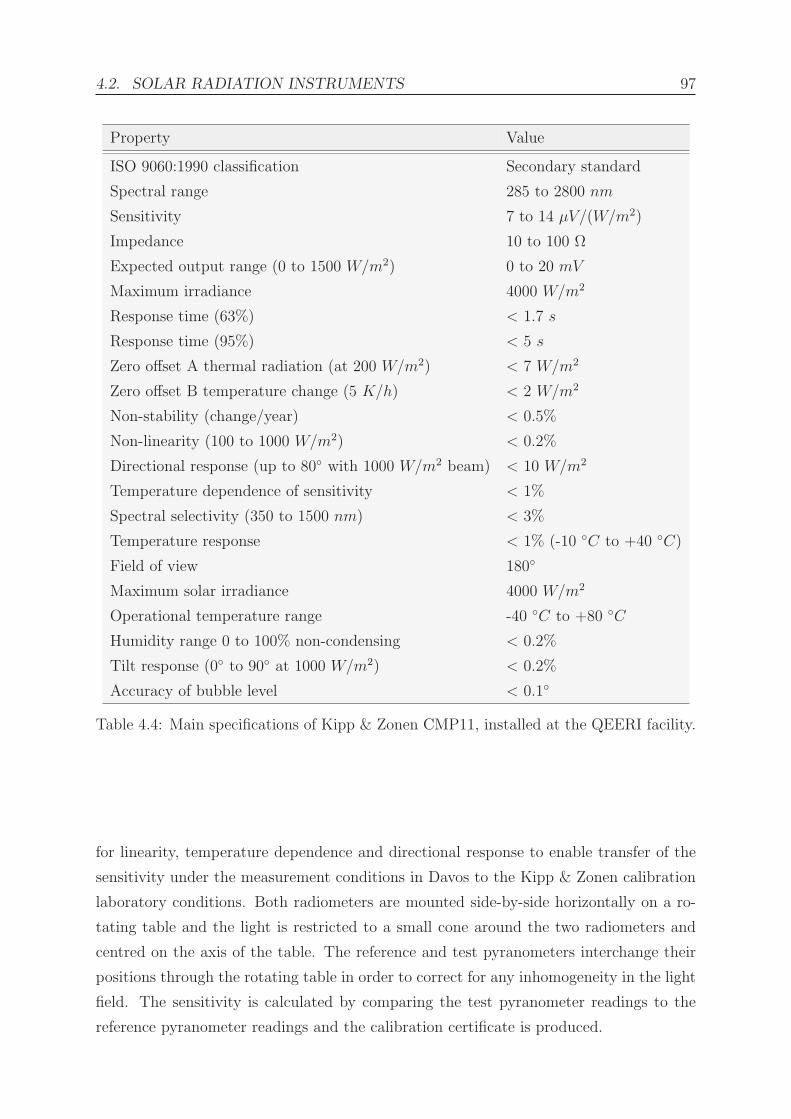
4.2. SOLAR RADIATION INSTRUMENTS 97
Property Value
ISO 9060:1990 classification Secondary standard
Spectral range 285 to 2800 nm
Sensitivity 7 to 14 μV/(W/m2)
Impedance 10 to 100 Ω
Expected output range (0 to 1500 W/m2) 0 to 20 mV
Maximum irradiance 4000 W/m2
Response time (63%) < 1.7 s
Response time (95%) < 5 s
Zero offset A thermal radiation (at 200 W/m2) < 7 W/m2
Zero offset B temperature change (5 K/h) < 2 W/m2
Non-stability (change/year) < 0.5%
Non-linearity (100 to 1000 W/m2) < 0.2%
Directional response (up to 80◦ with 1000 W/m2 beam) < 10 W/m2
Temperature dependence of sensitivity < 1%
Spectral selectivity (350 to 1500 nm) < 3%
Temperature response < 1% (-10 ◦C to +40 ◦C)
Field of view 180◦
Maximum solar irradiance 4000 W/m2
Operational temperature range -40 ◦C to +80 ◦C
Humidity range 0 to 100% non-condensing < 0.2%
Tilt response (0◦ to 90◦ at 1000 W/m2) < 0.2%
Accuracy of bubble level < 0.1◦
Table 4.4: Main specifications of Kipp & Zonen CMP11, installed at the QEERI facility.
for linearity, temperature dependence and directional response to enable transfer of the
sensitivity under the measurement conditions in Davos to the Kipp & Zonen calibration
laboratory conditions. Both radiometers are mounted side-by-side horizontally on a ro-
tating table and the light is restricted to a small cone around the two radiometers and
centred on the axis of the table. The reference and test pyranometers interchange their
positions through the rotating table in order to correct for any inhomogeneity in the light
field. The sensitivity is calculated by comparing the test pyranometer readings to the
reference pyranometer readings and the calibration certificate is produced.

98 CHAPTER 4. INSTRUMENTATION
4.2.4 Data collection
The data acquisition system is the COMBILOG data logger provided by Kipp & Zonen
and manufactured in Germany by Theodor Friedrichs & Co. This logger is placed inside
a weatherproof stainless steel enclosure suitable for outdoor use (see Figure 4.11) and can
handle up to 8 analogue signal inputs. For the configuration of the present solar station, 6
of these analogue inputs were used. The COMBILOG operates using a 12 V power supply
which fits in the same enclosure of the logger and allows the connection to the mains (AC
power). A supply of 12 V DC from a solar panel is also used as a back-up supply with
a battery placed inside the enclosure for a potentially unreliable supply. The data and
configuration in the COMBILOG are non-volatile and are retained if the power goes off.
Each time data are downloaded, they are deleted from the internal memory of the logger.
Due to this, an external memory card was used as a backup. The sampling happens every
second and the stored data are one-minute averages. Although the connection between
the COMBILOG and the PC where data are downloaded and monitored can be made
wirelessly via a GPRS/GSM modem, in this case it is made through an RS-232 serial
cable, since the distance between the PC and the logger is short (less than 10 m). The
clock of the data logger is automatically synchronised with the computer clock after each
data retrieval, and the PC clock is routinely verified for drifts using the clock of another
instrument updated by a GPS receiver.
For the setup and configuration of the logger, a specific MS Windows software (called
COMBILOG) is used, where live data can be viewed but not stored at the same time.
However, a manual download of the data is possible. Within the software, each measuring
channel is defined as a variable in a variable table. The used sensors are selected from an
integrated database and the linearisation of the sensor signals is performed automatically.
Another software package, COMGRAPH, is used for data logging; COMGRAPH allows
the scheduling of automatic downloads of the data and it also produces graphs and basic
analysis of the stored data. Data are stored as text files. The data logger uses the
instrument calibration factors (sensitivity) embedded in the library of the software to
convert the input voltages into radiation values in W/m2 according to:
E =U
S, (4.4)
where U is the output signal of the radiometer in μV and S is the sensitivity in μV/(W/m2).
The COMGRAPH software is used for quick visualisation and daily checks of the
data. The graphical representation of each of the solar radiation components is shown
individually, and there is no means to include the three plots on the same graph. However,
for the data analysis done in this thesis, all data are exported to text files, processed and

4.2. SOLAR RADIATION INSTRUMENTS 99
Figure 4.11: Data logger in its enclosure, for the communication of the solar radiation
measurements from the monitoring station installed at the QEERI facility.
cleaned to be used in C++ macros conceived specifically to apply thorough quality check
procedures to the data and for the calculation of the hourly, daily and monthly averages
of solar radiation, as well as the other analyses. As an example of the data analysis of the
three components, profiles of 1-minute DNI, GHI and DHI collected at the experimental
site are shown in Figure 4.12, including cloudy days (7–8 May 2013), clear days (9–11
May 2013), one day with haze (6 May) and days with dust (7–9 June 2013).
4.2.5 Installation and operation site
The solar monitoring station was installed on the rooftop of a building of QEERI’s offices,
at a latitude of 25.33◦ N and longitude of 51.43◦ E. The site was carefully prepared before
the installation of the monitoring station. The location on the roof where the solar
monitoring station is installed was selected to be as much as possible free of obstructions
to the hemispherical view as seen from the plane of the detectors of the radiometers, to
eliminate any shadow casting upon any of the instruments at any time and enough free
space for the movement of the sun tracker. A raised metallic structure was specifically
built and serves as a solid and stable horizontal platform for mounting the SOLYS 2
tripod. The dimensions of the base are 1 × 1 m2 with 65 cm height. Three holes were

100 CHAPTER 4. INSTRUMENTATION
9/May/2013 10/May/2013 11/May/2013
]2Ir
radi
ance
[w/m
0
200
400
600
800
1000 DNIGHIDHI
6/May/2013 7/May/2013 8/May/2013
]2Ir
radi
ance
[w/m
0
200
400
600
800
1000 DNIGHIDHI
7/June/2013 8/June/2013 9/June/2013
]2Ir
radi
ance
[w/m
0
200
400
600
800
1000 DNIGHIDHI
Figure 4.12: Data analysis of DNI, GHI and DHI measured at the experimental site in
Doha, Qatar, for clear days (9–11 May), cloudy days (7–8 May), with rain (8 May), with
haze (6 May) and days with dust (7–9 June).
drilled for fixing down (bolting) securely the tripod legs of the SOLYS 2 as per the
specifications given by the manufacturer. A power connection for the SOLYS 2 was
provided. Proper electric grounding was considered for all the instruments during the
installation. All the cables connecting the instruments to the data logger are shielded
and were provided by the manufacturer.
Daily checks were scheduled for routine maintenance of the instruments; this was
possible because of the easy and safe access to the instruments and the near proximity
of a control room hosting the PCs of data collection and visualisation. The daily checks
include:
• Cleaning the dome of the pyranometers and the window of the pyrheliometer.
• Checking the levelling of the pyranometers and the alignment of the pyrheliometer.
• Checking the levelling of the sun tracker.
• Checking the drying cartridges and that the silica gel is still active.
• Checking the position of the shadow on the pyranometer of the diffuse measure-
ments.
4.2. SOLAR RADIATION INSTRUMENTS 101
• Checking that the data is properly collected and downloaded from the logger.
• Visual checking of the data in daily profiles to spot any problems.
When the yellow silica gel in the drying cartridge is turned completely transparent,
it is replaced by fresh silica gel supplied in small refill packs by Kipp & Zonen. At the
same time it is checked that the radiometer mounting is secure and that the cables are in
good condition. The replacement of the desiccant by fresh silica was made approximately
every 2 to 3 months.
All these checks, as well as any maintenance work or changes done on the instruments,
were recorded on a log book kept in the control room, with the date and time and the
associated activity performed. This recording is very important, since it helps in the
process of identification of problems when bad data are identified and flagged during the
data quality control. By examining the log file, any activity that might have influenced
the data for the time and date specified by the quality control can be spotted.
4.2.6 Data quality control
While direct measurements are the best method for the knowledge of solar radiation data,
errors can be expected, as in any type of measurements. Solar radiation measurements, in
particular, are more likely to have errors than the measurements of other meteorological
parameters [131], and it is possible to have questionable values even when maintenance
and all necessary controls were undertaken prior to the recording of the data. The sources
of errors in solar radiation measurements can be divided into two categories: equipment
errors and uncertainty, and operation-related problems and errors [132].
In order to make sure that all measured data are reliable, several procedures and
software have been developed for post-measurement quality assessment of solar data [133,
134, 135]. For instance, SERI QC [136] is a procedural and software package developed by
NREL for quality assessment of data obtained from one-minute to one-hour integrations
of the three solar radiation data elements (global horizontal, diffuse horizontal, and direct
normal irradiance), defining ranges of acceptable data based on dimensionless parameters
normalised with respect to extraterrestrial radiation. The Baseline Surface Radiation
Network also has recommendations for radiation data quality checks [137]. The BSRN
recommendations were adopted in this research work to ensure the reliability of the
acquired data before further processing. The BSRN data quality control includes the
following checks:
• Checking whether the measured data do not exceed physically possible limits, which
are estimated or defined limits based on basic physical principles. For instance, the

102 CHAPTER 4. INSTRUMENTATION
direct normal irradiance should not be less than zero or greater than the extrater-
restrial value. The global horizontal irradiance should not be greater than the
horizontal component of the extraterrestrial beam. The diffuse irradiance should
not exceed the expected Rayleigh diffuse sky. By applying this test, it is possible
to spot problems such as the misalignment of the tracker or a dirty pyrheliome-
ter window, and identify thermal offset problems as described in Section 1.3. In
some rare situations, the measured value, while correct, may exceed the possible
physical limits; this can be due to severe refraction processes, multiple reflections
between broken clouds and bright surfaces, inversions, night-time offsets, tempera-
ture jumps, etc. [138]. Therefore, a visual inspection and a qualitative assessment
of the data is always required for confirmation.
• Checking whether the measured data do not exceed extremely rare limits; these lim-
its have been defined based on the use of meteorological theory and experience, and
the analysis of distributions, climatological statistics and extreme weather events
[139].
• Checking how the measured data should compare to each other. This consistency
check verifies the relationship between the three components (GHI, DHI and DNI)
based on Equation 1.11. If the values agree within a few percent, it is likely that
the three of them are correct, if not it is likely that one or more of them were poorly
measured or the solar tracker was not pointing correctly to the sun. Another test is
to check the so-called diffuse ratio, DHI/GHI, to ensure that the diffuse component
does not exceed the total radiation.
Table 4.5 resumes the applied physically possible and extremely rare limits tests, and
Table 4.6 resumes the consistency checks (the interrelation between the three components
and the conditions for the diffuse ratio).
Minp Maxp Mine Maxe
DNI -4 W/m2 Sa -2 W/m2 Sa · 0.95 · μ0.20 + 10 W/m2
GHI -4 W/m2 Sa · 1.5 · μ1.20 + 100 W/m2 -2 W/m2 Sa · 1.2 · μ1.2
0 + 50 W/m2
DHI -4 W/m2 Sa · 0.95 · μ1.20 + 50 W/m2 -2 W/m2 Sa · 0.75 · μ1.2
0 + 30 W/m2
Table 4.5: Quality controls as defined by the BSRN recommendations. The lower physi-
cally possible (Minp) and extremely rare (Mine) limits, and the corresponding maximum
limits (Maxp and Maxe) are defined for DNI, GHI and DHI. Sa is the solar constant ad-
justed for the earth-sun distance and μ0 = cos(θz) is the cosine of the solar zenith angle.
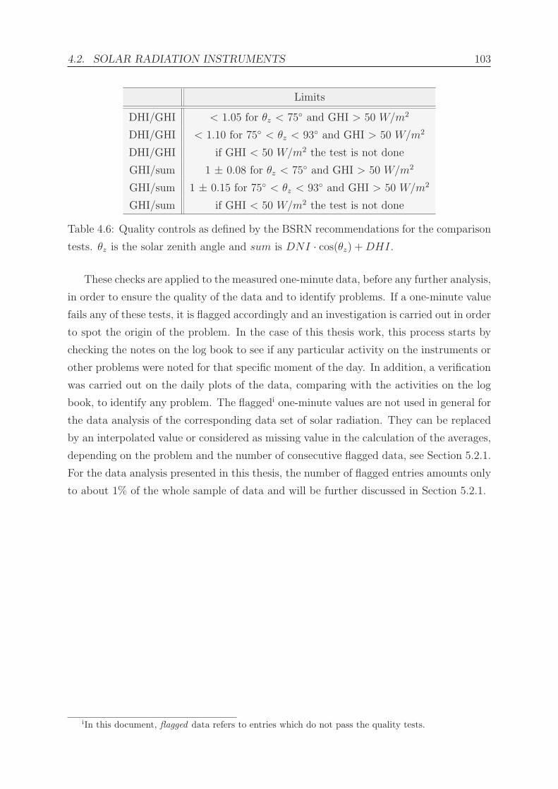
4.2. SOLAR RADIATION INSTRUMENTS 103
Limits
DHI/GHI < 1.05 for θz < 75◦ and GHI > 50 W/m2
DHI/GHI < 1.10 for 75◦ < θz < 93◦ and GHI > 50 W/m2
DHI/GHI if GHI < 50 W/m2 the test is not done
GHI/sum 1 ± 0.08 for θz < 75◦ and GHI > 50 W/m2
GHI/sum 1 ± 0.15 for 75◦ < θz < 93◦ and GHI > 50 W/m2
GHI/sum if GHI < 50 W/m2 the test is not done
Table 4.6: Quality controls as defined by the BSRN recommendations for the comparison
tests. θz is the solar zenith angle and sum is DNI · cos(θz) +DHI.
These checks are applied to the measured one-minute data, before any further analysis,
in order to ensure the quality of the data and to identify problems. If a one-minute value
fails any of these tests, it is flagged accordingly and an investigation is carried out in order
to spot the origin of the problem. In the case of this thesis work, this process starts by
checking the notes on the log book to see if any particular activity on the instruments or
other problems were noted for that specific moment of the day. In addition, a verification
was carried out on the daily plots of the data, comparing with the activities on the log
book, to identify any problem. The flaggedi one-minute values are not used in general for
the data analysis of the corresponding data set of solar radiation. They can be replaced
by an interpolated value or considered as missing value in the calculation of the averages,
depending on the problem and the number of consecutive flagged data, see Section 5.2.1.
For the data analysis presented in this thesis, the number of flagged entries amounts only
to about 1% of the whole sample of data and will be further discussed in Section 5.2.1.
iIn this document, flagged data refers to entries which do not pass the quality tests.

104 CHAPTER 4. INSTRUMENTATION

Chapter 5
Solar Radiation Data Analysis
As discussed in Chapter 2, when solar radiation passes through the earth’s atmosphere,
it is modified by absorption and scattering processes, resulting in different amounts and
qualities of solar radiation reaching the earth’s surface. This variation depends on the
location on earth, and on the incident angle of the solar radiation. For better understand-
ing of the solar energy in Doha, at the experiment site, it is necessary to characterise it
and estimate its variations using the past and the current recorded data. A description of
the Qatar Meteorological Department’s automatic weather stations network is given first.
Then, an analysis of the recorded solar data in one of the stations, located in Doha, is
presented. Finally, a study of a one-year period of the current solar radiation measured at
the QEERI experimental site is shown. This analysis includes the study of hourly, daily
and monthly averages as well as frequency distributions of solar irradiance values. More-
over, the clearness index and diffuse ratio are analysed in order to provide insight about
the atmospheric conditions in Doha, covering the seasonal variations of solar climate in a
one-year period in desert-type conditions. This analysis is important for the knowledge
of the characteristics and variations of all components of solar radiation over Doha and
is also useful in different fields of application and research, to cite: meteorology, climate
studies, material testing, and of course solar energy-based projects.
5.1 QMD Automatic Weather Stations
The Meteorological Department of Qatar operates a network of automatic weather sta-
tions distributed across Qatar, measuring solar radiation in the form of global horizontal
irradiance. QMD is in charge of the operation and maintenance of the network, which
includes periodic cleaning of the instruments and checks on the collected data. Some
of the stations are unattended, specially those located deep in the desert, for which the
105

106 CHAPTER 5. SOLAR RADIATION DATA ANALYSIS
maintenance is scheduled on a weekly basis. Extra visits and checks are performed after
dust storms.
The GHI data are collected and recorded as hourly irradiation totals on the data
acquisition system of QMD. However, the data provided to QEERI are daily totals of
GHI, for the period from 2007 to 2012, with some number of days that have missing values.
The missing values are mainly due to downtime of the stations or data communication
issues, according to the QMD technical team.
Solar radiation measured by a well-maintained ground station represents the most
adequate way for solar radiation evaluation at a specific location, relevant only within
a certain proximity to the ground station, generally up to 25 to 30 km [56]. Beyond
this distance, satellite-derived values are more accurate. So if a map of Qatar is to
be obtained using only ground stations, a uniform spatial distribution of the stations
across the country should be followed, assuming that the mentioned rule of thumb of
30 km between stations is valid in Qatar. The solar radiation variations depend on the
geographic and atmospheric characteristics of the location, amongst other parameters.
In a flat and small country like Qatar, the application of this rule seems to be feasible.
Figure 3.9 shows the sites of the network of AWS installed in Qatar by QMD.
In order to have an idea about how the current network of stations is distributed
across Qatar, the distance between all pairs of existing stations of the QMD network
is presented. Figure 5.1 shows in a histogram the distance to the closest neighbouring
station for each of the 12 stations, in bins of 5 km. Each pair of stations was counted one
time. It can be seen that the majority of the inter-station distances are between 25 and
40 km, 2 stations have a neighbour in close proximity (between 5 to 10 km away), for
one station the distance to its closest neighbour is within 15 and 20 km, and the biggest
inter-station distance is between 50 and 55 km for one station as well. However, a study
of the distances is not sufficient to determine whether this network is providing sufficient
coverage of solar radiation variations across the country, and additional parameters have
to be looked into in order to confirm the same, such as the topography of the country
and the existing meteorological and atmospheric conditions.
In general, the relative variation of the daily global solar radiation per distance, be-
tween all pairs of stations in Qatar, does not exceed 5.5% on average. This indicates that
the distribution of the stations within the existing network provide a good coverage of
the possible GHI variability within Qatar and a GHI solar map of Qatar could be pro-
duced by interpolating between the measuring points of the existing network. However,
to deduce the DNI solar maps using exclusively ground stations, more stations should be
added to the existing network, in a way to cover all possible DNI variations, since DNI

5.1. QMD AUTOMATIC WEATHER STATIONS 107
Distance [km]0 10 20 30 40 50 60
Fre
quen
cy
0
0.5
1
1.5
2
2.5
3
Figure 5.1: Distance in km to the closest neighbouring station for the QMD ground
stations.
is more sensitive than GHI to the varying aerosol loads in the atmosphere. Aerosols may
change in type and concentration between different areas within Qatar. These areas can
be separated as follows: coastal, inland, industrial, unpopulated, and desert zone close
to Saudi Arabia. To detect the variations of aerosol from one area to another, and thus
DNI, more stations should be added to the existing network and should be located inland
and in the centre of Qatar, ensuring a distance not more than 25 to 30 km away from
their nearest neighbouring stations.
5.1.1 Historical solar radiation data in Doha
This section focuses on the analysis of daily GHI data taken at the Doha International
Airport station of QMD, for the period 2008 to 2012. This data sample is used for cross
checking with the solar data collected by the solar monitoring station at QEERI, located
around 17 km away from the station of the airport. The analysis includes the inter-annual
variability, daily and monthly averages of GHI values, and daily and monthly averages of
the clearness index, all of them calculated from the daily total irradiation values provided
by QMD. Doha, the capital city of Qatar, is a coastal and expanding city, located on the
central east coast of the country. It has a hot and desertic climate with high humidity.
The long summer extends from May to September; it is characterised by intense heat with
temperatures that can reach 50 ◦C, and days alternating between dryness and humidity.
During winter, temperatures are moderate. Rainfall is rare in Doha, with almost no
precipitation during summer, and less than 20 mm during other months. Similarly to
the whole country, sudden and violent dust storms occasionally strike Doha, causing a
dimming of solar radiation.
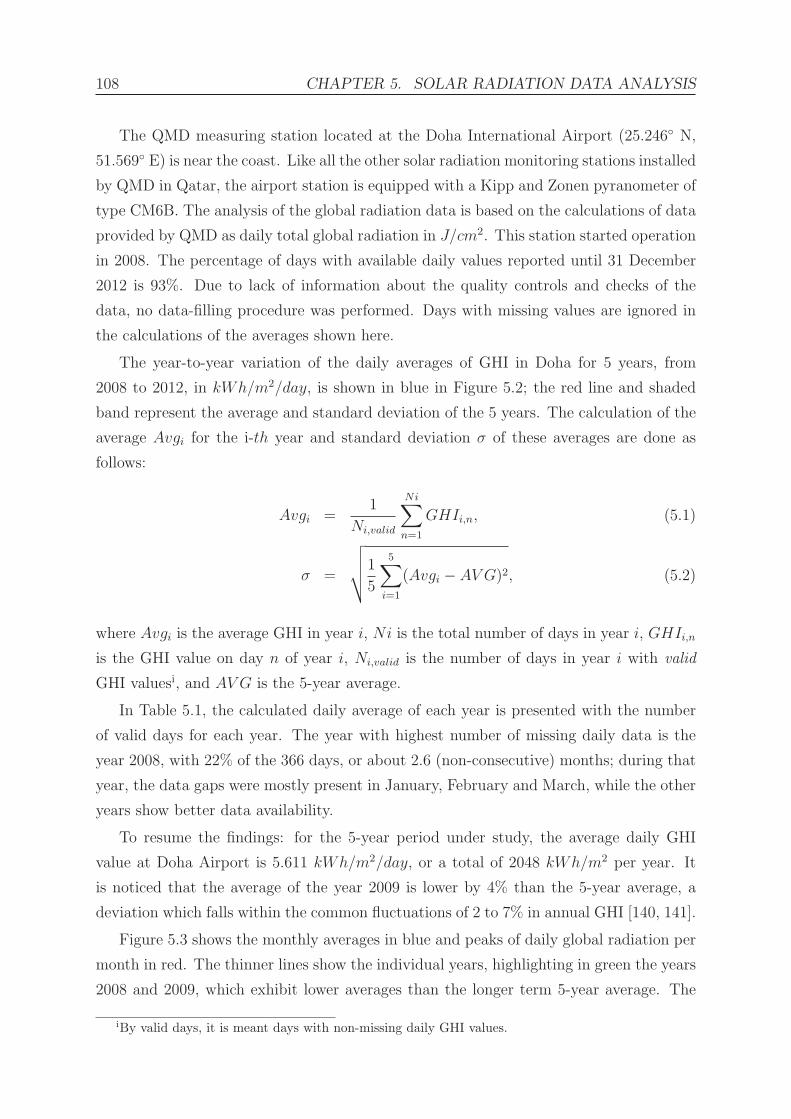
108 CHAPTER 5. SOLAR RADIATION DATA ANALYSIS
The QMD measuring station located at the Doha International Airport (25.246◦ N,
51.569◦ E) is near the coast. Like all the other solar radiation monitoring stations installed
by QMD in Qatar, the airport station is equipped with a Kipp and Zonen pyranometer of
type CM6B. The analysis of the global radiation data is based on the calculations of data
provided by QMD as daily total global radiation in J/cm2. This station started operation
in 2008. The percentage of days with available daily values reported until 31 December
2012 is 93%. Due to lack of information about the quality controls and checks of the
data, no data-filling procedure was performed. Days with missing values are ignored in
the calculations of the averages shown here.
The year-to-year variation of the daily averages of GHI in Doha for 5 years, from
2008 to 2012, in kWh/m2/day, is shown in blue in Figure 5.2; the red line and shaded
band represent the average and standard deviation of the 5 years. The calculation of the
average Avgi for the i-th year and standard deviation σ of these averages are done as
follows:
Avgi =1
Ni,valid
Ni∑n=1
GHIi,n, (5.1)
σ =
√√√√1
5
5∑i=1
(Avgi − AV G)2, (5.2)
where Avgi is the average GHI in year i, Ni is the total number of days in year i, GHIi,n
is the GHI value on day n of year i, Ni,valid is the number of days in year i with valid
GHI valuesi, and AV G is the 5-year average.
In Table 5.1, the calculated daily average of each year is presented with the number
of valid days for each year. The year with highest number of missing daily data is the
year 2008, with 22% of the 366 days, or about 2.6 (non-consecutive) months; during that
year, the data gaps were mostly present in January, February and March, while the other
years show better data availability.
To resume the findings: for the 5-year period under study, the average daily GHI
value at Doha Airport is 5.611 kWh/m2/day, or a total of 2048 kWh/m2 per year. It
is noticed that the average of the year 2009 is lower by 4% than the 5-year average, a
deviation which falls within the common fluctuations of 2 to 7% in annual GHI [140, 141].
Figure 5.3 shows the monthly averages in blue and peaks of daily global radiation per
month in red. The thinner lines show the individual years, highlighting in green the years
2008 and 2009, which exhibit lower averages than the longer term 5-year average. The
iBy valid days, it is meant days with non-missing daily GHI values.

5.1. QMD AUTOMATIC WEATHER STATIONS 109
Year Daily GHI [kWh/m2] Valid days
2008 5.675 286
2009 5.377 324
2010 5.735 360
2011 5.679 353
2012 5.579 348
Table 5.1: Annual means of daily GHI for Doha International Airport, and the corre-
sponding number of days with non-missing daily GHI values.
Year2008 2009 2010 2011 2012
/day
]2
GH
I [kw
h/m
5
5.1
5.2
5.3
5.4
5.5
5.6
5.7
5.8
5.9
6
Daily averages for one year period
Daily average for 5 years period
for 5 years periodσ
Figure 5.2: Annual variation of daily GHI averages at Doha International Airport.
average for the i-th month of the year was calculated as follows:
Avgi =
∑daysi
∑yrs
GHIi,yrs
Ni,valid
, (5.3)
which is the sum of the GHI values in month i for the 5 years, divided by Ni,valid, the
total number of days with valid values in month i during the 5-year period.
The figure shows that the monthly averages of GHI are above 6 kWh/m2/day from
April to September. Considering the whole year, the range goes from 4 to 7 kWh/m2/day.
The highest average is 6.967 kWh/m2/day, found in June, and the lowest is 3.867
kWh/m2/day, found in December. The highest peak is 8.411 kWh/m2/day, in June,
and the lowest peak is 4.77 kWh/m2/day, in December. As seen in Figure 5.2, the year
2009 exhibits a low yearly average compared to other years. In order to understand the
month by month contribution to the yearly average of the year 2009, this year is high-
lighted with a solid green line in Figure 5.3. The averages in July, August, and December
have lower values. In August 2009 there are only 6 days of valid daily data; although the

110 CHAPTER 5. SOLAR RADIATION DATA ANALYSIS
MonthJan Feb Mar Apr May Jun Jul Aug Sep Oct Nov Dec
/day
]2
GH
I [kW
h/m
0
1
2
3
4
5
6
7
8
9
10
Monthly averagesMaximum of daily values2010, 2011, 201220082009
Figure 5.3: Monthly averages and peaks of global radiation at Doha Airport throughout
the year.
calculated monthly average only considers the days with non-missing values, the average
obtained with these 6 days is not necessarily representative of the whole month. Similarly,
the year 2008 (green dashed line) also shows low values in the months of July, August,
and January, but the low values are compensated by higher values during the rest of the
months.
The daily averages of global radiation for the period from 2008 to 2012 in kWh/m2/day
are shown in Figure 5.4. The average for the i-th day of the year was calculated as follows:
Avgi =
Ny∑n=1
GHIi,n
Nyi,valid, (5.4)
where Ny = 5 is the total number of years and Nyi,valid is the number of years in which
day i has valid GHI values.
Similarly to the monthly averages, the daily averages have higher values during sum-
mer months. The highest daily average for the period 2008 to 2012 occurs during the
month of May and is 7.49 kWh/m2/day, while the lowest average is 3.02 kWh/m2/day,
in the month of November. The individual maximum daily values for each month are
shown in red in Figure 5.3.
To give more insight about solar radiation at the site, the clearness index was also
analysed. This index indicates the atmosphere’s effect on the transmission of solar ra-
diation. The monthly average clearness index K is defined [16] as the ratio of monthly
average of daily GHI to the monthly average, H0, of daily extraterrestrial radiation on a

5.1. QMD AUTOMATIC WEATHER STATIONS 111
Day of year50 100 150 200 250 300 350
/day
]2
GH
I [kW
h/m
0
1
2
3
4
5
6
7
8
Figure 5.4: Daily averages of global radiation at Doha Airport throughout the year.
horizontal plane (H0 from Equation 5.6), i.e.,
K =GHI
H0
(5.5)
In Figure 5.5, the monthly averages of the clearness index at Doha Airport are shown
for the period from 2008 to 2012, with their standard deviations. It is noticed that the
averaged K ranges from 0.58 to 0.65 and shows relatively small variations throughout
the year. This is due to a balance between cloudy days in the winter and hazy and dusty
days in the summer. Considering these more or less constant atmospheric conditions
between seasons, H0 and GHI change in parallel through the year (cf. Figures 5.11 and
5.4), and the monthly averages of K are relatively stable during a year period. It is also
seen that the standard deviations vary from month to month, depending on the stability
of the atmospheric conditions during each particular month.
On the same graph, the monthly K values obtained from the NASA-SSE database
are also shown. This database consists of monthly data, average of 22 years of satellite
measurements, from 1983 to 2005, provided for 1◦ × 1◦ pixels. The averages of K as
obtained by NASA range from 0.50 to 0.65, showing larger variations in a year period,
in comparison with the ground-based K. Between April and September, both graphs
are in good agreement. However, during the winter months from October to March the
NASA-SSE values are lower. It must be noted that the NASA-SSE values are longer-term
averages (22-year averages, from 1983 to 2005), while the ground values are derived from
a 5-year period (2008 to 2012), lying outside the coverage period of NASA-SSE. Given
that NASA-SSE values are modelled data, deviations from ground values are expected
depending on the validity of the model in the conditions of the region. Moreover, the
NASA-SSE value is the average over a region of 1◦×1◦. This translates to approximately
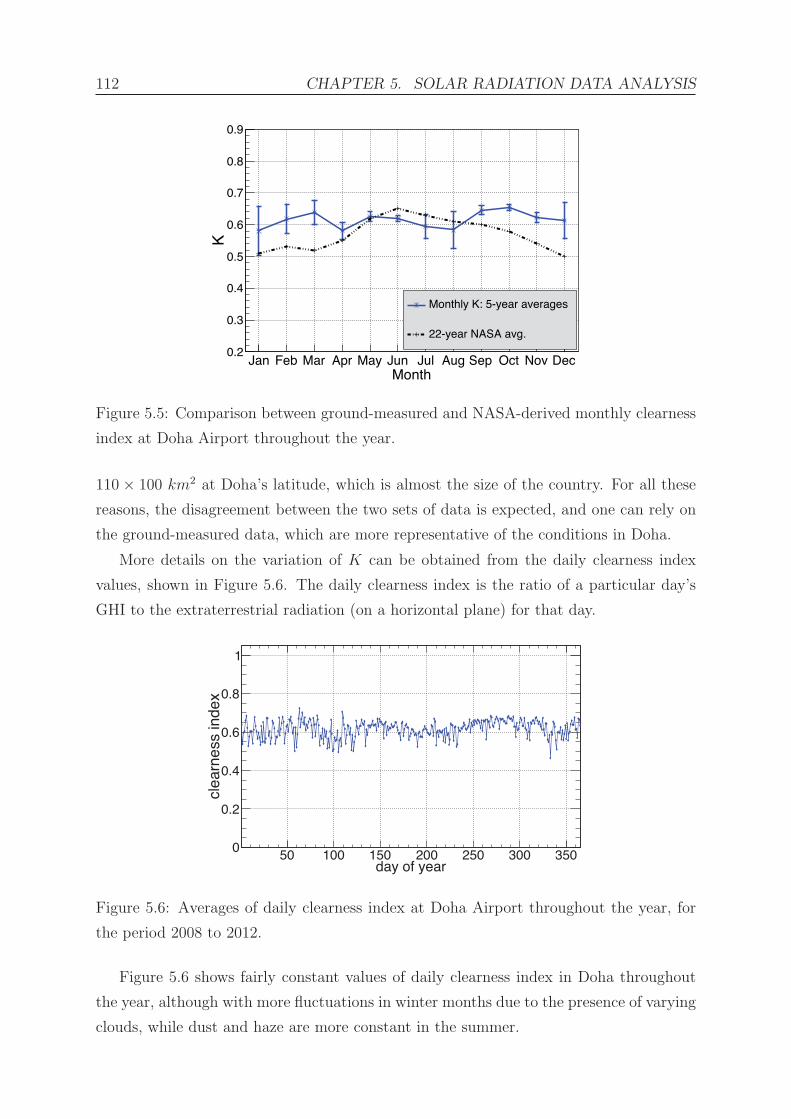
112 CHAPTER 5. SOLAR RADIATION DATA ANALYSIS
MonthJan Feb Mar Apr May Jun Jul Aug Sep Oct Nov Dec
K
0.2
0.3
0.4
0.5
0.6
0.7
0.8
0.9
Monthly K: 5-year averages
22-year NASA avg.
Figure 5.5: Comparison between ground-measured and NASA-derived monthly clearness
index at Doha Airport throughout the year.
110 × 100 km2 at Doha’s latitude, which is almost the size of the country. For all these
reasons, the disagreement between the two sets of data is expected, and one can rely on
the ground-measured data, which are more representative of the conditions in Doha.
More details on the variation of K can be obtained from the daily clearness index
values, shown in Figure 5.6. The daily clearness index is the ratio of a particular day’s
GHI to the extraterrestrial radiation (on a horizontal plane) for that day.
day of year50 100 150 200 250 300 350
clea
rnes
s in
dex
0
0.2
0.4
0.6
0.8
1
Figure 5.6: Averages of daily clearness index at Doha Airport throughout the year, for
the period 2008 to 2012.
Figure 5.6 shows fairly constant values of daily clearness index in Doha throughout
the year, although with more fluctuations in winter months due to the presence of varying
clouds, while dust and haze are more constant in the summer.

5.2. SOLAR RADIATION DATA ANALYSIS 113
The relation between sky conditions and daily values of clearness index has been
studied by [142, 143] for example, but there is no consensus on sky condition classifications
related to clearness index values. According to the European Solar Radiation Atlas
report [144], the 5-year average of K = 0.62 found in Doha implies very sunny climatic
conditions.
To have a point of reference and comparison with other values, Table 5.2 shows the
annual averages of the monthly K for Doha and other cities in the world. The 5-year
ground measurement-derived K for Doha is higher than the NASA-SSE value, while
ground measurements for Abu Dhabi [145] (1-year average) are lower than the NASA
value. Also included in the table are the year by year K values for Doha. As expected
from the GHI yearly averages, year 2009 shows a lower K than other years.
City K year by year (2008 to 2012)
Doha, grounda 0.62 0.61, 0.60, 0.63, 0.62, 0.62
Dohab 0.57
Abu Dhabi, groundc 0.58
Abu Dhabib 0.60
Ankarab 0.53
Cairob 0.60
Dammamb 0.61
Athensb 0.53
Tunisb 0.58
Tehranb 0.57
Table 5.2: Annual averages of clearness index for Doha and other cities; (a) 5-year average
of ground measurements, and year by year, (b) 22-year averages by NASSA-SSE, and (c)
1-year ground measurements, 2007.
5.2 Solar radiation data analysis
In this section, the analysis of ground measurements of solar radiation collected at the
QEERI site, 25.33◦N, 51.43◦E, is presented. The data was collected over one full year
starting from the 1st of December, 2012, to the 30th of November, 2013. By the nature of
the solar sensors used, the collected data are classified as DNI, GHI, and DHI (see Chapter
4 for more details on the experimental site and instruments). The three components
were collected as 1-minute average irradiances (averages of samples taken every second).
Considering no missing points in the data set, the total number of data per radiation

114 CHAPTER 5. SOLAR RADIATION DATA ANALYSIS
component for the year under study should be 525600 values. However, the actual total
number of collected values per component was 514763 data points, which means that the
data set has missing values equivalent to 7 days, 12 hours, 37 minutes, or 2% of the total.
The missing values were distributed as follows: 4 minutes missing in December 2012, 7
minutes missing in February 2013, and 10826 consecutive minutes missing in April 2013.
The missing data in April was due to a problem of the memory in the data logger. To
avoid similar problems in the future, an external memory card was fitted to the data
logger and is used as a backup for data recording. The missing data were ignored and no
data gap filling procedure was implemented. Instead, the averages were calculated based
on the actual collected data points.
5.2.1 Data quality control
Prior to any further data processing and analysis, quality control (QC) checks were per-
formed on the recorded data, following the BSRN standards [137], as discussed in Section
4.2.6. The procedure consists of flagging the 1-minute data of each component according
to checks on physical limits, extremely rare values and consistency tests among all com-
ponents (see formulas in Tables 4.5 and 4.6). All data with flags indicating failed tests
(from here on, called flagged data) detected by the QC procedure were then scrutinised
in order to understand the reasons behind the erroneous values. The data analyses in
the next sections are based on the data which passed the QC tests. Flagged data were
ignored and not considered in the calculation of the averages shown in this chapter.
For the used data set, Table 5.3 summarises the number of flagged 1-minute data (the
entries that failed the corresponding QC test) for the physically possible limits and the
extremely rare limits, per irradiance component (DNI, GHI and DHI) and per test. Table
5.4 shows the number of entries which failed the comparison tests: consistency among
the three components and the diffuse ratio test. Only data between sunrise and sunset
were considered in these tables; sunrise and sunset are determined by a solar zenith angle
of 90.83◦ according to the definition given by [146]; in order to check whether the data
that fail the QC checks are close to the sunrise or sunset times, statistics of data points
excluding moments close to sunrise and sunset are also shown: data with zenith angles
less than 85◦, 80◦ and 75◦. Figures 5.7 and 5.8 show the sunrise and sunset times for this
location in Doha through the year.
As a result of the quality control tests applied on the data set, the total number of
flagged data, about 1%, is negligible relatively to the total number of available data. For
the physical and extremely rare limits tests, the percentages of flagged data are greatly
reduced when excluding data close to the sunrise and sunset times, as expected because

5.2. SOLAR RADIATION DATA ANALYSIS 115
DateJan Feb Mar Apr May Jun Jul Aug Sep Oct Nov Dec Jan
Tim
e
04:45
05:00
05:15
05:30
05:45
06:00
06:15
Figure 5.7: Sunrise time calculated day by day over a period of one year at the QEERI
site in Doha, Qatar.
DateJan Feb Mar Apr May Jun Jul Aug Sep Oct Nov Dec Jan
Tim
e
16:45
17:00
17:15
17:30
17:45
18:00
18:15
18:30
Figure 5.8: Sunset time calculated day by day over a period of one year at the QEERI
site in Doha, Qatar.
of the lower performance of the sensors (pyranometers in particular) at low solar elevation
angles. For the comparison tests, the flagged data were checked against the log book as
discussed in Section 4.2.6, and it was found that for most of these flagged minutes, the
reason was an intervention or activity such as the routine cleaning of the sensor domes.
An additional check was used as a quick test to verify the consistency of the data
timestamps with respect to the sun’s position through the year. For this test, the complete
data sets, containing the values of DNI and GHI, collected as 1-minute averages over the
year of 2013, are presented in Figure 5.9, in a way to show the 365 days of the year on
the x-axis, and the 1440 minutes of each day on the y-axis, with a colour scale displaying
the radiation level at each point. The colour-coded intensity axis is on the right of each
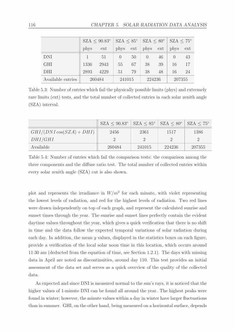
116 CHAPTER 5. SOLAR RADIATION DATA ANALYSIS
SZA ≤ 90.83◦ SZA ≤ 85◦ SZA ≤ 80◦ SZA ≤ 75◦
phys ext phys ext phys ext phys ext
DNI 1 51 0 50 0 46 0 43
GHI 1336 2943 55 67 38 39 16 17
DHI 2893 4229 51 79 38 48 16 24
Available entries 260484 241015 224236 207355
Table 5.3: Number of entries which fail the physically possible limits (phys) and extremely
rare limits (ext) tests, and the total number of collected entries in each solar zenith angle
(SZA) interval.
SZA ≤ 90.83◦ SZA ≤ 85◦ SZA ≤ 80◦ SZA ≤ 75◦
GHI/(DNI cos(SZA) +DHI) 2456 2361 1517 1386
DHI/GHI 2 2 2 2
Available 260484 241015 224236 207355
Table 5.4: Number of entries which fail the comparison tests: the comparison among the
three components and the diffuse ratio test. The total number of collected entries within
every solar zenith angle (SZA) cut is also shown.
plot and represents the irradiance in W/m2 for each minute, with violet representing
the lowest levels of radiation, and red for the highest levels of radiation. Two red lines
were drawn independently on top of each graph, and represent the calculated sunrise and
sunset times through the year. The sunrise and sunset lines perfectly contain the evident
daytime values throughout the year, which gives a quick verification that there is no shift
in time and the data follow the expected temporal variations of solar radiation during
each day. In addition, the mean y values, displayed in the statistics boxes on each figure,
provide a verification of the local solar noon time in this location, which occurs around
11:30 am (deducted from the equation of time, see Section 1.2.1). The days with missing
data in April are noted as discontinuities, around day 110. This test provides an initial
assessment of the data set and serves as a quick overview of the quality of the collected
data.
As expected and since DNI is measured normal to the sun’s rays, it is noticed that the
higher values of 1-minute DNI can be found all around the year. The highest peaks were
found in winter; however, the minute values within a day in winter have larger fluctuations
than in summer. GHI, on the other hand, being measured on a horizontal surface, depends

5.2. SOLAR RADIATION DATA ANALYSIS 117
Day of the year50 100 150 200 250 300 350
Min
ute
of th
e da
y
200
400
600
800
1000
1200
1400
0
200
400
600
800
1000
1200Mean x = 188.9Mean y = 692.9DNI
Day of the year50 100 150 200 250 300 350
Min
ute
of th
e da
y
200
400
600
800
1000
1200
1400
0
200
400
600
800
1000
1200Mean x = 182.2Mean y = 692.6GHI
Figure 5.9: 1-minute values of solar irradiance, in W/m2, through one year in Doha.
on the sun angles during the year and thus it is season-driven; the displayed minute values
of GHI show a smoother distribution through the year, with higher values concentrated
in the summer season. These behaviours are furtherly analysed in the following sections,
by aggregating the data in terms of hourly, daily and monthly averages.
Data gap filling
In general, in Geosciences, several approaches can be applied in order to fill the gaps
found in the data sets. These methods are either parametric (based on models) or non-
parametric (depending only on the data) [147, 148, 149, 150]. In solar radiation, similar
procedures could be implemented for filling the gaps. The length of the gap, i.e., hourly
data missing in one day, or daily data missing in a year, etc. is one of the main factors to
take into account when deciding on the data gap filling method. For instance, the National
Solar Radiation Database (NSRDB) of the USA, uses the following methods for filling
the gaps in the data set of measurements, taken between 1961 and 1990: for gaps of 5

118 CHAPTER 5. SOLAR RADIATION DATA ANALYSIS
hours or less, linear interpolation is used, for gaps from 6 to 47 hours, they substitute data
from the same hours of adjacent days, and for gaps of 2 days to one year, the substitution
of data is from the same calendar days from another similar year [151]. They have also
investigated other methods such as filling the solar model input parameters and modelling
the solar irradiance based on the filled input parameters. They also used modelled data
for filling gaps in the measured data. Gap filling procedures for solar radiation data were
also developed as part of the Solar Radiation Resource Assessment (SRRA) project in
India, which describes the Indian experience in operating solar monitoring stations [152].
Their basic gap filling procedure relies on the availability of the three components of solar
radiation (DNI, GHI and DHI) and on the duration of the gap, with gaps up to 3 hours,
greater than 3 hours and gaps greater than 24 hours, and consist of using the equation
relating the three components, modelled values, linear interpolation of clearness indices
or by replacing data from neighbouring days. The standardisation of procedures for gap
filling is also in the core activity of the IEA Task 46 “Solar Resource Assessment and
Forecasting”, which addresses the basic objectives and means to understand and improve
the knowledge of solar energy resources [64].
In this thesis work, the missing values are due to two reasons: either the value was
recorded but flagged by the quality control tests and therefore considered as missing, or
the value was not recorded by the data acquisition system. As commented before, it was
decided not to apply any gap filling for this work, so the averages represent the available
minutes. The number of missing minutes in December and February was negligible, so
they have no effect on the calculation of the averages; in April, although the number of
missing minutes is not negligible, the decision of ignoring these days in the calculation of
the averages was based on the fact that several years of measurements should be available
in order to decide on and apply a procedure for filling the gaps, in particular when several
days are missing, and such data is currently not available for Doha, or any part of Qatar.
5.2.2 Extraterrestrial solar radiation
As seen in Chapter 1, the radiation emitted by the sun and arriving at the top of the
earth’s atmosphere, known as the extraterrestrial radiation, is not constant through the
year, changing by ±3.3% depending on the distance between the earth and the sun.
Figure 5.10 shows how the extraterrestrial radiation varies throughout a year, because
of the changes in the sun-earth distance. Equation 1.1 is used for the calculation of the
direct, or beam, extraterrestrial radiation calculated on a plane perpendicular to the sun’s
rays at the top of the earth’s atmosphere.
The extraterrestrial radiation on a horizontal surface (also at the top of the atmo-

5.2. SOLAR RADIATION DATA ANALYSIS 119
Date01/01 01/02 01/03 01/04 01/05 01/06 01/07 01/08 01/09 01/10 01/11 01/12 01/01
]2E
T [W
/m
1320
1340
1360
1380
1400
Figure 5.10: Variation of the beam extraterrestrial solar irradiance in a one-year period.
sphere) depends, in addition, on the position of the sun relative to the location on the
earth’s surface. At any time, it can be calculated from the direct extraterrestrial radia-
tion modulated by cos θz, the cosine of the zenith angle of the sun (θz) at that time, and
can be integrated over the period from sunrise to sunset in order to obtain the total daily
extraterrestrial radiation on a horizontal surface, denoted as H0. The term cos θz, given
by Equation 1.3, takes into account the geometry and the position of the horizontal sur-
face with reference to the angle of incidence of the solar radiation, that is, the declination
angle of the sun (δ), the latitude of the surface of interest (φ) and the solar hour angle
(h). H0 can be calculated, in W/m2, as follows [16]:
H0 = I0 ·[1 + 0.033 · cos
(2πn
365
)]· cos(θz), (5.6)
where I0 is the solar constant (1367 W/m2), n is the day of the year (1 to 365), and θz is
the zenith angle of the sun. For more information on the sun geometric angles, refer to
Section 1.2.1. Figure 5.11 shows the variation of the daily total extraterrestrial radiation
on a horizontal surface throughout the year, for the location of the experimental site.
It is clear that the variation of the daily extraterrestrial radiation at this location is
relatively large and the radiation is about 70% higher in summer than in winter. This is
a crucial feature and is used in the study of the atmosphere when it comes to calculating
the normalised level of radiation at ground level, that is, the amount of radiation at the
surface of the earth compared to the amount of radiation at the top of the atmosphere.

120 CHAPTER 5. SOLAR RADIATION DATA ANALYSIS
Date01/01 01/02 01/03 01/04 01/05 01/06 01/07 01/08 01/09 01/10 01/11 01/12 01/01
/day
]2
[kW
h/m
0H
6
7
8
9
10
11
Figure 5.11: Variation of the daily extraterrestrial solar irradiation on a horizontal surface
at the experimental site in Doha, in a one-year period.
5.2.3 Hourly, daily and monthly irradiances
An analysis of the ground-measured solar data at the location under study is given in
this section. The goal is to study the characteristics of solar radiation in Doha over a
one-year period, from December 2012 to November 2013.
The quality-controlled minute values of DNI, GHI and DHI inW/m2 were used for the
calculation of the hourly, daily and monthly averages. The month of April shows a gap
in the data but no gap filling procedures were used, as discussed in Section 5.2.1, so April
was represented by 23 days of data (around 77% of the month’s possible values). For the
calculation of the averages, only daytime (from sunrise to sunset) minute values which
pass the quality control tests of physical limits and consistency were included. Night
values, which are usually negative in the GHI and DHI signals due to the thermal offset
of pyranometers (see Section 1.3), were set to zero for the 3 components and counted
in the calculation of daily and monthly averages, i.e., these averages are normalised to
days of 24 hours. For the calculation of the hourly averages, all minute values within the
sunrise to sunset interval, regardless of their sign, were considered as long as they pass
the quality checks. Close to the sunrise and sunset hours, the measured values are close
to zero but both positive and negative values can be found. It was decided to include all
in the calculation of hourly averages (note that this only affects the hours including the
instants of sunrise and sunset) because of the measurement uncertainties.
The averages of hourly DNI, GHI and DHI are shown in Figure 5.12, considering
the whole year. The averages are calculated in 24 bins of 1 hour each. The bin 12, for
example, represents the average of the minutes from 11:01 am until 12:00 pm. The curves

5.2. SOLAR RADIATION DATA ANALYSIS 121
present a more or less symmetrical shape centred around solar noon, the typical variation
of the solar radiation during daytime, from sunrise to sunset. It is noticed in the graph,
that shortly after solar noon the direct radiation tends to be slightly lower than just
before solar noon. This is probably due to the stabilisation of the atmospheric conditions
in the afternoon period, concentrating a higher amount of aerosols in the atmosphere.
This is not the case of the global radiation, since the lower level of the direct component
is compensated by an increase of the diffuse component at that time.
Hour0 2 4 6 8 10 12 14 16 18 20 22 24
]2Ir
radi
ance
[W/m
0
100
200
300
400
500
600
700
800
900
DNI
GHI
DHI
Figure 5.12: Hourly DNI, GHI and DHI in Doha, averaged over one year, from December
2012 to November 2013.
Note also that, as shown in Figures 5.7 and 5.8, the sunrise and sunset times change
from day to day, and for the experimental site there is a maximum difference of around
1 hour and a half between winter and summer. For more clarity and in order to separate
the averages along the year, the hourly averages were calculated for each month and are
presented in Figure 5.13 for DNI, GHI and DHI. GHI hourly averages are higher in the
summer months, and for hours close to solar noon one can distinguish two periods: one
with higher level of radiation, including the months from March to October, and the
second with relatively lower level of radiation, from November to February. This is not
the same for the hourly averages of DNI, which do not exhibit a clear seasonal trend from
month to month; the month of October shows the highest DNI levels and April shows the
lowest levels of DNI during this year of data collection; although April was represented by
77% of its data points, little or no bias is expected to result from this and the calculated
averages are estimated to be representative, since hazy and dusty conditions were present
most of the days of this month, as the daily averages will indicate. Nevertheless, an
accurate estimation of the bias is only possible by comparing with a different set of
ground measurements of a nearby station, which is not available.
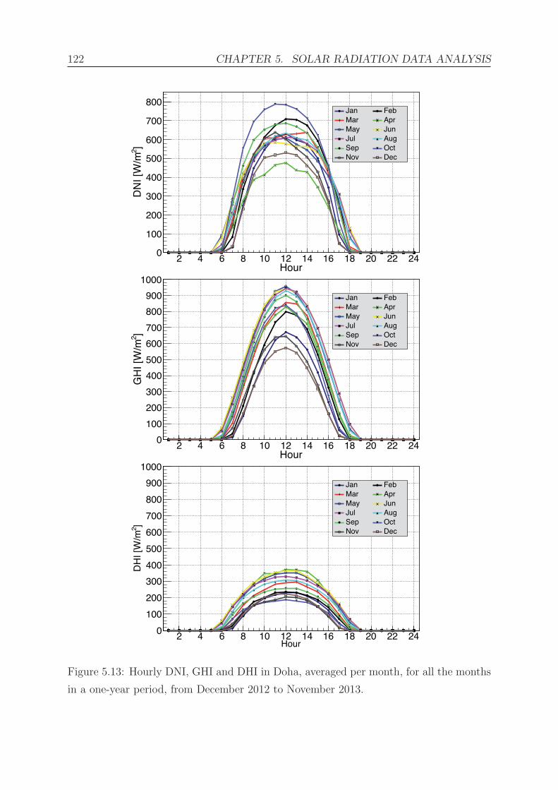
122 CHAPTER 5. SOLAR RADIATION DATA ANALYSIS
Hour2 4 6 8 10 12 14 16 18 20 22 24
]2D
NI [
W/m
0
100
200
300
400
500
600
700
800Jan FebMar AprMay JunJul AugSep OctNov Dec
Hour2 4 6 8 10 12 14 16 18 20 22 24
]2G
HI [
W/m
0
100
200
300
400
500
600
700
800
900
1000
Jan FebMar AprMay JunJul AugSep OctNov Dec
Hour2 4 6 8 10 12 14 16 18 20 22 24
]2D
HI [
W/m
0
100
200
300
400
500
600
700
800
900
1000
Jan FebMar AprMay JunJul AugSep OctNov Dec
Figure 5.13: Hourly DNI, GHI and DHI in Doha, averaged per month, for all the months
in a one-year period, from December 2012 to November 2013.

5.2. SOLAR RADIATION DATA ANALYSIS 123
The daily averages of DNI, GHI and DHI are shown in Figure 5.14. The maximum
1-minute value of the day is shown in red. As discussed, these averages include the 24
hours of the day. For clarity in the graphs, to help differentiate visually between missing
and actual low averages, missing days are shown as -50 W/m2 (7 days in total) and days
with more than 3.5 hours of missing data are shown as -60 W/m2 (1 day). In general, it
is noted that the daily values, and even the minute peaks, show larger fluctuations from
November (last days in the plots) to June (around day 210), due to the occasional and
intermittent cloudy conditions in these months, than from July to October, when days
are mostly cloudless but often with a presence of haze and dust for days or weeks at a
time.
The daily averages of DNI display large day to day fluctuations during this period with
no evident seasonal changes through the year. This is due to the different atmospheric
conditions encountered in the atmosphere of Doha from day to day, which can change
from clear to cloudy (mainly in winter), hazy or dusty (mainly in summer), anytime
during the year. The 1-minute peaks are in general higher during winter than in summer,
due to higher aerosol levels in the summer that continuously decrease the level of direct
radiation. The maximum daily average of DNI was calculated for 25 May with a value
of 407.2 W/m2, and the maximum measured minute DNI value was 987.5 W/m2, on 22
March 2013.
The daily GHI averages show smaller day to day fluctuations in general and, as
expected, values are higher during the summer months. The highest daily GHI average is
found on 30 May with a value of 356 W/m2 and the highest minute GHI value is 1231.5
W/m2, measured on the first of May 2013.
Daily DHI averages show relatively constant values until March, when values started
increasing because of more days with dust and haze, until around mid-August, when DHI
started decreasing again. The highest daily DHI average value is 205.8 W/m2, found in
the summer, on 11 June, and the maximum minute DHI value is recorded for the first of
May 2013, with the value of 757.7 W/m2.
The monthly averages of DNI, GHI and DHI are shown in blue in Figure 5.15 and
the maximum daily averages for each month are shown in red. The monthly averages are
calculated from the 1-minute values of radiation.
The monthly DNI averages increased from December to February and remained almost
constant from March until September, except for the low value observed in April. As
discussed before, the low average in April is estimated to effectively represent the radiation
level available during this month; while it is true that this month has missing values which
were not counted in the calculation of the monthly average, it is unlikely that these days

124 CHAPTER 5. SOLAR RADIATION DATA ANALYSIS
Day0 50 100 150 200 250 300 350
]2Ir
radi
ance
[W/m
0
200
400
600
800
1000
1200Average Maximum DNI
Day0 50 100 150 200 250 300 350
]2Ir
radi
ance
[W/m
0
200
400
600
800
1000
1200
Average Maximum
GHI
Day0 50 100 150 200 250 300 350
]2Ir
radi
ance
[W/m
0
200
400
600
800
1000
1200Average Maximum DHI
Figure 5.14: Daily averages and maximum minute values per day for DNI, GHI and DHI
in Doha in one year, from Dec/2012 to Nov/2013. Values for missing days are set to
negative (see text).
had high levels of radiation, because of the values seen around this period (cf. Figure 5.14)
and because during the month of April there was a high frequency of cloudy days and
days with dusty and/or hazy conditions, to which DNI is highly sensitive [5]. The month

5.2. SOLAR RADIATION DATA ANALYSIS 125
MonthDec Jan Feb Mar Apr May Jun Jul Aug Sep Oct Nov
]2Ir
radi
ance
[W/m
0
100
200
300
400
500Average Maximum DNI
MonthDec Jan Feb Mar Apr May Jun Jul Aug Sep Oct Nov
]2Ir
radi
ance
[W/m
0
100
200
300
400
500Average Maximum GHI
MonthDec Jan Feb Mar Apr May Jun Jul Aug Sep Oct Nov
]2Ir
radi
ance
[W/m
0
100
200
300
400
500Average Maximum DHI
Figure 5.15: Monthly averages and maximum daily values per month for DNI, GHI and
DHI in Doha during one year, from December 2012 to November 2013.
of October shows the highest average of DNI with a value of 275 W/m2. Atmospheric
conditions during this month were particularly clean and there were few days with dust
or haze.
The monthly averages of GHI have high values in summer time, except from March

126 CHAPTER 5. SOLAR RADIATION DATA ANALYSIS
to April where the value remains almost constant. From May to July, GHI monthly
averages are above 300 W/m2, with the highest monthly average of 315.5 W/m2 in June.
The lowest value was observed in December with 165 W/m2, which means that GHI
values almost doubled between December and June.
DHI monthly averages show higher values in the summer, with the highest in June
with 135.6 W/m2. The lowest monthly averages of 65 W/m2 were found in December
2012, October and November 2013.
The monthly averages of GHI calculated for the QEERI station were compared with
the longer-term (5 years, 2008–2012) monthly averages calculated in Section 5.1.1, for
the station at the Doha International Airport belonging to QMD. This is summarised in
Table 5.5. The relative difference between the two data sets is less than ±10% for all
months, which means that the current measurements are consistent with historical data
observed in Doha. The relative difference in April is less than ±1%, which indicates that
the low monthly average calculated for this month at the QEERI station is not biased
by the missing values.
Month QEERI QMD rDifference (%)
Dec 3.61 3.87 7.2
Jan 4.21 4.02 -4.5
Feb 5.24 4.80 -8.4
Mar 6.12 5.81 -5.1
Apr 6.02 6.05 0.5
May 7.28 6.92 -4.9
Jun 7.57 6.97 -7.9
Jul 7.36 6.65 -9.6
Aug 6.95 6.36 -8.5
Sep 6.47 6.17 -4.6
Oct 5.76 5.35 -7.1
Nov 4.18 4.30 2.9
Table 5.5: Comparison of monthly averages of GHI in Doha, in kWh/m2/day: based on
one year of data collected by the QEERI solar station and 5 years of data collected by
the QMD station.

5.2. SOLAR RADIATION DATA ANALYSIS 127
5.2.4 Frequency distributions
In addition to the aggregation of data in terms of hourly, daily and monthly averages, to
have a more complete characterisation of the solar radiation at the location under study it
is useful to present the frequency distribution of the data, specially since data are available
at high temporal resolution (1-minute values). These distributions are considered an
important statistical tool for the adaptation of modelled solar data to the measured
values and for the validation of prediction models [7]. They are also useful for site
selection, systems design and performance studies of solar energy plants [153]. Figure
5.16 shows the relative frequency distributions of minute DNI and GHI during daytime,
for the period under study. Each bin is of 50 W/m2, and each curve was normalised to
100%. The thin, coloured lines represent the frequencies in each month, and the added
distributions for the year are depicted by the thick line.
]2Irradiance [W/m200 400 600 800 1000 1200
Fre
quen
cy (
%)
0
5
10
15
20
25
30
35Dec Jan Feb Mar
Apr May Jun Jul
Aug Sep Oct Nov
All
DNI
]2Irradiance [W/m200 400 600 800 1000 1200
Fre
quen
cy (
%)
0
5
10
15
20
25
30
35Dec Jan Feb Mar
Apr May Jun Jul
Aug Sep Oct Nov
All
GHI
Figure 5.16: Frequency distributions of one-minute values of solar irradiance through one
year in Doha. All distributions are normalised to 100% for comparison clarity.
One can notice that moderate values of DNI are measured for this location, having
a frequency peak around 650 W/m2 and a wide dispersion. DNI occurrence appears

128 CHAPTER 5. SOLAR RADIATION DATA ANALYSIS
not to follow a clear seasonal variation when comparing consecutive months; however,
peaks of high radiation are more frequent in the winter season and peaks of lower level
of radiation are common during the months with dust and haze such as April, May and
June. In contrast, GHI has a clear seasonal variation; a frequency peak around 650 W/m2
is seen for October, November and December and the distributions do not exceed 800
W/m2; January and September are transition months towards higher radiation, and the
rest of the months have frequency peaks around 900 W/m2 with the radiation reaching
more than 1000 W/m2.
5.2.5 Atmospheric transmission
The atmospheric conditions play an important role in the variations of the solar radiation
in Doha during a period of a year. These variations are seen at the different averaging
levels shown previously, which give a broader view about how the radiation level is chang-
ing through the year from hour to hour, from day to day and from month to month. In
order to give more details about the state of the atmosphere, the clearness index Kt and
the diffuse ratio Kd were investigated. The clearness index is defined [16] as the ratio
of GHI to extraterrestrial radiation on the horizontal surface (H0). The diffuse ratio is
the ratio of DHI to GHI. These two indices give good indication about the transmission
of solar radiation in Doha’s atmospheric conditions characterised by high aerosol loads
most of the year, mainly due to desert dust and industrial emissions.
Figure 5.17 shows the monthly averages of clearness index and diffuse ratio in Doha
for the period under study.
MonthDec Jan Feb Mar Apr May Jun Jul Aug Sep Oct Nov
Val
ue
0
0.1
0.2
0.3
0.4
0.5
0.6
0.7
0.8
0.9
1Clearness index
Diffuse ratio
Figure 5.17: Monthly clearness index and diffuse ratio in Doha during one year, from
Dec/2012 to Nov/2013.
Kt averages range from 0.57 to 0.70. The clearness index averages from February to

5.2. SOLAR RADIATION DATA ANALYSIS 129
September are almost constant, except in April, as commented before; October had the
highest clearness index, due to the clean atmosphere observed in October, as seen in the
high level of DNI radiation in the monthly, daily and hourly averages. In contrast, Kd
shows larger variations, ranging from 0.27 to 0.52, with the lowest diffuse ratio in October.
As can be seen by comparing both graphs, these two indices are in general inversely
related, i.e., low diffuse ratios correspond to clearer skies, and vice versa. This relationship
is an essential feature in the modelling of solar radiation and has been extensively studied
in the literature for the derivation of the solar radiation components.
Daily averages of both indices are shown in Figure 5.18. They show the same be-
haviour as the monthly averages, but with bigger fluctuations due to the higher resolution
of the daily averages, with more details being smoothed in the monthly averages. The
daily clearness index is also generally stable but shows some large drops which lower the
monthly averages in December, April and November. The yearly averages ofKt andKd in
this period are 0.65 and 0.39, respectively. These values imply a generally sunny climate
but with high levels of sunlight diffusion because of dust and aerosols in the atmosphere.

130 CHAPTER 5. SOLAR RADIATION DATA ANALYSIS
Day0 50 100 150 200 250 300 350
Cle
arne
ss in
dex
0
0.1
0.2
0.3
0.4
0.5
0.6
0.7
0.8
0.9
1
Day0 50 100 150 200 250 300 350
Diff
use
ratio
0
0.1
0.2
0.3
0.4
0.5
0.6
0.7
0.8
0.9
1
Figure 5.18: Daily clearness index and diffuse ratio in Doha during one year, from
Dec/2012 to Nov/2013.
Chapter 6
Correlation of DNI with backscatter
This chapter is dedicated to the study of the lidar backscatter signals. This includes in
particular the study of the noise imbedded in the signals measured by the lidar. The
noise analysis was done to find a limit on the atmospheric height used for the integration
of the lidar signal. The second part of the chapter, the ultimate goal of this thesis work,
describes the methodology correlating the lidar backscatter profiles with solar radiation.
A validation of the results is done through the use of solar data derived from two known
satellite databases, acquired for the same location and time. Through the derived model,
this study shows how aerosol data as assessed by the backscatter signal of a lidar ceilome-
ter can provide relevant information about the state of the atmosphere in Doha. This
information is directly related to the amount and quality of solar radiation available at
ground level, in particular a decreased level of the direct radiation and an increased level
of the diffuse radiation. Therefore, it can be deducted that aerosol information extracted
from lidar measurements can be used as an alternative input for solar radiation modelling
or for the calibration of satellite-derived solar data.
6.1 Ceilometer signal analysis
As described in Chapter 4, the signal processing by the data acquisition system of the
CL51 ceilometer is performed in real time and consists of acquiring the backscatter signal,
applying the range correction, subtracting the noise, calculating the first three cloud base
heights or the vertical visibility from the attenuated backscatter signal, and displaying
the results in terms of range-corrected (i.e., multiplied by the corresponding height)
backscatter profiles or cloud height profiles. The raw data for the present study are the
range-corrected backscatter coefficients recorded each 36 s with 10 m resolution, and
a maximum height of 15 km. The study was limited to the clear days of the year, in
131

132 CHAPTER 6. CORRELATION OF DNI WITH BACKSCATTER
order to avoid wrong information that may arise, in the averaging or data analysis of the
backscatter coefficients, from the presence of a cloud. A detailed explanation of the ‘clear
days’ selection is given in Section 6.2.1.
In addition, the integration of the backscatter coefficients in the vertical column was
limited to 5 km. This limit was found to be a good compromise between including the
required information for the analysis and excluding the noise-dominated signal provided
by the ceilometer during a period of one year. The selection of 5 km is the result of
different analyses in a detailed study of the ceilometer signal, presented in the following
subsections.
The ceilometer signal performance decreases with increasing altitudes and a noisier
profile at higher altitudes is observed in the ceilometer measurements, as can be seen
in Figure 6.1. This figure shows the variation of the hourly-averaged backscatter coeffi-
cients at solar noon (the hour from 11:00:01 am to 12:00:00 pm) versus the height in the
atmosphere up to 10 km, for all the clear days during a period of one year. Each line
represents the hourly backscatter coefficients of one day, and the height shown is limited
to 10 km for visual clarity. This figure is similar to, but not the same as, the right-hand
side graph in Figure 4.6. Pronounced aerosol layers can be distinguished at low altitudes
as large, positive signals, and a noisier signal is seen at high altitudes as highly variable
signals, randomly oscillating between negative and positive amplitudes. The main prob-
lem affecting the ceilometer signal around noon is the background noise from the sun,
mainly during summer, when the sun is almost directly overhead and within the line of
view of the lidar.
Height [km]0 2 4 6 8 10
-1*s
rad*
km]
5B
acks
catte
r [1
0
-4000
-3000
-2000
-1000
0
1000
2000
3000
4000
5000
Figure 6.1: Variation of the hourly-averaged backscatter coefficients with height, at solar
noon, for all the clear days through one year in Doha.
Several tests, presented in Sections 6.1.1 to 6.1.3, have been carried out to understand

6.1. CEILOMETER SIGNAL ANALYSIS 133
the behaviour of the signal as a function of the height and from one day to another. This
allows to understand the signal to noise ratio and to determine the maximum height in
the atmosphere where the lidar signal has less level of noise. These tests include the
study of the cumulative distribution, the average, the standard deviation, the frequency
distribution, and the variability of the range of the hourly backscattered coefficients in
binned heights. The objective was to obtain qualitative information about the nature and
behaviour of the lidar signal in each bin of height and identify a height after which any
real signals cannot be distinguished or separated from noise (in cloud-free conditions).
The tests were applied for each of the months of the year separately except for the last
test in Section 6.1.3, which includes all the clear days together. This allows to spot any
month or season dependency in the studied signal and to rely on the test which applies
for all months, without any dependency on season or atmospheric contents. The hourly
averages of the backscatter coefficient, hereby called beta coefficients, were obtained from
the 36-s backscatter coefficients with height steps of 10 m, up to 15 km. In the plots
shown in the following sections, the data were averaged in bins of 500 m. Several bin
widths were tested and 500 m was found to be a good compromise between smoothing
out the high resolution oscillations and keeping a good representativeness of the beta
values for the analysis.
6.1.1 Cumulative beta
For each clear day, the hourly-averaged beta values, measured at noon, were grouped in
bins of 500 m in height. The cumulative beta plots, shown in Figure 6.2, are presented
as one line per day.
By studying the cumulative beta, it is expected to have the beta accumulation of the
hourly coefficients increasing with height, until a certain height, at which the cumulative
beta value becomes constant or very slowly-varying. This is because real signals are
positive, and if after some height the signal becomes dominated by noise, the added
signals should cancel by their alternating negative and positive amplitudes (see Figure
6.1).
As one can see, the cumulative beta in the plots stabilises at different heights de-
pending on the month. This shows that the height where the cumulative beta reaches
a stable value, is season- and month-dependent. It is also noted that cumulative beta
starts to decrease after the so-defined stabilisation height. The dominance of negative
values at high altitudes is most likely due to the noise cancellation method adopted by
Vaisala. This method seems not to work effectively for all seasons under the conditions
of this experiment. Indeed, the ceilometer’s tilt option, meant to avoid the direct sun

134 CHAPTER 6. CORRELATION OF DNI WITH BACKSCATTER
Height [km]0 2 4 6 8 10 12 14
-1*s
rad*
km]
5B
eta
[10
0
20
40
60
80
100
120310×
12/2012
Height [km]0 2 4 6 8 10 12 14
-1*s
rad*
km]
5B
eta
[10
0
20
40
60
80
100
310×
01/2013
Height [km]0 2 4 6 8 10 12 14
-1*s
rad*
km]
5B
eta
[10
0
20
40
60
80
100
120
140
310×
02/2013
Height [km]0 2 4 6 8 10 12 14
-1*s
rad*
km]
5B
eta
[10
0
20
40
60
80
100
120
140310×
03/2013
Height [km]0 2 4 6 8 10 12 14
-1*s
rad*
km]
5B
eta
[10
020406080
100120140160180
310×
04/2013
Height [km]0 2 4 6 8 10 12 14
-1*s
rad*
km]
5B
eta
[10
-40-20
020406080
100120140
310×
05/2013
Height [km]0 2 4 6 8 10 12 14
-1*s
rad*
km]
5B
eta
[10
-200
-150
-100
-50
0
50
100
150
200310×
06/2013
Height [km]0 2 4 6 8 10 12 14
-1*s
rad*
km]
5B
eta
[10
-50
0
50
100
150
310×
07/2013
Height [km]0 2 4 6 8 10 12 14
-1*s
rad*
km]
5B
eta
[10
020406080
100120140160180200
310×
08/2013
Height [km]0 2 4 6 8 10 12 14
-1*s
rad*
km]
5B
eta
[10
020406080
100120140160180
310×
09/2013
Height [km]0 2 4 6 8 10 12 14
-1*s
rad*
km]
5B
eta
[10
0
20
40
60
80
100
120
140
310×
10/2013
Height [km]0 2 4 6 8 10 12 14
-1*s
rad*
km]
5B
eta
[10
0
20
40
60
80
100310×
11/2013
Figure 6.2: Cumulative beta in 500-m steps, at solar noon for the clear days of all the
months of the year under study.

6.1. CEILOMETER SIGNAL ANALYSIS 135
rays, was not used in the current setup of this experiment and the device was kept in
its vertical position all through the year. Therefore, the background noise from the sun
is sometimes affecting the lidar signal. With these conditions, the background noise is
more pronounced in summer than in winter, since the position of the sun in the sky is
very close to the line of view of the ceilometer in summer. Probably, this effect is not
properly taken into account in the noise cancellation process. It should be noted that
the information given by Vaisala regarding background noise cancellation is very brief
and does not provide a precise understanding of the method. Another important feature
seen in these plots is the abrupt increase of the cumulative beta at low heights, followed
by a slower increase up to the stabilisation height. This is due to the highly changing
constituents in terms of concentrations and species type between the different layers in
the first few km of the atmosphere. The change continues with height, but with a slower
rate due to the mixing happening on the way up to the top of the boundary layer, where
the mixing is almost complete. The current test was useful to detect a month-dependent
height from which the effect of the noise starts to affect the signal. However, and in order
to have a unified height selection independent of the month, other tests were conducted,
as described in the next subsections.
6.1.2 Day-to-day variability of beta
The constituents of the atmosphere within the range of the ceilometer change on daily
basis. In order to understand up to which height in the atmosphere these changes are still
discernible with the CL51, the average of the backscatter coefficients was calculated at
each height for all the clear days of each month and month by month, then the values were
averaged in bins of 500 m and plotted versus the height. This is useful to compare how,
on average, the atmospheric conditions change between subsequent height bins in the
atmosphere, as seen in Figure 6.3. It is expected that the average backscatter coefficients
at heights where the noise is dominant should show lower values (close to zero) than
those of real signals, due to the positive and negative amplitudes of noise. The figure
shows that the average backscatter coefficient decreases rapidly as height increases, then
remains roughly constant up to a certain height, and decreases again at higher altitudes.
However, at even higher altitudes the signal deviates from zero, which indicates that at
the highest altitudes the negative and positive values are not cancelling out.
What can be distinguished in these graphs, are the large variations of the average
backscatter coefficient from one height bin to another in the first 4 to 5 km in comparison
to the variations after these heights, and this is found in all the months. This gives
indication that the observed atmospheric conditions after 4 to 5 km, as profiled by the

136 CHAPTER 6. CORRELATION OF DNI WITH BACKSCATTER
Height [km]0 2 4 6 8 10 12 14 16
-1*s
rad*
km]
5B
eta
aver
age
[10
-50
0
50
100
150
200
250
300
12/2012
Height [km]0 2 4 6 8 10 12 14 16
-1*s
rad*
km]
5B
eta
aver
age
[10
-100-50
050
100150200250300350
01/2013
Height [km]0 2 4 6 8 10 12 14 16
-1*s
rad*
km]
5B
eta
aver
age
[10
-100-50
050
100150200250300
02/2013
Height [km]0 2 4 6 8 10 12 14 16
-1*s
rad*
km]
5B
eta
aver
age
[10
-100-50
050
100150200250300350
03/2013
Height [km]0 2 4 6 8 10 12 14 16
-1*s
rad*
km]
5B
eta
aver
age
[10
-100
0
100
200
300
400
500
04/2013
Height [km]0 2 4 6 8 10 12 14 16
-1*s
rad*
km]
5B
eta
aver
age
[10
-200
-100
0
100
200
300
40005/2013
Height [km]0 2 4 6 8 10 12 14 16
-1*s
rad*
km]
5B
eta
aver
age
[10
-200
0
200
400
600
800
06/2013
Height [km]0 2 4 6 8 10 12 14 16
-1*s
rad*
km]
5B
eta
aver
age
[10
-100
0
100
200
300
400
07/2013
Height [km]0 2 4 6 8 10 12 14 16
-1*s
rad*
km]
5B
eta
aver
age
[10
-100
0
100
200
300 08/2013
Height [km]0 2 4 6 8 10 12 14 16
-1*s
rad*
km]
5B
eta
aver
age
[10
-100
0
100
200
300
400
09/2013
Height [km]0 2 4 6 8 10 12 14 16
-1*s
rad*
km]
5B
eta
aver
age
[10
-100
-50
0
50
100
150
200
250
300
10/2013
Height [km]0 2 4 6 8 10 12 14 16
-1*s
rad*
km]
5B
eta
aver
age
[10
-50
0
50
100
150
200
11/2013
Figure 6.3: Average of beta for all clear days of the month versus height, at solar noon.

6.1. CEILOMETER SIGNAL ANALYSIS 137
ceilometer (in the area of the experiment in Doha, Qatar), do not change drastically.
This could be either because of dominance of the noise in the signal or because in reality
the atmosphere is more stable.
Going further in the analysis, as a complement to the study of the averages, the
standard deviation of the day-to-day backscatter coefficients measured at each height was
calculated. This was necessary to quantify the variability of the backscatter coefficients
during these days. The standard deviation averaged in bins of 500 m is shown versus
the height in Figure 6.4. This figure shows that the degree of daily variation in the
atmosphere is larger at low heights and decreases with height, until around 4 to 5 km.
After those heights, an unexpected behaviour was observed: the standard deviation of the
day-to-day backscatter coefficients starts to increase with height, as if the atmosphere at
these altitudes exhibited large variations from day to day. This is not true since, by the
definition of the boundary layer height, the atmospheric constituents are more variable in,
and confined to, the first few km, and the free atmosphere above this layer presents more
stable conditions. Therefore, the observed increase in the value of standard deviation
of beta can be most probably attributed to the increasing level of noise with altitude.
Indeed, any noise oscillations imbedded in the ceilometer signal, amplified by the range
correction, result in larger variations.
For a better comparison of the standard deviations at different heights by avoiding the
effect of the increasing levels of noise with height, it was decided to somehow normalise
the standard deviation, by considering the range of the beta values at the corresponding
height. This was done by calculating the range of the backscatter values at each height,
i.e., the difference between the maximum and minimum values of beta found at each
height, then dividing the standard deviation of the backscatter values at this height
(shown in Figure 6.4) by the found range. Although there is not necessarily a definite
expected value for this ratio, in statistical analysis it can be expected that the standard
deviation is approximately equal to one fourth of the range of the data, for data following
a normal distribution, as in the case of noise, for instancei. This is useful in detecting
the variability between the data in different bins of height and helps in identifying the
noise as the signal that best follows normality. This can be seen in Figure 6.5, showing
the distribution of the ratio of the range to the standard deviation (the inverse of the
ratio just described) versus height, averaged in bins of 500 m, for all the clear days of
each month. As seen on the plots, the value of this ratio is randomly varying at lower
iIndeed, in a normal distribution that is symmetric and bell-shaped with mean μ and standard
deviation σ, about 68% of the data fall within ±1σ of the mean, 95% falls within ±2σ of the mean,
99.7% falls within ±3σ and approximately 4σ cover the range for a small number of data points and 5σ
or 6σ cover the range in the case of a large number of data points.

138 CHAPTER 6. CORRELATION OF DNI WITH BACKSCATTER
Height [km]0 2 4 6 8 10 12 14 16
-1*s
rad*
km]
5B
eta
Std
dev
[10
020406080
100120140160180
12/2012
Height [km]0 2 4 6 8 10 12 14 16
-1*s
rad*
km]
5B
eta
Std
dev
[10
020406080
100120140160180200
01/2013
Height [km]0 2 4 6 8 10 12 14 16
-1*s
rad*
km]
5B
eta
Std
dev
[10
20406080
100120140160180200220
02/2013
Height [km]0 2 4 6 8 10 12 14 16
-1*s
rad*
km]
5B
eta
Std
dev
[10
0
50
100
150
200
250
300
350
03/2013
Height [km]0 2 4 6 8 10 12 14 16
-1*s
rad*
km]
5B
eta
Std
dev
[10
0
100
200
300
400
50004/2013
Height [km]0 2 4 6 8 10 12 14 16
-1*s
rad*
km]
5B
eta
Std
dev
[10
0
200
400
600
800
1000
1200
05/2013
Height [km]0 2 4 6 8 10 12 14 16
-1*s
rad*
km]
5B
eta
Std
dev
[10
0
500
1000
1500
2000
2500
3000
06/2013
Height [km]0 2 4 6 8 10 12 14 16
-1*s
rad*
km]
5B
eta
Std
dev
[10
0
200
400
600
800
1000
120007/2013
Height [km]0 2 4 6 8 10 12 14 16
-1*s
rad*
km]
5B
eta
Std
dev
[10
0
100
200
300
400
50008/2013
Height [km]0 2 4 6 8 10 12 14 16
-1*s
rad*
km]
5B
eta
Std
dev
[10
050
100150200250300350400
09/2013
Height [km]0 2 4 6 8 10 12 14 16
-1*s
rad*
km]
5B
eta
Std
dev
[10
20406080
100120140160180200220
10/2013
Height [km]0 2 4 6 8 10 12 14 16
-1*s
rad*
km]
5B
eta
Std
dev
[10
20406080
100120140160
11/2013
Figure 6.4: Standard deviation of beta for all clear days of the same month versus height,
at solar noon.

6.1. CEILOMETER SIGNAL ANALYSIS 139
heights, then stabilises and remains more or less constant afterwards with values between
3.5 and 4, from about 4 to 5 km, and up to 15 km. This observation, as previously
explained, indicates that the signal at these heights exhibits a behaviour closer to a normal
distribution and is therefore probably dominated by noise. In summer, and specifically
in June, this behaviour is seen at even lower heights, which could be explained by the
fact that during this month, although there are large aerosol loads in the atmosphere,
the presence of these constituents is almost constant every day. Consequently, the daily
variation is not as pronounced as in the winter season, leading to a stable ratio at these
low heights and a signal close to normality. Moreover, the ratio in June remains stable
up to around 11 km and then unexpectedly increases. This is because the noisy signal
at high altitudes is more susceptible to extreme values and outliers which, depending on
their magnitude and sign, greatly affect the value of the range and thus of the ratio of
range to standard deviation. In summary, this test indicates once more that the lidar
signal can be used, for the purposes of this work, up to 4 to 5 km for most of the months.
Another study shows the beta signal range variability with height. This is useful
to show how the range of the signal is changing from day to day, among the different
heights in the atmosphere. Indeed, due to the atmospheric dynamicity, the range of the
beta values should present a relatively high variability from day to day. This is valid
in height intervals where the beta values come from signals that are not dominated by
noise. In contrast, at heights where the measured values are dominated by noise, the
range of beta should remain more or less constant from day to day. This is translated
to a larger standard deviation of the ranges of beta from day to day, within height bins
corresponding to real signals, as compared to that of noise. Given that, as seen before,
noise produces larger beta values at high altitudes, this comparison is also done by using a
normalised form of the standard deviation. In this case, the relative standard deviation of
the range is obtained by dividing the standard deviation of the ranges at each height bin
(σrange) by the average range in that bin. These relative standard deviations of the range
are displayed in Figure 6.6, in bins of 500 m, for two seasons: “summer”, including the
months from March to September, and “winter”, from October to February (see Section
6.1.3 for the reasoning leading to this definition of seasons). It is noted that in winter
the relative standard deviations show larger variations in the first 4 to 5 km, while in
summer the larger variations are confined to the first 3 to 4 km. After these heights, the
standard deviation of the ranges of beta remain constant. This is another indication that,
in general, above 4 or 5 km the CL51 signal may be in fact dominated by noise. However,
an alternative explanation could still be given to a low variability in the range of beta
values: low dynamicity of the atmosphere at these heights. To explore this possibility in

140 CHAPTER 6. CORRELATION OF DNI WITH BACKSCATTER
Height [km]0 2 4 6 8 10 12 14 16
Rat
io o
f ran
ge to
std
dev
3
3.5
4
4.5
5
5.5 12/2012
Height [km]0 2 4 6 8 10 12 14 16
Rat
io o
f ran
ge to
std
dev
3
3.5
4
4.5
5
5.5 01/2013
Height [km]0 2 4 6 8 10 12 14 16
Rat
io o
f ran
ge to
std
dev
3.23.43.63.8
44.24.44.64.8
502/2013
Height [km]0 2 4 6 8 10 12 14 16
Rat
io o
f ran
ge to
std
dev
3.5
4
4.5
5
5.5
6
6.5
7
03/2013
Height [km]0 2 4 6 8 10 12 14 16
Rat
io o
f ran
ge to
std
dev
3
3.54
4.5
5
5.56
6.57
04/2013
Height [km]0 2 4 6 8 10 12 14 16
Rat
io o
f ran
ge to
std
dev
3.5
4
4.5
5
5.5
605/2013
Height [km]0 2 4 6 8 10 12 14 16
Rat
io o
f ran
ge to
std
dev
4
4.5
5
5.5
6
6.5
06/2013
Height [km]0 2 4 6 8 10 12 14 16
Rat
io o
f ran
ge to
std
dev
3.54
4.55
5.56
6.57
7.507/2013
Height [km]0 2 4 6 8 10 12 14 16
Rat
io o
f ran
ge to
std
dev
4
4.5
5
5.5
6 08/2013
Height [km]0 2 4 6 8 10 12 14 16
Rat
io o
f ran
ge to
std
dev
3
4
5
6
7
8
09/2013
Height [km]0 2 4 6 8 10 12 14 16
Rat
io o
f ran
ge to
std
dev
3.5
4
4.5
5
5.5
6
6.5
10/2013
Height [km]0 2 4 6 8 10 12 14 16
Rat
io o
f ran
ge to
std
dev
3
3.5
4
4.5
5
5.5
6
6.5 11/2013
Figure 6.5: Variability of the ratio of range to standard deviation of beta calculated for
all clear days of the same month versus height, at solar noon.

6.1. CEILOMETER SIGNAL ANALYSIS 141
more detail, the frequency distributions of beta were studied.
Height [km]0 2 4 6 8 10 12 14
rang
e/a
vgra
nge
σ
0
0.2
0.4
0.6
0.8
1
1.2
1.4
1.6
1.8
2 DecJanFebOctNov
Winter
Height [km]0 2 4 6 8 10 12 14
rang
e/a
vgra
nge
σ
0
0.2
0.4
0.6
0.8
1
1.2
1.4
1.6
1.8
2 MarAprMayJunJulAugSep
Summer
Figure 6.6: Relative variabilities in the day-to-day range of the beta values at noon, per
height intervals of 500 m. Each line corresponds to one month. Winter includes from
October to February, and summer includes the rest of the year.
6.1.3 Beta frequency distribution
This analysis shows how the backscatter coefficient values of all the clear days of a month
are distributed within defined bins of height. From the studies above, it is expected that
the frequency distributions of the beta values at the higher portions of the atmosphere
follow a Gaussian, or look-alike distribution, indicative of noise. This analysis started
by examining the frequency distribution of the 10-m beta values within the first km and
comparing it to the distribution of the remaining heights together (1 to 15 km in this
case). Then, the lower window was successively increased in steps of 1 km (i.e., inspecting
the distribution of the first 2 km against 2–15 km, then of the first 3 km against 3–15 km,
etc.) in order to identify any change in the trend of the frequency distribution, or spot

142 CHAPTER 6. CORRELATION OF DNI WITH BACKSCATTER
the height from which the signal starts to have a Gaussian-like shape. This was a lengthy
process, since it was made with different height steps, always up to 15 km, repeating the
process for each month separately. It was possible to distinguish two seasons following
this analysis: one running from October to February while the other one covers the rest
of the months (March to September). In the first season, the frequency distributions
of the ceilometer signal were still random until around 7 to 8 km, with almost all the
betas having positive values. At higher altitudes, the frequency distributions of the beta
coefficient show a more Gaussian shape. In the other season, this critical or splitting
height drops to 4 to 5 km. To illustrate this, a few samples of this analysis are shown
in Figure 6.7 for the months of January and July, with splitting heights of 8 and 5 km,
respectively.
Beta-600 -400 -200 0 200 400 600
Fre
quen
cy
0
10
20
30
40
50
60
70
80 01/20130 to 8 km
Beta-600 -400 -200 0 200 400 600
Fre
quen
cy
05
10152025
303540
4501/2013
8 to 15 km
Beta-600 -400 -200 0 200 400 600
Fre
quen
cy
0
10
20
30
40
50 07/20130 to 5 km
Beta-2000 -1500 -1000 -500 0 500 1000 1500 2000
Fre
quen
cy
0
2
4
6
8
10
12 07/2013
5 to 15 km
Figure 6.7: Frequency distribution of beta in terms of two height bins, at solar noon for
the clear days in the months of January and July.
Going into more detail, and to find and a quantitative expression of the beta distribu-
tions, a similar analysis was made by studying the distribution of the 10-m beta values
within height bins of 1 km (0–1 km, 1–2 km, . . . , 14–15 km) independently of each
other. It was found that the Cauchy-Lorentz distribution more closely approximates the
noise affecting the lidar signal. Indeed, this distribution is more suitable for data with
impulsive and non-symmetric characteristics [154]. It provides a better description of
noise than the Gaussian distribution for cases where the analysed variable shows heavier

6.1. CEILOMETER SIGNAL ANALYSIS 143
tails, which is the observed behaviour of the beta distributions. The tails of the beta
distributions can be perfectly fitted with the Cauchy-Lorentz distribution, as shown in
Figure 6.8. A fitting function was applied on the frequency distribution of the signal at
each 1-km height step; a good fit means that the signal in that height bin is dominated
by noise. The fitted function was:
p2 · p12
(x− p0)2 + p12, (6.1)
where x is the beta value and the fit parameters are p0 (peak location), p1 (related to
the width of the distribution) and p2 (related to the height of the peak).
The results of the fits are presented in Figure 6.8, where the frequency distributions
of the beta values of all months are shown per height bin; the data are in blue and the
fitted function is in red. As expected, at low altitudes the beta distribution is not well
fitted by the noise distribution, and the fit improves with increasing height. This can be
seen both visually, by comparing the lines, and quantitatively, by comparing the χ2/ndf
statisticsii at different heights in the atmosphere. To have more sense of the results of
the fits, the χ2/ndf values of these fits are plotted in Figure 6.9 as a function of height,
in the same 1-km bins. It is clear that χ2/ndf varies with height and it has relatively
large values for heights up to 5 or 6 km; after that, it stabilises around a value close to
1, indicating that the data are well fitted by the noise distribution. From these results it
was concluded that, considering all months, the beta values at heights above 5 or 6 km
are indeed dominated by noise and no significant signals are seen by the ceilometer, in
agreement with the results of the previously described studies.
6.1.4 Summary
Several tests were performed to study the ceilometer signal, and noise profiles in bins
of height were done. The combined results shown in the previous sections led to the
conclusion that the ceilometer signal in clear days is useful (for the purpose of this work)
up to a height around 7 to 8 km during some months of the year and 4 to 5 km for the
rest of the months. The analysis of the standard deviation and the frequency distribution
of beta shows that the variability of the atmosphere from day to day is confined for all
the months to the first 5 to 6 km in the atmosphere; this is a key result for the present
work, since the main idea is the study of this variability and its effect on solar radiation.
Therefore, and being conservative, limiting the integration in the vertical column
up to a height of 5 km was considered to be a good compromise between including all
iiAs a rule of thumb, values of χ2/ndf close to 1 are considered the result of a good fit.
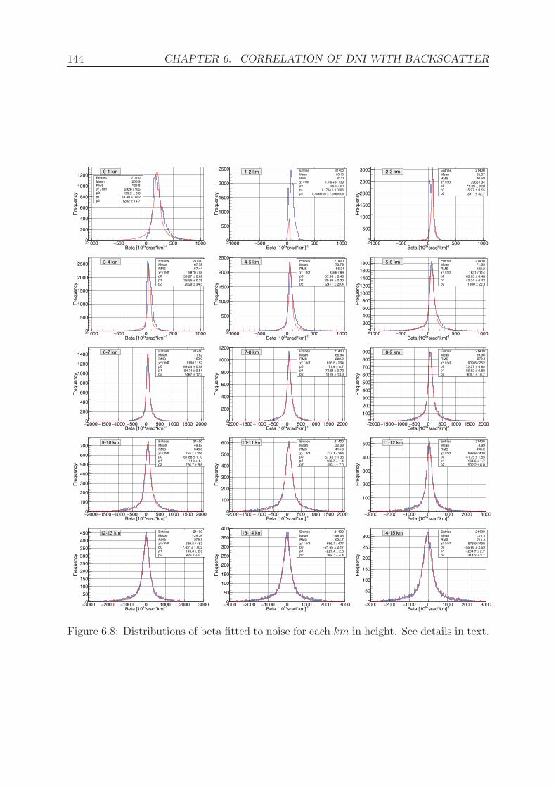
144 CHAPTER 6. CORRELATION OF DNI WITH BACKSCATTER
Entries 21400Mean 236.9RMS 126.5
/ ndf 2χ 2426 / 165p0 0.8± 199.9 p1 0.62± 63.48 p2 14.7± 1282
-1*srad*km]5Beta [101000− 500− 0 500 1000
Fre
quen
cy
0
200
400
600
800
1000
1200Entries 21400Mean 236.9RMS 126.5
/ ndf 2χ 2426 / 165p0 0.8± 199.9 p1 0.62± 63.48 p2 14.7± 1282
0-1 km Entries 21400Mean 85.13RMS 50.21
/ ndf 2χ 1.78e+04 / 39p0 0.1± 23.5 p1 0.0386± 0.1734 p2 7.556e+05± 1.749e+06
-1*srad*km]5Beta [101000− 500− 0 500 1000
Fre
quen
cy
0
500
1000
1500
2000
2500 Entries 21400Mean 85.13RMS 50.21
/ ndf 2χ 1.78e+04 / 39p0 0.1± 23.5 p1 0.0386± 0.1734 p2 7.556e+05± 1.749e+06
1-2 km Entries 21400Mean 65.07RMS 40.59
/ ndf 2χ 7965 / 34p0 0.31± 71.93 p1 0.15± 15.97 p2 42.7± 3371
-1*srad*km]5Beta [101000− 500− 0 500 1000
Fre
quen
cy
0
500
1000
1500
2000
2500
3000 Entries 21400Mean 65.07RMS 40.59
/ ndf 2χ 7965 / 34p0 0.31± 71.93 p1 0.15± 15.97 p2 42.7± 3371
2-3 km
Entries 21400Mean 67.78RMS 57.44
/ ndf 2χ 5870 / 58p0 0.69± 58.27 p1 0.25± 23.55 p2 34.3± 2629
-1*srad*km]5Beta [101000− 500− 0 500 1000
Fre
quen
cy
0
500
1000
1500
2000
2500Entries 21400Mean 67.78RMS 57.44
/ ndf 2χ 5870 / 58p0 0.69± 58.27 p1 0.25± 23.55 p2 34.3± 2629
3-4 km Entries 21400Mean 73.78RMS 85.21
/ ndf 2χ 3166 / 89p0 0.43± 57.43 p1 0.30± 29.86 p2 29.4± 2417
-1*srad*km]5Beta [101000− 500− 0 500 1000
Fre
quen
cy
0
500
1000
1500
2000
2500Entries 21400Mean 73.78RMS 85.21
/ ndf 2χ 3166 / 89p0 0.43± 57.43 p1 0.30± 29.86 p2 29.4± 2417
4-5 km Entries 21400Mean 71.55RMS 122.2
/ ndf 2χ 1631 / 114p0 0.48± 65.03 p1 0.42± 42.24 p2 22.1± 1860
-1*srad*km]5Beta [101000− 500− 0 500 1000
Fre
quen
cy
0
200
400
600
800
1000
1200
1400
1600
1800Entries 21400Mean 71.55RMS 122.2
/ ndf 2χ 1631 / 114p0 0.48± 65.03 p1 0.42± 42.24 p2 22.1± 1860
5-6 km
Entries 21400Mean 71.62RMS 163.9
/ ndf 2χ 1193 / 152p0 0.58± 69.04 p1 0.54± 54.71 p2 17.3± 1467
-1*srad*km]5Beta [102000− 1500− 1000− 500− 0 500 1000 1500 2000
Fre
quen
cy
0
200
400
600
800
1000
1200
1400Entries 21400Mean 71.62RMS 163.9
/ ndf 2χ 1193 / 152p0 0.58± 69.04 p1 0.54± 54.71 p2 17.3± 1467
6-7 km Entries 21400Mean 66.94RMS 222.2
/ ndf 2χ 816.8 / 204p0 0.7± 71.4 p1 0.72± 72.61 p2 13.3± 1126
-1*srad*km]5Beta [102000− 1500− 1000− 500− 0 500 1000 1500 2000
Fre
quen
cy
0
200
400
600
800
1000
1200Entries 21400Mean 66.94RMS 222.2
/ ndf 2χ 816.8 / 204p0 0.7± 71.4 p1 0.72± 72.61 p2 13.3± 1126
7-8 km Entries 21400Mean 59.98RMS 278.1
/ ndf 2χ 909.8 / 252p0 0.89± 72.27 p1 0.88± 89.52 p2 10.7± 909.1
-1*srad*km]5Beta [102000− 1500− 1000− 500− 0 500 1000 1500 2000
Fre
quen
cy
0
100
200
300
400
500
600
700
800
900 Entries 21400Mean 59.98RMS 278.1
/ ndf 2χ 909.8 / 252p0 0.89± 72.27 p1 0.88± 89.52 p2 10.7± 909.1
8-9 km
Entries 21400Mean 49.82RMS 346.8
/ ndf 2χ 755.1 / 306p0 1.10± 67.88 p1 1.1± 113 p2 8.6± 726.7
-1*srad*km]5Beta [102000− 1500− 1000− 500− 0 500 1000 1500 2000
Fre
quen
cy
0
100
200
300
400
500
600
700Entries 21400Mean 49.82RMS 346.8
/ ndf 2χ 755.1 / 306p0 1.10± 67.88 p1 1.1± 113 p2 8.6± 726.7
9-10 km Entries 21400Mean 32.08RMS 414.9
/ ndf 2χ 737.1 / 364p0 1.35± 57.45 p1 1.4± 138.7 p2 7.0± 593.1
-1*srad*km]5Beta [102000− 1500− 1000− 500− 0 500 1000 1500 2000
Fre
quen
cy
0
100
200
300
400
500
600 Entries 21400Mean 32.08RMS 414.9
/ ndf 2χ 737.1 / 364p0 1.35± 57.45 p1 1.4± 138.7 p2 7.0± 593.1
10-11 km Entries 21400Mean 3.99RMS 496.2
/ ndf 2χ 698.8 / 400p0 1.55± 41.75 p1 1.7± 164.6 p2 6.0± 502.2
-1*srad*km]5Beta [103000− 2000− 1000− 0 1000 2000 3000
Fre
quen
cy
0
100
200
300
400
500Entries 21400Mean 3.99RMS 496.2
/ ndf 2χ 698.8 / 400p0 1.55± 41.75 p1 1.7± 164.6 p2 6.0± 502.2
11-12 km
Entries 21400Mean 25.26−RMS 579.9
/ ndf 2χ 689.5 / 453p0 1.872± 7.431 p1 2.0± 193.8 p2 5.1± 426.7
-1*srad*km]5Beta [103000− 2000− 1000− 0 1000 2000 3000
Fre
quen
cy
0
50
100
150
200
250
300
350
400
450 Entries 21400Mean 25.26−RMS 579.9
/ ndf 2χ 689.5 / 453p0 1.872± 7.431 p1 2.0± 193.8 p2 5.1± 426.7
12-13 km Entries 21400Mean 46.45−RMS 652.7
/ ndf 2χ 666.7 / 477p0 2.17±21.65−p1 2.3±227.4−p2 4.4± 364.1
-1*srad*km]5Beta [103000− 2000− 1000− 0 1000 2000 3000
Fre
quen
cy
0
50
100
150
200
250
300
350
400Entries 21400Mean 46.45−RMS 652.7
/ ndf 2χ 666.7 / 477p0 2.17±21.65−p1 2.3±227.4−p2 4.4± 364.1
13-14 km Entries 21400Mean 71.1−RMS 711.1
/ ndf 2χ 573.9 / 490p0 2.53±55.86−p1 2.7±264.7−p2 3.7± 314.2
-1*srad*km]5Beta [103000− 2000− 1000− 0 1000 2000 3000
Fre
quen
cy
0
50
100
150
200
250
300Entries 21400Mean 71.1−RMS 711.1
/ ndf 2χ 573.9 / 490p0 2.53±55.86−p1 2.7±264.7−p2 3.7± 314.2
14-15 km
Figure 6.8: Distributions of beta fitted to noise for each km in height. See details in text.

6.2. MODELLING DIRECT NORMAL IRRADIANCE WITH LIDAR 145
Height [km]2 4 6 8 10 12 14
/ndf
2 χ
0
50
100
150
200
250
300
350
400
450
Figure 6.9: Goodness of the fit of the beta distribution to a noise distribution for each
km in height. See details in text.
the needed information in the atmosphere and taking the most valid signal from the
ceilometer and excluding the noise.
For this reason, the present study will be confined to the first 5 km, since the main
intent of this work is to show how the atmospheric variations affect the solar radiation.
6.2 Modelling Direct Normal Irradiance with lidar
Very often, the direct normal irradiance is not measured directly due to practical reasons,
and is derived instead from measurements of other readily available parameters such as
global irradiance or by using models such as radiative transfer models or satellite-based
models. However, the resulting modelled DNI data exhibits high discrepancies when com-
pared to ground measurements [155, 156]. A large part of these uncertainties is attributed
to inaccurate aerosol data used as input in the model. Aerosols play an important role
in the attenuation of DNI [5]. Aerosol optical depth (AOD) is one of the most impor-
tant parameters used to represent solar light extinction [6]. AOD can either be derived
from satellite observations, for instance with the MODerate resolution Imaging Spec-
troradiometer (MODIS) of NASA [10] or the Multi-angle Imaging SpectroRadiometer
(MISR) [9], or measured by ground-based sunphotometers, as done by NASA’s Aerosol
Robotic Network AERONET [8]. Chemical transport models such as MATCH (Model of
Atmospheric Transport and Chemistry) [157] and numerical weather prediction models
as used within the MACC (Monitoring Atmospheric Composition and Climate) project
[11] are also used to estimate AOD. Lidar-ceilometer measurements provide information

146 CHAPTER 6. CORRELATION OF DNI WITH BACKSCATTER
about the evolution and intensity of aerosols in the atmosphere, obtained from the mea-
surements of vertical backscatter profiles of the atmosphere. One of the main goals of
this thesis work is the study of the potential use of aerosol information, extracted from
the measurements of a lidar-ceilometer, for the assessment or the modelling of the direct
normal irradiance.
In the following sections the data of the CL51 ceilometer is used for the estimation
of DNI by establishing a relation between the daily variations of DNI and backscatter
atmospheric extinction around solar noon, under cloud-free conditions. The experiment
was carried out for a period of 12 months, from December 2012 to November 2013.
Atmospheric backscatter profiles as measured by the ceilometer were acquired at the
same time and location as the DNI measurements by a pyrheliometer, as described in
Chapter 4. The methodology to obtain the correlation between both measurements is
described below and consists of correlating the hourly DNI clearness index, Kn, to the
hourly backscatter measurements integrated over a column of 5 km in height. The results
of this technique were then compared to satellite-based model techniques and show the
potential use of aerosol information as measured by lidar-ceilometer for solar radiation
modelling.
6.2.1 Methodology
For the comparison of lidar backscatter measurements and DNI, only clear days in the
time interval 10 am to 1 pm, Doha local time, were selected. Clear days were chosen
because the purpose of this thesis is to study the effects of aerosols (and not clouds),
as measured by a lidar-ceilometer, on solar radiation. Moreover, eliminating cloudy
days avoids any inconsistencies arising from the possible presence of clouds above one
instrument and not the other. By clear day it is meant that, during the period between
10 am and 1 pm, the sky around the sun’s disk and along the lidar-ceilometer’s line of
view was free of visible clouds. The method used for selecting clear days was based on
the CL51 algorithm, visualised through Vaisala’s CL-VIEW software [158], which reports
cloud height information when detected. In addition, each individual DNI profile was
visually scrutinised and a comparison between both results (cloud reports and DNI) was
made to improve the correctness of the selection. Following this method and including
only days where both measurements were available, 214 clear days were selected, during
the period from Dec/2012 to Nov/2013. The Beta-model presented in this study is derived
using this sample of selected clear days.
The purpose of this study is to show how the dynamicity of the atmosphere as mea-
sured by a lidar-ceilometer is reflected in the variability of DNI. To detect these changes

6.2. MODELLING DIRECT NORMAL IRRADIANCE WITH LIDAR 147
in the atmosphere, the method adopted here consists of comparing, at a specific time of
the day, the day-to-day variation of the hourly averages of a normalised form of DNI,
the Kn index, which is the ratio of DNI to the extraterrestrial DNI at the top of the
atmosphere, with the day-to-day variation of the hourly-averaged backscatter lidar signal
integrated over the vertical column up to 5 km in height. This integrated backscatter
signal is hereby called for simplicity the Betatot coefficient; the limit of the maximum
height up to 5 km is discussed in Section 6.1. The extraterrestrial DNI for day n of the
year, in W/m2, was calculated following Equation 1.1.
The comparison was made in the hour that includes solar noon, from 11 am to 12
pm Doha local time (UTC+3 hours), so that the zenith angle of the sun is as close as
possible to the vertical direction of the lidar beam, thus having as similar amounts of
air mass as possible. Solar noon occurs for this location in Doha around 11:30 am, more
precisely between 11:16 and 11:48 am, depending on the time of the year; the solar zenith
angle at solar noon varies from about 2◦ in summer to about 48◦ in winter because of the
seasonal changes in solar declination angle. The use of Kn in the model, instead of DNI,
provides a sort of normalisation by taking into account the seasonal variations of DNI due
to changes in the sun-earth distance, allowing for better comparison of different times of
the year. To better understand the impact of different air masses throughout a year, all
possible sun zenith angles in a year period, at around solar noon, are depicted in Figure
6.10 for the site of the experiment. This angle varies slowly from day to day. However,
the variation is large through the year, which means that the amount of air mass seen by
the ceilometer is not always the same as that seen by the pyrheliometer, specially in the
winter season where the sun elevation is lower and thus sunlight traverses a longer path.
In this section, this additional distance is assumed to have a negligible effect. Indeed, and
as seen in Section 6.1, the variability of atmospheric contents is mostly confined to lower
heights, and therefore all the relevant information, which is contained in these heights, is
considered as included in the 5 km integration of the vertical column considered here.
6.2.2 Lidar-ceilometer measurements
As stated before, backscatter intensities were measured by a CL51 ceilometer, pointing
vertically upwards and operating continuously for the acquisition of backscatter profiles
and detection of aerosol structures in the atmosphere. As also discussed, aerosol infor-
mation is represented by a backscatter coefficient reported each 36 s up to 15 km, in
10-m steps. Betatot, the integrated hourly average of the backscatter coefficient up to
5 km, was obtained by calculating first the hourly-averaged backscatter coefficients for
each height step, from the 36-s backscatter coefficients acquired by the lidar, and then the

148 CHAPTER 6. CORRELATION OF DNI WITH BACKSCATTER
Day0 50 100 150 200 250 300 350 400
Deg
rees
0
10
20
30
40
50
Figure 6.10: Daily variation of the zenith angle of the sun around solar noon, from 1
January to 31 December for Doha, Qatar.
averaged coefficients were summed from ground level up to 5 km. The plot of the daily
variation of this sum at the noon hour, i.e., from 11 am to 12 pm, is displayed in Figure
6.11 for the 214 selected clear days. The variations in Betatot show the dynamicity of
the atmosphere in Doha. It is observed that Betatot has higher values in the summer
season. This is mainly due to the atmospheric conditions in Doha during summer (more
precisely, from April to September), when the atmosphere is more highly loaded with
aerosols and dust events are more prone to occur. The highest values of Betatot observed
in the figure are related to dust storm events, as will be discussed in Section 6.2.3.
Day of the year
335
365 30 60 90 120
150
180
210
240
270
300
330
-1*s
rad*
km]
5B
eta
[10
0
20
40
60
80
100
120310×
Figure 6.11: Daily variation of integrated backscatter around solar noon for cloud-free
days in a one-year period. Non-clear days are shown with Betatot=0.

6.2. MODELLING DIRECT NORMAL IRRADIANCE WITH LIDAR 149
6.2.3 DNI measurements
For the calculation of hourly averages of DNI, only one-minute DNI data which pass
the quality control tests were considered. Gap-filling was not needed, because in all the
selected clear days, there were no values missing or failing the quality tests, so all hourly
averages used here were obtained from 60 one-minute values. In Figure 6.12, DNI hourly
averages for all the selected clear days around solar noon are shown. DNI exhibits large
day-to-day fluctuations with no obvious seasonal changes during the year, depending
mainly on the atmospheric extinction of solar radiation. Therefore, within one month
one can find days with high DNI hourly average at noon while the next day shows a
much lower value. The hourly DNI averages fall mostly within a band from 600 to 900
W/m2, except in periods where dust storms occur and significantly reduce the amount
of DNI. A qualitative inverse relation can be seen between the Betatot and DNI graphs.
For instance, the lowest DNI (under 200 W/m2) values in Figure 6.12 correspond to the
highest Betatot values in Figure 6.11. The correlation is more clearly shown and discussed
in the next section. During summer, lower values of DNI are found due to higher aerosol
levels. The maximum hourly average of DNI around solar noon was 969.1 W/m2, found
on 22 March, and the minimum was 75.5 W/m2, found on 6 April. As mentioned in
Section 6.2.1, DNI was not used directly for the development of the model, but through
the normalised DNI clearness index Kn.
Day of the year
335
365 30 60 90 120
150
180
210
240
270
300
330
]2D
NI [
W/m
0
200
400
600
800
1000
Figure 6.12: Daily variation of hourly averages of DNI around solar noon for cloud-free
days in a one-year period. Non-clear days are shown with DNI=0.

150 CHAPTER 6. CORRELATION OF DNI WITH BACKSCATTER
6.2.4 Correlation of DNI and ceilometer signal
In general and all through the year, the atmosphere in Qatar is highly loaded with
aerosols, mainly due to desert dust, high humidity and the occurrence of dust storms,
but also because of industrial emissions. The direct and indirect effects of aerosols on the
extinction of solar radiation are widely studied in the literature [159, 160, 161]. In this
thesis work, the correlation between aerosols as extracted from lidar-ceilometer backscat-
ter measurements and DNI measurements is shown in an attempt to quantify this effect,
resulting in a model for the derivation of DNI from ceilometer measurements only. For
the rest of this chapter, this model is referred to as the Beta-model.
Figure 6.13 shows the relation between hourly Kn and the Betatot coefficient in Doha
following the method described in Section 6.2.1. It is observed from the experimental
data that Kn seems to decrease exponentially with Betatot and an exponential function is
found to fit well both measurements, a behaviour similar to the Lambert-Beer exponential
law [100], which describes the decrease of radiation traversing a medium. The fitted
equation can be written as follows:
Kn = exp(slope ·Betatot+ const), (6.2)
where Betatot is the sum of the hourly-averaged backscatter lidar signals at noon, up to
a height of 5 km; slope and const are parameters obtained from the fit and are shown on
the statistics box of Figure 6.13.
-1*srad*km]5Betatot [1020 40 60 80 100 120
310×
Kn
0
0.1
0.2
0.3
0.4
0.5
0.6
0.7Constant 0.02442± -0.1772
Slope 4.71e-007± -8.941e-006
Constant 0.02442± -0.1772
Slope 4.71e-007± -8.941e-006
Figure 6.13: Correlation between Kn and integrated backscatter at solar noon in Doha.
The presented exponential function fits well the Kn measurements as a function of
Betatot. The relative bias and RMSE, as defined in Section 6.2.5 and calculated between
the fit function and the ground measurements are (all values in %) 0.0695 and 11.164 for

6.2. MODELLING DIRECT NORMAL IRRADIANCE WITH LIDAR 151
Kn, and 0.156 and 11.101 for DNI, respectively. Despite the limited integration height of
5 km, a close correlation is found between both measurements and this is emphasised in
the next paragraphs, where the proposed Beta-model is shown to provide good statistical
measures when validated against ground-measured DNI.
6.2.5 Model validation
In order to validate the Beta-model, results from different data sets and different periods
of time are discussed in the following.
Three validations were made using ground measurements acquired by the same solar
radiation monitoring station, at QEERI’s solar resource assessment site; two of them
were performed using the same sample of the selected clear days from December 2012 to
November 2013, but at different hours, and the third validation was made with a new
sample of clear days selected for the next twelve months, i.e., from December 2013 to
November 2014:
• The first validation was done from December 2012 to November 2013, with the hour
preceding the one used to derive the Beta-model, that is, Kn at 11 am (from 10 to
11 am).
• The second validation was done from December 2012 to November 2013, with the
hour after, that is, Kn at 1 pm (from 12 to 1 pm).
• The third validation was made for a different period (the following year), from
December 2013 to November 2014, for the same hour used to derive the Beta-model,
at 12 pm (from 11 am to 12 pm).
Validating the Beta-model using 2 different hours in the day tests the validity of the
model at a slightly wider interval of solar zenith angles or, equivalently, air masses. The
clear days for the second year were selected following the same methodology described in
Section 6.2.1.
As seen in Section 1.5, solar radiation at ground level can also be derived from satellite
observations, with data currently available for all sky conditions, from several commercial
providers such as GeoModel Solar and SoDa services, or for free such as from the NASA-
SSE database; models and databases also exist for clear sky conditions [162, 144]. In
order to have an independent reference for comparison, three sets of additional analyses
were done; the first set uses the SolarGIS database to derive hourly Kn at 11 am and 1
pm, from December 2012 to November 2013. The second and third ones use McClear-
derived hourly Kn data, at 11 am and 1 pm from December 2012 to November 2013, and
12 pm for the data from December 2013 to November 2014.

152 CHAPTER 6. CORRELATION OF DNI WITH BACKSCATTER
All these tests are summarised in Table 6.1.
Period: Dec/2012 – Nov/2013 Dec/2013 – Nov/2014
Hour: 11 12 13 11 12 13
Beta-model vs. ground � � � � � �
SolarGIS model vs. ground � � � � � �
McClear model vs. ground � � � � � �
Table 6.1: Validations of the different models with ground measurements.
Validations at 11 am and 1 pm, December 2012 to November 2013
For these validations, Kn and DNI were derived from the Beta-model for all the selected
clear days by using Equation 6.2 and the Betatot values obtained for hour 11 am and
hour 1 pm. Figure 6.14 shows the scatter plot comparison between the Beta-model-
estimated hourly DNI (bottom) and Kn (top) and the corresponding averages of DNI
and Kn calculated from DNI measurements at 11 am (left plots) and at 1 pm (right
plots).
To provide a basis for comparing the statistical results of the previous validation,
the hourly values of Kn were calculated using satellite data and validated against the
same ground measurements. Figures 6.15 and 6.16 show the comparison with ground
measurements of calculated hourly Kn and DNI from the SolarGIS satellite service and
the McClear database, respectively, for 11 am and 1 pm.
Validation at 12 pm, from December 2013 to November 2014
The third validation of the Beta-model was made at 12 pm, with data of the next twelve
months. Using a different year allows to test the validity of the model under different
atmospheric cloudless conditions from those used for the derivation of the model. The
results are compared with the validation of the McClear-derived hourly Kn with ground
measurements. The left-hand side graph in Figure 6.17 shows the scatter plot comparison
between the Beta-model-estimated hourly Kn and the corresponding averages of Kn cal-
culated from DNI measurements. The right-hand side graph shows a similar comparison,
for McClear-derived hourly Kn.
It is noted that the scatter plots of modelled against measured DNI, on the bottom
rows of Figures 6.14 to 6.17, are almost identical to the Kn scatter plots on the top row
of the same figures.

6.2. MODELLING DIRECT NORMAL IRRADIANCE WITH LIDAR 153
Kn meas.0 0.1 0.2 0.3 0.4 0.5 0.6 0.7 0.8 0.9 1
Kn
Bet
aMod
el
0
0.1
0.2
0.3
0.4
0.5
0.6
0.7
0.8
0.9
1
Hour = 11
Kn meas.0 0.1 0.2 0.3 0.4 0.5 0.6 0.7 0.8 0.9 1
Kn
Bet
aMod
el
0
0.1
0.2
0.3
0.4
0.5
0.6
0.7
0.8
0.9
1
Hour = 13
DNI meas.0 200 400 600 800 1000
DN
I Bet
aMod
el
0
200
400
600
800
1000
Hour = 11
DNI meas.0 200 400 600 800 1000
DN
I Bet
aMod
el
0
200
400
600
800
1000
Hour = 13
Figure 6.14: Comparison of the hourly values of Kn (top) and DNI (bottom) obtained
through the Beta-model vs. the values calculated from DNI measurements, at the hour
from 10 to 11 am (left), and from 12 to 1 pm (right). The one-to-one line is shown in
red. See Tables 6.2 and 6.3 for the statistical results.
Results
In clear-sky conditions, aerosols are the main factor affecting the extinction of DNI. Errors
in the estimation of aerosol data used as input in solar radiation models, may result in
DNI uncertainties in the range of 15% to 20%, specifically in regions like the Arabian
Peninsula, where dust storms strike occasionally and contribute to changes in the aerosol
regime [5].
In the SolarGIS calculation scheme, aerosols are represented by the AOD derived from
a chemical-transport model, the MACC database lead by ECMWF (European Centre for
Medium Range Weather Forecast) [11], which characterises the overall radiative effect of
aerosols in terms of daily AOD values (summarised from 6-hourly) at 550 nm, with a
spatial resolution of 125 km. It was demonstrated in [163] that using daily AOD data
from the MACC database, instead of monthly, significantly improves the calculation of
DNI. The SolarGIS model has demonstrated good results when compared to ground
measurements in atmospheric conditions similar to the ones encountered in Qatar [164].
McClear is a fully physical clear-sky model to estimate solar radiation at ground level
under clear sky conditions. Its inputs of aerosols, ozone column and water vapour come

154 CHAPTER 6. CORRELATION OF DNI WITH BACKSCATTER
Kn meas.0 0.1 0.2 0.3 0.4 0.5 0.6 0.7 0.8 0.9 1
Kn
SG
0
0.1
0.2
0.3
0.4
0.5
0.6
0.7
0.8
0.9
1
Hour = 11
Kn meas.0 0.1 0.2 0.3 0.4 0.5 0.6 0.7 0.8 0.9 1
Kn
SG
0
0.1
0.2
0.3
0.4
0.5
0.6
0.7
0.8
0.9
1
Hour = 13
DNI meas.0 200 400 600 800 1000
DN
I SG
0
200
400
600
800
1000
Hour = 11
DNI meas.0 200 400 600 800 1000
DN
I SG
0
200
400
600
800
1000
Hour = 13
Figure 6.15: Comparison of the hourly values of Kn (top) and DNI (bottom) obtained
from SolarGIS vs. the values calculated from DNI measurements, (left) at the hour from
10 to 11 am and (right) at the hour from 12 to 1 pm. The one-to-one line is shown in
red. See Tables 6.2 and 6.3 for the statistical results.
primarily from the MACC project. It is mainly based on the use of the abaci approach
(tables for computation) and interpolation functions, which enable the model to reproduce
data as estimated by the radiation transfer model libRadtran, but in a much faster way
for use in real-time routine applications. Aerosol information as used by the McClear
model consists of aerosol optical depth at 550 nm, Angstrom coefficient, and aerosol
type: urban, continental clean, continental polluted, continental average, maritime clean,
maritime polluted, maritime tropical, antarctic, and desert. The McClear model has been
validated at several BSRN stations giving good results [162].
To obtain a quantitative comparison between the performance of these models and
the Beta-model, the following statistical indicators were calculated:
• The mean bias error (MBE), which is the difference between the mean value of the
modelled values (Kn or DNI) and the mean value of the corresponding measure-
ments, is given in radiation units by the formula:
MBE =1
Np
Np∑i=1
(Mi −Gi) (6.3)

6.2. MODELLING DIRECT NORMAL IRRADIANCE WITH LIDAR 155
Kn meas.0 0.1 0.2 0.3 0.4 0.5 0.6 0.7 0.8 0.9 1
Kn
McC
lear
0
0.1
0.2
0.3
0.4
0.5
0.6
0.7
0.8
0.9
1
Hour = 11
Kn meas.0 0.1 0.2 0.3 0.4 0.5 0.6 0.7 0.8 0.9 1
Kn
McC
lear
0
0.1
0.2
0.3
0.4
0.5
0.6
0.7
0.8
0.9
1
Hour = 13
DNI meas.0 200 400 600 800 1000
DN
I McC
lear
0
200
400
600
800
1000
Hour = 11
DNI meas.0 200 400 600 800 1000
DN
I McC
lear
0
200
400
600
800
1000
Hour = 13
Figure 6.16: Comparison of the hourly values of Kn (top) and DNI (bottom) obtained
from McClear vs. the values calculated from DNI measurements, (left) at the hour from
10 to 11 am and (right) at the hour from 12 to 1 pm. The one-to-one line is shown in
red. See Tables 6.2 and 6.3 for the statistical results.
where Np is the total number of data pairs (in this case, one for each selected day),
Mi are the modelled values and Gi are the reference (ground-measured) values.
MBE allows to identify systematic errors.
• The root-mean-square error (RMSE) is also given in radiation units and compares
time-coincident modelled and measured data pairs, and is calculated as
RMSE =
√∑Npi=1(Mi −Gi)2
Np(6.4)
where Np is the total number of data pairs (in this case, 214, one for each selected
day), Mi are the modelled values and Gi are the reference (measured) values.
• The relative MBE (rMBE) and relative RMSE (rRMSE), which are the MBE and
RMSE divided by the mean value of the measured quantity (Kn or DNI) and usually
presented as percentage.
• The correlation factor measures the strength and direction of a linear relationship
between the modelled and corresponding measured data points. If the relationship

156 CHAPTER 6. CORRELATION OF DNI WITH BACKSCATTER
Kn meas.0 0.1 0.2 0.3 0.4 0.5 0.6 0.7 0.8 0.9 1
Kn
Bet
aMod
el
0
0.1
0.2
0.3
0.4
0.5
0.6
0.7
0.8
0.9
1
Hour = 12
Kn meas.0 0.1 0.2 0.3 0.4 0.5 0.6 0.7 0.8 0.9 1
Kn
McC
lear
0
0.1
0.2
0.3
0.4
0.5
0.6
0.7
0.8
0.9
1
Hour = 12
DNI meas.0 200 400 600 800 1000
DN
I Bet
aMod
el
0
200
400
600
800
1000
Hour = 12
DNI meas.0 200 400 600 800 1000
DN
I McC
lear
0
200
400
600
800
1000
Hour = 12
Figure 6.17: (Left) Comparison at the hour from 11 am to 12 pm of the hourly values ofKn
(top) and DNI (bottom) obtained through the Beta-model vs. the values calculated from
DNI measurements, from December 2013 to November 2014. (Right) Same comparison,
but for McClear-derived data. The one-to-one line is shown in red. See Table 6.4 for the
statistical results.
is strong and positive (negative), this factor is close to 1 (-1). A weak or non-exitent
correlation results in a factor close to 0. The formula is:
Correl. =Np
∑(MiGi)− (
∑Mi)(
∑Gi)√
Np(∑
M2i )− (
∑Mi)2
√Np(
∑G2
i )− (∑
Gi)2(6.5)
Tables 6.2 and 6.3 present the overall statistical comparison results of both Kn and
DNI at 11 am and 1 pm, respectively, for the same selected clear days that were used
to derive the model (from December 2012 to November 2013), whereas Table 6.4 shows
the same, but at 12 pm, for the data set of the next twelve months (December 2013 to
November 2014). Hourly Kn and DNI are derived from each of the three models (Beta-
model, SolarGIS and McClear) and compared against the corresponding ground-measured
values. From these tables, it is evident that the Beta-model’s statistical results are indeed
good, comparable to the results of the McClear-derived values and even improving the
MBE, RMSE and correlation factor with respect to the results from the SolarGIS-derived
values. The validation of the Beta-model using an independent set of data derived from
values collected the following year, also shows good results comparable to those of the

6.2. MODELLING DIRECT NORMAL IRRADIANCE WITH LIDAR 157
McClear model, a result which demonstrates the validity of the Beta-model in different
aerosol load conditions. It must be noted, as well, that for the validation made at one
hour before and one hour after the hour for which the model was derived, even though the
solar zenith angles during both hours mostly overlap through the year, a difference still
remains, yet the model provides good results, supporting the use of Kn as a normalised
parameter for the model and giving evidence that the Beta-model works for a relatively
wide range of solar zenith angles.
Model Np MBE rMBE RMSE rRMSE Correl.
Kn
Beta-model 214 0.010 1.861 0.056 10.826 0.819
SolarGIS model 214 -0.024 -4.663 0.071 13.794 0.732
McClear model 214 -0.015 -2.951 0.058 11.277 0.831
DNI
Beta-model 214 13.957 1.979 76.673 10.869 0.832
SolarGIS model 214 -32.882 -4.661 96.708 13.710 0.754
McClear model 214 -20.327 -2.882 78.301 11.100 0.849
Table 6.2: Statistical indicators of the comparison of modelled against measured Kn
(dimensionless) and DNI (W/m2), at the hour from 10 to 11 am, from Dec/2012 to
Nov/2013. rMBE and rRMSE are in %.
Model Np MBE rMBE RMSE rRMSE Correl.
Kn
Beta-model 213 -0.001 -0.285 0.061 11.916 0.796
SolarGIS model 213 -0.027 -5.351 0.081 15.850 0.672
McClear model 213 -0.004 -0.813 0.060 11.738 0.813
DNI
Beta-model 213 -1.024 -0.147 82.568 11.873 0.817
SolarGIS model 213 -37.424 -5.382 109.99 15.817 0.698
McClear model 213 -5.404 -0.777 80.609 11.592 0.832
Table 6.3: Statistical indicators of the comparison of modelled against measured Kn (di-
mensionless) and DNI (W/m2), at the hour from 12 to 1 pm, from Dec/2012 to Nov/2013.
rMBE and rRMSE are in %.
Although the comparisons between the hourly satellite data as derived from SolarGIS
and hourly ground measurements (seen in Tables 6.2 and 6.3) show fairly good statistical

158 CHAPTER 6. CORRELATION OF DNI WITH BACKSCATTER
Model Np MBE rMBE RMSE rRMSE Correl.
Kn
Beta-model 213 -0.017 -3.083 0.063 11.443 0.689
McClear model 213 -0.032 -5.768 0.060 11.007 0.849
DNI
Beta-model 213 -21.562 -2.900 84.765 11.400 0.737
McClear model 213 -42.112 -5.663 81.198 10.920 0.869
Table 6.4: Statistical indicators of the comparison of modelled against measured Kn
(dimensionless) and DNI (W/m2), at the hour from 11 am to 12 pm, for the data set of
the period December 2013 to November 2014. rMBE and rRMSE are in %.
results, the observed errors may be attributed to the low spatial as well as temporal
resolution of the aerosol data; daily AOD data, as used in the SolarGIS model, may
not be sufficient to capture the high fluctuations and variability of aerosols in Doha,
specially in dust storm events. Improvement in the chemical transportation model for the
derivation of the aerosol data, considering the spectral sensitivity of AOD, and increasing
the spatial and temporal resolution may be needed to achieve better results for modelling
DNI using satellite observations in the Arabian Peninsula. In contrast, the McClear model
uses higher temporal resolution data of aerosols (3-hourly), hence the better comparison
results. The Beta-model, even though it is only based on one input, uses aerosol data
(backscatter) with an even higher temporal resolution of one hour, measured on-site,
reflecting the actual local conditions; these improved spatial and temporal resolutions
contribute to its good performance when compared with ground measurements.
6.2.6 BetaCos-model
Although the Beta-model shows good results when its validation is compared to satellite
validation, it is still presenting errors which could be mostly attributed to the different
viewing angles between the two devices, measuring the backscatter on the one hand and
DNI on the other hand. This observation is more noticeable during the winter season,
where the sun around solar noon exhibits low elevation angles in the sky, as seen in Figure
6.10. In an attempt to improve the statistical results of the Beta-model, another model,
called here BetaCos-model, was developed by using the same methodology described
in Section 6.2.1, but instead of using the Betatot coefficient for DNI derivation, it was
decided to use an hourly average of a modified Betatot coefficient, ‘BetaCos’, defined

6.2. MODELLING DIRECT NORMAL IRRADIANCE WITH LIDAR 159
here as the Betatot coefficient modified by the zenith angle as follows:
BetaCos =
Nmin∑min=1
betamin
cos θz
Nmin, (6.6)
where BetaCos is the modified hourly Betatot, betamin is the 1-minute-averaged beta
coefficient and θz is the zenith angle at that same minute; the sum runs over all the
minutes with data within the hour (a maximum of 60).
The idea behind the use of this modified Betatot, is to add an additional scattering
volume to the lidar beam’s path equivalent to the extra path traversed by the solar
radiation, which depends on the zenith angle and is more pronounced in the winter
season. The resulting BetaCos-model relating the hourly Kn and the BetaCos coefficient,
for the selected clear days at around solar noon, is shown in Figure 6.18. It is observed
that Kn seems also to decrease exponentially with BetaCos and an exponential function
is fitted to the data, similarly to Equation 6.2. The fitted equation is written as follows:
Kn = exp(slope ·BetaCos+ const), (6.7)
where slope and const are parameters obtained from the fit and are shown on the statistics
box of Figure 6.18.
-1*srad*km]5BetaCos [1020 40 60 80 100 120
310×
Kn
0.1
0.2
0.3
0.4
0.5
0.6
0.7
0.8
0.9
1Constant 0.02743± -0.04914
Slope 4.781e-007± -1.021e-005
Constant 0.02743± -0.04914
Slope 4.781e-007± -1.021e-005
Figure 6.18: Correlation between Kn and the modified Betatot coefficient, BetaCos, at
solar noon in Doha.
For comparison with the Beta-model, the relative bias and RMSE were calculated
between the fit function and the ground measurements and give (all values in %) 0.032
and 10.330 for Kn, and 0.0059 and 10.231 for DNI, respectively. These results are slightly
better than those of the Beta-model shown in Section 6.2.4.

160 CHAPTER 6. CORRELATION OF DNI WITH BACKSCATTER
BetaCos-model validation
As in the case of the Beta-model, the BetaCos-model was validated against ground mea-
surements. Kn and DNI are derived from the BetaCos-model and compared against the
corresponding ground-measured values, as shown in the DNI and Kn scatter plots in
Figures 6.19 and 6.20, for the hours 11 am and 1 pm of the same selected clear days that
were used to derive the model (from December 2012 to November 2013), and at 12 pm
for the data set of the next twelve months (December 2013 to November 2014).
Kn meas.0 0.1 0.2 0.3 0.4 0.5 0.6 0.7 0.8 0.9 1
Kn
Bet
aCos
Mod
el
0
0.1
0.2
0.3
0.4
0.5
0.6
0.7
0.8
0.9
1
Hour = 11
Kn meas.0 0.1 0.2 0.3 0.4 0.5 0.6 0.7 0.8 0.9 1
Kn
Bet
aCos
Mod
el
0
0.1
0.2
0.3
0.4
0.5
0.6
0.7
0.8
0.9
1
Hour = 13
DNI meas.0 200 400 600 800 1000
DN
I Bet
aCos
Mod
el
0
200
400
600
800
1000
Hour = 11
DNI meas.0 200 400 600 800 1000
DN
I Bet
aCos
Mod
el
0
200
400
600
800
1000
Hour = 13
Figure 6.19: Comparison at two hours: from from 10 am to 11 am (left) and from 12 pm
to 1 pm (right) of the hourly values of Kn (top) and DNI (bottom) obtained through the
BetaCos-model vs. the values calculated from DNI measurements, from December 2012
to November 2013. The one-to-one line is shown in red. See Tables 6.5 and 6.6 for the
statistical results.
Tables 6.5 and 6.6 include the overall statistical comparison results of both Kn and
DNI at 11 am and 1 pm from December 2012 to November 2013. Table 6.7 shows the
same, but at 12 pm, for the data set of the period from December 2013 to November 2014.
The statistical results of the Beta-model are also shown in these tables for comparison.
It is evident that the BetaCos-model’s results are indeed good, but no clear improvement
over the Beta-model is seen for the ranges of zenith angles tested here.
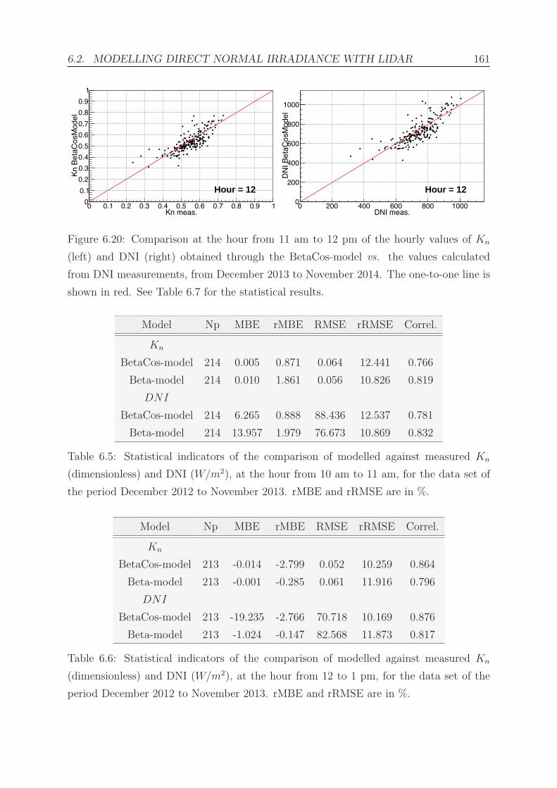
6.2. MODELLING DIRECT NORMAL IRRADIANCE WITH LIDAR 161
Kn meas.0 0.1 0.2 0.3 0.4 0.5 0.6 0.7 0.8 0.9 1
Kn
Bet
aCos
Mod
el
0
0.1
0.2
0.3
0.4
0.5
0.6
0.7
0.8
0.9
1
Hour = 12
DNI meas.0 200 400 600 800 1000
DN
I Bet
aCos
Mod
el
0
200
400
600
800
1000
Hour = 12
Figure 6.20: Comparison at the hour from 11 am to 12 pm of the hourly values of Kn
(left) and DNI (right) obtained through the BetaCos-model vs. the values calculated
from DNI measurements, from December 2013 to November 2014. The one-to-one line is
shown in red. See Table 6.7 for the statistical results.
Model Np MBE rMBE RMSE rRMSE Correl.
Kn
BetaCos-model 214 0.005 0.871 0.064 12.441 0.766
Beta-model 214 0.010 1.861 0.056 10.826 0.819
DNI
BetaCos-model 214 6.265 0.888 88.436 12.537 0.781
Beta-model 214 13.957 1.979 76.673 10.869 0.832
Table 6.5: Statistical indicators of the comparison of modelled against measured Kn
(dimensionless) and DNI (W/m2), at the hour from 10 am to 11 am, for the data set of
the period December 2012 to November 2013. rMBE and rRMSE are in %.
Model Np MBE rMBE RMSE rRMSE Correl.
Kn
BetaCos-model 213 -0.014 -2.799 0.052 10.259 0.864
Beta-model 213 -0.001 -0.285 0.061 11.916 0.796
DNI
BetaCos-model 213 -19.235 -2.766 70.718 10.169 0.876
Beta-model 213 -1.024 -0.147 82.568 11.873 0.817
Table 6.6: Statistical indicators of the comparison of modelled against measured Kn
(dimensionless) and DNI (W/m2), at the hour from 12 to 1 pm, for the data set of the
period December 2012 to November 2013. rMBE and rRMSE are in %.

162 CHAPTER 6. CORRELATION OF DNI WITH BACKSCATTER
Model Np MBE rMBE RMSE rRMSE Correl.
Kn
BetaCos-model 213 -0.012 -2.141 0.056 10.300 0.776
Beta-model 213 -0.017 -3.083 0.063 11.443 0.689
DNI
BetaCos-model 213 -15.250 -2.051 76.289 10.260 0.803
Beta-model 213 -21.562 -2.900 84.765 11.400 0.737
Table 6.7: Statistical indicators of the comparison of modelled against measured Kn
(dimensionless) and DNI (W/m2), at the hour from 11 am to 12 pm, for the data set of
the period December 2013 to November 2014. rMBE and rRMSE are in %.
6.2.7 BetaCos-model in a wider zenith angle range
It was shown that the performance of the BetaCos-model is comparable to the Beta-
model. The reason is that the BetaCos-model was developed based on data resulting
from the selection of clear days around solar noon. In order to expand the applicability
of this model, clear days for the period Dec/2012 to Nov/2013 were selected using the
methodology described in Section 6.2.1, but in a wider window of time, that is, from
7 am to 4 pm. The data based on this selection is used for the derivation of the new
BetaCos-model, following the same reasoning as in Section 6.2.6: a model relating the
hourly Kn and the BetaCos coefficient as shown in Figure 6.21. For all the hours from 7
am to 4 pm, Kn and BetaCos are fitted with an exponential function, written as follows:
Kn = exp(slope ·BetaCos+ const), (6.8)
where BetaCos is calculated from Equation 6.6 for all the hours between 7 am and 4 pm,
and slope and const are parameters obtained from the fit and are shown on the statistics
box of Figure 6.21.
Validation
The BetaCos-model presented in 6.2.7 was validated against ground measurements. Kn
and DNI are derived from the BetaCos-model and compared against the corresponding
ground-measured values, as shown in the DNI and Kn scatter plots in Figures 6.22 for
the hours from 7 am to 4 pm, using a newly selected set of clear days from the next
twelve-month period (December 2013 to November 2014). In order to have a reference
for the comparison, the same validation (using the same data set) is performed with data
derived from the McClear database and shown in the same figure.

6.2. MODELLING DIRECT NORMAL IRRADIANCE WITH LIDAR 163
-1*srad*km]5) [10zθBeta/cos(0 100 200 300 400 500 600
310×
nK
0
0.1
0.2
0.3
0.4
0.5
0.6
0.7 Constant 0.01049±0.08824−
Slope 07− 1.494e±06−9.097e−
Constant 0.01049±0.08824−
Slope 07− 1.494e±06−9.097e−
7-8 8-99-10 10-1111-12 12-1313-14 14-1515-16
Figure 6.21: Correlation between Kn and the modified Betatot coefficient BetaCos for
all the clear days from 7 am to 4 pm, for the period Dec/2012 to Nov/2013 in Doha.
Kn meas.0 0.1 0.2 0.3 0.4 0.5 0.6 0.7 0.8 0.9 1
Kn
Bet
aCos
Mod
el
0
0.1
0.2
0.3
0.4
0.5
0.6
0.7
0.8
0.9
1
DNI meas.0 200 400 600 800 1000
DN
I Bet
aCos
Mod
el
0
200
400
600
800
1000
Kn meas.0 0.1 0.2 0.3 0.4 0.5 0.6 0.7 0.8 0.9 1
Kn
McC
lear
0
0.1
0.2
0.3
0.4
0.5
0.6
0.7
0.8
0.9
1
DNI meas.0 200 400 600 800 1000
DN
I McC
lear
0
200
400
600
800
1000
Figure 6.22: Comparison of the hourly values of Kn (left) and DNI (right) obtained
through the BetaCos-model (top figures) and the McClear model (bottom figures) vs.
the values calculated from DNI measurements, from December 2013 to November 2014,
for hours 8 to 16 (from 7:01 to 16:00). The one-to-one line is shown in red. See Table 6.8
for the statistical results.
Table 6.8 presents the overall statistical comparison results of both Kn and DNI for
the BetaCos-model and the McClear model, for the hours from 7 am to 4 pm, for the
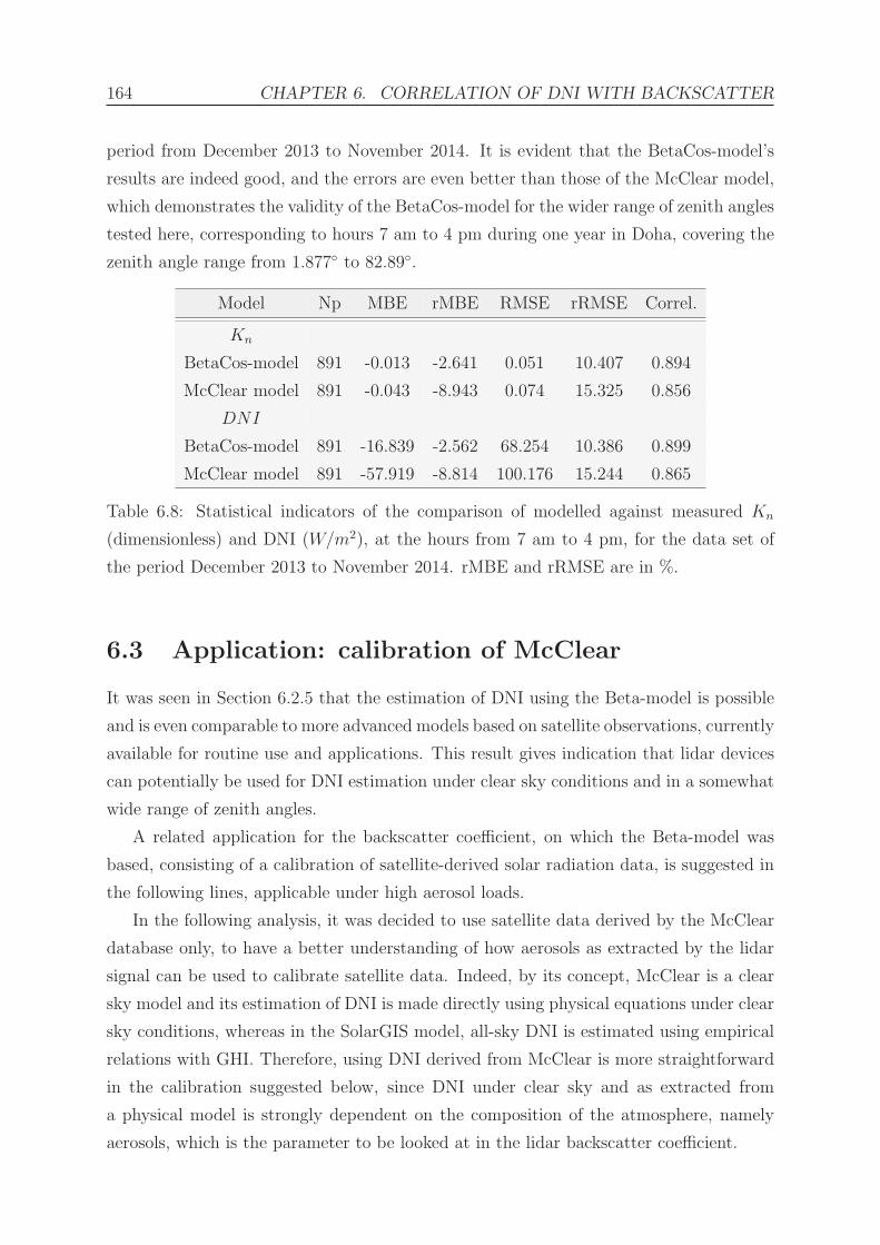
164 CHAPTER 6. CORRELATION OF DNI WITH BACKSCATTER
period from December 2013 to November 2014. It is evident that the BetaCos-model’s
results are indeed good, and the errors are even better than those of the McClear model,
which demonstrates the validity of the BetaCos-model for the wider range of zenith angles
tested here, corresponding to hours 7 am to 4 pm during one year in Doha, covering the
zenith angle range from 1.877◦ to 82.89◦.
Model Np MBE rMBE RMSE rRMSE Correl.
Kn
BetaCos-model 891 -0.013 -2.641 0.051 10.407 0.894
McClear model 891 -0.043 -8.943 0.074 15.325 0.856
DNI
BetaCos-model 891 -16.839 -2.562 68.254 10.386 0.899
McClear model 891 -57.919 -8.814 100.176 15.244 0.865
Table 6.8: Statistical indicators of the comparison of modelled against measured Kn
(dimensionless) and DNI (W/m2), at the hours from 7 am to 4 pm, for the data set of
the period December 2013 to November 2014. rMBE and rRMSE are in %.
6.3 Application: calibration of McClear
It was seen in Section 6.2.5 that the estimation of DNI using the Beta-model is possible
and is even comparable to more advanced models based on satellite observations, currently
available for routine use and applications. This result gives indication that lidar devices
can potentially be used for DNI estimation under clear sky conditions and in a somewhat
wide range of zenith angles.
A related application for the backscatter coefficient, on which the Beta-model was
based, consisting of a calibration of satellite-derived solar radiation data, is suggested in
the following lines, applicable under high aerosol loads.
In the following analysis, it was decided to use satellite data derived by the McClear
database only, to have a better understanding of how aerosols as extracted by the lidar
signal can be used to calibrate satellite data. Indeed, by its concept, McClear is a clear
sky model and its estimation of DNI is made directly using physical equations under clear
sky conditions, whereas in the SolarGIS model, all-sky DNI is estimated using empirical
relations with GHI. Therefore, using DNI derived from McClear is more straightforward
in the calibration suggested below, since DNI under clear sky and as extracted from
a physical model is strongly dependent on the composition of the atmosphere, namely
aerosols, which is the parameter to be looked at in the lidar backscatter coefficient.

6.3. APPLICATION: CALIBRATION OF MCCLEAR 165
By looking to the scatter plots of the McClear model vs. ground measurements,
there is no clear difference between days with high aerosol loads and clean days. In
order to go deeper in the analysis and study how the performance of the McClear model
behaves with an increasing load of aerosols in the atmosphere, the plot of the ratio of the
hourly DNI derived from the McClear database to the hourly DNI calculated from ground
measurements, vs. Betatot (which is directly related to aerosol loads), is shown in Figure
6.23 for the hour from 11 am to 12 pm, for the selected clear days from December 2012 to
November 2013. The McClear model performs quite well, evidenced by the closeness of
the data points to a ratio of 1, up to a certain value of Betatot; after that value of Betatot,
it is clear that the performance of the McClear model decreases, as the DNI ratio departs
from 1: higher Betatot values, i.e., higher aerosol contents, lead to an overestimation of
the DNI as modelled by McClear.
-1*srad*km]5Beta [1020 40 60 80 100 120
310×
grd
/DN
IM
cD
NI
0.5
1
1.5
2
2.5
3
3.5
Figure 6.23: Study of the performance of the McClear model represented by the ratio
DNIMcClear/DNIground, vs. Betatot, at the hour from 11 am to 12 pm, whereDNIMcClear
and DNIground are, respectively, the hourly values of DNI obtained from McClear and
calculated from DNI measurements.
In order to quantify the decrease in performance at high Betatot values, an exponential
function was fitted to the ratios corresponding to Betatot values around 70000 · [105 srad ·km]−1 and higher, where the McClear model shows a poor performance. The equation of
the fit is:
DNIMcClear/DNIground = CF = exp(slope · Betatot+ const), (6.9)
where Betatot is the sum of the hourly-averaged backscatter lidar signals at noon, up
to a height of 5 km; DNIMcClear is the hourly value of DNI derived by McClear and
DNIground is the hourly value of DNI derived from the ground measurements also at

166 CHAPTER 6. CORRELATION OF DNI WITH BACKSCATTER
noon. CF stands for calibration function, and slope and const are parameters obtained
from the fit and are shown on the statistics box of Figure 6.24.
-1*srad*km]5Beta [1070 80 90 100 110 120
310×
grd
/DN
IM
cD
NI
0.5
1
1.5
2
2.5
3
3.5
Constant 0.1898± -2.376
Slope 2.041e-006± 3.151e-005
Constant 0.1898± -2.376
Slope 2.041e-006± 3.151e-005
Figure 6.24: Fit applied to the performance of the McClear model for Betatot values
exceeding 70000 · [105 srad · km]−1.
The fitted function is then used to correct the DNI values derived from the McClear
model, for Betatot values higher than 70000 · [105 srad · km]−1. The correction uses
Equation 6.9 as follows:
DNIMcClear,corr = DNIMcClear/CF, (6.10)
where DNIMcClear,corr is the corrected value of DNIMcClear.
Equation 6.10 represents a calibration method of the McClear database, as a function
of Betatot. In order to demonstrate the validity of this calibration, the performance
of the McClear model was studied for different periods of time. Figure 6.25 shows the
performance of the McClear model vs. Betatot at 11 am (from 10 to 11 am), and Figure
6.26 shows the performance of the McClear model vs. Betatot at 1 pm (from 12 to 1
pm). Both figures present on the left side the actual McClear performance, and on the
right the performance of the corrected McClear, after applying the function in Equation
6.10. The graphs on the right side confirm the effect of the calibration.
In order to evaluate the effect of the suggested method on the calibration of the
McClear model, the relative bias and RMSE were calculated between the DNI ratio
(hourly DNI McClear/hourly DNI measurements) and the ideal value of 1, at the hours
11 am and 1 pm. The results are listed in Table 6.9, and show that the calibrated dataset
has lower RMSE values but higher biases than the original McClear dataset. This bias
increase, however, is due to the fact that no calibration was applied here to the DNI

6.3. APPLICATION: CALIBRATION OF MCCLEAR 167
-1*srad*km]5Beta [1020 40 60 80 100 120
310×
grd
/DN
IM
cD
NI
0.5
1
1.5
2
2.5
3
3.5
4
4.5
-1*srad*km]5Beta [1020 40 60 80 100 120
310×
grd
/DN
IM
cD
NI
0.5
1
1.5
2
2.5
3
3.5
4
4.5
Figure 6.25: Validation of the calibration of the McClear model, at the hour 11 am, from
10 to 11 am. On the left, the uncalibrated DNI ratio; on the right, the same ratio after
correcting the McClear DNI.
-1*srad*km]5Beta [1020 40 60 80 100 120 140
310×
grd
/DN
IM
cD
NI
0.5
1
1.5
2
2.5
3
3.5
4
4.5
-1*srad*km]5Beta [1020 40 60 80 100 120 140
310×
grd
/DN
IM
cD
NI
0.5
1
1.5
2
2.5
3
3.5
4
4.5
Figure 6.26: Validation of the calibration of the McClear model, at the hour 1 pm, from
12 to 1 pm. On the right, the uncalibrated DNI ratio; on the left, the same ratio after
correcting the McClear DNI.
ratios at Betatot below 70000 · [105 srad ·km]−1, where McClear generally underestimates
DNI.
Model Np rMBE rRMSE
Hour = 11
McClear 214 -1.05 24.2
Calibrated McClear 214 -5.11 14.2
Hour = 13
McClear 213 1.96 29.22
Calibrated McClear 213 -5.1 15.53
Table 6.9: Statistical indicators of the comparison of McClear against McClear calibrated
using the Betatot coefficient, for the data set of the period December 2013 to November
2014, for the hours 11 am and 1 pm. rMBE and rRMSE are in %.

168 CHAPTER 6. CORRELATION OF DNI WITH BACKSCATTER
The same calibration process was attempted for the selected clear days of the next
twelve months, from December 2013 to November 2014. However, very few Betatot values
in this selection were large enough (greater than 70000 · [105 srad · km]−1) to apply the
calibration function obtained here. The reason for that is the large number of missing
data acquired by the lidar this year due to problems in the data acquisition system; most
of the missing data were confined to the summer season, from May to September, which
represents the higher percentage of dusty and hazy days, conditions where the Betatot
value is high. It should be noted that, similarly, the first selection of clear sky moments
(from December 2012 to November 2013) does not include days with missing lidar data,
which might have been classified as clear days as well, and could have provided more days
with high Betatot values. Another constraint in the selection of clear days is that the
clear moments had to be selected in a window of 3 hours (from 10 am to 1 pm) instead
of only the hour required to derive the model (from 11 am to 12 pm); this reduces the
number of clear days, but was necessary in order to eliminate possible moments of a
passing cloud which may be unnoticed but blocking one instrument and not the other,
because of their different viewing angles.
In view of these results, it can be deducted that, in general, the McClear model
performs quite well when compared to ground measurements. The low performance seen
in high aerosol regimes is expected since the spatial resolution of the aerosol databases
used as inputs to the McClear model is greater than 100 km (1.125◦ for the reanalysis
model MACC). Thus, the use of the lidar ceilometer for extracting aerosol information
is a sort of downscaling of the aerosol information to a local adjustment, and allows
to improve the accuracy in the estimation of solar radiation by McClear. Nevertheless,
the calibration technique could be better elaborated, by including more statistics in the
production of the correction function. This may be possible through a more accurate
and automated approach for selection of clear moments. Two clear-sky identification
methods, found in the literature, will be explored in the future. The first one filters the
clear-sky periods by their diffuse ratio values and uses a modified clearness index [162]
for clear-sky classification, and the other method was developed by [165] as a series of
tests on 1-minute measurements of global and diffuse radiation accounting for magnitude,
variability, and change in magnitude with time.

Chapter 7
Conclusions
Given its geographic location and its favourable climatic conditions, Qatar could be
expected to have high solar resources in terms of direct radiation, making it suitable
for solar energy applications, and in particular, the concentrating technologies. Ground
measurements of DNI are in general scarce, and not yet available for Qatar. The existing
information in this regard consists of solar maps calculated for the country, based on
models and satellite observations. Modelled DNI data generally have high uncertainties
and are not accurate enough, one of their main limitations being the determination of the
inputs to the model. Under clear sky conditions, aerosols represent the critical input in
solar radiation modelling, and are usually determined in terms of Aerosol Optical Depth,
AOD, which is best measured at ground level, with sunphotometers. Alternatively, when
ground measurements are missing, as is the case in Qatar, spaceborne measurements are
used, albeit with higher uncertainties than ground measurements. In any case, it is vital
to determine aerosol information with high accuracy, in order to improve DNI modelling
in regions of high potential for solar power generation.
This research work focused largely on the analysis of ground-measured solar radiation
data and backscatter profiles of the atmosphere in Doha, Qatar. The goal is to address
the unavailability of ground-truth data of DNI and to determine aerosol information in a
direct and efficient way. This is important to evaluate the reliability of the existing solar
resource information in Qatar, available until now only as modelled data. The study was
possible through a correlation between lidar-ceilometer and solar radiation measurements,
taken at the same location in Doha during a one-year period, from December 2012 to
November 2013. As a result, two models for deriving DNI data in clear-sky conditions
were developed and show good results and some improvement when compared to existing
models. At the same time, a method for calibrating satellite-derived solar data in extreme
conditions was suggested, demonstrating the potential use of lidar-ceilometer devices for
169

170 CHAPTER 7. CONCLUSIONS
estimating the radiative effect of aerosols. This application is of particular interest in
a region like Qatar, and also for any other location characterised by dusty and highly
aerosol-loaded atmospheric conditions.
For the analysis of the solar radiation components, one-minute quality-controlled av-
erages of DNI, GHI and DHI were measured with a high precision monitoring station
located in Doha. Hourly, daily and monthly averages of solar irradiance as well as two
atmospheric indices, the clearness index and the diffuse ratio, were derived and studied.
The yearly-averaged DNI, GHI and DHI were 218.7, 245.8 and 96.0W/m2, totalling 1916,
2153 and 841 kWh/m2/year, respectively. The monthly DNI averages ranged from 157
to 275 W/m2, GHI varied between 151 and 315 W/m2, and DHI ranged from 63 to 136
W/m2, with the highest monthly averages of DNI = 275.0 W/m2 in October, GHI =
315.5 W/m2 in June, and DHI = 135.6 W/m2 also in June, for the year under study.
The mean values of GHI and DHI increased notably from winter to summer, having a
peak in June, whereas DNI had only a small increase and remained, on average, almost
constant throughout the year. This DNI behaviour is due to a balance between cloudy
days in the winter season and haze and dust during the summer. The clearness index
and the diffuse ratio show yearly averages of 0.65 and 0.39, respectively. The high diffuse
fraction of almost 40% indicates the high level of aerosols in the atmosphere of Doha.
These results reflect the solar conditions in the city of Doha, and are limited to a period
of one year of measurements. However, it could be expected to find more or less similar
solar conditions in other coastal and populated cities of Qatar.
In parallel, the backscatter measurement profiles of the atmosphere in Doha were
also studied. On a daily basis, the intensity of the backscatter as a function of the
time of the day was acquired by a lidar-ceilometer device, each 36 s for each 10 m in
height. This measured signal reflects the amount of constituents of the atmosphere at the
corresponding height, and was used in the analysis presented here. The lidar-ceilometer
device is capable of profiling the atmosphere in a vertical direction up to 15 km in height.
However, a height limit of 5 km was found to be a good compromise between excluding
the noisier signals and including the dynamicity of the atmosphere. This limit in height
was used for the integration of the backscatter signal in the vertical column, giving
the parameter used for the correlation between the ceilometer and the solar radiation
measurements.
As a result of the correlation study, two models, the Beta-model and the BetaCos-
model, were derived and elaborated for estimating DNI in clear sky conditions. The
Beta-model was tested and validated against ground-measured data for DNI derivation
in the zenith angle range of 1.877◦ to 53.79◦. Considering the selected clear days from

171
December 2012 to November 2013 and for the hours from 10 am to 1 pm, the bias and
the RMSE of the Beta-model are 0.67% and 11.28%, respectively. When compared to
results of two advanced satellite models for the same days, it was found that the Beta-
model performs at least as well as the SolarGIS (-4.85% bias and 14.73% RMSE), and
the McClear model (-1.74% bias and 11.46% RMSE). The BetaCos-model was developed
in an attempt to improve the errors observed in the Beta-model, resulting in better
performance. The BetaCos-model takes into account the difference in air masses sensed
by the two instruments. The results of the BetaCos-model show an improvement (-2.56%
bias and 10.39% RMSE) compared the McClear model (-8.81% bias and 15.24% RMSE),
with a zenith angle coverage ranging from 1.877◦ to 82.89◦.
In addition to the derived models and despite the limited available statistics, an ex-
ample calibration of the McClear method was also suggested. This calibration applies
to data corresponding to high aerosol loads and results in an improvement in the perfor-
mance of the McClear method during extreme conditions.
Considering one year of measurements, it is found that in general Doha has a sunny
climate, but with high levels of diffuse solar radiation, mostly due to dust and other
aerosols. These atmospheric properties are expected to increase uncertainties in the esti-
mation of DNI from satellite-based models. The BetaCos-model, developed and validated
here, is shown to have a performance comparable to a physical clear-sky model. This
indirectly indicates that the integrated backscatter signal over the vertical column, can
be used to evaluate the radiative effect of aerosols, as an alternative to the commonly
used AOD parameter. Moreover, it highlights the potential usefulness of lidar-ceilometer
devices in the solar resource assessment field.
In summary, the analysis and the results presented in this thesis work make avail-
able invaluable information, spanning from high precision ground measurements of solar
radiation, to lidar-ceilometer data measuring the magnitude of the variations of aerosol
loads in the atmosphere of Doha, Qatar. This precious information was used for the
elaboration of a novel method for DNI derivation and for the validation and calibration
of existing modelled DNI data. The ground-measured solar radiation data used in this
work, could be used to validate other existing databases that are not accurate enough,
and can contribute to the reduction of their uncertainties. A physical model could be
expected to be derived from the correlation study between lidar-ceilometer and solar ra-
diation measurements, an approach to be elaborated as future perspectives for this thesis
work.

172 CHAPTER 7. CONCLUSIONS

Chapter 8
Future work
8.1 Beta-model improvement
The Beta-model introduced in this work describes the variations of DNI through the year
as a function of the day-to-day changes in Betatot, around solar noon, for clear days.
This restriction to a temporal window around noon was chosen to ensure that both DNI
and backscatter were measured roughly along the same direction in the sky. In order to
test whether the Betatot changes through the day, measured vertically with the CL51
ceilometer, can be related to changes in DNI at the corresponding hours of the day,
the first step is to study how Betatot is changing through the day, i.e., its hour-to-hour
variations. Such a study requires the use of a selection of clear days, in which there are
no visible clouds in the line of sight of both the ceilometer (vertically upwards) and the
pyrheliometer (following the sun) through the day. A window of time was chosen from
hours 7 (average of 6 to 7 am) to 18 (5 to 6 pm). Figure 8.1 shows preliminary results
of this study, using the new selection of clear days, from December 2012 to November
2013. Betatot is calculated for each hour of the day and displayed as a function of the
hour, averaged by month (dashed lines in the figure) and by season (summer and winter
as defined in Section 6.1.3).
As seen in the figure, the hourly averages of Betatot change as the day evolves, for
all the months, with the highest values usually around 1–2 pm. It is also seen that the
months previously defined as summer show higher hourly averages and range of variations
through all these hours, with respect to the winter months. It should be noted, however,
that for this study the clear days were selected based on a day free of clouds from 6 am
to 6 pm, as seen only by the CL51 ceilometer (no DNI selection). This selection was
also limited by the missing lidar data, giving a total of 136 days identified as cloud-free.
Although clear days were found in all months, some months have a noticeably lower
173

174 CHAPTER 8. FUTURE WORK
Hour of the day8 10 12 14 16 18
-1*s
rad*
km]
5B
eta
[10
30
40
50
60
70
80
90
100
310×Dec Jan Feb MarApr May Jun JulAug Sep Oct NovWin Sum
Figure 8.1: Beta values for each hour from 6 am to 6 pm, averaged by month (thin dashed
lines) and by season (winter and summer, thicker lines), for the new selection of clear
days, from December 2012 to November 2013.
number of clear days compared to other months. Therefore, not all monthly averages are
well represented and this study is still to be better elaborated with more statistics and
more accurate averages. This can be seen in the averages at hours 7 and 8 for the month
of November, which are dominated by the high values of one day, since only 4 clear days
were selected for this month.
As additional consideration, and in order to be able to relate the changes in Betatot
seen throughout the day with DNI, it is important to remove the zenith angle dependence
of DNI. The Kn index used for the Beta-model in the previous sections does not remove
this angular dependence for all sun positions through the day; however, it is valid for the
angles used for the derivation and validation of the Beta-model, that is, for zenith angles
in the range 1.877◦ to 53.79◦. Two approaches can be thought of in this regard:
• A possible analysis, expected to allow a wider zenith angle coverage, is to define a
model based on the suggested Beta-model, but with an additional degree of freedom:
the zenith angle. This is possible through the definition of different exponential
functions to fit Kn vs. Betatot (see Equation 6.2) for every time slot of the day,
i.e., in different ranges of zenith angles. The slope and constant parameters would
then be different for each slot of time, in a way to fit the corresponding data points;
a correlation is expected to be found between each of these constant parameters
and the zenith angle, which will result in the final model:
Kn = exp [slope(θz) · Betatot+ const(θz)] , (8.1)

8.1. BETA-MODEL IMPROVEMENT 175
where slope(θz) and const(θz) are functions of the zenith angle θz.
This analysis is currently under study and the preliminary results are promising.
In Figure 8.2, Kn is shown vs. Betatot, in several time slots of the day represented
by different colours in the graph, from 8 am to 4 pm. For comparison, the red line
represents the values of Kn that follow the Beta-model equation. It should be noted
that the data points in this figure correspond to the new selection of clear days, as
explained in this paragraph.
-1*srad*km]5Beta [1020 40 60 80 100 120 140 160
310×
nK
0
0.1
0.2
0.3
0.4
0.5
0.6
0.78-9 9-10
10-11 11-12
12-13 13-14
14-15 15-16
Figure 8.2: Hourly values of measured Kn vs. Betatot from 8 am to 4 pm for the new
selection of clear days, from December 2012 to November 2013. For illustration purposes
only, the red line representing the Kn values derived from the Beta-model is also shown.
• Another possible methodology to expand the zenith angle coverage is to use a
modified clearness index, K ′n. This modified index, proposed by [166] to remove
most of the zenith angle dependence of DNI, may be a good parameter to correlate
with Betatot, for all the daytime zenith angles. The derivation of K ′n requires the
calculation of the air mass m for a given zenith angle as follows:
m =1
cos(θz) + 0.50572 · (96.07995− θz)−1.6364, (8.2)
where θz is the solar zenith angle in degrees. K ′n is then calculated as:
K ′n =
Kn
0.1 + 1.031 · exp( −1.4
0.9 + 9.4/m
) , (8.3)
where Kn is the DNI clearness index defined before.
Figure 8.3 shows a comparison between the hourly variations ofKn andK ′n through-
out the day, for all the clear days selected in this paragraph. It is seen that K ′n as

176 CHAPTER 8. FUTURE WORK
compared to Kn is somewhat flatter on a wider range of time during the day, and
thus allows to cover a slightly wider range of zenith angles.
Hour of the day8 10 12 14 16 18
' nK
0
0.1
0.2
0.3
0.4
0.5
0.6
0.7
Hour of the day8 10 12 14 16 18
nK
0
0.1
0.2
0.3
0.4
0.5
0.6
0.7
Figure 8.3: Hourly variations of K ′n (top) and Kn (bottom) through the day, for the new
selection of clear days from December 2012 to November 2013.
8.2 Physical model development
The Beta-model is an empirical equation correlating the backscatter measurements with
the DNI measurements. However, the concept from which the Beta-model was derived
is related to the attenuation of the solar radiation at the top of the atmosphere after
traversing a certain distance in the atmosphere, before reaching the ground. This is also
described by the Lambert-Beer equation, defined previously, which can be written as
follows:
DNI = DNI0 · exp[−(τa + τWV + τozone + τRayleigh) ·m], (8.4)

8.2. PHYSICAL MODEL DEVELOPMENT 177
where DNI0 is the DNI at the top of the atmosphere defined in Equation 1.1; τa, τWV ,
τozone and τRayleigh are the optical depths of aerosols, water vapour, ozone molecules and
gas molecules in the atmosphere, respectively; and m is the air mass.
Assuming that aerosols are the only changing parameter in the atmosphere, Equation
8.4 can be written as:
Kn = exp[−(τa + τothers) ·m] (8.5)
In order to remove the dependency of this equation on m, a new modified clearness
index (K ′′n) can be defined as:
K ′′n = − 1
mln(Kn) = (τa + τothers) (8.6)
If a linear relation can be found between K ′′n and Betatot as follows:
K ′′n = a ·Betatot+ b, (8.7)
where a and b are constants, then the aerosol optical depth τa can be directly related to
Betatot.
Since in reality water vapour is also a changing parameter in the atmosphere of Doha,
another physical approach of using the Betatot coefficient would be to consider Tl, the
Linke turbidity factor in the atmosphere, and deduct a new formulation of this factor
using ceilometer measurements. The Linke turbidity has been used to estimate solar
radiation by considering the properties and quantity of air molecules and aerosols in the
atmosphere. It is defined as the number of Rayleigh atmospheres that would lead to the
observed attenuation of the direct normal radiation, and is given by the equation [140]:
DNI = DNITOA · exp(−Tl · τRayleigh ·m) (8.8)
By equating Equations 8.8 and 6.2, the hourly Linke turbidity factor could be deter-
mined from the Beta-model.
These possibilities of quantifying aerosol and turbidity parameters from the Betatot
coefficient, if validated, will widen the scope for the use of lidar-ceilometers. Instead
of only being used for determining the boundary layer height or cloud height (standard
uses) or for deriving clear-sky DNI and empirically calibrating satellite-derived solar data
in high aerosol loads regimes (as discussed in this thesis work), lidar-ceilometers could
also be used to give quantitative values of aerosol optical depths in the atmosphere,
a parameter of high importance in the solar resource assessment field, and for which
measurements are not currently available for Qatar.

178 CHAPTER 8. FUTURE WORK

Bibliography
[1] Y.A.G. Abdalla and M.K. Baghdady. Global and diffuse solar radiation in Doha
(Qatar). Solar and Wind Technology, 2(3-4):209–212, 1985.
[2] QNDS. Qatar National Development Strategy, 2001-2016. Technical report, General
Secretariat For Development Planning, 2011.
[3] C. Gueymard, W.T. Gustafson, G. Bender, A. Etringer, and P. Storck. Evaluation
of procedures to improve solar resource assessments: Optimum use of short-term
data from a local weather station to correct bias in long-term satellite derived solar
radiation time series. In Proceedings of World Renewable Energy Forum, Denver,
CO, 2012.
[4] M. Suri, J. Remund, T. Cebecauer, C. Hoyer-Klick, D. Dumortier, T. Huld, P.W.
Stackhouse, Jr., and P. Ineichen. Comparison of direct normal irradiation maps for
europe. In Proceedings of SolarPACES International Conference, 2009.
[5] C.A. Gueymard. Uncertainties in modeled direct irradiance around the Sahara as
affected by aerosols: Are current datasets of bankable quality? J Sol Energy Eng,
133(3):031024, 2011.
[6] C.A. Gueymard and R. George. Gridded aerosol optical depth climatological
datasets over continents for solar radiation modeling. In Solar World Congress,
Orlando, USA, 2005.
[7] T. Cebecauer, M. Suri, and C.A. Gueymard. Uncertainty sources in satellite-derived
direct normal irradiance: how can prediction accuracy be improved globally? In
Proceedings of SolarPACES International Conference, 2011.
[8] B.N. Holben, T.F. Eck, I. Slutsker, D. Tanre, J.P. Buis, A. Setzer, E. Vermote, J.A.
Reagan, Y.J. Kaufman, T. Nakajima, F. Lavenu, I. Jankowiak, and A. Smirnov.
AERONET - A federated instrument network and data archive for aerosol charac-
terization. Remote Sensing of Environment, 66(1):1–16, 1998.
179

180 BIBLIOGRAPHY
[9] J. Keller, S. Bojinski, and A.S.H. Prevot. Simultaneous retrieval of aerosol and
surface optical properties using data of the Multi-angle Imaging SpectroRadiometer
(MISR). Remote Sensing of Environment, 107(1-2):120–137, 2007.
[10] P.G. Kosmopoulos, D.G. Kaskaoutis, P.T. Nastos, and H.D. Kambezidis. Seasonal
variation of columnar aerosol optical properties over Athens, Greece, based on
MODIS data. Remote Sensing of Environment, 112(5):2354–2366, 2008.
[11] MACC. http://www.gmes-atmosphere.eu/about/project/details, 2014. Last
accessed April 2015.
[12] P.G. Kosmopoulos, D.G. Kaskaoutis, P.T. Nastos, and H.D. Kambezidis. Assess-
ment of the level-3 MODIS daily aerosol optical depth in the context of surface solar
radiation and numerical weather modeling. Atmospheric Chemistry and Physics,
13:675–692, 2013.
[13] J. Polo and G. Estalayo. Impact of atmospheric aerosol loads on Concentrating
Solar Power production in arid-desert sites. Solar Energy, 115:621–631, 2015.
[14] A.A. Kokhanovsky, F.-M. Breon, A. Cacciari, E. Carboni, D. Diner, W. Di Nicolan-
tonio, R.G. Grainger, W.M.F. Grey, R. Holle, K.-H. Lee, Z. Li, P.R.J. North, A.M.
Sayer, G.E. Thomas, and W. von Hoyningen-Huene. Aerosol remote sensing over
land: A comparison of satellite retrievals using different algorithms and instruments.
Atmospheric Research, 85:372–394, 2007.
[15] NASA Facts. The balance of power in the earth-sun system. NASA Publication
Number: FS-2005-9-074-GSFC, 2005.
[16] J.A. Duffie and W.A. Beckman. Solar Engineering of Thermal Processes. Fourth
edition. John Wiley & Sons, Inc., 2013.
[17] C. Frohlich. Solar constant, construction of a composite total solar irradiance (TSI)
time series from 1978 to present. Physikalisch-Meteorologisches Observatorium
Davos, World Radiation Center, Davos, Switzerland, 2014.
[18] C.A. Gueymard. The sun’s total and spectral irradiance for solar energy applica-
tions and solar radiation models. Solar Energy, 76:423–453, 2004.
[19] G. Kopp and J.L. Lean. A new, lower value of total solar irradiance: Evi-
dence and climate significance. Geophysical Research Letters, 38(1-16):L01706,
doi:10.1029/2010GL045777, 2011, 2011.
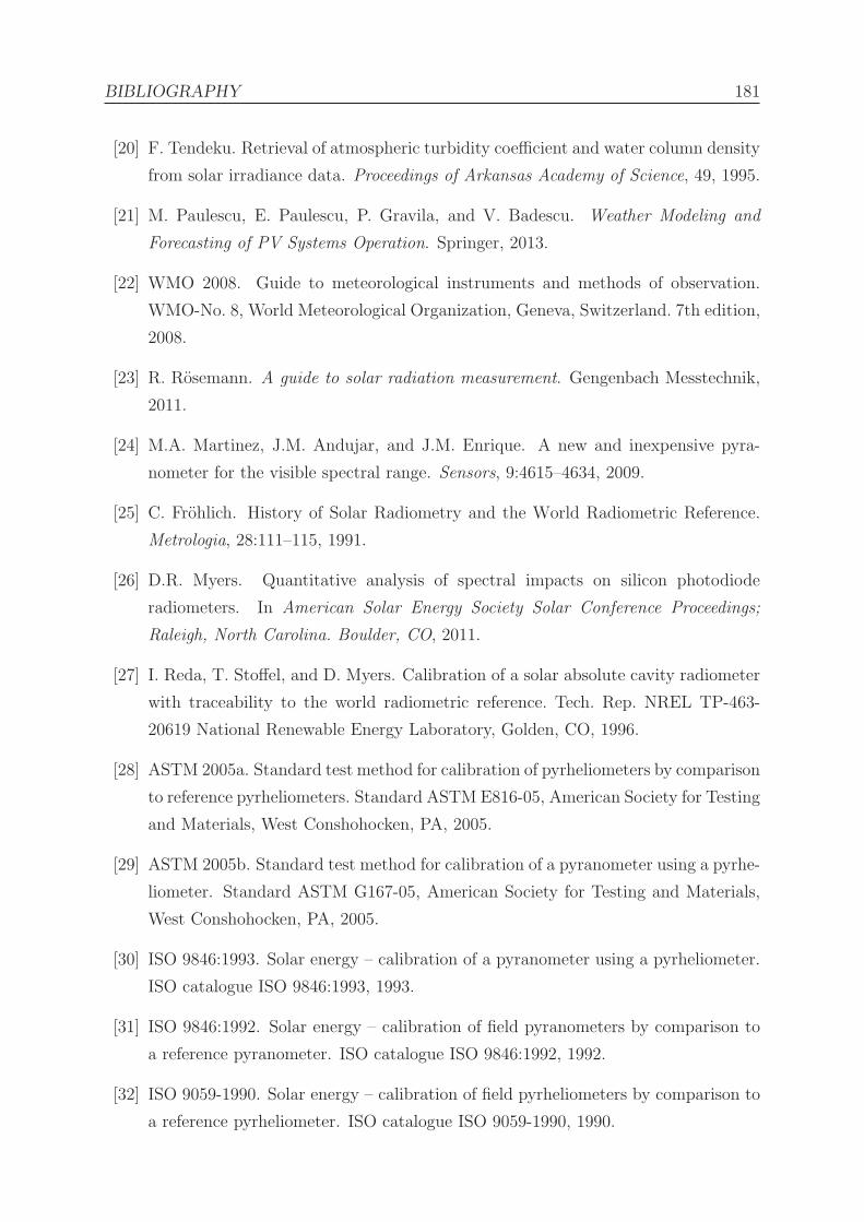
BIBLIOGRAPHY 181
[20] F. Tendeku. Retrieval of atmospheric turbidity coefficient and water column density
from solar irradiance data. Proceedings of Arkansas Academy of Science, 49, 1995.
[21] M. Paulescu, E. Paulescu, P. Gravila, and V. Badescu. Weather Modeling and
Forecasting of PV Systems Operation. Springer, 2013.
[22] WMO 2008. Guide to meteorological instruments and methods of observation.
WMO-No. 8, World Meteorological Organization, Geneva, Switzerland. 7th edition,
2008.
[23] R. Rosemann. A guide to solar radiation measurement. Gengenbach Messtechnik,
2011.
[24] M.A. Martinez, J.M. Andujar, and J.M. Enrique. A new and inexpensive pyra-
nometer for the visible spectral range. Sensors, 9:4615–4634, 2009.
[25] C. Frohlich. History of Solar Radiometry and the World Radiometric Reference.
Metrologia, 28:111–115, 1991.
[26] D.R. Myers. Quantitative analysis of spectral impacts on silicon photodiode
radiometers. In American Solar Energy Society Solar Conference Proceedings;
Raleigh, North Carolina. Boulder, CO, 2011.
[27] I. Reda, T. Stoffel, and D. Myers. Calibration of a solar absolute cavity radiometer
with traceability to the world radiometric reference. Tech. Rep. NREL TP-463-
20619 National Renewable Energy Laboratory, Golden, CO, 1996.
[28] ASTM 2005a. Standard test method for calibration of pyrheliometers by comparison
to reference pyrheliometers. Standard ASTM E816-05, American Society for Testing
and Materials, West Conshohocken, PA, 2005.
[29] ASTM 2005b. Standard test method for calibration of a pyranometer using a pyrhe-
liometer. Standard ASTM G167-05, American Society for Testing and Materials,
West Conshohocken, PA, 2005.
[30] ISO 9846:1993. Solar energy – calibration of a pyranometer using a pyrheliometer.
ISO catalogue ISO 9846:1993, 1993.
[31] ISO 9846:1992. Solar energy – calibration of field pyranometers by comparison to
a reference pyranometer. ISO catalogue ISO 9846:1992, 1992.
[32] ISO 9059-1990. Solar energy – calibration of field pyrheliometers by comparison to
a reference pyrheliometer. ISO catalogue ISO 9059-1990, 1990.

182 BIBLIOGRAPHY
[33] ISO 9060-1990. Solar energy – specification and classification of instruments for
measuring hemispherical solar and direct solar radiation. ISO catalogue, ISO 9060-
1990, 1990.
[34] S. Cros and L. Wald. Survey of the main databases providing solar radiation data
at the ground level. In 23rd EARSeL Annual Symposium “Remote Sensing in
Transition”, Ghent, Belgium, 2003.
[35] G. Konig-Langlo, R. Sieger, H. Schmithusen, A. Bucker, F. Richter, and E.G.
Dutton. The Baseline Surface Radiation Network and its World Radiation Mon-
itoring Centre at the Alfred Wegener Institute. WMO WCRP-24/2013. http:
//www.bsrn.awi.de/, 2013. Last accessed April 2015.
[36] WRDC. http://wrdc-mgo.nrel.gov/, 1964. Last accessed April 2015.
[37] A.S. Angstrom. Solar and terrestrial radiation. Q. J. Roy. Met. Soc., 50:126, 1924.
[38] A.K. Katiyar and C.K. Pandey. A review of solar radiation models, Part I. Journal
of Renewable Energy, 2013, 2013. 10.1155/2013/168048.
[39] C.A. Gueymard, P. Jindra, and V. Estrada-Cajigal. A critical look at recent in-
terpretations of the Angstrom approach and its future in global solar radiation
prediction. Solar Energy, 54:357–363, 1995.
[40] J. Almorox. Estimating global solar radiation from common meteorological data in
aranjuez, spain. Turk. J. Phys., 35:53–64, 2011.
[41] J.M. Gordon and M. Hochman. On correlations between beam and global radiation.
Solar Energy, 32:329–336, 1984.
[42] G.F. Orgil and K.G. Hollands. Correlation equation for hourly diffuse radiation on
a horizontal surface. Solar Energy, 19:357–359, 1977.
[43] D.G. Erbs, S.A. Klein, and J.A. Duffie. Estimation of the diffuse radiation fraction
for hourly, daily, and monthly-average global radiation. Solar Energy, 28:293, 1982.
[44] D.T. Reindl, W.A. Beckmann, and J.A. Duffie. Diffuse fraction correlations. Solar
Energy, 45(1):1–7, 1990.
[45] E.L. Maxwell. A quasi-physical model for converting hourly global horizontal to
direct normal insolation. Technical Report No. SERI/TR-215-3087, Golden, CO:
Solar Energy Research Institute, 1987.

BIBLIOGRAPHY 183
[46] P. Ineichen. Comparison and validation of three global-to-beam irradiance models
against ground measurements. Solar Energy, 82:501–512, 2008.
[47] C.A. Gueymard. Direct solar transmittance and irradiance predictions with broad-
band models. Part I: detailed theoretical performance. Solar Energy, 74:355–379,
2003.
[48] F. Vignola, J. Michalsky, and T. Stoffel. Solar and Infrared Radiation Measure-
ments. CRC Press, 2012.
[49] M.A. Behrang, E. Assareh, A. Ghanbarzadeh, and A.R. Noghrehabadi. The po-
tential of different artificial neural network (ANN) techniques in daily global solar
radiation modeling based on meteorological data. Solar Energy, 84:1468–1480, 2010.
[50] J. Mubiru and E.J.K.B. Banda. Estimation of monthly average daily global solar
irradiation using artificial neural networks. Solar Energy, 82:181–187, 2008.
[51] A. Linares-Rodriguez, J.A. Ruiz-Arias, D. Pozo-Vazquez, and J. Tovar-Pescador.
An artificial neural network ensemble model for estimating global solar radiation
from meteosat satellite images. Energy, 61:636–645, 2013.
[52] Y. Eissa, P.R. Marpu, I. Gherboudj, H. Ghedira, T.B.M.J. Ouarda, and M. Chiesa.
Artificial neural network based model for retrieval of the direct normal, diffuse
horizontal and global horizontal irradiances using SEVIRI images. Solar Energy,
89:1–16, 2013.
[53] D. Cano, J.M. Monget, H. Guillard, M. Albuisson, N. Regas, and L. Wald. A
method for the determination of the global solar radiation from meteorological
satellite data. Solar Energy, 37:31–39, 1986.
[54] R. Perez, P. Ineichen, K. Moore, C. Chain, M. Kmiecik, R. George, and F. Vignola.
A new operational satellite to irradiance model: description and validation. Solar
Energy, 73(5):307–317, 2002.
[55] C. Rigollier, M. Lefevre, and L. Wald. The method Heliosat-2 for deriving shortwave
solar radiation from satellite images. Solar Energy, 77:159–169, 2004.
[56] A. Zelenka, R. Perez, R. Seals, and D. Renne. Effective accuracy of the satellite-
derived hourly irradiance. Theor Appl Climatol, 62:199–207, 1999.
[57] K. Yang, G.W. Huang, and N. Tamaig. A hybrid model for estimating global solar
radiation. Solar Energy, 70(1):13–22, 2001.

184 BIBLIOGRAPHY
[58] K.G. Karlsson, A. Riihel, R. Muller, J.F. Meirink, J. Sedlar, M. Stengel, M. Lock-
hoff, J. Trentmann, F. Kaspar, R. Hollmann, and E. Wolters. CLARA-A1: a cloud,
albedo, and radiation dataset from 28 yr of global AVHRR data. Atmos. Chem.
Phys., 13:5351–5367, 2013.
[59] J. Polo, L.F. Zarzalejo, and L. Ramırez. Solar radiation derived from satellite
images. In M. Paulescu, E. Paulescu, P. Gravila, and V. Badescu, editors, Weather
Modeling and Forecasting of PV Systems Operation. Springer, 2013.
[60] L. Diabate, H. Demarcq, N. Michaud-Regas, and L. Wald. Estimating incident
solar radiation at the surface from images of the Earth transmitted by geostationary
satellites: the Heliosat project. International Journal of Solar Energy, 5:261–278,
1988a.
[61] C. Rigollier, O. Bauer, and L. Wald. On the clear sky model of the ESRA – Eu-
ropean Solar Radiation Atlas – with respect to the heliosat method. Solar Energy,
68:33–48, 2000.
[62] L. Wald. Heliosat-4 use of ground albedo and MSG parameters. MACC-II Deliv-
erable D 123.3, 2014.
[63] C. Schillings, H. Mannstein, and R. Meyer. Operational method for deriving high
resolution direct normal irradiance from satellite data. Solar Energy, 76:475–484,
2004.
[64] IEA/SHC task 36. Solar resource knowledge management, IEA/SHC task 36. In-
ternational Energy Agency Solar Heating and Cooling Programme.
[65] M. Suri and T. Cebecauer. SolarGIS: New web-based service offering solar radiation
data and PV simulation tools for Europe, North Africa and Middle East. In EU-
ROSUN 2010 Conference, Graz, Austria, 2010. http://www.geomodelsolar.eu.
Last accessed April 2015.
[66] P. Blanc, B. Gschwind, M. Lefevre, and L. Wald. The HelioClim project: Surface
solar irrradiance data for climate applications. Remote Sensing, 3:343–361, 2011.
http://www.helioclim.org. Last accessed April 2015.
[67] Irsolav. http://irsolav.com/, 2015. Last accessed April 2015.
[68] 3Tier. http://www.3tier.com/en/, 2015. Last accessed April 2015.
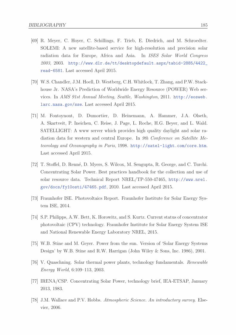
BIBLIOGRAPHY 185
[69] R. Meyer, C. Hoyer, C. Schillings, F. Trieb, E. Diedrich, and M. Schroedter.
SOLEMI: A new satellite-based service for high-resolution and precision solar
radiation data for Europe, Africa and Asia. In ISES Solar World Congress
2003, 2003. http://www.dlr.de/tt/desktopdefault.aspx/tabid-2885/4422_
read-6581. Last accessed April 2015.
[70] W.S. Chandler, J.M. Hoell, D. Westberg, C.H. Whitlock, T. Zhang, and P.W. Stack-
house Jr. NASA’s Prediction of Worldwide Energy Resource (POWER) Web ser-
vices. In AMS 91st Annual Meeting, Seattle, Washington, 2011. http://eosweb.
larc.nasa.gov/sse. Last accessed April 2015.
[71] M. Fontoynont, D. Dumortier, D. Heinemann, A. Hammer, J.A. Olseth,
A. Skartveit, P. Ineichen, C. Reise, J. Page, L. Roche, H.G. Beyer, and L. Wald.
SATELLIGHT: A www server which provides high quality daylight and solar ra-
diation data for western and central Europe. In 9th Conference on Satellite Me-
teorology and Oceanography in Paris, 1998. http://satel-light.com/core.htm.
Last accessed April 2015.
[72] T. Stoffel, D. Renne, D. Myers, S. Wilcox, M. Sengupta, R. George, and C. Turchi.
Concentrating Solar Power. Best practices handbook for the collection and use of
solar resource data. Technical Report NREL/TP-550-47465, http://www.nrel.
gov/docs/fy10osti/47465.pdf, 2010. Last accessed April 2015.
[73] Fraunhofer ISE. Photovoltaics Report. Fraunhofer Institute for Solar Energy Sys-
tem ISE, 2014.
[74] S.P. Philipps, A.W. Bett, K. Horowitz, and S. Kurtz. Current status of concentrator
photovoltaic (CPV) technology. Fraunhofer Institute for Solar Energy System ISE
and National Renewable Energy Laboratory NREL, 2015.
[75] W.B. Stine and M. Geyer. Power from the sun. Version of ‘Solar Energy Systems
Design’ by W.B. Stine and R.W. Harrigan (John Wiley & Sons, Inc. 1986), 2001.
[76] V. Quaschning. Solar thermal power plants, technology fundamentals. Renewable
Energy World, 6:109–113, 2003.
[77] IRENA/CSP. Concentrating Solar Power, technology brief, IEA-ETSAP, January
2013, 1983.
[78] J.M. Wallace and P.V. Hobbs. Atmospheric Science. An introductory survey. Else-
vier, 2006.

186 BIBLIOGRAPHY
[79] R.B. Stull. An Introduction to Boundary Layer Meteorology. Kluwer Academic
Publishers. Springer, 1988.
[80] J.C. Kaimal and J.J. Finnigan. Atmospheric boundary layer flows: their structure
and measurement. Oxford University Press, New York, NY, 1994.
[81] W. Jiang, X. Yumao, and Y. Hongbin. Base of Boundary-layer Meteorology. Nan-
jing: Nanjing University Press, 1994.
[82] J.R. Garratt. The Atmospheric Boundary Layer. Cambridge University Press,
Cambridge, 1992.
[83] T.F. Stocker, D. Qin, G.K. Plattner, M. Tignor, S.K. Allen, J. Boschung, A. Nauels,
Y. Xia, V. Bex, and P.M. Midgley. IPCC, 2013: Climate Change 2013: The
Physical Science Basis, volume 29. Cambridge University Press, Cambridge, United
Kingdom and New York, NY, USA, 2013.
[84] W.C. Hinds. Aerosol Technology. Properties, Behavior, and Measurement of Air-
borne Particles. John Wiley & Sons, Inc., 1999.
[85] R. Jaenicke. Atmospheric aerosol size distribution. In R.M. Harrison, editor, At-
mospheric Particles, pages 543–596. John Wiley & Sons, Inc., 1998.
[86] C. Weitkamp. Lidar, Range-Resolved Optical Remote Sensing of the Atmosphere.
Springer, 2005.
[87] K.Y. Kondtratyev. Climatic effects of Aerosol and Clouds. Springer, 1999.
[88] I. Tegen and A.A. Lacis. Modeling of particle size distribution and its influence on
the radiative properties of mineral dust aerosol. J. Geophys. Res., 101(19):237–244,
1996.
[89] F. Li, A.M. Vogelmann, and V. Ramanathan. Saharan dust aerosol radiative forcing
measured from space. Journal of Climate, 17(13):2558–2571, 2004.
[90] N. Bellouin, O. Boucher, J. Haywood, and M.S. Reddy. Global estimate of aerosol
direct radiative forcing from satellite measurements. Nature, 438:1138–1141, 2005.
[91] J. Zhang, S.A. Christopher, L.A. Remer, and Y.J. Kaufman. Shortwave aerosol
cloud-free radiative forcing from Terra II: Seasonal and global distributions. J.
Geophys. Res, 110, 2005.

BIBLIOGRAPHY 187
[92] F. Marenco, V. Santacesaria, A.F. Bais, D. Balis, A. di Sarra, A. Papayannis, and
C. Zerefos. Optical properties of tropospheric aerosols determined by lidar and
spectrophotometric measurements (Photochemical Activity and Solar Ultraviolet
Radiation Campaign). Appl. Opt., 36(27):6875–6886, 1997.
[93] E.J. Welton, K.J. Voss, P.K. Quinn, P.J. Flatau, K. Markowicz, J.R. Campbell,
J.D. Spinhirne, H.R. Gordon, and J.E. Johnson. Measurements of aerosol vertical
profiles and optical properties during INDOEX 1999 using micropulse lidars. J.
Geophys. Res., 107:8019–8039, 2002.
[94] M.I. Mishchenko, L.D. Travis, and A.A. Lacis. Scattering, Absorption and Emission
of Light by Small Particles. Cambridge University Press, 2002.
[95] C.F. Bohren and D.R. Huffman. Absorption and Scattering of Light by Small Par-
ticles. John Wiley & Sons, Inc., 1983.
[96] H.C. van de Hulst. Light scattering by small particles. Dover Publications, Inc.,
1981.
[97] G. Mie. Beitrage zur Optik truber Medien, speziell kolloidaler Metallosungen. An-
nalen der Physik, 330(3):377–445, 1908.
[98] M.I. Mishchenko. Calculation of the amplitude matrix for a nonspherical particle
in a fixed orientation. Appl. Opt., 39:1026–1031, 2000.
[99] E.M. Purcell and C.R. Pennypacker. Scattering and absorption of light by non-
spherical dielectric grains. Astrophysical Journal, 186:705–714, 1973.
[100] V. Kovalev and W. Eichinger. Elastic Lidar. Theory, Practice, and Analysis Meth-
ods. John Wiley & Sons, Inc., 2004.
[101] D.I. Cooper and W.E. Eichinger. Structure of the atmosphere in an urban planetary
boundary layer from lidar and radiosonde observations. Journal of Geophysical
Research, 99:22937–22948, 1994.
[102] B.A. Holmen, W.E. Eichinger, and R.G. Flocchini. Application of elastic lidar to
PM10 emissions from agricultural nonpoint sources. Environmental Science Tech-
nology, 32:3068–3076, 1998.
[103] C.A. Gueymard. Stable analytical inversion solution for processing lidar returns.
Applied Optics, 20(2), 1981.

188 BIBLIOGRAPHY
[104] British Petroleum Company. BP Statistical Review of World Energy June 2014,
63 edition. London, British Petroleum Co., 2014.
[105] The World Bank. CO2 emissions (metric tons per capita). Technical report, World
Development Indicators, 2014.
[106] Kahramaa. Statistics report 2012. Technical report, Qatar General Electricity and
Water Corporation KAHRAMAA, Corporate Planning and Business development,
2013.
[107] QNV 2030. Qatar National Vision 2030. Technical report, General Secretariat For
Development Planning, 2008.
[108] Pan-Arab renewable energy strategy 2030, roadmap of actions for implementation.
IRENA, 2014.
[109] Supreme Committee. Qatar Foundation stadium. http://www.sc.qa/en/
stadiums/qatar-foundation-stadium. Last accessed April 2015.
[110] M.M. Haruni. The solar pilot project in Qatar. Solar and Wind Technology, 1(2):93–
108, 1984.
[111] Qatar Foundation Magazine. The Foundation, issue 73, January 2015. Qatar
Foundation, Doha, Qatar, 2015.
[112] Total. A new energy future with solar energy. Total Marketing services, New
Energies, Paris, France, 2013.
[113] N. May. Eco-balance of a Solar Electricity Transmission from North Africa to
Europe. PhD thesis, Technical University Of Braunschweig, Faculty for Physics
and Geological Sciences, 2005.
[114] J. Betak, M. Suri, T. Cebecauer, and A. Skoczek. Solar resource and photovoltaic
electricity potential in EU-MENA region. In EUPVSEC2012 Conference, 2012.
[115] Concentrating solar power for the Mediterranean region, final report. Institute of
Technical Thermodynamics, Sections system analysis and technology assessment,
DLR, 2005.
[116] Feasibility study on combined CSP-seawater desalination technology. 6th World
Water Forum, Marseille, France, 2012.

BIBLIOGRAPHY 189
[117] High-quality renewable energy resource data for the Kingdom of Saudi Arabia.
King Abdullah City for Atomic and Renewable Energy (K.A.CARE), Renewable
Resource Monitoring and Mapping (RRMM) Program, 2013.
[118] The UAE solar atlas. The Research Center for Renewable Enregy Mapping and
Assessment (ReCREMA), Masdar Institute, 2013.
[119] D. Bachour and D. Perez-Astudillo. Ground-measurement GHI map for Qatar.
Energy Procedia, 49:2297–2302, 2014. Proceedings of the SolarPACES 2013 Inter-
national Conference.
[120] S. Emeis and K. Schafer. Remote sensing methods to investigate boundary-layer
structures relevant to air pollution in cities. Bound.-Lay. Meteorol., 121:377–385,
2006.
[121] C. Munkel, S. Emeis, and K. Schafer. Aerosol concentration measurements with a
lidar ceilometer: results of a one year measuring campaign. Proc. SPIE 5235, pages
486–496, 2004.
[122] C. Munkel. Boundary layer and air quality monitoring with a commercial lidar
ceilometer. Proc. SPIE 6367, 2006.
[123] C. Munkel, K. Schafer, and S. Emeis. Investigation of boundary layer dynamics,
dust and volcanic ash clouds with laser ceilometer. Proc. SPIE 8890, Remote Sens-
ing of Clouds and the Atmosphere XVIII; and Optics in Atmospheric Propagation
and Adaptive Systems XVI, 2013.
[124] R.C. Munoz and R.I. Alcafuz. Variability of urban aerosols over Santiago, Chile:
Comparison of surface PM10 concentrations and remote sensing with ceilometer
and lidar. Aerosol and Air Quality Research, 12:8–19, 2012.
[125] C. Munkel and J. Rasanen. New optical concept for commercial lidar ceilometers
scanning the boundary layer. Proc. SPIE 5571, pages 364–374, 2006.
[126] V.R. Morris. Vaisala ceilometer (VCEIL) handbook. U.S. Department of Energy,
Office of Science, Office of Biological and Environmental Research, Atmospheric
Research, 2012.
[127] C. Munkel. Mixing height determination with lidar ceilometers – results from
Helsinki Testbed. Meteorol. Z., pages 451–459, 2007.
190 BIBLIOGRAPHY
[128] C. Munkel. Automatic monitoring of boundary layer structures with ceilometer.
WMO Technical Conference on Meteorological and Environmental Instruments and
Methods of Observation, Helsinki, Finland, pages 2–17, 2010.
[129] D. Bachour and D. Perez-Astudillo. Boundary layer height measurements over Doha
using lidar. Energy Procedia, 57:1086–1091, 2014. Proceedings of the SolarPACES
2013 International Conference.
[130] J.J. Michalsky. The astronomical almanac’s algorithm for approximate solar posi-
tion (1950-2050). Solar Energy, 40:227–235, 1988.
[131] I. Moradi. Quality control of global solar radiation using sunshine duration hours.
Energy, 34:1–6, 2009.
[132] S. Younes, R. Claywell, and T. Muneer. Quality control of solar radiation data:
present status and proposed new approaches. Energy, 30:1533–1549, 2005.
[133] T. Muneer and F. Fairooz. Quality control of solar radiation and sunshine mea-
surements – lessons learnt from processing worldwide databases. Building Services
Eng. Res. Technol., 23:151–166, 2002.
[134] W. Tang, K. Yang, J. He, and J. Qin. Quality control and estimation of global
solar radiation in China. Solar Energy, 84:466–475, 2010.
[135] M. Journee and C. Bertrand. Quality control of solar radiation data within the
RMIB solar measurements network. Solar Energy, 85:72–86, 2011.
[136] G. Maxwell, S. Wilcox, and M. Rymes. User’s manual for SERI QC software –
Assessing the quality of solar radiation data. NREL/TP-463-5608, National Re-
newable Energy Laboratory, Golden, Colorado, 1993.
[137] C.N. Long and E.G. Dutton. BSRN global network recommended QC tests, v2.0.
Technical report, BSRN Technical Report, 2002.
[138] B. Espinar, B. Gschwind, L. Wald, and C. Thomas. An OGC web processing service
for assessing the quality of solar radiation measurements. 27th International Con-
ference on Informatics for Environmental Protection, Hamburg, Germany, 2013.
[139] F. Vejen, C. Jacobsson, U. Fredriksson, M. Moe, L. Andresen, E. Hellsten, P. Rissa-
nen, T. Palsdottir, and T. Arason. Quality control of meteorological observations.
Automatic methods used in the Nordic countries. Norwegian Meteorological Insti-
tute, 2002.

BIBLIOGRAPHY 191
[140] P. Ineichen. Global irradiation: average and typical year, and year to year an-
nual variability. Research report of the Institut of the Environnemental Sciences,
University of Geneva, 2011.
[141] S. Lohmann, C. Schillings, B. Mayer, and R. Meyer. Long-term variability of
solar direct and global radiation derived from ISCCP data and comparison with
reanalysis data. Sol Energy, 80:1390–1401, 2006.
[142] D.H.W. Li and J.C. Lam. An analysis of climatic parameters and sky condition
classification. Building and Environment, 36(4):435–445, 2001.
[143] J. Calbo, J.A. Gonzalez, and D. Pages. A method for sky condition classification
from ground-based solar radiation measurements. J Appl Meteorol, 40:2193–2199,
2001.
[144] K. Scharmer and J. Greif. The European Solar Radiation Atlas. Les Presses de
l’Ecole des Mines, Paris, 2000. (1:24).
[145] M.D. Islam, I. Kubo, M. Ohadi, and A.A. Alili. Measurement of solar energy
radiation in Abu Dhabi, UAE. Applied Energy, 86:511–515, 2009.
[146] NOAA. http://www.esrl.noaa.gov/gmd/grad/solcalc/. Last accessed April
2015.
[147] R.W. Reynolds and T.M Smith. Improved global sea-surface temperature analysis
using optimum interpolation. J Climate, 7:929–948, 1994.
[148] T.M. Smith, R.W. Reynolds, R.E. Livezey, and D.C. Stokes. Reconstruction of
historical sea-surface temperatures using empirical orthogonal functions. J Climate,
9:1403–1420, 1996.
[149] R. Mendelssohn, F.B. Schwing, and S.J. Bograd. Spatial structure of subsurface
temperature variability in the California Current. J. Geophys Res, 108(C3):3093,
2003.
[150] D. Kondrashov and M. Ghil. Spatio-temporal filling of missing points in geophysical
data sets. Nonlin Processes Geophys, 13:151–159, 2006.
[151] E.L. Maxwell. Final Technical Report, National Solar Radiation Data Base (1961-
1990), NREL/TP-463-5784 DE9500262, 1995. National Renewable Energy Labo-
ratory. Golden, Colorado, USA.

192 BIBLIOGRAPHY
[152] A. Kumar, S. Gomathinayagam, G. Giridhar, I. Mitra, R. Vashistha, R. Meyer,
M. Schwandt, and K. Chhatbar. Field experiences with the operation of solar
radiation resource assessment stations in India. In Energy Procedia, Proceedings of
the SolarPACES International Conference, volume 49, pages 2351–2361, 2013.
[153] G. Vijayakumar, S.A. Klein, and W.A. Beckman. Analysis of short-term solar
radiation data. Solar Energy, 79(5):495–504, 2005.
[154] R.E. Carrillo, T.C. Aysal, and K.E. Barner. A generalized Cauchy distribution
framework for problems requiring robust behavior. EURASIP Journal on Advances
in Signal Processing, 2010:312989, 2010.
[155] R. Meyer, C. Gueymard, and P. Ineichen. Standardizing and benchmarking of mod-
eled DNI data products. In Proceedings of SolarPACES International Conference,
2011.
[156] M. Suri, J. Remund, T. Cebecauer, C. Hoyer-Klick, D. Dumortier, T. Huld,
P.W. Stackhouse Jr., and P. Ineichen. Comparison of direct normal irradiation
maps for Europe. In Proc SolarPACES Conf Berlin, Germany, 2009.
[157] W.D. Collins, P.J. Rasch, B.E. Eaton, B.V. Khattatov, J.-F. Lamarque, and C.S.
Zender. Simulating aerosols using a chemical transport model with assimilation
of satellite aerosol retrievals: Methodology for INDOEX. J Geophysical Research:
Atmospheres, 106(D7):7313–7336, 2001.
[158] CLVIEW. http://www.vaisala.com/en/products/ceilometers/Pages/
CL-VIEW.aspx, 2015. Last accessed April 2015.
[159] C.D. Papadimas, N. Hatzianastassiou, C. Matsoukas, M. Kanakidou, N. Mihalopou-
los, and I. Vardavas. The direct effect of aerosols on solar radiation over the broader
Mediterranean basin. Atmos Chem Phys, 12:7165–7185, 2012.
[160] V. Ramanathan, P.J. Crutzen, J.T. Kiehl, and D. Rosenfeld. Aerosol, climate and
the hydrological cycle. Science, 294:2119–2124, 2001.
[161] N. Hatzianastassiou, C. Matsoukas, E. Drakakis, P.W. Stackhouse Jr., P. Koepke,
A. Fotiadi, K.G. Pavlakis, and I. Vardavas. The direct effect of aerosols on solar
radiation based on satellite observations, reanalysis datasets, and spectral aerosol
optical properties from Global Aerosol Data Set (GADS). Atmos Chem Phys,
7:2585–2599, 2007.

BIBLIOGRAPHY 193
[162] M. Lefevre, A. Oumbe, P. Blanc, B. Espinar, B. Gschwind, Z. Qu, L. Wald,
M. Schroedter-Homscheidt, C. Hoyer-Klick, A. Arola, A. Benedetti, J.W. Kaiser,
and J.-J. Morcrette. McClear: a new model estimating downwelling solar radiation
at ground level in clear-sky conditions. Atmos. Meas. Tech., 6:2403–2418, 2013.
[163] T. Cebecauer and M. Suri. Accuracy improvements of satellite-derived solar re-
source based on GEMS re-analysis aerosols. In Proc. Conf. SolarPACES 2010,
Perpignan, France, 2010.
[164] GeoModel. http://www.geomodelsolar.eu/_docs/various/SolarGIS_
validation_SaudiArabia_2013-02.pdf, 2013. Technical report. Last accessed
April 2015.
[165] C.N. Long and T.P. Ackerman. Identification of clear skies from broadband pyra-
nometer measurements and calculation of downwelling shortwave cloud effects.
Journal of Geophysical Research, 105 (D12):15609–15626, 2000.
[166] R. Perez and P. Ineichen. Making full use of the clearness index for parameterizing
hourly insolation conditions. Solar Energy, 45(2):111–114, 1990.


![arXiv:1408.4805v2 [astro-ph.HE] 10 Oct 2014 · ... O. Martinez14, J. Mart´ınez ... Universidad Nacional Aut´onoma de M´exico, Mexico D ... 25 Universidad Aut´onoma del Estado](https://img.dokumen.tips/doc/110x75/5ac080937f8b9ac6688c3eff/arxiv14084805v2-astro-phhe-10-oct-2014-o-martinez14-j-martinez-.jpg)