Embed Size (px)
Citation preview

UNIVERSITA’ DEGLI STUDI DI ROMA
“ LA SAPIENZA”
FACOLTA’ DI INGEGNERIA ELETTRONICA
DIPARTIMENTO DI ENERGETICA
XVIII CICLO DI DOTTORATO DI RICERCA IN ELETTROMAGNETISMO
TRIENNIO ACCADEMICO 2003-2005
CLASSICAL AND QUANTUM APPROACH OF QUASI NORMAL MODES
IN LINEAR OPTICAL REGIME: AN APPLICATION TO
ONE DIMENSIONAL PHOTONIC CRYSTALS
Coordinatore Relatore Chiarmo Prof. Gerosa Giorgio Chiarmo Prof. Bertolotti Mario Dottorando Sigla di catalogazione: Dott. Ing. Settimi Alessandro ING/INF-02

1
2
In memoria di mio padre
Franco,
detto “Schizza” ed anche “Pico della Mirandola”.

3

4
INDEX
Introduction. 10
First Part: QNM’s approach for open cavities in classical electrodynamics. 16
Chapter 1: Quasi Normal Mode’s approach for open cavities. 1. Introductive outlines. 17
1. 1. QNM’s literature. 18
2. Closed and open system. 19
2. 1. Comparison of QNM’s with other expansions. 22
3. QNM’s linear space. 24
3. 1. Linear space. 24
3. 2. Inner product. 25
3. 3. Operators on linear space. 25
3. 4. Self-adjoint operators. 26
3. 5. Eigen frequencies and functions. 26
3. 6. Damped harmonic oscillator. 27
4. QNMs of a linear Fabry-Perot cavity. 28
5. Discussion and conclusions. 30
References. 31
Figure and caption. 32
Chapter 2: QNM’s approach for open cavities
in absence of external pumping:
an application to one dimensional Photonic Crystals. 1. Introduction. 33
2. Examining deeper QNM’s approach. 34
3. Completeness of QNM’s representation inside 1D-PC cavities. 37
4. QNM’s frequencies for 1D-PBG structures. 40

5
5. Conclusions. 42
Appendix A. 42
References. 45
Figures and captions. 47
Chapter 3: QNM’s approach for open cavities
excited by an external pumping:
Transmission properties of a 1D-PBG structure. 1. Introduction. 51
2. Extending QNM’s approach:
e.m. problem of an open cavity excited by an external pump. 52
3. An application of QNM’s approach:
Transmission properties of a symmetric QW 1D-PBG structure. 54
3. 1. QNM’s frequencies and transmission resonances. 55
3. 2. QNM’s functions and transmission peaks. 56
3. 3. 1D-PBG structures excited by two counter-propagating field pumps. 57
4. Conclusions. 59
Appendix B. 60
References. 61
Figures and captions. 62
Second Part: QNM’s approach for open cavities in quantum electrodynamics. 69
Chapter 4: Non canonical Quasi Normal Mode’s Quantization for open cavities.
1. Introductive discussion. 70
2. Incoming wave conditions. 72
2. 1. Extending QNM’s approach:
e.m. problem of an open cavity excited
by two classical counter-propagating incoming waves. 73
3. Second quantization. 75
3. 1. Canonical commutation rules in free space:
quantum apparatus for counter-propagation of incoming waves. 76
3. 2. Non canonical QNM’s commutation rules in an open cavity:
link of QNM’s operators inside the cavity

6
with NM’s operators of the free space. 79
3. 3. Auto-correlation function of e.m. field inside an open cavity
as QNM’s superposition depending on the incoming waves. 82
4. Discussion and conclusions. 84
References. 85
Figures and captions. 86
Chapter 5: Density of probability for QNMs:
link with boundary conditions of open cavities.
1. Introduction. 88
2. Density of states. 90
2. 1. Frequencies of QNMs as resonances of DOS. 91
2. 2. DOS inside an open cavity:
link with the phase-difference
of two external counter-propagating laser-beams. 93
3. Discussion and conclusions. 96
Appendix C: Examining deeper the link of the LDOS
with the auto-correlation function of the e.m. field. 97
References. 100
Figures and captions. 102
Third Part: QNM’s approach for emission processes in open cavities. 104
Chapter 6: Spontaneous Emission and coherent control of Stimulated Emission
inside one dimensional Photonic Crystals (Weak Coupling regime).
1. Introduction. 105
2. Atomic emission power inside open cavities. 107
2. 1. Sensitivity function of dipole-e.m. field coupling. 109
3. Spontaneous emission inside a symmetric QW 1D-PBG. 110
4. Coherent control of stimulated emission inside a symmetric QW 1D-PBG. 113
5. Decay-times in units of dwell-times. 114
6. Discussion and conclusions. 117
Appendix D. Examining deeper the link of atomic emission power

7
with density of states (DOS). 117
References. 123
Figures and captions. 125
Chapter 7: Coherent Control of Stimulated Emission
inside 1D-PBG structures (Strong Coupling regime).
1. Introduction. 136
2. Coupling of an atom to an e.m. field. 137
2. 1. Quantum electrodynamics equations. 138
2. 2. Atom in the free space. 139
3. Atom inside an open cavity. 140
3. 1. Spontaneous emission: DOS corresponding to vacuum fluctuations. 140
3. 2. Stimulated emission:
DOS depending on the phase difference
of two counter-propagating laser-beams. 141
4. Emission probability of the atom. 142
4. 1. Strong coupling regime. 142
5. Emission spectrum of the atom. 144
5. 1. Poles of the emission spectrum. 146
6. Criteria to design an active delay line. 146
7. Conclusion. 151
References. 151
Figures and captions. 153
Discussion and conclusions. 162
8

9
INTRODUCTION
The definition of natural modes for confined structures is one of the central problems in
physics, as in nuclear physics, astrophysics, etc. The main problem is due to the boundary
conditions, when they are such to push out the problem from the class of Sturm-Liouville. This
occurs when boundary conditions imply the presence of eigen-values, as for example when a
scatterer excited from the outside gives rise to a transmitted and reflected field. An open cavity
with an external or internal excitation represents a “non-canonical “ problem, in the sense of a
Sturm–Liouville’s problem, due to the fact that cavity modes couple themselves with external
modes. This problem is crucial when one intends to study light-matter interaction effects as
absorption, spontaneous emission, stimulated emission, as they occur in micro-cavities.
Quasi Normal Mode’s (QNM’s) approach.
The problem of the field description inside an optical cavity which radiates outside has been
analyzed following several different points of view. The description of the e.m. field in an one side
open and homogeneous cavity has been discussed in terms of Quasi Normal Modes (QNMs) in ref.
[1]; the QNMs are defined inside a one dimensional leaky cavity, provided the open cavity is
defined by a discontinuity in the refractive index which must approach its constant asymptotic value
sufficiently rapidly.
In general, an optical cavity is not a conservative system, so the natural evolution of the e.m. field
can not be described by an hermitian operator and the treatment of the e.m. field in terms of Normal
Modes (NMs) has to be dropped. The QNM’s approach considers the realistic situation in which the
optical cavity is enclosed in an infinite external space. The lack of energy conservation for the open
cavity gives complex, instead of real, eigen frequencies. The evolution operator for the system is
not hermitian and the modes of the e.m. field are not Normal but Quasi Normal. In fact, under some
conditions over the refractive index: (a) the evolution of the QNMs is similar to the hermitian one
for the NMs, and (b) the e.m. field can be described as a superposition of QNMs only inside the
open cavity and the QNM’s functions form an orthogonal basis only according to a non-canonical
metrics. The QNM’s functions do not represent the e.m. field outside the cavity, while they
represent the “not stationary” modes into the cavity. For the reason of not being complete in the
whole space, they are called “Quasi-Normal” Modes.
Ho et al. in ref. [2] already made an essential first step towards the application of the QNMs
to quantum electrodynamics phenomema in one side open and homogeneous cavities: the second

10
quantization of the e.m. field in an open cavity is formulated, from first principles, in terms of the
QNMs, which are eigen-solutions of the evolution equation, decaying exponentially in time as
energy leaks to outside.
One dimensional (1D) Photonic Band Gap (PBG) structures.
One dimensional (1D) Photonic Band Gap (PBG) structures [3]-[5] of finite length manifest
all the aspects related to a class of problems which do not belong to the Sturm-Liouville’s class: in
fact, they behave as scattering objects when they are excited from outside and as open cavities when
excited from inside. These structures can be realized by a stack of dielectric layers arranged
according to some periodic or quasi-periodic sequence. Usually they are made alternating layers of
high and low index materials of suitable thickness. If the 1D-PBG structure is periodic it may be
thought as done by the superposition of a finite number of equal cells, each cell being usually
constructed by two materials. The essential property of these 1D-PBGs is the existence of allowed
and forbidden frequency bands and gaps, in analogy with energy bands and gaps of semiconductors.
At the same time, the distribution of the e.m. field intensity along the structure strongly changes by
changing the frequency or, in general if the e.m. field is coming from outside, the boundary
conditions.
In the wake of theoretical promulgation for 1D-PBGs, concern has turned to the question of
the behaviour of the atomic decay rate in such structures The density of states (DOS) is the
fundamental feature that determines the behaviour of the system ‘atom-field’ and characterizes the
various types of environments. The form and analytical properties of the DOS dictate the type of the
approximations permissible in formulating the equations governing the time evolution of the
system. When the DOS is a smooth function of frequency over the spectral range of atomic
transition, the rate of spontaneous and stimulated emission is described by the Fermi’s golden rule.
Abrupt changes in the DOS and photon localization effects may drastically modify the emission
dynamics. This modification takes the form of long time memory effects and non-Markovian
behaviour in the atom-reservoir interaction.
A substantial modification in the DOS can be effected by means of PBG structures. It has been
suggested that this would be accompanied by classical light localization, the inhibition of single-
photon emission, fractionalized single-atom inversion, a photon-atom bound state and anomalously
large vacuum Rabi’s splitting.

11
QNM’s approach for 1D-PBGs.
In the period of three years, required for the Ph-D course in Electromagnetism, some papers
have been published and recently submitted in order to extend the QNM’s treatment for the
description of the e.m. field inside 1D-PBGs. In ref. [6], a discussion is presented about the
completeness of the QNM’s representation and, moreover, a discussion on the complex frequencies,
as well as the corresponding field distributions. In a submitted paper [7], the role of the QNM’s
frequencies in the transmission coefficient is clarified; an application is performed for a symmetric
quarter wave structure.
The second quantization based on the QNM’s treatment has been extended to 1D-PBG
structures. In ref. [8], starting from this representation, the Feynman’s propagator is introduced to
calculate the decay rate of a dipole inside a 1D-PBG, in presence of vacuum fluctuations outside the
structure.
In a submitted paper [9], applying the second quantization for QNMs, the problem of counter-
propagation for two field pumps inside a 1D-PBG structure is discussed. The links between the
usual annihilation and creation operators, describing the two pumping fields, and the not canonical
QNM’s operators of a 1D-PBG are investigated; an application is performed for a symmetric
structure.
In ref. [10], the QNM’s second quantization is applied to discuss the quantum problem of an atom
embedded inside a 1D-PBG, pumped by two counter-propagating laser-beams. The e.m. field is
quantized in terms of the QNMs in the structure and the atom, modelled as a two-level system, is
assumed to be weakly coupled to just one of the QNMs.
In a paper to be submitted [11], the stimulated emission is discussed, in strong coupling regime, for
an atom embedded inside a 1D-PBG structure which is pumped by two counter-propagating laser
beams. Quantum electro-dynamics is applied to model the atom-e.m. field coupling, by considering
the atom as a two level system, the e.m. field as a superposition of normal modes, the coupling in
dipole approximation, and the equations of motion in Wigner-Weisskopf’s and rotating wave
approximations. Besides, the QNM’s quantization is adopted for the 1D-PBG, interpreting the local
density of states (LDOS) as the local density of probability to excite one QNM of the structure;
therefore, this LDOS depends on the phase difference of the two laser beams.
The present Ph-D thesis re-organizes the contents of the papers [6]-[11] in a systematic form,
examining the QNM’s approach for 1D-PBG structures still more thoroughly. This Ph-D thesis is
subdivided in three parts and consists of seven chapters. The first part, concerning the QNM’s
approach for open cavities in classical electrodynamics, consists of three chapters. Chapter 1 is
12
entitled “Quasi Normal Mode’s (QNM’s) approach for open cavities”. Chapter 2 is “QNM’s
approach for open cavities in absence of external pumping: an application to one dimensional (1D)
Photonic Crystals (PCs)”. Chapter 3, “QNM’s approach for open cavities excited by an external
pumping: Transmission properties of a 1D-PBG structure”. The second part, concerning the
QNM’s approach for open cavities in quantum electrodynamics, consists of two chapters. Chapter 4
is entitled “Non canonical QNM’ Quantization for open cavities”. Chapter 5 is “Density of
probability for QNMs: link with boundary conditions of open cavities”. The third part, concerning
the QNM’s approach for emission processes in open cavities, consists of two chapters. Chapter 6 is
entitled “Spontaneous Emission and coherent control of Stimulated Emission inside one
dimensional Photonic Crystals (Weak Coupling regime)”. Chapter 7, “Coherent Control of
Stimulated Emission inside 1D-PBG structures (Strong Coupling regime)”.
[1] P. T. Leung, S. Y. Liu, and K. Young, Phys. Rev. A 49, 3057 (1994); P. T. Leung, S. S. Tong,
and K. Young, J. Phys. A 30 2139 (1997); P. T. Leung, S. S. Tong, and K. Young, J. Phys. A 30,
2153 (1997); E. S. C. Ching, P. T. Leung, A. Maassen van der Brink, W. M. Suen, S. S. Tong, and
K. Young, Rev. Mod. Phys. 70, 1545 (1998); P. T. Leung, W. M. Suen, C. P. Sun and K. Young,
Phys. Rev. E 57, 6101 (1998).
[2] K. C. Ho, P. T. Leung, Alec Maassen van den Brink and K. Young, Phys. Rev. E 58, 2965
(1998).
[3] S. John, Phys. Rev. Lett. 53, 2169 (1984); S. John, Phys. Rev. Lett. 58, 2486 (1987); E.
Yablonovitch, Phys. Rev. Lett. 58, 2059 (1987); E. Yablonovitch and T. J. Gmitter, Phys. Rev.
Lett.. 63, 1950 (1989).
[4] J. Maddox, Nature (London) 348, 481 (1990); E. Yablonovitch and K.M. Lenny, Nature
(London) 351, 278, 1991; J. D. Joannopoulos, P. R. Villeneuve, and S. H. Fan, Nature (London)
386, 143 (1997).
[5] J. D. Joannopoulos, Photonic Crystals: Molding the Flow of Light (Princeton University Press,
Princeton, New York, 1995); K. Sakoda, Optical properties of photonic crystals (Springer Verlag,
Berlin, 2001); K. Inoue and K. Ohtaka, Photonic Crystals: Physics, Fabrication, and Applications
(Springer-Verlag, Berlin, 2004).
[6] A. Settimi, S. Severini, N. Mattiucci, C. Sibilia, M. Centini, G. D’Aguanno, M. Bertolotti, M.
Scalora, M. Bloemer, C. M. Bowden, Phys. Rev. E 68, 026614 (2003).
[7] S. Severini, A. Settimi, C. Sibilia, M. Bertolotti, A. Napoli, A. Messina, Quasi Normal
Frequencies in open cavities: an application to Photonic Crystals, in press on Acta Phys. Hung. B
(2006).

13
[8] S. Severini, A. Settimi, C. Sibilia, M. Bertolotti, A. Napoli, A. Messina, Phys. Rev. E 70,
056614 (2004).
[9] S. Severini, A. Settimi, C. Sibilia, M. Bertolotti, A. Napoli, A. Messina, Quantum counter-
propagation in open cavities via Quasi Normal Modes approach, submitted to Journal of Laser
Physics (2005).
[10] A. Settimi, S. Severini, C. Sibilia, M. Bertolotti, M. Centini, A. Napoli, N. Messina, Phys. Rev.
E 71, 066606 (2005).
[11] A. Settimi, S. Severini, C. Sibilia, M. Bertolotti, A. Napoli, A. Messina, Coherent Control of
stimulated emission inside one dimensional Photonic Crystals: strong coupling regime, to in press
on E.P.J. B (2006).
14

15
First Part:
QNM’s approach for open cavities in classical electrodynamics.

16
Chapter 1
Quasi Normal Mode’s approach for open cavities
1. Introductive outlines.
Resonators have the property to enhance the electromagnetic field in their interior, a property
which has many applications and makes them essential elements of most lasers [1].
In the radio-frequency and microwave range, resonators are usually closed cavities with dimensions
comparable with the wavelength. In the optical case at the beginning, it was neither possible nor
convenient to make cavities of dimensions comparable with the light wavelength. This precluded
the possibility of using closed resonators which are currently widely employed in the microwave
range and which actually represent a cavity with reflecting walls, because the number of low-loss
modes at optical frequencies would here be prohibitively large. To obtain a selection of the
oscillating modes, it was therefore necessary to make recourse to open side cavities. These open
resonators are without side walls and consist, in their simplest configuration, of two oppositely
mounted mirrors between which the active medium is placed. It is the geometry of the mirror
arrangement that accounts for radiation propagating in the preferred direction which, in its turn,
reduces dramatically the number of low-loss modes compared with closed resonators.
The first resonator configuration employed in optics was the Fabry-Perot interferometer consisting
of two parallel plane mirrors. One of them is partially transmitting to take out the generated
radiation. It is still one of the most widely used types of laser resonator. Its popularity stems not
only from its extreme simplicity, but also from the inherent possibility of obtaining high-energy
outputs.
Many years were spent in establishing the very existence of the modes, their specific features
in different resonators and the role played in their formation by the active medium, to learn whether
the modes close in losses are excited separately or simultaneously, and how all this affects the
characteristics of the laser radiation.
Underlying the theory of open resonators, like any other resonator devices, is the concept of
fundamental oscillations, or modes. By the resonator mode one understands a field distribution

17
whose dependence on time in the absence of external sources is described throughout the whole
volume by the same factor exp( )i tω− where ω is the fundamental circular frequency which, in the
general case, is complex: iω ω ω′ ′′= + , being ω′ and ω′′ real quantities. For empty resonators with
sources of loss 0ω′′ < , i.e. the oscillations die out in time while the shape of the spatial field
distribution remains unchanged.
The modes of an optical resonator can practically always be represented as a combination of several
light beams transforming into one another on reflection from the mirrors or interfaces, thus ensuring
reproducibility of the process in time. Thus the modes of the simplest linear resonators like the
plane resonator, which is still in use at present, consist of two spatially matched beams propagating
in opposite directions.
In this Ph-D thesis, only one-dimensional (1D) structures are considered. Several methods are
available to derive the electromagnetic field inside the structures together with transmission and
reflection coefficient. Two of these methods are the transfer matrix [1] and the ray method [2],
which can be applied to any kind of 1D structure with piecewise constant refractive index.
1. 1. QNM’s literature.
The definition of natural modes for confined structures is one of the central problems in
physics [4], as in nuclear physics, astrophysics, etc. The main problem is due to the boundary
conditions, when they are such to push out the problem from the class of Sturm-Liouville. This
occurs when boundary conditions imply the presence of eigen-values, as for example when a
scatterer excited from the outside [5] gives rise to a transmitted and reflected field. An open cavity
with an external or internal excitation represents a “non-canonical “ problem, in the sense of a
Sturm–Liouville’s problem, due to the fact that the cavity modes couple themselves with the
external modes. This problem is crucial when one intends to study light-matter interaction effects as
absorption, spontaneous emission, stimulated emission, as they occur in micro-cavities.
The problem of the field description inside an open cavity which radiates outside has been
discussed following several different points of view [6].
The description of the e.m. field in an one side open and homogeneous cavity has been discussed in
terms of Quasi Normal Modes (QNMs) in refs.
[1]; QNMs are discussed in a one dimensional leaky cavity, provided the cavity is defined by a
discontinuity in the refractive index which must approach its constant asymptotic value sufficiently
rapidly.
18
In general, an optical cavity is not a conservative system, so the natural evolution of the e.m. field
can not be described by an hermitian operator and the treatment of the e.m. field in terms of Normal
Modes (NMs) [8] has to be dropped. The QNM’s approach considers the realistic situation in which
the open cavity is enclosed in an infinite external space. The lack of the energy conservation for the
open cavity gives complex, instead of real, eigen frequencies. The evolution operator for the system
is not hermitian and the modes of the e.m. field are not Normal but Quasi Normal. In fact, under
some conditions over the refractive index: (a) the evolution of the QNMs is similar to the hermitian
one for the NMs, and (b) the e.m. field can be described as a superposition of QNMs only inside the
cavity and the QNM’s functions form an orthogonal basis only according to a non-canonical
metrics. The QNM’s functions do not represent the e.m. field outside of the cavity while they
represent the “not stationary” modes into the cavity. For the reason of not being complete in the
whole space, they are called “Quasi-Normal” Modes.
In this chapter, some necessary results of ref. [6] are stated; in ref. [6], the QNM’s approach
has been discussed for double side open and inhomogeneous cavities. The description of the scalar
field in 1D open cavities is represented in terms of QNMs; the QNM’s description is extended from
an one side open and homogeneous cavity to an open cavity from both ends, with an
inhomogeneous distribution of refractive index. In section 2, the NMs of a closed system are
compared with the QNMs of an open system, which QNMs are defined in absence of an external
pumping. In section 3, the QNM’s linear space is defined in terms of the QNM’s inner product,
eigen frequencies and functions. In section 4, the QNMs of a linear Fabry-Perot (FP) cavity are
calculated as an useful example. Conclusions are given in section 5.
2. Closed and open systems.
To set the stage, start with the usual conservative case. For simplicity, consider an infinite
interval ( , )U = −∞ ∞ in one dimension, and scalar functions ( , )x tφ defined on U and vanishing at
both ends x = ±∞ of the interval. It is straightforward to generalize to other boundary conditions,
e.g. d dxφ vanishing at both ends x = ±∞ of the interval. Then, if H is an Hermitian operator
bounded from below but unbounded from above, the family of eigen-functions ( )nf x defined by
( ) ( )n n nHf x f xω= is complete and orthogonal, being the eigen-values nω real. Mathematically,
completeness means that any function ( , )x tφ of this class can be expanded as
( , ) ( ) ( )n nn
x t a t f xφ = , (1.2.1)

19
whereas orthogonality ensures that the representation is unique, and also allows the coefficients
( )na t to be found by projecting in the standard way.
These elementary ideas are easily generalized to the wave equation
2 2
2 2( ) ( , ) 0x x tx t
ρ φ ∂ ∂− = ∂ ∂ , (1.2.2)
where 2( ) [ ( ) / ]x n x cρ = , being ( )n x the refractive index and c the velocity of light in vacuum. The
eigen-functions and the eigen-values are defined by
2
22 ( ) ( ) 0n nx f x
xω ρ ∂ + = ∂
. (1.2.3)
First, consider these equations defined on a finite interval [0, ]C d= , with ( , )x tφ vanishing at both
ends 0x = and x d= so that the system is closed and conservative. The operator 2 2x−∂ ∂ is then
Hermitian, positive definite and unbounded from above. By the same arguments, the family of
eigen functions ( )nf x is complete and eq. (1.2.1) holds. The eigen-values 2nω are real and
positive, so one only needs the positive frequencies 1 20 ω ω≤ ≤ ≤ but not the corresponding set
n nω ω− = − , and this case can be emphasized writing eq. (1.2.1) as
0
( , ) ( ) ( )n nn
x t a t f xφ>
= . (1.2.4)
Inner products are defined by
0
( ) ( ) ( )d
dx x x xφ ψ φ ρ ψ∗= , (1.2.5)
under which the eigen-states ( )nf x are mutually orthogonal.
Now, these notions may be generalized to open systems defined by the wave equation under
suitable restrictions on ( )xρ and on the class of functions to be represented. First, let ( )xρ , defined
on ( , )U = −∞ ∞ , satisfy two conditions: (a) ( )xρ has a step discontinuity or stronger discontinuity
at 0x = and x d= ; (b) 0( )xρ ρ= for 0x < and x d> . These condition are referred as the
discontinuity condition and the “no tail” condition respectively
[1]. The discontinuity marks the boundaries of the finite interval [0, ]C d= , within which an eigen-
function expansion is sought. There are advantages in considering a finite interval. Physically, the
interval may describe a laser cavity, and it is desirable to describe its electrodynamics without
reference to the outside. Secondly, attention is restricted to differentiable functions ( , )x tφ not
satisfying the nodal conditions, (0, ) 0tφ ≠ and ( , ) 0d tφ ≠ , but the outgoing wave conditions

20
0
0
( , ) ( , ) , 0
( , ) ( , ) ,
x t
x t
x t x t x
x t x t x d
φ ρ φ
φ ρ φ
−
+
∂ = ∂ =
∂ = − ∂ =
. (1.2.6)
The escape of the waves to infinity characterizes an open system. The outgoing wave conditions
(rather than the nodal conditions) at 0x −= and x d += renders the operator 2 2x−∂ ∂ non-Hermitian
on the interval [0, ]C d= , and the familiar proofs of completeness and orthogonality break down.
For such open systems, completeness refers to an expansion in terms of the eigen-functions, but
also with the outgoing wave conditions at 0x −= and x d += . Thus, the eigen-values nω are
complex (with Im 0nω < , because the amplitude decays). The eigen-functions ( )nf x are
therefore not Normal Modes (NMs), but Quasi Normal Modes (QNMs)
[1]. Quite generally the QNM’s eigen frequencies exist in pairs, related by n nω ω∗− = − , where by
convention 1 20 Re Reω ω≤ ≤ ≤ . The case where one (or more) QNM’s frequency falls on the
imaginary axis is readily dealt with. But 2 2n nω ω− ≠ , so the QNM’s eigen-functions ( )nf x− and ( )nf x
are linearly independent. Thus, the eigen-function expansion to be sought is (1.2.1) rather than
(1.2.4), i.e. the full set of eigen-functions is necessary, not just those with Re 0ω > . Many models
contain a parameter Im nε ω≈ , characterizing the amount of leakage. The above discussion shows
that there is a fundamental difference between the NMs for 0ε = and the QNMs for Im 0nω ≠ —
the latter are double in number. Under the conditions stated, the set of all QNMs ( )nf x of such an
open system is complete only in the interval [0, ]C d= , in the sense of eq. (1.2.1).
Outgoing waves conditions (1.2.6), referred to the QNM’s functions ( )nf x , assume the
expressions:
00
0
( ) (0)
( ) ( )
x n n nx
x n n nx d
f x i f
f x i f d
ω ρ
ω ρ=
=
∂ = −
∂ =
. (1.2.7)
Applying the outgoing wave conditions (1.2.7) for the QNMs, it is easy to verify that, in a
symmetric cavity, the QNM’s function ( )nf x satisfy the following relations:
0
( ) ( 1) (0)
( ) ( 1) ( )
nn n
nx n x nx d x
f d f
f x f x= =
= −∂ = − − ∂
. (1.2.8)
The outgoing wave conditions (1.2.8) for a symmetric cavity are incompatible with the cyclic
boundary conditions, defining the space of NMs, which are used in canonical quantum
electrodynamics [8]:
21
0
( ) (0)
( ) ( )n n
x n x nx d x
f d f
f x f x= =
=∂ = ∂
. (1.2.9)
It is easy to prove that Q N∩ = ∅ , being Q the space of QNMs, defined by eq. (1.2.3) in addition
to eq. (1.2.8), and being N the space of NMs, defined by eq. (1.2.3) in addition to eq. (1.2.9). In fact,
under the conditions stated, the set of all QNM’s functions ( )nf x of such an open system is
complete in the interval [0, ]C d= , in the sense of eq. (1.2.1); and, a scalar function ( , )x tφ of the
QNM’s space Q can not be represented in the NM’s space N, because of:
( , ) ( ) ( ) ( )( 1) (0) ( ) (0) (0, )nn n n n n n
n n n
d t a t f d a t f a t f tφ φ= = − ≠ = . (1.2.10)
2. 1. Comparison of QNM’s with other expansions.
There are many different ways of expanding a wave function ( , )x tφ , so it is necessary to
spell out the unique features and advantages of the method developed here. For this purpose, three
different expansion schemes
[1] can be compared.
(A) The first is the scheme developed here in terms of the QNM’s functions ( )nf x , using both
the wave function ( , )x tφ and the Lagrange conjugate momentum ( , ) ( ) ( , )tx t x x tφ ρ φ= ∂ , and with
the coefficients ( )na t given by
[ ]0
0
( ) ( ) ( , ) ( ) ( , )2
( ) ( , ) (0) (0, )2
d
n n nn
n nn
ia t f x x t f x x t dx
if d d t f t
φ φω
ρ φ φω
+
−
= + +
+ +
, (1.2.11)
being:
( ) ( 0) exp( )
( ) ( )n n n
n n
a t a t i t
a t a t
ω∗
−
= = −
=. (1.2.12)
(B) If one were to abandon the second component ( , )x tφ , the expansion will involve a set of
coefficients, ( 0)nb t = , calculated from eq. (1.2.11), without the ( , )x tφ contribution. In other
words, using ( ) ( ) ( )n n nf x i x f xω ρ= − , it results
22
[ ]0
0
1( 0) ( ) ( ) ( , 0)
2
( ) ( , 0) (0) (0, 0)2
d
n n
n nn
b t f x x x t dx
if d d t f t
ρ φ
ρ φ φω
+
−
= = = +
+ = + =
. (1.2.13)
Equation (1.2.13) can be regarded as the natural expansion (i.e. method A) applied, at the initial
time 0t = , to the pair [ ( ), ( )] [ ( ),0]x x xφ φ φ= , so the sum will certainly give ( )xφ correctly.
(C) The third method makes use of the resolution of the identity
[1]
1
( ) ( ) ( ) ( )2 n n
n
x f x f x x xρ δ′ ′= − , (1.2.14)
which leads directly to an expansion with the coefficients
0
1( 0) ( ) ( ) ( , 0)
2
d
n nc t f x x x t dxρ φ+
−
= = = . (1.2.15)
In other words the surface terms in eq. (1.2.13) are ignored. It may seem surprising that, at the
initial time 0t = , neither the ( )xφ contribution nor the surface terms are necessary for representing
( )xφ ; however, it is shown below that there are definite advantages when these are retained, as in
method A.
Now, these methods of expansion can be compared, so explaining the advantages of the
method developed here.
First and foremost, methods B and C will not solve the dynamical evolution for 0t > simply
attaching phase factors exp( )ni tω− . This is hardly surprising since there is no knowledge of the
initial ( , )t x tφ∂ .
Methods A, B and C provide explicit projection formulae for the coefficients, respectively (1.2.11),
(1.2.13) and (1.2.15). By a straightforward WKB analysis
[1], it is easy to demonstrate several properties of these coefficients for functions ( )xφ with
bounded derivatives up to 2 ( )x xφ∂ and ( ) ( )x xφ ρ being differentiable. (i) For a system with step
discontinuities, these coefficients behave asymptotically as 3( )n na f x n− , 2( )n nb f x n−
,
1( )n nc f x n− , showing that method A is the most rapidly convergent and thus the most effective in
practice. (ii) The analogous sums for ( )x xφ∂ (or in the case of method A, also ( )xφ ) would involve
( )x nf x∂ (or ( )nf x ) rather than ( )nf x , differing by a factor of niω− (or ( )ni xω ρ− ) which is
asymptotically n∝ . Thus, the terms in the sum go as 2( )n na f x n−′ , 1( )n nb f x n−′ , 0( )n nc f x n′ .

23
Method C fails completely for ( )x xφ∂ . (iii) Whether method C converges for ( )xφ and whether
method B converges for ( )x xφ∂ depends on the phase of the summands, since their magnitudes go
as 1n− . For 0 x d< < , the phases are oscillatory in n (in fact linearly increasing with n, by an
amount not equal to an integral multiple of 2π ), so the sum is conditionally convergent. But for
0x = and x d= , the phase is asymptotically constant, so these sums are logarithmically divergent.
In other words, method C (the naive projection using (1.2.15)) is the least convergent. Incorporation
of the surface term (method B) improves it by one power; including the second component (method
A) improves it by one more power. Thus, quite apart from dynamical evolution, method A is the
best.
3. QNM’s linear space.
The QNM’s norm is defined by
[1]
2 2 20
0
2 ( ) ( ) (0) ( )n nf fd
n n n nx f x dx i f f dω ρ ρ = + + . (1.3.1)
This generalized norm refers explicitly to nω , and is therefore not immediately applicable to wave
functions which are not eigen-functions, nor immediately generalizable to an inner product.
Ref. [10] develops further the linear space structure that supports these concepts. Central to these
developments is the introduction of a generalized inner product. This has all the usual properties,
except that it is linear, rather than conjugate linear, in the bra vector. This inner product has the
following desirable properties: (a) it agrees with the generalized norm (1.3.1) for the inner product
of an eigen-function with itself; (b) the projection of the e.m. field ( , )x tφ is proportional to the
inner product with the QNM’s functions ( )nf x [see eq. (1.2.11)]; (c) the time evolution equation
can be written as a first order differential equation involving an Hamiltonian operator, H, formally
analogous to the Schroedinger’s equation. Most importantly, H is self-adjoint under this inner
product, even though the system is not conservative; (d) consequently, the eigen-functions are
mutually orthogonal, and as an important corollary, the eigen-function expansion is unique.
The QNMs of such open systems are both complete and orthogonal. Compared with conservative
systems described by Hermitian operators in the usual sense, the only missing element is the lack of
positivity, e.g. in the generalized norm. So, most of the framework of mathematical physics based
on eigenfunction expansion for conservative systems has been successfully generalized to a broad
class of not conservative systems in which the loss is due to leakage.

24
3. 1. Linear space.
Consider the set, Γ , of function pairs [ ( , ), ( , )]x t x tφ φ , where each of ( , )x tφ and ( , )x tφ is
defined on [0, ]d , ( , )x tφ and ( , ) / ( )x t xφ ρ are differentiable, and the two functions satisfy
conditions (1.2.6). The set Γ forms a linear space under addition and multiplication by complex
scalars [10]. A ket vector is used to denote the column vector
( , )
( )( , )
x tt
x t
φφ
Φ =
. (1.3.2)
A QNM’s vector is a function pair [ ( ), ( )]n nf x f x ∈Γ whose first component satisfies eq. (1.2.3),
and whose second component is given by ( ) ( ) ( )n n nf x i x f xω ρ= − , such that:
( )
ˆ ( )
n
n
n
f x
f x
=
f . (1.3.3)
The complex value nω in eq. (1.2.3) is the eigen-value, with Im 0nω < describing the rate of decay
of the amplitude.
3. 2. Inner product.
Given two elements [ ( , ), ( , )]x t x tψ ψ and [ ( , ), ( , )]x t x tφ φ of Γ , the generalized inner product
is defined by [10]
00
( ) ( ) ( , ) ( , ) ( , ) ( , ) [ ( , ) ( , ) (0, ) (0, )]d
t t i x t x t x t x t dx i d t d t t tψ φ ψ φ ρ ψ φ ψ φ+
Ψ Φ = + + + , (1.3.4)
which is symmetric and linear in both the bra and ket vectors (rather than conjugate linear in the bra
vector). Using eq. (1.3.3), it is readily seen that the inner product of a QNM’s function with itself
agrees exactly with the generalized norm (1.3.1); the advantage of (1.3.4) is that it makes no
reference to any eigen-values; this is possible only because the second component ( , )x tψ ( ( , )x tφ )
appears [10]. Moreover, the projection formula (1.2.11) for the eigen-function expansion can now
be written as
( )
( ) nfn
n n
ta t
f f
Φ= . (1.3.5)
3. 3. Operators on linear space.
25
A linear operator is valid only if it maps Γ into Γ , i.e. it maps into function pairs
[ ( , ), ( , )]x t x tφ φ that satisfy conditions (1.2.6). It is readily seen that the following are valid
operators: the identity operator I; the operator ( )x Iρ , using the condition that 0( )xρ ρ= for 0x <
and x d> ; and any ‘potential’ operator V which vanishes outside [0, ]C d= . Of particular
importance is the time-dependent evolution, which can be written as [10]
)()( tiHtt
Φ−=Φ∂∂
, (1.3.6)
where
1
2
0 ( )0x
xH i
ρ − = ∂
. (1.3.7)
The first component of eq. (1.3.7) reproduces the identification of ( , )x tφ as ( ) ( , )tx x tρ φ∂ . The set
of valid operators forms an algebra under addition, multiplication by complex scalars, and
composition.
3. 4. Self-adjoint operators.
Given the generalized inner product, the adjoint †A of any operator A is defined as follows
†A Aψ φ φ ψ= (1.3.8)
and for a self-adjoint operator ( †A A= ), the following notation is adopted, which is suggestive of
left–right symmetry
A A Aψ φ φ ψ ψ φ= ≡ . (1.3.9)
The adjoint operator is defined without complex conjugation, so if A is self-adjoint, then so is Aα
for any complex number α . The time-evolution operator H is self-adjoint [10]. Usually (say in
quantum mechanics), the hermiticity of the Hamiltonian operator is intimately related to the
conservation of probability; the QNM’s approach succeeds in casting the dynamics of a not
conservative system in terms of a self-adjoint evolution operator.
3. 5. Eigen frequencies and functions.
The QNM’s frequencies and functions, can now be defined simply by [10]
nH ω=n nf f , (1.3.10)

26
which incorporates both the differential equation for ( )nf x as well as the definition
( ) ( ) ( )n n nf x i x f xω ρ= − . Since H is self-adjoint under the definition introduced, it is easily shown,
by an usual procedure [10], that if m nω ω≠ , then 0=m nf f . This leads immediately to the
uniqueness of the completeness sum (1.2.1). It is seen that the mathematical structure is in place to
carry over essentially all the familiar tools based on eigen-function expansions. The only exception
is the lack of a positive-definite norm, and with it a simple probability or energy interpretation. This
is hardly surprising since on the interval [0, ]C d= (as in any finite parts of space), probability or
energy is not conserved.
3. 6. Damped harmonic oscillator.
It is interesting to observe that for each single QNM’s function
( , ) ( ) ni tn nx t f x e ωφ −= , (1.3.11)
three appropriate real constants m,γ and k exist in such a way that ( , )n x tφ satisfies the following
damped harmonic oscillator equation [11]
0tt n t n nm kφ γ φ φ∂ + ∂ + = . (1.3.12)
This point can be easily understood substituting eq. (1.3.11) into eq. (1.3.12), obtaining
( )2 2 0
2 0nR nI nI
nR nI nR
m k
m
ω ω γω
ω ω γω
− − − =
+ = (1.3.13)
which is an always solvable system, where the complex frequency nω has been decomposed in its
real and imaginary parts n nR nIiω ω ω= + (with RenR nω ω= and ImnI nω ω= ). In conclusion, the
temporal behaviour expressed by eq. (1.3.11) is strictly similar to the one coming from the damped
harmonic oscillator theory [11]. For the QNM’s approach, however, the origin of damping is not the
presence of a first order time derivative for the field, but the escape of energy from the two sides of
the structure, due to the outgoing wave conditions (1.2.6).
On the analogy of the quantum harmonic oscillator, it is suggestive that the Hamiltonian (1.3.7) can
be expressed in the factorized form
†H A A= , (1.3.14)
being A and †A respectively the annihilation and creation operators
†
1
nn
nn
A
A
ω
ω +
=
=
n-1 n
n+1 n
f f
f f (1.3.15)

27
defined in the QNM’s linear space:
†
1
n
n
A
A
ω
ω +
=
=n n-1
n n+1
f f
f f. (1.3.16)
4. QNMs of a linear Fabry-Perot cavity.
In this section, the Quasi Normal Mode’s (QNM’s) approach is applied to a linear Fabry-
Perot (FP) cavity, in order to discuss some properties characterizing the QNM’s eigen frequencies
and functions of the FP cavity.
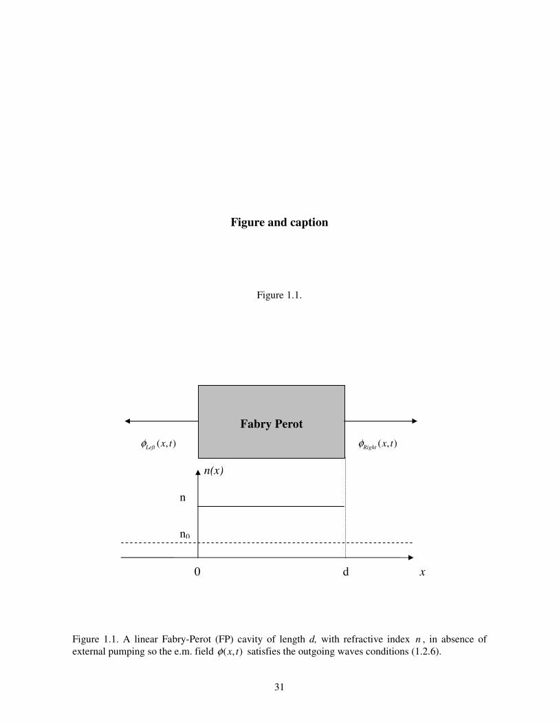
As schematically reported in fig. 1.1, consider a particular class of refractive index:
0
, [0, ]( )
, outsiden x d
n xn
∈=
. (1.4.1)
If the e.m. field equation (1.2.3) is solved, adding the outgoing waves conditions (1.2.7), the
QNM’s frequencies of the linear and homogeneous cavity are calculated, as shown in the following
relations:
k k iω α β= − , (1.4.2)
where
0
0
1 , ln , 0, 1, 2,...
( / ) ( / )n n
kn c d n c d n n
πα β += = ∈ = ± ± −
, (1.4.3)
being n just the refractive index of linear FP cavity. The QNM’s functions of the linear and
homogeneous cavity are calculated as:
00( ) cos sink k
k
nf x K n x i n x
c n cω ω = −
, (1.4.4)
where 0K is a suitable constant of normalization. The QNM’s functions (1.4.4) can be re-expressed
as in the following expression:
( )k kin x in x
c ckf x Ae Be
ω ω−
= + , (1.4.5)
being the coefficients A and B equal to: 0 0
2K n n
An−= and 0 0
2K n n
Bn+= .
Some useful results are reported, involving the QNM’s frequencies (1.4.2)-(1.4.3):

28
( ) ( )* *
2 20
2 2 2 20 0
0 0
0 0
22 20 0
0
2cos 1 , sin 1
( 1) , ( 1)
,
k k k k
k k
k kk k
nd nd nd ndi i i ik kc c c c
nd ndi i
c c
nd n n nd ni
c n n c n n
n n n ne e e e
n n n n
n n n ne e
n n n n
ω ω ω ω
ω ω
ω ω
− −
−
+ = − = − − − −
+ −= = − = = −− +
+ −= = − +
2
0
. (1.4.6)
Applying eqs. (1.4.6), in the case of a linear FP cavity, it is immediately demonstrable that: the
QNM’s frequencies (1.4.2) and the QNM’s functions (1.4.4) satisfy the general properties
[1]
*
*( ) ( )k k
k kf x f x
ω ω−
−
= −
=; (1.4.7)
besides, the outgoing wave conditions (1.2.7), referred to the QNMs, can be specified as shown in
the following relations:
0
( ) ( 1) (0)
( ) ( 1) ( )
kk k
kx k x kx d x
f d f
f x f x= =
= −∂ = − − ∂
. (1.4.8)
An useful integral is ,0
( ) ( ) ( )d
n m n mI x f x f x dxρ= which can be calculated as
2 2 2
2 0 0 0, 0 , 2
1 ( 1)( ) 2
n m
n m n mn m
n K n nI K d
c i cδ
ω ω
+ −+ −= ++
, (1.4.9)
where ,n mδ is the Kronecker’s delta. Eq. (1.4.9) is derived after some algebra, first inserting eqs.
(1.4.5) and then reminding eqs. (1.4.6).
The norm of the QNM’s function (1.4.4) is a complex number, given by the following expression
[1]:
2 2 20
0
2 ( ) ( ) [ (0) ( )]d
k k k k
nx f x dx i f f d
cω ρ= + +k kf f , (1.4.10)
being the main difference with the ordinary definition of norm the presence of 2 ( )kf x rather than
2( )kf x and the two additive “surfaces terms” 20( / ) (0)ki n c f and 2
0( / ) ( )ki n c f d .
Applying eq. (1.4.9), in the case of a linear and homogeneous cavity, it is immediately
demonstrable that: the QNM’s norm (1.4.10) for the linear and homogeneous cavity with the
QNM’s frequencies (1.4.2)-(1.4.3) and the QNM’s functions (1.4.5) assumes the form:
2 2
2 00 2 k
n nK d
cω−= ⋅k kf f . (1.4.11)

29
If a normalized version of the QNM’s function is adopted, corresponding to 2 kω=k kf f , then
the constant 0K is fixed, 2
20 2 2
0
2( )
cK
n n d=
−, so that:
0 02 20
2(0) , ( ) ( 1)
( )k
k kf K c f d Kn n d
= = = −−
. (1.4.12)
Besides, applying eq. (1.4.9), the orthogonality condition can be immediately derived for the
QNM’s functions
[1]:
0
0
2 2 20 00 0 0
( ) ( ) ( ) ( ) [ (0) (0) ( ) ( )]
1 ( 1)( ) [ ( 1) ] 0
( )
d
n m n m n m n m
n mn m
n mn m
nf x x f x dx i f f f d f d
c
n nK i K K n m
c i c
ω ω ρ
ω ωω ω
++
= + + + =
+ −= + + + − = ≠+
n mf f
, . (1.4.13)
5. Discussion and conclusions.
The e.m. field inside an open cavity can be obtained by suitable methods as the transfer
matrix [1] or the ray method [2]. The representation of the e.m. field inside an open cavity can be
given also as a superposition of Quasi Normal Modes (QNMs)
[1] which describe the coupling between the cavity and the environment. The importance of the
QNM’s approach lies in the fact that it is possible to recover the orthogonal representation of the
e.m. field, as it is necessary to consider quantum processes.
In general, an optical cavity is not a conservative system, so the natural evolution of the e.m. field
can not be described by an hermitian operator and the treatment of the e.m. field in terms of Normal
Modes (NMs) has to be dropped. The QNM’s approach considers the realistic situation in which the
open cavity is enclosed in an infinite external space. The lack of energy conservation for the open
cavity gives complex, instead of real, eigen frequencies. The evolution operator for the system is
not hermitian and the modes of the e.m. field are not normal but quasi-normal. In fact, under some
conditions over the refractive index: (a) the evolution of the QNMs is similar to the hermitian one
for the NMs, and (b) the e.m. field can be described as a superposition of QNMs only inside the
cavity and the QNM’s functions form an orthogonal basis only according to a non-canonical
metrics. The QNM’s functions do not represent the e.m. field outside of the cavity while they
represent the “not stationary” modes into the cavity. For the reason of not being complete in the
whole space, they are called “quasi-normal” modes. The QNM’s approach is very different from the
pseudo-mode one introduced by Dalton ed al. in ref. [3]. In fact, the pseudo-modes are obtained by
30
a Fano’s transformation of the NMs, they are defined as pseudo-modes because they depend on the
external pumping, and they use an ordinary metric; the QNMs are actual modes because they are
defined in absence of an external pumping, and they use a specific definition of complex metric.
In this chapter, some necessary results of ref. [6] have been stated; in ref. [6], the QNM’s approach
is discussed for double side open and inhomogeneous cavities. The description of the scalar field in
1D open cavities has been represented in terms of QNMs; the QNM’s description has been
extended from an one side open and homogeneous cavity
[1] to an open cavity from both ends, with an inhomogeneous distribution of refractive index.
References
[1] D.R. Hall and P.E. Jackson, The Physics and Technology of Laser Resonators (Adam Hilger,
Bristol, 1989); Y.A. Anan’ev, Laser Resonators and the Beam Divergence Problem (Adam Hilger,
Bristol, 1992).
[2] M. Born and E. Wolf, Principles of Optics (Macmillan, New York, 1964).
[3] A.W. Crook, J. Opt. Soc. Am. A 38, 954 (1948).
[4] D.N. Paltanayou and E. Wolf, Phys. Rev. D 13, 913 (1976); B.J. Hoenders, J. Math. Phys. 20,
329 (1979).
[5] Donald G. Dudley, Mathematical Foundations for Electromagnetic Theory (IEEE Press, New
York, 1994).
[6] F. DeMartini, G. Innocenti, G.R. Jacobovitz, and P. Mataloni, Phys. Rev. Lett. 59, 2955 (1987);
D.J. Heinzen, J.J. Childs, J.E. Thomas, and M.S. Feld, Phys. Rev. Lett. 58, 1320 (1987); A. E.
Siegmann, Phys. Rev. A 39, 1253 (1989).
[7] P. T. Leung, S. Y. Liu, and K. Young, Phys. Rev. A, 49, 3057 (1994); P. T. Leung, S. S. Tong,
and K. Young, J. Phys. A 30, 2139 (1997); P. T. Leung, S. S. Tong, and K. Young, J. Phys. A 30,
2153 (1997); E. S. C. Ching, P. T. Leung, A. Maassen van der Brink, W. M. Suen, S. S. Tong, and
K. Young, Rev. Mod. Phys., 70, 1545 (1998).
[8] C. Cohen-Tannoudji, B. Diu, F. Laloe, Quantum Mechanics (John Wiley, New York, 1977); W.
H. Louisell, Quantum Statistical Properties of Radiation (John Wiley, New York, 1973).
[9] A. Settimi, Studio del campo elettromagnetico alle frequenze ottiche nei cristalli fotonici uni-
dimensionali tramite la teoria dei quasi normal modes, Master Thesis (University of Rome “La
Sapienza”, Rome, 2002).
[10] P. T. Leung, W. M. Suen, C. P. Sun and K. Young, Phys. Rev. E, 57, 6101 (1998).
[11] R. Banerjee, P. Mukherjee, J. Phys. A 35, 5591 (2002).
[12] B. J. Dalton, Stephen M. Barnett, and B. M. Garraway, Phys. Rev. A. 64, 053813 (2001).
31
Figure and caption
Figure 1.1.
Figure 1.1. A linear Fabry-Perot (FP) cavity of length d, with refractive index n , in absence of external pumping so the e.m. field ( , )x tφ satisfies the outgoing waves conditions (1.2.6).
Fabry Perot
x
n(x)
0 d
n0
( , )Left x tφ ( , )Right x tφ
n

32
Chapter 2
QNM’s approach for open cavities
in absence of external pumping:
an application to one dimensional Photonic Crystals.
1. Introduction.
The past two decades have witnessed an intense investigation on electromagnetic
propagation phenomena at optical frequencies in periodic structures, usually referred to as one
dimensional (1D) Photonic Band Gap (PBG) structures [3]-[5]. These structures can be realized by
a stack of dielectric layers, arranged according to some periodic or quasi-periodic sequence. Usually
they are made alternating layers of high and low index materials of suitable thickness. If the 1D-
PBG structure is periodic it may be thought as done by the superposition of a finite number of equal
cells, each cell being usually constructed by two materials. The essential property of these 1D-PBG
structures is the existence of allowed and forbidden frequency bands and gaps, in analogy with the
energy bands and gaps in the semiconductors. At the same time, the distribution of the e.m. field
intensity along the structure strongly changes by changing the frequency or, in general if the e.m.
field is coming from outside, the boundary conditions. The 1D-PBG structures can be considered a
special case of an open cavity and have great importance in nonlinear processes [4]-[6].
The dispersive properties are usually evaluated assuming an infinite periodic structure [7]. The
finite dimensions of a 1D-PBG structure conceptually modify the calculation and the nature of the

33
dispersive properties: this is mainly due to the existence of an energy flow into and out of the
crystal. The application of the effective-medium approach to a 1D-PBG structure is discussed, and
the analogy of a 1D-PBG to a simple Fabry-Perot is developed by Sipe et al. in ref. [8]. A
phenomenological approach to the 1D-PBG’s dispersive properties has been presented in ref. [9].
In this chapter, the Quasi Normal Mode’s (QNM’s) approach
[1], even if limited to open cavities in absence of an external pumping, is applied to 1D-PBG
structures as open cavities from both sides [6]. The chapter is organized as follows. In section 2, the
QNM’s approach is deeper examined [7] so that the definition of the QNM’s eigen frequencies and
functions is better clarified respect to ref. [6]. In section 3, the completeness of the QNM’s
representation is proved inside 1D-PBG structures. In section 4, the equation for the QNM’s eigen
frequencies is derived for symmetric Quarter Wave (QW) 1D-PBGs. Conclusions are given in
section 5.
2. Examining deeper QNM’s approach.
In this section, the role of the complex Green’s function formalism is put into evidence for the
definition of the Quasi Normal Modes (QNMs); these considerations are here reported in more
details respect to ones already presented in ref [7]. With reference to figure 2.1, consider now an
open cavity of length d, filled with a refractive index ( )n x , which is enclosed in an infinite external
space. The cavity includes also the terminal surfaces, so it is represented as [0, ]C d= and the rest
of universe as ( ,0) ( , )U d= −∞ ∪ ∞ .
The e.m. field ( , )E x t in the cavity satisfies the equation [1]
2 2
2 2( ) ( , ) 0x E x tx t
ρ ∂ ∂− = ∂ ∂ , (2.2.1)
where 2( ) [ ( ) / ]x n x cρ = , and c is the speed of light in vacuum. If there is no external pumping, the
e.m. field satisfies suitable “outgoing waves conditions”
[1]
0
0
( , ) ( , ) for 0
( , ) ( , ) for
x t
x t
E x t E x t x
E x t E x t x d
ρ
ρ
∂ = ∂ <
∂ = − ∂ >
, (2.2.2)
where 20 0( / )n cρ = , and 0n is the outside refractive index. To take the cavity leakages into account,
the Laplace’s transform of the e.m. field is considered
0
( , ) ( , ) exp( )E x E x t i t dtω ω∞
= , (2.2.3)
34
where ω is a complex frequency. The e.m. field has to satisfy the Sommerfeld’s radiative
condition:
lim ( , ) 0x
E x ω→±∞
= . (2.2.4)
The Laplace’s transform of the e. m. field converges to an analytic function ( , )E x ω only over the
half-plane of convergence Im 0ω > . In fact, if the Laplace transform (2.2.3) is applied to the
“outgoing waves conditions” (2.2.2), it follows
0
0
( , ) ( , ) for 0
( , ) ( , ) for
x
x
E x i E x x
E x i E x x d
ω ω ρ ω
ω ω ρ ω
∂ = − <
∂ = >
, (2.2.5)
and solving the last equation of (2.2.5),
0 0 0( , ) exp( ) exp( Re )exp( Im ) for E x i x i x x x dω ω ρ ω ρ ω ρ∝ = − > . (2.2.6)
The Sommerfeld radiative condition (2.2.4) can be satisfied only if Im 0ω > .
The transformed Green’s function ( , , )G x x ω′ can be defined by [1]
2
22 ( ) ( , , ) ( )x G x x x x
xω ρ ω δ ∂ ′ ′+ = − − ∂
; (2.2.7)
it is an e.m. field so, over the half-plane of convergence Im 0ω > , it satisfies the Sommerfeld’s
radiative conditions
0
0
exp( ) 0 for ( , , )
exp( ) 0 for
i x xG x x
i x x
ω ρω
ω ρ
→ → ∞′ = − → → −∞
. (2.2.8)
Two “auxiliary functions” ( , )g x ω± can be defined by
2
22 ( ) ( , ) 0x g x
xω ρ ω±
∂ + = ∂ ; (2.2.9)
they are not defined as e.m. fields, because, over the half-plane of convergence Im 0ω > , they
satisfy only the “asymptotic conditions”
[1]:
0
0
( , ) exp( ) 0 for
( , ) exp( ) 0 for
g x i x x
g x i x x
ω ω ρ
ω ω ρ+
−
= → → ∞
= − → → −∞
. (2.2.10)
However, the transformed Green’s function ( , , )G x x ω′ can be calculated in terms of the “auxiliary
functions” ( , )g x ω± . In fact, it can be shown that
[1] the Wronskian associated to the two “auxiliary functions” ( , )g x ω± is x-independent
( ) ( , ) ( , ) ( , ) ( , )W g x g x g x g xω ω ω ω ω+ − − +′ ′= − , (2.2.11)

35
and for the transformed Green’s function:
( , ) ( , ) for
( )( , , )
( , ) ( , ) for
( )
g x g xx x
WG x x
g x g xx x
W
ω ωω
ωω ω
ω
− +
+ −
′ ′− <′ = ′ ′− <
. (2.2.12)
In what follows it is proved that, just for the “asymptotic conditions” (2.2.10), the “auxiliary
functions” ( , )g x ω± are linearly independent over the half-plane of convergence Im 0ω > , and so
the transformed Green function ( , , )G x x ω′ is analytic over Im 0ω > .
The “asymptotic conditions” establish that, only over the half-plane of convergence Im 0ω > , the
auxiliary function ( , )g x ω+ acts as an e.m. field for large x, because it is exponentially decaying; in
fact, from eq. (2.2.10): 0 0 0( , ) exp( ) exp( Re )exp( Im ) 0g x i x i x xω ω ρ ω ρ ω ρ+ = = − → for
x → ∞ . Then, still over the half-plane of convergence Im 0ω > , the other auxiliary function
( , )g x ω− in general does not act as an e.m. field for large x, so it is exponentially increasing; in fact,
according to eq. (2.2.10): 0 0( , ) ( ) exp( ) ( )exp( )g x A i x B i xω ω ω ρ ω ω ρ− = + − for x → ∞ , with
( ) 0B ω ≠ , and so 0 0 0( , ) ( ) exp( ) ( ) exp( Re )exp(Im )g x B i x B i x xω ω ω ρ ω ω ρ ω ρ− ≈ − = − → ∞ ,
for x → ∞ . It follows that the “auxiliary functions” ( , )g x ω± are linearly independent over the half-
plane of convergence Im 0ω > , because the Wronskian ( )W ω is not null; in fact, from eq. (2.2.11):
0( ) lim[ ( , ) ( , ) ( , ) ( , )] 2 ( ) 0x
W g x g x g x g x i Bω ω ω ω ω ρ ω ω+ − − +→∞′ ′= − = ≠ over Im 0ω > . So, the
transformed Green’s function ( , , )G x x ω′ is analytic over the half-plane of convergence Im 0ω > ,
where ( , , )G x x ω′ does not diverge; in fact, from eq. (2.2.12): ( , , ) 1/ ( )G x x Wω ω′ ∝ , with
( ) 0W ω ≠ over Im 0ω > .
The transformed Green’s function ( , , )G x x ω′ can be extended also over the lower complex
half-plane Im 0ω < , for analytic continuation [14]. According to [15], over the lower complex half-
plane Im 0ω < , it is always possible to define an infinite set of frequencies which are the poles of
the transformed Green’s function ( , , )G x x ω′ ; in other words, there exists an infinite set of complex
frequencies 0, 1, 2,nω ∈ = ± ± , with negative imaginary parts Im 0nω < , for which the
Wronskian (2.2.11) is null:
( ) 0nW ω = . (2.2.13)
The poles of the transformed Green’s function are referred as Quasi-Normal-Mode’s eigen
frequencies [15]. The definition of the QNM’s frequencies implies that the “auxiliary functions”

36
( , )g x ω± become linearly dependent when they are calculated in the QNM’s frequencies
0, 1, 2,nω ∈ = ± ± ; so, the auxiliary functions in the QNM’s frequencies are such that
( , ) ( ) ( , ) ( )n n n ng x c g x f xω ω ω+ −= = , (2.2.14)
where ( )nc ω is an suitable complex constant. The above functions ( )nf x are referred Quasi-
Normal-Mode eigen functions [15].
Applying the QNM’s condition (2.2.14) to the equation for the “auxiliary functions” (2.2.9), it
follows that the QNMs [ , ( )]n nf xω satisfy the equation:
2
22 ( ) ( ) 0n nx f x
xω ρ ∂ + = ∂
. (2.2.15)
Moreover, applying the QNM’s condition (2.2.14) to the “asymptotic conditions” for the “auxiliary
functions” (2.2.10), it follows that, outside the cavity, the QNMs do not represent e.m. fields
because they satisfy the QNM’s “asymptotic conditions”
0( ) exp( ) for n nf x i x xω ρ= ± → ∞ → ±∞ , (2.2.16)
while, into the cavity, the QNMs represent not stationary modes, so the QNM’s “outgoing waves
conditions” can be imposed at the terminal surfaces:
00
0
( ) (0)
( ) ( )
x n nx
x n nx d
f x i f
f x i f d
ω ρ
ω ρ=
=
∂ = −
∂ =
. (2.2.17)
Under the condition of QNM’s completeness
[1], the Green’s function is calculated as superposition of QNMs, only inside the cavity
( ) ( )
( , ; ) , for , [0, ]2
ni tn n
n n
F x F xiG x x t e x x d− ω′′ ′= ∈
ω , (2.2.18)
where are introduced the normalized QNM’s functions ( ) ( ) 2n n nF x f x= ω n nf f , denoting the
QNM’s norm as n nf f .
3. Completeness of QNM’s representation inside 1D-PC cavities.
In this section, the completeness of Quasi Normal Modes’s (QNM’s) representation is proved
inside one dimensional (1D) Photonic Crystal (PC) cavities (see ref. [6]). As depicted in figure
2.2.a, consider now a 1D-PC as a cavity open at both ends, with refractive index which is
continuous in some intervals:

37
0 0
1
1
( ) , for
( ) ( ) , for , where [1, ]
( ) , for k k k
N N
n x x x
n x n x x x x k N
n x x x−
+
<= < < ∈ >
. (2.3.1)
Outside the 1D-PC cavity there is a medium with an asymptotic refractive index:
0 1 0lim ( ) lim ( )Nx xn x n x n+→−∞ →∞
= = . (2.3.2)
The QNM’s representation is complete only inside the 1D-PC cavity. In what follows it is proved
that, inside a 1D-PC cavity, the condition of QNM’s completeness is valid, i.e. the behaviour of
( , , )G x x ω′ for large ω is (see ref.
[1] for details):
lim ( , , ) 0, Im( ) 0G x xω
ω ω ω→∞
′ = ∀ < . (2.3.3)
The proof of QNM’s completeness is based on the application of the WKB method extended to
optical regime. The WKB method was proposed to solve the Schrödinger’s equation (so applied to
the Planck’s constant , considering 0→ ) and here is proposed in Optics (but applied to the e.m.
field wavelength λ, considering λ→0) [6]. With reference to the 1D-PBG of refractive index (2.3.1)
, as depicted in figure 2.1.a, the equation (2.2.9) can not be solved exactly adding the asymptotic
conditions (2.2.10); however, a WKB-like method can be used in every period of the 1D-PC cavity,
if the wavelength λ is supposed so small to verify:
1
( ) 4, for , where [1, ]k
k k
dn xx x x k N
dxπλ −<< < < ∈ . (2.3.4)
For a 1D-PC cavity, whose refractive index is given by eq. (2.3.1), the following expressions are
obtained for the auxiliary function ( , )g x ω− (see ref. [6] for details)
0
( ) ( )
1
( )
0
( , ) ( ) ( ) ,
( , ) ,
x xk k
x x
x
x
i n d i n dc c
k k k k
i n dc
g x A e B e x x x
g x e x x
ω ωξ ξ ξ ξ
ω ξ ξ
ω ω ω
ω
−
− −
−
−
= + < <
= <
. (2.3.5)
where [1, 1]k N∈ + and +∞=+1Nx . For the auxiliary function ),( ωxg+ the following expressions
are obtained
1 1
( ) ( )
1
( )
( , ) ( ) ( ) ,
( , ) ,
x x
x xk k
x
xN
i n d i n dc c
k k k k
i n dc
N
g x C e D e x x x
g x e x x
ω ωξ ξ ξ ξ
ω ξ ξ
ω ω ω
ω
− −
−
+ −
+
= + < < = >
. (2.3.6)

38
where [0, ]k N∈ and −∞=−1x . Under the conditions of continuity for the auxiliary functions
( , )g x± ω and their derivatives in the points kx x= , it results
1
1
, [0, ]k k
k k
i ik k k k
k i ik k k k
A A e R B eS k N
B R A e B e
ϑ ϑ
ϑ ϑ
− −+
+
+ = ∈ +
. (2.3.7)
1 1
1 1
1 1
1 1
, [0, ]k k
k k
i ik k k k
k i ik k k k
C C e R D eS k N
D R C e D e
ϑ ϑ
ϑ ϑ
− −
− −
− −+ +
+ +
− ′= ∈ − + , (2.3.8)
where
1
( )
[ ( ) ( )][ ( ) ( )]
, [0, ][ ( ) ( )]
2 ( )
[ ( ) ( )]2 ( )
k
k
x
kx
k kk
k k
k kk
k
k kk
k
n x dxc
n x n xR
n x n xk N
n x n xS
n x
n x n xS
n x
ωϑ−
+ −
+ −
+ −
+
+ −
−
=
− = + ∈
+ = +′ =
. (2.3.9)
Now, only inside the 1D-PC cavity, i.e. 0( , ) | Nx x x x x x′ ′∀ < ≤ < , there exists a suitable value of k,
such that 0 1, k k Nx x x x x x−′< ≤ ≤ < , so it can be found a couple ( , )n m , such that 1 n k≤ ≤ and
k m N≤ ≤ , and it results:
( ) ( )
( , ) ( ) ( )
x xn n
x x
i n d i n dc c
n ng x A e B eω ωξ ξ ξ ξ
ω ω ω′ ′
−
−
′ = + , (2.3.10)
1 1
( ) ( )
( , ) ( ) ( )
x x
x xm m
i n d i n dc c
m mg x C e D e
ω ωξ ξ ξ ξ
ω ω ω− −
−
+
= + . (2.3.11)
Then, the Fourier’s transform of the Green’s function ( , , )G x x ω′ for x x′ ≤ has the following
expression [see eq. (2.2.12)]:
1 1
1 1
( ) ( )( ) ( )
( ) ( )
( ) ( ) ( ) ( )
( , , )
2 ( ) ( ) ( ) ( ) ( )
x xx xn n
x xx x m m
x xn n
x xm m
i n d i n di n d i n d c cc c
n n m m
i n d i n dc c
m n m n
A e B e C e D e
G x x
i n x D B e C A ec
ω ωω ω ξ ξ ξ ξξ ξ ξ ξ
ω ωξ ξ ξ ξ
ω ω ω ω
ωω ω ω ω ω
′ ′ − −
− −
−−
−
+ + ′ = −
−
. (2.3.12)
The coefficients , , , n n m mA B C D are obtained from eqs. (2.3.7) and (2.3.8) after some algebra:
2
10
1
0
1 1
0 0
n
k nk
n
kk
in n
kn nk
ik kn k
AA R eS
B Be
ϑ ϑ
ϑ
−−
=
−
=
−− −
= =
= ≅
∏ ∏ , (2.3.13)
39
1
1
1
11 1
N
k mk m
N
kk m
iN N
km N mk
ik m k mm kN
CC R R eS
D DR e
ϑ ϑ
ϑ
−−
=
−
= −
−
= + = +
′= ≅
−
∏ ∏ . (2.3.14)
If the refractive index is supposed such that ( ) ( ) 1, [0, ]k kn x n x n k N+ −− ≤ ∆ ≤ ∀ ∈ , then
[ ( ) ( )] 1 [ ( ) ( )] 1 2, [0, ]k k k k kR n n x n x n x n x k N+ − + −≤ ∆ + ≤ + < ∀ ∈ . If , [0, ],kR k N∀ ∈ is close to 0
than to 1, then, from eq. (2.3.13) and eq. (2.3.14), it follows that nB is dominant with respect to nA ,
and mD is dominant with respect to mC , so eq. (2.3.12) becomes:
1
1
( ) ( )
( )
( , , )
2 ( )
x xn
x xm
xn
xm
i n d n dc
i n dc
eG x x
i n x ec
ω ξ ξ ξ ξ
ω ξ ξω
ω
′ −
−
− +
−
′ ≅ −
. (2.3.15)
Since for x x′ ≤ , it follows
1 1 1
( ) ( ) ( ) ( ) ( )n n n
m m m
x x xx x
x x x x x
n d n d n d n d n dξ ξ ξ ξ ξ ξ ξ ξ ξ ξ− − −′ ′
+ = + ≤ . (2.3.16)
and the transformed Green’s function in a 1D-PC cavity has the following behaviour:
( , , ) 0 for G x x ω ω′ → → ∞ . (2.3.17)
Therefore, the QNM’s completeness in 1D-PC cavities is proved.
4. QNM’s frequencies for 1D-PBG structures.
The previous considerations can be specified for a symmetric 1D-PBG structure, consisting
on N periods plus one layer; every period is composed of two layers respectively with lengths h and
l and with refractive indices hn and ln , while the added layer is with parameters h and hn . With
reference to fig. 2.2.b, consider now a symmetric 1D-PBG structure, consisting of 2 1N + layers
with a total length ( )d N h l h= + + ; if the two layers external to the symmetric 1D-PBG structure
are counted, the 1D-space x can be divided into 2 3N + layers: they are
1[ , ] , 0,1, , 2 1,2 2k k kL x x k N N−= = + + , with 1 0 2 1 2 2, 0, , N Nx x x d x− + += −∞ = = = +∞ . The
refractive index ( )n x takes a constant value kn in every layer , 0,1, , 2 1, 2 2kL k N N= + + , i.e.
0 2 21 for ,
( ) for , 1,3, , 2 1, 2 1
for , 2, 4, , 2
N
h k
l k
x L L
n x n x L k N N
n x L k N
+∈= ∈ = … − + ∈ = …
. (2.4.1)

40
In Appendix A, it is proved that, introducing the two phase-terms
==
==
chnhq
clnlq
hhh
lll
ωδ
ωδ, (2.4.2)
the QNM’s frequencies can be found by solving the following transcendental equation
N-1 N-2k k2 2
N-1-2k N-2-2k
k 0 k 0
(-1) (N -1- k)! (-1) (N - 2 - k)!( ) ( ) 0
k! (N -1- 2k)! k! (N - 2 - 2k)!
= =
α γ + β γ = , (2.4.3)
where the coefficients γβα ,, are parameters related to the refractive indices of each layer:
h l
h l
22i ih l h l
l h 2l h l h l h
2-2i ih l h l
l h 2l h l h l h
2h l
l 2l l h
n n n n1 1 1n 2 n - 4 - 2 e
4 n n n n n n
n n n n1 1n - 2 n - 4 2 e
n n n n n n
n n12 n - 2
n n n
δ + δ
δ + δ
α = + + + + + +
+ + + + + + +
+ + +
l
h l
h l
i
22i -ih l h l
l h 2l h l h l h
2-2i -ih l h l
l h 2l h l h l h
2h l
l 2l l h
e
n n n n1 1- n 2 n - 4 2 - e
n n n n n n
n n n n1 1- n - 2 n - 4 - 2 - e
n n n n n n
n n1-2 n 2
n n n
δ
δ δ
δ δ
+ + + + + + +
+ + + + +
+ + + +
( ) ( ) ( ) ( ) ( ) ( ) ( ) ( )
l
h h
h l h l l h h l
-i
i -ih h
h h
2 2 2 2i i - i - -ih l h l h l h l
h l
e
1 12 - n e 2 n e
n n
1n n e n n e n n e n n e
4n n
δ
δ δ
δ +δ δ δ δ δ δ +δ
β = + + + + γ = + − − − − + +
.(2.4.4)
More details are given in Appendix A. For a symmetric quarter wave (QW) 1D-PBG with N periods
and refω as reference frequency, there are 2 1N + families of QNMs, i.e. , [0,2 ]QNMnG n N∈ ; the
QNMnG family of QNMs consists on infinite QNM’s frequencies, i.e. , , 0, 1, 2,n m mω ∈ = ± ± ,
which have the same imaginary part, i.e. , ,0Im Im , n m n mω ω= ∈ , and are aligned by a step
2 refω∆ = , i.e. , ,0Re Re , n m n m mω ω= + ∆ ∈ . It follows that, if the complex plane is divided into
some ranges, i.e. Re ( 1) , mR m m mω= ∆ ≤ < + ∆ ∈ , each of the QNM’s family QNMnG drops only
one QNM’s frequency over the range mR , i.e. , ,0 ,0(Re , Im )n m n nmω ω ω= + ∆ ; so, there are 2 1N +

41
QNM’s frequencies over the range mR and they can be referred as , ,0 , [0, 2 ]n m n m n Nω ω= + ∆ ∈ . It
results that there are 2 1N + QNM’s frequencies over the basic range, i.e. 0 0 ReS ω= ≤ < ∆ , and
they correspond to ,0 , [0, 2 ]n n Nω ∈ .
The QNM’s frequencies are not uniformly distributed in the complex plane, but they arrange
themselves in order to form permitted and forbidden bands, in agreement with the known
characteristics of the QW 1D-PBG structures [16]. In figure 2.3.a, the QNM’s frequencies are
plotted for a symmetric QW 1D-PBG, where the reference wavelength is 1ref mλ µ= , the number of
periods is N=4 and the two used refractive indices are nh=1.5, nl=1. Simple inspection of figure
2.3.a. shows that next to the gap, the QNM’s frequencies have the smallest imaginary part in
modulus, and hence have the narrowest resonance lines. In figure 2.3.b, the QNM’s frequencies are
shown for the same cavity of fig.2.3.a, but with nh=2, nl=1. Contrasting figs. 2.3.a. and 2.3.b, it can
be seen that as the difference between the refractive indices of adjacent layers is increased, the
width of the gap increases. This also entails that the magnitude of the imaginary part of the QNM’s
frequency decreases in modulus, and the resonance peaks become tighter. In figure 2.3.c, the
QNM’s frequencies are shown for the same cavity as above, with an increased number of periods
N=8 and nh=2, nl=1. Contrasting figs. 2.3.b. and 2.3.c, it can be seen that as the number of periods
is increased, the position of the gap remains the same: as in the previous case, the imaginary parts of
the QNM’s frequencies decrease in modulus, and the resonance peaks become narrower.
5. Conclusions.
One-dimensional (1D) Photonic Band Gap (PBG) structures are particular optical cavities,
with both sides open to the external environment and a stratified material inside. A 1D-PBG
structure is finite in space and, working with e.m. pulses of a spatial extension longer than the
length of the 1D-PBG, the open cavity cannot be studied as infinite: rather, the boundary conditions
must be considered at the two ends of the cavity.
In this chapter, the Quasi Normal Mode’s (QNM’s) approach, even if limited to open cavities in
absence of an external pumping, has been applied to 1D-PBG structures as open cavities from both
sides. The QNM’s approach has been deeper examined, so that the definition of the QNM’s
frequencies and functions has been better clarified. The completeness of the QNM’s representation
has been proved inside 1D-PBG structures. The equation for the QNM’s frequencies has been
derived for symmetric Quarter Wave (QW) 1D-PBGs. The QNM’s frequencies are not uniformly
distributed in the complex plane, but they arrange themselves in order to form permitted and
42
forbidden bands, in agreement with the known characteristics of the QW 1D-PBG; it has been
proved that, for a symmetric QW1D-PBG, with N periods and refω as reference frequency, there are
exactly 2N+1 QNM’s frequencies in the [0,2 )refω range.
Appendix A.
This appendix describes how to obtain the equation of the Quasi Normal Mode’s (QNM’s)
frequencies (2.4.3)-(2.4.4) for the symmetric one dimensional (1D) Photonic Band Gap (PBG)
structure of fig. 2.2.b. with refractive index (2.4.1). Then, this equation is solved for a quarter-wave
(QW) 1D-PBG.
The matrix method [17] is used for describing the 1D-PBG structures. The transmission matrix for a
single period of the 1D-PBG cavity has the form
11 12
21 22
Mµ µµ µ
=
, (2.A.1)
where
−=
−−=
+=
−=
lhh
llh
hlllhh
hll
lhh
lhl
hlh
δδδδµ
δδδδµ
δδδδµ
δδδδµ
sinsincoscos
cossincossin
cossin1
cossin1
sinsincoscos
22
21
12
11
. (2.A.2)
In the expression (2.A.2), the propagation constants in the two layers of a period ( )h hq n cω= ,
( )l lq n cω= and the respective phases h hq hδ = , l lq lδ = appear.
The transmission matrix of a symmetric 1D-PBG structure has the form
11 12
21 22PBG
m mM
m m
=
, (2.A.3)
where
11 11 1 2 21 1
12 12 1 22 1 2
21 11 1 2 21 1
22 12 1 22 1 2
sincos [ ( ) ( )] ( )
sincos ( ) [ ( ) ( )]
sin [ ( ) ( )] cos ( )
sin ( ) cos [ ( )]
hh N N N
h
hh N N N
h
h h N N h N
h h N h N N
m U U Uq
m U U Uq
m q U U U
m q U U U
δδ µ ϑ ϑ µ ϑ
δδ µ ϑ µ ϑ ϑ
δ µ ϑ ϑ δ µ ϑδ µ ϑ δ µ ϑ
− − −
− − −
− − −
− − −
= − + = + − = − − +
= − + −
. (2.A.4)

43
In expression (A.4.) the Chebyshev’s polynomials ϑ
ϑϑsinNsin
U N
])1[()(
+= with
argument2
cos 2211 µµϑ += appear.
As depicted in fig. 2.2.b, if )(xf is the wave function of a generic QNM and ( )f x′ is its spatial
derivative, then 0 0( , )f f ′ and 2 1 2 1( , )N Nf f+ +′ are their values at the input and output of a 1D-PBG
structure, such that:
2 1 0
2 1 0
NPBG
N
f fM
f f+
+
= ′ ′
. (2.A.5)
Referring to fig. 2.2.b, if the equation 2 2( ) ( ) 0x x f xρ ω ∂ + = of the e.m. field is solved in every
layer, the expression for the wave function of a generic QNM is obtained for a symmetric 1D-PBG
structure:
0 0
2 1 2 10
1
2 2 2 20
2 2 2 2
( ) ( )
[ ( )] [ ( ) ]
[ ( ) ] [( 1)( ) ]
h h
l l
i x i xc c
N i n x i n xc c
k kk
N i n x i n xc c
k kk
i x i xc c
N N
f x A e B e x
A e B e x k h l k h l h x
A e B e x k h l h k h l x
A e B e
ω ω
ω ω
ω ω
ω ω
ϑ
ϑ ϑ
ϑ ϑ
−
−
+ +=
− −
+ +=
−
+ +
= + − +
+ + − + + + − +
+ + − + − + + − +
+ +
[ ( ) ]x N h l hϑ
− + −
, (2.A.6)
where )(xϑ is the unitary step function. By imposing the conditions for QNM’s frequencies,
)exp()( cxixf ω±= to ±∞→x , it results 0)(0 =ωA and
( )[ ( ) ]2 1 2 12 2
( ) ( ) ( )( ) 0
2 ( )i c N h l hN N
N
i c f fB e
i cωω ω ωω
ω+ ++ +
+
′−= = . (2.A.7)
Eqs. (2.4.3) and (2.4.4) are obtained after some algebra from eq. (2.A.7), by inserting eq. (2.A.5),
(2.A.4) and (2.A.2).
Now, working with a QW 1D-PBG structure, it results
4ref
l hn l n hλ
= = , (2.A.8)
where refλ is a reference wavelength. With these assumptions, the phases lh δδ , become
l hδ δ δ= = , (2.A.9)
where the phase ( 4)( )ref cδ λ ω= is introduced. Equation (2.4.3) becomes a real coefficient
polynomial equation (instead of a transcendental equation) of degree 2 1N + in the variable ie δ .

44
There are 2 1N + families of QNMs and, if a generic one is picked, all the QNM’s frequencies have
the same imaginary part and are distributed with a step 2 ref∆ = ω , where 2ref refcω π λ= . Then,
there are exactly 2 1N + QNM’s frequencies in the [0,2 )refω range. From eq. (2.A.6), the QNM’s
functions )(xfn corresponding to the QNM’s frequencies nωω = can be constructed. By imposing
the conditions of continuity for the wave function )(xf and its spatial derivative )()( xfxg ′= at
interfaces of the symmetric QW 1D-PBG cavity, it results
h 0 h 0
0 0
h 0 h 0 0 0
h 0 h 0
h 0 h
in x in xc c
i x i xc c
h 01
in x in x i x i x 01 c c c c
h
in (x k(h l)) in (x k(h l))c c
h2k 1
in (x k(h l)) in2k 1 c c
h
1e e
n AA e e1BB 2 1
e e e en
1e e
nA 1B 2 1
e en
ω ω− −ω ω−
ω ω ω ω−
ω ω− + + − + +
+ω ω+ ++
= − −
=
−
l 0 l 0
l 0 l 00
l 0 l 0
l 0
in (x k(h l)) in (x k(h l))c c
2k
in (x k(h l)) in (x k(h l))(x k(h l)) 2kc cl l
in (x k(h l) h) in (x k(h l) h)c c
l2k 2
in (x k(h l)2k 2 c
e e AB
n e n e
1e e
nA 1B 2
e
ω ω+ + − + +
ω ω+ + − + ++ +
ω ω− + + + − + + +
+ω + ++
−
=
h 0 h 0
h 0 h 0l 0
0 0
in (x k(h l) h ) in (x k(h l) h )c c
2k 1
in (x k(h l) h) in (x k(h l) h )h ) in (x k(h l) h) 2k 1c cch h
l
i (x N(h l) h ) i (x N(h lc c
2N 2
2N 2
e e AB1
n e n een
A e e1B 2
ω ω+ + + − + + +
+ω ωω + + + − + + ++ + + + +
ω ω− + + + − + +
+
+
−−
=
h 0 h 0
h 0 h 00 0
in (x N(h l) h ) in (x N(h l) h)) h)c c
2N 1
in (x N(h l) h ) in (x N(h l) h)i (x N(h l) h ) i (x N(h l) h) 2N 1c cc ch h
Ae eB
n e n ee e
ω ω+ + + − + + ++
+ω ωω ω + + + − + + ++ + + + + + +
−− ,
(2.A.10)
where 0)(0 =nA ω and 2 2 ( ) 0N nB ω+ = .
References.
[1] S. John, Phys. Rev. Lett. 53, 2169 (1984); S. John, Phys. Rev. Lett. 58, 2486 (1987); E.
Yablonovitch, Phys. Rev. Lett. 58, 2059 (1987); E. Yablonovitch and T. J. Gmitter, Phys. Rev.
Lett.. 63, 1950 (1989).
[2] J. Maddox, Nature (London) 348, 481 (1990); E. Yablonovitch and K.M. Lenny, Nature
(London) 351, 278, 1991; J. D. Joannopoulos, P. R. Villeneuve, and S. H. Fan, Nature (London)
386, 143 (1997).
[3] J. D. Joannopoulos, Photonic Crystals: Molding the Flow of Light (Princeton University Press,
Princeton, New York, 1995); K. Sakoda, Optical properties of photonic crystals (Springer Verlag,
Berlin, 2001); K. Inoue and K. Ohtaka, Photonic Crystals: Physics, Fabrication, and Applications
(Springer-Verlag, Berlin, 2004).
45
[4] J. P. Dowling and C. M. Bowden, Phys. Rev. A 46, 612 (1992); M. J. Bloemer and M. Scalora,
Appl. Phys. Lett. 72, 1676 (1998); I. S. Fogel, J. M. Bendickson, M. D. Tocci, M. J. Bloemer, M.
Scalora, C. M. Bowden, and J. P. Dowling, Pure Appl. Opt. 7, 393 (1998); C. M. Bowden and A.
Zheltikov, J. Opt. Soc. Am. B 19, 2046 (2002).
[5] M. Centini, C. Sibilia, M. Scalora, G. D’Aguanno, M. Bertolotti, M. J. Bloemer, C. M. Bowden,
and I. Nefedov, Phys.Rev E 60, 4891 (1999); Y. Dumeige, P. Vidakovic, S. Sauvage, I. Sagnes, J.
A. Levenson, C. Sibilia, M. Centini, G. D’Aguanno, and M. Scalora, Appl. Phys. Lett. 78, 3021 (
2001); M. Scalora, M. J. Bloemer, C. M. Bowden, G. D’Aguanno, M. Centini, C. Sibilia, M.
Bertolotti, Y. Dumeige, I. Sagnes, P. Vidakovic, and A. Levenson, Opt. Photonics News 12, 36
(2001).
[6] Nanoscale Linear and Nonlinear Optics, edited by M. Bertolotti, C. M. Bowden, and C. Sibilia,
AIP Conf. Proc. No. 560 (AIP, Melville, New York, 2001).
[7] P. Yeh, Optical Waves in Layered Media (Wiley, New York, 1988).
[8] J. E. Sipe, L. Poladian, C. Martijn de Sterke, J. Opt. Soc. Am. A 11, 1307 (1994).
[9] G. D’Aguanno, M. Centini, M. Scalora, C. Sibilia, M.J. Bloemer, C.M. Bowden, J.W. Haus, M.
Bertolotti, Phys. Rev. E 63, 036610 (2001).
[10] P. T. Leung, S. Y. Liu, and K. Young, Phys. Rev. A, 49, 3057 (1994); P. T. Leung, S. S. Tong,
and K. Young, J. Phys. A 30, 2139 (1997); P. T. Leung, S. S. Tong, and K. Young, J. Phys. A 30,
2153 (1997); E. S. C. Ching, P. T. Leung, A. Maassen van der Brink, W. M. Suen, S. S. Tong, and
K. Young, Rev. Mod. Phys. 70, 1545 (1998); P. T. Leung, W. M. Suen, C. P. Sun and K. Young,
Phys. Rev. E, 57, 6101 (1998).
[11] A. Settimi, S. Severini, N. Mattiucci, C. Sibilia, M. Centini, G. D’Aguanno, M. Bertolotti, M.
Scalora, M. Bloemer, C. M. Bowden, Phys. Rev. E, 68, 026614 (2003).
[12] S. Severini, A. Settimi, C. Sibilia, M. Bertolotti, A. Napoli, A. Messina, Quasi Normal
Frequencies in open cavities: an application to Photonic Crystals, in press on Acta Phys. Hung. B
(2006).
[13] M. Born and E. Wolf, Principles of Optics (Macmillan, New York, 1964).
[14] G. F. Carrier, M. Krook, C. E. Pearson, Functions of a complex variable – theory and
technique (McGraw-Hill Book Company, New York, 1983).
[15] A. Bachelot, A. Motet-Bachelot, Ann. Inst. Henry Poincare 59, 3, (1993).
[16] D. W. L. Sprung, H. Wu, and J. Martorell, Am. J. Phys. 61, 1118 (1993); M. G. Rozman, P.
Reineken, and R. Tehver, Phys. Lett. A 187, 127 (1994).
[17] J. Lekner, Theory of Reflection (Martinus Nijhoff, Dordrecht, 1987).

46
Figures and captions
Figure 2.1.
Open Cavity
x
n(x)
0 d
1
ELeft(x,t) ERight(x,t)
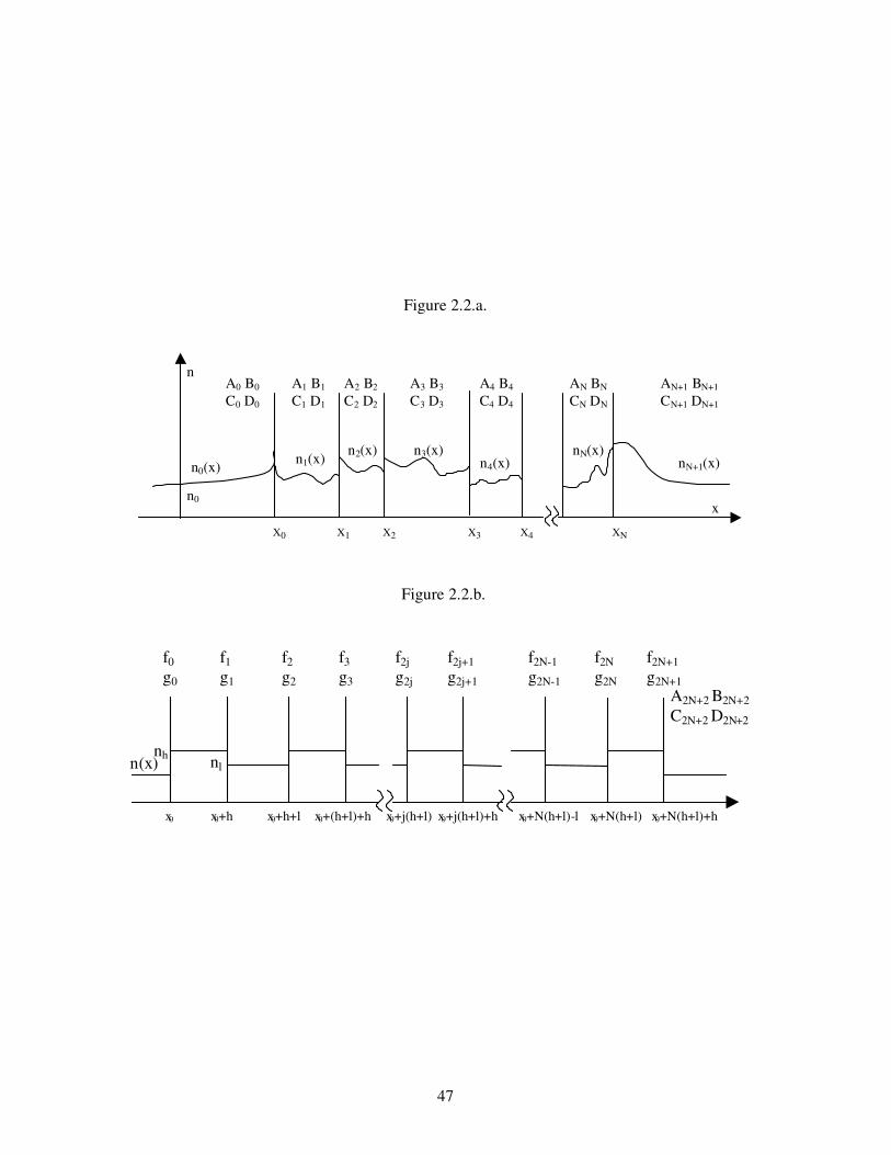
47
Figure 2.2.a.
Figure 2.2.b.
x 0
A 2N+2 B 2N+2 C 2N+2 D 2N +2
n(x) n h n l
x 0 +h x 0 +h+l x 0 +( h+l)+h x 0 +j( h+l)+h x 0 +j( h+l) x 0 +N( h+l)-l x 0 +N( h+l)+h x 0 +N( h+l)
f 0 g 0
f 1 g 1
f 2 g 2
f 3 g 3
f 2j g 2j
f 2N+1 g 2N+1
f 2N g 2N
f 2j+1 g 2j+1
f 2N-1 g 2N-1
X 0 X 1 X 2 X 3 X 4 X N
A 1 B 1 C 1 D 1
A 0 B 0 C 0 D 0
A 2 B 2 C 2 D 2
A 3 B 3 C 3 D 3
A 4 B 4 C 4 D 4
A N B N C N D N
A N+1 B N+1 C N+1 D N+1
n 0
n 0 (x)
n
x
n 1 (x) n 2 (x) n 3 (x) n 4 (x)
n N (x) n N+1 (x)
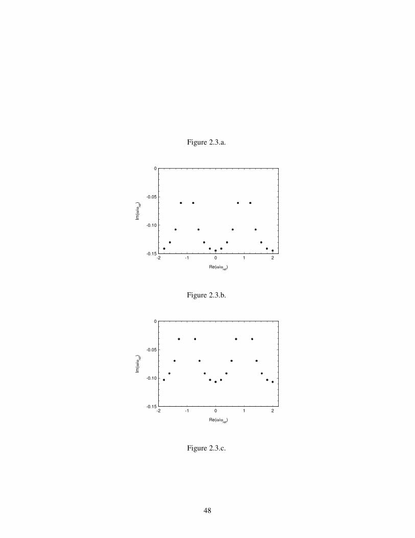
48
Figure 2.3.a.
Figure 2.3.b.
Figure 2.3.c.
-0.15
-0.10
-0.05
0
-2 -1 0 1 2
Re(ω/ωref
)
Im(ω
/ωre
f)
-0.15
-0.10
-0.05
0
-2 -1 0 1 2
Re(ω/ωref
)
Im(ω
/ωre
f)
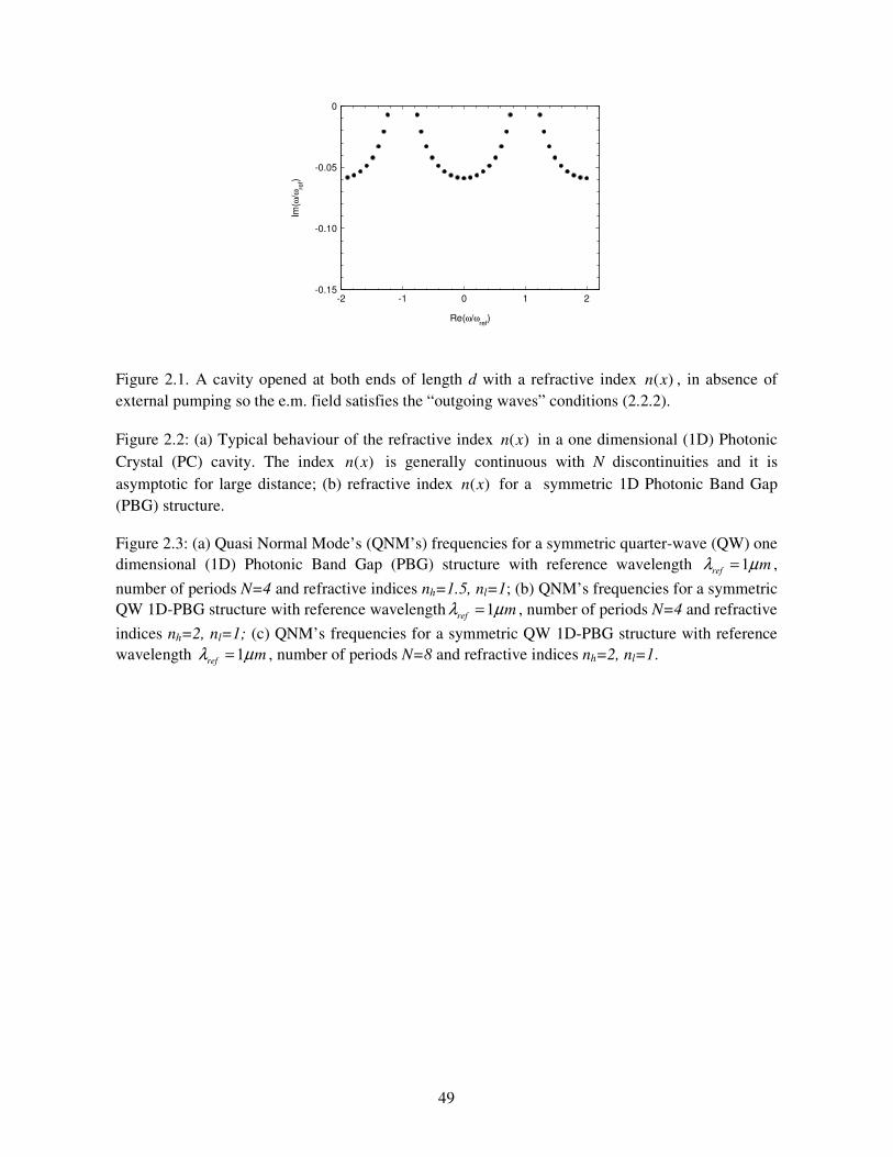
49
Figure 2.1. A cavity opened at both ends of length d with a refractive index ( )n x , in absence of external pumping so the e.m. field satisfies the “outgoing waves” conditions (2.2.2). Figure 2.2: (a) Typical behaviour of the refractive index ( )n x in a one dimensional (1D) Photonic Crystal (PC) cavity. The index ( )n x is generally continuous with N discontinuities and it is asymptotic for large distance; (b) refractive index ( )n x for a symmetric 1D Photonic Band Gap (PBG) structure. Figure 2.3: (a) Quasi Normal Mode’s (QNM’s) frequencies for a symmetric quarter-wave (QW) one dimensional (1D) Photonic Band Gap (PBG) structure with reference wavelength 1ref mλ µ= , number of periods N=4 and refractive indices nh=1.5, nl=1; (b) QNM’s frequencies for a symmetric QW 1D-PBG structure with reference wavelength 1ref mλ µ= , number of periods N=4 and refractive indices nh=2, nl=1; (c) QNM’s frequencies for a symmetric QW 1D-PBG structure with reference wavelength 1ref mλ µ= , number of periods N=8 and refractive indices nh=2, nl=1.
-0.15
-0.10
-0.05
0
-2 -1 0 1 2
Re(ω/ωref
)
Im(ω
/ωre
f)

50
Chapter 3
QNM’s approach for open cavities
excited by an external pumping:
Transmission properties of a 1D-PBG structure.
1. Introduction.
The definition of natural modes for confined structures is one of the central problems in
physics [4], as in nuclear physics, astrophysics, etc. The main problem is due to the boundary
conditions, when they are such to push out the problem from the class of Sturm-Liouville. This
occurs when boundary conditions imply the presence of eigen-values, as for example when a
scatterer excited from the outside [5] gives rise to a transmitted and reflected field. An open cavity
with an external or internal excitation represents a “non-canonical “ problem, in the sense of a
Sturm–Liouville’s problem, due to the fact that the cavity modes couple themselves with the
external modes.
One dimensional (1D) Photonic Band Gap (PBG) structures [3]-[5] of finite length manifest all the
aspects related to a class of problems which do not belong to the Sturm-Liouville’s class: in fact,
they behave as scattering objects when they are excited from outside and as open cavities when
excited from the inside.
51
In this chapter, the Quasi Normal Mode’s (QNM’s) approach, defined for an open cavity in absence
of an external pumping
[1], is extended to the e.m. problem of a cavity which is excited by an external pump [7]; then, the
QNM’s approach is applied to a symmetric quarter wave (QW) 1D-PBG structure to discuss its
transmission properties [6]. The chapter is organized as follows. In section 2, the transmission
coefficient for an open cavity is calculated as a QNM’s super-position. In section 3, a transmission
coefficient formula is obtained for a symmetric QW 1D-PBG structure. Moreover, the transmission
properties are discussed in terms of the QNM’s eigen frequencies. Then, the “e.m. modes”, i.e. the
field distributions at the transmission resonances, are obtained as super-positions of the QNM’s
eigen functions. Finally, the external pumping of the 1D-PBG structure is generalized as two
counter-propagating field pumps, showing the e.m. interference inside the cavity of the two field
pumps. Conclusions are given in section 4.
2. Extending QNM’s approach:
e.m. problem of an open cavity excited by an external pump.
In this section, the Quasi Normal Mode’s (QNM’s) approach is extended to the e.m. problem
of an open cavity which is excited by an external pump; these considerations are here reported in
more details respect to ones already presented in ref [7]. With reference to fig. 3.1., consider now an
open cavity of length d, with a refractive index ( )n x and excited by a pump ( ) ( , )PE x t incoming
from the left side.
Under these conditions, the QNM’s functions form a complete basis only inside the open cavity,
and the e.m. field can be calculated as a superposition of QNMs [2]
( , ) ( ) ( ), for 0n nn
E x t a t F x x d= ≤ ≤ , (3.2.1)
where are introduced the normalized QNM’s functions ( ) ( ) 2 /n n nF x f x ω= n nf f , denoting the
QNM’s norm as n nf f . The superposition coefficients satisfy the dynamic equation [2]
0
( ) ( ) (0) ( )2
n n n n
n
ia t i a t F J tω
ω ρ+ = , (3.2.2)
where is defined a driving force: ( )0 0
( ) 2 ( , )Px x
J t E x tρ=
= − ∂ . The left-pump satisfies the
“incoming wave condition” [2]:
( ) ( )0 00
( ) 2 ( , ) 2 (0, )P Px tx
J t E x t E tρ ρ=
= − ∂ = ∂ . (3.2.3)

52
Each QNM is driven by the driving force ( )J t and decays at the same time because of Im 0nω < .
The coupling to the force is determined by the surface value (0)nF of the QNM’s function. The
open cavity is in a steady state, so the Fourier’s transform with a real frequency
( , ) ( , ) exp( )E x E x t i t dtω ω∞
−∞
= can be applied to equations (3.2.1)-(3.2.3), and it follows
0
( )0
( , ) ( ) ( )
(0) ( )( )
2
( ) 2 (0, )
n nn
nn
nn
P
E x a F x
F Ja
J i E
ω ω
ωωω ωω ρ
ω ρ ω ω
= = − = −
, (3.2.4)
so
0
(0) ( )( , ) (0, )
( )n n
Pn n n
F F xE x E iω ω ω ρ
ω ω ω=
− . (3.2.5)
With reference to figure 3.1, the e.m. field is continuous on the cavity surfaces 0x = and
x d= , so (0 , ) (0 , )E Eω ω− += and ( , ) ( , )E d E dω ω− += , and the e.m. field (0, )E ω on the surface
0x = is the superposition of the incoming pump ( ) (0, )PE ω and the reflected field ( ) (0, )RE ω , so
( ) ( )(0, ) (0, ) (0, )P RE E Eω ω ω= + , while the e.m. field ( , )E d ω on the surface x d= is only the
transmitted field ( , )TE d ω , so ( )( , ) (0, )TE d Eω ω= . It follows that the transmission coefficient ( )t ω
for an open cavity of length d can be defined as the ratio between the transmitted field ( , )E d ω on
the surface x d= and the incoming pump ( ) (0, )PE ω on the surface 0x = :
( )
( , )( )
(0, )P
E dt
Eωωω
=
. (3.2.6)
The transmission coefficient is obtained as superposition of QNMs inserting eq. (3.2.5) in eq.
(3.2.6):
0
(0) ( )( )
( )n n
n n n
F F dt iω ω ρ
ω ω ω=
− . (3.2.7)
Applying the QNM’s completeness condition
[1]( ) ( )
0n n
n n
F x F xω
′= for 0 ,x x d′≤ ≤ , the transmission coefficient simplifies as:
0
(0) ( )( ) n n
n n
F F dt iω ρ
ω ω=
− . (3.2.8)

53
Inserting the normalized QNM’s functions ( ) ( ) 2 /n n n n nF x f x f fω= , with (0) 1nf = , equation
(3.2.8) becomes:
0
( )( ) 2 n n
n n n n
f dt i
f fωω ρ
ω ω=
− . (3.2.9)
For a symmetric cavity, such that ( ) ( 1) (0) ( 1)n nn nf d f= − = − , finally
( 1)
( )n
n
n n n
tωω
γ ω ω−=
− , (3.2.10)
where 0/ 2n iγ ρ= n nf f . Therefore, the transmission coefficient ( )t ω of an open cavity can be
calculated as a superposition of suitable functions, with the QNM’s norms n nf f as weighting
coefficients and the QNM’s frequencies nω as parameters.
3. An application of QNM’s approach:
Transmission properties of a symmetric QW 1D-PBG structure.
In this section, the Quasi Normal Mode’s (QNM’s) approach is applied to discuss the
transmission properties of one dimensional (1D) Photonic Crystal (PC) structures (see refs. [7][6]).
For the symmetric 1D-PBG of fig. 2.2.b, with refractive index (2.4.1), the QNM’s norm n nf f
can be obtained in terms of the nω frequency and of the 2 2 ( )NA ω+ , 2 2 ( )NB ω+ coefficients for the
( , )g x ω− auxiliary function in the 2 2NL + layer on the right-hand side of the 1D-PBG (see Appendix
B):
2 22 22 ( )
n
n NN n
dBi A
c d ω ω
ω ωω
++
=
=
n nf f . (3.3.1)
A symmetric quarter wave (QW) 1D-PBG, with N periods and refω as reference frequency, is
characterized by the QNM’s frequencies , ,0n m n mω ω= + ∆ , where 2 refω∆ = , being [0, N]n ∈ and
0, 1, 2,m ∈ = ± ± ; the QNM’s norm (3.3.1) becomes:
,
, 2 22 2 ,2 ( )
n m
n m NN n m
dBi A
c d ω ω
ωω
ω+
+=
=
n,m n,mf f . (3.3.2)
The coefficients 2 2 ( )NA ω+ , 2 2 ( )NB ω+ are of type exp( )iδ , where 2( / )refδ ω ω= (see ref. [6]). If the
coefficients 2 2 ( )NA ω+ , 2 2 ( )NB ω+ are calculated at the QNM’s frequencies, it follows
2 2 , 2 2 ,0( ) ( )N n m N nA Aω ω+ += and , ,02 2 2 2( / ) ( / )
n m nN NdB d dB dω ω ω ωω ω+ = + == , so from eq. (3.3.2):

54
,0, ,0
,0
( )2 (1/ )
nn m n
n
mi c
γγ ω
ω= = + ∆n,m n,mf f
. (3.3.3)
It results that, for the QNMnG QNM’s family, the ,n mγ norm is periodic with a step ,0 ,0( / )n nγ ωΓ = ∆ .
The transmission coefficient (3.2.10) becomes:
2
,0
0 , ,0
( 1)( )
n mNn
n m n m n
mt
m
ωω
γ ω ω
+∞
= =−∞
+ ∆−=− − ∆ , (3.3.4)
and, reminding eq. (3.3.3),
2
,0
0 ,0 ,0
1( ) ( 1) ( 1)
Nnn m
n mn n
tm
ωω
γ ω ω
∞
= =−∞
= − −− − ∆ , (3.3.5)
it converges to:
2
,0,0
0 ,0
( ) ( 1) csc[ ( )]N
nnn
n n
tω πω ω ωγ=
= − −∆ . (3.3.6)
3. 1. QNM’s frequencies and transmission resonances.
As from eq. (3.3.6), the transmission coefficient of a symmetric QW 1D-PBG structure, with
N periods and ref as reference frequency, is calculated as a superposition of 2N+1 QNM’s
cosecants, which correspond to the number of QNMs in the [0,2 )refω range.
In figure 3.2.a, the transmission coefficient predicted by QNM’s approach and then by numeric
methods existing in literature [10] are plotted for a symmetric QW 1D-PBG, where the reference
wavelength is λref=1µm, the number of periods is N=6 and the values of refractive indices are nh=2,
nl=1.5. In figure 3.2.b., the two transmission coefficients are plotted for the same structure of fig.
3.2.a. but with nh=3, nl=2. In figure 3.2.c, the two transmission coefficients are plotted for the same
structure as in figure 3.2.b., with an increased number of periods N=7. An excellent agreement can
be noted between the transmission coefficient predicted by the QNM’s theory and that obtained by
the numeric methods of ref. [10].
In the tables 3.3, the same examples of symmetric QW 1D-PBG structures are considered: (a)
λref=1µm, N=6, nh=2, nl=1.5, (b) λref=1µm, N=6, nh=3, nl=2, (c) λref=1µm, N=7, nh=3, nl=2. For
each of the three examples, the low and high frequency band-edges are described in terms of their
resonances (ωBand-Edge/ωref) and phases ∠t(ωB.E./ωref); besides, there is one QNM next to every single
band-edge: the real part of the QNM’s frequency Re(ωQNM/ωref) is reported together with the
relative shift from the band-edge resonance (ReωQNM-ωB.E.)/ωB.E.. From tables 3.3.a. and 3.3.b.
(N=6), the low and high frequency band-edges are characterized by negative phases, which sum is
(-), while, from table 3.3.c. (N=7), their respective phases are positive with a sum . In fact, a

55
symmetric QW 1D-PBG, with N periods and ωref as reference frequency, presents a transmission
spectrum with 2N+1 transmission resonances in the [0,2ref) range, i.e.
( ) exp( ), 0,1, , 2peak peakn n nt i n Nω ω ϕ∃ = = … ; some numerical simulations on (3.3.6) prove that:
0
1(2 1)
0
( 1) , 1, ,nn N n n N
ϕϕ ϕ π+
+ −
= + = − = …
. (3.3.7)
So, the lowest resonance 0 0peakω = in the range [0,2ref) has always a phase 0=0. The phases ϕN
and ϕN+1 of the low and high frequency band-edges peakNω and 1 peak
Nω + are such that N+ N+1=(-
1)N+1 ; so, for a symmetric QW 1D-PBG with N periods, the phases of the two band-edges are
such that their sum is when N is an odd number or (–) if N is an even number. Again from
tables 3.3, there is one QNM next to every single band-edge, with a relative shift from the band-
edge. In fact, a symmetric QW 1D-PBG, with N periods and ωref as reference frequency, presents a
transmission coefficient which is a superposition of 2N+1 QNM’s cosecants (3.3.6), centred to the
2N+1 QNM’s frequencies in [0,2ref) range, i.e. , 0,1, , 2QNMn n Nω = … . The QNM’s cosecants are
not sharp functions, so, when they are superposed, an aliasing occurs; the peak of the nth QNM-
cosecant can see the tails of the (n-1)th and (n+1)th QNM’s cosecants, so the nth resonance of the
transmission spectrum results effectively shifted from the nth QNM’s frequency i.e.
,0Re 0, 0,1, , 2peakn n n n Nω ω ω∆ = − ≠ ∀ = . Comparing values in the tables 2.5.a. (n=nh-nl=0.5)
and table 2.5.b. (n=1), the relative shift (ReωQNM-ωB.E.)/ωB.E. decreases with the refractive index
step n, while, comparing values in tables 3.3.b. (N=6) and 3.3.c. (N=7), the same shift increases
with the number of periods N. Some numerical simulations on (3.3.6) prove that, the more the 1D-
PBG presents a large number of periods (d>>ref) with an high refractive index step (n>>0), the
more the nth QNM describes the nth transmission peak in the sense that Reωn,0 comes near to peaknω .
3. 2. QNM’s functions and transmission peaks.
Consider now one monochromatic field pump, incoming from the left side, with unit
amplitude and zero initial phase:
( ) ( ) exp( )E x i xcωω→ = . (3.3.8)
The e.m. field inside the symmetric QW 1D-PBG structure, with N periods and ref as reference
frequency, can be calculated as a superposition of the QNMs [n,m, fn,m(x)], being n,m= n,0+m,
=2ref, [0, 2 ]n N∈ and 0, 1, 2,m ∈ = ± ± [see sections 2. and 3.]:

56
2
,0 ,
0 ,0 ,0
( )( )
Nn n m
n mn n
f xE x
mωωγ ω ω
∞
= =−∞
′ =− − ∆ . (3.3.9)
If the field pump (3.3.8) incoming from the left side is tuned at the transmission peak of the 1D-
PBG which is next to the nth QNM frequency of the [0,2ref) range, i.e. ,0Repeakn nω ω≈ where
n=0,1,...,2N, then the “e.m. mode” inside the structure can be calculated from (3.3.9) as a
superposition only of the dominant terms
, ,( ) ( ) ( )peakn n m n n m
m
E x a f xω∞
=−∞
′ = , (3.3.10)
where
,0 ,0,
,0
/( ) n npeak
n m n peakn n
am
ω γω
ω ω=
− − ∆ . (3.3.11)
So the field distribution ( )E xω′ inside the 1D-PBG structure, tuned to one of the transmission
resonance n,0Re , 0,1, , 2peakn n Nω ω≈ = … within the range [0,2ref), can be calculated as a
superposition of the QNM’s functions , ( ), 0, 1, 2,n mf x m∈ = ± ± which belong to the nth
QNM’s family; moreover, the weigh-coefficients , ( )peakn m na ω of the superposition are calculated in
the transmission resonance peaknω and depend from the nth QNM’s family.
Some numeric simulations prove that, when the transmission resonance is close enough to the
QNM’s frequency, i.e. ,0Repeakn nω ω≈ , the field distribution (3.3.10) reduces to its first order
approximation:
,0 ,0( ) ( ) ( )peakn n n nE x a f xω′ = . (3.3.12)
Moreover, for large number of periods (d>>ref) and high refractive index step (n>>0), the weigh-
coefficient ,0 ( )peakn na ω converges to the value 1 and the first order approximation of (3.3.10)
becomes the QNM’s approximation:
,0( ) ( )n nE x f x′ ≈ . (3.3.13)
So, the more the 1D-PBG structure presents a large number of periods with an high refractive index
step, the more the QNMs describe the transmission peaks in the sense that the QNM’s functions
approximate the field distributions in the transmission resonances.
In fig. 3.4, with reference to a symmetric QW 1D-PBG structure (λref=1µm, N=6, nh=3, nl=2), the
“e.m. mode” intensity III band-edge at the high frequency band edge (ωII band-edge/ωref=1.178), in units of
the intensity Ipump for an incoming field pump, is plotted as a function of the dimensionless space
x/d, where d is the length of the 1D-PBG structure. It is clear the shifting between the QNM’s
57
approximation (3.3.12) (the field intensity distribution III band-edge is approximated by the QNM’s
function corresponding the QNM’s frequency next to the high frequency band-edge) and the first
order approximation (3.3.13) (a superior order approximation, the field intensity distribution III band-
edge is the product of the same QNM’s function for a weigh coefficient which takes into account the
shift between the band-edge resonance and the QNM’s frequency).
3. 3. 1D-PBG structures excited by two counter-propagating field pumps.
Consider now a second field pump ( ) ( )E xω← at frequency , incoming from the right side,
with unit amplitude and constant phase :
( ) ( ) exp[ ( )]exp[ ]ωω ϕ← = − − − ∆E x i x d ic
. (3.3.14)
If both the two counter-propagating field pumps (3.3.8) and (3.3.14) outside the 1D-PBG structure
are tuned at the nth transmission resonances of the [0,2ref) range, i.e. peaknω ω= such that
( ) exp( ), 0,1, , 2peakn nt i n Nω ϕ= = … , the “e.m. mode” intensity inside the symmetric 1D-PBG can
be calculated as
2( ) 4 ( )os [ ( ) ]2
nn n nI x I x x
ϕ ϕφ ∆ −′′ ′ ′= + , (3.3.15)
if the field pump incoming from the left side excites the field distribution (3.3.10)-(3.3.11), inside
the structure, represented by ( ) ( ) exp[ ( )]n n nE x I x i xφ′ ′ ′= . Eq (3.3.15) shows clearly the e.m.
interference inside the 1D-PBG structure of the two counter-propagating field pumps.
In fig. 3.5, with reference to a symmetric QW 1D-PBG structure (λref=1µm, N=6, nh=3, nl=2), the
“e.m. mode” intensity excited inside the open cavity by one field pump (- - -) coming from the left
side [see eq. (3.3.13)] and by two counter-propagating field pumps in phase (—) [see (3.3.15)] are
compared when each of the two field pumps are tuned in (a) the low frequency band-edge (ωI band-
edge/ωref=0.822) or (b) the high frequency band-edge (ωII band-edge/ωref=1.178). The field intensity
distributions II band-edge and III band-edge, in units of the intensity for the two pumps Ipump , are plotted as
functions of the dimensionless space x/d, where d is the length of the 1D-PBG structure. If the two
counter-propagating field pumps in phase are tuned at the low frequency band-edge, there is a
constructive interference and the field distribution in that band-edge is reminiscent of the
distribution excited by one field pump in the same transmission peak; while, if the two pumps are
tuned at the high frequency band-edge, there is a destructive interference and almost no e.m. field
penetration occurs in the structure.

58
Some numerical simulations on (3.3.15) prove that, when a symmetric QW 1D-PBG structure with
N periods is excited by two counter-propagating field pumps with a phase-difference , if N is an
even number, the field distribution in the low (high) frequency band-edge increases in strength
when the two field pumps are in phase =0 (out of phase =) and almost flags when the two
pumps are out phase = (in phase =0). Moreover, if N is an odd number, the two field
distributions in the low and high frequency band-edges exchange their physical response with
respect to the phase-difference of the two pumps. The duality between the field distributions in the
two band-edges, for which the one increases in strength when the other almost flags, can be
explained recalling that the transmission phases of the two band edges are such that their sum is (-
) when N is an odd (even) number.
Therefore, if a 1D-PBG structure is excited by two counter-propagating field pumps which are
tuned at one transmission resonance, no “e.m. mode” could be produced because it depends not
only from the boundary conditions (the two field pumps) but also from the initial conditions (the
phase-difference of the two pumps). The “density of modes” must be considered as a dynamic
variable which has the flexibility to adjust with respect to the boundary conditions as well as the
initial conditions.
4. Conclusions.
One-dimensional (1D) Photonic Band Gap (PBG) structures are particular optical cavities,
with both sides open to the external environment and a stratified material inside. A 1D-PBG is finite
in space and, working with e.m. pulses of a spatial extension longer than the length of the structure,
the open cavity cannot be studied as infinite: rather, the boundary conditions must be considered at
the two ends of the cavity.
In this chapter, the Quasi Normal Mode’s (QNM’s) approach, defined for an open cavity in absence
of an external pumping, has been extended to the e.m. problem of a cavity which is excited by an
external pump; then, the QNM’s approach has been applied to a symmetric quarter wave (QW) 1D-
PBG structure to discuss its transmission properties. The transmission coefficient ( )t ω of an open
cavity has been calculated as a superposition of suitable functions, with the QNM’s norms n nf f
as weighting coefficients and the QNM’s frequencies ωn as parameters; the transmission coefficient
of a symmetric QW 1D-PBG structure, with N periods and refω as reference frequency, has been
calculated as a superposition of 2N+1 QNM’s cosecants, which correspond to the number of QNMs
in the [0,2 )refω range. The more the 1D-PBG presents a large number of periods (d>ref) with an
59
high refractive index step (nh-nl>n0), the more the nth QNM [ωn, fn(x)] describes the nth transmission
peak in the sense that: Re(ωn) comes near to the resonance frequency of the nth transmission peak;
Im(ωn) approximates the FWHM of the nth transmission peak; andfn(x)2 approximates the field
intensity distribution inside the 1D-PBG at the nth transmission peak. Finally, the external pumping
of the 1D-PBG has been generalized as two counter-propagating field pumps, anticipating that the
“density of modes” must be considered as a dynamic variable which has the flexibility to adjust
with respect to the boundary conditions (i.e. the two field pumps) as well as the initial conditions
(i.e. the phase-difference between the two pumps).
Appendix B.
This appendix describes how to obtain the Quasi Normal Mode’s (QNM’s) norm (3.3.1) for
the symmetric one dimensional (1D) Photonic Band Gap (PBG) structure of fig. 2.2.b. with
refractive index (2.4.1).
The homogeneous equation for the auxiliary functions (2.2.9) has been solved, adding the
"asymptotic conditions" (2.2.10): the auxiliary function ( ) ( , )f x g x ω−= is given by eq. (2.A.6),
while the auxiliary function ( , )g x ω+ has a similar expression to eq. (2.A.6), where some
coefficients ( )kC ω and ( )kD ω replace ( )kA ω and ( )kB ω with 0,1, , 2 1,2 2k N N= + + ; the
auxiliary function ( , )g x ω− is a “right to left wave” for 0x < , so 0 ( ) 0A ω = , while the auxiliary
function ( , )g x ω+ is a “left to right wave” for x d> , so 2 2 ( ) 0ND ω+ = . If the continuity conditions
are imposed on the 1D-PBG surfaces for the auxiliary function ( , )g x ω− and its spatial derivative
( , )x g x ω−∂ , it results eq. (2.A.10), while the continuity conditions for ( , )g x ω+ are similar to
(2.A.10), but the coefficients ( )kC ω and ( )kD ω replace ( )kA ω and ( )kB ω with
0,1, , 2 1,2 2k N N= + + : the 0 ( )B ω coefficient is fixed choosing a normalization condition and all
the [ ( ), ( )]k kA Bω ω couples with 1, , 2 2k N= + are determined applying the continuity conditions
(2.A.10); similarly for the 2 2 ( )NC ω+ coefficient and the [ ( ), ( )]k kC Dω ω couples with
0,1, , 2 1k N= + .
60
The QNM’s frequencies can be calculated, if suitable conditions are imposed on the ( , )g x ω±
coefficients. At the QNM’s frequencies nω ω= , where Im 0nω < , the auxiliary functions ( , )g x ω±
are linearly dependent ( , ) ( , )g x g xω ω− +∝ ; they are “right to left waves” for 0x < , so 0 ( ) 0nC ω = ,
and “left to right waves” for x d> , so:
2 2
2 2 2 2
( ) 0
( ) ( )N n
N n N n
B
A C
ωω ω
+
+ +
= =
. (3.B.1)
Finally, the QNM’s norm can be calculated for the symmetric 1D-PBG structure with refractive
index (2.4.1). The Wronskian ( , )W x ω [see eq. (2.2.11)] of the auxiliary functions ( , )g x ω± [see eq.
(2.A.6)] can be calculated as:
0 0 0
2 1 2 1 2 1 2 1 2 1
2 2 2 2 2 2 2 2 2 2
2 ( ) ( ) ,
2 [ ( ) ( ) ( ) ( )] , , 0, ,( , )
2 [ ( ) ( ) ( ) ( )] ,
h k k k k k
l k k k k k
i B C x Lc
in A D B C x L k NcW x
in A D B C x Lc
ω ω ω
ω ω ω ω ωω
ω ω ω ω ω
+ + + + +
+ + + + +
∈
− + ∈ = …=
− + ∈
2 2 2 2 2 2
, 0, , 1
2 ( ) ( ) , N N N
k N
i B C x Lcω ω ω+ + +
= … − ∈
.(3.B.2)
The Wronskian ( , )W x ω is x-independent, for the equivalence of all the expressions (3.B.2), as it
can be proved using eq. (2.A.10), so:
2 2 2 2( ) 2 ( ) ( ), N NW i B C xcωω ω ω+ += ∀ ∈ . (3.B.3)
The QNM’s norm ( / )n
dW d ω ωω ==n nf f (see ref.
[1]) is obtained from eq.(3.B.3), using eq (3.B.1): 2 22 22 ( )
n
n NN n
dBi A
c d ω ω
ω ωω
++
=
=
n nf f . (3.B.4)
References.
[1] D.N. Paltanayou and E. Wolf, Phys. Rev. D 13, 913 (1976); B.J. Hoenders, J. Math. Phys. 20,
329 (1979).
[2] Donald G. Dudley, Mathematical Foundations for Electromagnetic Theory (IEEE Press, New
York, 1994).
[3] S. John, Phys. Rev. Lett. 53, 2169 (1984); S. John, Phys. Rev. Lett. 58, 2486 (1987); E.
Yablonovitch, Phys. Rev. Lett. 58, 2059 (1987); E. Yablonovitch and T. J. Gmitter, Phys. Rev. Lett.
63, 1950 (1989).

61
[4] J. Maddox, Nature (London) 348, 481 (1990); E. Yablonovitch and K.M. Lenny, Nature
(London) 351, 278, 1991; J. D. Joannopoulos, P. R. Villeneuve, and S. H. Fan, Nature (London)
386, 143 (1997).
[5] J. D. Joannopoulos, Photonic Crystals: Molding the Flow of Light (Princeton University Press,
Princeton, New York, 1995); K. Sakoda, Optical properties of photonic crystals (Springer Verlag,
Berlin, 2001); K. Inoue and K. Ohtaka, Photonic Crystals: Physics, Fabrication, and Applications
(Springer-Verlag, Berlin, 2004).
[6] P. T. Leung, S. Y. Liu, and K. Young, Phys. Rev. A 49, 3057 (1994); P. T. Leung, S. S. Tong,
and K. Young, J. Phys. A 30, 2139 (1997); P. T. Leung, S. S. Tong, and K. Young, J. Phys. A 30,
2153 (1997); E. S. C. Ching, P. T. Leung, A. Maassen van der Brink, W. M. Suen, S. S. Tong, and
K. Young, Rev. Mod. Phys. 70, 1545 (1998); P. T. Leung, W. M. Suen, C. P. Sun and K. Young,
Phys. Rev. E 57, 6101 (1998).
[7] S. Severini, A. Settimi, C. Sibilia, M. Bertolotti, A. Napoli, A. Messina, Quasi Normal
Frequencies in open cavities: an application to Photonic Crystals, in press on Acta Phys. Hung. B
(2006).
[8] A. Settimi, S. Severini, N. Mattiucci, C. Sibilia, M. Centini, G. D’Aguanno, M. Bertolotti, M.
Scalora, M. Bloemer, C. M. Bowden, Phys. Rev. E 68, 026614 (2003).
[9] K. C. Ho, P. T. Leung, Alec Maassen van den Brink, and K. Young, Phys. Rev. E 58, 2965
(1998).
[10] M. Bendickson, J.P. Dowling, and M. Scalora, Phys. Rev. E 53, 4107 (1996).
Figures and captions
Figure 3.1.
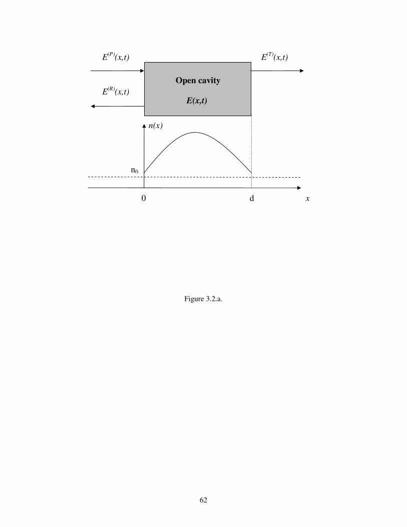
62
Figure 3.2.a.
Open cavity E(x,t)
x
n(x)
0 d
n0
E(P)(x,t)
E(R)(x,t)
E(T)(x,t)

63
Figure 3.2.b.
Figure 3.2.c.
-3.14
0
3.14
1.0
0 0.5 1.0 1.5 2.0
QNM theoryNumeric methods
ω/ωref
T=t
2 , ϕ=
Arg
[t]
-3.14
0
3.14
1.0
0 0.5 1.0 1.5 2.0
QNM theoryNumeric methods
ω/ωref
T=t
2 , ϕ=
Arg
[t]

64
Table 3.3.a.
-3.14
0
3.14
1.0
0 0.5 1.0 1.5 2.0
QNM theoryNumeric methods
ω/ωref
T=t
2 , ϕ=
Arg
[t]
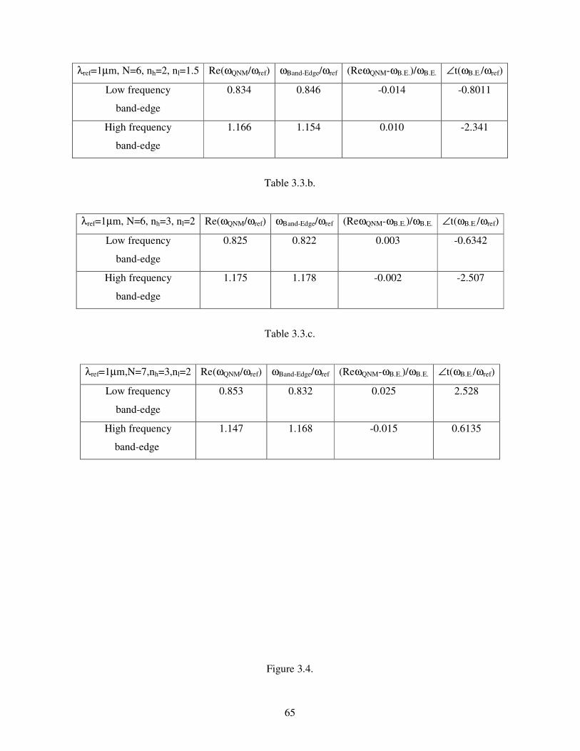
65
λref=1µm, N=6, nh=2, nl=1.5 Re(ωQNM/ωref) ωBand-Edge/ωref (ReωQNM-ωB.E.)/ωB.E. ∠t(ωB.E./ωref)
Low frequency
band-edge
0.834 0.846 -0.014 -0.8011
High frequency
band-edge
1.166 1.154 0.010 -2.341
Table 3.3.b.
λref=1µm, N=6, nh=3, nl=2 Re(ωQNM/ωref) ωBand-Edge/ωref (ReωQNM-ωB.E.)/ωB.E. ∠t(ωB.E./ωref)
Low frequency
band-edge
0.825 0.822 0.003 -0.6342
High frequency
band-edge
1.175 1.178 -0.002 -2.507
Table 3.3.c.
λref=1µm,N=7,nh=3,nl=2 Re(ωQNM/ωref) ωBand-Edge/ωref (ReωQNM-ωB.E.)/ωB.E. ∠t(ωB.E./ωref)
Low frequency
band-edge
0.853 0.832 0.025 2.528
High frequency
band-edge
1.147 1.168 -0.015 0.6135
Figure 3.4.
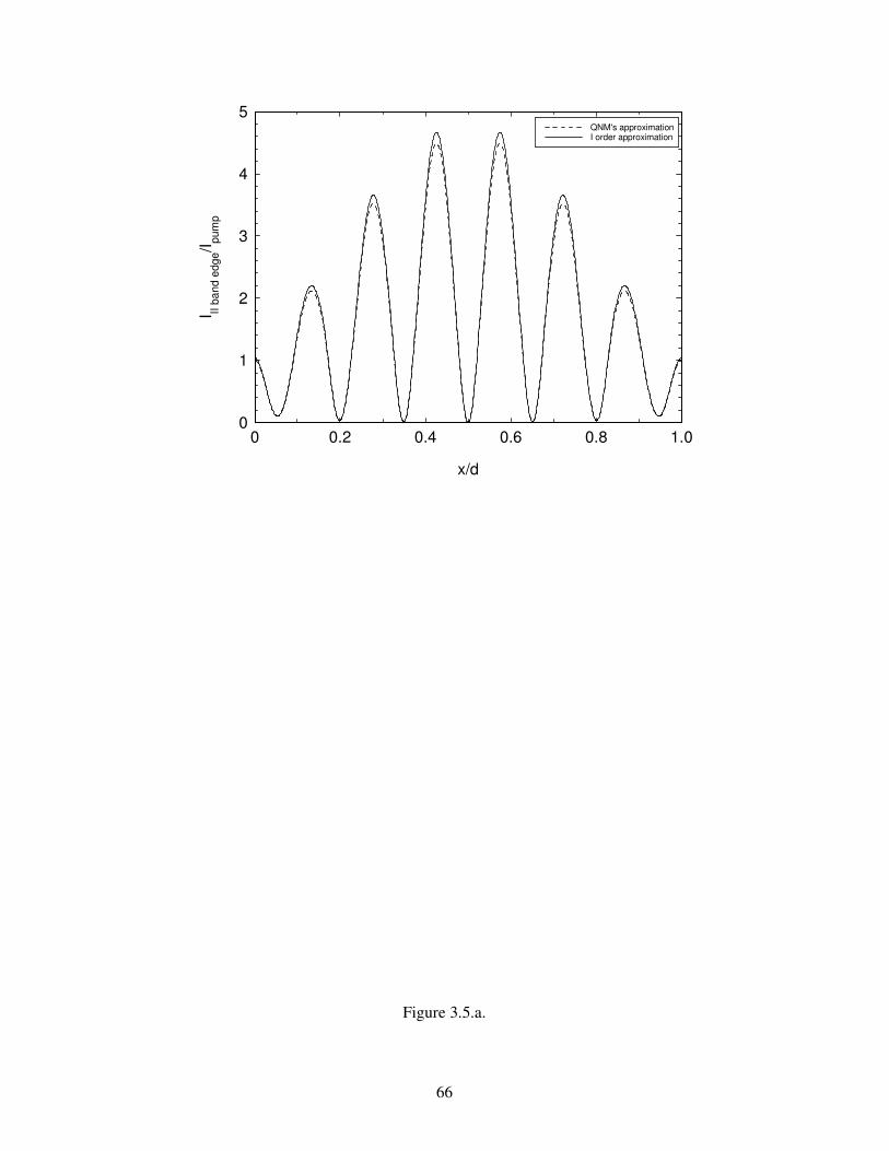
66
Figure 3.5.a.
0
1
2
3
4
5
0 0.2 0.4 0.6 0.8 1.0
QNM's approximationI order approximation
x/d
I II ba
nd e
dge/I pu
mp

67
Figure 3.5.b.
Figure 3.1. A cavity opened at both ends, of length d with a refractive index n(x), excited by a left-pump ( ) ( , )PE x t , satisfying the “incoming wave” condition (3.2.3).
0
1
2
3
4
5
0 0.2 0.4 0.6 0.8 1.0
one field pumptwo field pumps ( ∆ϕ=0 )
x/d
I II ba
nd e
dge/I pu
mp
0
4
8
12
16
0 0.2 0.4 0.6 0.8 1.0
one field pumptwo field pumps ( ∆ϕ=0 )
x/d
I I ban
d ed
ge/I pu
mp

68
Figure 3.2. Transmission spectrum (squared modulus and phase) predicted by Quasi Normal Mode’s (QNM’s) approach (—) and by numeric methods existing in the literature [10] (- - -) , for symmetric QW 1D-PBG structures, with reference wavelength 1ref mλ = µ and: (a) number of
periods 6N = , refractive indices 2, 1.5h ln n= = ; (b) 6N = , refractive indices 3, 2h ln n= = ; (c)
7N = , 3, 2h ln n= = . Table 3.3. Three examples of symmetric QW 1D-PBG structures are considered: (a) λref=1µm, N=6, nh=2, nl=1.5, (b) λref=1µm, N=6, nh=3, nl=2, (c) λref=1µm, N=7, nh=3, nl=2. For each of the three examples, the low and high frequency band-edges are described in terms of their resonances (ωBand-Edge/ωref) and phases ∠t(ωB.E./ωref); besides, there is one QNM’s frequency next to every single band-edge: the real part of the QNM’s frequency Re(ωQNM/ωref) is reported together with the relative shift from the band-edge resonance (ReωQNM-ωB.E.)/ωB.E.. Figure 3.4. With reference to a symmetric QW 1D-PBG structure (λref=1µm, N=6, nh=3, nl=2), the “e.m. mode” intensity III band-edge at the high frequency band edge (ωII band-edge/ωref=1.178), in units of the intensity Ipump for a field pump, is plotted as a function of the dimensionless space x/d, where d is the length of the 1D-PBG structure. It is clear the shifting between the QNM’s approximation (3.3.12) (the field intensity distribution III band-edge is approximated by the QNM’s function corresponding the QNM’s frequency next to the high frequency band-edge) and the first order approximation (3.3.13) (a superior order approximation, the field intensity distribution III band-edge is the product of the same QNM’s function for a weigh coefficient which takes into account the shift between the band-edge resonance and the QNM’s frequency). Figure 3.5. With reference to a symmetric QW 1D-PBG structure (λref=1µm, N=6, nh=3, nl=2), the “e.m. mode” intensities excited inside the open cavity by one field pump (- - -) coming from the left side [see eq. (3.3.13)] and by two counter-propagating field pumps in phase (—) [see (3.3.15)] are compared when each of the two field pumps are tuned in (a) the low frequency band-edge (ωI band-
edge/ωref=0.822) or (b) the high frequency band-edge (ωII band-edge/ωref=1.178). The field intensity distributions II band-edge and III band-edge, in units of the intensity for the two pumps Ipump , are plotted as functions of the dimensionless space x/d, where d is the length of the 1D-PBG structure. So, two counter-propagating field pumps tuned to the same transmission resonance do not necessarily excite the field distribution that one might expect at that frequency if the same field pumps have an appropriate phase-difference.
69
Second Part:
QNM’s approach for open cavities in quantum electrodynamics.
Chapter 4
70
Non canonical Quasi Normal Mode’s Quantization for open cavities.
1. Introductive discussion.
The calculations in quantum optics have traditionally used a form of quantum
electrodynamics in which the e.m. field is assumed to be confined within an optical cavity [1][2].
The e.m. field is quantized in terms of a complete set of discrete eigen-modes of the cavity. When
appropriate boundary conditions are applied at the cavity walls, the discrete modes can have the
form of a standing or running wave. However, the vast majority of optical experiments have no
identifiable cavity, but rather the optical energy flows from sources through some kind of
interaction region to a set of detectors. For systems of this nature, it is preferable to quantize the
electromagnetic field in free space with a set of e.m. modes characterized by a continuous wave
vector [3][4].
Blow et al. have formulated in ref. [5] the quantum theory of optical wave propagation without
recourse to the cavity quantization. This approach avoids the introduction of a box-related mode
spacing and enables to use a continuum frequency space description. Ref. [5] introduces a complete
orthonormal set of operators that can describe states of finite energy. The set is countable and the
operators have all the usual properties of the single-mode frequency operators. With the use of these
operators a generalization of the single-mode normal-ordering theorem is proved. The formalism
presented in ref. [5] is suited to the treatment of quantum optical systems where the propagation
effectively takes place in one dimension with no restriction on the optical length of the one
dimensional axis. Finally it should be emphasized that the removal of the notional cavity is
accomplished without any increase in the mathematical complexity of the formalism.
However, with the advent of modern optical materials, such as optical fibres, the problem of
quantization of the e.m. field in dielectrics has become an important subject and much activity has
been taking place in this field.
In the case of linear conservative dielectrics, the quantization is well-known for systems where the
permittivity (electric permeability) ε is a real constant [1][2]. For inhomogeneous media the
situation is more complicated, because the permittivity is a real function of space, i.e. ( )xε ε= .
Recently two methods have been developed for the quantization of the e.m. field in inhomogeneous
linear dielectrics.

71
The first [referred to as the Langevin noise (LN) method] [6] is based upon the introduction of
Langevin noise current (and charge) densities, as dictated by the fluctuation-dissipation theorem [4],
into the classical Maxwell equations which can then be transferred to quantum theory by conversion
of the field quantities into operators. In this scheme, the dyadic Green’s function associated with the
classical (inhomogeneous) Helmholtz equation plays a prominent role. Its properties come into play
by deriving the equal-time commutators for the e.m. fields, given those of the noise current
operator.
The second [referred to as the auxiliary field (AF) method] [7] also starts off from the classical
Maxwell equations. Here, the introduction of a set of auxiliary fields (instead of a noise current)
allows the replacement of the Maxwell’s equations, which features a time convolution term relating
the polarization to the electric field, by a new set of equations for the combined set of
electromagnetic and auxiliary fields but without time convolutions. The formalism can then be cast
into a Hamiltonian form which, upon quantization, features a noise current with the same
commutation properties as in the LN formalism [8]. For ease of comparison, a generalized temporal
gauge has been adopted, but the actual choice does of course not affect the equal-time commutator.
A third method uses the discrete (dissipative) Quasi Normal Modes (QNMs) of a leaky cavity
rather than the continuous (Hermitian) NMs of universe [1]-[4]; Ho et al. in ref. [2] already
made an essential first step towards the application of QNMs to quantum electrodynamics
phenomema in one side open and homogeneous cavities: the second quantization of the e.m.
field in a leaky cavity is formulated, from first principles, in terms of the QNMs, which are
eigen-solutions of the evolution equation, decaying exponentially in time as the energy leaks to
outside
[1]. The QNM’s method is usually justified in the following way: let the central system [0, ]C d=
(here the open cavity) be described by a Hamiltonian CH and the bath ( ,0) ( , )B d= −∞ ∪ ∞ (the
rest of universe) be described by a Hamiltonian BH , with the two subsystems coupled by an
interaction term IH , C B IH H H H= + + ; the effect of IH is then eliminated and expressed as a
dissipation and a fluctuation force acting on C [11]. There appears to be a novelty in applying such
arguments to problems of the present type, which can be characterized in general as involving leaky
cavity; in fact, the degrees of freedom of C are ( , ) 0 , x t x dφ ≤ ≤ , while those of B are
( , ) 0 , , x t x x dφ < > . The two are coupled not by a term in the Hamiltonian but by boundary
conditions [12]: the Hilbert space of wave functions satisfying the boundary conditions, hence the
subspaces for C and B, “know” about each other through the conditions at the interfaces.

72
In ref. [8], the second quantization scheme based on QNM’s approach has been extended to double
side open and inhomogeneous cavities, excited by vacuum fluctuations of the universe. In ref. [9],
the QNM’s second quantization has been applied to leaky cavities, but excited by two counter-
propagating field pumps. The QNM’s quantization succeeds in incorporating the external pumping
fields tracing back their effect to that of two assigned electrical currents [15] existing only on the
two limiting surfaces of the open cavity; as a consequence, ref. [9] enables to establish, for the first
time, a direct link between the internal QNM’s operators of ref. [2] and the external NM’s ones of
ref. [5] at a generic frequency. Besides, QNM’s commutation rule is not canonical, and it depends
on the geometry of the leaky cavity and the phase-difference of the two pumps; ref. [9] confirms
that the third method of ref. [2] does not obey to canonical commutation rules adopted by the first
and second methods of ref. [6]-[8], so QNM’s method, respect to the other methods, paves naturally
the way to interesting investigations like, for example, the modified density of modes inside the
open cavity [16], as well as the consequent modification of the spontaneous and stimulated
emission processes of an atom placed inside the leaky cavity.
2. Incoming Waves conditions.
The expansion of a classical field sketched in chapter 1 is restricted to outgoing waves: the
linear space Γ of function pairs [ ( , ), ( , )]x t x tφ φ is considered, where the scalar field ( , )x tφ and its
Lagrange conjugate momentum ( , )x tφ is defined on the interval [0, ]C d= of the open cavity; the
two functions ( , )x tφ and ( , )x tφ are differentiable and they satisfy the outgoing waves conditions
(1.2.6). In preparing the ground for the expansion of a quantum field [1]-[4], it is necessary to
remove this restriction, for the simple reason that zero-point quantum fluctuations will inevitably
contain incoming waves as well. Moreover, one would wish that the ensuing theory should be
applicable to situations where there are incoming pump fields.
Thus, the equation (1.2.2) of the scalar field ( , )x tφ is studied for the open cavity [0, ]C d=
together with the outside ‘‘bath,’’ i.e. on the half-lines 0x < and x d> , with relative dielectric
constant 2( ) ( )x n xρ ∝ satisfying the discontinuity and “no tail” conditions
[1]: 0( )xρ ρ= for 0x < and x d> . The initial conditions are now arbitrary and accordingly the
outgoing waves conditions (1.2.6) are abandoned, i.e. the restriction of the scalar field to the open
cavity need not lie in the linear space Γ . As in ref. [2], the expansion formula [see eqs. (1.2.1) and
(1.2.11)], and the inner product definition and notation [see eq. (1.3.4)] are retained even though
[ ( , ), ( , )]x t x tφ φ ∉Γ . The sum for the first component converges to ( , )x tφ everywhere, while the
73
sum for the second component converges to ( , )x tφ everywhere except at 0x = and x d= . This
flaw on a set of measure zero does not lead to problems, however, for the projection formula
(1.2.11) renders the coefficients ( )na t well defined irrespective of the convergence of the series for
( , )x tφ and ( , )x tφ .
2. 1. Extending QNM’s approach:
e.m. problem of an open cavity excited
by two classical counter-propagating incoming waves.
In this section, the QNM’s approach is extended to solve the e.m. problem of two classical
counter-propagating waves exciting an open cavity; this theoretical extension, here reported, has
been presented in ref [9]. The idea of counter-propagating field pumps is schematically reported in
fig. 4.1; an open cavity of length d, filled with a medium having refractive index ( )n x , is excited by
two field pumps which obviously have to satisfy the field equation (1.2.2): the first one, denoted as ( ) ( , )x tφ → , travels in the positive x direction and enters the cavity from the left side, whereas the
second one ( ) ( , )x tφ ← , in the negative x direction, enters the cavity from the right side.
The two pumps ( ) ( , )x tφ → and ( ) ( , )x tφ ← satisfy some boundary conditions, defined incoming wave
conditions
( ) ( )
0
( ) ( )0
( , ) ( , ) for 0
( , ) ( , ) for
x t
x t
x t x t x
x t x t x d
φ ρ φ
φ ρ φ
→ →
← ←
∂ = − ∂ <
∂ = ∂ >
, (4.2.1)
where 20 0( / )n cρ = and 0n is the outside refractive index. Owing to the theorem of equivalence for
the e.m. sources [15], the two real pumps in the free space can be substituted by two fictitious
electrical currents on the surfaces of the cavity:
( ) ( )
0 0 00
( ) ( )0 0
( ) 2 ( , ) 2 (0, )
( ) 2 ( , ) 2 ( , )
x tx
d x tx d
J t x t t
J t x t d t
ρ φ ρ φ
ρ φ ρ φ
→ →
=
← ←
=
= − ∂ = ∂
= ∂ = ∂
. (4.2.2)
So, respect to ref. [2] , the fictitious electrical currents on the surfaces of the open cavity have been
now justified. The advantage of this replacement is the possibility to develop the QNM’s approach
only into the spatial domain [0, ]C d= , including the driving sources now traced back to the two
currents on the surfaces of the cavity. In such driven situation, the boundary conditions associated
to the equation (1.2.2) of the scalar field, first expressed by the outgoing waves conditions (1.2.6),
now can be cast in the following form:

74
0 0
0
( , ) ( , ) ( ) for 0
( , ) ( , ) ( ) for
x t
x t d
x t x t J t x
x t x t J t x d
φ ρ φ
φ ρ φ
∂ − ∂ = =
∂ + ∂ = =
. (4.2.3)
The refractive index ( )n x of the open cavity satisfies the discontinuity and no-tail conditions
[1], so, inside the cavity, the QNM’s functions form an orthogonal basis [2] and the scalar field can
be calculated as a superposition of QNMs
*
0
( , ) ( ) ( ) [ ( ) ( ) ( ) ( )]n n n n n nn n
x t a t F x a t F x a t F xφ∞ ∞
∗
=−∞ == = + , (4.2.4)
where are introduced the normalized QNM’s functions ( ) ( ) 2n n nF x f x= ω n nf f , denoting the
QNM’s norm as n nf f . The coefficients )(tan of the QNM’s superposition satisfy the dynamic
equation:
00
( ) ( ) [ (0) ( ) ( ) ( )]2
n n n n n d
n
ia t i a t F J t F d J tω
ω ρ+ = + . (4.2.5)
In this new scenario, it is easy to verify that the QNM’s coefficients ( ) (0)exp( )n n na t a i tω= − , in
absence of an external pumping [see eq. (1.2.12)], can be deduced as a particular case of eq. (4.2.5),
imposing 0 ( ) ( ) 0dJ t J t= = . The symmetry property ( ) ( )n na t a t∗− = [see eq. (1.2.12)] holds also in
presence of counter-propagating pumps, as it can be easily observed from eq. (4.2.5), reminding
that 0 ( )J t and ( )dJ t are real functions. From a simple inspection of eq. (4.2.5), all the coefficients
( )na t are driven by the two currents 0 ( )J t and ( )dJ t ; even if each coefficient has the property
0)Im( <nω , the incoming waves conditions (4.2.3) ensure the presence of quasi-stationary regime
solutions. The coupling between the QNMs inside the cavity and the currents 0 ( )J t and ( )dJ t is
determined by the surface values of the QNM’s functions (0)nF and ( )nF d . So, the Fourier’s
transform with a real frequency,
[ ] [ ]1exp( )
2i t dtω
π
∞
−∞
ℑ = , (4.2.6)
can be applied to eqs. (4.2.4)-(4.2.5) and (4.2.2) . If the two pumps in the free space are tuned at the
frequency , the scalar field inside the cavity is
*
0
( ) ( ) ( ) [ ( ) ( ) ( ) ( )]n n n n n nn n
x a F x a F x a F xωφ ω ω ω∞ ∞
∗
=−∞ == = + , (4.2.7)
where
0
0
(0) ( ) ( ) ( )( )
2 ( )n n d
n
n n
F J F d Ja
ω ωωρ ω ω ω
+=−
, (4.2.8)
75
being
( ) ( )
0 0 00
( ) ( )0 0
( ) 2 ( ) 2 ( ) (0)
( ) 2 ( ) 2 ( ) ( )
x x
d x x d
J x i
J x i d
ω ω
ω ω
ω ρ φ ρ ω φ
ω ρ φ ρ ω φ
→ →
=
← ←
=
= − ∂ = −
= ∂ = −
. (4.2.9)
3. Second quantization.
Having outlined, in the previous section, necessary aspects of the classical QNM’s approach,
let turn now to the quantum description of the e.m. field inside and outside an open cavity under
incoming waves conditions of two counter-propagating pump fields. In this section, the second
quantization of e.m. field in its simplest kind is applied, being described classically by one Lorentz
invariant quantity [1] at each space-time point.
In what follows, let report schematically some necessary definitions about the so called scalar
fields. The scalar field can be described by an action which is defined as the time integral of a
Lagrangian. The Lagrangian density L is a function of the space-time point (x,t) through its
dependence on the scalar field ( , )x tφ and its derivatives xφ∂ and tφ∂ . The Lagrangian for the field
equation [see eq. (1.2.2)] is calculated as:
2 2( , ) ( )( ( , )) ( ( , )) 2t xL x t x x t x tρ φ φ = ∂ − ∂ . (4.3.1)
A canonical momentum of the scalar field ( , )x tφ can be defined, in analogy to the systems with a
finite number of degrees of freedom, as
( , )( )t
Lx t
δφδ φ
=∂
, (4.3.2)
and (see ref. [8]) it is calculated as an immediate consequence of its definition (4.3.2)-(4.3.1),
( , ) ( ) ( , )tx t x x tφ ρ φ= ∂ , (4.3.3)
i.e. the product of the refractive index (x) and the time derivative tφ∂ of the scalar field.
An Hamiltonian density h(x,t) can be introduced, so that the integral of h(x,t) is the total
Hamiltonian H(t). The Hamiltonian density h(x,t) can be defined in terms of the canonical momenta
as
( , ) ( , ) ( , ) ( , )th x t x t x t L x tφ φ= ∂ − , (4.3.4)
so the total Hamiltonian H(t) is
( ) ( , )H t h x t dx∞
−∞
= . (4.3.5)

76
The Hamiltonian density (4.3.4) associated to the Lagrangian (4.3.1) and the canonical momentum
(4.3.3) is calculated as
[ ] [ ]2 2
( , ) ( , )( , ) ( )
2 2x tx t x t
h x t xφ φ
ρ∂ ∂
= + . (4.3.6)
As discussed in [2], the total Hamiltonian is time-independent, whether it satisfies the
Sommerfeld’s radiative conditions [15] of the free space or the boundary conditions of an open
cavity with narrow resonances, i.e. [8]
( )H t H≈ (4.3.7)
in conservative limit |Imn|<<Ren.
For a quantum mechanics treatment, the equal-time canonical quantization rules are adopted
( , ), ( , ) ( )x t x t i x xφ φ δ′ ′ = − , (4.3.8)
where (x) is the Dirac’s delta distribution, being the Planck’s constant. Eq (4.3.8) implies that
( , )x tφ and ( , )x tφ are no more considered as classical scalar fields, but they should be treated as
field operators, denoted as ˆ( , )x tφ and ˆ ( , )x tφ . The quantization procedure is a direct consequence
of the equal-time canonical quantization rules.
3. 1. Canonical commutation rules in free space:
quantum apparatus for counter-propagation of incoming waves.
In this section, the theory of continuum fields in quantum optics [5] is applied to discuss the
e.m. problem of two quantum counter-propagating waves exciting an open cavity; this theoretical
discussion, here reported, has been presented in ref [9].
The electric field operator ( )ˆ ( , )x tφ → associated to a propagation in the positive x direction can be
obtained as
( ) ( ) ( )ˆ ˆ ˆ( , ) ( , ) ( , )x t x t x tφ φ φ→ → →+ −= + , (4.3.9)
where
( ) 1/ 202
0 0 0
ˆˆ ( , ) ( ) ( ) exp( )2
x t i d b g x i tn ωφ ω ρ ω ω ω
ε
∞→
+ = −
(4.3.10)
and, obviously,
( ) ( ) †ˆ ˆ( , ) [ ( , )]x t x tφ φ→ →− += , (4.3.11)
which are respectively called positive and negative part of the electric field operator. As it can be
easily verified, the two quantities alone (4.3.10) and (4.3.11) are not observables. In eq. (4.3.10),

77
0( ) 1 2 exp( )g x i xω π ω ρ= is the Normal Mode’s (NM’s) function, 0ε the dielectric constant in
vacuum and 2h π= , being h the Planck’s constant. The Fourier’s transform (4.2.6) of the field
operator (4.3.9) can be expressed as
( ) 1/ 20 02
0 0
ˆˆ ( ) ( ) exp( )2
x i b i xnωφ ρ ω ω ω ρ
ε→ =
, (4.3.12)
satisfying, as property,
( ) ( ) †ˆ ˆ( ) [ ( )]x xω ωφ φ→ →− = . (4.3.13)
It is easy to verify that the operator (4.3.12) satisfies the incoming wave condition in quantum
domain:
( ) ( )0
ˆ ˆ( ) ( )x x i xω ωφ ω ρ φ→ →∂ = . (4.3.14)
In the context of the problem examined in this section, eq. (4.3.12) defines an incoming wave, left
to right (LTR) propagating, in the zone 0x < .
The electric field operator ( )ˆ ( , )x tφ ← associated to the propagation in the opposite direction, can be
obtained applying the parity operator π [2] to eqs. (4.3.9)-(4.3.11); the electric field operator
propagating in the negative x direction is
( ) † ( ) ( )ˆ ˆ ˆ( , ) ( , ) ( , )x t x t x tφ π φ π φ← → →= = − . (4.3.15)
Applying the parity operator π to eq. (4.3.12), the Fourier’s transform (4.2.6) of the field operator
(4.3.12) can be expressed as
( ) 1/ 20 02
0 0
ˆˆ ( ) ( ) exp( )2
x i b i xnωφ ρ ω ω ω ρ
ε← = −
, (4.3.16)
satisfying, as property,
( ) ( ) †ˆ ˆ( ) [ ( )]x xω ωφ φ← ←− = . (4.3.17)
By construction, the operator (4.3.16) satisfies the incoming wave condition in quantum domain:
( ) ( )0
ˆ ˆ( ) ( )x x i xω ωφ ω ρ φ← ←∂ = − . (4.3.18)
Eq. (4.3.18) is valid for all x values but, in the context of the problem examined in this section, it
defines an incoming wave, right to left (RTL) propagating, in the zone x d< .
In all the observables introduced, the NM’s annihilation and creation operators, respectively ˆ( )b ω
and †ˆ ( )b ω , satisfy the canonical commutation rules:
†ˆ ˆ[ ( ), ( )] ( )b bω ω δ ω ω′ ′= − . (4.3.19)
One possible experimental apparatus realizing the incoming waves conditions (4.3.14) and
(4.3.18) of two counter-propagating field pumps is shown in fig. 4.2. The fifty-fifty beam splitter BS
78
splits an input field ( )ˆ ( , )in x tφ in two output fields, the LTR propagating field pump ( )ˆ ( , )x tφ → and
the auxiliary field ( )ˆ ( , )aux x tφ ; after a spatial translation and inversion, the auxiliary field ( )ˆ ( , )aux x tφ
gives rise to the RTL propagating field pump ( )ˆ ( , )x tφ ← . This is a possible unitary transformation to
realize a quantum counter-propagation of incoming waves. In the quantum domain, the effect of
noise incoming from the other input of beam splitter BS can not be neglected; so, another input field
( )ˆ ( , )noise x tφ must be considered.
As a quantum model of the beam splitter BS, a generic version of the 50/50 beam splitter is
considered with a SU(2) transfer matrix [2], i.e.
11
12
i
i
eB
e
ϕ
ϕ
∆
− ∆
−=
, (4.3.20)
where ϕ∆ is regarded as the preponderant term, due to the beam splitter BS, of the phase difference
between the two counter-propagating field pumps, on the surfaces of the open cavity. The transfer
matrix (4.3.20), if 2ϕ π∆ = − , becomes the usual one, i.e.11
12
i
i
. So, the expression for the
Fourier transform of the LTR field pump ( )ˆ ( )xωφ → , entering the cavity from the left side, is given by
the following relation:
( ) 1/ 20 02
0 0
ˆ ˆ( ) ( )exp( )ˆ ( ) exp( )2 2
noiseb b ix i i x
nωω ω ϕφ ρ ω ω ρ
ε→ − ∆=
, (4.3.21)
where ˆ ( )noiseb ω is the noise field operator, satisfying the canonical commutation relation (4.3.19).
The auxiliary field ( )ˆ ( , )aux x tφ , outgoing from the beam splitter BS, is spatially translated by a
system of mirrors (fig. 2.4.). From an operator point of view, these processes can be viewed as an
application of two unitary transformations on the field ( )ˆ ( , )aux x tφ : the first one transformation,
indicated by dT , induces a spatial translation of the cavity length d, whereas the second one, π,
makes a spatial inversion; summarizing, the RTL field pump ( )ˆ ( , )x tφ ← can be viewed as
† † ( )ˆ ( , )π φ πauxd dT x t T [2]. In order to point out the role of the beam splitter BS which introduces the
degree of freedom , the phase term due to the propagation of the auxiliary field ( )ˆ ( , )aux x tφ is
regarded negligible respect to the phase term due the beam splitter BS, i.e. <<. So, the
Fourier’s transform of the RTL field pump ( )ˆ ( )xωφ ← , entering the cavity from the left side, is given
by:

79
( ) 1/ 20 02
0 0
ˆ ˆ( ) exp( ) ( )ˆ ( ) exp[ ( )]2 2
noiseb i bx i i x d
nωω ϕ ωφ ρ ω ω ρ
ε← − ∆ += − −
. (4.3.22)
Concluding this subsection, it is possible to affirm that, using a set-up as the one reported in fig. 2.4,
it is possible to obtain, as inputs of the open cavity, two counter-propagating field pumps ( )ˆ ( )xωφ →
and ( )ˆ ( )xωφ ← mismatched with a phase-difference , respectively represented by the operators
(4.3.21)-(4.3.22) and satisfying the incoming waves conditions (4.3.14) and (4.3.18).
3. 2. Non canonical QNM’s commutation rules in an open cavity:
link of QNM’s operators inside the cavity with NM’s operators of the free space.
Let purpose to develop a formalism whereby second quantization of the scalar field ( , )x tφ
can be implemented in terms of the discrete QNMs [see eq. (4.2.4)], such that the coefficients ( )na t
and ( )na t∗ of the QNM’s superposition can be interpreted respectively as generalized annihilation
and creation operators of the QNMs. In analogy with the canonical quantum expansion of scalar
fields in the free space, where NM’s operators are multiplied by NM’s functions [2], second
quantization on the field expansion (4.2.4) proceeds first by promoting the scalar field ( , )x tφ to a
field operator denoted as ˆ( , )x tφ , so that the superposition coefficient ( )na t and ( )na t∗ can be
promoted as well as QNM’s operators, ˆ ( )na t and †ˆ ( )na t , multiplying QNM’s functions. The e.m.
field ˆ( , )x tφ can be regarded as an operator only in the open cavity (see ref. [9]), and the QNM’s
operators ˆ ( )na t and †ˆ ( )na t obey the operator form of the motion equation (4.2.5).
The field operator ˆ ( )xωφ , which in Fourier’s domain satisfies the property †ˆ ˆ( ) ( )x xω ωφ φ−= , is
expressed as a superposition of the QNM’s operators ˆ ( )na ω in “(frequency) Heisenberg’s
representation”, i.e.
†
0
ˆ ˆ ˆ ˆ( ) ( ) ( ) [ ( ) ( ) ( ) ( )] , 0ωφ ω ω ω∞ ∞
∗
=−∞ == = + ∀ ≤ ≤ n n n n n n
n n
x a F x a F x a F x x x d , (4.3.23)
and the QNM’s operators have to satisfy the property † ( ) ( )n na aω ω−= − , which is similar to the
expression valid for NM’s operators. If the equal-time canonical quantization rule (4.3.8) is applied,
the QNM’s commutation relation can be derived in absence of an external pumping or in presence
of two counter-propagating incoming waves [9].

80
Consider an open cavity in absence of an external pumping. If the equal-time canonical
quantization rule (4.3.8) is applied, the commutation relation for the QNM’s operators ˆna and †ˆna is
derived (see ref. [8])
†2
Re[ ]ˆ ˆ,2 1/
n nn n
n
Ia a
dω
ω =
, (4.3.24)
where are introduced the overlapping integrals [8]:
2 2 20
0
1( ) ( ) (0) ( )
2 Im
d
n n n nn
dI x F x dx F F d
d
ρρ
ω = = + . (4.3.25)
Eqs. (4.3.24) and (4.3.25) confirm that the operators na and †na can be interpreted as generalized
annihilation and creation operators of the QNMs. In fact, in the conservative limit [2], the leaky
cavity is characterized by narrow resonances |Imωn|<<|Reωn|; since the damping is related to the
escape of energy from the two surfaces of the cavity, in eq. (4.3.25) the imaginary part Im[ωn]0
vanishes with the same velocity of 2 20 / 2( (0) ( ) ) 0n nF F dρ + → and each overlapping integral
(4.3.25) tends to In1/d. As a consequence, the QNM’s commutator becomes †ˆ ˆ, 2n n na a ≅ ω ,
similar to the one concerning the annihilation and creation operators, nb and †nb , of a closed cavity,
if ˆˆ 2( / )n n na b= ω and † †ˆˆ 2( / )n n na b= ω are assumed.
In absence of an external pumping, the equations of motion (4.2.5) for the QNM’s operators, in
quantum domain, read as
† †
ˆ ˆ( ) exp( )
ˆ ˆ( ) exp( )n n n
n n n
a t a i t
a t a i t∗
= − ω
= ω, (4.3.26)
which in Fourier’s domain become:
† †
ˆ ˆ( ) 2 ( )
ˆ ˆ( ) 2 ( )n n n
n n n
a a
a a ∗
ω = πδ ω − ω
ω = πδ ω + ω. (4.3.27)
So, the QNM’s operators are not observables, because satisfy the symmetry conditions †ˆ ˆ ˆ( ) ( ) ( )n n na a a−ω = −ω ≠ −ω , and the QNM’s commutation relation in “(frequency) Heisenberg’s
representation” becomes:
† †ˆ ˆ ˆ ˆ( ), ( ) 2 , ( ) ( )n n n n n na a a a ∗′ ω ω = π δ ω − ω δ ω + ω . (4.3.28)
Consider a leaky cavity [0, ]C d= excited by two counter-propagating field pumps ( )ˆ ( )xωφ →
and ( )ˆ ( )xωφ ← , mismatched with a phase-difference (see fig 4.2.), respectively represented by the
operators (4.3.21)-(4.3.22) and satisfying the incoming waves conditions (4.3.14) and (4.3.18). The

81
quantum principle of correspondence [2] can be applied, in frequency domain, to the two fictitious
electrical currents (4.2.9) on the surfaces of the open cavity, i.e.
( )
0 0
( )0
ˆˆ ( ) 2 ( ) (0)ˆˆ ( ) 2 ( ) ( )d
J i
J i d
ω
ω
ω ρ ω φ
ω ρ ω φ
→
←
= −
= −, (4.3.29)
so, reminding eqs. (4.3.21) and (4.3.22), the operators corresponding to the two currents on the
surfaces of the cavity result
0ˆ ˆˆ ( ) [ ( ) ( ) exp( )]ˆ ˆˆ ( ) [ ( ) exp( ) ( )]
noise
d noise
J K b b i
J K b i b
ω
ω
ω ω ω ϕ
ω ω ϕ ω
= − ∆
= − ∆ +, (4.3.30)
where is introduced the scalar constant 2 30 0 0 0( )K nω ε ρ ω ρ= . Promoting in operator form eq.
(4.2.8), the QNM’s operators are obtained in (frequency) “Heisenberg’s representation”
0ˆ ˆˆ ( ) ( ) ( ) ( ) ( )ω ω ω ω ω= +n n n da A J B J , (4.3.31)
where ( )nα ω and ( )nb ω are two complex functions in frequency:
0 0
(0) ( )( ) , B ( )
2 ( ) 2 ( )ω ω
ρ ω ω ω ρ ω ω ω= =
− −n n
n n
n n n n
F F dA . (4.3.32)
The link (4.3.31) between the internal QNM’s operator ˆ ( )na ω and the external canonical NM’s
operators ˆ( )b ω and ˆ ( )noiseb ω turns out to be useful when one is interested to evaluate expectation
values for the e.m. field inside an open cavity, since, by using eqs. (4.3.31) and (4.3.30), one can
perform all the average operations over the NMs of the free space.
If the leaky cavity [0, ]C d= presents a refractive index ( )n x satisfying the symmetry properties
( / 2 ) ( / 2)n d x n x d− = + , on the surfaces 0x = and x d= of the open cavity the values of the
QNM’s functions ( )nF x are such that ( ) ( 1) (0)nn nF d F= − . In this hypothesis, the two complex
functions (4.3.32) satisfy the symmetric property:
( ) ( 1) ( )ω ω= − nn nB A . (4.3.33)
Inserting eq. (4.3.30) in eq. (4.3.31) and reminding eq. (4.3.33), it results [9]:
ˆ ˆˆ ( ) ( ) ( )[1 ( 1) exp( )] ( )[1 ( 1) exp( )]ωω ω ω ϕ ω ϕ= + − − ∆ − − − − ∆n nn n noisea K A b i b i . (4.3.34)
Eq. (4.3.34) establishes the link between the QNMs inside a symmetric cavity and the NMs of the
free space. In the particular case 2ϕ π∆ = (or multiple), eq. (4.3.34) becomes:
ˆ2 ( ) ( ) for 0, 2,
ˆ ( )ˆ2 ( ) ( ) for 1,3,
ω
ω
ω ωω
ω ω
== − =
nn
n noise
K A b na
K A b n. (4.3.35)

82
As from eq. (4.3.35), the even QNM’s operators are influenced only by the input field ( )ˆ ( )in xωφ of
the beam splitter BS, whereas in the odd QNMs there is information about the noise field ( )ˆ ( )noise xωφ .
Applying eq. (4.3.34), the commutation rule involving the QNM’s operator ˆ ( )na ω and †ˆ ( )na ω of a
symmetric cavity can be calculated, obtaining:
2† 2ˆ ˆ[ ( ), ( )] 2 ( ) ( 1) cos( ) ( )ωω ω ω ϕ δ ω ω′ ′= − ∆ −nn n na a K A . (4.3.36)
If the leaky cavity is pumped by two counter-propagating incoming waves, the QNM’s
commutation relation is not canonical and depends on the geometry of the open cavity and the
phase difference of the two incoming waves. Modification of the commutation relations with
respect to the canonical ones, gives rise to a modification of the emission properties of the atom
embedded in the cavity, as clearly described in the work of Ueda et al. [16]; therefore, an influence
is expected on the emission processes due to the geometry of the cavity and the phase difference of
the two incoming waves.
3. 3. Auto-correlation function of e.m. field inside an open cavity
as QNM’s superposition depending on the incoming waves.
At a time t>0, the quantum state of an e.m. field is defined by specifying a ket ( )tψ
belonging a state space [2]. The time evolution of the state vector ( )tψ is governed by the
Schroedinger equation
ˆ( ) ( )d
i t H tdt
ψ ψ= , (4.3.37)
where, for the quantum principle of correspondence, the classical total Hamiltonian (4.3.7) is
promoted to a quantum operator H associated with the total energy of the e.m. field. Since the
QNM’s operators are linked to the NM’s ones [see eq. (4.3.34)], in order to calculate the auto-
correlation function of an e.m. field inside an open cavity, it is convenient to calculate the
expectation values on the NMs of the free space, which are well known from canonical quantum
electrodynamics.
In the free space, two counter-propagating field pumps with a phase-difference ϕ∆ (see fig.
4.2.), respectively represented by the operators (4.3.21)-(4.3.22) and satisfying the incoming waves
conditions (4.3.14) and (4.3.18), are tuned at frequency ω and prepared in a quantum state
0 ( ),0ωψ β ω= , (4.3.38)

83
if the beam splitter BS is excited by an input field ( )ˆ ( )in xωφ lying on a coherent state ( )β ω of
amplitude ( )β ω and the noise field ( )ˆ ( )noise xωφ lies on the vacuum fluctuations 0ω . The
expectation values for the NM’s annihilation and creation operators ˆ( )b ω and †ˆ ( )b ω must be
calculated on the initial state (4.3.38). As a consequence, the expectation values of the photon-
number and Hamiltonian operators are respectively
†0 0
ˆ ˆˆ ( ) ( ) ( )N b bω ψ ω ω ψ= (4.3.39)
and
ˆ ˆ( ) ( )H Nω ω ω= . (4.3.40)
Adopting the (frequency) Heisenberg’s representation, the quantum variances of the two current
operators (4.3.30) on the initial state (4.3.37) are operatively defined as
† †0 0 0 0 0 0
ˆ ˆ ˆ ˆ( ) ( ) ( ) ( )J J J Jω ω ψ ω ω ψ= , † †0 0
ˆ ˆ ˆ ˆ( ) ( ) ( ) ( )d d d dJ J J Jω ω ψ ω ω ψ= , (4.3.41)
which can be calculated as [9]:
† † 30 0 0 02
0 0
ˆ ˆ ˆ ˆ ˆ( ) ( ) ( ) ( ) ( ) ( )d dJ J J J Nn
ω ω ω ω ρ ω ρ ωε
= = . (4.3.42)
The quantum cross-correlations of these two current operators, calculated on the initial state, show
the properties [9]:
† † †0 0 0 0
ˆ ˆ ˆ ˆ ˆ ˆ( ) ( ) ( ) ( ) ( ) ( ) ( )d dJ J J J J J exp iω ω ω ω ω ω ϕ∗
= = ∆ . (4.3.43)
In order to model vacuum fluctuations of the free space, the ground state 0 0 ,0ω ω= ,
corresponding to ( ) 0β ω = , is not filled of photons, i.e.
0
ˆ ( ) 0Nβ
ω=
= , (4.3.44)
but its zero of energy must be redefined [2] respect to eq. (4.3.40):
0
ˆ ( ) 2Hβ
ω ω= . (4.3.45)
As a consequence, the two current operators (4.3.30) can be still characterized by the quantum
cross-correlations (4.3.43)-(4.3.42), i.e.
† † 30 0 0 02
0 0
ˆ ˆ ˆ ˆ ˆ( ) ( ) ( ) ( ) ( ) ( ) ( )d dJ J J J N exp in
ω ω ω ω ρ ω ρ ω ϕε
∗= = ∆
, (4.3.46)
since, in hypothesis of vacuum fluctuations, i.e. 0
ˆ ( ) 0Nβ
ω=
= , the two currents can be retained
uncorrelated, i.e. † †0 00 0
ˆ ˆ ˆ ˆ( ) ( ) ( ) ( ) 0d dJ J J Jβ β
ω ω ω ω= =
= = . Then, the quantum variances of the two
current operators must be calculated as

84
( )0† † 20 0 02 0
0 0
ˆ ˆ ˆ ˆ ˆ ˆ( ) ( ) ( ) ( ) ( ) ( ) ( )d dJ J J J N Hn β
ρω ω ω ω ρ ω ω ω ω
ε == = + , (4.3.47)
since, in hypothesis of vacuum fluctuations, i.e. 0
ˆ ( ) 0Nβ
ω=
= , the variances of the two currents
must be retained non-null, i.e. † †0 00 0 0
ˆ ˆ ˆ ˆ ˆ( ) ( ) ( ) ( ) ( )d dJ J J J Hβ β β
ω ω ω ω ω= = =
= ∝ .
The open cavity is excited by two counter-propagating field pumps, respectively represented
by the operators (4.3.21)-(4.3.22), in the initial state (4.3.38). So, the expectation values of the
QNM’s operators can be directly calculated on the initial state (4.3.38). Applying the method of ref.
[2], the auto-correlation function of the e.m. field inside an open cavity can be calculated as a
QNM’s superposition depending on the incoming waves [9]
†0 0
†0 0
0
†
0
ˆ ˆ ˆ ˆ( , , ) ( ) ( ) ( ) ( )
(0) (0) ( ) ( )ˆ ˆ ( ) ( )4 ( )( )
( ) ( ) ( ) ( )ˆ ˆ ( ) ( )4 ( )
ω ω ω ωω ψ φ φ ψ φ φ
ω ωρ ω ω ω ω ω ω
ω ωρ ω ω ω ω
−
∞ ∞′ ′
′=−∞ =−∞ ′ ′
′ ′
′
′ ′ ′Φ = = =
′= +
− +′
+−
n n n n
n n n n n n
n n n nd d
n n n
x x x x x x
F F F x F xJ J
F d F d F x F xJ J
†0
0
†0
0
( )
(0) ( ) ( ) ( )ˆ ˆ ( ) ( )4 ( )( )
( ) (0) ( ) ( )ˆ ˆ ( ) ( )4 ( )( )
ω ω
ω ωρ ω ω ω ω ω ω
ω ωρ ω ω ω ω ω ω
∞ ∞
′=−∞ =−∞ ′
∞ ∞′ ′
′=−∞ =−∞ ′ ′
∞ ∞′ ′
′=−∞ =−∞ ′ ′
++
′+ +
− +′
+− +
n n n
n n n nd
n n n n n n
n n n nd
n n n n n n
F F d F x F xJ J
F d F F x F xJ J
, (4.3.48)
where, in previous calculations, the property †0 / 0 /
ˆ ˆ( ) ( )d dJ Jω ω= − is used for the current operators.
4. Discussion and conclusions.
This chapter has examined the properties of a one-dimensional (1D) size-limited optical
cavity, subjected to two quantized counter propagating field pumps entering through the two
limiting surfaces of the optical device. The interest is strategically confined to the behaviour of the
leaky cavity in its own and then the environmental field pumps are regarded as assigned external
sources acting upon the optical structure under scrutiny. From a mathematical point of view, this
target has been addressed exploiting the Quasi Normal Modes’s (QNM’s) approach in a second
quantization scheme, here appropriately extended with the aim of covering the treatment of an open
cavity coherently pumped by noisy field pumps. It is shown that the presence of such pumps may be
globally taken into account by introducing a new physically transparent description of the boundary
conditions fulfilled by the e.m. field inside the cavity. This chapter succeeds in incorporating the
external counter propagating field pumps tracing back their effect to that of two assigned electrical
85
currents existing only on the two limiting surfaces of the leaky cavity. This method enables to
establish, for the first time, a direct link between the internal QNM’s operators and the external
Normal Mode’s (NM’s) ones at a generic frequency. The advantage of such kind of relations stems
from the possibility of tracing back the calculation of the expectation value of any field operator
inside a open cavity to that involving only field operators of free space. In particular, this route has
been followed in order to get the expression of the auto-correlation function of the e.m. field inside
the cavity. The main result of this chapter, beside the introduction of a peculiar language directly
stemming from the fact of considering such a optical device as a forced open quantum system, is the
understanding of the changes provoked by the two field pumps on some optical properties of the
device. Such studies pave the way to other interesting investigations like, for example, the modified
density of states inside the optical structure, as well as the consequent modification of the
spontaneous and stimulated emission processes of an atom placed inside the structure. In order to
explore the usefulness of these ideas and mathematical approach in a physical context of theoretical
and applicative interest, the optical device can be specialized as a 1D Photonic Band Gap (PBG) of
finite length.
References.
[1] A. Lahiri, P. B. Pal, A first book of Quantum Field Theory (CRC Press, Calcutta, 2000); C.
Cohen-Tannoudji, J. Dupont-Roc, G. Grynberg, Photons and Atoms – Introduction to Quantum
Electrodynamics (John Wiley, New York, 1997).
[2] J. J. Sakurai, Advanced Quantum Mechanics (Addison-Wesley, New York, 1995); S. Weinberg,
The Quantum Theory of Fields (Cambridge University Press, New York, 1996).
[3] L. Mandel, E. Wolf, Optical Coherence and Quantum Optics (Cambridge University Press,
Cambridge, 1995).
[4] R. Feynman, Quantum Electrodynamics (Benjamin, New York, 1962).
[5] K.J. Blow, Rodney Loudon, Simon J.D. Phoenix, T.J. Shepherd, Phys. Rev. A 42, 4102 (1990).
[6] T. Gruner and D.-G. Welsch, Phys. Rev. A 53, 1818 (1996); Ho Trung Dung, L. Knöll, and D.
G. Welsch, Phys. Rev. A 57, 3931 (1998); S. Scheel, L. Knöll, and D.G. Welsch, Phys. Rev. A 58,
700 (1998).
[7] A. Tip, Phys. Rev. A 57, 4818 (1998).
[8] A. Tip, L. Knöll, S. Scheel, and D. G. Welsch, Phys. Rev. A 63, 034806 (2001).
[9] K. C. Ho, P. T. Leung, Alec Maassen van den Brink and K. Young, Phys. Rev. E 58, 2965
(1998).
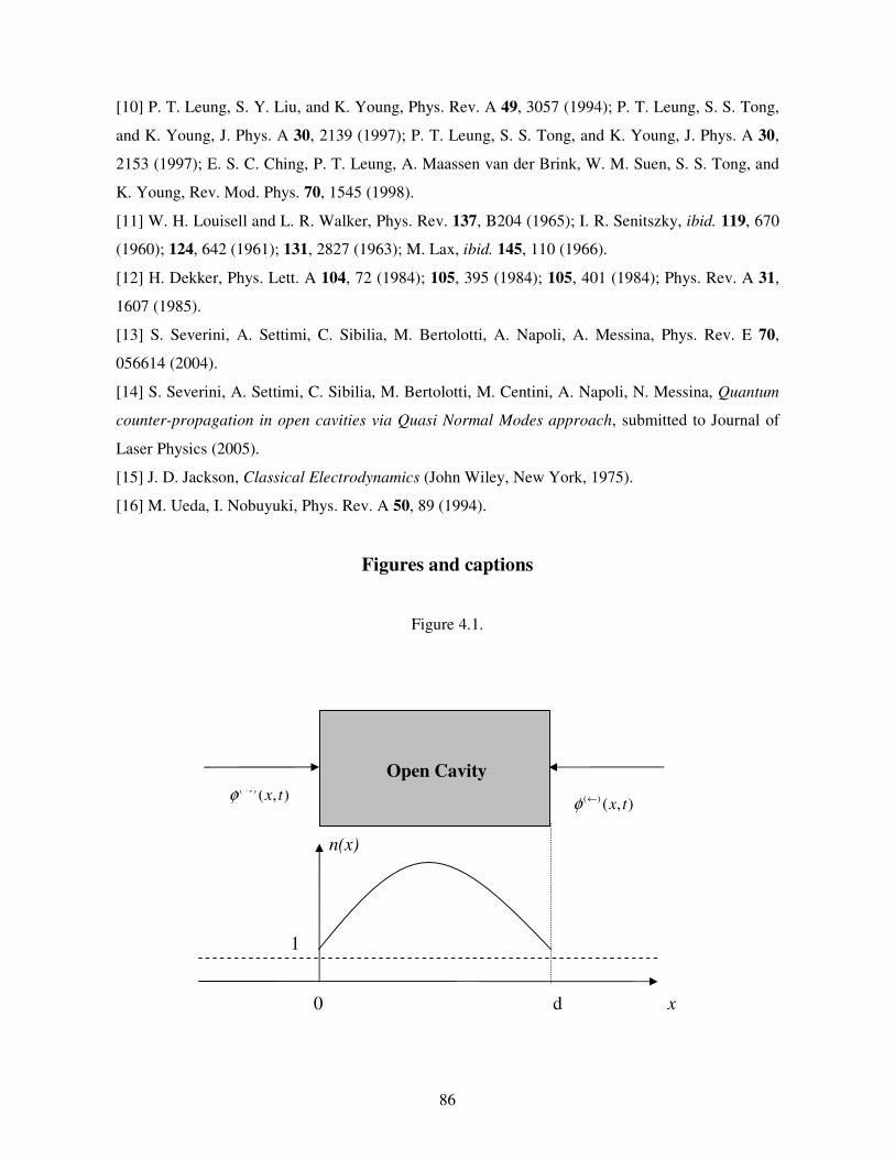
86
[10] P. T. Leung, S. Y. Liu, and K. Young, Phys. Rev. A 49, 3057 (1994); P. T. Leung, S. S. Tong,
and K. Young, J. Phys. A 30, 2139 (1997); P. T. Leung, S. S. Tong, and K. Young, J. Phys. A 30,
2153 (1997); E. S. C. Ching, P. T. Leung, A. Maassen van der Brink, W. M. Suen, S. S. Tong, and
K. Young, Rev. Mod. Phys. 70, 1545 (1998).
[11] W. H. Louisell and L. R. Walker, Phys. Rev. 137, B204 (1965); I. R. Senitszky, ibid. 119, 670
(1960); 124, 642 (1961); 131, 2827 (1963); M. Lax, ibid. 145, 110 (1966).
[12] H. Dekker, Phys. Lett. A 104, 72 (1984); 105, 395 (1984); 105, 401 (1984); Phys. Rev. A 31,
1607 (1985).
[13] S. Severini, A. Settimi, C. Sibilia, M. Bertolotti, A. Napoli, A. Messina, Phys. Rev. E 70,
056614 (2004).
[14] S. Severini, A. Settimi, C. Sibilia, M. Bertolotti, M. Centini, A. Napoli, N. Messina, Quantum
counter-propagation in open cavities via Quasi Normal Modes approach, submitted to Journal of
Laser Physics (2005).
[15] J. D. Jackson, Classical Electrodynamics (John Wiley, New York, 1975).
[16] M. Ueda, I. Nobuyuki, Phys. Rev. A 50, 89 (1994).
Figures and captions
Figure 4.1.
Open Cavity
x
n(x)
0 d
1
( ) ( , )x tφ →
( ) ( , )x tφ ←
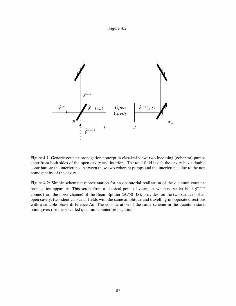
87
Figure 4.2.
Figure 4.1. Generic counter-propagation concept in classical view: two incoming (coherent) pumps enter from both sides of the open cavity and interfere. The total field inside the cavity has a double contribution: the interference between these two coherent pumps and the interference due to the non homogeneity of the cavity. Figure 4.2: Simple schematic representation for an operatorial realization of the quantum counter-propagation apparatus. This setup, from a classical point of view, i.e. when no scalar field ( )noiseφ comes from the noise channel of the Beam Splitter (50/50 BS), provides, on the two surfaces of an open cavity, two identical scalar fields with the same amplitude and travelling in opposite directions with a suitable phase difference . The consideration of the same scheme in the quantum stand point gives rise the so called quantum counter propagation.
Open Cavity
( )ˆ ( , )x tφ → ( )ˆ ( , )x tφ ← ( )ˆ inφ
( )ˆ noiseφ
( )ˆ auxφ
0 d x B

88
Chapter 5
Density of probability for QNMs:
link with boundary conditions of open cavities.
1. Introduction.
Several attempts have been made to generalize the notion of local density of states (LDOS)
and integral density of states (DOS) to the case of open cavities, i.e. structures of finite size where
e.m. energy can flow in and out of the volume bounded by the surface S of the cavity [1]. Quite
surprisingly, the concept of density of states for a finite-size structure still lacks a simple, concise
definition.
If one has a closed cavity such that the e.m. field vanishes at the edges or a cavity where periodic
boundary conditions can be applied (such as a multilayer stack of infinite length), filled with a non-
absorbing medium, one can expect that the e.m. energy will be conserved inside the cavity, and the
problem will be Hermitian. In this case, the LDOS stands for the number of eigen-modes per unit
volume and unit frequency at a point r
inside the cavity. If the e.m. field can be specified by a
single field component (TE or TM polarization), then the scalar Green’s function can be expanded
in terms of the eigen-modes of the cavity and the LDOS can be calculated through the imaginary
part of the scalar Green’s function: ( , ) Im[ ( , , )]r G r rσ ω ω∝ − [2]. The DOS is then defined as the
average LDOS inside the volume V of the cavity.
So one can ask what happens if the cavity is open, such that the e.m. energy can flow in and out of
the volume bounded by the surface S of the cavity. This question has no easy answers
fundamentally because the e.m. problem is no longer Hermitian and the cavity does not admit
eigen-modes in the usual sense of the word.
Structures in which scattering or diffracting elements are arranged in such a way that their
mutual distances are comparable with the wavelength of the incident wave are often referred to as
Photonic Crystals (PCs), or Photonic Band Gap structures (PBGs) [3]-[5].
Although the number of experimental and theoretical reports on 1D-PBG structures is already quite
large, the issue of the DOS, regarding what one means by it, and its true and otherwise implied

89
connections to other physical or measurable quantities, such as emitted energy to name just one, is
still far from being considered closed.
Besides the Green’s function approach [1][2], there are at least other two different approaches to
calculate the DOS which are currently used in literature. The first consists of calculating the DOS as
the spatially averaged e.m. energy density stored inside the 1D-PBG [9]. The second was first
proposed in ref. [10], where the DOS was defined as ( ) (1/ )( / )td d dϕσ ω ϕ ω= , being ( )tϕ ω the
phase of the transmission function ( ) ( ) exp[ ( )]tt t iω ω ϕ ω= .
D’Aguanno et al. have presented in ref. [8] an unified treatment of DOS and tunnelling times in
finite 1D-PBGs. D’Aguanno has exploited connections and differences between the various
approaches used to calculate the DOS, which include the Green function, the Wigner phase time,
and the e.m. energy density, and concludes that the Green function is always the correct path to the
true DOS. Ref. [8] also finds that, for an arbitrary structure, the DOS can always be found as the
ratio between the power emitted by a source located inside the cavity and the power emitted by the
same source in free space, regardless of absorption or dispersion.
Ho et al. in ref. [2] already made an essential first step towards the application of QNMs
[1] to quantum electrodynamics phenomema in one side open and homogeneous cavities. In the
approach of the Normal Modes (NMs) [11], the unit weight of the resonances in the LDOS emerges
simply as a numerical result, and is difficult to understand theoretically; in ref. [2] the same result
(in 1D) is justified analytically, and moreover, one can in principle (a) estimate the corrections due
to other resonances in the LDOS (note that there is no background apart from the QNM’s
contributions) and (b) discuss the local DOS than the integral DOS.
In this chapter, an operative definition is proposed for the DOS of QNMs in a cavity opened from
both ends [9][10], with an inhomogeneous distribution of refractive index [7]-[8]. An appendix
proves the correspondence between the discrete modes of a one-dimensional cavity [2] and the
continuous modes in the absence of a cavity, which approach is formulated in ref. [5]; the physical
link of the DOS with the autocorrelation function of the e.m. field in absence of a cavity is
examined closely. This appendix is viewed as a key passage in order to pave a reasonable way of
generalization: in fact, this kind of link is retained to hold again between the DOS for QNMs and
the autocorrelation function of the e.m. field inside an open cavity.

90
2. “Density” of “states”.
In this section, the density of probability for the Quasi Normal Modes (QNMs) [2]
[1] is operatively defined inside an open cavity which is excited by an external pumping; this
operative definition, here reported, has been presented in refs. [9][10].
The quantum state of an e.m. field, excited inside an open cavity, is generally the super-position of
infinite eigen-states, which are the QNMs. In this sense, a “density” of “states” (DOS) can be
introduced as the density of probability that the e.m. field, excited inside the cavity, is just in one
QNM, oscillating into a range of frequency. As a first step, a local density of states (loc)(x,) can
be introduced. The local DOS of QNMs defines the probability d2p(x,) that an e.m. field, inside an
infinitesimal cavity (x,x+dx), is just in one QNM, oscillating into an infinitesimal range of
frequency (,+d), i.e.
2 ( )( , ) ( , )locd p x x dxdω σ ω ω= . (5.2.1)
The (integral) density of states () remains to define. The (integral) DOS for QNMs is linked to
the probability dp() that an e.m. field, inside a cavity of length d, is just in one QNM, oscillating
into an infinitesimal range of frequency (,+d), i.e.
( ) ( )dp d dω σ ω ω= ⋅ . (5.2.2)
If the geometry of the cavity is represented by the interval C=[0,d], the (integral) DOS for QNMs is
calculated as the spatial average of the local DOS for QNMs inside the cavity, i.e.
( )
0
1( ) ( , )
dloc x dx
dσ ω σ ω= . (5.2.3)
The universe can be viewed as a cavity of infinite length d. The e.m. field inside the
universe is generally a continuum of Normal Modes (NMs) [2][5]. The density of probability that
the e.m. field excited inside the universe is just in the NM tuned at frequency , i.e.
0( ) 1 2 exp( )g x i xω = π ω ρ , is obtained as [2]
2( )0 0( , ) ( ) ( ) 2=loc
ref refx g xωσ ω ρ σ ω ρ π= = , (5.2.4)
where 0=(n0/c)2, being n0 the refractive index of universe and c the light velocity in vacuum.
The (local) DOS of NMs is the ratio between the auto-correlation function of the e.m. field in
the universe and the expectation value of the e.m energy [see Appendix C]. By analogy, let propose
an operative definition of the local QNM’s DOS (loc)(x,) inside an open cavity of relative index
n(x), which is pumped by two counter-propagating field pumps [eqs. (4.3.21) and (4.3.22)]. The
local QNM’s DOS (loc)(x,) is viewed as a n2(x)-modulated transfer function, if the input is the e.m

91
energy ˆ ( )H ω of the two field pumps and the output is the auto-correlation function (x,x,) of
the e.m. field inside the cavity, i.e.
2
( ) 0 ( ) ( , , )( , )
ˆ ( )loc n x x x
x KH
σε ωσ ω
π ω , (5.2.5)
being K is a suitable constant of normalization. Eq. (5.2.5) states that the QNM’s DOS for an open
cavity depends from the boundary conditions of the cavity: in fact, as from chapter 4, the
autocorrelation function [eq. (4.3.48)] of the e.m. field inside the leaky cavity depends from the
expectation values [eqs. (4.3.46) and (4.3.47)] of assigned current operators existing only on the
two surfaces of the cavity, which, for the equivalence theorem of the e.m. source [15], are
equivalent to the two actual field pumps incoming from the universe.
If the open cavity is a symmetric quarter-wave (QW) one dimensional (1D) Photonic Band Gap
(PBG) structure [3] with reference frequency ref, number of periods N and length d, then, over the
[0, 2ref) range, 2N+1 QNMs in units of d can be excited [6]; so, the constant K is obtained by the
normalization condition:
2
0
2 1( )
ref Nd
d
ω
σ ω ω += . (5.2.6)
2. 1. Frequencies of QNMs as resonances of DOS.
In this subsection, the physical meaning of QNM’s frequencies is clarified as resonances of
the DOS for an open cavity (see ref. [7]).
Let suppose that the two counter-propagating field pumps describe vacuum fluctuations in the
universe: they lie on the ground state of the e.m field [as from eq. (4.3.38), specifying ()=0], so
the expectation value of the photon-number is null [eq. (4.3.44)], while the e.m. energy 0
ˆ ( )Hβ
ω=
can not be brought to naught [eq. (4.3.45)]. As a consequence, the fictitious currents 0ˆ ( )J ω and
ˆ ( )dJ ω on the two surfaces of the open cavity are characterized by some cross-correlations
functions which are null [by inserting eq. (4.3.44) in eq. (4.3.46)]
† †0 0
ˆ ˆ ˆ ˆ( ) ( ) ( ) ( ) 0d dJ J J Jω ω ω ω∗
= = , (5.2.7)
while their variance values [by inserting eq. (4.3.44) in eq. (4.3.47)] read as:
0† † 20 0 02 0
0 0
ˆ ˆ ˆ ˆ ˆ( ) ( ) ( ) ( ) ( ) ( )d dJ J J J Hn β
ρω ω ω ω ρ ω ω
ε == = . (5.2.8)

92
The local density of probability (LDOP) ( ) ( , )locn xσ ω for the nth QNM is the density of probability
that the e.m. field, around a point x of the open cavity, is excited just on the nth QNM, oscillating at
frequency Ren. The local LDOP for the nth QNM, specified for vacuum fluctuations as
boundary conditions, can be obtained inserting in the operative definition of the DOS (5.2.5) the
auto-correlation function [see eqs. (4.3.44)-(4.3.46)] when the e.m. field consists of one QNM (n'=-
n [2]) and then specifying vacuum fluctuations by eqs. (5.2.7) and (5.2.8), i.e.
2( ) 1( , ) ( ) ( ) ( )loc
n n nn
x x F xI
σ ω σ ω ρ= , (5.2.9)
where is introduced the (integral) DOP n() for the nth QNM. In eq. (5.2.9), (x)=[n(x)/c]2 ,
( ) ( ) 2n n nF x f x= ω n nf f denotes the normalized QNM’s function, being n nf f the QNM’s
norm. The DOP for the nth QNM is the density of probability that the e.m. field, inside the cavity of
length d, is excited just on the nth QNM, oscillating at frequency Ren. The DOP for the nth
QNM, specified for vacuum fluctuations, can be calculated from eq. (5.2.3) as the spatial average of
the local DOP (5.2.9) for the nth QNM, i.e.
2
2 2
Im( )
2 ( Re ) Imn n
nn n
IdKσ
ωσ ω
π ω ω ω=
− +, (5.2.10)
where are introduced the overlapping integrals In [see eq. (4.3.25)]. So, the DOP for the nth QNM
(5.2.10), specified to vacuum fluctuations, is a Lorentian function, with real and imaginary parts of
the nth QNM’s frequency as parameters; the overlapping integrals In is linked to the statistical
weight in the DOS of the nth QNM.
In the conservative limit, the open cavity is characterized by narrow resonances
|Im(ωn)|<<|Re(ωn)|. In this limit, the Lorentian functions (5.2.10) are so sharp that, when they are
superposed, almost no aliasing occurs: i.e. the peak of the nth QNM’s Lorentian function can not see
the tails of the (n-1)th and (n+1)th QNM’s Lorentian functions, and the nth resonance of the DOS is
not shifted from the nth QNM’s frequency. As a consequence, almost without any aliasing, the total
DOS, i.e. the density of probability that the e.m. field inside the cavity is just in one of the QNMs,
can be calculated as the superposition of all the DOPs (5.2.10), reminding that the e.m. field
generally consists of all the QNMs. In the conservative limit, each overlapping integral can be
approximated to In1/d [2] so the total DOS, due to vacuum fluctuations, can be calculated as [7]:
2 2
Im( ) ( )
2 ( Re ) Imn
nn n n n
Kd
σ ωσ ω σ ω
π ω ω ω
∞ ∞
=−∞ =−∞
≅ ≅− + . (5.2.11)
The complex frequency ωn of the nth QNM well describes the nth peak of the DOS due to vacuum
fluctuations, in the sense that: (a) the real part Reωn of the QNM’s frequency corresponds to the
93
resonance of the nth peak of the DOS; and (b) the imaginary part Imωn of the QNM’s frequency
is linked to the FWHM of the nth peak of the DOS. Moreover, the QNM’s approach confirms the
results of ref. [10]; this approach proves, for a QW 1D-PBG structure, that the peaks of the DOS
(QNM’s frequencies) are shifted from the transmission peaks (actual resonances) (see chapter 3).
2. 2. DOS inside an open cavity:
link with the phase-difference of two external counter-propagating laser-beams.
Let suppose that the two field pumps describe two counter-propagating laser-beams in the
universe (phase-difference ), so they lie on a coherent state of the e.m. field [as from eq. (4.3.38)
specifying that ()0]. The expectation value of the photon number is ˆ ( )N ω and the one
ˆ ( )H ω for the e.m. energy is largest than 0
ˆ ( )Hβ
ω=
, due to the vacuum fluctuations, i.e.
0
ˆ ˆ ˆ( ) ( ) ( ) 2H N Hβ
ω ω ω ω ω=
= = . (5.2.12)
As a consequence, the fictitious currents 0ˆ ( )J ω and ˆ ( )dJ ω on the two surfaces of the open cavity
are characterized by the variance values [inserting eq. (5.2.12) in eq. (4.3.47)]
0† † 20 0 02
0 0
ˆ ˆ ˆ ˆ ˆ( ) ( ) ( ) ( ) ( ) ( )d dJ J J J Hn
ρω ω ω ω ρ ω ω
ε= = , (5.2.13)
and their cross-correlations functions are [here eq. (4.3.46) is suitably reported]:
† † †0 0 0 0
ˆ ˆ ˆ ˆ ˆ ˆ( ) ( ) ( ) ( ) ( ) ( ) ( )d dJ J J J J J exp iω ω ω ω ω ω ϕ∗
= = ∆ . (5.2.14)
Inside the cavity, if the condition of the QNM’s completeness is applied
[1]
( ) ( )
0 , [0, ] , n n
n n
F x F xx x d
ω
∞
=−∞
′ ′= ∀ ∈ , (5.2.15)
the auto-correlation function (4.3.48) of the e.m. field reduces to
3/ 20
20 0
(0) (0) ( ) ( )ˆ( , , ) ( ) ( )4 ( )( )
(0) ( )exp( ) ( ) (0) exp( )( ) ( )
( )( )
n n n nn n
n n n n
n n n nn n
n n n n
F F F d F dx x H F x F x
n
F F d i F d F iF x F x
ωρωε ω ω ω ω
ϕ ϕω ω ω ω
∞ ∞′ ′
′′=−∞ =−∞ ′
∞ ∞′ ′
′′=−∞ =−∞ ′
+′ ′= + − +
+ − ′+ − +
, (5.2.16)
and the local DOS (5.2.5) can be obtained as

94
2( ) 0
0
( ) ( , , )( , )
ˆ ( )
(0) (0) ( ) ( )( ) ( ) ( )
4 ( )( )
(0) ( ) exp( ) ( ) (0) exp( )( )( )
loc
n n n nn n
n n n n
n n n n
n n
n x x xx K
H
F F F d F dK x F x F x
F F d i F d F iF
σ
σ
ε ωσ ωπ ω
ρρ
π ω ω ω ω
ϕ ϕω ω ω ω
∞ ∞′ ′
′′=−∞ =−∞ ′
′ ′
′
=
+= + − +
+ −+− +
( ) ( )n nn n
x F x∞ ∞
′′=−∞ =−∞
. (5.2.17)
When the e.m. field consists of one QNM (n'=-n), eq. (5.2.9) expresses the local density of
probability (LDOP) ( ) ( , )locn xσ ω in terms of the (integral) DOP for the nth QNM, i.e.
( )
0
2 202 2
1( ) ( , )
(0) ( )4 ( Re ) Im
(0)[ ( )] exp( ) ( )[ (0)] exp( )
dloc
n n
nn n
n n
n n n n
x dxd
IK F F d
F F d i F d F i
σ
σ ω σ ω
ρπ ω ω ω
ϕ ϕ∗ ∗
= =
= + +− +
+ + −
, (5.2.18)
where In are the overlapping integrals.
In the conservative limit, the open cavity is characterized by narrow resonances
|Im(ωn)|<<|Re(ωn)|, so each overlapping integral is In1/d and the total DOS is the superposition of
all the DOPs (5.2.18), i.e.
2 2
02 2
02 2
( ) ( )
(0) ( )4 ( Re ) Im
(0)[ ( )] exp( ) ( )[ (0)] exp( )4 ( Re ) Im
nn
n n
n n n
n n n n
n n n
F F dK
d
F F d i F d F iK
d
σ
σ
σ ω σ ω
ρπ ω ω ω
ρ ϕ ϕπ ω ω ω
∞
=−∞
∞
=−∞
∗ ∗∞
=−∞
≅ ≅
+≅ +
− +
+ −+− +
. (5.2.19)
If the cavity presents a refractive index n(x) which satisfies the symmetry properties
n(d/2−x)=n(d/2+x), on the surfaces of the cavity the values of the QNM’s functions are such that
( ) ( 1) (0)nn nF d F= − . If In1/d , then 2
0(0) Imn nF ω ρ≅ [as from eq. (4.3.25)]. From (5.2.19), it
results the DOS for an open cavity, specified for two counter-propagating laser-beams as boundary
conditions, with a phase difference as initial condition (ref. [10]):
[ ]1( ) ( ) ( )cos( )2Kσσ ω σ ω σ ω ϕ= + , (5.2.20)
where
1 2 2
Im1( )
2 ( Re ) Imn
n n nd
ωσ ω
π ω ω ω
∞
=−∞
=− + , (5.2.21)
95
2 2
Im1( ) ( 1)
2 ( Re ) Imnn
2n n nd
ωσ ω
π ω ω ω
∞
=−∞
= −− + . (5.2.22)
Eq. (5.2.21) can be interpreted as DOS due to only one laser-beam; it is a series of infinite QNM’s
Lorentian functions and coincides with the DOS (5.2.11), due to the vacuum fluctuations: in fact,
the potential number of QNMs inside the open cavity is independent from the statistics of pumping
because it is fixed only by the geometry of the cavity which acts as an e.m. filter of frequency;
moreover the density of probability to excite one QNM (i.e. the DOS) can not be modified because
vacuum fluctuations do not add other degrees of freedom in the universe. Eq. (5.2.22) can be
interpreted as the interference term due to the two laser-beams and it is an alternate-sign series of
the same Lorentian functions. The interference of the two laser-beams produces the control of the
DOS inside the cavity. In fact, the phase-difference adds one degree of freedom in the universe; so,
if the two counter-propagating laser-beams are in phase =0, the DOS is a series of the even
QNM’s Lorentian functions, while if the two laser-beams are opposite of phase =, the DOS is a
series of the odd Lorentian functions.
A symmetric QW 1D-PBG, with N periods and ref as reference frequency, presents 2N+1
families of QNMs [6], i.e. m=0,1,…,2N: the mth QNM’s family consists of infinite QNM’s
frequencies , , 0, 1, 2, m k kω ∈ = ± ± with same imaginary part Im(m,k)= Im(m,0) and aligned
by a step =2ref, i.e. Re(m,k)= Re(m,0)+k. The DOS (5.2.21), due to one laser-beam, can be
specified as [10]
( ) ( )2 2
1 ,0 ,00 0
1( ) coth cot
4 4
N N
m mm m
ii
d d∗
= =
π π σ ω = ω − ω + ω − ω ∆ ∆ ∆ ∆ , (5.2.23)
while the DOS-term (5.2.22), representing the interference of the two counter-propagating laser-
beams with phase-difference , converges to [10]
( ) ( )
2,0
2 2 20 ,0 ,0
2 2
,0 ,00 0
Im1( ) ( 1)
2 [ (Re )] Im
( 1) csc ( 1) csc4 4
Nmm k
m k m m
N Nm m
m mm m
d k
i id d
∞+
= =−∞
∗
= =
ωσ ω = − =
π ω− ω + ∆ + ω
π π = − ω− ω − − ω− ω ∆ ∆ ∆ ∆
. (5.2.24)
The number of QNMs over the [0,) range is 2N+1 in units of d. The constant K in the DOS
(5.2.20) can be determined by the condition of normalization (5.2.6), i.e.
2 1 1N
Kd Sσ
+= , (5.2.25)
where
1 2 1 1 2 20 0
cos( ), ( ) , ( )S S S S d S d∆ ∆
= + ∆ϕ = σ ω ω = σ ω ω . (5.2.26)

96
In fig. 5.1, the “density” of “states” (DOS) (5.2.20) is plotted, in units of the reference DOS (5.2.4),
as a function of the dimensionless frequency /ref, for three different symmetric QW 1D-PBGs:
(a) λref=1µm, N=6, nh=2, nl=1.5; (b) λref=1µm, N=6, nh=3, nl=2; (c) λref=1µm, N=7, nh=3, nl=2.
In each figure, the DOS is plotted for an external pumping consisting of: one laser beam or vacuum
fluctuations (dotted line) [see eq. (5.2.23)]; two counter-propagating laser-beams in phase =0
(continuous thin line) [see eq. (5.2.24)] ; two laser-beams opposite in phase = (continuous thick
line). The DOS predicted by the QNM’s approach is in good agreement with the DOS obtained by
the other methods of literature, as Bendickson [10] and D‘Aguanno [8].
A symmetric QW 1D-PBG, with N periods and ωref as reference frequency, presents 2N+1 QNMs
in the [0,2ωref) range., i.e. k=0,1,…2N excluding =2ωref. If the 1D-PBG structure is excited by
two counter-propagating laser-beams with a phase-difference , the even (odd) QNMs, i.e.
k=0,2,…2N, (i.e. k=1,3,…2N-1) increase in strength when the two laser-beams are in phase, i.e.
=0 (opposite of phase, i.e. =π) and almost flag when the two laser-beams are opposite of
phase, i.e. =π (in phase, i.e. =0) [see figs. 5.1.a and 5.1.b]. If one period is added to the 1D-
PBG, the QNMs next to the low frequency band-edge and to the high frequency band-edge
exchange their physical response with respect to the phase-difference of the two laser-beams [see
fig. 5.1.c]. The DOS due to two counter-propagating laser-beams is the physical key to discuss
stimulated emission processes inside open cavities; depending the DOS on the phase-difference of
the two laser-beams, a coherent control of the stimulated emission can be effected, in particular
inside 1D-PBG structures .
3. Discussion and conclusions.
The results of this chapter put well into evidence how the “density” of “states” of an open
cavity depends on the excitation condition of the cavity. The local density of states (LDOS) can be
interpreted as the density of probability that the e.m. field, around the point x of the cavity, is
excited on just one eigen-state, oscillating around the frequency [20]. The integral density of
states (DOS) is linked to the boundary and initial conditions of any optical cavity [5]. For a closed
cavity, the e.m. field satisfies nodal conditions on the surfaces of the cavity, so the DOS can not
depend on the external environment and it describes only the distribution in frequency for the
Normal Modes (NMs) of the e.m. field, depending only on the geometry of the cavity [2]. Instead,
for an open cavity, the e.m. field satisfies, as boundary conditions, incoming wave conditions on the
surfaces of the cavity, so the DOS depends, by the boundary conditions, on the photon reservoir due
to the external pumping [2]; if the cavity is excited by two counter-propagating field pumps, the

97
DOS describes the density of probability that the two field pumps excite one Quasi Normal Mode
(QNM) of the e.m. field [9]. In the hypothesis of spontaneous emission processes, the two pumps
are modelled as vacuum fluctuations, lying on the ground state of the e.m. field, and the DOS is
only a peculiarity of the cavity geometry [8]: in fact, the number of the QNMs inside the cavity is
independent from the statistics of the pumping because it is fixed only by the geometry of the cavity
which acts as an e.m. filter of frequency; moreover, the density of probability to excite the QNMs
inside the cavity (i.e. the DOS) can not be modified because vacuum fluctuations do not add
degrees of freedom in the universe. In the case of stimulated emission, the two pumps are modelled
as two laser-beams, lying on a coherent state, so the DOS, besides depending on the geometry of the
cavity, can be controlled by the initial condition regarding the phase-difference of the two laser-
beams [10]: the interference of the two laser-beams produces the control of the DOS inside the
cavity; in fact, the phase-difference of the two laser-beams adds one degree of freedom in the
universe.
Appendix C: Examining deeper the link of the LDOS
with the auto-correlation function of the e.m. field.
Let prove the correspondence between the discrete modes of a one-dimensional cavity [2]
and the continuous modes in the absence of a cavity, which approach is formulated in ref. [5]. This
proof enables to correct some inaccuracies in the expressions of the continuous-field operators
reported in ref. [5] [see chapter 4, section 3.1.]. The physical link of the LDOS with the
autocorrelation function of the e.m. field in absence of a cavity is examined deeper, since this link is
not clearly discussed in literature. The proof is viewed as a key passage in order to pave a
reasonable way of generalization: in fact, this kind of link is retained to hold again between the
local density of probability for Quasi Normal Modes (QNMs) and the autocorrelation function of
the e.m. field inside an open cavity.
Let consider a one dimensional (1D) cavity U=(-L/2,L/2) with refractive index n0. The e.m.
modes are defined as Normal Modes (NMs) if the normalization condition holds [2]
/ 2
,/ 2
( ) ( )L
n n n nL
f x f x dx∗′ ′
−
= δ , (5.C.1)
where ,n n′δ is the Kronecker’s symbol, and they are represented as travelling plane waves when the
cyclic conditions are applied
98
/ 2 / 2
( / 2) ( / 2)
( ) ( )n n
x n x nx L x L
f L f L
f x f x=− =
− =∂ = ∂
, (5.C.2)
so that different NMs of the cavity have frequencies given by different integer multiplies of the
mode spacing, i.e.
0
, 0, 1, 2 ( 2)
1 , ( ) exp( )
k
nn n n
p n nL
pf x ip x
L
π = ∈ = ± ± …ω = = ρ
, (5.C.3)
being 0=(n0/c)2 and c the speed of the light in vacuum. The annihilation and creation operators nb
and †nb are defined by the usual quantization rules [2]
†,
ˆ ˆ,n n n nb b δ′ ′ = . (5.C.4)
As a consequence, the e.m. field operator ˆ ( , )E x t can be expressed in terms of the annihilation and
creation operators nb and †nb , i.e.
†
210 0
ˆ ˆˆ( , ) [ ( ) exp( ) ( ) exp( )]2
n n n n n n nn
ix t f x b i t f x b i t
n
∞∗
=
φ = ω − ω − ωε
, (5.C.5)
being the Planck’s constant and 0 the dielectric constant in vacuum.
For planes waves which propagate parallel to the axis, the e.m. modes are separated by a step of
wave numbers ( / 2)p Lπ∆ = and a step of frequencies:
0 0( 2)
pL
∆ π∆ω = =ρ ρ
. (5.C.6)
The eigen-functions can be re-expressed as
1/ 20( ) ( )n nf x g x= ρ ∆ω , 0
1( ) exp( )
2n ng x i x= ω ρ
π (5.C.7)
and the e.m. field operator (5.C.5) is
1/ 2 †02
10 0
ˆ ˆˆ( , ) [ ( ) exp( ) ( ) exp( )]2
n n n n n n nk
ix t g x b i t g x b i t
n
∞∗
=
φ = ω ρ ∆ω − ω − ωε
. (5.C.8)
The mode spectrum becomes continuous as L and 0 , so in this limit it is convenient to
transform into continuous-mode operators according to:
ˆ ˆ( )nb b→ ∆ω ω . (5.C.9)
The Kronecker’s and Dirac’s functions are correspondingly related by:
, ( )n n′ ′δ → ∆ωδ ω− ω . (5.C.10)
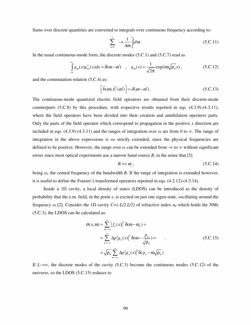
99
Sums over discrete quantities are converted to integrals over continuous frequency according to:
1 0
1
n
d∞∞
=
→ ω∆ω . (5.C.11)
In the usual continuous-mode form, the discrete modes (5.C.1) and (5.C.7) read as
( ) ( ) ( )g x g x dx∞
∗′ω ω
−∞
′= δ ω − ω , 0
1( ) exp( )
2g x i xω = ω ρ
π, (5.C.12)
and the commutation relation (5.C.4) as:
†ˆ ˆ( ), ( ) ( )b bω ω δ ω ω ′ ′= − . (5.C.13)
The continuous-mode quantized electric field operators are obtained from their discrete-mode
counterparts (5.C.8) by this procedure, with respective results reported in eqs. (4.3.9)-(4.3.11),
where the field operators have been divided into their creation and annihilation operators parts.
Only the parts of the field operator which correspond to propagation in the positive x direction are
included in eqs. (4.3.9)-(4.3.11) and the ranges of integration over are from 0 to . The range of
integration in the above expressions is so strictly extended, since the physical frequencies are
defined to be positive. However, the range over can be extended from - to without significant
errors since most optical experiments use a narrow band source B, in the sense that [5]
cB ω<< , (5.C.14)
being c the central frequency of the bandwidth B. If the range of integration is extended however,
it is useful to define the Fourier’s transformed operators reported in eqs. (4.2.12)-(4.3.14).
Inside a 1D cavity, a local density of states (LDOS) can be introduced as the density of
probability that the e.m. field, in the point x, is excited on just one eigen-state, oscillating around the
frequency [2]. Consider the 1D cavity C=(-L/2,L/2) of refractive index n0 which holds the NMs
(5.C.3), the LDOS can be calculated as:
2
2
0
20 0
( , ) ( ) ( )
( ) ( )
( ) ( )
n nn
nn
n
n nn
x f x
pp g x
p g x p
∞
=−∞
∞
=−∞
∞
=−∞
σ ω = δ ω − ω =
= ∆ δ ω− =ρ
= ρ ∆ δ − ω ρ
. (5.C.15)
If L, the discrete modes of the cavity (5.C.3) become the continuous modes (5.C.12) of the
universe, so the LDOS (5.C.15) reduces to

100
2( )0 0
2 00
( , ) ( ) ( )
( ) ( )2
locpx dp g x p
g x
∞
−∞
ω
σ ω = ρ δ − ω ρ =
ρ= ρ = σ ω =
π
. (5.C.16)
If the field operator ˆ ( )xωφ [eq. (4.3.12)] lies on a quantum state 0ψ , characterized by an
expectation value ˆ ( )H ω for the Hamiltonian operator [eqs. (4.3.40) and (4.3.39)], then the auto-
correlation of the e.m. field
0†0 0 2
0 0
ˆ ˆ ˆ( , , ) ( ) ( ) ( ) ( ) ( )F x x x x H g x g xn
∗ω ω ω ω
ρ′ ′ ′ω ψ φ φ ψ = π ω
ε (5.C.17)
is so linked with the LDOS (5.C.16):
( ) 20 0
1 ( , , )( , )
ˆ ( )loc F x x
x nH
ωσ ω = επ ω
. (5.C.18)
This link has been obtained in a homogeneous cavity and an extension of eq. (5.C.18) is used, with
the weight given by the value of the local index of refraction, in the case of inhomogeneous cavities
like Photonic Crystals (PC), in which a refractive index assumes different constant values in aligned
limited regions.
References.
[1] A. A. Asatryan, K. Busch, R. C. McPhedran, L. C. Botten, C. Martijn de Sterke, and N. A.
Nicorovici, Phys. Rev. E 63, 046612 (2001); D. Felbacq and R. Smaali, Phys. Rev. B 67, 085105
(2003).
[2] E. N. Economou, Green’s Functions in Quantum Physics (Springer-Verlag, Berlin, 1983).
[3] S. John, Phys. Rev. Lett. 53, 2169 (1984); S. John, Phys. Rev. Lett. 58, 2486 (1987); E.
Yablonovitch, Phys. Rev. Lett. 58, 2059 (1987); E. Yablonovitch and T. J. Gmitter, Phys. Rev. Lett.
63, 1950 (1989).
[4] J. Maddox, Nature (London) 348, 481 (1990); E. Yablonovitch and K.M. Lenny, Nature
(London) 351, 278, (1991); J. D. Joannopoulos, P. R. Villeneuve, and S. H. Fan, Nature (London)
386, 143 (1997).
[5] J. D. Joannopoulos, Photonic Crystals: Molding the Flow of Light (Princeton University Press,
Princeton, New York, 1995); K. Sakoda, Optical properties of photonic crystals (Springer Verlag,
Berlin, 2001); K. Inoue and K. Ohtaka, Photonic Crystals: Physics, Fabrication, and Applications
(Springer-Verlag, Berlin, 2004).

101
[6] G. D’Aguanno, M. Centini, M. Scalora, C. Sibilia, Y. Dumeige, P. Vidakovic, J. A. Levenson,
M. J. Bloemer, C. M. Bowden, J. W. Haus, and M. Bertolotti, Phys. Rev. E 64, 016609 (2001).
[7] J. M. Bendickson, J. P Dowling, and M. Scalora, Phys. Rev. E 53, 4107 (1996).
[8] G. D’Aguanno, N. Mattiucci, M. Scalora, M. J. Bloemer and A. M. Zheltikov, Phys. Rev. E. 70,
016612 (2004).
[9] K. C. Ho, P. T. Leung, Alec Maassen van den Brink and K. Young, Phys. Rev. E 58, 2965
(1998).
[10] P. T. Leung, S. Y. Liu, and K. Young, Phys. Rev. A 49, 3057 (1994); P. T. Leung, S. S. Tong,
and K. Young, J. Phys. A 30, 2139 (1997); P. T. Leung, S. S. Tong, and K. Young, J. Phys. A 30,
2153 (1997); E. S. C. Ching, P. T. Leung, A. Maassen van der Brink, W. M. Suen, S. S. Tong, and
K. Young, Rev. Mod. Phys. 70, 1545 (1998).
[11] S. C. Ching, H. M. Lai, and K. Young, J. Opt. Soc. Am. B 4, 1995 (1987); 4, 2004 (1987).
[12] S. Severini, A. Settimi, C. Sibilia, M. Bertolotti, M. Centini, A. Napoli, N. Messina, Quantum
counter-propagation in open cavities via Quasi Normal Modes approach, submitted to Journal of
Laser Physics (2005).
[13] A. Settimi, S. Severini, C. Sibilia, M. Bertolotti, M. Centini, A. Napoli, N. Messina, Phys. Rev.
E 71, 066606 (2005).
[14] S. Severini, A. Settimi, C. Sibilia, M. Bertolotti, A. Napoli, A. Messina, Quasi Normal
Frequencies in open cavities: an application to Photonic Crystals, in press on Acta Phys. Hung. B
(2006).
[15] A. Settimi, S. Severini, N. Mattiucci, C. Sibilia, M. Centini, G. D’Aguanno, M. Bertolotti, M.
Scalora, M. Bloemer, C. M. Bowden, Phys. Rev. E, 68, 026614 (2003).
[16] S. Severini, A. Settimi, C. Sibilia, M. Bertolotti, A. Napoli, A. Messina, Phys. Rev. E, 70
056614 (2004).
[17] J. J. Sakurai, Advanced Quantum Mechanics (Addison-Wesley, New York, 1995); S.
Weinberg, The Quantum Theory of Fields (Cambridge University Press, New York, 1996).
[18] K.J. Blow, R. Loudon, S. J.D. Phoenix, T.J. Shepherd, Phys. Rev. A 42, 4102 (1990).
[19] J. D. Jackson, Classical Electrodynamics (John Wiley, New York, 1975).
[20] A. A. Abrikosov, L. P. Gor’kov and I. E. Dzyaloshinski, Methods of Quantum Field Theory in
Statistical Physics (Dover, New York, 1975); P. T. Leung, A. Maassen van den Brink and K.
Young, Frontiers in Quantum Physics, Proceedings of the International Conference, edited by S. C.
Lim, R. Abd-Shukor and K. H. Kwek (Springer-Verlag, Singapore, 1998).
[21] M. Centini, G. D’Aguanno, M. Scalora, M. J. Bloemer, C. M. Bowden, C. Sibilia, N.
Mattiucci, and M. Bertolotti, Phys. Rev. E 67 036617 (2003).
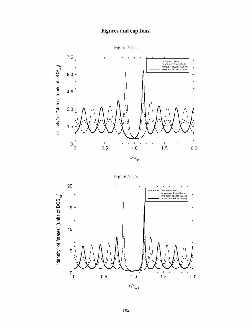
102
Figures and captions.
Figure 5.1.a.
Figure 5.1.b.
0
5
10
15
20
0 0.5 1.0 1.5 2.0
one laser-beamor vacuum fluctuationstwo laser-beams (∆ϕ=0)two-laser-beams (∆ϕ=π)
ω/ωref
"den
sity
" of
"st
ates
" (u
nits
of D
OS
ref)
0
1.5
3.0
4.5
6.0
7.5
0 0.5 1.0 1.5 2.0
one laser-beamor vacuum fluctuationstwo laser-beams (∆ϕ=0)two laser-beams (∆ϕ=π)
ω/ωref
"den
sity
" of
"st
ates
" (u
nits
of D
OS
ref)
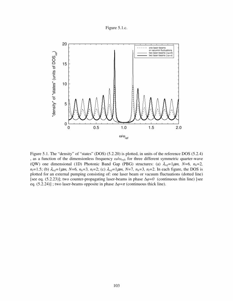
103
Figure 5.1.c.
Figure 5.1. The “density” of “states” (DOS) (5.2.20) is plotted, in units of the reference DOS (5.2.4), as a function of the dimensionless frequency /ref, for three different symmetric quarter-wave (QW) one dimensional (1D) Photonic Band Gap (PBG) structures: (a) λref=1µm, N=6, nh=2, nl=1.5; (b) λref=1µm, N=6, nh=3, nl=2; (c) λref=1µm, N=7, nh=3, nl=2. In each figure, the DOS is plotted for an external pumping consisting of: one laser beam or vacuum fluctuations (dotted line) [see eq. (5.2.23)]; two counter-propagating laser-beams in phase =0 (continuous thin line) [see eq. (5.2.24)] ; two laser-beams opposite in phase = (continuous thick line).
0
5
10
15
20
0 0.5 1.0 1.5 2.0
one laser-beamsor vacumm fluctuationstwo laser-beams (∆ϕ=0)two laser-beams (∆ϕ=π)
ω/ωref
"den
sity
" of
"st
ates
" (u
nits
of D
OS
ref)
104
Third Part:
QNM’s approach for emission processes in open cavities.

105
Chapter 6
Spontaneous Emission and coherent control of Stimulated Emission
inside one dimensional Photonic Crystals.
(Weak Coupling regime)
1. Introduction.
The behaviour of small systems (few degrees of freedom) coupled to dissipative reservoirs
represents a central theme in many physical contexts. In quantum optics, and in its simplest form,
the problem consists of a two-level excited atom decaying in open space to its ground state through
an allowed electric dipole transition; in this condition, the emitted radiation propagates away never
coming back to the atom. This is a prototype of irreversible decay of a prepared state, as well as a
classical manifestation of the quantization of the e.m. field [2].
Spontaneous or stimulated emission is a fundamental process resulting from the interaction between
radiation and matter. It depends not only on the properties of the excited atomic system but also on
the nature of the environment to which the system is optically coupled [2][3]. It is possible to
control the rate of spontaneous or stimulated emission from an excited atom by altering the photon
density of states (DOS) near the resonant frequency, i.e. by modifying the accessible states into
which the excited atom can radiate. If the photon DOS in the vicinity of the frequency of interest is
less than that of the free space, the atomic decay will be retarded, if it is greater it will be
accelerated [4],[5]; this link with the DOS has been put well into evidence in ref. [6].
An important and intriguing situation arose when it was realized that it is possible to create
environments in which the spectrum of the e.m. field exhibits gaps in frequency. In other words, no
radiation over some extended range of frequency can propagate in that environment; simply stated,
an excited atom whose transition frequency falls in the range of that gap should at first sight never
decay. The structures exhibiting such frequency gaps are referred to as photonic crystals (PC) or
even photonic band gap (PBG) structures [3]-[5]; in the wake of theoretical promulgation of PBGs,
concern has turned to the question of the behaviour of the atomic decay rate in such structures [10].

106
The photon DOS is the fundamental feature that determines the behaviour of the system ‘atom-
field’ and characterizes the various types of environments. The form and analytical properties of the
DOS dictate the type of the approximations permissible in formulating the equations governing the
time evolution of the system. When the photon DOS is a smooth function of frequency over the
spectral range of atomic transition, the rate of spontaneous and stimulated emission is described by
the Fermi’s golden rule. A substantial modification in the DOS can be effected by means of PBG
structures. Petrov et al [11] have reported some modifications of the emission processes of dye
molecules embedded in a three-dimensional solid-state PBG exhibiting a stop band in the visible
range; the results are interpreted in terms of a redistribution of photon DOS in the structure [12].
Ho et al. in ref. [2] already made an essential first step towards the application of the Quasi
Normal Mode’s (QNM’s) approach
[1] to quantum electrodynamics phenomema in a one side open and homogeneous cavity. In ref. [2],
the Feynman’s propagator inside the cavity is expressed in terms of QNMs, labeled by a discrete
index rather than a continuous momentum.
In ref. [8], the second quantization scheme based on the QNM’s approach has been extended to
double side open and inhomogeneous cavities [6], excited by vacuum fluctuations of the universe.
Although a full analysis of the spontaneous emission should be performed in three dimensional
geometries, ref. [8] puts into evidence that the QNM’s approach, limited to 1D-PBG structures, is
consistent with results already known in literature [4]-[19].
Using numerical methods, Centini et al. in ref. [5] have studied the propagation of counter-
propagating pulses in finite 1D-PBG structures. Linear interference and localization effects are
shown to combine to either enhancement or suppression of stimulated emission processes,
depending on the initial phase difference between the input pulses.
The main object of this chapter is to give a fully quantum treatment for the dynamics of an atom
inside a 1D-PBG structure, coupled with two counter-propagating laser-beams, by using the QNM’s
approach [10], i.e. treating the problem in the framework of open systems. The e.m. field is
quantized in terms of the QNMs inside the 1D-PBG and the atom is modelled as a two levels
system. In the electric dipole approximation, the atom is assumed to be weakly coupled to just one
of the QNMs. As a result, the decay-time depends from the position of the dipole inside the
structure, and can be controlled by the phase-difference of the two laser-beams. Such a system is
relevant for a single-atom, phase-sensitive, optical memory device on atomic scale.
The chapter is organized as follows. In section 2, the emission power of an atom is calculated inside
an open cavity, and a sensitivity function is defined for the atom-e.m. field coupling. In section 3,
the spontaneous emission processes are described inside a symmetric quarter wave (QW) 1D-PBG

107
structure. In section 4, the coherent control of the stimulated emission is discussed inside the same
1D-PBG. In section 5, the decay-times of the atom are compared with the dwell-times of the e.m.
radiation inside the structure [22]-[24]. Conclusions and discussion are given in section 6. In
appendix, if a dipole (a two-level system) is coupled with the Normal Modes (NMs) of universe, the
physical link between the emission power of the two-level system and the DOS for NMs [2] is
examined closely. This appendix is viewed as a key passage in order to pave a reasonable way of
generalization; if the dipole is coupled with the QNMs inside an open cavity, this kind of link is
retained to hold again between the emission power of the two-level system and the DOS for QNMs.
2. Atomic emission power inside open cavities.
In order to discuss the emission processes of an atom inside an open cavity excited by two
counter-propagating field pumps, let consider the atom as a two-level system and the e.m. field in
the cavity as a superposition of Quasi Normal Modes (QNMs). The cavity C=[0,d] is filled with a
medium of refractive index n(x). The dipole approximation [2] is assumed, so the two-level system
acts as an electrical dipole of length l, placed in a point x, which oscillates orthogonally to the x-
direction. At initial time t=0, the dipole is prepared in the excited state 0t
ψ=
= + , corresponding
to the higher energy, and its operator of momentum P is characterized by an expectation value
0ˆ ˆ
tP P
== + + . The dipole bandwidth is so narrow, if compared with QNM’s spectrum [2], that
the dipole is assumed to be (weakly) coupled with just one of the QNMs, being excited with a local
density of probability (loc)(x,) which corresponds to the local “density” of “states” (LDOS) for
QNMs, [Chapter 5].
At time t>0 , when the dipole is evolved in a superposition state ( )tψ [2], the time average for the
expectation value of e.m. power
tW , supplied by the dipole inside the open cavity, is inversely
proportional to the relative dielectric constant n2(x) and is directly linked to the QNM’s LDOS [see
Appendix D]
( )22 ( )
2 00
/ 2 ˆ ( , )( )
loc
ttW P l x
n xπ ω σ ω
ε == − , (6.2.1)
where 0 is the dielectric constant in vacuum.
If the cavity extends to the whole universe, then the e.m. field is reduced to a continuum of Normal
Modes (NMs); the refractive index becomes uniform, i.e. n(x)=n0, as well as the DOS for NMs, i.e.
( )0( , ) ( ) / 2loc
ref refxσ ω σ ω ρ π= = , being 0=(n0/c)2 and c the speed of the light in vacuum [Appendix

108
C]. The expectation value of the e.m. power (6.2.1), supplied by the dipole free in the universe,
reduces to:
( ) ( )2 202 2
2 20 00 0 0 0
/ 2 ˆ ˆ( )4reft tt
W P l P ln n
ρπ ω σ ω ωε ε= =
= − = − . (6.2.2)
If the two counter-propagating field pumps are filtered at frequency Ren, just the nth
QNM is excited and not the other QNMs, because the nth QNM oscillates at frequency Ren
within a narrow range 2|Imωn|<<|Reωn| , so distant enough from the other QNMs [2]. The e.m.
power n
tW , supplied by the dipole to the nth QNM,
( )22 ( )
2 00
/ 2 ˆ ( , )( )
locn ntt
W P l xn x
π ω σ ωε =
= − , (6.2.3)
is proportional to the local density of probability (LDOP) for the nth QNM [here, eq. (5.2.9) is
suitably reported]
2( ) 1
( , ) ( ) ( ) ( )locn n n
n
x x F xI
σ ω σ ω ρ= , (6.2.4)
which is directly linked to the (integral) density of probability (DOP) n() for the nth QNM. In eq.
(6.2.4), (x)=[n(x)/c]2, In denotes the usual overlapping integral and ( ) ( ) 2 n nf fn n nF x f x= ω
the normalized QNM’s function, being n nf f the QNM’s norm.
In order to discuss processes of spontaneous emission, the two field pumps describe vacuum
fluctuations in the universe, lying on the ground state of e.m fields [2]. The DOP for the nth QNM,
specified for vacuum fluctuations, is expressed as [eq. (5.2.12)]:
2
( )2 2
Im( )
2 ( Re ) Imn nA
n nn n
IdK
ωσ ω
π ω ω ω=
− +. (6.2.5)
The normalization constant nK can be obtained by the following condition:
Re Im
( )
Re Im
1( )
n n
n n
An d
d
ω ω
ω ω
σ ω ω+
−
= . (6.2.6)
In order to discuss processes of stimulated emission, the two field pumps describe two laser-beams
in the universe, lying on a coherent state of e.m. fields [2]. When the open cavity presents a
refractive index n(x) which satisfies the symmetry properties n(d/2−x)=n(d/2+x), the DOP for the
nth QNM, specified for the two laser-beams, is simplified as:
( ) ( )( ) ( )[1 ( 1) cos ]B A nn nσ ω σ ω ϕ= + − . (6.2.7)
As from eq. (6.2.7), the DOP for the nth QNM can be controlled by the phase-difference of the
two external laser-beams.
109
2. 1. Sensitivity function of dipole-e.m. field coupling.
Let define the sensitivity function S(x0, ) of a dipole-cavity coupling as the ratio between the
e.m. power (6.2.1) supplied by a dipole embedded inside an open cavity and the e.m. power (6.2.2)
supplied by the same dipole free in the universe:
0( , ) t
reft
WS x
Wω . (6.2.8)
Inserting eqs. (6.2.1) and (6.2.2) in eq. (6.2.8), it results that:
( )
0 2
0
( , )( )
( , )( )
loc
ref
x
S xn xn
σ ωσ ω
ω =
. (6.2.9)
If the relative dielectric constant is inhomogeneous, i.e. 2 20 ( )n n x→ , the LDOS is modified, i.e.
( )( ) ( , )locref xσ ω σ ω→ ; the sensitivity function S(x, ) can be expressed as the per-cent variation of
the LDOS, ( ) ( , ) ( )locrefxσ ω σ ω in units of the per-cent variation of the relative dielectric constant
2 20( )n x n . The meaning of the sensitivity function is ensued: eq. (6.2.9) provides a physical tool to
discuss the emission processes of a dipole excited inside a cavity with respect to the case of the
same dipole free in the universe.
If the sensitivity function Sn(x, ) of the dipole-nth QNM coupling, i.e.
2 ( )
0
0
( , )( , )
( ) ( )
locn
nref
n xS x
n xσ ωω
σ ω
=
, (6.2.10)
is developed inserting the LDOS of the nth QNM (6.2.4), it follows that (reminding (x)=[n(x)/c]2
and 0=(n0/c)2):
2
0
( ) ( )( , )
( )n n
nn ref
F xS x
Iσ ωω ρσ ω
= . (6.2.11)
If the dipole inside the open cavity (point x) is coupled to the nth QNM (frequency Ren), then
the sensitivity function Sn(x,) is linked both to the normalized intensity 2
nF of the nth QNM, in the
point x, and to the DOP n for the nth QNM, in the frequency Ren. So, the weak coupling of a
dipole to one QNM responds to the Fermi’s golden rule [2].
110
3. Spontaneous emission inside a symmetric QW 1D-PBG.
In this section, the QNM’s approach is applied to discuss about atomic spontaneous emission
processes inside a symmetric quarter wave (QW) one dimensional (1D) Photonic Band Gap
structure; this discussion, here reported, is revised respect the one reported in ref. [8] Let start with
the spontaneous emission of an atom [denoted as process A], inside an open cavity at a point x,
which is induced by vacuum fluctuations, oscillating outside the cavity at a frequency ω . The
conservative limit [2] is the unique case in which a single QNM can dominate, for the limit of
narrow resonances |Imωn|<<|Reωn|, and vacuum fluctuations can be coupled just to one QNM, i.e.
Ren. The sensitivity function (6.2.11) for the dipole-nth QNM coupling, in spontaneous
emission, can be calculated in terms of the DOP (6.2.5) for the nth QNM, due to vacuum
fluctuations:
2 ( )( )
0
20 2 2
( ) ( )( , )
( )
Im ( ) ( )
( Re ) Im
AnA n
nn ref
nn n n
n n
F xS x
I
K d I F x
σ ωω ρσ ω
ωρ
ω ω ω
= =
= ⋅ ⋅− +
. (6.3.1)
As an example, let consider a symmetric QW 1D-PBG structure with λref=1µm as reference
wavelength, N=6 periods, consisting of two layers with refractive indices nh=3 and nl=2 and
lengths h=λref/4nh and l=λref/4nl. The terminal layers of the 1D-PBG are characterized by the
parameters nh and h=λref/4nh and the length of the structure is d=N(h+l)+h. In the conservative
limit, a dipole can be coupled to just one of the 2N+1 QNMs in the [0, 2ref) range, which can be
enumerated, excluding =2ref, as 0,nn = , ]2,0[ Nn ∈ [6].
It is necessary to report some considerations about the QNM’s functions and the QNM’s DOS of a
symmetric QW 1D-PBG [8], useful to discuss the spontaneous emission processes inside the
structure. So, the highest e.m. field for the 1D-PBG structure with N periods is found inside a
central layer with low refractive index, and can be approximated to the absolute maximum of the
QNM 1N + , with frequency close to the high-frequency band-edge. If the 1D-PBG is composed
by an even (odd) number of periods, i.e. N=2,4,… (N=3,5…), the central layer, i.e. the (N+1)th one,
is characterized by the high (low) refractive index nh (nl); so the absolute maximum of the QNM
1N + is found in the adjacent layers (central layer), i.e. the (N-1)th and (N+2)th ones (just the
(N+1)th one). In the centre x=d/2 of the structure, the QNM’s functions present a maximum for
even values of n and are null for odd values of n and, on the two terminal surfaces x=0 and x=d,
all the QNM’s functions present the same value (in modulus). The photonic band-gap is in a region
111
/ref=(0.8249, 1.175); the DOS for QNMs is suppressed in the gap and is enhanced at the band-
edge resonances.
In the figures 6.2, the spontaneous emission processes are described in terms of the sensitivity
functions ( )AnS , plotted as functions of the dimensionless space x/d and the dimensionless
frequency /ref . In (a) is depicted the sensitivity function ( )1
ANS − , for the coupling dipole- 1N −
(where the real part of the QNM’s frequency is close to the first transmission peak before the low-
frequency band-edge); in (b), the sensitivity function ( )ANS , for the coupling dipole- N
(corresponding to the low-frequency band-edge, being I band-edge/ref = 0.8249); in (c) is depicted
the sensitivity function ( )1
ANS + , for the coupling dipole- 1N + (where the real part of the QNM’s
frequency is close to the high-frequency band-edge, being II band-edge/ref = 1.175) and, in (d), the
sensitivity function ( )2
ANS + , for the coupling dipole- 2N + (corresponding to the first transmission
peak after the high-frequency band-edge). The sensitivity functions ( )ANS and ( )
1A
NS + , with frequencies
close to the two band edges, stand out respect to ( )1
ANS − and ( )
2A
NS + corresponding to the two adjacent
transmission peaks, because, next to the two band-edges resonances, the DOS for QNMs is
enhanced and the QNM’s functions present the most large intensities inside the 1D-PBG structure.
Moreover, the sensitivity functions ( )AnS is centred around the frequency Ren of the nth QNM and,
like the QNM’s function Fn(x), has n minima along the x-direction. Let note that the QNM’s
approach uses a realistic model for the 1D-PBG, as a finite structure with discontinuities in the
refractive index, so this approach improves the results of ref. [4], obtained by the Kronig-Penney
model.
In the figures 6.3, the sensitivity functions ( )ANS and ( )
1A
NS + , with frequencies close to the two band-
edges, and ( )1
ANS − , ( )
2A
NS + , corresponding to the two adjacent transmission peaks, are plotted, as
functions of the dimensionless frequency /ref, when: (a) the dipole is embedded inside the 4th
period of the 1D-PBG structure, and it is exactly in the centre x=(d/2)+(/2) of the low-index layer,
being =h+l. The sensitivity functions ( )AnS , ]2,0[ Nn ∈ are depicted, when: (b) the dipole is
embedded inside the 4th period of the 1D-PBG structure, and it is exactly in the centre x=d/2 of the
high-index layer, being also the centre of the 1D-PBG; (c) the dipole lies on one of the two terminal
surfaces x=0 and x=d of the 1D-PBG. In all figs 6.3.a-c, the sensitivity function is strongly
suppressed over the band gap /ref=(0.8249, 1.175), since the QNM’s DOS is there suppressed.
When the dipole is embedded inside the 4th period of the structure, if it is in the centre
x=(d/2)+(/2) of the low index layer (fig. 6.3.a.): the sensitivity function ( )1
ANS + , corresponding to the

112
high-frequency band-edge, is enhanced, because, in x=(d/2)+(/2), the eigen-function FN+1(x) of the
QNM 1N + assumes the absolute maximum [see fig. 6.2.]; moreover, the sensitivity function
( )ANS , corresponding to the low-frequency band-edge, is almost suppressed, because, even if the
QNM’s DOS is large, the QNM’s function FN(x) is almost null where the QNM’s intensity FN+1(x)
is maximum [8]. For the 1D-PBG with parameters above reported, i.e. λref=1µm, N=6, nh=3 and
nl=2, the peak of sensitivity function ( )1
ANS + assumes the absolute maximum Smax=18.55 (as
previously stated in some considerations); in x=(d/2)+(/2), the peak of the sensitivity function ( )ANS , in units of Smax is 0.006, the peak of the sensitivity function ( )
1A
NS − , in units of Smax, is 0.1507
and the ratio between the peak of the sensitivity function ( )2
ANS + and the peak of the sensitivity
function ( )1
ANS − is 0.4966.
When the dipole is embedded inside the 4th period of the structure (N=6 periods), if it is in the
centre of the high-index layer (i.e. x=d/2) [see fig. 6.1.], the sensitivity functions in the low and
high frequency band-edges exchange their physical behaviour; the sensitivity function ( )ANS , in the
low-frequency band-edge (the Nth one, an even peak) is enhanced, and the sensitivity function ( )1
ANS + ,
in the high-frequency band-edge (the (N+1)th one, an odd peak), is suppressed (fig. 6.3.b.). In fact,
in the centre of the structure, the dipole can be coupled just to one of the QNMs n with an even n,
because, in x=d/2, the QNM’s function Fn(x) has a maximum for even values of n and is null for
odd values of n [see fig. 6.2.] [8]. For the 1D-PBG with parameters above reported, in x=d/2, the
peak of ( )ANS , in units of Smax is 0.6905; instead, the ratio between the peak of the ( )
2A
NS − and the peak
of ( )ANS is 0.3565.
When the dipole lies on the terminal surfaces x=0 and x=d of the structure (fig. 6.3.c.): the dipole
can be coupled to any of the QNMs n (in fact, any of the QNM’s functions Fn(x) is not null on
x=0 and x=d); moreover, the peaks of the sensitivity functions ( )ANS and ( )
1A
NS + , present values
similar to the peaks of the sensitivity functions ( )AnS , as it could be intuitively suggested (all the
QNM’s functions Fn(x) have the same values on x=0 and x=d). For the 1D-PBG considered, in x=0
and x=d, the ( ), 1
An N NS = + peak in units of Smax is 0.2239; instead, the peak ratio ( ) ( )
1, 2 , 1/A An N N n N NS S= − + = + is
1.0265.
The QNM’s approach to discuss the spontaneous emission processes of a dipole inside a 1D-PBG
presents the advantage to develop a general quantum treatment. This approach agrees with the
113
theoretical results of ref. [18], which consider only a classical model. Moreover, the approach
confirms the results of ref. [19], which is only a numerical investigation.
4. Coherent control of stimulated emission inside a symmetric QW 1D-PBG.
In the following sections, the QNM’s approach is applied to discuss how a coherent control of
the atomic stimulated emission processes inside a symmetric QW 1D-PBG can be effected by the
phase-difference of two counter-propagating laser-beams [10]; such a system is relevant for a
single-atom, phase-sensitive, optical memory device on atomic scale. Let start with the stimulated
emission of an atom [denoted as process B], inside a symmetric cavity [refractive index n(x) such
that n(d/2−x)=n(d/2+x)], which is induced by two counter-propagating laser-beams (phase-
difference ). As stated in advance, the conservative limit is the unique case in which a single
QNM can dominate, for the limit of narrow resonances |Imωn|<<|Reωn|, and the two laser-beams
can be coupled just to one QNM, i.e. Ren. The sensitivity function (6.2.11) for the dipole-nth
QNM coupling, in stimulated emission, can be calculated in terms of the DOP (6.2.7) for the nth
QNM, due to the two laser-beams:
2 ( )( )
0
2 ( )( )
0
( ) ( )( , )
( )
( ) ( )[1 ( 1) cos ] ( , )[1 ( 1) cos ]
( )
BnB n
nn ref
A nn A nn
nn ref
F xS x
I
F xS x
I
σ ωω ρσ ω
σ ω ϕρ ω ϕσ ω
= =
+ − ∆= = + − ∆
. (6.4.1)
As from (6.4.1), the sensitivity function of the dipole-nth QNM coupling, for stimulated emission
inside an open cavity, depends on the phase-difference of two external counter-propagating laser-
beams. If the dipole is embedded in a point of the cavity in which the normalized intensity of the nth
QNM is almost null, all the emission processes are inhibited. Otherwise, if the dipole is in a point of
the cavity in which the nth QNM intensity is not null, it can be coupled to one of the QNMs with an
even n, when the two laser-beams are in phase =0, while it can be coupled to one of the QNMs
with an odd n, when the two laser-beams are opposite in phase =.
As an example, let consider the symmetric QW 1D-PBG structure with parameters above reported,
i.e. λref=1µm, N=6, nh=3 and nl=2. As stated in advance, in the conservative limit, a dipole can be
coupled to just one of the 2N+1 QNMs in the [0, 2ref) range, which can be enumerated, excluding
=2ref, as 0,nn = , ]2,0[ Nn ∈ . In figure 6.4, the stimulated emission processes are described
by the sensitivity functions ( )BnS of (6.4.1), plotted as functions of the dimensionless space x/d and
the dimensionless frequency /ref . The sensitivity function ( )1
ANS + for the coupling dipole- 1N + (

114
corresponding to the high-frequency band-edge) is depicted, when the two laser beams are nearly in
phase, (a) =/4, or nearly opposite in phase, (b) =3/4. It is clear that the dipole, inside the
1D-PBG structure, can be actually coupled with the QNM 1N + , in the high-frequency band-edge
(i.e. the (N+1)th one, an odd peak), only when the two laser-beams tend to be opposite in phase (i.e.
). The amplification factor of the stimulated emission respect to the spontaneous emission is
identified as 1+(-1)ncos, which assumes the values 0.2929 in fig 6.4.a and 1.7071 in fig 6.4.b.
5. Decay-times in units of dwell-times.
The spontaneous emission process of a dipole lying on a terminal surface (x=0) of an open
cavity is characterized by a decay-time
( )( )
1(0)
(0)A
n An
τω
=∆
, (6.5.1)
being ( ) (0)Anω∆ the bandwidth of the sensitivity function ( ) (0, )A
nS ω at half height [i.e.
( ) (0, Re ) / 2An nS ω ω= ]. After some algebra, reminding 2
0(0) Imn nF ω ρ= , it results that:
( ) 1(0)
2 ImA
nn
τω
= . (6.5.2)
It is clear that no emission occurs [ ( ) (0)Anτ → ∞ ] when the cavity is closed [|Imωn|0].
The spontaneous emission process of a dipole in a point x of the cavity is characterized by a decay-
time
( )( )
1( )
( )A
n An
xx
τω
=∆
, (6.5.3)
being ( ) ( )An xω∆ the bandwidth of the sensitivity function ( ) ( , )A
nS x ω at the half height of ( ) (0, )AnS ω .
After some algebra, it results that (see ref. [10]):
( )
2( )2
0
(0)1( )
4 ( )
AA n n
n
n
d Ix
F x
ττρ
⋅ ≅
. (6.5.4)
As from eq. (6.5.4), in case of spontaneous emission processes inside an open cavity, the decay-
time of the dipole-nth QNM coupling depends from the position of the dipole in the cavity.
If the cavity of length d is pumped by vacuum fluctuations, filtered at Ren, it is possible to
introduce the dwell-time [22][8] of vacuum fluctuations, linked to the DOP (6.2.5) for the nth QNM:
( ) ( )2 2
( ) ( )2 2
Im( ) ( )
2 ( Re ) Im 2 Imnn nA A n
n n nn n n
d I d IKt d K
ωδ ω σ ω
π ω ω ω π ω⋅ ⋅
⋅ = ≅− +
. (6.5.5)

115
The decay-time (6.5.2) of the dipole coupled with the nth QNM, when the dipole lies on a terminal
surface (x=0), is different from the dwell-time (6.5.5) of vacuum fluctuations at Ren; in fact, if
the dipole is on one surface of a symmetric QW 1D-PBG structure with parameters λref=1µm, N=6,
nh=3, nl=2 and it is excited by vacuum fluctuations filtered at one band-edge, i.e. I band-edge/ref
0.8249 or II band−edge/ref 1.175, then the decay-time is ( )0( 0) 33.30A
band edge xτ − = ≅ in units of 1/ref,
and the ratio between the decay-time and the dwell-time is ( ) ( )0( 0) 1.571A A
band edge band edgex tτ δ− −= ≅ .
The stimulated emission process of a dipole embedded in a point x of the open cavity is
characterized by a decay-time
( )( )
1( )
( )B
n Bn
xx
τω
=∆
, (6.5.6)
being ( ) ( )Bn xω∆ the bandwidth of the sensitivity function ( ) ( , )B
nS x ω at the half height of ( ) (0, )AnS ω .
After some algebra, it results that (ref. [10]):
( )
( ) ( )( )
1 ( 1) cos
AB n
n n
xx
ττϕ
≅+ − ∆
. (6.5.7)
All the bandwidths ( ) (0)Anω∆ , ( ) ( )A
n xω∆ and ( ) ( )Bn xω∆ are referred to the half length of ( ) (0, )A
nS ω ,
so the decay-times (6.5.2), (6.5.4) and (6.5.7) run from the same instant. As from eq. (6.5.7), in case
of stimulated emission inside an open cavity pumped by two counter-propagating laser-beams, the
decay-time of the dipole-nth QNM coupling in a point of the cavity can be controlled by the phase-
difference of the two laser-beams.
Figure 6.5 refers to an excited dipole, embedded inside a symmetric QW 1D-PBG structure with
parameters λref=1µm, N=6, nh=3, nl=2, pumped by two counter-propagating field pumps filtered at
low-frequency band-edge (fig. 6.5.a.) or at high-frequency band-edge (fig. 6.5.b.). The decay-time
τ, in units of the decay-time τref for spontaneous emission when the dipole lies on one terminal
surface (x=0) of the structure [eq.(6.5.2)], is plotted as a function of the dimensionless position x/d
of the dipole, being d the length of the 1D-PBG. Several cases are shown: the spontaneous emission
[see eq.(6.5.4)], when the two field pumps describe vacuum fluctuations (); and the
stimulated emission [see eq.(6.5.7)], when the two pumps describe two input laser-beams, nearly in
phase (− − −) or opposite of phase ( − ). So, in the low-frequency (high-frequency) band-edge,
all the emission processes are enhanced if the dipole is inside the layers with high (low) refractive
index; while, the stimulated emission can be inhibited increasing (reducing) the phase-difference of
the two laser-beams if the dipole is inside the layers with low (high) refractive index. In fact, next to
the low-frequency (high-frequency) band-edge, the DOS is minimum if the two laser-beams are
opposite of phase (in phase) [fig.5.1.b.]. Figure 6.5.a.bis. (fig. 6.5.b.bis.) is a magnification of fig.

116
6.5.a. (fig. 6.5.b.) for the decay-time when the dipole is in the 3th and 4th periods of the 1D-PBG. If
the dipole is centred into the structure, the decay-time is accelerated (tends to be highly retarded) in
the low-frequency (high-frequency) band-edge. In fact, in the centre of the structure, the QNM
corresponding to the low-frequency (high-frequency) band-edge is maximum (tends to zero) [as
stated in some considerations after eq. (6.3.1)].
If an open cavity of length d is pumped by two counter-propagating laser-beams tuned at the
frequency Ren (phase-difference ), it is possible to introduce the dwell-time of the two laser-
beams, linked to the DOS (6.2.7) for the nth QNM [10]:
( ) ( ) ( ) ( )[1 ( 1) cos ] [1 ( 1) cos ]B B A n A nn n n nt d d tδ σ σ ϕ δ ϕ⋅ = ⋅ + − ∆ = + − ∆ . (6.5.8)
The decay-time (6.5.7) for stimulated emission of the dipole, coupled with the nth QNM, and the
dwell-time (6.5.8) of the two laser-beams, tuned at the nth transmission resonance, are dual
functions; in fact, the stimulated emission is inhibited [ ( )0( )B
n xτ → ∞ ] when the two laser-beams are
reflected by the cavity [ ( ) 0Bntδ = ], and it is enhanced [ ( )
0( )Bn xτ is minimum] when the two laser-
beams “stand” in the cavity [ ( )Bntδ is maximum].
Figure. 6.6. refers to the excited dipole embedded inside the symmetric QW 1D-PBG of fig. 6.5.,
pumped by two counter-propagating laser-beams filtered at low-frequency band-edge (fig. 6.6.a.) or
at the high-frequency band-edge (fig. 6.6.b.). The decay-time for stimulated emission (), in
units of the decay-time for spontaneous emission [eq. (6.5.7)], is compared with the dwell-time (− −
−) for the two laser-beams, in units of the dwell-time for vacuum fluctuations [eq. (6.5.8)]. The
decay-time for stimulated emission and the dwell-time for the two laser-beams are compared on
different scales as functions of the phase-difference between the two laser-beams. In the low-
frequency (high-frequency) band-edge, the decay-time ratio is rising (slopes down) and so the
dwell-time ratio slopes down (is rising) when the phase-difference of the two laser-beams is
increasing from =0 to =; in fact, the decay-time [figs. 6.5.a. and 6.5.b.] tends to the
maximum (minimum) and the DOS [fig. 5.1.b.] tends to the minimum (maximum) when the laser-
beams are going opposite of phase. Then, in the low-frequency (high-frequency) band-edge, the
decay-time ratio tends to infinity and so the dwell-time ratio is null when the phase-difference of the
two laser-beams is = (=0); in fact, the dipole is not coupled to the QNM corresponding to
the low-frequency (high-frequency) band-edge when the two laser-beams are opposite in phase (in
phase) [as stated in some considerations after eq. (6.4.1)].
6. Discussion and conclusions.
117
Non-Hermitian Hamiltonians and the ensuing complex eigen-values figure prominently in
Siegman’s work on dissipative cavity quantum electro-dynamics (CQED) [4], elaborating the Fox
and Lee’s works [5], which consider eigen-value problems for complex symmetric operators.
However, refs. [4] and [5] deal with transverse modes in the semi-classical limit, only considering
(a) c-number fields with some effective quantum noise, and (b) the limit <<d, being the field
wavelength and d the length of the cavity.
The present chapter pertains to a different regime; several numerical simulations have pointed out
the physical link between the sensitivity function of an atom-e.m. field coupling and the density of
states (DOS) for Quasi Normal Modes (QNMs) inside an open cavity.
As main object, a fully quantum treatment is given for the dynamics of an atom inside a 1D-PBG
structure, coupled with two counter-propagating laser-beams, by using the QNM’s approach, i.e.
treating the problem in the framework of open systems. The e.m. field has been quantized in terms
of the QNMs inside the 1D-PBG and the atom has been modelled as a two levels system. In the
electric dipole approximation, the atom has been assumed to be weakly coupled to just one of the
QNMs. As a result, the decay-time depends from the position of the dipole inside the structure, and
can be controlled by the phase-difference of the two laser-beams. Such a system is relevant for a
single-atom, phase-sensitive, optical memory device on atomic scale.
Appendix D. Examining deeper the link of atomic emission power
with density of states (DOS).
Let consider, according to classical electro-dynamics [15], a dipole which is radiating an
e.m. field in the universe, and then let discuss, applying second quantization rules [2], the coupling
of a two-level system with normal modes (NMs) of the universe; the physical link between the
emission power of the dipole and the “density” of “states” (DOS) for NMs is examined deeper: in
fact, this link is not clearly discussed in literature. This proof is viewed as a key passage in order to
pave a reasonable way of generalization; if the two-levels system is coupled with the Quasi Normal
Modes (QNMs) inside an open cavity, this kind of link is retained to hold again between the
emission power of the dipole and the DOS for QNMs. Besides, the proof enables to solve some
self-contradictions in the expressions of the emission power which are reported in refs. [24] and [8].
D. 1. Current density producing an e.m. field in the universe.

118
Let refer to a Cartesian frame xyz. The universe is modelled as an infinite one dimensional
cavity, ( / 2, / 2) , x C L L L∈ = − → ∞ , which is filled with a linear, isotropic and homogeneous
dielectric, dissipative for an electrical conductibility , with a dielectric constant =0r and a
magnetic permeability =0r0. No charge distribution is present and a current distribution Jy(x,t),
which oscillates along the direction of the y-axis, produces an e.m. plane wave Ey(x,t) and Hz(x,t),
which is a transverse electric and magnetic field respect to the x-axis.
Under the monochromatic condition, the current density oscillates just at one frequency
1
( , ) [ ( , ) exp( ) . .]2y yJ x t J x i t c cω ω= − + , (6.D.1)
and so the e.m. field
1( , ) [ ( , ) exp( ) . .]
21
( , ) [ ( , ) exp( ) . .]2
y y
z z
E x t E x i t c c
H x t H x i t c c
ω ω
ω ω
= − +
= − +
, (6.D.2)
satisfies the equations [15]
22
0 02
0
( , ) ( , )
1( , )
x yy y
x yz
EE x i J x
xE
H xi x
ρ ω ω ωµ ω
ωωµ
∂+ = −
∂∂
=∂
, (6.D.3)
where 0=(n0/c)2, being 0 rn ε≅ the refractive index of the dielectric material and 0 01c µ ε= the
speed of the light in vacuum.
The Green’s function of the e.m. problem (6.D.3) is defined as the solution of the equation [15]
2
202 ( , , ) ( )xG G x x x x
xρ ω ω δ∂ ′ ′+ = − −
∂, (6.D.4)
where (x-x’) is the Dirac’s delta function and x, x’ stand for observation-point and the source-point
respectively. The Green’s function G(x,x’,) is named as the kernel of the e.m. problem (6.D.3)
because it allows to obtain the corresponding solution:
0( , ) ( , ) ( , , )y yE x i J x G x x dxω ωµ ω ω∞
−∞
′ ′ ′= . (6.D.5)
In universe, an energetic balance is settled between the current distribution and the e.m. plane
wave. In time domain, the e.m. power supplied by the current density Jy(x,t) to the e.m. field Ey(x,t)
is defined as [15]
1
( ) ( , ) ( , ) ( , )2 y yW t w x t dx J x t E x t dx
∞ ∞
−∞ −∞
= = − , (6.D.6)
so, in the period T=2/, the time average of the e.m. power (6.D.6) is calculated as:
119
2
2
1( )
T
T
W W t dtT −
= . (6.D.7)
Instead, in frequency domain, a complex power supplied by the current density ( , )yJ x ω to the e.m.
field ( , )yE x ω can be defined [15]
1( ) ( , ) ( , ) ( , )
2yyW w x dx J x E x dxω ω ω ω
∞ ∞∗
−∞ −∞
= = − , (6.D.8)
such that the time-average of the e.m. power (6.D.7) can be calculated as the real part of the
complex power (6.D.8):
Re[ ( )]W W ω= . (6.D.9)
D. 2. Electrical dipole.
Let consider an electrical dipole of length l and charge q(t)=(1/2) [q0exp(-it)+c.c.]. The
momentum of the dipole is p(t)=lq(t)=(1/2) [p0exp(-it)+c.c.], being p0=q0l. The intensity of the
electrical current which flows inside the dipole is defined as
( ) 1 2[ ( )exp( ) . .]I t dq dt I i t c cω ω= = − + , being 0( ) ( )I i p lω ω= − . If the dipole is placed in the x0
point and oscillates along the direction of the y-axes, then, in frequency domain, the density of the
current ( , )yJ x ω , such that ( , ) ( )yJ x dx Iω ω∞
−∞
= , is operatively defined as:
0 0 0( , ) ( ) ( ) ( ) ( )yJ x I x x i p l x xω ω δ ω δ= − = − − . (6.D.10)
It results that, the e.m. field produced by the dipole is obtained inserting eq. (6.D.10) in eq. (6.D.5)
20 0 0( , ) ( ) ( , , )yE x p l G x xω µ ω ω= , (6.D.11)
the complex power supplied by the dipole to the universe is obtained inserting eqs. (6.D.10) and
(6.D.11) in eq. (6.D.8)
2
30 00 0( ) ( , , )
2p
W i G x xl
µω ω ω = −
, (6.D.12)
and the time-average of the power supplied by the dipole is obtained inserting eq. (6.D.12) in eq.
(6.D.9):
2
30 00 0Im ( , , )
2p
W G x xl
µ ω ω =
. (6.D.13)
As from eq. (6.D.13), the time average of the power W supplied by the electrical dipole to the
universe depends on the resonance of the dipole and it is linked to the square modulus of the

120
momentum p0 and then to the position of the dipole x0 via the imaginary part of the universe
Green’s function G(x0, x0, ). It is easy to verify that the physical link (6.D.13) holds also for a
dipole inside an inhomogeneous cavity, if the Green’s function G(x, x’, ) is referred to a cavity
which is filled with a medium of refractive index n(x).
D. 3. Feynman’s propagator.
To solve for the kernel equation (6.D.4), let introduce the Fourier’s space-transform of the
Green’s function
1( , , ) ( , ) exp[ ( )]
2G x x G k ik x x dkω ω
π
∞
−∞
′ ′= − , (6.D.14)
and the Fourier’s representation of the Dirac’s delta function [14]:
1
( ) exp( )2
x ikx dkδπ
∞
−∞
= . (6.D.15)
If the Fourier’s space-transforms (6.D.14) and (6.D.15) are applied on equation (6.D.4), the space-
transformed Green’s function is obtained:
2 202 2
0
1 1( , ) ,
2G k k
kω ρ ω
ρ ωπ= ≠
−. (6.D.16)
However, there is an ambiguity; let put this expression into the Fourier’s transform (6.D.14) and try
to perform the integration over the variable k: the integrand presents the poles 0k ω ρ± = ± and
therefore the integration cannot be performed over the real axis for the poles k± .
To get around this ambiguity, let adopt the Feynman’s prescription [4]; the Green’s function is
replaced by a complex propagator: so, in the transformed space-domain
2 2 2 2
0 0
0 0 0
20
1 1 1 1( , )
2 2 ( )
1 1 1 1 ,
2 2( ) ( ) ( )
2 , ,
F kk i k i
ki k i k i
i i
ωρ ω ηπ π ω ρ η
π ω ρ η ω ρ η ω ρ η
η η η ω ρ η η +
∆ = =′− + − −
= − ∈
− − − + −
′ ′= + ∈
, (6.D.17)
and in the effective space domain
1( , , ) ( , ) exp[ ( )]
2FF x x k ik x x dkω ω
π
∞
−∞
′ ′∆ ∆ − . (6.D.18)
If the parameter tends to zero, the complex propagator reduces, in transformed space-domain, to
the Green’s function

121
0
( , ) lim ( , )FG k kη
ω ω→
∆ , (6.D.19)
and, in effective space domain, to the Feynman’s propagator which is not the simple Green’s
function:
0 0
0
1( , , ) lim ( , , ) lim ( , ) exp[ ( )]
2
1 1 ( , , ) ( , ) exp[ ( )] lim ( , ) exp[ ( )]
2 2
FF F
F
G x x x x k ik x x dk
G x x G k ik x x dk k ik x x dk
η η
η
ω ω ωπ
ω ω ωπ π
∞
→ →−∞
∞ ∞
→−∞ −∞
′ ′ ′∆ = ∆ − ≠
′ ′ ′≠ = − = ∆ −
.
(6.D.20)
The complex analysis [14] provides the following result
0
exp( )lim 2 ( )
ikxdk i x
k iηπ θ
η
∞
→−∞
− = −+ , (6.D.21)
being (x) the unit step function. To calculate the Feynman’s propagator (6.D.20), the result
(6.D.21) is used, after inserting eq. (6.D.17) into eq. (6.D.18):
0 00
( , , ) exp[ ( )] ( ) exp[ ( )] ( )2
F
iG x x i x x x x i x x x xω ω ρ θ ω ρ θ
ω ρ′ ′ ′ ′ ′= − − − − + − − − .(6.D.22)
The e.m. field inside the universe consists on a continuum of NMs:
0
1( ) exp( ) ,
2g x i xω ω ρ ω
π= ∈ . (6.D.23)
The DOS for NMs is defined as the density of probability that the e.m. field, excited inside the
universe, consists of one NM, tuned at the frequency , so the DOS for NMs is calculated as
[Appendix C]
2( )0 0( , ) ( ) 2 loc x g xωσ ω ρ ρ π= = . (6.D.24)
It results that, in frequency domain, the Feynman’s propagator (6.D.22) of the universe can be
expressed in terms of the NMs (6.D.23)
0
( , , ) ( ) ( ) ( ) ( ) ( ) ( )F
iG x x g x g x x x g x g x x xω ω ω ω
πω θ θω ρ
∗ ∗′ ′ ′ ′ ′ = − − + − , (6.D.25)
and it can be linked to the NM’s DOS (6.D.24)
( )0
1( , ) Im ( , , )loc
Fx G x xσ ω ρ ω ωπ
= − , (6.D.26)
being ( ) 1 2x xθ ′= . As from eq. (6.D.26), the DOS is linked to the imaginary part of the
Feynman’s propagator.
D. 4. Two-levels system.
122
Let quantize an atom as a two-levels system [2]. The atomic Hamiltonian 0H admits only
two eigen-values E- and E+> E- , corresponding to two eigen-states − and + , i.e.
0H E±± = ± . (6.D.27)
The atom is assumed to be coupled with the e.m. field in the universe, which is quantized as a
continuum of NMs. The total Hamiltonian H is the sum between the unperturbed Hamiltonian 0H
of the atom and the perturbation intH of the atom-e.m. field coupling, i.e.
0 intˆ ˆ ˆH H H= + . (6.D.28)
Let adopt the dipole approximation [2], so the atom acts as an electrical dipole of length l which is
placed in the x0 point and oscillates along the direction of the y-axes [see section D.2.]. To discuss
emission processes, at initial time t=0, the dipole is assumed to be in the unperturbed state +
corresponding to the higher energy E+, i.e.
0t
ψ=
= + , (6.D.29)
so, the momentum of the dipole is described by an observable P , which is characterized by the
expectation value:
0
ˆ ˆt
P P=
= + + . (6.D.30)
If the dipole is weakly coupled with the e.m. field of the universe, i.e. int 0ˆ ˆH H , at time t>0, the
state of the dipole ( )tψ can be represented as a linear superposition of the unperturbed states −
and + , i.e.[2]
1 2( ) ( ) ( )t c t c tψ = − + + . (6.D.31)
The Ehrenfest’s theorem can be applied under the dipole and weak-coupling approximations. So,
according to eq. (6.D.13), the time average for the expectation value of the e.m. power in the state
(6.D.31), supplied to one NM (frequency ) of the universe by the electrical dipole (length l, point
x0, initial momentum 0
ˆt
P=
), can be expressed in terms of the imaginary part of the Feynman’s
propagator, i.e.
( )230
0 00ˆ Im ( , , )
2 FttW P l G x x
µ ω ω=
= . (6.D.32)
As well as eq. (6.D.13) [see comments], eq. (6.D.32) holds also for a two-levels system inside a
inhomogeneous cavity, if the Feynman’s propagator GF(x, x’, ) satisfies the boundary conditions
of a cavity which is filled with a medium of refractive index n(x).
123
Recalling that ( )2 20 0 0 0 0n c nρ µ ε= = , the e.m. power (6.D.32) supplied by the electrical dipole to
one NM of the universe can be expressed in terms of the NM’s DOS (6.D.26), i.e.
( )22 ( )
02 00 0
/ 2 ˆ ( , )loc
ttW P l x
nπ ω σ ωε =
= − , (6.D.33)
and, inserting eq. (6.D.24), it results that the e.m. power (6.D.33) is uniform in the space:
( )20 2
2 00 0
ˆ 4
reftt
W P ln
ρω
ε == − . (6.D.34)
The physical link (6.D.34) holds also for QNMs inside an open cavity, if the local QNM’s DOS
satisfies the boundary conditions of a cavity filled with a medium of refractive index n0 [20].
Moreover, the physical link (6.D.34) can be generalized for QNMs inside an inhomogeneous cavity
of refractive index n(x),
( )22 ( )
02 00 0
/ 2 ˆ ( , )( )
loc
ttW P l x
n xπ ω σ ω
ε == − , (6.D.35)
if the QNMs oscillate at wavelengths so short that the refractive index of the cavity can be
considered as smooth [6]
( ) 4dn x
dxπλ
<< . (6.D.36)
References.
[1] J. J. Sakurai, Advanced Quantum Mechanics (Addison-Wesley, New York, 1995); S. Weinberg,
The Quantum Theory of Fields (Cambridge University Press, New York, 1996).
[2] E. M. Purcell, Phys. Rev. 69, 681 (1946); D. Kleppner, Phys. Rev. Lett. 47, 233 (1981).
[3] E. A. Hinds, Adv. At., Mol., Opt. Phys. 28, 237 (1991).
[4] M. Lewenstein, J. Zakrzewski, T. M. Mossberg, and J. Mostowski, J. Phys. B 21, L9 (1988); M.
Lewenstein, J. Zakrzewski, and T. M. Mossberg, Phys. Rev. A 38, 1075 (1988).
[5] S. Haroche, in New Trends in Atomic Physics, edited by G.Grynberg and R.Stora, Proceedings
of the Les Houches Summer School of Theoretical Physics, XXXVIII, 1982 (North-Holland,
Amsterdam, 1982), p.193.
[6] Z. Huang, C. Lei, D. G. Deppe, C. C. Lin, C. J. Pinzone, and R. D. Dupuis, Appl. Phys. Lett. 61,
2961 (1992); Q. Deng and D. G. Deppe, Phys. Rev. A 53, 1036 (1996).
[7] S. John, Phys. Rev. Lett. 53, 2169 (1984); S. John, Phys. Rev. Lett. 58, 2486 (1987); E.
Yablonovitch, Phys. Rev. Lett. 58, 2059 (1987); E. Yablonovitch and T. J. Gmitter, Phys. Rev. Lett.
63, 1950 (1989).
124
[8] J. Maddox, Nature (London) 348, 481 (1990); E. Yablonovitch and K.M. Lenny, Nature
(London) 351, 278, 1991; J. D. Joannopoulos, P. R. Villeneuve, and S. H. Fan, Nature (London)
386, 143 (1997).
[9] J. D. Joannopoulos, Photonic Crystals: Molding the Flow of Light (Princeton University Press,
Princeton, New York, 1995); K. Sakoda, Optical properties of photonic crystals (Springer Verlag,
Berlin, 2001); K. Inoue and K. Ohtaka, Photonic Crystals: Physics, Fabrication, and Applications
(Springer-Verlag, Berlin, 2004).
[10] G. Kurizki and A. Z. Genack, Phys. Rev. Lett. 61, 2269 (1988); G. Kurizki, Phys. Rev. A 42,
2915 (1990).
[11] E. P. Petrov, V. N. Bogomolov, I. I. Kalosha, and S. V. Gaponenko, Phys. Rev. Lett. 81, 77
(1998).
[12] S. V. Gaponenko, Phys. Rev. B 65, 140303 (2002).
[13] K. C. Ho, P. T. Leung, Alec Maassen van den Brink and K. Young, Phys. Rev. E 58, 2965
(1998).
[14] P. T. Leung, S. Y. Liu, and K. Young, Phys. Rev. A 49, 3057 (1994); P. T. Leung, S. S. Tong,
and K. Young, J. Phys. A 30, 2139 (1997); P. T. Leung, S. S. Tong, and K. Young, J. Phys. A 30,
2153 (1997); E. S. C. Ching, P. T. Leung, A. Maassen van der Brink, W. M. Suen, S. S. Tong, and
K. Young, Rev. Mod. Phys. 70, 1545 (1998).
[15] S. Severini, A. Settimi, C. Sibilia, M. Bertolotti, A. Napoli, A. Messina, Phys. Rev. E 70,
056614 (2004).
[16] A. Settimi, S. Severini, N. Mattiucci, C. Sibilia, M. Centini, G. D’Aguanno, M. Bertolotti, M.
Scalora, M. Bloemer, C. M. Bowden, Phys. Rev. E 68, 026614 (2003).
[17] J. P. Dowling and C. M. Bowden, Phys. Rev. A 46, 612 (1992).
[18] J. P. Dowling, J. of Lightwave Technol. 17, 2142 (1999).
[19] M. Scalora, J. P. Dowling, M. Tocci, M. J. Bloemer, C. M. Bowden, J. W. Haus, Appl. Phys.
B: Lasers Opt. 60, S57 (1995).
[20] M. Centini, G. D’Aguanno, M. Scalora, M. J. Bloemer, C. M. Bowden, C. Sibilia, N.
Mattiucci, and M. Bertolotti, Phys. Rev. E 67, 036617 (2003).
[21] A. Settimi, S. Severini, C. Sibilia, M. Bertolotti, M. Centini, A. Napoli, N. Messina, Phys. Rev.
E 71, 066606 (2005).
[22] E. P. Wigner, Phy. Rev. 98, 145 (1955).
[23] G. D’Aguanno, N. Mattiucci, M. Scalora, M. J. Bloemer and A. M. Zheltikov, Phys. Rev. E.
70, 016612 (2004).

125
[24] G. D’Aguanno, N. Mattiucci, M. Centini, M. Scalora and M. J. Bloemer, Phys. Rev. E 69,
057601 (2004).
[25] J. D. Jackson, Classical Electrodynamics (John Wiley and Sons, New York, 1975).
[26] G. F. Carrier, M. Krook, C. E. Pearson, Functions of a complex variable – theory and
technique (McGraw-Hill Book Company, New York, 1983).
[27] R. Feynman, Quantum Electrodynamics (Benjamin, New York, 1962).
[28] A. A. Abrikosov, L. P. Gor’kov and I. E. Dzyaloshinski, Methods of Quantum Field Theory in
Statistical Physics (Dover, New York, 1975); P. T. Leung, A. Maassen van den Brink and K.
Young, Frontiers in Quantum Physics, Proceedings of the International Conference, edited by S. C.
Lim, R. Abd-Shukor and K. H. Kwek (Springer-Verlag, Singapore, 1998).
[29] A. E. Siegman, Phys. Rev. A 39, 1253 (1989); 39, 1264 (1989).
[30] A. G. Fox and T. Li, Bell Syst. Tech. J. 40, 453 (1961).
Figures and captions.
Figure 6.1.
Figure 6.2.a.
nh nl nh nl nh nl nh nl nh nl nh
0 h l d/2 N(h+l) d
nl nh

126
Figure 6.2.b.
Figure 6.2.c.

127
Figure 6.2.d.
Figure 6.3.a.
0
5
10
15
0 0.5 1.0 1.5 2.0
dipole-QNMN-1
dipole-QNMN
dipole-QNMN+1
dipole-QNMN+2
ω/ωref
Sn o
n x=
(d/2
)+(δ
/2)
Spontaneous Emission

128
Figure 6.3.b.
Figure 6.3.c.
0
5
10
15
0 0.5 1.0 1.5 2.0
dipole-QNM0
dipole-QNM2
dipole-QNM4
dipole-QNM6
dipole-QNM8
dipole-QNM10
dipole-QNM12
ω/ωref
Sn o
n x=
d/2
Spontaneous Emission
0
5
10
15
0 0.5 1.0 1.5 2.0
dipole-QNM0
dipole-QNM1 and dipole-QNM
12dipole-QNM
2 and dipole-QNM
11dipole-QNM
3 and dipole-QNM
10dipole-QNM
4 and dipole-QNM
9dipole-QNM
5 and dipole-QNM
8dipole-QNM
6 and dipole-QNM
7
ω/ωref
Sn o
n x=
0 or
x=d
Spontaneous Emission

129
Figure 6.4.a.
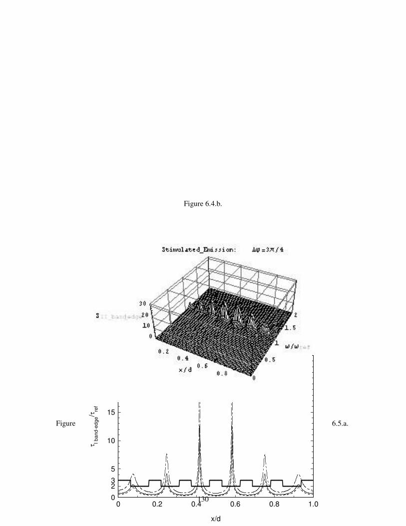
130
Figure 6.4.b.
Figure 6.5.a.
0
5
10
15
20
25
23
0 0.2 0.4 0.6 0.8 1.0
refractive indexSpontaneous Emission(vacuum fluctuations)Stimulated Emission(laser-beams, ∆ϕ=π/4)Stimulated Emission(laser-beams, ∆ϕ=3π/4)
x/d
τ I ban
d-ed
ge/τ
ref

131
Figure 6.5.a.bis.
Figure 6.5.b.
0
5
10
15
20
25
23
0.3 0.4 0.5 0.6
refractive indexSpontaneous Emission(vacuum fluctuations)Stimulated Emission(laser-beams, ∆ϕ=π/4)Stimulated Emission(laser-beams, ∆ϕ=3π/4)
x/d
τ I ban
d-ed
ge/τ
ref
0
5
10
15
20
25
23
0 0.2 0.4 0.6 0.8 1.0
refractive indexSpontaneous Emission(vacuum fluctuations)Stimulated Emission(laser-beams, ∆ϕ=π/4)Stimulated Emission(laser-beams, ∆ϕ=3π/4)
x/d
t II ba
nd-e
dge/τ
ref

132
Figure 6.5.b.bis.
Figure 6.6.a.
0
5
10
15
20
25
23
0.3 0.4 0.5 0.6
refractive indexSpontaneous Emission(vacuum fluctuations)Stimulated Emission(laser-beams, ∆ϕ=π/4)Stimulated Emission(laser-beams, ∆ϕ=3π/4)
x/d
τ II ba
nd-e
dge/τ
ref

133
Figure 6.6.b.
Figure 6.1. Symmetric quarter-wave (QW) one dimensional (1D) Photonic Band Gap (PBG) structure with λref=1µm as reference wavelength, N=6 periods, consisting of two layers with refractive indices nh=3 and nl=2 and lengths h=λref/4nh and l=λref/4nl. Terminal layers of the
0
5
10
15
0 3.14 6.280
0.5
1.0
1.5
2.0
∆ϕ
τ(stim
ulat
ed) /τ
(spo
ntan
eous
)
T(stim
ulat
ed) /T
(spo
ntan
eous
)
II band-edge
0
5
10
15
0 3.14 6.280
0.5
1.0
1.5
2.0
∆ϕ
τ(stim
ulat
ed) /τ
(spo
ntan
eous
)
T(stim
ulat
ed) /T
(spo
ntan
eous
)
I band-edge
134
symmetric QW 1D-PBG structure with parameters: nh and h=λref/4nh. Length of the 1D-PBG structure: d=N(h+l)+h. In the conservative limit, a dipole can be coupled to just one of the 2N+1 Quasi Normal Modes (QNMs) in the [0, 2ref) range, which can be enumerated, excluding =2ref, as 0,nn = , ]2,0[ Nn ∈ . Figure 6.2. With reference to a dipole embedded inside the symmetric QW 1D-PBG structure of fig. 6.1, spontaneous emission processes are described in terms of the sensitivity functions ( )A
nS [eq. (6.3.1)], plotted as functions of the dimensionless space x/d and the dimensionless frequency /ref . In (a) is depicted the sensitivity function ( )
1A
NS − , for the coupling dipole- 1N − (where the real part of the QNM’s frequency is close to the first transmission peak before the low-frequency band-edge); in (b), the sensitivity function ( )A
NS , for the coupling dipole- N (corresponding to the low-frequency band-edge, being I band-edge/ref = 0.8249); in (c) is depicted the sensitivity function
( )1
ANS + , for the coupling dipole- 1N + (where the real part of the QNM’s frequency is close to the
high-frequency band-edge, being II band-edge/ref = 1.175) and, in (d), the sensitivity function ( )2
ANS + ,
for the coupling dipole- 2N + (corresponding to the first transmission peak after the high-frequency band-edge). Figure 6.3. With reference to the dipole embedded inside the symmetric QW 1D-PBG structure of fig. 6.1, in order to describe for the best the spontaneous emission processes of fig. 6.2, the sensitivity functions ( )A
NS and ( )1
ANS + , with frequencies close to the two band-edges, and ( )
1A
NS − , ( )2
ANS + ,
corresponding to the two next transmission peaks, are plotted, as functions of the dimensionless frequency /ref, when: (a) the dipole is inside the 4th period of the 1D-PBG structure, and it is exactly in the centre x=(d/2)+(/2) of the low-index layer, being =h+l. The sensitivity functions
( )AnS , ]2,0[ Nn ∈ are depicted, when: (b) the dipole is inside the 4th period of the 1D-PBG structure,
and it is exactly in the centre x=d/2 of the high-index layer, being also the centre of the 1D-PBG; (c) the dipole lies on one of the two terminal surfaces x=0 and x=d of the 1D-PBG. Figure 6.4. With reference to a dipole embedded inside the symmetric QW 1D-PBG structure of fig. 6.1, stimulated emission processes can be described in terms of the sensitivity functions ( )B
nS [eq. (6.4.1)], plotted as functions of the dimensionless space x/d and of the dimensionless frequency /ref .The 1D-PBG structure is excited by two counter-propagating laser-beams, mismatched by a phase-difference . The sensitivity function ( )
1A
NS + for the coupling dipole- 1N + (corresponding to the high-frequency band-edge) is depicted, when the two laser beams are nearly in phase, (a) =/4, or nearly opposite in phase, (b) =3/4. Figure 6.5. An excited dipole is embedded inside a symmetric QW 1D-PBG structure with parameters λref=1µm, N=6, nh=3, nl=2, pumped by two counter-propagating field pumps filtered at low-frequency band-edge (fig. 6.5.a.) or at high-frequency band-edge (fig. 6.5.b.). The decay-time τ, in units of the decay-time τref for spontaneous emission when the dipole lies on one terminal surface (x=0) of the 1D-PBG structure [eq.(6.5.2)], is plotted as a function of the dimensionless position x/d of the dipole. Several cases are shown: the spontaneous emission [see eq.(6.5.4)], when the two field pumps describe vacuum fluctuations (); and the stimulated emission [see eq.(6.5.7)], when the two pumps describe two input laser-beams, nearly in phase (− − −) or opposite of phase ( − ). Fig. 6.5.a.bis. (fig. 6.5.b.bis.) is a magnification of fig. 6.5.a. (fig. 6.5.b.) for the decay-time in the 3th and 4th periods of the 1D-PBG.

135
Figure 6.6. The excited dipole, embedded inside the symmetric QW 1D-PBG of fig. 6.1, is pumped by two counter-propagating laser-beams filtered at low-frequency band-edge (fig. 6.6.a.) or at the high-frequency band-edge (fig. 6.6.b.). In order to describe for the best the stimulated emission processes of fig. 6.5, the decay-time for stimulated emission (), in units of the decay-time for spontaneous emission [eq. (6.5.7)], is compared with the dwell-time (− − −) for the two laser-beams, in units of the dwell-time for vacuum fluctuations [eq. (6.5.8)]. The decay-time for stimulated emission and the dwell-time for the two laser-beams are compared on different scales as functions of the phase-difference between the two laser-beams.
Chapter 7
136
Coherent Control of Stimulated Emission inside 1D-PBG structures.
(Strong Coupling regime)
1. Introduction.
It has been demonstrated theoretically [2] and experimentally [2] that emission processes,
which had been believed to be an inherent nature of an atom, can be modified in a cavity whose size
is comparable with the wavelength of the emitted light.
Abrupt changes in the density of states (DOS) and photon localization effects may drastically
modify the emission dynamics [3]. This modification takes the form of long time memory effects
and non-Markovian behaviour in the atom-reservoir interaction. Strong modification in the DOS
can be effected by means of photonic crystals [4][5]. It has been suggested that this would be
accompanied by the inhibition of single-photon emission, classical light localization, a photon-atom
bound state, fractionalized single-atom inversion, and anomalously large vacuum Rabi splitting [6].
Lai et al [7] have rigorously investigated the spontaneous electromagnetic decay of a two-
level atom coupled to a narrow cavity resonance in terms of the (Hermitian) modes of the
”universe” [1] rather then the (dissipative) Quasi Normal Modes (QNM) of the open cavity
[1][2]. Special attention is paid to the strong-coupling regime (atomic line-width Γ nearly equal to
cavity resonance width γ), in which there are significant corrections to the golden rule. In particular,
spontaneous decay is most rapid for intermediate values of the quality factor Q of the cavity
resonance.
In the present chapter, the emission processes in a 1D open cavity are analysed on the basis of the
theory presented in ref. [7]. In particular, the stimulated emission is discussed, in strong coupling
regime, for an atom, embedded inside a 1D-PBG structure, which is pumped by two counter-
propagating laser beams. As in ref. [7], quantum electro-dynamics [2] is applied to model the atom-
e.m. field coupling, by considering the atom a two level system, the e.m. field a superposition of
normal modes, the coupling in dipole approximation, and the equations of motion in Wigner-
Weisskopf’s and rotating wave approximations. With respect to ref. [7], the QNM’a approach [7]-
[10] is adopted for an open cavity, interpreting the local density of states (LDOS) as the local

137
density of probability to excite one QNM of the cavity; so this LDOS depends on the phase
difference of the two laser beams.
As main results of this chapter, the strong coupling regime is defined as the one associated to high
values of the LDOS; according to the results of the literature, the emission probability of the atom
decays with an oscillatory behaviour, so that the atomic emission spectrum is splitted into two
peaks (Rabi splitting); the novelty with respect to previous discussions available in literature is that
the phase difference of the two laser beams allow to produce a coherent control of both the
oscillations for the atomic emission probability and the Rabi’s splitting for the emission spectrum.
The chapter is organized as follows. In section 2, the coupling of an atom to an e.m. field is
modelled via quantum electrodynamics equations; it is retained useful to recall the example of an
atom in the free space. In section 3, the atom is embedded inside a leaky cavity and the emission
processes of the atom are modelled. In section 4, the emission probability of the atom is discussed
in strong coupling regime. In section 5, the emission spectrum of the atom is discussed, also in
terms of its poles. In section 6, some criteria are proposed to design an active delay line. In section
7, the conclusions are reported.
2. Coupling of an atom to an e.m. field.
Let consider, inside a one dimensional (1D) universe [ ] 2, 2 , U x x L L L= ∈ − → ∞ of
refractive index n0, an atom, coupled to an e.m. field in the point 0x U∈ , and an open cavity
( ) 0, , C x x d d L= ∈ < , with an inhomogeneous refractive index n(x).
The atom is quantized as a two level system, oscillating at resonance [1], and the e.m. field is in
terms of the 1D universe modes,
( )
( )
0
0
1( ) exp
, 2
g x i xL
L
λ λ
λ
ω ρ
πω λ λρ
= = ∈
, (7.2.1)
where 0=(n0/c)2, being c the speed of the light in vacuum. The atom is modelled by a not
permanent dipole operator [1] along the polarization direction of the e.m. field, and the coupling
of the atom to the e.m. field by the electric dipole approximation [2].

138
At the initial time (t=0), the atom is prepared in the excited state + and the e.m. field in the
vacuum state 0 0λλ
∞
=−∞
= ∏ . With the above initial conditions, the system evolution may be
described using the basis states listed below, with their corresponding eigen values [7]:
-
, 0 0 ,
,1 1 , , λ λ λ
ε
ε ω λ++ = +
− = − + ∈ . (7.2.2)
where , 0+ denotes the state for which the atom is in the upper state, and no photon exists in any
e.m. mode; and ,1λ− denotes the state for which the atom is in the lower state, one photon exists
in the th e.m. mode, while no photon exists in all the other e.m. modes.
2. 1. Quantum electrodynamics equations.
After a time t>0, the system of the atom coupled to the e.m. field lies on a quantum state
( )tψ which can be calculated on the basis states (7.2.2), applying the quantum principle of
superposition [1], i.e.
( ) ( ) ( ),, 0 ,1t c t c tλ λλ
ψ∞
+ −=−∞
= + + − , (7.2.3)
where are introduced the probability coefficients c+(t) and c-,(t) such that c+(0)=1 and c-,(0)=0.
The rotating wave approximation [2] is assumed. The time evolution equations for the probability
coefficients c+(t) and c-,(t) [7],
( ) ( )
( ) ( )
0 ,21 0 0
,02
0 0
( ) exp2
( ) exp2
dcg x c t i t
dt n
dcg x c t i t
dt n
λλ λ λ
λ
λ λλ λ
µ ω ωε
µ ω ωε
∞+
−=
− ∗+
+ −= − − Ω
− += − − Ω
, (7.2.4)
can be solved, giving the time evolution equation for the probability coefficient c+(t),
( ) ( )( )2 210 0 0
1exp
2
tdc Mc i t d
dt n L λ λλ
ω τ ω τ τε
∞+
+=
= − − Ω −
. (7.2.5)
where 0 is the dielectric constant in vacuum, =h/2, being h the Planck’s constant, and 2
M µ= + − .
A correspondence can be established between the discrete modes of a 1D cavity with length L and
the continuous modes of a boundless universe with infinite length L. The mode spectrum
139
becomes continuous as L, because of ( ) 02 0L dλω π ρ ω∆ = ≈ → , and, in this limit, sums
over discrete quantities are converted to integrals over continuous frequency, i.e.
( )( )0
1 0
1,locd x
L λωσ ω
∞∞
=
, (7.2.6)
where (loc)(x,) is the local density of states (LDOS) which can be interpreted as the density of
probability that the e.m. field, in the point x, is excited on just one eigen-state, oscillating around the
frequency [20]. The range of integration over in the expression (7.2.6) strictly extends only
from 0 to , since the physical frequencies are defined to be positive. However, the range can be
extended from - to without significant errors, since most optical experiments use a narrow band
source B [5], i.e. B<<c being c is the central frequency of the bandwidth B. So, the time
evolution equation (7.2.5) becomes
( ) ( )00
,t
(kernel)dcd S x t c
dtτ τ τ+
+= ⋅ − , (7.2.7)
being S(kernel)(x, t) the kernel function, defined as:
( ) ( ) ( )( )2 2
0 0
, , exp2
(kernel) locMS x t d x i t
nω ωσ ω ω
ε
∞
−∞
= − − − Ω
. (7.2.8)
As from (7.2.8), the kernel function depends very strongly on the LDOS (loc)(x,) which can be re-
interpreted as the photon density of states in the reservoir; in essence, eq. (7.2.8) is a measure of the
photon reservoir’s memory of its previous state, on a time scale of evolution of the atomic system,
so S(kernel)(x, t) can be interpreted as memory kernel of the reservoir.
2. 2. Atom in the free space.
If the atom is localized in a point x0 which is outside the open cavity, i.e. x0<0 and x0>d, then
the LDOS (loc)(x,) is referred to the free space [2], [10] [see eq. (5.2.4)]. In the free space, the
emission probability of the atom decays exponentially,
( ) ( )2
0=exp - , 0c t t t+ Γ ≥ , (7.2.9)
where 0 is the atomic decay rate:
2
0 00 2 2
0 0 0 0
11
4M M
n nρ ρ
ε ε
Γ = Ω +
. (7.2.10)
Since the free space is an infinitely broad photon reservoir (flat spectrum), its response should be
instantaneous and the memory effect, associated with emission dynamics, is infinitesimally short
compared to all times of interest. Such interactions are said to be Markovian [2]. In other words, in

140
the free space, the population of the excite state eventually decay to the ground level, independent
of the strength of a driving field. This is a general result valid for almost any broadband smoothly
varying LDOS.
Introducing the atomic parameter
002
0 0
MR
n
ρε
Γ= ≅Ω
, (7.2.11)
which will be interpreted as degree of coupling, the kernel function (7.2.8) can be re-expressed as:
( ) ( ) ( )( )
0
, , exp2
(kernel) locRS x t d x i tω ωσ ω ω
ρ
∞
−∞
= − ⋅ − − Ω . (7.2.12)
3. Atom inside an open cavity.
Let suppose 0<x0<d, so the atom is embedded in a point x0 of the open and inhomogeneous
cavity with refractive index n(x). If the atom, with resonance , is coupled to the nth QNM,
oscillating at frequency Ren, then the atom - nth QNM coupling is characterized by the frequency
detuning:
Re n
n Rω − Ω∆ = . (7.3.1)
The local density of probability ( )( ) ,locn xσ ω for the nth QNM is linked to the integral one n() by
eq. (6.2.4) and the emission processes of the atom are characterized by a kernel function S(kernel)(x,t)
which can be developed as [eq. (7.2.12)]:
( ) ( ) ( ) ( ) ( )2
0
1, exp 0
2(kernel)n n n
n
RS x t x F x d i t , x x d
Iρ ω ωσ ω ω
ρ
∞
−∞
= − ⋅ − − Ω ∀ < < . (7.3.2)
where (x)=[n(x)/c]2, In denote the usual overlapping integrals, and ( ) ( ) 2 n nf fn n nF x f x= ω
are the normalized QNM’s functions, being n nf f and n respectively the QNM’s norm and
frequencies.
3. 1. Spontaneous emission: DOS corresponding to vacuum fluctuations.
If the open cavity is pumped by vacuum fluctuations, which are filtered at the atomic
resonance , next to nth QNM’s frequency of the cavity (Ren), then the integral density of
probability ( )( )Anσ ω for the nth QNM is expressed by eqs. (6.2.5)-(6.2.6) and the spontaneous

141
emission of the atom is characterized by a time evolution equation [eq.(7.2.7)] where the kernel
function ( ),(kernel)nS x t can be specified as [eq. (7.3.2)]
( ) ( ) ( ) ( )
( )( )
( )
2(kernel) 2,
0
2 2
1, exp
22
Im1 2 exp
2 Re Im
n A n n nn
n
n n
R dS x t x F x K I i t
I
i i i t d
ρπρ
ωπ ω ω ω
π ω ω ω
∞
−∞
= − Ω ⋅
⋅ − −
− +
. (7.3.3)
where Kn is the constant of normalization for ( )( )Anσ ω , given by eq. (6.2.6). It is easy to transform
the following signal x(t) in the Fourier domain [14],
( ) ( )
( )( )
Im Re
22
12
Im1( ) exp( )
2 2 Im Re
n ni t
n
n n
dx t e
dti
X x t i t dt
ω ω
ωωω ωπ π ω ω ω
− +
∞
−∞
=
= = −+ −
. (7.3.4)
Inserting eq.(7.3.4) in eq. (7.3.3), it results the kernel function of the spontaneous emission:
( ) ( ) ( ) ( ) ( )2
,0
1, exp 0
4(kernel)n A n n n n n
RS x t K d I x F x i t , tω ρ ω
ρ= − ⋅ − − Ω ∀ ≥ . (7.3.5)
First applying the “theorem of derivation under the integral sign” [14] to eq. (7.2.7),
( ) ( ) ( )2
,, 02
0
, 0(kernel)tn A(kernel)
n A
Sd cS x t c t d c
dt tτ τ+
+ +
∂= = +
∂ , (7.3.6)
and then deriving in time eq. (7.3.5), sampled in the x0 point,
( ) ( ),, 0 , 0
(kernel)n A (kernel)
n n A
Si S x t , t
tω
∂= − − Ω ≥
∂, (7.3.7)
it results, after some algebra, a second order differential equation in time for the probability of
spontaneous emission:
( ) ( ) ( )
( ) ( )
2
, 02
,0
, 0 0
0 1 0 0
(kernel)n n A
nt
d c dci S x t c t
dt dtdc
c , cdt
ω+ ++
++ −
=
+ − Ω − = =
= ∝ =. (7.3.8)
3. 2. Stimulated emission:
DOS depending on the phase difference of two counter-propagating laser-beams.
If the open cavity is pumped by two counter propagating laser beams with a phase difference
, which are tuned at the atomic resonance , next to the nth QNM’s frequency of the cavity
(Ren), then the density of probability ( )( )Bnσ ω for the nth QNM, corresponding to the two laser
142
beams, is linked to the one ( )( )Anσ ω , due to vacuum fluctuations, by eq (6.2.7), and the stimulated
emission of the atom is characterized by a kernel function ( ),(kernel)nS x t , which can be specified as
[eq. (7.3.3)]
( ) ( ) ( ), ,, , 1 1 cosn(kernel) (kernel)
n B n AS x t S x t ϕ = + − ∆
. (7.3.9)
In terms of the frequency detuning for the atom - nth QNM coupling (7.3.1), the quantity (n-) can
be re-expressed as (n-)=(Ren-)+iImn=Rn+iImn and the second order differential equation
in time for the probability of emission processes as
( ) ( ) ( )2
02 Im , 0 0(kernel)n n n
d c dci R i S x t c t
dt dtω+ +
++ ∆ + − = = . (7.3.10)
4. Emission probability of the atom.
The algebraic equation associated to the Cauchy problem (7.3.10), with initial conditions as in
eq. (7.3.8), i.e.
( ) ( )20Im , 0 0(kernel)
n n np R i p S x tω+ ∆ + + = = , (7.4.1)
is solved by two roots,
( ) ( )
( )0
1,2 2
Im 4 , 01 1
2 Im
(kernel)n n n
n n
R i S x tp
R i
ωω
∆ + = = − ± −
∆ +
, (7.4.2)
which allow to express the particular integral of the differential equation (7.3.10):
( ) ( ) ( )2 11 2
2 1 2 1
exp expp p
c t ip t ip tp p p p+ = −
− −. (7.4.3)
The atom – nth QNM coupling is established in strong coupling regime when the particular integral
(7.4.3) presents an oscillatory behaviour, and then the two roots (7.4.2) of the associated algebraic
equation (7.4.1) are complex conjugated [7].
4. 1. Strong coupling regime.
Let consider the spontaneous emission in order to discuss the atom – nth QNM coupling in
strong regime. Since the following condition is valid,
( )
( )( ) ( )( ) ( )
, 0 0 02
, 0 , ,4
Im
(kernel) A An A n n
n free-space free-spacen n
S x t x xRR
d IR i
σ σσ σω
= Ω Ω< ≅
⋅∆ +, (7.4.4)
the atom – nth QNM coupling is in strong regime if [7]:

143
( )
( )( )( )
, 0 02
, 0 , 14 1
Im
(kernel) An A n
free-spacen n
S x t x
RR i
σσω
= Ω> >
∆ +. (7.4.5)
As from eq. (7.4.5), the strong coupling regime is established when the LDOS ( )( )0 ,A
n xσ Ω inside
the open cavity and sampled at the atomic resonance, in units of the LDOS free-space referred to the
free space, exceeds the inverse of the atomic parameter R [eq. (7.2.11)]; the parameter R can be
interpreted as degree of coupling: in fact, the more R is large, the more eq. (7.4.5) is satisfied.
In strong coupling regime (7.4.5), the two roots (7.4.2) become complex conjugated,
( )1,2 , 0
Im, 0
2(kernel)n nn A
R ip i S x t
ω∆ +≅ − ± = , (7.4.6)
and the particular integral (7.4.3) presents an oscillatory behaviour:
( )
( )( )
( ), 0 , 0
, 0
Imexp
2
Imcosh , 0 sinh , 0
2 , 0
n n
(kernel) (kernel)n nn A n A(kernel)
n A
R ic t i t
R i S x t t i S x t t
S x t
ω
ω
+∆ + ≅ − ⋅
∆ + ⋅ = + = =
. (7.4.7)
In fact [eq. (7.3.5)]: ( ) ( ), 0 , 0, 0 , 0(kernel) (kernel)n A n AS x t s x t= = − = so ( ) ( )cosh cosi ⋅ = ⋅ and
( ) ( )sinh sini i⋅ = ⋅ . The oscillatory behaviour may be interpreted as the emission and re-absorption
of one photon; the net decay rate is then determined by the rate of photon leakage, i.e. |Imn|/2.
Now, let consider the stimulated emission; again the atom – nth QNM coupling can be
discussed in strong regime. If the two counter propagating laser beams have a phase difference ,
the atom – nth QNM coupling is characterized by the kernel function (7.3.9). In hypothesis of strong
coupling, expressed by a condition similar to eq.(7.4.5), the particular integral (7.4.3) presents an
oscillatory behaviour,
( )
( )( )
( ), 0 , 0
, 0
Imexp
2
Imcosh , 0 sinh , 0
2 , 0
n n
(kernel) (kernel)n nn B n B(kernel)
n B
R ic t i t
R i S x t t i S x t t
S x t
ω
ω
+∆ + ≅ − ⋅
∆ + ⋅ = + = =
, (7.4.8)
where ( ), 0 , 0(kernel)n BS x t = is linked to the phase difference by eq. (7.3.9); the number of
oscillations for the atomic emission probability depends on the position of the atom inside the
cavity and can be controlled by the phase-difference of the two laser-beams.
The following condition,
( )1 1 cos 0n ϕ+ − ∆ = , (7.4.9)

144
is verified whether the atom is coupled to an odd QNM, i.e. n=1,3,… and the two laser beams are in
phase, i.e. =0, or the atom is coupled to an even QNM, i.e. n=0,2,… and the two laser beams are
opposite in phase, i.e. =. If eq. (7.4.9) is satisfied, the emission probability is over-damped
inside the whole cavity; in spite of the strong coupling, no oscillation occurs [eq. (7.4.8)]:
( ) ( )22 2
2
, 0
Im Im, 0 0 exp 1
4 2 2n n(kernel) n
n B
RS x t b t t t t
ω ω+
∆ = = = + +
. (7.4.10)
5. Emission spectrum of the atom.
At the initial time (t=0), the atom, located in the point x0, is at the upper state and no photons
exists in any normal mode, i.e. c+(x0,t=0)=1; when the atomic decay has occurred (t=), the
coefficient of probability c-,(x0,t) to find the atom in the lower state, one photon existing in the th
e.m. mode and no photon in all the other modes can be derived from eq. (7.2.4):
( ) ( ) ( ), 0 0 020 0 0
, ( ) , exp2
c x t g x c x t i t dtnλ
λ λ λµ ω ω
ε
∞∗
− +
− += ∞ = − − Ω
. (7.5.1)
In terms of the Laplace transform for the probability coefficient c+(x0,t),
( ) ( ) ( )0 00
1, , exp
2C x s c x t st dt
π
∞
+ += − , (7.5.2)
eq. (7.5.1) is so re-expressed:
( ) ( ), 0 0 020 0
, ( ) 2 ,2
c x t g x C x s inλ
λ λ λµ ω π ω
ε∗
− +
− += ∞ = − = − Ω
. (7.5.3)
If the decay has occurred (t=), the atomic emission spectrum can be defined as the density of
probability that the atom in the point x0 has emitted at the frequency [7],
( ) ( ) ( )2
0 , 01
, ,W x c x tλ λλ
ω δ ω ω∞
−=
= = ∞ − , (7.5.4)
where (t) is the delta distribution of Dirac. Inserting eq. (7.5.3) into eq. (7.5.4), it results:
( ) ( ) ( )2
0 02 210 0
1, 2 ,
2M
W x C x in L λ λ λ
λω ω π ω δ ω ω
ε
∞
+=
= − Ω −
. (7.5.5)
If, according to eq. (7.2.6), sums over discrete quantities are converted to integrals over continuous
frequency, applying the proprieties of the Dirac’s distribution, the emission spectrum (7.5.5) can be
reduced as
( ) ( ) ( ) 2( )0 0 0
0
, , 2 ,2
locRW x K x C x iω ωσ ω π ω
ρ +′= ⋅ − Ω , (7.5.6)

145
being K’ a suitable constant of normalization and (loc)(x,) the local density of states (DOS). The
atomic parameter R is defined in eq. (7.2.11).
The frequency range can be extended from - to without significant errors, since most optical
experiments use a narrow band source [5]; the normalization constant K’ can be derived applying
on the emission spectrum (7.5.6) the condition as density of probability, so expressed:
( )0 , 1W x dω ω = . (7.5.7)
Let suppose 0<x0<d and n(x0)>n0, so that the atom is embedded inside the open cavity with
inhomogeneous refractive index (x)=[n(x)/c]2. The atom, with resonance , is assumed to be
coupled with the nth QNM, oscillating at the frequency Ren; the atom - nth QNM coupling is
characterized by the frequency detuning n of eq. (7.3.1). The normalization condition (7.5.7), for
the atomic emission spectrum Wn(x0,), reduces to:
( )Im
0Im
, 1n
n
nW x d
ω
ω
ω ωΩ+
Ω−
= . (7.5.8)
As from eq. (6.2.4), the local density of probability ( )( ) ,locn xσ ω for the nth QNM is proportional to
the (integral) one n(). Inserting eq. (6.2.4) in eq. (7.5.6), the atomic emission spectrum [eq.
(7.5.6)],
( ) ( ) ( ) 2( ) ( )0 0 0
0
, , 2 ,2
loc nn n n
RW x K x C x iω ωσ ω π ω
ρ +′= ⋅ − Ω , (7.5.9)
is specified as:
( ) ( ) ( ) ( ) ( ) 22 ( )0 0 0 0
0
1, 2 ,
2n
n n n nn
RW x K x F x C x i
Iω ρ ωσ ω π ω
ρ +′= ⋅ − Ω , (7.5.10)
where nK ′ is a normalization constant satisfying eq. (7.5.8).
The emission processes of the atom are characterized by a kernel function ( , )(kernel)nS x t which, in
case of spontaneous emission, can be specified as in eq. (7.3.5), and, for stimulated emission, as in
eq. (7.3.9). Inserting eq. (7.3.5) in eq. (7.5.10), the emission spectrum (7.5.10) reads as:
( ) ( ) ( ) ( ) 2, 00 ( )
02
, 0, 22 ,
(kernel)n An n n
n n n n
S x tW xC x i
K d I K
ω σ ωω π ω
ω +
== − − Ω ′ ⋅
. (7.5.11)
As from eq. (7.5.11), the emission spectrum Wn(x0,) depends on the density of probability n(),
as well as on the initial value of the kernel function ( ), 0 , 0(kernel)n AS x t = .
Laplace transforming the Cauchy problem (7.3.10) with initial conditions as in eq. (7.3.8), it results
[14]:
146
( ) ( ) ( )( )
0 20
Im,
Im , 02 (kernel)n n n
n n n
R iiC x i
R i S x tξ ωξ
ξ ω ξπ++ ∆ += −
+ ∆ + + =, (7.5.12)
where is the shifted frequency (-), being the atomic resonance.
5. 1. Poles of the emission spectrum.
The emission spectrum of the atom can be described in terms of the poles, p1 and p2, which
solve eq. (7.4.1) and are expressed in eq. (7.4.2). In strong coupling regime [eq. (7.4.5)], the atomic
emission spectrum Wn(x0,), function of the shifted frequency =(-), is characterized by two
peaks, approximately centred in the resonances Re p1 and Re p2 and with bandwidths linked to 2Im
p1 and 2Im p2; so, a Rabi’s splitting occurs, being the two peaks separated by:
1 2Re Rep pξ∆ = − . (7.5.13)
Let consider the stimulated emission. Two counter propagating laser beams have a phase
difference , so the emission spectrum Wn(x0,) is described by a kernel function ( ), 0 , 0(kernel)n BS x t =
linked to [see eq. (7.3.9)]; as result, the Rabi’s splitting, besides depending on the position of the
atom inside the cavity, can be controlled by the phase-difference of the two laser-beams.
If the operative condition defined by eq (7.4.9) is almost verified, i.e. ( ), 0 , 0 0(kernel)n BS x t = ≈ , the
spectrum Wn(x0,), function of the pure frequency , is reduced to two almost superimposed
pulses: a Lorentian function centred in the nth QNM’s frequency Ren, with a bandwidth 2Im n,
superimposed to a Dirac’s distribution in the atomic resonance Ren, i.e. [see eqs. (6.2.5) and
(6.2.7)]
( ) ( ) ( ) ( )(1) ( ) (2)0 , II
n n n nW x K Kω σ ω δ ω δ ω≈ + − Ω → − Ω , (7.5.14)
where (1)nK and (2)
nK are normalization constants satisfying condition (7.5.8). In fact, the two poles,
1 and 2, are so simplified [eqs. (7.3.1) and (7.4.1)-(7.4.2)]:
1
2
Re Imn niω ω ωω
≈ +≈ Ω
. (7.5.15)
6. Criteria to design an active delay line.
Let specify a Photonic Crystal (PC) as a symmetric Quarter-Wave (QW) one dimensional
(1D) Photonic Band Gap (PBG) cavity; the Quasi Normal Mode’s (QNM’s) approach has been
applied to this kind of structure in refs. [7] [6] and subsequent papers. Consider a symmetric QW
1D-PBG cavity with parameters λref=1µm, N=5, nh=2, nl=1.5 (fig. 7.1.); a “toy 1D-PBG” cavity is

147
chosen because, it is retained sufficient to discuss some criteria for a design of an active delay line.
Locate an atom in the centre of the 1D-PBG, i.e. x0=d/2 (fig. 7.1.). As discussed in ref. [6], for a
symmetric QW 1D-PBG cavity with ref as reference wavelength and N periods, the [0, 2ref) range
includes 2N+1 QNMs which, excluding =2ref are identified as n , ]2,0[ Nn ∈ . If the atom is
located in the centre x0 of the 1D-PBG cavity, it can be coupled to just one of the QNMs with an
even n: in fact, in the centre of the 1D-PBG, the QNM’s intensity 2nF has a maximum for even
values of n and is almost null for odd value of n.
The active cavity, consisting of the 1D-PBG cavity plus the atom, is characterized by a global
transmission spectrum G(x0,) which is the product between the transmission spectrum of the 1D-
PBG |t()|2 and the emission spectrum W(x0,) of the atom [in units of sec], i.e.
20 0( , ) ( , ) ( )G x W x tω ω ω= [in units of sec]. (7.6.1)
A “density of coupling” (DOC) for the active cavity C(x0,) can be defined as the density of
probability that the atom, embedded in the point x0, is coupled to just one QNM, oscillating around
the frequency ; the DOC C(x0,) [in units of sec2/m] is the product between the DOS () [in
units of sec/m] and the atomic emission spectrum W(x0,). Moreover, an “acceleration of coupling”
vC(x0, ) inside the active cavity can be introduced as:
00 0 0
1 1 v( )a ( , )
( , ) ( , ) ( ) ( , )CC
xx W x W x
ωωσ ω ω σ ω ω
= = = [in units of m/sec2]. (7.6.2)
In order to design the active cavity as an ideal delay line, the input pulse must be retarded with an
high amplification but without any distortion: in a narrow pass band, the global transmission (7.6.1)
must assume an high value and the acceleration of coupling (7.6.2) an almost constant value.
As reported above, the atom embedded in the centre of the symmetric QW 1D-PBG cavity
with N=5 periods (fig. 7.1.) can be coupled only to one QNM, oscillating next to an even
transmission peak n=0,2,…,2N; let suppose that the atom is coupled to the (N+1)th QNM, next to
the high frequency band edge, so the quality factor of the 1D-PBG cavity is
11ImN
N
Qω+
+
Ω= , (7.6.3)
being the resonance frequency of the atom. Assume to be in strong coupling regime; the
directories for the active delay line can be satisfied by a suitable value of the coupling degree,
0RΓ=Ω
, (7.6.4)
being 0 the decay rate of the atom in vacuum, and by a suitable value of the frequency detuning for
the atom - (N+1)th QNM coupling,

148
11
Re NN R
ω ++
− Ω∆ = . (7.6.5)
In case of spontaneous emission, if a perfect tuning is assumed, i.e. N+1=0, the atom oscillates at
the frequency of the (N+1)th QNM, i.e. =ReN+1; there exists (figs. 7.2.a. and 7.2.b.) a suitable
value of the coupling degree R, i.e. R*=0.002506, such that the two poles [eqs. (7.4.2) and (7.3.5)]
of the emission spectrum of the atom are distinct for R>R* but coincident for 0<R<R*. In other
words, for R>R*, a Rabi’s splitting (fig. 7.3.a.) occurs in the atomic emission spectrum [eqs.
(7.5.11)-(7.5.12) and (7.3.5)], and so an oscillatory behaviour (fig. 7.4.a.) is present in the atomic
emission probability [eq. (7.4.7) and (7.3.5)]; however, for 0<R<R*, the emission spectrum consists
of two superimposed peaks, and so the emission probability is over-damped. In order to find a
Rabi’s splitting in strong coupling regime, consistent with experiments (0 ~ |ImN+1|) [20], let
employ the degree of coupling:
11
1N
N
R RQ+
+
= = . (7.6.6)
The two poles of the spontaneous emission spectrum, shifted of the atomic resonance , are
1=0.06383+i0.01770 and 2=-0.06383+i0.01995 in units of ref (figs. 7.2.a. and 7.2.b.). They
describe, in resonance and band width, the two peaks of the emission spectrum, whose maxima are
W1=21.87 and W2=15.66 in units of ref (fig. 7.3.a.). Assuming the emission probability almost
decayed after the second oscillation, the decay time is =94.3 in units of 1/ ref (fig. 7.4.a.). So far,
the active cavity has been designed just as a not ideal optical amplifier; an input pulse is amplified
but distorted: as plotted in figs. 7.5.a. and 7.5.b, in the case of spontaneous emission, there exists a
narrow pass band, i.e. = - (-0.06, 0.06) (in units of ref), where the global transmission
spectrum assumes relative high values, i.e. , 1 min max( , ) (2.881, 14.43)C NG G G+ ∈ = in units of 1/ref,
but the acceleration of coupling is subject to a modulation around the value vC,N+1=0.03445 in units
of ref/vref.
Let consider now the case of stimulated emission; the atom inside the symmetric QW 1D-
PBG cavity is excited by two counter propagating laser beams, so that the active delay line can be
realized adding, as new degree of freedom, the phase difference ∆ϕ of the two laser beams. In case
of stimulated emission, if a perfect tuning is again assumed, i.e. N+1=0, the atom oscillates still at
the frequency of the (N+1)th QNM, i.e. =ReN+1. There exists (figs. 7.2.c. and 7.2.d.) a suitable
range of the phase difference ∆ϕ, i.e. 1 2( , ) (2.747, 3.524)ϕ ϕ∆ ∆ = in units of rads, such that the two
poles [eqs. (7.4.2) and (7.3.9)] of the emission spectrum of the atom are distinct for ∆ϕ<∆ϕ1 and
∆ϕ>∆ϕ2 but coincident for ∆ϕ1 <∆ϕ<∆ϕ2. In other words, for ∆ϕ<∆ϕ1 and ∆ϕ>∆ϕ2, a Rabi’s
splitting (fig. 7.3.a.) occurs in the atomic emission spectrum [eqs. (7.5.11)-(7.5.12) and (7.3.9)], and
149
so an oscillatory behaviour (fig. 7.4.a.) is present in the atomic emission probability [eqs. (7.4.8)
and (7.3.9)]; however, for ∆ϕ1 <∆ϕ<∆ϕ2, the emission spectrum consists of two superimposed
peaks, and so the emission probability is over-damped. As a consequence, the Rabi’s splitting and
the oscillations of the decay time can be controlled by the phase difference of the two laser beams.
In order to obtain an ideal delay line by stimulated emission, the two laser beams must exceed in
quadrature, i.e. ∆ϕ>/2; with respect to spontaneous emission, the emission spectrum is
characterized by a narrower Rabi’s splitting and the emission probability by a longer decay time.
So, the active cavity, consisting of the 1D-PBG plus the atom, acts as an delay line, since the delay
time of the active cavity is linked with the decay time of the atom (ref. [21]). Moreover, as
discussed above, the phase difference must not exceed ∆ϕ1=2.747 (in units of rads), otherwise the
Rabi’s splitting tends to zero; by increasing the phase difference with respect to ∆ϕ /2, in the
time domain, the decay time becomes more long still and, in the frequency domain, the global
transmission (7.6.1) is characterized by an high gain but the acceleration of coupling (7.6.2) by a
much too narrow pass band. So, if ∆ϕ ∆ϕ1, the active cavity acts as a delay line which is active
but not ideal. Let conclude that the 1D-PBG cavity should be pumped by two laser beams
exceeding in quadrature of a tilt angle as:
2 10π πϕ∆ = + . (7.6.7)
The two poles of the stimulated emission spectrum, shifted of the resonance , are
1=0.05205+i0.01787 and 2=-0.05205+i0.01978 (in units of ref) (figs. 7.2.c.and 7.2.d.); with
respect to spontaneous emission, the two poles are nearer by =0.02356. They describe, in
resonance and band width, the two peaks of the stimulated emission spectrum, whose maxima are
W1=14.36 and W2=10.93 (in units of ref) (fig. 7.3.a.); with respect to spontaneous emission, the
two maxima are lower by W1=7.51 and W2=4.73. Assuming the emission probability almost
decayed after the second oscillation, the decay time of stimulated emission is =113.5 (in units of 1/
ref) (fig. 7.4.a.); with respect to spontaneous emission, this time is longer by =19.2. So, the
phase difference of the two laser beams allows to control the decay time of the atom and then the
delay time of the active cavity [21]. Now, a delay line has been designed, but it is not quite ideal.
An input pulse is retarded, amplified but a little distorted; as plotted in figs. 7.5.a. and 7.5.b, with
respect to spontaneous emission, there exists a narrower pass band, i.e. = - (-0.04, 0.04),
where the global transmission spectrum assumes similar values, i.e.
, 1 min max( , ) (3.270, 9.24)C NG G G+ ∈ = (in units of ref), and, above all, the acceleration of coupling is
subject to a slight modulation, now around the value vC,N+1=0.05310 (in units of ref/vref).
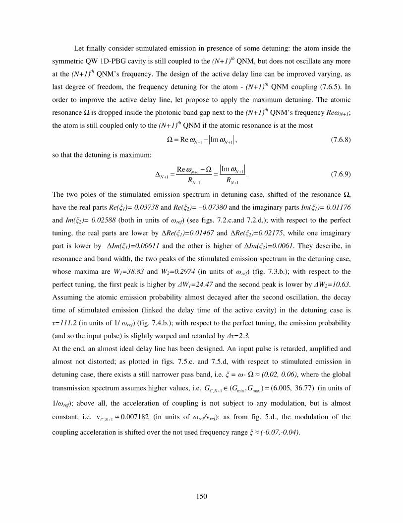
150
Let finally consider stimulated emission in presence of some detuning: the atom inside the
symmetric QW 1D-PBG cavity is still coupled to the (N+1)th QNM, but does not oscillate any more
at the (N+1)th QNM’s frequency. The design of the active delay line can be improved varying, as
last degree of freedom, the frequency detuning for the atom - (N+1)th QNM coupling (7.6.5). In
order to improve the active delay line, let propose to apply the maximum detuning. The atomic
resonance is dropped inside the photonic band gap next to the (N+1)th QNM’s frequency ReN+1;
the atom is still coupled only to the (N+1)th QNM if the atomic resonance is at the most
1 1Re ImN Nω ω+ +Ω = − , (7.6.8)
so that the detuning is maximum:
111
1 1
ImRe NNN
N NR R
ωω +++
+ +
− Ω∆ = = . (7.6.9)
The two poles of the stimulated emission spectrum in detuning case, shifted of the resonance ,
have the real parts Re(1)= 0.03738 and Re(2)= –0.07380 and the imaginary parts Im(1)= 0.01176
and Im(2)= 0.02588 (both in units of ref) (see figs. 7.2.c.and 7.2.d.); with respect to the perfect
tuning, the real parts are lower by Re(1)=0.01467 and Re(2)=0.02175, while one imaginary
part is lower by Im(1)=0.00611 and the other is higher of Im(2)=0.0061. They describe, in
resonance and band width, the two peaks of the stimulated emission spectrum in the detuning case,
whose maxima are W1=38.83 and W2=0.2974 (in units of ref) (fig. 7.3.b.); with respect to the
perfect tuning, the first peak is higher by W1=24.47 and the second peak is lower by W2=10.63.
Assuming the atomic emission probability almost decayed after the second oscillation, the decay
time of stimulated emission (linked the delay time of the active cavity) in the detuning case is
=111.2 (in units of 1/ ref) (fig. 7.4.b.); with respect to the perfect tuning, the emission probability
(and so the input pulse) is slightly warped and retarded by =2.3.
At the end, an almost ideal delay line has been designed. An input pulse is retarded, amplified and
almost not distorted; as plotted in figs. 7.5.c. and 7.5.d, with respect to stimulated emission in
detuning case, there exists a still narrower pass band, i.e. = - (0.02, 0.06), where the global
transmission spectrum assumes higher values, i.e. , 1 min max( , ) (6.005, 36.77)C NG G G+ ∈ = (in units of
1/ref); above all, the acceleration of coupling is not subject to any modulation, but is almost
constant, i.e. , 1v 0.007182C N + ≅ (in units of ref/vref): as from fig. 5.d., the modulation of the
coupling acceleration is shifted over the not used frequency range (-0.07,-0.04).
151
7. Conclusions.
In the present chapter, the stimulated emission has been discussed, in strong coupling
regime, for an atom, embedded inside a one dimensional (1D) Photonic Band Gap (PBG) structure,
which is pumped by two counter-propagating laser beams. Quantum electro-dynamics has been
applied to model the atom-e.m. field coupling, by considering the atom a two level system, the e.m.
field a superposition of normal modes, the coupling in dipole approximation, and the equations of
motion in Wigner-Weisskopf’s and rotating wave approximations. Besides, the Quasi Normal
Mode’s (QNM’s) approach has been adopted for an open cavity, interpreting the local density of
states (LDOS) as the local density of probability to excite one QNM of the cavity; so, this LDOS
depends on the phase difference of the two laser beams. As main results of this chapter, the strong
coupling regime has been defined as the one associated to high values of the LDOS; according to
the results of the literature, the emission probability of the atom decays with oscillatory behaviour,
so that the atomic emission spectrum is splitted into two peaks (Rabi’s splitting); the novelty with
respect to previous discussions available in literature is that the phase difference of the two laser
beams allows to produce a coherent control of both the oscillations for the atomic emission
probability and the Rabi’s splitting for the emission spectrum.
References.
[1] E. M. Purcell, Phys. Rev. 69, 681 (1946); D. Kleppner, Phys. Rev. Lett. 47, 233 (1981).
[2] K. H. Drexhage, Progress in Optics, edited by E. Wolf (North-Holland, New York, 1974), Vol.
12; P. Goy, J. M. Raimond, M. Gross, and S. Haroche, Phys. Rev. Lett. 50, 1903 (1983); R. G.
Hulet, E. S. Hilfer, and D. Kleppner, Phys. Rev. Lett. 55, 2137 (1985); W. Jhe, A. Anderson, E. A.
Hinds, D. Meschede, L. Moi, and S. Haroche, Phys. Rev. Lett. 58, 666 (1987); D. J. Heinzen, J. J.
Childs, J. E. Thomas, and M. S. Feld, Phys. Rev. Lett. 58, 1320 (1987); F. De Martini, G. Innocenti,
G. R. Jacobovitz, and P. Mataloni, Phys. Rev. Lett. 59, 2955 (1987).
[3] S. John, Phys. Rev. Lett. 53, 2169 (1984); S. John, Phys. Rev. Lett. 58, 2486 (1987); E.
Yablonovitch, Phys. Rev. Lett. 58, 2059 (1987); E. Yablonovitch and T. J. Gmitter, Phys. Rev. Lett.
63, 1950 (1989).
[4] J. Maddox, Nature (London) 348, 481 (1990); E. Yablonovitch and K.M. Lenny, Nature
(London) 351, 278, 1991; J. D. Joannopoulos, P. R. Villeneuve, and S. H. Fan, Nature (London)
386, 143 (1997).

152
[5] J. D. Joannopoulos, Photonic Crystals: Molding the Flow of Light (Princeton University Press,
Princeton, New York, 1995); K. Sakoda, Optical properties of photonic crystals (Springer Verlag,
Berlin, 2001); K. Inoue and K. Ohtaka, Photonic Crystals: Physics, Fabrication, and Applications
(Springer-Verlag, Berlin, 2004).
[6] S. John and J. Wang, Phys. Rev. Lett. 64, 2418 (1990); Phys. Rev. B 43, 12772 (1991); S. John,
Confined Electrons and Photons, edited by E. Burstein and C. Weisbuch (Plenum, New York,
1995); R. F. Nabiev, P. Yeh, and J. J. Sanchez-Mondragon, Phys. Rev. A 47, 3380 (1993).
[7] H. M. Lai, P. T. Leung, and K. Young, Phys. Rev. A 37, 1597 (1988).
[8] A. Lahiri, P. B. Pal, A first book of Quantum Field Theory (CRC Press, Calcutta, 2000); C.
Cohen-Tannoudji, J. Dupont-Roc, G. Grynberg Photons and Atoms – Introduction to Quantum
Electrodynamics, (John Wiley, New York, 1997).
[9] P. T. Leung, S. Y. Liu, and K. Young, Phys. Rev. A 49, 3057 (1994); P. T. Leung, S. S. Tong,
and K. Young, J. Phys. A 30, 2139 (1997); P. T. Leung, S. S. Tong, and K. Young, J. Phys. A 30,
2153 (1997); E. S. C. Ching, P. T. Leung, A. Maassen van der Brink, W. M. Suen, S. S. Tong, and
K. Young, Rev. Mod. Phys. 70, 1545 (1998).
[10] K. C. Ho, P. T. Leung, Alec Maassen van den Brink and K. Young, Phys. Rev. E 58, 2965
(1998).
[11] J. J. Sakurai, Advanced Quantum Mechanics (Addison-Wesley, New York, 1995); S.
Weinberg, The Quantum Theory of Fields (Cambridge University Press, New York, 1996).
[12] S. Severini, A. Settimi, C. Sibilia, M. Bertolotti, A. Napoli, A. Messina, Quasi Normal
Frequencies in open cavities: an application to photonic crystals, in press on Acta Phys. Hung. B
(2006).
[13] A. Settimi, S. Severini, N. Mattiucci, C. Sibilia, M. Centini, G. D’Aguanno, M. Bertolotti, M.
Scalora, M. Bloemer, C. M. Bowden, Phys. Rev. E, 68, 026614 (2003).
[14] S. Severini, A. Settimi, C. Sibilia, M. Bertolotti, A. Napoli, A. Messina, Quantum counter-
propagation in open cavities via Quasi Normal Modes approach, submitted to Journal of Laser
Physics (2005).
[15] S. Severini, A. Settimi, C. Sibilia, M. Bertolotti, A. Napoli, A. Messina, Phys. Rev. E 70,
056614 (2004).
[16] A. Settimi, S. Severini, C. Sibilia, M. Bertolotti, M. Centini, A. Napoli, N. Messina, Phys. Rev.
E 71, 066606 (2005).
[17] A. A. Abrikosov, L. P. Gor’kov and I. E. Dzyaloshinski, Methods of Quantum Field Theory in
Statistical Physics (Dover, New York, 1975); P. T. Leung, A. Maassen van den Brink and K.

153
Young, Frontiers in Quantum Physics, Proceedings of the International Conference, edited by S. C.
Lim, R. Abd-Shukor and K. H. Kwek (Springer-Verlag, Singapore, 1998).
[18] K. J. Blow, R. Loudon, S. J. D. Phoenix, and T. J. Shepherd, Phys. Rev A 42, 4102 (1990).
[19] G. F. Carrier, M. Krook, C. E. Pearson, Functions of a complex variable – theory and
technique (McGraw-Hill Book Company, New York, 1983).
[20] S. Hughes and H. Kamada, Phys. Rev. B 70, 195313 (2004).
[21] L. Allen and J. H. Eberly, Optical Resonance and Two-Level Atoms (Dover, New York, 1987);
R. Bonifacio and L. A. Lugiato, Phys. Rev. A 11, 1507 (1975); K. Sakoda and J. W. Haus, Phys.
Rev. A 68, 053809 (2003).
Figures and Captions.
Figure 7.1.
nh nl nh nl nh nl nh nl nh nl nh n0 n0
0 h l x0=d/2 5(h+l) d x
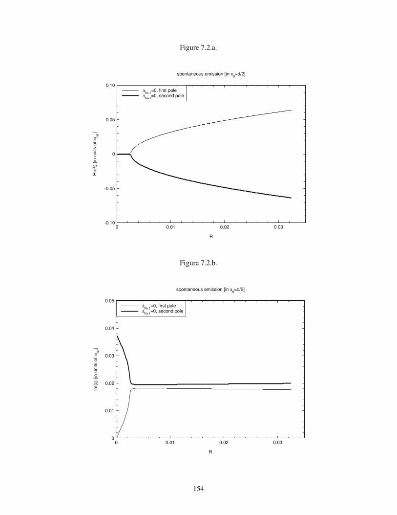
154
Figure 7.2.a.
Figure 7.2.b.
-0.10
-0.05
0
0.05
0.10
0 0.01 0.02 0.03
∆N+1
=0, first pole∆
N+1=0, second pole
R
Re(
ξ) [i
n un
its o
f ωre
f]
spontaneous emission [in x0=d/2]
0
0.01
0.02
0.03
0.04
0.05
0 0.01 0.02 0.03
∆N+1
=0, first pole∆
N+1=0, second pole
R
Im(ξ
) [in
uni
ts o
f ωre
f]
spontaneous emission [in x0=d/2]

155
Figure 7.2.c.
Figure 7.2.d.
0
0.01
0.02
0.03
0.04
0.05
0 3.14 6.28
RN+1
=1/QN+1
, ∆N+1
=0, first poleR
N+1=1/Q
N+1, ∆
N+1=0, second pole
RN+1
=1/QN+1
, ∆N+1
=Im(ωN+1
)/RN+1
, first poleR
N+1=1/Q
N+1, ∆
N+1=Im(ω
N+1)/R
N+1, second pole
∆ϕ
Im(ξ
) [in
uni
ts o
f ωre
f]
stimulated emission [in x0=d/2]
-0.1
0
0.1
0 3.14 6.28
RN+1
=1/QN+1
, ∆N+1
=0, first poleR
N+1=1/Q
N+1, ∆
N+1=0, second pole
RN+1
=1/QN+1
, ∆N+1
=Im(ωN+1
)/RN+1
, first poleR
N+1=1/Q
N+1, ∆
N+1=Im(ω
N+1)/R
N+1, second pole
∆ϕ
Re(
ξ) [i
n un
its o
f ωre
f]
stimulated emission [in x0=d/2]

156
Figure 7.3.a.
Figure 7.3.b.
0
10
20
30
40
-0.2 -0.1 0 0.1 0.2
RN+1
=1/QN+1
, ∆N+1
=0R
N+1=1/Q
N+1, ∆
N+1=Im(ω
N+1)/R
N+1
ξ [in units of ωref
]
WN
+1 (x
0=d/2
) [in
uni
ts o
f ωre
f]
strong coupling [stimulated emission: ∆ϕ=(π/2)+(π/10)]
0
5
10
15
20
25
-0.2 -0.1 0 0.1 0.2
spontaneous emissionstimulated emission [∆ϕ=(π/2)+(π/10)]
ξ [in units of ωref
]
WN
+1 (
x 0=d/2
) [in
uni
ts o
f ωre
f]
strong coupling [RN+1
=1/QN+1
, ∆N+1
=0]
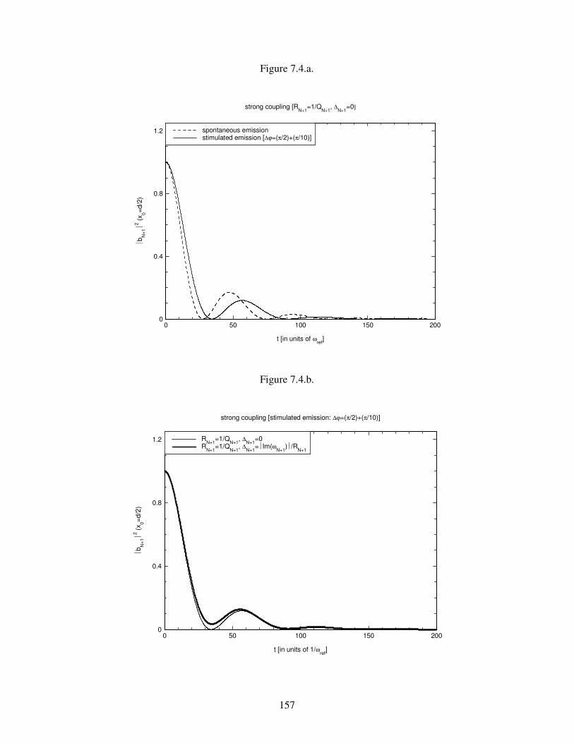
157
Figure 7.4.a.
Figure 7.4.b.
0
0.4
0.8
1.2
0 50 100 150 200
RN+1
=1/QN+1
, ∆N+1
=0R
N+1=1/Q
N+1, ∆
N+1=Im(ω
N+1)/R
N+1
t [in units of 1/ωref
]
bN
+12 (x
0=d/2
)
strong coupling [stimulated emission: ∆ϕ=(π/2)+(π/10)]
0
0.4
0.8
1.2
0 50 100 150 200
spontaneous emissionstimulated emission [∆ϕ=(π/2)+(π/10)]
t [in units of ωref
]
bN
+12 (
x 0=d/2
)
strong coupling [RN+1
=1/QN+1
, ∆N+1
=0]
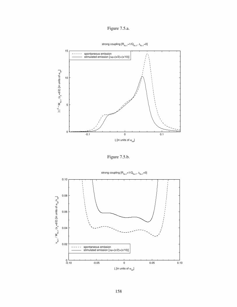
158
Figure 7.5.a.
Figure 7.5.b.
0
0.02
0.04
0.06
0.08
0.10
-0.10 -0.05 0 0.05 0.10
spontaneous emissionstimulated emission [∆ϕ=(π/2)+(π/10)]
ξ [in units of ωref
]
v N+1
/ W
N+1
(x0=d
/2)
[in u
nits
of ω
ref/v
ref]
strong coupling [RN+1
=1/QN+1
, ∆N+1
=0]
0
5
10
15
-0.1 0 0.1
spontaneous emissionstimulated emission [∆ϕ=(π/2)+(π/10)]
ξ [in units of ωref
]
t2 *
WN
+1 (
x 0=d/2
) [in
uni
ts o
f ωre
f]
strong coupling [RN+1
=1/QN+1
, ∆N+1
=0]
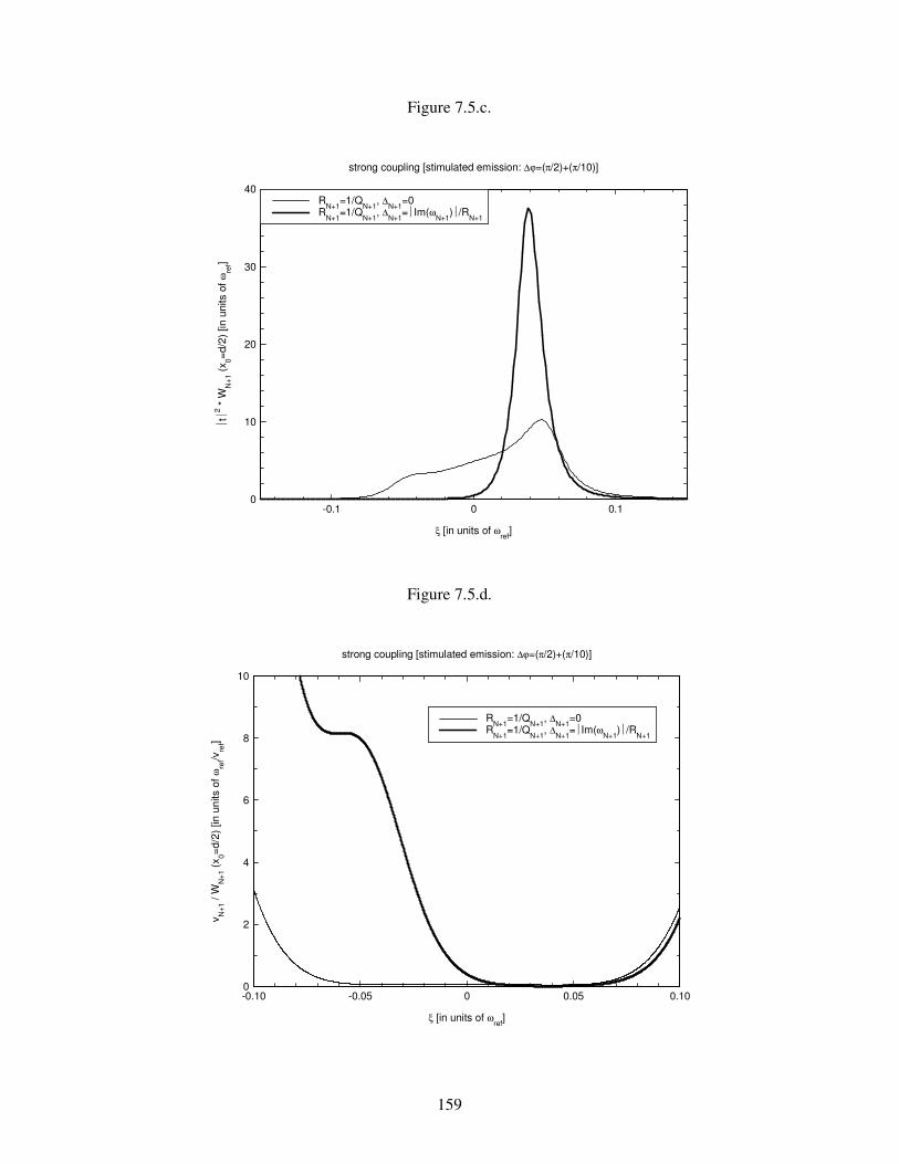
159
Figure 7.5.c.
Figure 7.5.d.
0
2
4
6
8
10
-0.10 -0.05 0 0.05 0.10
RN+1
=1/QN+1
, ∆N+1
=0R
N+1=1/Q
N+1, ∆
N+1=Im(ω
N+1)/R
N+1
ξ [in units of ωref
]
v N+1
/ W
N+1
(x0=d
/2) [
in u
nits
of ω
ref/v
ref]
strong coupling [stimulated emission: ∆ϕ=(π/2)+(π/10)]
0
10
20
30
40
-0.1 0 0.1
RN+1
=1/QN+1
, ∆N+1
=0R
N+1=1/Q
N+1, ∆
N+1=Im(ω
N+1)/R
N+1
ξ [in units of ωref
]
t2 *
WN
+1 (x
0=d/2
) [in
uni
ts o
f ωre
f]
strong coupling [stimulated emission: ∆ϕ=(π/2)+(π/10)]

160
Figure. 7.1. Symmetric Quarter-Wave (QW) one dimensional (1D) Photonic Band Gap (PBG) structure with λref=1µm as reference wavelength, N=5 periods, consisting of two layers with refractive indices nh=2 and nl=1.5 and lengths h=λref/4nh and l=λref/4nl. Terminal layers of the symmetric QW 1D-PBG structure with parameters: nh and h=λref/4nh. Length of the 1D-PBG structure: d=N(h+l)+h. One atom is embedded in the centre of the 1D-PBG, i.e. x0=d/2.
Figure. 7.2. If the atom embedded inside the 1D-PBG structure of fig. 7.1. oscillates at the (N+1)th Quasi Normal Mode (QNM), next to the high-frequency band edge [i.e. in perfect tuning ∆N+1,=0, see eq. (7.6.5)], the spontaneous emission in strong coupling regime can be characterized by the two poles of the emission spectrum of the atom [eqs. (7.4.2) and (7.3.5)], which poles are shifted of the atomic resonance Ω; the real (a) and imaginary (b) parts, in units of the 1D-PBG reference frequency ωref, are plotted as functions of the coupling degree R=Γ0/Ω, which is the ratio between the atomic decay-rate in vacuum Γ0 and the resonance Ω [eq. (7.6.4)]. If two counter-propagating laser beams are tuned at the resonance Ω and the atom is coupled to the (N+1)th QNM, [i.e. QN+1=Ω /Im[ωN+1], see eq. (7.6.3)], the stimulated emission in strong coupling [for RN+1=1/QN+1, eq. (7.6.6)] can be characterized by the two poles of the atomic emission spectrum [eqs. (7.4.2) and (7.3.9)]; whether the atom oscillating at the (N+1)th QNM frequency [i.e. in perfect tuning ∆N+1=0] or at a frequency in the band gap next to the high frequency band edge [i.e. in detuning case ∆N+1=Im[ωN+1]/ RN+1, eq. (7.6.9)], the real (c) and imaginary (d) parts, in units of the 1D-PBG reference frequency ωref, are plotted as functions of the phase difference ∆ϕ between the two laser beams.
Figure. 7.3. Referring to the atom embedded inside the 1D-PBG structure of fig. 7.1, the emission spectrum of the atom, in units of the 1D-PBG reference frequency ωref, is plotted as a function of the dimensionless shifted frequency ξ=(ω-Ω)/ωref. The atom is coupled to the (N+1)th QNM frequency and the emission processes occur in strong coupling regime [for RN+1=1/QN+1]. In tuning hypothesis (a), the atomic emission spectrum for spontaneous processes [eqs. (7.5.11)-(7.5.12)] is compared with the stimulated emission spectrum [eqs. (7.5.11)-(7.5.12)] when the 1D-PBG is pumped by two laser beams with a suitable phase difference: ∆ϕ=(π/2)+(π/10) [eq. (7.6.7)]. In the case of stimulated processes (b) the atomic emission spectrum in perfect tuning is compared with the emission spectrum in detuning case.
Figure. 7.4. Referring to the atom embedded inside the 1D-PBG structure of fig. 7.1, the emission probability of the atom is plotted as a function of the normalized time ωreft. Referring to the operative conditions of fig. 7.3: in tuning hypothesis (a), the atomic emission probability for spontaneous processes [eqs.(7.4.7)] is compared with the stimulated emission probability [eqs. (7.4.8)] when the 1D-PBG is pumped by two laser beams with a suitable phase difference: ∆ϕ=(π/2)+(π/10); in the case of stimulated processes (b), the atomic emission probability in perfect tuning is compared with the emission probability in detuning case.
Figure. 7.5. In order to design a delay line using the active cavity composed of the 1D-PBG structure plus the atom (fig. 7.1.), the delay line can be characterized by a global transmission [eq.(7.6.1)] and by a “coupling acceleration” [eq. (7.6.2)] of the e.m. field; the global transmission, in units of ωref, and the coupling acceleration, in units of ωref/vref, being vref the group velocity of the e.m. field in vacuum, are plotted as functions of the dimensionless shifted frequency ξ=(ω-Ω)/ωref. Referring to the operative conditions of fig. 7.3: in perfect tuning, as from fig. 7.5.a. (fig. 7.5.b.), the global transmission (the coupling acceleration) of the active delay line for spontaneous emission is compared with the global transmission (the coupling acceleration) for stimulated emission when the 1D-PBG is pumped by two laser beams with a suitable phase difference: ∆ϕ=(π/2)+(π/10); in the case of stimulated emission, as from fig. 7.5.c. (fig. 7.5.d.), the global transmission (the coupling acceleration) of the active delay line in perfect tuning is compared with the global transmission (the coupling acceleration) in detuning case.

161

162
DISCUSSION AND CONCLUSIONS
The e.m. field inside an open cavity can be obtained by suitable methods as the transfer
matrix [1] or the ray method [2]. The representation of the e.m. field inside an open cavity can be
given also as a superposition of Quasi Normal Modes (QNMs) which describe the coupling between
the cavity and the environment. The importance of the QNM’s approach lies in the fact that it is
possible to recover the orthogonal representation of the e.m. field, as it is necessary to consider
quantum and non linear processes. Several methods of description for open cavities are discussed in
literature, but the initial hypothesis is different: for example, the QNM’s approach is quite different
from the pseudo-mode’s one introduced by Dalton ed al. in ref. [3]. In fact, the pseudo-modes are
obtained by a Fano’s transformation of the NMs, they are defined as pseudo-modes because they
depend on the external pumping, and they use an ordinary metric; the QNMs are actual modes
because they are defined in absence of an external pumping, and they use a specific definition of
complex metric.
The present Ph-D thesis has examined the properties of a one dimensional (1D) size-limited
optical cavity, subjected to two quantized counter propagating field pumps entering through the two
limiting surfaces of the optical device. The interest is strategically confined to the behaviour of the
leaky cavity in its own and then the environmental field pumps are regarded as assigned external
sources acting upon the optical structure under scrutiny. From a mathematical point of view, this
target has been addressed exploiting the QNM’s approach in a second quantization scheme, here
appropriately extended with the aim of covering the treatment of an open cavity coherently pumped
by noisy field pumps. It is shown that the presence of such pumps may be globally taken into
account by introducing a new physically transparent description of the boundary conditions fulfilled
by the e.m. field inside the cavity. The external counter propagating field pumps are incorporated,
tracing back their effect to that of two assigned electrical currents, existing only on the two limiting
surfaces of the leaky cavity. This method enables to establish, for the first time, a direct link
between the internal QNM’s operators and the external NM’s ones at a generic frequency. The
advantage of such kind of relations stems from the possibility of tracing back the calculation of the
expectation value of any field operator inside an open cavity to that involving only field operators
of the free space. In particular, this route has been followed in order to get the expression of the
auto-correlation function of the e.m. field inside the cavity. The main result of this Ph-D thesis,
beside the introduction of a peculiar language directly stemming from the fact of considering such a
optical device as a forced open quantum system, is to understand the changes provoked by the two
field pumps on some optical properties of the device. Such studies lead to other interesting

163
investigations like, for example, the modified density of states (DOS) inside the optical structure, as
well as the consequent modification of the spontaneous and stimulated emission processes of an
atom placed inside the structure. In order to explore the usefulness of these ideas and mathematical
approach in a physical context of theoretical and applicative interest, the optical device is
specialized as a 1D Photonic Crystal (PC) of finite length.
Non-Hermitian Hamiltonians and the ensuing complex eigen-values figure also in Siegman’s
works on dissipative cavity quantum electro-dynamics (CQED) [4], elaborating Fox and Lee’s
works [5], which consider eigen-value problems for complex symmetric operators. However, refs.
[4] and [5] deal with transverse modes in the semi-classical limit, only considering (a) c-number
fields with some effective quantum noise, and (b) the limit <<d, being the field wavelength and
d the length of the cavity.
The present Ph-D thesis pertains to a different regime. A fully quantum treatment is given for the
dynamics of an atom inside a 1D-PBG, coupled with two counter-propagating laser-beams, by
using the QNM’s approach, i.e. treating the problem in the framework of open systems. As main
result, the decay-time depends from the position of the atom inside the cavity, and can be controlled
by the phase-difference of the two laser-beams. Such a system is relevant for a single-atom, phase-
sensitive, optical memory device on atomic scale.
The strong coupling regime has been defined as the one associated to high values of the local DOS.
According to the results of the literature, the emission probability of the atom decays with
oscillatory behaviour, so that the atomic emission spectrum is splitted into two peaks (Rabi’s
splitting); the novelty with respect to previous discussions available in literature is that the phase
difference of the two laser beams allows to produce a coherent control of both the oscillations for
the atomic emission probability and the Rabi’s splitting for the emission spectrum. Some criteria
have been proposed to design the active cavity consisting of the 1D-PBG plus the atom as an active
delay line: suitable phase differences between the two laser beams allow to obtain a high
transmission in a narrow pass band for a delayed pulse.
This Ph-D thesis paves the way to extend the classic and quantum Quasi Normal Mode’s
theory also in nonlinear optical regime, for two, three dimensional Photonic Crystals and more
general optical devices. In fact, the QNM’s theory is retained the natural approach to study open
cavities, useful to confirm the results of the literature for PBGs in classic ambit and in nonlinear
regime; besides, even if the QNM’s theory may involve boring calculations, it is retained one of the
more effective methods of physical analysis to exam deeper the phenomena of nonlinear cavity
quantum electrodynamics, and then to propose new applications in CQED.

164
[1] M. Born and E. Wolf, Principles of Optics (Macmillan, New York, 1964).
[2] A.W. Crook, J. Opt. Soc. Am. A 38, 954 (1948).
[3] B. J. Dalton, Stephen M. Barnett, and B. M. Garraway, Phys. Rev. A. 64, 053813 (2001).
[4] A. E. Siegman, Phys. Rev. A 39, 1253 (1989); 39, 1264 (1989).
[5] A. G. Fox and T. Li, Bell Syst. Tech. J. 40, 453 (1961).

165
166
RINGRAZIAMENTI Ringrazio il Signore, amico che credevo perso ... Tu mi ha cercato e ritrovato. Ringrazio mia madre Vera...grazie, perché se allora mi avessi ascoltato, ora non sarei un ingegnere, né avrei vissuto gli anni belli del dottorato ... Ho messo a frutto il talento per la ricerca, dono di Dio Padre, perché ho desiderato conoscere le leggi della fisica; ora voglio riconsegnare quel dono nelle mani del Figlio, il Cristo che voglio seguire ed imitare; d’ora in poi, lo Spirito Santo, elargitore di ogni sapienza e scienza, trasfigurerà quel dono perché io possa conoscere sempre più l’Invisibile che è nei cuori di chi andrò a servire. Ringrazio Ilaria, che ha tutti i miei articoli sulla sua scrivania ... grazie, anche se non li leggerai mai. Ringrazio Fernando, per tutte quelle sue parole, a volte burbere, che mi hanno stimolato a crescere ... grazie, perché mi costringi sempre ad ammettere che la saggezza sta in ogni cuore semplice. Ringrazio il professore Bertolotti per l’affetto speciale che mi ha riservato in questi anni, per le sue provocazioni sulle mie presunte virtù cristiane, per tutte le volte che abbiamo quasi bisticciato dopo ogni suo “non capisco”... grazie, anch’io la porto nel cuore in modo speciale, lei è modello di chi mi sarebbe piaciuto essere se Qualcuno non mi avesse chiamato ad altre faccende. Ringrazio Concita, che mi ha raccolto come un seme, quale ero, e mi ha trapiantato in un terreno fertile, non senza la sua preziosa fatica, annaffiandomi con l’acqua degli scontri, spesso duri, necessari perché divenissi uomo prima ancora che ricercatore...grazie, perché anche tu sei diventata la mia buona stella, per tutte le volte che mi hai perdonato quando sono andato oltre le righe e per quando mi hai permesso di condividere ciò che ti preoccupava e che non andava come volevi. Ringrazio Francesco, Roberto, ed Eugenio ... è stato bello vedere la gloria di Dio manifestarsi nella tua vita ... ed ancora Grigore ... scusami davvero per quella volta che pioveva forte e non ti ho lasciato la porta aperta, grazie perché il tuo moto di fastidio mi ha riaperto gli occhi, e qualche tempo dopo in quel tuo dormire di quando stavi male mi sono accorto che la Sua Voce non aveva mai smesso di chiamarmi... Ringrazio il professore Mistura, che ho ammirato per il suo amore verso l’insegnamento ed mi ha accolto come tutore dei suoi ragazzi... grazie perché ho passato momenti piacevoli nella sua stanza, mentre lei mi stimolava in un approccio più meditato verso l’elettromagnetismo. Ringrazio Sergio, amico mio...grazie per le ore che hai voluto passare con me, in cappella universitaria per pregare, in laboratorio nell’arduo compito di costruire una teoria, nei bar chiacchierando davanti a qualche birra, quante risate ... grazie, perché ti ho sempre visto paziente con me, con tutti ed anche di fronte alle delusioni, perché mi hai trasmesso l’amore per la meccanica quantistica e mi consideravi pari a te. Ringrazio Daniela, mia compagna di dottorato ... grazie per tutte le volte che sei cascata nelle mie provocazioni, per la tua bellezza, per il tuo computer, per le chiacchiere ingannando il tempo ... e per la vacanza a S. Pietroburgo, memorabile...

167
Ringrazio Letizia ... credo i primissimi tempi ti risultassi strano, forse perché parlavo troppo di Dio ... poi, quante mattinate passate assieme mentre lavoravi alla tesi mentre io fischiettavo qualche canzoncina irriverente ... mi ricordo che quando arrivavi tu in laboratorio ero felice perché davamo il via alle danze ... grazie per i caffé che non ti ho mai contraccambiato e perché la tua forte personalità mi ha stimolato a crescere in autorevolezza. Ringrazio Marco ... grazie per la tua curiosità verso la mia scelta, per tutte le volte che hai ascoltato i miei sfoghi e per i tuoi consigli, per quando mi hai aiutato con i conti e le simulazioni o anche quando mi dicevi “Ma questo è sbagliato” ... ti ricordi, solo una volta hai sbagliato tu ... io esultavo mentre ti curvavi sul computer, ma vieni!!! Ringrazio Antonio ... grazie, mi sono divertito ai tuoi seminari, anche se non capivo niente, e soprattutto quando mi parlavi delle tue conquiste dell’est ... rimarranno memorabili la sbronza alla cena del Cost e l’abbuffata di salumi e salsicce quelle due notti a Pontinia. Ringrazio Enrico ... la tua generosità è sconfinata ... Raffaella ... grandi sono le tue risorse ... e tutti i ragazzi che hanno messo piede in laboratorio, compreso Alessio che prenderà il mio posto. Ringrazio M. Cristina ... mi hai insegnato la professionalità ... Alessandro ... sei una persona piacevole, anche se a volte ti ho scoperto più integralista di me ... Federico ... sei splendido e ricco di umanità, grazie per il tuo affetto, per i tuoi occhi lucidi e per le tue parole di quando vi ho lasciato... Alessio ... ti ho ammirato per la tua calma e la tua intelligenza che mi metteva in crisi in ogni argomento scientifico e non ... Daniele ... coraggio, rimettiti in piazza, possibile che non ce ne sia una per te tra tutte le fanciulle che ti ronzano attorno?! ... Ringrazio Rosa, il sor Tonnetti ... sei un grande, non mollare mai ... Gioia ... anima dolce, niente ti turbi, niente ti spaventi... Stefania, Liana, e la signora Astengo ... per il suo sorriso.

168


![$VSHWWLWHUPRGLQDPLFLHGLVFDPELRWHUPLFRQHO …padis.uniroma1.it/bitstream/10805/588/1/BoccalettiChiara161.pdf · &kldud%rffdohwwl $vshwwlwhuprglqdplflhglvfdpelrwhuplfrqho ixq]lrqdphqwrghoohpdffklqhiuljrulihuhdgdvvruelphqwr](https://img.dokumen.tips/doc/110x75/5c67528109d3f2ff5a8bb674/vshwwlwhuprglqdplflhglvfdpelrwhuplfrqho-padis-kldudrffdohwwl-vshwwlwhuprglqdplflhglvfdpelrwhuplfrqho.jpg)