Universitat des Saarlandes

UN

IVE R S IT A

S

SA

RA V I E N

SI S

Fachrichtung 6.1 – Mathematik

Preprint Nr. 153

A Shock-Capturing Algorithm for theDifferential Equations of Dilation and Erosion

Michael Breuß and Joachim Weickert

Saarbrucken 2005

Fachrichtung 6.1 – Mathematik Preprint No. 153

Universitat des Saarlandes submitted: Sept. 26, 2005

A Shock-Capturing Algorithm for theDifferential Equations of Dilation and Erosion

Michael Breuß

Technical University BrunswickComputational Mathematics

Pockelsstraße 1438106 Brunswick, Germany

m.breuss@tu-bs.de

Joachim Weickert

Mathematical Image Analysis GroupFaculty of Mathematics and Computer Science

Saarland University66041 Saarbrucken, Germany

weickert@mia.uni-saarland.de

Edited byFR 6.1 – MathematikUniversitat des SaarlandesPostfach 15 11 5066041 SaarbruckenGermany

Fax: + 49 681 302 4443e-Mail: preprint@math.uni-sb.deWWW: http://www.math.uni-sb.de/

Abstract

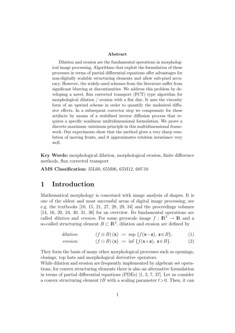
Dilation and erosion are the fundamental operations in morpholog-ical image processing. Algorithms that exploit the formulation of theseprocesses in terms of partial differential equations offer advantages fornon-digitally scalable structuring elements and allow sub-pixel accu-racy. However, the widely-used schemes from the literature suffer fromsignificant blurring at discontinuities. We address this problem by de-veloping a novel, flux corrected transport (FCT) type algorithm formorphological dilation / erosion with a flat disc. It uses the viscosityform of an upwind scheme in order to quantify the undesired diffu-sive effects. In a subsequent corrector step we compensate for theseartifacts by means of a stabilised inverse diffusion process that re-quires a specific nonlinear multidimensional formulation. We prove adiscrete maximum–minimum principle in this multidimensional frame-work. Our experiments show that the method gives a very sharp reso-lution of moving fronts, and it approximates rotation invariance verywell.

Key Words: morphological dilation, morphological erosion, finite differencemethods, flux corrected transport

AMS Classification: 35L60, 65M06, 65M12, 68U10

1 Introduction

Mathematical morphology is concerned with image analysis of shapes. It isone of the oldest and most successful areas of digital image processing; seee.g. the textbooks [10, 15, 21, 27, 28, 29, 34] and the proceedings volumes[14, 16, 20, 24, 30, 31, 36] for an overview. Its fundamental operations arecalled dilation and erosion. For some greyscale image f : IR2 → IR and aso-called structuring element B ⊂ IR2, dilation and erosion are defined by

dilation: (f ⊕ B) (x) := sup {f(x−z), z∈B}, (1)

erosion: (f B) (x) := inf {f(x+z), z∈B}. (2)

They form the basis of many other morphological processes such as openings,closings, top hats and morphological derivative operators.While dilation and erosion are frequently implemented by algebraic set opera-tions, for convex structuring elements there is also an alternative formulationin terms of partial differential equations (PDEs) [1, 2, 7, 37]. Let us considera convex structuring element tB with a scaling parameter t>0. Then, it can

1

be shown that the calculation of u(x, t) = f ⊕ tB and u(x, t) = f tB isequivalent to solving the PDEs

∂tu(x, t) = supz∈B

〈z,∇u(x, t)〉, (3)

∂tu(x, t) = infz∈B

〈z,∇u(x, t)〉, (4)

with f as initial condition [1, 26], respectively. Here, ∇ = (∂x, ∂y)> denotes

the spatial nabla operator, and 〈·, ·〉 is the Euclidean inner product. By choos-ing, e.g., a disc

B :={z ∈ IR2, ‖z‖2 ≤ 1

},

one obtains

dilation: ∂tu = ‖∇u‖2, (5)

erosion: ∂tu = −‖∇u‖2. (6)

The solution at “time” t is the dilation (resp. erosion) of f with a disc ofradius t and center 0 as structuring element.The dilation/erosion PDEs (5)–(6) belong to the class of so-called hyperbolicPDEs, see e.g. [11, 12] to learn more about partial differential equations. Hy-perbolic processes decribe evolutions that propagate information with finitespeed, similar as wave propagation. They may create shocks even if the ini-tial data are smooth, and they require specific numerical schemes that takeinto account the propagation direction and handle shock-like discontinuitiesin a graceful manner [19]. Since many hyperbolic PDEs arise in computa-tional fluid dynamics, it is natural to derive numerical methods for the di-lation/erosion equations from techniques for hyperbolic conservation laws.In particular, finite difference methods such as the Osher–Sethian schemes[22, 23, 32] and the Rouy–Tourin method [25, 38] are widely-used in thiscontext.PDE-based algorithms for dilation/erosion offer two advantages over classicalset-theoretic schemes [2, 8, 26]: first of all, they give excellent results for non-digitally scalable structuring elements whose shapes cannot be representedcorrectly on a discrete grid, for instance discs or ellipses. Secondly, the timet plays the role of a continuous scale parameter. Therefore, the size of astructuring element does not need to be multiples of the pixel size, and it ispossible to get results with sub-pixel accuracy.On the other hand, the main disadvantage of typical PDE-based algorithmsfor mathematical morphology consists of the fact that dissipative effects suchas blurring of discontinuities occur. Apart from an investigation on the use-

2

fulness of high-order ENO1 schemes [33, 35], we are not aware of attemptsin the literature to deal with these undesired numerical diffusion artifacts inPDE schemes for mathematical morphology.It is the goal of the present paper to address this problem. For the develop-ment of our algorithm, we focus on the dilation process (5) since the erosionprocess can be treated analogously. We develop a new variant of the fluxcorrected transport (FCT) technique of Boris and Book [3, 4, 5, 17, 40] in-troduced in the context of fluid flow simulation. Our FCT scheme is used forapproximating one- and two-dimensional morphological processes in an ac-curate and rotationally invariant fashion. The aim of this paper is especiallyto give a detailed derivation and a sound mathematical basis for the 1-D and2-D algorithms.

Related Work. The general idea behind the FCT technique is to compute ina first step the evolution with a scheme that may incorporate much numericaldiffusion. Afterwards, this diffusion is annihilated in a proper fashion by ap-plying a stabilised inverse diffusion step, sometimes also named antidiffusion.In conventional FCT methods, see especially [5], the amount of antidiffusionwhich is to be applied is basically determined by means of the so-called modi-fied equation of the diffusive basis methods, see for instance [13, 19] for detailsconcerning this notion. In some newer works mainly concerned with finite el-ement schemes, antidiffusive fluxes are computed by algebraic properties ofthe entries of corresponding stiffness matrices, see e.g. [18] and the referencestherein. We employ a different approach motivated by the theory of numeri-cal methods for conservation laws, compare e.g. [13]: we construct our FCTscheme considering the viscosity form of the underlying method. By the useof this form we can effectively eliminate the influence of the numerical vis-cosity due to the spatial derivative. It turns out that our scheme provides amuch sharper resolution in comparison with the second-order high-resolutionscheme of Osher and Sethian [23]. Let us note that in contrast to the clas-sical works of Boris, Book and their collaborators, we derive the essentialinformation for our algorithms on the discrete basis, while compared to theapproach of Kuzmin and Turek [18] our proceeding is technically relativelysimple.Furthermore, both mentioned FCT approaches rely on an underlying addi-tive splitting of the backward diffusion into fluxes between computationalnodes: especially in the multidimensional case, the mentioned works proceedalong the considerations of Zalesak [39]. In contrast, our genuinely multidi-

1ENO means essentially non-oscillatory. By adapting the stencil for derivative appro-ximations to the local smoothness of the solution, ENO schemes obtain both high-orderaccuracy in smooth regions and sharp shock transitions.

3

mensional approach yielding directly the desired rotational invariance usesthe dimensional dependent nonlinear form of the numerical viscosity. Thisproceeding is to our knowledge not explored up to now within the literature.However, its usefulness and simplicity is immediately evident in the imageprocessing context presented here.The algorithm we develop in our paper is close in spirit to a recent confe-rence contribution by us, where we developed a FCT approach for three one-dimensional model equations for numerical conservation laws [6]. However,it should be noted that the dilation/erosion PDEs were are investigating inour present paper cannot be written in conservation form, and that we donot restrict ourselves to the 1-D case.

Organisation of the Paper. Our paper is organised as follows. In the nextsection we review some existing numerical schemes for PDE-based mathe-matical morphology. In Section 3 we introduce our novel FCT scheme forthe dilation process in the 1-D case, where we describe the upwind schemeas predictor, and introduce an inverse diffusion algorithm as corrector. Weillustrate its behaviour by an experiment and establish stability results interms of a maximum principle. Section 4 extends these investigations to the2-D case. The paper is concluded with a summary in Section 5.

2 Existing Algorithms

As already meantioned, prominent PDE-based algorithms for the dilationequation are the and the first- and second-order methods of Osher andSethian [22, 23, 32], and the first-order scheme of Rouy and Tourin [25, 38].For the dilation equation

∂tu = ‖∇u‖2 =((∂xu)2 + (∂yu)2

)1/2(7)

the Rouy–Tourin scheme is given by

Un+1i,j = Un

i,j + λ( (

max (0, Uni+1,j−Un

i,j, Uni−1,j−Un

i,j))2

+(max (0, Un

i,j+1−Uni,j, Un

i,j−1−Uni,j)

)2)1/2

, (8)

and the first-order Osher–Sethian upwind scheme can be written as

Un+1i,j = Un

i,j + λ( (

max (0, Uni+1,j − Un

i,j))2

+(max (0, Un

i−1,j − Uni,j)

)2

+(max (0, Un

i,j+1 − Uni,j)

)2+

(max (0, Un

i,j−1 − Uni,j)

)2)1/2

. (9)

4

Thereby, we use as in the following the notation U for discrete data in contrastto the analytical solution u, and we denote the ratio of mesh sizes ∆t and ∆xin t and x direction by λ = ∆t/∆x. We assume that ∆x = ∆y. The upperindex k in Uk

l,m denotes as usual the temporal level k∆t while, analogously,the lower indices l and m specify the spatial mesh point (l∆x, m∆y).As indicated, the mentioned work of Osher and Sethian does not only dealwith first-order upwinding, it also allows high-order approximations in thestyle of high-resolution slope-limiting TVD schemes for conservation laws:for the integration of fluxes accross cell boundaries, the discrete derivativesof grey values are corrected by a contribution taking into account the lo-cal discrete second order derivatives. We refrain from displaying the morecomplicated formulae here.We test the mentioned approaches with a scenario that is sensitive to failuresin the rotational invariance of a method, namely the dilation of a disc. Figure1(a) shows the initial value of the dilation process. The circle is supposed togrow in a uniform fashion while the circular shape is preserved. In Figure1(b) we see the initial image evolved by the Rouy–Tourin algorithm yield-ing a rotationally invariant, but somewhat blurred solution. In Figures 1(c)and (d), we illustrate the behaviour of the first-order Osher-Sethian upwindscheme and the second-order scheme, respectively, using for time integra-tion as proposed in [23] the method of Heun. While both methods seem toappromimate rotational invariance well, we also see that the Osher-Sethianapproach with higher-order resolution does not yield a substantial increasein accuracy. Only within the details one observes a slightly better preser-vation of the circular shape while the circular front is a bit less smeared.This example demonstrates the need for alternative schemes with a bettershock-capturing behaviour.

3 The One-Dimensional FCT Algorithm

We start our one-dimensional investigations in this section with a review ofthe essential properties of an upwind scheme for a general hyperbolic first-order PDE. Afterwards, we derive its specific structure for the case of adilation equation and identify it with the Rouy–Tourin scheme. This schemeserves as first step in our FCT algorithm. In a second step we constructa suitable inverse diffusion step in order to compensate for the numericalviscosity that has been introduced by the upwind scheme. Finally we provea discrete maximum principle for the FCT scheme.

5

Figure 1: (a) Top left: Initial image, 128 × 128 pixels. (b) Top right:Image dilated by the Rouy–Tourin scheme (∆x = ∆y = 1, ∆t = 0.5, 30iterations). (c) Bottom left: Dilated by the first-order upwind scheme (sameparameters). (d) Bottom right: Dilated by a second-order Osher–Sethianscheme (same parameters).

3.1 The General Upwind Scheme in 1-D

The underlying method for our new FCT technique is the classical up-wind scheme. For a general one-dimensional hyperbolic first-order PDE ut +(f(u))x = 0 with f ′(.) ≥ 0 it can be written as

Un+1j = Un

j − λ(

f(Un

j

)− f

(Un

j−1

))

(10)

6

with the notations from the previous section. If f ′(.) < 0 the upwind schemeis given by

Un+1j = Un

j − λ(

f(Un

j+1

)− f

(Un

j

))

. (11)

The upwind scheme has a number of favourable stability properties. Theycan be summarised as follows:

Proposition 3.1 (Stability Properties of the Upwind Scheme)Under the usual CFL stability condition2, the upwind scheme is a local ex-tremum diminishing (LED) scheme. It does not introduce new extrema duringa computation, i.e., it diminishes also the number of extrema (NED proper-ty). Moreover, the upwind scheme satisfies a discrete maximum–minimumprinciple.

The proofs of the validity of the mentioned properties are simple, see forinstance [6, 13] in the context of numerical schemes for conservation laws.

While the upwind scheme can also be shown to approximate the entropysolution3 of the underlying PDE, it has a severe disadvantage: it suffers fromundesirable blurring effects aka numerical viscosity. To quantify these viscousartifacts we write the scheme (10) in its viscosity form, i.e.,

Un+1j = Un

j − λ

2

(

f(Un

j+1

)− f

(Un

j−1

))

(12)

+Qn

j+1/2

2

(Un

j+1 − Unj

)−

Qnj−1/2

2

(Un

j − Unj−1

). (13)

The basic idea behind this decomposition is to consider the part (12) of themethod as a second-order approximation in space (and first order in time)of the underlying process, while part (13) is (in leading order) the discretecounterpart of the numerical diffusion incorporated in the scheme introducedby the spatial approximation.One easily verifies that (10) and (12)–(13) can be made identical by choosingviscosity coefficients Qn

j+1/2 and Qnj−1/2 that satisfy

Qnj+1/2 = λ

fnj+1 − fn

j

Unj+1 − Un

j

and Qnj−1/2 = λ

fnj − fn

j−1

Unj − Un

j−1

(14)

2The Courant–Friedrichs–Lewy (CFL) condition is the fundamental stability criterionfor numerical schemes for hyperbolic PDEs. It requires that the numerical domain ofdependence is included in the analytical domain of dependence of the PDE [9, 19]. Forthe case of the uwind schemes (10) and (11) introduced above, the CFL condition reads∆t max

∣∣f ′

(Un

j

)∣∣, where the maximum is computed over the set

{Un

j

}of all given data.

3An entropy solution is a specific generalised solution, since classical, differentiablesolutions are inappropriate to admit discontinuities that are characteristic for hyperbolicconservation laws.

7

for Unk+1 6= Un

k , k ∈ {j, j − 1}, and f li := f

(U l

i

). By the prerequisite f ′(.) ≥

0 necessary to apply an upwinding in the fashion (10), it is ensured thatthe viscosities Qn

j±1/2 are nonnegative. The resulting numerical diffusion isresponsible for undesirable blurring effects that are observed with this first-order method. Exactly the terms corresponding to (13), (14) will be negatedin a suitable way during a subsquent, stabilised inverse diffusion step of theFCT routine.Let us note that, although the viscosities Qn

j±1/2 in (14) are nonlinear forgeneral f , we will see that in the case of dilation and erosion processes theyare in fact simply constants determined by the chosen space-time mesh. Non-linear effects arise due to the required invariance under rotations as will bediscussed in the section on the 2-D model.

3.2 The FCT Scheme for 1-D Dilation

We now derive the 1-D algorithm for dilation. The corresponding scheme forerosion can be constructed and discussed analogously.

3.2.1 The Formulation of the 1-D Upwind Basis Scheme

Let us define abbreviate notions for the one-sided discrete differences

∆Ukj+1/2 := Uk

j+1 − Ukj (15)

and for the centered discrete differences

∆Ukj := Uk

j+1 − Ukj−1. (16)

In order to clarify the basic idea, let us point out explicitly, that a properscheme describing the dilation process (5) satisfies the following

Principle 3.1 (Discrete Evolution Principle of the Dilation Process)In order to reflect the properties of the analytical dilation operator, the fol-lowing properties need to be satisfied on the discrete level:

• In regions of (strictly) monotone data, the flow is directed from lowerto higher grey values.

• Local minima are increased, while local maxima are maintained.

For the development of our 1-D algorithm, it is useful to fix the attention toa particular spatial index j and to consider a diversion of cases with respect

8

to the data situations one may encounter.

Case I : ∆Unj−1/2 ≥ 0 and ∆Un

j+1/2 > 0.

For this case, the upwind scheme and its viscosity form read

Un+1j = Un

j + λ(Un

j+1 − Unj

)

= Unj +

λ

2

(Un

j+1 − Unj−1

)

︸ ︷︷ ︸

(a)

+λ

2

(Un

j+1 − Unj

)− λ

2

(Un

j − Unj−1

)

︸ ︷︷ ︸

(b)

. (17)

As indicated, (17)(a) is a second-order accurate approximation of ∆t |ux|,while (17)(b) implies Qn

j±1/2 = λ in the investigated case.

Case II : ∆Unj−1/2 < 0 and ∆Un

j+1/2 ≤ 0.

Here the upwind scheme and its viscosity form read

Un+1j = Un

j + λ(Un

j−1 − Unj

)

= Unj +

λ

2

(Un

j−1 − Unj+1

)+

λ

2

(Un

j+1 − Unj

)− λ

2

(Un

j − Unj−1

), (18)

revealing the same structure as in (17), but the approximation of ∆t |ux| isdifferent here.

Case III : ∆Unj−1/2 < 0 and ∆Un

j+1/2 ≥ 0.

The investigated case especially incorporates the situation

∆Unj−1/2 < 0 and ∆Un

j+1/2 > 0,

i.e., a local minimum is located at the index j. Analogously to the proceedingwithin the Rouy–Tourin algorithm [25, 38], we choose the direction of thedilation flow according to the largest gradient, i.e.,

Un+1j

= Unj + λ max

(Un

j+1 − Unj , Un

j−1 − Unj

)

︸ ︷︷ ︸

:=∆Unj

=

{

Unj + λ

2∆Un

j + λ2∆Un

j+1/2 − λ2∆Un

j−1/2 if ∆Unj = Un

j+1 − Unj ,

Unj − λ

2∆Un

j + λ2∆Un

j+1/2 − λ2∆Un

j−1/2 if ∆Unj = Un

j−1 − Unj .

(19)

Note that this choice is not simply a matter of discrete modeling, it is alsoperfectly reasonable since

±λ

2∆Un

j =λ

2

(Un

j±1 − Unj∓1

)≈ ∆t |ux| for ∆Un

j = Unj±1 − Un

j

9

is also a second-order accurate approximation of the dilation process at alocal minimum of the data.

Case IV : ∆Unj−1/2 ≥ 0 and ∆Un

j+1/2 ≤ 0.

Here, according to the formulated Principle 3.1, we set

Un+1j := Un

j . (20)

Summary of Cases I to IV : Having finished the consideration of allpossible cases, we can formulate the upwind scheme as follows:

Un+1j =

Unj for ∆Un

j−1/2 ≥ 0, ∆Unj+1/2 ≤ 0,

Unj + λ

2

∣∣∆Un

j

∣∣ + λ

2∆Un

j+1/2 − λ2∆Un

j−1/2, else.(21)

The scheme (21) is, because of its treatment of local minima, identical withthe 1-D version of the already mentioned Rouy–Tourin method, which isderived in a completely different fashion for the 2-D case. Thereby, for the1-D case, the CFL stability condition reads ∆t ≤ ∆x.By the form (21) we have gained that we can identify the incorporated nu-merical viscosity arising by our approximation of the spatial derivative. Ne-glecting the influence of the first-order temporal approximation, we refer tothe viscosity identified in the above fashion as the numerical viscosity of ourscheme.

In order to illuminate the properties of the method (21), we apply it withoutfurther modification at a simple 1-D test problem depicted in Figure 2. Weclearly observe the desired dilation process, however, the numerical solutionis fairly blurry.

-0.4

-0.2

0

0.2

0.4

0.6

0.8

1

1.2

1.4

-40 -30 -20 -10 0 10 20 30 40-0.4

-0.2

0

0.2

0.4

0.6

0.8

1

1.2

1.4

-40 -30 -20 -10 0 10 20 30 40

Figure 2: Oscillatory initial data and its dilation computed using the de-scribed first-order upwind scheme (21) (∆x = 1, ∆t = 0.2, 30 iterations).

10

3.2.2 The 1-D FCT Step

Now we turn to the FCT methodology. For this, we use in the following thedata notions:

• Un+1/2j for the data obtained by the upwind scheme starting from Un

j ,

• Un+1j for the data obtained after the inverse diffusion step.

When applying an inverse diffusion algorithm, it is evident that one has toincorporate a means of stabilisation. We would like to mention the

Principle 3.2 (of Boris and Book [3]) No antidiffusive flux transfer ofmass can push the density value at any grid point beyond the density valueat neighboring points.

The traditional FCT scheme realises this principle by computing antidiffusivefluxes gj±1/2, so that

Un+1j = U

n+1/2j − gj+1/2 + gj−1/2 (22)

follows. Thereby, Boris and Book use

gj+1/2 := minmod(

∆Un+1/2j−1/2 , ηj+1/2∆U

n+1/2j+1/2 , ∆U

n+1/2j+3/2

)

, (23)

minmod(a, b, c) := sign (b) max(

0, min(sign (b)a, |b|, sign (b)c))

, (24)

where ηj+1/2 is obtained by an analysis of the modified equation, i.e., it isdetermined on the differential level; see especially [5].In 1-D, our proceeding is similar. However, we negate as indicated the diffu-sion computed by the discrete viscosity form introduced before.Thus, we realize Principle 3.2 ensuring the stability of the backward diffusionstep by introducing stabilised inverse diffusion terms of type

gj+1/2 := minmod

(

∆Un+1/2j−1/2 ,

λ

2∆U

n+1/2j+1/2 , ∆U

n+1/2j+3/2

)

(25)

leading here, i.e., in 1-D, to the correction formula

Un+1j = U

n+1/2j − gj+1/2 + gj−1/2. (26)

We can apply our FCT algorithm incorporating (i) the evolution step per-formed by the method (21) and (ii) the correction step (26) again at our 1-Dtest case. For the same computational parameters as before, we see in Fig-ure 3 the initial data together with the solutions obtained using the upwindscheme and the new FCT scheme. Note the significantly sharper resolutionobtained using the latter method while the location of fronts is capturedcorrectly due to the properties of the underlying upwind scheme.

11

-0.4

-0.2

0

0.2

0.4

0.6

0.8

1

1.2

1.4

-40 -30 -20 -10 0 10 20 30 40-0.4

-0.2

0

0.2

0.4

0.6

0.8

1

1.2

1.4

-40 -30 -20 -10 0 10 20 30 40-0.4

-0.2

0

0.2

0.4

0.6

0.8

1

1.2

1.4

-40 -30 -20 -10 0 10 20 30 40

Figure 3: Oscillatory initial data together with the dilation process computedusing (continuous line) the developed upwind scheme, and (dotted line) thenew FCT scheme (∆x = 1, ∆t = 0.2, 30 iterations).

3.2.3 Stability of the 1-D FCT scheme

In the context of morphological dilation processes, useful stability notionsare a global discrete maximum principle as well as a local discrete extremumprinciple. We do not deal explicitly with minima since these are treated bythe construction of the method in the usual fashion, increasing them. Weproceed with the

Proposition 3.2 (Local Extremum Principle)Let

sign(

∆Un+1/2k+1/2

)

= sign(

∆Un+1/2k−1/2

)

6= 0 (27)

hold. Then the FCT scheme defined by

Un+1j = U

n+1/2j − gj+1/2 + gj−1/2 (28)

using g from (25) satisfies locally a discrete maximum–minimum principle:

Un+1j ≥ min

(Un

j−2, Unj−1, Un

j , Unj+1, Un

j+2

)(29)

andUn+1

j ≤ max(Un

j−2, Unj−1, Un

j , Unj+1, Un

j+2

). (30)

Proof. Since the upwind basic scheme satisfies a discrete maximum–minimumprinciple, is is sufficient to show the validity of

Un+1k ∈ conv

(

Un+1/2k−1 , U

n+1/2k , U

n+1/2k+1

)

12

where conv denotes the convex hull.The crucial observation is, that for the assumption (27) the flux contributions

−gj+1/2 and + gj−1/2

defined by (25) have opposite sign, i.e., even if, for instance, in the case

Un+1/2j > U

n+1/2j−1 , we have within the estimation

Un+1/2j −gj+1/2 ≥ U

n+1/2j −∆U

n+1/2j−1/2 = U

n+1/2j −

(

Un+1/2j − U

n+1/2j−1

)

= Un+1/2j−1

in the worst case the validity of the exact equality

Un+1/2j − gj+1/2 = U

n+1/2j−1 .

In any case, the contribution due to +gj−1/2 pushes the resulting value back

into the interior of the convex hull of the values Un+1/2j , U

n+1/2j−1 :

Un+1j = U

n+1/2j − gj+1/2 + gj−1/2

worst case= U

n+1/2j−1 + gj−1/2

︸ ︷︷ ︸

≥0︸ ︷︷ ︸

∈conv“

Un+1/2

j−1, U

n+1/2

j

”

≤ Un+1/2j−1 +

λ

2

(

Un+1/2j − U

n+1/2j−1

)

=

(

1 − λ

2

)

Un+1/2j−1 +

λ

2U

n+1/2j ,

imposing the stability condition λ ≤ 2 which is satisfied for the upwindscheme anyway. The other possible cases can be treated analogously, con-cluding the proof.

Because of the properties of the minmod function, the core of the proof alsoworks without the assumption (27). Thus we can give directly the desired

Corollary 3.1 (Global Maximum Principle)The investigated scheme satisfies globally a discrete maximum principle.

As indicated, the erosion process can be investigated analogously, yielding aglobal discrete minimum principle and a local discrete extremum principle.

13

4 The Two-Dimensional FCT Algorithm

Let us now extend the one-dimensional analysis of the preceding section tothe two-dimensional case. Also here, we only discuss the dilation process indetail.

4.1 The General Upwind Scheme in 2-D

The basis of the 2-D algorithm is a straightforward extension of the 1-Dscheme. Since the underlying PDE reads as

∂tu = ‖∇u‖2 =

√

|∂xu|2 + |∂yu|2, (31)

which, notably, incorporates an additive splitting of the terms constitutedsolely on ux and uy, respectively, we can simply employ the corresponding1 -D upwind expressions to obtain the basic 2 -D upwind scheme for dilationprocesses with a disc.In order to define this scheme, let us give the abbreviations

dUni :=

λ

2

∣∣Un

i+1,j − Uni−1,j

∣∣ +

λ

2

(Un

i+1,j − Unij

)− λ

2

(Un

ij − Uni−1,j

), (32)

dUnj :=

λ

2

∣∣Un

i,j+1 − Uni,j−1

∣∣ +

λ

2

(Un

i,j+1 − Unij

)− λ

2

(Un

ij − Uni,j−1

), (33)

∆Uki,j+1/2 := Un

i,j+1 − Ukij and ∆Uk

i+1/2,j := Uni+1,j − Uk

ij. (34)

Then the scheme reads

Un+1ij =

Unij for ∆Un

i−1/2,j , ∆Uni,j−1/2 ≥ 0 and ∆Un

i+1/2,j , ∆Uni,j+1/2 ≤ 0,

Unij +

√(

dUni

)2

+(

dUnj

)2

, else.

(35)For the scheme (35) again Proposition 3.1 holds, ensuring reasonable proper-ties of the method.As in the 1-D case, one can apply the method (35) without further mo-dification, compare Figure 1. However, as already indicated, any numericalsolution is fairly blurred at the edges incorporated in an image. Note, that therotational invariance of the scheme (35) is obvious due to the considerationof the 2 -norm.For the application of a FCT strategy, it is crucial to observe that there isno general way to extract the discrete viscosity terms out of the square rootin (35). This is exactly the reason why we have to go a different way which

14

distinguishes our scheme from other FCT schemes in the multidimensionalsetting. Note also, that we can now understand that our proceeding in the1-D case has the character of the treatment of a special case: in 1-D, the∂yu-type terms in (35) can be omitted, so that finally – after taking

√

(·)2 –the discrete viscosity terms can be separated directly in an additive fashionfrom the second-order discretisation of |∂xu|.

4.2 The FCT formulation

We proceed in treating the non-maximum case of (35), i.e.,

Un+1ij = Un

ij +

√(

dUni

)2

+(

dUnj

)2

, (36)

in order to derive our 2-D FCT scheme for dilation.Essential for the definition of our FCT procedure is to split a viscous partfrom a second-order part. Thus, we add zero in (36) obtaining

Un+1ij = Un

ij +

√

(dUni )2 +

(dUn

j

)2

+

√(

λ

2

∣∣Un

i+1,j − Uni−1,j

∣∣

)2

+

(λ

2

∣∣Un

i,j+1 − Uni,j−1

∣∣

)2

−

√(

λ

2

∣∣Un

i+1,j − Uni−1,j

∣∣

)2

+

(λ

2

∣∣Un

i,j+1 − Uni,j−1

∣∣

)2

. (37)

Consequently, we now identify the viscous part as

−

√(

λ

2

∣∣Un

i+1,j − Uni−1,j

∣∣

)2

+

(λ

2

∣∣Un

i,j+1 − Uni,j−1

∣∣

)2

+

√

(dUni )2 +

(dUn

j

)2,

while

Un+1ij = Un

ij +

√(

λ

2

∣∣Un

i+1,j − Uni−1,j

∣∣

)2

+

(λ

2

∣∣Un

i,j+1 − Uni,j−1

∣∣

)2

defines the separated (spatial) second-order part.Note that the viscous part is now nonlinear and it cannot be split up addi-tively further into viscous fluxes due to the dimensional influence. For theFCT procedure, it must be handled as one block.

15

Analogously to (32), (33), we now introduce the abbreviations

gi+1/2,j := minmod

(

∆Un+1/2i−1/2,j ,

λ

2∆U

n+1/2i+1/2,j , ∆U

n+1/2i+3/2,j

)

, (38)

gi,j+1/2 := minmod

(

∆Un+1/2i,j−1/2,

λ

2∆U

n+1/2i,j+1/2, ∆U

n+1/2i,j+3/2

)

. (39)

Following then consequently the FCT strategy, we define

Qn+1/2h :=

√(

λ

2

∣∣∣U

n+1/2i+1,j − U

n+1/2i−1,j

∣∣∣

)2

+

(λ

2

∣∣∣U

n+1/2i,j+1 − U

n+1/2i,j−1

∣∣∣

)2

,(40)

Qn+1/2l :=

√(

δUn+1/2i

)2

+(

δUn+1/2j

)2

, (41)

where the stabilised backward diffusive fluxes are incorporated by

δUn+1/2i :=

λ

2

∣∣∣U

n+1/2i+1,j − U

n+1/2i−1,j

∣∣∣ + gi+1/2,j − gi−1/2,j , (42)

δUn+1/2j :=

λ

2

∣∣∣U

n+1/2i,j+1 − U

n+1/2i,j−1

∣∣∣ + gi,j+1/2 − gi,j−1/2, (43)

and we correct the 2-D viscous basis scheme (35) by

Un+1ij = U

n+1/2ij + Q

n+1/2h − Q

n+1/2l (44)

using a notation analogously to the one in the preceeding section.We test our new FCT dilation scheme by considering again the dilation of adisc; see Figure 4 for a comparison with the first-order upwind scheme. Wesee that a significantly sharper resolution of the evolving circle boundaries isobtained.In a second experiment, we consider the real-world test image from Figure5. Also in this case the FCT dilation algorithm gives the desired sharp reso-lution.

4.3 Stability in 2-D

We now investigate the crucial stability properties of the method, meaningthe validity of a local extremum principle and a global discrete maximumprinciple, respectively. As indicated, the major difficulty in the 2-D case isimposed by the nonlinearities due to the dimensional influence in (40)-(43).

Theorem 4.1 (Local Extremum Principle) The described FCT dilationscheme (44) satisfies locally a discrete maximum–minimum principle.

16

Figure 4: (a) Left: Dilation of Figure 1(a), computed by the first-order up-wind scheme (∆x = ∆y = 1, ∆t = 0.5, 30 iterations). (b) Right: Computedby our new FCT scheme (same parameters).

Figure 5: (a) Left: Initial image, 256 × 256 pixels. (b) Right: Dilationcomputed by our new FCT scheme (∆x = ∆y = 1, ∆t = 0.5, 30 iterations).

Proof. It is useful to introduce the abbreviations

αi :=λ

2

∣∣∣U

n+1/2i+1,j − U

n+1/2i−1,j

∣∣∣ , αj :=

λ

2

∣∣∣U

n+1/2i,j+1 − U

n+1/2i,j−1

∣∣∣ , (45)

βi := gi+1/2,j − gi−1/2,j, βj := gi,j+1/2 − gi,j−1/2, (46)

17

for defining the vectors

~α := (αi, αj)T and ~β := (βi, βj)

T . (47)

Using (45)-(47), we can rewrite Qn+1/2h and Q

n+1/2l from (40) and (41) as:

Qn+1/2h = ‖~α‖2, Q

n+1/2l = ‖~α + ~β‖2, (48)

and the updated formula (44) reads

Un+1ij = U

n+1/2ij + ‖~α‖2 − ‖~α + ~β‖2. (49)

Concerning a further analysis of (49), let us point out that we have on theone hand

‖~α‖2 − ‖~α + ~β‖2 = ‖~α + ~β − ~β‖2 − ‖~α + ~β‖2

≤ ‖~α + ~β‖2 + ‖~β‖2 − ‖~α + ~β‖2

= ‖~β‖2, (50)

while we can also easily deduce

‖~α‖2 − ‖~α + ~β‖2 ≥ ‖~α‖2 −(

‖~α‖2 + ‖~β‖2

)

= −‖~β‖2. (51)

Assembling (50) and (51), we obtain

∣∣‖~α‖2 − ‖~α + ~β‖2

∣∣ ≤ ‖~β‖2. (52)

For convenience, let us for the moment assume that

sign(

∆Un+1/2i+1/2,j

)

= sign(

∆Un+1/2i−1/2,j

)

6= 0, (53)

sign(

∆Un+1/2i,j+1/2

)

= sign(

∆Un+1/2i,j−1/2

)

6= 0 (54)

hold. Furthermore, let us consider local data maxima

Un+1/2i+1,j > U

n+1/2ij > U

n+1/2i−1,j and U

n+1/2i,j+1 > U

n+1/2ij > U

n+1/2i,j−1 . (55)

By the construction of the flux function g, see (38) and (39), we can transfer

directly the argument of the proof of Lemma 3.2 in order to see that ‖~β‖2 islimited by

λ

2

√(

Un+1/2i+1,j − U

n+1/2ij

)2

+(

Un+1/2i,j+1 − U

n+1/2ij

)2

. (56)

18

Taking the maximum out of the differences ∆Un+1/2i+1/2,j and ∆U

n+1/2i,j+1/2 occuring

in (56), it follows that the antidiffusive flux contributions can be estimatedvia

λ

2

√2 max

(

Un+1/2i+1,j − U

n+1/2ij , U

n+1/2i,j+1 − U

n+1/2ij

)

, (57)

i.e., we obtain the validity of a local discrete maximum principle under thecondition

λ

2

√2 ≤ 1 ⇔ λ ≤

√2

which is satisfied anyway by the CFL condition of the upwind scheme whichreads in 2-D as λ ≤ 1/

√2.

Remarks

(a) Let us note that, by construction, the proof of Theorem 4.1 can easilybe extended to higher dimensions.

(b) By our derivation of the algorithm and by the proof of Theorem 4.1,it is clear that the crucial restriction imposed on the time step size isdue to the CFL condition for the upwind scheme, and not due to theantidiffusion step.

(c) The above procedure can easily be employed analogously for the erosionprocess; see Figure 6 for computations using the resulting 2-D FCTerosion scheme. Thus, for both dilation and erosion we obtain a discretemaximum–minimum principle as well as a global extremum principle,respectively.

5 Summary and Conclusions

We have presented a novel FCT type algorithm for morphological dilationand erosion processes with a disc as structuring element. It features the de-sirable properties of rotational invariance and sharp resolution. Moreover,the algorithm can easily be extended to a higher-dimensional setting whileretaining these qualities. Technically, we have employed an unconventionalnonlinear genuinely multidimensional formulation of antidiffusive fluxes in or-der to achieve these goals. The resolution of the new method outperforms theRouy-Tourin and Osher-Sethian schemes that are frequently used in PDE-based mathematical morphology. Compared to other FCT approaches thescheme is competitive, while we rely on the discretisation of the underlying

19

Figure 6: (a) Left: Eroded disc using Figure 1 (a) as initial image and ourFCT scheme with ∆x = ∆y = 1, ∆t = 0.5, and 30 iterations. (b) Right:Erosion process with our FCT scheme applied to the Figure 5 (a) as initialimage, here with ∆x = ∆y = 1, ∆t = 0.5, and 10 iterations.

PDE. Our work has addressed the main shortcoming of PDE-based morpho-logical algorithms and makes their resolution at shock fronts comparable toset-based morphological schemes.In our ongoing research we study extensions of this FCT appoach to mor-phological PDEs with other non-digitally scalable structuring elements suchas ellipses.

Acknowledgements. The authors gratefully acknowledge the financial sup-port of their work by the Deutsche Forschungsgemeinschaft (DFG) under thegrants SO 363/9-1 and WE 2602/1-2.

References

[1] L. Alvarez, F. Guichard, P.-L. Lions, and J.-M. Morel. Axioms and fun-damental equations in image processing. Archive for Rational Mechanicsand Analysis, 123:199–257, 1993.

[2] A. B. Arehart, L. Vincent, and B. B. Kimia. Mathematical morphology:The Hamilton–Jacobi connection. In Proc. Fourth International Con-ference on Computer Vision, pages 215–219, Berlin, May 1993. IEEEComputer Society Press.

20

[3] J. P. Boris and D. L. Book. Flux corrected transport. I. SHASTA, afluid transport algorithm that works. Journal of Computational Physics,11(1):38–69, 1973.

[4] J. P. Boris and D. L. Book. Flux corrected transport. III. Minimal errorFCT algorithms. Journal of Computational Physics, 20:397–431, 1976.

[5] J. P. Boris, D. L. Book, and K. Hain. Flux corrected transport. II. Gener-alizations of the method. Journal of Computational Physics, 18:248–283,1975.

[6] M. Breuß, T. Brox, T. Sonar, and J. Weickert. Stabilized nonlinearinverse diffusion for approximating hyperbolic PDEs. In R. Kimmel,N. Sochen, and J. Weickert, editors, Scale-Space and PDE Methods inComputer Vision, volume 3459 of Lecture Notes in Computer Science,pages 536–547, Berlin, 2005. Springer.

[7] R. W. Brockett and P. Maragos. Evolution equations for continuous-scale morphology. In Proc. IEEE International Conference on Acoustics,Speech and Signal Processing, volume 3, pages 125–128, San Francisco,CA, Mar. 1992.

[8] M. A. Butt and P. Maragos. Comparison of multiscale morphologyapproaches: PDE implemented via curve evolution versus Chamfer dis-tance transform. In P. Maragos, R. W. Schafer, and M. A. Butt, editors,Mathematical Morphology and its Applications to Image and Signal Pro-cessing, volume 5 of Computational Imaging and Vision, pages 31–40.Kluwer, Dordrecht, 1996.

[9] R. Courant, K. Friedrichs, and H. Lewy. Uber die partiellen Differen-zengleichungen der mathematischen Physik. Mathematische Annalen,100:32–74, 1928.

[10] E. R. Dougherty. Mathematical Morphology in Image Processing. MarcelDekker, New York, 1993.

[11] L. C. Evans. Partial Differential Equations, volume 19 of GraduateStudies in Mathematics. American Mathematical Society, Providence,1998.

[12] S. J. Farlow. Partial Differential Equations for Scientists and Engineers.Dover, New York, 1993.

21

[13] E. Godlewski and P.-A. Raviart. Hyperbolic Systems of ConservationLaws. Edition Marketing, 1991.

[14] J. Goutsias, L. Vincent, and D. S. Bloomberg, editors. MathematicalMorphology and its Applications to Image and Signal Processing, vol-ume 18 of Computational Imaging and Vision. Kluwer, Dordrecht, 2000.

[15] H. J. A. M. Heijmans. Morphological Image Operators. Academic Press,Boston, 1994.

[16] H. J. A. M. Heijmans and J. B. T. M. Roerdink, editors. Mathemat-ical Morphology and its Applications to Image and Signal Processing,volume 12 of Computational Imaging and Vision. Kluwer, Dordrecht,1998.

[17] D. Kuzmin, R. Lohner, and S. Turek, editors. Flux-Corrected Transport.Springer, Berlin, 2005.

[18] D. Kuzmin and S. Turek. Flux correction tools for finite elements. Jour-nal of Computational Physics, 175:525–558, 2002.

[19] R. J. LeVeque. Finite Volume Methods for Hyperbolic Problems. Cam-bridge University Press, Cambridge, UK, 2002.

[20] P. Maragos, R. W. Schafer, and M. A. Butt, editors. Mathematical Mor-phology and its Applications to Image and Signal Processing, volume 5of Computational Imaging and Vision. Kluwer, Dordrecht, 1996.

[21] G. Matheron. Random Sets and Integral Geometry. Wiley, New York,1975.

[22] S. Osher and R. P. Fedkiw. Level Set Methods and Dynamic ImplicitSurfaces, volume 153 of Applied Mathematical Sciences. Springer, NewYork, 2002.

[23] S. Osher and J. A. Sethian. Fronts propagating with curvature-dependent speed: Algorithms based on Hamilton–Jacobi formulations.Journal of Computational Physics, 79:12–49, 1988.

[24] C. Ronse, L. Najman, and E. Decenciere, editors. Mathematical Mor-phology: 40 Years On, volume 30 of Computational Imaging and Vision.Springer, Dordrecht, 2005.

[25] E. Rouy and A. Tourin. A viscosity solutions approach to shape-from-shading. SIAM Journal on Numerical Analysis, 29:867–884, 1992.

22

[26] G. Sapiro, R. Kimmel, D. Shaked, B. B. Kimia, and A. M. Bruckstein.Implementing continuous-scale morphology via curve evolution. PatternRecognition, 26:1363–1372, 1993.

[27] M. Schmitt and J. Mattioli. Morphologie mathematique. Masson, Paris,1993.

[28] J. Serra. Image Analysis and Mathematical Morphology, volume 1. Aca-demic Press, London, 1982.

[29] J. Serra. Image Analysis and Mathematical Morphology, volume 2. Aca-demic Press, London, 1988.

[30] J. Serra and P. Salembier, editors. Proc. Internationanal Workshopon Mathematical Morphology and its Applications to Signal Processing.Barcelona, Spain, May 1993.

[31] J. Serra and P. Soille, editors. Mathematical Morphology and its Appli-cations to Image Processing, volume 2 of Computational Imaging andVision. Kluwer, Dordrecht, 1994.

[32] J. A. Sethian. Level Set Methods and Fast Marching Methods. CambridgeUniversity Press, Cambridge, UK, second edition, 1999. Paperback edi-tion.

[33] K. Siddiqi, B. B. Kimia, and C.-W. Shu. Geometric shock-capturingENO schemes for subpixel interpolation, computation and curve evolu-tion. Graphical Models and Image Processing, 59:278–301, 1997.

[34] P. Soille. Morphological Image Analysis. Springer, Berlin, second edition,2003.

[35] P. Stoll, C. Shu, and B. B. Kimia. Shock-capturing numerical methodsfor viscosity solutions of certain PDEs in computer vision: The Godunov,Osher–Sethian and ENO schemes. Technical Report LEMS-132, Divisionof Engineering, Brown University, Providence, RI, 1994.

[36] H. Talbot and R. Beare, editors. Proc. Sixth International Symposiumon Mathematical Morphology and its Applications. Sydney, Australia,April 2002. http://www.cmis.csiro.au/ismm2002/proceedings/.

[37] R. van den Boomgaard. Mathematical Morphology: Extensions TowardsComputer Vision. PhD thesis, University of Amsterdam, The Nether-lands, 1992.

23

[38] R. van den Boomgaard. Numerical solution schemes for continuous-scalemorphology. In M. Nielsen, P. Johansen, O. F. Olsen, and J. Weickert,editors, Scale-Space Theories in Computer Vision, volume 1682 of Lec-ture Notes in Computer Science, pages 199–210. Springer, Berlin, 1999.

[39] S. T. Zalesak. Fully multidimensional flux-corrected transport algo-rithms for fluids. Journal of Computational Physics, 31:335–362, 1979.

[40] S. T. Zalesak. Introduction to ”Flux corrected transport. I. SHASTA,a fluid transport algorithm that works”. Journal of ComputationalPhysics, 135:170–171, 1997.

Appendix

For the convenience of the interested reader, we give a brief compilation ofthe 2-D dilation/erosion algorithms.

The Dilation Algorithm

(I) Predictor step with Upwind scheme.Compute Un+1/2 from Un according to (35) with ∆t ≤ 1/

√2.

(II) Corrector step with stabilised inverse diffusion scheme.Compute Uk+1 from Uk+1/2 by (44), thereby assembling the ingredi-ents (38), (39), (42), (43) within (40) and (41).

24

The Erosion Algorithm

(I) Predictor step with Upwind scheme, using instead of (35) but by thesame stability condition as for the dilation scheme:

Un+1ij =

Unij for ∆Un

i−1/2,j , ∆Uni,j−1/2 ≤ 0

and ∆Uni+1/2,j , ∆Un

i,j+1/2 ≥ 0,

Unij −

√(

dUni

)2

+(

dUnj

)2

, else,

where

dUni :=

λ

2

∣∣Un

i+1,j − Uni−1,j

∣∣ − λ

2

(Un

i+1,j − Unij

)+

λ

2

(Un

ij − Uni−1,j

),

dUnj :=

λ

2

∣∣Un

i,j+1 − Uni,j−1

∣∣ − λ

2

(Un

i,j+1 − Unij

)+

λ

2

(Un

ij − Uni,j−1

).

(II) Corrector step with stabilised inverse diffusion scheme.Compute Uk+1 from Uk+1/2 by (44), using the definitions

Qn+1/2h := −

√(

λ

2

∣∣∣U

n+1/2i+1,j − U

n+1/2i−1,j

∣∣∣

)2

+

(λ

2

∣∣∣U

n+1/2i,j+1 − U

n+1/2i,j−1

∣∣∣

)2

,

Qn+1/2l := −

√(

δUn+1/2i

)2

+(

δUn+1/2j

)2

,

with

δUn+1/2i :=

λ

2

∣∣∣U

n+1/2i+1,j − U

n+1/2i−1,j

∣∣∣ − gi+1/2,j + gi−1/2,j ,

δUn+1/2j :=

λ

2

∣∣∣U

n+1/2i,j+1 − U

n+1/2i,j−1

∣∣∣ − gi,j+1/2 + gi,j−1/2.

25