Universal properties of two-dimensional percolation · Universal properties of two-dimensional ... resulting from the perturbation of a CFT by a relevant operator ... In the ﬁrst

SISSA, International School for Advanced Studies

PhD course in Statistical Physics

Academic Year 2011/2012

Universal properties

of two-dimensional

percolation

Thesis submitted for the degree of

Doctor Philosophiae

Advisor:Prof. Gesualdo Delfino

Candidate:Jacopo Viti

17th September 2012

CONTENTS

2

Contents

Summary 5

1 Potts model and percolation 11

1.1 Potts model: FK and domain wall expansions . . . . . . . . . . . . 11

1.2 Basic elements of conformal field theory . . . . . . . . . . . . . . . 15

1.3 Critical q-color Potts model . . . . . . . . . . . . . . . . . . . . . . 21

1.4 A short introduction to percolation . . . . . . . . . . . . . . . . . . 23

1.5 Percolation as the q → 1 limit of the Potts model . . . . . . . . . . 27

2 Potts q-color field theory and the scaling random cluster model 31

2.1 Introduction and general remarks . . . . . . . . . . . . . . . . . . . 31

2.2 Counting correlation functions . . . . . . . . . . . . . . . . . . . . 34

2.2.1 Cluster connectivities . . . . . . . . . . . . . . . . . . . . . 34

2.2.2 Spin correlators . . . . . . . . . . . . . . . . . . . . . . . . . 36

2.2.3 Scaling limit and correlators of kink fields . . . . . . . . . . 40

2.3 Operator product expansions . . . . . . . . . . . . . . . . . . . . . 42

2.4 Duality relations . . . . . . . . . . . . . . . . . . . . . . . . . . . . 48

2.5 The boundary case . . . . . . . . . . . . . . . . . . . . . . . . . . . 52

2.6 Integrable field theories in 1 + 1 dimensions . . . . . . . . . . . . . 56

2.7 Exact solution of the Potts q-color field theory in two dimensions . 60

3 Universality at criticality. The three-point connectivity 73

3.1 Critical three-point connectivity . . . . . . . . . . . . . . . . . . . 73

3.2 Three-point connectivity away from criticality . . . . . . . . . . . . 80

3

CONTENTS

4 Universality close to criticality. Amplitude ratios 834.1 Introduction . . . . . . . . . . . . . . . . . . . . . . . . . . . . . . . 834.2 Two-kink form factors for the spin and kink field . . . . . . . . . . 854.3 The universal amplitude ratios of random percolation . . . . . . . 90

5 Crossing probability and number of crossing clusters away fromcriticality 935.1 Cardy formula for the critical case . . . . . . . . . . . . . . . . . . 935.2 Off-critical percolation on the rectangle . . . . . . . . . . . . . . . 99

5.2.1 Introduction . . . . . . . . . . . . . . . . . . . . . . . . . . 995.2.2 Field theory and massive boundary states . . . . . . . . . . 1005.2.3 Partition functions and final results . . . . . . . . . . . . . 104

6 Density profile of the spanning cluster 1136.1 Statement of the problem and final result . . . . . . . . . . . . . . 1136.2 Derivation. Phase separation in two dimensions . . . . . . . . . . . 114

6.2.1 Introduction . . . . . . . . . . . . . . . . . . . . . . . . . . 1146.2.2 Field theoretical formalism . . . . . . . . . . . . . . . . . . 1166.2.3 Passage probability and interface structure . . . . . . . . . 1206.2.4 Potts model and percolation . . . . . . . . . . . . . . . . . . 123

7 Correlated percolation. Ising clusters and droplets 1277.1 Introduction . . . . . . . . . . . . . . . . . . . . . . . . . . . . . . . 1277.2 Fortuin-Kasteleyn representation . . . . . . . . . . . . . . . . . . . 1307.3 Clusters and droplets near criticality . . . . . . . . . . . . . . . . . 1347.4 Field theory . . . . . . . . . . . . . . . . . . . . . . . . . . . . . . . 138

7.4.1 Integrability . . . . . . . . . . . . . . . . . . . . . . . . . . . 1407.4.2 Connectivity . . . . . . . . . . . . . . . . . . . . . . . . . . 142

7.5 Universal ratios . . . . . . . . . . . . . . . . . . . . . . . . . . . . . 146

Bibliography 155

4

Summary

Percolation was stated as a mathematical problem by Broadbendt and Hammer-sley [1] back in the fifties and is considered by mathematicians [2, 3] a branch ofprobability theory. Due to the large amount of its applications, percolation is apopular subject of research also within the physicist community.1

In its simplest version one takes a regular lattice L and draws bonds connect-ing neighboring sites with probability p. Connected sites form clusters of differentsizes. For p larger than a threshold value pc typical configurations contain a clus-ter with an infinite number of sites, the so-called infinite cluster, which eventuallyfor p = 1 coincides with L itself. The occurrence of the infinite cluster separatestwo different phases, the subcritical phase (p < pc) in which all the clusters arefinite from the supercritical phase (p > pc) in which one is infinite. The phasetransition is continuous and can be described applying concepts like scaling andrenormalization [4, 5], well known to theoretical physicists from the study of crit-ical phenomena. Percolation theory [6] studies the properties of clusters, theiraverage number, their average size and the way in which sites can be distributedamong them (connectivities). It is relevant in the context of complex network[7], polymer gelation [8], diffusion of a liquid in porous media, earthquakes anddamage spreading [9]. Percolation has also been applied in cosmology to modelstar and galaxy formation [10] and in condensed matter problems like the cele-brated quantum Hall effect [11] where the transition is related to the localizationof the electronic wavefunction.

1It is interesting to note that one of the purposes leading Broadbendt and Hammersley to the

introduction of percolation was to test the performance of the computers available at the time.

Nowdays numerical simulations are probably the most efficient way to investigate percolation

from a physicist point of view.

5

SUMMARY

The peculiarity of the percolative phase transition is the absence of any sym-metry breaking mechanism, a circumstance that prevents physicists from writingan effective action for the relevant degrees of freedom in the spirit of Landau andGinzburg. It is however interesting to observe that also the paradigmatic exam-ple of Landau-Ginzburg phase transition, i.e. the spontaneous magnetization of aferromagnet, can be cast in the language of percolation, if one focuses on clustersof equally magnetized spins.

In this thesis we will study the percolative transition in two dimensions, con-centrating on those aspects of the process which do not depend on the specific lat-tice realization and are therefore termed universal. Universality is a consequenceof renormalization group theory. Near criticality, in a system with infinitelymany degrees of freedom, fluctuations of macroscopic observables are stronglyinteracting and correlated on a dynamical length scale, the correlation length,larger than the typical microscopic scale or cut-off. The large distance behaviorof the observables depends on the correlation length and is then unaffected bythe cut-off. At the critical point, where the correlation length diverges, conformalinvariance emerges and the critical behavior of a statistical mechanics model isthen described by a conformally invariant field theory.

In two dimensions [12, 13] conformal field theory (CFT) has been provedextremely useful in providing the classification of the various types of criticalbehaviors occurring in Nature, but even away from criticality the field theoryresulting from the perturbation of a CFT by a relevant operator may have re-markable features. In particular it can possess an infinite number of conservationlaws which strongly constrain the particle dynamics and allow the exact solutionof the scattering problem. Such field theories are called integrable [14, 15].

In this thesis we show how conformal invariance and integrability 2 allow toimprove our understanding of the percolative phase transition and in particular

2During the days in which this thesis was written the 2011 ICTP Dirac medal has been

awarded to E. Brezin, J. Cardy and A. Zamolodchikov “for recognition of their independent

pioneering work on field theoretical methods to the study of critical phenomena and phase

transitions; in particular for their significant contributions to conformal field theories and inte-

grable systems. Their research and the physical implications of their formal developments have

had important consequences in classical and quantum condensed matter systems and in string

theory.”

6

SUMMARY

to derive exact or extremely accurate results, which have been tested by high-precision numerical simulations. The material presented in this thesis is basedon the research articles

• Potts q-color field theory and the scaling random cluster model [16];

• On the three-point connectivity in two-dimensional percolation [17];

• Universal amplitude ratios of two-dimensional percolation from field theory[18];

• Crossing probability and number of crossing clusters in off-critical percola-tion [19];

• Phase separation and interface structure in two dimensions from field theory[20];

• Universal properties of Ising clusters and droplets near criticality [21].

In the first chapter we will introduce the q-color Potts model [22, 23], ageneralization of the well known Ising model invariant under color permutations.After a brief overview of percolation theory, we describe how the percolative phasetransition can be studied formally analyzing the ferromagnetic phase transition ofthe Potts model in the limit q → 1. We will also recall some basic elements of CFTand will give the definition of percolative interface, a concept that mathematicians[24] use to rigorously formulate the physicist notion of scaling limit and conformalinvariance.

The connection between percolation and the Potts model is based on the For-tuin and Kasteleyn representation of the partition function [25], which providesan analytic continuation of the Potts partition function to arbitrary real q, knownas the random cluster model3 [26]. The random cluster model (RCM) undergoesa percolative transition for q less than a dimensionality dependent value qc andthe second chapter is devoted to investigate how its scaling limit can be describedby a field theory, which we call Potts field theory [16]. In particular we will find

3The random cluster model is a percolation model in which bonds are not independent

random variables.

7

SUMMARY

a systematic way to express connectivities in the RCM as spin correlation func-tions in the Potts field theory. Focusing on the bidimensional case we will alsointroduce the concept of kink field: kinks are the lightest excitations interpo-lating between vacua of different colors in the ordered ferromagnetic phase. Thechapter ends with the solution of Chim and Zamolodchikov [27] for the scatteringproblem and with a brief discussion of how correlation functions can be computedout of criticality through the form factor approach.

Chapter 3 is devoted to the three-point connectivity at criticality. In the lan-guage of conformal field theory, percolation is a logarithmic theory, i.e. a theorywith vanishing central charge in which correlation functions may have logarithmicsingularities [28, 29]. We will argue how a formal use of permutational symmetryallows to keep track of the right multiplicities of the kink fields as q → 1 andto determine their operator product expansion (OPE). At criticality the bulkthree-point connectivity factorizes into the product of a constant R and of two-point connectivities. The constant R is exactly the structure constant arising inthe OPE of the kink fields. We determined R exactly [17] also exploiting Al.Zamolodchikov [30] analytic continuation of the structure constants of the con-formal minimal models. Our theoretical result has been confirmed by a numericalsimulation [31].

In chapter 4 we present the computation based on the form factor approach ofall the independent universal amplitude ratios of percolation [18]. In particularwe obtain the ratio between the average size of finite clusters below and abovethe percolation threshold pc. The numerical estimations for this quantity hadbeen controversial for thirty years.

The study of percolation on a finite domain of the plane has also an interestinghistory, started by the observation of Langlands et al. [32] of the universality ofthe vertical crossing probability in the scaling limit on a rectangular geometry andfurther developed by the exact computation by Cardy at the critical point [33].In chapter 5 we recall Cardy derivation of the crossing probability and presentan off-critical extension valid in the limit in which both sides of the rectangleare large compared to the correlation length [19]. Our asymptotic formula agreeswith the numerical data of [34].

In chapter 6 we discuss the density profile of the spanning cluster starting

8

SUMMARY

from the more general perspective of phase separation [20].As we observed at the beginning of this introduction a ferromagnetic transi-

tion is naturally associated to a percolative transition. Naively one would expectthat the existence of a spontaneous magnetization implies the presence of an in-finite cluster of equally magnetized spins and viceversa. The relation betweenmagnetic and geometric degrees of freedom in a ferromagnet is however moresubtle and it is the subject of the final chapter of the thesis where universalproperties of correlated percolation in the Ising model are analyzed [21].

9

SUMMARY

10

Chapter 1

Potts model and percolation

In this chapter we introduce the q-color Potts model on arbitrary graphs G,discussing the Fortuin-Kasteleyn and domain wall representations of the partitionfunction. After a brief overview of conformal field theories in two dimensions, weintroduce basic notions of percolation theory and state the connection with theq → 1 limit of the Potts model.

1.1 Potts model: FK and domain wall expansions

Consider a planar connected graph L ≡ (V,E) of vertex set V and edge setE and associate to any vertex x ∈ V a color variable s(x) = 1, . . . , q ∈ N. Twovertices x, y are nearest neighbors if they are connected by an edge and a pair ofnearest neighboring vertices is denoted by 〈x, y〉. The Potts model Hamiltonian[22, 23] is defined on L by

HPotts = −J∑

〈x,y〉δs(x),s(y) (1.1)

where δs(x),s(y) is the usual Kronecker symbol. The Hamiltonian (1.1) is invariantunder global permutations σ ∈ Sq, the symmetric group of q elements, acting onthe graph variables. The partition function is the sum

ZPotts(J, q) =∑

s(x)e−HPotts . (1.2)

11

CHAPTER 1. POTTS MODEL AND PERCOLATION

For J positive the model is ferromagnetic, antiferromagnetic otherwise.We discuss two convenient ways of rewriting the Boltzmann weight in (1.2),

leading to different graph expansions for the partition function. Take

eJδs(x),s(y) =

[eJ − 1

]δs(x),s(y) + 1[

1− δs(x),s(y)

]+ eJδs(x),s(y).

(1.3)

In both cases the partition function is a product of 2|E(L)| terms, where |E(L)| isthe number of edges in L. Consider the first case and define p = 1− e−J , v = eJ .To any term in the product we associate a graph G ⊆ L, the edges of G coincidewith the edges 〈x, y〉 for which the term containing δs(x),s(y) has been selected inthe expansion, we have

ZPotts(J, q) = v|E(L)| ∑

s(x)

∑

G⊆Lp|E(G)|(1− p)|E(L)|−|E(G)|, (1.4)

where, due to the Kronecker delta, the variables s(x) are constrained to be equalin any connected component1 (cluster) of G. Denoting with |C(G)| the numberof such connected components we obtain


G⊆Lp|E(G)|(1− p)|E(L)|−|E(G)|q|C(G)|, (1.5)

which is called the high temperature or Fortuin-Kasteleyn (FK) graph expansion[25]. The FK expansion provides an analytic continuation of the Potts partitionfunction for q ∈ R; the statistical mechanics model defined by the (1.5) for q > 0is the random cluster model. The graphs entering the FK representation are theFK graphs; notice that two different FK clusters separated by a single edge canhave equal color. Such situation is forbidden by the second choice of rewriting theBoltzmann weight in (1.3), which in turns leads to the domain wall expansion.

First define the dual graph L∗ = (V ∗, E∗) of L. The vertices of L∗ are thecenters of the faces (planar regions) of L and edges of L∗ cross the edges of L, seeFig. 1.1. If the term

[1−δs(x),s(y)

]is chosen, the variables s(x) and s(y) must have

different colors and we draw an edge in the dual graph L∗, intersecting the edge〈x, y〉 ∈ L, see Fig. 1.1. To any graph variable configurations is then associated

1Isolated vertices count as single connected components.

12


Figure 1.1: Left. A graph L and its dual L∗. The vertices of L are the blue dots,the vertices of L∗ are the red circles. Right. A domain wall configuration on thedual lattice L∗ of a square lattice. The graph H∗ contains domain walls enclosingthe clusters of equally colored lattice variables.

a graph H∗, the faces of H∗ are clusters of equally colored graph variables. Thesum over s(x) gives the chromatic polynomial2 πH(q) of H the dual graph of H∗and we obtain the domain wall representation of the Potts model [35]

ZPotts(J, q) = v|E(L)|∑

H∗πH(q)v−length(H∗), (1.6)

where length(H∗) is the total length of H∗ domain walls.Assume J > 0. When v À 1 the formation of domain walls is suppressed in

(1.6) and typical configurations have uniform colorations. On the other hand forv ¿ 1 and p→ 0 (1.5) shows that FK clusters with few sites are more probable.The sum over their possible colors produces typically a permutational invariantconfiguration. Let |V (L)| the number of vertices of L. In the thermodynamiclimit |V (L)| → ∞ one expects the existence of a graph dependent, and thennon-universal, value Jc such that for q smaller than a dimensionality dependentvalue qc(d) the model has a continuous (second order) phase transition [23] andthe free energy

FPotts(J, q) = − log ZPotts(J, q), (1.7)

2The chromatic polynomial of a graph is the number of possible colorations of the vertices of

the graph such that each vertex may have q different colors and adjacent vertices have different

colors.

13


0.0 0.2 0.4 0.6 0.8 1.0

0.0

0.2

0.4

0.6

0.8

1.0

e-J

e-J*

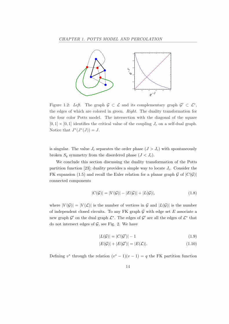
Figure 1.2: Left. The graph G ⊂ L and its complementary graph G′ ⊂ L∗,the edges of which are colored in green. Right. The duality transformation forthe four color Potts model. The intersection with the diagonal of the square[0, 1] × [0, 1] identifies the critical value of the coupling Jc on a self-dual graph.Notice that J∗(J∗(J)) = J .

is singular. The value Jc separates the order phase (J > Jc) with spontaneouslybroken Sq symmetry from the disordered phase (J < Jc).

We conclude this section discussing the duality transformation of the Pottspartition function [23]; duality provides a simple way to locate Jc. Consider theFK expansion (1.5) and recall the Euler relation for a planar graph G of |C(G)|connected components

|C(G)| = |V (G)| − |E(G)|+ |L(G)|, (1.8)

where |V (G)| = |V (L)| is the number of vertices in G and |L(G)| is the numberof independent closed circuits. To any FK graph G with edge set E associate anew graph G′ on the dual graph L∗. The edges of G′ are all the edges of L∗ thatdo not intersect edges of G, see Fig. 2. We have

|L(G)| = |C(G′)| − 1 (1.9)

|E(G)|+ |E(G′)| = |E(L)|. (1.10)

Defining v∗ through the relation (v∗ − 1)(v − 1) = q the FK partition function

14


(1.5) is3

ZPotts(J, q) = (v − 1)|E(L)|q1−|V (L∗)| ∑

G′⊆L∗(v∗ − 1)|E(G′ )|q|C(G′ )|. (1.11)

Apart from a prefactor the partition function ZPotts(J, q) on the graph L coin-cides with the partition function ZPotts(J∗, q) on the dual graph L∗. The dualitytransformation J∗(J) is shown in Fig. 1.2 and maps the partition function onL at small coupling J ¿ 1 into the partition function on L∗ at large couplingJ∗ À 1. If now L is a self-dual graph, for example a bidimensional square lattice,the fixed point of the duality map J∗(Jc) = Jc is the value of the coupling forwhich the model is critical. For q < qc, approaching Jc the variables s(x) becomecorrelated on larger and larger length scales and their fluctuations do not dependon the lattice details. This feature, termed universality4, is a consequence ofthe renormalization group on which we will come back in the next section andchapters of the thesis.

1.2 Basic elements of conformal field theory

Figure 1.3: Three examples of conformal transformations in the complex plane.From left to right are drawn in the z plane the curves Re(w) = const and Im(w) =const for the mappings w(z) = 1

z ,√

z and log z.

We recall some basic results of conformal field theory in two dimensions. Let Lbe a regular lattice with lattice spacing a and H

(s(x), J) the Hamiltonian of

3We used |L(L)| = |V (L∗)| − 1 and |C(L)| = 1.4More precisely, different statistical mechanics models share the same properties at large

distances on the critical surface identified by the irrelevant directions of the renormalization

group transformation.

15


a statistical mechanics model formulated in terms of variables s(x) and couplingset J. The two-point correlation function is the average

〈s(x)s(0)〉 =1Z

∑

s(x)e−Hs(x)s(0). (1.12)

Near the critical point the behavior of (1.12)

〈s(x)s(0)〉 = ξ−2XsF(|x|/ξ

)(1.13)

defines the correlation length ξ, the typical length scale of the fluctuations and Xs

the scaling dimension5 of s(x). ξ diverges at criticality and the region of validity of(1.13) is the scaling region. In the scaling region the functional form (1.13) is notaffected6 by the specific details of the lattice L and we can identify renormalizedlocal densities (scaling fields), for example φ(x) ∼ a−Xss(x), whose conjugatedcouplings transform multiplicatively under the linearized renormalization grouptransformation [4, 5]. In the continuum limit a→ 0 the dynamics of the densitiesis described by an Euclidean two-dimensional quantum field theory

〈φ(x)φ(0)〉S =1Z

∫Dφ e−S[φ]φ(x)φ(0), (1.14)

with action S specified by the requirement that for |x| À a

〈s(x)s(0)〉 = K〈φ(x)φ(0)〉S , (1.15)

where K is an a-dependent normalization constant. The mass of the quantumfield theory m is the inverse of ξ. At the fixed point of the renormalization grouptransformation ξ = ∞ and the densities φi(x) with scaling dimension Xφi obeyglobal scale invariance under x→ bx

φi(bx) = b−Xφi φ(x). (1.16)

The corresponding quantum field theory has action S∗ and it is massless, withtwo-point function

〈φi(x)φi(0)〉S∗ =1

|x|2Xφi

, (1.17)

5In d dimensions for a scalar order parameter 2Xs = d − 2 + η with η the usual anomalous

dimension.6F (t) → e−t + const. in the infrared limit |x| À ξ and F (t) → t−2Xφ in the ultraviolet limit

|x| ¿ ξ.

16


which is a power-law. In writing (1.17) we also assumed rotational and trans-lational invariance; if we further require the invariance of S∗ under local scaletransformations x → b(x)x the full group of symmetry is the conformal groupand S∗ is conformal invariant [36].

Restrict from now on to two dimensions [12]. Conformal transformations ofcoordinates maintain local angles between vectors in the plane, see Fig. 1.3. Forconvenience we introduce complex coordinates z = x1 + ix2 and z = x1 − ix2,the Euclidean metric g = 1

2

[dz ⊗ dz + dz ⊗ dz

]is off-diagonal in the coordinates

(z, z) and therefore the tangent vectors ∂ ≡ ddz and ∂ ≡ d

dz have zero norm. Thetransformation of coordinates w(z, z) preserves the angles if

〈∂w, ∂w〉 = 〈∂w, ∂w〉 = 0, (1.18)

〈∂w, ∂w〉 =12Ω(w, w), (1.19)

where ∂w ≡ ddw , ∂w ≡ d

dw and the inner product 〈a, b〉 between two vectors a, b isg(a, b). It is simple to prove that (1.18) and (1.19) are satisfied by the isogonalmappings w(z, z) = w(z) and w(z, z) = w(z) giving Ω(w, w) =

∣∣ dzdw

∣∣2. Howeveronly analytic functions preserve the local angle orientation and define a conformalmapping.

The scaling fields for which the requirement of conformal covariance analogousto (1.19) naturally translates into

φi(w, w) =∣∣∣∣dz

dw

∣∣∣∣Xφi

φi(z, z) (1.20)

are the primary fields of the conformal field theory. Conformal transformationsare analytic functions and it is useful to regard z and z as independent variablesdefining two different scaling dimensions hφi , hφi such that Xφi = hφi + hφi .Under z → w(z), z → w(z) a primary field transforms as

φi(w, w) =(

dz

dw

)hφi(

dz

dw

)hφi

φi(z, z). (1.21)

The real numbers hφi and hφi are equal for a scalar field and are called confor-mal dimensions. An infinitesimal conformal transformation w(z) = z + ε(z) isgenerated by the stress energy tensor Tµν(x), which is symmetric, traceless and

17


Hout

inH

inH

Hout

1t

t2

1tt2 zw

2 iπR

wz=e

Figure 1.4: Radial quantization of a conformal field theory on the z plane isobtained from the conformal mapping z = e−

2πiwR , where w = x + iy is the

Euclidean coordinate on the cylinder. The asymptotic Hilbert spaces of masslessparticles are denoted by Hin and Hout.

conserved. In complex coordinates Tµν has only two independent componentsTzz = T11 − 2iT12 − T22 ≡ T (z) and Tzz = T11 + 2iT12 − T22 ≡ T (z), whichare purely analytic and antianalytic as a consequence of the conservation law∂µTµν = 0.

To quantize a conformal field theory we introduce light-cone coordinates w± =x ± t and think the Minkowsky space-time as a cylinder of circumference7 R.The asymptotic Hilbert spaces Hin and Hout are defined on the cylinder at timet = ±∞. Operators of the quantum theory Φ(x, t) are of the factorized formΦ+(w+)Φ−(w−) and inside correlation functions time-ordering T is understood

〈Φ1(x1, t1) . . .Φn(xn, tn)〉 ≡ 〈T Φ1(x1, t1) . . .Φn(xn, tn)〉, (1.22)

T Φ1(x1, t1) . . .Φn(xn, tn)

=

∑σ∈Sn

∏n−1i=1 θ(tσ(i)− tσ(i+1))Φσ(1) . . . Φσ(n). After

the analytic continuation t = iy to Euclidean space let w = x + iy. The quan-tization prescription (radial quantization) on the complex plane of z is obtainedexploiting conformal covariance through the mapping z = e−

2iπR

w, see Fig. 1.4.For example, suppose to compute on the z plane the equal times commutator

7This is necessary because a massless field theory on the line has not well defined asymptotic

states.

18


between two operators A(ζ), B(z). Time ordering on the cylinder translates intoradial ordering on the plane and we find

[A(ζ), B(z)] = lim|ζ|→|z|

θ(|ζ| − |z|)A(ζ)B(z)− θ

(|z| − |ζ|)B(z)A(ζ). (1.23)

If the operator A is expressed as a contour integral of some operator density Q(w)at constant time |w| = |ζ|

A =∮

|w|=|ζ|

dw

2πiQ(w), (1.24)

the commutator reads

[A,B(z)] =∮

Cz

dw

2πiQ(w)B(z), (1.25)

where Cz is a contour encircling the point z. To evaluate (1.23) it is necessary toknow the singularities arising from the short distance expansion limw→z Q(w)B(z)which are ruled by the Operator Product Expansion (OPE). Let us consider thestress energy tensor T (z). By dimensional analysis

limw→z

T (w)T (z) =c/2

(w − z)4+

2T (z)(w − z)2

+∂T (z)z − w

+ regular terms, (1.26)

the real parameter c is the central charge of the conformal field theory. Asoperators A and B of the form (1.24) we take the Laurent modes defined as

Ln =1

2πi

∮

CO

dz zn+1T (z), (1.27)

with CO a contour encircling the origin O. The combined use of (1.26) and (1.23)gives the commutation rule

[Ln, Lm] = (n−m)Ln+m +c

12δn+m,0 n(n2 − 1), (1.28)

which defines the Virasoro algebra. Consider now a primary field8 φh(z) withconformal dimension h. Assuming the OPE

limw→z

T (w)φh(z) =hφh(z)

(w − z)2+

∂φh(z)w − z

+ regular terms (1.29)

8We only focus on the dependence from the coordinate z.

19


from (1.23) the commutation relations with the Laurent modes

[Ln, φh(z)] = h(n + 1)znφh(z) + zn+1∂φ(z) (1.30)

follow. The study of the representation theory of the Virasoro algebra (1.28) isequivalent to the characterization of the Hilbert space Hin and we summarize thebasic results [4, 13].

• The Hilbert space Hin is the vector space of an infinite dimensional rep-resentation of the Virasoro algebra. Highest weights |h〉 are eigenvector ofL0 defined by the action of the primary φh(0) on the conformal invariantvacuum |Ω〉. Form (1.30)

L0|h〉 = h|h〉. (1.31)

The vacuum |Ω〉 is the only highest weight with conformal weight h = 0.

• Descendant states of |h〉 are obtained applying the modes L−n, n > 0,to |h〉. The descendant state L−n1 . . . L−nk

|h〉 has L0 eigenvalue h + N ,N =

∑ki=1 ni. N is the level of the descendant and the number of descen-

dant states of |h〉 at level N is P (N), the number of partitions of N intopositive, not necessarily distinct, integers. The set of states resulting fromthe application of the L−n’s to the highest weight |h〉 is the Verma moduleof |h〉. The Hilbert space Hin is a direct sum of Verma modules.

• The P (N) × P (N) matrix resulting from the scalar products of the de-scendant states of |h〉 at level N is the Grahm matrix G(h, c,N). Virasoroalgebra representations are unitary if all the elements of G(h, c, N) are non-negative and irreducible if they are non-vanishing. The classification of theVirasoro algebra representations is based on the exact formula, found byKac, for the determinant of G(h, c, N). We summarize the conclusions.

– For c < 0 there are no unitary representations.

– For c > 1 all the representations are unitary and irreducible for everyvalue of h.

– For c = 1 there are infinite values of h for which the representationsare reducible but all of them are unitary.

20


– For 0 < c < 1 unitary representations are obtained for

c = 1− 6t(t + 1)

, hm,n =[(t + 1)m− tn]2 − 1

4t(t + 1), (1.32)

where t, m and n are integers with t > 2 and m = 1, . . . , t − 1n = 1, . . . ,m. The representations are reducible and irreducible rep-resentations are obtained subtracting all the vectors with vanishingnorm (null vectors) from the Verma module. For a given t, the confor-mal field theory defined by (1.32) is called the minimal modelMt

9. Ina minimal model the null norm condition for a vector generates a dif-ferential equation for the primary correlation functions, which can besolved exactly. The primary fields with conformal dimensions (1.32)are also the generators of the OPE algebra.

1.3 Critical q-color Potts model

The critical Potts model for arbitrary values of q is described by a conformal fieldtheory10. The parameter t in (1.32) relates to q as [37, 38]

√q = 2 sin

π(t− 1)2(t + 1)

. (1.33)

The theory is minimal only for integer q < 4. The value q = 4 corresponds to c = 1and for q > 4 the Potts phase transition is first order (qc(2) = 4). The maximumnumber of colors allowing the existence of a second order phase transition in twodimensions can be found by simple group theoretic considerations, as we willshow in sections 2.3 and 2.7. The conformal dimensions hε and hs for the Pottsthermal and spin fields can be conjectured for arbitrary q [37, 38]

hε = h2,1 =t + 34t

, (1.34)

hs = h t+12

, t+12

=(t + 3)(t− 1)

16t(t + 1). (1.35)

9For c < 0 also exist representations which are minimal, i.e. they contain a finite number of

primaries, but not unitary. The simplest example is the Lee-Yang model.10When q is not integer we are referring to the random cluster model representation of the

partition function.

21


We observe from (1.32) that for q 6= 2, 3 the Verma module of the Potts spinfield s does not contain null vectors and no differential equations are known tobe satisfied by its correlation functions.

As an example of conformal minimal model we discuss the critical three-colorPotts model. The Hamiltonian is

H = −J∑

〈x,y〉

23

[cos

(ϕ(x)− ϕ(y)

)+

12

], (1.36)

where ϕ(x) = 2π3 s(x) and s(x) = 1, 2, 3. It is useful to consider the complex spin

variables σ(x) = eiϕ(x) and σ(x) = e−iϕ(x), in terms of which the Hamiltonian(1.36) shows an explicit S3 = Z3 o Z2 symmetry11, the Z2 factor is associatedto the symmetry σ → σ. In the scaling limit the most relevant fields of thecontinuum theory are the spin field s(x) = σ(x) + σ(x) and the energy fieldε(x). As discussed in section 1.1 the model is critical on a square lattice forJc = log(1 +

√3). A comparison with the critical exponents of the exact lattice

solution due to Baxter [39] allows to identify the critical quantum theory as theminimal modelM5 with central charge 4/5. The primary fields of theM5 theoryare collected with their conformal weights in the Kac table.

n = 4 18

3 115

23

2 140

2140

138

1 0 25

75 3

m 1 2 3 4

Table 1.1: The Kac table for the minimal modelM5. The conformal dimensionshm,n are indicated.

The spin field corresponds to φ3,3 and the energy field to φ2,1. The conformaldimensions in the second row of the table do not have an interpretation in thelattice solution and the corresponding fields decouple from the OPE algebra. The

11The presence of the semi-direct product o is due to the fact that Z2 is not a normal subgroup

of S3.

22


Figure 1.5: Typical configurations in a bond percolation problem on a squarelattice. The bond occupation probabilities are 0.3, 0.5 and 0.7.

explanation of the decoupling involves the construction of the modular invariantpartition function on the torus [40, 41].

1.4 A short introduction to percolation

Consider the planar connected graph L defined in section 1.1. Bond percola-tion on L is the random process12 in which the edges of L can be occupied withprobability p ∈ [0, 1]. The set of occupied edges defines a graph G ⊆ L, see Fig.1.5, with probability measure Λ(G)

Λ(G) = p|E(G)|(1− p)|E(L)|−|E(G)|. (1.37)

The connected components of G are the percolative clusters. Two vertices x, y ∈V are connected in the graph G if there exists a path of occupied edges startingfrom x and ending at y. Connected vertices belong to the same cluster. Theprobability Paa(x, y) that the vertices x and y belong to the same cluster a13

Paa(x, y) =∑

G⊆LΛ(G)θ(x, y|G), (1.38)

is the two-point connectivity in percolation. In (1.38) the function θ(x, y|G) = 1 ifx and y are connected and zero otherwise. In general, if the letters a1, . . . , an de-note particular clusters we can define the n-point connectivity Pa1...an(x1, . . . , xn)

12We focus on bond percolation, but a site percolation problem can be also considered. Uni-

versal results in the scaling limit are identical for bond and site percolation.13We used

PG⊆L Λ(G) = 1.

23


O

0.0 0.2 0.4 0.6 0.8 1.0

0.0

0.2

0.4

0.6

0.8

1.0

p

PHpL

Figure 1.6: Left. Percolation problem on a Cayley tree with coordination numberσ = 3. A path of occupied edges connecting the origin O to the boundary of thetree is colored in red. Right. The function P (p) obtained solving (1.40) for σ = 3.

as the probability that the vertex xi belongs to the cluster ai. The number ofn-point connectivities is the number of partitions of a set of n elements, the Bellnumber Bn. Connectivities in the random cluster model will be analyzed in thenext chapter.

We introduce the percolative phase transition with an example. Take L aCayley tree with coordination number σ and N sites (vertices), Fig. 1.6, andconsider in the limit N →∞ the probability P (p) that the origin O is connectedto a point on the boundary. We have

P =σ∑

k=1

(σ

k

)pk(1− p)σ−k(1−Qk), (1.39)

with P + Q = 1. The probability P satisfies the algebraic equation

P = 1− (1− pP )σ, (1.40)

which can be solved graphically. For p ≤ pc ≡ 1/σ the only solution is P = 0 anda unique non-vanishing solution is obtained when p > pc. The threshold valuepc separates the subcritical phase (p < pc) from the supercritical phase (p > pc).The critical exponent β is defined by

P (p) ∼ B(p− pc)β, p→ p+c , (1.41)

24


x

x

1

2γ

D

Figure 1.7: Left. Site percolation problem on a triangular lattice T at pc = 1/2.The percolation interface ends on the right on the lattice. Right. The definitionof the interface γ with end points x1 and x2 in the continuum limit a → 0 on asimply connected domain D ⊂ H.

and β = 1 in a Cayley tree, see Fig. 1.6. In the supercritical phase the clustercontaining the origin also contains an infinite number of sites in the thermo-dynamic limit N → ∞ and it is called the infinite cluster. P (p) can be alsocharacterized as the average fraction of sites belonging to it. The average sizeof finite14 clusters containing the origin S =

∑x∈L Paa(x, 0) is another classical

observable in percolation theory. S diverges at pc and the critical exponent γ isdefined as

S ∼ Γ±|p− pc|−γ . (1.42)

The superscript ± on the critical amplitude Γ± refers to pc being approachedfrom below or above. In a Cayley tree γ = 1. The percolative transition on aCayley tree is actually an artifact due to the effective infinite dimensionality ofthe graph. Connectivities are exponentially decaying with the distance also atpc.

On the hypercubic lattice L = Zd (d ≥ 2) with lattice spacing a, the transitionis also signaled by the divergence of the correlation length ξ

ξ ∼ f±|p− pc|−ν , (1.43)

14In the supercritical phase all the clusters except the infinite one.

25


defined from the behavior of the two-point connectivity in the scaling limit ξ À a

near pc

Paa(x, y) = ξ2−d−ηF(|x− y|/ξ

). (1.44)

A critical exponent α is finally introduced for the singular part of the meannumber of clusters 〈Nc〉 with

〈Nc〉N∼ A±|p− pc|2−α, (1.45)

N being the total number of sites of L. Critical exponents α, β, γ and ν areexpected to be universal as well as suitable critical amplitude ratios15.

In two dimensions a rigorous definition of the scaling region for percolation ispossible and requires the notion of percolation interface γ. Mathematically thepercolation interface is defined starting from the critical (pc = 1/2) site percola-tion problem on a triangular lattice T as follows. Consider the dual hexagonallattice H and color its faces in red or blue, see Fig. 1.7, according to the sitein the center being occupied or empty. Boundary conditions are chosen in sucha way that the sites on the bottom of T are half empty and half occupied. Thepoint in which boundary conditions change is O. The random curve γ is drawnon the edges of H starting from O and separates a red colored region on its leftfrom a blue colored region on its right. It can be shown that in the limit inwhich the lattice spacing a → 0, the random curve γ defines a random processon a simply connected domain D of the upper half plane H which is known asSchramm Lowener Evolution (SLE) [42, 43, 44]. If the end points of γ are fixedon the boundary of D, see Fig. 1.7, a measure µ(γ; x1, x2, D) for the curves γ canbe defined16 directly in the continuum limit. The measure satisfies two properties

• Markov property. Divide the curve γ in two parts γ1 from x1 to x and γ2

from x to x2, then the conditional measure

µ(γ2|γ1; x1, x2, D) = µ(γ2;x, x2, D\γ1). (1.46)

15Universality in percolation and the existence of the scaling limit have been tested for many

years in numerical simulations and taken for granted by physicists.16In the example of site percolation of Fig. (1.7) the probability to obtain the interface γ is

just 2−length(γ)

26


• Conformal Invariance. Consider a conformal mapping Φ which maps theinterior of D into the interior of a new domain D′. The points x1 and x2

on the boundary are mapped into the points x′1 and x′2 on the boundaryof D′. The map Φ induces a new probability measure for the transformedcurve Φ(γ), Φ ∗ µ and it is required

Φ ∗ µ(γ; x1, x2, D) = µ(Φ(γ), x′1, x′2, D

′). (1.47)

The formalism of SLE allows a rigorous derivation17 of the critical exponentsfor two-dimensional percolation that confirm the exact value obtained byphysicists through arguments that we recall in the next section.

1.5 Percolation as the q → 1 limit of the Potts model

Apart from an inessential prefactor the probability measure for a graph G inthe FK representation (1.5) coincides at q = 1 with (1.37). This simple obser-vation identifies the FK clusters in the random cluster model at q = 1 with thepercolative clusters18. The geometric phase transition of percolation is mappedonto the formal ferromagnetic phase transition of the Potts model with discretesymmetry group Sq in the limit q → 1. To be more explicit, define at integer q

the Potts order parameter

σα(x) = qδs(x),α − 1, (1.48)

where α = 1, . . . , q and∑q

α=1 σα = 0. Take a finite simply connected domain19

D ⊂ Rd and fix s(x) = α on the boundary of D. Correlation functions computedwith such a choice of boundary conditions are denoted with the subscript α. Inthe FK representation 〈σα(x)〉α does not receive any contribution from graphsin which the point x belongs to clusters which do not touch the boundary. Ifinstead x belongs to a cluster touching the boundary we simply obtain a factor

17On a triangular lattice, but universality is expected to hold.18The connection is with bond percolation. We will not emphasize any more distinctions

between site and bond percolation since we will be interested in studying universal properties

in the scaling limit.19These considerations directly apply in the continuum limit.

27


xx

D Dα α

y y

Figure 1.8: Graphical representation of the FK expansion for the two-point func-tion of the Potts order parameter σα. The boundary spins have fixed value α.

q − 1. It follows〈σα〉α = (q − 1)Pq(x), (1.49)

where Pq(x) is the probability that x is connected to the boundary of D, computedwith the random cluster model measure (1.5). In the thermodynamic limit inwhich D covers the whole plane R2 the expectation value 〈σα〉α is a constant. Itvanishes in the phase of unbroken Sq symmetry and defines the Potts spontaneousmagnetization20 in the broken phase with color α. The probability Pq(x) isexpected to be an analytic function of q and the limit

P ≡ limq→1

〈σα〉αq − 1

(1.50)

is expected to exist and define the order parameter of percolation, introducedin the previous section. Consider now the FK representation of the connectedtwo-point correlation function

Gαα(x, y) = 〈σα(x)σα(y)〉α − 〈σα〉2α, (1.51)

computed in the thermodynamic limit with boundary conditions α. The corre-lation function (1.51) has non-vanishing contributions from graphs G in whichthe two points are connected21 or in which the two points are connected to the

20Notice that the presence of an infinite FK cluster implies the presence of an infinite cluster

of α magnetized Potts spins (spin cluster). The viceversa is false.21If the points are not connected to each other or are not connected to the boundary the sum

over the spin colorP

α σα factorizes and gives a vanishing result.

28


boundary, see Fig. 1.8. In the thermodynamic limit in the broken phase of colorα the probability that the two points are connected to the boundary coincideswith the probability that both points belong to the infinite cluster Pi(x, y). Weobtain22

Gαα(x, y) =q − 1

qPaa(x, y) + (q − 1)2(Pi(x, y)− P 2) (1.52)

and the average size of finite clusters in percolation is

S = limq→1

∫d2x Gαα(x, y)

q − 1. (1.53)

The dependence on y in (1.53) can be eliminated by translational invariance.Finally we observe that the singular part of the mean cluster number per site inpercolation can be computed directly from (1.5) as

〈Nc〉N

= limq→1

f singq

q − 1, (1.54)

where f singq is the singular part of the q-color Potts free energy density and we

have taken into account that f1 = 0. The validity of the relations (1.50), (1.53)and (1.54) relies on the possibility to analytically continue the Potts partitionfunction for arbitrary q. Critical exponents of two-dimensional percolation arethen obtained from the basic scaling relations

α = 2− 2ν, ν =1

2−Xε, β = νXs, γ = 2ν(1−Xs), (1.55)

where Xε and Xs are twice the conformal dimensions hε and hs in (1.34), com-puted at t = 2. Their values are

α = −23, β =

536

, γ =4318

, ν =43. (1.56)

22Of course (1.52) is valid also in the unbroken phase.

29


30

Chapter 2

Potts q-color field theory and

the scaling random cluster

model

In this chapter we study structural properties of the q-color Potts field theoryas a field theory able to capture for positive real q the scaling limit of the randomcluster model. The OPE of the spin fields and kink fields is analyzed, as wellas the duality transformation between their correlators in the two-dimensionalcase. At the end of the chapter we briefly introduce the concept of integrablefield theory in 1 + 1 dimensions, discussing the peculiar features of factorizedscattering matrices. We present the specific example of the two-dimensional Sq

invariant Potts field theory perturbed away from criticality by the relevant energydensity field.

2.1 Introduction and general remarks

In chapter 1 we introduced the FK representation of the Potts model


G⊆Lp|E(G)|(1− p)|E(L)|−|E(G)|q|C(G)| (2.1)

31

CHAPTER 2. POTTS q-COLOR FIELD THEORY AND SCALINGRANDOM CLUSTER MODEL

and commented that for non-integer values of q the partition function (2.1) definesa generalized percolative problem which is called the random cluster model. Inthe thermodynamic limit the random cluster model undergoes, for q continuous,a percolative phase transition associated to the appearance, for p larger than a q-dependent critical value pc, of a non-zero probability of finding an infinite cluster.The transition is first order for q larger than a dimensionality-dependent value qc,and second order otherwise; in particular, the limit q → 1, which eliminates thefactor q|C(G)| in (2.1), describes ordinary percolation as we discussed in section 1.5When q is an integer larger than 1, the percolative transition of the random clustermodel contains, in a sense to be clarified below, the ferromagnetic transition ofthe Potts model. For q ≤ qc, when a scaling limit exists, the problem admits afield theoretical formulation. There must be a field theory, which we call Pottsfield theory, that describes the scaling limit of the random cluster model for q real,as well as that of the Potts ferromagnet for q integer1. This theory has the Pottsspin fields as fundamental fields (the FK mapping relates Potts spin correlatorsand connectivities for the FK clusters) and is characterized by Sq-invariance. Theobvious question of the meaning of Sq symmetry for q non-integer arose at leastsince the ε expansion treatment of [45], and appears to admit a general answer:although one starts from expressions which are formally defined only for q integer,formal use of the symmetry unambiguously leads to final expressions containingq as a parameter which can be taken continuous.

The two-dimensional case allows for the most advanced, non-perturbativeresults. The Potts field theory is integrable and the underlying scattering theorywas exactly solved in [27] for continuous q ≤ qc = 4. We will present some basicfeatures of integrable field theories in section 2.6.

In the next sections we will investigate instead, for q continuous, some struc-tural properties of the Potts field theory as a theory characterized by Sq invarianceunder color permutations and able to describe the scaling limit of the randomcluster model. We first of all observe that the issue of the content of the theoryis better addressed, in any dimension, focusing on linearly independent correla-tion functions rather than on field multiplicities. For this purpose one needs tohave in mind the relation of spin correlators with cluster connectivities for q real,

1Potts field theory is described by the action (2.100) in two dimensions.

32


rather than with magnetic properties for q integer. Just to make an examplealready considered2 in [17], the correlator of three spin fields with the same coloris proportional to the probability that three points are in the same FK cluster.This probability is well defined and non-vanishing for continuous values of q inthe random cluster model, in particular for the case q = 2 in which the spincorrelator has a zero enforcing Ising spin reversal symmetry; stripped of a trivialfactor q − 2, this spin correlator enters the description of cluster connectivity atq = 2 as for generic real values of q. Similarly, a number nc ≤ n of different colorsenters the generic n-point spin correlator: a correlator with nc > q has no role inthe description of the Potts ferromagnet, but enters the determination of clusterconnectivities in the random cluster model.

One then realizes that the dimensionality Fn of the space of linearly indepen-dent n-point spin correlators for real values of q is actually q-independent andmust coincide with that of the space of linearly independent n-point connectivi-ties. We show that this is indeed the case and that Fn coincides with the number3

of partitions of a set of n elements into subsets each containing more than one ele-ment; the relation between spin correlators and cluster connectivities is also givenand written down explicitly up to n = 4. Only a number Mn(q), smaller thanFn for n large enough, of independent spin correlators enters the determinationof the magnetic properties at q integer, making clear that the magnetic theoryis embedded into the larger percolative theory4. Once the relevant correlationfunctions have been identified, an essential tool for their study is the OPE of thespin fields. Again, the existence of such an object for real values of q is madea priori not obvious by the badly defined multiplicity of the fields. We show,however, that its structure can be very naturally identified (equations (2.47) and(2.48) below). The additional property we will study, duality, is specific of thetwo-dimensional case. It is well known [22, 23] that spin correlators computedin the symmetric phase of the square lattice Potts model coincide with disordercorrelators computed in the spontaneously broken phase. Here we study dualitydirectly in the continuum, for real values of q, and with the main purpose of clari-

2See chapter 3 of this thesis.3We consider the symmetric phase, i.e. the case p ≤ pc.4See [46] and [21] for detailed studies of this fact in the Ising model.

33


fying the role of kink fields. These are the fields that in any two-dimensional fieldtheory with a discrete internal symmetry create the kink excitations interpolatingbetween two degenerate vacua of the spontaneously broken phase; in general, theyare linearly related to the usual disorder fields, which are mirror images of thespin fields, in the sense that they carry the same representation of the symmetry.In the Potts field theory, however, it appears that in many respects the use ofkink fields provides a simpler way of dealing with the symmetry for real valuesof q. The duality between spin and kink field n-point correlators is a non-trivialproblem that we study in detail up to n = 4, both for bulk and boundary corre-lations. The problem of correlation functions for points located on the boundaryof a simply connected domain is simplified by topological constraints which, inthe limit in which the boundary is moved to infinity, also account for non-trivialrelations among kink scattering amplitudes. In the next section we investigatecluster connectivities and Potts spin correlators, their multiplicity and the rela-tion between them. In section 2.3 we analyze OPE’s and obtain in particular thatfor the Potts spin fields for real values of q. Duality between spin and kink fieldcorrelators in two dimensions is studied in general in section 2.4 and specializedto boundary correlations in section 2.5. Some technical remarks and details arecontained in the final appendices.

2.2 Counting correlation functions

2.2.1 Cluster connectivities

Correlations within the random cluster model (2.1) are expressed by the connec-tivity functions giving the probability that n points x1, . . . , xn fall into a givenFK cluster configuration. In order to define the connectivities we associate toa point xi a label ai, with the convention that two points xi and xj belong tothe same cluster if ai = aj , and to different clusters otherwise. We then use thenotation Pa1...an(x1, ..., xn) for the generic n-point connectivity function, withinthe phase in which there is no infinite cluster, i.e. for p ≤ pc. The total numberof functions Pa1...an(x1, . . . , xn) is the number Bn of possible partitions (clusteri-

34


zations) of the n points5; these Bn functions sum to one and form a set that wecall C(n).

It is not difficult to realize that the elements of C(n) can be rewritten as linearcombinations of “basic” k-point connectivities, with k = 2, . . . , n; we call Fk thenumber of basic k-point connectivities, and P(k) ⊂ C(k) the set they form. Thereis a simple procedure to build P(n) given the P(k)’s for k = 2, . . . , n − 1. Let usstart with n = 2: C(2) = Paa, Pab, but Paa +Pab = 1 implies F2 = 1 and we canchoose P(2) = Paa. Consider now n = 3: C(3) = Paaa, Paab, Paba, Pbaa, Pabc,however starting from Paaa and summing over the nonequivalent configurationsof the last point we have Paaa + Paab = Paa0, where Paa0 ≡ Paa(x1, x2) belongs,we chose it on purpose, to P(2). We observe that only one linear combination ofconnectivities in C(3) reproduces, taking into account the coordinate dependence,the two-point connectivity in P(2); we obtain then the sum rules

Paaa + Paab = Paa0 ≡ Paa(x1, x2), (2.2)

Paaa + Paba = Pa0a ≡ Paa(x1, x3), (2.3)

Paaa + Pbaa = P0aa ≡ Paa(x2, x3), (2.4)

Paaa + Paab + Paba + Pbaa + Pabc = 1. (2.5)

This system of equations exhausts all the possible linear relations among theelements of C(3); a reduction to a non-basic two-point connectivity (i.e. notbelonging to P(2), for example Pab0) will indeed produce an equation which is alinear combination of those above. It follows, in particular, that the five elementsof C(3) can be written in terms of Paaa, Paa0, P0aa, Pa0a, so that F3 = 1 and wecan choose P(3) = Paaa.

In general, suppose we have chosen the Fk basic connectivities in P(k) fork = 2 . . . n− 1. Given Pa1...an ∈ C(n), we can fix k of its n indices according to anelement of P(k); summing over the nonequivalent configurations of the remainingn− k indices we obtain a linear relation for the connectivities of C(n). We can dothis for each of the Fk elements in P(k) and for

(nk

)choices of k indices among n

indices. The number of independent sum rules for the elements of C(n) is then

En =(

n

n− 1

)Fn−1 +

(n

n− 2

)Fn−2 + ... +

(n

2

)F2 + 1 , (2.6)

5The Bn’s are known as Bell numbers and are discussed in Appendix A.

35


n 1 2 3 4 5 6 7 8 9 10

Bn 1 2 5 15 52 203 877 4140 21147 115975Fn 0 1 1 4 11 41 162 715 3425 17722

Mn(2) 0 1 0 1 0 1 0 1 0 1Mn(3) 0 1 1 3 5 11 21 43 85 171Mn(4) 0 1 1 4 10 31 91 274 820 2461

Table 2.1: The Bell numbers Bn give the number of partitions of n points. Thenumber Fn of linearly independent n-point spin correlators (2.11) coincides withthe number of partitions on n points into subsets containing at least two points. Anumber Mn(q) of these correlators determines the n-point magnetic correlationsin the q-color Potts ferromagnet.

with the last term accounting for the fact that the n-point connectivities sum toone. The number Fn of elements of P(n) is the minimum number of connectivitiesin C(n) needed to solve the linear system of En equations in Bn unknowns, i.e.

Fn = Bn −(

n

n− 1

)Fn−1 −

(n

n− 2

)Fn−2 − ...−

(n

2

)F2 − 1 . (2.7)

Defining F0 ≡ 1 and knowing that F1 = 0, we rewrite (2.7) as

Bn =n∑

k=0

(n

k

)Fk , ∀n ≥ 0. (2.8)

We show in Appendix A that (2.8) implies that Fn is the number of partitions of aset of n points into subsets containing at least two points. We list in Table 2.1 thefirst few Bn and Fn. The combinatorial interpretation of the Fn’s suggests that anatural choice for the set P(n) of linearly independent n-points connectivities is toconsider clusterizations with no isolated points, i.e. P(2) = Paa, P(3) = Paaa,P(4) = Paaaa, Paabb, Pabab, Pabba, and so on.

2.2.2 Spin correlators

As we will see in a moment, it follows from the FK mapping that the Potts spincorrelators can be expressed as linear combinations of the cluster connectivities.

36


Consistency of this statement requires that the number of linearly independentspin correlators coincides with the number of linearly independent cluster con-nectivities. The spin variables of the Potts model were defined in (1.48) as

σα(x) = qδs(x),α − 1 , α = 1, . . . , q , (2.9)

where s(x) is the color variable appearing in (1.1), and satisfy

q∑

α=1

σα(x) = 0 . (2.10)

The expectation value 〈σα〉 is the order parameter of the Potts transition, sinceit differs from zero only in the spontaneously broken phase. More generally wedenote by

Gα1...αn(x1, . . . , xn) = 〈σα1(x1) . . . σαn(xn)〉J≤Jc (2.11)

the n-point spin correlators in the symmetric phase. We now show that, forq real parameter, the number of linearly independent functions (2.11) coincideswith Fn.

Let the string (α1 . . . αn) identify the correlator (2.11), and suppose that αk

is isolated within this string, i.e. it is not fixed to coincide with any other indexwithin the string. We can then use (2.10) to sum over αk and obtain, exploitingpermutational symmetry, a linear relation among correlators involving a stringsimilar to the original one together with strings without isolated indices. Thesimplest example,

0 =∑

β

Gαβ = Gαα + (q − 1)Gαγ , γ 6= α , (2.12)

is sufficient to understand that (2.10) produces meaningful equations also if q isnon-integer, the only consequence being that some multiplicity factors in frontof the correlators become non-integer; also, the requirement γ 6= α should im-ply q ≥ 2, but in the sense of analytic continuation to real values of q (2.12)is equally valid for q < 2. Similarly, starting with a string with m isolatedindices αk1 , . . . , αkm , summing over αk1 and using permutational symmetry wegenerate a linear relation involving the original string with the m isolated indicesαk1 , . . . , αkm together with strings in which αk1 is no more isolated, i.e. with at

37


most6 m − 1 isolated indices. Iterating this procedure, any correlation function(2.11) with isolated indices can be written as linear combination of correlationfunctions without isolated indices. Recalling the meaning of Fn in terms of setpartitions, we then see that there are at most Fn Sq-nonequivalent, linearly in-dependent correlation functions (2.11), i.e. those without isolated indices. Onthe other hand, the constraint (2.10) does not generate any new linear relationif we start with a string which does not contain any isolated index. The numberof linearly independent functions (2.11) is then exactly Fn.

Let us now detail the linear relation between cluster connectivities and spincorrelators. The latter admit the FK clusters expansion,

Gα1...αn(x1, . . . , xn) =v|E(L)|

ZPotts

∑′

s(x)

∑

G⊆Lp|E(G)|(1− p)|E(L)−E(G)|

n∏

i=1

(qδs(xi),αi

− 1),

(2.13)where the prime on the first sum means that sites belonging to the same FKcluster are forced to have the same color s. Notice that, if one of the points xi

is isolated from the others in a cluster of a given graph G, then the sum overits colors gives zero due to (2.10); hence, consistently with our previous analysis,(2.13) receives a contribution only from partitions of the sites xi’s into clusterscontaining at least two of these sites. If Pa1...an(x1, . . . , xn) is the probability ofsuch a partition, then the number of distinct clusters will be m < n, and to anypair (xi, αi) we can associate one of the distinct letters c1, . . . , cm chosen amongthe ai’s. The coefficient of Pa1...an in the expansion (2.13) is then7

1qm

q∑

s1=1

∏xi⊂c1

(qδs1,αi − 1

) · · ·q∑

sm=1

∏xi⊂cm

(qδsm,αi − 1

); (2.14)

the notation xi ⊂ c means that to the point xi is associated the letter c (xbelongs to the cluster c). For n = 2, 3 the dimensionality of correlation spaces isF2 = F3 = 1 and (2.14) gives

Gαα = q1 Paa , (2.15)

Gααα = q1q2 Paaa , (2.16)6We can have strings with m− 1 or m− 2 isolated indices.7The prefactor 1/qm ensures the correct probability measure for the graph G.

38


where we introduced the notation

qk ≡ q − k . (2.17)

The first relation with a matrix form appears at the four-point level (F4 = 4), forwhich (2.14) leads to

Gαααα = q1(q2 − 3q + 3)Paaaa + q21(Paabb + Pabba + Pabab), (2.18)

Gααββ = (2q − 3)Paaaa + q21Paabb + Pabba + Pabab, (2.19)

Gαββα = (2q − 3)Paaaa + Paabb + q21Pabba + Pabab, (2.20)

Gαβαβ = (2q − 3)Paaaa + Paabb + Pabba + q21Pabab. (2.21)

The last set of equations, as well as those one obtains for n > 4, can be invertedto express the connectivities in terms of the spin correlators, making clear that allthe Fn nonequivalent and independent spin correlators are necessary to determinethe connectivities of the random cluster model. On the other hand, a numberMn(q) ≤ Fn of these spin correlators determine the magnetic correlations in thePotts model at q integer. This is due to the fact that the spin correlators arethemselves the magnetic observables, and that for q integer some of them vanish(e.g. Gαα...α(x1, . . . , xn) at q = 2, n odd, see (2.16)), those involving more thanq colors are meaningless in the magnetic context, and additional linear relationsmay hold at specific values8 of q. The numerical sequences Mn(q) are determinedin Appendix B for q = 2, 3, 4 (the case q = 2 is of course trivial); the first fewvalues are given in Table 2.1 and plots are shown in Fig. 2.1. It is interesting, in

8For example the relation 3Gαααα = 2(Gαββα + Gαβαβ + Gααββ) holds specifically at q = 3

and the system of equations (19)–(22) is no longer invertible. More generally, we expect that

the Fn×Fn matrix Tn(q) giving the spin correlators in terms of the “basic” connectivities (given

explicitly by (2.15), (2.16) and (2.18)–(2.21) for n = 2, 3, 4) has determinant

det(Tn) = qan(q − 1)

n−1Y

k=2

(q − k)dn(k) , (2.22)

with dn(k) =Pk

j=1 S(n, j) − Mn(k), S(n, j) being the generalized Stirling numbers discussed

in Appendix A, and an determined by the requirement that the total degree of the polynomial

(2.22) is Dn =Pn

k=1(n−k)S(n, k), as follows examining (2.14). dn(k) is the difference between

the number of magnetically meaningful correlators at q = k and the number Mn(k) of those

which are linearly independent; it follows from (2.126) and (2.139) that dn(k) = 0 for k ≥ n.

We checked (2.22) up to n = 5.

39


æ æ

ææ

æ

æ

æ

æ

æ

æ

æ

æ

æ

æ

æ

æ

æ

æ

æ

à à

àà

à

à

à

à

à

à

à

à

à

à

à

à

à

à

à

ì ìì ì

ììììììììììììììì

5 10 15 20n

1000

106

109

1012

ì MnH3L

à MnH4L

æ Fn

Figure 2.1: Plots of the first 20 values of the sequences Fn (number of independentn-point spin correlators for q real) and Mn(q) (number of independent n-pointspin correlators in the magnetic sector) for q = 3, 4.

particular, to compare the large n behavior of the dimensionalities of the magneticand percolative correlation spaces. Defining

Mn(q) nÀ1∼ ensq(n), (2.23)

(2.133) and (2.138) give sq(n) = log(q − 1), a result which can be consistentlyinterpreted as a kind of entropy for the Potts spin σα and is expected to hold forany integer q > 1. Fn exhibits instead the super-exponential growth [47]

FnnÀ1∼ ens(n) , (2.24)

s(n) = log n− log log n− 1 +log log n

log n+ O

(1

log n

). (2.25)

2.2.3 Scaling limit and correlators of kink fields

For q ≤ qc, i.e. when the phase transition is continuous, the Potts field theorydescribes the scaling limit J → Jc of the Potts model, with the spin variablesσα(x) playing the role of fundamental fields (x is now a point in Euclidean space).In particular, the q degenerate ferromagnetic ground states which the Potts modelpossesses above Jc correspond in the scaling limit to degenerate vacua of the

40


Potts field theory. In the two-dimensional case the kinks interpolating betweena vacuum with color α and one with color β are topologically stable and providethe elementary excitations of the spontaneously broken phase9; they are createdby the kink fields µαβ(x), which are non-local with respect to the spin fields σα.The products of kink fields are subject to the adjacency condition µαβ(x)µβγ(y).Duality relates, in a way to be investigated in the next sections, the kink fieldcorrelators in the broken phase

Gβ1...βn(x1, . . . , xn) = 〈µβ1β2(x1)µβ2β3(x2) . . . µβnβ1(xn)〉J≥Jc (2.26)

to the spin correlators in the symmetric phase (2.11). Consistency of the dualityrelation requires that the number of Sq-nonequivalent correlators (2.26) coincidesagain with Fn. We now show that this is indeed the case.

Consider to start with the string of kink fields µβ1β2µβ2β3 . . . µβnβn+1 andassociate to it n + 1 points Pi, i = 1, . . . , n + 1, on a line. Each point Pi hasa color βi which must differ from those of the adjacent points. Let us showfirst of all that the number Cn+1 of Sq-nonequivalent colorations of the pointsPi coincides with the Bell number Bn. If the adjacency condition is relaxed, thenumber of nonequivalent colorations of the n + 1 points is Bn+1. The string willconsist of k + 1 substrings, each with a definite color different from those of theadjacent substrings, that we can think to separate by placing k domain wallsbetween them; this can be done in

(nk

)ways. The k +1 substrings can be colored

in Ck+1 Sq-nonequivalent ways and we have

Bn+1 =n∑

k=0

(n

k

)Ck+1 ∀n ≥ 0. (2.27)

Since C1 = 1, the result Cn+1 = Bn then follows from (2.119) by induction.The case we just discussed includes Ln+1 nonequivalent colorations in which

β1 = βn+1 (the case (2.26) we are actually interested in) and On+1 nonequivalentcolorations in which β1 6= βn+1, i.e. Ln+1 + On+1 = Cn+1. On the other hand,if we start with n points having β1 6= βn and we add Pn+1 with βn+1 = β1, thenumber of nonequivalent colorations does not change, i.e. Ln+1 = On. We thensee that

Ln+1 + Ln+2 = Cn+1 = Bn , ∀n ≥ 0 . (2.28)9See [48] for a lattice study of Potts kinks.

41


This relation, together with the initial condition L1 = 1, can be used to generatethe Ln’s from the Bn’s. Of course Ln+1 is the number of nonequivalent correlators(2.26) we were looking for. Comparison of (2.28) with (2.124) then leads to thefinal identification Ln+1 = Fn.

2.3 Operator product expansions

Generically the OPE of scalar fields Ai(x) with scaling dimension Xi takes theform

limx1→x2

Ai(x1)Aj(x2) =∑m

Cmij

Am(x2)

xXi+Xj−Xm

12

, (2.29)

where we include for simplicity only scalar fields in the r.h.s. and use the notationxij ≡ |xi − xj |; in the following we will replace (2.29) by the symbolic notation

Ai ·Aj =∑m

Cmij Am . (2.30)

The nature of the fields µαβ(x) naturally leads to the two-channel OPE [17]

µαβ · µβγ = δαγ I + (1− δαγ)(Cµµαγ + . . .) , (2.31)

where the neutral channel α = γ contains the expansion I = I +Cεε+ . . . over Sq-invariant fields (identity I, energy ε, and so on), and the charged channel α 6= γ

the expansion over µαγ and less relevant kink fields; Cε and Cµ are simplifiednotations for the OPE coefficients, for which exact expressions for continuous q

have been given in [17].The fields µαβ(x) are expected to be related to the disorder fields µα(x) by

the linear transformation

µα(x) =∑

σ

Cρσα µρσ(x) , (2.32)

where Cρσα ∈ C are coefficients10 to be investigated below, and ρ-independence

is a consequence of permutational symmetry. The field µα carries the same rep-resentation of permutational symmetry as σα (in particular,

∑qα=1 µα = 0) but,

10No confusion should arise with the OPE coefficients Cmij of (2.29).

42


as µαβ, it is non-local with respect to σα. In other words, σα and µα are identi-cal (dual) fields living in mutually non-local sectors of the theory; in particularthey share the same scaling dimension and the same OPE. Mutual non-localityreflects in the fact that, while 〈σα〉 6= 0 for J > Jc, 〈µα〉 6= 0 for J < Jc. Moreprecisely, in view of the coinciding scaling dimension, it is sufficient to adopt thesame normalization of the fields to ensure that 〈σα〉J = 〈µα〉J∗ , where J∗ is thedual11 of J . The duality extends to multi-point functions, in such a way that thespin correlators (2.11) can also be written as

Gα1...αn(x1, . . . , xn) = 〈µα1(x1) . . . µαn(xn)〉J∗≥Jc . (2.33)

The rest of this section is devoted to investigate the relation (2.32) and to deter-mine the structure of the OPE µα · µβ (or, equivalently, σα · σβ).

The q degenerate vacua of the Potts model above Jc can be associated tothe vertices of an hypertetrahedron in q − 1 dimensions whose q(q − 1) orientedsides are associated to the kink fields µαβ . Permutational symmetry of the vacuaallows to group these fields into classes µi, i = 1, . . . , q − 1, each containing q

kink fields starting from different vacua, in such a way that choosing a vacuumamounts to select q−1 kink fields, one from each class, starting from that vacuumand arriving at the other vacua (Fig. 2.2). Ignoring structure constants, theOPE (31) has the form of a multiplication between elements of a finite group.Independence from the choice of the starting vacuum of the kinks ensures thatthe elements of this finite group are the classes µi, i = 1, . . . , q− 1, together withthe topologically neutral class I. We denote then by Kq their fusion table asprescribed by (31), as well as the finite group of order q it defines. The symmetryalso ensures that all the rows of the matrix Cα can be obtained from the first byregular permutations12. The relation (2.32) (which we could equivalently writeas µα =

∑ρ Cρσ

α µρσ) is effectively a sum over the q − 1 classes µi, as we nowillustrate separately discussing the cases q = 2, 3, 4.

11In the scaling limit we consider, J and J∗ are the points where the elementary excitations

of the symmetric phase and those of the spontaneously broken phase have the same mass m;

m = 0 at the self-dual point Jc.12Permutations which do not leave any element invariant. It is not difficult to realize that

such permutations are elements of Kq.

43


2 (−−)

(++)43 (−+)

1 (+−)

2 1 2

3

1

µ

µ

µ

µ

µµ1

1

2

1

23

Figure 2.2: The vacua of the Potts field theory for q = 2, 3, 4 are labeled byα = 1, . . . , q and denoted by dots (for q = 4 we use the Ashkin-Teller notationα ≡ (α1, α2)). Fixing a specific vacuum (1 in this case) amounts to choose arepresentative kink field within each class µi (see the text).

q=2. Permutational symmetry S2 = Z2 implies the equivalence of the two kinkfields µ12 and µ21, which we collect in the class µ1; from (2.31) we derive K2 = Z2

(see Fig. 2.3). We can choose

µα = ωα2 µ1, Cα =

(0 ωα

2

ωα2 0

), α = 1, 2 , (2.34)

with ωq = e2πi/q, in order to fulfill∑

α µα = 0 and consistently derive

µα · µα = I , (2.35)

µα · µβ = −I , α 6= β . (2.36)

q=3. The OPE of the kink fields µαβ is equivalent to the fusion table of theclasses µ1, µ2 and I. Being Z3 the only discrete group of order three, full consis-tency requires K3 = Z3, together with the identifications µ1 = µ12, µ23, µ31, µ2 =µ13, µ21, µ32. Notice that Aut(Z3) = Z2, and the non-trivial automorphism13

corresponds to the charge conjugation operator C, with Cµ1 = µ2. Using µα(x) =3δs(x),α − 1, the charge conjugated operators realizing the Z3 OPE are identifiedwith14 µ1 = e2πis(x)/3 and µ2 = e−2πis(x)/3, where s(x) is the dual color variable;

13Given a group G, φ : G → G is an automorphism if φ(ab) = φ(a)φ(b),∀a, b ∈ G. The set of

all the automorphisms with natural composition as a product form a group called Aut(G).14The basis µ1, µ2 is that used in [49].

44


· I µ1

I I µ1

µ1 µ1 I

· I µ1 µ2

I I µ1 µ2

µ1 µ1 µ2 I

µ2 µ2 I µ1

· I µ1 µ2 µ3

I I µ1 µ2 µ3

µ1 µ1 I µ3 µ2

µ2 µ2 µ3 I µ1

µ3 µ3 µ2 µ1 I

Figure 2.3: Fusion tables Kq at q = 2, 3, 4. They correspond to the groups Z2,Z3 and D2, respectively.

using also δs,α = 13

∑3β=1 e

2πi3

(s−α)β one obtains

µα = ω−α3 µ1 + ωα

3 µ2, Cα =

0 ω−α3 ωα

3

ωα3 0 ω−α

3

ω−α3 ωα

3 0

, α = 1, 2, 3 , (2.37)

and then

µα · µα = 2I + Cµ µα + . . . , (2.38)

µα · µβ = −I − Cµ(µα + µβ) + . . . , α 6= β ; (2.39)

the relation ωα3 + ωβ

3 + ω−(α+β)3 = 0, α 6= β, is used.

q=4. The four-state Potts model can be seen as the case J = J4 of the Ashkin-Teller model defined by the Hamiltonian

HAT = −∑

〈x,y〉J [τ1(x)τ1(y) + τ2(x)τ2(y)] + J4 τ1(x)τ1(y)τ2(x)τ2(y), (2.40)

where τi = ±1, i = 1, 2, are Ising variables. Defining s = (τ1, τ2), α = (α1, α2),with αi = ±1, and δs,α = δτ1,α1δτ2,α2 , the Potts spin (2.9) can be written as

σα = 4δs,α − 1 = α1τ1 + α2τ2 + α1α2τ1τ2. (2.41)

The kink fields µαβ interpolate between the four degenerate vacua of the twocoupled Ising models (see e.g. [50]); the classes µ1 = µ12, µ21, µ34, µ43 andµ2 = µ14, µ41, µ23, µ32 are constructed in analogy to the case q = 2, the fieldsin µ3 = µ13, µ31, µ24, µ42 are instead obtained taking the OPE according to

45


(2.31) (see also Fig. 2.2). We derive K4 = D2 = Z2×Z2, see Fig. 2.3; notice thatAut(D2) = S3. We can also take

µα = α1µ1+α2µ2+α1α2µ3 , Cα =

0 α1 α1α2 α2

α1 0 α2 α1α2

α1α2 α2 0 α1

α2 α1α2 α1 0

, (2.42)

from which we obtain

µα · µα = 3I + 2Cµ µα + . . . , (2.43)

µα · µβ = −I − Cµ(µα + µβ) + . . . , α 6= β . (2.44)

It is interesting to remark some formal properties emerging from this analysis.We see that, by construction, Kq at q = 2, 3, 4 is a finite abelian group of orderq, i.e. by Cayley theorem a regular abelian subgroup15 of Sq. Kq must alsobe invariant under permutations of the q − 1 classes µi, an operation whichcorresponds to fix one vacuum and permute the remaining q − 1. Formally thisamounts to write Aut(Kq) = Sq−1, and we expect the full symmetry group of thetheory to be realized as16

Sq = Kq o Sq−1 . (2.45)

This in turn implies the possibility of writing Sq as a semidirect product of abeliansubgroups of the form

Sq = Kq oKq−1 o ...K2, K2 = Z2, (2.46)

a property which is equivalent to the solvability of the permutational group. Moreprecisely17, the solvability of Sq would imply the existence of the factorization(2.46), as indeed remarkably happens at q = 2, 3, 4, with K2 = Z2, K3 = Z3,K4 = D2 and Aut(Z3) = Z2, Aut(D2) = S3. It is well known [52], however,

15The classes µi are associated to the regular permutations πi, i = 1, . . . , q − 1, of Sq as

µi = µ1πi(1), ..., µqπi(q). Without loss of generality one can assume πi(1) = i + 1.16The presence of the semidirect product o is due to the fact that Sq−1 is not a normal

subgroup of Sq.17We thank C. Casolo for this observation. Interesting remarks about solvable groups and

lattice duality can be found in [51].

46


that for q > 4 Sq possesses no abelian normal subgroup, making impossible inparticular to realize the condition (2.45). Then Sq is not solvable for any q > 4, acircumstance which is interesting to compare with the fact that qc = 4 is also theupper bound for the existence of the Potts field theory in the two-dimensionalcase, i.e. the only case for which kink fields exist and the above construction ispossible.

A remarkable feature appearing from (2.36), (2.39) and (2.44) is that µα ·µβ 6=α

is identical at q = 2, 3, 4 (recall that µ1 + µ2 = 0 at q = 2). It is then absolutelynatural to assume that this form actually holds unchanged for continuous valuesof q, and to write

σα · σβ = −I − Cµ(σα + σβ) + . . . , α 6= β, (2.47)

where the dots correspond to less relevant fields and we switched to the equivalentexpression in terms of the spin fields for a reason to be made immediately clear.On the other hand, the complementary relation

σα · σα = q1 I + q2Cµ σα + · · · (2.48)

follows observing that (2.10) and (2.47) give

0 = σα ·∑

β

σβ = σα · σα +∑

β 6=α

σα · σβ

= σα · σα +∑

β 6=α

[−I − Cµ(σα + σβ) + . . .] ;

(2.48) is of course consistent with (2.35), (2.38) and (2.43). While the disorderfields µα(x) are specific of the two-dimensional case, the spin fields σα(x) arewell defined in any dimension. It is then quite obvious to expect that (2.47) and(2.48) hold for real values of q ≤ qc in any dimension.

The linear relation (2.10) among the spin fields induces a relation less directthan usual between the OPE coefficients and the structure constants appearingin the three-point functions. In general, the structure constants Cijk are definedby the critical correlators

〈Ai(x1)Aj(x2)Ak(x3)〉 =Cijk

xXi+Xj−Xk

12 xXi+Xk−Xj

13 xXj+Xk−Xi

23

; (2.49)

47


taking the limits x12 → 0 and x23 → 0 and using (2.29), Cijk is expressed in termof the OPE coefficients as

Cijk =∑

Xm=Xk

Cmij CI

mk . (2.50)

We then find

Cσασασα = q2q1Cµ, (2.51)

Cσασασβ= Cσασβσα = Cσβσασα = −q2Cµ, (2.52)

Cσασβσγ = 2Cµ , (2.53)

with different indices denoting different colors.

2.4 Duality relations

Equations (2.32) and (2.33) imply a linear relation between the spin correlators(2.11) in the symmetric phase and the correlators (2.26) of kink fields in thebroken phase. This duality takes the form

Gα1...αn(x1, . . . , xn) =∑

β1,...,βn

Dβ1...βnα1...αn

Gβ1...βn(x1, . . . , xn)

=∑′

β1,...,βn

(nc(β)−1∏

i=1

qi

)Dβ1...βn

α1...αnGβ1...βn(x1, . . . , xn) , (2.54)

where the primed sum runs over all choices of β = β1, . . . , βn which arenonequivalent under permutations, nc(β) is the number of different colors inβ, and the factors qi have been extracted for later convenience. The task is thatof determining the coefficients Dβ1...βn

α1...αn , for continuous values of q; of course it issufficient to consider a set of Fn linearly independent spin correlators. We willdiscuss explicitly this problem up to the first case with Fn > 1, i.e. n = 4.n=1. The trivial identity 〈σα〉 = 〈µαβ〉 = 0 simply reflects the fact that weconsider spin correlators in the symmetric phase18, and that µαβ is a kink field.

18Since this is understood, here and in the following we omit the subscripts J ≤ Jc for spin

correlators and J ≥ Jc for kink field correlators.

48


β

x x

xx

1

2 3

4

β

ββ

1

2

3

4 ββ

1

β2

3β

4

x1

x3

x4

x2

Figure 2.4: Pictorial representation of the four-point correlation functions of kinkfields Gβ1β2β3β4(x1, . . . , x4). The two pinchings x1 → x2 and x2 → x3 used forthe study of the duality relation (2.57) are indicated.

n=2. F2 = 1 and we consider

〈σα(x1)σα(x2)〉 = q1Dαβαα 〈µαβ(x1)µβα(x2)〉 . (2.55)

We can take the limit x12 → 0 on both sides and equate the coefficients ofthe leading singularity x−2Xσ

12 , which are obtained using (2.48) and (2.31). Thisimmediately yields Dαβ

αα = 1.

n=3. F3 = 1 and we consider

〈σα(x1)σα(x2)σα(x3)〉 = q1q2Dαβγααα 〈µαβ(x1)µβγ(x2)µγα(x3)〉 . (2.56)

We can again use the OPE’s to take the limit x12 → 0 on both sides and reduce19

to (2.55); this leads to Dαβγααα = 1.

n=4. We will consider the F4 = 4 linearly independent spin correlators (2.18–

19Notice that the OPE on the l.h.s. apparently produces singularities from the Sq-invariant

operators Ok in I which do not arise in the r.h.s., where α 6= γ. Everything is consistent,

however, since 〈Okσα〉 = 0 by symmetry.

49


2.21), which expand as

〈σα1(x1)σα2(x2)σα3(x3)σα4(x4)〉 = q1q2q3Dαβγδα1α2α3α4

〈µαβ(x1)µβγ(x2)µγδ(x3)µδα(x4)〉+q1q2D

αβγβα1α2α3α4

〈µαβ(x1)µβγ(x2)µγβ(x3)µβα(x4)〉+q1q2D

αβαγα1α2α3α4

〈µαβ(x1)µβα(x2)µαγ(x3)µγα(x4)〉+q1D

αβαβα1α2α3α4

〈µαβ(x1)µβα(x2)µαβ(x3)µβα(x4)〉 .

(2.57)

We start again equating the coefficients of the short distance singularities on thetwo sides. However, an important difference with the cases n < 4 now appears.Indeed, while the OPE in the l.h.s. can be taken for any pair of points xi and xj ,the kink nature of the fields on the r.h.s. allows us to use (2.31) only for adjacentfields. In other words, we can compare only the singularities arising for x12 → 0and x23 → 0 (see Fig. 2.4; x34 → 0 and x14 → 0 add nothing new). Equatingthe coefficients of the singularities in the “neutral” and “charged” channels, andusing the duality relations already obtained for n = 2, 3, leads to the followingsets of equations

Dαβαγαααα = Dαβγβ

αααα

q2 = q3Dαβγδαααα + Dαβγβ

αααα

q1 = q2Dαβγβαααα + Dαβαβ

αααα

Dαβαγαβαβ = Dαβγβ

αβαβ

2 = q1q3Dαβγδαβαβ + q1D

αβγβαβαβ

1 = q1q2Dαβγβαβαβ + q1D

αβαβαβαβ

(2.58)

1 = q1q2Dαβγβααββ + q1D

αβαβααββ

2 = q1q3Dαβγδααββ + q1D

αβαγααββ

q1 = q2Dαβαγααββ + Dαβαβ

ααββ

1 = q1q2Dαβαγαββα + q1D

αβαβαββα

2 = q1q3Dαβγδαββα + q1D

αβγβαββα

q1 = q2Dαβγβαββα + Dαβαβ

αββα

(2.59)

where different indices denote different colors. Notice that the method producesfour equations for each correlation function (two per pinching and per channel),but only three turn out to be independent. Since each duality relation (2.57)involves four coefficients, the above equations are not sufficient to fix everything.We now show how the duality for the correlators Gαααα, Gααββ, Gαββα can becompletely determined exploiting also the relations (2.32), (2.33).

50


The matrices Cα defined in (2.32) are Hermitian, due to the presence of theantilinear charge conjugation operator C, with C2 = I, CµρσC = µσρ, CµαC = µα

and CCρσα C = (Cρσ

α )∗. They also satisfy Cρρα = 0, ρ = 1, . . . , q, and

∑α Cα = 0.

Other properties follow requiring the consistency of the OPE’s for the kink fieldsand for the dual spin µα. For example,

µα · µα =∑σ,ω

Cρσα Cσω

α µρσ · µσω (2.60)

=(∑

σ 6=ρ

Cρσα Cσρ

α

)I +

∑

ω 6=ρ

( ∑

σ 6=ρ,ω

Cρσα Cσω

α

)[Cµµρω + . . .

]; (2.61)

comparing with (2.48) we obtain the matrix relation

C2α = q1I + q2Cα . (2.62)

Analogously, from (2.47) we derive

CαCβ = −I − (Cα + Cβ) , α 6= β , (2.63)

which implies in particular [Cα, Cβ] = 0. Hence, the set of q Hermitian matricesCα can be simultaneously diagonalized by a unitary transformation U and putin the form

Cρσα |diag = (qδαρ − 1)δρσ , (2.64)

which follows from the observation that the Cα’s are traceless, sum to zero and,due to (2.62), have −1 and q1 as only eigenvalues. It is also simple to check that

〈µαµα〉 =1qTrC2

α 〈µαβµβα〉 = q1〈µαβµβα〉 , (2.65)

〈µαµαµα〉 =1qTrC3

α 〈µαβµβγµγα〉 = q2q1〈µαβµβγµγα〉 , (2.66)

in agreement with (2.55), (2.56). Starting from the diagonal form (2.64) and theexistence of the unitary matrix U it is possible to show (see Appendix C) that

Cρσα = ei(ϕασ−ϕαρ) − δρσ, (2.67)

51


where the phases ϕαρ must satisfy the equation20

1q

q∑

ρ=1

ei(ϕαρ−ϕβρ) = δαβ . (2.68)

We can now notice that (2.32), (2.33) and (2.54) imply

q1Dαβαβα1α2α3α4

=1q

∑ρ,σ

Cρσα1

Cσρα2

Cρσα3

Cσρα4

; (2.69)

using |Cρσα | = 1−δρσ and hermiticity Cσρ

α = (Cρσα )∗ we obtain Dαβαβ

αααα = Dαβαβααββ =

Dαβαβαββα = 1, independently of the phases ϕαβ . With this information, (2.58) and

(2.59) determine the remaining coefficients, giving

Gαααα = q1q2q3 Gαβγδ + q1q2

(Gαβγβ + Gαβαγ

)+ q1 Gαβαβ, (2.70)

Gααββ = −q2q3 Gαβγδ − q2 Gαβγβ + q1q2 Gαβαγ + q1 Gαβαβ, (2.71)

Gαββα = −q2q3 Gαβγδ + q1q2 Gαβγβ − q2 Gαβαγ + q1 Gαβαβ, (2.72)

with different indices denoting different colors.The problem with the remaining correlator Gαβαβ is that (2.69) does not help,

because the phases do not cancel, and we are left with the three equations comingfrom the OPE for four unknowns.

2.5 The boundary case

Since the OPE’s for the kink and spin fields reflect local properties of the fieldtheory, the duality relations obtained in the previous section hold true also inthe case in which the points x1, . . . , xn in (2.54), instead of being located on theinfinite plane, lie inside a simply connected domain L ⊂ R2. Actually, the dualityrelations continue to hold also in the case the points x1, . . . , xn are located onthe boundary of L, simply because the OPE’s (2.31), (2.47) and (2.48), whosestructure is completely determined by the symmetry, can be used also for points

20The properties of matrices Cα we obtain in this section do not refer to any specific value

of q. Of course they are satisfied by the matrices that we already determined in the previous

section for q = 2, 3, 4.

52


x x1 2

x3x4

L

x x1 2

x3x4 P

aaaa

αγ

δ

β

Figure 2.5: Four-point boundary correlations on a simply connected domain L.Left. Clusters connecting x1 to x3 and x2 to x4 necessarily cross and cannot bedistinct. Right. Dashed lines represent allowed clusters in the FK representationon the dual lattice L∗; continuous lines correspond to clusters on L connectingall the four points. In the continuum limit L, L∗ and L coincide.

on the boundary, provided bulk OPE coefficients and scaling dimensions arereplaced by boundary OPE coefficients and scaling dimensions. It is not difficultto see, however, that having the points on the boundary rather than in the bulkmay reduce the number of linearly independent correlation functions. The firstinteresting case, that we now discuss, arises for n = 4.

Let us order the points x1, . . . , x4 on the boundary as shown in Fig. 2.5. Sincein this boundary case a cluster containing x1 and x3 must necessarily cross a clus-ter containing x2 and x4, the probability Pabab(x1, x2, x3, x4) that these two pairsof points belong to two different clusters necessarily vanishes. This topologicalconstraint reduces to three the number of linearly independent boundary spin cor-relators (we denote them with a superscript B); indeed, inverting (2.18)–(2.21)and setting Pabab = 0 gives21

q1(q2 − 3q + 1)GBαβαβ − (2q − 3)GB

αααα + q1(GBααββ + GB

αββα) = 0 . (2.73)

Using the duality relations (2.70), (2.71), (2.72) and the OPE equations (2.58)

21Different greek indices in eqs. (2.73–2.81) denote different colors.

53


for Gαβαβ , (2.73) can be rewritten as

[1 + q1(q2 − 3q + 1)Dαβαβ

αβαβ

](GB

αβαβ + GBαβγδ − GB

αβαγ − GBαβγβ

)= 0 , (2.74)

or, in view of the reduction in the number of independent correlators , as thelinear relation22

GBαβαβ + GB

αβγδ = GBαβαγ + GB

αβγβ. (2.75)

Using this equation to eliminate GBαβαβ in (2.70), (2.71) and (2.72), the duality

for boundary correlators is fully determined as

GBαααα = q1(q2q3 − 1)GB

αβγδ + q21(G

Bαβγβ + GB

αβαγ), (2.76)

GBααββ = (2q2 − q2

1)GBαβγδ + GB

αβγβ + q21G

Bαβαγ , (2.77)

GBαββα = (2q2 − q2

1)GBαβγδ + q2

1GBαβγβ + GB

αβαγ . (2.78)

Substituting in (2.18)–(2.21) with Pabab = 0 one also obtains for the boundaryconnectivities the simple relations

PBaaaa = GB

αβγδ, (2.79)

PBaabb = GB

αβαγ − GBαβγδ, (2.80)

PBabba = GB

αβγβ − GBαβγδ. (2.81)

Equation (2.79) can be interpreted as follows in the language of lattice duality.If we interpret the insertion of a kink field on the boundary as creating a domainwall along the boundary of the dual lattice L∗, the correlator GB

αβγδ correspondsto a partition of the boundary into four regions with different colors and willreceive contributions only from graphs on L∗ without FK clusters connectingdifferent regions. Equation (2.79) then means that these graphs are in one-to-one correspondence with the graphs on L in which the four boundary points allbelong to the same FK cluster (see Fig. 2.5)). Similar reasoning can be used for(2.80) and (2.81).

22Duality for boundary correlators of the q-color Potts model on the lattice was studied in

[53, 54, 55], where dual partition functions with domain wall boundary conditions correspond

to our kink field boundary correlators GBα1α2,...; with this identification, the relation (2.75) is

contained in [55]. Potts partition functions on a non-simply connected domain have been studied

in [56]. An early investigation of Potts correlation functions is in [57].

54


2

α γ

(x1)

β

δ

αβµ

βγΒµΒ )2x(

3Βµ x( )µΒ ( )x4

αδ

βαγβδ

=

1p p

δγαδ

S γt=

−t=

Figure 2.6: The elastic kink-kink scattering amplitudes Sβδαγ(s) (left) are related by

the LSZ formalism to the four-point correlation functions GBαβγδ of the asymptotic

fields µBαβ(x) (right).

We conclude this section observing that (2.75) leads to a linear relation amongthe elastic kink-kink scattering amplitudes in the (1+1)-dimensional field theoryassociated by Wick rotation to the Euclidean theory on the plane. In this case,indeed, the boundary fields µB

αβ(x) entering (2.75) can be interpreted as theasymptotic fields which create a kink excitation Kαβ at time t→ ±∞ (Fig. 2.6).The kink-kink elastic amplitudes

Sβδαγ(s) = out〈Kαδ(p4)Kδγ(p3)|Kαβ(p1)Kβγ(p2)〉in , (2.82)

where the square of the center of mass energy s = (p1+p2)2µ is the only relativisticinvariant for this (1 + 1)-dimensional process23, can be written within the LSZformalism (see e.g. [58]) as

Sβδαγ(s) = lim

t1,t2→−∞lim

t3,t4→+∞

∫dx1 . . .

∫dx4 eip4·x4eip3·x3e−ip1·x1e−ip2·x2

←→∂t4

←→∂t3

←→∂t2

←→∂t1 〈µB

αβ(x1, t1)µBβγ(x2, t2)µB

γδ(x3, t3)µBδα(x4, t4)〉 ,

(2.83)

where the integrals are taken along the one-dimensional space coordinate and←→∂t

is defined by A←→∂t B = A(∂tB)− (∂tA)B. Equation (2.75) then leads to

Sβδαγ(s) + Sββ

αα(s) = Sββαγ (s) + Sβγ

αα(s) , (2.84)

23The relativistic invariant s can be written as 2m2(1 + cosh(θ1 − θ2)) where θi, i = 1, 2 are

the rapidities we will introduce in section 2.6.

55


where different indices denote different colors. This relation was already found in[27] as a byproduct of the Yang-Baxter equations, i.e. of the integrability of thescaling limit of the q-color Potts model. Here integrability, which is the subject ofthe final sections of this chapter, does not appear to play a role, and then (2.84)should hold also for non-minimal, non-integrable realizations of the symmetry, ifthey exist. Ultimately, the vanishing of the probability that the trajectories oftwo particles do not cross in the (1+1)-dimensional space-time relates amplitudeswhich would be independent on the basis of color symmetry alone.

2.6 Integrable field theories in 1 + 1 dimensions

Consider the 1 + 1 dimensional Minkowsky space-time with coordinate (t, x) anddiagonal metric diag(1,−1). The proper Lorentz group L+ consists of boostsalong the x axis. A generic boost is an hyperbolic rotation Λ(η) with rapidity24

η. Since L+ is abelian its irreducible representations, labeled by an index s, areone-dimensional. The characters25 χs(η) then coincide with the matrices of therepresentation and must satisfy χs(η)χs(θ) = χs(η + θ), from which χs(η) =esη. We require s rational to obtain only multi-valued26 representations of therotational group in two dimensions after the analytic continuation η → iφ. Afield Φs(x, t) transforming according to the s irreducible representation under theboost Λ(η)

Φ′s(x′, t′) = esηΦs(x, t) (2.85)

is a Lorentz tensor with spin s. For example the light cone momenta P± = E± p

are Lorentz tensors with spin ±1 respectively and the components T++, T−−, T+−and T−+ of the stress energy tensor are Lorentz tensors with spin 2, -2 and zero.Introduce the Euclidean time t = iy and the complex coordinates z = x + iy,

24For example for a particle at rest with two-momentum P = (m, 0), Λ(η)P =

(m cosh η, m sinh η).25χs(η) is a shorthand notation for χs(Λ(η)).26Irrational Lorentz spins would give infinite-valued representations of the two-dimensional

rotational group under the analytic continuation η → iφ.

56


zC’

C

B

Figure 2.7: If we call B the area of the rectangle then by Stokes theorem∫C Aµdxµ +

∫C′ Aµdxµ =

∫B d2x εµν∂µAν . Where we have assumed that the field

Aµ is vanishing at x = ±∞. Using complex coordinates and the conservation law(2.86) one can show that the line integral in (2.87) is a constant.

z = x− iy. Given the classical conservation law27

∂Ts−1 = ∂Θs+1, (2.86)

a classical conserved charge Qs of spin s is obtained as the line integral see Fig.2.7

Qs =∫

C

dz Ts−1 +∫

C

dz Θs+1. (2.87)

We will call a quantum field theory integrable [14, 15] if it possesses an infinitenumber of conserved charges (operators on an Hilbert space) Qs which are localand in involution, i.e. [Qs, Q

′s′ ] = 0. Locality is encoded in the fact that charges

act diagonally on the one-particle states of the field theory. One-particle states|θ〉a are labeled by their rapidity28 θ and by their internal quantum numbers a.

27In complex coordinate let Az = Ax + iAy and Az = Ax − iAy be the components with spin

s = 1 and -1 of an irrotational current ∂µεµνAν = 0. Notice that the dual field Aµ = εµνAν has

zero divergence. The irrotationality condition reads ∂Az = ∂Az. Lowering the indices we define

A ≡ Az = gzzAz, A ≡ Az = gzzAz, with the off-diagonal matrix of section 1.2. The expression

(2.87) then follows from the application of Stokes theorem.28The energy and momentum of a particle of mass m and rapidity θ are (E, p) =

(m cosh θ, m sinh θ)

57


The states are normalized as

b〈θ′|θ〉a = 2πδabδ(θ − θ′). (2.88)

Lorentz invariance29 fixes also

Qs|θ〉a = esθρas |θ〉a, (2.89)

with ρas a constant. For example ρa

±1 = ma, the mass of the particle a forQ±1 = P±. A massive30 quantum field theory is defined by its asymptotic Hilbertspaces Hin and Hout. The asymptotic n-particle in states are collections of non-interacting particles at t = −∞ of the form

|θ1θ2 . . . θn〉ina1...an, θ1 > θ2 · · · > θn. (2.90)

The asymptotic n-particle out states are collections of non-interacting particlesat t =∞ of the form

|θ1θ2 . . . θn〉outa1...an

, θ1 < θ2 · · · < θn. (2.91)

The n-particle asymptotic states are eigenvectors of the quantum field theoryconserved charges Qs

Qs|θ1θ2 . . . θn〉in,outa1...an

=( n∑

i=1

esθiρais

)|θ1θ2 . . . θn〉in,out

a1...an. (2.92)

The linear operator mapping the Hilbert space Hout into the Hilbert space Hin

is the S matrixS : Hout → Hin. (2.93)

The S matrix is a Lorentz scalar. In an integrable quantum field theory (IQFT)the dynamics of the scattering processes must conserve the additive charges Qs.In particular

29Let Uη be the unitary operator representing the boost Λ(η) on the Hilbert space. Then

UηQsU−1η = e−sηQs. If we assume Qs|θ〉 = fs(θ)|θ〉, then fs(θ + η)e−sη = fs(θ) and the result

follows taking θ = 0.30We avoid complications in the definition of the asymptotic Hilbert spaces for massless field

theories.

58


ba

a’

Saa’b’

b

θ1θ2

θθ2 1

b’

Figure 2.8: Pictorial representation of the two-particle S matrix elementSa′b′

ab (θ12). Time is flowing in the direction of the arrows.

• The number of particles in the in state before the scattering coincides withthe number of particles in the out state after the scattering. No particlesproduction is possible.

• The set of rapidities in the in state before the scattering coincides withthe set of rapidities in the out state after the scattering. Internal quantumnumbers between in and out states can be different.

• The scattering is factorized and multi-particle scattering processes can beexpressed as sequences of two-particle scattering processes.

In an IQFT, the solution of the scattering problem is reduced to the computationof the two-particle S matrix elements, see Fig. 2.8

|θ1θ2〉inab =∑

a′,b′Sa′b′

ab (θ1 − θ2)|θ2θ1〉outb′a′ . (2.94)

The two-particle S matrix element is a meromorphic function of the rapiditydifference θ12 = θ1 − θ2 and satisfies the requirements of

• Unitarity ∑

a′,b′Sa′b′

ab (θ12)Sa′′b′′a′b′ (−θ12) = δa′′

a δb′′b . (2.95)

59


• Crossing symmetrySa′b′

ab (θ12) = S ba′b′a(iπ − θ), (2.96)

where b is a set of quantum numbers obtained from the set b, applying thecharge conjugation operator C.

The S matrix is also invariant under parity Sa′b′ab (θ12) = Sb′a′

ba (θ12) and time-reverse Sa′b′

ab (θ12) = Saba′b′(θ12). Factorization of the scattering processes is encoded

in the Yang-Baxter relations∑

a′,b′,c′Sa′b′

ab (θ12)Sa′′c′a′c (θ13)Sb′′c′′

b′c′ (θ23) =∑

a′,b′,c′Sb′c′

bc (θ23)Sa′c′′ac′ (θ13)Sa′′b′′

a′b′ (θ12).

(2.97)If the two-particle S matrix element Sa′b′

ab (θ12) has poles on the imaginary rapidityaxis, they are interpreted as bound states arising in the scattering of the a particlewith the b particle. Suppose

Sa′b′ab (θ12) ∼

i(Γc

ab

)2

θ12 − iucab

, Γcab ∈ R (2.98)

for θ12 → iucab and uc

ab ∈ R. The particle c has mass fixed by the conservation ofthe two-momentum and given by m2

c = m2a+m2

b−2mamb cos ucab, with the angle31

ucab = π − uc

ab. The unitarity and crossing relations must then be supplementedby the bootstrap equation

Γcab Sef

dc (θ) =∑

i,j,h

Γfhj Sih

da(θ − iubac)S

ejib (θ + iua

bc). (2.99)

2.7 Exact solution of the Potts q-color field theory in

two dimensions

The Euclidean action describing fluctuations of Potts observables out of crit-icality in the scaling limit is

Ascaling = ACFT + τ

∫d2x ε(x), (2.100)

31The masses ma, mb and mc can be visualized as sides of a triangle of external angles ucab,

ubac and ua

bc.

60


γ

Kαβ

αδ

β

α

βx

t

Figure 2.9: Left. In the phase of broken Sq symmetry the different vacua canbe visualized as the vertices of an hypertetrahedron in q − 1 dimensions. Kinkscorrespond to the sides of the hypertetrahedron. Right. A pictorial representationof the kink |Kαβ〉 interpolating between the vacuum |Ωβ〉 with color β and thevacuum |Ωα〉 with color α.

where ACFT is the conformal invariant Potts action and τ ∼ J−JcJc

. The scalingaction (2.100) describes the renormalization group trajectories generated by themost relevant field invariant under Sq transformations, i.e. the energy densityε(x). We will assume τ > 0 and consider the phase in which Sq symmetry isspontaneously broken. The quantum field theory is massive and associated toa finite correlation length. The field ε(x) is the field φ2,1 in the Kac notationof chapter 1 and, as shown by Zamoldchikov counting argument [59], (2.100) isintegrable.

In the phase of broken Sq symmetry the field theory vacua set |Ωα〉, α =1, . . . , q can be associated to the set of vertices of an hypertetrahedron in q − 1dimensions, see Fig. 2.9. Lowest mass excitations32 are kinks |Kαβ〉 interpolatingbetween the vacua |Ωα〉 and |Ωβ〉 and they correspond to the oriented sides of thehypertetrahedron. The kink |Kαβ〉 describes the propagation of a domain wall inthe statistical mechanics model separating the ferromagnetic phases33 α and β.

32It is understood that when discussing the scattering theory we work in the 1+1 dimensional

Minkowsky space-time.33The phase α is the phase in which the symmetry is broken in the direction α. For J > Jc

the phase α is obtained fixing the boundary spins s(x) = α and then taking the thermodynamic

61


Multiparticle asymptotic kink states are subject to adjacency rules. For examplean in n-kink state is of the form

|Kα1α2(θ1)Kα2α2(θ2) . . .Kαnαn+1(θn)〉 (2.101)

with the rapidities ordered in decreasing order and αi 6= αi+1. Kinks |Kαβ〉 areinterpolated by the kink fields µαβ(x, t) and the one-kink form factor

Fµαβ

βα = 〈Ωα|µαβ(0, 0)|Kβα(θ)〉 (2.102)

is non-zero34.We will come back later on the properties of the two-kink form factors of a

neutral35 operator Φ(x, t). Before discussing the scattering theory of the action(2.100) it is interesting to note that the existence of kink fields in two dimensionsis connected with the presence of invariant (normal) subgroups of the symmetrygroup G of the field theory36. In the broken phase the group G acts on theset of vacua V = v1, v2, . . . , vn through its permutation representation. Thenumber37 of disorder fields is the number of elements of the orbit38 of a vacuumvi, |G(vi)|, and we can assume the action transitive i.e. G(vi) = V . Kink fieldsare associated, in principle not uniquely, to some group elements hi

α such that G

can be decomposed into the left cosets39

G = Gvi ∪ hi1 Gvi ∪ · · · ∪ hi

n−1 Gvi ∀i = 1 . . . n, (2.103)

limit.34By Lorentz invariance (2.102) does not depend on θ.35An operator is neutral if it does not carry a topological charge. In this case it couples with

n-kink states such that the color of the initial and final vacua are equal.36This completes the discussion in section 2.3 of the previous chapter where we argued that

the symmetry group Sq acting on the vacua of the q-color Potts model in the broken phase

factorizes in presence of kink fields as KqoSq−1. The finite group of q elements Kq corresponds

to the invariant group H, describing the composition rules of the kinks and Sq−1 is the stabilizer

of a given vacuum.37The idea of associating kink (disorder) fields in two dimensions to elements of the symmetry

group G is also present in [49] .38The orbit G(vi) is the set of elements of V which can be obtained from vi applying trans-

formations g ∈ G.39This is the content of the orbit-stabilizer theorem [52] and the elements hi

α are elements of

G such that hiα(vi) = vi′ , i 6= i′.

62


αβ

γδ

αβ

αβ

αβ

γβ

αγ β

α

S S S Sαγβδ

αγββ

ααβγ

ααββ

Figure 2.10: The four permutational nonequivalent two-kink S matrix ampli-tudes.

where Gvi is the stabilizer40 of vi under the action of G. Since there exists g ∈ G

such that Gvj = g−1 Gvi g we also have

g−1 G g = Gvj ∪ (g−1hi1 g)Gvj ∪ · · · ∪ (g−1 hi

n−1 g) Gvj . (2.104)

Requiring independence of the hiα from the vacuum indices in (2.103) and (2.104),

amounts to the condition g−1hiα g = hj

β. This is satisfied in particular if allthe elements hi

α can be chosen in an invariant subgroup H ⊂ G of n elementsincluding the identity.

Coming back to the discussion of the scattering theory, Sq symmetry restrictsto four the number of independent two-kink S matrix amplitudes defined as

|Kαβ(θ1)Kβγ(θ2)〉in =∑

δ

Sβδαγ(θ1 − θ2)|Kαδ(θ2)Kδγ(θ1)〉out. (2.105)

They are shown in Fig. 2.10. Below we reproduce their analytic form, found byChim and Zamoldchikov [27] solving the unitarity, crossing and boostrap con-straints. Let q be parameterized as

√q = 2 sin πλ

3 and introduce

Π(λθ

iπ

)=

sinλ(θ + iπ/3)sinλ(θ − iπ)

eA(θ), (2.106)

with the integral representation for A(θ)

A(θ) =

∞∫

0

dx

x

sinh x2

(1− 1

λ

)− sinh x2

(1λ − 5

3

)

sinh x2λ cosh x

2

. (2.107)

40The stabilizer of vi Gvi = g ∈ G s.t. g(vi) = vi.

63


The four two-kink S matrix amplitudes are given by41

Sβδαγ(θ) =

sinhλθ sinhλ(θ − iπ)sinhλ

(θ − 2πi

3

)sinhλ

(θ − iπ

3

) Π(λθ

iπ

)(2.108)

Sββαγ (θ) =

sin 2πλ3 sinhλ(θ − iπ)

sin πλ3 sinhλ

(θ − 2πi

3

) Π(λθ

iπ

)(2.109)

Sβγαα(θ) =

sin 2πλ3 sinhλθ

sin πλ3 sinλ

(θ − iπ

3

) Π(λθ

iπ

)(2.110)

Sββαα(θ) =

sinπλ

sin πλ3

Π(λθ

iπ

). (2.111)

The final part of this section is a brief review of the properties of the two-kinkform factors

〈Ωα|Φ(0, 0)|Kαβ(θ1)Kβγ(θ2)〉 ≡ FΦαβγ(θ2 − θ1). (2.112)

Form factors [60, 61] arise in the Kallen-Lehmann spectral representation of cor-relation functions in field theory. The two-point function of the neutral operatorΦ in the q-color Potts field theory decomposes as

〈Ωα|Φ(x, t)Φ(0, 0)|Ωα〉 = (2.113)∞∑

n=0

∑α1,...,αn−1

∫

θ1>θ2>···>θn

dθ1

2π. . .

dθn

2πemit

Pnj=0 cosh θj−mix

Pnj=0 sinh θj |FΦ

α...αn−1α|2,

(2.114)

where

FΦα...αn−1α(θ1, . . . , θn) = 〈Ωα|Φ(0, 0)|Kαα1(θ1) . . . Kαn−1α(θn)〉. (2.115)

The two-kink form factors of a neutral operator Φ satisfy the functional relations[62]

FΦαβα(θ) =

∑γ

Sβγαα(θ)FΦ

αγβ(−θ) (2.116)

FΦαβα(θ) = FΦ

βαβ(2iπ − θ) (2.117)

41Different indices denote different vacua.

64


supplemented by the normalization condition of the residue

Resθ=iπFΦαβα(θ) = i

(〈Φ〉α − 〈Φ〉β). (2.118)

Two-kink form factors are known at arbitrary q ∈ (0, 4] for the thermal operatorε and for integer q = 1, 2, 3, 4 for the order parameter σα in (1.48), see [62] and[18].

Appendix A

Given a set S of n elements the number of partitions of the elements of S is theBell number Bn (see Table 2.1 for n ≤ 10). The most straightforward way tocompute the Bell numbers is through the recursive relation

Bn =n−1∑

k=0

(n− 1

k

)Bk, B0 ≡ 1, (2.119)

which is easily proved observing that we can fix one element of the set S andconsider the partitions in which this element appears with k other elements,k = 0, . . . , n− 1. The number of such partitions will be

(n− 1

k

)Bn−1−k ; (2.120)

then summing over k and using(n−1

k

)=

(n−1

n−1−k

)we obtain (2.119).

We similarly define the numbers Fn as

Bn =n∑

k=0

(n

k

)Fk, F0 ≡ 1. (2.121)

Fn is the number of partitions of S whose blocks contain at least two elements.The proof is again elementary (see e.g. [63]). We divide all the Bn partitionsof S into those containing exactly k = 0, 1, . . . , n isolated elements, and then wetake partitions of the remaining n − k elements in such way that no element isisolated. It is clear that we end up with (2.121).

Recalling the combinatorial identity(n+1

k

)=

(nk

)+

(n

k−1

), expression (87)

implies

Bn+1 −Bn =n∑

k=0

(n

k

)Fk+1 . (2.122)

65


On the other hand, (2.119) gives Bn+1 =∑n

k=0

(nk

)Bk, and using (2.121) we

deriven∑

k=0

(n

k

)(Fk+1 + Fk −Bk) = 0 ∀n ≥ 0 . (2.123)

By induction we finally obtain42

Bn = Fn + Fn+1 . (2.124)

The number of k-partitions (partitions into k non-empty subsets) of a set ofn elements is the Stirling number S(n, k). It satisfies Bn =

∑nk=1 S(n, k) from

its definition, as well as the recursive equation

S(n, k) = k S(n− 1, k) + S(n− 1, k − 1), n ≥ k, k ≥ 1 , (2.125)

from the fact that we can obtain a k-partition of the set x1, . . . , xn adding xn

to one of the k blocks of a k-partition of the elements x1, . . . , xn−1, or joiningxn as a single block to a (k − 1)-partition of x1, . . . , xn−1 . The exponentialgenerating function Sk(x) =

∑n≥k S(n, k)xn

n! satisfies S ′k(x) = kSk(x) + Sk−1(x),and is given by Sk(x) = 1

k!(ex − 1)k. We also introduce the generalized Stirling

number S(n, k) as the number of k-partitions of a set of n elements whose blockscontain at least two elements (non-singleton k-partition); the relation

Fn =n−1∑

k=1

S(n, k) (2.126)

then expresses the decomposition of the total number of independent n-point spincorrelation functions (which we take without isolated indices) into subsets withindices of k different colors. Non-singleton k-partitions of the set x1, . . . , xnare obtained adding xn to one of the k blocks of a non-singleton k-partition ofx1, . . . , xn−1, or by joining the block xn, xj, for j = 1, . . . , n − 1, to a non-singleton (k − 1)-partition of x1, . . . , xj−1, xj+1, . . . , xn−1. We have then

S(n, k) = kS(n− 1, k) + (n− 1)S(n− 2, k − 1), n ≥ k, k ≥ 1. (2.127)

The exponential generating function is Sk(x) = 1k!(e

x−1−x)k and solves S ′k(x) =kSk(x) + xSk−1(x). The first few S(n, k) are collected in Table 2.2.

42Alternatively, one can recover (2.124) introducing the exponential generating functions

B(x) =P

nBnn!

xn = eex−1 and F(x) =P

nFnn!

xn = eex−1−x; the result then follows from

B(x) = F(x) + F ′(x).

66


n 1 2 3 4 5 6 7 8 9 10

Fn 0 1 1 4 11 41 162 715 3425 17722S(n, 1) 0 1 1 1 1 1 1 1 1 1S(n, 2) 0 0 0 3 10 25 56 119 246 501S(n, 3) 0 0 0 0 0 15 105 490 1918 6825S(n, 4) 0 0 0 0 0 0 0 105 1260 9450S(n, 5) 0 0 0 0 0 0 0 0 0 945

Table 2.2: The Fn independent n-point spin correlators without isolated indicesdecompose into subsets containing S(n, k) correlators with indices of k differentcolors.

Appendix B

In this Appendix we determine the number Mn(q) of Sq-nonequivalent, linearly in-dependent n-point spin correlators (2.11) which determine magnetic correlationsin the Potts model at q = 2, 3, 4. We exploit the fact, discussed in section 2.3,that at q = 2, 3, 4 the symmetric group factorizes as

Sq = Kq o Sq−1 , (2.128)

with K4 = D2, K3 = Z3, K2 = Z2, and that the Potts model is described byq−1 independent spin variables t1, . . . , tq−1 charged under the abelian group Kq.Non vanishing correlation functions are neutral under Kq and invariant underpermutations of the q − 1 operators ti.

At q = 2, the only independent variable is t1 with charge +1 under Z2. Theneutrality condition for the n-point correlation functions is

n ≡ 0 mod 2, (2.129)

giving M2k(2) = 1, M2k+1(2) = 0.

At q = 3, the independent spin variables are t1 and t2 with Z3 charge +1 and−1, respectively. Given a n-point correlation function containing n1 variables t1

67


and n2 variables t2 we require

n1 + n2 = n, (2.130)

n1 − n2 ≡ 0 mod 3, (2.131)

or equivalently n1 + n ≡ 0 mod 3, with n1 = 0, . . . , n. Assigned the couple ofintegers n1, n2 = n1, n−n1 satisfying the constraint (2.131), the total numberof distinct correlation functions we can construct is the binomial coefficient

(nn1

).

The charge conjugation operation, however, exchanges n1 with n2, and correlationfunctions obtained by n1 → n − n1 are equal; notice indeed that

(nn1

)=

(n

n−n1

).

It follows43

Mn(3) =12

n∑

n=0n1+n≡0

mod 3

(n

n1

). (2.132)

The elements of the sequence (2.132) (see the first few of them in Table 2.1)coincide with the Jacobsthal numbers [64] and satisfy the recursive relation

Mn+1(3) = Mn(3) + 2Mn−1(3) , (2.133)

with M1(3) = 0, M2(3) = 1. We will not prove (2.133) directly but we willjustify it through the following observation. Consider an hypertetrahedron withq vertices labeled by the numbers 1, . . . , q. The number y(n) of closed n-steppaths starting from a given vertex, say 1, of the hyperterahedron satisfies therecursive relation (see Appendix C)

y(n) = (q − 2)y(n−1) + (q − 1)y(n−2) , (2.134)

with y(1) = 0, y(2) = q−1. The closed n-step paths γ(n) in (2.134) are considereddistinct even when they differ by a permutation π ∈ Sq−1 of the q − 1 vertices2, . . . , q. At q = 3 there is only one possible permutation π, and it exchanges thevertices 2 and 3. The application of π to a path γ(n) generates the path reflectedalong the symmetry axis containing the vertex 1 of an equilateral triangle. Thenumber of closed paths nonequivalent under permutations at q = 3 is then just

43If n is even and n1 = n/2 the factor 1/2 in (95) avoids the double counting of the correlation

functions obtained exchanging in block the positions of the n1 operators t1 with the n2 = n1

operators t2.

68


half of the total number of closed paths y(n), and in particular satisfies (2.134)with q = 3. Finally notice that closed n-step paths γ(n) nonequivalent underpermutations are in one to one correspondence with independent n-point kinkfields correlation functions44 (2.26), whose number is Mn(q). Consistency requiresthat Mn(3) satisfies the recursive equation (2.134) with q = 3, which indeedcoincides with (2.133).

For q = 4 we consider correlation functions of the three variables t1, t2 and t3

with D2 = Z2 × Z2 charges (1, 0), (0, 1) and (1, 1), respectively. A non-vanishingn-point correlation function with n1 variables t1, n2 variables t2 and n3 variablest3 satisfies

n1 + n2 + n3 = n, (2.135)

(n1 + n3, n2 + n3) ≡ (0, 0) mod 2 , (2.136)

or, more symmetrically, ni ≡ n mod 2, i = 1, 2, 3. The number of distinctn-point correlation functions associated to the solution n1, n2, n3 of (2.135)and (2.136) is n!

n1!n2!n3! . Correlation functions obtained by permutations of theintegers ni are identified and we must therefore choose a definite order for them,for example n1 ≤ n2 ≤ n3; ni = 0, . . . , n. When two positive integers n1 andn2 coincide, the two correlation functions obtained by exchanging in block thepositions of the n1 operators t1 with the n2 operators t2 are also equal andcounted twice among the n!

n1!n2!n3!correlation functions. Similarly, if n1 = n2 = n3

permutational symmetry does not distinguish among the 3! correlation functionsobtained exchanging in block the positions of the ni variables ti for i = 1, 2, 3.The final result is then

Mn(4) =∑

n1+n2+n3=nni≡n mod 2

n!n1!n2!n3!

1ne(n1, n2, n3)!

, (2.137)

where the ni are ordered, ni ≤ ni+1, and ne(n1, n2, n3) is the number of non-zero equal integers in the tern n1, n2, n3. The integer sequence (2.137) (see

44Any path γ(n) can be represented as the sequence of n+1 vertices 1, v2, . . . , vn, 1 with vi 6=vi+1 and vi = 1 . . . q. The associated kink fields correlation function is 〈µ1v2(x1) . . . µvn1(xn)〉.Alternatively γ(n) can be thought as a particular coloration of n points on a circle. See again

Appendix C.

69


Table 2.1) is also known [65], and is solution of the recursive equation

Mn+1(4) = 2Mn(4) + 3Mn−1(4)− 1 , (2.138)

with M1(4) = 0, M2(4) = 1. Again we will not prove (2.138) directly, butwill explain why a proper counting of closed paths γ(n) nonequivalent underpermutations of the vertices on a tetrahedron is obtained subtracting 1 to ther.h.s. of (2.134) with q = 4. It is convenient to represent γ(n) as the sequenceγ(n) = 1, v2, . . . , vn, 1 with vi = 1, . . . , 4 and vi 6= vi+1, which is also a particularcoloration of n points on a circle. The way an (n + 1)-step closed path γ(n+1) =1, v2, . . . , vn, vn+1, 1 is constructed by adding a new point vn+1 and taking careof permutational symmetry is the following45. First we identify the largest vi,i = 2, . . . , n, and then generate all the paths γ(n+1) for which vn+1 6= vn, 1, withvn+1 = 2, . . . , minmaxvi+ 1, 4. The recursion (97) fails only if maxvi = 2and then vn = 1, 2. In this case the closed paths γ(n+1) with vn+1 = 3, 4 areidentified by permutational symmetry and the choice vn+1 = 4 must be discarded;this leads to (101).

We conclude noticing that n distinct vertices are sufficient (and necessary)to enumerate all closed n-step paths nonequivalent under permutations of thevertices on an hypertetrahedron. In particular the number Mn(q) of closed n-steppaths nonequivalent under permutations on an hypertetrahedron with q verticesis constant for any q ≥ n, and we have already shown in section 2.2 that, whenno restriction is assumed on the number of available vertices so that all closednonequivalent paths are counted, this number coincides with Fn:

Mn(q) = Fn for q ≥ n . (2.139)

45Notice that there are two cases corresponding to vn = 1 or vn 6= 1. In the first case the new

point vn+1 is added to some closed (n − 1)-step path γ(n−1); in the second case the new point

is added to an (n− 1)-step open path. The number of (n− 1)-step open paths is however equal

to the number of closed n-step paths γ(n)

70


Appendix C

Given the diagonal form (2.64) and the unitary matrix U , we have

Cρσα =

∑

λ,ν

U †ρλ(qδαν − 1)δλνUνσ (2.140)

= qU †ραUασ − δρσ. (2.141)

Requiring Cρρα = 0 for ρ, α = 1 . . . q, gives

Uαρ =1√qeiϕαρ ; (2.142)

the equation (2.68) for the phases is then the self-consistent condition of unitarityof the matrix U . Substituting (2.142) back into (2.141) we obtain (2.67). Thematrices Cα in (2.34) and (2.37) for q = 2, 3 are reproduced by the solution

ϕαρ = ±2π

qαρ (2.143)

of the phase equation (2.68). For q = 4, the matrix (2.42) corresponds instead46

to the solutionϕαρ = ±π(α1ρ1 + α2ρ2), (2.144)

with α = (α1, α2), ρ = (ρ1, ρ2), αi, ρi = 1, 2.We conclude this appendix giving a simple geometrical interpretation of the

relation (2.62). Without loss of generality we can choose the phases so that oneof the matrices Cα, say Cq, is real, i.e.

Cq =

0 1 · · · 11 0 · · · 1...

.... . .

...1 1 · · · 0

. (2.145)

This is the adjacency matrix of a fully connected graph with q sites, i.e. theprojection on the plane of a hypertetrahedron with q vertices. We can then use

46Of course (2.143) solves (2.68) also for q = 4. This solution, however, would lead to a matrix

Cα associated to K4 = Z4, inconsistent with our general discussion of section 2.3 (in particular,

Aut(Z4) = Z2).

71


the formula (2.62) to compute powers of Cq and obtain

Cnq = y(n)I + x(n)Cq, (2.146)

with the integers x(n) and y(n) satisfying the recursive equations

y(n+1) = q1x(n), (2.147)

x(n+1) = q2x(n) + y(n). (2.148)

It is now simple to realize that y(n) and x(n) are, respectively, the number ofclosed paths of length n starting from a vertex v1 of the hypertetrahedron andthe number of open paths of length n from v1 to vk. Indeed, if we consider suchan open path and we add the link (vk, v1) we obtain a closed path of length n+1;however, by permutational symmetry, all the locations of vk 6= v1 are equivalent,and we obtain (2.147). Suppose instead to remove from the original open paththe last link (vj , vk); this gives a path of length n − 1 from v1 to vj that canbe open with multiplicity q2 (j 6= 1, k), or closed with multiplicity one (j = 1),reproducing (2.148). The recursions (2.147) and (2.148) give for y(n) equation(2.134), whose solution is

y(n) =1q

[(−1)nq1 + qn

1

], (2.149)

which is q−1 times the chromatic polynomial πCn(q) for the the cyclic graphCn, i.e. the graph obtained putting n points on a circle. We conclude that thedecompositions over kink fields of the correlator 〈µα(x1)µα(x2) . . . µα(xn)〉 canbe associated to closed n-step paths on a fully connected graph with q vertices,or to colorations of a ring of n points with q colors.

72

Chapter 3

Universality at criticality. The

three-point connectivity

In this chapter we argue how the three-point connectivity Paaa for criticalrandom percolation can be related to Al. Zamolodchikov analytic continuationof the structure constants of the conformal minimal models. In particular wedetermine the value for the universal ratio Paaa(x1,x2,x3)√

Paa(x1,x2)Paa(x2,x3)Paa(x1,x3). At the

end of the chapter we also discuss Paaa away from criticality.

3.1 Critical three-point connectivity

As we have seen in the previous chapter the connectivity functions Pa...a(x1, . . . , xn),i.e. the probabilities that n points belong to the same finite cluster a, play a fun-damental role in percolation theory. In particular, their scaling limit determinesthe universal properties that clusters exhibit near the percolation threshold pc.Although most quantitative studies focus on the two-point connectivity, whichdetermines observables as the mean cluster size S =

∑x Paa(x, 0), also the con-

nectivities with n > 2 carry essential information about the structure of thetheory. In this chapter we consider the case n = 3 for clusters in random perco-lation and in the q-color Potts model (q ≤ 4) in two dimensions, in the scalinglimit on the infinite plane. In particular, we will determine exactly the universal

73

CHAPTER 3. UNIVERSALITY AT CRITICALITY. THETHREE-POINT CONNECTIVITY

quantity

R(x1, x2, x3) =Paaa(x1, x2, x3)√

Paa(x1, x2)Paa(x1, x3)Paa(x2, x3)(3.1)

at pc, as well as some of its features below pc. The connectivity combination (3.1)was studied in [66, 67] for the case in which two of the three points are locatedon the boundary of the half-plane, it was shown to be a constant at pc anddetermined numerically and also analytically, exploiting the fact that points onthe boundary yield linear differential equations for the connectivities at criticality[33]. It is not known how to write differential equations for random percolationconnectivities if all the points are in the bulk.

Thanks to the FK mapping, see in particular the relation (2.14), the con-nectivity functions can be related to the correlation functions of the Potts orderparameter σα(x) = qδs(x),α− 1, α = 1, . . . , q; for p ≤ pc, namely when the proba-bility of finding an infinite cluster is zero, the relation for the two- and three-pointfunctions reads

Paa(x1, x2) =1

q − 1〈σα(x1)σα(x2)〉 , (3.2)

Paaa(x1, x2, x3) =1

(q − 1)(q − 2)〈σα(x1)σα(x2)σα(x3)〉 , (3.3)

where for random percolation the limit q → 1 is understood in the r.h.s. Therelations (3.2) and (3.3), evaluated for a generic q, give the connectivities in therandom cluster model. The duality transformations (2.55) and (2.56) for theq-color Potts model allow also to rewrite

〈σα(x1)σα(x2)〉J≤Jc = (q − 1) 〈µαβ(x1)µβα(x2)〉J∗ , (3.4)

〈σα(x1)σα(x2)σα(x3)〉J≤Jc = (q − 1)(q − 2) 〈µαβ(x1)µβγ(x2)µγα(x3)〉J∗ . (3.5)

Comparison with (3.2), (3.3) shows that Paa and Paaa are related to the kinkfield correlators without any q-dependent prefactor1.

In the scaling limit (q ≤ qc, J → Jc, distances |xi − xj | ≡ rij much largerthan the lattice spacing) that we consider from now on, the lattice variablesbecome fields of the Potts field theory. Up to overall constants depending on the

1For the case of points lying on the boundary of a simply connected domain of the plane we

gave a geometrical explanation of (3.4) and (3.5) in the previous chapter.

74


arbitrary normalization of the field σα(x), the correlators in (3.2-3.3) are universalfunctions of the distances rij measured in units of the connectivity length. Thenormalization constants cancel in the combination (3.1), which is then completelyuniversal.

At criticality, conformal invariance implies that the two- and three-point cor-relators of scalar fields Ai(x) with scaling dimension Xi have the form [36]

〈A1(x1)A2(x2)〉 = δX1,X2C12 r−2X112 , (3.6)

〈A1(x1)A2(x2)A3(x3)〉 = C123 rX3−X1−X212 rX2−X1−X3

13 rX1−X2−X323 . (3.7)

If the fields are chosen and normalized in such a way that Cij = δij , the constantsCijk, which are invariant under permutations of their indices, coincide with thecoefficients Ck

ij of the operator product expansion (OPE)

Ai(x1)Aj(x2) = Ckij r

Xk−Xi−Xj

12 Ak(x2) + . . . . (3.8)

Denoting Xs the scaling dimension of the Potts spin field σα(x), we see re-calling (3.2-3.3) that Paa ∝ r−2Xs , Paaa ∝ (r12r13r23)−Xs , and

R(x1, x2, x3) ≡ Rc =1

(q − 1)(q − 2)Cσασασα , p = pc , (3.9)

where we have chosen according to the general discussion of section 2.4

Cσασα = q − 1. (3.10)

As briefly discussed at the beginning of section 1.3, in the Potts model, thefields σα have in the Kac notation scaling dimension [37, 38]

Xs = X(t+1)/2,(t+1)/2 (3.11)

and multiplicity2 q − 1 (∑

α σα = 0). The field is degenerate only for q = 2(Ising model, t = 3) and q = 3 (t = 5). Correlation functions of degenerate fieldsare solution of differential equations and in [68] this peculiarity was exploited tocompute the OPE coefficients Ck

ij for the “diagonal” series of minimal models, in

2The non-integer multiplicity of the fields σα for q generic of course signals the unconventional

nature of the field theoretical problem we deal with. The relevant point is that Sq invariance

allows to treat q as a parameter which does not need to be integer, see below.

75


which all the primaries appear with multiplicity one. The Potts model belongsto this class for q = 2, but even for this case the results for the minimal OPEare not sufficient to determine Rc. Indeed, it is clear from (3.9) that a finite Rc

requires Cσασασα = 0 at q = 2, and this is trivially ensured by the spin reversalsymmetry of the Ising model. Hence, even the determination of Rc at q = 2requires the computation of the OPE coefficient for continuous values of q; evenforgetting the problem with the multiplicity of the fields, the formulae of [68] canbe evaluated only for the discrete values of t corresponding to minimal models.

Few years ago Al. Zamolodchikov [30] approached the problem of the deriva-tion of the OPE coefficients of c < 1 minimal models within a conformal bootstrapmethod based on the use of correlators of four scalar fields, one of which being thedegenerate primary with dimension X1,2 or X2,1. The other three fields are simplyrequired to appear with multiplicity one; the mathematical treatment does notput any constraint on their scaling dimensions Xi, i = 1, 2, 3. The method leadsto functional equations for the OPE coefficients which are related by analyticcontinuation to the functional equations arising in Liouville theory (c ≥ 25) [69].The solution for c < 1, however, is not an analytic continuation of the Liouvillesolution, and reads [30]

CX3X1,X2

= CX1,X2,X3 = (3.12)

A Υ(a1 + a2 − a3 + β)Υ(a2 + a3 − a1 + β)Υ(a3 + a1 − a2 + β)[Υ(2a1 + β)Υ(2a1 + 2β − β−1)Υ(2a2 + β)Υ(2a2 + 2β − β−1)]1/2

×

× Υ(2β − β−1 + a1 + a2 + a3)[Υ(2a3 + β)Υ(2a3 + 2β − β−1)]1/2

,

with

β =√

t/(t + 1) , (3.13)

Xi = 2ai(ai + β − β−1) , (3.14)

A =ββ−2−β2−1[γ(β2)γ(β−2 − 1)]1/2

Υ(β), γ(x) ≡ Γ(x)

Γ(1− x), (3.15)

Υ(x) = exp

∞∫

0

dt

t

(Q

2− x

)2

e−t −sinh2

[(Q2 − x

)t2

]

sinh βt2 sinh t

2β

, Q = β+β−1.

(3.16)

76


q 1 2 3 4

Rc 1.0220.. 1.0524.. 1.0923.. 1.1892..

Rc − 1.3767.. 1.3107.. 1.1892..

ΓKKK 1.0450.. 1.1547.. 1.3160.. 1.8612..

Table 3.1: Rc and ΓKKK are the values of the quantities (3.9) and (3.27) for FK

clusters; q = 1 corresponds to random percolation. Rc is obtained from (3.24)with Xσ replaced by Xσ, the scaling dimension associated to spin clusters.

The integral in (3.16) is convergent for 0 < x < Q; outside this range Υ(x) canbe computed using the relations

Υ(x + β) = γ(βx)β1−2βxΥ(x) , (3.17)

Υ(x + 1/β) = γ(x/β)β2x/β−1Υ(x) . (3.18)

The function (3.12) can be evaluated for continuous values of t and of the Xi’s.Taken literally, it would give the OPE coefficients for a theory with arbitraryc < 1 and with a continuous spectrum of fields having multiplicity one. It isremarked in [30] that the consistency of such a theory, in particular from thepoint of view of modular invariance [40, 41], is an open question. Concerningthe values of c corresponding to minimal models, (3.14) gives twice the scalingdimensions hn,m as in (1.32) for ai equal to

am,n =(n− 1)β

2− (m− 1)β−1

2. (3.19)

Although a general proof is not available, checks case by case show that (3.12)reproduces the OPE coefficients of minimal models obtained in [68], at leastwhen these differ from zero. In some cases for which the minimal OPE prescribesvanishing coefficients, (3.12) gives instead finite numbers whose interpretation isconsidered “mysterious” in [30]. As an example, (3.12) evaluated for X1 = X2 =X3 = X2,2 at t = 3 does not vanish, despite the fact that the spin three-pointfunction is zero in the Ising model. Recall now from the previous chapter thatthe two-dimensional Potts model contains also kink fields, dual to the spin fieldsand with the same scaling dimension Xσ. They satisfy the OPE

µαβ µβγ = δαγ(I + Cε ε + . . .) + (1− δαγ)(Cµ µαγ + . . .) , (3.20)

77


where we omit the coordinate dependence for simplicity and the coefficient infront of the identity is fixed to 1 by (3.4) and (3.10). Use of (3.4-3.5) at theself-dual point then leads to the result Rc = Cµ. Sq-invariance gives to (3.20) atwo-channel structure (α = γ or α 6= γ) equivalent to that produced by two fieldsµ and µ satisfying3

µ µ = I + Cε ε + . . . , (3.21)

µµ + µ µ = Cµ(µ + µ) + . . . . (3.22)

The field φ ≡ (µ + µ)/√

2 then satisfies

φ φ = I + Cε ε +Cµ√

2φ + . . . , (3.23)

namely a “neutral” OPE for fields with multiplicity one, as the one assumed inthe derivation of (3.12). Notice also that, due to the neutrality of the fields in(3.23), Cµ has no reason to vanish for any value of q; in particular, this is not inconflict with the symmetries of the Ising model, because the absence for q = 2 ofthe vertex with three kink fields in (3.20) is enforced by the factor 1− δαγ . Theseobservations may suggest the following interpretation for the function (3.12): itencodes the “dynamical” information about the OPE of conformal field theoryfor c < 1, and knows nothing about internal symmetries, which, on the otherhand, are not uniquely determined by the value of c; symmetry considerationshave to be developed separately and produce a dressing of (3.12) by factors whichmay vanish, suppressing the vertices not compatible with the given symmetry.Letting aside the general validity of this interpretation, the OPE’s (3.20) and(3.23) make it plausible for the case we are discussing, and lead us to take

Rc =√

2CXs,Xs,Xs , (3.24)

3The two- and three-point kink correlators (the only ones we are concerned with in this

chapter) are expressed in terms of the correlators of µ and µ as

〈µαβ(x1)µβα(x2)〉 = 〈µ(x1)µ(x2)〉 ,〈µαβ(x1)µβγ(x2)µγα(x3)〉 = (1/2) 〈(µ + µ)(x1)(µ + µ)(x2)(µ + µ)(x3)〉 .

78


Figure 3.1: Montecarlo determination of the universal ratio Rc (called R in thefigure, [31]). Simulations are performed on a L×L lattice with periodic boundaryconditions, for the values of L listed on the right. The three points are taken atthe vertices of an equilateral triangle of side ∆. Data clearly converge towardsthe theoretical result 1.022 . . . as L increases.

with Xs given in (3.11). The results for the integer values of q are given inTable 3.1. The value for q = 4 is obtained in the limit t → ∞; Cµ is known tocoincide with the r.h.s. of (3.24) for q = 3 (see e.g. [49] and [70]).

The result obtained for Rc at q = 1 has been checked numerically in [31].The authors considered a a percolation problem defined on L × L lattice withperiodic boundary conditions and put the points x1, x2 and x3 at the vertices ofan equilateral triangle of length-side ∆. Increasing L and for ∆ in a range wherelattice and finite size effects are negligible, Rc approaches the value predicted by(3.24), see Fig. 3.1.

The result (3.24) refers to FK clusters. Concerning the ordinary spin clusters,i.e. those obtained connecting nearest neighbors with the same value of the spin,they are also critical at Jc in two dimensions [71], with connectivities related tothe correlation functions of the field with scaling dimension Xs = Xt/2,t/2 [72, 48].For the Ising case, the best understood field theoretically [46, 21], the ratio (3.1)is expected to be given by (3.24) with Xs replaced by Xs. We give this valueRc in Table 3.1; those obtained in the same way at q = 3, 4 are also quoted, but

79


2π/32π/3

x

r

r

rr

r

r

Y

x

x

1

2

3

13

12

23

1

2

3

Figure 3.2: Triangle identified by the points x1, x2, x3. The lines joining thevertices of the triangle to the Fermat (or Steiner) point Y form 2π/3 angles.

these cases are less clear.The OPE between σα and µβγ produces parafermionic fields. An analysis

similar to that of [73] suggests that they have spin X1,3/2; this is certainly thecase for q = 2, 3 [49].

3.2 Three-point connectivity away from criticality

Away from criticality the Potts field theory is solved exactly in the frameworkof the factorized S-matrix, from which large distance expansions can be obtainedfor the correlation functions [62, 18]. The Sq symmetry is more transparentlyimplemented working in the ordered phase (J > Jc), where the elementary exci-tations (kinks) are interpolated by the kink fields of section 2.7; the results forthe disordered phase are obtained by duality. If x1, x2, x3 are the vertices of atriangle whose internal angles are all smaller than 2π/3, the asymptotic behaviorof the correlator (3.5) when all the distances between the vertices become largereads [27] ([74] for a derivation)

〈µαβ(x1)µβγ(x2)µγα(x3)〉J>Jc =F 3

µ

πΓK

KK K0(rY /ξ) + O(e−ρ/ξ) . (3.25)

Here Fµ is a shorthand notation for the one-kink form factor of the kink field,K0(x) =

∫∞0 dy e−x cosh y is a Bessell function, and rY ≡ r1 + r2 + r3 is the

80


sum of the distances of the vertices of the triangle from the Fermat (or Steiner)point Y , which has the property of minimizing such a sum (Fig. 3.2); rY < ρ ≡minr12 +r13, r12 +r23, r13 +r23. ξ is the connectivity length (inverse of the kinkmass), also determined by the large distance decay of the two-point function

〈µαβ(x1)µβα(x2)〉J>Jc =F 2

µ

πK0(r12/ξ) + O(e−2r12/ξ) , (3.26)

and ΓKKK is the three-kink vertex given by [27]

ΓKKK =

√1λ

sin2πλ

3g(λ) , (3.27)

g(λ) = exp

∞∫

0

dt sinh(

t

3

)sinh

[t2

(1− 1

λ

)]− sinh[

t2

(1λ − 5

3

)]

t sinh t2λ cosh t

2

,(3.28)

with q = 2 sin πλ3 , λ ∈ (0, 3/2). It follows from (3.4-3.5) that (3.25-3.26) are

precisely the asymptotics for large separations of the connectivities (3.2-3.3) forKF clusters below pc. It follows

R(x1, x2, x3) '√

π ΓKKK

K0(rY /ξ)√K0(r12/ξ)K0(r13/ξ)K0(r23/ξ)

, rij À ξ, p→ p−c .

(3.29)The dynamical information is entirely contained in the three-kink vertex, whosevalues for q integer are given4 in Table 3.1. In the opposite limit, in which all thedistances rij are much smaller than ξ (always remaining much larger than thelattice spacing), the function R tends to its constant critical value Rc.

Finally, consider the ordinary spin clusters for the Ising model. It was arguedin [46] that in this case the scaling limit for p→ p−c (in zero magnetic field) cor-responds to a renormalization group trajectory with infinite connectivity lengthending into a random percolation fixed point at large distances. Then one expects(3.1) to interpolate from Rc|q=2, when all the distances between the points aresmall, to Rc|q=1, when all of them are large. Although universal, this crossovercould be easier to observe on the triangular lattice, which has pc = 1/2 for sitepercolation and is expected to minimize the corrections to scaling [46]. If instead

4The value ΓKKK |q=1 quoted in [27] is affected by a typo in the formula corresponding to our

(3.28).

81


we work at the Ising critical temperature and add a magnetic field H, the con-nectivity length is finite and the large separation behavior of (3.1) for clustersof positive spins and H → 0− has again the form (3.29), with ΓK

KK = 5.7675..given by (3.27) evaluated at λ = 5/2 [21]. Since the integral in (3.28) divergesfor λ ≥ 3/2, one uses the analytic continuation

g(λ) =Γ

(1− 2λ

3

)Γ(1 + λ)

Γ(1 + λ

3

) × (3.30)

× exp

∞∫

0

dt sinh(

t

3

)sinh

[t2

(1− 1

λ

)]− e−t sinh[

t2

(13 + 1

λ

)]

t sinh t2λ cosh t

2

for 3/2 ≤ λ < 3.

82

Chapter 4

Universality close to criticality.

Amplitude ratios

In this chapter we describe the theoretical computation of universal amplituderatios for random two-dimensional percolation. The two-kink form factors of thespin field at q = 1 are obtained exploiting integrability of the perturbed Potts fieldtheory and then used to derive the results of Tab. 4.2. In particular we determinethe ratio Γ+/Γ− of cluster size amplitudes below and above the critical thresholdpc. The numerical value of this quantity had been controversial for thirty years.

4.1 Introduction

Universal combinations of critical amplitudes represent the canonical way ofencoding the universal information about the approach to criticality in statisticalmechanics [75]. While critical exponents can be determined working at criticality,amplitude ratios characterize the scaling region around the critical point. Theycarry independent information about the universality class and their determi-nation is in general theoretically more demanding. Field theory is the naturalframework in which to address the problem, but the usual perturbative approachis not helpful if one has to work far below the upper critical dimension dc.

For the best-known example of a geometric phase transition, namely isotropic

83

CHAPTER 4. UNIVERSALITY CLOSE TO CRITICALITY.AMPLITUDE RATIOS

percolation (dc = 6), it was shown in [62] how the field theoretical computation ofuniversal amplitude ratios in two dimensions can be addressed non-perturbativelyexploiting the fact that percolation can be seen as the q → 1 limit of the q-colorPotts model, see section 1.5, and that the latter is integrable even away fromcriticality, in the scaling limit for q ≤ 4 as discussed in section 2.7. Starting fromthe exact S-matrix one can compute the Potts correlation functions, and fromthem the amplitude ratios, using the form factor approach. For example considerthe ratio of the cluster size amplitudes Γ+ and Γ− we introduced in section 1.5.This is expressed as the ratio of Potts susceptibilities in the limit q → 1

Γ+

Γ−= lim

q→1

∫d2x〈Ω|σα(x)σα(0)|Ω〉∫

d2x〈Ωα|σα(x)σα(0)|Ωα〉c, (4.1)

where |Ωα〉 is the Potts vacuum in the spontaneously broken phase of color α

and |Ω〉 is the Potts Sq invariant vacuum. The correlation function in the brokenphase is the connected one. The scattering theory of the q-color Potts model isformulated in the ordered phase where lightest mass excitations are kinks. Thecomputation of the numerator in (4.1) is then possible exploiting the dualitytransformation discussed in chapter 2

〈Ω|σα(x)σα(0)|Ω〉 = (q − 1)〈Ωα|µαβ(x)µβα(0)|Ωα〉, (4.2)

and within the two-kink form factor approximation the correlation functions are1

〈Ωα|σα(x)σα(0)|Ωα〉c =q − 12π2

∞∫

0

dθ K0

(2m|x| cosh θ/2

)|F σααβα(θ)|2 + o

(e−2m|x|)

(4.3)

〈Ωα|µαβ(x)µβα(0)|Ωα〉 =K0(m|x|)

π|Fµαβ

βα |2 (4.4)

+q − 22π2

∞∫

0

dθ K0

(2m|x| cosh θ/2

)|Fµαβ

βγα (θ)|2 + o(e−2m|x|),

(4.5)

1By rotational invariance the Euclidean point x has been taken (|x|, 0).

84


with K0(x) =∫∞0 dξ e−x cosh ξ a modified Bessel function. The notation for the

two-kink form factor is that of section 2.7, i.e.

FΦα1α2α3

(θ) = 〈Ωα1 |Φ(0, 0)|Kα1α2(θ)Kα2α3(0)〉 (4.6)

and the functional equations solved by the matrix element (4.6) are briefly quotedin (2.116), (2.117) and (2.118) for the case of a neutral field. For more details werefer to [62]. In the next section we will discuss the computation of the two-kinkspin field and kink field form factors in the Potts model and in particular in thelimit q → 1.

4.2 Two-kink form factors for the spin and kink field

Parameterizing√

q = 2 sin(πλ/3), the two-kink form factor of the spin fieldhas the following analytic form, [62]

F σααβα(θ) = FΛ(θ)Ωq(θ), (4.7)

with the integral representation for function FΛ(θ)

FΛ(θ) = −i sinh θ/2 exp

∞∫

0

dx

x

g1(x) + gε(x)sinhx

sin2 (iπ − θ)x2π

(4.8)

and

ga(x) = 2sinh

(12λ − a

)x

sinh x2λ

, (4.9)

gε = 2sinh x

3 cosh(

13 − 1

λ

)x2

sinh x2λ cosh x

2

. (4.10)

The function Ωq(θ) is characterized by the following properties:

i) is a meromorphic function of θ whose only singularity in the strip Im θ ∈(0, 2π) is a simple pole at θ = iπ with residue

Resθ=iπΩq(θ) = i1

q − 1〈σα〉α, (4.11)

where 〈σα〉α denotes the Potts spontaneous magnetization;

85


ii) is solution of the functional equations

Ωq(θ) = Ωq(−θ), (4.12)

2 cosπλ

3sinhλθ Ωq(θ) = sinhλ(iπ + θ) Ωq(2iπ − θ)− sinhλ(iπ − θ) Ωq(2iπ + θ) ,

(4.13)with the asymptotic behavior

Ωq(θ) ∼ exp[(

23λ− 1

)θ

], θ → +∞. (4.14)

For q ≤ 3, where the Potts scattering theory possesses no bound states, theproperties i) and ii) uniquely identify Ωq(θ), and then the spin field of the scalingPotts model2.

In [62] Ωq(θ) was determined only for q = 2, 3, 4, where it takes a simple form.We now show that Ω1(θ) can be obtained taking a mathematical detour in thesine-Gordon model. For the latter, which is defined by the action

ASG =∫

d2x12

(∂νϕ)2 + µ cosβϕ, (4.15)

Lukyanov computed in [77] the soliton-antisoliton form factors

F aε1ε2

(θ) = 〈0|eiaβϕ(0)|Aε1(θ1)Aε2(θ2)〉, εi = ±1, ε1ε2 = −1, (4.16)

obtaining a result that in our notations3 reads

F a±∓(θ) = −〈eiaβϕ〉 F0(θ)

F0(iπ)Aa±(θ), (4.17)

Aa±(θ) = e

∓ π2ξ

(iπ−θ)[e∓2iπaIa(−θ) + Ia(θ − 2iπ)], (4.18)

where ξ = πβ2/(8π − β2), F0(θ) is a function on which we comment below, andIa(θ) is specified for real values of θ and a ∈ (−1

2 − πξ , 1

2) as

Ia(θ) = C+∞∫

−∞

dx

2πW

(−x− θ

2+ iπ

)W

(−x +

θ

2+ iπ

)e−“

πξ+2a

”x, (4.19)

2See [76, 73] for the correspondence between fields and solutions of the form factor equations

in integrable field theory.3In particular, switching from Lukyanov’s notations to ours involves the replacements θ →

−θ, ξ → ξ/π, a → βa.

86


with

W (θ) = − 2cosh θ

exp

−2

∞∫

0

dt

t

sinh t2

(1− ξ

π

)

sinh t sinh ξt2π

sin2 t

2π(iπ − θ)

, (4.20)

and

C =14

exp

−4

∞∫

0

dt

t

sinh2 t4 sinh t

2

(1− ξ

π

)

sinh t sinh ξt2π

. (4.21)

These results were presented in [77] within a framework known as free fieldrepresentation, which differs from the usual approach to form factors based onfunctional relations. Of course, this latter approach can be adopted also for thematrix elements (4.17), using as input the sine-Gordon S-matrix and the factthat the soliton is semi-local with respect to eiaβϕ, with a semi-locality phasee2iπa. The corresponding functional equations then read [78]

F aε1ε2

(θ) = ST (θ)F aε2ε1

(−θ) + SR(θ)F aε1ε2

(−θ), (4.22)

F aε1ε2

(θ + 2iπ) = e2iπaε2 F aε2ε1

(−θ), (4.23)

where

ST (θ) = −sinh πθ

ξ

sinh πξ (θ − iπ)

S(θ), (4.24)

SR(θ) = −sinh iπ2

ξ

sinh πξ (θ − iπ)

S(θ), (4.25)

are the transmission and reflection amplitudes; the explicit form in the presentnotations of S(θ) and F0(θ) can be found for example in [50], but here we onlyneed to know that

F0(θ) = S(θ)F0(−θ), F0(θ + 2iπ) = F0(−θ). (4.26)

This implies in particular that (4.23) is automatically satisfied by (4.17). SinceAa± are meromorphic functions of θ, also Ia, as a linear combination of Aa

+ andAa− with entire coefficients, is meromorphic. It particular, analyticity implies thatthe property

Ia(θ) = Ia(−θ), (4.27)

87


which for real θ is apparent in (4.19), extends to the whole complex plane. Re-quiring (4.22) leads now to the equation

2 cos(

π2

ξ+ 2πa

)sinh

πθ

ξIa(θ) = sinh

π

ξ(iπ − ηθ) Ia(2iπ − θ)+

− sinhπ

ξ(iπ + ηθ) Ia(2iπ + θ) , (4.28)

with η = 1. Making the identifications

ξ =π

λ, a = −λ

2

(1± 1

3

)+ k, k ∈ Z (4.29)

we rewrite (4.28) as

2 cosπλ

3sinhλθ Ia(θ) = sinhλ(iπ − ηθ) Ia(2iπ − θ)− sinhλ(iπ + ηθ) Ia(2iπ + θ) ,

(4.30)always with η = 1. On the other hand, this equation coincides with (4.13) whenη = −1. At q = 1 (i.e. λ = 1/2), however, the sign of η becomes immaterialand (4.30) exactly coincides with the equation satisfied by Ω1. The functionalequation (4.30) has infinitely many solutions (a solution multiplied by a 2iπ-periodic function of θ is a new solution) and it remains to be seen whether (4.19)with the identifications (4.29) and λ = 1/2 can yield the function Ω1 relevant forthe percolation problem. From the known asymptotic behavior (see e.g. [78]) ofthe form factors (4.17) one deduces that Ia(θ) behaves as exp

[(a− 1

2

)θ]

as θ →+∞, a result which is not obvious from (4.19) but can be checked numerically.Comparing with (4.14) we see that Ia behaves asymptotically as Ω1 providedwe take a = −1/6, corresponding to the lower sign and k = 0 in (4.29) withλ = 1/2. The value ξ = 2π (i.e. λ = 1/2) falls in the repulsive regime of thesine-Gordon model in which the only singularity of the form factors (4.17) withinthe strip Im θ ∈ (0, 2π) is the annihilation pole at θ = iπ. Since F0(θ) is free ofpoles in the strip, the annihilation pole must be carried by Aa±, and then by Ia.Any other pole of Ia in the strip could not cancel simultaneously in Aa

+ and Aa−,and then Ia(θ)|ξ=2π possesses a single pole at θ = iπ in the strip Im θ ∈ (0, 2π),exactly as it is the case for Ωq(θ) in the Potts model. Summarizing, the functionsI−1/6(θ)

∣∣ξ=2π

and Ω1(θ) satisfy the same functional relations, have the same

88


asymptotic behavior and the same singularity structure; then we conclude thatthey coincide up to a normalization. Since we know that [78]

Resθ=iπF a+−(θ) = i(1− e−2iπa)〈eiaβϕ〉, (4.31)

we read from (4.17), (4.18) and (4.27) that Ia(θ) has residue i on the pole. Know-ing also that the percolative order parameter P (probability that a site belongsto an infinite cluster) is related to the Potts magnetization as in (1.50)

P = limq→1

〈σα〉αq − 1

, (4.32)

and recalling (4.11), we conclude that Ω1(θ) has residue iP on the pole, andtherefore

Ω1(θ) = P I−1/6(θ)∣∣ξ=2π

. (4.33)

The values ξ = 2π, a = −1/6 fall in the range where (4.19) can be used tocompute Ω1(θ) for real values of θ, which is sufficient for our purposes.

The two-kink form factor of the kink field µαβ was derived in [62] and it hasthe form

Fµαβ

αβγ = −√

3ΓKKK

4FΣ(2πi/3)F

µαβ

βα

FΣ(θ)sinh 1

2

(θ + 2πi

3

)sinh 1

2

(θ − 2πi

3

) , (4.34)

with FΣ and ΓKKK defined by

FΣ(θ) = −i sinh θ/2 exp

∞∫

0

dx

x

g 23(x) + gε(x)

sinhxsin2 (iπ − θ)x

2π

, (4.35)

ΓKKK =

[ 1λ

sin2πλ

3eA(iπ/3)

]1/2, (4.36)

A(θ) was considered in (2.107).

Form factors of the spin field σα and of the kink field µαβ are computedindependently even tough they must be consistent with (4.2). The relative nor-malization is fixed by the asymptotic factorization property [79]

limθ→∞

F σααβα(θ) =

q − 1〈σα〉α |F

µαβ

βα |2, (4.37)

89


Triangular Square

A+ −4.37a -Γ+ 0.0720b 0.102b

B 0.780b 0.910b

2f+2nd 0.520b 0.520b

Table 4.1: Lattice estimates of critical amplitudes for site percolation on triangu-lar and square lattice. The superscripts a, b indicate Refs. [81, 82], respectively.

which in the limit q → 1 reads

limθ→∞

F σααβα(θ)|q=1 =

1P|Fµαβ

βα |2q=1. (4.38)

We observe that the factors (q − 1) can be explicitly isolated and cancel in thecomputation of the ratio (4.1). The same can be shown for the other amplitudes.

4.3 The universal amplitude ratios of random perco-

lation

Near the percolation threshold the relations

S ' Γ±|p− pc|−γ , (4.39)

ξ ' f±|p− pc|−ν , (4.40)

P ' B(p− pc)β, (4.41)〈Nc〉N' A±|p− pc|2−α. (4.42)

define the critical amplitudes for the mean cluster size, the correlation length,the order parameter and the mean cluster number per site, respectively; thesuperscripts ± refer to pc being approached from below or from above. Below weconsider both the second moment correlation length

ξ22nd =

14

∫d2x |x|2Paa(x)∫

d2x Paa(x), (4.43)

and the true correlation length ξt defined by

Paa(x) ∼ e−|x|/ξt , |x| → ∞, (4.44)

90


1980 1985 1990 1995 2000 2005

0

50

100

150

200

250

300

350

year

Figure 4.1: Numerical estimations for the amplitude size ratio Γ+/Γ−, obtainedsince 1976. See [86] for references.

where Paa(x) is the probability that x and the origin belong to the same finitecluster. It was shown in [62] that, in terms of the Potts kink mass m, ξt is 1/m

at p < pc and 1/2m at p > pc, and that

A± = − 12√

3 (f+t )2

. (4.45)

Defining the amplitude combinations

R+ξ =

[α(1− α)(2− α)A+

]1/2f+, U = 4

B2(f+2nd)

2

Γ+, (4.46)

which are universal due to the scaling relations 2 − α = 2ν and 2ν = 2β + γ,(4.45) together with α = −2/3 imply in particular

R+ξt

=[

4027√

3

]1/2

= 0.9248.., (4.47)

a result recovered from a lattice computation in [80]. The result for R+ξ2nd

in thetwo-kink approximation was computed in [62] and compares quite well with thelattice estimate obtained from the combination of the data collected in Table 1.The result (4.33) allows us to complete the two-kink computation of the universalratios involving the amplitudes f−2nd, Γ−, B. The field theoretical results forthe complete list of independent4 ratios involving the amplitudes (4.39–4.42) are

4In [62] the ratio Rc = 4(R+ξ2nd

)2/U was considered instead of U . The result Rc= 1.56 we

obtain should be compared with ≈ 1.53 following from Table 4.1.

91


Field Theory Lattice

A+/A− 1 1a

f+t /f−t 2 -

f+2nd/f+

t 1.001 -f+2nd/f−2nd 3.73 4.0± 0.5c

Γ+/Γ− 160.2 162.5± 2d

U 2.22 2.23± 0.10e

R+ξ2nd

0.926 ≈ 0.93a+b

Table 4.2: Universal amplitude ratios in two-dimensional percolation. The fieldtheory results in the first two lines are exact, the others are obtained in the two-kink approximation. The superscripts a, b, c, d, e indicate Refs. [81, 82, 83, 84,85], respectively.

summarized in Table 4.2 together with the most accurate lattice estimates. Asremarked above, the comparison confirms in particular the effectiveness of thetwo-particle approximated form factor results in integrable field theory. Thevalue 160.2 for the finite cluster size amplitude ratio is particularly interestingsince the status of numerical results obtained in the past decades for this quantitywas particularly controversial, see Fig. 4.1. Our theoretical result agrees withthe last very accurate lattice determination by Jensen and Ziff [84].

92

Chapter 5

Crossing probability and

number of crossing clusters

away from criticality

In this chapter we discuss another classical observable of two-dimensionalpercolation, the vertical crossing probability Pv, i.e. the probability that on arectangular geometry there exits at least a cluster connecting the horizontal sides.We reproduce in section 5.1 the result by Cardy at criticality. In the rest of thechapter we provide asymptotic formulae for Pv in the scaling limit above andbelow pc, for the case in which both sides of the rectangle are much larger thanthe correlation length ξ. Our result agrees with available numerical data.

5.1 Cardy formula for the critical case

Consider a bond percolation problem defined on a regular two-dimensional latticewhere bonds are occupied with probability p and focus on a rectangular windowL of width L and height R. Configurations will contain or not at least one clusterof occupied bonds spanning between the two horizontal sides of the rectangle, seeFig. 5.1. The probability to generate a configuration with a vertical crossing(vertical crossing probability) is Pv(L,R, p)|L. Clearly if Ph is the horizontal

93

CHAPTER 5. CROSSING PROBABILITY AND NUMBER OFSPANNING CLUSTERS AWAY FROM CRITICALITY

Figure 5.1: Critical site percolation problem on a square. The underlying latticeis triangular. Percolative clusters are red hexagons on the dual hexagonal latticeand the configuration on the right contains a vertically spanning cluster.

crossing probability,

Pv(L,R, p)|L = 1− Ph(L,R, p∗)|L∗ (5.1)

and Pv(L,R, p) = Ph(R, L, p), see Fig. 5.2. In (5.1) the duality transformationfor percolation1 corresponds to the replacement p → p∗ = 1 − p in the partitionfunction ∑

G⊆Lp|E(G)|(1− p)|E(L)|−|E(G)|, (5.2)

where we recall that |E(L)| = |E(L∗)| and |E(G′)| + |E(G)| = |E(L)|, G′ beingthe complementary graph of G defined in section 1.1.

It is well known, since the numerical work of Langlands et al. [32], that in thescaling limit Pv is universal, i.e. its value does not dependent on the lattice and onthe type of random percolation problem (site or bond) considered. In 1992 Cardy[33] determined the function Pv(L,R, pc) at the critical point with techniques ofconformal field theory2. The derivation is a classic and simple example of thepower of conformal invariance in two dimensions and we will present it now.

As we have seen many times in this thesis, an efficient theoretical approach torandom percolation is to see it as a limiting case of the q-color Potts model. Con-sider the Potts partition function Z lr

ud on the rectangle with boundary conditions

1We do not consider subtleties with the boundary of L.2See [87] for the probability of simultaneous horizontal and vertical crossing.

94


L

R

p

Figure 5.2: A particular configuration in a bond percolation problem on a squarelattice. The graph G is shown in the figure (in black) together with its comple-mentary graph G′ ( in blue). The edges of G′ are all the edges of L∗ which donot intersect the edges of G. Clearly a vertical crossing in G forbids an horizontalcrossing in G′.

u, d, l and r on the upper, lower, left and right side, respectively. The boundarylattice spins can be fixed to have color α (α) or free (f). In the FK expansion ofthe Potts partition function, FK clusters touching a boundary with fixed bound-ary conditions carry one color, while FK clusters connected to a free boundarycarry q colors. In particular if the spins on the upper side of the rectangle arefixed to have color β with β 6= α, Zff

αβ cannot contain vertically spanning clustersand we conclude

Pv = 1− Zffαβ |q=1. (5.3)

We observe for later purposes that the mean number of vertically spanningclusters Nv can be also computed starting from the FK representations

Zffαα =

∑

Gp|E(G)|(1− p)|E(L)|−|E(G)|qNb , (5.4)

Zffff =

∑

Gp|E(G)|(1− p)|E(L)|−|E(G)|qNb+Nv+Nu+Nd , (5.5)

Zffαf =

∑

Gp|E(G)|(1− p)|E(L)|−|E(G)|qNb+Nd , (5.6)

Zfffα =

∑

Gp|E(G)|(1− p)|E(L)|−|E(G)|qNb+Nu , (5.7)

95


R

L

b v

d

u

x

x

x1 2

x34

Figure 5.3: The different types of clusters which, depending on boundary condi-tions, determine the q-dependence of the Potts partition functions (5.4-5.7).

where Nb is the number of clusters which do not touch the horizontal bound-aries, Nu (Nd) the number of clusters which touch the upper (lower) but not thelower (upper) boundary, and Nv the number of those touching both horizontalboundaries (see Fig. 5.3). It follows

Nv = limq→1

∂q logZff

ff Zffαα

Zffαf Zff

fα

. (5.8)

We are now ready to derive the vertical crossing probability at criticality, whereby scale invariance it is a function of the aspect ratio r = R/L of the rectangleonly.

In a conformal field theory the change of boundary conditions from a to b

in the point x of the boundary is implemented by a local operator φab(x), theso-called boundary condition changing operator, according to the general theorydeveloped in [88]. The partition function Zff

αβ is then a correlation function offour boundary conditions changing operators φαf inserted at the vertices of therectangle x1, x2, x3 and x4, Fig. 5.3

〈φfα(x1)φαf (x2)φfβ(x3)φβf (x4)〉. (5.9)

The crucial point is the identification of the boundary condition changing operatorφαf . The argument is the following. Consider the boundary condition changing

96


operator φαβ, i.e. the kink field in the broken phase of the q-color Potts model.At the self dual point, its insertion at the boundary is equivalent to the insertionof the Potts order parameter σα with free boundary conditions. Such operatorcorresponds to the degenerate field φ1,3 for q = 2 and q = 3. Assuming that suchidentification also holds at q = 1 the field φαf must satisfy the OPE

φαf · φfβ ∼ δαβ + φαβ + . . . (5.10)

In particular φ1,2 obeys φ1,2 ·φ1,2 ∼ I +φ1,3 and we conjecture that φαf coincideswith φ1,2 also at q = 1. The Verma module of φ1,2 contains a null vector at leveltwo expressed as the linear combination of Laurent modes

[ 32(1 + 2h1,2)

L2−1 − L−2

]|h1,2〉, (5.11)

leading to the differential equation in the complex plane 3

2(1 + 2h1,2)∂2

z1+

4∑

p=2

1z1 − zp

∂zp

〈φ1,2(z1)φ1,2(z2)φ1,2(z3)φ1,2(z4)〉 = 0 (5.12)

for the four-point correlation function. From the Riemann mapping theorem wecan suppose the zi’s with zi < zi+1 images on the real axis of the vertices of therectangle. The conformal weight3 h1,2 vanishes at q = 1 and as a consequencethe correlation function of the field φ1,2 is a function F (η) of the harmonic ratioη = z12z34

z13z24only. The points zi, i = 1, . . . , 4 can be fixed on the real axis to

be z1 = η, z2 = 0, z3 = ∞ and z4 = 1 by a Moebius transformation and thedifferential equation (5.12) simplifies to the hypergeometric equation

[η(1− η)

d2

dη2+

(23− 4

3η) d

dη

]F (η) = 0. (5.13)

There are two independent solutions of this equation

F1(η) = 1, (5.14)

F2(η) = 3Γ(

23

)

Γ(

13

)2 (1− η)1/32F1(

13,23,43, 1− η) (5.15)

3This can be checked from the formulae (1.32) substituting t = 2 which yields c = 0.

97


0.0 0.2 0.4 0.6 0.8 1.0r0.0

0.1

0.2

0.3

0.4

0.5

PvHr L

Figure 5.4: The vertical critical crossing probability Pv(r) as a function of theaspect ratio r of the rectangle. Notice that Pv(1) = 1/2 as a consequence of theduality Pv(r) + Ph(r) = 1.

and we must establish to which linear combination of them Zffαβ corresponds. This

is easily seen taking the limit z2 → z3 corresponding to η → 1. In this limit theOPE φαf (z2) ·φfβ(z3) produces the field φαβ and must therefore be singular. Weconclude Zff

αβ = F2(η), the other solution is the partition function Zffαα correctly

normalized to one. The numerical prefactor in (5.15) ensures Zffαβ(0) = 1 and the

final result for the vertical crossing probability is then

Pv(η) = 1− 3Γ(

23

)

Γ(

13

)2 (1− η)1/32F1(

13,23,43, 1− η) (5.16)

= 3Γ(

23

)

Γ(

13

)2 η1/32F1(

13,23,43, η). (5.17)

The points on the real axis z1 = −k−1, z2 = −1, z3 = 1 and z4 = k−1 are theimages under the Schwarz-Christoffel transformation of the vertices of rectanglewith aspect ratio r = K(1−k2)

2K(k2)where K(u) is the complete elliptic integral of the

first kind

K(u) =

1∫

0

dt√(1− t2)(1− ut2)

. (5.18)

The prediction is then that the crossing probability is given by (5.16) with η =((1− k)/(1 + k)

)2. A plot of Pv(r) is given in Fig. 5.4.We conclude noticing that the result for the crossing probability (5.16) has

98


been proved rigorously by SLE methods in [42]. Cardy also determined the meannumber Nv of crossing clusters [89, 90] at pc.

5.2 Off-critical percolation on the rectangle

5.2.1 Introduction

In the rest of this chapter we consider crossing probability and mean numberof crossing clusters in the scaling limit close to pc, where, due to the presence of afinite correlation length ξ (much larger than the lattice spacing), they separatelydepend on L/ξ and R/ξ. We consider the limit L À ξ and use boundary inte-grable field theory to determine the mean number of vertically crossing clusters,i.e. the clusters which span between the sides of the rectangle separated by thedistance R, in the limit RÀ ξ. The result we obtain below pc is given in (5.63),(5.62). On the other hand, we can observe that for R→∞ below pc vertical cross-ing becomes extremely rare, so that Pv ≡ Prob(Nv > 0) ∼ Prob(Nv = 1) ∼ Nv;from the leading term in (5.62) we then obtain for the vertical crossing probabilityin the scaling limit below pc the universal result

Pv(L,R) ∼ AL

ξe−R/ξ , LÀ ξ , R & L , (5.19)

whereA =

12

(3−√

3) . (5.20)

The correlation length ξ we refer to is defined by the decay of the probabilityPaa(r) that two points separated by a distance r are in the same finite cluster:

Paa(r) ∝ r−a e−r/ξ , r →∞ , (5.21)

with a = 1/2 below pc and a = 2 above pc [18]; ξ is related to the mass m

appearing in (5.62) and throughout the chapter as

ξ =

1/m , p < pc ,

1/2m, p > pc .(5.22)

We will also give a direct derivation of (5.19) which also yields the next term,given by (5.65), in the large R expansion. The corresponding results in the scalinglimit above pc are given in (5.61) and (5.66).

99


It has been previously known [91, 92] that for R = L À ξ the crossingprobability is a function of L|p − pc|ν which decays exponentially to zero belowpc and to one above, a feature investigated numerically in [92, 93, 94, 95].

5.2.2 Field theory and massive boundary states

Let us begin our field theoretical considerations for the scaling limit consideringan infinitely long horizontal strip of height R. With imaginary time runningupwards, the partition functions on the strip can be written as

Z lrud = 〈Bu|e−RH |Bd〉l,r , (5.23)

where H is the Hamiltonian of the quantum system living in the infinite horizon-tal dimension, |Bd,u〉 are boundary states specifying initial and final conditions,and the vertical boundary conditions at infinity have the role of selecting thestates which can propagate between the horizontal boundaries. Integrability ofthe scaling Potts model [27] allows us to work in the framework of integrablefield theories for which the bulk dynamics is entirely specified by the Faddeev-Zamolodchikov commutation rules (see e.g. [60])

A†i (θ1)A†j(θ2) = Si′j′

ij (θ1 − θ2)A†j′(θ2)A

†i′(θ1) , (5.24)

Ai(θ1)A†j(θ2) = Sj′i

ji′ (θ2 − θ1)A†j′(θ2)Ai′(θ1) + 2πδi

jδ(θ1 − θ2) , (5.25)

where A†i (θ) and Ai(θ) are creation and annihilation operators for a particleof species i with rapidity4 θ, and Si′j′

ij (θ) are two-body scattering amplitudessatisfying, in particular, unitarity

Si′j′ij (θ)Si′′j′′

i′j′ (−θ) = δi′′i δj′′

j (5.26)

and crossing symmetry

Si′j′ij (θ) = Sj′ i

ji′ (iπ − θ). (5.27)

Generic boundary states |Ba〉 can be written as superpositions of asymptoticstates of the particles created by A†i , with vanishing total momentum in orderto preserve horizontal translation invariance. The additional constraints coming

4Energy and momentum of a particle with mass m are given by (e, p) = (m cosh θ, m sinh θ).

100


from the requirement that a boundary condition preserves integrability were dis-covered in [96]. In particular, particles carrying momentum can only appear inpairs with vanishing total momentum. On the other hand, for the case of ourinterest of a theory satisfying

Si′j′ij (0) = (−1) δj′

i δi′j , (5.28)

states containing k ≥ 2 particles of zero momentum are forbidden by (5.24).Finally |Ba〉 takes the form

|Ba〉 = Sa exp[12

∞∫

−∞

dθ

2πPa(θ)

]|Ω〉 , (5.29)

where |Ω〉 is the vacuum state and

Sa = 1 + giaA

†i (0) , (5.30)

Pa(θ) = Kija (θ)A†i (−θ)A†j(θ) . (5.31)

The boundary pair emission amplitudes Kija (θ) satisfy equations involving the

bulk amplitudes Si′j′ij (θ), and the constants gi

a follow from the relations5

2i Resθ=0Kija (θ) = gi

agja , (5.32)

gia =

gia

2. (5.33)

The exponential form of the boundary state is a consequence of the boundaryYang-Baxter equations, which give in particular [Pa(θ),Pa(θ′)] = [Pa(θ),Sa] = 0[96].

We are now ready to use this formalism to evaluate the Potts partition func-tions entering (5.8). The Potts field theory, i.e. the integrable field theory whichdescribes the scaling limit of the Potts model in two dimensions, was solved ex-actly in [27] in the language of the spontaneously broken phase above Jc, in whichthe elementary excitations are kinks A†βα(θ)|Ωα〉 interpolating between degener-ate ferromagnetic vacua |Ωα〉 and |Ωβ〉 with different color. The vacua satisfy〈Ωα|Ωβ〉 = δαβ and the admissible multi-kink states have the form

A†αn+1αn(θn) . . . A†α3α2

(θ2)A†α2α1(θ1)|Ωα1〉 . (5.34)

5See [97, 98] for the factor 1/2 in (5.33).

101


For these topological excitations the Faddeev-Zamolodchikov commutation rela-tions take the form,

A†αβ(θ1)A†βγ(θ2) =

∑

δ

Sβδαγ(θ1 − θ2)A

†αδ(θ2)A

†δγ(θ1) , (5.35)

Aαβ(θ1)A†βγ(θ2) =

∑

δ

Sγαβδ (θ2 − θ1)A

†αδ(θ2)Aδγ(θ1) + 2πδαγδ(θ1 − θ2) , (5.36)

where invariance of the theory under permutations of the colors allows for thefour nonequivalent scattering amplitudes; they are given explicitly in section 2.7and obey (5.28) in the form

Sβδαγ(0) = (−1) δβδ . (5.37)

Both fixed (to a color α) and free (f) boundary conditions are integrableand the corresponding pair emission amplitudes were determined in [99]. Theydetermine the boundary states |Bα〉 and |Bf 〉 in the form that we now specify;in the following q will be parameterized as q = 4 sin2

(πλ3

), so that λ → 1/2

corresponds to the percolation limit. For fixed boundary conditions we have

|Bα〉 = exp[12

∞∫

−∞

dθ

2πPα(θ)

]|Ωα〉 , (5.38)

with

Pα(θ) = K0(θ)∑

β 6=α

A†αβ(−θ)A†βα(θ) , (5.39)

K0(θ) = i tanh(θ

2

)exp

[−

∞∫

0

dt

t

nλ(t)2 cosh t

sinh(t− 2θt

iπ

)], (5.40)

nλ(t) =sinh

(t6 + t

2λ

)− sinh(

3t2 − t

2λ

)

sinh(

t2λ

)cosh

(t2

) ; (5.41)

the integral in (5.40) is convergent for 1/2 ≤ λ < 1. K0(θ) satisfies the boundary“cross-unitarity” relation

K0(θ) =[Sββ

αα(2θ) + (q − 2)Sβγαα(2θ)

]K0(−θ) , (5.42)

102


which together with (5.37) implies K0(0) = 0, as already apparent from (5.40);the absence of a pole at θ = 0 explains Sα = 1.

For free boundary conditions we have instead

|Bf 〉 =∑α

Sαf exp

[12

∞∫

−∞

dθ

2πPα

f (θ)]|Ωα〉 , (5.43)

with

Pαf (θ) =

∑

β 6=α

K1(θ) A†αβ(−θ)A†βα(θ) + K2(θ)

∑

γ 6=α,β

A†γβ(−θ)A†βα(θ)

, (5.44)

K1(θ) = (q − 3)sinh

[λ(4iπ/3− 2θ)

]

sinh(2λθ

) Γ(−4λ/3 + 2θ + 1

)Γ(7λ/3− 2θ

)

Γ(2λ/3− 2θ + 1

)Γ(λ/3 + 2θ

) Q(θ) ,

(5.45)

K2(θ) =sin 2πλ

3

sin πλ3

sinh[λ(iπ − 2θ)

]

sinh(2λθ

) sinh[λ(4iπ/3− 2θ)

]

sinh[λ(−2iπ/3 + 2θ)

]×

× Γ(−4λ/3 + 2θ + 1

)Γ(7λ/3− 2θ

)

Γ(2λ/3− 2θ + 1

)Γ(λ/3 + 2θ

) Q(θ) , (5.46)

Q(θ) = exp

[−

∞∫

0

dt

t

e−2t sinh(

5t6 − t

2λ

)− sinh(

3t2 − t

2λ

)

2 cosh t sinh(

t2λ

)cosh

(t2

) sinh(t− 2θt

iπ

)], (5.47)

where θ ≡ λθiπ ; the integral in (5.47) is again convergent for 1/2 ≤ λ < 1. In this

case the residue at θ = 0 is non-zero and gives6

g2f =

i

2Resθ=0K1(θ) =

i

2Resθ=0K2(θ) =

(3− q)4

sin 4πλ3

λ

Γ(1− 4λ

3

)Γ(

7λ3

)

Γ(1 + 2λ

3

)Γ(

λ3

) Q(0) ,

(5.48)Sα

f = 1 + gf

∑

β 6=α

A†βα(0) . (5.49)

We also quote the boundary cross-unitarity conditions

K1(θ) =[Sββ

αα(2θ) + (q − 2)Sβγαα(2θ)

]K1(−θ), (5.50)

K2(θ) =[Sββ

αγ (2θ) + (q − 3)Sβδαγ(2θ)

]K2(−θ). (5.51)

6There appears to be a typo in eq. (48) of [99]. In particular it does not reproduce g2f

`34

´= 1

for the Ising model (q=2).

103


5.2.3 Partition functions and final results

In principle, the knowledge of the bulk and boundary amplitudes should allow thestudy of partition functions on the strip for any R through the boundary version[100] of the thermodynamic Bethe ansatz (TBA) [101]. In practice, however, thevery non-trivial structure of Potts field theory seriously complicates the task7.More pragmatically, here we plug the explicit expressions for |Bα〉 and |Bf 〉 into(5.23) and exploit the fact that the states (5.34) are eigenstates of the HamiltonianH with eigenvalues m

∑ni=1 cosh θi, m being the mass of the kinks. This leads to

a large R expansion for the partition functions for which we compute below theterms coming from one- and two-kink states.

Since we work in the kink basis, the partition functions we obtain in this wayare those above Jc, that we denote Z lr

ud, keeping the notation Z lrud for those below

Jc. As an illustration, for Zffαα expansion of the boundary state leads to

Zffαα(R) = 1+

14

∞∫

−∞

dθdθ′

(2π)2K∗

0 (θ′)K0(θ)e−2mR cosh θ∑

β,γ 6=α

Mαβγα(θ, θ′)+O(e−4mR) ,

(5.52)

Mαβγα(θ, θ′) ≡ 〈Ωα|Aαβ(θ′)Aβα(−θ′)A†αγ(−θ)A†γα(θ)|Ωα〉= (2π)2

[δ(θ′ − θ)

]2δβγ + (2π)2

[δ(θ′ + θ)

]2Sγβ

αα(2θ′) ; (5.53)

the last equality follows from formal use of (5.36) and can be associated to thediagrams shown in Fig. 5.5. If L→∞ denotes the horizontal size of the system,the squared delta functions in (5.53) admit the usual regularization8

[δ(θ′ ± θ)

]2 → δ(θ′ ± θ)mL

2πcosh θ ; (5.54)

free vertical boundary conditions have been imposed making no selection onthe kink states which propagate between the horizontal boundaries. Exploit-ing boundary cross-unitarity (5.42) and real analiticity K0(−θ) = K∗

0 (θ), θ ∈ R,we then obtain

7See [102] for the state of the art of TBA in the Potts model.8It is important to stress that, as observed for other models in [100] (see also [103]), contri-

butions to (5.23) coming from states with more than two particles produce singularities whose

regularization depends in general on the interaction. This is what makes difficult the determi-

nation of additional terms in the large R expansion within the approach we are following.

104


α β α α αβ

γ

K∗

0

K0K0

K∗

0

+ Sγβαα

Figure 5.5: Diagrammatic interpretation of the two contributions entering thematrix element (5.53).

Zffαα(L,R) = 1 + (q − 1) mLFαα(R) + O(e−4mR) , mLÀ 1 , (5.55)

Fαα(R) =

∞∫

0

dθ

2πcosh θ |K0(θ)|2 e−2mR cosh θ . (5.56)

Similarly one finds for mLÀ 1

Zffff (L,R) = q

[1 + (q − 1)mL

(g2f e−mR + Fff (R)

)]+ O(e−3mR), (5.57)

Fff (R) =

∞∫

0

dθ

2πcosh θ

(|K1(θ)|2 + (q − 2)|K2(θ)|2

)e−2mR cosh θ , (5.58)

Zffαf (L,R) = 1 + (q − 1)mLFαf (R) + O(e−4mR), (5.59)

Fαf (R) =

∞∫

0

dθ

2πcosh θ Re

[K∗

0 (θ)K1(θ)]

e−2mR cosh θ , (5.60)

and Zfffα = Zff

αf . The partition functions Zβαud with fixed vertical boundary con-

ditions are obtained taking off from Zffud the contribution of the states which are

not of the form (5.34) with α1 = α and αn+1 = β.

105


From these results we obtain for the mean number of crossing clusters in thescaling limit above pc the universal result

˜Nv(L, R) = limq→1

∂q logZff

αα Zffff

Zfffα Zff

αf

∼ 1 + mL[Φ(R) + O(e−3mR)

], mLÀ 1 ,

(5.61)Φ(R) = A e−mR + [Fff (R) + Fαα(R)− 2Fαf (R)]q=1 , (5.62)

where A = g2f |q=1 reduces to (5.20). The additive term 1 in (5.61) is produced

by the overall factor q in (5.57) and accounts for the contribution of the infinitecluster in the limit R→∞. Notice that any normalization of the boundary statesother than the one we used would anyway cancel in the combination of partitionfunctions in (5.61).

In order to determine the mean number of crossing clusters below pc we haveto use the duality [22] of the Potts model to connect the partition functions (5.4-5.7) below Jc to the partition functions Z lr

ud above Jc we have computed. Dualitymaps free boundary conditions into fixed boundary conditions and viceversa (seee.g. [53]). For our present purpose of counting the vertically crossing clusters,it is useful to observe that fixing the spins to the color α on both vertical sides,rather than leaving them free, has the only effect that the clusters touching atleast one vertical side are not counted. Below pc, where all clusters are finitewith a mean linear extension of order ξ, such a boundary term does not affectNv, which is extensive in L in the limit L/ξ →∞ we are considering. So we canuse (5.8) with the replacement ff → αα in the vertical boundary conditions, anduse duality9 to obtain in the scaling limit below pc

Nv(L,R) ∼[limq→1

∂q logZff

αα Zffff

Zfffα Zff

αf

]

extensive part

= mL[Φ(R) + O(e−3mR)

], mLÀ 1 .

(5.63)A different derivation of this result is given in the Appendix.

The functions Fff (R)|q=1 and Fαf (R)|q=1 in (5.62) are well defined in spite ofthe poles at θ = 0 in the amplitudes K1(θ) and K2(θ) contained in the integrands

9In principle Zααff could be mapped into a linear combination of Zff

αα and Zffαβ , α 6= β.

However, it follows from (5.38) that the latter partition function vanishes identically on the

infinitely long strip; at large L it is suppressed as e−mL.

106


0.5 1.0 1.5 2.0 2.5 3.0mR

0.2

0.4

0.6

0.8

1.0

1.2

1.4

ΦHRLmR Φ(R)

0.5 0.636841 0.279291.5 0.153042 0.089102.5 0.053043 0.03188

Figure 5.6: Plot of the function (5.62); few values are given in the table.

in (5.58) and (5.60). If the convergence of (5.60) simply follows from K0(0) = 0,the case of Fff is more subtle. Consider indeed the Laurent expansions Ki(θ) =a−1/θ + a

(i)0 + a

(i)1 θ + . . . , i = 1, 2. If θ ∈ R, due to the relation K∗

i (θ) = Ki(−θ)the coefficients a

(i)2k−1 are purely imaginary and the coefficients a

(i)2k are instead

real for all non-negative integers k; this in turn implies that the combination|K1(θ)|2 − |K2(θ)|2 entering Fff (R)|q=1 does not contain any double or singlepole at θ = 0.

The function (5.62) is plotted in Fig. 5.6, where some numerical values arealso listed. Since (5.63) is extensive in L for any R, it is tempting to checkwhat our large R result gives in the conformal limit mR → 0, for which theresult Nv ∼ (

√3/4)L/R = (0.433..)L/R, L À R, is known from [89]. Using the

large θ limits K0 → eiπ/3, K1 → −2eiπ/3 and K2 → −√

3eiπ/6 at q = 1, (5.63)gives10 3/(2π)(L/R) = (0.477..)L/R, with a 10% deviation from the exact resultsuggesting that (5.62) may still provide a good approximation for mR of order 1.

We already explained how (5.19) follows from (5.63). The same result alsofollows from (5.2) which in the scaling limit leads to

Pv = 1− Ph = limq→1

Zαβff . (5.64)

The partition function Zαβff is obtained picking up in (5.57) only the contributions

of the states compatible with the vertical boundary conditions αβ. In particular,10Given F (y) =

R∞0

dx cosh x e−y cosh xf(x), with limx→∞ f(x) = α, we have F (y) → α/y for

y → 0.

107


since we are no longer summing over α and β, the one-kink contribution in e−mR

now appears with multiplicity one rather than q(q − 1), and this gives (5.19)back11. Concerning the two-kink contribution, only the term containing |K2|2survives now, again without the prefactor q(q−1); |K2|2 contains a singularity ofthe form 4g4

f/θ2 at θ = 0 which has to be subtracted12 because produced by thepropagation of states created by A†αγ(0)A†γβ(0) which, as already observed, arenot compatible with (5.35) and (5.37). Hence, the contribution of order e−2R/ξ

to be added to (4.32) is

U(L,R) = −mL

∞∫

0

dθ

2πcosh θ

(|K2(θ)|2q=1 e−2mR cosh θ − 4A2

sinh2 θe−2mR

). (5.65)

The replacement 1/θ2 → 1/ sinh2 θ, relevant for the convergence of the integral,comes from the fact that m

∫dθ cosh θ =

∫dp, and in the momentum variable p

the function |K2|2 diverges as 1/p2.The vertical crossing probability above pc is Pv = 1− limq→1 Zff

αβ . We alreadyobserved that Zff

αβ vanishes exponentially at large L, in agreement with the ex-pectation that, due to the presence of an infinite cluster, above pc the crossingprobability tends to 1 as we enlarge the window. More precisely, duality gives

Pv(L, R) = 1− Ph(L, R)

∼ 1−AR

2ξe−L/2ξ − U(R, L) , RÀ ξ , L & R , (5.66)

where the last line takes (5.22) into account and holds at order e−L/ξ.A scaling analysis of Monte Carlo data for Pv(L,R) in terms of a single scaling

variable was performed in [34] and further discussed in [104, 105]. It is relevantthat the data of [34] allow a comparison with our results. The inset of Fig. 5.7shows the data of [34] for the crossing probability in bond percolation on thesquare lattice of size L = R = 256 lattice units; they satisfy the duality relation(5.64) for the crossing probability above and below pc (which for R = L specializes

11Notice that our normalization of the boundary states ensures the conditions limq→1 Zffff =

limq→1 Zαααα = 1 required for percolation.

12The result obtained in [103] for simpler models (with purely transmissive scattering) by a

TBA analysis amounts to such a subtraction.

108


to Pv = 1−Pv) up to discrepancies to be ascribed to a mixing of finite size effects,corrections to scaling and statistical errors. In principle comparison of the data to(4.32), (5.20) and (5.66) allows to fit the value of the only unknown parameter,i.e. the non-universal amplitude m0 entering the relation m = m0|p − pc|ν ,ν = 4/3. We fit m0 ≈ 5.7 from the tail of the crossing probability below pc,and m0 ≈ 5.9 from the tail above pc; consider that for R = 256 and mR around10, ξ is around 25 below pc and around 12 above, so that the analysis is almostcertainly affected by non-negligible corrections to scaling. On the other hand, thevalue 2ξ0

2nd ≈ 0.37 was measured in [85] for the amplitude of the second momentcorrelation length in bond percolation on the square lattice below pc, and it isknown from [18] that m0 = a/ξ0

2nd ≈ 5.4 a, with a equal 1 up to correctionsthat are not expected to exceed few percents. A comparison between the datafor the tails and (4.32), (5.20) is given in Fig. 5.7; the subleading term (5.65) isalways very small and totally negligible in the range of mR shown in the figure.Putting all together, our conclusion is that the data13 of [34] are consistent withthe results of this chapter within the numerical uncertainties; an unambiguousverification will require simulations expressly targeting the tails on larger lattices.

Appendix

Let us denote by φab(x) the field [88] whose insertion at point x on the boundarychanges the boundary condition from a to b; of course φaa coincides with theidentity I. If x1, . . . , x4 are the coordinates of the corners of the rectangle startingfrom the left upper corner and moving clockwise, we have14

Glurd ≡ 〈φlu(x1)φur(x2)φrd(x3)φdl(x4)〉J≤Jc = Z lrud/Z

llll , (5.67)

Glurd ≡ 〈φlu(x1)φur(x2)φrd(x3)φdl(x4)〉J∗≥Jc = Z lrud/Z ll

ll . (5.68)

The fields φab obey the natural operator product expansion [33]

φαf · φfβ = δαβ I + c (1− δαβ)µαβ + · · · , (5.69)

13Aspect ratios L/R > 1 were also analyzed in [34], but for these cases the range of mL

covered by the data is not large enough to allow comparison with (5.66).14At Jc analogous relations were used in [33, 89].

109


é

é

é

é

é

é

é

ééééé é é é é é é é é é é é é é

7 8 9 10 11 12 13 140.000

0.001

0.002

0.003

0.004

mR

éééééééééééééééééééééééééééééééééééééééééééééééééééé

0.0 0.5 1.0 1.5 2.0 2.50.0

0.1

0.2

0.3

0.4

100 Èp -p_c È

Figure 5.7: The inset shows Monte Carlo data from [34] for the crossing probabil-ity below pc (diamonds) and for the complement to 1 of the crossing probabilityabove pc (circles); the data refer to bond percolation on the square lattice withL = R = 256. The tails are plotted against mR using m = m0|p − pc|4/3,with m0 = 5.8. The continuous curve is the result (4.32), (5.20), (5.66), i.e.AmR e−mR.

that we write symbolically omitting the coordinate dependence, and using thenotation µαβ = φαβ for the kink field which switches between fixed boundaryconditions with different colors. The field µαβ(x) is dual to the Potts spin fieldσα(x) = qδs(x),α − 1, and the relation

〈σα(x)σβ(y)〉J≤Jc = (qδαβ − 1) 〈µγδ(x)µδγ(y)〉J∗≥Jc (5.70)

holds (see [16]). Since duality exchanges fixed and free boundary conditions, wethen write the dual of (5.69) as

φfα · φαf = I + c′ σα + · · · , (5.71)

with c′ a new structure constant. For the boundary correlators Glurd, we havesimple duality relations like Gfffα = Gαααf , but also non-trivial ones like

Gfαfα = a1 Gαfαf + a2 Gαfβf , (5.72)

Gfαfβ = a3 Gαfαf + a4 Gαfβf , (5.73)

110


where α 6= β. In order to determine the coefficients a1, . . . , a4 we use (5.69) and(5.71) to take the limits x1 → x2 and x3 → x4 on both sides, take (5.70) intoaccount to equate the coefficients of the two-point functions we are left with, andobtain

a1 = a3 = 1 , a2 = (q − 1)(c′/c)2 , a4 = −(c′/c)2 . (5.74)

Since Pv = 1 − limq→1 Zffαβ = 1 − limq→1

[a3 + a4Z

αβff

], comparison with (5.64)

and (5.74) gives (c′/c)2 = 1 at q = 1. Putting all together, the combination ofpartition functions in (5.8) can be written as

R =Zff

ff Zffαα

Zffαf Zff

fα

=Gfαfα

Gfαff Gfffα=

Gαfαf + a2 Gαfβf

Gαfαα Gαααf

=Zαα

αα

[Zαα

ff + a2 Zαβff

]

Zααfα Zαα

αf

,

(5.75)with a2 = q−1+O((q−1)2). Now it is not difficult to use our expressions for thepartition functions Z lr

ud to check that limq→1 ∂q log R gives the r.h.s. of (5.63).

111


112

Chapter 6

Density profile of the spanning

cluster

In this chapter we determine the density profile of the spanning cluster for apercolation problem defined on a strip above pc. Our result can be derived as abyproduct of the study of the magnetization profile in the q-color Potts modelwhen boundary conditions generate a phase separation.

6.1 Statement of the problem and final result

Consider a percolation problem defined in the scaling limit for p > pc on a rect-angle of width R and length L. We restrict to configurations such that clustersconnected to the left half of the boundary cannot be connected to the right halfof the boundary. In the limit L→∞ and RÀ ξ, where ξ is the percolative cor-relation length, consider the probability Ps(x) that a cluster s spanning betweenthe negative part of the edges of the strip contains the point x of the horizontalaxis, see Fig. 6.1. We will show that the following result holds

Ps(x, 0) =P

2

[1− erf

(√2m

Rx)− γ

√2

πmRe−2mx2/R + . . .

], (6.1)

where P is the probability that a site belongs to the infinite cluster on the infiniteplane, and the parameter m is related to the exponential correlation length above

113

CHAPTER 6. DENSITY PROFILE OF THE SPANNING CLUSTER

x0

s

Figure 6.1: For percolation on the strip of width R, consider only the configu-rations without clusters connecting the part of the edges with x < 0 to the partwith x > 0. Eq. (6.1) gives the probability that a point on the x axis belongs toa cluster s spanning between the negative part of the edges, in the scaling limitabove pc and for RÀ ξ = 1/2m.

pc as ξ = 1/2m (see [18]); the constant γ is not known because as we willdescribe in the next sections the two-kink form factor of the Potts spin σα isavailable only for real rapidities [18]. The error function in (6.1) is defined byerf(x) = 2√

π

∫ x0 dη e−η2

.We will derive (6.1) in a more general context, studying the physics of phase

separation in two dimensions.

6.2 Derivation. Phase separation in two dimensions

6.2.1 Introduction

Boundary conditions notoriously play an important role in the theory of phasetransitions. For a system of ferromagnetic spins taking discrete values, a purephase of type a with translation invariant spontaneous magnetization below thecritical temperature Tc can be selected fixing all boundary spins to the value a

and then sending the boundary to infinity. On the other hand, if the spins arefixed to a value a on the left half of the boundary and to a different value b onthe right half, a pattern of phase separation between phases of type a and type b

is expected in the large volume limit below Tc, at least away from an interfacial

114


region anchored to the points of the boundary where boundary conditions changefrom a to b. The properties of the phase separation and the notion of interfacehave been extensively studied both in two and three dimensions through rigorous[106], exact [107] and approximate [108] methods. The most advanced analyticresults are available in two dimensions, where the exact asymptotic magnetiza-tion profile has been obtained for the Ising model [109, 110] exploiting its latticesolvability at any temperature. This result shows in particular that in two dimen-sions the Ising interface has middle point fluctuations which diverge as the squareroot of the volume, a property previously proved for low temperatures in [111].The result for the Ising magnetization profile also admits a simple interpretationin terms of passage probability of the interface through a point [112]. No exactresult for the magnetization profile is available in three dimensions.

In the rest of this chapter we use field theory as a general framework for thestudy of phase separation in the scaling limit below Tc, for any two-dimensionalmodel possessing a discrete set of ordered phases and undergoing a continuousphase transition. For a strip of width R we derive the large R asymptotics for themagnetization profiles along the longitudinal axis in the middle of the strip andshow that a generalization of the Ising result holds whenever the surface tensionbetween the phases a and b cannot be decomposed into the sum of smaller surfacetensions. The formalism explicitly illustrates the role played by the topologicalnature of the elementary excitations (domain walls), which for a discrete set ofground states is peculiar of the two-dimensional case. The interpretation in termsof passage probability holds in general, with subsequent terms in the large R

expansion accounting for the emergence of an interfacial region with finite widthin a way that can be understood through renormalization group considerations.

The trajectories on the plane of the domain wall excitations of the field theoryare naturally interpreted as the continuum limit of the boundaries of clustersmade of nearest neighbors with the same value of the spin. In the last years thescaling properties of cluster boundaries have been extensively studied at criticalityin the framework of Schramm-Loewner evolution (SLE, see e.g. [43] for a review);the application of SLE methods to the off-critical case, on the other hand, is up tonow much more limited (see [113, 114]). The renormalization group interpretationof our results below Tc is that the cluster boundary connecting the two boundary

115


changing points on the edges and the interfacial curve between the two phasescoincide as R→∞, and then have the same Gaussian passage probability density;when R decreases, the interfacial region with finite width emerges via branchingof the interface and formation of intermediate clusters. We write down the leadingterm associated to branching and determine its coefficient for the q-color Pottsmodel.

The rest of the chapter is organized as follows. In the next subsection weintroduce the field theoretical formalism and derive the large R results for themagnetization profiles. Section 6.2.3 is then devoted to the interpretation of theresults and to the discussion of the interface structure. The specific cases of q-color Potts and an application to percolation are finally discussed in section 6.2.4where we derive the result (6.1) for the density profile of the spanning cluster.

6.2.2 Field theoretical formalism

Consider a ferromagnetic spin model of two-dimensional classical statistical me-chanics in which each spin can take n discrete values that we label by an inte-ger a = 1, 2, . . . , n. To be definite we refer to the case in which the energy ofthe system is invariant under global transformations of the spins according toa symmetry group; the spontaneous breaking of the symmetry below a criticaltemperature Tc is responsible for the presence on the infinite plane of n transla-tion invariant pure phases; the phase of type a can be selected starting with thesystem on a finite domain with boundary spins fixed to the value a, and thenremoving the boundary to infinity. We denote by Za and 〈· · · 〉a the partitionfunction and the statistical averages, respectively, in the phase a.

We consider the scaling limit below Tc, described by a Euclidean field theorydefined on the plane with coordinates (x, y); it corresponds to the analytic con-tinuation to imaginary time of a (1+1)-dimensional relativistic field theory withspace coordinate x and time coordinate t = iy. This theory possesses degeneratevacua |Ωa〉 associated to the pure phases of the system. In 1+1 dimensions the el-ementary excitations will correspond to stable kink (domain wall) states |Kab(θ)〉which interpolate between different vacua |Ωa〉 and |Ωb〉; the rapidity θ parame-terizes the energy and momentum of the kinks as (e, p) = (mab cosh θ, mab sinh θ),mab being the kink mass. In general, connecting |Ωa〉 and |Ωb〉 requires a multi-

116


L/2

R/2

x

y

0

Figure 6.2: The scaling limit below Tc of a ferromagnet is considered on a rectan-gle with boundary spins fixed to take the value a for x < 0 and a different valueb for x > 0. The case L→∞ and RÀ ξ is considered throughout the chapter.

kink state |Kaa1(θ1)Ka1a2(θ2) . . . Kan−1b(θn)〉 passing through other vacua; we calladjacent vacua two vacua that can be connected through a single-kink excitation.There can be kinks with different masses connecting two adjacent vacua |Ωa〉 and|Ωb〉; in such a case the notations |Kab(θ)〉 and mab refer to the kink with thelowest mass, which is leading in the large distance limits we will consider.

Consider now the scaling limit on a rectangle (Fig. 6.2) with horizontal sidesof length L and vertical sides of length R (the origin of the coordinates is takenin the center of the rectangle), with the following choice of boundary conditions(boundary conditions of type ab): the boundary spins are fixed to a value a forx < 0, and to a different value b for x > 0. Let us denote by Zab and 〈· · · 〉ab thepartition function and the statistical averages for the system with this choice ofboundary conditions. We consider the limit L→∞ and want to study propertiesof the system as a function of the width R of the resulting infinite strip, focusingon the asymptotic limit in which R is much larger than the correlation length ξ.

Within the field theoretical formalism the boundary condition at time t switch-ing from a to b at a point x0 is realized by a boundary state that we denote by|Bab(x0; t)〉. This state can be expanded over the basis of asymptotic parti-cle states of the relativistic theory. The change of boundary conditions at thepoint x0 requires that kink excitations interpolating between |Ωa〉 and |Ωb〉 are

117


emitted/absorbed at that point. Then, if |Ωa〉 and |Ωb〉 are adjacent vacua, theboundary state has the form

|Bab(x0; t)〉 = e−itH+ix0P

∞∫

−∞

dθ

2πfab(θ)|Kab(θ)〉+ . . .

, (6.2)

where H and P are the energy and momentum operators of the (1+1)-dimensionaltheory, fab(θ) is the amplitude1 for the kink to be emitted at the boundarychanging point, and the dots correspond to states with total mass larger thanmab. The partition function we are considering can be written as

Zab(R) = 〈Bab(x0; iR/2)|Bab(x0;−iR/2)〉 = 〈Bab(0; 0)|e−RH |Bab(0; 0)〉 (6.3)

and, as a consequence of (6.2), has the large R asymptotics

Zab(R) ∼∞∫

−∞

dθ

2πe−mabR cosh θ|fab(θ)|2 ∼ |fab(0)|2√

2πmabRe−mabR. (6.4)

The specific interfacial free energy, or surface tension, is given by

Σab = − limR→∞

1R

lnZab(R)Za(R)

, (6.5)

where Za(R) is the partition function for uniform boundary conditions of type a

on the strip. Since the lowest mass state entering the expansion of the boundarystate |Ba(t)〉 for uniform boundary condition is the vacuum |Ωa〉, Za(R) tends to〈Ωa|Ωa〉 = 1 as R→∞, so that

Σab = mab . (6.6)

If |Ωa〉 and |Ωb〉 are not adjacent vacua the expansion of the boundary state|Bab(x0; t)〉 starts with a multi-kink state, and the corresponding surface tensionis a sum of surface tensions between adjacent vacua, see [20].

Let us denote by σ a generic component of the spin field, omitting for thetime being the index which in general labels the different components. The

1We use the normalization 〈Kab(θ)|Ka′b′(θ′)〉 = 2πδaa′δbb′δ(θ − θ′).

118


magnetization profile along the horizontal axis in the middle of the strip for ab

boundary conditions and a and b adjacent phases is

〈σ(x, 0)〉ab =1

Zab〈Bab(0; 0)|e−HR/2+ixP σ(0, 0)e−HR/2−ixP |Bab(0; 0)〉 (6.7)

∼ 1Zab

∫dθ

2π

dθ′

2πf∗(θ)f(θ′)〈Kab(θ)|σ(0, 0)|Kab(θ′)〉×

× emab[−(cosh θ+cosh θ′)R/2+i(sinh θ−sinh θ′)x] ,

the last line being the large R limit obtained from (6.2). The matrix element ofthe spin field it contains is related by the crossing relation

〈Kab(θ)|σ(0, 0)|Kab(θ′)〉 = F σaba(θ − θ′ + iπ) + 2πδ(θ − θ′)〈σ〉a , (6.8)

to the form factor

F σaba(θ1 − θ2) ≡ 〈Ωa|σ(0, 0)|Kab(θ1)Kba(θ2)〉 , (6.9)

where the vacuum expectation value 〈σ〉a appearing in the disconnected partis the spontaneous magnetization in the phase a on the infinite plane. Whenθ1 − θ2 = iπ the kink and the anti-kink in (6.9) have opposite energy and mo-mentum and can annihilate each other. In 1+1 dimensions these annihilationconfigurations produce in general simple poles that have been characterized forgeneral k-particle form factors in integrable field theories (see in particular [60]).For k = 2, however, integrability plays no role in the determination of the residue,which for the case of kink excitations reads [62]

Resθ=iπF σaba(θ) = i

[〈σ〉a − 〈σ〉b]. (6.10)

For R→∞ the integral in (6.7) is dominated by small rapidities and the leadingcontribution can be written as

〈σ(x, 0)〉ab ∼ 〈σ〉a +i

2π

[〈σ〉a − 〈σ〉b] ∞∫

−∞dθ−

1θ−

e−mabRθ2−/8+imabxθ− , (6.11)

where we used (6.4), (6.8) and (6.10), θ− ≡ θ − θ′, and we integrated over θ+ ≡θ + θ′. The last integral is regularized moving the pole slightly above the realaxis, so that the usual relation (x− i0)−1 = iπδ(x) + p.v.x−1 finally gives

〈σ(x, 0)〉ab ∼ 12[〈σ〉a + 〈σ〉b

]− 12[〈σ〉a − 〈σ〉b

]erf

(√2mab

Rx)

, (6.12)

119


where the principal value of the integral in (6.11) has been expressed in terms ofthe error function (see e.g. [115]). The same result can be obtained differentiating(6.11) with respect to x in order to get rid of the pole, and then integrating theresult of the integral over θ− with the condition 〈σ(+∞, 0)〉ab = 〈σ〉b.

For the Ising model (〈σ〉a = −〈σ〉b) the result (6.12) coincides with the scalinglimit of that obtained from the lattice in [109, 110]. Even in our more generalsetting, it shows that for R → ∞ 〈σ(α(mabR)β/mab, 0)〉ab tends to the purevalues 〈σ〉a or 〈σ〉b for β > 1/2 and α negative or positive, respectively, and tothe average value (〈σ〉a + 〈σ〉b)/2 for β < 1/2.

The result (6.12) is produced by the leading term in the small rapidity ex-pansion of the emission amplitude in (6.2) and of the matrix element (6.8). Moregenerally, for the latter we write

F σaba(θ + iπ) =

∞∑

k=−1

c(k)ab θk , (6.13)

with c(−1)ab given by (6.10). As for the emission amplitude, it satisfies fab(θ) =

fba(−θ) as a consequence of reflection symmetry about the vertical axis. In anymodel in which a and b play a symmetric role we will have fab(θ) = fba(θ) andfab(θ) = fab(0) + O(θ2). Then it is easy to check that the next contribution to〈σ(x, 0)〉ab produced by the small rapidity expansion is

c(0)ab

√2

πmabRe−2mabx

2/R . (6.14)

Notice that the error function in (6.12) is leading with respect to (6.14) as R→∞for x ∼ (mabR)β/mab with β > 0; the two terms are of the same order for β = 0.

6.2.3 Passage probability and interface structure

The results of the previous subsection allow an interpretation based on renormal-ization group and probabilistic considerations. It is clear that the problem hastwo length scales: the correlation length ξ, proportional to the inverse of the kinkmasses, which is the scale of the fluctuations within the pure phases, and thewidth R of the strip, which sets the scale at which we observe the system with ab

boundary conditions. In an expansion around R/ξ = ∞ the leading term corre-sponds to the crudest description of phase separation in which all short distance

120


(a) (b) (c) (d) (e)

Figure 6.3: Some configurations of the interfacial region. Lines correspond todomain walls between different phases.

features are washed out and one is left with two pure phases sharply separated bya simple curve connecting the two boundary changing points (Fig. 6.3a). Hence,the notion of curvilinear interface naturally arises in this limit and can be for-mulated directly in the continuum. It is clear, however, that this picture cannothold true for finite values of R/ξ, and that one needs to switch from the notionof sharp separation and curvilinear interface to that of an interfacial region (orthick interface) with a width which diverges as the correlation length when thecritical point is approached: such a divergence simply reflects the fact that phaseseparation disappears at criticality. Within the large R/ξ expansion the leadingdeviations from the simple curvilinear picture are expected from effects such asbranching and recombination as well as self-intersection of the curve2 (Fig. 6.3b-d). These effects appear in the expansion through insertions (delta functions)localized on the curve separating the two pure phases.

According to this discussion the large R/ξ expansion for the magnetizationat a point x on the axis y = 0 when the interface passes through a point u onthis axis can be expected to start as

σab(x|u) = θ(u−x)〈σ〉a+θ(x−u)〈σ〉b+A(0)ab δ(x−u)+A

(1)ab δ′(x−u)+ . . . , (6.15)

2At a later stage in the expansion thickness is generated also by multi-kink terms in the

boundary state (6.2), which will produce a bundle of thin interfaces rather than just one

(Fig. 6.3e). Multi-kink contributions to Zab are suppressed at large R as e−MR, M being

the total mass.

121


where θ(x) is the step function equal to 1 for x > 0 and zero for x < 0, andthe prime denotes differentiation. If pab(u)du is the probability that the curveintersects the axis y = 0 in the interval [u, u + du], with pab(u) = pab(−u) and∫∞−∞ du pab(u) = 1, then the average magnetization is

〈σ(x, 0)〉ab =

∞∫

−∞du pab(u) σab(x|u) + . . .

= 〈σ〉a∞∫

x

du pab(u) + 〈σ〉bx∫

−∞du pab(u) + A

(0)ab pab(x)

−A(1)ab p′ab(x) + . . . , (6.16)

where the dots in the first line stay for the contribution of multi-kink states.Comparison with (6.12) and (6.14), as it is easily seen, shows correspondencebetween the two expansions and determines

pab(u) =

√2mab

πRe−2mabu

2/R , (6.17)

A(0)ab = c

(0)ab /mab . (6.18)

The last as well as additional terms in (6.16) should be compared with thoseproduced in (6.7) by further expansion around θ = θ′ = 0. The Gaussian formof pab(u) is model independent and of course coincides with the scaling limit ofthat deduced in [112] for the Ising model3. As shown in the previous subsectionthe integral, non-local terms in (6.16) are entirely due to the pole term in (6.13),which in turn is produced by the non-locality of the kinks with respect to thespin field4.

3The Gaussian probability density (6.17) indicates an effective Brownian behavior of the

interface. The convergence of the interface to a Brownian bridge for all subcritical temperatures

has been proved in [116] for the Ising model and in [117] for the q-color Potts model. We thank

Y. Velenik for bringing these references to our attention.4If we consider the form factor of the energy density ε, the residue at iπ is given by (6.10)

with σ replaced by ε, and vanishes because the expectation value of ε is the same in all stable

phases. This reflects the fact that even for a domain wall excitation the energy density is

spatially localized (on the wall).

122


For any lattice configuration there is a cluster (let us call it the left cluster)formed by nearest neighboring spins with value (color) a and whose externalperimeter is formed by the left half of the boundary of the strip together with apath connecting the two boundary changing points. This path, whose identifica-tion may be ambiguous and require some lattice dependent prescription, becomesa simple curve in the continuum limit. A second curve connecting the two bound-ary changing points completes the perimeter of the cluster of color b anchored tothe right half of the boundary (the right cluster). In general the two curves, whichcan touch but not intersect, enclose other clusters in between them. Among theseintermediate clusters, those adjacent to the left (right) cluster have color differentfrom a (b). The first few terms in (6.15) and (6.16) are compatible with a picturein which a uniform magnetization 〈σ〉a (〈σ〉b) is assigned to the region enclosedby the perimeter of the left (right) cluster: the two curves become coincident asR/ξ →∞, with asymptotic passage probability density given by (6.17); the firstdeviation from this situation as R/ξ decreases is expected to happen via bifurca-tion and recombination around a cluster of color c 6= a, b (Fig. 6.3b), and to beassociated to the term containing A

(0)ab . We will see in the next subsection that

this term is indeed absent in the Ising model, where bifurcation is not allowed5.

6.2.4 Potts model and percolation

Potts model. The lattice Hamiltonian [23]

HPotts = −J∑

〈x1,x2〉δs(x1),s(x2), s(x) = 1, . . . , q , (6.19)

is invariant under global permutations of the values of the spins s(x). For J > 0in two dimensions the phase transition is continuous for q ≤ 4 and above Jc

there are q degenerate vacua located at the vertices of a hypertetrahedron in the(q-1)-dimensional order parameter space. Kinks with equal masses run along theedges of the hypertetrahedron and all the vacua are adjacent according to thedefinition given in section 6.2.2. The results we obtained for the magnetizationprofile apply to each component σc(x) ≡ δs(x),c − 1/q, c = 1, . . . , q, of the spin

5Splitting into an odd number of paths (Fig. 6.3c), however, is allowed and encoded by

subsequent terms in the expansion.

123


field; taking into account that∑q

c=1 σc = 0 and 〈σa〉b = qδab−1q−1 〈σa〉a, one obtains

〈σc(x, 0)〉ab =〈σa〉a

2

q(δca + δcb)− 2

q − 1− 2q(δca − δcb)

q − 1

x∫

0

du p(u)

+ [2− q(δca + δcb)]B

mp(x)

]+ . . . , (6.20)

where p(u) is (6.17) with mab = m. Potts field theory is integrable [27] and fromthe known form factors [62] we obtain

B =1

2√

3,

23√

3(6.21)

for q = 3, 4, respectively. For c 6= a, b the integral term in (6.20) is absent andthe x-dependence of the magnetization profile is entirely due to the structure ofthe interface. The Gaussian term in (6.20) is produced by the leading deviationfrom the picture of the interface as a simple curve separating the phases a and b,which was argued in the previous subsection to correspond to the appearance of anisland of the phase c via bifurcation and recombination of the curve. Bifurcationis not allowed in the Ising model, and indeed the coefficient of p(x) vanishes atq = 2, where c necessarily coincides with a or b. Directly at q = 2, the sameconclusion is obtained from the explicit form F σ

aba(θ) = i〈σ〉a tanh(θ/2) of thespin form factor, implying that (6.13) contains only the terms with k odd.

Percolation. If we consider the Potts model with boundary conditions of typeab on the strip, the probability 〈δs(x,0),a〉ab that the spin s(x, 0) has color a is givenby the probability P (x, 0) that it belongs to an FK cluster touching the part ofthe boundary with x < 0 (which has color a), plus 1/q times the probability1−P (x, 0)−P (−x, 0) that it belongs to a bulk FK cluster. This can be rewrittenas

〈σa(x, 0)〉ab =q − 1

qP (x, 0)− 1

qP (−x, 0) . (6.22)

The FK expansion of Zab does not contain configurations with clusters connectingthe boundary regions with x < 0 and x > 0; this restriction is inherited by thepercolation problem we consider. When the occupation probability p for the sitesis above the percolation threshold pc (this corresponds to our case J > Jc in the

124


Potts model), even for R→∞ there is a positive probability of having a spanningcluster which connects the upper and lower parts of the boundary with x < 0(Fig. 6.1). Then the probability P (x, 0)|q=1 that the site (x, 0) is connected tothe left part of the boundary is given by the probability Ps(x, 0) that it belongsto such spanning cluster plus the probability Pns(x, 0) that it belongs to a clustertouching only the upper or lower edge. Since the clusters of the latter type havean average linear extension of order 1/m, Pns(x, 0) vanishes exponentially whenmR → ∞. Hence in this limit we have Ps(x, 0) ∼ P (x, 0)|q=1, and from (6.20),(6.22) we obtain (6.1) with P = limq→1

qq−1 〈σa〉a and γ ≡ Resq=1B(q).

Although not related to percolation, we find interesting to finish this chaptermentioning how the theory of phase separation described above applies to theAshkin-Teller model. This corresponds to two Ising spins σ1(x), σ2(x) = ±1 oneach site interacting as specified by the Hamiltonian

HAT = −∑

〈x1,x2〉J [σ1(x1)σ1(x2) + σ2(x1)σ2(x2)] + J4 σ1(x1)σ1(x2)σ2(x1)σ2(x2) .

(6.23)Each site can be in one of four states (σ1, σ2) that we label a = 1, 2, 3, 4, cor-responding to (+, +), (+,−), (−,−), (−, +), respectively. The model, that weconsider for J > 0, is well known to possess a line of critical points parameter-ized by J4 [39]. In the scaling limit close to this line it renormalizes onto thesine-Gordon field theory (see [118, 50]), where a parameter β2 plays the role ofJ4; β2 = 4π describes a free fermionic theory and corresponds to the decouplingpoint J4 = 0. Below critical temperature the model possesses four degeneratevacua |Ωa〉 and for any value of β2 there are kinks |Ka,a±1(mod 4)〉 with the samemass m.

For β2 < 4π the interaction among these kinks (which correspond to sine-Gordon solitons) is attractive and produces bound states, the lightest of whichhave mass m′ = 2m sin πβ2

2(8π−β2)and are kinks |Ka,a±2(mod 4)〉. Hence, in this

regime any pair of vacua is connected by a single-kink excitation, all the vacuaare adjacent and the boundary state |Bab〉 has in any case the form (6.2). Theresults of the previous sections apply with surface tensions Σa,a±1(mod 4) = m andΣa,a±2(mod 4) = m′; the bifurcation coefficients (6.18) can be obtained from theform factors computed in [118, 50]. For β2 = 2π the masses m and m′ coincide

125


and one recovers the q = 4 Potts model.For β2 ≥ 4π there are no bound states and the vacua with indices differing

by two units are not adjacent, with surface tension Σa,a±2(mod 4) = 2m. In thiscase (6.2) is replaced by

|Ba,a±2(x0; t)〉 = e−itH+ix0P

[ ∑

c=a±1

∫dθ1

2π

dθ2

2πfa,c,a±2(θ1, θ2) |Kac(θ1)Kc,a±2(θ2)〉+ . . .

],

(6.24)(indices are intended mod 4) and (6.15) has to be replaced by a description interms of two interfaces (Fig. 6.3e).

Let us conclude this section mentioning that studies of cluster boundariesat criticality can be found in particular in [119, 48] for the Potts model and in[120, 121, 122] for the Ashkin-Teller model; we refer the reader to [123] for resultson cluster densities in critical percolation.

126

Chapter 7

Correlated percolation. Ising

clusters and droplets

In this final chapter we will adapt the analysis of chapter 4 for random per-colation to the case of the Ising model. The percolative transition of the spinclusters in the Ising model can be mapped into the spontaneous breaking of thepermutational symmetry Sq in the q-color dilute Potts model when q → 1. Inthe scaling limit near the critical temperature in zero magnetic field the dilutePotts field theory is integrable and several universal amplitude ratios can becomputed.

7.1 Introduction

The simplest observable one can think of within the lattice modelization of aferromagnet is the average value of the spin at a given site. On an infinite regularlattice this gives the magnetization per site M , which serves as order parameterof the ferromagnetic transition. It is also natural, however, to look at extended(non-local) objects like the clusters formed by neighboring spins with the samevalue. Then the probability P that a given site belongs to an infinite clusterprovides the order parameter of a percolative phase transition. The relationbetween the magnetic and percolative transitions within the ferromagnet is farfrom trivial and has been the subject of many studies [6], first of all for the basiccase of the Ising ferromagnet which is also the subject of this chapter.

127

CHAPTER 7. CORRELATED PERCOLATION. ISING CLUSTERSAND DROPLETS

The coincidence of the two transitions (concerning both the location of thecritical point and the critical exponents) was the requirement of the droplet modelfor ferromagnetism [124]. It is not fulfilled by the ordinary clusters defined above,but is satisfied by special clusters whose mass is suitably reduced as the temper-ature increases [125]; these particular clusters are then called droplets. On usuallattices in two-dimensions also the ordinary clusters percolate at the Curie tem-perature Tc at which the magnetic transition takes place [126], although in thiscase the percolative and magnetic critical exponents do not coincide [127]. Asa result, Tc is simultaneously the location of the ferromagnetic transition and ofthe percolative transition for both clusters and droplets.

A formulation of the problem suitable for theoretical study, for both clustersand droplets, is obtained coupling the Ising spins to auxiliary color variableswhose expectation value becomes the percolative order parameter P [25, 128].In this way also the cluster properties are related to correlation functions oflocal variables and can be studied using the renormalization group [125] and fieldtheory [129, 130]. In particular, the exact results of two-dimensional conformalfield theory [12] allowed the identification of the critical exponents also for clusters[131].

In this respect, it is worth recalling that in recent years the role of non-localobservables within spin models has been much emphasized in connection withSchramm-Loewner evolution (SLE) (see e.g. [43, 44] for reviews). Indeed, thelatter provides an approach to two-dimensional critical behavior based on thestudy of conformally invariant random curves which may be thought as clusterboundaries. Some exponents and other critical properties have been derived inthis way within an approach alternative to conformal field theory. On the otherhand, moving away from the critical point in the SLE framework still appears adifficult task, and very few steps have been done in this sense (see e.g. [113, 114]).

Moving away from criticality within field theory is, on the contrary, verynatural and, in many cases, can be done preserving integrability [132]. It wasshown in [46] how Ising clusters and droplets near criticality can be describedusing perturbed conformal field theory and, in particular, how the second ordertransition that clusters undergo above Tc in an external field becomes integrablein the scaling limit. In this chapter we use the field theoretical setting of [46]

128


to quantitatively characterize the universal properties of clusters and dropletsin their approach to criticality. This is done exploiting integrability to computeuniversal combinations of critical amplitudes of the main percolative observables,namely the order parameter, the connectivity length, the mean cluster numberand the mean cluster size.

We obtain new results for clusters, but also for droplets. This may appearsurprising in consideration of the fact that droplets provide the percolative de-scription of the magnetic transition, for which all canonical universal ratios areknown exactly [133, 134]. The point is that, while the critical exponents are de-termined by the singularities of correlation functions at distances much shorterthan the correlation length ξ (in the scaling limit T → Tc, where ξ is anywayvery large), the amplitude ratios are also sensitive to correlations at larger dis-tances. The spin-spin correlator and the connectivity within finite droplets havethe same singular behavior at short distances but, due to the contribution ofinfinite droplets, differ at larger distances below Tc. As a result, magnetic andpercolative exponents coincide, while some amplitude ratios differ.

A similar characterization of cluster properties has been done for the caseof random percolation in chapter 4. Of course the important physical differencewith respect to that case is that in Ising percolation cluster criticality is deter-mined by the ferromagnetic interaction. The site occupation probability is not anindependent parameter to be tuned towards its critical value, as in the randomcase, but is instead a function of temperature and magnetic field. One visiblemanifestation of this difference within the formalism arise in the evaluation ofcorrelation functions through the spectral decomposition over intermediate par-ticle states. While in random percolation all degrees of freedom, and then allparticles, are auxiliary, in Ising percolation the particles associated to the mag-netic degrees of freedom are also part of the game. This leads us to formulateselection rules which identify the particle states actually contributing to the per-colative properties. The picture which emerges is that of a sharp separationbetween states contributing to magnetic correlations and states contributing tocluster connectivity. For the mean cluster number, which is related to the freeenergy, the presence of the magnetic interaction results into the appearance oflogarithmic terms which are absent in the random case. Altogether, our analysis

129


produces a number of universal field theoretical predictions for both clusters anddroplets, and for different directions in parameter space, that will be interestingto compare with lattice estimates when these will become available.

The chapter is organized as follows. In the next section we recall how percola-tive observables are described in terms of auxiliary color variables before turningto the characterization of their behavior near criticality in section 7.3. Section 7.4is devoted to the field theory description, while universal amplitude combinationsare discussed in section 7.5. Two appendices complete the chapter.

7.2 Fortuin-Kasteleyn representation

We consider the ferromagnetic Ising model defined by the reduced Hamiltonian

−HIsing =1T

∑

〈x,y〉σ(x)σ(y) + H

∑x

σ(x) , (7.1)

where σ(x) = ±1 is a spin variable located at the site x of an infinite regularlattice L, T ≥ 0 and H are couplings that we call temperature and magneticfield, respectively, and the first sum is restricted to nearest-neighbor spins.

Correlated percolation in the Ising model can be conveniently studied bycoupling Ising spins to auxiliary Potts variables taking the values (colors) s(x) =1, . . . , q. Replacing Ising spins with lattice gas variables t(x) = 1

2(σ(x)+1) = 0, 1,the resulting model is a ferromagnetic dilute q-color Potts model with Hamilto-nian

−Hq =4T

∑<x,y>

t(x)t(y) + ∆∑

x

t(x) + J∑

<x,y>

t(x)t(y)(δs(x),s(y) − 1

)+

+ h∑

x

(δs(x),1 −

1q

)t(x),

(7.2)

where ∆ = 2H − a/T , with a a lattice-dependent constant, and we allow for thepresence of a field h which explicitly breaks the Sq invariance under permutationsof the q colors. The Potts spins1

σk(x) ≡(

δs(x),k −1q

)t(x), k = 1, . . . , q, (7.3)

1The definition of the Potts spin differs by a factor q from that used in the previous chapters.

130


effectively live only on the restricted lattice L0 formed by the sites of L withpositive Ising spin (i.e. with t(x) = 1).

The partition function Zq associated to the Hamiltonian (7.2) admits thefollowing Fortuin-Kasteleyn (FK) representation [25, 128]

Zq =∑

t(x)

∑

s(x)e−Hq

=∑

L0⊆Le−HIsingqNe

∑

GΛ(G)

∏c

[eh“1− 1

q

”sc + (q − 1)e−h sc

q

], (7.4)

where Ne is the number of “empty” sites (i.e. having t(x) = 0 and then notbelonging to L0). For any lattice gas configuration t(x), the sum over thePotts variables s(x) is transformed into a sum over all possible graphs G obtaineddrawing bonds between nearest neighbors belonging to L0. The weight associatedto each such a bond is p = 1 − e−J (bond occupation probability), so that theweight of a graph G is Λ(G) = p|E(G)|(1−p)|E(L0)|−|E(G)|, with the same notationsof chapter 1. Connected components of G are called FK clusters and sc is thenumber of sites in the c-th cluster2.

For h = 0 the product over clusters in (7.4) reduces to qNc , Nc ≡ |C(G)| beingthe number of FK clusters in G. The factor qNe+Nc disappears in the limit q → 1,so that (7.4) defines a percolative average for FK clusters living on Ising clusters.In particular, the FK clusters become the Ising clusters when p = 1, i.e. whenJ → +∞. In this section we refer to the general case of FK clusters.

Standard definitions for percolative observables apply. The percolative orderparameter P is the probability that the site in the origin belongs to an infinitecluster, namely the average fraction of sites of L belonging to infinite clusters.The average size of finite clusters containing the origin is

S =1N〈∑

c

′s2c〉 , (7.5)

where the primed sum runs over finite clusters only and N is the number of sites inL, which diverges in the thermodynamic limit we are considering. The probabilityPf (x) that the origin and x belong to the same finite cluster defines the ‘true’

2Unconnected sites on L0 also counts as clusters with sc = 1.

131


and ‘second moment’ connectivity lengths ξt and ξ2nd through the relations3

Pf (x) ∼ e−|x|/ξt , |x| → ∞ , (7.6)

ξ22nd =

∑x |x|2Pf (x)

4∑

x Pf (x). (7.7)

The observables P and S are related to the dilute Potts magnetization and sus-ceptibility, respectively. Indeed the Potts spontaneous magnetization is

〈σ1(x)〉 =1N

∂ lnZq

∂h

∣∣∣∣h=0+

= limh→0+

〈∑

c

F (sc, h, q)〉, (7.8)

where

F (sc, h, q) =(

1− 1q

)sc

N

eh“1− 1

q

”sc − e−

hqsc

eh“1− 1

q

”sc + e−

hqsc(q − 1)

. (7.9)

In the limit h → 0+, (7.9) vanishes for any finite cluster, so that only infiniteclusters contribute to

∑c F a term (1−1/q) times the fraction of the lattice they

occupy; hence we have the relation

P = limq→1

〈σ1(x)〉q − 1

, (7.10)

showing that the percolative transition of clusters maps onto the spontaneousbreaking of Sq symmetry in the auxiliary Potts variables. The Potts longitudinalsusceptibility ∂2 ln Zq

N∂h2

∣∣∣h=0+

can be expressed through the spin-spin correlator or

differentiating the cluster expansion (7.4); this leads to the relation4

S = limq→1

1q − 1

∑x

〈σ1(x)σ1(0)〉c . (7.11)

It also follows from (7.4) that the mean cluster number per site is given by

〈Nc〉N

=1N

(limq→1

∂q ln Zq|h=0 − 〈Ne〉)

= − ∂qfq|q=1 −12(1−M) , (7.12)

3In the previous chapters we denoted Pf (x) as Paa(x).4Throughout the chapter we denote connected correlators attaching a subscript c to the

average symbol.

132


where fq = −(1/N) lnZq|h=0 is the dilute Potts free energy per site and M is theIsing magnetization per site.

We conclude this section observing that (7.10) and (7.11) can also be derivedas follows. Take h = 0+ and denote by ν the average fraction of sites belongingto L0, and by νf the fraction of sites belonging to finite clusters. We have

〈t(x)〉 = ν = P + νf , (7.13)

〈δs(x),1t(x)〉 = P +1qνf , (7.14)

where we use the fact that a site has color 1 with probability 1/q if it belongs to afinite cluster, and with probability 1 if it belongs to an infinite cluster5; equation(7.10) then follows recalling (7.3). Considering instead two sites x and y, we callPαβ(x− y) the probability that x is of type α and y of type β, with the followingspecifications: α and β take the value f if the corresponding site belongs to afinite cluster, i if it belongs to an infinite cluster, and e if it does not belong toa cluster (i.e. it is empty); more precisely, Pff is the probability that the twosites belong to different finite clusters, while we call Pf the probability that theybelong to the same finite cluster and Pi the probability that they both belong toinfinite clusters. Introducing also the probability Poo that the sites both belongto some cluster, we can write the relations

Poo + Pie + Pfe = ν, (7.15)

Poo + 2(Pie + Pfe) + Pee = 1, (7.16)

Pi + 2Pif + Pf + Pff = Poo, (7.17)

Pi + Pif + Pie = P. (7.18)

These leave four independent two-point probabilities that we choose to be Pi, Pif , Pf

and Pff . Through them we can express the four independent two-point spin cor-

5Infinite clusters contribute only to the first term inside the product in (7.4) for h → 0+. In

turn, only sites with color 1 contribute to this term.

133


relators in the dilute Potts model as

〈t(x)t(0)〉 = Pi + 2Pif + Pf + Pff , (7.19)

〈δs(x),1t(x) t(0)〉 = Pi +(

1 +1q

)Pif +

1q

(Pf + Pff ) , (7.20)

〈δs(x),1t(x) δs(0),1t(0)〉 = Pi +2qPif +

1qPf +

1q2

Pff , (7.21)

〈δs(x),kt(x) δs(0),kt(0)〉 =1qPf +

1q2

Pff , k 6= 1. (7.22)

These equations give in particular

G(x) ≡ 〈σ1(x)σ1(0)〉c =(

1− 1q

)2

(Pi − P 2) +1q

(1− 1

q

)Pf , (7.23)

〈σk(x)σk(0)〉c =1q2

[(Pi − P 2) + (q − 1)Pf ], k 6= 1, (7.24)

and (7.11) follows from the fact that S = limq→1∑

x Pf (x).

7.3 Clusters and droplets near criticality

The critical properties of FK clusters within the Ising model are ruled by therenormalization group fixed points of the dilute Potts Hamiltonian (7.2) withh = 0 and q → 1. Since the percolative properties do not affect the magneticones, we need to be at the magnetic fixed point (T, H) = (Tc, 0) to start with,and are left with the problem of finding fixed points of the coupling J . It wasfirst argued in [125] that for the case J > 0 of interest here there are two suchfixed points, with a renormalization group pattern shown in Fig. 7.1. The criticalproperties of the Ising clusters (the FK clusters with p = 1, i.e. J = +∞)renormalize onto those of the fixed point with the larger value of J , that we callJ∗. This corresponds to the tricritical point of the dilute Potts model with q → 1.

The second fixed point, located at J = 2/Tc, follows from the identity [125]

−Hq|h=0, J=2/T =2T

∑<x,y>

(δν(x),ν(y)−1)+(ln q−2H)∑

x

δν(x),0, ν(x) = 0, 1, . . . , q,

(7.25)showing that for J = 2/T the Ising and color variables can be combined into asingle (q + 1)-state Potts variable ν(x) taking the value 0 on sites with negative

134


0 2/T c J* J

Figure 7.1: Renormalization group flows in the coupling J for the Hamiltonian(7.2) with q → 1, T = Tc, H = 0. While J = 0 is just the Ising magneticfixed point, 2/Tc and J∗ are percolation fixed points for Ising droplets and Isingclusters, respectively.

Ising spin, and the values 1, . . . , q on sites with positive Ising spin; for 2H = ln q,(7.25) exhibits a Sq+1 invariance whose spontaneous breaking yields the fixedpoint at T = Tc, H = 0, in the limit q → 1. It is natural to associate to the(q + 1)-color Potts model (7.25) the spin variables

ωα(x) = δν(x),α −1

q + 1, α = 0, 1, . . . , q, (7.26)

whose average provides the order parameter of the phase transition. Using ν(x) =t(x)s(x) and

∑qα=0 ωα =

∑qk=1 σk = 0, it is easy to check that the Ising site

variable and the dilute Potts spin (7.3) can be written as

t(x) = −ω0(x) +q

q + 1, (7.27)

σk(x) = ωk(x) +ω0(x)

q, k = 1, . . . , q . (7.28)

Denoting 〈· · · 〉β the average in the phase where the spontaneous breaking of Sq+1

permutational symmetry selects the direction β, we have

〈ωα〉β = [(q + 1)δαβ − 1]Mq+1

q, (7.29)

and, using (7.28),

〈σ1〉β =

0 , β = 0q2−1

q2 Mq+1 , β = 1 .(7.30)

At this point (7.10) implies P = 0 in the phase β = 0, and P = M in thephase β = 1, where M = 2M2 is the Ising spontaneous magnetization, as impliedby (7.27) and (7.29). This amounts to say that there is a first order percolativetransition along the segment T < Tc, H = 0, where the limit H → 0∓ is described

135


c0

T T

H

Figure 7.2: Phase diagrams for Ising clusters and droplets in two dimensions. Thefirst order transition (dashed line) is common to clusters and droplets. AboveTc there is a second order transition along the continuous line for clusters, andalong the Kertesz line (dotted) for droplets.

by the phases β = 0, 1, respectively, of (7.25) with q → 1. Hence, for H = 0,the magnetic and percolative transitions have the same nature and location, and,due to the identity P = M at H = 0+, the same critical exponents. Since theseare the requirements of the droplet model [124] aimed at describing the magnetictransition as a percolation transition, the FK clusters with p = 1 − e−2/T arecalled droplets.

In two dimensions also the Ising clusters undergo a first order transition forH = 0, T < Tc [126, 127]. Above Tc they exhibit instead a second order transitiongoing from (T, H) = (Tc, 0) to a non-negative value of H at infinite temperature,where, due to the vanishing of the ferromagnetic interaction, a random percola-tion fixed point is located. The first and second order transition lines determinea curve in the T -H plane above which P > 0 (Fig. 7.2).

Droplets cannot percolate at infinite temperature since they have p = 0 there.There is however a second order transition line, the Kertesz line [135], going fromthe Curie point to a value of T at H = +∞, where again a random percolationfixed point is located; P > 0 to the left of the Kertesz line (Fig. 7.2).

The Curie point (T,H) = (Tc, 0) is a fixed point for both Ising clusters anddroplets. We consider the critical behavior of the percolative observables intro-duced in the previous section when this point is approached both at H = 0 andat T = Tc. Denoting by g the deviation from criticality, i.e. |T − Tc| in the first

136


case and |H| in the second, we have for g → 0

P = B gβ , (7.31)

S = Γ g−γ , (7.32)

ξ = f g−ν , (7.33)(〈Nc〉N− M

2

)

sing

=(

A−1

2ln2 g −A0 ln g + δA−1,0 A1

)gµ . (7.34)

Critical exponents6 and critical amplitudes depend on the direction along whichthe critical point is approached. We distinguish the following cases:

(a) T → T+c , H = 0 : we attach a subscript a to amplitudes and exponents.

As discussed in the next section, we will consider this limit only for droplets;(b) T → T−c , H = 0± : we attach a subscript b to amplitudes and exponents

and a superscript ± to the amplitudes. Droplet exponents are the same as incase (a);

(c) T = Tc, H → 0± : we attach a subscript c to amplitudes and exponentsand a superscript ± to the amplitudes.

The form of (7.34) needs to be explained. Since the approach to criticalityof the Ising magnetization M is known (see [134]), the most interesting part of(7.12) is the contribution coming from the dilute Potts free energy fq. This isthe sum of a regular part containing non-negative powers of g, and of a singularpart,

f singq (g) = Fq gµq , g → 0 , (7.35)

that we need to consider in the limit q → 1. If µ1 happens to coincide with anon-negative integer, the resonance with the regular part is signalled by a polein the amplitude Fq. The latter can be expanded around q = 1 in the form

Fq =∞∑

k=−1

ak [∆µq]k , (7.36)

with ∆µq ≡ −(µq − µ1). Evaluation of (7.35) for q → 1 then leads to

f singIsing(g) = (−a−1 ln g + δa−1,0 a0) gµ , µ ≡ µ1 , (7.37)

6Notice that for convenience the critical exponent µ has been defined instead of the more

conventional notation 2− α.

137


while ∂qfsingq |q=1 yields (7.34) with

Ak = ∂qµq|q=1 ak , k = −1, 0, 1 . (7.38)

When µ is an integer, i.e. when a−1 6= 0, the term coming from A1 in (7.34) andthat coming from a0 in (7.37) contribute to the regular part. Notice that in thecase of random percolation7 f sing

1 (g) = 0, so that (7.36) starts from k = 1 and(7.34) holds with M = A−1 = A0 = 0.

7.4 Field theory

As shown in [46], in the scaling limit towards the Curie point, each of the twophase diagrams of Fig. 7.2 (one for clusters, one for droplets) can be seen as theq → 1 projection of a phase diagram living in a three-dimensional space withcoordinates (g1, g2, q), where g1 and g2 are couplings which become τ ∼ T − Tc

and h ∼ H, respectively, at q = 1. This three-dimensional phase diagram isassociated to the field theory with action

A = ACFT − g1

∫d2xφ1(x)− g2

∫d2x φ2(x) , (7.39)

where ACFT is the conformal action describing the pertinent critical line (param-eterized by q) within the scaling limit of the dilute Potts model (7.2), and φ1,φ2 are Sq-invariant relevant fields in this conformal theory. Recalling that two-dimensional conformal field theories, see chapter 1, characterized by a centralcharge

c = 1− 6t(t + 1)

(7.40)

contain scalar primary fields ϕm,n with scaling dimension

Xm,n =[(t + 1)m− tn]2 − 1

2t(t + 1), (7.41)

7In random percolation g = |p− pc| measures the deviation from the critical site occupation

probability.

138


νb βb γb µb νc βc γc µc

clusters 1 5/96 91/48 2 8/15 1/36 91/90 16/15droplets 1 1/8 7/4 2 8/15 1/15 14/15 16/15

Table 7.1: Critical exponents for Ising percolation.

the action (7.39) that for q → 1 describes the scaling limit for clusters and dropletsis specified as follows [46]

clusters:√

q = 2 sinπ(t + 2)

2t, φ1 = ϕ1,3, φ2 = ϕ1,2 ;

droplets:√

q + 1 = 2 sinπ(t− 1)2(t + 1)

, φ1 = ϕ2,1, φ2 = ϕ(t+1)/2,(t+1)/2 .

In the cluster case ACFT corresponds to the tricritical line of the dilute q-colorPotts model, and φ1, φ2 are the dilution and energy fields along this line. Inthe droplet case ACFT corresponds to the critical line of the pure (q + 1)-statePotts model (7.25), φ1 is the energy field on this line and φ2 the spin field ω0.In both cases q = 1 corresponds to t = 3 and, as expected, c = 1/2, the centralcharge of the critical Ising model. The Potts spin has dimension Xs given byXt/2,t/2 for clusters [131] and X(t+1)/2,(p+1)/2 for droplets. The critical exponentsin (7.31)-(7.34) are given by

ν =1

2−X, β = Xs|q=1ν, γ = 2(1−Xs|q=1)ν, µ = 2ν, (7.42)

with X = 1 in cases (a) and (b), and X = 1/8 in case (c). The exponents arecollected in Table 7.1.

The percolative transitions in the scaling Ising model are the q → 1 limitof transitions associated to spontaneous breaking of Sq symmetry in (7.39). Forboth clusters and droplets, the first order part of the transition corresponds tog2 = 0 and g1 < 0. The second order part corresponds to g2 = 0 and g1 > 0for clusters, while for droplets it maps onto a renormalization group trajectorywith g1 and g2 both non-zero [46]. In particular, this implies that the deviationfrom H = 0 of the transition above Tc for clusters is entirely due to corrections toscaling, namely that the behavior associated to the limit (a) for clusters is non-

139


universal8 and, in general, is not determined by the scaling theory (7.39). Thisis why the limit (a) for clusters is excluded in our study of universal amplituderatios.

7.4.1 Integrability

It is known from [132] that deformations of conformal field theories with c < 1through a single field of type ϕ1,2, ϕ2,1 or ϕ1,3 are integrable. This means thatcases (b),(c) for clusters and cases (a),(b) for droplets all are q → 1 limits ofintegrable cases of (7.39). Integrable field theories are solved in the S-matrixframework [14], and we now recall the solutions for the scaling pure and dilutePotts model.

ϕ2,1 and ϕ1,2 deformations. Consider a (1+1)-dimensional integrable fieldtheory with spontaneously broken SQ symmetry [27]. The elementary excitationsare kinks Kij(θ), i 6= j, with mass m and energy-momentum (m cosh θ,m sinh θ),interpolating between pairs of degenerate vacua |Ωi〉, i = 1, . . . , Q. Integrabilityensures that any scattering process reduces to a sequence of elastic two-kinkcollisions of type

|Kik(θ1)Kkj(θ2)〉 =∑

l

Sklij (θ1 − θ2) |Kil(θ2)Klj(θ1)〉 , (7.43)

where “in” (“out”) asymptotic states correspond to θ1 larger (smaller) than θ2.Permutational symmetry implies that there are only four different two-kink scat-tering amplitudes Skl

ij (θ): indeed, there are two scattering channels (i = j andi 6= j) and in each of them the central vacuum can preserve its color (l = k)or change it (l 6= k). The minimal solution for these amplitudes, satisfying theconstraints of unitarity, crossing symmetry, factorization and bootstrap, was de-termined in [27] and contains a parameter λ which is related to Q as

√Q = 2 sin

πλ

3. (7.44)

8In particular, the second order percolative transition is expected to stay at H = 0 for

the triangular lattice, while it develops as in Fig. 7.2 for the square lattice (see [46]). As a

consequence, the connectivity length for clusters at T > Tc, H = 0 is infinite in the first case,

and finite in the second.

140


We discussed the solution to the scattering problem in an SQ invariant fieldtheory in section 2.7. For Q ∈ (0, 4), it corresponds to the ϕ2,1 deformation ofthe Q-state Potts critical line when λ ∈ (0, 3/2), and to the ϕ1,2 deformation ofthe Q-state Potts tricritical line when λ ∈ (3/2, 3). The critical and tricriticallines meet at Q = 4 and have central charge (7.40) with

λ =

3(t−1)2(t+1) , critical line

3(t+2)2t , tricritical line .

(7.45)

The spontaneously broken phase we are discussing corresponds to a specific signof the coupling g conjugated to the field responsible for the deformation; theunbroken phase corresponds to the other sign and is related to the broken phaseby duality.

The full particle spectrum is determined investigating the pole structure ofthe amplitudes and going through the bootstrap procedure [27, 102]. For ourpurposes it is enough to know that the two lightest topologically neutral boundstates Bj , j = 1, 2, appear for λ > j as poles of the kink-antikink amplitudes Skl

ii ;they have mass mj = 2m sin jπ

2λ .Integrability allows in particular the exact determination of the singular part

of the free energy per unit area. For the ϕ1,2 deformation it reads [136]

f sing(g, t) = −sin

(πt

3t+6

)

4√

3 sin(

π(2t+2)3t+6

) m2 , (7.46)

where the kink mass is related to the coupling g as

m =2

t+53t+6√

3Γ(

13

)Γ

(t

3t+6

)

π Γ(

2t+23t+6

)π2 g2 Γ2

(3t+44t+4

)Γ

(12 + 1

t+1

)

Γ2(

t4t+4

)Γ

(12 − 1

t+1

)

t+13t+6

. (7.47)

Comparison with (7.35) gives

µ(t) =4(t + 1)3(t + 2)

. (7.48)

The corresponding results for the ϕ2,1 deformation are obtained through thereplacement t→ −t− 1 into the last three equations [136].

141


ϕ1,3 deformation. Consider a SQ-invariant theory on the first order tran-sition point where the ordered vacua |Ωi〉, i = 1, . . . , Q, are degenerate with thedisordered vacuum |Ω0〉. The elementary excitations are kinks K0i with massm, going from the disordered to the i-th ordered vacuum, together with theirantikinks Ki0. There are again four different two-kink amplitudes which in thenotation (7.43) read Skl

00, S00kl , where the cases k = l and k 6= l have to be distin-

guished. The minimal integrable solution was given in [137] and corresponds tothe ϕ1,3 deformation of the Q-state Potts tricritical line. In this case the interac-tion among the kinks does not produce bound states. Again we refer to a specificsign (positive) of the coupling g conjugated to ϕ1,3, the other sign correspondingto the massless flow from the tricritical to the critical line.

For the free energy we now have [138, 139]

f sing(g, t) = − sin2 πt2

2 sin πtm2 , (7.49)

m =2Γ

(t2

)√

π Γ(

t+12

)

π g (t− 1)(2t− 1)

(1 + t)2

√√√√√Γ

(1

1+t

)Γ

(1−2t1+t

)

Γ(

t1+t

)Γ

(3t

1+t

)

1+t4

, (7.50)

µ(t) =t + 1

2. (7.51)

7.4.2 Connectivity

Within our formalism based on factorized scattering among kinks, correlators areexpressed as spectral sums

〈Φ(x)Φ(0)〉c =∞∑

n=1

∑γ1,...,γn−1

∫

θ1>...>θn

dθ1

2π. . .

dθn

2π|FΦ

αγ1...γn−1β(θ1, . . . , θn)|2e−m|x|Pnk=1 cosh θk ,

(7.52)where the form factors

FΦαγ1...γn−1β(θ1, . . . , θn) = 〈Ωα|Φ(0)|Kαγ1(θ1)Kγ1γ2(θ2) . . . Kγn−1β(θn)〉 (7.53)

can be computed exactly relying on the knowledge of the S-matrix (see the formfactor equations in Appendix A). The greek vacuum indices in (7.53) take the

142


color value k = 1, . . . , q, and also the value 0 when q + 1 phases coexist; it isunderstood that adjacent vacuum indices cannot coincide. We included in (7.52)only the states made of elementary kink excitations; it is understood that ifthere are stable bound states they also contribute to the spectral sum. It is wellknown that spectral series in integrable field theory converge very rapidly andthat truncation of the series to the first (lightest) contribution is sufficient toprovide accurate results upon integration in d2x (see in [18]) the results obtainedin this way for random percolation). This is the approximation we are going toadopt also in this chapter.

It follows from (7.23) that the problem of determining the connectivity func-tion Pf (x) reduces to the study of the Potts connected correlator G(x) in thelimit q → 1. This correlator vanishes at q = 1 (no Potts degrees of freedom), and(7.23) shows that it vanishes linearly in q − 1:

Pf (x) = limq→1

G(x)q − 1

. (7.54)

The S-matrix does not force itself the form factors to vanish at q = 1; thevanishing of form factors can instead be induced by the color structure of the fieldsand by their normalization conditions. The constraint

∑k σk = 0 can induce a

linear vanishing of the form factors of σ1 on some states; the contribution of thesestates then vanishes quadratically in the spectral decomposition of G(x), and canbe ignored for q → 1. This means that the leading (linear) contribution in q − 1to G(x) comes entirely from the sum over color indices in the spectral sum, i.e.from the multiplicity of form factors identified by color symmetry.

Notice that this symmetry can identify form factors of σ1 only through per-mutations of the vacuum indices γi = 2, . . . , q, because color 1 is carried by thefield itself9. It follows in particular that the states whose vacuum indices takeonly the values 0 and 1 (i.e. the states which are well defined at q = 1 andthat, for this reason, we call Ising states) cannot contribute to the multiplicityfactor q−1, and then are among those giving a subleading contribution as q → 1.Finally we conclude that the leading contribution to G(x) for |x| → ∞, q → 1,comes from the states with minimal total mass which are not Ising states. It

9In the cases we consider the external indices α, β in (7.53) take values 0 or 1.

143


follows from (7.6) that this minimal total mass coincides with the inverse trueconnectivity length ξt.

We now discuss the correlator G(x), first for clusters and then for droplets, inthe cases (a), (b) and (c) defined in the previous section, recalling that these arecases of (7.39) with q → 1: (a) (for droplets only) and (b) correspond to g2 = 0,while (c) corresponds to g1 = 0; the sign of T − Tc and H coincides with that ofg1 and g2, respectively.

Clusters. In the case (b) we are within the φ1,3 deformation of the Pottstricritical line, with degenerate vacua |Ωα〉, α = 0, 1, . . . , q. For H = 0+, thecolor symmetry is spontaneously broken and P = ∂q〈Ω1|σ1|Ω1〉|q=1 6= 0. Theform factors entering the spectral sum for G(x) are of type F σ1

10k0j···01, and thelightest non-Ising contribution comes from the four-kink term

∑qk=2 |F σ1

10k01|2 =(q − 1)|F σ1

10201|2. It follows, in particular, that ξt = 1/4m. For H = 0− we arein the Potts disordered vacuum and P = 〈Ω0|σ1|Ω0〉 = 0. G(x) decomposes onthe form factors F σ1

0k0i···j0 and the lightest non-Ising contribution comes from thetwo-kink term

∑qk=2 |F σ1

0k0|2 = (q − 1)|F σ1020|2; ξt = 1/2m. It is interesting to

compare the true connectivity length with the magnetic true correlation lengthξt defined from the decay of the Ising spin-spin correlator,

〈σ(x)σ(0)〉c ∼ e−|x|/ξt , |x| → ∞ . (7.55)

This is now determined by the lightest Ising states in the topologically neutralsector, i.e. ξt = 1/2m for H = 0±.

Case (c) corresponds to the ϕ1,2 deformation of the Potts tricritical line. ForH → 0+ we are in the spontaneously broken phase with degenerate vacua |Ωk〉,k = 1, . . . , q, and P = ∂q〈Ω1|σ1|Ω1〉|q=1 6= 0. It follows from what we saidabout this deformation and from (7.44) that q → 1 amounts to λ→ 5/2, so thatthe theory possesses, in particular, also the stable topologically neutral boundstates Bj . However, the states |Bj〉 are Ising states, and the lightest non-Isingcontribution to G(x) comes from the term

∑qk=2 |F σ1

1k1|2 = (q − 1)|F σ1121|2, which

implies ξt = 1/2m. For H → 0− there is instead a single, disordered vacuum,and the excitations are not kinks. This phase, however, is related to the previousone by duality [62], so that G(x) at H → 0− coincides with 〈µj(x)µj(0)〉 atH → 0+, where µj(x) is the Potts disorder field which interpolates the kink

144


K1j . The lightest contribution to G(x) comes then from the single one-kinkterm |Fµj

1j (θ)|2. The latter, however, coincides [62] with 〈Ω1|σ1|Ω1〉|F σ11j1(∞, 0)|,

and then is proportional to q − 1, as required. It also follows that ξt = 1/m.Concerning the magnetic correlation length, the lightest topologically neutralIsing state is |B1〉, so that ξt = 1/m1 = 1/(2m sin π

5 ) for H → 0±.

Droplets. Case (b) corresponds to the ϕ2,1 deformation of the (q + 1)-statePotts critical line, with Sq+1 permutational symmetry, degenerate vacua |Ωα〉 andkinks Kαβ , α, β = 0, 1, . . . , q, which are the only particles for q ≤ 2. For H = 0+

the Sq+1 symmetry is spontaneously broken in the direction 1, and 〈Ω1|σ1|Ω1〉 isgiven by the second line of (7.30). The lightest non-Ising contribution to G(x) is∑q

k=2 |F σ11k1|2 = (q − 1)|F σ1

121|2. For H = 0− the Sq+1 symmetry is spontaneouslybroken in the direction 0, so that the Sq color symmetry is unbroken and P =〈Ω0|σ1|Ω0〉 = 0, as in the first line of (7.30). The lightest non-Ising contributionto G(x) is

∑qk=2 |F σ1

0k0|2 = (q − 1)|F σ1020|2. We have ξt = ξt = 1/2m for H = 0±.

Case (a) corresponds to the same deformation as case (b), but with the Sq+1

symmetry unbroken and a single vacuum. Relation (7.28) and use of Sq+1 invari-ance give G(x) = [(q2−1)/q2]〈ω0(x)ω0(0)〉, which already contains the factor q−1.Again duality identifies 〈ω0(x)ω0(0)〉 of the unbroken phase with the correlator〈Ω1|ωj(x)ωj(0)|Ω1〉 of the disorder field computed in the broken phase, whichreceives its lightest contribution from the one-kink term |F ωj

1j |2. Notice that, asin case (c) for clusters, this term can be rewritten as 〈Ω1|ω1|Ω1〉|Fω1

1j1(∞, 0)|, butthis time 〈Ω1|ω1|Ω1〉 does not vanish for q → 1, because we are in a (q + 1)-statePotts model, and this agrees with the fact that the necessary q−1 factor in G(x)has already been obtained. For the correlation lengths we have ξt = ξt = 1/m.Droplet connectivity at H = 0 is further discussed in appendix B.

In case (c) the theory is not integrable for q > 1, and this eventually does notallow the computation of the form factors. We can however discuss some essentialfeatures. We deal with a (q +1)-state Potts model in presence of a field ω0 whichexplicitly breaks the symmetry down to the Sq color symmetry. We see from thephase diagram of Fig. 7.2 that for H → 0+ we are inside the region with P > 0,where the color symmetry is spontaneously broken, so that there are q degeneratevacua |Ωk〉 and elementary kink excitations Kij interpolating among them. The

145


lightest non-Ising contribution to G(x) is∑q

k=2 |F σ11k1|2 = (q − 1)|F σ1

121|2, whichimplies ξt = 1/2m. For H → 0− the color symmetry is unbroken and the vacuumis unique, but this time we are not able to use duality to make contact with thebroken phase.

7.5 Universal ratios

The connections with integrable field theory discussed in the previous sectionallows us to compute many of the critical amplitudes defined by (7.31)-(7.34),both for clusters and droplets. The amplitudes are not universal, but universalcombinations can be made out of them in which metric factors cancel [75].

As we saw, the amplitudes Γ and f for mean cluster size and connectivitylengths follow from the study of the Potts spin correlator G(x), which determinesthe connectivity function Pf (x). The known effectiveness of the large |x| approx-imation, as well as the use of duality, allowed us to reduce the problem to thatof the determination of some n-kink form factors of the Potts spin field. We sawthat n = 2 in most cases, while one case requires n = 4. Four-kink form factors ofthe Potts spin for generic q have not been studied in the literature, and we makeno attempt to discuss them here. Concerning the two-kink form factors of thePotts spin field, complete results were obtained in [137] for the ϕ1,3 deformation;the ϕ2,1 and ϕ1,2 deformations are more complicated and only partial results areavailable [62, 18]. In appendix B we give an approximate form factor solutionthat we use for the evaluation of some droplets amplitudes at H = 0.

The amplitudes B of the percolative order parameter are also related to thePotts spin two-kink form factors. Indeed eq. (7.60) of appendix A with n = 0 andΦ = σ1 relates these matrix elements to the vacuum expectation value in (7.10).

The amplitudes Ak entering (7.34) follow from the t → 3 limit of the freeenergies (7.46), (7.49), through (7.38). Phases coexisting at a first order transitionpoint have the same free energy, as well as phases related by duality. Since µ = µ1

is an integer in the case of the ϕ1,3 and ϕ2,1 deformations, f sing(g, p) has a poleat t = 3 (i.e. a−1 6= 0, see Table 7.2), in agreement with the discussion at the endof section 7.3. These deformations both give the scaling Ising model with H = 0when p→ 3, and the fact that they yield the same coefficients a−1 and a0 is then

146


Deformation a−1 a0 a1 ∂qµq|q=1

φ13 −π π(γ + ln π) - 94π√

3

φ12 0 −1.1977.. 2.7929.. 625π

√3

φ21 −π π(γ + ln π) - − 43π

Table 7.2: Results determining the amplitudes (7.38) for the different integrabledirections. γ is the Euler-Mascheroni constant.

expected from (7.37).The results for the universal combinations of critical amplitudes that we ob-

tain exploiting all these pieces of information are collected in Table 7.3. Theyinclude the combinations

U ≡ 4B2(f−2nd)2

Γ−, R ≡ A−0 (f−t )2 , (7.56)

whose universality follows from the scaling relations 2β + γ = 2ν = µ.In Table 7.3 the results involving only the amplitudes10 ft, ft and Ak are

exact. The results which involve the amplitudes f2nd and Γ, whose evaluationrequires the integration of the connectivity function, are instead approximated,with the following exceptions for the droplet case. As shown in appendix B,droplet connectivity is the same for H = 0±, and this is why we quote thatΓ+

b /Γ−b and f+2nd,b/f−2nd,b are exactly equal to 1; moreover, (7.68) determines the

droplet connectivity in case (a) in terms of the Ising spin-spin correlator, whichis exactly known [133] and gives the exact result for f2nd,a/ft,a.

The approximated results are of two types. Those involving the truncation ofthe spectral series as the only approximation are expected to be very accurate,with an error that, as in other similar computations (see e.g. [18]), is hardlyexpected to exceed 1%. Those droplet results (signalled by a dagger) whichinstead also rely on the use of the approximate two-kink form factor (7.76) couldhave larger errors.

We close this section discussing the issue of the correspondence between mag-netic and droplet universal properties at H = 0+. As we saw in section 7.3 there

10We denote ft the amplitudes of the magnetic correlation length defined by (7.55).

147


clusters droplets

Γa/Γ+b non-universal 40.3†

f2nd,a/ft,a ” 0.99959..ft,a/f+

t,b ” 2ft,a/ft,a ” 1Ak,a/A

+k,b; k = 0,−1 ” 1

Γ+b /Γ−b - 1

f+t,b/f−t,b 1/2 1

f−2nd,b/f−t,b 0.6799 0.61†

f+2nd,b/f−2nd,b - 1

f+t,b/f±t,b 1/2 1

Ub 24.72 15.2†

A+k,b/A

−k,b; k = 0,−1 1 1

A±0,b/A±−1,b −γ − lnπ = −1.7219.. −γ − lnπ = −1.7219..

Rb3√

3(γ + ln π)64π2

= 0.014165.. −γ + ln π

12π2= −0.014539..

f+t,c/f−t,c 1/2 -

f−2nd,c/f−t,c 1.002 -

f+t,c/f±t,c sin

π

5= 0.58778.. -

A+k,c/A

−k,c; k = 0, 1 1 -

A±0,c/A±1,c −0.42883.. -

Rc −3.7624..× 10−3 -

Table 7.3: Results for amplitude ratios in Ising correlated percolation. Thosequoted without decimal digits or followed by dots are exact, the others are com-puted in the two-kink approximation; the dagger signals the use of the approxi-mate form factor (7.76). Empty cases are due to ignorance of some form factorsin integrable cases or, in direction (c) for droplets, to lack of integrability; ratiosinvolving amplitudes for clusters in direction (a) are non-universal. γ = 0.5772..is the Euler-Mascheroni constant.

148


is in the case an identification of the order parameters: P = M . This is at theorigin of the fact that the magnetic correlator 〈σ(x)σ(0)〉c and the droplet con-nectivity Pf (x) both diverge as |x|−1/4 when |x|/ξ → 0. In turn, this implies thatthe magnetic susceptibility χ and the mean droplet size S, which are the integralsover x of these two functions, diverge with the same exponent γ = 7/4 as T → Tc.Equation (7.68) shows that the magnetic correlator actually coincides with 2Pf

at all distances above Tc; the two functions, however, differ below Tc due to thepresence of infinite droplets. It follows that the ratio of droplet size amplitudesabove and below Tc does not coincide with the corresponding susceptibility ratio,a fact already pointed out in [140]. Actually, (7.68) implies that the size ratio islarger than the susceptibility ratio. Our computation shows that the differencebetween the two ratios is not very large: our approximated result for the first,close to 40, has to be compared with the susceptibility result 37.7 [133]. Similarremarks apply to any ratio involving integrated correlations below Tc.

149


Appendix A

The n-kink form factors (7.53) satisfy functional equations similar to those wellknown for form factors on non-topological excitations [61, 60]. For n = 2 thekink form factor equations where considered in [62]; here we write them for anyn:

FΦ...γi−1γiγi+1...(. . . , θi, θi+1, . . .) =

∑

δ

Sγiδγi−1γi+1

(θi − θi+1)FΦ...γi−1δγi+1...(. . . , θi+1, θi, . . .) ,

(7.57)

− iResθ1−θ2=iuaKK

Fαγ1γ2...(θ1, θ2, . . .) =

(1− δαγ2)ΓKKKFΦ

αγ2...(θa, θ3, . . .) + δαγ2ΓBKKFΦ

ααγ3...(θa, θ3, . . .) ,

(7.58)

FΦαβγ1...γn−2α(θ′, θ, θ1, . . . , θn−2) = FΦ

βγ1...γn−2αβ(θ, θ1, . . . , θn−2, θ′ − 2iπ) , (7.59)

− iResθ′=θ+iπFΦαβγ1...γn−2α(θ′, θ, θ1, . . . , θn−2) = δαγ1 [F

Φαγ2...γn−2α(θ1, . . . , θn−2)+

(7.60)

−∑

δ1...δn−3

Sγ1δ1βγ2

(θ − θ1) . . . Sγn−3δn−3

δn−4γn−2(θ − θn−3)S

γn−2βδn−3α (θ − θn−2)FΦ

βδ1...δn−3β(θ1, . . . , θn−2)] .

Equation (7.57) immediately follows from the commutation relations (7.43). Equa-tion (7.58) is the statement that the form factor inherits from the S-matrix thebound state poles corresponding to kinks (K) or topologically neutral particles(B); the residue of the scattering amplitudes on these poles determines also thethree-particle couplings Γa

KK .

Equations (7.59) and (7.60), that we wrote for the case of a topologicallyneutral field Φ, can be derived adapting to the kink case an argument of [60].Consider the set of rapidities θ′ ≥ θ > θ1 > . . . > θn−2, and recall that particlesordered with decreasing (increasing) rapidities form an “in” (“out”) state. Therelations

〈Kαβ(θ′)|Φ|Kβγ1(θ)Kγ1γ2(θ1) . . .Kγn−2α(θn−2)〉 = FΦαβγ1...γn−2α(θ′ + iπ, θ, θ1, . . . , θn−2)

+ 2πδ(θ′ − θ)δαγ1FΦαγ2...γn−2α(θ1, . . . , θn−2) ,

(7.61)

150


〈Kαβ(θ′)|Φ|Kβδ1(θn−2) . . .Kδn−3δn−2(θ1)Kδn−2α(θ)〉 = FΦβδ1...δn−2αβ(θn−2, . . . , θ1, θ, θ

′ − iπ)

+ 2πδ(θ′ − θ)δβδn−2FΦβδ1...δn−3β(θn−2, . . . , θ1) ,

(7.62)

are pictorially shown in Fig. 7.3 and correspond to the crossing of the kink withrapidity θ′ into an “in” or an “out” state, respectively. The term containingthe delta function is a disconnected part associated to kink-antikink annihila-tion. We can now use (7.43) to reverse the ordering of the kinks with rapiditiesθn−2, . . . , θ1, θ in (7.62), with the result

∑ε1...εn−2

Sδn−2εn−2

δn−3α (θn−2 − θ)Sδn−3εn−3

δn−4εn−2(θn−3 − θ) . . . Sδ1ε1

βε2(θ1 − θ)×

[〈Kαβ(θ′)|Φ|Kβε1(θ)...Kεn−2α(θn−2)〉 − FΦ

βε1...εn−2αβ(θ, θ1, ..., θn−2, θ′ − iπ)

]

= 2πδ(θ′ − θ)δβδn−2FΦβδ1...δn−3β(θ1, ..., θn−2). (7.63)

The relation (see Fig. 7.3)∑

δ1...δn−2

[Sσ1δ1

βσ2(θ − θ1) . . . S

σn−3δn−3

δn−4σn−2(θ − θn−3)S

σn−2δn−2

δn−3α (θ − θn−2)×

Sδn−2εn−2

δn−3α (θn−2 − θ)Sδn−3εn−3

δn−4εn−2(θn−3 − θ) . . . Sδ1ε1

βε2(θ1 − θ)

]= δε1

σ1. . . δεn−2

σn−2,

(7.64)

allows to rewrite (7.63) as

〈Kαβ(θ′)|Φ|Kβγ1(θ)Kγ1γ2(θ1)...Kγn−2α(θn−2)〉 = FΦβγ1...γn−2αβ(θ, θ1, ..., θn−2, θ

′−iπ)+

2πδ(θ′ − θ)∑

δ1...δn−3

Sγ1δ1βγ2

(θ − θ1) . . . Sγn−2βδn−3α (θ − θn−2)FΦ

βδ1...δn−3β(θ1, ..., θn−2).

(7.65)

Comparison of (7.61) and (7.65) for θ 6= θ′ and θ = θ′ leads to (7.59) and (7.60),respectively.

Appendix B

We saw in section 7.4 that the droplet connectivity in case (b) is related toG(x) = 〈Ωα|σ1(x)σ1(0)|Ωα〉c in the (q + 1)-state Potts model, with α = 0, 1 for

151


Φ

θθ

...γ

β

θ

α

1γn−2

1 θn−3

’

θn−2

Φ

...

β

θ

α

Φ

...

β

θ

α

θθn−2

θn−3 θ1

δ1δ

n−2

’

θ θθθ

β

ε

σ

ε

σσ

1 2

1 2

n−3 n−21 2

n−2

δδδn−21 n−3

θ

α

εn−2

Figure 7.3: Graphical representations of the crossing patterns in (7.61) and (7.62),and of the amplitude product in (7.64).

H = 0∓, respectively. Using (7.28),∑q

k=0 ωk = 0 and permutational symmetryone easily obtains

G(x) =q∑

j,k=2

〈Ωα|ωj(x)ωk(0)|Ωα〉c + O((q − 1)2)

= (q − 1)[〈Ωα|ω3(x)ω3(0)− ω2(x)ω3(0)|Ωα〉c] + O((q − 1)2) ,(7.66)

which is the same for the two values of α. On the other hand, (7.24), (7.28)and permutational symmetry give for the connectivity within infinite droplets atH = 0+

Pi(x)− P 2 = limq→1〈σk 6=1(x)σk 6=1(0)〉c = 2 lim

q→1〈Ω1|ω0(x)ω0(0) + ω2(x)ω0(0)|Ω1〉c .

(7.67)Repeating the computation at H = 0−, namely on the vacuum |Ω0〉, gives 0, asexpected. Since for α = 1 we are free to permute 3 → 0 in (7.66), comparisonwith the last equation together with (7.54) give for the magnetic correlator

〈σ(x)σ(0)〉c = 2Pf (x) + Pi(x)− P 2, H = 0+, (7.68)

where we also used σ = −2ω0 + O(q− 1), a consequence of (7.27). Actually, it iseasy to see computing G(x) for unbroken Sq+1 symmetry that (7.68) holds also

152


for T > Tc, where of course Pi = P = 0.Expanding (7.66) over kink states one recovers the result of section 7.4 for

the droplet connectivity in case (b), namely

Pf (x) =∫

θ1>θ2

dθ1

2π

dθ2

2π|F (θ1, θ2)|2e−m|x|(cosh θ1+cosh θ2) + O(e−3m|x|) , (7.69)

withF = F σ1

α2α|q=1 = (Fω1 + Fω

3 )|q=1 (7.70)

as a consequence of (7.28) and

Fωαγβγ ≡ δαγFω

1 + δαβFω2 + (1− δαγ)(1− δαβ)Fω

3 , (7.71)

Fω1 + Fω

2 + (q − 1)Fω3 = 0 . (7.72)

The form factors (7.71) were studied in [62]. For q + 1 = 2, Fω1 (θ1, θ2) is simply

given by iM2 tanh(θ/2), where M2 = P/2 is defined in (7.29) and θ = θ1 − θ2;Fω

3 (θ1, θ2) ≡ iM2f3(θ) is the solution of the constraints11

f3(θ) = −√

2 sinh 3θ4

sinh[

34

(θ − iπ

3

)] tanhθ

2+

[ √2 sinh 3θ

4

sinh[

34

(θ − iπ

3

)] − 1

]f3(−θ) , (7.73)

f3(θ + 2iπ) = f3(−θ) , (7.74)

Resθ=iπf3(θ) = 0 , (7.75)

with the mildest asymptotic behavior as θ → +∞. Here we content ourselveswith an approximate solution to this analytic problem. Notice first of all that(7.73) and (7.74) yield in particular f3(0) = 0 and f3(+∞) = −i; a solution of(7.73) is easily checked to be −i tanh 3θ

4 tanh θ2 . If we take instead

f3(θ) = −i tanh θ tanhθ

2, (7.76)

we satisfy (7.74) and (7.75) at the price of badly approximating f3(θ) near θ = 0,where in any case this function is vanishing and can be expected to give a smallcontribution to the rapidity integral in the spectral sum. The quality of theapproximation is illustrated in Table 7.4.

11Equations (7.73), (7.74), (7.75) are the specialization of (7.57), (7.59), (7.60), respectively.

153


rhs/lhs θ

0.5 00.763 + 0.150i 10.933 + 0.061i 20.983 + 0.017i 30.996 + 0.004i 40.999 + 0.001i 5

Table 7.4: The ratio between the rhs and the lhs of (7.73) with (7.76) in place off3, for some values of θ.

154

Bibliography

[1] S. Broadbent and J. Hammersley, Proceedings of the Cambridge Philosoph-ical Society 53 (1957) 629-645.

[2] B. Bollobas and O. Riordan, Percolation, Cambridge, 2006.

[3] G. Grimmett, Percolation (2nd ed.), Springer, 1999.

[4] C. Itzykson and J. M. Drouffe, Statistical Field Theory vol. I and II, Cam-bridge, 1989.

[5] J. Cardy, Renormalization and scaling in statistical physics, Cambridge,1996.

[6] D. Stauffer and A. Aharony, Introduction to percolation theory (2nd ed.),Taylor & Francis, London, 1992.

[7] R. Albert and L. Barabasi, Rev. Mod. Phys. 74 (2002).

[8] P. G. De Gennes, Scaling concepts in polymer physics, Cornell Univ. Press,1979.

[9] M. Sahimi, Applications of percolation theory, Taylor & Francis, London,2007.

[10] P. Seiden and L. Schulman, Adv. in Phys. 39 1 (1990).

[11] R. Prange and S. Girving, The Quantum Hall Effect, Springer New York,1990.

155

BIBLIOGRAPHY

[12] A.A. Belavin, A.M. Polyakov and A.B. Zamolodchikov, Nucl. Phys. B 241(1984) 333.

[13] P. Di Francesco, P. Mathieu and D. Senechal, Conformal Field Theory,Springer Verlag, 1997.

[14] A.B. Zamolodchikov and Al.B. Zamolodchikov, Ann. Phys. 120 (1979) 253.

[15] G. Mussardo, Statistical Field Theory, Oxford, 2010.

[16] G. Delfino and J. Viti, Nucl. Phys. B 852 (2011) 149-173.

[17] G. Delfino and J. Viti, J. Phys. A: Math. Theor. 44 032001 (2011).

[18] G. Delfino, J. Viti and J. Cardy, J. Phys. A: Math. Theor. 43 152001 (2010)

[19] G. Delfino and J. Viti, J. Phys. A: Math. Theor. 45 032005 (2012).

[20] G. Delfino and J. Viti, submitted to JSTAT, arXiv:1206.4959 [hep-th].

[21] G. Delfino and J. Viti, Nucl. Phys. B 840 (2010) 513-533.

[22] R.B. Potts, Proc. Cambridge Phil. Soc. 48 (1952) 106.

[23] F.Y. Wu, Rev. Mod. Phys. 54 (1982) 235.

[24] W. Werner, Some recent aspects of Random Conformal Invariant Systems,Les Houches Lectures Notes (2005).

[25] P.W. Kasteleyn and C.M. Fortuin, J. Phys. Soc. Jpn. Suppl. 26 (1969) 11;Physica 57 (1972) 536.

[26] G. Grimmet, The Random Cluster Model, arXiv: math/0205237.

[27] L. Chim and A.B. Zamolodchikov, Int. J. Mod. Phys. A 7 (1992) 5317.

[28] V. Guararie, Nucl. Phys. B 410 3 27 (1993) 535-549.

[29] R. Vasseur, J. Jacobsen and H. Saleur, J. Stat. Mech. L07001 (2012).

[30] Al.B. Zamolodchikov, On the three-point function in minimal Liouville grav-ity, arXiv:hep-th/0505063.

156

BIBLIOGRAPHY

[31] R. Ziff, J.H. Simmons and P. Kleban J. Phys. A 44:065002 (2011).

[32] R. Langlands, C. Pichet, P. Pouliot and Y. Saint-Aubin, J. Stat. Phys. 67(1992) 553.

[33] J. Cardy, J. Phys. A 25 (1992) L201 [arXiv:hep-th/9111026].

[34] H. Watanabe, S. Yukawa, N. Ito and C.-K. Hu, Phys. Rev. Lett. 93 (2004)190601.

[35] R. Vasseur and J. Jacobsen, J. Phys. A: Math. Theor. 45 165001 (2012).

[36] A.M. Polyakov, JETP Lett. 12 (1970) 381.

[37] B. Nienhuis, J. Stat. Phys. 34 (1984) 731.

[38] Vl.S. Dotsenko and V.A. Fateev, Nucl. Phys. B 240 (1984) 312.

[39] R.J. Baxter, Exactly Solved Models of Statistical Mechanics, AcademicPress, London, 1982.

[40] J. Cardy, Nucl. Phys. B 270 (1986) 186.

[41] A. Cappelli, C. Itzykson and J.B. Zuber, Nucl. Phys. B 280 (1987) 445.

[42] S. Smirnov, C.R. Acad. Sci. Paris, t. 333, Serie I (2001) 339.

[43] J. Cardy, Ann. Phys. 318 (2005) 81.

[44] M. Bauer and D. Bernard, Phys. Rep. 432 (2006) 115.

[45] R.G. Priest and T.C. Lubensky, Phys. Rev. B 13 (1976) 4159.

[46] G. Delfino, Nucl. Phys. B 818 (2009) 196 [arXiv:0902.3339 [hep-th]].

[47] N.G. De Bruijn, Asymptotic Methods in Analysis, Dover, New York, 1981;see also http://mathworld.wolfram.com/BellNumber.html.

[48] J. Dubail, J.L. Jacobsen and H. Saleur, J. Phys. A 43 (2010) 482002[arXiv:1008.1216 [cond-mat]]; J. Stat. Mech. (2010) P12026 [arXiv:1010.1700[cond-mat]].

157

BIBLIOGRAPHY

[49] A.B. Zamolodchikov and V.A. Fateev, Sov. Phys. JETP 62 (1985) 215.

[50] G. Delfino and P. Grinza, Nucl. Phys. B 682 (2004) 521 [arXiv:hep-th/0309129].

[51] J.M. Drouffe, C. Itzykson and J.B. Zuber, Nucl. Phys. B 147 (1979) 132.

[52] D. Dummit and R. Foote, Abstract Algebra, John Wiley & Sons, 2006.

[53] F.Y. Wu, Phys. Lett. A 228 (1997) 43.

[54] J.L. Jacobsen, Phys. Lett. A 233 (1997) 489.

[55] F.Y. Wu and H.Y. Huang, Phys. Rev. Lett. 78 (1997) 409 [arXiv:cond-mat/9706252].

[56] C. King, J. Stat. Phys. 96 (1999) 1071.

[57] F.Y. Wu, J. Stat. Phys. 52 (1988) 99.

[58] C. Itzykson and J.B. Zuber, Quantum Field Theory, MacGraw-Hill, New-York (1980).

[59] A. B. Zamolodchikov, Adv. Stud. Pure Math. 19 641 (1989).

[60] F. Smirnov, Form Factors in Completely Integrable Quantum Field Theory,World Scientific (1992).

[61] M. Karowski and P. Weisz, Nucl. Phys. B 139 (1978) 445.

[62] G. Delfino and J. Cardy, Nucl. Phys. B 519 551 (1998) [arXiv: hep-th/9712111].

[63] G.Polya and G. Szego, Problems and Theorems in Analysis vol. I, SpringerVerlag, Berlin Heidelberg (1998).

[64] The On-Line Encyclopedia of Integer Sequences; http://oeis.org/; A001045.

[65] The On-Line Encyclopedia of Integer Sequences; http://oeis.org/; A006342.

[66] P. Kleban, J.H. Simmons and R.M. Ziff, Phys. Rev. Lett. 97 (2006) 115702[arXiv:cond-mat/0605120].

158

BIBLIOGRAPHY

[67] J.H. Simmons, P. Kleban and R.M. Ziff, Phys. Rev. E 76 (2007) 041106[arXiv:0706.4105 [cond-mat]].

[68] Vl.S. Dotsenko and V.A. Fateev, Phys. Lett. B 154 (1985) 291.

[69] J. Teschner, Phys. Lett. B 363 (1995) 63 [ariXiv:hep-th/9507109].

[70] L. Lepori, G.Z. Toth and G. Delfino, J. Stat. Mech. (2009) P11007[arXiv:0909.2192 [hep-th]].

[71] A. Coniglio and F. Peruggi, J. Phys. A 15 (1982) 1873.

[72] C. Vanderzande, J. Phys. A 25 (1992) L75.

[73] G. Delfino, Nucl. Phys. B 807 (2009) 455 [arXiv:0806.1883 [hep-th]].

[74] M. Caselle, G. Delfino, P. Grinza, O. Jahn and N. Magnoli, J. Stat. Mech.(2006) 0603:P008 [arXiv:hep-th/05011168].

[75] V. Privman, P.C. Hohenberg and A. Aharony, Universal critical-point am-plitude relations, in “Phase transitions and critical phenomena”, Vol. 14, C.Domb and J.L. Lebowitz eds, Academic Press, New York, 1991.

[76] G. Delfino and G. Niccoli, Nucl. Phys. B 799 (2008) 364 [arXiv:0712.2165[hep-th]].

[77] S. Lukyanov, Mod. Phys. Lett. A 12 (1997) 2543 [arXiv:hep-th/9703190].

[78] G. Delfino and G. Mussardo, Nucl. Phys. B 516 (1998) 675 [arXiv: hep-th/9709028].

[79] G. Delfino, P. Simonetti and J. Cardy, Phys.Lett. B387 (1996) 327-333.

[80] K. Seaton, J. Phys. A 34 (2001) L759 [arXiv:hep-th/0110282].

[81] C. Domb and C.J. Pearce, J. Phys. A 9 (1976), L137.

[82] A. Aharony and D. Stauffer, J. Phys. A 30 (1997) L301.

[83] M. Corsten, N. Jan and R. Jerrard, Physica A 156 (1989) 781.

159

BIBLIOGRAPHY

[84] I. Jensen and R. Ziff, Phys. Rev. E 74 (2006) 020101(R) [arXiv:cond-mat/0607146].

[85] D. Daboul, A. Aharony and D. Stauffer, J. Phys. A 33 (2000) 1113.

[86] R. Ziff, arXiv:1103.3243.

[87] G. Watts, J. Phys. A 29 (1996) L363.

[88] J. Cardy, Nucl. Phys. B 324 (1989) 581.

[89] J. Cardy, Phys. Rev. Lett. 84 (2000) 3507.

[90] J. Cardy, Lectures on Conformal Invariance and Percolation, arXiv:math-ph/0103018.

[91] L. Berlyand and J. Wehr, J. Phys. A 28 (1995) 7127.

[92] J.-P. Hovi and A. Aharony, Phys. Rev. E 53 (1996) 235.

[93] M. Newman and R. Ziff, Phys. Rev. Lett. 85 (2000) 4104; Phys. Rev. E 64(2001) 16706.

[94] P. de Oliveira, R. Nobrega and D. Stauffer, J. Phys. A 37 (2004) 3743.

[95] O.A. Vasilyev, Phys. Rev. E 72 (2005) 036115.

[96] S. Ghoshal and A.B. Zamolodchikov, Int. J. Mod. Phys. A 9 (1994) 3841.

[97] Z. Bajnok, L. Palla and G. Takacs, Nucl. Phys. B 772 (2007) 290.

[98] P. Dorey, M. Pillin, R. Tateo and G. Watts, Nucl. Phys. B 594 (2000) 625.

[99] L. Chim, J. Phys. A: Math Gen. 28 (1995) 7039.

[100] A. Le Clair, G. Mussardo, H. Saleur and S. Skorik, Nucl. Phys. B 453 (1995)581.

[101] Al. Zamolodchikov, Nucl. Phys. B 342 (1990) 695.

[102] P. Dorey, A. Pocklington and R. Tateo, Nucl. Phys. B 661 (2003) 425.

160

BIBLIOGRAPHY

[103] Z. Bajnok, L. Palla and G. Takacs, Nucl. Phys. B 716 (2005) 519.

[104] G. Pruessner and N.R. Moloney, Phys. Rev. Lett. 95 (2005) 258901.

[105] H. Watanabe and C.-K. Hu, Phys. Rev. Lett. 95 (2005) 258902; Phys. Rev.E 78 (2008) 041131.

[106] G. Gallavotti, Statistical Mechanics: A short treatise, Springer 1999, andreferences therein.

[107] D.B. Abraham, Surface Structures and Phase Transitions - Exact Results,pp. 1-74 in: C. Domb and J.L. Lebowitz (Eds), Phase Transitions andCritical Phenomena vol. 10, Academic Press, London, 1986, and referencestherein.

[108] D. Jasnow, ibidem, pp. 269-363, and references therein.

[109] D.B. Abraham and P. Reed, Phys. Rev. Lett. 33 (1974) 377; Commun.Math. Phys. 49 (1976) 35.

[110] D.B. Abraham, Phys. Rev. Lett. 47 (1981) 545.

[111] G. Gallavotti, Commun. Math. Phys. 27 (1972) 103.

[112] D.S. Fisher, M.P.A. Fisher and J.D. Weeks, Phys. Rev. Lett. 48 (1982) 369.

[113] M. Bauer, D. Bernard and L. Cantini, J. Stat. Mech. (2009) P07037.

[114] N. Makarov and S. Smirnov, Off-critical lattice models and massive SLEs,in: P. Exner (Ed.), XVIth International Congress of Mathematical Physics,World Scientific, 2010.

[115] N. Lebedev, Special functions and their applications, Dover 1972.

[116] L. Greenberg and D. Ioffe, Ann. Inst. H. Poincare Probab. Statist. 41 (2005)871.

[117] M. Campanino, D. Ioffe and Y. Velenik, Ann. Probab. 36 (2008) 1287.

[118] G. Delfino, Phys. Lett. B 450 (1999) 196.

161

BIBLIOGRAPHY

[119] G. Delfino and P. Grinza, Nucl. Phys. B 682 (2004) 521.

[120] M. Picco and R. Santachiara, Phys. Rev. E 83 (2011) 061124.

[121] M. Caselle, S. Lottini and M.A. Rajabpour, J. Stat. Mech. 1102 (2011)P02039.

[122] Y. Ikhlef and M.A. Rajabpour, J. Stat. Mech. (2012) P01012.

[123] J.J.H. Simmons, P. Kleban, S.M. Flores and R.M. Ziff, J. Phys. A 44 (2011)385002.

[124] M.E. Fisher, Physics 3 (1967) 255.

[125] A. Coniglio and W. Klein, J. Phys. A 13 (1980) 2775.

[126] A. Coniglio, C. Nappi, F. Peruggi and L. Russo, J. Phys. A 10 (1977) 205.

[127] M.F. Sykes and D.S. Gaunt, J. Phys. A 9 (1976) 2131.

[128] K.K. Murata, J. Phys. A 12 (1979) 81.

[129] A. Coniglio and T.C. Lubensky, J. Phys. A 13 (1980) 1783.

[130] J. Benzoni and J. Cardy, J. Phys. A 17 (1984) 179.

[131] A. Stella and C. Vanderzande, Phys. Rev. Lett. 62 (1989) 1067.

[132] A.B. Zamolodchikov, in Adv. Stud. Pure Math. 19 (1989) 641; Int. J. Mod.Phys. A3 (1988) 743.

[133] T.T. Wu, B.M. McCoy, C.A. Tracy and E. Barouch, Phys. Rev. B 13 (1976)316.

[134] G. Delfino, J. Phys. A 37 (2004) R45.

[135] J. Kertesz, Physica A 161 (1989) 58.

[136] V.A. Fateev, Phys. Lett. B 324 (1994) 45.

[137] G. Delfino, Nucl. Phys. B 554 (1999) 537.

162

BIBLIOGRAPHY

[138] Al.B. Zamolodchikov, Int. J. Mod. Phys. A 10 (1995) 1125.

[139] V. Fateev, S. Lukyanov, A. Zamolodchikov and Al. Zamolodchikov, Nucl.Phys. B 516 (1998) 652.

[140] M. D’Onorio De Meo, D.W. Heermann and K. Binder, J. Stat. Phys. 60(1990) 585.

163

Documents

Universal properties of two-dimensional percolation · Universal properties of two-dimensional ... resulting from the perturbation of a CFT by a relevant operator ... In the ﬁrst