Universal Magnification Invariants and Lefschetz Fixed

Universal Magnification Invariants and Lefschetz Fixed Point Theory

Marcus WernerDepartment of Mathematics

Duke University

Gravitational Lensing WorkshopDepartment of Mathematics and Statistics

University of South Florida

April 2, 2010

Other related talks today

Amir Aazami, at 12.15pm:Orbifolds, the A, D, E Classification, and Gravitational Lensing

Arlie Petters, at 3.00pm:Magnification Relations and Their Violation

● Astronomical motivation● Gravitational lensing theory● Topology in gravitational lensing● Properties of image magnification● Caustic singularities● Lefschetz fixed point theory● Application to universal magnification invariants

Outline

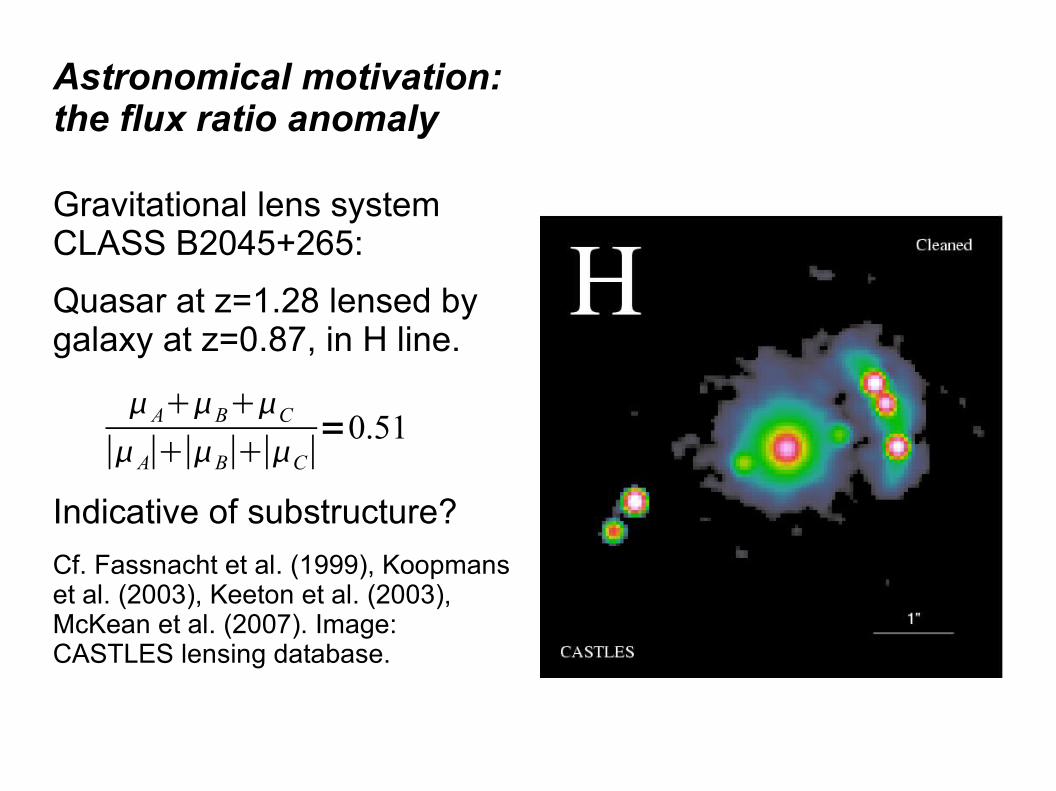
Astronomical motivation:the flux ratio anomaly

Gravitational lens system CLASS B2045+265:

Quasar at z=1.28 lensed by galaxy at z=0.87, in H line.

Indicative of substructure?

Cf. Fassnacht et al. (1999), Koopmans et al. (2003), Keeton et al. (2003), McKean et al. (2007). Image: CASTLES lensing database.

ABC

∣A∣∣B∣∣C∣=0.51

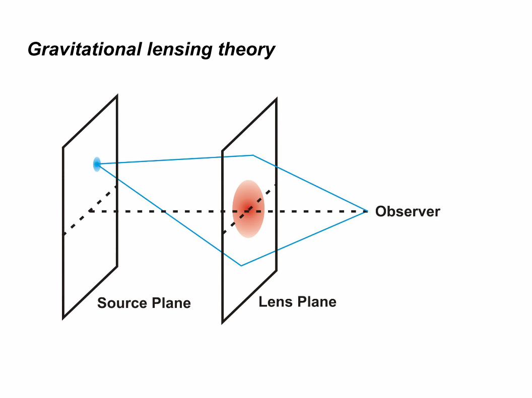
Gravitational lensing theory

Quasi-Newtonian impulse approximation: a useful framework for lensing problems in astrophysics, in the limit of

● Geometrical optics● Small deflection angles● Asymptotically Euclidean space● Thin lenses, compared to the length of the light ray

Consider the parallel lens plane and source plane containing deflecting masses and light sources,

respectively, at .

L=ℝ2

S=ℝ2

x∈L ,y∈S

Gravitational lensing theory

Gravitational lensing theory:the lensing map

Geometrical and gravitational time delay combined yields the Fermat potential given by

Then the Fermat's principle implies the lens equation

mapping images at surjectively to the source.

The lensing map is .

y x : L×S ℝ

y x =12

∣x−y∣2−x

∇ y x =0

y=x−∇ x

x

: L S ,x y

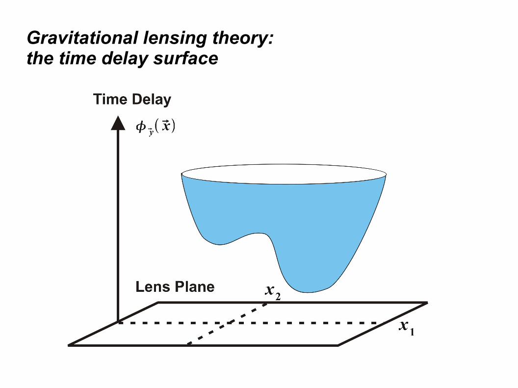
Gravitational lensing theory:the time delay surface

Gravitational lensing theory:image properties

Topology in gravitational lensing

Images are non-degenerate critical points of the Morse function , with Morse index .

Theorem [Morse, 1925]. Let be a smooth closed real manifold with dimension and Euler characteristic , and non-degenerate critical points with Morse index . Then

y x

MM d

n

∑=0

d

−1 n=M

Topology in gravitational lensing:closing the time delay surface

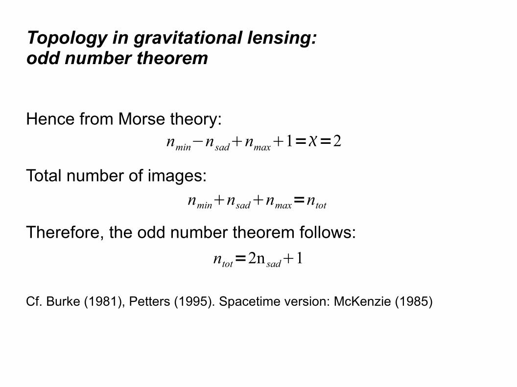
Topology in gravitational lensing: odd number theorem

Hence from Morse theory:

Total number of images:

Therefore, the odd number theorem follows:

Cf. Burke (1981), Petters (1995). Spacetime version: McKenzie (1985)

nmin−nsadnmax1==2

nminnsadnmax=ntot

ntot=2n sad1

Topology in gravitational lensing

SDSS J1004+4112. Cluster: z=0.68; quasar: z=1.73; galaxy: z=3.33.

Image: ESA, NASA, K. Sharon, E. Ofek.

Properties of image magnification

Due to Liouville's Theorem in curved spacetime, the intensity obeys

Achromaticity of gravity:

Hence flux is proportional to solid angle, and the signed image magnification is

where

The sign defines image parity.

I /3=const.

=const.

=1

det Jac Jac =

∂ y1

∂ x1

∂ y1

∂ x2

∂ y2

∂ x1

∂ y2

∂ x2

Properties of image magnification

The critical set of the lensing map is defined by in , corresponding to infinite magnification .

The critical set is mapped to caustics in by the lensing map, .

Caustics delimit domains of constant image number in .

According to singularity theory, only certain types of caustics occur generically.

L

S

Crit

Caustic =Crit

det Jac =0

S

Magnification invariants

Constant sums of signed image magnifications, independent of lens parameters and image positions.

Global magnification invariants:

● Apply to all images

● Dependent on the lens model

● Source in maximal domain

Example: for Schwarzschild and Plummer model.

Cf. Witt & Mao (1995), Dalal & Rabin (2001), Hunter & Evans (2001), Evans & Hunter (2002), Werner & Evans (2006), Werner (2007).

∑i=1

n

i=1

n

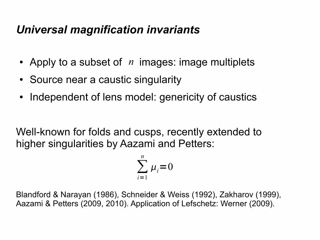
Universal magnification invariants

● Apply to a subset of images: image multiplets

● Source near a caustic singularity

● Independent of lens model: genericity of caustics

Well-known for folds and cusps, recently extended to higher singularities by Aazami and Petters:

Blandford & Narayan (1986), Schneider & Weiss (1992), Zakharov (1999), Aazami & Petters (2009, 2010). Application of Lefschetz: Werner (2009).

∑i=1

n

i=0

n

Caustic singularities: generic case

Polynomial generating potential: , with

state variables and control parameters ,

inducing a generic map and caustics as discussed above.

Stable caustics in a space of control parameters :

● Fold:

● Cusp:

where is the number of images in maximal caustic domain.

u x :ℝ2×ℝ pℝ

x= x1 , x2 u∈ℝ p , p≥2

u=y , p=2

n

n=2

n=3

x =x1 , x22

x =x1 , x1 x2x23

Caustic singularities: the cusp

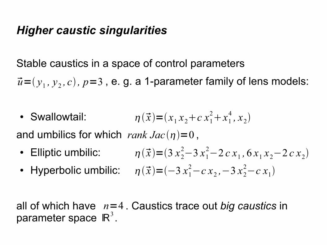
Higher caustic singularities

Stable caustics in a space of control parameters

, e. g. a 1-parameter family of lens models:

● Swallowtail:

and umbilics for which ,

● Elliptic umbilic:

● Hyperbolic umbilic:

all of which have . Caustics trace out big caustics in parameter space .

u= y1 , y2 , c , p=3

x =3 x22−3 x1

2−2 c x1 ,6 x1 x2−2 c x2

x =−3 x12−c x2 ,−3 x2

2−c x1

x =x1 x2c x12x1

4 , x2

rank Jac =0

n=4ℝ3

Singularities: big caustic of the swallowtail

Singularities: big caustic of the elliptic umbilic

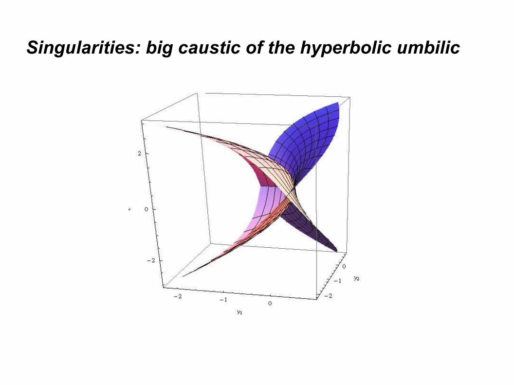
Singularities: big caustic of the hyperbolic umbilic

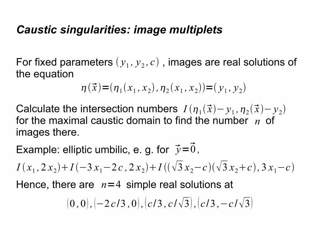
Caustic singularities: image multiplets

For fixed parameters , images are real solutions of the equation

Calculate the intersection numbers for the maximal caustic domain to find the number of images there.

Example: elliptic umbilic, e. g. for

Hence, there are simple real solutions at

y1 , y2 , c

x =1x1 , x2 ,2 x1 , x2= y1 , y2

nI 1x− y1 ,2x − y2

y=0 ,

I x1 ,2 x2 I −3 x1−2c ,2 x2 I 3 x2−c 3 x2c ,3 x1−c

n=4

0 ,0 , −2c /3 ,0 , c /3 , c /3 , c /3 ,−c /3

Solomon Lefschetz

Born 1884 in Moscow, died 1972 in Princeton, NJ.

Engineering in Paris, then emigration to USA at 21.

Turned to mathematics after accident. PhD at Clark, MA, in 1911.

A founding father of algebraic topology, in Topology (AMS, 1930).

Image: from the St. Andrews, UK, History of Mathematics Site

Lefschetz fixed point theory

Let be a closed manifold with dimension , and be differentiable. Then the fixed points of are

Intersection of graph of , , with diagonal in , :

Connection of local, geometrical properties at fixed points, the fixed point indices , with global, topological properties, the Lefschetz number , gives a Lefschetz fixed point formula:

M dim M =dff :M M

fM×M

Graph f ={x , f x ∈M×M }

Fix f ={x∈M : f x =x }

Diag M ={x , x ∈M×M }

Fix f =Graph f ∩Diag M

L

L= ∑Fix f

Lefschetz fixed point theory: real manifolds

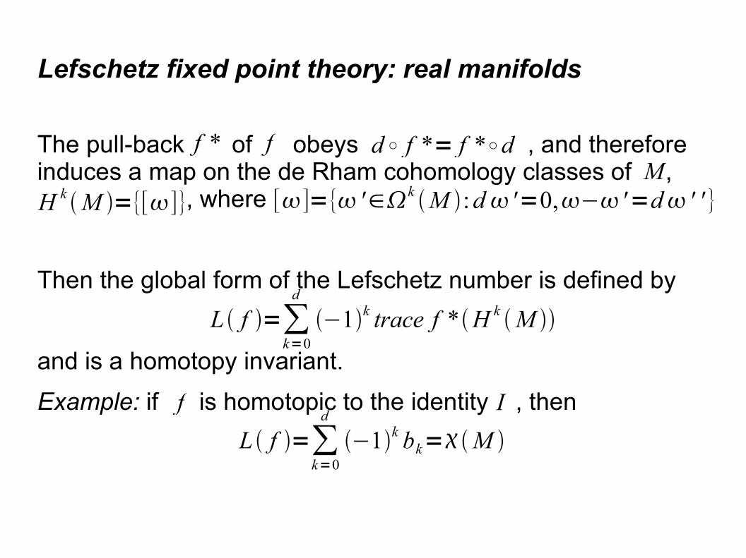
The pull-back of obeys , and therefore induces a map on the de Rham cohomology classes of , , where

Then the global form of the Lefschetz number is defined by

and is a homotopy invariant.

Example: if is homotopic to the identity , then

f * f d ° f *= f *°dM

H k M ={[]} []={ '∈k M :d '=0,− '=d ' ' }

L f =∑k=0

d

−1k trace f *H k M

f I

L f =∑k=0

d

−1k bk=M


The fixed point indices are well-defined if the intersection of with is transversal, that is, stable:

Positively oriented tangent space bases:

Left-hand side:

Rearranging,

{ e1

0 , , ed

0 , 0e1

, , 0ed }

{ e1

D f e1 , , ed

D f e1 , e1

e1 , , ed

ed}

{ e1

0 , , ed

0 , 0 I−D f e1

, , 0 I−D f ed }

T x , x M×M :

T x , x Graph f T x , x Diag M =T x , x M×M

Graph f Diag M


Hence, the local form of the Lefschetz fixed point formula:

so the fixed point indices are .

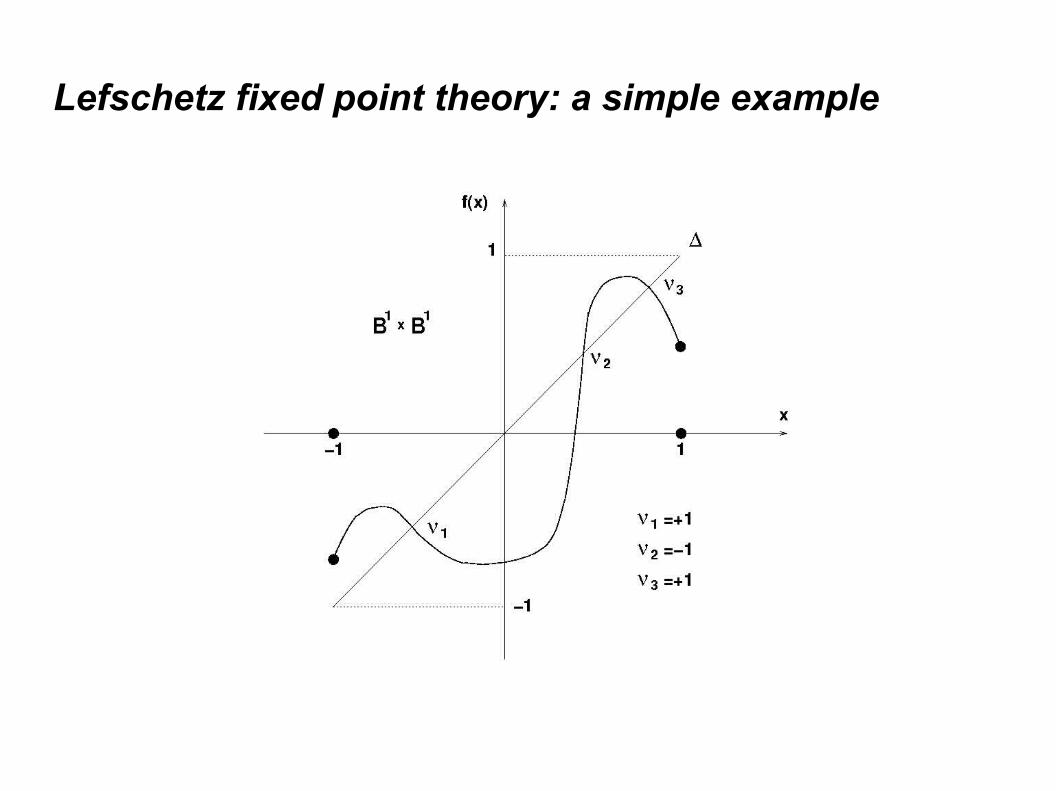
Example: map on the closed unit ball homotopic to

identity, so .

L f = ∑Fix f

sgndet I−D f

∈{−1,1}

f : B1 B1

L f =B1=1

Lefschetz fixed point theory: a simple example

Lefschetz fixed point theory: complex manifolds

Let be complex and holomorphic, that is .

Then the pull-back of obeys , and therefore induces a map on the Dolbeault cohomology classes of , , where

The holomorphic Lefschetz number is defined by

and the fixed point formula becomes

f *

f

∂° f *= f *°∂

M

H r , s M ={[]}

[]={ '∈r , sM :∂ '=0,− '=∂ ' ' , ' '∈r , s−1M }

Lhol f =∑s=0

d

−1s trace f * H 0, sM

f

∂ f =0

M

Lhol f = ∑Fix f

1det I−D f

Lefschetz fixed point theory: complex manifolds

Example: the rational fixed point theorem in complex

dynamics. For and ,

Proof: Choose local holomorphic coordinates such that

and . Then

and the result follows

using .

f ≠ IM=ℂ=ℂ∪{∞}=ℂ P1

∑Fix f

1

1−dfdz

=1=Lhol f

f 0=0 f z =dfdz

0 zO z2

12 i∮C 0

dzz− f z

=1−dfdz

0−1

12 i∮C∞ 1

z− f z −

1z dz=0

Application to gravitational lensing

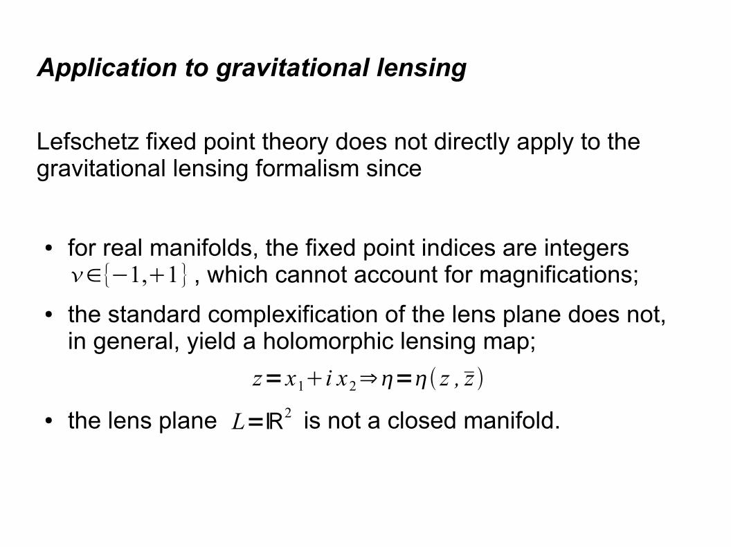
Lefschetz fixed point theory does not directly apply to the gravitational lensing formalism since

● for real manifolds, the fixed point indices are integers , which cannot account for magnifications;

● the standard complexification of the lens plane does not, in general, yield a holomorphic lensing map;

● the lens plane is not a closed manifold.

∈{−1,1}

L=ℝ2

z=x1i x2 ⇒= z ,z

Application to gravitational lensing

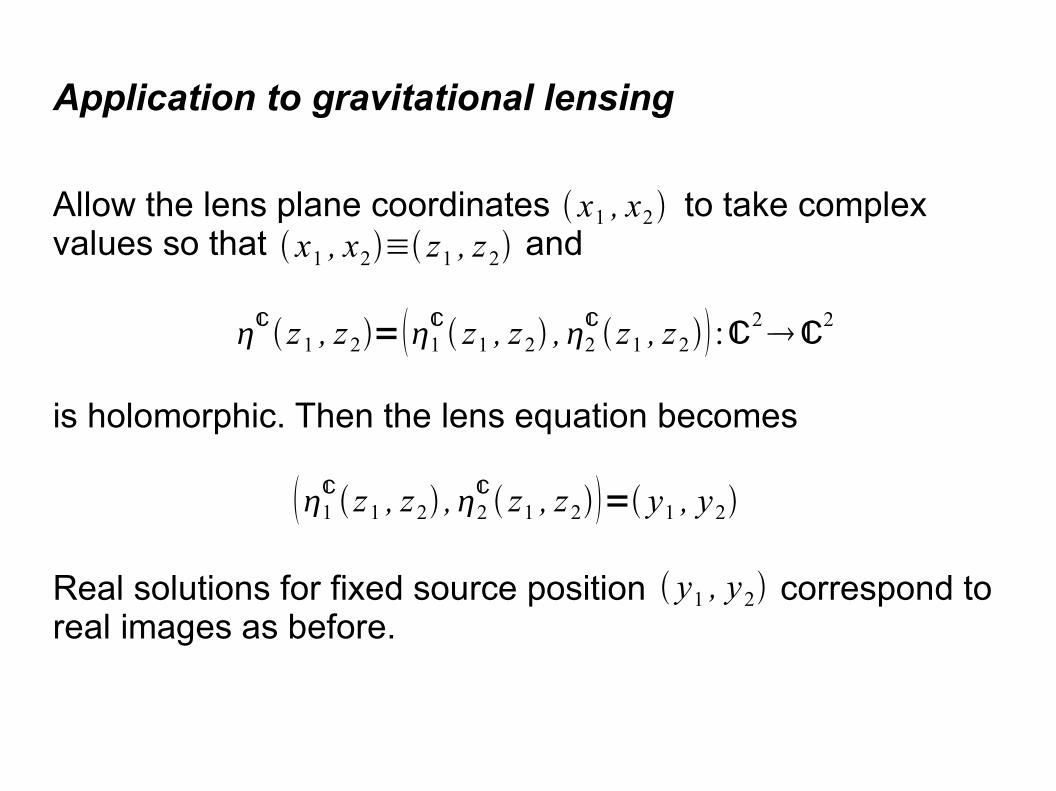
Allow the lens plane coordinates to take complex values so that and

is holomorphic. Then the lens equation becomes

Real solutions for fixed source position correspond to real images as before.

x1 , x2 x1 , x2≡ z1 , z2

ℂ z1 , z2=1

ℂ z1 , z2 ,2

ℂ z1 , z2 :ℂ2

ℂ2

1ℂ z1 , z2 ,2

ℂ z1 , z2= y1 , y2

y1 , y2

Application to generic maps of singularities

Bézout's Theorem implies

Fold Cusp Swallowtail Elliptic umbilic Hyperbolic umbilic

where are the degrees of the polynomials , respectively; the maximum number of solutions of , possibly complex; the number of real solutions in the maximal caustic domain.

deg 1ℂ deg 2

ℂ nmax n1 2 2 21 3 3 34 1 4 42 2 4 42 2 4 4

deg 1ℂ , deg 2

ℂ1

ℂ ,2ℂ nmax

1ℂ ,2

ℂ= y1, y2 n

Fixed point formalism

Construct a map such that images are fixed points,

The matrix of first partial derivatives with respect to the holomorphic coordinates is

f :ℂ2 ℂ2

f z1 , z2= z1−1ℂ z1 , z2 y1 , z1−2

ℂ z1 , z 2 y2

D f =1−∂1

ℂ

∂ z1

−∂1

ℂ

∂ z 2

−∂2

ℂ

∂ z1

1−∂2

ℂ

∂ z2


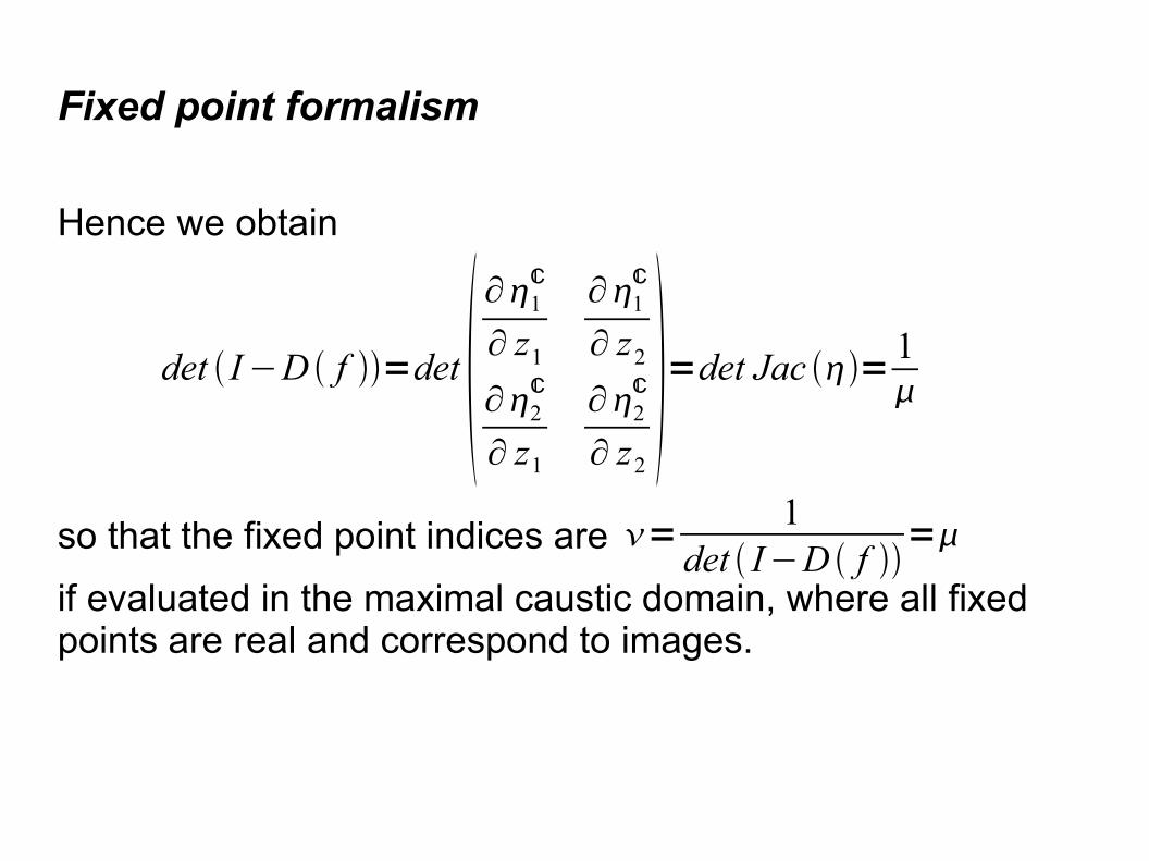
Hence we obtain

so that the fixed point indices are

if evaluated in the maximal caustic domain, where all fixed points are real and correspond to images.

det I−D f =det ∂1

ℂ

∂ z1

∂1ℂ

∂ z2

∂2ℂ

∂ z1

∂2ℂ

∂ z2

=det Jac =1

=1

det I−D f =


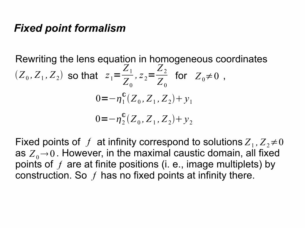
Rewriting the lens equation in homogeneous coordinates

so that for ,

Fixed points of at infinity correspond to solutions as . However, in the maximal caustic domain, all fixed points of are at finite positions (i. e., image multiplets) by construction. So has no fixed points at infinity there.

z1=Z 1

Z 0

, z 2=Z 2

Z 0

Z 0 , Z 1 , Z 2 Z 0≠0

0=−1ℂZ 0 , Z 1 , Z 2 y1

0=−2ℂZ 0 , Z 1 , Z 2 y2

f

ff

Z 1 , Z 2≠0Z 0 0


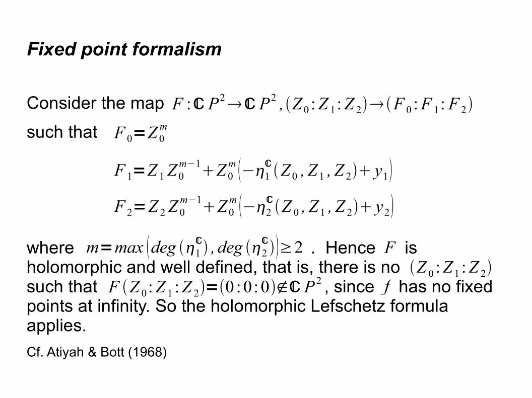
Consider the map

such that

where . Hence is holomorphic and well defined, that is, there is no such that , since has no fixed points at infinity. So the holomorphic Lefschetz formula applies.

Cf. Atiyah & Bott (1968)

F :ℂ P2 ℂ P2 ,Z 0 :Z 1:Z 2F 0 :F 1: F 2

F 0=Z 0m

F 1=Z 1Z 0m−1

Z 0m −1

ℂZ 0 , Z 1 , Z 2 y1

F 2=Z 2Z 0m−1

Z 0m −2

ℂZ 0 , Z 1 , Z 2 y2

m=max deg 1ℂ , deg 2

ℂ≥2 F

Z 0 :Z 1 :Z 2F Z 0:Z 1 :Z 2=0 : 0: 0∉ℂ P 2 f


Consider , where and .

Then on , we recover , whence

Now the non-vanishing Dolbeault cohomology classes are

if , so

since only contributes.

ℂ P2=ℂ2∪ℂP1 ℂ2 :Z 0=1 ℂ P1:Z 0=0

ℂ2 F 1= f 1 , F 2= f 2

Fix Fℂ

2=Fix f

H r , sℂP n=ℂ r=s

Lhol F =∑s=0

2

−1s trace F *H 0, s ℂ P 2=1

H 0,0 ℂ P2=ℂ

Application to universal magnification invariants

Hence,

and the result follows (Werner 2009).

1=Lhol F = ∑Fix F

1det I−D F

= ∑Fix F

ℂ2

1det I−DF

∑Fix F

ℂP1

1det I−D F

= ∑Fix f

1det I−D f

1

=∑i=1

n

i1

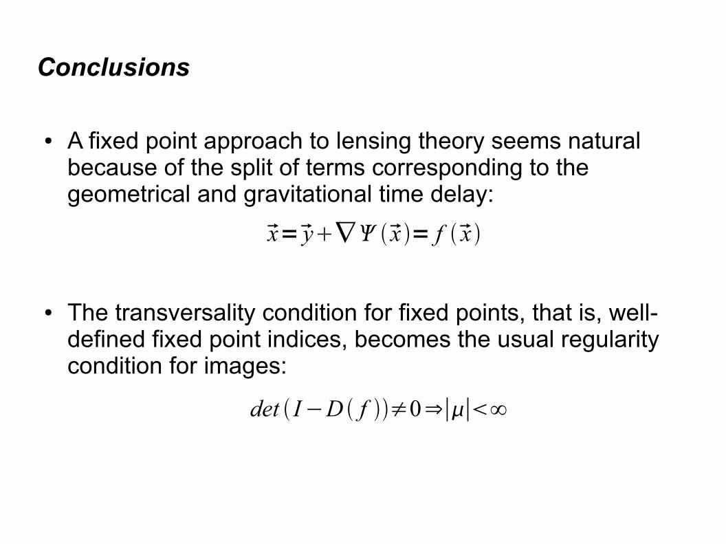
Conclusions

● A fixed point approach to lensing theory seems natural because of the split of terms corresponding to the geometrical and gravitational time delay:

● The transversality condition for fixed points, that is, well-defined fixed point indices, becomes the usual regularity condition for images:

x=y∇ x = f x

det I−D f ≠0⇒∣∣∞

Conclusions

● Lefschetz fixed point formulae are special cases of the Atiyah-Bott Theorem, which ties universal magnification invariants in with a deep result in fixed point theory and topology.

● The same formalism can be applied not only to the generic cases discussed here, but also to elliptic and hyperbolic umbilics in lensing (where there is a preferred coordinate system). Open problem: is there an extension to other magnification invariants?

● Does a spacetime version of global or universal magnification invariants exist?

Documents

Universal Magnification Invariants and Lefschetz Fixed