Embed Size (px)
Citation preview

University of New MexicoUNM Digital Repository
Physics & Astronomy ETDs Electronic Theses and Dissertations
Spring 5-13-2017
Universal Disorder in Organic SemiconductorsDue to Fluctuations in Space ChargeTZUCHENG WU
Follow this and additional works at: https://digitalrepository.unm.edu/phyc_etds
Part of the Astrophysics and Astronomy Commons, Condensed Matter Physics Commons, andthe Physical Chemistry Commons
This Dissertation is brought to you for free and open access by the Electronic Theses and Dissertations at UNM Digital Repository. It has beenaccepted for inclusion in Physics & Astronomy ETDs by an authorized administrator of UNM Digital Repository. For more information, please [email protected].
Recommended CitationWU, TZUCHENG. "Universal Disorder in Organic Semiconductors Due to Fluctuations in Space Charge." (2017).https://digitalrepository.unm.edu/phyc_etds/140

Tzu-Cheng Wu
Candidate
Physics and Astronomy
Department
This dissertation is approved, and it is acceptable in quality and form for publication: Approved
by the Dissertation Committee:
David. H. Dunlap, Chair
Vasudev M. Kenkre
Susan R. Atlas
Paul Schwoebel
John Grey

Universal Disorder in OrganicSemiconductors Due to Fluctuations in
Space Charge
by
Tzu-Cheng Wu
B.S., Tamkang University, 2008
M.S., University of New Mexico, 2013
DISSERTATION
Submitted in Partial Fulfillment of the
Requirements for the Degree of
Doctor of Philosophy
Physics
The University of New Mexico
Albuquerque, New Mexico
May, 2017
ii

c©2017, Tzu-Cheng Wu
iii

Dedication
To my mother, the greatest in the world.
iv

AcknowledgmentsI would like to thank my adviser Professor Dunlap. During my PhD journey, he wasnot only an excellent teacher, but also a wise mentor. I am grateful for his insightand guidance in this dissertation. He is the paradigm of the theoretical physicist.His ceaseless enthusiasm and creative thinking influenced the way I learned physics.Beyond the academic role, he has been an understandable family member, showingconcern for my situations during these years.
I also would like to thank Professor Kenkre. He always teaches physics with vividexpressions that are rarely found in textbooks. His distinct teaching style caused meto fall in love with Nonequilibrium Statistical Mechanics, a subject about which I hadbeen innocent for years. Listening to his anecdotes about other well-known physicistshas been exceptionally enjoyable.
Thank you Dr. Valone for introducing me to your brilliant project concerning thefragment Hamiltonian. It was the first time in my life that I became involved withreal research. Developing many different aspects of this project has been educationalfor me. I am grateful for the guidance and mentoring of Professor Atlas. Her carefulreading and inciteful commenting greatly improved this dissertation. Her remarkablecomprehensive inductive ability impresses me to no end.
I would like to thank Dr. Andrei Piryatinski and Dr. Charles Cherqui for theirmany discussions and for preliminary results that formed the basis of this work.
I am grateful to have had the support and friendship of my officemates andfellow students, Matt Chase, Karthik Chinni, Anastasia Ierides, Xiaodong Qi, SatomiSugaya, and many others in CQuiC and different groups. Special thanks go to Chih-Feng Wang, and Jui-Jen Wang, and other Taiwanese friends for their assistance.
Last but not the least, without my family’s endless support, going abroad in orderto accomplish my dream in physics would have been impossible for me. Above all, Iam grateful to my mother for staying with me for months in the final stage.
I would like to acknowledge graduate assistantship research support during theearly stages of this work from DOE/Los Alamos National Laboratory Subcontract#206753 − 1 (Dr. Steven M. Valone, Materials Science and Technology Division)to the University of New Mexico (Prof. Susan R. Atlas, Department of Physics andAstronomy).
v

Universal Disorder in OrganicSemiconductors Due to Fluctuations in
Space Charge
by
Tzu-Cheng Wu
B.S., Tamkang University, 2008
M.S., University of New Mexico, 2013
Ph.D., Physics, University of New Mexico, 2017
Abstract
vi

This thesis concerns the study of charge transport in organic semiconductors.
These materials are widely used as thin-film photoconductors in copiers and laser
printers, and for their electroluminescent properties in organic light-emitting diodes.
Much contemporary research is directed towards improving the efficiency of organic
photovoltaic devices, which is limited to a large extent by the spatial and energetic
disorder that hinders the charge mobility. One contribution to energetic disorder
arises from the strong Coulomb interactions between injected charges with one an-
other, but to date this has been largely ignored. We present a mean-field model for
the effect of mutual interactions between injected charges hopping from site to site
in an organic semiconductor. Our starting point is a modified Frohlich Hamiltonian
in which the charge is linearly coupled to the amplitudes of a wide band of disper-
sionless plasma modes having a Lorentzian distribution of frequencies. We show that
in most applications of interest the hopping rates are fast enough while the plasma
frequencies are low enough that random thermal fluctuations in the plasma density
give rise to an energetically disordered landscape that is effectively stationary for
many thousands of hops. Moreover, the distribution of site energies is Gaussian, and
the energy-energy correlation function decays inversely with distance; as such, it can
be argued that this disorder contributes to the Poole-Frenkel field dependence seen
in a wide variety of experiments. Remarkably, the energetic disorder is universal;
although it is caused by the fluctuations in the charge density, it is independent of
the charge concentration.
vii

Contents
1 Introduction 1
2 Overview of Organic Semiconductors 4
2.1 Introduction . . . . . . . . . . . . . . . . . . . . . . . . . . . . . . . . 4
2.2 Bonding . . . . . . . . . . . . . . . . . . . . . . . . . . . . . . . . . . 5
2.3 Energy Levels of Organic Molecules . . . . . . . . . . . . . . . . . . . 6
2.4 Molecular Solids and Conjugated polymers . . . . . . . . . . . . . . . 7
2.4.1 Molecular Solids . . . . . . . . . . . . . . . . . . . . . . . . . 7
2.4.2 π-conjugated Polymers . . . . . . . . . . . . . . . . . . . . . . 8
2.5 From Ordered to Disordered Organic Semiconductors . . . . . . . . . 11
2.5.1 Static Energetic Disorder . . . . . . . . . . . . . . . . . . . . . 11
2.5.2 Positional Disorder . . . . . . . . . . . . . . . . . . . . . . . . 12
2.6 Summary . . . . . . . . . . . . . . . . . . . . . . . . . . . . . . . . . 12
3 Mobility in Disordered Organic Semiconductors 14
viii

Contents
3.1 Introduction . . . . . . . . . . . . . . . . . . . . . . . . . . . . . . . . 14
3.2 Experimental Techniques . . . . . . . . . . . . . . . . . . . . . . . . . 15
3.3 Theoretical Models . . . . . . . . . . . . . . . . . . . . . . . . . . . . 18
3.3.1 Gaussian Disorder Model . . . . . . . . . . . . . . . . . . . . 19
3.3.2 Correlated Disorder Model . . . . . . . . . . . . . . . . . . . . 22
3.4 Three-Dimensional Simulations . . . . . . . . . . . . . . . . . . . . . 27
3.4.1 Remarks . . . . . . . . . . . . . . . . . . . . . . . . . . . . . . 28
3.5 Polaronic Correlated Disorder Model . . . . . . . . . . . . . . . . . . 29
3.6 Application of Disordered Organic Semiconductors . . . . . . . . . . 31
3.6.1 Organic Light Emitting Diode . . . . . . . . . . . . . . . . . . 31
3.6.2 Organic Solar Cells . . . . . . . . . . . . . . . . . . . . . . . . 32
3.7 Concluding Remarks . . . . . . . . . . . . . . . . . . . . . . . . . . . 33
4 Dielectric Friction and the Frohlich Hamiltonian 34
4.1 Motivation . . . . . . . . . . . . . . . . . . . . . . . . . . . . . . . . . 34
4.2 Mean-field Approximation . . . . . . . . . . . . . . . . . . . . . . . . 37
4.3 The Lorentz-Drude Model of a Dielectric . . . . . . . . . . . . . . . . 38
4.3.1 Example: A moving charge . . . . . . . . . . . . . . . . . . . 41
4.4 Newtonian Equation of Motion . . . . . . . . . . . . . . . . . . . . . 42
4.5 Hamiltonian Formulation of Dielectric Friction . . . . . . . . . . . . . 44
ix
Contents
4.6 Relation Between Dielectric Friction Hamiltonian and Frohlich Hamil-
tonian . . . . . . . . . . . . . . . . . . . . . . . . . . . . . . . . . . . 48
4.6.1 Canonical Transformation . . . . . . . . . . . . . . . . . . . . 50
4.6.2 Generating Function Method . . . . . . . . . . . . . . . . . . 50
4.7 Generalization of the Frohlich Hamiltonian . . . . . . . . . . . . . . . 52
4.8 Conclusion . . . . . . . . . . . . . . . . . . . . . . . . . . . . . . . . . 54
5 Charge Hopping Rate: Time Scales and Distribution of Rates 55
5.1 Introduction . . . . . . . . . . . . . . . . . . . . . . . . . . . . . . . . 55
5.2 Charge-Plasmon-Phonon Hamiltonian . . . . . . . . . . . . . . . . . . 56
5.3 Displaced Oscillator Transformation . . . . . . . . . . . . . . . . . . . 58
5.4 Time-dependent Perturbation Theory . . . . . . . . . . . . . . . . . . 60
5.5 The Ensemble Average of the Memory Function and the Hopping Rate 63
5.6 Discussions of Time Scales . . . . . . . . . . . . . . . . . . . . . . . . 64
5.6.1 The Phonon Memory Function: Cph(t, τ) . . . . . . . . . . . . 65
5.6.2 The Plasmon Part: Cpl(t, τ) . . . . . . . . . . . . . . . . . . . 67
5.7 Plasmon-Phonon-Polaron Hopping Rate . . . . . . . . . . . . . . . . 69
5.8 Summary . . . . . . . . . . . . . . . . . . . . . . . . . . . . . . . . . 69
6 Universal Spatially Correlated Gaussian Static Energetic Disorder 71
6.1 Introduction . . . . . . . . . . . . . . . . . . . . . . . . . . . . . . . . 71
6.2 Gaussian Correlated Disorder . . . . . . . . . . . . . . . . . . . . . . 72
x
Contents
6.3 Evaluation of σ and Universal Static Disorder . . . . . . . . . . . . . 74
6.3.1 Springs and Constant Force . . . . . . . . . . . . . . . . . . . 75
6.4 Universal Reorganization Energy and Universal Hopping Rate . . . . 78
6.5 One-Dimensional Mobility . . . . . . . . . . . . . . . . . . . . . . . . 78
6.6 Concluding Remarks . . . . . . . . . . . . . . . . . . . . . . . . . . . 79
7 Is Disorder Due to Plasma Fluctuations Static? 81
7.1 Introduction . . . . . . . . . . . . . . . . . . . . . . . . . . . . . . . . 81
7.2 Determination of the Static/Dynamic Cutoff Frequency ωc . . . . . . 82
7.3 Trap Concentration for Gaussian Energy Density of States . . . . . . 85
7.3.1 Uncorrelated Gaussian Disorder and Multiple Trapping Model 86
7.3.2 Correlated Disorder Case . . . . . . . . . . . . . . . . . . . . . 89
7.4 Conclusion . . . . . . . . . . . . . . . . . . . . . . . . . . . . . . . . . 91
8 Epilogue 92
Appendices 95
A Justification of Fermi’s Golden Rule 96
B Frohlich Hamiltonian 101
C Displaced Oscillator Transformation 104
xi
Contents
D The Physical Meaning of sin2(qa)/q2a2 107
References 110
xii

Chapter 1
Introduction
Organic semiconductors have been widely studied over the past five decades, at-
tracting interest not only in academic research [1–13] but also in industrial applica-
tions [14–19]. An organic semiconductor is literally a material comprised of organic
molecules or a chain of monomers exhibiting semiconducting properties. Compared
to conventional inorganic semiconductors that comprise our daily electronic devices,
they are promising because of the possibility of low-cost fabrication, realization of
large-area display devices, and flexible electronics [20]. Such applications stem from
the fundamental difference between organic semiconductors and their inorganic coun-
terparts. To achieve these realizations requires a comprehensive understanding of the
associated physics and chemistry. This dissertation focuses on electrical transport.
The underlying mechanism of how charges are transported through a material be-
gins with a microscopic description of tunneling; this shall be addressed before we
step into further detail of the transport problem involving a network of spatially
and energetically disordered hopping sites. A discussion of the motivation and the
simple model chosen for study will be made. We present new results and questions
raised from our model address possible future work. This dissertation is organized
as follows.
1
Chapter 1. Introduction
Chapter II : This chapter begins with the basics of organic semiconductors. The
bonding involved in organic molecules is concisely introduced. In order to under-
stand the band structures in a solid phase, we start from a single organic molecule
and present the concepts of molecular orbitals, energy levels, and bands. A criti-
cal factor influencing charge transport is the high degree of disorder in the organic
semiconductors. The origin of disorder is discussed.
Chapter III : Preliminary insights about charge transport are developed in this
chapter. The key quantity of interest in organic semiconductors is the mobility. This
is discussed in the context of the standard time-of-flight experiments and current-time
curves. Poole-Frenkel behavior (experimental dependence of mobility on the square
root of the field) is notably observed in a wide variety of materials. To understand
the Poole-Frenkel behavior, two theoretical models, the Gaussian disorder model
and the correlated disorder model, are introduced. Although the Gaussian disorder
model shows some consistency with experimental results in the strong field regime,
we point out its overall deficiency which supports the use of the correlated disorder
model. The correlated disorder model is also used as a rationale for understanding
the compatibility of polaronic effects in energetic disordered organic semiconductors.
Finally, we describe two selected applications of disordered organic semiconductors
− organic light emitting diodes and organic solar cells − to illustrate the importance
of charge transport.
Chapter IV : The mutual charge-charge interactions in organic semiconductors are
considerable as a result of the low dielectric permittivity. A mean field approximation
is proposed to simplify the many-body complexity and the resulting equation of
motion of a moving charge is derived. In addition, a Hamiltonian giving rise to this
underlying equation is presented. The Hamiltonian is identical to the well-known
Frohlich Hamiltonian [21,22] except for a modification to the spectral density, due to
the different choice of dielectric model. In this sense we have generalized the Frohlich
2

Chapter 1. Introduction
Hamiltonian to describe any dielectric susceptibility.
Chapter V : With the Hamiltonian in hand, standard time-dependent perturba-
tion theory is implemented to obtain the hopping rate from one molecular site to
another. Critical importance is placed on the use of Fermi’s golden rule and the
relative time scales involved in the problem. We examine the validity of the stan-
dard approach, which requires taking the ensemble average with respect to the initial
phonon state in order to evaluate the memory function. This approach fails here due
to the slow relaxation of the dielectric as compared to the hopping rate.
Chapter VI : A significant achievement of the mean-field solution is that it pro-
vides a picture that the local fluctuations of the charge density give rise to static
disorder that is spatially correlated and independent of the concentration of charges.
The magnitude of the site energy fluctuation is large enough to be significant at room
temperature and the site energy correlation is the same as for the charge-dipole in-
teraction in the correlated disorder model.
Chapter VII : A self-consistent equation to determine the magnitude of static
disorder is derived. It is found that universal static disorder is induced by mutual
charge interactions at room temperature for sufficiently low charge concentration.
Chapter VIII : In the last chapter of this dissertation, we summarize our results
and address the limitations of our model and directions for improvement.
3

Chapter 2
Overview of Organic
Semiconductors
2.1 Introduction
We begin by reviewing some essential concepts concerning organic semiconductors.
Organic molecules are composed of carbon atoms in which four valence electrons
in each carbon play the role of bonding, such as the formation of single, double,
and triple bonds linking neighboring molecules. In the beginning of this chapter,
a concise introduction to bonding is presented. Next, molecular energy levels for a
simple organic molecule are addressed to introduce the concepts of molecular orbitals
and the band gap in solids. This is followed by a discussion of how an ensemble
of molecules or a chain of monomers in the solid phase form a semiconductor. A
significant factor impacting the efficiency of charge transport is the periodicity of
the material. Noncrystalline structures contain ubiquitous positional and energetic
disorder. The effects of disorder will be discussed at the end of the chapter.
4

Chapter 2. Overview of Organic Semiconductors
(a) Ethane: C2H6 (b) Ethylene: C2H4 (c) Acetylene: C2H2
Figure 2.1: Examples of single bonds, double bonds, and triple bonds in organicmolecules.
2.2 Bonding
The fundamental element in organic molecules is the carbon atom, consisting of
six electrons with a ground state electron configuration 1s22s22p2. The outer four
valence electrons residing in the 2s and 2p orbitals participate in bonding. In general,
a carbon may be involved with three types of bonds, single, double, and triple,
which can be understood by the hybridization of atomic orbitals [23]. Consider
ethane (C2H6) containing only single bonds as an example. For each carbon, three
of the four valence electrons form C-H covalent bonds with hydrogen, respectively,
and the remaining valence electron couple with the other electron provided by the
other carbon via a C-C covalent bond (see Figure 2.1a.) The single bond is also
referred to as a σ bond. The standard mechanism behind the formation of bonding
arises from reduction in energy facilitated by the overlap of the atomic orbitals.
The bond between hydrogen and carbon is an overlap between a hydrogen s-orbital
and a carbon sp3-orbital. The C-C bond is the overlap between two sp3 carbon
orbitals provided by each carbon. σ-electrons are often treated as localized, hardly
participating in physical processes. In addition to the σ bond, different hybridizations
of carbon orbitals show different structures such as in the example of ethylene (C2H4)
drawn in Figure 2.1b. Each carbon consists of three sp2-orbitals forming two σ bonds
with the hydrogens, and one σ bond with the other carbon. The remaining two pz
5

Chapter 2. Overview of Organic Semiconductors
(a) Bezene: C6H6(b) Energy levels of benzene
Figure 2.2: Benzene structure and energy levels.
orbitals from the two carbons overlap to form a covalent bond perpendicular to the
molecular plane of the σ bonds. This is called a π-bond and constitute the C=C
double bond. The orbitals in a π-bond have less overlap than the orbitals in σ bonds,
and the π-electrons are delocalized. They play a key role in electrical transport and
optical excitations. The last configuration shown in Figure 2.1c is acetylene (C2H2).
Each carbon provides two sp-orbitals to form two σ bonds; one is to a hydrogen and
one is to the other carbon. The rest of the carbon 2p-orbitals form two π bonds
perpendicular to the molecular axis, constituting a C≡C triple bond.
2.3 Energy Levels of Organic Molecules
The semiconducting properties of organic molecules depend on the energy levels.
A paradigm for this discussion is benzene (C6H6), which is the simplest aromatic
hydrocarbon, sketched in Figure 2.2a. Of the 24 valence electrons in the six carbons,
six form σ bonds with hydrogens, twelve form σ bonds between carbons, and the
six remaining electrons are in the pz orbitals. Only π-electrons account for the
excitations of benzene. If isolated carbons are considered, the six pz orbitals of the
six carbons are degenerate. Due to the mutual interactions between adjacent carbons,
6

Chapter 2. Overview of Organic Semiconductors
the degeneracy is broken, exhibiting a split of the energy levels that is schematically
drawn in Figure 2.2b. The corresponding eigenfunctions |ψn〉 are linear combinations
of atomic (pz) orbitals |ϕi〉 with coefficients ci, namely
|ψn〉 =∑
i=a,b,···
ci|ϕi〉, (2.1)
where n = 1, 2, · · · , 6. The |ψn〉 orbitals are called molecular orbitals. They are
delocalized. (We will not address explicit calculations of energy splittings using the
tight-binding Huckel model [23].) Each eigenstate can be occupied by two electrons
with opposite spins according to the Pauli exclusion principle, so that the ground
state consists of the lower three levels fully occupied by six electrons. The upper
three levels are empty. The energy difference between the highest occupied molecular
orbital (HOMO) and the lowest unoccupied molecular orbital (LUMO) is known as
a HOMO-LUMO gap, Eg, and is analogous to the band gap in a semiconductor.
2.4 Molecular Solids and Conjugated polymers
Bonding is more interesting when many small molecules come together to form a
crystal or a polymer chain. In this section we discuss some of the basics concerning
molecular solids and polymers.
2.4.1 Molecular Solids
In solids, bonds between atoms and molecules are described as being of the covalent,
metallic, ionic, and van der Waals types. Traditional inorganic semiconductors (e.g.
Si, Ge, and GaAs) are formed via covalent bonds. In organic solids, the van der
Waals bond is predominant; although the building-block molecules are neutral and
nonpolar, a fluctuating molecular dipole moment generates a dipolar field, attracting
7

Chapter 2. Overview of Organic Semiconductors
(a) Naphthalene: C10H8
(b) Unit cell in a monoclinic structure ofnaphthalene crystal. The unit cell con-sists of two naphthalene molecules speci-fied by lattice vectors a, b, and c respec-tively. Figure reproduced from [24].
Figure 2.3: Van der Waal crystal for naphthalene
the fluctuating dipole moments of the surrounding molecules. This force between
molecules is proportional to 1/R6, where R is the separation distance two molecules.
It is definitely a weak, long-range interaction as compared to the Coulombic forces
comprising a covalent bond. Figure 2.3 shows the unit cell of a typical van der
Waals crystal; naphthalene (C10H8), packed in a herringbone structure. The energy
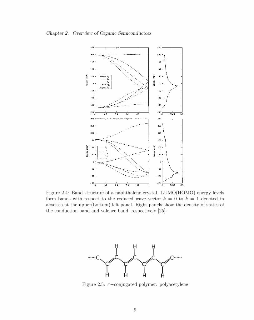
levels of the periodic structure form bonds, shown in Figure 2.4. Organic crystals
are semiconductors due to the fully occupied lower bands (valence band) below the
Fermi level, and the fully empty upper bands (conduction band) above the Fermi
level.
2.4.2 π-conjugated Polymers
A long π-conjugated polymer is a semiconductor. A polymer, by definition, is made
of repeated units of monomers. For example, polyacetylene, drawn in Figure 2.5, is
composed of a chain of monomers (C2H2). When two monomers get close, a strong
covalent σ bond between carbons forms a dimer. This process is repeated to make
the overall length of monomers grow; typically the number of repeated units is over
8
Chapter 2. Overview of Organic Semiconductors
Figure 2.4: Band structure of a naphthalene crystal. LUMO(HOMO) energy levelsform bands with respect to the reduced wave vector k = 0 to k = 1 denoted inabscissa at the upper(bottom) left panel. Right panels show the density of states ofthe conduction band and valence band, respectively [25].
Figure 2.5: π−conjugated polymer: polyacetylene
9

Chapter 2. Overview of Organic Semiconductors
(a) Without Peierl’s instability. (b) With Peierl’s instability.
Figure 2.6: Band structure of half-filled π-conjugated polymers before and afterdimerization. The reciprocal lattice vector k is represented in a reduced Brillouinzone.
a hundred. In a pristine polymer strand, there is an alternating pattern of single-
double bonds. This is called the π-conjugated configuration. The energy spectrum
can be understood with the tight-binding model. Suppose a certain polymer has N
sites (monomers) in which there are N π-electrons. A single energy band allows,
in principle, 2N electrons to fill in the N energy states. One would think that
it should be a conductor since the energy band is half-filled, but it turns out to
be a semiconductor. The reason is that a double bond is shorter than a single
bond because of stronger interactions. Consequently, having equal bond lengths is
an unstable configuration. It can be shown that adjusting the bond lengths by δ
alternatively, a− δ for a double bond and a+ δ for a single bond, gives a lower free
energy. This dimmerization effect is known as the Peierl’s instability [26–28], and it
opens an energy gap at the Fermi level, as shown in Figures 2.6a and 2.6b. It is for
this reason that half-filled polymer strands show a semiconducting property.
10

Chapter 2. Overview of Organic Semiconductors
2.5 From Ordered to Disordered Organic Semi-
conductors
The molecular solids or conjugated polymers we have discussed so far are periodic
structures for which energies form bands. However, it is inevitable that a system
will contain impurities, structural defects, or be of a polycrystalline or glass nature,
destroying the ordered single crystals [1, 29]. This is referred to as static disorder.
In addition, the periodicity will be perturbed by vibrations of the lattices. This is
referred to as dynamic disorder. Both serve to scatter a Bloch state, reducing its mean
free-path. While such scattering is considered a small perturbation in metals and
inorganic semiconductors, in the case of organic van der Waals solids, the bandwidths
are narrow to begin with, and scattering can easily reduce the mean free-path so that
it is comparable to the lattice constant [30]. In such case, a description of charge
transport is most accurately formulated as a perturbation in site space: free charges
spend most of their time sitting on molecules at particular locations in space and
occasionally tunnel to adjacent molecules (if they are unoccupied). This is referred
to as hopping conduction.
Static disorder further limits the hopping conductivity in two ways. When site
energies vary from one location to the next, charge can become trapped in regimes
of low energy. Static energetic disorder has been called diagonal disorder by Bassler
et al. [1, 2, 6, 31, 32]. Disparity in tunneling distances due to variations in molecular
density has been called off-diagonal disorder by Bassler et al. [1, 2, 6, 31,32].
2.5.1 Static Energetic Disorder
The phrase site energy refers to the HOMO energy level if the injecting charge is
a hole, or to the LUMO energy level if it is an electron. A straightforward mecha-
11

Chapter 2. Overview of Organic Semiconductors
nism for static disorder can be understood by considering the example of molecularly
doped polymers, where an amorphous structure is doped with small molecules that
distribute themselves randomly in space. Often these dopant molecules have per-
manent dipole moments forming a disordered dipolar field. When we introduce an
electron or hole into this field, its energy depends on the arrangement of permanent
dipole moments located at surrounding molecules. There exist other mechanisms for
site-energy variations which are extensively discussed by Schein et al. [31]. For the
case of conjugated polymers, a linear chain can be twisted or bent in an irregular
form. Such structural disorder causes the overall conjugation length to be cleaved
into segments with smaller conjugation lengths. Each segment can be assigned a site
energy, depending on its length.
2.5.2 Positional Disorder
Positional disorder describes spatial variations between molecules in an amorphous
solid or in solution-processed polymers. It is evident that the inter-site distance is
not a fixed constant, leading to a variation of the tunneling matrix element between
sites.
2.6 Summary
We have presented many concepts for the purpose of understanding charge trans-
port in organic semiconductors. In the presence of large disorder, band (coherent)
transport is suppressed, and electrons or holes undergo (incoherent) hopping between
adjacent LUMO or HOMO levels, respectively. The critical physical observable that
characterizes charge transport is the mobility. In the next chapter, we provide an
overview of fundamental mobility measurements and contemporary theoretical mod-
12

Chapter 2. Overview of Organic Semiconductors
els to interpret the observed results.
13

Chapter 3
Mobility in Disordered Organic
Semiconductors
3.1 Introduction
For the sake of properly analyzing charge transport in disordered organic semicon-
ductors, all relevant factors, such as the morphology of the disorder, the spatial
configuration of the site energies, the number of total charges, and the distributions
of charges must be considered. Developing a unified theory is very challenging due to
the problem’s notorious complexity. Instead of tackling the problem in its entirety,
reduced models are often developed to predict experimental results. One remarkable
behavior observed in time-of-flight experiments for many organic semiconductors is
the Poole-Frenkel law, i.e., that the logarithm of the mobility µ is proportional to
the square root of the external electric field E. With this in mind, we begin with
a discussion of the time-of-flight experiments that determine the mobility. On the
theoretical side, two of the best known models are the Gaussian disorder model [33]
and the correlated disorder model [34], and both have been used to understand ob-
14

Chapter 3. Mobility in Disordered Organic Semiconductors
Figure 3.1: Schematic of time-of-flight experiment. Charges formed by dissociatedelectron-hole pairs migrate in the external field E generating current I in the externalcircuit.
served experimental data. These two models will be discussed in detail as required
preliminary knowledge. Moreover, a long-standing dilemma of including the pola-
ronic effect [35, 36] with static disorder is resolved by using the correlated disorder
model [37]. Finally, we discuss two emerging commercial applications of disordered
organic semiconductors: organic light emitting diodes and organic solar cells.
3.2 Experimental Techniques
Use of the time-of-flight technique to measure the mobility of photo-injected charges
in organic semiconductors began in the early 60′s with experiments by Kepler [38]
and LeBlanc [39]. The schematic setup for a time-of-flight experiment is illustrated
in Figure 3.1. The sample is a parallel plate capacitor filled with the organic semi-
conductor of interest. A short laser pulse penetrates through one semitransparent
electrode, creating excitations at one end of the sample. In the presence of an exter-
nal electric field E, the narrow (compared to the thickness of the organic semicon-
ductor) excitation sheet is decomposed into free electrons and holes; under forward
bias, electrons reside at the adjacent electrode, while holes drift to the other end of
15

Chapter 3. Mobility in Disordered Organic Semiconductors
(a) Gaussian transport in the ab-sence of deep traps [1, 2].
(b) Dispersive transport induced bydistributed deep traps [1, 2].
the electrode generating a current I. A photocurrent has a classical profile shown
in Figure 3.2a. Apart from a peak near t = 0, the current-time transient shows a
plateau with constant value, followed by a tail signifying the arrival of the charge
sheet at the other side of the sample [1,2]. The transit time τ is defined by the width
of the plateau, and indicates the time for the charge sheet to cross the sample. It
follows that the drift velocity is v = L/τ , where L is the thickness of the sample.
For normal diffusive transport, the carrier packet assumes the shape of a drifting
Gaussian with width scaling as√t and mean scaling as t, leading to a narrow tail
width as compared to the plateau width as E is increased. In the case of a strongly
disordered or amorphous sample, what is observed is a vanishing plateau, blending
together with the tail in a universal profile that is independent of E, as shown in Fig-
ure 3.2b. This is referred to as dispersive transport. It arises when the trap-release
time is comparable to the time of flight. Without a flat plateau and sharp decay in
time, the way to determine the transient time τ is to observe the significant change
in the slope on a double logarithmic plot. Readers who would like to know how to
interpret dispersive transport may refer to the standard multiple trapping model and
the Scher-Montroll theory [40] and associated work [1, 2, 41].
Given the transit time, the time-of-flight mobility is determined by
µ =v
E=L2
τV, (3.1)
16

Chapter 3. Mobility in Disordered Organic Semiconductors
Figure 3.3: The characteristic hole mobility of TPM doped PS has E1/2 dependence.Figure reproduced from reference [49].
where V and E = V/L are the applied potential and field, respectively. In the
early 1970′s, Pai [42] and Gill [43] performed time-of-flight experiments on poly
(N-vinylcarbazole) (PVK) to measure its mobility. An empirical expression for the
mobility was proposed:
µ = µ0e− ∆kT e
B√E(
1kT− 1kT0
), (3.2)
where ∆ is an activation energy, B is the Poole-Frenkel factor, and T0 is known as
Gill’s compensation temperature. Both T0 and ∆ are inter-site distance dependent
quantities. Since then, the time-of-flight technique has been applied to many differ-
ent organic semiconductors in order to obtain their mobilities [2,44–48]. For instance,
Figure 3.3 shows the hole mobility with respect to different temperatures measured
for poly(styrene) (PS) doped with triphenylmethane (TPM) [49]. It was concluded
that disordered organic semiconductors often show a universal Poole-Frenkel behav-
ior,
lnµ ∼√E,
17

Chapter 3. Mobility in Disordered Organic Semiconductors
for a wide range of field strengths from 104 ∼ 106 V/cm. However, an underlying
theoretical model to explain the Poole-Frenkel law was not developed until the 90′s.
3.3 Theoretical Models
In time-of-flight experiments, one often works with sufficiently low injection so that
charge-charge interactions can be ignored. In that case the characteristics of a drift-
ing of sheet of charge can be determined by looking at the distribution of possible
outcomes for a single charge whose evolution from site to site is described by the
master equation,
dPmdt
= Rm+1,mPm+1 +Rm−1,mPm−1 − (Rm,m−1 +Rm,m+1)Pm. (3.3)
Here Pm is the probability to find the charge on the site labeled by the integer m,
and Rm±1,m denotes the hopping rate from site m± 1 to site m. Eq. (3.3) describes
evolution on a one-dimensional chain of sites with nearest-neighbor connections, but
it is straightforward to extend this to higher dimensions by replacing m with a vec-
tor m, and to include more than nearest-neighbor transitions. Due to randomly
distributed site energies, it is not feasible to find an analytical solution in general.
Monte Carlo simulations have been employed extensively to solve this master equa-
tion in order to fit experimental results with empirical parameters [33, 34, 37, 50].
These simulations led to significant insights for understanding the role of micro-
scopic mechanisms involved in interpretation of data. For instance, the underlying
mechanism of the Poole-Frenkel law (lnµ ∼√E) observed in various experiments
was a lasting mystery in the community for 25 years, until Garstein and Conwell [51]
examined the effect of spatially correlated disorder using Monte Carlo simulations.
Another remarkable feature is that disorder-controlled transport with a Gaussian
density of states displays a 1/T 2 dependence for the mobility, which differs from the
Arrhenius 1/T dependence. Nevertheless, it is sometimes difficult to determine the
18

Chapter 3. Mobility in Disordered Organic Semiconductors
exact T-dependence from experimental data due to the limited temperature range.
This temperature dependence is related to the critical question of whether the ther-
mal activation is dominated by the effect of static disorder or the effect of dynamic
disorder (polaron), since for the latter the characteristic temperature dependence is
1/T .
Two predominant energetic disorder models generally used in the literature, the
Gaussian disorder model [33] and the correlated disorder model [34] are addressed
in this section. Several different analytical approaches for understanding charge
transport in disordered systems include (1) variable range hopping [52], (2) percola-
tion [53–56], and (3) the multiple trapping model [57]. Some review articles [58–60]
and monographs [61,62] are provided.
3.3.1 Gaussian Disorder Model
The essence of the Gaussian disorder model is the well-known central limit theorem
of probability theory. Consider a molecularly doped polymer in which each molecular
site interacts with many surrounding polarizable entities [63–67]. According to the
central limit theorem, as the number of independent interactions increases, the site
energy distribution approaches a Gaussian,
g(u) =1√2πσ
e−u2/2σ2
, (3.4)
characterized by the variance σ. The Gaussian disorder model provides a guideline
for assigning site energies randomly from the density of states g(u), as illustrated in
Figure 3.4. It allows us to understand that charge carriers hop “up” and “down” en-
ergetically while traversing a sample. Bassler [33,68] pursued this idea while solving
the master equation with a Monte Carlo simulation. For simplicity, Bassler chose to
use a Miller-Abrahams-type hopping rate [69] to specify charge hopping from site i
19

Chapter 3. Mobility in Disordered Organic Semiconductors
Figure 3.4: Uncorrelated site energy distribution for a Gauusian density of states.
to site j:
Rij = R0e−αrij
1, if u(rj) ≤ u(ri)
e−|u(rj)−u(ri)|/kT , if u(rj) > u(ri)
. (3.5)
Here R0 is called the attempt frequency, rij = |ri − rj| is an inter-site distance, and
kT is the thermal energy. The localization length 1/α characterizes the extent of the
localized molecular wavefunction. He introduced an expression for the mobility
µ = µ0
e−
49
σ2
k2T2 e2.9×10−4
(σ2
k2T2−Σ2)√
E, for Σ ≥ 1.5
e−49
σ2
k2T2 e2.9×10−4
(σ2
k2T2−2.25)√
E, for Σ ≤ 1.5
. (3.6)
where Σ denotes the degree of positional disorder. This expression was a phenomeno-
logical parametrization of the numerical results obtained for numerous simulations.
Bassler’s simulations actually showed exponential dependence of mobility with field,
but not agreement with the Poole-Frenkel law, and his parametrization of√E was an
approximation to E. The 1/T 2 temperature dependence in the prefactor is expected
for Gaussian density of states. Bassler provided an explanation for equilibration in
which a charge is to be imagined initially sitting on a site whose energy is chosen
randomly from the Gaussian density of states. After experiencing a series of uphill
and downhill hops, the charge will relax to an energy level determined by
u∞ ≡∫∞−∞ ug(u)e−u/kT∫∞−∞ g(u)e−u/kT
= − σ2
kT. (3.7)
20

Chapter 3. Mobility in Disordered Organic Semiconductors
Figure 3.5: Temporal evolution of a charge carrier approaching equilibration. Figurefrom Bassler’s simulation [33].
The temporal evolution of the spread of the energy distribution of charges as found
in Bassler’s simulation is shown in Figure 3.5. After equilibration, a charge under-
goes thermally-activated uphill hops to reach the transport energy [33] which plays
the role of a mobility edge in disordered systems [70, 71]. Consequently, one ex-
pects a thermally-activated hopping rate to overcome a potential barrier ∆, with the
limiting-rate hop taking the form
R = Rce−β∆ = Rce
−C( σkT
)2
, (3.8)
where Rc is a barrier-free transition rate, and C is a scaling parameter, found to be
about 4/9 in 3D simulations. Taking advantage of the Einstein relation µ = eD/kT ,
one expects the mobility to be of the form
µ =eD
kT=ea2
kTR ∼ e−C( σ
kT)2
, (3.9)
where D is the diffusion constant and a is an average inter-site distance. The reason
the Arrhenius law fails is because the charge resides predominantly in a tail state of
the quickly decaying Gaussian distribution.
It turns out that the critical flaw in Bassler’s work that prevented an under-
standing of the Poole-Frenkel law was the assumption, made for simplicity, that
21

Chapter 3. Mobility in Disordered Organic Semiconductors
site energies are independent. In a real system, the surrounding entities (polariz-
able molecules, or permanent dipoles) that affect the energy of one hopping site
also affect the energies of its neighbors, leading to a spatially correlated landscape.
Gartstein and Conwell [51] showed that correlations distribute the field dependence
of the mobility over a wider range resembling√E. Subsequently Dunlap, Parris,
and Kenkre [34] showed analytically that the algebraic decay of the energy-energy
correlation function for the charge-dipole interaction gives the Poole-Frenkel law for
sufficiently large disorder.
3.3.2 Correlated Disorder Model
Consider the following scenario to develop a physical picture of correlated site en-
ergies. We have discussed how the charge-dipole interactions in molecular doped
polymers describe a moving carrier on one site i interacting with permanent dipoles
at surrounding dopants. Since these permanent dipoles are temporally fixed, they
provide a static dipolar field. Placing a charge in this field requires an energy u(ri).
One would not expect that an adjacent site energy would fluctuate from u(ri) sub-
stantially. It follows that site energies are mutually correlated in some manner and
not independent random variables. This picture is the essence of the correlated disor-
der model. Thus, we expect the site energies build up an energy landscape illustrated
in Figure 3.6. The resulting site energy correlation function [72] for the charge-dipole
interaction can be shown to be
〈u(ri)u(rj)〉 = σ2 a
rij(3.10)
Here σ is standard deviation of the Gaussian introduced earlier, and a is defined
as the site-radius. The algebraic 1/rij decay of the correlation function reflects the
charge-dipole interaction.
The one dimension analytical result of Dunlap, Parris, and Kenkre [34] utilized
22

Chapter 3. Mobility in Disordered Organic Semiconductors
Figure 3.6: Correlated site energy distribution for a Gauusian density of states.
the Derrida [73] technique with a simplified hopping rate having symmetric detailed
balance,
Ri,i±1 = R0e−1
2β(ui±1−ui∓eEρ).
denoting a hopping rate from site i to site i ± 1 separated by an inter-site distance
ρ = 2a. For a chain of N sites with periodic boundary conditions, the mobility is
given by
µ =ρ/E∑N
n=1 e−β(n−1)eEρ〈eβ(un−u1)R−1
n,n+1〉
≈ µ0
βeE∫∞
0dye−βeEy〈e−βu(0)eβu(y)〉
. (3.11)
Here µ0 = βR0eρ2. The approximation of the sum over n by an integral in the
second line relies on the energy eEρ being small compared to kT and that the long-
range part of the energy-energy correlation function is slowly (algebraically) varying
with site separation. Since u(y) is a Gaussian random variable, the configurational
average is of the form
〈e−β(u(0)−u(y))〉 = e12β2〈(u(0)−u(y))2〉 = e−β
2σ2
eβ2σ2 a
y .
Omitting prefactors, the integral determining the mobility is of the form∫ ∞0
dye−βeEye−β2σ2 a
y .
23

Chapter 3. Mobility in Disordered Organic Semiconductors
Although this integral has an exact solution associated with the modified Bessel
function of the third kind K1(x), it is more intuitive to implement a saddle point
approximation to obtain an asymptotic result for large disorder. We will discuss
the physical meaning of saddle point later on. Let us define the exponent f(y) ≡
−βeEy − β2σ2a/y. The extreme value is located at df/dy|y0 = 0, which vanishes
inversely with the square root of the electric field,
y0 =βσ√a√
βeE. (3.12)
This extreme point is a maximum. The essence of the saddle point approximation is
that the main contribution of the whole integral is determined by the vicinity of y0,
and this is the case for a strongly disordered system, i.e. for β2σ2 1. We expand
f(y) ≈ f(y0) + f ′′(y0)(y − y0)2/2 around y0, and Eq. (3.12) reduces to a Gaussian
integral,∫ ∞−∞
dxef(y0)e−f′′(y0)x
2
2 = ef(y0)
√2π
f ′′(y0)=
√πβσ(a)1/4
(βσE)3/4e−2βσ
√βeEa (3.13)
where x = y − y0. With this result, the mobility is found to be of the Poole-Frenkel
form
µ = µ0(E) e−β2σ2
e2βσ√βeEa, (3.14)
where the prefactor,
µ0(E) = µ0
√πβσ
√βeEa,
depends algebraically (non-exponentially) on E. It is evident that both the Poole-
Frenkel law lnµ ∼√E and a Gaussian-controlled prefactor lnµ ∼ 1/T 2 are obtained.
This mobility expression covers a wide range of electric fields from 8× 10³ V/cm to
2 × 10⁶ V/cm, consistent with experimental results as shown in Figure 3.7 [47].
New physical insight concerning length scales is needed to understand the correlated
disorder model [74]. In the Gaussian disorder model, the inter-site distance is the
24

Chapter 3. Mobility in Disordered Organic Semiconductors
Figure 3.7: Prediction of Poole-Frenkel law according the dipolar-disorder modelfor DEG-doped polycarbonate. The fit parameters can be found in the originalreferences [34,47]. Figure reproduced from reference [34]
only length scale that enters in the formulation. Yet this is not so for correlated
disorder. We can see in the sketch from Figure 3.8 that a proper length scale for
describing the transport is the size of the energetic valley measured from the bottom
to the rim. In the presence of an external field, it is evident that a deep and wide
energetic trap is sufficiently tilted to lower its barrier height by an amount eEr at
the rim, where r is the distance between the bottom and the rim. The time spent
for a charge escaping from a tilted trap is lowered by a reduction factor e−eEr/kT as a
Figure 3.8: An energy valley formed by correlated site energies denoted by ε. Withthe aid of the electric field, the size of of the rate-limiting trap decreased. Sketchedand in [74].
25

Chapter 3. Mobility in Disordered Organic Semiconductors
result. The meaning of the saddle point approximation is that the overall transport
time is determined by the time to escape from rate-limiting critical traps with size rc
whose escape height is reduced by the field e−eErc/kT [74]. The average escape time
from a trap with size r is
〈τ(r)〉 = τ0〈e((u(r)−u(0))−eEr)/kT 〉 (3.15)
= τ0e−eEr/kT e(σ/kT )2(1−a/r), (3.16)
where τ0 is the characteristic trap-free escape time. The critical size is the one for
which the derivation of the exponent vanishes,
d
dr
[−eErkT
+( σ
kT
)2 (1− a
r
)] ∣∣∣∣∣rc
= −eEkT
+( σ
kT
)2 a
r2
∣∣∣∣∣rc
= 0.
Solving for r = rc we find
rc =βσ√a√
βeE. (3.17)
Substituting into Eq. (3.16), we find the critical escape time to be
〈τ(rc)〉 = τ0e(β2σ2−2βσ
√eEa), (3.18)
from which it follows for trap-limited mobility
µ ∝ 1
〈τ〉=
1
τ0
e−β2σ2
e2βσ√eEa, (3.19)
where τ0 is the trap-free transit time. This is consistent with what we derived in Eq.
(3.14), and rc is exactly the same as yc for the saddle point approximation. This is
not surprising since the sequential nature of transport in one-dimension leads to the
same average of times that arises in trap-limited conductivity in general.
As a final remark, we point out why the (uncorrelated) Gaussian disorder model
fails to describe the Poole-Frenkel field dependence. For large enough disorder, the
rate-limiting step for transport is determined by the time for a charge to climb out
26

Chapter 3. Mobility in Disordered Organic Semiconductors
of a low-energy site, a trap. The electric field lowers the activation barrier by the
Boltzmann factor e−βeEr, but for a landscape in which site-energies are assigned at
random, r is on the order of a lattice constant, giving a field-dependent mobility
increasing as eβeEa. Thus, the mobility increases exponentially with E, and not√E.
Indeed, this linear behavior with E has been shown in Monte Carlo simulations with
the Gaussian disorder model [75], and it should have put the matter to rest.
3.4 Three-Dimensional Simulations
In the same (1995) year that Garstein and Conwell [51] showed the importance of
spatially-correlated energetic disorder, Novikov and Vannikov [72] performed a simu-
lations showing how randomly oriented permanent dipoles create a correlated energy
landscape, with energy-energy correlation function 〈u(r)u(0)〉 ∼ 1/r decaying slowly,
algebraically, with separation. They produced an exploded-view snapshot of the site
energy landscape for a particular configuration of dipoles, showing that the lowest
(and highest) energy regions occur in clusters (Figure 3.9). It was the next year
(1996) that Dunlap, Parris, and Kenkre showed through an exact analytic calcula-
tion in one dimension that the 1/r correlated function could explain the√E. What
was still lacking was a numerical parametrization of simulations of the mobility for
dipolar disorder in three dimensions − only with such an accessible tool would exper-
iment and theory come together. To this end, Novikov and Vannikov in collaboration
with Dunlap, Parris, and Kenkre set out parameterizing the results of Monte Carlo
simulations of charge transport in a dipolar disordered landscape at different tem-
peratures. Although they did not address the effect of spatial disorder, they were
able to show that dipolar disorder in three dimensions gives rise to a mobility [50]
whose exponential dependence over√E and T is given by
µ = µ0e−0.35 σ2
k2T2 e0.78
(( σkT )
3/2−1.97
)√eEaσ . (3.20)
27

Chapter 3. Mobility in Disordered Organic Semiconductors
Figure 3.9: Presence of correlated site energies from the computer simulation. Blackand white dots represent the clusters formed by similar site energies. Figure repro-duced from Novikov and Vannikov’s [72].
They dubbed this parametrization the correlated disorder model, (although it prob-
ably should have been called the dipolar disorder model.) Subsequently there has
been some comparison to experiment, but mostly by the authors themselves [41,76].
3.4.1 Remarks
By 2000, many investigators were concerned with the applicability of organic ma-
terials in devices where injected charge densities were high, such as in field-effect
transistors. To this end Pasveer et al. [77] performed numerical claculations to solve
the master equation with modified rates Rn±1,nPn±1(1 − Pn) including the Pauli-
blocking effect so that no two charges can occupy the same site. In this mean field
approach to charge-charge interactions, it is no surprise that the Poole-Frenkel be-
havior is diminished, since low-energy traps are filled in by immobile charges. Of
course, if two charges actually attempted to occupy the same site, or the same cluster
of sites, there would be an enormous Coulomb repulsion that should be accounted
for. So while Pn±1(1 − Pn) describes repulsion as a short-range exclusion, it is not
likely to provide useful information regarding the long-range Coulomb repulsion in-
teraction of charges with one another. This, in fact, is one of the motivations for the
28

Chapter 3. Mobility in Disordered Organic Semiconductors
present dissertation. Other work [54, 56, 78] appeared in the 2000′s, but this mostly
used Pn±1(1 − Pn). One simulation by Greenham et al. [79] attempted to address
charge-charge interactions by simulating a many-body random walk with up to 10
charges moving at once in a thin-film solar-cell, but the effect of these interactions
were difficult to understand in a general way in such a complex device simulation.
3.5 Polaronic Correlated Disorder Model
When a charge carrier visits a molecular site, it induces inter-molecular and intra-
molecular couplings that serve to distort the geometry of the molecule. Atoms are
displaced from their equilibrium positions to new ones. The quasi-particle consist-
ing of the charge together with its distortion is called a polaron [80]. For weak
tunneling matrix elements, the Hamiltonian is nearly diagonalized by the polaron
transformation, so that the description of transport in terms of polaron hopping is
very accurate [21, 81, 82]. The accuracy of the polaron hopping rate R relies on the
validity of Fermi golden rule, which requires self-consistency such that the density
of final states is broad compared to the window ∆E ≡ ~R set by the rate itself. In
the time domain, this is equivalent to saying that the rate of decay of the memory
function is fast compared to R. A formal derivation is given in Appendix A. The rate
of the decay of the memory function depends on the effective width of the phonon
band W described by the coupling, hence the rule of thumb that the hopping ma-
trix element V W is much smaller than the polaron bandwidth [1]. It is widely
accepted that polaron hopping describes transport in some ordered (crystalline) or-
ganic solids, such as naphthalene [30]. Hence, without a doubt, we should anticipate
the importance of the polaronic effect at room temperature in disordered systems.
However, whether or not one should take the polaronic effect into account for molec-
ularly doped polymers has been a controversial issue [83]. This situation is addressed
29

Chapter 3. Mobility in Disordered Organic Semiconductors
as follows. A typical activation energy for a charge hopping in molecularly doped
polymers is about Ea ∼ 0.5 eV, and the mobility is as high as µ ∼ 10−3 cm2/Vs.
Suppose that we assume that the activation barrier is due to the polaron binding
energy rather than the effect of uphill hops in energetic disorder. The activation
energy is half of the polaron binding energy, implying, ∆ ∼ 1 eV. To have µ ∼ 10−3
cm2/Vs requires a bare transfer integral of V ∼ 1 eV. This is too large and far from
acceptable values deduced from the electron bandwidth in organic crystals (V ∼ 10
meV) [25]. Another problematic issue arises if we suppose that the activation is due
to the presence of static energetic disorder. Suppose the energy differences between
two sites is denoted by Ω. Recall the standard polaronic hopping rate [84,85]
R =V 2
~
√π
2∆kTe−∆/2kT e−Ω/2kT e−Ω2/8∆kT .
The last term, known as the inversion factor, reduces the magnitude of the mobility
if |Ω| ∆. For a typical energy difference in molecularly doped polymers, an
unreasonably large V is required to compensate for the smallness of the inversion
factor. These issues are resolved by spatial correlations in the energetic disorder.
Since adjacent site energies are similar, the inversion term is less dramatic, allowing
for small ∆. Parris et al. [37] combined the energetic static disorder and the polaronic
effect in a numerical calculation for a three-dimensional system, and parametrized
the results for the mobility to acquire the following phenomenological expression,
µ = µ0e−β∆/2e−A1β2σ2
eA2(β3/2σ3/2−A3)√eEρ/2σ. (3.21)
Here A1 = 0.31, A2 = 0.78, and A3 = 1.75 are three empirical constants. The one
dimension analytical result for the mobility using the polaron hopping rate is
µ = µ0e−β∆/2e−7β2σ2/8e2βσ
√βeEa. (3.22)
The experimental temperature dependence is a combination of the√E, and 1/T and
1/T 2 behavior expected for polaronic hopping with Gaussian disorder.
30

Chapter 3. Mobility in Disordered Organic Semiconductors
Figure 3.10: Typical layout of an OLED device.
3.6 Application of Disordered Organic Semicon-
ductors
The dipolar disorder model introduced in the previous section provides a platform for
analyzing the electrical properties of devices using disordered organic semiconductors.
Although the theory was developed based on studies of molecular doped polymers
used in xerography (electrophotography), it should be useful understanding recent
applications such as diodes and transistors made from organic semiconductors [86].
Utilization and manifestation of unique properties of organic elements are becoming
important issues in devices. In this section we briefly describe two applications: the
organic light emitting diode and the organic solar cell. Other applications besides
these are discussed in references [16–19,87,88]
3.6.1 Organic Light Emitting Diode
An organic light emitting diode (OLED) is an optoelectronic device. A typical OLED
device consists of five layers as shown schematically in Figure 3.10. The two outer-
most layers are the electrodes, the cathode and the transparent anode connected to
the external circuit. They play the role of providing charges which are injected into
31

Chapter 3. Mobility in Disordered Organic Semiconductors
the other two neighboring layers, called the hole transport and the electron transport
layers, both comprised of organic semiconductors. In the middle is an emitting layer
that generates the desired wavelength of light. When a voltage is applied between
the two electrodes, charges are injected into the transport layer. As soon as electrons
and holes enter into the emitting layer, excitons (bound electron-hole bound pairs)
are formed due to their mutual Coulomb interaction. The recombination of an ex-
citon results in the emission of light. Further discussions of OLED can be found in
the references [16–19].
3.6.2 Organic Solar Cells
An organic solar cell is an OLED that runs backwards. Absorption of light creates
excitons. Subsequent dissociation of excitons and migration of electrons and holes
to opposite electrodes creates a potential difference. In a bulk-heterojuction the
hole-transport and the electron transport layer materials are mixed together, and
look like a frozen matrix of vinegar and oil. The two metal contacts are chosen so
that one Fermi level (the cathode) is just below the LUMO of the electron transport
layer, while the other Fermi level (the anode) is just above the HOMO level of the
hole transport layer. As a result of this difference, electrons and holes bleed into the
device from opposite sides in order to establish equilibrium. In equilibrium, a non-
vanishing built-in electric field stretches from anode to cathode so that the integral of
the field is equal to the difference in Fermi levels. The electric field is due to the space
change distribution that has been set up in the device, and if the device is sufficiently
thin, the field is nearly uniform. At the same time, the concentration gradients of
electrons and holes are such that the tendency for the electrons and holes to drift
in the electric field is exactly compensated by their tendency to drift opposite their
respective gradients. This balance of drift and diffusion defines equilibrium. The
absorption of light produces excitons, which are neutral, and to first approximation
32

Chapter 3. Mobility in Disordered Organic Semiconductors
unaffected by the field. (The force on the induced dipoles in a field gradient is ne-
glected.) Assume for simplicity that excitons are uniformly distributed throughout
the bulk, and that their lifetime (∼ 1 ns) is long enough for diffusion to material
interfaces (PCBM/P3HT) where they dissociate into free electrons and holes, join-
ing the electrons and holes that had previously bled in from the metal contacts to
establish equilibrium. Initially there is no change in the concentration gradient of
either electrons or holes (because we assume uniform illumination), and so there is
nothing to prevent these additional charges from drifting in opposite directions in
the built in electric field, which they do; the holes move towards the anode, while
the electrons move towards the cathode, adding to the surface layers at each of the
device terminals, respectively, and establishing a nonzero voltage across the device.
3.7 Concluding Remarks
We have provided a survey of the time-of-flight experiments used to measure mobility
in organic semiconductors, and associated theoretical models. Without site energy
correlations, there is disagreement with the Poole-Frenkel law. The correlated dis-
order model arising from long-range charge-dipole interaction, not only explains the
appearance of the Poole-Frenkel law, but also resolves inconsistencies with the pola-
ronic transport problem. This completes our survey of the background which forms
the basis for this dissertation.
33

Chapter 4
Dielectric Friction and the
Frohlich Hamiltonian
4.1 Motivation
In the previous chapter, we have seen that the charge-dipole interaction gives rise
to spatially correlated static disorder and how it explains the Poole-Frenkel mobility
field dependence. The basic idea that mobility is determined by spatially correlated
Gaussian energetic disorder remains the formulation of our present understanding
[19,31,32,41,86,89]. However, two concerns about the charge-dipole mechanism are
that (1) many molecular materials apparently lack sufficiently large dipole moments
(to give σ ∼ 0.1 eV), yet still exhibit a robust Poole-Frenkel behavior, and (2) σ as
inferred from the activation energy is often insensitive to the dipole concentration
[46, 90]. The charge-dipole interaction is apparently not universal to every organic
semiconductor, and may not be the sole explanation for the Poole-Frenkel law.
An alternative correlated disorder model proposed in 2000 by Yu et al. [91, 92]
suggested that geometric fluctuations of molecules due to thermal excitations provide
34

Chapter 4. Dielectric Friction and the Frohlich Hamiltonian
a source of correlated disorder, particularly for conjugated polymers. The correlation
among site energies arises from the electron-phonon coupling. In their model, the
dependence of the Frohlich coupling constant on 1/q, where q is the wavevector, leads
to a long range phonon-mediated correlation function with a Gaussian distribution of
site energies. This would explain the Poole-Frenkel mobility in the absence of charge-
dipole interactions. An erroneous assumption was made, however. The torsional
phonon mode to which the electron is coupled has a characteristic frequency faster
than, or comparable with, the charge hopping rate. Thus, Yu et al.’s model cannot
describe static disorder on time scales large enough to be associated with spatially-
correlated traps from which escape may require tens of thousand of hops.
This raises the question of what else might be the source of correlated disor-
der. In the absence of sufficient permanent dipoles, one naturally wonders if the
charge-quadrapole interaction might give rise to a correlated energy landscape that
could produce the Poole-Frenkel behavior. But the quadrapole field is shorter range
than the dipole field, and leads to 〈u(0)u(r) ∼ 1/r3〉, giving an exponential mobil-
ity field dependence of E3/4. This is a significant departure from E1/2 and would
be noticed [93]. Within the exact one-dimensional calculation one can explore the
field dependence coming from a variety of correlation functions [94–96]. To have
a longer range correlation function it is natural to consider charge-charge interac-
tions, for example, the interaction of a moving charge with trapped charges, or with
other moving charges. One might argue that this interaction is accounted for when
considering space charge effects, as seen in experiments measuring steady-state and
transient space-charge-limited currents [97]. But in these considerations, the inho-
mogeneities are averaged out. Attempts have been made to account for inhomo-
geneity by distributing charges at random locations, but for this case the correlation
function diverges, with 〈u(0)u(r) ∼ r〉 [94], leading to a non-physical result. The
resolution to this problem lies in the fact that large fluctuations in charge density
are energetically unlikely, together with the fact that the interactions are changing
35
Chapter 4. Dielectric Friction and the Frohlich Hamiltonian
in time as charge moves. But does the energy landscape due to charge-charge in-
teractions change rapidly enough to justify averaging over the fluctuations? Are the
fluctuations significant for typical charge concentrations? Unfortunately, quantifying
the effect of many-body interactions is only possible with considerable approxima-
tion. The common strategy implemented to estimate the effect to lowest order is
to smear out the actual mutual interactions between charges and to solve for the
electric potential seen by one charge using the Poisson equation as a mean-field so-
lution. The goal is to obtain a self-consistent equation between the electric potential
and the charge density distribution. Once the potential is determined, the motion
of moving charges subject to the net internal field, the applied field, and effective
charge-charge interaction field, can be resolved. Yet what is absent in this method
is that it ignores spatial-temporal fluctuations of the space charge. To resolve these,
we consider charge-charge interactions more carefully. We use the same mean-field
idea to capture the many-body effect by treating electrons and holes as a neutral
dielectric medium. But we will also account for fluctuations of the space charge in
thermal equilibrium. From this point forward, this dissertation will describe how to
construct such a model, how to use the model to formulate the charge hopping rate,
and how this contributes to the Poole-Frenkel behavior.
We begin with a discussion of the mean-field approximation and related assump-
tions made in our model. The characterization of the dielectric continuum will be
addressed in the following section. Next, we will obtain the Newtonian equation
of motion for a moving charge in a dielectric. The interactions of the charge and
the dielectric are well known in other contexts as dielectric friction. We develop a
general recipe to formulate dielectric friction in terms of a Hamiltonian. Since our
Hamiltonian is similar to the Frohlich Hamiltonian [21, 22] for a moving charge in
a polar lattice, we make a comparison between the two and show the equivalence
between dielectric friction and the Frohlich Hamiltonian in detail. Finally, we show
how to obtain a Frohlich Hamiltonian for a general dielectric response function.
36

Chapter 4. Dielectric Friction and the Frohlich Hamiltonian
Figure 4.1: A charge of interest interacts with inhomogeneous fluctuating chargedensity before (left panel) and after (right panel) the mean-field approximation.Qualitative figure with courtesy D. Dunlap (UNM).
4.2 Mean-field Approximation
The simplest approach to this many-body problem is to formulate a mean-field theory
in which we assume that the injected positive and negative charges form a homo-
geneous dielectric medium. (If we are treating the case of homopolar injection (all
positive or all negative), we can add or subtract a homogeneous background so that
the mean-field always addresses fluctuation in a neutral field.) Before we go through
the details, some assumptions should be noted. First, the quantum statistical as-
pects of a many-body system such as the exchange and correlation effects would
only come into consideration in modeling electron-hole recombination, which we do
not address here. Second, homogeneity of a dielectric implies a time-average global
neutrality. The inhomogenous configuration of space charges presents local fluctua-
tions in charge density as depicted in Figure 4.1. In a mean-field approximation, the
many-body problem reduces to one electron moving in a boson field. The question of
the interaction between charges becomes, how does this boson field affect the mov-
ing charge of interest? The mechanism describes the interaction between a moving
charge picked from the dielectric, and the rest of the dielectric medium. The moving
37

Chapter 4. Dielectric Friction and the Frohlich Hamiltonian
charge polarizes its surrounding dielectric, inducing images that retard its motion,
while thermal fluctuations of the surrounding field are responsible for disorder. This
picture is the same as that used to describe other problems such as electron transfer
in a solvent [84, 85, 98, 99] and ionic conductivity [100–105] in a polar solid. How-
ever, we will see it is worth revisiting this problem since unique properties of organic
semiconductors give distinct and interesting results. These will be discussed in the
current and following chapters.
4.3 The Lorentz-Drude Model of a Dielectric
The relation between a moving charge and the associated induced charge density in
a mean-field approximation is the well-known dielectric response problem. The sim-
plest dielectric model is the Lorentz-Drude model in which the homogeneous dielec-
tric is composed of a set of local harmonic oscillators. Each oscillator is comprised of
a negative charge and a positive charge connected to one another by a linear (Hooke’s
Law) force. To describe untethered drifting charge, we adopt the Drude-limit of the
model by ignoring the restoring force and including only viscous damping. In the
presence of the external field E, the electronic cloud is locally displaced so that
md2x(t)
dt2+mγ
dx(t)
dt= eE(t), (4.1)
where m is an effective electron mass. Here γ is the damping constant which will
later be associated with the hopping rate R. Further discussion of R will be re-
ferred to Chapter 5. The Fourier component of the displacement x determines the
susceptibility of the Drude Model. Solving eq.(4.1) in the Fourier domain yields
−mω2x(ω) + imγωx(ω) = eE(ω) (4.2)
or
x(ω) =e
−mω2 + imγωE(ω) (4.3)
38

Chapter 4. Dielectric Friction and the Frohlich Hamiltonian
The bulk polarization is defined as
P = nex ≡ χ0E
χ0(ω) = − ne2/m
ω2 − iγω, (4.4)
where χ0(ω) is the electronic susceptibility. A dipole at position r will experience an
enhanced electric field due to neighboring dipoles. The superposition of the average
field E and the local dipolar field is called the local field enhancement. The local
dipolar field may be evaluated according to the Clausius-Mossotti relation [106] in
the case of a highly symmetric configuration of dipoles or as the average of a random
configuration. The result is that the macroscopic field is replaced by the local field
Eloc = E +1
3P
Rewriting Eq. (4.4) with the local field,
P = χ0
(E +
P
3
),
it follows that P = χE, where the Clausius-Mossotti renormalized susceptibility is
χ =χ0
1− χ0
3ε0
. (4.5)
According to Gauss’s law (in Fourier space),
ε0∇ · E(r, ω) = ρf (r, ω) + ρind(r, ω),
where ρf (r, ω) and ρind(r, ω) are free charge density and induced charge density
respectively. Multiplying by χ on both sides, we find
∇ · ε0χE(r, ω) = ε0∇ ·P = χρf + χρind.
Recalling ∇ ·P = −ρind, the response function Π(ω) is obtained directly;
ρind(ω) ≡ −Π(ω)ρf (ω) (4.6)
Π(ω) =χ
ε0 + χ=
χ0
ε0 + 23χ0
=−ω2
p
ω2 − iγω − 23ω2p
.
39

Chapter 4. Dielectric Friction and the Frohlich Hamiltonian
In the last expression we have introduced the plasma frequency ωp =√ne2/mε0. In
a typical time-of-flight measurement, n ∼ 1015 cm−3 (one charge per 100 nm). This
makes ωp ∼ 1012 s−1. Later we will replace ε0 by ε ∼ 3ε0, a typical value for organic
semiconductors.
In the time domain, the polarization charge density,
ρind(r, t) = −∫ t
−∞Π(t− t′)ρf (r, t′)dt′, (4.7)
is a convolution of the density describing the moving charge of interest and the
response function. Note that the upper limit in the integral is t, the present time,
since causality is considered. Let us look into the behavior of this response function
in some detail.
Π(t > 0) =1
2π
∫ ∞−∞dωe−iωtΠ(ω) =
ω2p
ω+ + ω−
(e−ω−t − e−ω+t
)ω±=
γ ±√γ2 − 8
3ω2p
2. (4.8)
The response function Π(t) is a superposition of the fast response ω+ and the slow
response ω− leading to a rise-and-fall behavior. The definition of mobility from the
steady state Drude model
v = µE,
mγv = eE,
give us a relation between µ and γ,
µ =e
mγ.
Given a typical mobility observed in experiments µ ∼ 10−3 cm2/ Vs, we have γ ∼ 1015
s−1. Due to the fact that ω+ ω−, and because γ ωp, it is sensible to approximate
40

Chapter 4. Dielectric Friction and the Frohlich Hamiltonian
the fast and slow response frequencies as
ω+≈ γ ∼ 1015 s−1
ω−≈2
3
ω2p
γ≡ Γ ∼ 108 s−1 (4.9)
The response function is, to close approximation, described by an instantly fast rise
followed by a slow exponential decay,
Π(t) ≈ 3
2Γe−Γt. (4.10)
This is known as the Debye limit. With this in hand, now we can now understand how
induced charges behave in spacetime. According to Eq.(4.11), for a given ρf (r, t), it
follows that
ρind(r, t) = −3
2Γ
∫ t
−∞e−Γ(t−t′)ρf (r, t
′)dt′ (4.11)
Consider a simple example to illustrate the response of the dielectric to a moving
charge.
4.3.1 Example: A moving charge
Let us consider the scenario in which a positive injected charge e is moving with
constant velocity v = vz through the dielectric. We express the free charge as a
traveling δ-function, ρf (r, t) = eδ(x)δ(y)δ(z − vt). Substituting into Eq. (4.11), we
obtain an expression for the induced polarization charge,
ρind(r, t) = −3
2eδ(x)δ(y)
∫ t
−∞dt′Γe−Γ(t−t′)δ(z − vt′)
=
−3
2eδ(x)δ(y)Γ
ve−Γ(t−z/v) , z < vt
0 , z > vt
41

Chapter 4. Dielectric Friction and the Frohlich Hamiltonian
The induced polarization is a superposition of negative δ-functions at all previous
locations visited by the moving charge. In neglecting ω+, we are ignoring the short
rise time. In the continuum limit we have an exponentially decaying distribution of
charge along the path visited by the moving charge, with total integrated polarization
charge of −3e/2, the factor 3/2 arising from the local field enhancement.
4.4 Newtonian Equation of Motion
The injected charge experiences Coulomb back-attractions to the induced polariza-
tion before the dielectric relaxes back to neutrality. Thus, the Newtonian equation
of motion for the moving charge is intuitively obvious, given by
md2r(t)
dt2= −∇U(r(t)) +
e
4πε
∫dr′ρind(r
′, t)r(t)− r′
|r(t)− r′|3, (4.12)
where r(t) is the trajectory of the moving charge and m is the charge mass. Here ε
denotes the permittivity for which the typical value is about 3ε0 in organic semicon-
ductors. Notice that magnetic and relativistic retarded effects are neglected in this
dynamical equation. This is because the average velocity of the charge moving in
the organic semiconductors is far less than the speed of light. We have added a force
due to the intermolecular potential, ∇U(r), to be discussed later. According to Eq.
(4.11), we obtain
md2r(t)
dt2=−∇U(r(t))− e2
4πε
3Γ
2
∫ t
−∞dt′e−Γ(t−t′) r(t)−r(t′)
|r(t)−r(t′)|3. (4.13)
The second term in the equation of motion above shows that the moving charge
at location r(t) experiences an attraction to all residual image charges (weighted
by the response function) located at its previous positions r(t′). This is shown
schematically in Figure 4.2. This back-attraction is known as dielectric friction,
extensively studied in the literature in ionic conductivity, and dating back to the
42

Chapter 4. Dielectric Friction and the Frohlich Hamiltonian
Figure 4.2: Dielectric friction: a moving charge at present position r(t) interacts withinduced polarization charges of opposite sign at its previous positions r(t′), r(t′′), andr(t′′′). Eventually, these polarization imprints fade away.
work of Born in 1920′s [100–105, 107]. It is useful to recast the Coulomb field in
Fourier space, as
r(t)−r′(t)
|r(t)−r′(t)|3=
∫dqeiq·(r(t)−r(t′)) 4π
iqq.
Here we have suppressed the normalization factor 1/(2π)3. Substituting this into
Eq.(4.13), we obtain
md2r(t)
dt2=−∇U(r(t))− e
2
εi
∫ t
−∞dt′
3
2Γe−Γ(t−t′)
∫dqeiq·(r(t)−r(t′))q (4.14)
One more thing we should be aware of is that, although it is intuitive to think of
the problem in continuous space, the moving charges undergo hopping conduction
between sites. Since no two charges can be closer than a lattice constant a, this forms
a natural cutoff for the maximum strength of the back-attraction in the continuum
limit.
In order to formulate the hopping problem quantum mechanically, it is necessary
to construct a Hamiltonian that yields this same equation of motion. This will be
the subject of the next section.
43

Chapter 4. Dielectric Friction and the Frohlich Hamiltonian
4.5 Hamiltonian Formulation of Dielectric Fric-
tion
When seeking a Hamiltonian formulation of dielectric friction, we realize that the
problem is analogous to the problem of a charge passing through an ionic crystal
in which the charge exerts a Coulomb force on the ions within each unit cell, in-
ducing dipole moments to create a dipolar field that couples to the moving charge.
The collective vibrations of ions in this model are the phonons, and the associated
electron-phonon coupling is referred to as the Frohlich mechanism [21, 22]. Due to
the similarity between the Frohlich mechanism in a polar crystal and dielectric fric-
tion in a homogeneous dielectric, we will review the Frohlich Hamiltonian in order
to observe its structure, and then seek a similar Hamiltonian for our problem.
The Frohlich Hamiltonian H consists of three parts: the charge carrier part, He,
describing a particle with mass m through a potential U(r); the phonon part, Hph,
describing the vibrational modes of the collective ions, and the scattering part, He−ph,
describing the electron-phonon interaction, i.e.,
H = He +Hph +He−ph (4.15)
=p2
2m+ U(r) +
∑q
~ωL(b†qbq+1
2) +
∑q
igq~ωL(bq−b†−q)eiq·r. (4.16)
Here b(†)q denotes the (creation) annihilation operators of phonons with a wavenumber
q associated with the longitudinal optical mode vibration energy ~ωL. The coupling
matrix element is of the form [21],
gq =e
q
√1
2L3~ωL
√1
ε(∞)− 1
ε(0),
where L3 is the total volume of the solid, and ε(∞) and ε(0) are the high-frequency
and low-frequency dielectric permittivity, respectively. We leave the empirical deriva-
tion for Appendix B, and emphasize several features of the Frohlich Hamiltonian.
44

Chapter 4. Dielectric Friction and the Frohlich Hamiltonian
One notable characteristic of gq is the 1/q dependence, as opposed to the variety of
q-dependences found in other electron-phonon coupling mechanisms [108–110]. In
addition, in contrast to our formulation of the susceptibility according to the Drude
model, the Lorentz model is adopted in Frohlich’s original formalism; he considered
one degenerate phonon band.
Evidently we cannot adapt this Hamiltonian directly without some modifications.
To obtain a Frohlich-like Hamiltonian capable generating our Newtonian equation, we
must represent the induced charges as arising from distortions in an elastic medium.
Then we must find a charge-oscillator coupling in order to give the correct equation
of motion in Eq. (4.14). This task is accomplished by writing the response function
as a superposition over many frequencies of the Green function for the harmonic
oscillator,
Π(t) ≡ 3
2Γe−Γ−t =
∫ ∞0
dω ω2J(ω) sin(ωt)
ω, (4.17)
In the second term we have formally introduced a spectral density J(ω). It is formally
obtained from the response function by an inverse Fourier transform. In the case of
the decaying exponential, we obtain a Lorentzian
J(ω) =2
π
32Γ
ω2 + Γ2. (4.18)
Recalling Eq. (4.14), it follows that
md2r(t)
dt2=−∇U(r(t))
− e2
εi
∫ t
−∞dt′∫ ∞
0
dωω2J(ω)sin(ω(t−t′))
ω
∫dqeiq·(r(t)−r(t′)) 1
qq (4.19)
Writing the integral as a sum, we obtain∫ ∞0
J(ω)dω
∫dq→ 1
L3
∑qω
,
45

Chapter 4. Dielectric Friction and the Frohlich Hamiltonian
where L3 is the volume of the system. In this manner, the information regarding
J(ω) is hidden, and the equation of motion reads
mr(t) =−∇U(r(t)) + ie2
εL3
∑qω
∫ t
−∞dt′ω2 sin(ω(t− t′))
ω
eiq·(r(t)−r(t′))
qq. (4.20)
At this point, we propose a Hamiltonian for this alternative system,
H =p2
2m+ U(r) +
∑qω
~ω2
(PqωP−qω +XqωX−qω + 23/2gqωXqωe
iq·r) . (4.21)
As we will see, the equation of motion for the charge, Eq. (4.20), will be predicted
correctly. Here, Xqω, and, Pqω, represent the displacement and the momenta of
oscillators associated with the band index ω and wavevector q, respectively. We will
assume that ω and q are independent, so these are flat-band oscillations and ω is
the band index. The coupling constant gqω is determined by the following procedure.
Hamilton’s equations of motion for the oscillator coordinates are
Pqω = −1
~∂H
∂Xqω
= −ωX−qω −√
2ωgqωeiq·r(t), (4.22)
and
Xqω =1
~∂H
∂Pqω
= ωP−qω.
Combining the coupled differential equations gives the second order equation,
Xqω + ω2Xqω = −√
2ω2g−qωe−iq·r(t). (4.23)
The particular part of the solution of this ordinary differential equation is written as
Xqω(t) = −√
2ω2g−qω
∫ t
−∞dt′
sin(ω(t− t′))ω
e−iq·r(t′). (4.24)
The other set of Hamilton’s equations for the moving charge are
p = −∇rH = −∇U(r(t))−∑qω
√2~ωgqωXqω(t)∇re
iq·r(t),
r = −∇pH = p/m.
46

Chapter 4. Dielectric Friction and the Frohlich Hamiltonian
Substituting Xqω(t) into the above, we obtain
mr = −∇U(r(t)) + i∑ωq
2~ω|gqω|2q2
∫ t
−∞dt′ω2 sin(ω(t− t′))
ω
eiq·(r(t)−r(t′))
qq.
(4.25)
Eq. (4.20) and Eq. (4.25) are equivalent if the coupling constant is defined so that
e2
εL3= 2~ω|gqω|2q2,
from which it follows that
gqω =
√e2
2εL3~ω1
q. (4.26)
As mentioned above, details of J(ω) are hidden in the sum over ω; they will remain
hidden until we extract an observable.
In summary, the response function of the dielectric is adequately described by
a set of independent oscillators interacting linearly with the moving charge through
a coupling constant gqω. The particular temporal characteristics (in this case, a
decaying exponential), can be achieved by choosing the right spectral density J(ω)
( in this case, a Lorentzian). Although we have referred to the quanta as phonons,
they should, in fact, be referred to as plasmons, since they originate from collective
modes of the charge density fluctuations.
In translating to the operator form of the Hamiltonian, second quantized opera-
tors bqω and b†qω are introduced in the usual manner:
Xqω =bqω + b†−qω√
2; Pqω =
bqω − b†−qω√2i
.
After some rearranging, the Hamiltonian is
H =p2
2m+U(r)+
∑qω
~ω(b†qωbqω +
1
2
)+∑qω
gqω~ω(bqω + b†−qω)eiq·r. (4.27)
47

Chapter 4. Dielectric Friction and the Frohlich Hamiltonian
Note that both our charge-plasmon Hamiltonian and the Frohlich Hamiltonian have
a 1/q coupling. Our Hamiltonian has one more index ω in the summation denoting
the infinite branches of plasmon bands from ω = 0 to ω =∞ specified by the spectral
density J(ω). The plasmon bands are dispersionless; there is no relation between ω
and q.
4.6 Relation Between Dielectric Friction Hamilto-
nian and Frohlich Hamiltonian
The proposed Hamiltonian addressed in Eq.(4.16) is phenomenological in Frohlich’s
original formalism. Yet, dielectric friction and the Frohlich Hamiltonian both con-
sider the dielectric background as a homogeneous continuum. Is the mechanism
behind the Frohlich Hamiltonian simply dielectric friction with the Lorentz model
substituted for the Drude model? If so, it should be possible to find the dielectric
response function for the Lorentz model and define a corresponding spectral density
and coupling constant, and arrive at Frohlich’s Hamiltonian. The Lorentz model for
a single oscillator reads
md2x(t)
dt2+mω2
0x(t) = eE(t), (4.28)
where ω0 is the natural frequency. It follows that the susceptibility is
χ(ω) =ne2/m
ω2 − ω20
. (4.29)
The dielectric response function is
χ(ω)
ε0 + χ(ω)=ne2/mε0ω2 − ω2
L
,
where ω2L = ω2
0 + ne2
mε0. For simplicity, we have ignored the local field effect. Inversion
in time gives
Π(t) =ne2
mε0
sin(ωLt)
ωL.
48
Chapter 4. Dielectric Friction and the Frohlich Hamiltonian
It follows from Eq. (4.17) that the spectral density is
J(ω) =ne2/mε0ω2
δ(ω − ωL).
For the Lorentz model, the frequency of the oscillators is evaluated at a single fre-
quency, ωL, as expected. The dielectric friction term in Eq. (4.20) becomes
mr(t) =−∇U(r(t)) + ie2
ε0L3
ne2
mε0
∑q
∫ t
−∞dt′
sin(ωL(t− t′))ωL
eiq·(r(t)−r(t′))
qq,
(4.30)
and a Hamiltonian that gives rise to Eq. (4.30) is of the same form as Eq. (4.21),
H =p2
2m+U(r(t)) +
1
2
∑q
~ωL (PqP−q +XqX−q) +√
2∑q
gq~ωLXqeiq·r,
(4.31)
but with a single band of oscillators at frequency ωL, with dimensionless coupling
constant
gq =e
q
√1
2L3~ωLε0
√ne2/mε0ω2L
. (4.31a)
From the definition ε(ω) = ε0 + χ(ω) and Eq. (4.29) evaluated at ω = 0 and
ω =∞ [108–110], it follows that
1
ε(∞)− 1
ε(0)=
1
ε0
(ne2/mε0ω2L
).
This allows one to write gq in the standard (Frohlich) form,
gq =e
q
√1
2L3~ωL
√1
ε(∞)− 1
ε(0).
At this point, we are almost through, but there is one problem remaining. As we
show in Appendix B, the Frohlich Hamiltonian,
H =p2
2m+U(r(t)) +
1
2
∑q
~ωL (PqP−q +XqX−q)−√
2∑q
gq~ωLPqeiq·r,
(4.32)
49

Chapter 4. Dielectric Friction and the Frohlich Hamiltonian
has a linear coupling to the momentum coordinate Pq = (bq− b†−q)/i√
2 and not the
displacement coordinate Xq = (bq + b†−q)/√
2 in Eq. (4.31). We will address this
discrepancy in the following section.
4.6.1 Canonical Transformation
Could it be that the Hamiltonians Eq. (4.31) and Eq. (4.32) predict the same charge
dynamics? Writing Hamilton’s equations of motion for Eq. (4.32), we find
Pq = − ∂H
~∂Xq
= −ωLX−q,
Xq =∂H
~∂Pq
= ωLP−q −√
2gqωLeiq·r.
Combining these, it follows that Pq obeys a second order equation,
Pq + ω2LPq =
√2g−qω
2Le−iq·r
with particular solution
Pq(t) =√
2g−qω2L
∫ t
−∞dt′
sin(ωL(t− t′))ωL
e−iq·r(t′). (4.33)
The corresponding equation of motion of the moving charge is
p =−∇rH
=−∇U(r(t))+i∑q
2~ωL|gq|2q2
∫ t
−∞dt′ω2
L
sin(ωL(t− t′))ωL
eiq·(r(t)−r(t′))
qq. (4.34)
Substitution of Eq. (4.31a) for gq, we see that Eq. (4.34) is equivalent to Eq.
(4.30). Although the Frohlich Hamiltonian has linear coupling to Pq, and not Xq,
the equation of motion for a charge is equivalent to the case of dielectric friction.
4.6.2 Generating Function Method
The virtue of the canonical transformation in classical mechanics or the unitary
transformation in quantum mechanics is that Hamilton’s (or Heisenberg’s) equations
50

Chapter 4. Dielectric Friction and the Frohlich Hamiltonian
of motion remain valid. One common approach is to connect an old Hamiltonian
H(x, p) with conjugate variables (x, p) to a transformed Hamiltonian, K(X,P, t),
with new conjugate variables (X,P ), via a (first-type) generating function F (x,X, t)
[111]. The philosophy relies on the fact that the action∫ t2
t1
dtL(x, p, t) =
∫ t2
t1
dtL(X,P, t)
is the same if the Lagrangian before L = px −H and after L = PX −K + dFdt
the
transformation differ by a total time derivative. Equating integrands, we have
px−H(x, p, t) = PQ−K(X,P, t) +dF
dt(4.35)
For our problem, the Hamiltonian H does not depend explicitly on time. Elementary
calculus tells us that
dF
dt=∂F
∂xx+
∂F
∂XX +
∂F
∂t. (4.36)
Inserting Eq. (4.36) into Eq. (4.35), we obtain(p− ∂F
∂x
)x+
(K(X,P, t)−H(x, p)− ∂F
∂t
)=
(P +
∂F
∂X
)X. (4.37)
Requiring this to be true for all trajectories x and X, we have old and new momenta
related through the generating function
p =∂F
∂x
P = − ∂F∂X
(4.38)
K(X,P, t) = H(x, p) +∂F
∂t(4.39)
Let us return to the Frohlich Hamiltonian to apply this transformation. Suppose the
generating function is a simple product, F = −xX, and is generalized to include a
sum over all coordinates,
F (xq, Xq) = −∑q
xqXq.
51
Chapter 4. Dielectric Friction and the Frohlich Hamiltonian
Use of Eq. (4.39) results in
pq = −Xq,
Pq = xq. (4.40)
As we can see, this transformation swaps position for momentum (except for a minus
sign). This shows that an equivalent Frohlich Hamiltonian is given by
p2
2m+U(r)+
1
2
∑q
~ωL (XqX−q+PqP−q)+√
2∑q
gq~ωLXqeiq·r. (4.41)
As we can see, this is identical to Eq. (4.31). In summary, there is nothing in the
Frohlich Hamiltonian that is not also included in the model of dielectric friction. The
coupling in Pq in the former can be transformed to coupling in Xq in the latter.
4.7 Generalization of the Frohlich Hamiltonian
We have seen that the difference between the Lorentz model and the Drude model
is contained in the spectral density J(ω), and that this spectral density is closely
related to the dielectric response function Π(t), shown in Eq. (4.17). Presumably if
we have a dielectric response function, a corresponding spectral density can be found
to generalize the Frohlich Hamiltonian. In this section, we will develop a general
recipe to connect the dielectric response function and the spectral density for any
dielectric. First, since the susceptibility χ(t) is a real function, it follows that
χ(t) =1
2π
∫ ∞−∞
dωχ(ω)e−iωt =1
2π
∫ ∞−∞
dωχ∗(ω)eiωt,
which implies that
χ(ω) = χ∗(−ω).
It follows that
Π(ω) =χ(ω)
1 + χ(ω)= Π∗(−ω)
52

Chapter 4. Dielectric Friction and the Frohlich Hamiltonian
This proves that the dielectric response function is real,
Π∗(t) =1
2π
∫ ∞−∞
dωΠ(ω)e−iωt = Π(t).
When we perform this integral, the contour is chosen to go around the lower complex
ω-plane since t > 0. In otherwords, all the poles located below the ω axis determine
the decaying behavior of Π(t). It follows that
−i∫ ∞−∞
dωΠ(ω) sinωt =
∫ ∞−∞
dωΠ(ω)e−iωt − eiωt
2= π Π(t)
Rewriting the above equation by multiplying and dividing by ω2, we have
Π(t) =−iπ
∫ ∞−∞
dωω2 Π(ω)
ω
sin(ωt)
ω.
It is obvious that only the odd part of Π(ω) contributes to the overall integral value.
It follows that
Π(t) =−iπ
∫ ∞−∞
dωω2
(Π(ω)− Π(−ω)
2ω
)sin(ωt)
ω
=2
π
∫ ∞0
dωω2=Π(ω)ω
sin(ωt)
ω,
where =· · · denotes the imaginary part. Comparing this expression for Π(t) to the
expression in Eq. (4.17), we observe that in general the spectral density is given by
the imaginary part of the response function,
J(ω) =2
π
=Π(ω)ω
. (4.42)
It is easy to verify that this general recipe works for our case. The lesson here is
that charge coupling to a boson field requires the construction of a proper spectral
density [112]; alternatively, we can have a physical model and use this to obtain a
physical spectral density, which is the approach we have taken.
53

Chapter 4. Dielectric Friction and the Frohlich Hamiltonian
4.8 Conclusion
In this chapter, we have modeled holes and electrons as a homogeneous dielectric
by means of a mean-field theory to reduce the complexity of dealing with many-
body interactions. We chose the Lorentz-Drude model to characterize the dielectric
response and the spatial-temporal fluctuations of space charges. We arrived at the
equation of motion describing the well-known expression for dielectric friction, and
showed that the Frohlich Hamiltonian is a special case of our Hamiltonian. Finally,
we developed a recipe to connect any dielectric response function to a spectral density,
so that a Hamiltonian can be written for a moving charge interacting linearly with
the displacement of a boson field for any polarizable material.
54

Chapter 5
Charge Hopping Rate: Time
Scales and Distribution of Rates
5.1 Introduction
In the previous chapter we showed that with a canonical transformation, the Frohlich
Hamiltonian,
H =p2
2m+U(r)+
∑qω
~ω(b†qωbqω +
1
2
)+∑qω
gqω~ω(bqω + b†−qω)eiq·r, (5.1)
describes a charge moving through a dielectric with a spectral density J(ω). This
Hamiltonian has the literal implication that at each position, r, the set of displace-
ments in the oscillator’s coordinates give rise to spatially varying energies described
through the Fourier transform over q. Thus we envision a moving particle in an en-
ergy landscape, u(r), generated by the plasmon field, as illustrated in Figure 5.1. In
this chapter we will formulate the transition rate transferring the moving charge from
one site to the other, and discuss the plasmonic contribution to a transition rate.
This chapter is organized as follows. Since Eq. (5.1) is written in a continuous space
55

Chapter 5. Charge Hopping Rate: Time Scales and Distribution of Rates
Figure 5.1: A charge moving through an energy landscape created by plasmons.
representation, we project the Hamiltonian onto a discrete basis. For the purpose
of carrying out time-dependent perturbation theory, the unperturbed and perturbed
Hamiltonian are defined via a displaced oscillator transformation. The next step
is to examine the memory function and discuss the subtlety of the associated time
scales. We are forced to assess the validity of the ensemble averaged rate, for the
dielectric response has a broad distribution of frequencies, many of which are much
slower than the hopping rate itself. In the absence of the ensemble average, we are
compelled discuss how to determine the proper choice of the initial state. Finally,
we obtain a plasmon-polaron hopping rate as a characteristic of our system.
5.2 Charge-Plasmon-Phonon Hamiltonian
We focus on a two-site Hamiltonian depicted in Figure 5.2. Two electronic wave-
functions are described by the two identical localized molecular orbitals (Lowdin
orbitals [113]) on two sites: |Φ1〉 and |Φ2〉 denoting the two molecular orbitals lo-
cated at r1 and r2 respectively. We recast the Hamiltonian in this site basis as
56

Chapter 5. Charge Hopping Rate: Time Scales and Distribution of Rates
Figure 5.2: Two-site Hamiltonian with site energies ε1 and ε2, and the hoppingmatrix element V .
follows:
H =2∑
n=1
εn|Φn〉〈Φn|+ V (|Φ1〉〈Φ2|+ |Φ2〉〈Φ1|) +∑qω
~ω(a†qωaqω +
1
2
)+∑qω
gqω~ω(aqω + a†−qω)(eiq·r1|Φ1〉〈Φ1|+ eiq·r2|Φ2〉〈Φ2|), (5.2)
where
εn = 〈Φn|p2
2m+ U(r)|Φn〉
V = 〈Φ1|p2
2m+ U(r)|Φ2〉 = 〈Φ2|
p2
2m+ U(r)|Φ1〉
eiq·rn = 〈Φn|eiq·r|Φn〉.
Here εn stands for the site energy. To be more precise, if the charge carrier is a hole,
the site energy is the energy of HOMO; if charge carrier is an electron, the LUMO
is the site energy. V is the matrix element to transfer the charge from one site to
another. The plasmon operators have been replaced by a(†)qω so that we can later
distinguish them from phonon operators b(†)qω. The off-diagonal coupling terms are
ignored, since they are small compared to the diagonal ones, under the assumption of
small wavefunction overlap. We have already described the importance of polaronic
effects in organic semiconductors in Chapter 3. However, it has not been accounted
for in our model Hamiltonian so far. In order to extend the generality of our charge-
plasmon model, we should include additional terms in H describing charge-phonon
57

Chapter 5. Charge Hopping Rate: Time Scales and Distribution of Rates
coupling. For linear charge-phonon coupling, the phonon part of the Hamiltonian
reads∑k
~ωk
(b†kbk+
1
2
)+∑k
gk~ωk(bk + b†−k)(eik·r1|Φ1〉〈Φ1|+eik·r2 |Φ2〉〈Φ2|),
where b(†)k is the (creation) annihilation operator for the single intra-molecular phonon
mode with wavevector k, where ωk and gk are the phonon frequency and the coupling
constant at a particular mode k, respectively. Again, we ignore off-diagonal coupling
terms. The general charge-plasmon-phonon Hamiltonian for the two-site hopping
becomes
H =2∑
n=1
εn|Φn〉〈Φn|+ V (|Φ1〉〈Φ2|+ |Φ2〉〈Φ1|)
+∑qω
~ω(a†qωaqω+
1
2
)+∑qω
gqω~ω(aqω+a†−qω)(eiq·r1|Φ1〉〈Φ1|+eiq·r2|Φ2〉〈Φ2|)
+∑k
~ωk
(b†kbk+
1
2
)+∑k
gk~ωk(bk+b†−k)(eik·r1|Φ1〉〈Φ1|+eik·r2 |Φ2〉〈Φ2|).
(5.3)
Although phonons and plasmons are both characterized by bosonic operators, they
are intrinsic distinguishable fields, satisfying commutation relations,
[aqω, b†k] = [aqω, bk] = [a†qω, b
†k] = 0
Moreover, the main difference between them in our model is that phonons have a
single (or at least countable) dispersion band ωk; however, as pointed out earlier, the
plasmons have been constructed to have an infinite number of dispersionless bands
characterized by band index ω.
5.3 Displaced Oscillator Transformation
For the purpose of implementing time-dependent perturbation theory to calculate a
transfer rate between sites, we need to separate the Hamiltonian into two parts, one
58

Chapter 5. Charge Hopping Rate: Time Scales and Distribution of Rates
site-diagonal describing the unperturbed H0, and the other site-off-diagonal which we
will refer to Hhop. There are three off-diagonal terms in H, the site-off-diagonal term
Hhop, the charge-plasmon coupling term and the charge-phonon term. The displaced
oscillator transformation (polaron transformation) [81,114–119] removes the latter at
the expense of complicating the former; the transformed hopping term Hhop becomes
off-diagonal in both electronic and plasmonic-phononic space. To avoid distracting
from the theme, we give the full details of the transformation in Appendix C. Here
we illustrate the main steps. We first define the infinitesimal displacement operator
with the plasmon and phonon operator
D =2∑
n=1
∑qω
gqω(aqω − a†−qω)eiq·rn|Φn〉〈Φn|+2∑
n=1
∑k
gk(bk − b†−k)eik·rn|Φn〉〈Φn|
A finite displacement is generated by the exponential operator e−−D, and the trans-
formed Hamiltonian is defined through the unitary transformation
e−DHeD = e−D(H0 +Hhop)eD = H0 + Hhop
where
H0 =2∑
n=1
(εn −
∑qω
|gqω|2~ω −∑k
|gk|2~ωk
)|Φn〉〈Φn|
+∑qω
~ω(a†qωaqω +
1
2
)+∑k
~ωk
(b†kbk +
1
2
)(5.4)
Hhop = V O|Φ1〉〈Φ2|+ V O†|Φ2〉〈Φ1|
where
O = e−∑
qω gqω(aqω−a†−qω)(eiq·r1−eiq·r2 )e−∑
k gk(bk−b†−k)(eik·r1−eik·r2 ). (5.5)
This transformation allows us to eliminate all coupling terms by paying the price that
we have a modified hopping matrix element. Moreover, note that the site energies
59

Chapter 5. Charge Hopping Rate: Time Scales and Distribution of Rates
are lowered by two additional factors which are generally known as polaron binding
energies. In the limit V → 0, intra-molecular and plasmon oscillators will no longer
feel distortions due to the moving charge. The dressed hopping matrix elements in
Hhop describe the movement of the polaron as discussed earlier. One remarkable
feature of the polaron is that the ensemble average of the operator O suppresses
the magnitude of the hopping matrix element. This is known as the band-narrowing
effect [81].
5.4 Time-dependent Perturbation Theory
As the transformed Hamiltonian has only one off-diagonal term, Hhop, we can now
apply time-dependent perturbation theory to find the transition rate to first order
− the Fermi golden rule rate. The validity of the approximations is improved by the
reduction of Hhop. In otherwords, the advantage of a displaced oscillator transfor-
mation is not only to put all off-diagonal couplings in Hhop, but also to reduce the
size of Hhop.
We would like to calculate the probability of finding a charge on site 2 at time t
for a given initial preparation on site 1. The overall wavefunction at t = 0 is written
as a product of the inital electronic and bosonic states,
|Ψ(0)〉 = |Φ1〉|ϕ0〉,
where the bosonic part,
|ϕ0〉 =∑ψk
c(· · ·ψk · · · )| · · ·ψk · · · 〉ph ⊗∑ψqω
c(· · ·ψq,ω · · · )| · · ·ψqω · · · 〉pl
≡ |ψph〉|ψpl〉
describes the initial configuration of the phonons and plasmons, with their respective
coefficients c(· · ·ψk · · · ) and c(· · ·ψq,ω · · · ). To simplify notation, we use |ψph〉 to
60

Chapter 5. Charge Hopping Rate: Time Scales and Distribution of Rates
present the initial phonon state and |ψpl〉 the initial plasmon state. Note that we
have assumed a factorized initial state in phonons and plasmons, although later we
will discuss how this form is not restrictive if we take an ensemble average of either.
The computation is performed with the interaction Hamiltonian, obtained through
the unitary transformation
Hint = eiH0t/~He−iH0t/~, (5.6)
with the result that
Hint(t) = Hhop(t)
Hhop(t) = V ei(ε1−ε2)t/~O(t)|Φ1〉〈Φ2|+ V ei(ε2−ε1)t/~O†(t)|Φ2〉〈Φ1|
O(t) = eiH0t/~Oe−iH0t/~ ≡ Oph(t)Opl(t) (5.7)
Oph(t) = e−∑
k gk(bke−iωt−b†−ke
iωt)(eik·r1−eik·r2 )
Opl(t) = e−∑
qω gqω(aqωe−iωt−a†−qωeiωt)(eiq·r1−eiq·r2 ).
The operators Oph(t) and Opl(t) above are simplified using the time dependence of
the raising and lowing operators,
eiHpht/~bke−iHpht/~ = bke
−iωkt, eiHpht/~b†ke−iHpht/~ = b†ke
iωkt,
eiHplt/~aqωe−iHplt/~ = aqωe
−iωt, eiHplt/~a†qωe−iHplt/~ = a†qωe
iωt,
where Hph =∑
k ~ωk
(b†kbk + 1
2
)and Hpl =
∑qω ~ω
(a†qωaqω + 1
2
). To first order in
Hint(t), the time evolution of the state is
|Ψ(t)〉 ≈ |Ψ(0)〉 − i
~
∫ t
0
dt′Hhop(t′)|Ψ(0)〉
and the amplitude to be in a final state in which this charge in the site 2 is,
c2f (t) ≡ 〈Φ2|〈ϕf |Ψ(t)〉 = − i~
∫ t
0
dt′〈Φ2|〈ϕf |Hhop(t′)|Ψ(0)〉,
where |ϕf〉 is the final state of bosons. Note that the first term vanishes due to the
orthogonality condition 〈Φ2|Φ1〉 = 0. Summing over all possible final phonon and
61

Chapter 5. Charge Hopping Rate: Time Scales and Distribution of Rates
plasmon states, the rate of change ot the probability to find the charge at site 2 is
given by
R(t) =∑f
d|c2f (t)|2
dt=∑f
(c2f
c∗2fdt
+ c∗2fdc2f
dt
).
By means of the completeness identity∑
f |ϕf〉〈ϕf | = I, this expression reduces to
R(t) =1
~2
∫ t
0
dt′〈ϕ0|(〈Φ1|Hhop(t)|Φ2〉〈Φ2|Hhop(t
′)|Φ1〉+ c.c.|)ϕ0〉. (5.8)
Defining a new time variable t′ = t− τ and substituting Hhop(t) explicitly, Eq. (5.8)
becomes
R(t) =1
~2
∫ t
0
dτ〈ϕ0|(〈Φ1|Hhop(t)|Φ2〉〈Φ2|Hhop(t−τ)|Φ1〉|
)ϕ0〉+ c.c.
=V 2
~2
∫ t
0
dτei(ε2−ε1)τ/~〈ϕ0|ei(Hph+Hpl)t/~O(−τ)O†(0)e−i(Hph+Hpl)t/~|ϕ0〉+ c.c.
(5.9)
As a last step, we have used the factorized form of the initial state to simplify the
expression above as a product of memory functions for the phonon and plasmon
manifolds,
〈ϕ0|ei(Hph+Hpl)t/~O(−τ)O†(0)e−i(Hph+Hpl)t/~|ϕ0〉
=〈ψph|eiHpht/~Oph(−τ)O†ph(0)e−iHpht/~|ψph〉〈ψpl|eiHplt/~Opl(−τ)O†pl(0)e−iHplt/~|ψpl〉
≡Cph(t, τ)Cpl(t, τ).
It follows that the rate of change of the probability is given by
R(t) =V 2
~2
∫ t
0
dτei(ε2−ε1)τ/~Cph(t, τ)Cpl(t, τ) + c.c., (5.10)
where Cph(t, τ) and Cpl(t, τ) are memory functions for phonons and plasmons, re-
spectively. The present time t in Eq. (5.10) appears in three places. One is the
upper limit of the integral, which is not surprising since one would anticipate the
rate of the change of the probability to be a time-dependent quantity. If the overall
62

Chapter 5. Charge Hopping Rate: Time Scales and Distribution of Rates
memory kernel decays rapidly enough, we may take t→∞ in the upper limit. This
criterion is the usual justification for the validity of Fermi’s golden rule, and will be
discussed in Appendix A.
The other two time dependencies residing in the memory functions depend on
the present state e−iHph(pl)t/~|ψph(pl)〉 which has evolved from the initial state |ψph(pl)〉.
This time dependence goes away with the standard procedure of taking an ensemble
average over initial phonon and plasmon states, as will be discussed in the next
section.
5.5 The Ensemble Average of the Memory Func-
tion and the Hopping Rate
As an illustration of the ensemble average, let us consider the phonon memory func-
tion. The ensemble average is defined by
〈Cph(t, τ)〉 = Tr(e−βHph eiHpht/~Oph(−τ)O†ph(0)e−iHpht/~)/Tr(e−βHph)
=∏k
∑nk
e−βnk~ωk〈nk|eiHpht/~Oph(−τ)O†ph(0)e−iHpht/~|nk〉/Tr(e−βHph),
weighted by the Boltzmann factor e−βHph/Tr(e−βHph). Since the trace operator is
basis-independent, we are free to choose the Fock state which is the eigenstate of Hph
associated with the quantum numbers nk. The time evolution of the initial state can
be expressed as a phase factor,
e−iHpht/~|nk〉 = e−ink~ωkt/~|nk〉
eiHpht/~|nk〉 = eink~ωkt/~|nk〉.
63
Chapter 5. Charge Hopping Rate: Time Scales and Distribution of Rates
The phase factors cancel out, so that the memory function reduces to a time-
independent (stationary) form
〈Cph(τ)〉 =∏k
∑nk
e−βnk~ωk〈nk|Oph(−τ)O†ph(0)|nk〉. (5.11)
The same argument applies to the plasmon memory function.
As a result, the ensemble averaged rate is a stationary quantity,
〈R〉 =V 2
~2
∫ ∞0
dτei(ε2−ε1)τ/~〈Cph(τ)〉〈Cpl(τ)〉+ c.c. (5.12)
This naıve approach of averaging over initial states is useful due to its simplicity,
and it is obviously applicable in cases where the observable of interest actually is the
ensemble averaged rate. However, an important aspect of charge transport in one-
dimensional disordered system, or in a system in which transport is trap-limited, is
that we are concerned with the reciprocal time or average hopping time, 〈 1R〉, instead
of the average rate 〈R〉. This suggests that one should be cautious. It is natural to
question whether we can justify the ensemble average for the case of slowing moving
plasma fluctuations. We will discuss this in the coming sections.
5.6 Discussions of Time Scales
There are three time scales involved in our system. The first one is the typical time
for a charge hop. The typical value of the hopping rate for organic semiconductors
is about 1012 s−1, which means for each hop it takes a time t = 1/R = 10−12 s. The
second time scale is the characteristic frequency of the phonons, which is about 1014
s−1. This implies that a molecular vibration experiences about 100 cycles during a
single hop. The third time scale is characterized by the frequencies of the plamsa
oscillations. Recall that the plasma oscillations describe the dielectric response of
the Lorentz-Drude model. In the Debye limit, the response time is characterized by
64

Chapter 5. Charge Hopping Rate: Time Scales and Distribution of Rates
1/Γ ∼ 10−6 s seen in Eq. (4.9). This implies that the dielectric is stationary during
the time for a hop. The relationship among the three time scales may be summarized
as follows:
1
Γ 1
R 1
ω0
(5.13)
Having these time scales in mind is important in our discussion of the memory
function.
5.6.1 The Phonon Memory Function: Cph(t, τ)
Let us recall the exact expression for the phonon memory function before taking an
ensemble average,
Cph(t, τ) = 〈ψph|eiHpht/~Oph(−τ)Oph(0)e−iHpht/~|ψph〉,
where e−iHpht/~|ψph〉 gives the present-time phonon state. During a single hop, the
phonon state changes dramatically according to the time-scale estimates. This leads
to a rapidly changing R(t). For sufficiently rapid change, the integral∫ t
0dt′R(t′)
giving P2(t) can be approximated by the integral of the locally time-averaged rate∫ t0dt′R(t′) which can be approximated by 〈R〉t assuming there is sufficient time in
the window defining R(t′) for the phonons to wander over a set of representative
states (ergodicity). The ensemble-averaged memory function is
〈Cph(τ)〉 = 〈Oph(−τ)Oph(0)〉,
and this expectation value can be evaluated exactly by invoking two useful formulas:
• Baker-Campbell-Hausdorff formula [120]: For two non-commuting operators A
and B, if [A,B] commutes with A or B, then
eAeB = eA+Be12
[A,B].
65

Chapter 5. Charge Hopping Rate: Time Scales and Distribution of Rates
• Identity of cumulant expansions [121]: This theorem states that the ensemble
average of eO, where O = αb + βb† is linear in b and b† and α and β are
c-numbers, is
〈eO〉 = e12〈O2〉.
With the aid of the Baker-Campbell-Hausdorff formula, it follows that
〈Oph(−τ)O†ph(0)〉 = e∑
k |gk|2|eik·r1−eik·r2 |2(1−e−iωkτ )
× 〈e∑
k gk((eik·r1−eik·r2 )bk(1−eıωkτ )−(e−ik·r1−e−ik·r2 )b†k(1−e−ıωkτ )〉 (5.14)
The first term is due to zero-point energy fluctuations, as it is not involved with
the phonon operators. Taking advantage of the identity of cumulant expansions, the
ensemble average for the second term can be carried out, giving,
e12〈(∑
k gk((eik·r1−eik·r2 )bk(1−eıωkτ )−(e−ik·r1−e−ik·r2 )b†k(1−e−ıωkτ ))2〉
= e12
∑k |gk|2|eik·r1−eik·r2 |2|1−eıωkτ |2(2〈b†kbk〉+1). (5.15)
Recalling that the phonon occupation number is given by n(ωk)= 〈b†kbk〉 = 1/(eβ~ωk−
1), and using 2〈b†kbk〉+ 1 = coth(β~ωk
2), we can rewrite Eq. (5.15) in the form
〈Oph(−τ)O†ph(0)〉 = e∑
k |gk|2|eik·r1−eik·r2 |2(1−e−iωkτ )
× e12
∑k |gk|2|eik·r1−eik·r2 |2|1−eıωkτ |2 coth(
β~ωk2
). (5.16)
Assuming that the system is at high enough temperature to satisfy kT ~ωk (ad-
mittedly a stretch for optical phonons at room temperature) and for a sufficiently
large coupling constant gk 1, we approximate the decay as a Gaussian by expand-
ing the exponent to quadratic order,
〈Oph(−τ)O†ph(0)〉 ∼= ei∑
k |gk|2|eik·r1−eik·r2 |2ωkτe−∑
k |gk|2|eik·r1−eik·r2 |2ωkkTτ2/~
≡ eiλphτe−λphkTτ2/~2
. (5.17)
Here λph =∑
k |gk|2|eik·r1 − eik·r2|2~ωk is known as the reorganization energy. Note
that the zero-energy term is only expanded to the linear order since its quadratic
contribution is small compared to the ensemble average part (for kT ~ωk).
66

Chapter 5. Charge Hopping Rate: Time Scales and Distribution of Rates
5.6.2 The Plasmon Part: Cpl(t, τ)
In contrast to the phonon memory function, the plasmon memory function Cpl(t, τ),
evolves slowly compared to the time for a hop. To first approximation the initial plas-
mon states remain fixed, such that the plasmon oscillators have no time to evolve dur-
ing the time for a single hop. In this regime, we can think of |ψpl(t)〉 = e−iHplt/~|ψpl〉
as defining the initial state at a time t at which the hop takes place:
Cpl(t, τ) = 〈ψpl(t)|Opl(−τ)Opl(0)|ψpl(t)〉. (5.18)
We note that the time t is the specific time that determines R(t). Since the plasmons
move slowly compared to the hopping rate, we can set this to t=0 without affecting
the result. It follows that the plasmons also evolve slowly compared to the rate of
decay of the overall memory function (due to the phonons), and thus the sinusoidal
exponential time dependence can be expanded to linear order
Opl(−τ)O†pl(0) ∼= ei∑
qω |gqω |2|eiq·r1−eiq·r2 |2ωτ
× e−i∑
qω gqω(eiq·r1−eiq·r2 )aqωωτe−i∑
qω gqω(e−iq·r1−e−iq·r2 )a†qωωτ
∼= ei∑
qω |gqω |2|eiq·r1−eiq·r2 |2ωτe−i∑
qω gqω(eiq·r1−eiq·r2 )(aqω+a†−qω)ωτ
(5.19)
But, any exponential dependence to linear order in the memory function just adds
to the site-energy difference. Rearranging the operator, we recognize the oscillator
displacement
Xqω =1√2
(aqω + a†−qω
).
We see that plasmons contribute to static disorder through the operator
δε ≡ u2 − u1 =√
2∑qω
gqω~ω(eiq·r2 − eiq·r1)Xqω. (5.20)
It follows that
Opl(−τ)O†pl(0) = eiλplτ/~eiδετ/~,
67

Chapter 5. Charge Hopping Rate: Time Scales and Distribution of Rates
where
λpl =∑qω
|gqω|2|eiq·r1 − eiq·r2 |2~ω (5.21)
is the plasmon reorganization energy. The observable we will associate with the static
disorder operator δε is the hopping rate. Thus we anticipate that the hopping rate
will have different values depending on (i) the particular state |ψpl(t)〉 of the plasma at
time t when the hop takes place, and (ii) the distribution of the observable associated
with the operator, for which 〈ψpl(t)|Opl(−τ)O†pl(0)|ψpl(t)〉 is just the expectation value
of the distribution. To calculate the overall distribution of rates, due to both (i) and
(ii), it is useful to write the plasmon state as eigenstate of the position operator,
Xqω. These are the position states |Xqω〉.
In terms of position states, the state of the system is,
|ψpl〉 =∏qω
|Xqω〉. (5.22)
The result of acting on the initial plasmon state with the static energetic disorder
operator is
eiδετ/~|ψpl〉=eiτ/~∑
qω gqω~ω[(eiq·r2−eiq·r1 )αqω+(e−iq·r2−e−iq·r1 )α∗qω]∏qω
|Xqω〉
= eiτ/~√
2∑
qω gqω~ω(eiq·r2−eiq·r1 )Xqω∏qω
|Xqω〉
= eiδετ/~|ψpl〉,
where the difference between a site at r2 and a site at r1 is given by
δε =√
2∑qω
gqω~ω(eiq·r2 − eiq·r1)Xqω.
The resulting plasmonic memory is therefore,
Cpl(τ) = eiλplτ/~eiδετ/~ (5.23)
We stress that this memory function is not an ensemble average, but a function
determined by a particular initial plasmon state.
68

Chapter 5. Charge Hopping Rate: Time Scales and Distribution of Rates
5.7 Plasmon-Phonon-Polaron Hopping Rate
Now let us put everything together, combining the phonon and plasmon memory
functions in the overall expression for the hopping rate
R =
∫ ∞0
dτei(ε2−ε1)τ/~Cph(τ)Cpl(τ) + c.c.
=V 2
~2
∫ ∞−∞dτ ei(ε2−ε1)τ/~eiδετ/~︸ ︷︷ ︸
Disorder
× ei(λph+λpl)τ/~︸ ︷︷ ︸Zero Point
× e−λphkTτ2/~2︸ ︷︷ ︸Gaussian
(5.24)
This rate is the Fourier transform of a Gaussian and so the integration can be carried
out by completing the square, with the result that,
R =V 2
~
√π
λphkTe−(δε+ε2−ε1+λph+λpl)
2/4λphkT (5.25)
where
δε =√
2∑qω
gqω~ω(eiq·r2 − eiq·r1)Xqω, (5.26)
λph =∑k
|gk|2|eik·r1 − eik·r2|2~ωk, (5.27)
and
λpl =∑qω
|gqω|2|eiq·r1 − eiq·r2 |2~ω. (5.28)
The form is the same as the polaron hopping rate found in the literature [81, 84].
Before we delve into further details of this result in the next chapter, let us pause to
summarize what hs been done so far.
5.8 Summary
In this chapter, we have constructed a Hamiltonian for the system constituting of
the moving charge, the phonons, and the plasmons. It is a problem involving a
69

Chapter 5. Charge Hopping Rate: Time Scales and Distribution of Rates
charge carrier coupled linearly to two boson fields. We carried out the displaced
oscillator transformation and interaction representation transformation in order to
pursue time-dependent perturbation theory to first order in the hopping matrix el-
ement, and we discussed the justification for the ensemble average for the phonon
memory function. To justify first order perturbation theory (Fermi golden rule) re-
quires self-consistency, in that the memory function, whose integral determines the
hopping rate, must decay faster than the hopping rate that it determines (see Ap-
pendix A). For analytical convenience we use the Gaussian approximation of the
phonon memory function to describe its decay, and we assume that any pathology
associated with the non-vanishing tails of the memory are of negligible significance.
We pointed out that the usual ensemble-averaged hopping rate is not justifiable in
our case, where the plamsa has a long relaxation time compared to the time for a
single hop. In fact, the plasmons evolve so slowly that the rate must be considered
as R(t), the rate associated with the state of the plasma at particular time t. In
the same vein, the plasmon memory funciton can be linearized in time, which means
that the configuration of the plasma determines static disorder with respect to a
single hop. The static disorder is determined by the plasmon position operator. The
distribution of hopping rates associated with different plasmon states can only be
determined if the initial plasmon state is expressed as a position state, the eigenstate
of the position operator. Finally, a combined plasmon-phonon polaron hopping rate
has been written for a particular position state of the plasma.
70

Chapter 6
Universal Spatially Correlated
Gaussian Static Energetic Disorder
6.1 Introduction
In the last chapter, it was argued that slowly moving fluctuations in plasma density
lead to static energetic disorder insofar as the hopping rates are concerned. Here we
will show that the static disorder is spatially correlated in the manner described in
Chapter 3. In addition, we will discuss the width σ of the site-energy distribution,
and determine if it is large enough to have physical consequences for charge transport.
71

Chapter 6. Universal Spatially Correlated Gaussian Static Energetic Disorder
6.2 Gaussian Correlated Disorder
According to Eq. (5.20), the energy landscape as a function of position r is given by
the inverse Fourier transform,
u(r) =√
2∑qω
gqω~ωeiq·rXqω (6.1)
Here Xqω is the displacement. Since Γ ∼ 106 s−1 and ~Γ/kT ∼ 10−6, the plasma
oscillators may be considered in the classical limit at room temperature, with the
initial displacements chosen from a Boltzmann distribution,
P (Xqω) =
√β~ω2π
e−β~ω12|Xqω |2 , (6.2)
We see that the site energies u(r) will have a Gaussian distribution, not because
of the central limit theorem (as in the case of the charge dipole interaction), but
because of their connection to the harmonic oscillator in thermal equilibrium.
The variance of the distribution of site energies is given by
σ2 ≡ 〈u2(r)〉 =
⟨(√
2∑qω
gqωeiq·r~ωXqω
)2⟩.
The double sum collapses to a single sum using the orthogonality of each independent
mode 〈XqωXq′ω′〉 = kT~ω δq,−q′δω,ω′ and we can then write the summation as an integral
to obtain a closed form,
σ2 = 2kTL3
8π3
∫4πq2dq
∫ ∞0
J(ω)dω~ω|gqω|2(
sin2(qa)
(qa)2
)= kT
3e2
8πεa, (6.3)
showing that the variance is proportional to temperature. When carrying out the
integral in Eq. (6.3), a factor sin2 qa/q2a2, where a is a lattice constant, is inserted.
The mathematical reason is that the integral obviously encounters a divergence as
72

Chapter 6. Universal Spatially Correlated Gaussian Static Energetic Disorder
Figure 6.1: Illustration of the modified polarization picture.
q →∞ for gqω ∼ 1/q. This divergence is common for the Coulomb interaction which
goes infinity at short range. A resolution of this short-wavelength catastrophe is to
introduce a phenomenological cutoff qc ∼ 1/a, where a is an excluded radius on the
order of the size of the inter-molecular spacing. Alternatively, this can be achieved by
introducing a cut-off function sin2 qa/q2a2. The cut-off function modifies dielectric
friction to describe a free charge experiencing interactions with induced charges each
of which is located beyond an excluded radius a. Rather than being attracted to a
trail of image point charges, the moving charge is back-attracted to a trail of charged
spherical shells. This is schematically shown in figure 6.1. Further discussion of the
modified picture may be found in Appendix D.
In contrast to the charge-dipole model where σ depends on the concentration of
dipoles, and their dipole moments, the plasma σ only depends on T and permittivity
ε. Aside from this difference, however, the energetic disorder in the two models
is similar. For example, it can be shown the correlation function for two points
separated by a distance |r|, the energy-energy correlation function
〈u(0)u(r)〉 = 2kTL3
8π3
∫eiq·rdq
∫ ∞0
J(ω)dω~ω|gqω|2(
sin2(qa)
(qa)2
)= 2kT
L3
8π3
∫4π
sin(qr)
qr
sin2(qa)
(qa)2dq
∫ ∞0
J(ω)dω~ω|gqω|2
= σ2
1− r/4a , if a ≤ r ≤ 2a
a/r , if r > 2a, (6.4)
is algebraically decaying at large r, just as in the case of the charge dipole mode, Eq.
73

Chapter 6. Universal Spatially Correlated Gaussian Static Energetic Disorder
(3.10). A slight precaution should be taken in the meaning of a. Here we use a to
represent an excluded radius, while in the charge-dipole model the authors have use
a to denote a molecular radius. The minimum hopping distance r for a molecular size
a is required to be 2a to avoid overlap of molecules [34]. Thus, for direct comparison
our excluded radius should be a factor of 2 larger than the radius a encountered in
the charge-dipole model.
6.3 Evaluation of σ and Universal Static Disorder
For a given typical inter-site spacing a = 1 nm organic semiconductor with permit-
tivity ε ∼ 3ε0 at room temperature T = 300K, we obtain
σ =
√kT 3e2
8πεa∼ 0.13 eV , with Clausius-Mossotti enhancement√
kT e2
4πεa∼ 0.11 eV , without Clausius-Mossotti enhancement
(6.5)
These values are reasonable close to the degree of Gaussian disorder inferred from
experiments. One other remarkable feature is that σ does not depend on the con-
centration of charges n. Considering that σ for dipolar disorder does depend on
n is perplexing, to say the least. Let us look more carefully into the calculation
of the variance to see why the charge concentration drops out. The variance has
contributions from all frequencies weighted by the spectral density J(ω),
σ2 = 2kTL3
8π3
∫dq
∫ ωc
0
J(ω)dω~ω|gqω|2sin2(qa)
(qa)2
= 2kTL3
8π3
∫ ∞0
4πq2 sin2(qa)
(qa)2dq
∫ ∞0
dωe2
2εL3~ω1
q2︸ ︷︷ ︸|gqω |2
2
π
32Γ
ω2 + Γ2︸ ︷︷ ︸J(ω)
~ω,
and the spectral density is a normalized Lorentzian with width determined by Γ. The
concentration of charge determines the value of Γ. This is the only place it enters
the calculation, with Γ = ω2p/γ = ne2/mεγ. Because we integrate out all frequencies,
74

Chapter 6. Universal Spatially Correlated Gaussian Static Energetic Disorder
(a) Effective spring constant: k. (b) Effective spring constant: 3k.
Figure 6.2: Relation between a constant force F and displacement x.
the area under the Lorentzian is 1, and Γ drops out; giving
σ2 = kT3e2
8πεa
∫ ∞0
2
π
Γ
ω2 + Γ2dω
= kT3e2
8πεa. (6.6)
This is the mathematical reason. The physical reason follows.
6.3.1 Springs and Constant Force
The physical reason for the concentration-independence of σ can be understood from
an analogous physical system for the plasma fluctuations. Suppose we have a massless
spring with spring constant k, one of whose end points is fixed on a wall as shown
in Figure 6.2a. According to Hooke’s law, we could measure the displacement x
of compression or extension caused by an external force F . If we apply the same
amount of force F on three parallel springs with identical spring constant, it is found
the displacement reduces to x/3 as shown in Figure 6.2b. This is because the effective
spring constant for the three springs becomes 3k. The more springs in parallel the
smaller the displacement, and the fewer springs in parallel the greater displacement,
75
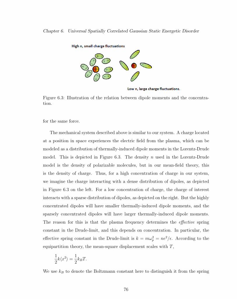
Chapter 6. Universal Spatially Correlated Gaussian Static Energetic Disorder
Figure 6.3: Illustration of the relation between dipole moments and the concentra-tion.
for the same force.
The mechanical system described above is similar to our system. A charge located
at a position in space experiences the electric field from the plasma, which can be
modeled as a distribution of thermally-induced dipole moments in the Lorentz-Drude
model. This is depicted in Figure 6.3. The density n used in the Lorentz-Drude
model is the density of polarizable molecules, but in our mean-field theory, this
is the density of charge. Thus, for a high concentration of charge in our system,
we imagine the charge interacting with a dense distribution of dipoles, as depicted
in Figure 6.3 on the left. For a low concentration of charge, the charge of interest
interacts with a sparse distribution of dipoles, as depicted on the right. But the highly
concentrated dipoles will have smaller thermally-induced dipole moments, and the
sparsely concentrated dipoles will have larger thermally-induced dipole moments.
The reason for this is that the plasma frequency determines the effective spring
constant in the Drude-limit, and this depends on concentration. In particular, the
effective spring constant in the Drude-limit is k = mω2p = ne2/ε. According to the
equipartition theory, the mean-square displacement scales with T ,
1
2k〈x2〉 =
1
2kBT.
We use kB to denote the Boltzmann constant here to distinguish it from the spring
76

Chapter 6. Universal Spatially Correlated Gaussian Static Energetic Disorder
constant k. The average of the square of the dipole moment is therefore
〈p2〉 = e2〈x2〉 =e2kBT
k.
On the other hand, the energy due to charge-dipole interactions is a sum over sur-
rounding dipoles in the Coulomb field of the charge,
u = −∑i
p(ri) · E(ri) = −∑i
ep(ri)
4πε
1
r2i
. (6.7)
We are interested in the fluctuation felt by the charge, so we look at the average of
the square,
〈u2〉 =e2
(4πε)2
∑ij
〈p(ri)p(rj)〉1
r2i r
2j
=e2
(4πε)2
∑i
〈p2(ri)〉1
r4i
=e2
(4πε)2
e2kBT
k
∑i
1
r4i
Here we use the fact 〈p(ri)p(rj)〉 = δij since dipoles at different locations are uncor-
related. The last step is to write the summation as an integral by inserting a uniform
density of dipoles n and by excluding the radius to the nearest dipole r = a. The
result is that the variance σ2 = 〈u2〉 is
σ2 =ne4
(4πε)2
kBT
k
∫ ∞a
dr4πr2 1
r4
=ne4
4πε2kBT
mω2pa
=e2
4πεakT. (6.8)
Note, in going to the last line, we substituted ω2p = ne2
mεm and the n in the numerator
canceled the n in the denominator. This is the exactly the site-energy variance we
found in Eq. (6.5) (without the Clausius-Mossotti enhancement).
77

Chapter 6. Universal Spatially Correlated Gaussian Static Energetic Disorder
6.4 Universal Reorganization Energy and Univer-
sal Hopping Rate
The plasmon reorganization energy is given by
λpl =∑qω
|gqω|2|eiq·r1−eiq·r2 |2~ω
=3
8
3e2
8πεa, with Clausius-Mossotti enhancement
e2
4πεa, without Clausius-Mossotti enhancement.
(6.9)
For excluded radius a = 1 nm and dielectric permittivity ε = 3ε0, this has a magni-
tude
λpl ∼
0.25 eV , with Clausius-Mossotti enhancement
0.18 eV , without Clausius-Mossotti enhancement
(6.10)
The plasmon reorganization energy is also independent of charge concentration n.
Thus, the hopping rate is universal
R =V 2
~
√π
λphkTe−(δε+ε2−ε1+λph+λpl)
2/4λphkT (6.11)
It depends on ε and λpl arising from interactions between charges, but is independent
of their concentration.
6.5 One-Dimensional Mobility
Since our site-energy correlation function has the same algebraic decay as in the
charge-dipole model 〈u(0)u(r)〉 ∼ 1/r, it is straightforward to substitute this hopping
rate into expressions of the field-dependent mobility addressed in Chapter 3. The
simplest application is to use the rate in the analytic expression for mobility in one-
dimension. The a in our model becomes the lattice constant ρ in reference [37, 46].
78

Chapter 6. Universal Spatially Correlated Gaussian Static Energetic Disorder
In terms of lattice sites, our correlation function becomes
〈u(r1)u(rn+1)〉 ≡ 〈u1un+1〉 = σ2
1/n , if n ≥ 2
3/4 , if n = 1. (6.12)
Using the correlation in [37], we find an analytical expression of the Poole-Frenkel
mobility for our plasmon-phonon problem,
µ = µ0e−β∆
2 e−1516β2σ2
e2βσ√βeEρ, (6.13)
where
∆ =λph + λpl
2,
and
µ0 =eρ2
kT
V 2
~√
∆kT
√1− σ2
8∆kT
(βeEρ)1/4 (βσ)1/2.
This is remarkably similar to the result using the charge-dipole mechanism for
correlated disorder. One caveat is that our σ here is temperature dependent, increas-
ing as√T . So Arrhenius plots will show a weaker linear dependence on T−1, in line
with Gill’s parametrization rather than Bassler’s parametrization [43].
6.6 Concluding Remarks
We have shown that spatially (nearly static) correlated Gaussian energetic disorder
arising from charge-charge interactions has standard deviation σ ∼ 0.11 eV and site
energy correlation 〈u(0)u(r)〉 ∼ 1/r. This shows a good agreement with both the
energy scale and the correlation form for the correlated-disorder produced by the
charge-dipole interaction. One remarkable outcome is that, although the disorder
is caused by charge-charge interactions, the disorder does not depend on charge
79

Chapter 6. Universal Spatially Correlated Gaussian Static Energetic Disorder
concentration. This is universal static disorder. The field-dependent mobility is the
same as in the charge-dipole model, which shows that the Poole-Frenkel law does
not necessarily require a minimum concentration of dipoles for its validity.
80

Chapter 7
Is Disorder Due to Plasma
Fluctuations Static?
7.1 Introduction
In the previous chapter we showed how the full width of the energetic disorder
depends on integrating over the Lorentzian of distribution of frequencies (see Eq.
(6.6)). A Lorentzian has a long (algebraic) tail, and obviously the highest frequency
contributions out in the tail cannot be considered as part of the static disorder. To
represent this in the simplest possible manner, let us divide the frequency interval
into two regions, above and below a cut-off frequency ωc. Plasma oscillating with
ω ≤ ωc will be considered as contributing to static disorder, and plasma oscillating
with ω > ωc will be considered as contributing to dynamic disorder.
It follows that the Lorentzian integral over frequency in Eq. (6.6) should be cut
off, so that∫ ωc
0
2
π
Γ−ω2 + Γ2
−dω =
2
πtan−1
(ωcΓ−
), (7.1)
81

Chapter 7. Is Disorder Due to Plasma Fluctuations Static?
implying that the variance of the static disorder is given by
σ2 = σ20
2
πtan−1
(ωcΓ−
), (7.2)
where σ20 = 3e2
8πεakT is the full variance calculated in Eq. (6.6). (Without Clausius-
Mossotti enhancement, the full variance is σ20 = e2
4πεakT .)
In this chapter, we will examine the relevant time scales that determine ωc. We
argue that ωc depends on the mobility, and since the mobility depends on the level
of static disorder, and as this is dependent on ωc, we are led to a self-consistent
equation for the amount disorder in the system that can be considered to be static,
and the amount that should instead be considered to be dynamic. This will be used
to determine the dependence of the mobility on the concentration of charge.
7.2 Determination of the Static/Dynamic Cutoff
Frequency ωc
A number of different time scales are evident in our system. Let us list them first,
before discussing which should be used to determine ωc.
• R: the hopping rate between two isoenergetic sites.
• Resc: the escape rate for a charge leaving a trap.
•√λphkT/~: the decaying rate of the phonon memory function, in (the Gaussian
approximation).
• Γ: The characteristic frequency for a dielectric in the Debye limit; the width
of the Lorentzian distribution.
82

Chapter 7. Is Disorder Due to Plasma Fluctuations Static?
Since σ2 will be determined by ωc/Γ, let us first review what it is that determines Γ.
As we have discussed previously, in the Drude model,
Γ =ne2
mεγ=ne
εµ. (7.3)
The Lorentzian width Γ is determined by the charge concentration and the mobility
µ = (mγ)−1. It is important to keep in mind that the frequency at which plasma
fluctuations heal, i.e., restore neutrality, is not just set by their susceptibility to
move in an applied field, but also by their concentration. The mobility can be very
high, and the rate of decay of charge density fluctuations can still be low if the
concentration is sufficiently low. For n ∼ (1/100 nm)3 and µ ∼ 10−3 cm2/V s and
ε = 3ε0), Γ ∼ 104 s−1. From simulations by Bassler et al. [33] it has been known
that typical hopping rates in the absence of disorder should be about R ∼ 1012 s−1.
Thus there is no question that many thousands of hops can take place before plasma
reorganization. In this case, R/Γ = 108!
The memory function decay rate has to be faster than the rate, so the validity of
the linearization (in τ) of the plasmon memory function is not in question.
Thus all we need to concern ourselves with is the trap escape rate Resc. For
sufficiently high disorder, the transport in these systems is trap limited. The charges
spread most of their time in low-energy states, or in the case of spatially correlated
disorder, in clusters of low energy sites (see Figure 3.9.). In fact, the Poole-Frenkel
field dependence comes about as lowering of the energetic barrier for release from
a broad cluster of trap sites [74]. By trap limited, we mean that the time a charge
spends outside of a trap is negligible compared to the time spent residing in a trap.
The criteria for considering whether the plasma fluctuations may or may not be
considered as static disorder insofar as transport is concerned hinges, therefore, on
whether a low-energy cluster of sites will remain stationary longer than the time for
a charge to escape such a cluster. Thus the cut-off frequency below which oscilla-
83

Chapter 7. Is Disorder Due to Plasma Fluctuations Static?
tions may be considered to be static is ωc ∼= Resc , where Resc is the characteristic
trap escape-rate. Trap-limited transport is often described in terms of the Multiple
Trapping Model, a model of economy in which the energetic manifold is segregated
into a transport level along which charges readily diffuse, punctuated by isolated
low-energy traps at some trap energy εT . In equilibrium, the escape rate Resc from
the trap manifold and the trapping rate Rtrap from the free-state manifold are related
one another through detail balance,
Resc =PfreePtrap
Rtrap. (7.4)
Here Pfree is the probability that a charge is free, and Ptrap is the probability that a
charge is trapped. These can be written in terms of the partition functions Ztrap =
VtrapeβεT and Zfree = Vfree, where Vtrap and Vfree are the respective manifold volumes.
We have
Ptrap =Ztrap
Ztrap + Zfree∼= 1,
and
Pf =Zfree
Ztrap + Zfree∼=VfreeVtrap
e−βεT =e−βεT
c,
where c = Vtrap/Vfree is the trap (volume) ratio. In the trap-limited regime, although
c is small, eβεT is large so that the product ceβεT 1. It follows that Pfree/Ptrap ∼=
e−βεT /c, and therefore that
Resc∼= Rtrap
e−βεT
c.
On the other hand, for a dilute set of traps we will use the Smoluchowski diffusion-
limited trapping rate, [121], writing
Rtrap = 4πDrtrapntrap, (7.5)
in terms of which the escape rate becomes
Resc = 4πDrtrape−βεT .
ntrapc
84

Chapter 7. Is Disorder Due to Plasma Fluctuations Static?
Here D is the diffusion constant for the free state manifold, rtrap is the trap radius,
and ntrap is the trap concentration. At the same time, the trap-limited mobility
µ =eD
kTPfree =
eD
kT
e−βεT
c
is the mobility in the free state manifold eD/kT multiplied by Pfree. It follows that
the ratio in Eq. (7.2) determining the level of static disorder,
ωcΓ∼=Resc
Γ=
4πDrtrapntrape−βεTc(
neε
) (e−βεTc
)eDkT
=ntrapn
rtrapr,
is determined by the ratio of the trap concentration to the charge concentration
multiplied by the ratio of the trap radius to the Coulomb radius
r =e2
4πεkT∼ 20 nm. (7.6)
The diffusion constant D in the free-state manifold cancels out. It follows that the
variance of the static disorder
σ2 =2
πσ2
0 tan−1(ntrap
n
rtrapr
). (7.7)
decreases with increasing charge concentration. For spatially correlated disorder we
anticipate rtrap/r ∼ 1 at room temperature The crucial parameter that must be
determined now is the concentration of traps ntrap.
7.3 Trap Concentration for Gaussian Energy Den-
sity of States
The crucial part of Eq. (7.7) that remains to be determined is the trap concentration
ntrap. For hopping in a Gaussian manifold, there are many low energy sites that
establish traps; the trap/free dichotomy of the Multiple Trapping Model does not
85

Chapter 7. Is Disorder Due to Plasma Fluctuations Static?
simply present itself. On the other hand, we know in the case of spatially-correlated
disorder from the charge-dipole interaction that transport is limited by traps of a
certain critical size and depth [74], and it seems plausible that there should be a way
to estimate this concentration. Actually, there has been much discussion concerning
this very point in the literature concerning uncorrelated Gaussian energetic disorder,
and so we begin with that.
7.3.1 Uncorrelated Gaussian Disorder and Multiple Trap-
ping Model
The procedure by which transport in a Gaussian density of states can be mapped
into the Multiple Trapping Model has been pursued by many investigators, most
notably work by Arkhipov [122, 123]. One imagines dividing the partition function
into two parts by introducing a transport energy ut so that
Z =
∫ ∞−∞
g(u)e−βudu =
∫ ut
−∞g(u)e−βudu+
∫ ∞ut
g(u)e−βudu ≡ Ztrap + Zfree.
(7.8)
Here the density of states is Gaussian,
g(u) =e−u
2/2σ2
√2πσ2
.
The energy associated with the trapping level can be found by completing the square
in the exponent in Ztrap,
Ztrap =
∫ ut
−∞due−u
2/2σ2
√2πσ2
e−βu
=eβ
2σ2/2
√2πσ2
∫ ut
−∞due−β(u+βσ2)
2/2σ2
. (7.9)
86
Chapter 7. Is Disorder Due to Plasma Fluctuations Static?
We see that the integral is peaked at up = −βσ2. We define this peak to be the
trapping energy level, and formally rewrite the partition function
Ztrap ∼= e−βup∫ up+δ
up−δdue−u
2/2σ2
√2πσ2
, (7.10)
where we have pulled out the Boltzmann factor evaluated at u = up, and introduced
a window of integration around u = up that defines the fraction of states to be
associated with this energy. This integral defines the relative concentration of trap
sites,
c ≡∫ up+δ
up−δdue−u
2/2σ2
√2πσ2
. (7.11)
Assuming that ut up, it follows from Eq. (7.9) that
Ztrap ∼= eβ2σ2/2. (7.12)
Comparison of Eq. (7.12) with Eq. (7.10) shows that
c = e−β2σ2/2 (7.13)
Not surprisingly, the effective trap concentration is small, coming from states in the
Gaussian tail, and thus it depends strongly on temperature. This is the quantity
we need to complete our calculation of the static disorder threshold in the previous
section. Before returning to that discussion, however, it is worth mentioning that
one can go further with this to recover the transport energy ut by comparing the
Multiple Trapping Model to results from numerical simulations. For example, from
the three-dimension simulation of Bassler [33], we know that the low-field mobility
is found to be
µ = µ0e−Aβ2σ2
,
where the empirically determined parameter A ∼= 4/9. Comparison with the multiple
trapping model implies that
Pfree =Zfree
Zfree + Ztrap∼=ZfreeZtrap
= e−Aβ2σ2
.
87

Chapter 7. Is Disorder Due to Plasma Fluctuations Static?
The integral Zfree is over the tail part of a displaced Gaussian, and can be approxi-
mated by an asymptotic expression for the error function, with the result that
Zfree ≈1√
2πσ2
σ2
βσ2 − uteβ
2σ2/2e−(βσ2+ut)2/2σ2
. (7.14)
The value of Ztrap is given by Eq. (7.12). Taking the ratio in Eq. (7.14) and
comparing only the exponential behavior, we find
Aβ2σ2 ≈ (βσ2 + ut)2
2σ2.
Solving the quadratic equation for ut, we find the transport energy,
ut = −βσ2(
1−√
2A)≈ −0.06 βσ2 < 0, (7.15)
is slightly below the center of the density of states. Finally, this implies that in the
mapping to the multiple trapping model, the depth below the transport level is
εT = 0.94βσ2. (7.16)
Let us return now to our discussion of the static disorder threshold and the ratio
ntrap/n required in the argument of tan−1 in Eq. (7.7). The trap concentration
ntrap = nsitec = nsitee−β2σ2/2 (7.17)
is given by the concentration of hopping sites multiplied by c from Eq. (7.13).
Expressing the charge density as a fraction x of the number of sites occupied by a
charge, we find
tan
(π
2
σ2
σ20
)=rtrapr
e−β2σ2/2
x(7.18)
For uncorrelated Gaussian disorder, the trap radius is in the size of the hopping
distance a ∼= 1 nm. and so rtrap/r = T/T0, where kT0 = e2/4πεa ∼ 0.5 eV. Eq.
(7.18) has been solved numerically for σ as a function of temperature for x = 10−3,
88

Chapter 7. Is Disorder Due to Plasma Fluctuations Static?
0 0.5 1 1.5
T/300K
0
0.5
1σ2/σ
2 0
10nm
100nm
1000nm
(a) Fraction of plasmonic Gaussian disordervariance that can be considered as static,plotted versus T , parametric in average sep-aration of injected charges.
0 0.5 1 1.5
T/300K
0
5
10
ωc/Γ
−
10nm
100nm
1000nm
(b) Ratio of the cutoff frequency to the di-electric response frequency for different con-centrations of charges.
Figure 7.1: Fraction of disorder that may be considered to be static.
10−6, and 10−9, corresponding to a charge concentration of one charge per 10 nm,
100 nm, and 1000 nm, respectively, as shown in Figure 7.1a. We can see that for
room temperature (T = 300 K), the level of static disorder saturates for the lower
concentrations, indicating universal Gaussian disorder. The lower the concentration,
the more universal.
For high concentration, we observe that σ2/σ20 increases linearly with T , the
leading behavior of an iterated log function. This is interesting since σ20 = 3e2
8πεakT is
already proportional to temperature, implying µ = µ0e−Aβ2σ2
= Cµ0, where C is a
constant, independent of T as far as the plasma disorder is concerned. We can also
obtain the ratio ωc/Γ, shown in Figure 7.1b.
7.3.2 Correlated Disorder Case
At low electric fields, the occupation of sites in a spatially-correlated Gaussian man-
ifold is no different than for the uncorrelated case. Probabilities are still determined
89

Chapter 7. Is Disorder Due to Plasma Fluctuations Static?
by the Boltzmann factor, and the arguments made in the previous subsection re-
garding the effective trap energy up = −βσ2 and the effective trap concentration
c = e−β2σ2/2 remain the same. The empirically-determined mobility µ = µ0e
−Aβ2σ2
from Monte Carlo simulations in Gaussian correlated disorder [50] yield A = 0.36,
a bit smaller than Bassler’s A = 0.44, but this can be understood as arising from a
greater selection of pathways for a charge to escape a trap when the trap is a broad
energetic valley. Indeed, Parris [75] has shown that the value of the parameter A
decreases substantially when the wavefunction decay length is increased, allowing a
charge to escape a low energy site through next-nearest neighbors as well as nearest-
neighbors. Such variable range hopping essentially lowers the effective energy of the
of the transport manifold, since the final state energy in an uphill hop may be chosen
from a compressed distribution function [124]. A more difficult exercise is to assess
how the effective trap concentration should be modified when hopping takes place
at high electric fields, where the mobility shows a Poole-Frenkel field dependence.
Physical understanding of the role of E in tilting broad energetic valleys, so that they
no longer act as traps, suggests that the Poole-Frenkel factor should be attributed
to a lowering of the effective transport energy, leaving the trap level alone. Yet it is
also clear that the broadest (and deepest) valleys no longer act as traps for strong
E; only valleys smaller than a field-dependent radius rc = σ√
βaeE
are rate-limiting.
These valleys tend to be shallower, comprised of sites higher in the Gaussian man-
ifold. Thus we anticipate that the trap level will actually increase along with the
concentration of traps. This makes sense from a physical standpoint. In the electric
field, a charge will spend less time in a trap, so there is less time for rearrangement
of the plasma while the charge is trapped. This means that higher frequency plasma
modes may still be regarded as stationary, as far as trapping of charges is concerned.
In general, we expect that higher fields will increase the static contribution to σ,
in the direction of the saturated value σ0.
90

Chapter 7. Is Disorder Due to Plasma Fluctuations Static?
7.4 Conclusion
The universal Gaussian disorder introduced in Chapter 6 has been examined in
this chapter by introducing a cutoff frequency to exclude the high frequency part
of plasmonic oscillators. This cutoff frequency was determined by the escape rate
for a charge leaving a trap. A transcendental equation for static disorder shows
that universality appears for a sufficiently dilute concentration of charges, or for
sufficiently high temperatures. For room temperature, we find universality for charge
separations on the order of 100 nm or greater; this is the concentration for which
charge-charge interactions will bring about a universal Poole-Frenkel mobility field
dependence.
91

Chapter 8
Epilogue
In this dissertation, we have discussed how the mobility of injected charge in or-
ganic semiconductors is influenced by the mutual interactions between charges. In a
mean-field approximation, we obtained a Hamiltonian formulation of dielectric fric-
tion of which the Frohlich Hamiltonian is a special case. We found a general recipe
with which to generalize the Frohlich Hamiltonian for use with arbitrary forms of
the dielectric susceptibility. Our Hamiltonian replaces charge-charge interactions
with plasmonic oscillators, and provides a picture of a fluctuating energy landscape
disturbing charge transport. Due to the extreme diluteness of injected charge carri-
ers, the characteristic time scale of plasma oscillations is much longer than the time
spent for each hop, so that implementation of the ensemble average over oscillator
states to determine the hopping rate between sites is inappropriate. We revisited
the concept of the ensemble averaged hopping rate and discussed how to consider
the hopping rate in the absence of the ensemble average: plasmonic oscillators are
to be regarded as a source of static disorder. It turns out that the plasmonic static
disorder is spatially correlated Gaussian energetic disorder. It also turns out that
the energy-energy correlation falls off algebraically with distance as r−1, just as in
the case of the charge-dipole model used to explain the Poole-Frenkel field depen-
92

Chapter 8. Epilogue
dence. Moreover, a universality arises, so that the standard deviation is a constant,
independent of charge concentration. To have universality requires that the time for
a charge escaping from a trap is smaller than the relaxation time of the dielectric.
A self-consistent equation determining the amount of static plasmonic disorder was
obtained by appealing to the simplicity of the Multiple Trapping Model. We were
able to show below what concentration and above what temperature plasmonic dis-
order may be considered to be static correlated disorder leading to the Poole-Frenkel
mobility field dependence. These conditions are often satisfied in time-of-flight exper-
iments in which the concentration of carriers is purposefully dilute, to avoid space
charge effects. For these systems, charge-charge interactions may be the primary
cause of the ubiquitous Poole-Frenkel law.
The results presented here are approximate, having been determined from a mean-
field theory. As with all many-body calculations of this nature, even if they lack ac-
curacy, the importance of these methods is that they often elucidate general trends
and scaling behaviors. We are particularly interested in the robustness of the uni-
versal static disorder, and its appearance as a function of charge concentration and
temperature. Are there experimental indicators of universality (other than the ob-
servation of Poole-Frenkel law in systems without sufficient dipoles)? At this time, it
is difficult to say. Data has not been examined with this model in mind, and it will
take careful examination to assess the importance of the new ideas presented here.
An obvious drawback is that the concentrations where we have predicted univer-
sality concern charge separations that are approximately the size (100 nm) of many
modern thin film devices. The universal aspects of the long-range Coulomb interac-
tion rely on integrating out to infinity, as though we were dealing with bulk materials.
Thus, the level of charge-charge static disorder may be strongly dependent on device
geometry, and should be considered if our ideas are going to be useful for the design
of organic electronics. This, we anticipate, will be one of the primary directions of
93

Chapter 8. Epilogue
future work based on the model presented here.
94

Appendices
A Justification of Fermi Golden Rule
B Frohlich Hamiltonian
C Displaced Oscillator Transformation
D The Physical Meaning of sin2(qa)/q2a2
95

Appendix A
Justification of Fermi’s Golden
Rule
Although the Schrodinger equation is often solved in the time domain to observe
the time evolution of the quantum state directly, the Green function technique for-
mulating the evolution in the reciprocal time domain has distinct advantages. In
this Appendix, we will demonstrate how to solve the time-dependent Schrodinger
equation via the Green function technique. After carrying out the displacement
transformation, we have
H = H0 +Hhop
H0 = (ε1 − g2~ω)|Φ1〉〈Φ1|+ (ε2 − g2~ω)|Φ2〉〈Φ2|+ ~ω(b†b+1
2)
Hhop = V O†|Φ1〉〈Φ2|+ V O|Φ2〉〈Φ1|
O = eg(b−b†)(eik·r1−eik·r2 )
The diagonal Hamiltonian H0 has eigenfunctions |Φ1(2)〉|n〉 with eigenenergies ε1(2)n=
ε1(2) + n~ω. The off-diagonal Hamiltonian Hhop drives the transition between the
|Φ1〉 and |Φ2〉 manifolds. Assume the initial condition |Ψ(0)〉 = |Φ1ni〉 describes
96

Appendix A. Justification of Fermi’s Golden Rule
the particle located at site 1 with a certain phonon state |ni〉. We would like to
answer the question, what is the rate at which a particle leaves site 1? The Green
function method is implemented in the Fourier domain. We take the one sided
Fourier transform of the Schrodinger equation first to get
i~(−|Ψ(0)〉 − iz
~|Ψ(z)〉
)= H|Ψ(z)〉 (A.1)
or,
|Ψ(z)〉 =i|Ψ(0)〉z −H/~
. (A.2)
Here the general wave function is of the form |Ψ(z)〉 = c1i(z)|Φ1ni〉+∑
f c2f (z)|Φ2nf〉
and z is the Fourier variable. The second term includes the possible final phonon
states denoted by nf . The inverse transformation gives
|Ψ(t)〉 =1
2π
∫ ∞−∞
dze−izt/~|Ψ(0)〉
z −H + iη, (A.3)
where η → 0+ is a convergence factor. The poles located in the denominator deter-
mine the temporal characteristic of the solution. That is, if poles are located along
the real axis, the initial state shows an oscillatory behavior. By contrast, if poles
have negative imaginary parts, the initial state will decay exponentially in time. The
Green function is defined as
G(z) =1
z −H + iη=
1
z −H0 −Hhop + iη
Introducing the unperturbed Green function,
G0(z) =1
z −H0 + iη,
it is easily shown that,
G(z) = G0(z) +G0HhopG(z) = G0(z) +G(z)HhopG0(z), (A.4)
97

Appendix A. Justification of Fermi’s Golden Rule
which is known as the Dyson equation. Since |Φnnk〉 is an eigenstate of G0, we can
compute the diagonal matrix element of the Green function
G1i1i(z) ≡ 〈Φ1ni|G(z)|Φ1ni〉
= G01i1i +G01i1i
∑i′,f
H1i2fG02f2fH2f1i′G1i′1i
=1
z − ε1i −∆(z) + iη, (A.5)
where H1i2f ≡ 〈Φ1ni|Hhop|Φ2nf〉 and G01i1i ≡ 〈Φ1ni|G0|Φ1ni〉. The quantity ∆(z) is
called the self-energy,
∆(z) =∑f
|H1i2f |2
z − ε2f + iη=∑f
〈1i|Hhop|2f〉〈2f |Hhop|1i〉z−ε2f+iη
(A.6)
This has been obtained in an approximation. In Eq. (A.5), we have restricted the
sum over phonon state i′ visited with the return of the particle to site 1 to include
only the initial phonon state i. With this restriction, the expression of G is closed,
i.e. G is determined to all orders. This approximation is known as the method of
Wigner and Weisskopf. The coefficient c1i(t) is obtained by projecting eq.(A.3) on
〈Φ1ni|, namely,
c1i(t) = 〈Φ1ni|Ψ(t)〉 = − 1
2π
∫ ∞−∞
dze−izt/~G1i1i(z)
The poles of the Green function determine the time behavior of the state. For
instance, the simplest case is that ∆(z) = 0 meaning the two manifolds |Φ1ni〉 and
|Φ2nf〉 are decoupled. In this case the Green function G1i1i(z) has a simple pole ε1i−iη
at the lower complex plane. It follows that c1i = e−iε1it/~ is simply a phase factor since
the charge stays at the initial state of the system. Going beyond this simple case, we
seek the solutions of z − ε1i −∆(z) + iη = 0 to find poles. The iteration method of
solution is generally applied, with the algorithm as follows. First, the zeroth solution
is found by assuming ∆(z) = 0 with the at z0 = ε1i − iη. Next, we replace ∆(z) by
∆(z0) to obtain the first order solution z1 = ε1i+∆(z0)−iη. Continuing the iteration
98
Appendix A. Justification of Fermi’s Golden Rule
until we reach zn+1 ≈ zn or ∆(zn) ≈ ∆(zn−1), the self-consistent solution for z is then
found. Let us take the previous example showing the zeroth order solution further
to obtain the first order solution. We then have
∆(z0)= limη→0+
∑f
〈Φ1ni|H|Φ2nf〉〈Φ2nf |H|Φ1ni〉ε1i−ε2f+iη
=−i~
∫ ∞0
dt∑f
ei(ε1i−ε2f )t/~〈Φ1ni|H|Φ2nf〉〈Φ2nf |H|Φ1ni〉
c1i(t)=− 1
2πilimη→0+
∫ ∞−∞dze−izt/~
1
z − ε1i −∆(z0) + iη
= e−i(ε1i+∆(z0))t/~
The probability to remain in the initial state is
P1i(t) = |c1i(t)|2 = e−i(∆−∆∗)t/~ ≡ e−Rt
With a little algebra, one can show that
∆(z0) = −iV2
~
∫ 0
−∞dtei(ε2−ε1)t/~〈ni|O(0)O(t)|ni, 〉
∆∗(z0) =iV 2
~
∫ ∞0
dtei(ε2−ε1)t/~〈ni|O(0)O(t)|ni〉,
and
i(∆−∆∗)
~=V 2
~2
∫ ∞−∞dtei(ε2−ε1)t/~〈ni|O(0)O(t)|ni〉,
which is the decay rate above. This is a remarkable expression for it shows that the
imaginary part of the self-energy is the Fermi golden rule rate,
R ≡ −i(∆−∆∗)
~=
2=∆(z0)~
=V 2
~2
∫ ∞−∞dtei(ε2−ε1)t/~〈ni|O(0)O(t)|ni〉 (A.7)
The first order iterative solution z1 gives us the equivalent result of the Fermi Golden
rule. It implies that if the first order solution is satisfactory, the self-energy should
remain nearly the same as we go through further iterations. Since ∆(z2) u ∆(z1),
99

Appendix A. Justification of Fermi’s Golden Rule
we end up with the relation,
∆(z2)=−i~
∫ ∞0
dt∑f
ei(ε1i−ε2f+∆(z1))t/~〈Φ1ni|H|Φ2nf〉〈Φ2nf |H|Φ1ni〉
and therefore
i(∆(z2)−∆∗(z2))
~=V 2
~2
∫ ∞−∞dtei(ε2−ε1+∆(z1))t/~〈ni|O(0)O(t)|ni〉
uV 2
~2
∫ ∞−∞dtei(ε2−ε1)t/~〈ni|O(0)O(t)|ni〉
To satisfy this condition, we require that during the decay of the memory function,
the additional phase factor ei∆(z1)t/~ ∼ 1. If we define the time scale for the memory
function decay to be τ , this implies that
∆
~τ 1; or
~∆ τ
Since the imaginary part of the self-energy is the Fermi golden rule rate, we arrive
at the self-consistent criteria for the validity of the Fermi golden rule,
1
R τ ;
The memory function must decay in a time τ shorter than the time for a hop.
100

Appendix B
Frohlich Hamiltonian
Frohlich [21,22] proposed an empirical interaction mechanism to describe an electron
passing through a dielectric or a polar crystal. He treated the dielectric or the polar
crystal as an isotropic continuum in a mean field approximation. The Lorentz model
is chosen to describe the response subject to an external electric field. For a given
displacement X of an oscillator in an unit cell with reduced mass m and natural
frequency ω0, the force formula reads
md2X
dt2+mω2
0X = e∗E,
where e∗ is an effective charge participating the distortion and E is an external
electrical field. It follows that an induced dipole moment P couples to a moving
electron at position r0 via the Coulomb interaction according to
Hint =
∫drP(r) · ∇V (r) = −
∫dr∇ ·P(r) V (r)
P(r) =N
L3e∗ X(r)
V (r) = − e
4πε0
1
|r− r0|,
where N denotes the number of unit cells within the total volume L3. This dis-
placement can be written in terms of a superposition of Fourier components in q
101
Appendix B. Frohlich Hamiltonian
space
X(r) =1√N
∑q
Xqeiq·r =
∑q
√~
2NmωL
(eqbqe
iq·r + e∗qb†qe−iq·r) ,
where eq is a polarization unit vector and ωL is the longitudinal optical frequency
since only the longitude mode contributes to interactions. Here we have written Xq
in terms of second quantized notation with the creation and annihilation operator
b†q and bq respectively. The polarization charge density is
−∇ ·P(r) = −NVe∗∑q
√~
2NmωL
(eq · iqbqeiq·r − e∗q · iqb†qe−iq·r
), (B.1)
and the interaction Hamiltonian becomes
Hint =Ne∗e
L34πε0
√~
2NmωL
∑q
eq · iq∫dr
1
|r− r0|(bqe
iq·r − b†qe−iq·r)
= iNe∗e
L3ε0
√~
2NmωL
∑q
1
q
(bqe
iq·r0 − b†qe−iq·r0).
Combined with the associated Lyddane-Sachs-Teller relation [108–110, 125], ε(0)ε(∞)
=ω2L
ω20, we can find the effective charge
e∗ = ε0ωL
√mL3
N
√1
ε(∞)− 1
ε(0)
With this, the interaction Hamiltonian becomes
Hint = i~ωL
√e2
2L3~ωL
∑q
1
q
(bqe
iq·r0 − b†qe−iq·r0)
≡∑q
igq~ωL(bqe
iq·r0 − b†qe−iq·r0)
gq ≡
√e2
2L3~ωL1
q
We can then introduce the dimensionless scalar momentum operator Pq =(bq−b†−q)√
2i
to cast the interaction Hamiltonian in the form
Hint = −√
2∑q
gq~ωLPqeiq·r0
102

Appendix B. Frohlich Hamiltonian
In summary, the Frohlich Hamiltonian is understood as an empirical model to de-
scribe the linear electron-phonon coupling for which the momentum coordinate cou-
ples to the charge motion. Our derivation (in the text) of the same Hamiltonian
from the perspective of dielectric friction is based on different physical intuition.
103

Appendix C
Displaced Oscillator
Transformation
The polaron Hamiltonian describes a two-state system coupled with a bosonic bath
comprised of harmonic oscillators with a spectrum of normal modes. For simplicity,
a single band ωk with the wavevector k is considered. The Hamiltonian is written as
H =2∑
n=1
εn|Φn〉〈Φn|+ V (|Φ1〉〈Φ2|+ |Φ2〉〈Φ1|)
+∑k
~ωk
(b†kbk +
1
2
)+∑k
gk(bk + b†−k)(eik·r1|Φ1〉〈Φ1|+ eik·r2 |Φ2〉〈Φ2|)
(C.1)
Here εn denotes the site energy for site n, V the hopping matrix element, and gk a
linear coupling constant at a particular k mode. The basis function |Φn〉 satisfies
the orthogonality condition 〈Φn|Φm〉 = δnm, and b(†)k is the annihilation (creation)
for bosons associated with the frequency ωk. The coupling term shows the strength
of linear coupling to the displacement of oscillators at each mode is determined by
gk. The role of the displaced oscillator (or polaron) transformation is to get rid of
the linear coupling term by translating the undistorted equilibrium points for all
104

Appendix C. Displaced Oscillator Transformation
oscillators to equilibrium points where oscillators are no longer coupled. To perform
aa unitary transformation we generally sandwich the Hamiltonian between U = e−D
and U † = eD,
H = e−DHeD.
For computational convenience, we will write the Hamiltonian in terms of Pauli
matrices
H =ε1 + ε2
2I +
ε1 − ε2
2σz + V σx +
∑k
~ωk
(b†kbk +
1
2
)+∑k
g+k (bk + b†−k)I +
∑k
g−k (bk + b†−k)σz (C.2)
g+k = gk
eik·r1 + eik·r2
2
g−k = gkeik·r1 − eik·r2
2
(C.3)
The displacement operator is of the form,
D =2∑
n=1
∑k
gk(bk − b†−k)eik·rn|Φn〉〈Φn|
=∑k
g+k (bk − b†−k)I +
∑k
g−k (bk − b†−k)σz (C.4)
Here are some useful relations:
e−DσxeD = e−2
∑k g−k (bk−b†−k)|Φ1〉〈Φ2|+ e2
∑k g−k (bk−b†−k)|Φ2〉〈Φ1|
e−Db†keD = b†k − g
+k I− g
−k σz
e−DbkeD = bk − g∗+k I− g∗−k σz
105

Appendix C. Displaced Oscillator Transformation
Taking advantage of these relations, we find the transformed Hamiltonian,
H =2∑
n=1
(εn −
∑k
|gk|2~ωk
)|Φn〉〈Φn|+
∑k
~ωk
(b†kbk +
1
2
)+ V e−
∑k gk(bk−b†−k)(eik·r1−eik·r2 )|Φ1〉〈Φ2|
+ V e∑
k gk(bk−b†−k)(eik·r1−eik·r2 )|Φ2〉〈Φ1| (C.5)
We can see that while the coupling term is completely removed, what is new is a
lowering of the site energy by the polaron binding energy∑
k |gk|2~ωk, and a mod-
ification of the transfer matrix element V e−∑
k gk(bk−b†−k)(eik·r1−eik·r2 ). The displaced
oscillator transformation is obviously useful when V is the small quantity for a per-
turbation expansion.
106

Appendix D
The Physical Meaning of
sin2(qa)/q2a2
In Eq. (6.3) we inserted a factor sin2(qa)/q2a2 to avoid a divergence at q →∞. We
can think of this factor as a modification of the coupling constant gqω, namely,
gqω =
√e2
2εL3~ω1
q→√
e2
2εL3~ω1
q
sin(qa)
qa(D.1)
In this section we are going to describe what this modification means physically.
To find the equation of motion of a moving particle, we start with the Hamiltonian
H =p2
2m+ U(r) +
∑qω
~ω2
(PqωP−qω +XqωX−qω + 23/2gqωXqωe
iq·r) (D.2)
Writing Hamilton’s equations, we find
p = −∇U(r(t))−∑qω
√2~ωgqωXqω(t)iqeiq·r(t)
Xqω(t) = −√
2ω2g−qω
∫ t
−∞dt′
sin(ω(t− t′))ω
e−iq·r(t′)
107

Appendix D. The Physical Meaning of sin2(qa)/q2a2
Writing the equations above in continuous q space leads to
p = −∇U(r(t))−∑ω
√2~ω
L3
(2π)3
∫dq gω(q)Xω(q, t)iqeiq·r(t) (D.3)
Xω(q, t) = −√
2ω2gω(−q)
∫ t
−∞dt′
sin(ω(t− t′))ω
e−iq·r(t′)
We realize Eq. (D.3) exhibits an inverse Fourier transformation representation
p = −∇U(r(t))−∑ω
√2~ωL3F−1gω(q)Xω(q, t)iq(r(t))
= −∇U(r(t))−∑ω
√2~ωL3
∫dr′F−1qXω(q, t)(r′)F−1igω(q)q(r(t)−r′)
Here we have used the convolution theorem in the second line. It is then straight-
forward to compute the inverse.
F−1qXω(q, t)(r′) =−∫ t
−∞dt′
sin(ω(t−t′))ω
√2ω2
(2π)3
∫dqeiq·(r
′−r(t′))qgω(−q)
=−∫ t
−∞dt′√
2ω2 sin(ω(t−t′))ω
√e2
2εL3~ωδ(|r′−r(t′)|−a)
4πa|r′−r(t′)|
F−1igω(q)q(r(t)−r′) = −√
e2
2εL3~ω1
4π
r(t)−r′
|r(t)−r′|3Θ(|r(t)−r′| − a), (D.4)
where Θ(x) is a unit step function. We obtain
p =−∇U(r(t))
−∑ω
∫dt′ω2 sin(ω(t−t′))
ω
∫dr′
δ(|r′−r(t′)|−a)
4πa2
e
4πε
r(t)−r′
|r(t)−r′|3Θ(|r(t)−r′|−a)
=−∇U(r(t))−∫dt′Γe−Γ(t−t′)
∫dr′eδ(|r′−r(t′)|−a)
4πa2
e
4πε
r(t)−r′
|r(t)−r′|3Θ(|r(t)−r′|−a)
≡−∇U(r(t)) + e E(r(t))
This equation gives the net force experienced by a moving charge at r(t). The second
term is the electric field felt by the charge,
E(r(t)) =
∫dr′ρind(r
′, t)1
4πε
r(t)−r′
|r(t)−r′|3Θ(|r(t)−r′|−a), (D.5)
108

Appendix D. The Physical Meaning of sin2(qa)/q2a2
where
ρind(r′, t) =
∫ t
−∞dt′Γe−Γ(t−t′)eδ(|r′−r(t′)|−a)
4πa2(D.6)
is the image charge density induced in the locations visited previously. The electric
field E(r(t)) is a modified form of the Coulomb field via a step function that implies
the mutual interactions vanish if the spatial distance between the free charge and
the induced charges is less than a. This is exactly what we desire of the mean field
theory at short range. With the help of this step function, we exclude a cavity with
radius a. The other effect of sin(qa)/qa comes into play in the spatial distribution
of the induced charges ρind(r′, t). The polarization exhibits a shell-like geometry
with origin r(t′). When we place a point charge at a certain point, the induced
polarization forms in a spherical shell of radius a surrounding that point. A free
charge experiences a back-attraction to a continuous string of shell-like polarizations
with their origins situated at locations the moving charge visited previously.
109
References
[1] M. Pope and C.E. Swenberg. Electronic Processes in Organic Crystals andPolymers. Oxford University Press, 1999.
[2] P.M. Borsenberger and D.S. Weiss. Organic Photoreceptors for Xerography.Taylor & Francis, 1998.
[3] P.W.M. Blom and M.C.J.M. Vissenberg. Charge transport in poly(p-phenylenevinylene) light-emitting diodes. Materials Science and Engineering: R: Re-ports, 27(34):53 – 94, 2000.
[4] A. Dodabalapur, L. Torsi, and H. E. Katz. Organic transistors: Two-dimensional transport and improved electrical characteristics. Science,268(5208):270–271, 1995.
[5] Sebastian Reineke, Frank Lindner, Gregor Schwartz, Nico Seidler, KarstenWalzer, Bjorn Lussem, and Karl Leo. White organic light-emitting diodeswith fluorescent tube efficiency. Nature, 459(7244):234–238, May 2009.
[6] M. Granstrom, K. Petritsch, A. C. Arias, A. Lux, M. R. Andersson, andR. H. Friend. Laminated fabrication of polymeric photovoltaic diodes. Na-ture, 395(6699):257–260, Sep 1998.
[7] R. H. Friend, R. W. Gymer, A. B. Holmes, J. H. Burroughes, R. N. Marks,C. Taliani, D. D. C. Bradley, D. A. Dos Santos, J. L. Bredas, M. Logdlund,and W. R. Salaneck. Electroluminescence in conjugated polymers. Nature,397(6715):121–128, Jan 1999.
[8] Stephen R. Forrest. The path to ubiquitous and low-cost organic electronicappliances on plastic. Nature, 428(6986):911–918, Apr 2004.
[9] Christopher R. Newman, C. Daniel Frisbie, Demetrio A. da Silva Filho, Jean-Luc Bredas, Paul C. Ewbank, and Kent R. Mann. Introduction to organic thin
110

References
film transistors and design of n-channel organic semiconductors. Chemistry ofMaterials, 16(23):4436–4451, 2004.
[10] Veaceslav Coropceanu, Jerome Cornil, Demetrio A. da Silva Filho, YoannOlivier, Robert Silbey, and Jean-Luc Bredas. Charge transport in organicsemiconductors. Chemical Reviews, 107(4):926–952, 2007.
[11] Jana Zaumseil and Henning Sirringhaus. Electron and ambipolar transport inorganic field-effect transistors. Chemical Reviews, 107(4):1296–1323, 2007.
[12] Oksana Ostroverkhova. Organic optoelectronic materials: Mechanisms andapplications. Chemical Reviews, 116(22):13279–13412, 2016. PMID: 27723323.
[13] Jean-Luc Bredas, David Beljonne, Veaceslav Coropceanu, and Jerome Cornil.Charge-transfer and energy-transfer processes in -conjugated oligomers andpolymers: a molecular picture. Chemical Reviews, 104(11):4971–5004, 2004.PMID: 15535639.
[14] Henning Sirringhaus, Nir Tessler, and Richard H. Friend. Integrated optoelec-tronic devices based on conjugated polymers. Science, 280(5370):1741–1744,1998.
[15] Michele Muccini. A bright future for organic field-effect transistors. Nat Mater,5(8):605–613, Aug 2006.
[16] F. Cicoira and C. Santato. Organic Electronics: Emerging Concepts and Tech-nologies. Wiley, 2013.
[17] G. Nisato, D. Lupo, and S. Ganz. Organic and Printed Electronics: Funda-mentals and Applications. Pan Stanford Publishing, 2016.
[18] A. Buckley. Organic Light-emitting Diodes (OLEDs): Materials, Devices andApplications. Woodhead Publishing series in electronic and optical materials.Elsevier Science & Technology, 2013.
[19] G. Meller and T. Grasser. Organic Electronics. Advances in Polymer Science.Springer Berlin Heidelberg, 2009.
[20] A.R. Brown, C.P. Jarrett, D.M. de Leeuw, and M. Matters. Field-effect transis-tors made from solution-processed organic semiconductors. Synthetic Metals,88(1):37 – 55, 1997.
[21] H. Frohlich. Electrons in lattice fields. Advances in Physics, 3(11):325–361,1954.
111

References
[22] H. Frohlich, H. Pelzer, and S. Zienau. Xx. properties of slow electrons in polarmaterials. The London, Edinburgh, and Dublin Philosophical Magazine andJournal of Science, 41(314):221–242, 1950.
[23] P.W. Atkins and R.S. Friedman. Molecular Quantum Mechanics. OUP Oxford,2011.
[24] Marco Pagliai, Carlo Cavazzoni, Gianni Cardini, Giovanni Erbacci, MicheleParrinello, and Vincenzo Schettino. Anharmonic infrared and raman spectrain carparrinello molecular dynamics simulations. The Journal of ChemicalPhysics, 128(22):224514, 2008.
[25] Y. C. Cheng, R. J. Silbey, D. A. da Silva Filho, J. P. Calbert, J. Cornil, and J. L.Bredas. Three-dimensional band structure and bandlike mobility in oligoacenesingle crystals: A theoretical investigation. The Journal of Chemical Physics,118(8):3764–3774, 2003.
[26] R.E. Peierls. More Surprises in Theoretical Physics. Princeton series in physics.Princeton University Press, 1991.
[27] A. J. Heeger, S. Kivelson, J. R. Schrieffer, and W. P. Su. Solitons in conductingpolymers. Rev. Mod. Phys., 60:781–850, Jul 1988.
[28] W. P. Su, J. R. Schrieffer, and A. J. Heeger. Solitons in polyacetylene. Phys.Rev. Lett., 42:1698–1701, Jun 1979.
[29] E. Kaxiras. Atomic and Electronic Structure of Solids. Cambridge UniversityPress, 2003.
[30] John D. Andersen, C. B. Duke, and V. M. Kenkre. Injected electrons in naph-thalene: Band motion at low temperatures. Phys. Rev. Lett., 51:2202–2205,Dec 1983.
[31] L. B. Schein and A. Tyutnev. The contribution of energetic disorder to chargetransport in molecularly doped polymers. J. Phys. Chem. C, 112:7295, 2008.
[32] Andrey Tyutnev, Vladimir Saenko, and Evgenii Pozhidaev. Dipolar disorderformalism revisited. Chemical Physics, 389(13):75 – 80, 2011.
[33] H. Bassler. Charge transport in disordered organic photoconductors a montecarlo simulation study. physica status solidi (b), 175(1):15–56, 1993.
[34] D. H. Dunlap, P. E. Parris, and V. M. Kenkre. Charge-dipole model for theuniversal field dependence of mobilities in molecularly doped polymers. Phys.Rev. Lett., 77:542–545, 1996.
112

References
[35] H. Bassler, P. M. Borsenberger, and R. J. Perry. Charge transport inpoly(methylphenylsilane): The case for superimposed disorder and polaron ef-fects. Journal of Polymer Science Part B: Polymer Physics, 32(9):1677–1685,1994.
[36] Yu.N. Gartstein and E.M. Conwell. High-field hopping mobility of polaronsin disordered molecular solids. a monte carlo study. Chemical Physics Letters,217(1):41 – 47, 1994.
[37] P. E. Parris, V. M. Kenkre, and D. H. Dunlap. Nature of charge carriers indisordered molecular solids: Are polarons compatible with observations? Phys.Rev. Lett., 87:126601, 2001.
[38] R. G. Kepler. Charge carrier production and mobility in anthracene crystals.Phys. Rev., 119:1226–1229, 1960.
[39] Oliver H. LeBlanc Jr. Band structure and transport of holes and electrons inanthracene. The Journal of Chemical Physics, 35(4):1275–1280, 1961.
[40] Harvey Scher and Elliott W. Montroll. Anomalous transit-time dispersion inamorphous solids. Phys. Rev. B, 12:2455–2477, Sep 1975.
[41] T. Kreouzis, D. Poplavskyy, S. M. Tuladhar, M. Campoy-Quiles, J. Nelson,A. J. Campbell, and D. D. C. Bradley. Temperature and field dependence ofhole mobility in poly(9,9-dioctylfluorene). Phys. Rev. B, 73:235201, Jun 2006.
[42] Damodar M. Pai. Transient photoconductivity in poly(nvinylcarbazole). TheJournal of Chemical Physics, 52(5):2285–2291, 1970.
[43] W. D. Gill. Drift mobilities in amorphous chargetransfer complexes oftrinitrofluorenone and polynvinylcarbazole. Journal of Applied Physics,43(12):5033–5040, 1972.
[44] Norbert Karl and Jorg Marktanner. Electron and hole mobilities in high purityanthracene single crystals. Molecular Crystals and Liquid Crystals Science andTechnology. Section A. Molecular Crystals and Liquid Crystals, 355(1):149–173, 2001.
[45] Jonathan P. J. Markham, Thomas D. Anthopoulos, Ifor D. W. Samuel, Gary J.Richards, Paul L. Burn, Chan Im, and Heinz Bassler. Nondispersive holetransport in a spin-coated dendrimer film measured by the charge-generation-layer time-of-flight method. Applied Physics Letters, 81(17):3266–3268, 2002.
113

References
[46] P. M. Borsenberger and L. B. Schein. Hole transport in 1-phenyl-3-((diethylamino)styryl)-5-(p-(diethylamino)phenyl)pyrazoline-doped polymers.The Journal of Physical Chemistry, 98(1):233–239, 1994.
[47] L. B. Schein, A. Peled, and D. Glatz. The electric field dependence of themobility in molecularly doped polymers. Journal of Applied Physics, 66(2):686–692, 1989.
[48] P. M. Borsenberger, W. Mey, and A. Chowdry. Hole transport in binary solidsolutions of triphenylamine and bisphenolapolycarbonate. Journal of AppliedPhysics, 49(1):273–279, 1978.
[49] W. T. Gruenbaum, E. H. Magin, and P. M. Borsenberger. Hole transport intriphenylmethane doped polymers. Jpn. J. Appl. Phys., 35:2704, 1996.
[50] S. V. Novikov, D. H. Dunlap, V. M. Kenkre, P. E. Parris, and A. V. Vannikov.Essential role of correlations in governing charge transport in disordered organicmaterials. Phys. Rev. Lett., 81:4472–4475, Nov 1998.
[51] Y.N. Gartstein and E.M. Conwell. High-field hopping mobility in molecularsystems with spatially correlated energetic disorder. Chemical Physics Letters,245(45):351 – 358, 1995.
[52] N. F. Mott. Conduction in non-crystalline materials. Philosophical Magazine,19(160):835–852, 1969.
[53] Vinay Ambegaokar, B. I. Halperin, and J. S. Langer. Hopping conductivity indisordered systems. Phys. Rev. B, 4:2612–2620, Oct 1971.
[54] M. C. J. M. Vissenberg and M. Matters. Theory of the field-effect mobility inamorphous organic transistors. Phys. Rev. B, 57:12964–12967, May 1998.
[55] J. Cottaar, R. Coehoorn, and P. A. Bobbert. Scaling theory for percolativecharge transport in molecular semiconductors: Correlated versus uncorrelatedenergetic disorder. Phys. Rev. B, 85:245205, Jun 2012.
[56] R. Coehoorn, W. F. Pasveer, P. A. Bobbert, and M. A. J. Michels. Charge-carrier concentration dependence of the hopping mobility in organic materialswith gaussian disorder. Phys. Rev. B, 72:155206, Oct 2005.
[57] V. I. Arkhipov, E. V. Emelianova, Y. H. Tak, and H. Bssler. Charge injectioninto light-emitting diodes: Theory and experiment. Journal of Applied Physics,84(2):848–856, 1998.
114

References
[58] Nir Tessler, Yevgeni Preezant, Noam Rappaport, and Yohai Roichman. Chargetransport in disordered organic materials and its relevance to thin-film devices:A tutorial review. Advanced Materials, 21(27):2741–2761, 2009.
[59] S. D. Baranovskii. Theoretical description of charge transport in disorderedorganic semiconductors. physica status solidi (b), 251(3):487–525, 2014.
[60] A V Nenashev, J O Oelerich, and S D Baranovskii. Theoretical tools for thedescription of charge transport in disordered organic semiconductors. Journalof Physics: Condensed Matter, 27(9):093201, 2015.
[61] B.I. Sklovskij and A.L. Efros. Electronic Properties of Doped Semiconductors:Serge Luryi]. Springer series in solid-state sciences. Springer London, Limited,1984.
[62] H. Bottger and V.V. Bryksin. Hopping Conduction in Solids. VCH, 1985.
[63] P. M. Borsenberger, L. Pautmeier, and H. Bassler. Hole transport inbis(4n,ndiethylamino2methylphenyl)4methylphenylmethane. The Journal ofChemical Physics, 95(2):1258–1265, 1991.
[64] Paul M. Borsenberger and John J. Fitzgerald. Effects of the dipole momenton charge transport in disordered molecular solids. The Journal of PhysicalChemistry, 97(18):4815–4819, 1993.
[65] A. Dieckmann, H. Bassler, and P. M. Borsenberger. An assessment of the roleof dipoles on the densityofstates function of disordered molecular solids. TheJournal of Chemical Physics, 99(10):8136–8141, 1993.
[66] Ralph H. Young. Dipolar lattice model of disorder in random media analyticalevaluation of the gaussian disorder model. Philosophical Magazine Part B,72(4):435–457, 1995.
[67] Ralph H. Young and John J. Fitzgerald. Effect of polar additives on chargetransport in a molecularly doped polymer: Survey of various additives. TheJournal of Chemical Physics, 102(5):2209–2221, 1995.
[68] G Schonherr, H Bassler, and M Silver. Dispersive hopping transport via siteshaving a gaussian distribution of energies. Philosophical Magazine B, 44(1):47–61, 1981.
[69] Allen Miller and Elihu Abrahams. Impurity conduction at low concentrations.Phys. Rev., 120:745–755, Nov 1960.
115

References
[70] P. W. Anderson. Absence of diffusion in certain random lattices. Phys. Rev.,109:1492–1505, Mar 1958.
[71] N F Mott. The basis of the electron theory of metals, with special reference tothe transition metals. Proceedings of the Physical Society. Section A, 62(7):416,1949.
[72] Sergey V. Novikov and Anatoly V. Vannikov. Cluster structure in the distri-bution of the electrostatic potential in a lattice of randomly oriented dipoles.The Journal of Physical Chemistry, 99(40):14573–14576, 1995.
[73] Bernard Derrida. Velocity and diffusion constant of a periodic one-dimensionalhopping model. Journal of Statistical Physics, 31(3):433–450, 1983.
[74] D. H. Dunlap, V. M. Kenkre, and P. E. Parris. What is behind the√E. J.
Imaging Sci. Technol., 43:437–443, Sep 1999.
[75] P. E. Parris. Low-field hopping among randomly-distributed sites with uncor-related energetic disorder. The Journal of Chemical Physics, 108(1):218–226,1998.
[76] George G. Malliaras, Yulong Shen, David H. Dunlap, Hideyuki Murata, andZakya H. Kafafi. Nondispersive electron transport in alq3. Applied PhysicsLetters, 79(16):2582–2584, 2001.
[77] W. F. Pasveer, J. Cottaar, C. Tanase, R. Coehoorn, P. A. Bobbert, P. W. M.Blom, D. M. de Leeuw, and M. A. J. Michels. Unified description of charge-carrier mobilities in disordered semiconducting polymers. Phys. Rev. Lett.,94:206601, May 2005.
[78] C. Tanase, E. J. Meijer, P. W. M. Blom, and D. M. de Leeuw. Unificationof the hole transport in polymeric field-effect transistors and light-emittingdiodes. Phys. Rev. Lett., 91:216601, Nov 2003.
[79] R. A. Marsh, C. Groves, and N. C. Greenham. A microscopic model for thebehavior of nanostructured organic photovoltaic devices. Journal of AppliedPhysics, 101(8):083509, 2007.
[80] L. D. Landau. Uber die Bewegung der Elektronen in Kristallgitter. Physik Z.Sowjetunion, 3:644–645, 1933.
[81] T. Holstein. Studies of polaron motion: Part i. the molecular-crystal model.Annals of Physics, 8(3):325 – 342, 1959.
[82] D. Emin. Polarons. Cambridge University Press, 2013.
116

References
[83] L. B. Schein, D. Glatz, and J. C. Scott. Observation of the transition from adi-abatic to nonadiabatic small polaron hopping in a molecularly doped polymer.Phys. Rev. Lett., 65:472–475, Jul 1990.
[84] R. A. Marcus. On the theory of oxidationreduction reactions involving electrontransfer. i. The Journal of Chemical Physics, 24(5):966–978, 1956.
[85] Rudolph A. Marcus. Electron transfer reactions in chemistry. theory and ex-periment. Rev. Mod. Phys., 65:599–610, Jul 1993.
[86] G. Hadziioannou and G.G. Malliaras. Semiconducting Polymers: Chemistry,Physics and Engineering. Wiley-VCH, 2007.
[87] A. Kohler and H. Bassler. Electronic Processes in Organic Semiconductors:An Introduction. Wiley, 2015.
[88] M. Geoghegan and G. Hadziioannou. Polymer Electronics. Oxford MasterSeries in Physics. OUP Oxford, 2013.
[89] Sebastian T. Hoffmann, Frank Jaiser, Anna Hayer, Heinz Bssler, ThomasUnger, Stavros Athanasopoulos, Dieter Neher, and Anna Khler. How do disor-der, reorganization, and localization influence the hole mobility in conjugatedcopolymers? Journal of the American Chemical Society, 135(5):1772–1782,2013. PMID: 23297679.
[90] J.A. Sinicropi, J.R. Cowdery-Corvan, E.H. Magin, and P.M. Borsenberger.Hole transport in vapor deposited enamines and enamine doped polymers.Chemical Physics, 218(3):331 – 339, 1997.
[91] Z. G. Yu, D. L. Smith, A. Saxena, R. L. Martin, and A. R. Bishop. Moleculargeometry fluctuation model for the mobility of conjugated polymers. Phys.Rev. Lett., 84:721–724, Jan 2000.
[92] Z. G. Yu, D. L. Smith, A. Saxena, R. L. Martin, and A. R. Bishop. Moleculargeometry fluctuations and field-dependent mobility in conjugated polymers.Phys. Rev. B, 63:085202, Feb 2001.
[93] S. V. Novikov and A. V. Vannikov. Charge carrier transport in nonpolardisordered organic materials: What is the reason for poole-frenkel behavior?Molecular Crystals and Liquid Crystals Science and Technology. Section A.Molecular Crystals and Liquid Crystals, 361(1):89–94, 2001.
[94] David H. Dunlap and Sergey V. Novikov. Charge transport in molecularlydoped polymers: a catalog of correlated disorder arising from long-range inter-actions. SPIE, 3144:80–91, 1997.
117

References
[95] Sergey V. Novikov, David H. Dunlap, and Vasudev M. Kenkre. Charge-carriertransport in disordered organic materials: dipoles, quadrupoles, traps, and allthat, 1998.
[96] V. M. Kenkre, M. Kus, D. H. Dunlap, and P. E. Parris. Nonlinear field depen-dence of the mobility of a charge subjected to a superposition of dichotomousstochastic potentials. Phys. Rev. E, 58:99–106, Jul 1998.
[97] M.A. Lampert and P. Mark. Current Injection in Solids. Electrical scienceseries. Academic Press, 1970.
[98] Neil R. Kestner, Jean Logan, and Joshua Jortner. Thermal electron transferreactions in polar solvents. The Journal of Physical Chemistry, 78(21):2148–2166, 1974.
[99] Jose Nelson Onuchic, David N. Beratan, and J. J. Hopfield. Some aspectsof electron-transfer reaction dynamics. The Journal of Physical Chemistry,90(16):3707–3721, 1986.
[100] M. Born. uber die beweglichkeit der elektrolytischen ionen. Zeitschrift furPhysik, 1(3):221–249, 1920.
[101] Richard H. Boyd. Extension of stokes’ law for ionic motion to include theeffect of dielectric relaxation. The Journal of Chemical Physics, 35(4):1281–1283, 1961.
[102] J. Hubbard and L. Onsager. Dielectric dispersion and dielectric friction inelectrolyte solutions. i. The Journal of Chemical Physics, 67(11):4850–4857,1977.
[103] Robert Zwanzig. Dielectric friction on a moving ion. The Journal of ChemicalPhysics, 38(7):1603–1605, 1963.
[104] Robert Zwanzig. Dielectric friction on a moving ion. ii. revised theory. TheJournal of Chemical Physics, 52(7):3625–3628, 1970.
[105] Song Hi Lee and Jayendran C. Rasaiah. Molecular dynamics simulation ofionic mobility. i. alkali metal cations in water at 25c. The Journal of ChemicalPhysics, 101(8):6964–6974, 1994.
[106] D.J. Griffiths. Introduction to Electrodynamics. Prentice Hall, 1999.
[107] Charles Cherqui. The effect of dynamical image forces on the transport prop-erties of charge carriers and excitons in metal-semiconductor nanostructures.
118

References
[108] O. Madelung. Introduction to Solid-State Theory. Springer Series in Solid-StateSciences. Springer, 1996.
[109] D.W. Snoke. Solid State Physics: Essential Concepts. Addison-Wesley, 2009.
[110] U. Rossler. Solid State Theory: An Introduction. Advanced Texts in Physics.Springer Berlin Heidelberg, 2004.
[111] H. Goldstein, C.P. Poole, and J.L. Safko. Classical Mechanics. Addison-Wesleyseries in physics. Addison Wesley, 2002.
[112] A.O Caldeira and A.J Leggett. Quantum tunnelling in a dissipative system.Annals of Physics, 149(2):374 – 456, 1983.
[113] PerOlov Lowdin. On the nonorthogonality problem connected with the use ofatomic wave functions in the theory of molecules and crystals. The Journal ofChemical Physics, 18(3):365–375, 1950.
[114] Lang I. G. and Firsov Yu. A. Kinetic theory of semiconductor with low mobility.Zh. Eksp. Teor. Fiz., page 1843, 1962.
[115] R. Silbey and R. W. Munn. General theory of electronic transport in molecu-lar crystals. i. local linear electronphonon coupling. The Journal of ChemicalPhysics, 72(4):2763–2773, 1980.
[116] V. M. Kenkre, John D. Andersen, D. H. Dunlap, and C. B. Duke. Unifiedtheory of the mobilities of photoinjected electrons in naphthalene. Phys. Rev.Lett., 62:1165–1168, Mar 1989.
[117] V.M. Kenkre and T.S. Rahman. Model calculations in the theory of excitationtransfer. Physics Letters A, 50(3):170 – 172, 1974.
[118] V. M. Kenkre and R. S. Knox. Generalized-master-equation theory of excita-tion transfer. Phys. Rev. B, 9:5279–5290, Jun 1974.
[119] V. M. Kenkre. Relations among theories of excitation transfer. ii. influence ofspectral features on exciton motion. Phys. Rev. B, 12:2150–2160, Sep 1975.
[120] G. Grosso and G.P. Parravicini. Solid State Physics. Elsevier Science, 2013.
[121] A. Nitzan. Chemical Dynamics in Condensed Phases: Relaxation, Transferand Reactions in Condensed Molecular Systems. Oxford Graduate Texts. OUPOxford, 2006.
[122] A. I. Rudenko and V. I. Arkhipov. Drift and diffusion in materials with traps.Philosophical Magazine Part B, 45(2):177–187, 1982.
119

References
[123] V. I. Arkhipov and A. I. Rudenko. Drift and diffusion in materials with traps.Philosophical Magazine Part B, 45(2):189–207, 1982.
[124] David H. Dunlap. Explanation for the√E -dependent mobilities of charge
transport in molecularly doped polymers. Phys. Rev. B, 52:939–954, Jul 1995.
[125] N.W. Ashcroft and N.D. Mermin. Solid State Physics. HRW internationaleditions. Holt, Rinehart and Winston, 1976.
120