Embed Size (px)
Citation preview
Design Guide
Copyright © 2013, Juniper Networks, Inc. 1
UNIVERSAL ACCESS ANDAGGREGATION MOBILE BACKHAUL DESIGN GUIDE

2 Copyright © 2013, Juniper Networks, Inc.
Design Guide - Juniper Networks Universal and Aggregation MBH 1.0
This product includes the Envoy SNMP Engine, developed by Epilogue Technology, an Integrated Systems Company.
Copyright © 1986-1997, Epilogue Technology Corporation. All rights reserved. This program and its documentation were
developed at private expense, and no part of them is in the public domain.
This product includes memory allocation software developed by Mark Moraes, copyright © 1988, 1989, 1993, University
of Toronto.
This product includes FreeBSD software developed by the University of California, Berkeley, and its contributors. All of
the documentation and software included in the 4.4BSD and 4.4BSD-Lite Releases is copyrighted by the Regents of
the University of California. Copyright ©1979, 1980, 1983, 1986, 1988, 1989, 1991, 1992, 1993, 1994. The Regents of the
University of California. All rights reserved.
GateD software copyright © 1995, the Regents of the University. All rights reserved. Gate Daemon was originated and
developed through release 3.0 by Cornell University and its collaborators. GateD is based on Kirton’s EGP, UC Berkeley’s
routing daemon (routed), and DCN’s HELLO routing protocol. Development of GateD has been supported in part by the
National Science Foundation. Portions of the GateD software copyright © 1988, Regents of the University of California.
All rights reserved. Portions of the GateD software copyright © 1991, D.L. S. Associates.
This product includes software developed by Maker Communications, Inc., copyright © 1996, 1997, Maker
Communications, Inc.
Copyright 2013 Juniper Networks, Inc. All rights reserved. Juniper Networks, the Juniper Networks logo, Junos and Fabric
are registered trademarks of Juniper Networks, Inc. in the United States and other countries. All other trademarks,
Service marks, registered marks, or registered service marks are the property of their respective owners. Juniper
Networks assumes no responsibility for any inaccuracies in this document. Juniper Networks reserves the right to
change, modify, transfer, or otherwise revise this publication without notice.
Juniper Networks assumes no responsibility for any inaccuracies in this document. Juniper Networks reserves the right
to change, modify, transfer, or otherwise revise this publication without notice.
Products made or sold by Juniper Networks or components thereof might be covered by one or more of the following
patents that are owned by or licensed to Juniper Networks: U.S. Patent Nos. 5,473,599, 5,905,725, 5,909,440, 6,192,051,
6,333,650, 6,359,479, 6,406,312, 6,429,706, 6,459,579, 6,493,347, 6,538,518, 6,538,899, 6,552,918, 6,567,902,
6,578,186, and 6,590,785.
Juniper Networks Universal Access and Aggregation MBH Design Guide
Release 1.0
The information in this document is current as of the date on the title page.
END USER LICENSE AGREEMENT
The Juniper Networks product that is the subject of this technical documentation consists of (or is intended for use
with) Juniper Networks software. Use of such software is subject to the terms and conditions of the End User License
Agreement (“EULA”) posted at http://www.juniper.net/support/eula.html. By downloading, installing, or using such
software, you agree to the terms and conditions of this EULA.
Copyright © 2013, Juniper Networks, Inc. 3
Design Guide - Juniper Networks Universal and Aggregation MBH 1.0
Table of ContentsEND USER LICENSE AGREEMENT . . . . . . . . . . . . . . . . . . . . . . . . . . . . . . . . . . . . . . . . . . . . . . . . . . . . . . . . . . . . . . . . . . . . . . . . . . . . .2
Overview of the Universal Access and Aggregation Domain and
Mobile Backhaul . . . . . . . . . . . . . . . . . . . . . . . . . . . . . . . . . . . . . . . . . . . . . . . . . . . . . . . . . . . . . . . . . . . . . . . . . . . . . . . . . . . . . . . . . . . . . . . . . 11
Audience . . . . . . . . . . . . . . . . . . . . . . . . . . . . . . . . . . . . . . . . . . . . . . . . . . . . . . . . . . . . . . . . . . . . . . . . . . . . . . . . . . . . . . . . . . . . . . . . . . . . . 11
Terminology . . . . . . . . . . . . . . . . . . . . . . . . . . . . . . . . . . . . . . . . . . . . . . . . . . . . . . . . . . . . . . . . . . . . . . . . . . . . . . . . . . . . . . . . . . . . . . . . . . 11
Universal Access and Aggregation Domain . . . . . . . . . . . . . . . . . . . . . . . . . . . . . . . . . . . . . . . . . . . . . . . . . . . . . . . . . . . . . . . . . . . . . 14
Market Segments . . . . . . . . . . . . . . . . . . . . . . . . . . . . . . . . . . . . . . . . . . . . . . . . . . . . . . . . . . . . . . . . . . . . . . . . . . . . . . . . . . . . . . . . . . . . .16
MBH Use Case . . . . . . . . . . . . . . . . . . . . . . . . . . . . . . . . . . . . . . . . . . . . . . . . . . . . . . . . . . . . . . . . . . . . . . . . . . . . . . . . . . . . . . . . . . . . . . . .16
Problem Statement . . . . . . . . . . . . . . . . . . . . . . . . . . . . . . . . . . . . . . . . . . . . . . . . . . . . . . . . . . . . . . . . . . . . . . . . . . . . . . . . . . . . . . . . . . . 17
What is MBH? . . . . . . . . . . . . . . . . . . . . . . . . . . . . . . . . . . . . . . . . . . . . . . . . . . . . . . . . . . . . . . . . . . . . . . . . . . . . . . . . . . . . . . . . . . . . . . . . 17
Types of MBH . . . . . . . . . . . . . . . . . . . . . . . . . . . . . . . . . . . . . . . . . . . . . . . . . . . . . . . . . . . . . . . . . . . . . . . . . . . . . . . . . . . . . . . . . . . . . . . . .18
MBH Network and Service Architecture . . . . . . . . . . . . . . . . . . . . . . . . . . . . . . . . . . . . . . . . . . . . . . . . . . . . . . . . . . . . . . . . . . . . . . . . . . .19
MBH Network Infrastructure . . . . . . . . . . . . . . . . . . . . . . . . . . . . . . . . . . . . . . . . . . . . . . . . . . . . . . . . . . . . . . . . . . . . . . . . . . . . . . . . . . 20
Access Segment . . . . . . . . . . . . . . . . . . . . . . . . . . . . . . . . . . . . . . . . . . . . . . . . . . . . . . . . . . . . . . . . . . . . . . . . . . . . . . . . . . . . . . . . . . . 20
Preaggregation and Aggregation Segments . . . . . . . . . . . . . . . . . . . . . . . . . . . . . . . . . . . . . . . . . . . . . . . . . . . . . . . . . . . . . . . . . . . 21
Core Segment . . . . . . . . . . . . . . . . . . . . . . . . . . . . . . . . . . . . . . . . . . . . . . . . . . . . . . . . . . . . . . . . . . . . . . . . . . . . . . . . . . . . . . . . . . . . . . 21
MBH Network Layering . . . . . . . . . . . . . . . . . . . . . . . . . . . . . . . . . . . . . . . . . . . . . . . . . . . . . . . . . . . . . . . . . . . . . . . . . . . . . . . . . . . . . . . . 21
End-to-End Timing and Synchronization . . . . . . . . . . . . . . . . . . . . . . . . . . . . . . . . . . . . . . . . . . . . . . . . . . . . . . . . . . . . . . . . . . . . 22
End-to-End MPLS-Based Services . . . . . . . . . . . . . . . . . . . . . . . . . . . . . . . . . . . . . . . . . . . . . . . . . . . . . . . . . . . . . . . . . . . . . . . . . . 22
End-to-End MPLS Transport . . . . . . . . . . . . . . . . . . . . . . . . . . . . . . . . . . . . . . . . . . . . . . . . . . . . . . . . . . . . . . . . . . . . . . . . . . . . . . . . 23
Seamless MPLS . . . . . . . . . . . . . . . . . . . . . . . . . . . . . . . . . . . . . . . . . . . . . . . . . . . . . . . . . . . . . . . . . . . . . . . . . . . . . . . . . . . . . . . . . . . . . . 23
Type of Nodes . . . . . . . . . . . . . . . . . . . . . . . . . . . . . . . . . . . . . . . . . . . . . . . . . . . . . . . . . . . . . . . . . . . . . . . . . . . . . . . . . . . . . . . . . . . . . 23
Regions . . . . . . . . . . . . . . . . . . . . . . . . . . . . . . . . . . . . . . . . . . . . . . . . . . . . . . . . . . . . . . . . . . . . . . . . . . . . . . . . . . . . . . . . . . . . . . . . . . . 24
End-to-End Hierarchical LSP . . . . . . . . . . . . . . . . . . . . . . . . . . . . . . . . . . . . . . . . . . . . . . . . . . . . . . . . . . . . . . . . . . . . . . . . . . . . . . . 25
Decoupling Services and Transport with Seamless MPLS . . . . . . . . . . . . . . . . . . . . . . . . . . . . . . . . . . . . . . . . . . . . . . . . . . . . 25
Mobile Service Profiles . . . . . . . . . . . . . . . . . . . . . . . . . . . . . . . . . . . . . . . . . . . . . . . . . . . . . . . . . . . . . . . . . . . . . . . . . . . . . . . . . . . . . . . 27
2G Service Profile . . . . . . . . . . . . . . . . . . . . . . . . . . . . . . . . . . . . . . . . . . . . . . . . . . . . . . . . . . . . . . . . . . . . . . . . . . . . . . . . . . . . . . . . . . 27
3G Service Profile . . . . . . . . . . . . . . . . . . . . . . . . . . . . . . . . . . . . . . . . . . . . . . . . . . . . . . . . . . . . . . . . . . . . . . . . . . . . . . . . . . . . . . . . . . 27
HSPA Service Profile . . . . . . . . . . . . . . . . . . . . . . . . . . . . . . . . . . . . . . . . . . . . . . . . . . . . . . . . . . . . . . . . . . . . . . . . . . . . . . . . . . . . . . . 27
4G LTE Service Profile . . . . . . . . . . . . . . . . . . . . . . . . . . . . . . . . . . . . . . . . . . . . . . . . . . . . . . . . . . . . . . . . . . . . . . . . . . . . . . . . . . . . . . 28
Topology . . . . . . . . . . . . . . . . . . . . . . . . . . . . . . . . . . . . . . . . . . . . . . . . . . . . . . . . . . . . . . . . . . . . . . . . . . . . . . . . . . . . . . . . . . . . . . . . . . 28
MBH Service Architecture . . . . . . . . . . . . . . . . . . . . . . . . . . . . . . . . . . . . . . . . . . . . . . . . . . . . . . . . . . . . . . . . . . . . . . . . . . . . . . . . . . . . 28
Solution Value Proposition . . . . . . . . . . . . . . . . . . . . . . . . . . . . . . . . . . . . . . . . . . . . . . . . . . . . . . . . . . . . . . . . . . . . . . . . . . . . . . . . . . . . 28
Juniper Networks Solution Portfolio . . . . . . . . . . . . . . . . . . . . . . . . . . . . . . . . . . . . . . . . . . . . . . . . . . . . . . . . . . . . . . . . . . . . . . . . . . . . . . 30
Design Considerations Workflow . . . . . . . . . . . . . . . . . . . . . . . . . . . . . . . . . . . . . . . . . . . . . . . . . . . . . . . . . . . . . . . . . . . . . . . . . . . . . . . . 33
Gathering End-to-End Service Requirements . . . . . . . . . . . . . . . . . . . . . . . . . . . . . . . . . . . . . . . . . . . . . . . . . . . . . . . . . . . . . . . . . . 34
Designing the Network Topology . . . . . . . . . . . . . . . . . . . . . . . . . . . . . . . . . . . . . . . . . . . . . . . . . . . . . . . . . . . . . . . . . . . . . . . . . . . . . . 34
Planning the Network Topology and Regions . . . . . . . . . . . . . . . . . . . . . . . . . . . . . . . . . . . . . . . . . . . . . . . . . . . . . . . . . . . . . . . . . 34

4 Copyright © 2013, Juniper Networks, Inc.
Design Guide - Juniper Networks Universal and Aggregation MBH 1.0
Deciding on the Platforms to Use . . . . . . . . . . . . . . . . . . . . . . . . . . . . . . . . . . . . . . . . . . . . . . . . . . . . . . . . . . . . . . . . . . . . . . . . . . . 34
Defining the MBH Network Service Profile. . . . . . . . . . . . . . . . . . . . . . . . . . . . . . . . . . . . . . . . . . . . . . . . . . . . . . . . . . . . . . . . . . . . . . 35
Designing the MPLS Service Architecture . . . . . . . . . . . . . . . . . . . . . . . . . . . . . . . . . . . . . . . . . . . . . . . . . . . . . . . . . . . . . . . . . . . . 35
Designing UNI Properties . . . . . . . . . . . . . . . . . . . . . . . . . . . . . . . . . . . . . . . . . . . . . . . . . . . . . . . . . . . . . . . . . . . . . . . . . . . . . . . . . . . 35
Designing NNI CoS Profiles and Rules . . . . . . . . . . . . . . . . . . . . . . . . . . . . . . . . . . . . . . . . . . . . . . . . . . . . . . . . . . . . . . . . . . . . . . . . . 36
Designing the IP and MPLS Transport Layer . . . . . . . . . . . . . . . . . . . . . . . . . . . . . . . . . . . . . . . . . . . . . . . . . . . . . . . . . . . . . . . . . . . . 36
Designing Timing and Synchronization . . . . . . . . . . . . . . . . . . . . . . . . . . . . . . . . . . . . . . . . . . . . . . . . . . . . . . . . . . . . . . . . . . . . . . . . 36
Verifying the Network and Product Scalability . . . . . . . . . . . . . . . . . . . . . . . . . . . . . . . . . . . . . . . . . . . . . . . . . . . . . . . . . . . . . . . . . . 36
Considering the Network Management System . . . . . . . . . . . . . . . . . . . . . . . . . . . . . . . . . . . . . . . . . . . . . . . . . . . . . . . . . . . . . . . . 36
Topology Considerations . . . . . . . . . . . . . . . . . . . . . . . . . . . . . . . . . . . . . . . . . . . . . . . . . . . . . . . . . . . . . . . . . . . . . . . . . . . . . . . . . . . . . . . . 37
Planning the Network Segment and Regions . . . . . . . . . . . . . . . . . . . . . . . . . . . . . . . . . . . . . . . . . . . . . . . . . . . . . . . . . . . . . . . . . . 37
Access Segment . . . . . . . . . . . . . . . . . . . . . . . . . . . . . . . . . . . . . . . . . . . . . . . . . . . . . . . . . . . . . . . . . . . . . . . . . . . . . . . . . . . . . . . . . . . 37
Preaggregation and Aggregation Segments . . . . . . . . . . . . . . . . . . . . . . . . . . . . . . . . . . . . . . . . . . . . . . . . . . . . . . . . . . . . . . . . . . 38
Core Segment . . . . . . . . . . . . . . . . . . . . . . . . . . . . . . . . . . . . . . . . . . . . . . . . . . . . . . . . . . . . . . . . . . . . . . . . . . . . . . . . . . . . . . . . . . . . . 39
Number of Nodes in the Access and Preaggregation Segments . . . . . . . . . . . . . . . . . . . . . . . . . . . . . . . . . . . . . . . . . . . . . . . 39
Sizing the MBH Network . . . . . . . . . . . . . . . . . . . . . . . . . . . . . . . . . . . . . . . . . . . . . . . . . . . . . . . . . . . . . . . . . . . . . . . . . . . . . . . . . . . . . . 40
MBH Service Profiles . . . . . . . . . . . . . . . . . . . . . . . . . . . . . . . . . . . . . . . . . . . . . . . . . . . . . . . . . . . . . . . . . . . . . . . . . . . . . . . . . . . . . . . . . . . . 43
4G LTE Service Profile . . . . . . . . . . . . . . . . . . . . . . . . . . . . . . . . . . . . . . . . . . . . . . . . . . . . . . . . . . . . . . . . . . . . . . . . . . . . . . . . . . . . . . . . 43
Defining the CoS Attribute at the UNI Interface . . . . . . . . . . . . . . . . . . . . . . . . . . . . . . . . . . . . . . . . . . . . . . . . . . . . . . . . . . . . . . 44
HSPA Service Profile . . . . . . . . . . . . . . . . . . . . . . . . . . . . . . . . . . . . . . . . . . . . . . . . . . . . . . . . . . . . . . . . . . . . . . . . . . . . . . . . . . . . . . . . . 44
End-to-End Layer 3 VPN . . . . . . . . . . . . . . . . . . . . . . . . . . . . . . . . . . . . . . . . . . . . . . . . . . . . . . . . . . . . . . . . . . . . . . . . . . . . . . . . . . . 44
Layer 2 VPN to Layer 3 VPN Termination . . . . . . . . . . . . . . . . . . . . . . . . . . . . . . . . . . . . . . . . . . . . . . . . . . . . . . . . . . . . . . . . . . . . 44
End-to-End Hierarchical VPLS . . . . . . . . . . . . . . . . . . . . . . . . . . . . . . . . . . . . . . . . . . . . . . . . . . . . . . . . . . . . . . . . . . . . . . . . . . . . . . 45
3G and 2G Service Profiles . . . . . . . . . . . . . . . . . . . . . . . . . . . . . . . . . . . . . . . . . . . . . . . . . . . . . . . . . . . . . . . . . . . . . . . . . . . . . . . . . . . 45
CoS Planning . . . . . . . . . . . . . . . . . . . . . . . . . . . . . . . . . . . . . . . . . . . . . . . . . . . . . . . . . . . . . . . . . . . . . . . . . . . . . . . . . . . . . . . . . . . . . . . . . . . 47
Timing and Synchronization Planning . . . . . . . . . . . . . . . . . . . . . . . . . . . . . . . . . . . . . . . . . . . . . . . . . . . . . . . . . . . . . . . . . . . . . . . . . . . . .51
Synchronous Ethernet . . . . . . . . . . . . . . . . . . . . . . . . . . . . . . . . . . . . . . . . . . . . . . . . . . . . . . . . . . . . . . . . . . . . . . . . . . . . . . . . . . . . . . . .51
IEEE 1588v2 Precision Timing Protocol (PTP) . . . . . . . . . . . . . . . . . . . . . . . . . . . . . . . . . . . . . . . . . . . . . . . . . . . . . . . . . . . . . . . . . . .51
Ordinary Clock Master . . . . . . . . . . . . . . . . . . . . . . . . . . . . . . . . . . . . . . . . . . . . . . . . . . . . . . . . . . . . . . . . . . . . . . . . . . . . . . . . . . . . . . 52
Ordinary Clock Slave . . . . . . . . . . . . . . . . . . . . . . . . . . . . . . . . . . . . . . . . . . . . . . . . . . . . . . . . . . . . . . . . . . . . . . . . . . . . . . . . . . . . . . . 52
Boundary Clock . . . . . . . . . . . . . . . . . . . . . . . . . . . . . . . . . . . . . . . . . . . . . . . . . . . . . . . . . . . . . . . . . . . . . . . . . . . . . . . . . . . . . . . . . . . 52
Transparent Clock . . . . . . . . . . . . . . . . . . . . . . . . . . . . . . . . . . . . . . . . . . . . . . . . . . . . . . . . . . . . . . . . . . . . . . . . . . . . . . . . . . . . . . . . . 52
Synchronization Design . . . . . . . . . . . . . . . . . . . . . . . . . . . . . . . . . . . . . . . . . . . . . . . . . . . . . . . . . . . . . . . . . . . . . . . . . . . . . . . . . . . . . . . 52
End-to-End IEEE 1588v2 with a Boundary Clock . . . . . . . . . . . . . . . . . . . . . . . . . . . . . . . . . . . . . . . . . . . . . . . . . . . . . . . . . . . . . 52
End-to-End IEEE 1588v2 with an Ordinary Clock in the Access Segment . . . . . . . . . . . . . . . . . . . . . . . . . . . . . . . . . . . . . . . 55
Synchronous Ethernet Scenarios . . . . . . . . . . . . . . . . . . . . . . . . . . . . . . . . . . . . . . . . . . . . . . . . . . . . . . . . . . . . . . . . . . . . . . . . . . . . 56
End-to-End IP/MPLS Transport Design . . . . . . . . . . . . . . . . . . . . . . . . . . . . . . . . . . . . . . . . . . . . . . . . . . . . . . . . . . . . . . . . . . . . . . . . . . . 57

Copyright © 2013, Juniper Networks, Inc. 5
Design Guide - Juniper Networks Universal and Aggregation MBH 1.0
Implementing Routing Regions . . . . . . . . . . . . . . . . . . . . . . . . . . . . . . . . . . . . . . . . . . . . . . . . . . . . . . . . . . . . . . . . . . . . . . . . . . . . . . . . 57
Intradomain Connectivity . . . . . . . . . . . . . . . . . . . . . . . . . . . . . . . . . . . . . . . . . . . . . . . . . . . . . . . . . . . . . . . . . . . . . . . . . . . . . . . . . . . . . 58
IGP Protocol Consideration . . . . . . . . . . . . . . . . . . . . . . . . . . . . . . . . . . . . . . . . . . . . . . . . . . . . . . . . . . . . . . . . . . . . . . . . . . . . . . . . . 58
Using IS-IS . . . . . . . . . . . . . . . . . . . . . . . . . . . . . . . . . . . . . . . . . . . . . . . . . . . . . . . . . . . . . . . . . . . . . . . . . . . . . . . . . . . . . . . . . . . . . . . . 59
Using OSPF . . . . . . . . . . . . . . . . . . . . . . . . . . . . . . . . . . . . . . . . . . . . . . . . . . . . . . . . . . . . . . . . . . . . . . . . . . . . . . . . . . . . . . . . . . . . . . . . 60
Intradomain LSP Signaling . . . . . . . . . . . . . . . . . . . . . . . . . . . . . . . . . . . . . . . . . . . . . . . . . . . . . . . . . . . . . . . . . . . . . . . . . . . . . . . . . . . . .61
Deciding on the LSP Topology . . . . . . . . . . . . . . . . . . . . . . . . . . . . . . . . . . . . . . . . . . . . . . . . . . . . . . . . . . . . . . . . . . . . . . . . . . . . . . . . . .61
Interdomain LSP Signaling with BGP-Labeled Unicast . . . . . . . . . . . . . . . . . . . . . . . . . . . . . . . . . . . . . . . . . . . . . . . . . . . . . . . . . . .61
MPLS Services Design for the 4G LTE Profile . . . . . . . . . . . . . . . . . . . . . . . . . . . . . . . . . . . . . . . . . . . . . . . . . . . . . . . . . . . . . . . . . . . . . 63
End-to-End Layer 3 VPN Design . . . . . . . . . . . . . . . . . . . . . . . . . . . . . . . . . . . . . . . . . . . . . . . . . . . . . . . . . . . . . . . . . . . . . . . . . . . . . . . 63
VRF Import and Export Policies . . . . . . . . . . . . . . . . . . . . . . . . . . . . . . . . . . . . . . . . . . . . . . . . . . . . . . . . . . . . . . . . . . . . . . . . . . . . . 65
U-Turn Layer 3 VPN . . . . . . . . . . . . . . . . . . . . . . . . . . . . . . . . . . . . . . . . . . . . . . . . . . . . . . . . . . . . . . . . . . . . . . . . . . . . . . . . . . . . . . . . 67
IP/MPLS Transport and Service Full Picture . . . . . . . . . . . . . . . . . . . . . . . . . . . . . . . . . . . . . . . . . . . . . . . . . . . . . . . . . . . . . . . . . . . . 68
MPLS Service Design for the HSPA Service Profile . . . . . . . . . . . . . . . . . . . . . . . . . . . . . . . . . . . . . . . . . . . . . . . . . . . . . . . . . . . . . . . . . 71
Layer 2 VPN to Layer 3 VPN Termination Scenario . . . . . . . . . . . . . . . . . . . . . . . . . . . . . . . . . . . . . . . . . . . . . . . . . . . . . . . . . . . . . . 71
Hierarchical VPLS for Iub over Ethernet . . . . . . . . . . . . . . . . . . . . . . . . . . . . . . . . . . . . . . . . . . . . . . . . . . . . . . . . . . . . . . . . . . . . . . . . 73
MPLS Service Design for the 3G Service Profile . . . . . . . . . . . . . . . . . . . . . . . . . . . . . . . . . . . . . . . . . . . . . . . . . . . . . . . . . . . . . . . . . . . 76
MPLS Service Design for the 2G Service Profile . . . . . . . . . . . . . . . . . . . . . . . . . . . . . . . . . . . . . . . . . . . . . . . . . . . . . . . . . . . . . . . . . . . 78
OAM . . . . . . . . . . . . . . . . . . . . . . . . . . . . . . . . . . . . . . . . . . . . . . . . . . . . . . . . . . . . . . . . . . . . . . . . . . . . . . . . . . . . . . . . . . . . . . . . . . . . . . . . . . . 80
Intrasegment OAM . . . . . . . . . . . . . . . . . . . . . . . . . . . . . . . . . . . . . . . . . . . . . . . . . . . . . . . . . . . . . . . . . . . . . . . . . . . . . . . . . . . . . . . . . . . 80
Intersegment OAM . . . . . . . . . . . . . . . . . . . . . . . . . . . . . . . . . . . . . . . . . . . . . . . . . . . . . . . . . . . . . . . . . . . . . . . . . . . . . . . . . . . . . . . . . . . .81
High Availability and Resiliency . . . . . . . . . . . . . . . . . . . . . . . . . . . . . . . . . . . . . . . . . . . . . . . . . . . . . . . . . . . . . . . . . . . . . . . . . . . . . . . . . . 82
Correcting a Convergence Event . . . . . . . . . . . . . . . . . . . . . . . . . . . . . . . . . . . . . . . . . . . . . . . . . . . . . . . . . . . . . . . . . . . . . . . . . . . . . . . 82
Detecting Failure . . . . . . . . . . . . . . . . . . . . . . . . . . . . . . . . . . . . . . . . . . . . . . . . . . . . . . . . . . . . . . . . . . . . . . . . . . . . . . . . . . . . . . . . . . . . . 82
Flooding the Information . . . . . . . . . . . . . . . . . . . . . . . . . . . . . . . . . . . . . . . . . . . . . . . . . . . . . . . . . . . . . . . . . . . . . . . . . . . . . . . . . . . 82
Finding an Alternate Path . . . . . . . . . . . . . . . . . . . . . . . . . . . . . . . . . . . . . . . . . . . . . . . . . . . . . . . . . . . . . . . . . . . . . . . . . . . . . . . . . . 82
Updating the Forwarding Table . . . . . . . . . . . . . . . . . . . . . . . . . . . . . . . . . . . . . . . . . . . . . . . . . . . . . . . . . . . . . . . . . . . . . . . . . . . . . 82
Components of a Complete Convergence Solution . . . . . . . . . . . . . . . . . . . . . . . . . . . . . . . . . . . . . . . . . . . . . . . . . . . . . . . . . . . . . 83
Local Repair . . . . . . . . . . . . . . . . . . . . . . . . . . . . . . . . . . . . . . . . . . . . . . . . . . . . . . . . . . . . . . . . . . . . . . . . . . . . . . . . . . . . . . . . . . . . . . . 83
Intrasegment Transport Protection . . . . . . . . . . . . . . . . . . . . . . . . . . . . . . . . . . . . . . . . . . . . . . . . . . . . . . . . . . . . . . . . . . . . . . . . . . 83
Intersegment Transport Protection . . . . . . . . . . . . . . . . . . . . . . . . . . . . . . . . . . . . . . . . . . . . . . . . . . . . . . . . . . . . . . . . . . . . . . . . . . 86
End-to-End Protection . . . . . . . . . . . . . . . . . . . . . . . . . . . . . . . . . . . . . . . . . . . . . . . . . . . . . . . . . . . . . . . . . . . . . . . . . . . . . . . . . . . . . 86
Layer 3 VPN End-to-End Protection for 4G LTE Profile . . . . . . . . . . . . . . . . . . . . . . . . . . . . . . . . . . . . . . . . . . . . . . . . . . . . . . . . 87
Pseudowire Redundancy for the HSPA Service Profile (Layer 3 VPN) . . . . . . . . . . . . . . . . . . . . . . . . . . . . . . . . . . . . . . . . . . 87
Pseudowire Redundancy for the HSPA Service (H-VPLS) . . . . . . . . . . . . . . . . . . . . . . . . . . . . . . . . . . . . . . . . . . . . . . . . . . . . 89

6 Copyright © 2013, Juniper Networks, Inc.
Design Guide - Juniper Networks Universal and Aggregation MBH 1.0
Network Management . . . . . . . . . . . . . . . . . . . . . . . . . . . . . . . . . . . . . . . . . . . . . . . . . . . . . . . . . . . . . . . . . . . . . . . . . . . . . . . . . . . . . . . . . . .91
Providing Transport Services for Network Management . . . . . . . . . . . . . . . . . . . . . . . . . . . . . . . . . . . . . . . . . . . . . . . . . . . . . . . . .91
MBH Network Management System . . . . . . . . . . . . . . . . . . . . . . . . . . . . . . . . . . . . . . . . . . . . . . . . . . . . . . . . . . . . . . . . . . . . . . . . . . .91
Design Consistency and Scalability Verification . . . . . . . . . . . . . . . . . . . . . . . . . . . . . . . . . . . . . . . . . . . . . . . . . . . . . . . . . . . . . . . . . . 92
Sample MBH Network Topology . . . . . . . . . . . . . . . . . . . . . . . . . . . . . . . . . . . . . . . . . . . . . . . . . . . . . . . . . . . . . . . . . . . . . . . . . . . . . . . 92
Assumptions . . . . . . . . . . . . . . . . . . . . . . . . . . . . . . . . . . . . . . . . . . . . . . . . . . . . . . . . . . . . . . . . . . . . . . . . . . . . . . . . . . . . . . . . . . . . . . . . . 93
Cell Site Router Scaling Analysis . . . . . . . . . . . . . . . . . . . . . . . . . . . . . . . . . . . . . . . . . . . . . . . . . . . . . . . . . . . . . . . . . . . . . . . . . . . . . . 94
RIB and FIB Scaling . . . . . . . . . . . . . . . . . . . . . . . . . . . . . . . . . . . . . . . . . . . . . . . . . . . . . . . . . . . . . . . . . . . . . . . . . . . . . . . . . . . . . . . . 94
MPLS Label FIB (L-FIB) Scaling . . . . . . . . . . . . . . . . . . . . . . . . . . . . . . . . . . . . . . . . . . . . . . . . . . . . . . . . . . . . . . . . . . . . . . . . . . . . . 94
CSR Scaling Analysis . . . . . . . . . . . . . . . . . . . . . . . . . . . . . . . . . . . . . . . . . . . . . . . . . . . . . . . . . . . . . . . . . . . . . . . . . . . . . . . . . . . . . . . 95
AG 1 Router Scaling Analysis . . . . . . . . . . . . . . . . . . . . . . . . . . . . . . . . . . . . . . . . . . . . . . . . . . . . . . . . . . . . . . . . . . . . . . . . . . . . . . . . . . 96
RIB and FIB Scaling . . . . . . . . . . . . . . . . . . . . . . . . . . . . . . . . . . . . . . . . . . . . . . . . . . . . . . . . . . . . . . . . . . . . . . . . . . . . . . . . . . . . . . . . 96
MPLS Label FIB (L-FIB) Scaling . . . . . . . . . . . . . . . . . . . . . . . . . . . . . . . . . . . . . . . . . . . . . . . . . . . . . . . . . . . . . . . . . . . . . . . . . . . . . 96
AG 1 Router Scaling Analysis . . . . . . . . . . . . . . . . . . . . . . . . . . . . . . . . . . . . . . . . . . . . . . . . . . . . . . . . . . . . . . . . . . . . . . . . . . . . . . . . 97
AG 2 Router Scaling Analysis . . . . . . . . . . . . . . . . . . . . . . . . . . . . . . . . . . . . . . . . . . . . . . . . . . . . . . . . . . . . . . . . . . . . . . . . . . . . . . . . . . 98
RIB and FIB Scaling . . . . . . . . . . . . . . . . . . . . . . . . . . . . . . . . . . . . . . . . . . . . . . . . . . . . . . . . . . . . . . . . . . . . . . . . . . . . . . . . . . . . . . . . 98
MPLS Label FIB Scaling . . . . . . . . . . . . . . . . . . . . . . . . . . . . . . . . . . . . . . . . . . . . . . . . . . . . . . . . . . . . . . . . . . . . . . . . . . . . . . . . . . . . 98
AG 3 Router Scaling Analysis . . . . . . . . . . . . . . . . . . . . . . . . . . . . . . . . . . . . . . . . . . . . . . . . . . . . . . . . . . . . . . . . . . . . . . . . . . . . . . . . . . 99
RIB and FIB Scaling . . . . . . . . . . . . . . . . . . . . . . . . . . . . . . . . . . . . . . . . . . . . . . . . . . . . . . . . . . . . . . . . . . . . . . . . . . . . . . . . . . . . . . . . 99
MPLS Label FIB Scaling . . . . . . . . . . . . . . . . . . . . . . . . . . . . . . . . . . . . . . . . . . . . . . . . . . . . . . . . . . . . . . . . . . . . . . . . . . . . . . . . . . . 100
Recommendations for IGP Region Numbering and Network Addressing . . . . . . . . . . . . . . . . . . . . . . . . . . . . . . . . . . . . . . . . . . 102
Loopback and Infrastructure IP Addressing . . . . . . . . . . . . . . . . . . . . . . . . . . . . . . . . . . . . . . . . . . . . . . . . . . . . . . . . . . . . . . . . . 103
UNI Addressing and Layer 3 VPN Identifier . . . . . . . . . . . . . . . . . . . . . . . . . . . . . . . . . . . . . . . . . . . . . . . . . . . . . . . . . . . . . . . . . . 104
Management (fxp0) Interface Addressing . . . . . . . . . . . . . . . . . . . . . . . . . . . . . . . . . . . . . . . . . . . . . . . . . . . . . . . . . . . . . . . . . . 104
Network Topology Overview . . . . . . . . . . . . . . . . . . . . . . . . . . . . . . . . . . . . . . . . . . . . . . . . . . . . . . . . . . . . . . . . . . . . . . . . . . . . . . . . . . . . 105
Requirements . . . . . . . . . . . . . . . . . . . . . . . . . . . . . . . . . . . . . . . . . . . . . . . . . . . . . . . . . . . . . . . . . . . . . . . . . . . . . . . . . . . . . . . . . . . . . 105
Network Topology . . . . . . . . . . . . . . . . . . . . . . . . . . . . . . . . . . . . . . . . . . . . . . . . . . . . . . . . . . . . . . . . . . . . . . . . . . . . . . . . . . . . . . . . . 106
Hardware Inventory Output . . . . . . . . . . . . . . . . . . . . . . . . . . . . . . . . . . . . . . . . . . . . . . . . . . . . . . . . . . . . . . . . . . . . . . . . . . . . . . . . .107
Configuring IP and MPLS Transport . . . . . . . . . . . . . . . . . . . . . . . . . . . . . . . . . . . . . . . . . . . . . . . . . . . . . . . . . . . . . . . . . . . . . . . . . . . . . . 114
Configuring the Network Segments and IS-IS Protocol . . . . . . . . . . . . . . . . . . . . . . . . . . . . . . . . . . . . . . . . . . . . . . . . . . . . . . . 114
Configuring Intrasegment MPLS Transport . . . . . . . . . . . . . . . . . . . . . . . . . . . . . . . . . . . . . . . . . . . . . . . . . . . . . . . . . . . . . . . . . .124
Configuring Intrasegment OAM (RSVP LSP OAM) . . . . . . . . . . . . . . . . . . . . . . . . . . . . . . . . . . . . . . . . . . . . . . . . . . . . . . . . . . . 130
Configuring Intersegment MPLS Transport . . . . . . . . . . . . . . . . . . . . . . . . . . . . . . . . . . . . . . . . . . . . . . . . . . . . . . . . . . . . . . . . . . . 131
Configuring End-to-End Layer 3 VPN Services . . . . . . . . . . . . . . . . . . . . . . . . . . . . . . . . . . . . . . . . . . . . . . . . . . . . . . . . . . . . . . . . . . . .142
Configuring MP-BGP . . . . . . . . . . . . . . . . . . . . . . . . . . . . . . . . . . . . . . . . . . . . . . . . . . . . . . . . . . . . . . . . . . . . . . . . . . . . . . . . . . . . . . 143
Configuring the Routing Instance for the Layer 3 VPN . . . . . . . . . . . . . . . . . . . . . . . . . . . . . . . . . . . . . . . . . . . . . . . . . . . . . . . . 147

Copyright © 2013, Juniper Networks, Inc. 7
Design Guide - Juniper Networks Universal and Aggregation MBH 1.0
Configuring Layer 2 VPN to Layer 3 VPN Termination Services . . . . . . . . . . . . . . . . . . . . . . . . . . . . . . . . . . . . . . . . . . . . . . . . . . . . . 151
Configuring Layer 2 Pseudowires in the Access Segment . . . . . . . . . . . . . . . . . . . . . . . . . . . . . . . . . . . . . . . . . . . . . . . . . . . . .152
Configuring Inter-AS Layer 3 VPN . . . . . . . . . . . . . . . . . . . . . . . . . . . . . . . . . . . . . . . . . . . . . . . . . . . . . . . . . . . . . . . . . . . . . . . . . . . . . 157
Configuring a Layer 2 Pseudowire to Layer 3 VPN Termination . . . . . . . . . . . . . . . . . . . . . . . . . . . . . . . . . . . . . . . . . . . . . . . 158
Configuring a Layer 2 VPN to VPLS Termination Service . . . . . . . . . . . . . . . . . . . . . . . . . . . . . . . . . . . . . . . . . . . . . . . . . . . . . . . . . . 160
Configuring a Pseudowire in the Access Segment (VPLS Spoke) . . . . . . . . . . . . . . . . . . . . . . . . . . . . . . . . . . . . . . . . . . . . . . 161
Configuring a VPLS Hub in the Preaggregation Segment . . . . . . . . . . . . . . . . . . . . . . . . . . . . . . . . . . . . . . . . . . . . . . . . . . . . . 163
Configuring End-to-End Inter-Autonomous System VPLS. . . . . . . . . . . . . . . . . . . . . . . . . . . . . . . . . . . . . . . . . . . . . . . . . . . . 166
Configuring ATM Pseudowire and SAToP/CESoPSN Services . . . . . . . . . . . . . . . . . . . . . . . . . . . . . . . . . . . . . . . . . . . . . . . . . . . . . .167
Configuring ATM and TDM Transport Pseudowire End-to-End . . . . . . . . . . . . . . . . . . . . . . . . . . . . . . . . . . . . . . . . . . . . . . . .167
Configuring Timing and Synchronization . . . . . . . . . . . . . . . . . . . . . . . . . . . . . . . . . . . . . . . . . . . . . . . . . . . . . . . . . . . . . . . . . . . . . . . . . 172
Configuring PTP Timing . . . . . . . . . . . . . . . . . . . . . . . . . . . . . . . . . . . . . . . . . . . . . . . . . . . . . . . . . . . . . . . . . . . . . . . . . . . . . . . . . . . . 172
Configuring Synchronous Ethernet . . . . . . . . . . . . . . . . . . . . . . . . . . . . . . . . . . . . . . . . . . . . . . . . . . . . . . . . . . . . . . . . . . . . . . . . . . 175
Configuring Class of Service . . . . . . . . . . . . . . . . . . . . . . . . . . . . . . . . . . . . . . . . . . . . . . . . . . . . . . . . . . . . . . . . . . . . . . . . . . . . . . . . . . . . 177
Configuring Class of Service on Cell Site Routers . . . . . . . . . . . . . . . . . . . . . . . . . . . . . . . . . . . . . . . . . . . . . . . . . . . . . . . . . . . . . 177
Configuring Class of Service on AG 1, AG 2, and AG 3 Routers . . . . . . . . . . . . . . . . . . . . . . . . . . . . . . . . . . . . . . . . . . . . . . . . 183
8 Copyright © 2013, Juniper Networks, Inc.
Design Guide - Juniper Networks Universal and Aggregation MBH 1.0
List of FiguresFigure 1: Universal access solution extends universal edge intelligence to the access domain . . . . . . . . . . . . . . . . . . . . . . . . . 15
Figure 2: Universal access and aggregation domain . . . . . . . . . . . . . . . . . . . . . . . . . . . . . . . . . . . . . . . . . . . . . . . . . . . . . . . . . . . . . . . . 15
Figure 3: Architectural transformation of mobile service profiles . . . . . . . . . . . . . . . . . . . . . . . . . . . . . . . . . . . . . . . . . . . . . . . . . . . .16
Figure 4: MBH . . . . . . . . . . . . . . . . . . . . . . . . . . . . . . . . . . . . . . . . . . . . . . . . . . . . . . . . . . . . . . . . . . . . . . . . . . . . . . . . . . . . . . . . . . . . . . . . . . .18
Figure 5: MBH network infrastructure . . . . . . . . . . . . . . . . . . . . . . . . . . . . . . . . . . . . . . . . . . . . . . . . . . . . . . . . . . . . . . . . . . . . . . . . . . . . 20
Figure 6: MBH network layering . . . . . . . . . . . . . . . . . . . . . . . . . . . . . . . . . . . . . . . . . . . . . . . . . . . . . . . . . . . . . . . . . . . . . . . . . . . . . . . . . . . 21
Figure 7: Seamless MPLS functional elements . . . . . . . . . . . . . . . . . . . . . . . . . . . . . . . . . . . . . . . . . . . . . . . . . . . . . . . . . . . . . . . . . . . . 23
Figure 8: Multiregion network within one autonomous system . . . . . . . . . . . . . . . . . . . . . . . . . . . . . . . . . . . . . . . . . . . . . . . . . . . . 24
Figure 9: Multiregion network with numerous autonomous systems . . . . . . . . . . . . . . . . . . . . . . . . . . . . . . . . . . . . . . . . . . . . . . . 24
Figure 10: Seamless MPLS functions in a 4G LTE backhaul network . . . . . . . . . . . . . . . . . . . . . . . . . . . . . . . . . . . . . . . . . . . . . . . . 25
Figure 11: Seamless MPLS functions in an HSPA backhaul network . . . . . . . . . . . . . . . . . . . . . . . . . . . . . . . . . . . . . . . . . . . . . . . . . 26
Figure 12: MBH service profiles and deployment scenarios . . . . . . . . . . . . . . . . . . . . . . . . . . . . . . . . . . . . . . . . . . . . . . . . . . . . . . . . . 27
Figure 13: Juniper Networks platforms in the MBH . . . . . . . . . . . . . . . . . . . . . . . . . . . . . . . . . . . . . . . . . . . . . . . . . . . . . . . . . . . . . . . . . . 31
Figure 14: Ring topology in an access segment . . . . . . . . . . . . . . . . . . . . . . . . . . . . . . . . . . . . . . . . . . . . . . . . . . . . . . . . . . . . . . . . . . . . 37
Figure 15: Hub-and-spoke topology in the access segment . . . . . . . . . . . . . . . . . . . . . . . . . . . . . . . . . . . . . . . . . . . . . . . . . . . . . . . . 38
Figure 16: Large-scale MBH network . . . . . . . . . . . . . . . . . . . . . . . . . . . . . . . . . . . . . . . . . . . . . . . . . . . . . . . . . . . . . . . . . . . . . . . . . . . . . 40
Figure 17: Network segment sizing . . . . . . . . . . . . . . . . . . . . . . . . . . . . . . . . . . . . . . . . . . . . . . . . . . . . . . . . . . . . . . . . . . . . . . . . . . . . . . . .41
Figure 18: Recommended service architecture for 4G LTE service profile . . . . . . . . . . . . . . . . . . . . . . . . . . . . . . . . . . . . . . . . . . . 43
Figure 19: HSPA service profile with end-to-end layer 3VPN and pseudowire in the access segment . . . . . . . . . . . . . . . . . 44
Figure 20: HSPA service profile with end-to-end VPLS . . . . . . . . . . . . . . . . . . . . . . . . . . . . . . . . . . . . . . . . . . . . . . . . . . . . . . . . . . . . 45
Figure 21: 3G and 2G networks with ATM and TDM interfaces . . . . . . . . . . . . . . . . . . . . . . . . . . . . . . . . . . . . . . . . . . . . . . . . . . . . . . 45
Figure 22: CoS marking . . . . . . . . . . . . . . . . . . . . . . . . . . . . . . . . . . . . . . . . . . . . . . . . . . . . . . . . . . . . . . . . . . . . . . . . . . . . . . . . . . . . . . . . . 47
Figure 23: 802.1p and DSCP to EXP rewrite . . . . . . . . . . . . . . . . . . . . . . . . . . . . . . . . . . . . . . . . . . . . . . . . . . . . . . . . . . . . . . . . . . . . . . . 47
Figure 24: IEEE 1588v2 end-to-end . . . . . . . . . . . . . . . . . . . . . . . . . . . . . . . . . . . . . . . . . . . . . . . . . . . . . . . . . . . . . . . . . . . . . . . . . . . . . . 53
Figure 25: IEEE 1588v2 end-to-end with boundary clocks . . . . . . . . . . . . . . . . . . . . . . . . . . . . . . . . . . . . . . . . . . . . . . . . . . . . . . . . . 54
Figure 26: IEEE 1588v2 and Synchronous Ethernet combined scenario . . . . . . . . . . . . . . . . . . . . . . . . . . . . . . . . . . . . . . . . . . . . . 55
Figure 27: IEEE 1588v2, Synchronous Ethernet, and BITS combined scenario . . . . . . . . . . . . . . . . . . . . . . . . . . . . . . . . . . . . . . . 56
Figure 28: Semi-Independent access domains . . . . . . . . . . . . . . . . . . . . . . . . . . . . . . . . . . . . . . . . . . . . . . . . . . . . . . . . . . . . . . . . . . . 58
Figure 29: IGP LSA boundaries within the access segment and semi-independent domain . . . . . . . . . . . . . . . . . . . . . . . . . . 59
Figure 30: Routing information isolation with the IS-IS protocol . . . . . . . . . . . . . . . . . . . . . . . . . . . . . . . . . . . . . . . . . . . . . . . . . . . 59
Figure 31: Routing information isolation with the OSPF Protocol . . . . . . . . . . . . . . . . . . . . . . . . . . . . . . . . . . . . . . . . . . . . . . . . . . . 60
Figure 32: Establishing an inter-AS LSP with BGP-LU . . . . . . . . . . . . . . . . . . . . . . . . . . . . . . . . . . . . . . . . . . . . . . . . . . . . . . . . . . . . . 62
Figure 33: Layer 3 VPN design for the 4G LTE service profile . . . . . . . . . . . . . . . . . . . . . . . . . . . . . . . . . . . . . . . . . . . . . . . . . . . . . . . 63
Figure 34: End-to-end Layer 3 VPN deployment scenarios . . . . . . . . . . . . . . . . . . . . . . . . . . . . . . . . . . . . . . . . . . . . . . . . . . . . . . . . 64
Figure 35: Layer 3 VPNs with a full mesh topology—VPN-S1 . . . . . . . . . . . . . . . . . . . . . . . . . . . . . . . . . . . . . . . . . . . . . . . . . . . . . . . 65
Figure 36: Layer 3 VPNs with a full mesh topology—VPN-X2 . . . . . . . . . . . . . . . . . . . . . . . . . . . . . . . . . . . . . . . . . . . . . . . . . . . . . . . 65
Figure 37: VRF import and export policies for S1 Layer 3 VPN . . . . . . . . . . . . . . . . . . . . . . . . . . . . . . . . . . . . . . . . . . . . . . . . . . . . . . 66
Figure 38: Using VRF import and export policies for X2 Layer 3 VPN . . . . . . . . . . . . . . . . . . . . . . . . . . . . . . . . . . . . . . . . . . . . . . . 66

Copyright © 2013, Juniper Networks, Inc. 9
Design Guide - Juniper Networks Universal and Aggregation MBH 1.0
Figure 39: End-to-end Layer 3 VRF deployment scenarios with U-turn VRF . . . . . . . . . . . . . . . . . . . . . . . . . . . . . . . . . . . . . . . . . 68
Figure 40: End-to-end Layer 3 VPN and data flow for eNodeB to 4G EPC connectivity . . . . . . . . . . . . . . . . . . . . . . . . . . . . . . 69
Figure 41: End-to-end Layer 3 VPN and data flow for eNodeB to eNodeB connectivity . . . . . . . . . . . . . . . . . . . . . . . . . . . . . . 70
Figure 42: Layer 2 VPN termination into Layer 3 VPN for the HSPA service profile . . . . . . . . . . . . . . . . . . . . . . . . . . . . . . . . . . . . 71
Figure 43: End-to-end Layer 3 VPN with Layer 2 VPN termination deployment scenario . . . . . . . . . . . . . . . . . . . . . . . . . . . . . 72
Figure 44: H-VPLS service model for the HSPA service profile . . . . . . . . . . . . . . . . . . . . . . . . . . . . . . . . . . . . . . . . . . . . . . . . . . . . . 73
Figure 45: End-to-end H-VPLS deployment scenario. . . . . . . . . . . . . . . . . . . . . . . . . . . . . . . . . . . . . . . . . . . . . . . . . . . . . . . . . . . . . . 74
Figure 46 MPLS pseudowire for Iub over ATM (3G service profile) . . . . . . . . . . . . . . . . . . . . . . . . . . . . . . . . . . . . . . . . . . . . . . . . . . 76
Figure 47: End-to-End ATM and TDM pseudowire deployment scenario . . . . . . . . . . . . . . . . . . . . . . . . . . . . . . . . . . . . . . . . . . . . .77
Figure 48: MPLS pseudowire for Abis over TDM for the 2G service profile . . . . . . . . . . . . . . . . . . . . . . . . . . . . . . . . . . . . . . . . . . . 78
Figure 49: MPLS pseudowire for Abis over TDM (2G service profile) . . . . . . . . . . . . . . . . . . . . . . . . . . . . . . . . . . . . . . . . . . . . . . . . 79
Figure 50: OAM in the MBH solution . . . . . . . . . . . . . . . . . . . . . . . . . . . . . . . . . . . . . . . . . . . . . . . . . . . . . . . . . . . . . . . . . . . . . . . . . . . . . .81
Figure 51: Intrasegment facility link and link-node protection . . . . . . . . . . . . . . . . . . . . . . . . . . . . . . . . . . . . . . . . . . . . . . . . . . . . . . 84
Figure 52: Intrasegment facility protection with LDP tunneling over RSVP in the access segment . . . . . . . . . . . . . . . . . . . . 85
Figure 53: Intrasegment path protection with LDP tunneling over an RSVP LSP . . . . . . . . . . . . . . . . . . . . . . . . . . . . . . . . . . . . 85
Figure 54: Intersegment transport protection . . . . . . . . . . . . . . . . . . . . . . . . . . . . . . . . . . . . . . . . . . . . . . . . . . . . . . . . . . . . . . . . . . . . . 86
Figure 55: End-to-end protection for end-to-end Layer 3 VPN . . . . . . . . . . . . . . . . . . . . . . . . . . . . . . . . . . . . . . . . . . . . . . . . . . . . . 87
Figure 56: End-to-end protection for Layer 2 VPN to Layer 3 VPN termination scenarios . . . . . . . . . . . . . . . . . . . . . . . . . . . . 88
Figure 57: Maintaining traffic path consistency for Layer 2 VPN termination to Layer 3 VPN . . . . . . . . . . . . . . . . . . . . . . . . . 89
Figure 58: End-to-end protection for HSPA service profile (H-VPLS deployment scenario) . . . . . . . . . . . . . . . . . . . . . . . . . . 90
Figure 59: MBH network topology . . . . . . . . . . . . . . . . . . . . . . . . . . . . . . . . . . . . . . . . . . . . . . . . . . . . . . . . . . . . . . . . . . . . . . . . . . . . . . . . 92
Figure 60: Regional large-scale MBH network . . . . . . . . . . . . . . . . . . . . . . . . . . . . . . . . . . . . . . . . . . . . . . . . . . . . . . . . . . . . . . . . . . . 102
Figure 61: Format for IS-IS area number addressing . . . . . . . . . . . . . . . . . . . . . . . . . . . . . . . . . . . . . . . . . . . . . . . . . . . . . . . . . . . . . . 103
Figure 62: Sample MBH network . . . . . . . . . . . . . . . . . . . . . . . . . . . . . . . . . . . . . . . . . . . . . . . . . . . . . . . . . . . . . . . . . . . . . . . . . . . . . . . 106
Figure 63: Sample network topology with IP addressing, IS-IS, and BGP autonomous systems . . . . . . . . . . . . . . . . . . . . . . 114
Figure 64: Intrasegment MPLS deployment . . . . . . . . . . . . . . . . . . . . . . . . . . . . . . . . . . . . . . . . . . . . . . . . . . . . . . . . . . . . . . . . . . . . . .124
Figure 65: Intersegment MPLS deployment . . . . . . . . . . . . . . . . . . . . . . . . . . . . . . . . . . . . . . . . . . . . . . . . . . . . . . . . . . . . . . . . . . . . . .132
Figure 66: MP-BGP deployment for Layer 3 VPN services . . . . . . . . . . . . . . . . . . . . . . . . . . . . . . . . . . . . . . . . . . . . . . . . . . . . . . . . .142
Figure 67: End-to-end Layer 3 VPN deployment . . . . . . . . . . . . . . . . . . . . . . . . . . . . . . . . . . . . . . . . . . . . . . . . . . . . . . . . . . . . . . . . . . 147
Figure 68: Layer 2 VPN to Layer 3 VPN termination . . . . . . . . . . . . . . . . . . . . . . . . . . . . . . . . . . . . . . . . . . . . . . . . . . . . . . . . . . . . . . . 151
Figure 69: Deployment scenario of Layer 2 VPN to Layer 3 VPN termination . . . . . . . . . . . . . . . . . . . . . . . . . . . . . . . . . . . . . . .152
Figure 70: Layer 2 VPN to VPLS termination . . . . . . . . . . . . . . . . . . . . . . . . . . . . . . . . . . . . . . . . . . . . . . . . . . . . . . . . . . . . . . . . . . . . 160
Figure 71: Deployment scenario of Layer 2 VPN to VPLS termination . . . . . . . . . . . . . . . . . . . . . . . . . . . . . . . . . . . . . . . . . . . . . . . 161
Figure 72: Deployment of SAToP and CESoPSN . . . . . . . . . . . . . . . . . . . . . . . . . . . . . . . . . . . . . . . . . . . . . . . . . . . . . . . . . . . . . . . . . .167
Figure 73: PTP design overview . . . . . . . . . . . . . . . . . . . . . . . . . . . . . . . . . . . . . . . . . . . . . . . . . . . . . . . . . . . . . . . . . . . . . . . . . . . . . . . . . 172
Figure 74: Synchronous Ethernet deployment topology . . . . . . . . . . . . . . . . . . . . . . . . . . . . . . . . . . . . . . . . . . . . . . . . . . . . . . . . . . . 175
Figure 75: Topology for CoS . . . . . . . . . . . . . . . . . . . . . . . . . . . . . . . . . . . . . . . . . . . . . . . . . . . . . . . . . . . . . . . . . . . . . . . . . . . . . . . . . . . . .178

10 Copyright © 2013, Juniper Networks, Inc.
Design Guide - Juniper Networks Universal and Aggregation MBH 1.0
List of TablesTable 1: Terms and Acronyms . . . . . . . . . . . . . . . . . . . . . . . . . . . . . . . . . . . . . . . . . . . . . . . . . . . . . . . . . . . . . . . . . . . . . . . . . . . . . . . . . . . . . 11
Table 2: Mobile Network Elements . . . . . . . . . . . . . . . . . . . . . . . . . . . . . . . . . . . . . . . . . . . . . . . . . . . . . . . . . . . . . . . . . . . . . . . . . . . . . . . .18
Table 3: Mobile Network Interfaces . . . . . . . . . . . . . . . . . . . . . . . . . . . . . . . . . . . . . . . . . . . . . . . . . . . . . . . . . . . . . . . . . . . . . . . . . . . . . . .19
Table 4: MPLS Service Types Across the MBH Network . . . . . . . . . . . . . . . . . . . . . . . . . . . . . . . . . . . . . . . . . . . . . . . . . . . . . . . . . . . 28
Table 5: Juniper Networks Platforms Included in the Universal Access and Aggregation MBH Solution . . . . . . . . . . . . . . . 30
Table 6: Requirements for MBH Network . . . . . . . . . . . . . . . . . . . . . . . . . . . . . . . . . . . . . . . . . . . . . . . . . . . . . . . . . . . . . . . . . . . . . . . . 34
Table 7: Sample Network Segment Size . . . . . . . . . . . . . . . . . . . . . . . . . . . . . . . . . . . . . . . . . . . . . . . . . . . . . . . . . . . . . . . . . . . . . . . . . 42
Table 8 4G LTE QoS Class Identifiers . . . . . . . . . . . . . . . . . . . . . . . . . . . . . . . . . . . . . . . . . . . . . . . . . . . . . . . . . . . . . . . . . . . . . . . . . . . . 49
Table 9: MBH CoS with Six Forwarding Classes . . . . . . . . . . . . . . . . . . . . . . . . . . . . . . . . . . . . . . . . . . . . . . . . . . . . . . . . . . . . . . . . . . . 49
Table 10: Mobile Network Service Mapping to CoS Priorities . . . . . . . . . . . . . . . . . . . . . . . . . . . . . . . . . . . . . . . . . . . . . . . . . . . . . . . 49
Table 11: Mobile Network Services Mapping to MBH CoS . . . . . . . . . . . . . . . . . . . . . . . . . . . . . . . . . . . . . . . . . . . . . . . . . . . . . . . . . . 50
Table 12: Node Functions and IGP Protocols . . . . . . . . . . . . . . . . . . . . . . . . . . . . . . . . . . . . . . . . . . . . . . . . . . . . . . . . . . . . . . . . . . . . . . 57
Table 13: MPLS Service for the 4G LTE Service Profile . . . . . . . . . . . . . . . . . . . . . . . . . . . . . . . . . . . . . . . . . . . . . . . . . . . . . . . . . . . . . 67
Table 14: MPLS Service for the HSPA Service Profile—Iub over IP. . . . . . . . . . . . . . . . . . . . . . . . . . . . . . . . . . . . . . . . . . . . . . . . . . . . 71
Table 15: HSPA Services Iub over Ethernet Layer 2 VPN. . . . . . . . . . . . . . . . . . . . . . . . . . . . . . . . . . . . . . . . . . . . . . . . . . . . . . . . . . . . 73
Table 16: 3G Services on Iub over ATM . . . . . . . . . . . . . . . . . . . . . . . . . . . . . . . . . . . . . . . . . . . . . . . . . . . . . . . . . . . . . . . . . . . . . . . . . . . 76
Table 17: Services on 2G . . . . . . . . . . . . . . . . . . . . . . . . . . . . . . . . . . . . . . . . . . . . . . . . . . . . . . . . . . . . . . . . . . . . . . . . . . . . . . . . . . . . . . . . . 78
Table 18: Sample Network Segment Size . . . . . . . . . . . . . . . . . . . . . . . . . . . . . . . . . . . . . . . . . . . . . . . . . . . . . . . . . . . . . . . . . . . . . . . . 93
Table 19: Sample Network Services and Service Locations . . . . . . . . . . . . . . . . . . . . . . . . . . . . . . . . . . . . . . . . . . . . . . . . . . . . . . . . 93
Table 20: Scaling Analysis and Verification for the CSR FIB . . . . . . . . . . . . . . . . . . . . . . . . . . . . . . . . . . . . . . . . . . . . . . . . . . . . . . . . 94
Table 21: Cell Site Router Scaling Analysis for the L-FIB . . . . . . . . . . . . . . . . . . . . . . . . . . . . . . . . . . . . . . . . . . . . . . . . . . . . . . . . . . . 94
Table 22: Cell Site Router Scaling Analysis for Service Labels . . . . . . . . . . . . . . . . . . . . . . . . . . . . . . . . . . . . . . . . . . . . . . . . . . . . . . 95
Table 23: Cell Site Router Scaling Analysis . . . . . . . . . . . . . . . . . . . . . . . . . . . . . . . . . . . . . . . . . . . . . . . . . . . . . . . . . . . . . . . . . . . . . . . 95
Table 24: AG 1 Router Scaling Analysis for the FIB . . . . . . . . . . . . . . . . . . . . . . . . . . . . . . . . . . . . . . . . . . . . . . . . . . . . . . . . . . . . . . . . . 96
Table 25: AG 1 Router Scaling Analysis for the L-FIB . . . . . . . . . . . . . . . . . . . . . . . . . . . . . . . . . . . . . . . . . . . . . . . . . . . . . . . . . . . . . . . 96
Table 26: AG 1 Router Scaling Analysis for Service Labels . . . . . . . . . . . . . . . . . . . . . . . . . . . . . . . . . . . . . . . . . . . . . . . . . . . . . . . . . 97
Table 27: AG 1 Router Scaling Analysis . . . . . . . . . . . . . . . . . . . . . . . . . . . . . . . . . . . . . . . . . . . . . . . . . . . . . . . . . . . . . . . . . . . . . . . . . . . 97
Table 28: AG 2 Router Scaling Analysis for the FIB . . . . . . . . . . . . . . . . . . . . . . . . . . . . . . . . . . . . . . . . . . . . . . . . . . . . . . . . . . . . . . . . 98
Table 29: AG 2 Router Scaling Analysis for the L-FIB . . . . . . . . . . . . . . . . . . . . . . . . . . . . . . . . . . . . . . . . . . . . . . . . . . . . . . . . . . . . . . 98
Table 30: AG 2 Router Scaling Analysis for Service Labels . . . . . . . . . . . . . . . . . . . . . . . . . . . . . . . . . . . . . . . . . . . . . . . . . . . . . . . . . 99
Table 31: AG 3 Router Scaling Analysis for the FIB . . . . . . . . . . . . . . . . . . . . . . . . . . . . . . . . . . . . . . . . . . . . . . . . . . . . . . . . . . . . . . . . . 99
Table 32: AG 3 Router Scaling Analysis for the L-FIB . . . . . . . . . . . . . . . . . . . . . . . . . . . . . . . . . . . . . . . . . . . . . . . . . . . . . . . . . . . . . 100
Table 33: AG 3 Router Scaling Analysis for Service Labels . . . . . . . . . . . . . . . . . . . . . . . . . . . . . . . . . . . . . . . . . . . . . . . . . . . . . . . . 100
Table 34: IPv4 Addressing and IGP Region Numbering Schemas . . . . . . . . . . . . . . . . . . . . . . . . . . . . . . . . . . . . . . . . . . . . . . . . . . 103
Table 35: Layer 3 VPN Attribute Numbering . . . . . . . . . . . . . . . . . . . . . . . . . . . . . . . . . . . . . . . . . . . . . . . . . . . . . . . . . . . . . . . . . . . . . 104
Table 36: Hardware Components for the Network Topology . . . . . . . . . . . . . . . . . . . . . . . . . . . . . . . . . . . . . . . . . . . . . . . . . . . . . . 105
Table 37: Sample MBH Network IP—Addressing Schema . . . . . . . . . . . . . . . . . . . . . . . . . . . . . . . . . . . . . . . . . . . . . . . . . . . . . . . . .107
Copyright © 2013, Juniper Networks, Inc. 11
Design Guide - Juniper Networks Universal and Aggregation MBH 1.0
Part 1: IntroductionThis part includes the following topics:
• Overview of the Universal Access and Aggregation Domain and Mobile Backhaul
• MBH Network and Service Architecture
• Juniper Networks Solution Portfolio
Overview of the Universal Access and Aggregation Domain and Mobile BackhaulThis guide provides the information you need to design a mobile backhaul (MBH) network solution in the access
and aggregation domain (often referred to as just the access domain in this document) based on Juniper Networks
software and hardware platforms. The universal access domain extends from the customer in the mobile, residential,
or business—Carrier Ethernet Services (CES) and Carrier Ethernet Transport (CET)—segment to the universal edge. The
focus of this guide is the mobile backhaul (MBH) network for customers in the mobile segment.
Customers are eager to learn about Juniper Networks MBH solutions for large and small networks. Solutions based
on seamless end-to-end MPLS, and the Juniper Networks® ACX Series Universal Access Routers and MX Series 3D
Universal Edge Routers allow Juniper to deliver solutions that address the legacy and evolution needs of the MBH,
combining operational intelligence and capital cost savings.
This document serves as a guide to all aspects of designing Juniper Networks MBH networks. The guide introduces key
concepts related to the access and aggregation network and to MBH, and includes working configurations. The advantages
of the Juniper Networks Junos® operating system together with the ACX Series and MX Series routers are covered in detail
with various use cases and deployment scenarios. Connected to the MX Series routers, we use the Juniper Networks TCA
Series Timing Servers to provide highly accurate timing that is critical for mobile networks. This document is updated with
the latest Juniper Networks MBH solutions.
Audience The primary audience for this guide consists of:
• Network architects—Responsible for creating the overall design of the network architecture that supports their
company’s business objectives.
• Sales engineers—Responsible for working with architects, planners, and operations engineers to design and implement
the network solution.
The secondary audience for this guide consists of:
• Network operations engineers—Responsible for creating the configuration that implements the overall design. Also
responsible for deploying the implementation and actively monitoring the network.
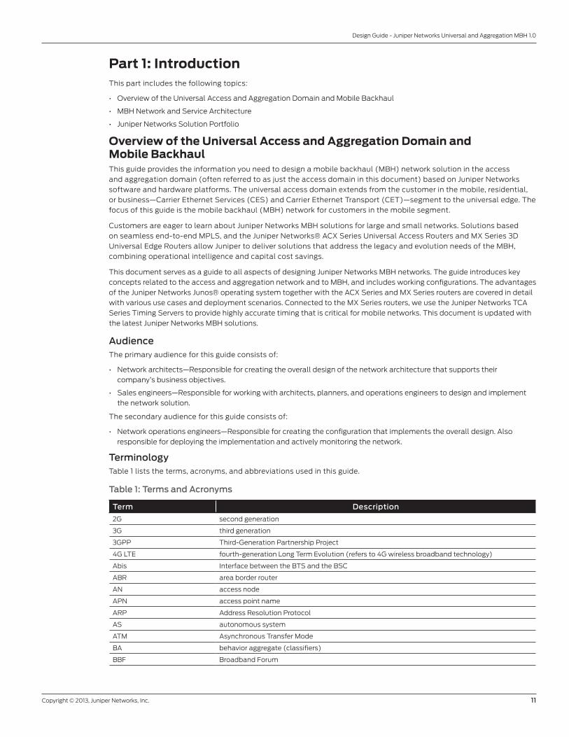
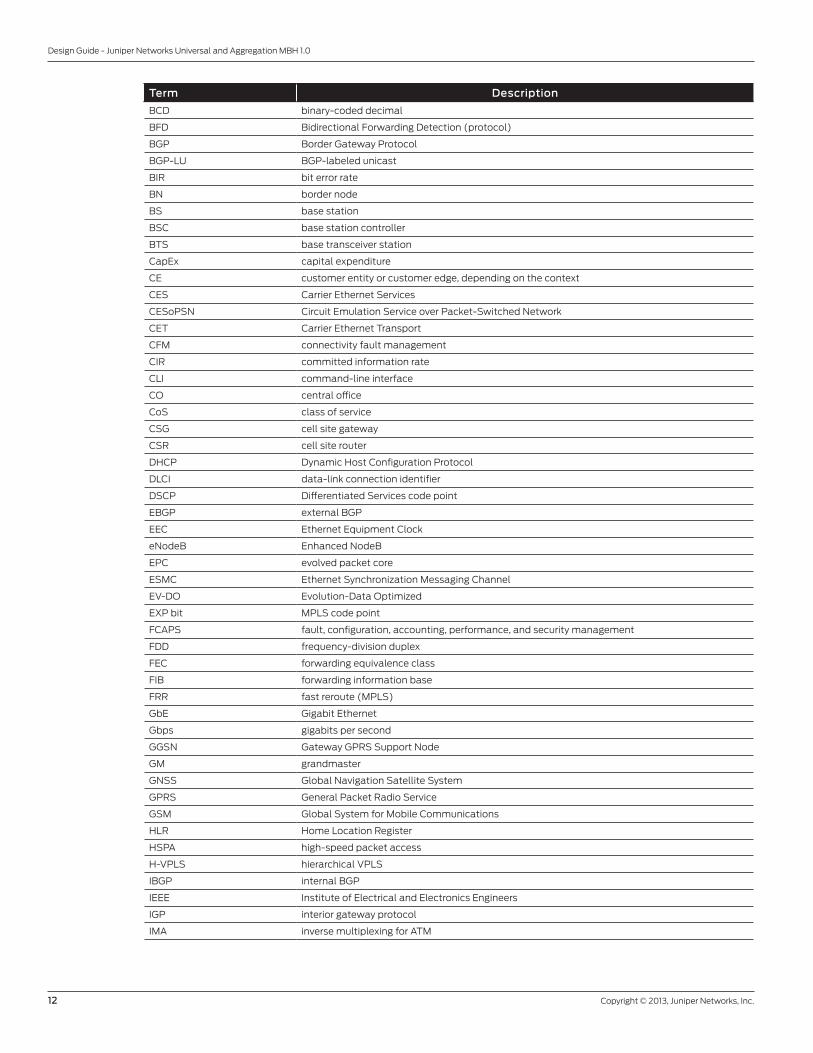
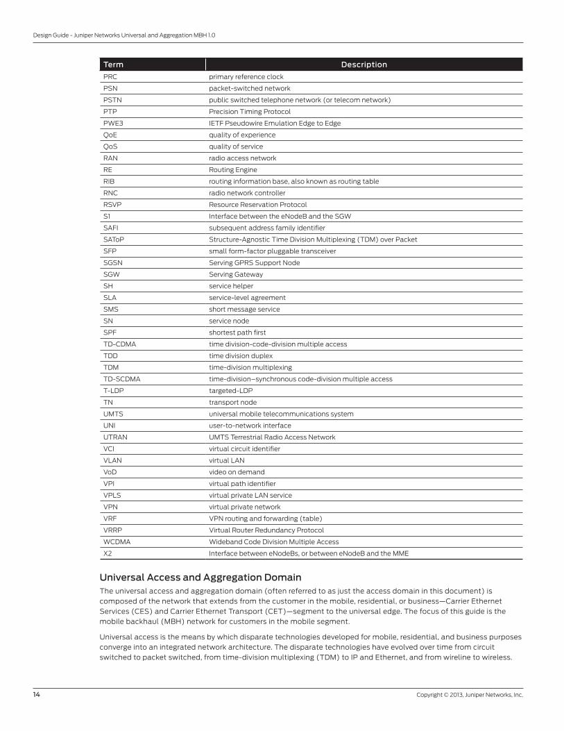
TerminologyTable 1 lists the terms, acronyms, and abbreviations used in this guide.
Table 1: Terms and Acronyms
Term Description
2G second generation
3G third generation
3GPP Third-Generation Partnership Project
4G LTE fourth-generation Long Term Evolution (refers to 4G wireless broadband technology)
Abis Interface between the BTS and the BSC
ABR area border router
AN access node
APN access point name
ARP Address Resolution Protocol
AS autonomous system
ATM Asynchronous Transfer Mode
BA behavior aggregate (classifiers)
BBF Broadband Forum
12 Copyright © 2013, Juniper Networks, Inc.
Design Guide - Juniper Networks Universal and Aggregation MBH 1.0
Term Description
BCD binary-coded decimal
BFD Bidirectional Forwarding Detection (protocol)
BGP Border Gateway Protocol
BGP-LU BGP-labeled unicast
BIR bit error rate
BN border node
BS base station
BSC base station controller
BTS base transceiver station
CapEx capital expenditure
CE customer entity or customer edge, depending on the context
CES Carrier Ethernet Services
CESoPSN Circuit Emulation Service over Packet-Switched Network
CET Carrier Ethernet Transport
CFM connectivity fault management
CIR committed information rate
CLI command-line interface
CO central office
CoS class of service
CSG cell site gateway
CSR cell site router
DHCP Dynamic Host Configuration Protocol
DLCI data-link connection identifier
DSCP Differentiated Services code point
EBGP external BGP
EEC Ethernet Equipment Clock
eNodeB Enhanced NodeB
EPC evolved packet core
ESMC Ethernet Synchronization Messaging Channel
EV-DO Evolution-Data Optimized
EXP bit MPLS code point
FCAPS fault, configuration, accounting, performance, and security management
FDD frequency-division duplex
FEC forwarding equivalence class
FIB forwarding information base
FRR fast reroute (MPLS)
GbE Gigabit Ethernet
Gbps gigabits per second
GGSN Gateway GPRS Support Node
GM grandmaster
GNSS Global Navigation Satellite System
GPRS General Packet Radio Service
GSM Global System for Mobile Communications
HLR Home Location Register
HSPA high-speed packet access
H-VPLS hierarchical VPLS
IBGP internal BGP
IEEE Institute of Electrical and Electronics Engineers
IGP interior gateway protocol
IMA inverse multiplexing for ATM

Copyright © 2013, Juniper Networks, Inc. 13
Design Guide - Juniper Networks Universal and Aggregation MBH 1.0
Term Description
IP Internet Protocol
IS-IS Intermediate system-to-Intermediate system
ISSU unified in-service software upgrade (unified ISSU)
ITU International Telecommunication Union
Iub Interface UMTS branch—Interface between the RNC and the Node B
LAN local area network
LDP Label Distribution Protocol
LDP-DOD LDP downstream on demand
LFA loop-free alternate
L-FIB label forwarding information base
LFM link fault management
LIU line interface unit
LOL loss of light
LSA link-state advertisement
LSI label-switched interface
LSP label-switched path (MPLS)
LSR label-switched router
LTE Long Term Evolution
LTE-TDD Long Term Evolution – Time Division Duplex
MBH mobile backhaul
MC-LAG multichassis link aggregation group
MEF Metro Ethernet Forum
MF multifield (classifiers)
MME mobility management entity
MP-BGP Multiprotocol BGP
MPC mobile packet core
MPLS Multiprotocol Label Switching
MSC Mobile Switching Center
MSP managed services provider. MSP can also stand for mobile service provider.
MTTR mean-time-to-resolution
NLRI network layer reachability information
NMS network management system
NNI network-to-network interface
NSR nonstop routing
NTP Network Time Protocol
OAM Operation, Administration, and Management
OpEx operational expenditure
OS operating system
OSI Open Systems Interconnection
OSPF Open Shortest Path First
OSS/BSS operations and business support systems
PCU Packet Control Unit
PDSN packet data serving node
PDU protocol data unit
PE provider edge
PFE Packet Forwarding Engine
PGW Packet Data Network Gateway
PLR point of local repair
POP point of presence
pps packets per second
14 Copyright © 2013, Juniper Networks, Inc.
Design Guide - Juniper Networks Universal and Aggregation MBH 1.0
Term Description
PRC primary reference clock
PSN packet-switched network
PSTN public switched telephone network (or telecom network)
PTP Precision Timing Protocol
PWE3 IETF Pseudowire Emulation Edge to Edge
QoE quality of experience
QoS quality of service
RAN radio access network
RE Routing Engine
RIB routing information base, also known as routing table
RNC radio network controller
RSVP Resource Reservation Protocol
S1 Interface between the eNodeB and the SGW
SAFI subsequent address family identifier
SAToP Structure-Agnostic Time Division Multiplexing (TDM) over Packet
SFP small form-factor pluggable transceiver
SGSN Serving GPRS Support Node
SGW Serving Gateway
SH service helper
SLA service-level agreement
SMS short message service
SN service node
SPF shortest path first
TD-CDMA time division-code-division multiple access
TDD time division duplex
TDM time-division multiplexing
TD-SCDMA time-division–synchronous code-division multiple access
T-LDP targeted-LDP
TN transport node
UMTS universal mobile telecommunications system
UNI user-to-network interface
UTRAN UMTS Terrestrial Radio Access Network
VCI virtual circuit identifier
VLAN virtual LAN
VoD video on demand
VPI virtual path identifier
VPLS virtual private LAN service
VPN virtual private network
VRF VPN routing and forwarding (table)
VRRP Virtual Router Redundancy Protocol
WCDMA Wideband Code Division Multiple Access
X2 Interface between eNodeBs, or between eNodeB and the MME
Universal Access and Aggregation Domain The universal access and aggregation domain (often referred to as just the access domain in this document) is
composed of the network that extends from the customer in the mobile, residential, or business—Carrier Ethernet
Services (CES) and Carrier Ethernet Transport (CET)—segment to the universal edge. The focus of this guide is the
mobile backhaul (MBH) network for customers in the mobile segment.
Universal access is the means by which disparate technologies developed for mobile, residential, and business purposes
converge into an integrated network architecture. The disparate technologies have evolved over time from circuit
switched to packet switched, from time-division multiplexing (TDM) to IP and Ethernet, and from wireline to wireless.
Copyright © 2013, Juniper Networks, Inc. 15
Design Guide - Juniper Networks Universal and Aggregation MBH 1.0
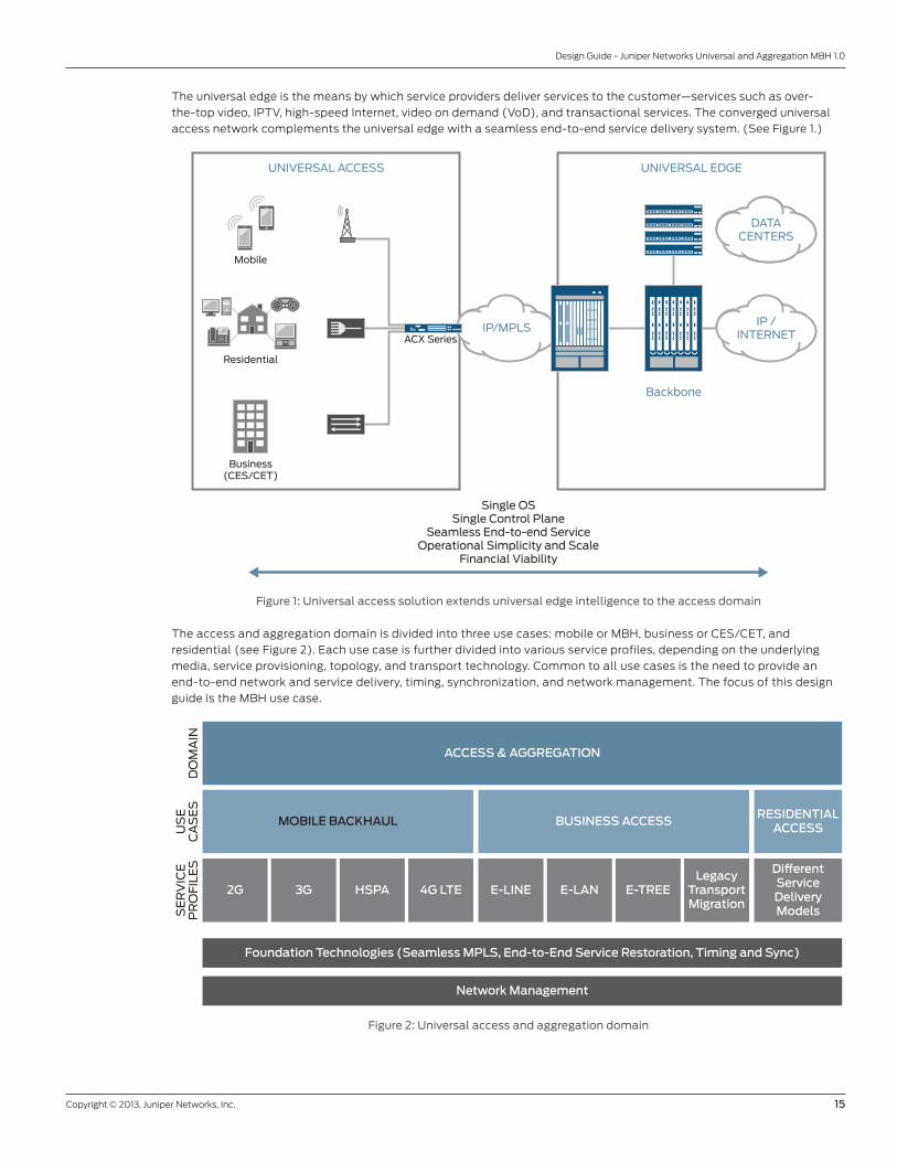
The universal edge is the means by which service providers deliver services to the customer—services such as over-
the-top video, IPTV, high-speed Internet, video on demand (VoD), and transactional services. The converged universal
access network complements the universal edge with a seamless end-to-end service delivery system. (See Figure 1.)
Single OSSingle Control Plane
Seamless End-to-end ServiceOperational Simplicity and Scale
Financial Viability
IP/MPLS
UNIVERSAL ACCESS UNIVERSAL EDGE
DATACENTERS
ACX Series
Mobile
Residential
Business(CES/CET)
Backbone
IP /INTERNET
Figure 1: Universal access solution extends universal edge intelligence to the access domain
The access and aggregation domain is divided into three use cases: mobile or MBH, business or CES/CET, and
residential (see Figure 2). Each use case is further divided into various service profiles, depending on the underlying
media, service provisioning, topology, and transport technology. Common to all use cases is the need to provide an
end-to-end network and service delivery, timing, synchronization, and network management. The focus of this design
guide is the MBH use case.
MOBILE BACKHAUL BUSINESS ACCESS
DO
MA
INU
SE
CA
SE
SS
ER
VIC
EP
RO
FIL
ES
RESIDENTIALACCESS
ACCESS & AGGREGATION
Foundation Technologies (Seamless MPLS, End-to-End Service Restoration, Timing and Sync)
Network Management
2G 3G HSPA 4G LTE E-LINE E-LAN E-TREELegacy
TransportMigration
Di�erentServiceDeliveryModels
Figure 2: Universal access and aggregation domain

16 Copyright © 2013, Juniper Networks, Inc.
Design Guide - Juniper Networks Universal and Aggregation MBH 1.0
The mobile backhaul (MBH) use case covers the technologies that must be deployed to connect mobile service
provider cell sites (base stations) to the regional mobile controller site (BSC/RNC) or mobile packet core (SGW/PGW/
MME). This use case presents complexity due to the need to support various legacy and next-generation technologies
simultaneously. Mobile service providers must continue to support legacy service profiles that enable 2G and 3G service
as well as newer and next-generation service profiles that support HSPA and 4G LTE services. Each service profile adds
potential complexity and management overhead to the network. The service provider must deal with various transports
required to support these service profiles while also working to reduce capital and operational expenditures (CapEx/
OpEx) of the MBH network. Mobile operators also seek to increase the average revenue per user through a focus on
implementing a flexible architecture that can easily change to allow for the integration of enhanced and future services.
Market SegmentsOne of the main market factors fueling a movement toward a unified and consolidated network is the rising cost of
MBH. Combine this cost increase with the ongoing exponential increase in mobile bandwidth consumption and the
introduction and rapid migration to 4G LTE, and the cost problem is further exacerbated. The subscriber’s consumption
of high-bandwidth, delay-sensitive content such as video chat, multiplayer real-time gaming, and mobile video largely
fuels the increasing demand for bandwidth. Another factor to consider is the security of the underlying infrastructure
that protects the packet core and access network. All these factors converge into a formula that makes it difficult for
mobile operators to reduce CapEx and OpEx. The increasing complexity of the network makes these goals harder to
achieve, and this makes the drive to increase average revenue per user a much more difficult proposition.
Given the challenges in this market segment, an ideal MBH network is one that is designed with a focus on consolidation
and optimization. This focus allows for more efficient installation, service provisioning, and operation of the network.
MBH Use CaseThe MBH use case described in this guide includes four service profiles for the different generations of wireless
technologies—2G, 3G, HSPA, and 4G Long Term Evolution (LTE). Each service profile represents a fundamental change
in the nature of the cellular wireless service in terms of transport technology, protocols, and access infrastructure. The
changes include a move from voice-oriented time-division multiplexing (TDM) technology toward data center-oriented
IP/Ethernet and the presence of many generations of mobile equipment, including 2G and 3G legacy as well as 4G LTE
adoption. Because the MBH solution supports any generation of mobile infrastructure, it is possible to design a smooth
migration to 4G using the information in this guide. (See Figure 3.)
Hierarchical to Flat
Hub-Spoke to Fully
Meshed
TDM/ATM to ALL-IP
INTERNET
MME
PCRF
HSS
3GPPEvolvedPacket Core
Enhanced Node B (eNodeB)
SGW PGW
IP
IP
INTERNET
PSTN
ATM/IP
TDM/ATM
IPHOSTED
SERVICES
PCRF
GGSN
SGSNGW/MSC
RNC/BSC
UTRAN
HLR
Node B Node B
OFF-NETSERVICE
ON-NETSERVICE
Figure 3: Architectural transformation of mobile service profiles
Copyright © 2013, Juniper Networks, Inc. 17
Design Guide - Juniper Networks Universal and Aggregation MBH 1.0
Problem StatementThe fundamental problem with the MBH segment is the inherent complexity introduced by the various network
elements needed to properly support the multiple generations of technology required to operate a complete MBH
network. This complexity conflicts with the provider’s ability to provide increased average revenue per user. Increasing
margin per user can be achieved by decreasing the overall cost of the network infrastructure, but how? As users
demand more bandwidth and higher quality services, the traditional answer has been “more bandwidth.” To increase
average margin per user, a service provider has to either charge more per subscriber or lower the cost of the network.
The ability to lower network cost, from an implementation, ongoing operational, and lifecycle perspective is the focus
of the MBH solution. The Juniper Networks MBH solution collapses the various MBH technologies into a converged
network designed to support the current footprint of access technologies while reducing complexity and enabling
simpler, more cost-effective network operation and management. This optimization enables easier adoption of future
technologies and new services aimed at enhancing the subscriber experience.
The service provider can achieve CapEx and OpEx reduction and facilitate higher average revenue per user by focusing
on three key areas: implementing high-performance transport, lowering the total cost of ownership of the network,
and enabling deployment flexibility. Providers have become used to the relative simplicity and reliability of legacy
TDM networks, and a packet-based network should provide similar reliability and operational simplicity and flexibility.
Additional challenges are emerging that place further emphasis on the need for high-performance transport. Flat
subscriber fees combined with an exponential increase in demand for a high-quality user experience (measured by
increased data and reliability) demand that new, more flexible business models be implemented to ensure the carrier’s
ongoing ability to provide this user experience. Lowering the total cost of ownership of the MBH network is at direct
odds with the need for high-performance transport. The operating expense associated with MBH is increasing due
not only to the growth in user data but also the increasing cost of space, power, cooling, and hardware to support new
technologies (as well as maintaining existing infrastructure to support legacy services). As more sites are provisioned,
and as the network complexity increases, the need to deploy support to a wider footprint of infrastructure further
erodes the carrier’s ability to decease the total cost of ownership of the network. Finally, deployment flexibility is a
concern as the carrier’s move more into packet-based networks. The ability of a service provider to meet strict service-
level agreements (SLAs) requires deployment of new technologies to monitor and account for network performance.
The addition of a wider array of management platforms also decreases the service provider’s ability to increase the
average margin per user of the MBH network.
The Juniper Networks universal access MBH solution is the first fully integrated end-to-end network architecture
that combines operational intelligence with capital cost savings. It is based on end-to-end IP and MPLS combined
with high-performance Juniper Networks infrastructure, which allows operators to have universal access and extend
the edge network and its capabilities to the customer, whether the customer is a cell tower, a multitenant unit, or a
residential aggregation point. This creates a seamless network architecture that is critical to delivering the benefits of
fourth-generation (4G) radio and packet core evolution with minimal truck rolls, paving the way for new revenue, new
business models, and a more flexible and efficient network.
Addressing the challenges faced in the access network by mobile service providers, this document describes the
Juniper Networks universal access MBH solution that addresses the legacy and evolution needs of the mobile network.
The solution describes design considerations and deployment choices across multiple segments of the network. It also
provides implementation guidelines to support services that can accommodate today’s mobile network needs, support
legacy services on 2G and 3G networks, and provide a migration path to LTE-based services.
Although this guide provides directions on how to design an MBH network for 2G, 3G, HSPA, and 4G LTE with concrete
examples, the major focus is the more strategic plans for a fully converged access, aggregation and edge network
infrastructure. This infrastructure provides end-to-end services to all types of consumers, including business and
residential subscribers in agreement with industry standards and recommendations that come from the Broadband
Forum (BBF), Metro Ethernet Forum (MEF), and Third-Generation Partnership Project (3GPP) working groups.
What is MBH?The backhaul is the portion of the network that connects the base station (BS) and the air interface to the base station
controllers (BSCs) and the mobile core network. The backhaul consists of a group of cell sites that are aggregated at a
series of hub sites. Figure 4 shows a high-level representation of mobile backhaul (MBH). The cell site consists of either
a single BS that is connected to the aggregation device or a collection of aggregated BSs.

18 Copyright © 2013, Juniper Networks, Inc.
Design Guide - Juniper Networks Universal and Aggregation MBH 1.0
MOBILEBACKHAUL
3G RNCNodeB
BTS
eNodeB
2G BSC
4G EPC
Figure 4: MBH
The MBH network provides transport services and connectivity between network components of the mobile operator
network. Depending on the mobile network type, the mobile network might include a number of components that
require connectivity by means of a variety of data-level and network-level protocols. (See Table 2.)
Table 2: Mobile Network Elements
Mobile Network Generation
Technology Network Element Function
2G GSM BTS Communication between air interface and the base station controller (BSC)
BSC Controls multiple base stations (BSs)
MSC Handles voice calls and short message service (SMS)
2.5G GPRS BTS Communication between air interface and BSC
SGSN Mobility management, data delivery to and from mobile user devices
GGSN Gateway to external data network packets
BSC+PCU Controls multiple BSs and processes data
3G EV-DO BTS Communication between the air interface and radio network controller (RNC)
RNC Call processing and handoffs, communication with packet data serving node (PDSN)
PDSN Gateway to external network
UTRAN NodeB Performs functions similar to base transceiver station (BTS)
RNC Performs functions similar to BSC
MSC Handles voice calls and short message service (SMS)
SGSN Mobility management, data delivery to and from mobile user devices
GGSN Gateway to external data network packets
4G LTE eNodeB Performs functions similar to BTS and radio resource management
SGW Routing and forwarding of user data, mobility anchoring
MME Tracking idle user devices, handoff management
PGW Gateway to the external data network
Types of MBHThe connectivity type offered by the backhaul network is influenced by the technology used in the radio access network
(RAN) and by factors such as the geographical location of the cell site, bandwidth requirements, and local regulations.
For instance, remote cell sites that cannot be connected over physical links use a microwave backhaul to connect to
the base station controller (BSC) and mobile core network. The amount of available frequency spectrum and spectral
efficiency of the air interface influence the bandwidth requirements of a cell site. Hence, the backhaul network can
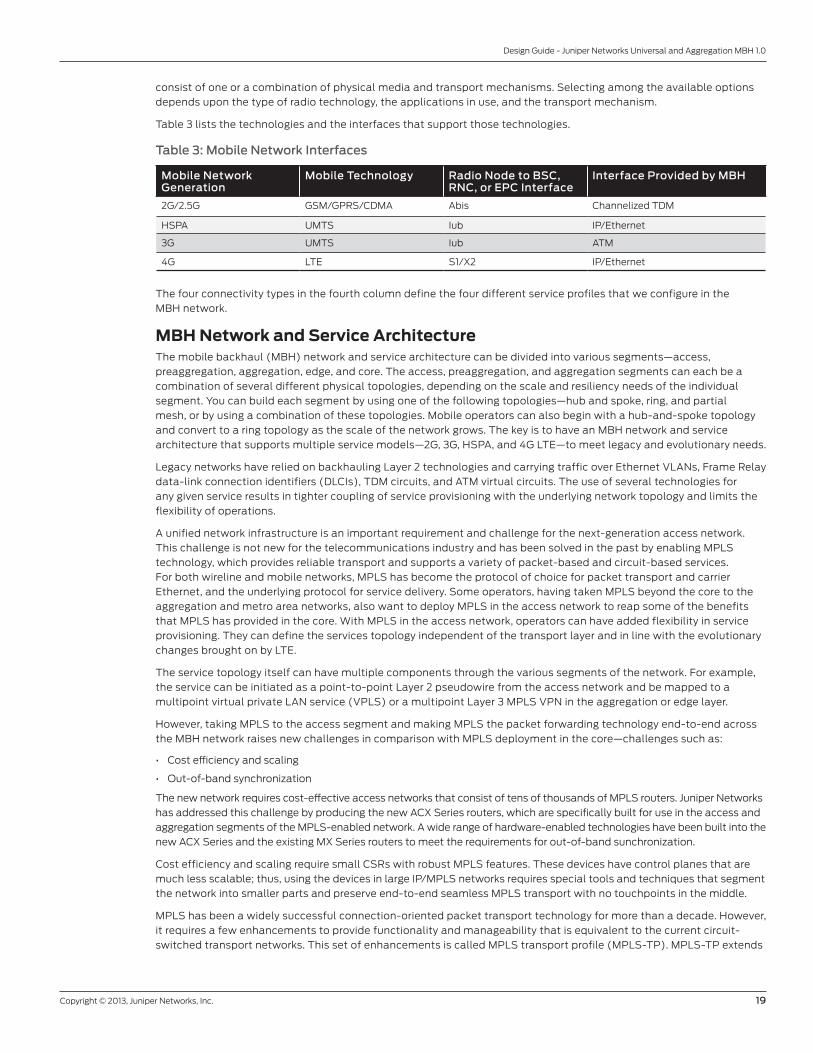
Copyright © 2013, Juniper Networks, Inc. 19
Design Guide - Juniper Networks Universal and Aggregation MBH 1.0
consist of one or a combination of physical media and transport mechanisms. Selecting among the available options
depends upon the type of radio technology, the applications in use, and the transport mechanism.
Table 3 lists the technologies and the interfaces that support those technologies.
Table 3: Mobile Network Interfaces
Mobile Network Generation
Mobile Technology Radio Node to BSC, RNC, or EPC Interface
Interface Provided by MBH
2G/2.5G GSM/GPRS/CDMA Abis Channelized TDM
HSPA UMTS Iub IP/Ethernet
3G UMTS Iub ATM
4G LTE S1/X2 IP/Ethernet
The four connectivity types in the fourth column define the four different service profiles that we configure in the
MBH network.
MBH Network and Service Architecture The mobile backhaul (MBH) network and service architecture can be divided into various segments—access,
preaggregation, aggregation, edge, and core. The access, preaggregation, and aggregation segments can each be a
combination of several different physical topologies, depending on the scale and resiliency needs of the individual
segment. You can build each segment by using one of the following topologies—hub and spoke, ring, and partial
mesh, or by using a combination of these topologies. Mobile operators can also begin with a hub-and-spoke topology
and convert to a ring topology as the scale of the network grows. The key is to have an MBH network and service
architecture that supports multiple service models—2G, 3G, HSPA, and 4G LTE—to meet legacy and evolutionary needs.
Legacy networks have relied on backhauling Layer 2 technologies and carrying traffic over Ethernet VLANs, Frame Relay
data-link connection identifiers (DLCIs), TDM circuits, and ATM virtual circuits. The use of several technologies for
any given service results in tighter coupling of service provisioning with the underlying network topology and limits the
flexibility of operations.
A unified network infrastructure is an important requirement and challenge for the next-generation access network.
This challenge is not new for the telecommunications industry and has been solved in the past by enabling MPLS
technology, which provides reliable transport and supports a variety of packet-based and circuit-based services.
For both wireline and mobile networks, MPLS has become the protocol of choice for packet transport and carrier
Ethernet, and the underlying protocol for service delivery. Some operators, having taken MPLS beyond the core to the
aggregation and metro area networks, also want to deploy MPLS in the access network to reap some of the benefits
that MPLS has provided in the core. With MPLS in the access network, operators can have added flexibility in service
provisioning. They can define the services topology independent of the transport layer and in line with the evolutionary
changes brought on by LTE.
The service topology itself can have multiple components through the various segments of the network. For example,
the service can be initiated as a point-to-point Layer 2 pseudowire from the access network and be mapped to a
multipoint virtual private LAN service (VPLS) or a multipoint Layer 3 MPLS VPN in the aggregation or edge layer.
However, taking MPLS to the access segment and making MPLS the packet forwarding technology end-to-end across
the MBH network raises new challenges in comparison with MPLS deployment in the core—challenges such as:
• Cost efficiency and scaling
• Out-of-band synchronization
The new network requires cost-effective access networks that consist of tens of thousands of MPLS routers. Juniper Networks
has addressed this challenge by producing the new ACX Series routers, which are specifically built for use in the access and
aggregation segments of the MPLS-enabled network. A wide range of hardware-enabled technologies have been built into the
new ACX Series and the existing MX Series routers to meet the requirements for out-of-band sunchronization.
Cost efficiency and scaling require small CSRs with robust MPLS features. These devices have control planes that are
much less scalable; thus, using the devices in large IP/MPLS networks requires special tools and techniques that segment
the network into smaller parts and preserve end-to-end seamless MPLS transport with no touchpoints in the middle.
MPLS has been a widely successful connection-oriented packet transport technology for more than a decade. However,
it requires a few enhancements to provide functionality and manageability that is equivalent to the current circuit-
switched transport networks. This set of enhancements is called MPLS transport profile (MPLS-TP). MPLS-TP extends

20 Copyright © 2013, Juniper Networks, Inc.
Design Guide - Juniper Networks Universal and Aggregation MBH 1.0
the already rich MPLS and Generalized MPLS (GMPLS) protocol suite to serve transport and service networks with
enhancements to the data plane, such as framing, forwarding, encapsulation, OAM, and resiliency. MPLS-TP is planned
for inclusion as part of seamless MPLS in future versions of the access and aggregation solution.
Seamless MPLS addresses the requirements for extending MPLS to the access network and significantly influences
the architectural framework for building scalable and resilient MPLS networks with a flexible services delivery model.
The topic “Seamless MPLS” describes the benefits and requirements for seamless MPLS, along with the features and
functionality supported by our Juniper Networks comprehensive MPLS portfolio, which delivers a complete and flexible
solution for MBH.
The MBH network and services architecture can be viewed in two dimensions—the infrastructure of the network and
the different layers of the network.
MBH Network InfrastructureThe first dimension of the MBH network architecture is represented by the network infrastructure, which is defined
by TR-221, Technical Specification for MPLS in the MBH Networks, of the Broadband Forum. TR-221 defines the use of
MPLS in the MBH access and aggregation network and provides solutions for the transport of traffic in 2G, 3G, HSPA,
and 4G LTE mobile networks. The main elements of the infrastructure are the segments that appear in Figure 5:
• Access—includes CSRs
• Preaggregation
• Aggregation
• Core—includes service edge and remote service edge routers
ServiceEdgeCSRs
RemoteService
Edge
RAN ACCESS CORE NETWORKPRE-AGGREGATION
AGGREGATION
MPLS
4G EPC
MME
SGW/PGW
HSS
PCRF
Figure 5: MBH network infrastructure
This document describes deployment scenarios for the access, preaggregation, aggregation, and core segments. The
core segment is, of course, an essential part of the solution. The RAN and evolved packet core (EPC) segments are
included in Figure 5 for completeness. Our solution leverages the MPLS core and extends core capabilities into the
access and aggregation segments. However, in most cases, the operator already has an IP and MPLS core, so this
document does not describe the details of the core segment. It does, instead, describe some functional requirements
for the provider edge (PE) service routers, which are a part of the core segment.
Access Segment
The access segment consists of the CSR, which is typically deployed at the cell site and connects the BS to the packet
network. Several CSRs can be connected in a ring or hub-and-spoke topology to the upstream preaggregation and
aggregation routers. Key requirements of a CSR include:
• Support for TDM and Ethernet interfaces to meet multigeneration needs (2G, 3G, HSPA, and 4G LTE)
• Timing and synchronization support for voice and TDM traffic
• Performance and bandwidth to meet growing service needs
• Software features to deliver an enhanced quality of experience (QoE)—class of service, network resiliency, and operation,
administration, and management (OAM)
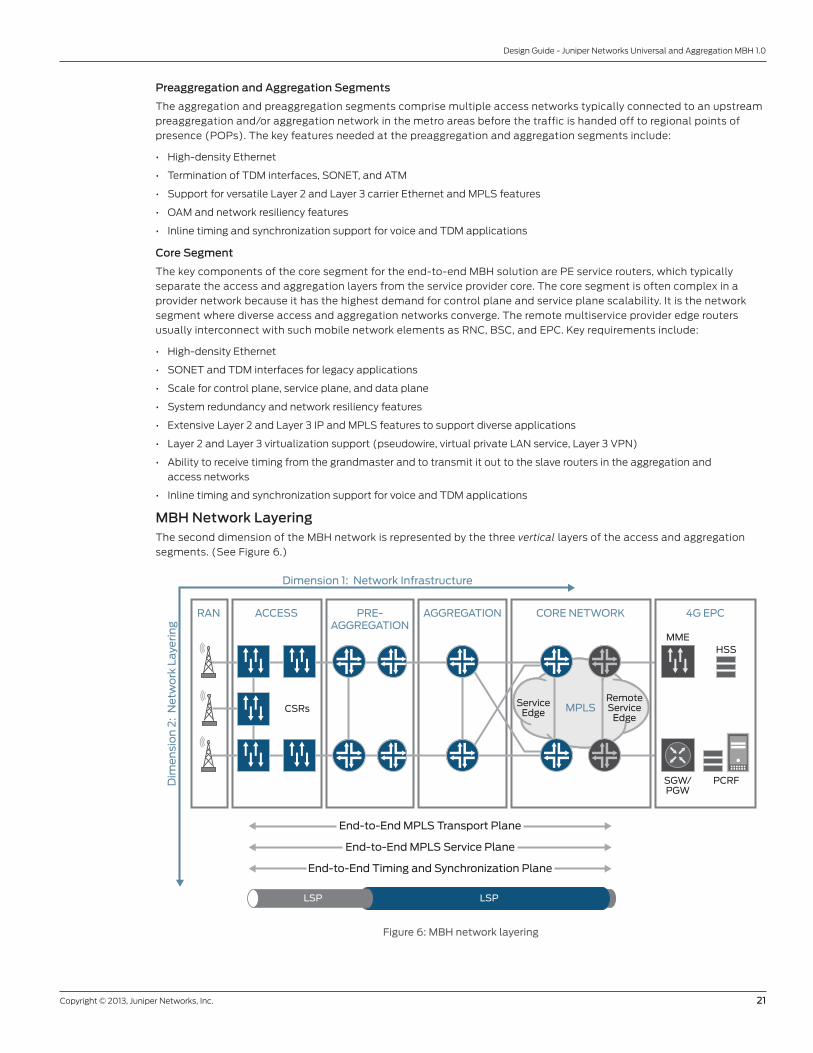
Copyright © 2013, Juniper Networks, Inc. 21
Design Guide - Juniper Networks Universal and Aggregation MBH 1.0
Preaggregation and Aggregation Segments
The aggregation and preaggregation segments comprise multiple access networks typically connected to an upstream
preaggregation and/or aggregation network in the metro areas before the traffic is handed off to regional points of
presence (POPs). The key features needed at the preaggregation and aggregation segments include:
• High-density Ethernet
• Termination of TDM interfaces, SONET, and ATM
• Support for versatile Layer 2 and Layer 3 carrier Ethernet and MPLS features
• OAM and network resiliency features
• Inline timing and synchronization support for voice and TDM applications
Core Segment
The key components of the core segment for the end-to-end MBH solution are PE service routers, which typically
separate the access and aggregation layers from the service provider core. The core segment is often complex in a
provider network because it has the highest demand for control plane and service plane scalability. It is the network
segment where diverse access and aggregation networks converge. The remote multiservice provider edge routers
usually interconnect with such mobile network elements as RNC, BSC, and EPC. Key requirements include:
• High-density Ethernet
• SONET and TDM interfaces for legacy applications
• Scale for control plane, service plane, and data plane
• System redundancy and network resiliency features
• Extensive Layer 2 and Layer 3 IP and MPLS features to support diverse applications
• Layer 2 and Layer 3 virtualization support (pseudowire, virtual private LAN service, Layer 3 VPN)
• Ability to receive timing from the grandmaster and to transmit it out to the slave routers in the aggregation and
access networks
• Inline timing and synchronization support for voice and TDM applications
MBH Network Layering The second dimension of the MBH network is represented by the three vertical layers of the access and aggregation
segments. (See Figure 6.)
Dimension 1: Network Infrastructure
Dim
en
sio
n 2
: N
etw
ork
La
yeri
ng
LSPLSP
ServiceEdgeCSRs
RemoteService
Edge
RAN ACCESS CORE NETWORKPRE-AGGREGATION
AGGREGATION
MPLS
End-to-End Timing and Synchronization Plane
End-to-End MPLS Transport Plane
End-to-End MPLS Service Plane
4G EPC
MME
SGW/PGW
HSS
PCRF
Figure 6: MBH network layering

22 Copyright © 2013, Juniper Networks, Inc.
Design Guide - Juniper Networks Universal and Aggregation MBH 1.0
The three layers of the MBH network infrastructure include:
• End-to-end timing and synchronization
• End-to-end MPLS-based services
• End-to-end MPLS transport
End-to-End Timing and Synchronization
Typically, mobile networks utilize SONET or SDH technologies to backhaul voice and data traffic, and use native support
for frequency of SONET or SDH to synchronize their radio network. Unless you synchronize the two ends of a circuit, the
target device cannot decode the data encoded by the source device. When you emulate the circuit over an IP-based
or packet-based network, the continuity of the circuit clock is lost. The fundamental difference between typical native
support for synchronization and an emulated circuit in the IP-based or packet-based network is that typical native
support is synchronous while the emulated circuit has traditionally been asynchronous. This disparity means that a
timing and synchronization solution must be employed when performing circuit emulation over the MPLS backbone.
Clock synchronization in an MBH network is an essential requirement for handoff support, voice quality, and low
interference. Loss of timing synchronization can result in poor user experience, service disruptions, and waste of
frequency spectrum. A base station clock needs to be within certain limits of the central radio controller to ensure
seamless handover between different base stations. Wireless technologies based on frequency-division duplex
(FDD)—such as 2G GSM or 3G UMTS, WiMAX FDD, LTE-FDD, and W-CDMA—require only frequency synchronization
to the reference clock. However, wireless technologies based on time-division duplex (TDD)—such as TD-CDMA/
CDMA2000, TD-SCDMA, and LTE-TDD—require both frequency and time (phase and time-of-day) synchronization to
the reference clock.
There are multiple ways of distributing the timing information across the MBH network:
• Traditional TDM-based timing distribution
• IEEE 1588v2 Precision Timing Protocol (PTP)
• Synchronous Ethernet over the physical layer
• Network Time Protocol (NTP)v3 and NTPv4
• GPS or BITS that is external to the IP-packet based network
Juniper Networks supports multiple timing synchronization options because a single timing solution does not fit all
network types or requirements. For synchronization distribution across the MBH network, we use two main methods:
physical layer-based Synchronous Ethernet (G.8261, and so on) and packet-based Precision Timing Protocol (PTP),
standardized in IEEE 1588-2008. Both methods are complementary to each other and are a versatile fit for IP/
Ethernet-based MBH because they are topology agnostic and support frequency (Synchronous Ethernet) and phase
(IEEE 1588v2). In addition, when applying class-of-service (CoS) rules, we classify packets carrying timing information
into the high-priority, low-latency queue.
End-to-End MPLS-Based Services
Many types of network services are based on MPLS VPNs, which offer end-to-end connectivity between sites over a
shared IP/MPLS network.
VPNs are classified as either Layer 2 or Layer 3. In a Layer 2 VPN, the provider network offers only transport services
between customer edge (CE) devices over the VPN. The routing and peering take place between CEs; the IP addressing
and routing of customer traffic are passed over Layer 2 and are encapsulated, becoming essentially transparent to the
provider network. This type of VPN is also known as the overlay model. Legacy Layer 2 VPNs include Frame Relay, ATM,
or time-division multiplexing (TDM) networks. Modern Layer 2 VPNs use IP and MPLS across the provider network.
The simplest example of a Layer 2 VPN, which is widely used in the Juniper Networks MBH solution, is a pseudowire
connection. The pseudowire connection begins and terminates at the physical port or logical interface where traffic
enters the PE router. Within each Layer 2 VPN or service, we configure several pseudowires to carry Layer 2 traffic. The
IETF Pseudowire Emulation Edge to Edge (PWE3) standards define how Layer 2 traffic is carried across the network.
In contrast, we configure Layer 3 VPNs with peering between CE and PE devices, and the carrier or provider network
routing customer traffic over the VPN. The provider network can present each customer’s logical network with route
distribution and transport services, which we refer to as the peer model.
One problem in a traditional carrier network, which includes multiple network segments such as access, aggregation,
and core, is the number of touchpoints that you need to provision to activate new services. This introduces additional
and unnecessary complexity into an already complex network environment. In the traditional multisegment network,
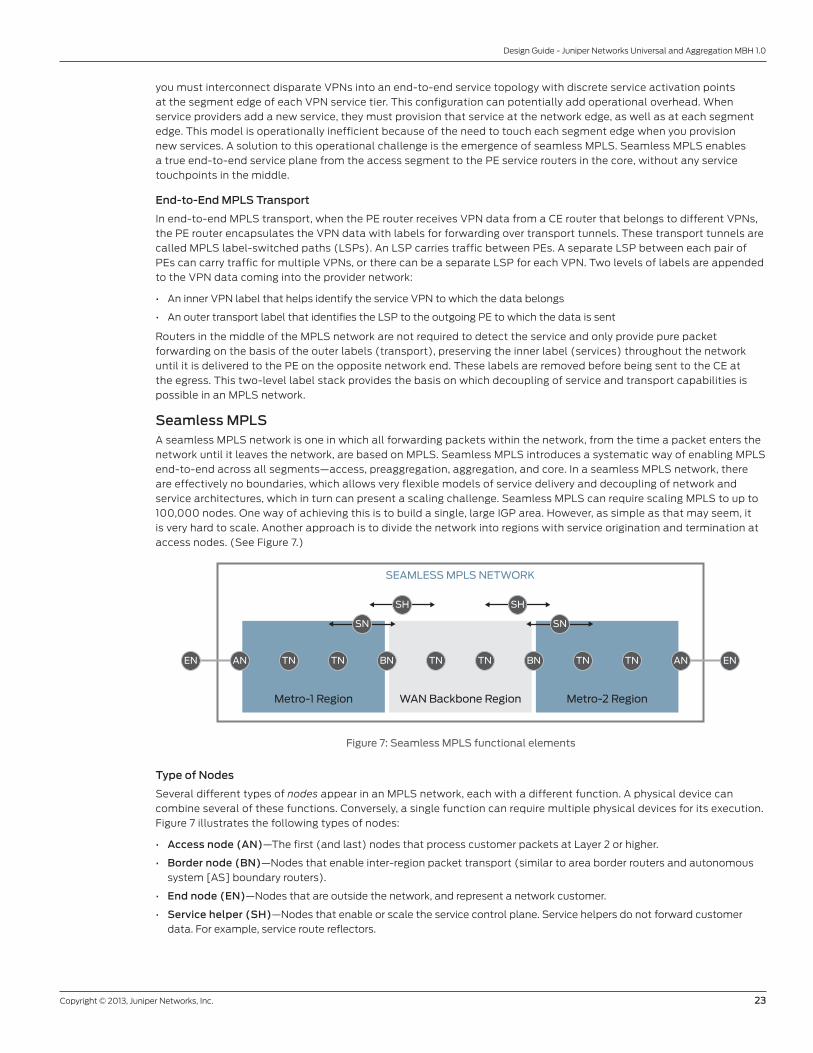
Copyright © 2013, Juniper Networks, Inc. 23
Design Guide - Juniper Networks Universal and Aggregation MBH 1.0
you must interconnect disparate VPNs into an end-to-end service topology with discrete service activation points
at the segment edge of each VPN service tier. This configuration can potentially add operational overhead. When
service providers add a new service, they must provision that service at the network edge, as well as at each segment
edge. This model is operationally inefficient because of the need to touch each segment edge when you provision
new services. A solution to this operational challenge is the emergence of seamless MPLS. Seamless MPLS enables
a true end-to-end service plane from the access segment to the PE service routers in the core, without any service
touchpoints in the middle.
End-to-End MPLS Transport
In end-to-end MPLS transport, when the PE router receives VPN data from a CE router that belongs to different VPNs,
the PE router encapsulates the VPN data with labels for forwarding over transport tunnels. These transport tunnels are
called MPLS label-switched paths (LSPs). An LSP carries traffic between PEs. A separate LSP between each pair of
PEs can carry traffic for multiple VPNs, or there can be a separate LSP for each VPN. Two levels of labels are appended
to the VPN data coming into the provider network:
• An inner VPN label that helps identify the service VPN to which the data belongs
• An outer transport label that identifies the LSP to the outgoing PE to which the data is sent
Routers in the middle of the MPLS network are not required to detect the service and only provide pure packet
forwarding on the basis of the outer labels (transport), preserving the inner label (services) throughout the network
until it is delivered to the PE on the opposite network end. These labels are removed before being sent to the CE at
the egress. This two-level label stack provides the basis on which decoupling of service and transport capabilities is
possible in an MPLS network.
Seamless MPLSA seamless MPLS network is one in which all forwarding packets within the network, from the time a packet enters the
network until it leaves the network, are based on MPLS. Seamless MPLS introduces a systematic way of enabling MPLS
end-to-end across all segments—access, preaggregation, aggregation, and core. In a seamless MPLS network, there
are effectively no boundaries, which allows very flexible models of service delivery and decoupling of network and
service architectures, which in turn can present a scaling challenge. Seamless MPLS can require scaling MPLS to up to
100,000 nodes. One way of achieving this is to build a single, large IGP area. However, as simple as that may seem, it
is very hard to scale. Another approach is to divide the network into regions with service origination and termination at
access nodes. (See Figure 7.)
EN EN
WAN Backbone Region Metro-2 RegionMetro-1 Region
BN BNTN TN TN TNTN TN ANAN
SEAMLESS MPLS NETWORK
SH SH
SN SN
Figure 7: Seamless MPLS functional elements
Type of Nodes
Several different types of nodes appear in an MPLS network, each with a different function. A physical device can
combine several of these functions. Conversely, a single function can require multiple physical devices for its execution.
Figure 7 illustrates the following types of nodes:
• Access node (AN)—The first (and last) nodes that process customer packets at Layer 2 or higher.
• Border node (BN)—Nodes that enable inter-region packet transport (similar to area border routers and autonomous
system [AS] boundary routers).
• End node (EN)—Nodes that are outside the network, and represent a network customer.
• Service helper (SH)—Nodes that enable or scale the service control plane. Service helpers do not forward customer
data. For example, service route reflectors.
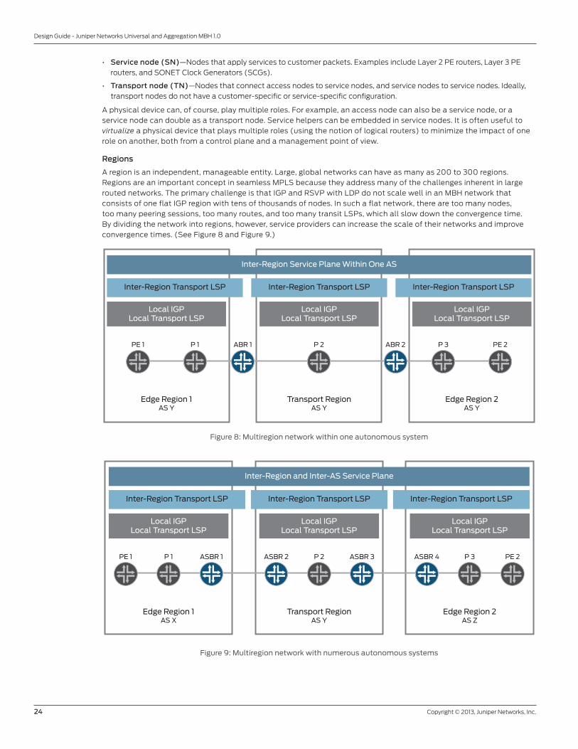
24 Copyright © 2013, Juniper Networks, Inc.
Design Guide - Juniper Networks Universal and Aggregation MBH 1.0
• Service node (SN)—Nodes that apply services to customer packets. Examples include Layer 2 PE routers, Layer 3 PE
routers, and SONET Clock Generators (SCGs).
• Transport node (TN)—Nodes that connect access nodes to service nodes, and service nodes to service nodes. Ideally,
transport nodes do not have a customer-specific or service-specific configuration.
A physical device can, of course, play multiple roles. For example, an access node can also be a service node, or a
service node can double as a transport node. Service helpers can be embedded in service nodes. It is often useful to
virtualize a physical device that plays multiple roles (using the notion of logical routers) to minimize the impact of one
role on another, both from a control plane and a management point of view.
Regions
A region is an independent, manageable entity. Large, global networks can have as many as 200 to 300 regions.
Regions are an important concept in seamless MPLS because they address many of the challenges inherent in large
routed networks. The primary challenge is that IGP and RSVP with LDP do not scale well in an MBH network that
consists of one flat IGP region with tens of thousands of nodes. In such a flat network, there are too many nodes,
too many peering sessions, too many routes, and too many transit LSPs, which all slow down the convergence time.
By dividing the network into regions, however, service providers can increase the scale of their networks and improve
convergence times. (See Figure 8 and Figure 9.)
Inter-Region Transport LSP Inter-Region Transport LSP Inter-Region Transport LSP
Inter-Region Service Plane Within One AS
ABR 1 P 2
Transport RegionAS Y
Edge Region 2AS Y
Edge Region 1AS Y
ABR 2PE 1 P 1 PE 2P 3
Local IGPLocal Transport LSP
Local IGPLocal Transport LSP
Local IGPLocal Transport LSP
Figure 8: Multiregion network within one autonomous system
Inter-Region Transport LSP Inter-Region Transport LSP Inter-Region Transport LSP
Inter-Region and Inter-AS Service Plane
Transport RegionAS Y
Edge Region 2AS Z
Edge Region 1AS X
ASBR 4 P 3 PE 2PE 1 ASBR 2P 1 ASBR 1 P 2 ASBR 3
Local IGPLocal Transport LSP
Local IGPLocal Transport LSP
Local IGPLocal Transport LSP
Figure 9: Multiregion network with numerous autonomous systems

Copyright © 2013, Juniper Networks, Inc. 25
Design Guide - Juniper Networks Universal and Aggregation MBH 1.0
Figure 8 and Figure 9 show two examples of inter-region networks consisting of three regions covering the edge and
transport regions—edge regions 1 and 2, and the transport region. This approach segments the end-to-end connectivity
problem into inter-region and intraregion connectivity and introduces a hierarchical topology that is a key component
in the design of seamless MPLS, allowing network to scale well. (For the benefits of seamless MPLS, see the topic
“Solution Value Proposition.”) From the control plane perspective, regions can be of different types:
• Interior gateway protocol (IGP) region—Traditional multi-area/multilevel IGP design, with multiple area border routers
(ABRs) connecting the areas and regions
• IGP instance—Separate IGP instance for each region, with multiple border routers connecting the regions
• BGP AS—Separate BGP AS for each area, with multiple pairs of boundary routers connecting the regions
The characteristics of a multiregion network are quite similar to a multi-area OSPF network, multilevel IS-IS network, or
BGP AS, but the regions do not exchange routing information as would a typical area or level. IGP routing information,
LDP signaling, or RSVP signaling is not exchanged between regions.
End-to-End Hierarchical LSP
Although regions add scale, they establish explicit boundaries and cut end-to-end transport into a few separate
LSPs per region. To alleviate this problem, LSPs can be stitched between regions, extending the MPLS network over
multiple regions in the MBH network. These LSPs are hierarchical end-to-end LSPs. Inside each region, hierarchical
LSPs are built on the metrics of existing control plane functionality using the OSPF or IS-IS and RSVP or LDP protocols.
Meanwhile all inter-region control plane information is shared with BGP-labeled unicast (BGP-LU). Sharing allows the
distribution of labeled routes for the service node’s loopback interface across all regions, providing end-to-end MPLS
tunneling. Transit routers within each region are not required to detect or participate in BGP-LU , which is one of the
reasons BGP-LU scales so well.
Decoupling Services and Transport with Seamless MPLS
The following 4G LTE and HSPA scenarios illustrate how the typical MBH architecture fits seamless MPLS in terms of
defined functions, transport LSPs, and decoupling of the services plane from the underlying topology and transport plane.
Figure 10 shows the functional roles of different network nodes for a 4G LTE deployment scenario.
ServiceEdgeCSRs
RemoteService
Edge
RAN ACCESS PRE-AGGREGATION
AGGREGATION 4G EPC
MPLS
MME
SGW/PGW
HSS
PCRF
EN
ENSH
BN BNTN
TN
SN
SH
BN
AN
SN
L3 VPN
Seamless MPLS Network of a Mobile Operator
SH
BN
L3 VPNLSPLSP
CORE NETWORK
Figure 10: Seamless MPLS functions in a 4G LTE backhaul network
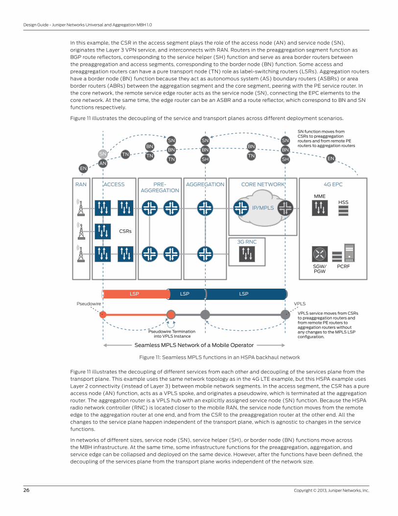
26 Copyright © 2013, Juniper Networks, Inc.
Design Guide - Juniper Networks Universal and Aggregation MBH 1.0
In this example, the CSR in the access segment plays the role of the access node (AN) and service node (SN),
originates the Layer 3 VPN service, and interconnects with RAN. Routers in the preaggregation segment function as
BGP route reflectors, corresponding to the service helper (SH) function and serve as area border routers between
the preaggregation and access segments, corresponding to the border node (BN) function. Some access and
preaggregation routers can have a pure transport node (TN) role as label-switching routers (LSRs). Aggregation routers
have a border node (BN) function because they act as autonomous system (AS) boundary routers (ASBRs) or area
border routers (ABRs) between the aggregation segment and the core segment, peering with the PE service router. In
the core network, the remote service edge router acts as the service node (SN), connecting the EPC elements to the
core network. At the same time, the edge router can be an ASBR and a route reflector, which correspond to BN and SN
functions respectively.
Figure 11 illustrates the decoupling of the service and transport planes across different deployment scenarios.
CSRs
RAN ACCESS PRE-AGGREGATION
IP/MPLS
Seamless MPLS Network of a Mobile Operator
EN
ENTN
BN
TN
BN
TN
SN
SH
BN
SN
SH
BN
SN
TN
BN
AN
SN
AGGREGATION CORE NETWORK
3G RNC
4G EPC
MME
SGW/PGW
HSS
PCRF
LSPLSPLSP
Pseudowire Termination into VPLS Instance
SN function moves fromCSRs to preaggregation routers and from remote PErouters to aggregation routers
VPLS service moves from CSRsto preaggregation routers and from remote PE routers toaggregation routers withoutany changes to the MPLS LSPconfiguration.
VPLSPseudowire
Figure 11: Seamless MPLS functions in an HSPA backhaul network
Figure 11 illustrates the decoupling of different services from each other and decoupling of the services plane from the
transport plane. This example uses the same network topology as in the 4G LTE example, but this HSPA example uses
Layer 2 connectivity (instead of Layer 3) between mobile network segments. In the access segment, the CSR has a pure
access node (AN) function, acts as a VPLS spoke, and originates a pseudowire, which is terminated at the aggregation
router. The aggregation router is a VPLS hub with an explicitly assigned service node (SN) function. Because the HSPA
radio network controller (RNC) is located closer to the mobile RAN, the service node function moves from the remote
edge to the aggregation router at one end, and from the CSR to the preaggregation router at the other end. All the
changes to the service plane happen independent of the transport plane, which is agnostic to changes in the service
functions.
In networks of different sizes, service node (SN), service helper (SH), or border node (BN) functions move across
the MBH infrastructure. At the same time, some infrastructure functions for the preaggregation, aggregation, and
service edge can be collapsed and deployed on the same device. However, after the functions have been defined, the
decoupling of the services plane from the transport plane works independent of the network size.

Copyright © 2013, Juniper Networks, Inc. 27
Design Guide - Juniper Networks Universal and Aggregation MBH 1.0
Mobile Service ProfilesPositioned in the access and aggregation domain, the MBH use case described in this guide includes four service
profiles for the different generations of wireless technologies—2G, 3G, HSPA, and 4G LTE. Each service profile includes
examples of a variety of deployment scenarios. (See Figure 12.)
Syn
cE
158
8 v
2
Rin
g T
op
olo
gy
Hu
b a
nd
Sp
oke
USE CASE SERVICEPROFILE
Deployment Scenarios
SYNC & TIMESERVICES IP/MPLSTRANSPORT
TOPOLOGY
IS-I
S, R
SV
P, B
GP
-LU
, LD
P-D
OD
SAToP
OS
PF,
RS
VP
(A
gg
reg
ati
on
an
d C
ore
),
BG
P-L
U, L
DP
-DO
D, O
SP
F L
FA
MBH
ATMPseudowire
CESoPSN
H-VPLS
L3 VPN withPseudowire
in Access
L3 VPN
3G
2G
HSPA
4G LTE
Figure 12: MBH service profiles and deployment scenarios
The deployment scenarios for each service profile include different services. Common to all service profiles are the IP/
MPLS transport, synchronization and timing, and topology elements. That is, all service profiles and services are based
on a common IP/MPLS transport infrastructure, common synchronization and timing, and a common network topology.
The IP/MPLS transport infrastructure can be IS-IS or OSPF-based, synchronization can be Synchronous Ethernet, IEEE
1588v2, or a combination of the two, and the topology can be ring or hub and spoke, depending on the example.
The deployment scenarios represent separate building blocks that can be deployed alone or combined with each other.
2G Service Profile
The 2G service profile examples include the following features:
• End-to-end TDM Circuit Emulation Service over Packet-Switched Network (CESoPSN)—A CESoPSN bundle represents
an IP circuit emulation flow. With CESoPSN bundles, you can group multiple DS0s on one IP circuit, and you can have
more than one circuit emulation IP flow created from a single physical interface. For example, some DS0 channels
from a T1 interface can go in an IP flow to destination A, and other DS0 channels from that same T1 interface can go to
destination B. This feature allows for payload optimization. CESoPSN bundles comply with RFC 5086, Structure-Aware
Time Division Multiplexed (TDM) Circuit Emulation Service over Packet Switched Network (CESoPSN).
• Structure-Agnostic Time Division Multiplexing (TDM) over Packet (SAToP)—SAToP bundles use a standards-based
transport mechanism for T1/E1 circuits that allows them to interoperate with other SAToP-compliant equipment. SAToP
bundles comply with RFC 4553 to provide pseudowire encapsulation. Pseudowire Emulation Edge to Edge (PWE3)
for TDM bit streams (T1, E1, T3, E3) disregards any structure that might be imposed on these streams, in particular the
structure imposed by the standard TDM framing.
3G Service Profile
The 3G universal mobile telecommunications system (UMTS) service profile example includes edge-to-edge
Asynchronous Transfer Mode (ATM) pseudowires as described in RFC 4717. ATM pseudowires (a simulated wired
connection that emulates a dedicated end-to-end wire) are used to carry ATM cells over an MPLS network, enabling
service providers to offer emulated ATM services over existing MPLS networks.
HSPA Service Profile
The HSPA service profile examples include a combination of a Layer 2 VPN signaled with LDP (RFC 4905) and LDP-
signaled virtual private LAN service (VPLS). A Layer 2 VPN enables transport of the protocol data unit (PDU) of Layer
2 protocols such as Frame Relay, ATM AAL5, and Ethernet, and providing a circuit emulation service across an MPLS
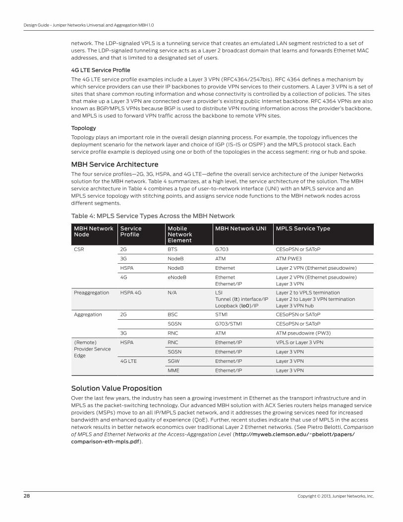
28 Copyright © 2013, Juniper Networks, Inc.
Design Guide - Juniper Networks Universal and Aggregation MBH 1.0
network. The LDP-signaled VPLS is a tunneling service that creates an emulated LAN segment restricted to a set of
users. The LDP-signaled tunneling service acts as a Layer 2 broadcast domain that learns and forwards Ethernet MAC
addresses, and that is limited to a designated set of users.
4G LTE Service Profile
The 4G LTE service profile examples include a Layer 3 VPN (RFC4364/2547bis). RFC 4364 defines a mechanism by
which service providers can use their IP backbones to provide VPN services to their customers. A Layer 3 VPN is a set of
sites that share common routing information and whose connectivity is controlled by a collection of policies. The sites
that make up a Layer 3 VPN are connected over a provider’s existing public Internet backbone. RFC 4364 VPNs are also
known as BGP/MPLS VPNs because BGP is used to distribute VPN routing information across the provider’s backbone,
and MPLS is used to forward VPN traffic across the backbone to remote VPN sites.
Topology
Topology plays an important role in the overall design planning process. For example, the topology influences the
deployment scenario for the network layer and choice of IGP (IS-IS or OSPF) and the MPLS protocol stack. Each
service profile example is deployed using one or both of the topologies in the access segment: ring or hub and spoke.
MBH Service Architecture The four service profiles—2G, 3G, HSPA, and 4G LTE—define the overall service architecture of the Juniper Networks
solution for the MBH network. Table 4 summarizes, at a high level, the service architecture of the solution. The MBH
service architecture in Table 4 combines a type of user-to-network interface (UNI) with an MPLS service and an
MPLS service topology with stitching points, and assigns service node functions to the MBH network nodes across
different segments.
Table 4: MPLS Service Types Across the MBH Network
MBH NetworkNode
ServiceProfile
Mobile NetworkElement
MBH Network UNI MPLS Service Type
CSR 2G BTS G.703 CESoPSN or SAToP
3G NodeB ATM ATM PWE3
HSPA NodeB Ethernet Layer 2 VPN (Ethernet pseudowire)
4G eNodeB EthernetEthernet/IP
Layer 2 VPN (Ethernet pseudowire)Layer 3 VPN
Preaggregation HSPA 4G N/A LSITunnel (lt) interface/IPLoopback (lo0)/IP
Layer 2 to VPLS terminationLayer 2 to Layer 3 VPN terminationLayer 3 VPN hub
Aggregation 2G BSC STM1 CESoPSN or SAToP
SGSN G703/STM1 CESoPSN or SAToP
3G RNC ATM ATM pseudowire (PW3)
(Remote)Provider ServiceEdge
HSPA RNC Ethernet/IP VPLS or Layer 3 VPN
SGSN Ethernet/IP Layer 3 VPN
4G LTE SGW Ethernet/IP Layer 3 VPN
MME Ethernet/IP Layer 3 VPN
Solution Value PropositionOver the last few years, the industry has seen a growing investment in Ethernet as the transport infrastructure and in
MPLS as the packet-switching technology. Our advanced MBH solution with ACX Series routers helps managed service
providers (MSPs) move to an all IP/MPLS packet network, and it addresses the growing services need for increased
bandwidth and enhanced quality of experience (QoE). Further, recent studies indicate that use of MPLS in the access
network results in better network economics over traditional Layer 2 Ethernet networks. (See Pietro Belotti, Comparison
of MPLS and Ethernet Networks at the Access-Aggregation Level (http://myweb.clemson.edu/~pbelott/papers/comparison-eth-mpls.pdf).

Copyright © 2013, Juniper Networks, Inc. 29
Design Guide - Juniper Networks Universal and Aggregation MBH 1.0
Juniper Networks provides an industry-leading solution to deliver a services architecture that moves MPLS from the
core and aggregation layers into the access layer, providing the necessary functionality and performance needed to
build highly resilient, large-scale, modern day networks.
The key benefits of building an end-to-end MPLS network for wireless services include:
• Supporting multiple types of transport infrastructure—MPLS can efficiently carry both packet and nonpacket application
traffic over a hybrid underlying infrastructure that includes TDM, ATM, and Ethernet.
• Decoupling the underlying infrastructure—Services can be initiated as MPLS pseudowires or MPLS Layer 3 VPNs at
the cell site and can be flexibly mapped to MPLS services at the aggregation and edge nodes farther upstream in the
network. In contrast, traditional networks have relied on backhauling Layer 2 technologies and carrying traffic over
Ethernet VLANs, Frame Relay data-link connection identifier (DLCI), or ATM virtual circuits. This approach of dealing
with several technologies for any given service has resulted in tighter coupling of service provisioning to the underlying
topology and limited flexibility in operations.
• Simplifying the service provisioning model and minimizing the number of provisioning touchpoints—MPLS in the
transport network results in faster deployment of services and simpler operations.
• Streamlining operations at the cell site with MPLS services originating at the cell site—For example, when reparenting of
cell sites is needed, it is much easier and more cost-effective to move MPLS Layer 3 services than to reconfigure hard-
provisioned Frame Relay DLCI or ATM virtual circuits.
• Redirecting traffic in the event of network node or link failures and maximizing the use of network resources in stable
conditions with end-to-end LSPs—An MPLS portfolio of comprehensive OAM tools can facilitate speedy detection of
failures, as well as the necessary service restoration to ensure sub-second convergence to deliver carrier-class functionality.
• Meeting the scaling needs of the largest modern day networks—MPLS systematically deployed throughout the network
can support large-scale networks of the order of 100,000 nodes. Key features such as BGP-labeled unicast (BGP-LU)
and LDP downstream on demand (LDP-DoD; see RFC 5036) can be used to enable and extend the correct level of
service and operational intelligence in several layers of the network.
• Deploying and integrating multimarket services with MPLS tends to be easier than other protocols—For example, MBH,
carrier Ethernet services and residential access service can be addressed with the same MPLS transport infrastructure.
With the topological independence that MPLS creates at the service layer, services such as Wi-Fi offload, access point
name (APN), or support for multiple MSPs on one cell site can easily be accommodated with the virtualization provided
by MPLS Layer 3 VPNs.
In the presence of strict service-level agreements, downtime can result in significant financial losses. Service downtime
for the subscriber can also have a negative impact on the brand and cause permanent loss of business. Juniper
Networks hardware redundancy and software reliability and stability ensure that the network is up all of the time. The
following Junos OS features maximize service availability:
• Comprehensive link, node, path, and service-level resiliency provided by IP and MPLS fast reroute (FRR)—sub-50
millisecond failover
• Nonstop routing (NSR)
• Best-in-class unified in-service software upgrade (unified ISSU)
• Virtual Chassis
• Multichassis link aggregation group (MC-LAG)
• Ethernet ring protection (G.8032)
• Multihoming
• Pseudowire redundancy
The modular operating system architecture of Junos OS provides security and reliability through microkernel and
protected memory for processes. This architecture ensures that the entire platform does not restart because of a minor
fault in one process, further ensuring the highest levels of service continuity.

30 Copyright © 2013, Juniper Networks, Inc.
Design Guide - Juniper Networks Universal and Aggregation MBH 1.0
Juniper Networks Solution PortfolioThe Juniper Networks universal access and aggregation solution portfolio includes the following components:
• ACX Series Universal Access Routers
• MX Series 3D Universal Edge Routers
• Junos Space
• Junos OS software
The Juniper Networks vision of one network, many services is supported by the our ACX Series cost-optimized,
purpose-built universal access routers, which provide a single access infrastructure for many services in the last mile
for fixed and mobile access. The ACX Series routers bring simplicity and ease of provisioning for MPLS pseudowires,
Layer 2 VPNs, and Layer 3 VPNs from the access node, while offering operational intelligence that separates traffic and
steers it over specific MPLS tunnels, supports strict SLAs, and provides an enhanced end-user experience with precise
timing and synchronization capabilities.
ACX Series Universal Access Routers support rich Gigabit Ethernet and 10-Gigabit Ethernet capabilities for uplink, along
with support for legacy interfaces and Gigabit Ethernet interfaces for radio and NodeB connectivity in a compact form
factor that is environmentally hardened and passively cooled. Seamless MPLS, a common multiservice technology, can
be used end-to-end to address legacy and emerging requirements of a converged network. To provide the foundation
for the converged network, the same MBH infrastructure can be used to carry mobile, business, or residential services.
ACX Series routers are the low-cost CSRs for backhauling mobile traffic from cell sites.
MX Series 3D Universal Edge Routers are the platforms of choice for building a transport network with uncontested
bandwidth provisioning.
Juniper Networks Junos Space is a suite of comprehensive, Web-based tools for operational management and
administration of Juniper routers, including the ACX Series and MX Series platforms. Juniper Networks has extended
Junos Space with powerful new features that address the demanding requirements of MBH.
The Juniper Networks MBH solution with the ACX Series, MX Series, and Junos Space includes hardware (interface
density and types) and software features that support different network topologies for efficient and scalable service
delivery. With the cell site and aggregation routers all powered by one Junos OS and comprehensive end-to-end
Ethernet and MPLS OAM features, operators can enjoy better network economics and cost optimize the total solution.
With the unified Junos Space network management system, network provisioning and operations can be streamlined.
Table 5 shows the details of each router, including the router’s role in the network, interface density and types, key
functions, and software features.
Table 5: Juniper Networks Platforms Included in the Universal Access and Aggregation MBH Solution
SKU Chassis Role in the Network
Physical Connectivity
Key Function
ACX1000ACX1100
Fixed (Low cost)
Access 8xT1/E1 8xGbE/RJ454xGbE/SFP/RJ45
• 60 Gbps platforms • Circuit emulation • Timing• OAM for MBH• Seamless MPLS• Hardened fanless design
ACX2000ACX2100
Fixed Access 16xT1/E1 6xGbE/RJ452xGbE/RJ45-POE 2xGbE/SFP2x10GbE/SFP+
• 60 Gbps platforms • Circuit emulation• Timing• OAM for MBH• Seamless MPLS • Hardened fanless design• 10GbE capable
ACX4000 Modular Access 8xGbE Combo 2xGbE SFP 2x10GbE SFP+ 2 MIC slots:• 6xGbE Combo• 4xCHOC3/STM-
1/1xCHOC12/STM-4• 16x T1/E1
• 60 Gbps platforms • Circuit emulation • Timing• OAM for MBH• Seamless MPLS • 10GbE capable
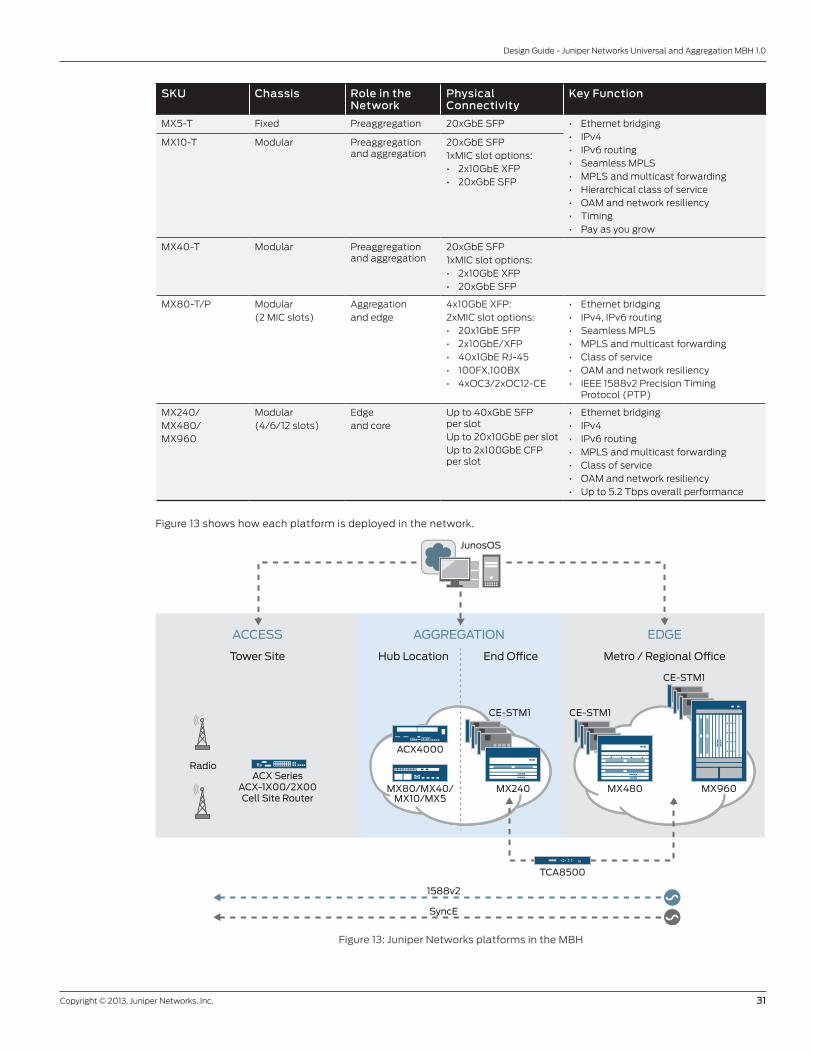
Copyright © 2013, Juniper Networks, Inc. 31
Design Guide - Juniper Networks Universal and Aggregation MBH 1.0
SKU Chassis Role in the Network
Physical Connectivity
Key Function
MX5-T Fixed Preaggregation 20xGbE SFP • Ethernet bridging• IPv4• IPv6 routing• Seamless MPLS• MPLS and multicast forwarding• Hierarchical class of service• OAM and network resiliency• Timing• Pay as you grow
MX10-T Modular Preaggregation and aggregation
20xGbE SFP1xMIC slot options:• 2x10GbE XFP• 20xGbE SFP
MX40-T Modular Preaggregation and aggregation
20xGbE SFP1xMIC slot options:• 2x10GbE XFP• 20xGbE SFP
MX80-T/P Modular (2 MIC slots)
Aggregationand edge
4x10GbE XFP:2xMIC slot options:• 20x1GbE SFP• 2x10GbE/XFP• 40x1GbE RJ-45• 100FX,100BX• 4xOC3/2xOC12-CE
• Ethernet bridging • IPv4, IPv6 routing• Seamless MPLS• MPLS and multicast forwarding• Class of service • OAM and network resiliency • IEEE 1588v2 Precision Timing
Protocol (PTP)
MX240/MX480/MX960
Modular (4/6/12 slots)
Edgeand core
Up to 40xGbE SFP per slotUp to 20x10GbE per slotUp to 2x100GbE CFP per slot
• Ethernet bridging • IPv4 • IPv6 routing • MPLS and multicast forwarding • Class of service• OAM and network resiliency• Up to 5.2 Tbps overall performance
Figure 13 shows how each platform is deployed in the network.
ACCESS AGGREGATION EDGE
ACX SeriesACX-1X00/2X00Cell Site Router
CE-STM1
CE-STM1
MX480
Tower Site Hub Location End O ce Metro / Regional O ce
MX960MX240
Radio
MX80/MX40/MX10/MX5
ACX4000
JunosOS
TCA8500
1588v2
SyncE
CE-STM1
Figure 13: Juniper Networks platforms in the MBH

32 Copyright © 2013, Juniper Networks, Inc.
Design Guide - Juniper Networks Universal and Aggregation MBH 1.0
The ACX1000, ACX2000, and ACX4000 routers are deployed at the cell site in the access network. ACX1000 and ACX
ACX2000 routers are designed according to the ETSI 300 standard and have a hardened fanless design that allows
installation in outdoor cabinets. For a more detailed platform description, see the “ACX Series Universal Access Routers”
product datasheet.
The ACX4000 and the smaller MX40 and MX80 routers are deployed in the preaggregation or aggregation segments.
For more detailed information about MX Series routers, see the “MX Series 3D Universal Edge Routers for the Midrange”
product datasheet.
Depending on the network scale, the high-end MX240 or MX480 platforms can be deployed at the large consolidated
central office (CO) in the aggregation segment of the MBH network. The larger capacity MX480 and MX 960 routers
are deployed in the point of presence (POP) at the edge of the core network segment. For more detailed information
about the high-end MX Series routers, see the “MX Series 3D Universal Edge Routers” product datasheet.
The TCA Timing Servers are primary reference sources, providing highly accurate timing that is critical for mobile
networks. These servers are a crucial part of the Juniper Networks solution for timing and synchronization. They use
GPS and a local oscillator to deliver Stratum 1 timing reference and exceptional holdover. They serve as grandmaster
clocks and are usually located at the CO or regional/metro POP with direct connectivity to collocated MX Series
routers. For more detailed information about TCA appliances, see the “TCA8000 and TCA8500 Timing Services”
product datasheet.
The Junos Space network management solution provides comprehensive fault, configuration, accounting, performance,
and security (FCAPS) end-to-end MBH network management and service provisioning. For more detailed information,
see the “Junos Space” product datasheet.

Copyright © 2013, Juniper Networks, Inc. 33
Design Guide - Juniper Networks Universal and Aggregation MBH 1.0
Part 2: Design and Planning This part includes the following topics:
• Design Considerations Workflow
• Topology Considerations
• MBH Service Profiles
• CoS Planning
• Timing and Synchronization Planning
• End-to-End IP/MPLS Transport Design
• MPLS Services Design for the 4G LTE Profile
• MPLS Service Design for the HSPA Service Profile
• MPLS Service Design for the 3G Service Profile
• MPLS Service Design for the 2G Service Profile
• OAM
• High Availability and Resiliency
• Network Management
• Design Consistency and Scalability Verification
Design Considerations WorkflowWhen you design an IP/MPLS access and aggregation network, the variety of available technologies and features is
very large, and this can result in extremely complicated designs. Complexity is an important consideration because very
often the MBH network is operated by service providers that are not experienced with IP and MPLS technologies and
that want to keep the complexity of the solution as close as possible to the operational complexity of legacy access
networks. This problem can be partly solved when you use automation and network management tools. In general, we
recommend that you keep your design simple and add new features only if you cannot solve a problem by changing the
topology or network architecture at the IP/MPLS transport or service levels.
Consider the following tasks as you approach the solution design:
• Gather service requirements.
• Check the physical topology.
• Check the traffic flow topology.
• Check the existing requirements of your particular network. (for example, you may have operators more familiar with
hub and spoke, which may influence your topology decisions).
• Decide on the design.
In this guide, we recommend the following workflow for designing the MBH network:
1. Define end-to-end service requirements.
2. Design the network topology and consider building blocks:
a. Network topology: segment and number of nodes in each segment
b. Type of the hardware and software platforms for each network segment
3. Define MBH network end-to-end services (or service profiles):
a. User-to-network interface (UNI) properties (TDM, ATM, Ethernet VLANs, IP addressing)
b. IP and MPLS service architecture
c. End-to-end CoS requirements
4. Design network-to-network (NNI) CoS profiles and rules.
5. Design the IP/MPLS transport.
6. Design IP and MPLS services.
7. Determine the timing and synchronization.

34 Copyright © 2013, Juniper Networks, Inc.
Design Guide - Juniper Networks Universal and Aggregation MBH 1.0
8. Design network high availability and resiliency:
a. Platform high availability
b. Transport layer resiliency
c. Service layer resiliency
9. Verify network and product scalability with respect to your network requirements and design decisions.
10. Reconsider your design if necessary.
11. Consider the network management system.
Gathering End-to-End Service RequirementsEnd-to-end service definition is the starting point. MBH networks provide transport services, which connect mobile
network elements. The design of your network is affected by the requirements and properties of the type of
connectivity. Table 6 lists the requirements, possible options to select, and area of the design most affected by the
various requirements.
Table 6: Requirements for MBH Network
Requirement Options Design Aspect Impacted by the Requirements
Datalink and network layer encapsulation
TDM , ATM, Ethernet, IP Platform capabilities, hardware configuration, and IP/MPLS service architecture
Type of end-to-end connectivity Point-to-point, point-to-multipoint, full mesh
IP/MPLS service architecture
Delay and jitter per traffic type CoS design at UNI and NNI levels
Bandwidth restrictions at UNI Restrict ingress and egress bandwidth Restrict per UNI or traffic type
Traffic policing and filtering at the UNI
Restoration time in case of link or node failure
IP/MPLS transport and service layer design
Timing and synchronization parameters
Frequency, phase Platform capabilities, network segmentation into regions, and physical topology
Overall bandwidth and number of endpoints connected to the network
2/10/100 Mbps per cell site Platform capabilities, network segmentation into regions, and physical topology
Designing the Network TopologyWhen you start to design your network topology, we recommend that you start by planning the network topology and
regions, then decide on the platforms you want to use in the various segments of the design.
Planning the Network Topology and Regions
The network topology (especially in the access segment) dramatically affects the complexity of the design at other
layers, so we strongly recommend that you plan carefully. Often, the topology itself is dictated by other factors, such
as the existing optical infrastructure, which can be difficult to change. You can plan the network segments (access,
preaggregation, and aggregation) and the number of devices in each interior gateway protocol (IGP) region, taking into
consideration restrictions on timing and synchronization, bandwidth requirements, and the overlaid transport layer.
Deciding on the Platforms to Use
Juniper Networks provides a broad portfolio of ACX Series and MX Series routers for the MBH solution, as shown in
Table 5. Note that the roles a router plays can be ambiguous. Positioning a router in a role depends on factors that are
uniquely defined within the context of a particular project only. For example:
• Control and data plane scalability, which depends on the topology and the number of nodes in each access and
preaggregation segment.
• Total platform throughput in terms of Gbps and packets per second (pps).
• Port type and density.
• Feature set—Juniper Networks is working on a consistent and unified feature set across all platforms. However, you need
to reconsider differences in hardware and software features on the various platforms.
• Environmental requirements, for example, use of outdoor cabinets for access and preaggregation nodes.
• Capital expenditure (CapEx) and operational expenditure (OpEx) considerations.
Copyright © 2013, Juniper Networks, Inc. 35
Design Guide - Juniper Networks Universal and Aggregation MBH 1.0
Defining the MBH Network Service ProfileMBH service profiles are defined by UNI properties, by IP/MPLS service architecture, and by CoS settings at the UNI.
Juniper Networks service definitions are aligned with MEF 22.1, MBH Phase 2 Implementation Agreement specification,
which contains detailed service definitions for MBH use cases.
Designing the MPLS Service Architecture
Each service profile includes one end-to-end MPLS service or a combination of MPLS services with a stitching point
somewhere in the middle of the MBH network. Part of the design consideration process is the decision you make about
the type of service and stitching point of the MPLS service. At this point, the design decision is driven by the initial
requirements, end-to-end requirements for the MBH network services, and considerations of network scalability.
To provide scalability, you must decide on the role of the service helper (for example, the Multiprotocol BGP (MP-BGP)
route reflector). When you use services like Layer 3 VPN with a full mesh topology between access nodes, think about
how to segment the network at the service level to restrict the number of VPN prefixes learned by each access router.
As soon as you make a decision about scaling and put the transport level in place, defining services is straightforward.
Consider network resiliency at the service layer after you make the decisions about scaling. Network resiliency is a
complex task, which is solved at different layers as discussed in High Availability and Resiliency.
Designing UNI Properties
User-to-network interface (UNI) definitions specify properties such as:
• Link layer encapsulation
• Service separation
• CoS at the UNI
Link Layer Encapsulation
The choice of the link layer technology (TDM, ATM, Ethernet, or IP) is dictated by the requirements of the RAN network
(2G, 3G, HSPA, 4G LTE) and defines the service profile of the MBH solution.
Service Separation
Service separation at the UNI level is automatically provided when you use SAToP or CESoPSN for TDM-based service
emulation at the physical or logical port level.
Assign ATM virtual path identifiers (VPIs) and virtual circuit identifiers (VCIs) at each UNI per ATM pseudowire service.
VPI and VCI pairs are assigned globally and are preserved across the entire MBH network.
When you use an Ethernet interface and the UNI, service separation is provided by means of VLANs. Each VLAN
represents a separate Layer 2 broadcast domain, which carries a separate service. In the context of the MBH network,
the VLAN numbering at the UNI level can be global or local. When the VLAN numbering is local, the VLAN number
is not preserved across the MBH network. Usually, not preserving the VLAN number gives the MBH service provider
additional flexibility in managing and planning services. ACX Series and MX Series routers support a choice of
technology for setting up a VLAN. The choices are the IEEE 802.1Q standard and the IEEE 802.1ad standard. Only the
IEEE 802.1Q standard is part of the Juniper Networks MBH solution.
In some LTE deployment scenarios, one logical interface (with the same VLAN and IP address) is used for all services.
In this case, the RAN and the EPC of the mobile network are responsible for service separation at the network or high
layers of the Open Systems Interconnection (OSI) model (Layer 4 – Layer 7).
Class of Service at the UNI
When planning and designing CoS rules, consider the following factors:
• The traffic profile and requirements of granular classification of traffic streams within a forwarding class (in our solution
we use a maximum of eight classes for each physical port with the proposed platform portfolio—ACX Series and MX
Series routers).
• A combination of multifield (MF) classifiers and behavior aggregate (BA) classifiers (only BA classifiers are used in
this guide).
• Type of class-of-service marking, which can be DSCP or 802.1p, depending on whether a service is Layer 2 or Layer 3, and
whether the incoming frames are VLAN tagged or not.

36 Copyright © 2013, Juniper Networks, Inc.
Design Guide - Juniper Networks Universal and Aggregation MBH 1.0
Designing NNI CoS Profiles and RulesAfter you define CoS profiles for the UNI, define consistent CoS rules across the entire MBH network for NNIs. Keep in
mind the following two points when you plan the CoS rules at the NNI:
• Use the MPLS code point (EXP bit) for traffic classification
• Add new traffic classes for network OAM protocols, network control protocols, and synchronization (IEEE 1588v2 PTP)
Designing the IP and MPLS Transport LayerDesigning the IP and MPLS transport layer is the most complex part of the design process. However, if you follow our
seamless MPLS architecture, you will be better prepared to make the correct decisions about mapping the network
topology to the architectural segments. (See the topic “Seamless MPLS.”) At the IP and MPLS transport level, you
determine which nodes perform the role of the area border router (ABR) or the autonomous system boundary router
(ASBR). After you designate the border routers, the roles of other nodes fall logically into place. Many protection
mechanisms are deployed at the IP and MPLS transport level and are included into the overall solution for MBH
network resiliency.
Designing Timing and SynchronizationThere are multiple ways to distribute timing information across the MBH network—traditional TDM-based timing
distribution, IEEE 1588v2, Synchronous Ethernet, and NTPv3 and v4. When applying CoS rules, you must highlight
packets carrying timing information into a high-priority, low-latency queue. Juniper Networks supports multiple
timing synchronization options because a single timing solution does not fit all network types or requirements.
IEEE 1588v2 is a versatile fit for the IP and Ethernet-based MBH because it is topology agnostic and supports both
frequency and phase.
Verifying the Network and Product ScalabilityThe design verification and consistency analysis are an important part of your design and planning process. This is
when you make a final check of the feature consistency across platforms and across software releases, which can
vary on different platforms. Also, you should ensure consistency of platform and network scalability and assess how
platform resources are used as the number of devices in the network increases. Also assess how network parameters
like timing and synchronization, resiliency, and time for network convergence after failure will evolve with the growing
network infrastructure. Sometimes, after such analysis, you have to reconsider some of your decisions. For example,
you might need to replace a preaggregation platform with more powerful devices or even change the IGP protocols or
the way nodes are combined into the IGP regions in the network.
Considering the Network Management SystemNetwork management is a separate process from all previous considerations. However, when we talk about deploying
a network, which could potentially consist of hundreds of thousands of routers, the role of network management and
automation plays an integral role in a carrier network. Proposed designs and feature sets at all levels and across all
platforms should be consistent with the network management system (NMS) and should make the NMS an integral
part of any MBH solution. NMS tasks are as follows:
• Element management
• Network management (IP and MPLS transport provisioning)
• Service provisioning
• Bulk service provisioning
• CoS provisioning
• OAM provisioning
• Network monitoring
• Service-level agreement (SLA) monitoring

Copyright © 2013, Juniper Networks, Inc. 37
Design Guide - Juniper Networks Universal and Aggregation MBH 1.0
Topology ConsiderationsPlanning the Network Segment and Regions Decisions about network topology dramatically influence the design of the transport layer and can add complexity or
allow you to create a straightforward transport infrastructure that can easily grow to practically any number of nodes.
When you plan the network segment and regions, your main task is to define the correct balance between complexity,
scalability, and failure resistance while you decide on the following parameters:
• How the mobile backhaul (MBH) network nodes fit into the MBH network segments:
- Access segment
- Preaggregation and aggregation segment
- Core segment
• The number of interior gateway protocol (IGP) regions
• The optimal number of devices in each IGP region
Access Segment
The implementation scenarios in this document address two special cases for the access segment that fit into the
above concepts and can be found in the deployment scenarios. These special cases in the access segment are:
• Ring topology
• Hub-and-spoke topology
Figure 14 illustrates ring-based access regions in the access segment where a pair of AG 1 routers and five CSRs build a
complete 1GbE ring and a 10GbE ring.
ServiceEdge
RemoteService
Edge
CORE NETWORKPRE-AGGREGATION
AGGREGATION
ACCESS
ACCESS
IP/MPLS
AG 1.1 AG 1.2
AG 1.3 AG 1.4
AG 3.1
AG 3.2
PE 1
PE 2AG 2.2
AG 2.1
SGW/PGW
PCRF
EPC
MMEHSS
Figure 14: Ring topology in an access segment

38 Copyright © 2013, Juniper Networks, Inc.
Design Guide - Juniper Networks Universal and Aggregation MBH 1.0
Figure 15 illustrates an alternative approach in which each cell site router (CSR) is dual homed to two AG 1 routers.
ServiceEdge
RemoteService
Edge
CORE NETWORKAGGREGATION
IP/MPLS
AG 3.1
AG 3.2
PE 1.1
PE 1.2AG 2.2
AG 2.1
PRE-AGGREGATION
ACCESS
ACCESS
AG 1.1 AG 1.2
AG 1.3 AG 1.4
SGW/PGW
PCRF
EPC
MMEHSS
Figure 15: Hub-and-spoke topology in the access segment
The design and implementation of the service plane are the same for both topologies—ring and hub and spoke—
because of the decoupling of the transport and service planes. Although some transport designs work better with
hub and spoke and some work better with access rings, this guide follows the principle of less complexity and
more versatility. Therefore, we recommend deployment scenarios that work well and are configured simply in both
topologies. However, this can mean fewer resiliencies in some failure scenarios or longer paths for ring topologies. Most
topology descriptions in this guide are shown for a ring topology with notes that describe the differences for a hub-
and-spoke topology.
Preaggregation and Aggregation Segments
In Figure 14 and Figure 15, each aggregation segment has two AG 2 routers that are peers to AG 3 routers with direct
10GbE links arranged in a full mesh. The implementation scenarios have two AG 2 routers in each aggregation segment.
The aggregation segment has an internal hierarchy and connects to the preaggregation segment. So AG 2 routers
connect a number of preaggregation AG 1 router rings together by means of 10GbE links. AG 1 routers, in turn, connect to
the access segment, which consists of multiple access regions. The number of AG 1 routers in an aggregation segment
depends on the number of access regions they interconnect and the geographic characteristics of the topology.
The total number of AG 1 and AG 2 routers in an aggregation domain should not exceed a reasonable figure, such as a
maximum of 200 to 300 routers. The term reasonable is used here in the context of traditional IP/MPLS networks that
generally use a single flat OSPF or IS-IS domain for the control plane to build the MPLS transport or data plane. The
network topology at the preaggregation and aggregation level can have any configuration that provides at least two
paths from any AG 1 router to an AG 2 router.
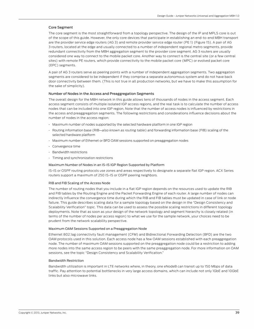
Copyright © 2013, Juniper Networks, Inc. 39
Design Guide - Juniper Networks Universal and Aggregation MBH 1.0
Core Segment
The core segment is the most straightforward from a topology perspective. The design of the IP and MPLS core is out
of the scope of this guide. However, the only core devices that participate in establishing an end-to-end MBH transport
are the provider service edge routers (AG 3) and remote provider service edge router (PE 1) (Figure 15). A pair of AG
3 routers, located at the edge and usually connected to a number of independent regional metro segments, provide
redundant connectivity from the MBH aggregation segment to the provider core segment. AG 3 routers are usually
considered one way to connect to the mobile packet core. Another way to connect is the central site (or a few central
sites) with remote PE routers, which provide connectivity to the mobile packet core (MPC) or evolved packet core
(EPC) segments.
A pair of AG 3 routers serve as peering points with a number of independent aggregation segments. Two aggregation
segments are considered to be independent if they comprise a separate autonomous system and do not have back
door connectivity between them. (This is not true in all production networks, but we have to make this assumption for
the sake of simplicity).
Number of Nodes in the Access and Preaggregation Segments
The overall design for the MBH network in this guide allows tens of thousands of nodes in the access segment. Each
access segment consists of multiple isolated IGP access regions, and the real task is to calculate the number of access
nodes that can be included into one IGP region. Note that the number of access nodes is influenced by restrictions in
the access and preaggregation segments. The following restrictions and considerations influence decisions about the
number of nodes in the access region:
• Maximum number of nodes supported by the selected hardware platform in one IGP region
• Routing information base (RIB—also known as routing table) and forwarding information base (FIB) scaling of the
selected hardware platform
• Maximum number of Ethernet or BFD OAM sessions supported on preaggregation nodes
• Convergence time
• Bandwidth restrictions
• Timing and synchronization restrictions
Maximum Number of Nodes in an IS-IS IGP Region Supported by Platform
IS-IS or OSPF routing protocols use zones and areas respectively to designate a separate flat IGP region. ACX Series
routers support a maximum of 250 IS-IS or OSPF peering neighbors.
RIB and FIB Scaling of the Access Node
The number of routing nodes that you include in a flat IGP region depends on the resources used to update the RIB
and FIB tables by the Routing Engine and the Packet Forwarding Engine of each router. A large number of nodes can
indirectly influence the convergence time during which the RIB and FIB tables must be updated in case of link or node
failure. This guide describes scaling data for a sample topology based on the design in the “Design Consistency and
Scalability Verification” topic. This data can be used to assess the possible scaling restrictions in different topology
deployments. Note that as soon as your design of the network topology and segment hierarchy is closely related (in
terms of the number of nodes per access region) to what we use for the sample network, your choices need to be
prudent from the network scalability perspective.
Maximum OAM Sessions Supported on a Preaggregation Node
Ethernet 802.1ag connectivity fault management (CFM) and Bidirectional Forwarding Detection (BFD) are the two
OAM protocols used in this solution. Each access node has a few OAM sessions established with each preaggregation
node. The number of maximum OAM sessions supported on the preaggregation node could be a restriction to adding
more nodes into the same access region to be peers with the same preaggregation node. For more information on OAM
sessions, see the topic “Design Consistency and Scalability Verification.”
Bandwidth Restriction
Bandwidth utilization is important in LTE networks where, in theory, one eNodeB can transit up to 150 Mbps of data
traffic. Pay attention to potential bottlenecks in very large access domains, which can include not only 1GbE and 10GbE
links but also microwave links.
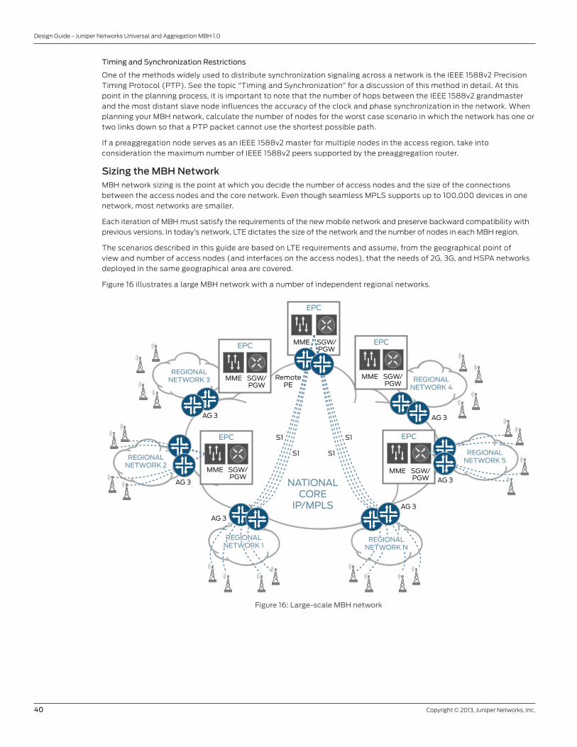
40 Copyright © 2013, Juniper Networks, Inc.
Design Guide - Juniper Networks Universal and Aggregation MBH 1.0
Timing and Synchronization Restrictions
One of the methods widely used to distribute synchronization signaling across a network is the IEEE 1588v2 Precision
Timing Protocol (PTP). See the topic “Timing and Synchronization” for a discussion of this method in detail. At this
point in the planning process, it is important to note that the number of hops between the IEEE 1588v2 grandmaster
and the most distant slave node influences the accuracy of the clock and phase synchronization in the network. When
planning your MBH network, calculate the number of nodes for the worst case scenario in which the network has one or
two links down so that a PTP packet cannot use the shortest possible path.
If a preaggregation node serves as an IEEE 1588v2 master for multiple nodes in the access region, take into
consideration the maximum number of IEEE 1588v2 peers supported by the preaggregation router.
Sizing the MBH NetworkMBH network sizing is the point at which you decide the number of access nodes and the size of the connections
between the access nodes and the core network. Even though seamless MPLS supports up to 100,000 devices in one
network, most networks are smaller.
Each iteration of MBH must satisfy the requirements of the new mobile network and preserve backward compatibility with
previous versions. In today’s network, LTE dictates the size of the network and the number of nodes in each MBH region.
The scenarios described in this guide are based on LTE requirements and assume, from the geographical point of
view and number of access nodes (and interfaces on the access nodes), that the needs of 2G, 3G, and HSPA networks
deployed in the same geographical area are covered.
Figure 16 illustrates a large MBH network with a number of independent regional networks.
NATIONALCORE
IP/MPLS
REGIONALNETWORK 3
REGIONALNETWORK 2
REGIONALNETWORK 5
REGIONALNETWORK 4
MME SGW/PGW
EPC
MME SGW/PGW
EPC
MME
EPC
MME SGW/PGW
EPC
MME SGW/PGW
EPC
AG 3
AG 3
RemotePE
AG 3
AG 3
AG 3
AG 3
S1 S1
S1 S1
REGIONALNETWORK 1
REGIONALNETWORK N
SGW/PGW
Figure 16: Large-scale MBH network

Copyright © 2013, Juniper Networks, Inc. 41
Design Guide - Juniper Networks Universal and Aggregation MBH 1.0
Each regional network connects to the national IP and MPLS core through an AG 3 edge router. Each regional network
with 10,000 access nodes might or might not have its own directly connected EPC. If an EPC is not installed in a
particular geographical region, then an EPC at the remote provider edge POP is used for that region.
The distribution and number of access nodes across a regional network segment—access, preaggregation, aggregation,
or core—is represented in Figure 17.
PRE-AGGREGATION
ACCESS
CORENETWORK
x4
AG 1x4
CSR x5
CSR x5
ACCESS
AG 3.1
AG 3.2AG 2.2
AG 2.1AG 1.1 AG 1.2
AG 1.3 AG 1.4
x16
x16
AGGREGATION
AG 2x2
CSR x5
MME
SGW/PGW
HSS
PCRF
EPC
Figure 17: Network segment sizing
In Figure 17, sixteen pairs of AG 2 aggregation routers interconnect with edge routers AG 3.1 and AG 3.2 by means of
direct 10GbE links. On the other side, each aggregation router pair—AG 2.1 with AG 2.2, AG 2.3 with AG 2.4, and so on—
interconnects sixteen preaggregation semirings. Each preaggregation semiring consists of four preaggregation (PRE-AG
G) routers (AG 1.1, AG 1.2, AG 1.3, AG 1.4, and so on) interconnected with 10GbE links. Finally, each pair of preaggregation
AG 1 routers interconnects four access rings with five CSRs in each access ring. CSRs within a ring are connected by
optical GbE links or by microwave lines with a total capacity of 400 Mbps for each ring.
Table 7 shows the number of nodes of each type in each segment and the number of access nodes aggregated at each
aggregation and preaggregation level.

42 Copyright © 2013, Juniper Networks, Inc.
Design Guide - Juniper Networks Universal and Aggregation MBH 1.0
Table 7: Sample Network Segment Size
Network Segment AG 3 Nodes AG 2 Nodes AG 1 Nodes AN Nodes Total
Regional network 2 32 1,024 10,240 11,298
AG 3 ring - 32 1,024 10,240 11,296
AG 2 ring - 2 64 640 706
AG 1 ring - - 4 40 44
The total number of nodes in one regional network is 11,298. If the national MBH network has 10 regional networks, the
total number of nodes equals approximately 100,000 nodes connected to the national IP and MPLS core.
After you define the infrastructure, node port density is derived automatically, providing the information that you need
to decide the platforms to use in each network segment.
The high-level topology is driven by LTE network requirements. If the same network needs to serve 2G, 3G, and
HSPA mobile networks, you must address additional considerations about the base station controller (BSC) and
radio network controller (RNC). These nodes usually coincide with the locations of the AG 2 nodes, so they must be
equipped with legacy interfaces to provide transport for TDM and ATM circuits if necessary.

Copyright © 2013, Juniper Networks, Inc. 43
Design Guide - Juniper Networks Universal and Aggregation MBH 1.0
MBH Service ProfilesWe defined four service profiles (one per mobile network type—2G, 3G, HSPA, and 4G LTE) as subsets of the overall
service architecture, which puts together a type of the user-to-network interface (UNI), a type of the MPLS service, and
an MPLS service topology with stitching points, and assigns service node functions to the MBH network nodes across
segments. Each profile can be planned, designed, and deployed independently.
This topic describes in more detail the four service profiles—2G, 3G, HSPA, and 4G LTE in relation to the MBH
service architecture.
4G LTE Service ProfileThe 4G LTE mobile network uses an IPv4 infrastructure to interconnect its entities. Providing IPv4 over Ethernet
connectivity is the main objective of the MBH network in this case. A variety of physical interface types, such as
100BASE/1000BASE-T/LX/SX, can be used to interconnect eNodeB to the MBH CSR.
The following three types of interfaces are defined within the 4G LTE mobile infrastructure:
• S1-U—An over-IP interface that carries user data traffic from eNodeB to the Serving Gateway (SGW). SGW is an element
of the EPC.
• S1-MME—An over-IP interface between eNodeB and the mobility management entity (MME) that carries control plane
traffic used to manage and control mobile entities. MME is an element of the EPC.
• X2—An over-IP interface between two eNodeBs that is used to manage and control mobile entities at the time of
handover between eNodeBs.
To provide connectivity between mobile network elements over an MBH network for these interfaces, you can use
MPLS Layer 2 or Layer 3 services. Building a large-scale, full meshed MPLS Layer 2 network is a very complex task, and
we recommend avoiding it if possible. Instead, we recommend that you use MPLS Layer 3 services.
Figure 18 illustrates the recommended service architecture for a 4G LTE service profile. A separate logical Layer 2 and
Layer 3 interface between the eNodeB and the access node is used per mobile network interface (S1-MME, S1-U, X2).
Each eNodeB connects the access node over a physical GbE port. At Layer 2, VLAN tagging is implemented at the UNI
to separate traffic between logical interfaces. At Layer 3, you assign an IP address to each logical interface and place
it into a separate Layer 3 MPLS VPN, which provides end-to-end connectivity between eNodeBs and EPC elements
across the MBH network and for each mobile network interface—S1-MME, S1-U, and X2. In Figure 18, these Layer 3 VPNs
are S1-MME, S1-U, and X2 services mapped to the mobile network interfaces S1-MME, S1-U, and X2, respectively. If
your eNodeB supports one IP interface, you can use one VLAN and one logical interface in one VRF, instead of three IP
addresses, three VLANs, and three VRFs, as in our example.
MME
SGW/PGW
EPC
VLAN S1-MME
VLAN X2 S1-MME
S1-uPE
eNode B
eNode B VLAN S1-u
VLAN S1-MME
VLAN X2
VLAN S1-u
LogicalInterface
Physical Port
1588v2 on Separate VLAN in GRT
1588v2Grandmaster
X2
SN SN
IP/MPLSMBH
AN
AN
L3 VPN for S1-MME
L3 VPN for X2
L3 VPN for S1-u
Timing
S1-MME
S1-u
1588v2
Figure 18: Recommended service architecture for 4G LTE service profile
The dotted lines in Figure 18 show connectivity within the Layer 3 VPNs.

44 Copyright © 2013, Juniper Networks, Inc.
Design Guide - Juniper Networks Universal and Aggregation MBH 1.0
Depending on the type of uplink and downlink separation technology used for the air interface, requirements are
different. A 4G LTE network with time-division duplex (TDD) LTE at the air interface requires both frequency and phase
synchronization. MBH can deliver both.
Synchronous Ethernet is most commonly used to provide frequency synchronization and is a very reliable method
because the synchronization signal is distributed at the physical layer. All platforms in the MBH network that stay on
the path of signal distribution should support this feature. However, Synchronous Ethernet does not address the needs
of the mobile network that requires phase synchronization. The IEEE 1588v2 Precision Timing Protocol (PTP) is used
to address this requirement. Both methods (Synchronous Ethernet and IEEE 1588v2) complement each other, and can
be deployed simultaneously. The timing and synchronization distribution are shown in Figure 18 and Figure 19. The blue
dotted lines in Figure 18 represent IEEE 1588v2, and the blue dotted lines in Figure 19 represent Synchronous Ethernet.
Defining the CoS Attribute at the UNI Interface
Class-of-service (CoS) attributes are an essential part of the MBH 4G LTE service profile definition. Traffic
classification with regard to CoS can be defined as follows:
• Behavior aggregate classifiers—IEEE 802.1p or Differentiated Services code point (DSCP) classifiers at the ingress UNI
• Logical interface classifiers—Mapped to a particular VLAN
• Multifield classifier—Based on the IP source prefixes of the S1-U, S1-MME, and X2 interfaces
All the deployment scenarios in this guide use a CoS configuration in which all traffic is marked with the correct CoS
attribute by eNodeB or EPC before it arrives at the MBH UNI. After that, the BA mechanism is used to map traffic to the
forwarding class for CoS management throughout the network.
HSPA Service ProfileThe HSPA service profile is defined for the HSPA universal mobile telecommunications system (UMTS) mobile
network, which is capable of using the Iub interface over an IP or Ethernet interface. This type of Iub interface is
used to carry user data from an HSPA NodeB to an HSPA RNC over Layer 3 services. NodeB or RNC is responsible
for Iub encapsulation into the IP interface with the MBH network access node by using IPv4 over Ethernet. You can
use different types of Ethernet ports to interconnect NodeB to the MBH network—100BASE-T/LX/SX interfaces or
1000BASE-T/LX/SX interfaces.
There are three different deployment scenarios from the MPLS service architecture perspective:
• End-to-end Layer 3 VPN
• Layer 2 VPN to Layer 3 VPN termination
• Layer 2 VPN to VPLS termination (Hierarchical VPLS)
End-to-End Layer 3 VPN
The design for end-to-end Layer 3 VPN is identical to the design described for the 4G LTE service profile in 4G LTE
Service Profile.
Layer 2 VPN to Layer 3 VPN Termination
This deployment scenario uses Layer 3 VPN, which transports Iub interface traffic defined in the Third-Generation
Partnership Project (3GPP) standards for Iub over IP infrastructure. The actual service node function can be located
either on the CSR or somewhere in the preaggregation segment. (See Figure 19.)
RNC
3G PCIub IP
Iub IPNode B
Node B
IP/MPLSAGGREGATION
IP/MPLSACCESS
Sync Ethernet
AN
AN
PEAG 1
Serves as SN
L2 Pseudowireto L3 VPN
Iub IP
L2 Pseudowire
Timing
VPLS
Figure 19: HSPA service profile with end-to-end layer 3VPN and pseudowire in the access segment

Copyright © 2013, Juniper Networks, Inc. 45
Design Guide - Juniper Networks Universal and Aggregation MBH 1.0
To extend service delivery from the service node, use a Layer 2 circuit (Layer 2 VPN) between the service node and
the CSR or access node. Usually the point of service delivery is placed somewhere at the border between segments
and can be a preaggregation or aggregation router. The Layer 2 pseudowire is terminated directly into the Layer 3 VPN
where a special stitching technique is used. The exact placement of the Layer 3 service delivery point within the MBH
network and the stitching technique become clearer after we discuss the network topology in the “MPLS Service Design
for the HSPA Service Profile” topic.
Usually, 3G mobile networks require frequency synchronization only. In this example, we use Synchronous Ethernet to
provide necessary functionality—the blue dotted line in Figure 19. Note that the timing and synchronization in the MBH
network are independent of the service profile, so a combination of different techniques can be used.
Class-of-service traffic marking is fulfilled on the basis of 802.1p at the cell site router in the CoS model.
End-to-End Hierarchical VPLS
Hierarchical VPLS in the access and aggregation network represents another valuable scenario for HSPA networks that
use Iub over Ethernet. The service architecture is very similar to the architecture in the 4G LTE and HSPA examples.
A router in the preaggregation or aggregation segments serves as the service node (SN)—AG 1 with the VPLS hub in
Figure 20—with multiple CSRs as VPLS spokes in the access segment extending service delivery to the physical and
logical UNI with Layer 2 pseudowires. Each service is represented by a single physical or logical interface at the access
router.
RNC
3G PCIub IP
Iub IPNode B
Node B
IP/MPLSAGGREGATION
IP/MPLSACCESS
Sync Ethernet
AN
AN
PEAG 1
L2 Pseudowireto VPLS
Iub IP
L2 Pseudowire
Timing
VPLS
Serves as SN
Figure 20: HSPA service profile with end-to-end VPLS
Class-of-service, timing, and synchronization requirements are the same as in the HSPA service profile scenario.
3G and 2G Service Profiles The 3G and 2G series of scenarios for transporting Iub and Abis traffic for HSPA and 2G networks use legacy ATM and
TDM interfaces. MBH services are represented at both ends of the network by the physical interface and encapsulation
type—on one side by NodeB and on BTS, on the other side by RNC and BSC. All traffic on the physical interface is
encapsulated into an MPLS pseudowire (SAToP, CESoPSN, or ATM pseudowire [PW3]), mapped to a unique forwarding
class (usually strict-high), and transported though the MBH network. (See Figure 21.)
3G PC
IubATM/TDM
AN
AN
AGAbis/TDM
Iub ATM/TDM
Abis TDM
BTS
Node B
IP/MPLSAGGREGATION
IP/MPLSACCESS
Sync Ethernet
Sync over E1/T1
Sync over E1/T1
SAToP/CESoP/ATM Pseudowire2G BSC
L2 Pseudowire
Timing
Figure 21: 3G and 2G networks with ATM and TDM interfaces

46 Copyright © 2013, Juniper Networks, Inc.
Design Guide - Juniper Networks Universal and Aggregation MBH 1.0
To place the circuit emulation traffic into the appropriate forwarding class within the access node configuration, CoS
rules are defined as a part of the MPLS service itself. (See the topic “CoS Planning” for more details.)
Unlike legacy networks that commonly use in-band synchronization mechanisms within the same TDM circuit, in this
scenario (as in the previous scenarios), you implement an out-of-band technique to distribute synchronization across
the network and reset the circuit at the UNI level. We position Synchronous Ethernet as the primary method for delivering
timing and synchronization to CSRs from the source connected at the aggregation network, as shown in Figure 21.
Clocking for the NodeB or BTS is further provided from the CSR over the same E1 and T1 or dedicated interface.
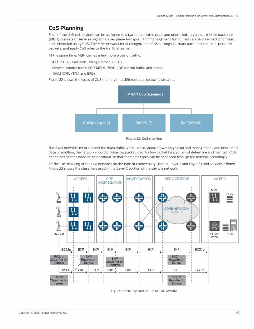
Copyright © 2013, Juniper Networks, Inc. 47
Design Guide - Juniper Networks Universal and Aggregation MBH 1.0
CoS PlanningEach of the defined services can be assigned to a particular traffic class and prioritized. In general, mobile backhaul
(MBH) consists of services signaling, user plane transport, and management traffic that can be classified, prioritized,
and scheduled using CoS. The MBH network must recognize the CoS settings, re-mark packets if required, prioritize
packets, and apply CoS rules to the traffic streams.
At the same time, MBH carries a few more types of traffic:
• IEEE 1588v2 Precision Timing Protocol (PTP)
• Network control traffic (IGP, MPLS, RSVP, LDP control traffic, and so on)
• OAM (CFP, Y1731, and BFD)
Figure 22 shows the types of CoS marking that differentiate the traffic streams.
802.1p (Layer 2) EXP (MPLS)DSCP (IP)
IP RAN CoS Scenarios
Figure 22: CoS marking
Backhaul networks must support the main traffic types—voice, video, network signaling and management, and best-effort
data. In addition, the network should provide low packet loss. For low packet loss, you must determine and maintain CoS
definitions at each node in the backhaul, so that the traffic types can be prioritized through the network accordingly.
Traffic CoS marking at the UNI depends on the type of connectivity (that is, Layer 2 and Layer 3) and services offered.
Figure 23 shows the classifiers used in the Layer 2 portion of the sample network.
DSCP
802.1p802.1p
DSCP
EXP EXP EXP EXP EXP EXP
EXP EXP EXP EXP EXP EXP
ACCESS SERVICE EDGEPRE-AGGREGATION
AGGREGATION 4G EPC
CORE NETWORKIP/MPLS
MME
SGW/PGW
HSS
PCRF
DSCPClassifier on
Ingress
DSCPRewrite on
Egress
802.1pClassifier on
Ingress
802.1pRewrite on
Egress
EXPRewrite on
EgressEXP
Classifier onIngress
eNode B
Figure 23: 802.1p and DSCP to EXP rewrite

48 Copyright © 2013, Juniper Networks, Inc.
Design Guide - Juniper Networks Universal and Aggregation MBH 1.0
In Figure 23, we use 802.1p and DSCP classifiers when applying CoS to tagged or untagged frames. The cell site devices
perform queuing, scheduling, and prioritization based on the 802.1p, DSCP, or both 802.1p and DSCP bit marking.
When the frames need to be transported across the backhaul network using MPLS label-switched paths (LSPs), EXP
classifiers are used within the core to classify packets, and the 802.1p or DSCP CoS values need to be rewritten into
EXP markings at the access node and transported over the LSPs.
Typically, behavior aggregate (BA) classifiers are used together with schedulers to achieve the required CoS guarantees
in a network. However, using a combination of BA and multifield (MF) classifiers introduces an extra level of granularity.
You can prioritize traffic streams within a particular class on the basis of VLAN IP source addressing.
When you configure CoS classification and rewrite rules, you assign each packet to a particular forwarding class. In the
deployment scenarios in this guide, each network node provides eight forwarding classes at each physical UNI and NNI
port. Each forwarding class is mapped to one of eight queues, and each queue can be assigned a priority. Priority, in its
turn, defines how traffic in the queue is scheduled. Higher priority queues are serviced before lower priority queues in
a weighted round-robin fashion. MX Series and ACX Series routers have some differences in the way they assign and
serve queue priorities.
MX Series routers use the following definitions:
• Strict high—The highest possible priority level. Traffic in this queue does not have any bandwidth limitations and is
restricted only by physical port bandwidth. This traffic is always serviced before any other queue receives bandwidth.
While there is traffic in the queue, strict-high traffic is serviced first along with the in-contract high priority queues. Only
one strict-high priority queue can be assigned at one time.
• High—This queue has the same priority level as strict-high. However, traffic in this queue is restricted by the committed
information rate (CIR). While traffic load is below the configured CIR bandwidth, it is served first or in a weighted round-
robin fashion with strict-high and other high priority queues.
• Medium high—The traffic in this queue is serviced when it is below its CIR and there is not any traffic in the queues with
higher priorities. If there are multiple medium-high priority queues, they are served in a weighted round-robin fashion.
• Medium low—The traffic in this queue is serviced when it is below its CIR and there is not any traffic in the queues with
higher priorities. If there are multiple medium-high priority queues, they are served in a weighted round-robin fashion.
• Low—The traffic in this queue is served when it is below its CIR and there is not any traffic in the queues with higher
priorities. If there are multiple medium-high priority queues, they are served in a weighted round-robin fashion.
ACX Series routers use the following definitions:
• Strict high—The highest possible priority level. Traffic in this queue does not have any bandwidth limitations and is
restricted only by physical port bandwidth. This traffic is always serviced before any other queue. While there is traffic in
the queue, strict-high traffic is serviced first. Multiple queues can be configured with strict-high priority at the same time.
• High—Although high, medium-high, medium-low, and low priority levels are not supported on ACX Series routers,
this behavior can be achieved by assigning a strict-high priority with a shaping rate. In this guide, we refer to such a
configuration on ACX Series routers as a high priority.
• Weighted deficit round-robin scheduling queue—The traffic in this queue is serviced when it is below its CIR and there is
not any traffic in the queues with higher priorities. Although high, medium-high, medium-low, and low priority levels are
not supported on ACX Series routers, in this guide, we refer to this priority level as a low priority.
Mobile technology standards define classes that can be used for traffic classification but do not mandate the number
of these classes that are actually used. This number depends on the network implementation and traffic profile. In
general, differentiation between the traffic types is done when you mark and prioritize packets as high, medium, or low.
The prioritization depends on the traffic type.
Four classes of traffic—background, interactive, streaming, and conversational—are defined for 3GPP-based
technologies such as UMTS. A system of nine QoS class identifiers (QCIs) are defined for 4G LTE.
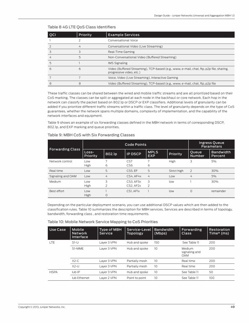
Copyright © 2013, Juniper Networks, Inc. 49
Design Guide - Juniper Networks Universal and Aggregation MBH 1.0
Table 8 4G LTE QoS Class Identifiers
QCI Priority Example Services
1 2 Conversational Voice
2 4 Conversational Video (Live Streaming)
3 3 Real-Time Gaming
4 5 Non-Conversational Video (Buffered Streaming)
5 1 IMS Signaling
6 6 Video (Buffered Streaming), TCP-based (e.g., www, e-mail, chat, ftp, p2p file, sharing, progressive video, etc.)
7 7 Voice, Video (Live Streaming), Interactive Gaming
8 8 Video (Buffered Streaming), TCP-based (e.g., www, e-mail, chat, ftp, p2p file
These traffic classes can be shared between the wired and mobile traffic streams and are all prioritized based on their
CoS marking. The classes can be spilt or aggregated at each node in the backhaul or core network. Each hop in the
network can classify the packet based on 802.1p or DSCP or EXP classifiers. Additional levels of granularity can be
added if you prioritize different traffic streams within a traffic class. The level of granularity depends on the type of CoS
guarantees, whether the network spans multiple domains, complexity of implementation, and the capability of the
network interfaces and equipment.
Table 9 shows an example of six forwarding classes defined in the MBH network in terms of corresponding DSCP,
802.1p, and EXP marking and queue priorities.
Table 9: MBH CoS with Six Forwarding Classes
Forwarding Class Code Points Ingress Queue
Parameters
Loss- Priority 802.1p IP DSCP MPLS
EXP Priority Queue Number
Bandwidth Percent
Network control LowHigh
76
CS7CS6
76
High 3 5%
Real time Low 5 CS5, EF 5 Strict high 2 30%
Signaling and OAM Low 4 CS4, AF4x 4 Low 4 5%
Medium LowHigh
32
CS3, AF3xCS2, AF2x
32
low 1 30%
Best effort LowHigh
10
CS1, AF1x 1 low 0 remainder
Depending on the particular deployment scenario, you can use additional DSCP values which are then added to the
classification rules. Table 10 summarizes the description for MBH services. Services are described in terms of topology,
bandwidth, forwarding class , and restoration time requirements.
Table 10: Mobile Network Service Mapping to CoS Priorities
Use Case Mobile Network Interface
Type of MBH Service
Service-Level Topology
Bandwidth (Mbps)
Forwarding Class
Restoration Time* (ms)
LTE S1-U Layer 3 VPN Hub and spoke 150 See Table 11 200
S1-MME Layer 3 VPN Hub and spoke 10 Medium signaling and OAM
200
X2-C Layer 3 VPN Partially mesh 10 Real time 200
X2-U Layer 3 VPN Partially mesh 10 Real time 200
HSPA Iub IP Layer 3 VPN Hub and spoke 10 See Table 11 50
Iub Ethernet Layer 2 VPN Point to point 10 See Table 11 100

50 Copyright © 2013, Juniper Networks, Inc.
Design Guide - Juniper Networks Universal and Aggregation MBH 1.0
Use Case Mobile Network Interface
Type of MBH Service
Service-Level Topology
Bandwidth (Mbps)
Forwarding Class
Restoration Time* (ms)
3G Iub ATM ATM pseudowire Point to point 10 Real time 100
2G Abis TDM CESoPSN Point to point 10 Real time <50
Abis TDM SAToP Point to point 10 Real time 50
* Restoration time requirement values represent sample values and are not guaranteed by the solutions described in
this guide, because they can significantly vary depending on the deployment in the field.
Table 11 lists the recommended mapping used in this guide between 3GPP CoS classes and the MBH network
forwarding classes. It also provides the classification preferences for mobile OAM traffic, MBH network control traffic,
and packet synchronization.
Table 11: Mobile Network Services Mapping to MBH CoS
Type of Traffic Forwarding Class Loss Priority
HSPA Background Best effort Low
Conversational Real time Low
Streaming Medium Low
Interactive Medium High
4G LTE QCI 1 Real time Low
QCI 2,QCI 3, QCI 4 Medium Low
QCI 5 Signaling and OAM Low
QCI 6, QCI 7, QCI 8 Medium High
QCI 9 Best effort Low
Mobile OAM Signaling and OAM Low
Time and synchronization IEEE 1588v2 Network control Low
Network control traffic IGP, BGP, OSPF, ISIS CFM, BFD, and so on
Network control Low
For CoS planning, keep the following general principles in mind:
• Any type of voice or conversational, real-time traffic (packet or circuit) is serviced by a forwarding class with a strict-high
priority queue.
• Any user data traffic, depending on the type of traffic (real-time gaming, streaming, Internet) and the application
requirements, is serviced within the medium forwarding class that has a loss priority higher than the mobility
signaling traffic.
• Any mobility signaling traffic is serviced within the medium forwarding class with a low loss priority.
• If it is possible to differentiate between S1 and X2 traffic flows—for example, different logical interfaces used at the
UNI for traffic belonging to X2 and S2—then the X2 traffic flow is serviced as real-time traffic.
• Any circuit-emulated traffic is serviced as real-time traffic with a strict-high priority queue.
Network control protocols, MBH OAM protocols, and synchronization (IEEE 1588v2) are crucial for transport-level
stability, fast failure detection, network convergence, and mobile network stability. All traffic types that are sensitive
to delay and jitter and share the same high priority queue affect each other. Pay attention to the way you design these
forwarding classes in different MBH segments. For example, the amount of BFD traffic can be significantly different in
access and aggregation segments, whereas synchronization can be represented by approximately the same amount of
traffic across MBH segments. Ideally, the IEEE 1588v2 traffic should be placed into a separate queue.
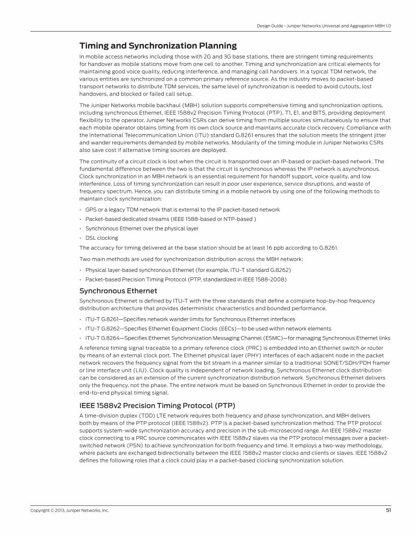
Copyright © 2013, Juniper Networks, Inc. 51
Design Guide - Juniper Networks Universal and Aggregation MBH 1.0
Timing and Synchronization PlanningIn mobile access networks including those with 2G and 3G base stations, there are stringent timing requirements
for handover as mobile stations move from one cell to another. Timing and synchronization are critical elements for
maintaining good voice quality, reducing interference, and managing call handovers. In a typical TDM network, the
various entities are synchronized on a common primary reference source. As the industry moves to packet-based
transport networks to distribute TDM services, the same level of synchronization is needed to avoid cutouts, lost
handovers, and blocked or failed call setup.
The Juniper Networks mobile backhaul (MBH) solution supports comprehensive timing and synchronization options,
including synchronous Ethernet, IEEE 1588v2 Precision Timing Protocol (PTP), T1, E1, and BITS, providing deployment
flexibility to the operator. Juniper Networks CSRs can derive timing from multiple sources simultaneously to ensure that
each mobile operator obtains timing from its own clock source and maintains accurate clock recovery. Compliance with
the International Telecommunication Union (ITU) standard G.8261 ensures that the solution meets the stringent jitter
and wander requirements demanded by mobile networks. Modularity of the timing module in Juniper Networks CSRs
also save cost if alternative timing sources are deployed.
The continuity of a circuit clock is lost when the circuit is transported over an IP-based or packet-based network. The
fundamental difference between the two is that the circuit is synchronous whereas the IP network is asynchronous.
Clock synchronization in an MBH network is an essential requirement for handoff support, voice quality, and low
interference. Loss of timing synchronization can result in poor user experience, service disruptions, and waste of
frequency spectrum. Hence, you can distribute timing in a mobile network by using one of the following methods to
maintain clock synchronization:
• GPS or a legacy TDM network that is external to the IP packet-based network
• Packet-based dedicated streams (IEEE 1588-based or NTP-based )
• Synchronous Ethernet over the physical layer
• DSL clocking
The accuracy for timing delivered at the base station should be at least 16 ppb according to G.8261.
Two main methods are used for synchronization distribution across the MBH network:
• Physical layer-based synchronous Ethernet (for example, ITU-T standard G.8262)
• Packet-based Precision Timing Protocol (PTP, standardized in IEEE 1588-2008)
Synchronous Ethernet Synchronous Ethernet is defined by ITU-T with the three standards that define a complete hop-by-hop frequency
distribution architecture that provides deterministic characteristics and bounded performance.
• ITU-T G.8261—Specifies network wander limits for Synchronous Ethernet interfaces
• ITU-T G.8262—Specifies Ethernet Equipment Clocks (EECs)—to be used within network elements
• ITU-T G.8264—Specifies Ethernet Synchronization Messaging Channel (ESMC)—for managing Synchronous Ethernet links
A reference timing signal traceable to a primary reference clock (PRC) is embedded into an Ethernet switch or router
by means of an external clock port. The Ethernet physical layer (PHY) interfaces of each adjacent node in the packet
network recovers the frequency signal from the bit stream in a manner similar to a traditional SONET/SDH/PDH framer
or line interface unit (LIU). Clock quality is independent of network loading. Synchronous Ethernet clock distribution
can be considered as an extension of the current synchronization distribution network. Synchronous Ethernet delivers
only the frequency, not the phase. The entire network must be based on Synchronous Ethernet in order to provide the
end-to-end physical timing signal.
IEEE 1588v2 Precision Timing Protocol (PTP)A time-division duplex (TDD) LTE network requires both frequency and phase synchronization, and MBH delivers
both by means of the PTP protocol (IEEE 1588v2). PTP is a packet-based synchronization method. The PTP protocol
supports system-wide synchronization accuracy and precision in the sub-microsecond range. An IEEE 1588v2 master
clock connecting to a PRC source communicates with IEEE 1588v2 slaves via the PTP protocol messages over a packet-
switched network (PSN) to achieve synchronization for both frequency and time. It employs a two-way methodology,
where packets are exchanged bidirectionally between the IEEE 1588v2 master clocks and clients or slaves. IEEE 1588v2
defines the following roles that a clock could play in a packet-based clocking synchronization solution.

52 Copyright © 2013, Juniper Networks, Inc.
Design Guide - Juniper Networks Universal and Aggregation MBH 1.0
Ordinary Clock Master
Master clock operation is the role that sends the clients (slave and boundary) the necessary messages that allow the
clients to establish their relative time distance and offset from this master’s clock or clock reference. The IEEE 1588v2
master clocks might have various sources for frequency and time information. Typically, Global Navigation Satellite
Systems (GNSS) is used. The delivery mechanism to the clients is either unicast or multicast packets over Ethernet
or UDP. If multiple master clocks are available in a network segment, a grandmaster is elected by means of Announce
messages, and all the other clocks synchronize directly with the grandmaster.
Ordinary Clock Slave
A slave clock or PTP client performs frequency and phase recovery based on received and requested timestamps
from the (grand) master. The recovery algorithm is one of the key differentiating factors between implementations
of vendors and their performance. A slave implementation recovers frequency and phase or time of day, and presents
both to the chassis and system on which it is running. The recovered clock can be distributed further with a variety of
methods such as BITS, Synchronous Ethernet, SONET/SDH, and even IEEE 1588v2. The latter case is an example of a
boundary clock, in which the slave and master clock functionality is found in one and the same node.
Boundary Clock
A boundary clock acts as an IEEE 1588v2 slave on one port and master on other ports. It synchronizes itself to a
grandmaster clock through a slave port, and supports synchronization of slaves to it on master ports. Boundary clocks
can improve the accuracy of the synchronization by reducing the number of IEEE 1588v2-unaware hops between the
grandmaster and the slave. You can deploy boundary clocks to deliver better scale because they reduce the number of
sessions and the number of packets per second on the master clock.
Transparent Clock
A transparent clock provides functionality to record the residence time in a single network node (that is, the time it took
for this node to forward this packet) for the PTP packets. The slave can remove the packet delay variation caused by a
node en route, delivering a higher precision clock. An added advantage of the transparent clock is that it does not have
to maintain any sessions for the PTP packets. It does, however, require all the routers en route to support the capability
of modifying the timing packets while forwarding them.
The first three methods are currently supported on the following Juniper Networks platforms—ACX Series, MX Series,
and the TCA Series.
Synchronization DesignOur comprehensive support for clocking on the ACX Series and MX Series platforms, combined with leading Junos OS
capabilities, enables several use cases. The goal is to deliver frequency, time, phase, time of day, or all these features,
from the network core to the customer edge (CE). The following three use cases are described in this guide:
• End-to-end IEEE 1588v2 with a boundary clock
• End-to-End IEEE 1588v2 in combination with other methods such as GNSS (10 MHz), BITS-T1 or E1, PPS and
Synchronous Ethernet
• Synchronous Ethernet in combination with other methods, such as GNSS (10 MHz), BITS-T1 or E1, PTP
End-to-End IEEE 1588v2 with a Boundary Clock
Figure 24 illustrates an IEEE 1588v2 scenario in which PTP provides synchronization from the grandmaster (GM), on the
right, to the NodeB on the left through a direct PTP session or through a chain of boundary clocks.
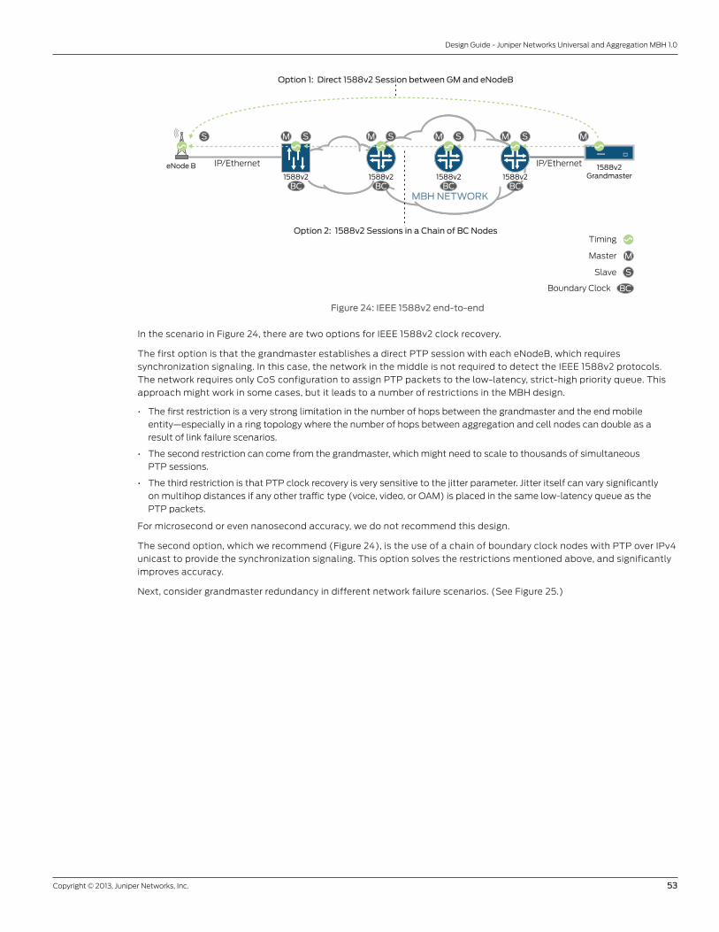
Copyright © 2013, Juniper Networks, Inc. 53
Design Guide - Juniper Networks Universal and Aggregation MBH 1.0
eNode B
1588v21588v2
Grandmaster
Option 1: Direct 1588v2 Session between GM and eNodeB
Option 2: 1588v2 Sessions in a Chain of BC Nodes
IP/EthernetIP/Ethernet
MBH NETWORK
1588v2 1588v21588v2
S M S M S M S M S
Timing
Master M
Slave S
M
BC BC BC BC
BCBoundary Clock
Figure 24: IEEE 1588v2 end-to-end
In the scenario in Figure 24, there are two options for IEEE 1588v2 clock recovery.
The first option is that the grandmaster establishes a direct PTP session with each eNodeB, which requires
synchronization signaling. In this case, the network in the middle is not required to detect the IEEE 1588v2 protocols.
The network requires only CoS configuration to assign PTP packets to the low-latency, strict-high priority queue. This
approach might work in some cases, but it leads to a number of restrictions in the MBH design.
• The first restriction is a very strong limitation in the number of hops between the grandmaster and the end mobile
entity—especially in a ring topology where the number of hops between aggregation and cell nodes can double as a
result of link failure scenarios.
• The second restriction can come from the grandmaster, which might need to scale to thousands of simultaneous
PTP sessions.
• The third restriction is that PTP clock recovery is very sensitive to the jitter parameter. Jitter itself can vary significantly
on multihop distances if any other traffic type (voice, video, or OAM) is placed in the same low-latency queue as the
PTP packets.
For microsecond or even nanosecond accuracy, we do not recommend this design.
The second option, which we recommend (Figure 24), is the use of a chain of boundary clock nodes with PTP over IPv4
unicast to provide the synchronization signaling. This option solves the restrictions mentioned above, and significantly
improves accuracy.
Next, consider grandmaster redundancy in different network failure scenarios. (See Figure 25.)
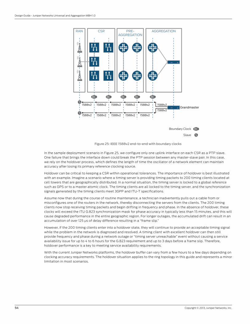
54 Copyright © 2013, Juniper Networks, Inc.
Design Guide - Juniper Networks Universal and Aggregation MBH 1.0
Grandmaster1588v2 1588v2 1588v2 1588v2 1588v2
1588v2 1588v2 1588v2 1588v2 1588v2
1588v2
1588v2
RAN CSR PRE-AGGREGATION
AGGREGATION
S
BC BC BC BC BC
S
BCBoundary Clock
Slave S
Figure 25: IEEE 1588v2 end-to-end with boundary clocks
In the sample deployment scenario in Figure 25, we configure only one uplink interface on each CSR as a PTP slave.
One failure that brings the interface down could break the PTP session between any master-slave pair. In this case,
we rely on the holdover process, which defines the length of time the oscillator of a network element can maintain
accuracy after losing its primary reference clocking source.
Holdover can be critical to keeping a CSR within operational tolerances. The importance of holdover is best illustrated
with an example. Imagine a scenario where a timing server is providing timing packets to 200 timing clients located at
cell towers that are geographically distributed. In a normal situation, the timing server is locked to a global reference
such as GPS or to a master atomic clock. The timing clients are all locked to the timing server, and the synchronization
signals generated by the timing clients meet 3GPP and ITU-T specifications.
Assume now that during the course of routine maintenance, a technician inadvertently pulls out a cable from or
misconfigures one of the routers in the network, thereby disconnecting the servers from the clients. The 200 timing
clients now stop receiving timing packets and begin drifting in frequency and phase. In the absence of holdover, these
clocks will exceed the ITU G.823 synchronization mask for phase accuracy in typically less than 15 minutes, and this will
cause degraded performance in the entire geographic region. For longer outages, the accumulated drift can result in an
accumulation of over 125 µs of delay difference resulting in a “frame slip.”
However, if the 200 timing clients enter into a holdover state, they will continue to provide an acceptable timing signal
while the problem in the network is diagnosed and resolved. A timing client with excellent holdover can then still
provide frequency and phase during a network outage or “timing server unreachable” event without causing a service
availability issue for up to 4 to 6 hours for the G.823 requirement and up to 3 days before a frame slip. Therefore,
holdover performance is a key to meeting service availability requirements.
With the current Juniper Networks platforms, the holdover buffer can vary from a few hours to a few days depending on
clocking accuracy requirements. The holdover situation applies to the ring topology in this guide and represents a minor
limitation in most scenarios.
Copyright © 2013, Juniper Networks, Inc. 55
Design Guide - Juniper Networks Universal and Aggregation MBH 1.0
End-to-End IEEE 1588v2 with an Ordinary Clock in the Access Segment
Figure 26 illustrates a slightly modified scenario from the first scenario described in the topic “End-to-End IEEE 1588v2
with a Boundary Clock.”
10MHz
SyncE 1588v21588v2 1588v2
BITS
E1/T1
PPS 1588v2
1588v2
1588v2 1588v2 1588v2
1588v2
1588v2
RAN CSR PRE-AGGREGATION
AGGREGATION
SS BC BC BC
Grandmaster
BCBoundary Clock
Slave S
Figure 26: IEEE 1588v2 and Synchronous Ethernet combined scenario
In the scenario shown in Figure 26, we combine different synchronization protocols—10 MHz, BITS, Synchronous
Ethernet, PPS, and E1 and T1 line clocking. The IEEE 1588v2 grandmaster acts as a clocking source using IEEE 1588v2
as the primary method. Routers at the preaggregation and aggregation segments are configured with boundary clock
settings and propagate synchronizations signaling down to the access segments.
In this case, each CSR is configured with an ordinary clock mode, with two slave ports to be peers with a pair of
preaggregation provider service edge routers. This design provides the necessary redundancy and preserves the PTP
session in case of link or node failure in the access ring. The flip side of this approach is the restriction on the number of
nodes in one ring.
Each CSR acts as an ordinary slave clock and can use a number of different methods to provide frequency
synchronization to the NodeB or the eNodeB (RAN) on the left—10 MHz, BITS, Synchronous Ethernet, PPS, and E1 and
T1 line clocking.
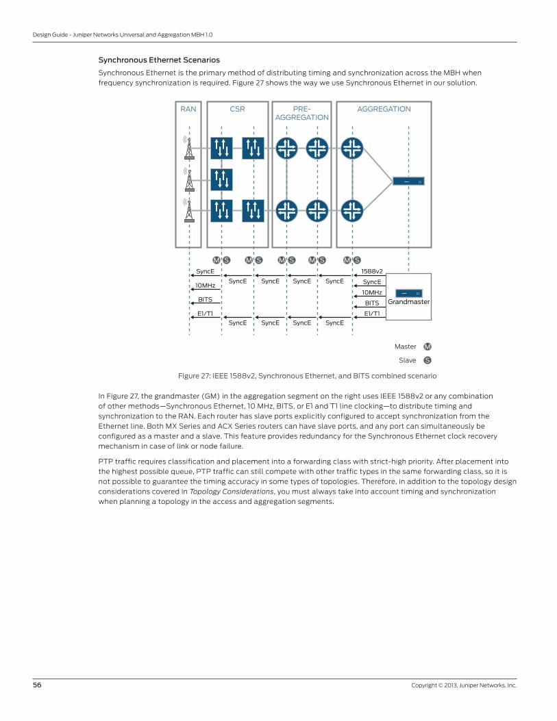
56 Copyright © 2013, Juniper Networks, Inc.
Design Guide - Juniper Networks Universal and Aggregation MBH 1.0
Synchronous Ethernet Scenarios
Synchronous Ethernet is the primary method of distributing timing and synchronization across the MBH when
frequency synchronization is required. Figure 27 shows the way we use Synchronous Ethernet in our solution.
SyncE SyncE SyncE SyncE
RAN CSR PRE-AGGREGATION
AGGREGATION
1588v2
SyncE
10MHz
BITS
E1/T1
SyncE
10MHz
BITS
E1/T1
SyncE SyncE SyncE SyncE
M S M S M S M S M S
Grandmaster
MMaster
Slave S
Figure 27: IEEE 1588v2, Synchronous Ethernet, and BITS combined scenario
In Figure 27, the grandmaster (GM) in the aggregation segment on the right uses IEEE 1588v2 or any combination
of other methods—Synchronous Ethernet, 10 MHz, BITS, or E1 and T1 line clocking—to distribute timing and
synchronization to the RAN. Each router has slave ports explicitly configured to accept synchronization from the
Ethernet line. Both MX Series and ACX Series routers can have slave ports, and any port can simultaneously be
configured as a master and a slave. This feature provides redundancy for the Synchronous Ethernet clock recovery
mechanism in case of link or node failure.
PTP traffic requires classification and placement into a forwarding class with strict-high priority. After placement into
the highest possible queue, PTP traffic can still compete with other traffic types in the same forwarding class, so it is
not possible to guarantee the timing accuracy in some types of topologies. Therefore, in addition to the topology design
considerations covered in Topology Considerations, you must always take into account timing and synchronization
when planning a topology in the access and aggregation segments.
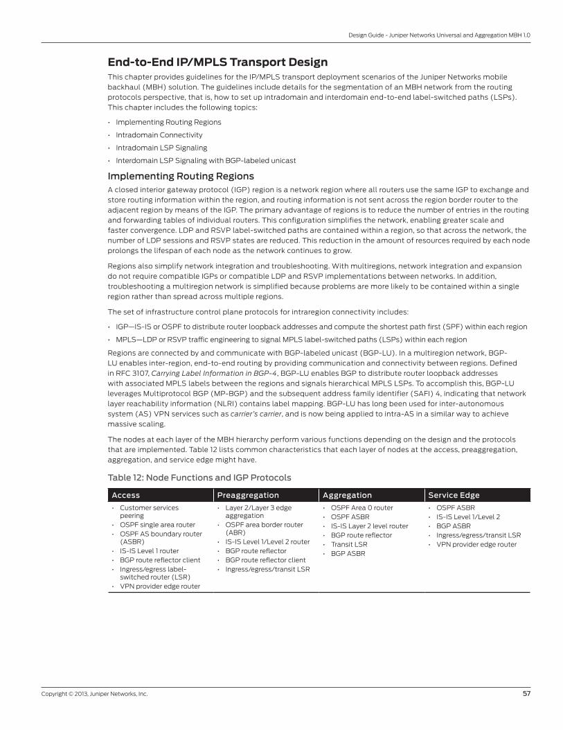
Copyright © 2013, Juniper Networks, Inc. 57
Design Guide - Juniper Networks Universal and Aggregation MBH 1.0
End-to-End IP/MPLS Transport DesignThis chapter provides guidelines for the IP/MPLS transport deployment scenarios of the Juniper Networks mobile
backhaul (MBH) solution. The guidelines include details for the segmentation of an MBH network from the routing
protocols perspective, that is, how to set up intradomain and interdomain end-to-end label-switched paths (LSPs).
This chapter includes the following topics:
• Implementing Routing Regions
• Intradomain Connectivity
• Intradomain LSP Signaling
• Interdomain LSP Signaling with BGP-labeled unicast
Implementing Routing RegionsA closed interior gateway protocol (IGP) region is a network region where all routers use the same IGP to exchange and
store routing information within the region, and routing information is not sent across the region border router to the
adjacent region by means of the IGP. The primary advantage of regions is to reduce the number of entries in the routing
and forwarding tables of individual routers. This configuration simplifies the network, enabling greater scale and
faster convergence. LDP and RSVP label-switched paths are contained within a region, so that across the network, the
number of LDP sessions and RSVP states are reduced. This reduction in the amount of resources required by each node
prolongs the lifespan of each node as the network continues to grow.
Regions also simplify network integration and troubleshooting. With multiregions, network integration and expansion
do not require compatible IGPs or compatible LDP and RSVP implementations between networks. In addition,
troubleshooting a multiregion network is simplified because problems are more likely to be contained within a single
region rather than spread across multiple regions.
The set of infrastructure control plane protocols for intraregion connectivity includes:
• IGP—IS-IS or OSPF to distribute router loopback addresses and compute the shortest path first (SPF) within each region
• MPLS—LDP or RSVP traffic engineering to signal MPLS label-switched paths (LSPs) within each region
Regions are connected by and communicate with BGP-labeled unicast (BGP-LU). In a multiregion network, BGP-
LU enables inter-region, end-to-end routing by providing communication and connectivity between regions. Defined
in RFC 3107, Carrying Label Information in BGP-4, BGP-LU enables BGP to distribute router loopback addresses
with associated MPLS labels between the regions and signals hierarchical MPLS LSPs. To accomplish this, BGP-LU
leverages Multiprotocol BGP (MP-BGP) and the subsequent address family identifier (SAFI) 4, indicating that network
layer reachability information (NLRI) contains label mapping. BGP-LU has long been used for inter-autonomous
system (AS) VPN services such as carrier’s carrier, and is now being applied to intra-AS in a similar way to achieve
massive scaling.
The nodes at each layer of the MBH hierarchy perform various functions depending on the design and the protocols
that are implemented. Table 12 lists common characteristics that each layer of nodes at the access, preaggregation,
aggregation, and service edge might have.
Table 12: Node Functions and IGP Protocols
Access Preaggregation Aggregation Service Edge
• Customer services peering
• OSPF single area router• OSPF AS boundary router
(ASBR)• IS-IS Level 1 router• BGP route reflector client• Ingress/egress label-
switched router (LSR)• VPN provider edge router
• Layer 2/Layer 3 edge aggregation
• OSPF area border router (ABR)
• IS-IS Level 1/Level 2 router• BGP route reflector• BGP route reflector client• Ingress/egress/transit LSR
• OSPF Area 0 router• OSPF ASBR• IS-IS Layer 2 level router• BGP route reflector• Transit LSR• BGP ASBR
• OSPF ASBR• IS-IS Level 1/Level 2• BGP ASBR• Ingress/egress/transit LSR• VPN provider edge router

58 Copyright © 2013, Juniper Networks, Inc.
Design Guide - Juniper Networks Universal and Aggregation MBH 1.0
Intradomain ConnectivityInterior gateway protocols (IGPs) establish a control plane to signal LSPs within a closed IGP region. This topic
discusses segmenting the access and aggregation network to optimize IGP deployment in the MBH network and the
points you should consider when choosing a particular IGP.
IGP Protocol Consideration
In the MBH solution, we place the access and aggregation segments in a common BGP autonomous system that is
divided into IGP regions using IS-IS or OSPF as the IGP. The Juniper Networks solution supports IS-IS and OSPF as the
IGP of choice. However, in very large implementations with complex topologies in the access segment, we recommend
the use of IS-IS. In simpler cases in the access segment, OSPF offers better routing information isolation between
different OSPF areas than IS-IS offers between different IS-IS levels. To understand this difference between OSPF
areas and IS-IS levels, it is necessary to define two new terms with regard to two types of topology at the access
segment: access region and semi-independent domain.
Semi-Independent Domains and Access Regions
An access region is a region in which two access nodes can establish connectivity to each other at the network (IP)
level without traffic passing though the AG 1 node. Two access regions belong to the same semi-independent access
domain if any two access nodes in the regions can establish connectivity to each other at the network level with traffic
passing through the same AG 1 router. (See Figure 28.)
Aggregation Region
SEMI-INDEPENDENTACCESS DOMAIN 1
SEMI-INDEPENDENTACCESS DOMAIN 2
AG 1.1 AG 1.2
AG 1.3
AG 1.4
AG 1.7
AG 1.6 AG 1.5
Access Region 1
Access Region 2
Access Region 1
Access Region 2
Figure 28: Semi-Independent access domains
Figure 28 illustrates an aggregation region that interconnects four access regions in two semi-independent access
domains—1 and 2. Any two access nodes from two different semi-independent access domains can establish
connectivity at the network level with traffic passing through two or more AG 1 nodes. In this example, we assume that
there is no back door connectivity between two semi-independent access domains.
One access region or one semi-independent access domain forms an independent closed OSPF or IS-IS domain.
Although platforms that serve as access nodes in the MBH network are still capable of serving in a broad IGP region
with 250 access nodes, it is not a reasonable arrangement. As the number of prefixes in the access node routing table
increases, more time is required for the IGP protocol to converge after planned topology changes or after changes due
to a failure.
Route Information Isolation in OSPF and IS-IS Protocols
In contrast with IS-IS, the minimal size of a closed IGP region with OSPF is only one access region. With IS-IS, a semi-
independent access domain made up of a number of access regions becomes the minimal size for the closed IGP
region. (See Figure 29.)
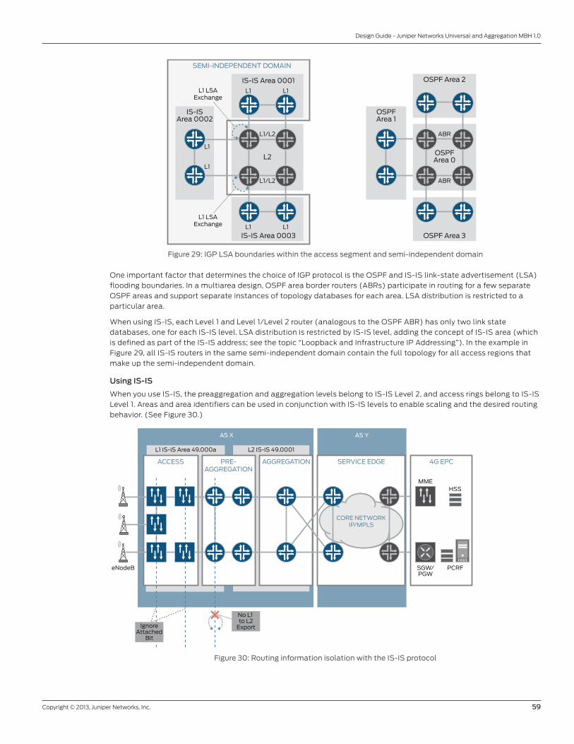
Copyright © 2013, Juniper Networks, Inc. 59
Design Guide - Juniper Networks Universal and Aggregation MBH 1.0
OSPF Area 2
OSPFArea 1
OSPFArea 0
OSPF Area 3
ABR
ABR
L1
L1
SEMI-INDEPENDENT DOMAIN
L2
L1/L2
L1/L2
L1 LSAExchange
L1 LSAExchange L1 L1
L1 L1
IS-IS Area 0001
IS-IS Area 0003
IS-ISArea 0002
Figure 29: IGP LSA boundaries within the access segment and semi-independent domain
One important factor that determines the choice of IGP protocol is the OSPF and IS-IS link-state advertisement (LSA)
flooding boundaries. In a multiarea design, OSPF area border routers (ABRs) participate in routing for a few separate
OSPF areas and support separate instances of topology databases for each area. LSA distribution is restricted to a
particular area.
When using IS-IS, each Level 1 and Level 1/Level 2 router (analogous to the OSPF ABR) has only two link state
databases, one for each IS-IS level. LSA distribution is restricted by IS-IS level, adding the concept of IS-IS area (which
is defined as part of the IS-IS address; see the topic “Loopback and Infrastructure IP Addressing”). In the example in
Figure 29, all IS-IS routers in the same semi-independent domain contain the full topology for all access regions that
make up the semi-independent domain.
Using IS-IS
When you use IS-IS, the preaggregation and aggregation levels belong to IS-IS Level 2, and access rings belong to IS-IS
Level 1. Areas and area identifiers can be used in conjunction with IS-IS levels to enable scaling and the desired routing
behavior. (See Figure 30.)
L1 IS-IS Area 49.000a
AS X AS Y
L2 IS-IS 49.0001
ACCESS SERVICE EDGEPRE-AGGREGATION
AGGREGATION
CORE NETWORKIP/MPLS
IgnoreAttached
Bit
No L1 to L2
Export
eNodeB
MME
SGW/PGW
HSS
PCRF
4G EPC
Figure 30: Routing information isolation with the IS-IS protocol
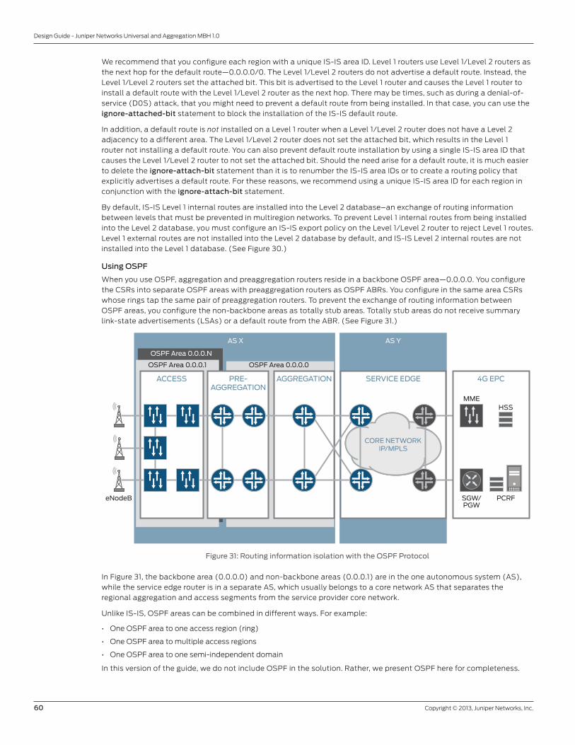
60 Copyright © 2013, Juniper Networks, Inc.
Design Guide - Juniper Networks Universal and Aggregation MBH 1.0
We recommend that you configure each region with a unique IS-IS area ID. Level 1 routers use Level 1/Level 2 routers as
the next hop for the default route—0.0.0.0/0. The Level 1/Level 2 routers do not advertise a default route. Instead, the
Level 1/Level 2 routers set the attached bit. This bit is advertised to the Level 1 router and causes the Level 1 router to
install a default route with the Level 1/Level 2 router as the next hop. There may be times, such as during a denial-of-
service (D0S) attack, that you might need to prevent a default route from being installed. In that case, you can use the
ignore-attached-bit statement to block the installation of the IS-IS default route.
In addition, a default route is not installed on a Level 1 router when a Level 1/Level 2 router does not have a Level 2
adjacency to a different area. The Level 1/Level 2 router does not set the attached bit, which results in the Level 1
router not installing a default route. You can also prevent default route installation by using a single IS-IS area ID that
causes the Level 1/Level 2 router to not set the attached bit. Should the need arise for a default route, it is much easier
to delete the ignore-attach-bit statement than it is to renumber the IS-IS area IDs or to create a routing policy that
explicitly advertises a default route. For these reasons, we recommend using a unique IS-IS area ID for each region in
conjunction with the ignore-attach-bit statement.
By default, IS-IS Level 1 internal routes are installed into the Level 2 database–an exchange of routing information
between levels that must be prevented in multiregion networks. To prevent Level 1 internal routes from being installed
into the Level 2 database, you must configure an IS-IS export policy on the Level 1/Level 2 router to reject Level 1 routes.
Level 1 external routes are not installed into the Level 2 database by default, and IS-IS Level 2 internal routes are not
installed into the Level 1 database. (See Figure 30.)
Using OSPF
When you use OSPF, aggregation and preaggregation routers reside in a backbone OSPF area—0.0.0.0. You configure
the CSRs into separate OSPF areas with preaggregation routers as OSPF ABRs. You configure in the same area CSRs
whose rings tap the same pair of preaggregation routers. To prevent the exchange of routing information between
OSPF areas, you configure the non-backbone areas as totally stub areas. Totally stub areas do not receive summary
link-state advertisements (LSAs) or a default route from the ABR. (See Figure 31.)
OSPF Area 0.0.0.N
AS X AS Y
OSPF Area 0.0.0.0OSPF Area 0.0.0.1
eNodeB
ACCESS SERVICE EDGEPRE-AGGREGATION
AGGREGATION
CORE NETWORKIP/MPLS
MME
SGW/PGW
HSS
PCRF
4G EPC
Figure 31: Routing information isolation with the OSPF Protocol
In Figure 31, the backbone area (0.0.0.0) and non-backbone areas (0.0.0.1) are in the one autonomous system (AS),
while the service edge router is in a separate AS, which usually belongs to a core network AS that separates the
regional aggregation and access segments from the service provider core network.
Unlike IS-IS, OSPF areas can be combined in different ways. For example:
• One OSPF area to one access region (ring)
• One OSPF area to multiple access regions
• One OSPF area to one semi-independent domain
In this version of the guide, we do not include OSPF in the solution. Rather, we present OSPF here for completeness.

Copyright © 2013, Juniper Networks, Inc. 61
Design Guide - Juniper Networks Universal and Aggregation MBH 1.0
Intradomain LSP SignalingTo signal MPLS LSPs within a domain, you can use RSVP or LDP. Taking into account strict requirements for MBH
network resiliency, we strongly recommend that you use RSVP as the universal solution for any topology in the access
and aggregation segments. RSVP provides protection for transport LSPs and rapid convergence in case of a failure.
LDP provides a simple way of setting up a full meshed LSP topology within the IGP region. You can use LDP in some
limited cases. For example, in a hub-and-spoke topology, you might use LDP with OSPF loop-free alternates (LFAs)
to provide protection in the event of a failure. However, this technique does not work for resiliency in ring and partially
meshed topologies.
Deciding on the LSP TopologyIn the preaggregation segment, a full mesh LSP topology is the natural choice within the backbone IGP region—OSPF
backbone area 0.0.0.0 or IS-IS Level 2.
However, in the access segment and within the IGP access region, you can use a full mesh topology, but you need to
take into account the potential complexity and scalability issues that might arise. You have two possible options for
the LSP topology:
• A fully meshed RSVP LSP topology
• A hub-and-spoke RSVP LSP topology
A fully meshed LSP topology in the access region uses LTE mobile networks where IP connectivity between eNodeBs
is required to enable X2 interface communication. A full mesh establishes a continuous LSP protected by MPLS fast
reroute (FRR) and link-node protection between any two nodes within the IGP region. In contrast, the hub-and-spoke
RSVP LSP topology provides better protection against preaggregation AG 1 node failure and the shortest connectivity
path between two eNodeBs to minimize the delay in packet delivery.
The relative complexity of a fully meshed LSP topology can require support of as many as 2*N*(N-1) LSPs in an IGP
region that must be provisioned at zero time implementation. (Here N stands for the number of access nodes in one
IGP region.) You can try to address the problem of complexity by using the RSVP automesh configuration feature or by
using bulk RSVP configuration within the network management system. This approach has not been tested and is not
included as part of this solution.
Scalability can also be an issue with a fully meshed LSP topology. The total number of labels supported by ACX Series
routers that serve as access nodes is 3,000 labels per router. Depending on the exact topology and number of nodes
in one IGP region, it is possible to reach this number. You should carefully calculate transport labels for ingress, egress,
and transit LSPs—including LSPs to remote service edge routers, and service-level labels for MPLS VPNs. A full mesh
LSP topology creates many transit states on CSRs. These transit LSP states exhaust resources, reduce the scalability
of the topology, and restrict the number of CSRs in one IGP region. To avoid all of this complexity and potential
scalability issues, we recommend the hub-and-spoke RSVP LSP topology. In this kind of topology, we build one RSVP
LSP from each CSR to some aggregation routers, specifically Router AG 1.1 and Router AG 1.2.
Interdomain LSP Signaling with BGP-Labeled UnicastAfter you have defined the regions and roles for each router, the regions need a way to create end-to-end connectivity
and enable inter-region communication. Because regions are not configured to share IGP routing information, you
introduce an additional protocol—BGP-LU—to handle interdomain LSP signaling so that PE routers can reach remote
PE routers in other regions.
For inter-region reachability of access nodes, seamless MPLS introduces BGP-labeled unicast (BGP-LU) (RFC 3107)
and hierarchical LSPs. BGP-LU is the label signaling and routing protocol that provides edge-to-edge or PE-to-PE
reachability. The hops of the BGP-LU LSP do not need to be adjacent, just as two neighbors that form a unicast
internal BGP (IBGP) session do not need to be adjacent. Rather, the BGP-LU LSP hops are those routers that
participate in BGP-LU and are in the forwarding path. Transit routers within each region are not required to detect or
participate in BGP-LU—one of the reasons BGP-LU scales so well. (See Figure 32.)

62 Copyright © 2013, Juniper Networks, Inc.
Design Guide - Juniper Networks Universal and Aggregation MBH 1.0
HUB-AND-SPOKE LSP
AS X AS Y
eNodeB
CSR 1.3
ACCESS SERVICE EDGEPRE-AGGREGATION
AGGREGATION
CORE NETWORKIP/MPLS
L2 IS-IS Area 49.0001L1 IS-IS Area 49.000a
HUB-AND-SPOKE LSP
IS-IS Level 1 IS-IS Level 2 Core IGP Domain
RSVP RSVP/LDPFull Mesh RSVPPhysical
Connectivity
BGP-LUEBGP-LUBGP-LU
RR(RFC 3107)
Copy CSR’s loopbacksto inet.3 and redistribute
to BGP-LU protocol
Copy local loopbackto inet.3 and redistribute
to BGP-LU protocol
AG 1.3 AG 2.1CSR 1.2 CSR 1.1 AG 1.1
AG 1.4CSR 1.5 AG 1.2 AG 2.2CSR 1.4
AG 3.1
AG 3.2
PE 1
PE 2
MME
SGW/PGW
HSS
PCRF
4G EPC
HUB-AND-SPOKE LSP
BGP-LU LSP
Figure 32: Establishing an inter-AS LSP with BGP-LU
Figure 32 illustrates an inter-AS LSP with IS-IS as the IGP. The AG 1 routers and the AG 2.1 and AG 2.2 routers form
IBGP-LU peering sessions. The AG 2.1 and AG 2.2 routers act as route reflectors, and the AG 1 routers act as route
reflector clients. The AG 1 routers redistribute the CSR loopback addresses into BGP-LU, and advertise them to the
local route reflectors, which in turn reflect them to AG 1 routers in other preaggregation rings. (See Figure 17.) When the
route reflector readvertises BGP-LU routes, the route reflector does not change the BGP next hop, which is the default
behavior for IBGP route reflection.
At the same time, the AG 2.1 and AG 2.2 routers serve as ASBRs and are peers with multiservice edge routers AG 3.1 and
AG 3.2. To establish peering, you use external BGP (EBGP). Routes are advertised from the preaggregation segment to
the core IGP region, with the next hop pointing to the AG 2.1 and AG 2.2 routers (next-hop-self)—the default behavior
for EBGP.
In the access segment, you do not use BGP-LU. The AG 1 routers have routes to the loopback address of all the CSRs
from IGP advertisements. So to make the CSRs reachable from multiservice edge routers AG 3.1 and AG 3.2, two things
must happen on the AG 1 routers. First, you must configure the AG 1 routers to copy the CSR loopback addresses from
the inet.0 to the inet.3 routing table, so that these loopback addresses are advertised as MPLS-labeled routes. Second,
the AG 1 routers must redistribute these MPLS-labeled routes into BGP-LU. The routers that participate in BGP-LU
peering—AG 2, AG 3.1 and AG 3.2, PE 1 and PE 2—must be configured in a similar way. These routers must redistribute
their local loopback addresses into BGP-LU. This approach makes the AG 2 routers, AG 3 routers, and PE routers
allocate an MPLS label for each BGP-LU MPLS forwarding equivalence class (FEC) that the AG 1 routers advertise in
the local aggregation region, creating the required end-to-end LSP hierarchy.

Copyright © 2013, Juniper Networks, Inc. 63
Design Guide - Juniper Networks Universal and Aggregation MBH 1.0
MPLS Services Design for the 4G LTE ProfileThis chapter includes detailed descriptions of the MPLS services design for the MBH network. The design of the MPLS
services meets the requirements for each of the service profiles—4G and HSPA.
End-to-End Layer 3 VPN DesignThe service model for the 4G LTE mobile network uses a Layer 3 VPN, which meets all service requirements and
provides the necessary connectivity between eNodeBs and the mobile EPC. In this example, you set up end-to-end
Layer 3 VPN services between each access node and remote provider edge (PE) service router using S1-U, S1-MME, and
X2 interfaces. (See Figure 33.)
MME
SGW/PGW
EPC
VLAN S1-MMEVLAN X2 S1-MME
S1-uPE
L3 VPN for S1-MME
L3 VPN for X2
L3 VPN for S1-u
eNode B
eNode B VLAN S1-u
VLAN S1-MMEVLAN X2
VLAN S1-u
LogicalInterface
Physical Port X2
SN SN
IP/MPLSMBH
AN
AN
S1-u
S1-MME
Figure 33: Layer 3 VPN design for the 4G LTE service profile
In addition, you need to provide any-to-any connectivity between access nodes within the same Layer 3 VPN. At the
UNI, you can represent a service through the physical interface, but more commonly you would use a VLAN-tagged
logical interface. To connect an eNodeB to an access node or an EPC to a PE router, you can use an arbitrary unique
VLAN number within the 1 through 4,095 range. The VLAN number has a local meaning within the port of each service
node, so you do not need to synchronize the VLAN number across the MBH network. Service nodes at both ends use
logical interfaces with IPv4 addresses assigned to provide necessary connectivity with the mobile network elements
at the network layer. These logical interfaces are placed into separate routing instances within a service node and, in
this guide, are referred to as VPN routing and forwarding (VRF) or a VRF table. VRF tables have a local meaning and
provide necessary traffic and routing information separation between services within one service node. You assign each
VRF table to one Layer 3 VPN. A Layer 3 VPN has a global meaning across the MBH network that you define with two
characteristics:
• Service label—Provides separation of traffic belonging to different services or VPNs when the logical interface transfers
traffic through the MBH network.
• VRF route target—Unique VPN identifier advertised as an MP-BGP extended community. The VRF route target
manipulates routing information advertised to and from service nodes and places VRF prefixes into the correct VRF table.
In the sample topologies, we use one common Layer 3 VPN for all LTE traffic types. This Layer 3 VPN is easily adapted
to multiple VRFs (one per S1-U, S1-MME, X2, eNodeB).
Figure 34 shows a detailed diagram of the BGP peering sessions between routers in the MBH network. In this example,
we use MP-BGP to signal Layer 3 VPN service labels across the MBH network from the CSRs to the PE routers. To
provide necessary scalability in terms of the number of BGP sessions that the CSR, AG 1, and AG 2 routers need, a
hierarchy of BGP route reflectors is used. AG 1 routers serve as BGP route reflectors for CSRs in the directly connect
access regions, and AG 2 routers serve as BGP route reflectors for the AG 1 routers in the corresponding preaggregation
regions. (See Figure 34.)

64 Copyright © 2013, Juniper Networks, Inc.
Design Guide - Juniper Networks Universal and Aggregation MBH 1.0
L3 VPN
Remote PE
Remote PEAS X AS Y
L2 IS-IS Area 49.0001L1 IS-IS Area 49.000a
eNodeB
CSR 1.3
AG 1.3
AG 1.4CSR 1.5
ACCESS SERVICE EDGEPRE-AGGREGATION
AGGREGATION
CORENETWORK
IP/MPLS
CSR 1.1
IS-IS Level 1 Direct Connection Core IGPDomain
MP-IBGP
IS-IS Level 2
MP-EBGP(RFC 4364)
MP-IBGP
RR(RFC 2547)
RR(RFC 2547)
AG 1.2
AG 2.1CSR 1.2 AG 1.1
AG 2.2
AG 3.1
AG 3.2
PE 1
PE 2CSR 1.4
L3 VPN
LSPLSP
ServiceEdge
MME
SGW/PGW
HSS
PCRF
4G EPC
Figure 34: End-to-end Layer 3 VPN deployment scenarios
In Figure 34, the following mechanisms are used to signal Layer 3 VPN service labels and VRF prefixes from the access
node to the opposite end of the network. This end could be either a remote PE router (to provide S1-connectivity) or
another CSR that has eNodeB connected within the same VRF (to provide X2-connectivity), as shown in Figure 33.
1. The CSR announces a service label and VRF prefixes to the adjacent AG 1 route reflectors with the next hop pointing to its own loopback address.
2. An AG 1 route reflector readvertises the CSR announcement:
• Among other CSRs in the same access ring.
• Among other CSRs in adjacent access rings. There is only one access ring depicted in Figure 34, but in an actual network there are multiple access rings. (See Figure 17.)
• To the AG 2.1 and AG 2.2 routers in the MP-IBGP session.
• To the service edge PE 1 and PE 2 routers in the MP-EBGP (RFC 4364) session. This announcement changes the next hop to its own loopback address, which is the default behavior for EBGP.
Using similar mechanisms, PE routers distribute VRF prefixes and Layer 3 VPN service labels across the MBH network
to CSRs.
1. A PE router announces a service label and VRF prefixes to the AG 1 route reflectors in MP-EBGP (RFC 4364), with the next hop pointing to its own loopback address.
2. An AG 1 route reflector readvertises this announcement to the adjacent CSRs in the MP-IBGP session and changes the next hop to its own loopback address, which is the default behavior for announcements received through EBGP.
At this point, PE routers signal VPN labels in both directions and distribute VRF prefixes from one end of the network to
the other end and vice versa.
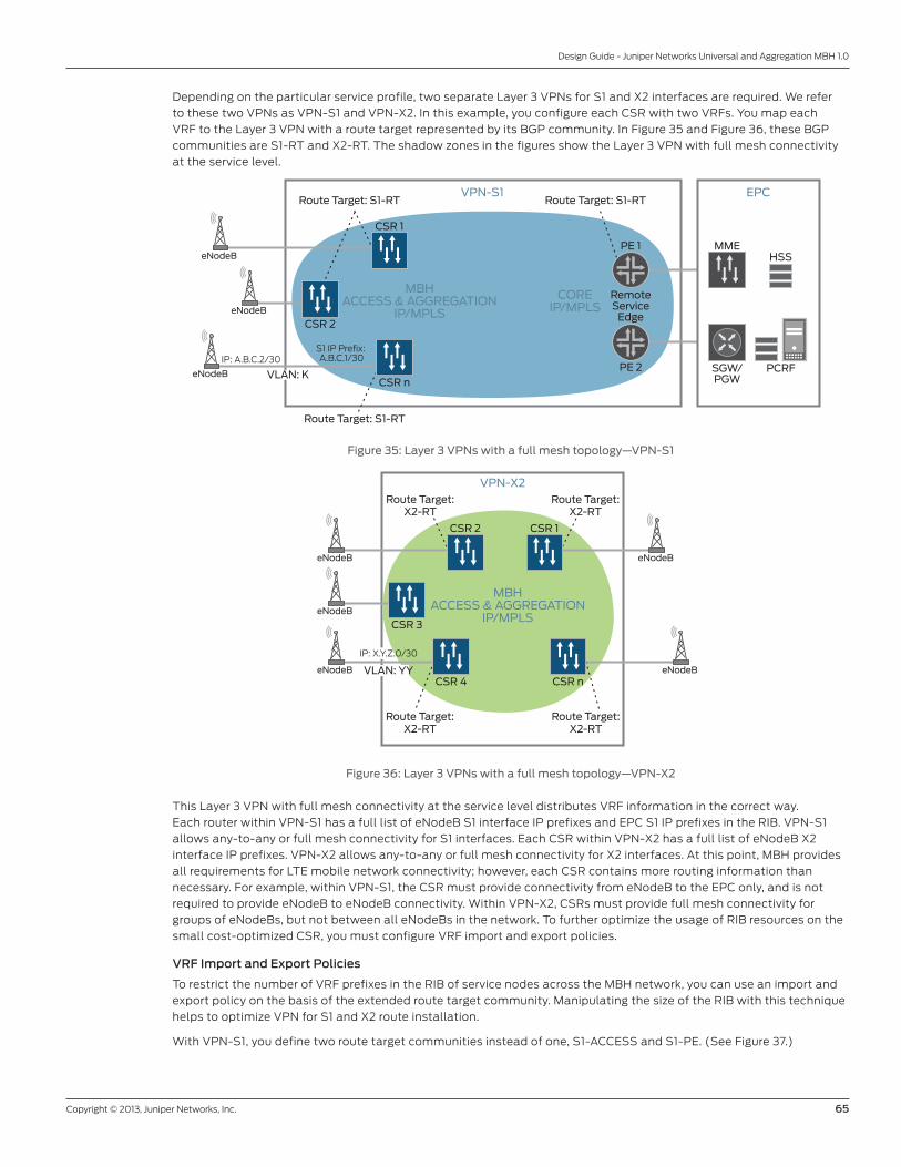
Copyright © 2013, Juniper Networks, Inc. 65
Design Guide - Juniper Networks Universal and Aggregation MBH 1.0
Depending on the particular service profile, two separate Layer 3 VPNs for S1 and X2 interfaces are required. We refer
to these two VPNs as VPN-S1 and VPN-X2. In this example, you configure each CSR with two VRFs. You map each
VRF to the Layer 3 VPN with a route target represented by its BGP community. In Figure 35 and Figure 36, these BGP
communities are S1-RT and X2-RT. The shadow zones in the figures show the Layer 3 VPN with full mesh connectivity
at the service level.
CSR 1
CSR 2
Route Target: S1-RT
S1 IP Prefix: A.B.C.1/30IP: A.B.C.2/30
CSR n
COREIP/MPLS
MBHACCESS & AGGREGATION
IP/MPLSeNodeB
eNodeB
eNodeB
VPN-S1
PE 1
PE 2
RemoteService
Edge
Route Target: S1-RTRoute Target: S1-RT
VLAN: K
MME
SGW/PGW
HSS
PCRF
EPC
Figure 35: Layer 3 VPNs with a full mesh topology—VPN-S1
CSR 2
CSR 3
Route Target:X2-RT
Route Target:X2-RT
Route Target:X2-RT
CSR 4
MBHACCESS & AGGREGATION
IP/MPLSeNodeB
eNodeB
eNodeB eNodeB
VPN-X2Route Target:
X2-RT
eNodeB
CSR 1
CSR nVLAN: YY
IP: X.Y.Z.0/30
Figure 36: Layer 3 VPNs with a full mesh topology—VPN-X2
This Layer 3 VPN with full mesh connectivity at the service level distributes VRF information in the correct way.
Each router within VPN-S1 has a full list of eNodeB S1 interface IP prefixes and EPC S1 IP prefixes in the RIB. VPN-S1
allows any-to-any or full mesh connectivity for S1 interfaces. Each CSR within VPN-X2 has a full list of eNodeB X2
interface IP prefixes. VPN-X2 allows any-to-any or full mesh connectivity for X2 interfaces. At this point, MBH provides
all requirements for LTE mobile network connectivity; however, each CSR contains more routing information than
necessary. For example, within VPN-S1, the CSR must provide connectivity from eNodeB to the EPC only, and is not
required to provide eNodeB to eNodeB connectivity. Within VPN-X2, CSRs must provide full mesh connectivity for
groups of eNodeBs, but not between all eNodeBs in the network. To further optimize the usage of RIB resources on the
small cost-optimized CSR, you must configure VRF import and export policies.
VRF Import and Export Policies
To restrict the number of VRF prefixes in the RIB of service nodes across the MBH network, you can use an import and
export policy on the basis of the extended route target community. Manipulating the size of the RIB with this technique
helps to optimize VPN for S1 and X2 route installation.
With VPN-S1, you define two route target communities instead of one, S1-ACCESS and S1-PE. (See Figure 37.)

66 Copyright © 2013, Juniper Networks, Inc.
Design Guide - Juniper Networks Universal and Aggregation MBH 1.0
CSR 1
CSR 2
VLAN: K
IP: A.B.C.0/30
CSR n
COREIP/MPLS
MBHACCESS & AGGREGATION
IP/MPLSeNodeB
eNodeB
eNodeB
VPN-S1
PE 1
PE 2
RemoteService
Edge
Import Community: S-AccessExport Community: S1-PE
Import Community: S1-PEExport Community: S1-Access
Import Community: S1-PEExport Community: S1-Access
MME
SGW/PGW
HSS
PCRF
EPC
Figure 37: VRF import and export policies for S1 Layer 3 VPN
In Figure 37, each CSR and PE router advertises VRF prefixes and installs BGP routes in different ways. Each CSR
advertises VRF prefixes with the S1-ACCESS BGP community, and installs only the BGP routes received with the S1-
PE community into its VRF table. In contrast, each PE router advertises VRF prefixes with the S1-PE BGP community
and installs only BGP routes received with the S1-ACCESS community into its S1 VRF-table. Thus, we build a point-to-
multipoint Layer 3 VPN, topology where CSRs contain only S1 prefixes from the PE router and the PE router has a full
list of all S1 prefixes from all CSRs. The three shadow zones in Figure 37 show the Layer 3 VPN-S1 with hub-and-spoke
connectivity at the service level.
With VPN X2, which is somewhat different from the VPN-S1 service, you use the same import and export policies based
on the extended route target community. However, you map the community name to a geographical location or to the
indexing group of an eNodeB. The eNodeB defines the group of eNodeBs requiring X2 connectivity from one eNodeB to
another. (See Figure 38.)
CSR 2
CSR 3
VLAN: YYCSR 4
eNodeB
eNodeB eNodeB
CSR 1
CSR n
eNodeB eNodeB
MBHACCESS & AGGREGATION
IP/MPLS
IP: X.Y.Z.0/30
VPN-X2
Import Community: X2-ZONE-BExport Community: X2-ZONE-B
Import Community: X2-ZONE-AExport Community: X2-ZONE-A
Figure 38: Using VRF import and export policies for X2 Layer 3 VPN
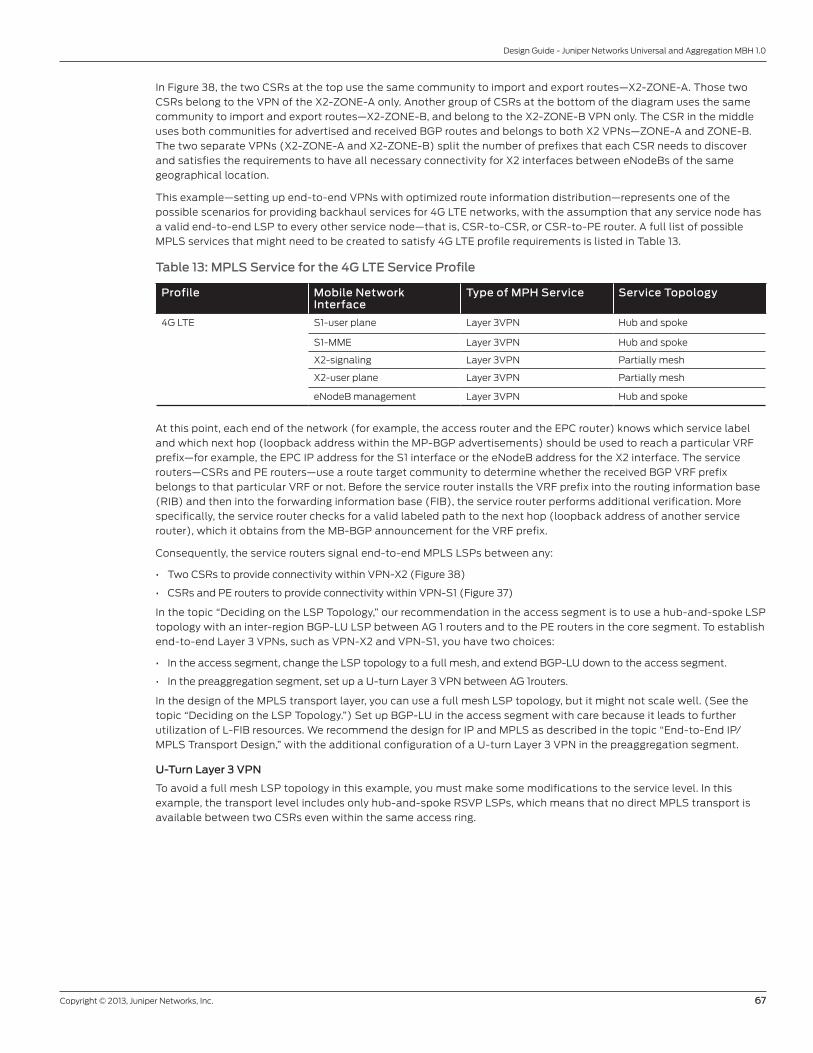
Copyright © 2013, Juniper Networks, Inc. 67
Design Guide - Juniper Networks Universal and Aggregation MBH 1.0
In Figure 38, the two CSRs at the top use the same community to import and export routes—X2-ZONE-A. Those two
CSRs belong to the VPN of the X2-ZONE-A only. Another group of CSRs at the bottom of the diagram uses the same
community to import and export routes—X2-ZONE-B, and belong to the X2-ZONE-B VPN only. The CSR in the middle
uses both communities for advertised and received BGP routes and belongs to both X2 VPNs—ZONE-A and ZONE-B.
The two separate VPNs (X2-ZONE-A and X2-ZONE-B) split the number of prefixes that each CSR needs to discover
and satisfies the requirements to have all necessary connectivity for X2 interfaces between eNodeBs of the same
geographical location.
This example—setting up end-to-end VPNs with optimized route information distribution—represents one of the
possible scenarios for providing backhaul services for 4G LTE networks, with the assumption that any service node has
a valid end-to-end LSP to every other service node—that is, CSR-to-CSR, or CSR-to-PE router. A full list of possible
MPLS services that might need to be created to satisfy 4G LTE profile requirements is listed in Table 13.
Table 13: MPLS Service for the 4G LTE Service Profile
Profile Mobile Network Interface
Type of MPH Service Service Topology
4G LTE S1-user plane Layer 3VPN Hub and spoke
S1-MME Layer 3VPN Hub and spoke
X2-signaling Layer 3VPN Partially mesh
X2-user plane Layer 3VPN Partially mesh
eNodeB management Layer 3VPN Hub and spoke
At this point, each end of the network (for example, the access router and the EPC router) knows which service label
and which next hop (loopback address within the MP-BGP advertisements) should be used to reach a particular VRF
prefix—for example, the EPC IP address for the S1 interface or the eNodeB address for the X2 interface. The service
routers—CSRs and PE routers—use a route target community to determine whether the received BGP VRF prefix
belongs to that particular VRF or not. Before the service router installs the VRF prefix into the routing information base
(RIB) and then into the forwarding information base (FIB), the service router performs additional verification. More
specifically, the service router checks for a valid labeled path to the next hop (loopback address of another service
router), which it obtains from the MB-BGP announcement for the VRF prefix.
Consequently, the service routers signal end-to-end MPLS LSPs between any:
• Two CSRs to provide connectivity within VPN-X2 (Figure 38)
• CSRs and PE routers to provide connectivity within VPN-S1 (Figure 37)
In the topic “Deciding on the LSP Topology,” our recommendation in the access segment is to use a hub-and-spoke LSP
topology with an inter-region BGP-LU LSP between AG 1 routers and to the PE routers in the core segment. To establish
end-to-end Layer 3 VPNs, such as VPN-X2 and VPN-S1, you have two choices:
• In the access segment, change the LSP topology to a full mesh, and extend BGP-LU down to the access segment.
• In the preaggregation segment, set up a U-turn Layer 3 VPN between AG 1routers.
In the design of the MPLS transport layer, you can use a full mesh LSP topology, but it might not scale well. (See the
topic “Deciding on the LSP Topology.”) Set up BGP-LU in the access segment with care because it leads to further
utilization of L-FIB resources. We recommend the design for IP and MPLS as described in the topic “End-to-End IP/
MPLS Transport Design,” with the additional configuration of a U-turn Layer 3 VPN in the preaggregation segment.
U-Turn Layer 3 VPN
To avoid a full mesh LSP topology in this example, you must make some modifications to the service level. In this
example, the transport level includes only hub-and-spoke RSVP LSPs, which means that no direct MPLS transport is
available between two CSRs even within the same access ring.

68 Copyright © 2013, Juniper Networks, Inc.
Design Guide - Juniper Networks Universal and Aggregation MBH 1.0
AS X AS Y
L2 IS-IS Area 49.0001L1 IS-IS Area 49.000a
eNodeB
CSR 1.3
AG 1.3
AG 1.4CSR 1.5
ACCESS SERVICE EDGEPRE-AGGREGATION
AGGREGATION
LSP INFRASTRUCTURE
SERVICE LAYER
CORENETWORK
IP/MPLS
CSR 1.1
IS-IS Level 1 IS-IS Level 2 Direct Connection Core IGPDomain
MP-IBGP MP-EBGP
RR(RFC 2547)
AG 1.2
AG 2.1CSR 1.2 AG 1.1
AG 2.2
AG 3.1
AG 3.2
PE 1
PE 2CSR 1.4
Default
NHS
MME
SGW/PGW
HSS
PCRF
4G EPC
BGP-LU LSP
VRF IP-lookup
U-turnL3 VRF
L3 VPN
H&S RSVP LSP
L3 VPN
Figure 39: End-to-end Layer 3 VRF deployment scenarios with U-turn VRF
To overcome this obstacle, you configure a special U-turn VRF (with the same route target) on the loopback interface
of the AG 1 routers. (See Figure 39.) In addition, you configure the AG 1 route reflector to slightly modify the MP-
BGP behavior so that no actual reflection happens within the access region. Instead, you configure the next-hop-self attribute so that a default VRF route is announced by the AG 1 routers to the CSRs. This modification results in
significant reduction of used label and prefix spaces in the RIB and FIB tables of the CSRs and leads eventually to
faster convergence during link or node failure in the access region.
IP/MPLS Transport and Service Full PictureFor the sake of completeness, note how the full protocol stack looks after we put together the MPLS transport and
service portions of the solution. There are two possible scenarios: CSR-to-PE router connectivity and CSR-to-CSR
connectivity. (See Figure 40 and Figure 41, respectively.)
Figure 40 illustrates the full protocol stack and actions taken with MPLS labels when a CSR forwards an MPLS packet
and that packet travels across the network to a PE router (CSR-to-PE router).

Copyright © 2013, Juniper Networks, Inc. 69
Design Guide - Juniper Networks Universal and Aggregation MBH 1.0
AS X AS Y
L2 IS-IS Area 49.0001L1 IS-IS Area 49.000a
eNodeB
CSR 1.3
AG 1.3
AG 1.4CSR 1.5
ACCESS SERVICE EDGE
DATA FLOW
PRE-AGGREGATION
AGGREGATION
CORE NETWORKIP/MPLS
IS-IS Level 1
PhysicalConnectivity
Full MeshRSVPRSVP RSVP / LDP
Core IGP Domain
MP-IBGP
U-turnL3 VRF
MP-EBGP
RR(RFC 2547)
RR(RFC 3107)
AG 1.2
AG 2.1CSR 1.2 CSR 1.1 AG 1.1
AG 2.2
AG 3.1
AG 3.2
PE 1
PE 2CSR 1.4
L3 VPNL3 VPN
Default
NHS
EBGP-LUBGP-LU BGP-LU
BGP-LU LSPH&S RSVP LSP
Copy CSR’s Io.0 addressto inet 3 and redistribute
to BGP-LU protocol
Copy local Io.0 addressto inet 3 and redistribute
to BGP-LU protocol
IS-IS Level 2
L3 VPN
BGP-L
push RSVP-L
L3 VPN
BGP-L
pop RSVP-L
L3 VPN
BGP-L
push
swap
RSVP-L
L3 VPN
BGP-L
swap RSVP-L
L3 VPN
BGP-L
pop
pop
RSVP-L
push L3 VPN
RSVP-Lpush push
L3 VPN
RSVP-Lpop
L3 VPN
BGP-Lswap
pop L3 VPN
VRF IP-lookup
pop/push
4G EPC
MME
SGW/PGW
HSS
PCRF
Figure 40: End-to-end Layer 3 VPN and data flow for eNodeB to 4G EPC connectivity
In Figure 40, the CSR must push a minimum of two labels—a Layer 3 VPN service label (L3 VPN) and a transport label
(RSVP-L) for the intraregion LSP. The Layer 3 VPN service label defines the endpoints across the access, aggregation,
and core network, and routers do not swap this label unless the packet reaches the next service router.
The RSVP transport label defines packet forwarding within the IGP routing region. Service routers and region boundary
routers push or pop the RSVP transport label, and transport nodes swap the RSVP transport label.
The BGP-LU label provides reachability between routing regions, domains, and autonomous systems. It is pushed or
popped at the service node and swapped at the ABR/ASBR nodes.
Figure 41 illustrates the full protocol stack and actions taken with MPLS labels when a CSR forwards an MPLS packet
and that packet travels across the network to another CSR belonging to a different preaggregation region across an
end-to-end Layer 3 VPN-X2 connection (CSR to CSR).

70 Copyright © 2013, Juniper Networks, Inc.
Design Guide - Juniper Networks Universal and Aggregation MBH 1.0
L1 IS-IS Area 49.000bL1 IS-IS Area 49.000a
eNodeB
DATA FLOW
eNodeB
IS-IS Level 1Area N
IS-IS Level 2Area G
IS-IS Level 1Area H
MP-IBGPMP-IBGPMP-IBGP
RR(RFC 2547)
RR(RFC 2547)
PRE-AGGREGATION
CSR 1.3
CSR 1.5
ACCESS
CSR 1.2 CSR 1.1
ACCESS
CSR 1 CSR 2
CSR 5
CSR 3
AG 1.3AG 1.1
AG 1.4AG 1.2CSR 1.4 CSR 4
L3 VPN
RSVP-Lpush
push L3 VPN
RSVP-Lpop
L3 VPN
RSVP-Lpush
pop/push L3 VPN
RSVP-Lpop
pop L3 VPNL3 VPNpop/push
VRF IP-lookup
LSP LSPLSP
L3 VPNL3 VPN U-turnL3 VRF
Figure 41: End-to-end Layer 3 VPN and data flow for eNodeB to eNodeB connectivity
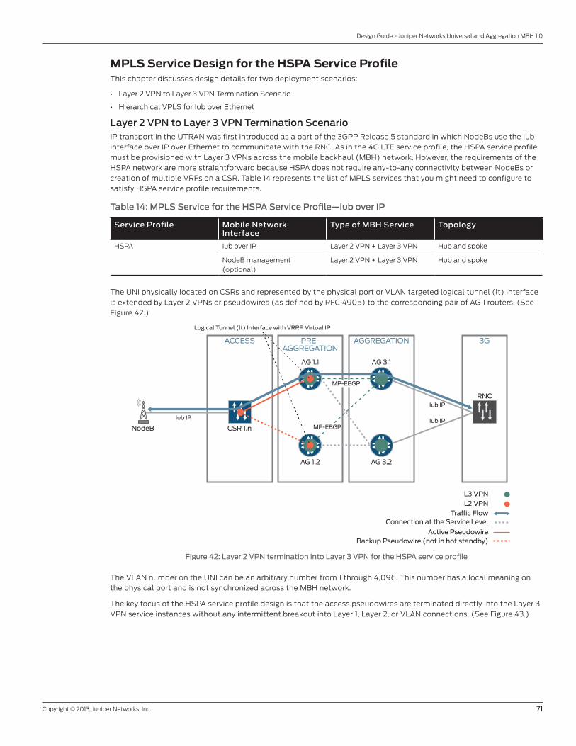
Copyright © 2013, Juniper Networks, Inc. 71
Design Guide - Juniper Networks Universal and Aggregation MBH 1.0
MPLS Service Design for the HSPA Service ProfileThis chapter discusses design details for two deployment scenarios:
• Layer 2 VPN to Layer 3 VPN Termination Scenario
• Hierarchical VPLS for Iub over Ethernet
Layer 2 VPN to Layer 3 VPN Termination Scenario IP transport in the UTRAN was first introduced as a part of the 3GPP Release 5 standard in which NodeBs use the Iub
interface over IP over Ethernet to communicate with the RNC. As in the 4G LTE service profile, the HSPA service profile
must be provisioned with Layer 3 VPNs across the mobile backhaul (MBH) network. However, the requirements of the
HSPA network are more straightforward because HSPA does not require any-to-any connectivity between NodeBs or
creation of multiple VRFs on a CSR. Table 14 represents the list of MPLS services that you might need to configure to
satisfy HSPA service profile requirements.
Table 14: MPLS Service for the HSPA Service Profile—Iub over IP
Service Profile Mobile Network Interface
Type of MBH Service Topology
HSPA Iub over IP Layer 2 VPN + Layer 3 VPN Hub and spoke
NodeB management(optional)
Layer 2 VPN + Layer 3 VPN Hub and spoke
The UNI physically located on CSRs and represented by the physical port or VLAN targeted logical tunnel (lt) interface
is extended by Layer 2 VPNs or pseudowires (as defined by RFC 4905) to the corresponding pair of AG 1 routers. (See
Figure 42.)
NodeB CSR 1.n
RNC
3GACCESS PRE-AGGREGATION
AGGREGATION
AG 1.2
AG 1.1 AG 3.1
Iub IP
Logical Tunnel (lt) Interface with VRRP Virtual IP
AG 3.2
Iub IP
Iub IP
L3 VPNL2 VPN
Trac FlowConnection at the Service Level
MP-EBGP
Active PseudowireBackup Pseudowire (not in hot standby)
MP-EBGP
Figure 42: Layer 2 VPN termination into Layer 3 VPN for the HSPA service profile
The VLAN number on the UNI can be an arbitrary number from 1 through 4,096. This number has a local meaning on
the physical port and is not synchronized across the MBH network.
The key focus of the HSPA service profile design is that the access pseudowires are terminated directly into the Layer 3
VPN service instances without any intermittent breakout into Layer 1, Layer 2, or VLAN connections. (See Figure 43.)
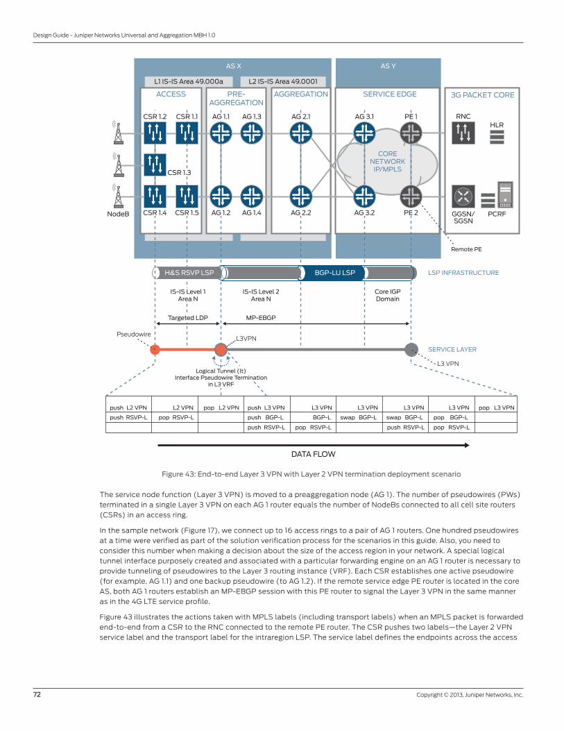
72 Copyright © 2013, Juniper Networks, Inc.
Design Guide - Juniper Networks Universal and Aggregation MBH 1.0
Remote PE
AS X AS Y
L2 IS-IS Area 49.0001L1 IS-IS Area 49.000a
NodeB
ACCESS SERVICE EDGEPRE-AGGREGATION
AGGREGATION
CORENETWORK
IP/MPLS
DATA FLOW
push L2 VPN
push
push
pushRSVP-L
L2 VPN
pop RSVP-L
L3 VPN
BGP-L
pop L2 VPN L3 VPN
BGP-L
push RSVP-L
swap swap
L3 VPN
BGP-L
pop RSVP-L
L3 VPN
BGP-L
push RSVP-L
L3 VPN
BGP-L
pop
pop
L3 VPNpop
RSVP-L
IS-IS Level 2Area N
MP-EBGP
Core IGPDomain
AG 1.2
AG 2.1CSR 1.2 AG 1.1
AG 2.2
AG 3.1
AG 3.2
PE 1
PE 2CSR 1.4
AG 1.3
AG 1.4
IS-IS Level 1Area N
Targeted LDP
RNC
GGSN/SGSN
HLR
PCRF
3G PACKET CORE
CSR 1.1
CSR 1.3
CSR 1.5
L3VPN
BGP-LU LSPH&S RSVP LSP
L3 VPN
Pseudowire
Logical Tunnel (lt)Interface Pseudowire Termination
in L3 VRF
LSP INFRASTRUCTURE
SERVICE LAYER
Figure 43: End-to-end Layer 3 VPN with Layer 2 VPN termination deployment scenario
The service node function (Layer 3 VPN) is moved to a preaggregation node (AG 1). The number of pseudowires (PWs)
terminated in a single Layer 3 VPN on each AG 1 router equals the number of NodeBs connected to all cell site routers
(CSRs) in an access ring.
In the sample network (Figure 17), we connect up to 16 access rings to a pair of AG 1 routers. One hundred pseudowires
at a time were verified as part of the solution verification process for the scenarios in this guide. Also, you need to
consider this number when making a decision about the size of the access region in your network. A special logical
tunnel interface purposely created and associated with a particular forwarding engine on an AG 1 router is necessary to
provide tunneling of pseudowires to the Layer 3 routing instance (VRF). Each CSR establishes one active pseudowire
(for example, AG 1.1) and one backup pseudowire (to AG 1.2). If the remote service edge PE router is located in the core
AS, both AG 1 routers establish an MP-EBGP session with this PE router to signal the Layer 3 VPN in the same manner
as in the 4G LTE service profile.
Figure 43 illustrates the actions taken with MPLS labels (including transport labels) when an MPLS packet is forwarded
end-to-end from a CSR to the RNC connected to the remote PE router. The CSR pushes two labels—the Layer 2 VPN
service label and the transport label for the intraregion LSP. The service label defines the endpoints across the access

Copyright © 2013, Juniper Networks, Inc. 73
Design Guide - Juniper Networks Universal and Aggregation MBH 1.0
region. AG 1 routers apply a pop action to the Layer 2 VPN service label, push the new Layer 3 VPN service label, and
send the packet end-to-end through the interdomain LSP signaled with BGP-LU. Finally, the Layer 3 VPN service label
is popped by the remote PE router, and the native IP packet is forwarded to the mobile network RNC or packet core.
Although this scenario is positioned for the HSPA service profile, it can easily be expanded for 4G LTE networks. Within
the existing set of features, each of the 4G LTE services must be placed into a separate Layer 3 VPN and carried with
a separate pseudowire. However, inconvenience in the number of pseudowires provisioned for each AG 1 router is such
that we do not recommend this method for the primary scenario of the 4G LTE service profile.
Hierarchical VPLS for Iub over EthernetThe service architecture of hierarchical VPLS over Iub for the HSPA mobile network—UMTS Terrestrial Radio Access
Network (UTRAN) over Ethernet—is similar to what was described in the HSPA Iub over IP scenarios. However, inter-AS
Layer 3 VPN is changed to inter-AS VPLS. Table 15 summarizes the MPLS services that you need to configure to satisfy
the requirements of the HSPA service profile.
Table 15: HSPA Services Iub over Ethernet Layer 2 VPN
Service Profile Mobile Network Interface
Type of MBH Service Topology
HSPA Iub over Ethernet H-VPLS Hub and spoke
The UNI physically located on CSRs and represented by the physical port or VLAN targeted logical interface, is
extended by Layer 2 VPNs or pseudowires to the corresponding pair of AG 1 routers. (See draft-martini-l2circuit-encap-
mpls.11.txt. Also, see Figure 44.)
NodeB
RNC
3GACCESS CORE
AG 1.2
AG 1.1 AG 3.1
Iub Ethernet
VPLS Hub with Mesh Groups
AG 3.2
PRE-AGGREGATION
T-LDP
T-LDP
Iub Ethernet
L2 VPNVPLS Instance
Active PseudowireBackup Pseudowire (Standby)
Tra�c FlowConnection at the Service Level
Iub Ethernet
Figure 44: H-VPLS service model for the HSPA service profile
The VLAN number on the UNI can be an arbitrary number from 1 through 4,096. This number has a local meaning
on the physical port and is not synchronized across the MBH network. The key focus of this design is that the access
pseudowires are terminated directly into the VPLS service instances without any intermittent breakout at the physical
layer or data link layer, or at VLAN connections.
A VPLS instance is a concept similar to a Layer 3 routing instance (VRF) defined in the topic “End-to-End Layer 3 VPN
Design.” A VPLS instance is treated as a virtual bridge domain or a virtual switch with its own Layer 2 forwarding table
within a service node to provide a necessary service separation within the node. VLAN-tagged logical interfaces (UNIs)
and Layer 2 pseudowires (NNIs) represent the interfaces of this virtual switch.
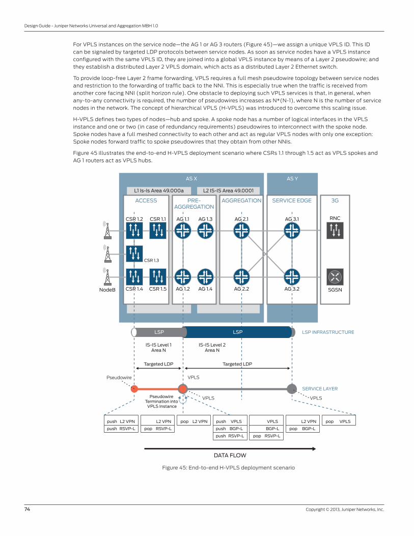
74 Copyright © 2013, Juniper Networks, Inc.
Design Guide - Juniper Networks Universal and Aggregation MBH 1.0
For VPLS instances on the service node—the AG 1 or AG 3 routers (Figure 45)—we assign a unique VPLS ID. This ID
can be signaled by targeted LDP protocols between service nodes. As soon as service nodes have a VPLS instance
configured with the same VPLS ID, they are joined into a global VPLS instance by means of a Layer 2 pseudowire; and
they establish a distributed Layer 2 VPLS domain, which acts as a distributed Layer 2 Ethernet switch.
To provide loop-free Layer 2 frame forwarding, VPLS requires a full mesh pseudowire topology between service nodes
and restriction to the forwarding of traffic back to the NNI. This is especially true when the traffic is received from
another core facing NNI (split horizon rule). One obstacle to deploying such VPLS services is that, in general, when
any-to-any connectivity is required, the number of pseudowires increases as N*(N-1), where N is the number of service
nodes in the network. The concept of hierarchical VPLS (H-VPLS) was introduced to overcome this scaling issue.
H-VPLS defines two types of nodes—hub and spoke. A spoke node has a number of logical interfaces in the VPLS
instance and one or two (in case of redundancy requirements) pseudowires to interconnect with the spoke node.
Spoke nodes have a full meshed connectivity to each other and act as regular VPLS nodes with only one exception:
Spoke nodes forward traffic to spoke pseudowires that they obtain from other NNIs.
Figure 45 illustrates the end-to-end H-VPLS deployment scenario where CSRs 1.1 through 1.5 act as VPLS spokes and
AG 1 routers act as VPLS hubs.
AS X AS Y
L2 IS-IS Area 49.0001L1 Is-Is Area 49.000a
NodeB
CSR 1.3
AG 1.3
AG 1.4CSR 1.5
ACCESS SERVICE EDGEPRE-AGGREGATION
IS-IS Level 1Area N
IS-IS Level 2Area N
Targeted LDP
AG 1.2
AG 2.1CSR 1.2 CSR 1.1 AG 1.1
AG 2.2
AG 3.1
AG 3.2CSR 1.4
DATA FLOW
Pseudowire Termination into
VPLS Instance
AGGREGATION
Targeted LDP
VPLS
BGP-L
push RSVP-L
push
push VPLS
BGP-L
pop RSVP-L
push L2 VPN
RSVP-Lpush
L2 VPN
BGP-Lpop
pop L2 VPN pop VPLSL2 VPN
RSVP-Lpop
RNC
SGSN
3G
VPLS
VPLSVPLS
Pseudowire
LSPLSP LSP INFRASTRUCTURE
SERVICE LAYER
Figure 45: End-to-end H-VPLS deployment scenario

Copyright © 2013, Juniper Networks, Inc. 75
Design Guide - Juniper Networks Universal and Aggregation MBH 1.0
In Figure 45, we configure targeted LDP to signal the pseudowire service labels and the VPLS ID. Each CSR establishes
one active pseudowire to Router AG 1.1 and one backup standby pseudowire to Router AG 1.2. The number of
pseudowires terminated in a single VPLS on each AG 1 router equals the number of NodeBs in each access region
connected to the corresponding AG 1 router, plus pseudowires from remote PE routers. Because there is no traffic
between the AG 1 routers, there is no need to signal pseudowires between the AG 1 routers—except for pairs of AG 1
routers connected to the same access regions. This exception leads to another level of hierarchy represented by PE
routers that act as hub nodes, with the AG 1 routers as spokes.
Unlike Layer 3 VPNs, no tunneling is required to terminate pseudowires in a VPLS instance for those deployment
scenarios, because a special type of label-switched interface (LSI) is used instead of the logical tunnel interface. To set
up H-VPLS, mesh groups within the VPLS instance configuration on AG 1 and AG 3 routers are used.
The consistency of the switching path across the network is provided by the pseudowire backup protocol on the one
hand and the MAC learning process on the other hand. As soon as an active pseudowire goes down, the LSI within
a VPLS instance goes down and triggers the MAC flush event. This event is advertised to adjacent VPLS routers by
means of a flush type, length, and value (TLV) frame. At the next moment, traffic switches over to the second AG 1
router based on the MAC relearning process discussed in more detail in the “Pseudowire Redundancy for the HSPA
Service” topic.
Figure 45 also illustrates actions taken with MPLS labels (including transport labels) when an MPLS packet is
forwarded end-to-end from an access to the RNC connected to the remote PE router. The CSR pushes two labels:
the Layer 2 VPN service label and the transport label for the intraregion LSP. The service label defines the endpoints
across the access region. An AG 1 router applies a pop action to the Layer 2 VPN service label, pushes a new VPLS
service label, and sends the packet end-to-end through the interdomain LSP signaled with BGP-LU. Finally, the VPLS
service label is popped by the remote PE router, and a native Ethernet frame is forwarded to the mobile network RNC
or packet core.
In general, this deployment scenario applies to the 4G LTE service profile. We do not recommend that you use end-
to-end H-VPLS as the primary backhaul service for LTE traffic. However, if you are interested in H-VPLS in your 4G LTE
network, add the following steps to your MPLS service-level design:
• Activate local switching on the VPLS hub to allow connectivity between eNodeBs over the X2 interface.
• Add additional pseudowires for X2 connectivity from the CSRs to the AG 1 routers if necessary.
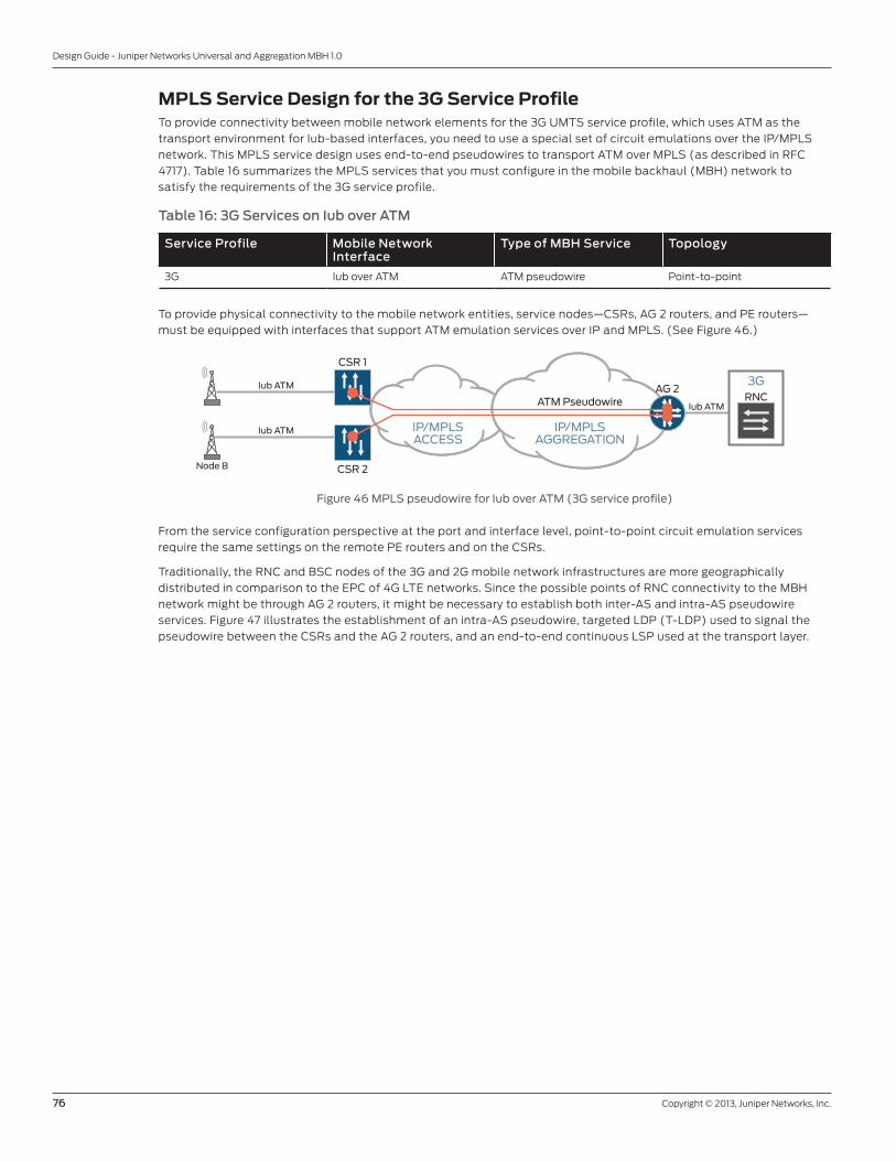
76 Copyright © 2013, Juniper Networks, Inc.
Design Guide - Juniper Networks Universal and Aggregation MBH 1.0
MPLS Service Design for the 3G Service ProfileTo provide connectivity between mobile network elements for the 3G UMTS service profile, which uses ATM as the
transport environment for Iub-based interfaces, you need to use a special set of circuit emulations over the IP/MPLS
network. This MPLS service design uses end-to-end pseudowires to transport ATM over MPLS (as described in RFC
4717). Table 16 summarizes the MPLS services that you must configure in the mobile backhaul (MBH) network to
satisfy the requirements of the 3G service profile.
Table 16: 3G Services on Iub over ATM
Service Profile Mobile Network Interface
Type of MBH Service Topology
3G Iub over ATM ATM pseudowire Point-to-point
To provide physical connectivity to the mobile network entities, service nodes—CSRs, AG 2 routers, and PE routers—
must be equipped with interfaces that support ATM emulation services over IP and MPLS. (See Figure 46.)
Iub ATM
IP/MPLSAGGREGATION
IP/MPLSACCESS
ATM Pseudowire
3GIub ATM
Iub ATM
Node B
CSR 1
RNCAG 2
CSR 2
Figure 46 MPLS pseudowire for Iub over ATM (3G service profile)
From the service configuration perspective at the port and interface level, point-to-point circuit emulation services
require the same settings on the remote PE routers and on the CSRs.
Traditionally, the RNC and BSC nodes of the 3G and 2G mobile network infrastructures are more geographically
distributed in comparison to the EPC of 4G LTE networks. Since the possible points of RNC connectivity to the MBH
network might be through AG 2 routers, it might be necessary to establish both inter-AS and intra-AS pseudowire
services. Figure 47 illustrates the establishment of an intra-AS pseudowire, targeted LDP (T-LDP) used to signal the
pseudowire between the CSRs and the AG 2 routers, and an end-to-end continuous LSP used at the transport layer.

Copyright © 2013, Juniper Networks, Inc. 77
Design Guide - Juniper Networks Universal and Aggregation MBH 1.0
RNC
3G
L2 IS-IS Area 49.0001L1 Is-Is Area 49.000a
NodeB
CSR 1.3
AG 1.3
AG 1.4CSR 1.5
ACCESS
DATA FLOW
PRE-AGGREGATION
AGGREGATION
IS-IS Level 1Area N
IS-IS Level 2Area G
LDP-DOD
LSP
AG 1.2
AG 2.1CSR 1.1 AG 1.1
AG 2.2CSR 1.4
LSPLDP Tunneling
Targeted LDP
CSR 1.2
ATMATM
ATM PW3
LSP INFRASTRUCTURE
SERVICE LAYER
pop L2 VPNL2 VPN
BGP-L
pop RSVP-L
pop
L2 VPN
LDP-DOD
push RSVP-L
push
push L2 VPN
LDP-DOD
pop RSVP-L
L2 VPN
BGP-L
push RSVP-L
swap
Figure 47: End-to-End ATM and TDM pseudowire deployment scenario
To provide a true end-to-end LSP, LDP downstream-on-demand is used (LDP DOD RFC 5036). LDP DOD is configured
on the CSRs and AG 1 routers, enabling the CSR to resolve the loopback address of the remote edge service router with
a labeled path. The CSR requests a transport label for the loopback address of only those service routers to which
the 3G RNC is connected—the AG 2 router in our example—thus preserving the scalability of the CSRs. By design, the
CSRs in the access segment do not have routing information to reach routers in other segments. (See the topic “Using
OSPF.”) However, this information is required to establish T-LDP sessions with AG 2 routers and to install an end-to-
end transport LSP into the forwarding table of the CSR. This restriction can be overcome by the addition, on the CSR,
of a static route that points to the loopback address of the AG 2 router.
Note: Do not use a default or summarized route on the CSR, because LDP-DOD does not install an end-to-end LSP
using those types of routes.
Figure 47 illustrates actions taken with MPLS labels (including transport labels) when an MPLS packet is forwarded
end-to-end from a CSR to the RNC connected to the remote PE router. The CSR pushes three labels—the ATM
pseudowire service label, the transport label for the intraregion LSP, and the transport label for the interdomain LSP.
The service-level label is preserved along the entire LSP and popped only at the service provider edge router. The RSVP
transport label defines packet forwarding within the IGP routing region and is pushed or popped at the service router or
at the region boundary and swapped at the transport node. The LDP-DOD label provides reachability between routing
regions, domains, and autonomous systems. The CSR pushes or pops the LDP-DOD label. The ABR or ASBR nodes (AG
1 routers) swap the LDP-DOD label with the BGP-LU transport label.

78 Copyright © 2013, Juniper Networks, Inc.
Design Guide - Juniper Networks Universal and Aggregation MBH 1.0
MPLS Service Design for the 2G Service ProfileThis MPLS service design addresses the needs of 2G and GPRS networks, which use the Abis interface to communicate
between BTSs and BSC/PCU over TDM channels. This design uses end-to-end pseudowires to transport TDM over
MPLS (as described in RFC 5086 and RFC 4553 for CESoPSN and SAToP services). Table 17 summarizes the MPLS
services you must configure in the MBH network to satisfy the requirements of the 2G service profile.
Table 17: Services on 2G
Service Profile Mobile Network Interface
Type of MBH Service Topology
2G Abis over TDM SAToP pseudowire Point to point
2G Abis over TDM CESoPSN pseudowire Point to point
The scenarios in Table 17 are almost identical to the scenarios described in MPLS Service Design for the 3G Service
Profile. The only difference is the way in which we define the service at the UNI from the link layer encapsulation point
of view. Currently Juniper Networks supports two types of encapsulation:
• Structure Agnostic TDM over Packet (SAToP)
• Circuit Emulation Service over Packet Switched Network (CESoPSN)
Circuit Emulation Flow
Abis TDM
STM1
IP/MPLSAGGREGATION
IP/MPLSACCESS
CESoPSN pseudowire
SAToP pseudowire
2GAbis ATM
N x ds0 with the E1/T1
E1/T1Abis ATM
BTS
BTS
CSR 2
CSR 1
AG 1or AG 2
BSC
Figure 48: MPLS pseudowire for Abis over TDM for the 2G service profile
A CESoPSN bundle represents an IP circuit emulation flow. With CESoPSN bundles, you can group multiple DS0s on
one IP circuit, and you can have more than one circuit emulation IP flow created from a single physical interface. For
example, some DS0 channels from a T1 interface can go in an IP flow to destination A, and other DS0 channels from
that same T1 interface can go to destination B. This feature allows for payload optimization. CESoPSN bundles comply
with RFC 5086, Structure-Aware Time Division Multiplexed (TDM) Circuit Emulation Service over Packet Switched
Network (CESoPSN).
SAToP bundles use a standards-based transport mechanism for T1 and E1 circuits that allows them to interoperate
with other SAToP-compliant equipment. SAToP bundles comply with RFC 4553 to provide pseudowire encapsulation
(PWE3) for TDM bit streams (T1, E1, T3, E3) that disregards any structure that can be imposed on these streams, in
particular the structure imposed by standard TDM framing.
The possible points of BSC connectivity to the MBH network might be through either the AG 1 or the AG 2 routers. So
it might be necessary to establish both inter-AS and intra-AS pseudowire services. Figure 49 illustrates the case for
establishing an intra-AS pseudowire.

Copyright © 2013, Juniper Networks, Inc. 79
Design Guide - Juniper Networks Universal and Aggregation MBH 1.0
RNC
3G
L2 IS-IS Area 49.0001L1 Is-Is Area 49.000a
NodeB
CSR 1.3
AG 1.3
AG 1.4CSR 1.5
ACCESS
DATA FLOW
PRE-AGGREGATION
AGGREGATION
IS-IS Level 1Area N
IS-IS Level 2Area G
LDP-DOD
AG 1.2
AG 2.1CSR 1.1 AG 1.1
AG 2.2CSR 1.4
CSR 1.2
Targeted LDP
LSP
pop L2 VPNL2 VPN
LDP-DOD
pop RSVP-L
L2 VPN
LDP-DOD
push RSVP-L
push
push L2 VPN
BGP-L
pop RSVP-L
pop
L2 VPN
BGP-L
push RSVP-L
swap
LSPLDP Tunneling
ATMATM
ATM PW3
LSP INFRASTRUCTURE
SERVICE LAYER
Figure 49: MPLS pseudowire for Abis over TDM (2G service profile)
All considerations about using LDP-DOD and LDP tunneling described in the topic “MPLS Service Design for the 3G
Service Profile” are applicable to the SAToP and CESoPSN scenarios.

80 Copyright © 2013, Juniper Networks, Inc.
Design Guide - Juniper Networks Universal and Aggregation MBH 1.0
OAMThe transport layer for Operation, Administration, and Maintenance (OAM) depends on Ethernet-based and MPLS-
based OAM tools. The purpose of OAM tools is twofold: to determine the fault in the network, and to isolate and
diagnose faults so that corrective action can be taken; for example, redirecting the traffic from a failed path to a
backup path and repairing any faults after they have been isolated.
OAM tools and management entities can be deployed at various points in the transport network. A failure can be
defined in relation to the requirements, which might be a complete loss of connectivity or partial loss, such as a one
way failure. Also, the failure could be that connection quality drops below a certain threshold.
In this topic, we discuss OAM for active monitoring of active paths in each segment and across each segment in the
network. The following list includes the full set of OAM instruments in the MBH network and maps them to a particular
level of the network architecture.
• Segment (access, preaggregation, aggregation, and service edge)
- Intrasegment OAM
- Intersegment OAM
• Network layers (transport and service)
- Ethernet LFM/CFM
- MPLS
- BGP
- Service-Level OAM (Layer 2 VPN)
Intrasegment OAMThe intrasegment of the transport network uses link level OAM to detect failure within a segment. Because all the links
in the transport network are Ethernet, IP, or MPLS, you can use either CFM or BFD to monitor and measure the network
performance. Both CFM and BFD provide aggressive timers, which detect failure in less than a second.
BFD or CFM session connectivity verification can trigger RSVP traffic engineering or LDP failover. The CFM suite provides
advanced capabilities, such as packet loss and delay measurement, to determine the health of the link. (See Figure 50.)

Copyright © 2013, Juniper Networks, Inc. 81
Design Guide - Juniper Networks Universal and Aggregation MBH 1.0
AS X AS Y
L2 IS-IS Area 49.0001L1 Is-Is Area 49.000a
eNodeB
ACCESS SERVICE EDGEPRE-AGGREGATION
AGGREGATION
CORE NETWORKIP/MPLS
Physical andDatalink OAM
OSPF andIS-IS OAM
MPLS/RSVPTransport
BGP-LUTransport
MP-BGPService Level
L2 VPNService Level
802.1ag
802.3ah802.1ag 802.1ag 802.1ag 802.1ag 802.1ag 802.1ag
Multihop BFD
Multihop BFD
MultihopBFD
Multihop BFD
MultihopBFD
BFD BFDBFD BFD
BFD BFD BFD BFDPhysical
Connectivity
AG 1.2
AG 2.1CSR 1.2 AG 1.1 AG 3.1
AG 3.2
PE 1
PE 2CSR 1.4
Core IGP Domain
CSR 1.5
CSR 1.1
CSR 1.3
AG 1.3
AG 1.4 AG 2.2
4G EPC
MME
SGW/PGW
HSS
PCRF
Figure 50: OAM in the MBH solution
In Figure 50, we use CFM (IEEE standard 802.1ag) to check the physical layer and the data link layer OAM. For
completeness in Figure 50, we have included link fault management (LFM; standard 802.3ah) to show that you can
use LFM when your network includes copper links instead of optical links, or when an ACX Series router is connected to
a microwave transmission system. In this case, LFM provides fast link failure detection, which is not provided by other
techniques. (Note that LFM is not verified as part of the solution.)
At the IGP, transport, and service levels, we use BFD for intrasegment OAM because it provides a single mechanism for
detection of forwarding plane-to-forwarding plane connectivity (including links, interfaces, tunnels, and so on). The
single mechanism is independent of media, routing protocol, and data protocol; provides fast convergence of routing
protocols—particularly on share media (Ethernet); detects one-way link failures; and does not require changes to
existing protocols.
Intersegment OAMIntersegment OAM detects faults in the remote part of the network to redirect traffic as soon as possible and close to
the source, using multihop BFD to monitor remote BGP peers. In the event of a BFD session failure, the alternate BGP
peer is used.
End-to-end OAM is used to detect the operational capability of remote access devices, and the best way to do so is by
using BFD over the LSP. If the BFD session goes down, either the remote CSR has failed or a path to the device through
the transport network does not exist. BFD over an LSP provides approximately subsecond failure detection.
82 Copyright © 2013, Juniper Networks, Inc.
Design Guide - Juniper Networks Universal and Aggregation MBH 1.0
High Availability and ResiliencyThe time it takes for a network to converge following a link or node failure can vary dramatically based on a number of
factors, including network size, the protocols used, and network design. However, although each particular convergence
event is different, the process of convergence is essentially consistent.
Correcting a Convergence EventFour basic stages are involved in a network convergence event, which typically occur in the following order:
1. Detecting the failure
2. Flooding the information
3. Finding the alternate path
4. Updating the forwarding table
Detecting FailureDifferent types of network events can cause failures—link failure, line card failure, router failure, administrative link
removal, cost change, and so on. Regardless of the cause, the first step in any convergence event is detecting the
failure. Many failure detection mechanisms are available; some work at the link-layer level, some are embedded in
protocols, and others work independent of protocols. The best results are achieved when you use a combination of
multiple mechanisms.
Using link-layer detection mechanisms such as loss of light (LOL) and bit error rate (BER) alarms is by far the fastest.
The interrupt-driven nature of interface events in Junos OS software keeps detection time as low as a few milliseconds.
However, not all failures can be detected at the link-layer level. Indirect link failures or unidirectional link issues that rely
on interior gateway protocol (IGP) timers for failure detection can lead to significant network downtime. This is the very
place where different OAM tools such as BFD for IGP, BFD, LSP failure detection, and Ethernet OAM can help speed up
failure detection.
Flooding the Information
After a router detects link failures or topology changes, it needs to send important topology change updates to its
neighbors, and it needs to react to the topology change updates that it receives from its neighbors in turn. These
updates are sent through the network at the speed of light, plus any processing time required at each hop in order to
decide where to forward the message. So the time taken for devices in the network to receive updates depends on the
network diameter and how close a particular device is located to the failure.
Finding an Alternate Path
After being notified of a failure event, devices on the network must process the information and calculate an alternate
path. For link state protocols such as IS-IS and OSPF, this means running a new shortest-path-first (SPF) calculation.
For BGP, it means a new path calculation based on criteria such as weights, local preferences, and AS path.
The control plane for the access and aggregation network is based on IP. IP provides scalable any-to-any connectivity
in the larger network and, in general, relies on IGP convergence.
A common misconception is that SPF calculations add a significant amount of time to the convergence process.
However, because of the advances in processor technology, this is no longer the case. With Juniper Networks latest
Routing Engines, a full SPF calculation—even with thousands of routers—can be performed in a few milliseconds. The
deployment scenarios described in this guide rely on this mechanism.
Updating the Forwarding Table
After the SPF calculation finds an alternate path, the router updates its forwarding table—commonly known as the
forwarding information base (FIB)—with the new next hop for all affected prefixes. Traditionally, the time this process
consumes is directly related to the number of routes in the network and is bound to the memory access time. In
other words, the more prefixes that need updating, the longer the process takes. A core link failure might result in IGP
reconvergence, which can affect tens or hundreds of thousands of BGP or Layer 3 VPN routes. FIB updates in some
large-scale networks can be very time-consuming. To reduce the time taken to install the new paths in the routing
table, we use prefix-independent convergence.
Note: In this guide, the SPF calculation is used to find an alternative path in case of network failure, and we use global
repair mechanism to refer to further forwarding plane updates.

Copyright © 2013, Juniper Networks, Inc. 83
Design Guide - Juniper Networks Universal and Aggregation MBH 1.0
Components of a Complete Convergence Solution Achieving sub-50-ms convergence is relatively easy in small networks, but many individual components of
convergence begin to slow rapidly as the network scales. Specifically, geographically large networks face challenges
from propagation delays, and networks with a large number of nodes (regardless of geographic characteristics) are
slowed by the number of route updates that must be processed.
Thus, the goal of rapid convergence can be attained only with a solution that enables fast convergence independent
of network size. Some in the industry promote prefix-independent convergence, which delivers fast convergence
regardless of the number of BGP prefixes in the network. Although this is certainly an important part of a complete
convergence solution, it is only one aspect. Fast convergence that also relies on speeding up both IGP and BGP
convergence must work for all services, and must accelerate all of the processes outlined above.
The Juniper Networks complete convergence solution ensures both fast IGP and BGP convergence, and also extends
fast convergence with techniques such as local repair and loop-free alternate routes.
Local Repair
One way to speed convergence is to create a solution that implements a repair before all the routers in the network
have been notified and had their forwarding tables updated. This is known as a local repair (in contrast to the global
repair mechanism described in the topic “Finding an Alternate Path”).
Local repairs are implemented immediately upon failure detection, while the routing software continues to recalculate
the entire network topology. Local repair and global repair are complementary. Local repair enables traffic to continue
to be routed by using a backup path until global repair is able to calculate a new optimal route. Eventually the entire
network converges with the recalculated topology; but because the local repair is implemented immediately, disruption
to traffic can be kept well under 50 ms. For local repair to be possible, the following conditions need to occur:
• The forwarding table must be prepopulated with a viable backup path.
• There must be a shortcut path for forwarding table updates for backup-path switching.
To provide 50-ms resiliency for any single failure in the network, you must provide support for both the headend
and midpoint MPLS fast reroute (FRR) point of local repair (PLR) functionality. Transport plane protection is a little
more complex and must be handled carefully because multiple segments stitch the MPLS LSP across the access,
aggregation, and core segments. The goal of the protection scheme is to provide resilience in the network so that
traffic disruptions, due to a link or a node failure, can be avoided. The transport plane is built by the “divide and
conquer” approach, which means that the transport network is divided into different segments so that the control
plane and data plane can scale given the size of the network.
Each segment has protection schemes to recover from faults within that segment. To provide subsecond end-to-end
failover due to any failure in the network, a mechanism to detect and repair faults across the segments is required at
the following three levels:
• Intrasegment—fast reroute, facility protection, and path protection
• Intersegment—IGP and BGP convergence with BFD enabled
• End-to-end service level:
- End-to-end Layer 3 VPN—BGP convergence with BFD enabled
- Layer 2 to Layer 3 VPN termination—Pseudowire redundancy and BGP convergence with BFD enabled
- H-VPLS—Pseudowire redundancy and MAC address learning
Intrasegment Transport Protection
This section describes the protection scheme within one IGP region or area in all deployment scenarios covered in this
guide. Each scheme in a segment or area depends on the protocol used in that segment. The protection is handled in
each segment independently.
To provide fast convergence, we use a combination of local and global repair mechanisms. The protection mechanisms
used in the access segment for local repair vary depending on the particular topology. The CSR can be directly
connected or not directly connected to the aggregation node. A directly connected CSR, as in dual homing, can protect
against aggregation node failure—for example, by means of an IGP loop-free alternate (LFA). In the scenarios in this
guide, the access nodes are not directly connected to the aggregation nodes. Thus, we use RSVP traffic engineering
with facility protection or one-to-one fast reroute protection with one dedicated backup detour that protects one
LSP. To decrease the amount of time needed to calculate the alternative path for global repair, we use primary and
secondary paths.

84 Copyright © 2013, Juniper Networks, Inc.
Design Guide - Juniper Networks Universal and Aggregation MBH 1.0
AS X AS Y
L2 IS-IS Area 49.0001L1 Is-Is Area 49.000a
eNodeB
ACCESS SERVICE EDGEPRE-AGGREGATION
AGGREGATION
CORE NETWORKIP/MPLS
Link-NodeProtection
Tunnel
AG 1.2
AG 2.1CSR 1.24 5 6
AG 1.1
AG 2.2
AG 3.1
AG 3.2
PE 1
PE 2CSR 1.4
Core IGP Domain
AG 1.3
CSR 1.3
CSR 1.5 AG 1.4
1 2 3
4 5 61 2 3
4G EPC
MME
SGW/PGW
HSS
PCRF
CSR 1.1
L3 VPNL3 VPN
BGP-L
L2 VPN
swap RSVP-L
push FP FRR-L
RSVP-L
L2 VPN
push
push
push
FP FRR-L
LSP
U-turnL3 VRF
Figure 51: Intrasegment facility link and link-node protection
Figure 51 shows many-to-one protection (facility backup), which we configure based on interface rather than on LSP.
Although fast reroute protects interfaces or nodes along the entire path of an LSP, many-to-one protection can be
applied on interfaces as needed. In Figure 51, a bypass path is set up around the links to be protected (failures 1, 3, 4,
and 6) using an alternate interface to forward traffic. The bypass path is shared by all protected LSPs traversing the
failed link (many LSPs protected by one bypass path).
In this guide, six failure scenarios in the access and aggregation segments are addressed by intrasegment transport
protection. Figure 51 shows the following failure scenarios:
1. Between CSRs
2. At the CSR
3. Between the CSR and the preaggregation router
4. Between preaggregation routers
5. At the preaggregation router
6. Between the preaggregation and aggregation routers
To overcome issues with RSVP traffic engineering scalability in the access segment, we recommend a scheme with hub-
and-spoke RSVP LSPs between CSRs acting as spokes and the aggregation routers (AG 1 routers) acting as hubs. In a
ring topology, RSVP creates a lot of transit states on CSRs. These transit states exhaust resources, reduce the scalability
of the topology, and restrict the number of CSRs in one IGP region. (See the topic “Deciding on the LSP Topology.”) The
recommended approach offers a necessary level of flexibility and can be used in any kind of access topology.
The aggregation and core network uses RSVP traffic engineering with link protection or node protection, which scales
RSVP well.
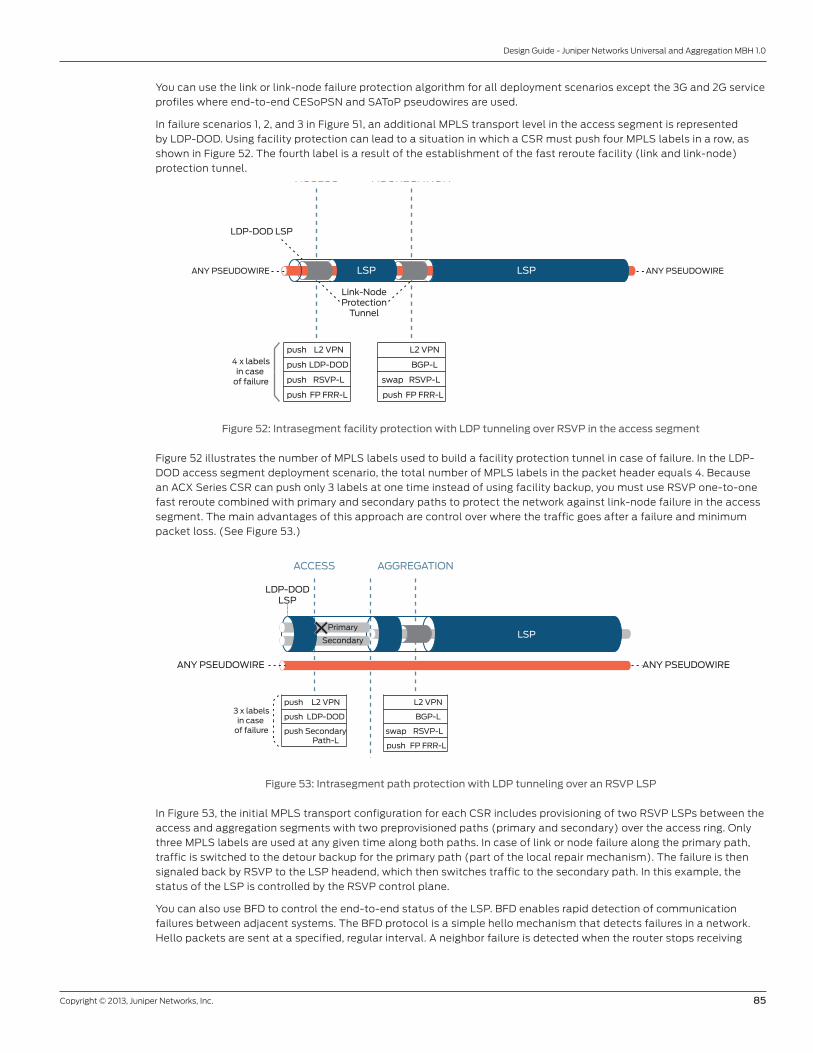
Copyright © 2013, Juniper Networks, Inc. 85
Design Guide - Juniper Networks Universal and Aggregation MBH 1.0
You can use the link or link-node failure protection algorithm for all deployment scenarios except the 3G and 2G service
profiles where end-to-end CESoPSN and SAToP pseudowires are used.
In failure scenarios 1, 2, and 3 in Figure 51, an additional MPLS transport level in the access segment is represented
by LDP-DOD. Using facility protection can lead to a situation in which a CSR must push four MPLS labels in a row, as
shown in Figure 52. The fourth label is a result of the establishment of the fast reroute facility (link and link-node)
protection tunnel.
4 x labelsin case
of failure
BGP-L
L2 VPN
swap RSVP-L
push FP FRR-L
LDP-DOD
L2 VPN
push RSVP-L
push
push
push
FP FRR-L
ACCESS AGGREGATION
Link-NodeProtection
Tunnel
LDP-DOD LSP
ANY PSEUDOWIRELSPLSPANY PSEUDOWIRE
Figure 52: Intrasegment facility protection with LDP tunneling over RSVP in the access segment
Figure 52 illustrates the number of MPLS labels used to build a facility protection tunnel in case of failure. In the LDP-
DOD access segment deployment scenario, the total number of MPLS labels in the packet header equals 4. Because
an ACX Series CSR can push only 3 labels at one time instead of using facility backup, you must use RSVP one-to-one
fast reroute combined with primary and secondary paths to protect the network against link-node failure in the access
segment. The main advantages of this approach are control over where the traffic goes after a failure and minimum
packet loss. (See Figure 53.)
ACCESS AGGREGATION
LDP-DODLSP
BGP-L
L2 VPN
swap RSVP-L
push FP FRR-L
LDP-DOD
L2 VPN
push SecondaryPath-L
push
push
Secondary
PrimaryLSP
ANY PSEUDOWIRE
3 x labelsin case
of failure
ANY PSEUDOWIRE
Figure 53: Intrasegment path protection with LDP tunneling over an RSVP LSP
In Figure 53, the initial MPLS transport configuration for each CSR includes provisioning of two RSVP LSPs between the
access and aggregation segments with two preprovisioned paths (primary and secondary) over the access ring. Only
three MPLS labels are used at any given time along both paths. In case of link or node failure along the primary path,
traffic is switched to the detour backup for the primary path (part of the local repair mechanism). The failure is then
signaled back by RSVP to the LSP headend, which then switches traffic to the secondary path. In this example, the
status of the LSP is controlled by the RSVP control plane.
You can also use BFD to control the end-to-end status of the LSP. BFD enables rapid detection of communication
failures between adjacent systems. The BFD protocol is a simple hello mechanism that detects failures in a network.
Hello packets are sent at a specified, regular interval. A neighbor failure is detected when the router stops receiving

86 Copyright © 2013, Juniper Networks, Inc.
Design Guide - Juniper Networks Universal and Aggregation MBH 1.0
a reply after a specified interval. BFD works with a wide variety of network environments and topologies. The failure
detection timers for BFD have shorter time limits than the failure detection mechanisms of static routes, providing
faster detection.
Intersegment Transport Protection
Intersegment transport protection covers failure scenarios in which area border routers (ABRs)—AG 1 and AG 3
routers—are involved. This guide predominantly covers AG 1 and AG 3 router failures. These routers play the roles of LSP
headends and LSP stitching points, which define the specific intersegment failure scenarios—7 and 8. To protect the
network against failure scenarios 7 and 8, IGP and BGP convergence is enabled by a few techniques that optimize the
whole convergence process. (See Figure 54.)
AS X AS Y
L2 IS-IS Area 49.0001L1 Is-Is Area 49.000a
eNodeB AG 1.4CSR 1.5
ACCESS SERVICE EDGEPRE-AGGREGATION
AGGREGATION
CORE NETWORKIP/MPLS
AG 1.2
CSR 1.2
AG 2.2
AG 3.1
AG 3.2
PE 1
PE 2CSR 1.4
CSR 1.1 AG 1.3
CSR 1.3
7 8AG 2.1AG 1.1
RSVP LSP RSVP LSP
RSVP LSP
7 8
4G EPC
MME
SGW/PGW
HSS
PCRF
BGP-LU LSPLDP Tunneling
Figure 54: Intersegment transport protection
After notification of a failure event (for example, AG 1.1 is down), devices on the access segment must process the
information and calculate an alternate path. For link state protocols such as IS-IS and OSPF, this means running a
new shortest-path-first (SPF) calculation. For BGP, it means a new labeled path calculation based on criteria such as
weights, local preferences, AS path, and so on.
The SPF calculation finds a new labeled path; the router updates its FIB with the next hop for all affected prefixes. FIB
update is a vendor-specific implementation and can be optimized to cut a significant amount of convergence time.
Juniper Networks implements hierarchical FIB and prefix independent convergence to decrease FIB update time to 10 ms.
Moreover, some decisions about the IGP and BGP design help keep the size of the FIB and RIB tables on the CSRs as
small as possible, which allows the exclusion of unnecessary control plane processor time usage, in conjunction with
BFD to control IGP and BGP sessions. The IGP and BGP design leads to a deterministic and rather small convergence
period, which is in accordance with MBH resiliency requirements for most use cases.
You can use inter-area and inter-AS RSVP traffic engineering but that is complex and not scalable, so we do not
recommend it.
End-to-End Protection
End-to-end protection provides network resiliency against any failure in the entire path from the access node to the
provider service edge router. When you run intersegment and intrasegment protection for the transport MPLS LSP, you
provide faster recovery in scenarios where an end-to-end LSP is used—SAToP and CESoPSN for the 2G service profile,
and an ATM pseudowire (PW3) for the 3G service profile.

Copyright © 2013, Juniper Networks, Inc. 87
Design Guide - Juniper Networks Universal and Aggregation MBH 1.0
In this guide, three deployment scenarios (end-to-end Layer 3 VPN, Layer 2 VPN to Layer 3 VPN termination, and
H-VPLS) do not include end-to-end LSP transport. These scenarios use stitching at the MPLS service level, which
requires some service level intelligence to redirect the traffic to a secondary stitching point in case of primary stitching
point failure.
The following deployment scenarios use protection at the service level:
• End-to-End Layer 3 VPN
• Layer 2 VPN to Layer 3 VPN Termination
• End-to-End Hierarchical VPLS
Layer 3 VPN End-to-End Protection for 4G LTE Profile
An essential aspect of the end-to-end Layer 3 VPN scenario is the U-turn VRF, which is located at preaggregation
nodes and serves for better scalability of the solution in the access level in various topologies. Each access region is
dual-homed to two AG 1 routers. Both Router AG 1.1 and Router AG 1.2 participate in the U-turn VRF and represent a
primary and secondary stitching point at the Layer 3 VPN service level. (See Figure 55.)
U-turnL3 VRF
L3 VPNL3 VPN
AS X AS Y
L2 IS-IS Area 49.0001L1 Is-Is Area 49.000a
eNodeB AG 1.4CSR 1.5
ACCESS SERVICE EDGEPRE-AGGREGATION
AGGREGATION
CORE NETWORKIP/MPLS
AG 1.2
CSR 1.2
AG 2.2
AG 3.1
AG 3.2
PE 1
PE 2CSR 1.4
CSR 1.1 AG 1.3
CSR 1.3
9
9
AG 2.1AG 1.1
4G EPC
MME
SGW/PGW
HSS
PCRF
Figure 55: End-to-end protection for end-to-end Layer 3 VPN
Figure 55 illustrates a failure at Router AG 1.1. Restoration of the failure in the access segment depends on the IGP and
MP-IBGP convergence time, whereas end-to-end restoration between the AG 1.2 router and the AG 3 routers is based
on BGP-LU and MP-EBGP convergence.
Pseudowire Redundancy for the HSPA Service Profile (Layer 3 VPN)
Layer 2 VPN to Layer 3 VPN termination scenarios use active and backup pseudowires for the stitching point (AG 1
routers) failure protection at the service level in the access segment. Pseudowires are terminated on logical tunnel
interfaces, which in turn are placed into Layer 3 VPNs on both the AG 1.1 and AG 1.2 routers. (See Figure 56.)

88 Copyright © 2013, Juniper Networks, Inc.
Design Guide - Juniper Networks Universal and Aggregation MBH 1.0
U-turnL3 VRF
VRRP Virtual IP andMAC Address
L3 VPN
Active PseudowireBackup Pseudowire
L2 VPN
AS X AS Y
L2 IS-IS Area 49.0001L1 Is-Is Area 49.000a
NodeB AG 1.4CSR 1.5
ACCESS SERVICE EDGEPRE-AGGREGATION
AGGREGATION
CORE NETWORKIP/MPLS
AG 1.2
CSR 1.2
AG 2.2
AG 3.1
AG 3.2
PE 1
PE 2CSR 1.4
CSR 1.1 AG 1.3
CSR 1.3
10
10
AG 2.1AG 1.1
RNC
3G
Figure 56: End-to-end protection for Layer 2 VPN to Layer 3 VPN termination scenarios
In Figure 56, to ensure that the system maintains a consistent end-to-end traffic forwarding path during a failure of
Router AG 1.1 or Router AG 1.2, we use the following configuration:
1. Hot-standby mode for the backup pseudowire is switched off, as shown in Figure 57. With this mode, the area border router (ABR) follows the status of the active and backup pseudowire according to the status of the logical tunnel interface (up or down), so that only one ABR is announcing VRF routes to connected CSR prefixes at any given time.
2. Logical tunnel interfaces on both Router AG 1.1 and Router AG 1.2 are configured with VRRP groups with the same virtual IP address. Thus both AG 1 routers use the same virtual MAC address to forward traffic from and to NodeB. In a steady situation in the access segment, traffic from NodeB to Router AG 1.1 and Router AG 1.2 is forwarded to a destination MAC address that is the same for AG 1.1 and AG 1.2 . Therefore, if one of the AG 1 routers goes down, the CSR with pseudowire redundancy configured automatically forwards traffic to the other AG 1 router. Maintaining the same VRRP MAC address for both AG 1 routers avoids significant traffic loss from NodeB to the RNC in case of a failure at either of the AG 1 routers. Note that Figure 56 illustrates a failure at Router AG 1.1.

Copyright © 2013, Juniper Networks, Inc. 89
Design Guide - Juniper Networks Universal and Aggregation MBH 1.0
Iub IP
Iub IPIub IP
NodeB
RNC
3GACCESS PRE-AGGREGATION
AGGREGATION
AG 1.2
CSR 1.n
AG 1.1 AG 3.1
Logical Tunnel (lt) Interface with VRRP Virtual IP
AG 3.2
MP-EBGP
L3 VPNL2 VPN
Tra�c FlowConnection at the Service Level
Active PseudowireBackup Pseudowire (not in hot standby)
MP-EBGP
Figure 57: Maintaining traffic path consistency for Layer 2 VPN termination to Layer 3 VPN
In the access segment, the failure scenarios are worked out by the pseudowire control plane, which in this case installs
a backup pseudowire into the FIB only after PE failure detection. In Figure 57, restoration at both ends is consistent
between pseudowire redundancy and MP-EBGP. The blue arrow that extends from NodeB to the RNC represents a
consistent flow of traffic. We configured the CSR with a Layer 2 VPN pseudowire (red circle and red dashed line); the
AG 1 routers with a Layer 2 VPN and Layer 3 VPN (red circle within a green circle); and the AG 3 routers with only a
Layer 3 VPN (green circle). When Router AG 1.1 goes down, the backup pseudowire comes up. Then the logical tunnel
interfaces on AG 1.2 come up, and AG 1.2 announces itself as an active node for the Layer 3 VPN. In this situation, both
MP-EBGP and the configured backup pseudowire determine that AG 1.1 is down and traffic is forwarded across the
Layer 3 VPN.
End-to-end restoration between Router AG 1.2 and the AG 3 routers is based on BGP-LU and MP-EBGP convergence. It
is possible that the HSPA RNC is located closer to NodeB than to the AG 2 routers, which can play the role of the edge
service PE to interconnect the MBH network to the RNC. In this case, restoration time for traffic forwarding between the
AG 1 routers and the AG 2 routers relies on MP-IBGP and the IGP protocols.
Pseudowire Redundancy for the HSPA Service (H-VPLS)
In the access segments, Layer 2 VPN to VPLS termination (or H-VPLS) scenarios use active and backup pseudowires
for stitching-point (Router AG 1.1 and Router AG 1.2) failure protection at the service level. Pseudowires are terminated
on the label-switched interfaces (LSIs), which in turn are placed into a VPLS on both Router AG 1.1 and Router AG 1.2.
The LSI interface does not require any configuration. Instead of configuring the LSI, we configure a mesh group in a
routing instance. (See Figure 58.)

90 Copyright © 2013, Juniper Networks, Inc.
Design Guide - Juniper Networks Universal and Aggregation MBH 1.0
VPLSHub
LSIInterface
VPLSL2 VPN
Active PseudowireBackup Pseudowire
RNC
3G
AS X AS Y
L2 IS-IS Area 49.0001L1 Is-Is Area 49.000a
NodeB AG 1.4CSR 1.5
ACCESS SERVICE EDGEPRE-AGGREGATION
AGGREGATION
CORE NETWORKIP/MPLS
AG 1.2
CSR 1.2
AG 2.2
AG 3.1
AG 3.2
PE 1
PE 2CSR 1.4
CSR 1.1 AG 1.3
CSR 1.3
11
11
AG 2.1AG 1.1
Figure 58: End-to-end protection for HSPA service profile (H-VPLS deployment scenario)
In Figure 58, hot-standby mode for active and backup pseudowires in conjunction with the regular MAC learning
process allows consistent and rapid service restoration in case of failure on the AG 1 routers.
The following event sequence shows the restoration process after Router AG 1.1 fails:
1. Router AG 1.1 goes down.
2. Traffic flows from NodeB to the RNC undergo the following process:
a. The CSR detects that the active pseudowire is down and switches traffic forwarding to the presignaled backup pseudowire.
b. Router AG 1.2 receives a packet from the CSR, learns the NodeB MAC address, puts the MAC address into its MAC learning table, and broadcasts the packet to VPLS neighbors as an unknown unicast packet.
c. The remote provider edge routers (PE 1 and PE 2) receive the packet from Router AG 1.2 and relearn the MAC address of NodeB; then the PE routers map the NodeB MAC address to Router AG 1.2 in their MAC learning tables.
3. Traffic flows from the RNC to NodeB undergo the following process:
a. The RNC sends the packet to the NodeB MAC address.
b. Traffic from the RNC goes to one of the remote provider edge routers, such as PE 1.
c. Router PE 1 forwards traffic to Router AG 1.2 based on updated records in the MAC learning table.
d. Router AG 1.2 receives packets, learns the RNC MAC address, puts it into the MAC learning table, and forwards packets to the CSR over the secondary pseudowire.
4. A consistent traffic path is installed in both directions.

Copyright © 2013, Juniper Networks, Inc. 91
Design Guide - Juniper Networks Universal and Aggregation MBH 1.0
Network Management You need to consider two tasks when designing network management for the MBH network. The first task is to provide
transport services for the MBH. The second task is to build a complete set of network management solutions that
manage and control the MBH network itself. According to fault, configuration, accounting, performance, and security
(FCAPS) as defined by the ISO network management model or some pieces of it, the ideal solution is to integrate these
two tasks into one management solution.
Providing Transport Services for Network Management To separate customer and provider traffic, the various nodes in the network can be connected to the management
entity by an out-of-band network, an in-band network using VLAN technology, and an MPLS pseudowire. If the MPLS
pseudowire or VLAN approach is not scalable, then VRF-Lite-based connectivity can also be used.
We recommend that you use a separate management Layer 3 VRF routing instance type that scales well and provides
separation between the customer and the provider management planes. From the network service point of view, any
of these techniques—end-to-end Layer 3 VPN, pseudowire termination to Layer 3 VPN, and pseudowire termination to
VPLS—can be used for the management planes and in most cases depends on customer preferences.
MBH Network Management System Provisioning is a difficult topic to address in the service provider network because each customer has unique challenges
and requirements. Some service providers use a network management system (NMS) for complete network discovery
and provisioning, and others use a hybrid model of control plane and NMS.
Within the proposed solution, the Junos Space NMS can serve as an ideal candidate for the MBH network NMS. The
Junos OS by itself also provides a comprehensive user command-line interface (CLI) to achieve network management.
The biggest advantage that the Junos OS brings is that all platforms in the access and aggregation network have a
common uniform CLI for static provisioning, which makes maintaining the network straightforward.
The Junos Space comprehensive FCAPS toolkit simplifies network and service deployment and management tasks.
The Network Activate application provisions VPNs up to 10 times faster than manual configuration. The Service Now
application reduces mean-time-to-resolution (MTTR) up to 30 times by transmitting the details of the network to
a Juniper Networks support site even before the customer calls. Route Insight provides remarkable visibility into the
network and also allows the simulation of network changes before they are committed.
Below is an outline of the Junos Space functional role within the MBH solution:
• IP/MPLS transport provisioning (Transport Activate)
• Service provisioning (Network Activate)
• CoS provisioning (CoS design)
• Synchronization design
• OAM insight
• Monitoring
• Fault management
• Zero touch deployment
• API to easily integrate into existing NMS or operations and business support systems (OSS/BSS) deployments
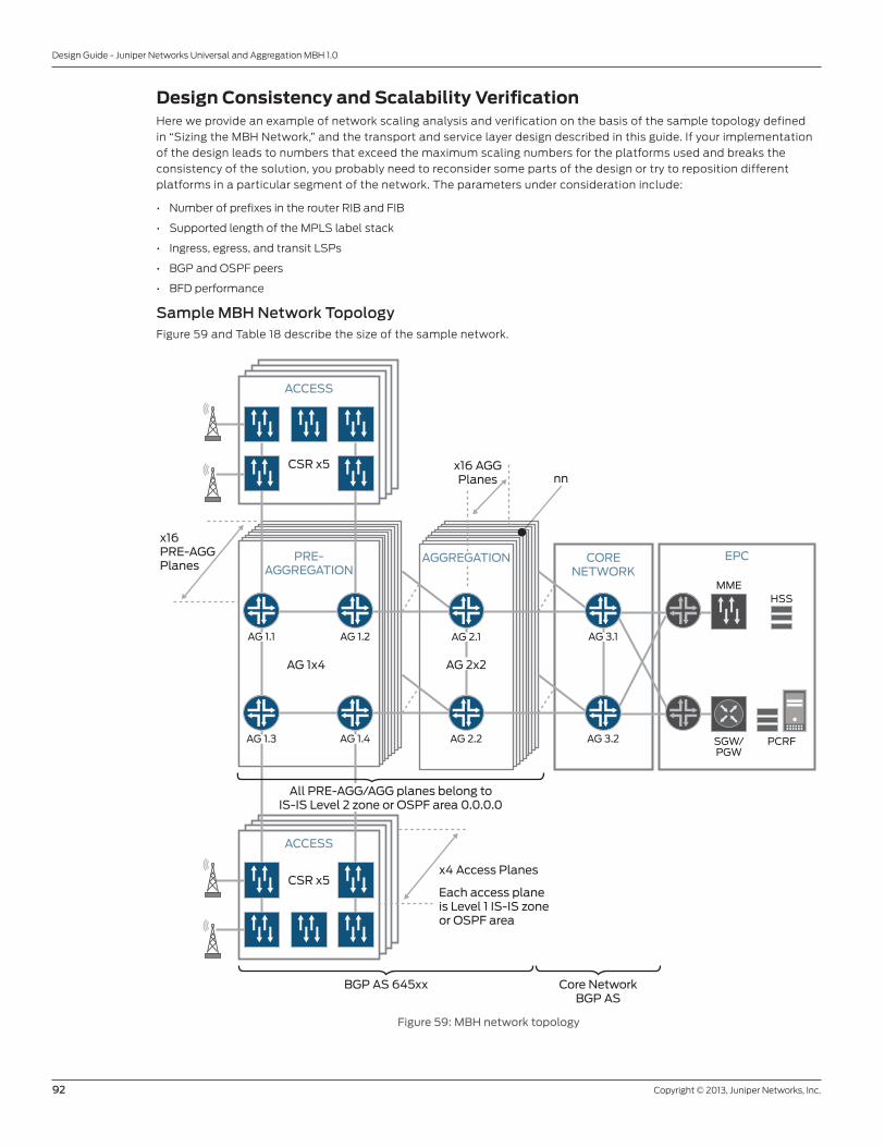
92 Copyright © 2013, Juniper Networks, Inc.
Design Guide - Juniper Networks Universal and Aggregation MBH 1.0
Design Consistency and Scalability VerificationHere we provide an example of network scaling analysis and verification on the basis of the sample topology defined
in “Sizing the MBH Network,” and the transport and service layer design described in this guide. If your implementation
of the design leads to numbers that exceed the maximum scaling numbers for the platforms used and breaks the
consistency of the solution, you probably need to reconsider some parts of the design or try to reposition different
platforms in a particular segment of the network. The parameters under consideration include:
• Number of prefixes in the router RIB and FIB
• Supported length of the MPLS label stack
• Ingress, egress, and transit LSPs
• BGP and OSPF peers
• BFD performance
Sample MBH Network TopologyFigure 59 and Table 18 describe the size of the sample network.
PRE-AGGREGATION
ACCESS
CORENETWORK
x4 Access Planes
AG 1x4
CSR x5
CSR x5
ACCESS
AG 3.1
AG 3.2AG 2.2
AG 2.1AG 1.1 AG 1.2
AG 1.3 AG 1.4
AGGREGATION
AG 2x2
CSR x5
MME
SGW/PGW
HSS
PCRF
EPC
nn
Each access planeis Level 1 IS-IS zoneor OSPF area
x16PRE-AGGPlanes
x16 AGGPlanes
All PRE-AGG/AGG planes belong toIS-IS Level 2 zone or OSPF area 0.0.0.0
BGP AS 645xx Core NetworkBGP AS
Figure 59: MBH network topology

Copyright © 2013, Juniper Networks, Inc. 93
Design Guide - Juniper Networks Universal and Aggregation MBH 1.0
Table 18: Sample Network Segment Size
Number of Nodes AG 3 Nodes AG 2 Nodes AG 1 Nodes ANs Nodes
Per regional network 2 32 1,024 10,240
Per AG 3 router - 32 1,024 10,240
Per AG 2 ring - 2 64 640
Per AG 1 ring - - 4 40
AssumptionsBefore proceeding, we must make some assumptions about the service profiles that are in the topology.
1. All four service profiles—4G LTE, HSPA, 3G, and 2G—are configured in the network, and each cell site router (CSR) connects to at least one radio access network (RAN) cell of each service generation. Table 19 summarizes this assumption. For example:
• X2, S1-U, and S1-MME connectivity is provided by three separate end-to-end Layer 3 VPNs.
• eNodeBs are connected to CSRs by Gigabit Ethernet.
• VLAN tagging is used for service separation on the link.
• EPC is connected to Router AG 3.1 and Router AG 3.2.
2. An Ethernet-based EPC and RNC are connected to provider service edge routers and legacy-based controllers connected to Router AG 2.1 and Router AG 2.2, leading to 16 different BSCs (TDM) and RNCs (ATM), respectively. (See Table 19.)
Table 19: Sample Network Services and Service Locations
Service Profile RAN Type Port/VLAN Type of Mobile Network interface
Service Deployment Scenario
EPC/RNC/BSC Router Location
4G LTE eNodeB ge-0/0/1.1 vlan-id 1
X2 End-to-end Layer 3 VPN
-
eNodeB ge-0/0/1.2 vlan-id 2
S1 user plane End-to-end Layer 3 VPN
AG 3.1/AG 3.2
eNodeB ge-0/0/1.3 vlan-id 3
S1-MME End-to-end Layer 3 VPN
AG 3.1/AG 3.2
HSPA NodeB ge-0/0/2.5 vlan-id 5
Iub over IP Layer 2 VPN to Layer 3 VPN termination
AG 3.1/AG 3.2
HSPA NodeB ge-0/0/3.0 Iub over Ethernet H-VPLS AG 3.1/AG 3.2
3G NodeB at-0/0/16 Iub over ATM ATM pseudowire (PW3)
AG 2.1.n/AG 2.2.nn=1…16
2G BTS e1-0/0/1 Abis over TDM SAToP AG 2.1.n/AG 2.2.nn=1…16
- eNodeB ge-0/0/1.4vlan-id 4
Mobile network management
End-to-end Layer 3 VPN management
AG 3.1/AG 3.2
3. Any-to-any Layer 3 connectivity between eNodeBs is required:
• Within the 4G LTE service profile for X2 Layer 3 VPN only
• Between eNodeBs that belong to any three adjacent AG 2 segments.
4. IP prefix of /30 is used on the interface between eNodeB and the CSR.
5. IS-IS is chosen for interior gateway protocol (IGP) routing.
6. The design of IGP regions and MPLS transport is described in the following topics:
• End-to-End IP/MPLS Transport Design
• Intradomain LSP Signaling
• Interdomain LSP Signaling with BGP-labeled unicast
7. The configuration of all AG 1 routers with a U-turn VRF is described in the following topics:
• End-to-End Layer 3 VPN Design
• Layer 2 VPN to Layer 3 VPN Termination Scenario

94 Copyright © 2013, Juniper Networks, Inc.
Design Guide - Juniper Networks Universal and Aggregation MBH 1.0
8. The configuration of all service profiles is described in the following topics:
• End-to-End Layer 3 VPN Design
• Layer 2 VPN to Layer 3 VPN Termination Scenario
• Hierarchical VPLS for Iub over Ethernet
• MPLS Service Design for the 3G Service Profile
• MPLS Service Design for the 2G Service Profile
Cell Site Router Scaling Analysis
RIB and FIB Scaling
In Juniper Networks Solution Portfolio, ACX Series routers are situated in the access segment. Being a cost-optimized
platform, ACX Series routers have less scaling than MX Series routers. In addition, the ACX Series routers have specific
restrictions that you must take into account and that require attention to scaling.
The size of the routing information base (RIB) and the forwarding information base (FIB) is an essential parameter of
any routing platform. In this guide, we pay attention to decreasing the amount of routing intelligence needed in CSRs.
Table 20 summarizes the number of records in the RIB and the FIB for CSRs, and is in line with the design and services
presented in this guide.
Table 20: Scaling Analysis and Verification for the CSR FIB
Node Protocol IP Prefixes RIB FIB Notes
CSR IGP (IS-IS) routes
Loopback/32 5*4 + 2 RIB*2 = 44 Multiplier four (*4) stands for four IGP access regions. (See the topic “Intradomain LSP Signaling” and Figure 59.) Multiplier two (*2) stands for two paths in a ring.
Infrastructure/30 7*4 RIB*2 = 28
Static routes to AG 1 routers 2 2
Directly connected
MP-BGP VRF prefixes/30, plus lo0.1/32, plus summarized routes from AG 1 routers
1 + 1 + 1 RIB*2 = 6 Layer 3 VPN X2
MP-BGP 1 + 1 + 1 RIB*2 = 6 Layer 3 VPN S1 user plane
MP-BGP 1 + 1 + 1 RIB*2 = 6 Layer 3 VPN S1-MME
MP-BGP 1 + 1 + 1 RIB*2 = 6 Layer 3 VPN management
Total routes installed in the FIB 98
MPLS Label FIB (L-FIB) Scaling
ACX Series routers have platform-specific limitations for the MPLS forwarding plane in relation to the number of
MPLS labels that can be programmed into the MPLS L-FIB of the network processor. The following three types of
labels are counted:
1. Advertised labels to establish the egress LSP (out labels)
2. Received labels to establish the ingress LSP (in label bundled with the next hop)
3. Service labels for the Layer 3 VPN, Layer 2 VPN, ATM, and TDM pseudowires, and for VPLS
Table 21 contains data for the transport of ingress and egress LSPs. Table 22 shows the number of service labels on
a CSR.
Table 21: Cell Site Router Scaling Analysis for the L-FIB
Node Protocol LSP L-FIBOut/In
Notes
CSR RSVP CSR to Router AG 1.1 and Router AG 1.2
4/4 Take into account the primary and secondary paths configured for each LSP.
Transit LSPs 16/16
BGP-LU N/A
LDP-DOD over RSVP
CSR to Router AG 2.1 and Router AG 2.2
1*2/2*2 Tunnel used by ATM and TDM pseudowires. Multiplier two (*2) stands for CSRs dual homed to Router AG 1.1 and Router AG 1.2.
Transit 0/0
Total routes installed in the FIB

Copyright © 2013, Juniper Networks, Inc. 95
Design Guide - Juniper Networks Universal and Aggregation MBH 1.0
Table 22: Cell Site Router Scaling Analysis for Service Labels
Node Protocol MPLS VPN Service Labels Out/In
Service Profile
Out/In Service Profile
Pseudowires from CSRs to Router AG 1.1 and Router AG 1.2
2/2 Layer 2 VPN to Layer 3 VPN for HSPA
T-LDP Pseudowires from CSRs to Router AG 1.1 and Router AG 1.2
2/2 Layer 2 VPN to VPLS for HSPA
T-LDP Pseudowires from CSRs to Router AG 1.1 and Router AG 1.2
2/2 ATM pseudowire
T-LDP Pseudowires from CSRs to Router AG 1.1 and Router AG 1.2
2/2 TDM pseudowire
MP-BGP Layer 3 VPN X2 2/2
MP-BGP Layer 3 VPN S1 user plane 2/2 Layer 3 VPN S1 user plane
MP-BGP Layer 3 VPN S1-MME 2/2 Layer 3 VPN S1-MME
MP-BGP Layer 3 VPN management 2/2 Layer 3 VPN management
Total number of service labels 16/16
Another important parameter, with regard to MPLS is the size of the label stack in the MPLS packet header. For ACX
Series routers, the maximum number of labels that can be simultaneously popped, pushed, or swapped is three labels.
This subject is discussed in detail in the topic “Intrasegment Transport Protection.”
CSR Scaling Analysis
Table 23 summarizes values for the most critical parameters of CSRs that might require attention during the design,
planning, and verification phases of the solution.
Table 23: Cell Site Router Scaling Analysis
Parameter Description Valueby Design
ACX Series Maximum Value(Junos OS 12.3)
IPv4 entries per router 98 20,000
• IPv4 entries 74 20,000
• IPv4 entries per VRF instance 24 20,000
Network routers per IS-IS area 7 250
IS-IS adjacencies per router 2 250
Network routers per OSPF area 7 250
OSPF adjacencies per router 2 250
VRF table per router 4 64
BGP adjacencies per router 2 256
LDP adjacencies per router 2 100
RSVP adjacencies per router 2 2,000
Total number of transport labels 46 3,000
Maximum depth of the label stack 3 3
Total service MPLS labels: 32 1,000
• VRF table per router 8 64
• CESoPSN pseudowire (PWE3) 2 496
• ATM pseudowire (PWE3) 2 1,000
• Ethernet pseudowire (PWE3) 4 1,000
Total number of BFD sessions: 30 @ 10 ms 256 @ 100 ms
• BFD for IGP 2 @ 10 ms
• BFD for RSVP 4 @ 100 ms
Total number of slaves for an IEEE 1588v2 boundary clock 512 @ 128 mps 512 @ 128 mps

96 Copyright © 2013, Juniper Networks, Inc.
Design Guide - Juniper Networks Universal and Aggregation MBH 1.0
AG 1 Router Scaling Analysis
RIB and FIB Scaling
The AG 1 routers are the aggregation routers that connect the access segment to the aggregation segment. The
MX80-P router is qualified in this position. Table 24 summarizes the number of records in the RIB and the FIB for AG 1
routers, and is in line with the design and services presented in this guide.
Table 24: AG 1 Router Scaling Analysis for the FIB
Node Protocol IP Prefixes RIB FIB Notes
AG 1 IGP (IS-IS) routes
Loopback/32 2 + 64 + 640 = 706 RIB*2 = 1412 Multiplier two (*2) stands for two paths in a ring. Multiplier five (*5) stands for five paths in a ring.
Infrastructure/30 16*5 = 80 RIB*2 = 160
Static routes to AG 1 routers
5 5
MP-BGP CSR VRF routes/30, plus CSR lo0.1/32, plus local lo0.1/32
3*640+3*640+3*64
RIB*2 = 8,064 Layer 3 VPN X2.Multiplier two (*2) stands for BGP multipath.Multiplier three (*3) stands for three neighboring areas for X2 connectivity.
MB-BGP CSR VRF routes/30, plus CSR lo0.1/32, plus local lo0.1/32, plus AG 3 VRF routes/24, plus AG 3 lo0.1/32
20+20+1+5+2
RIB*2 = 94 Layer 3 VPN S1 user plane
MB-BGP Same as for Layer 3 VPN S1
47 RIB*2 = 94 Layer 3 VPN S1-MME
47 RIB*2 = 94 Layer 3 VPN HSPA
47 RIB*2 = 94 Layer 3 VPN management
Total IGP routes installed in the FIB 1,577
Total VRF routes 8,440
MPLS Label FIB (L-FIB) Scaling
ACX Series routers have platform-specific limitations for the MPLS forwarding plane in relation to the number of MPLS
labels that can be programmed into the MPLS label-forwarding information base (L-FIB) of the network processor. The
following three types of labels are counted:
1. Advertised labels to establish the egress LSP (out labels)
2. Received labels to establish the ingress LSP (in label bundled with the next hop).
3. Service labels for the Layer 3 VPN, Layer 2 VPN, ATM, and TDM pseudowires, and for VPLS
Table 25 contains data for the transport of ingress and egress LSPs. Table 26 shows the number of service labels on an
AG 1 router.
Table 25: AG 1 Router Scaling Analysis for the L-FIB
Node Protocol LSP L-FIBOut/In
Notes
AG 1 RSVP AG 1 routers to AG 1 and AG 2 routers
65/65 Full mesh LSP in the IS-IS Level 2 region.
Transit AG 1 routers to AG 1 routers and AG 2 routers
(4 - 1)*65/135
AG 1 routers to CSRs 40/40 Hub-and-spoke LSP within the IS-IS Level 1 region.
Transit AG 1 routers to CSRs
40/40
BGP-LU Announced AG 1 and CSRs loopback addresses
21/0
Received loopback addresses from AG 1 routers, AG 2 routers, and AG 3 routers1
0/64*2*2 The first multiplier two (*2) is used to provide X2 connectivity to two adjacent AG 2 areas. The second multiplier (*2) stands for dual-homing peering to Router AG 2.1 and Router AG 2.2.
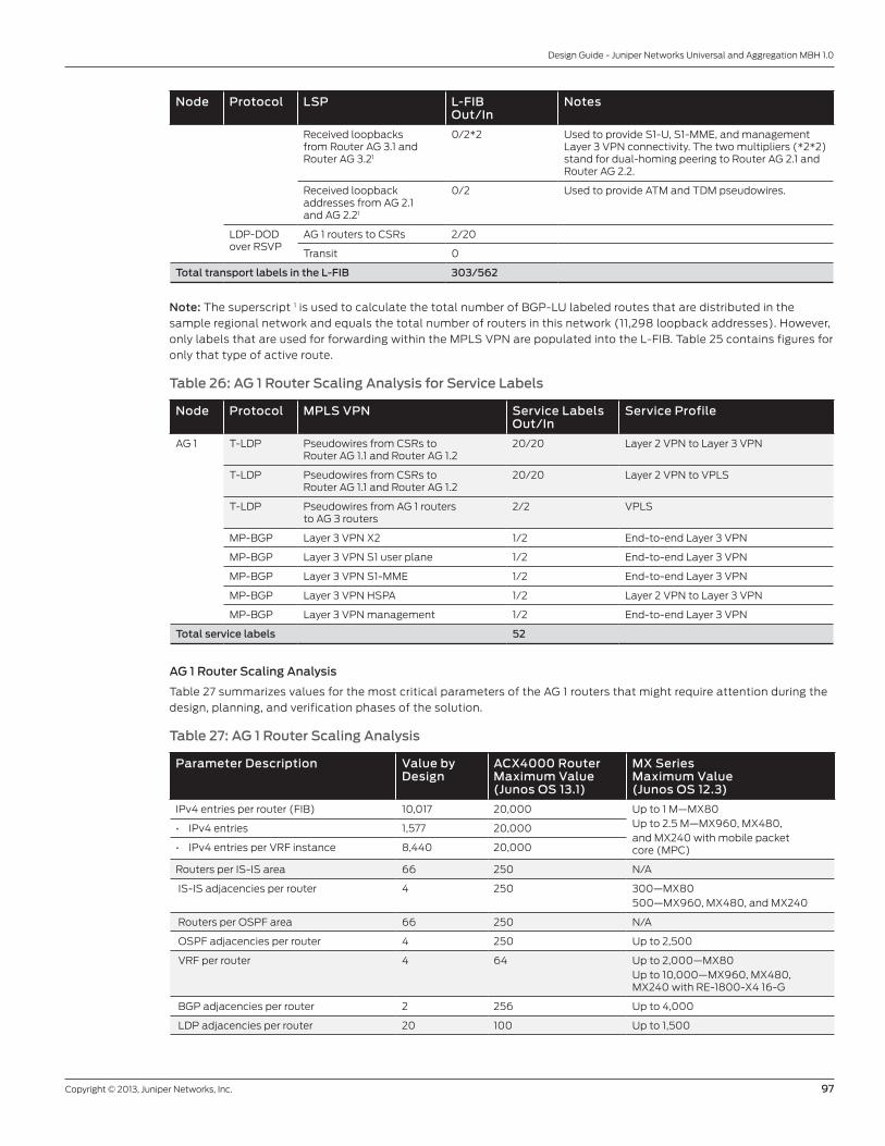
Copyright © 2013, Juniper Networks, Inc. 97
Design Guide - Juniper Networks Universal and Aggregation MBH 1.0
Node Protocol LSP L-FIBOut/In
Notes
Received loopbacks from Router AG 3.1 and Router AG 3.21
0/2*2 Used to provide S1-U, S1-MME, and management Layer 3 VPN connectivity. The two multipliers (*2*2) stand for dual-homing peering to Router AG 2.1 and Router AG 2.2.
Received loopback addresses from AG 2.1 and AG 2.21
0/2 Used to provide ATM and TDM pseudowires.
LDP-DOD over RSVP
AG 1 routers to CSRs 2/20
Transit 0
Total transport labels in the L-FIB 303/562
Note: The superscript 1 is used to calculate the total number of BGP-LU labeled routes that are distributed in the
sample regional network and equals the total number of routers in this network (11,298 loopback addresses). However,
only labels that are used for forwarding within the MPLS VPN are populated into the L-FIB. Table 25 contains figures for
only that type of active route.
Table 26: AG 1 Router Scaling Analysis for Service Labels
Node Protocol MPLS VPN Service LabelsOut/In
Service Profile
AG 1 T-LDP Pseudowires from CSRs to Router AG 1.1 and Router AG 1.2
20/20 Layer 2 VPN to Layer 3 VPN
T-LDP Pseudowires from CSRs to Router AG 1.1 and Router AG 1.2
20/20 Layer 2 VPN to VPLS
T-LDP Pseudowires from AG 1 routers to AG 3 routers
2/2 VPLS
MP-BGP Layer 3 VPN X2 1/2 End-to-end Layer 3 VPN
MP-BGP Layer 3 VPN S1 user plane 1/2 End-to-end Layer 3 VPN
MP-BGP Layer 3 VPN S1-MME 1/2 End-to-end Layer 3 VPN
MP-BGP Layer 3 VPN HSPA 1/2 Layer 2 VPN to Layer 3 VPN
MP-BGP Layer 3 VPN management 1/2 End-to-end Layer 3 VPN
Total service labels 52
AG 1 Router Scaling Analysis
Table 27 summarizes values for the most critical parameters of the AG 1 routers that might require attention during the
design, planning, and verification phases of the solution.
Table 27: AG 1 Router Scaling Analysis
Parameter Description Value by Design
ACX4000 Router Maximum Value(Junos OS 13.1)
MX SeriesMaximum Value(Junos OS 12.3)
IPv4 entries per router (FIB) 10,017 20,000 Up to 1 M—MX80Up to 2.5 M—MX960, MX480, and MX240 with mobile packet core (MPC)
• IPv4 entries 1,577 20,000
• IPv4 entries per VRF instance 8,440 20,000
Routers per IS-IS area 66 250 N/A
IS-IS adjacencies per router 4 250 300—MX80500—MX960, MX480, and MX240
Routers per OSPF area 66 250 N/A
OSPF adjacencies per router 4 250 Up to 2,500
VRF per router 4 64 Up to 2,000—MX80Up to 10,000—MX960, MX480, MX240 with RE-1800-X4 16-G
BGP adjacencies per router 2 256 Up to 4,000
LDP adjacencies per router 20 100 Up to 1,500

98 Copyright © 2013, Juniper Networks, Inc.
Design Guide - Juniper Networks Universal and Aggregation MBH 1.0
Parameter Description Value by Design
ACX4000 Router Maximum Value(Junos OS 13.1)
MX SeriesMaximum Value(Junos OS 12.3)
RSVP adjacencies per router 2 2,000 Up to 50,000
Number of transport labels 46 3,000 N/A
Maximum depth of the label stack 3 or 4 3 4
MPLS LSP per router 2,000 Up to 50,000
Total service MPLS labels 16 1,000 N/A
• VRF per router 8 64
• CESoPSN pseudowire (PWE3) 2 496
• ATM pseudowire (PWE3) 2 1,000
• Ethernet pseudowire (PWE3) 4 1,000
Total number of BFD sessions 30 @ 10 ms256 @ 100 ms
• BFD for the IGP 4 @ 10 ms
• BFD for RSVP 172 @ 100 ms
Total number of slaves for an IEEE 1588v2 boundary clock
20 @ 128 mps 512 @ 128 mps 20 @ 128 mps
Note: The maximum values are not guaranteed and depend on various factors, such as the network configuration and
conditions, and should not be taken literally. These values are provided as a comparison to the values required for the
sample solution.
AG 2 Router Scaling Analysis
RIB and FIB Scaling
The AG 2 routers are the aggregation routers that aggregate the AG 1 rings (16 rings with four AG 1 routers per ring) and
connect the aggregation segment to the core segment. MX240 and MX480 platforms are qualified in this position.
Table 28 summarizes the number of records in the RIB and the FIB for AG 2 routers, and is in line with the design and
services presented in this guide.
Table 28: AG 2 Router Scaling Analysis for the FIB
Node Protocol IP Prefixes RIB FIB Notes
AG 2 IGP (IS-IS) routes
Loopback/32 2 + 64 + 640 = 706 RIB*2 = 1,412 Multiplier two (*2) stands for two paths in a ringInfrastructure/30 80 RIB*2 = 160
Total routes installed in the FIB 1,572
MPLS Label FIB Scaling
Table 29 contains data for the transport of ingress and egress LSPs. Table 30 shows the number of service labels on
the AG 2 routers.
Table 29: AG 2 Router Scaling Analysis for the L-FIB
Node Protocol MPLS Labels L-FIBOut/In
Notes
AG 2 RSVP label Advertised/received 65/65 Full mesh in the IS-IS Level 2 region. (64* AG 1, 2*AG 2).
Transit 4,096/4,096
BGP-LU Received AG 1 loopback addresses from Router AG 3.1 and Router AG 1.21
0/64*2*2 The first multiplier two (*2) is used to provide X2 connectivity to two adjacent AG 2 areas. The second multiplier (*2) stands for dual-homing peering to Router AG 3.1 and Router AG 3.2.
BGP-LU Received AG 1 loopback addresses from the AG 1 ring1
0/64*2 Used to provide X2 connectivity to two adjacent AG 2 areas. The multiplier (*2) stands for two paths in a ring from the AG 2 routers to the AG 1 routers.

Copyright © 2013, Juniper Networks, Inc. 99
Design Guide - Juniper Networks Universal and Aggregation MBH 1.0
Node Protocol MPLS Labels L-FIBOut/In
Notes
BGP-LU Advertised loopback addresses to the AG 1 ring1
64 + 1/0 Used to provide X2 connectivity to two adjacent AG 2 areas
BGP-LU Advertised loopback addresses to the AG 31 routers
64 + 1/0 Used to provide X2 connectivity
BGP-LU Received AG 3 loopback address from Router AG 3.1 and Router AG 3.31
2/0 Used to provide S1-U, S1-MME, and management Layer 3 VPN connectivity
BGP-LU Received CSR loopback addresses from the AG 1 ring1
2*640 = 1,280/0 Used to provide ATM and TDM pseudowires
Total transport labels in the L-FIB 5,573/4,545
Note: The superscript 1 is used to calculate the total number of BGP-LU labeled routes that are distributed in the
example regional network and equals the total number of loopback addresses in this network (11,298 loopback
addresses). However, only labels for the used routes are populated into the L-FIB. Table 29 contains figures for only
used routes. However, only labels that are used for forwarding within the MPLS VPN are populated into the L-FIB. Table
29 contains figures for only that type of active route.
Table 30: AG 2 Router Scaling Analysis for Service Labels
Node Protocol MPLS VPN Service LabelsOut/In
Service Profiles
AG 2 T-LDP Pseudowires from CSRs to Router AG 2.1 and Router AG 2.2
640/640 ATM pseudowire—PW3
T-LDP Pseudowires from CSRs to Router AG 2.1 and Router AG 2.2
640/640 SAToP
Total service labels 1,280/1,280
AG 3 Router Scaling Analysis
RIB and FIB Scaling
IGP protocols deployed on Router AG 3.1 and Router AG 3.2 are part of the service provider core network, so a
reasonable number of loopback/32 and infrastructure/30 routes must be added to the results in the table below.
Table 31 summarizes the number of records in the RIB and the FIB for AG 3 routers, and is in line with the design and
services presented in this guide.
Table 31: AG 3 Router Scaling Analysis for the FIB
Node Protocol IP Prefixes RIB FIB Notes
AG 3 MP-BGP CSR VRF routes /24, plus CSR lo0.1/32, plus the AG 1 routers lo0.1/32, and the Router AG 3.1 and Router AG 3./2 lo0.1/32
4*10,240+4*10,240+4*640+4*2
RIB*2 = 21,762 Multiplier four (4*) stands for the number of Layer 3 VPNsMultiplier two (*2) stands for BGP multipath
Loopback/32 2 10
IGP Infrastructure/30 8
Total IGP routes installed in the FIB 10+
Total VRF routes 21,762
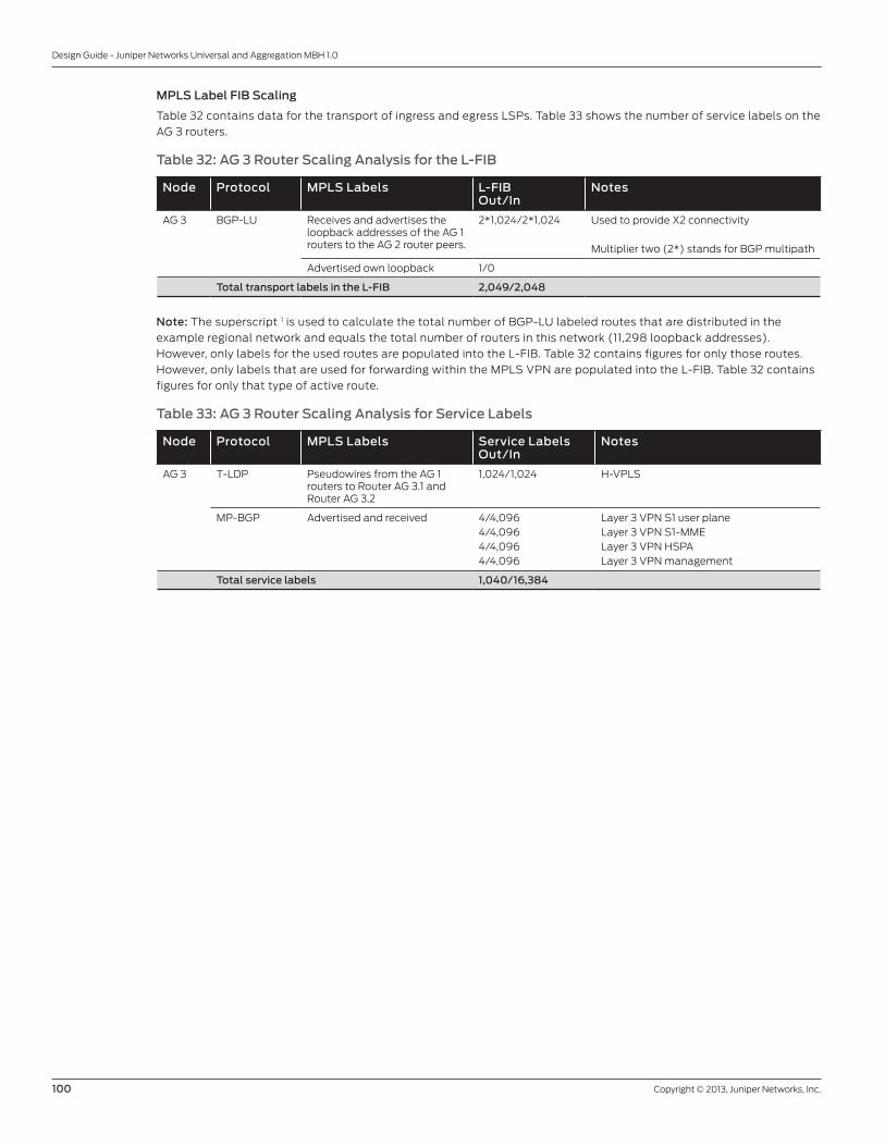
100 Copyright © 2013, Juniper Networks, Inc.
Design Guide - Juniper Networks Universal and Aggregation MBH 1.0
MPLS Label FIB Scaling
Table 32 contains data for the transport of ingress and egress LSPs. Table 33 shows the number of service labels on the
AG 3 routers.
Table 32: AG 3 Router Scaling Analysis for the L-FIB
Node Protocol MPLS Labels L-FIBOut/In
Notes
AG 3 BGP-LU Receives and advertises the loopback addresses of the AG 1 routers to the AG 2 router peers.
2*1,024/2*1,024 Used to provide X2 connectivity
Multiplier two (2*) stands for BGP multipath
Advertised own loopback 1/0
Total transport labels in the L-FIB 2,049/2,048
Note: The superscript 1 is used to calculate the total number of BGP-LU labeled routes that are distributed in the
example regional network and equals the total number of routers in this network (11,298 loopback addresses).
However, only labels for the used routes are populated into the L-FIB. Table 32 contains figures for only those routes.
However, only labels that are used for forwarding within the MPLS VPN are populated into the L-FIB. Table 32 contains
figures for only that type of active route.
Table 33: AG 3 Router Scaling Analysis for Service Labels
Node Protocol MPLS Labels Service LabelsOut/In
Notes
AG 3 T-LDP Pseudowires from the AG 1 routers to Router AG 3.1 and Router AG 3.2
1,024/1,024 H-VPLS
MP-BGP Advertised and received 4/4,0964/4,0964/4,0964/4,096
Layer 3 VPN S1 user planeLayer 3 VPN S1-MMELayer 3 VPN HSPALayer 3 VPN management
Total service labels 1,040/16,384

Copyright © 2013, Juniper Networks, Inc. 101
Design Guide - Juniper Networks Universal and Aggregation MBH 1.0
Part 3: ImplementationThis part of the guide describes how to configure a mobile backhaul (MBH) network based on the various scenarios
presented in Part 2. It focuses on Juniper Networks hardware and software platforms as the building blocks and
contains the following overview topics and sample configurations:
• Recommendations for IGP Region Numbering and Network Addressing
• Network Topology Overview
• Configuring IP and MPLS Transport
• Configuring End-to-End Layer 3 VPN Services
• Configuring Layer 2 VPN to Layer 3 VPN Termination Services
• Configuring a Layer 2 VPN to VPLS Termination Service
• Configuring ATM Pseudowire and SAToP/CESoPSN Services
• Configuring Timing and Synchronization
• Configuring Class of Service
All of the sample configurations use a ring topology and IS-IS as the IGP. The configurations were tested as part of a
complex solution with all the necessary protocols configured simultaneously within the sample network topology and
verified against different failure scenarios.

102 Copyright © 2013, Juniper Networks, Inc.
Design Guide - Juniper Networks Universal and Aggregation MBH 1.0
Recommendations for IGP Region Numbering and Network Addressing These IGP region numbering and network addressing recommendations can easily be adapted to most larger scale
deployments. The recommendations are for network addressing, interior gateway protocol (IGP) regions, and BGP
autonomous system (AS) numbering, and are covered in the following topics:
• Loopback and Infrastructure IP Addressing
• UNI Addressing and Layer 3 VPN Identifier
• Management (fxp0) Interface Addressing
To illustrate the basic principles of designing IGP numbering and network addressing, see the topic “Sizing the MBH
Network” for an example of a large-scale network. (See Figure 60.)
PRE-AGGREGATION
ACCESS
CORENETWORK
x4 Access Planes
AG 1x4
CSR x5
CSR x5
ACCESS
AG 3.1
AG 3.2AG 2.2
AG 2.1AG 1.1 AG 1.2
AG 1.3 AG 1.4
AGGREGATION
AG 2x2
CSR x5
MME
SGW/PGW
HSS
PCRF
EPC
nn
Each access planeis Level 1 IS-IS zoneor OSPF area
x16PRE-AGGPlanes
x16 AGGPlanes
PRE-AGG/AGG planes belong toIS-IS Level 2 zone or OSPF area 0.0.0.0
BGP AS 645xx Core NetworkBGP AS
Figure 60: Regional large-scale MBH network
In Figure 60, we have 16 independent aggregation (AG G) planes defined by 16 pairs of AG 2.1 and AG 2.2 routers. The
access, preaggregation, and aggregation segments correspond to one aggregation (AG G) plane and belong to one
BGP AS 645xx, while the core segment belongs to a different core network AS. You can select the AS number from
the private range of AS numbers that extend from 64,512 through 65,535. We recommend that you reserve a small
subrange of 10-20 AS numbers per regional network.

Copyright © 2013, Juniper Networks, Inc. 103
Design Guide - Juniper Networks Universal and Aggregation MBH 1.0
To optimize the IGP routing process, you must implement the correct IPv4 addressing schema. There are at least four
different types of interfaces and corresponding IPv4 addressing schemas:
• Infrastructure interface addressing—Used on router interfaces to provide network-level connectivity between directly
connected routers and to establish IGP adjacencies.
• Loopback interface addressing—Used for loopback interfaces. Loopback addresses have a /32 bit prefix length and
are used to establish BGP adjacencies between any two routers and to act as a reference for the endpoint of an MPLS
labeled-switched path (LSP).
• UNI addressing—Used to set up network level connectivity between mobile network elements (eNodeBs, NodeBs, RNC,
SGW/PWG, MME, and so on).
• Management (fxp0) interface addressing—Used for the management interface (fxp0) on each Routing Engine (RE) of a
Juniper Networks router. These addresses are used for out-of-band router management access.
Loopback and Infrastructure IP Addressing
According to the topology in Figure 60, each AG G plane with its lower regions at the access and preaggregation
segments is a separate closed IGP region. In this region, all AG x routers are placed into one backbone area (for OSPF
area 0.0.0.0 and for IS-IS Level 2), and each of the access planes with five CSRs combines a separate IGP region.
Table 34 lists the possible schemas of network addressing for one of sixteen closed IGP regions for infrastructure and
loopback interfaces, including our proposal for IGP region numbering. We use a private network address for the IP class
A network 10.0.0.0 for both schemas.
Table 34: IPv4 Addressing and IGP Region Numbering Schemas
BGP AS IGP Region Number
IGP Region IPv4 Subnetworks Reserved for Interfaces in Each Area
IS-IS Level and Area OSPF Area Loopback Infrastructure
nn* Level 2 nn.0000 0.0.0.0 10.nn.1.0/25 10.1nn.0.0/24
Level 1 nn.0001 0.0.nn.1 10.nn.10.0/26interface prefix: /32
10.1nn.1.0/24interface prefix: /30
Level1 nn.0002 0.0.nn.2
Level1 nn.0003 0.0.nn.3
Level1 nn.0004 0.0.nn.4
Level1 nn.0005 0.0.nn.5 10.nn.10.64/26interface prefix: /32
10.1nn.2.0/24interface prefix: /30
Level1 nn.0006 0.0.nn.6
Level1 nn.0007 0.0.nn.7
Level1 nn.0008 0.0.nn.8
… …
Level1 nn.0125 0.0.nn.125 10.nn.18.192/26interface prefix: /32
10.1nn.32.0/24interface prefix: /30
Level1 nn.0126 0.0.nn.126
Level1 nn.0127 0.0.nn.127
Level1 nn.0128 0.0.nn.128
*nn - corresponds to AG G-plane number from 1 to 16.
Loopback interfaces should also be assigned an IS-IS address. We recommend synchronizing the IPv4 protocol family
(inet) and the ISO (iso) family addressing used by IP and IS-IS protocols, respectively, with the following format:
IS-IS Area Number
Loopback Interface IPv4 Address: 010.0nn.010.065
nn.0005.0100.nn01.0065.00Loopback Interface ISO Address:
Figure 61: Format for IS-IS area number addressing

104 Copyright © 2013, Juniper Networks, Inc.
Design Guide - Juniper Networks Universal and Aggregation MBH 1.0
The first part of the loopback iso family address is the IS-IS area number, which is a variable number from 1 to 13 bytes.
The first byte of the area number—nn—is the authority and format indicator (AFI). The next bytes are the assigned area
identifiers and can be from 0 to 12 bytes. In the example, 0005 is the area identifier.
The next 6 bytes are the system identifier and can be any 6 bytes unique throughout the entire domain. For the system
identifier, we use an IPv4 address expressed in binary-coded decimal (BCD) format, as shown in the example above.
Table 34 represents a recommended approach for network address planning. In an actual deployment, the proposed
numbering and addressing might overlap with already existing addressing schemas, or the network topology might be
different in scale. So you need to correct the topology accordingly.
UNI Addressing and Layer 3 VPN Identifier
The IPv4 addressing schema for user-to-network interfaces (UNIs) uses addressing principles defined by the mobile
network infrastructure and depends on the type of mobile service generation—HSPA and 4G LTE. This addressing
belongs to the service Layer 3 VPN and does not affect the transport capabilities of the MBH network. You can use
any addressing schema that does not contradict the general IPv4 routing framework for dedicated Layer 3 VPNs. UNI
addressing allows overlapping of IP subnetworks that belong to different Layer 3 VPNs.
To distinguish between VPNs and UNI subnetworks that belong to a particular VPN, you implement two types of
identifiers:
• Route distinguisher—A unique VRF identifier
• Route target—A Layer 3 VPN identifier
Any IP address assigned to a UNI within an MBH network as <UNI-IP-ADDRESS:RD> (RD = route distinguisher) has
local significance within each service router—CSR 1.1 through CSR 1.5, AG 1.1, AG 1.2, AG 3.1, and AG 3.2.
A route target helps uniquely and globally map routes to a Layer 3 VPN. We propose the schema shown in Table 35 for
route distinguisher and route target numbering.
Table 35: Layer 3 VPN Attribute Numbering
Identifier Assignment 1 Alternate Assignment
Route distinguisher <lo0.0-IP-ADDRESS>:<L3 SERVICE ID>
Route target <AS number>:<L3 SERVICE ID> <AS number>:<INDEX GROUP>
In the Alternate Assignment column on the right, <INDEX-GROUP> represents direct X2 interface connectivity over the
MBH network between eNodeBs for the X2 Layer 3 VPN, where a special identifier used in the LTE RAN to the eNodeB
group requires direct X2 interface connectivity. (See the topic “MPLS Services Design for the 4G LTE Profile.”)
Management (fxp0) Interface Addressing
The management (fxp0) interface is an out-of-band interface that is configured to connect to the router through
the management port on the front of the router. Where network planners do not have their own regulations for the
management of IP addressing of the management port, we recommend that, for each MBH node, you reserve a
dedicated IPv4 subnet with a /29 bit prefix length for the management (fxp0) interface. This addressing scheme is
regarded as best practice because, in general, any node that has two Routing Engines will require three IP addresses for
the management (fxp0) interface.

Copyright © 2013, Juniper Networks, Inc. 105
Design Guide - Juniper Networks Universal and Aggregation MBH 1.0
Network Topology OverviewThis section includes the following topics:
• Requirements
• Network Topology
• Hardware Inventory Output
Requirements
This example uses the following hardware and software components:
• Junos OS Release 12.3 or later
• Five ACX Series Universal Access Routers
• Eight MX Series 3D Universal Edge Routers
Table 36: Hardware Components for the Network Topology
Position in the Topology Router Description
CSR 1.1 ACX1000 8xGbE copper and 4xGbE combination (copper or SFP); optics sold separately
CSR 1.2 ACX2000 16xT1/E1, 2x10GbE SFP+, 8xGbE copper with PoE++ on two ports, 2xGbE SFP; optics sold separately
CSR 1.3 ACX2000 16xT1/E1, 2x10GbE SFP+, 8xGbE copper with PoE++ on two ports, 2xGbE SFP; optics sold separately
CSR 1.4 ACX1000 8xT1/E1, 8xGbE copper, 4xGbE combination (copper or SFP); optics sold separately
CSR 1.5 ACX1000 8xT1/E1, 8xGbE copper, 4xGbE combination (copper or SFP); optics sold separately
AG 1.1 MX80-P 2 MICs and four fixed 10GbE interfaces (no DPC/MPC slots), PTP (IEEE 1588v2) support
AG 1.2 MX80-P 2 MICs and four fixed 10GbE interfaces (no DPC/MPC slots), PTP (IEEE 1588v2) support
AG 1.3 MX80-P 2 MICs and four fixed 10GbE interfaces (no DPC/MPC slots), PTP (IEEE 1588v2) support
AG 1.4 MX80-P 2 MICs and four fixed 10GbE interfaces (no DPC/MPC slots), PTP (IEEE 1588v2) support
AG 2.1 MX80 2 MICs and four fixed 10GbE interfaces (no DPC/MPC slots)
AG 2.2 MX80 2 MICs and four fixed 10GbE interfaces (no DPC/MPC slots)
AG 3.1 MX240 MPC3 with support for 100GbE, 40GbE, and 10GbE interfaces, L2.5 features; optics sold separately; 40x1GbE enhanced queuing DPC for MX Series with L2/L3 features and VLAN-HQoS
AG 3.2 MX240 2xTrio Chipset MPC, port queuing; includes full-scale L2/L2.5 and reduced-scale L3 features; 40x1GbE L2/L3 capable

106 Copyright © 2013, Juniper Networks, Inc.
Design Guide - Juniper Networks Universal and Aggregation MBH 1.0
Network Topology
Figure 62 shows the physical topology and network connections used to verify all deployment scenarios in this guide.
The sample network topology includes all the architectural elements defined in Parts 1 and 2, such as the network
infrastructure, network layering, and network sizing. See the topics “MBH Network Infrastructure”, “MBH Network
Layering,” and “Sizing the MBH Network.”
ACCESS COREPRE-
AGGREGATION AGGREGATION
ds-0/0/3:1
CSR 1.3
AG 1.4CSR 1.5
RNC/BSC
EPC
Io0: 1.1.1.1/32
Io0:1.1.3.1/32 Io0:1.1.8.1/32
Io0:1.1.6.1/32 Io0:1.1.9.1/32
CSR 1.1 AG 1.3AG 1.1 AG 2.1
AG 2.2AG 1.2
Io0:1.1.2.1/32
CSR 1.2
Io0:1.1.4.1/32 Io0:1.1.10.1/32
Io0:1.1.5.1/32 Io0:1.1.11.1/32Io0:1.1.7.1/32
CSR 1.4
Io0:1.1.14.1/32
Io0:1.1.13.1/32
AG 3.1
AG 3.2
ds-0/0/0:1el-0/0/1
el-0/0/10ge-0/1/0
ge-0/1/0ge-0/2/0
ge-2/0/0
ge-2/0/0
ge-0/2/110.21.1.1/24
10.21.1.2/24
ge-0/2/0
ge-1/0/210.21.2.1/24
10.21.2.2/24
xe-0/0/2
xe-0/0/210.22.1.1/24
10.22.1.2/24
ds-1/2/5:1 at-1/2/0el-1/2/10el-1/2/6
ds-1/2/0:1el-1/2/10el-1/2/1
xe-0/0/0.210.22.0.1/24
xe-0/0/0.110.21.3.1/24
xe-0/0/0.210.22.0.2/24
xe-0/0/110.22.3.1/24
xe-0/0/110.22.3.2/24
xe-0/0/0.110.21.3.2/24
ge-0/2/1
ge-1/0/2
10.21.4.2/24
10.21.4.1/24ge-0/2/0
10.21.5.1/24
ge-0/2/010.21.0.1/24
ge-0/2/110.21.0.2/24
ge-0/2/010.21.6.1/24
ge-0/2/110.21.5.2/24
ge-0/2/110.21.6.2/24
el-0/0/1el-0/0/10ge-0/1/0
xe-0/0/2
xe-0/0/2
10.22.5.2/24
10.22.5.1/24
xe-0/0/0
xe-0/0/010.22.2.1/24
10.22.2.2/24
xe-0/0/0
xe-0/0/0
10.22.4.2/24
10.22.4.1/24
xe-0/0/2
xe-1/0/210.23.3.1/24
10.23.3.2/24
xe-1/0/010.23.4.1/24
xe-1/0/010.23.4.2/24
xe-0/0/2
xe-1/1/3
10.23.5.1/24
10.23.5.2/24
xe-0/0/310.23.1.1/24
xe-1/1/110.23.1.2/24
xe-0/0/310.23.2.1/24
xe-1/1/310.23.2.2/24
at-0/0/16
Figure 62: Sample MBH network
The overall goal of this network is to provide transport services for all mobile network generations (4G LTE, 3G, HSPA,
and 2G) with subsecond service restoration.
In this example, the router being configured is identified by the following command prompts:
• CSR 1.x identifies cell site routers 1 through 5
• AG 1.x identifies preaggregation routers 1 through 4
• AG 2.x identifies the aggregation routers
• AG 3.x identifies the provider edge routers
In the sample network, there are three segments—access, aggregation (preaggregation and aggregation), and core:
• The access segment consists of five ACX Series routers (CSR 1.1 through CSR 1.5) connected with Gigabit Ethernet optical
links in a ring topology to two routers (AG 1.1 and AG 1.2) in the preaggregation segment.
- Router CSR 1.2, Router CSR 1.3, and Router CSR 1.4 use one Gigabit Ethernet interface (ge-0/1/0) to connect with
emulated RAN elements, such as the 4G LTE eNodeB and HSPA NodeB.
- Router CSR 1.3 uses a virtual ATM interface (at-0/0/16) to emulate connection to the 3G NodeB.
- Router CSR 1.3 and Router CSR 1.4 use virtual TDM interfaces—ds-0/0/0:1, e1-0/0/1, e1-0/0/10 (CSR 1.3), and
ds-0/0/3:1, e1-0/0/1, e1-0/0/10 (CSR 1.4)—to emulate connection to a 2-G base transceiver station (BTS).
• The preaggregation segment consists of four MX Series routers (AG 1.1 through AG 1.4) connected with 10GbE optical links
in a ring topology to two routers (AG 2.1 and AG 2.2) in the aggregation segment.
- Router AG 1.1 and Router AG 1.2 use virtual TDM interfaces—ds-1/2/5:1, e1-1/2/10, e1-1/2/6 (AG 1.1), and ds-1/2/0:1,
e1-1/2/1, e1-1/2/10 (AG 1.2)—to emulate connection to the 2-G base station controller (BSC).
• The aggregation segment consists of two MX Series routers (AG 2.1 and AG 2.2) connected with 10GbE optical links in a
full mesh topology with two routers (AG 3.1 and AG 3.2) of the core segment.
- Router AG 2.1 uses an ATM interface (at-1/2/0) to emulate connection to the 3G radio network controller (RNC).
• The core segment consists of two MX Series routers (AG 3.1 and AG 3.2).
- Router AG 3.1 and Router AG 3.2 use a Gigabit Ethernet interface (ge-2/0/0) to emulate connection to the 4G LTE
evolved packet core (EPC).
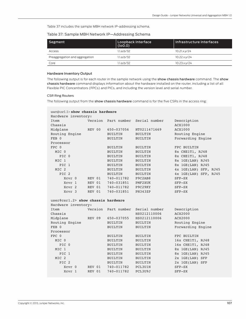
Copyright © 2013, Juniper Networks, Inc. 107
Design Guide - Juniper Networks Universal and Aggregation MBH 1.0
Table 37 includes the sample MBH network IP-addressing schema.
Table 37: Sample MBH Network IP—Addressing Schema
Segment Loopback Interface(lo0.0)
Infrastructure Interfaces
Access 1.1.a.b/32 10.21.x.y/24
Preaggregation and aggregation 1.1.a.b/32 10.22.x.y/24
Core 1.1.a.b/32 10.23.x.y/24
Hardware Inventory Output
The following output is for each router in the sample network using the show chassis hardware command. The show chassis hardware command displays information about the hardware installed on the router, including a list of all
Flexible PIC Concentrators (FPCs) and PICs, and including the version level and serial number.
CSR Ring Routers
The following output from the show chassis hardware command is for the five CSRs in the access ring:
[email protected]> show chassis hardwareHardware inventory:Item Version Part number Serial number DescriptionChassis ACX1000Midplane REV 00 650-037056 HT0211471669 ACX1000Routing Engine BUILTIN BUILTIN Routing EngineFEB 0 BUILTIN BUILTIN Forwarding Engine ProcessorFPC 0 BUILTIN BUILTIN FPC BUILTIN MIC 0 BUILTIN BUILTIN 8x CHE1T1, RJ48 PIC 0 BUILTIN BUILTIN 8x CHE1T1, RJ48 MIC 1 BUILTIN BUILTIN 8x 1GE(LAN) RJ45 PIC 1 BUILTIN BUILTIN 8x 1GE(LAN) RJ45 MIC 2 BUILTIN BUILTIN 4x 1GE(LAN) SFP, RJ45 PIC 2 BUILTIN BUILTIN 4x 1GE(LAN) SFP, RJ45 Xcvr 0 REV 01 740-011782 P9C2AB8 SFP-SX Xcvr 1 REV 01 740-031851 PMF2XUK SFP-SX Xcvr 2 REV 01 740-011782 P9C29KY SFP-SX Xcvr 3 REV 01 740-031851 PN343ZP SFP-SX
[email protected]> show chassis hardwareHardware inventory:Item Version Part number Serial number DescriptionChassis HS0212110006 ACX2000Midplane REV 09 650-037055 HS0212110006 ACX2000Routing Engine BUILTIN BUILTIN Routing EngineFEB 0 BUILTIN BUILTIN Forwarding Engine ProcessorFPC 0 BUILTIN BUILTIN FPC BUILTIN MIC 0 BUILTIN BUILTIN 16x CHE1T1, RJ48 PIC 0 BUILTIN BUILTIN 16x CHE1T1, RJ48 MIC 1 BUILTIN BUILTIN 8x 1GE(LAN) RJ45 PIC 1 BUILTIN BUILTIN 8x 1GE(LAN) RJ45 MIC 2 BUILTIN BUILTIN 2x 1GE(LAN) SFP PIC 2 BUILTIN BUILTIN 2x 1GE(LAN) SFP Xcvr 0 REV 01 740-011782 PCL3U1N SFP-SX Xcvr 1 REV 01 740-011782 PCL3U9J SFP-SX

108 Copyright © 2013, Juniper Networks, Inc.
Design Guide - Juniper Networks Universal and Aggregation MBH 1.0
MIC 3 BUILTIN BUILTIN 2x 10GE(LAN) SFP+ PIC 3 BUILTIN BUILTIN 2x 10GE(LAN) SFP+ Xcvr 0 REV 01 740-031851 PM30KX2 SFP-SX Xcvr 1 REV 01 740-031851 PMF26VG SFP-SX
[email protected]> show chassis hardwareHardware inventory:Item Version Part number Serial number DescriptionChassis ACX2000Midplane REV 00 650-037055 HS0211455197 ACX2000Routing Engine BUILTIN BUILTIN Routing EngineFEB 0 BUILTIN BUILTIN Forwarding Engine ProcessorFPC 0 BUILTIN BUILTIN FPC BUILTIN MIC 0 BUILTIN BUILTIN 16x CHE1T1, RJ48 PIC 0 BUILTIN BUILTIN 16x CHE1T1, RJ48 MIC 1 BUILTIN BUILTIN 8x 1GE(LAN) RJ45 PIC 1 BUILTIN BUILTIN 8x 1GE(LAN) RJ45 MIC 2 BUILTIN BUILTIN 2x 1GE(LAN) SFP PIC 2 BUILTIN BUILTIN 2x 1GE(LAN) SFP Xcvr 0 REV 02 740-011613 PJH4SVC SFP-SX Xcvr 1 REV 02 740-011613 PH10QAE SFP-SX MIC 3 BUILTIN BUILTIN 2x 10GE(LAN) SFP+ PIC 3 BUILTIN BUILTIN 2x 10GE(LAN) SFP+ Xcvr 1 REV 01 740-011613 PD82CZJ SFP-SX
[email protected]> show chassis hardwareHardware inventory:Item Version Part number Serial number DescriptionChassis HT0212110019 ACX1000Midplane REV 09 650-037056 HT0212110019 ACX1000Routing Engine BUILTIN BUILTIN Routing EngineFEB 0 BUILTIN BUILTIN Forwarding Engine ProcessorFPC 0 BUILTIN BUILTIN FPC BUILTIN MIC 0 BUILTIN BUILTIN 8x CHE1T1, RJ48 PIC 0 BUILTIN BUILTIN 8x CHE1T1, RJ48 MIC 1 BUILTIN BUILTIN 8x 1GE(LAN) RJ45 PIC 1 BUILTIN BUILTIN 8x 1GE(LAN) RJ45 MIC 2 BUILTIN BUILTIN 4x 1GE(LAN) SFP, RJ45 PIC 2 BUILTIN BUILTIN 4x 1GE(LAN) SFP, RJ45 Xcvr 0 REV 01 740-031851 PMF15ME SFP-SX Xcvr 1 REV 01 740-031851 PMF2Y0U SFP-SX Xcvr 2 REV 01 740-011613 PDG0UTQ SFP-SX Xcvr 3 REV 01 740-031851 PM30D61 SFP-SX
[email protected]> show chassis hardwareHardware inventory:Item Version Part number Serial number DescriptionChassis HT0212110014 ACX1000Midplane REV 09 650-037056 HT0212110014 ACX1000Routing Engine BUILTIN BUILTIN Routing EngineFEB 0 BUILTIN BUILTIN Forwarding Engine ProcessorFPC 0 BUILTIN BUILTIN FPC BUILTIN MIC 0 BUILTIN BUILTIN 8x CHE1T1, RJ48 PIC 0 BUILTIN BUILTIN 8x CHE1T1, RJ48
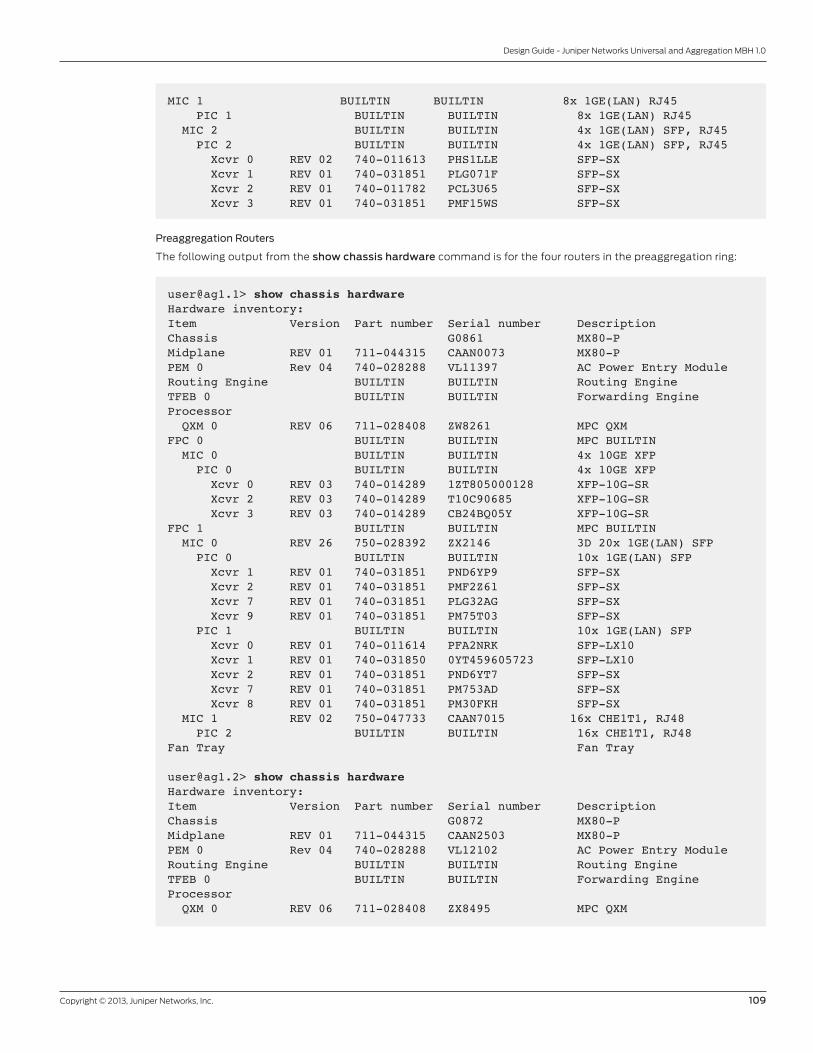
Copyright © 2013, Juniper Networks, Inc. 109
Design Guide - Juniper Networks Universal and Aggregation MBH 1.0
Preaggregation Routers
The following output from the show chassis hardware command is for the four routers in the preaggregation ring:
MIC 1 BUILTIN BUILTIN 8x 1GE(LAN) RJ45 PIC 1 BUILTIN BUILTIN 8x 1GE(LAN) RJ45 MIC 2 BUILTIN BUILTIN 4x 1GE(LAN) SFP, RJ45 PIC 2 BUILTIN BUILTIN 4x 1GE(LAN) SFP, RJ45 Xcvr 0 REV 02 740-011613 PHS1LLE SFP-SX Xcvr 1 REV 01 740-031851 PLG071F SFP-SX Xcvr 2 REV 01 740-011782 PCL3U65 SFP-SX Xcvr 3 REV 01 740-031851 PMF15WS SFP-SX
[email protected]> show chassis hardwareHardware inventory:Item Version Part number Serial number DescriptionChassis G0861 MX80-PMidplane REV 01 711-044315 CAAN0073 MX80-PPEM 0 Rev 04 740-028288 VL11397 AC Power Entry ModuleRouting Engine BUILTIN BUILTIN Routing EngineTFEB 0 BUILTIN BUILTIN Forwarding Engine Processor QXM 0 REV 06 711-028408 ZW8261 MPC QXMFPC 0 BUILTIN BUILTIN MPC BUILTIN MIC 0 BUILTIN BUILTIN 4x 10GE XFP PIC 0 BUILTIN BUILTIN 4x 10GE XFP Xcvr 0 REV 03 740-014289 1ZT805000128 XFP-10G-SR Xcvr 2 REV 03 740-014289 T10C90685 XFP-10G-SR Xcvr 3 REV 03 740-014289 CB24BQ05Y XFP-10G-SRFPC 1 BUILTIN BUILTIN MPC BUILTIN MIC 0 REV 26 750-028392 ZX2146 3D 20x 1GE(LAN) SFP PIC 0 BUILTIN BUILTIN 10x 1GE(LAN) SFP Xcvr 1 REV 01 740-031851 PND6YP9 SFP-SX Xcvr 2 REV 01 740-031851 PMF2Z61 SFP-SX Xcvr 7 REV 01 740-031851 PLG32AG SFP-SX Xcvr 9 REV 01 740-031851 PM75T03 SFP-SX PIC 1 BUILTIN BUILTIN 10x 1GE(LAN) SFP Xcvr 0 REV 01 740-011614 PFA2NRK SFP-LX10 Xcvr 1 REV 01 740-031850 0YT459605723 SFP-LX10 Xcvr 2 REV 01 740-031851 PND6YT7 SFP-SX Xcvr 7 REV 01 740-031851 PM753AD SFP-SX Xcvr 8 REV 01 740-031851 PM30FKH SFP-SX MIC 1 REV 02 750-047733 CAAN7015 16x CHE1T1, RJ48 PIC 2 BUILTIN BUILTIN 16x CHE1T1, RJ48Fan Tray Fan Tray
[email protected]> show chassis hardwareHardware inventory:Item Version Part number Serial number DescriptionChassis G0872 MX80-PMidplane REV 01 711-044315 CAAN2503 MX80-PPEM 0 Rev 04 740-028288 VL12102 AC Power Entry ModuleRouting Engine BUILTIN BUILTIN Routing EngineTFEB 0 BUILTIN BUILTIN Forwarding Engine Processor QXM 0 REV 06 711-028408 ZX8495 MPC QXM
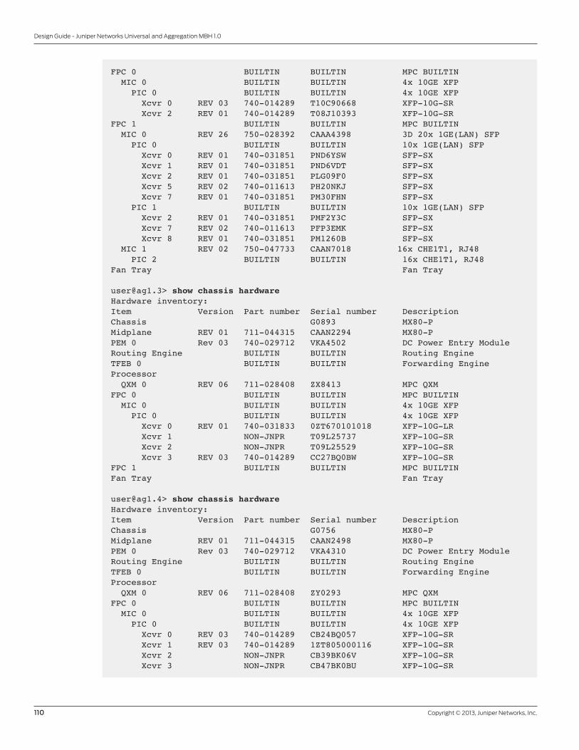
110 Copyright © 2013, Juniper Networks, Inc.
Design Guide - Juniper Networks Universal and Aggregation MBH 1.0
FPC 0 BUILTIN BUILTIN MPC BUILTIN MIC 0 BUILTIN BUILTIN 4x 10GE XFP PIC 0 BUILTIN BUILTIN 4x 10GE XFP Xcvr 0 REV 03 740-014289 T10C90668 XFP-10G-SR Xcvr 2 REV 01 740-014289 T08J10393 XFP-10G-SRFPC 1 BUILTIN BUILTIN MPC BUILTIN MIC 0 REV 26 750-028392 CAAA4398 3D 20x 1GE(LAN) SFP PIC 0 BUILTIN BUILTIN 10x 1GE(LAN) SFP Xcvr 0 REV 01 740-031851 PND6YSW SFP-SX Xcvr 1 REV 01 740-031851 PND6VDT SFP-SX Xcvr 2 REV 01 740-031851 PLG09F0 SFP-SX Xcvr 5 REV 02 740-011613 PH20NKJ SFP-SX Xcvr 7 REV 01 740-031851 PM30FHN SFP-SX PIC 1 BUILTIN BUILTIN 10x 1GE(LAN) SFP Xcvr 2 REV 01 740-031851 PMF2Y3C SFP-SX Xcvr 7 REV 02 740-011613 PFP3EMK SFP-SX Xcvr 8 REV 01 740-031851 PM1260B SFP-SX MIC 1 REV 02 750-047733 CAAN7018 16x CHE1T1, RJ48 PIC 2 BUILTIN BUILTIN 16x CHE1T1, RJ48Fan Tray Fan Tray
[email protected]> show chassis hardware Hardware inventory:Item Version Part number Serial number DescriptionChassis G0893 MX80-PMidplane REV 01 711-044315 CAAN2294 MX80-PPEM 0 Rev 03 740-029712 VKA4502 DC Power Entry ModuleRouting Engine BUILTIN BUILTIN Routing EngineTFEB 0 BUILTIN BUILTIN Forwarding Engine Processor QXM 0 REV 06 711-028408 ZX8413 MPC QXMFPC 0 BUILTIN BUILTIN MPC BUILTIN MIC 0 BUILTIN BUILTIN 4x 10GE XFP PIC 0 BUILTIN BUILTIN 4x 10GE XFP Xcvr 0 REV 01 740-031833 0ZT670101018 XFP-10G-LR Xcvr 1 NON-JNPR T09L25737 XFP-10G-SR Xcvr 2 NON-JNPR T09L25529 XFP-10G-SR Xcvr 3 REV 03 740-014289 CC27BQ0BW XFP-10G-SRFPC 1 BUILTIN BUILTIN MPC BUILTINFan Tray Fan Tray
[email protected]> show chassis hardware Hardware inventory:Item Version Part number Serial number DescriptionChassis G0756 MX80-PMidplane REV 01 711-044315 CAAN2498 MX80-PPEM 0 Rev 03 740-029712 VKA4310 DC Power Entry ModuleRouting Engine BUILTIN BUILTIN Routing EngineTFEB 0 BUILTIN BUILTIN Forwarding Engine Processor QXM 0 REV 06 711-028408 ZY0293 MPC QXMFPC 0 BUILTIN BUILTIN MPC BUILTIN MIC 0 BUILTIN BUILTIN 4x 10GE XFP PIC 0 BUILTIN BUILTIN 4x 10GE XFP Xcvr 0 REV 03 740-014289 CB24BQ057 XFP-10G-SR Xcvr 1 REV 03 740-014289 1ZT805000116 XFP-10G-SR Xcvr 2 NON-JNPR CB39BK06V XFP-10G-SR Xcvr 3 NON-JNPR CB47BK0BU XFP-10G-SR
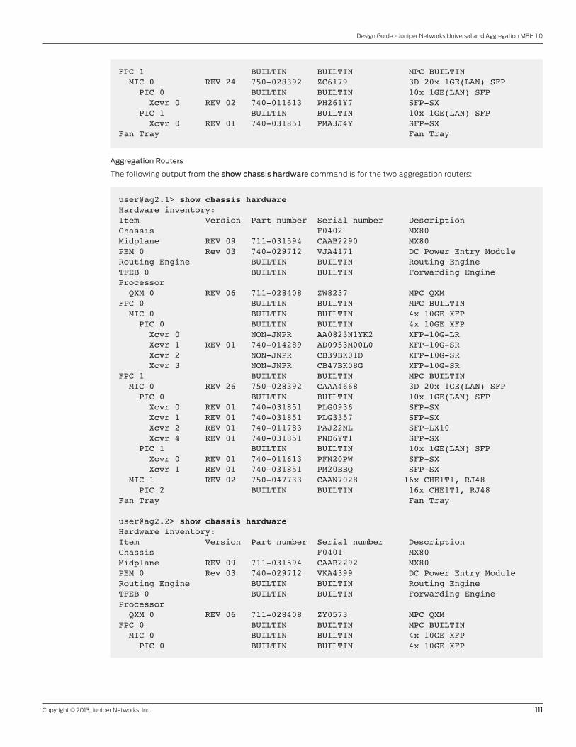
Copyright © 2013, Juniper Networks, Inc. 111
Design Guide - Juniper Networks Universal and Aggregation MBH 1.0
FPC 1 BUILTIN BUILTIN MPC BUILTIN MIC 0 REV 24 750-028392 ZC6179 3D 20x 1GE(LAN) SFP PIC 0 BUILTIN BUILTIN 10x 1GE(LAN) SFP Xcvr 0 REV 02 740-011613 PH261Y7 SFP-SX PIC 1 BUILTIN BUILTIN 10x 1GE(LAN) SFP Xcvr 0 REV 01 740-031851 PMA3J4Y SFP-SXFan Tray Fan Tray
Aggregation Routers
The following output from the show chassis hardware command is for the two aggregation routers:
[email protected]> show chassis hardwareHardware inventory:Item Version Part number Serial number DescriptionChassis F0402 MX80Midplane REV 09 711-031594 CAAB2290 MX80PEM 0 Rev 03 740-029712 VJA4171 DC Power Entry ModuleRouting Engine BUILTIN BUILTIN Routing EngineTFEB 0 BUILTIN BUILTIN Forwarding Engine Processor QXM 0 REV 06 711-028408 ZW8237 MPC QXMFPC 0 BUILTIN BUILTIN MPC BUILTIN MIC 0 BUILTIN BUILTIN 4x 10GE XFP PIC 0 BUILTIN BUILTIN 4x 10GE XFP Xcvr 0 NON-JNPR AA0823N1YK2 XFP-10G-LR Xcvr 1 REV 01 740-014289 AD0953M00L0 XFP-10G-SR Xcvr 2 NON-JNPR CB39BK01D XFP-10G-SR Xcvr 3 NON-JNPR CB47BK08G XFP-10G-SRFPC 1 BUILTIN BUILTIN MPC BUILTIN MIC 0 REV 26 750-028392 CAAA4668 3D 20x 1GE(LAN) SFP PIC 0 BUILTIN BUILTIN 10x 1GE(LAN) SFP Xcvr 0 REV 01 740-031851 PLG0936 SFP-SX Xcvr 1 REV 01 740-031851 PLG3357 SFP-SX Xcvr 2 REV 01 740-011783 PAJ22NL SFP-LX10 Xcvr 4 REV 01 740-031851 PND6YT1 SFP-SX PIC 1 BUILTIN BUILTIN 10x 1GE(LAN) SFP Xcvr 0 REV 01 740-011613 PFN20PW SFP-SX Xcvr 1 REV 01 740-031851 PM20BBQ SFP-SX MIC 1 REV 02 750-047733 CAAN7028 16x CHE1T1, RJ48 PIC 2 BUILTIN BUILTIN 16x CHE1T1, RJ48Fan Tray Fan Tray
[email protected]> show chassis hardware Hardware inventory:Item Version Part number Serial number DescriptionChassis F0401 MX80Midplane REV 09 711-031594 CAAB2292 MX80PEM 0 Rev 03 740-029712 VKA4399 DC Power Entry ModuleRouting Engine BUILTIN BUILTIN Routing EngineTFEB 0 BUILTIN BUILTIN Forwarding Engine Processor QXM 0 REV 06 711-028408 ZY0573 MPC QXMFPC 0 BUILTIN BUILTIN MPC BUILTIN MIC 0 BUILTIN BUILTIN 4x 10GE XFP PIC 0 BUILTIN BUILTIN 4x 10GE XFP
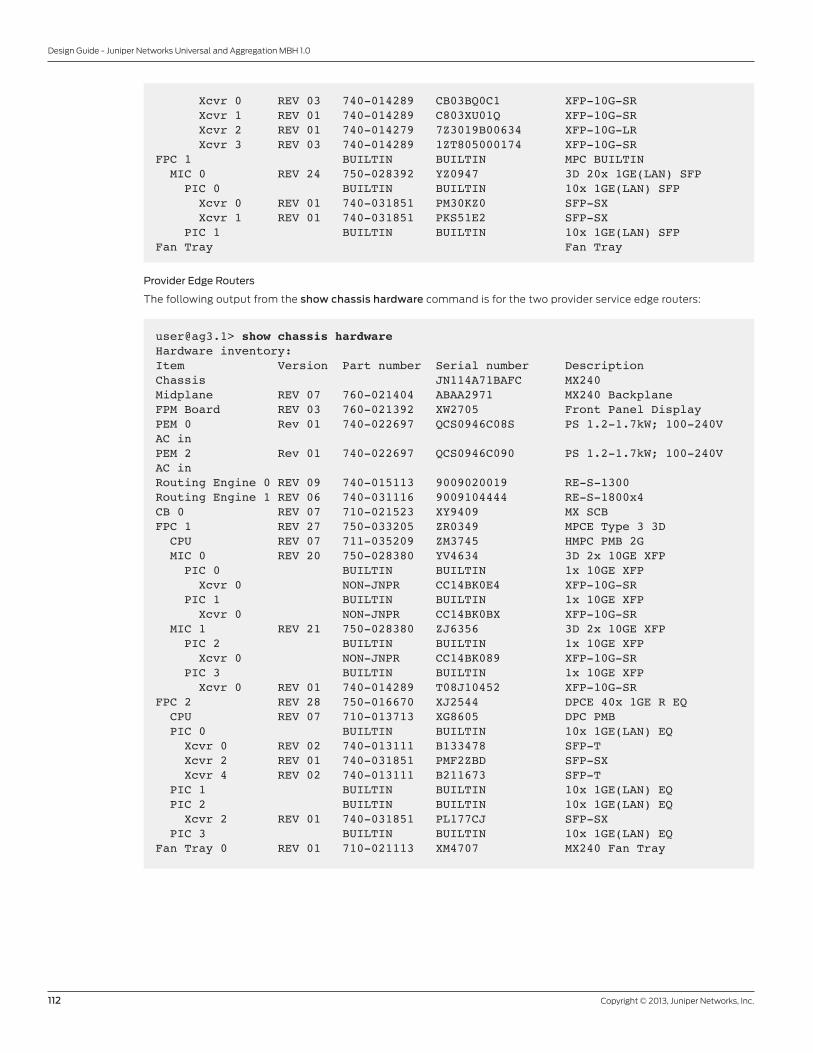
112 Copyright © 2013, Juniper Networks, Inc.
Design Guide - Juniper Networks Universal and Aggregation MBH 1.0
Xcvr 0 REV 03 740-014289 CB03BQ0C1 XFP-10G-SR Xcvr 1 REV 01 740-014289 C803XU01Q XFP-10G-SR Xcvr 2 REV 01 740-014279 7Z3019B00634 XFP-10G-LR Xcvr 3 REV 03 740-014289 1ZT805000174 XFP-10G-SRFPC 1 BUILTIN BUILTIN MPC BUILTIN MIC 0 REV 24 750-028392 YZ0947 3D 20x 1GE(LAN) SFP PIC 0 BUILTIN BUILTIN 10x 1GE(LAN) SFP Xcvr 0 REV 01 740-031851 PM30KZ0 SFP-SX Xcvr 1 REV 01 740-031851 PKS51E2 SFP-SX PIC 1 BUILTIN BUILTIN 10x 1GE(LAN) SFPFan Tray Fan Tray
Provider Edge Routers
The following output from the show chassis hardware command is for the two provider service edge routers:
[email protected]> show chassis hardwareHardware inventory:Item Version Part number Serial number DescriptionChassis JN114A71BAFC MX240Midplane REV 07 760-021404 ABAA2971 MX240 BackplaneFPM Board REV 03 760-021392 XW2705 Front Panel DisplayPEM 0 Rev 01 740-022697 QCS0946C08S PS 1.2-1.7kW; 100-240V AC inPEM 2 Rev 01 740-022697 QCS0946C090 PS 1.2-1.7kW; 100-240V AC inRouting Engine 0 REV 09 740-015113 9009020019 RE-S-1300Routing Engine 1 REV 06 740-031116 9009104444 RE-S-1800x4CB 0 REV 07 710-021523 XY9409 MX SCBFPC 1 REV 27 750-033205 ZR0349 MPCE Type 3 3D CPU REV 07 711-035209 ZM3745 HMPC PMB 2G MIC 0 REV 20 750-028380 YV4634 3D 2x 10GE XFP PIC 0 BUILTIN BUILTIN 1x 10GE XFP Xcvr 0 NON-JNPR CC14BK0E4 XFP-10G-SR PIC 1 BUILTIN BUILTIN 1x 10GE XFP Xcvr 0 NON-JNPR CC14BK0BX XFP-10G-SR MIC 1 REV 21 750-028380 ZJ6356 3D 2x 10GE XFP PIC 2 BUILTIN BUILTIN 1x 10GE XFP Xcvr 0 NON-JNPR CC14BK089 XFP-10G-SR PIC 3 BUILTIN BUILTIN 1x 10GE XFP Xcvr 0 REV 01 740-014289 T08J10452 XFP-10G-SRFPC 2 REV 28 750-016670 XJ2544 DPCE 40x 1GE R EQ CPU REV 07 710-013713 XG8605 DPC PMB PIC 0 BUILTIN BUILTIN 10x 1GE(LAN) EQ Xcvr 0 REV 02 740-013111 B133478 SFP-T Xcvr 2 REV 01 740-031851 PMF2ZBD SFP-SX Xcvr 4 REV 02 740-013111 B211673 SFP-T PIC 1 BUILTIN BUILTIN 10x 1GE(LAN) EQ PIC 2 BUILTIN BUILTIN 10x 1GE(LAN) EQ Xcvr 2 REV 01 740-031851 PL177CJ SFP-SX PIC 3 BUILTIN BUILTIN 10x 1GE(LAN) EQFan Tray 0 REV 01 710-021113 XM4707 MX240 Fan Tray
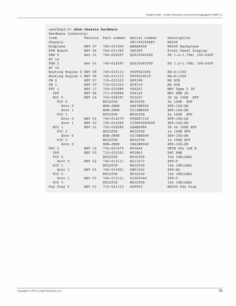
Copyright © 2013, Juniper Networks, Inc. 113
Design Guide - Juniper Networks Universal and Aggregation MBH 1.0
[email protected]> show chassis hardware Hardware inventory:Item Version Part number Serial number DescriptionChassis JN1194255AFC MX240Midplane REV 07 760-021404 ABAA8658 MX240 BackplaneFPM Board REV 04 760-021392 YA0369 Front Panel DisplayPEM 0 Rev 01 740-022697 QCS1004C062 PS 1.2-1.7kW; 100-240V AC inPEM 2 Rev 01 740-022697 QCS1004C05P PS 1.2-1.7kW; 100-240V AC inRouting Engine 0 REV 09 740-015113 9009023694 RE-S-1300Routing Engine 1 REV 09 740-015113 9009020019 RE-S-1300CB 0 REV 07 710-021523 XZ9398 MX SCBCB 1 REV 03 710-021523 XC9314 MX SCBFPC 1 REV 17 750-031089 YZ6247 MPC Type 2 3D CPU REV 06 711-030884 YX4120 MPC PMB 2G MIC 0 REV 24 750-028387 YC3247 3D 4x 10GE XFP PIC 0 BUILTIN BUILTIN 2x 10GE XFP Xcvr 0 NON-JNPR CB47BK05U XFP-10G-SR Xcvr 1 NON-JNPR CC14BK05S XFP-10G-SR PIC 1 BUILTIN BUILTIN 2x 10GE XFP Xcvr 0 REV 01 740-014279 T08D87316 XFP-10G-LR Xcvr 1 REV 03 740-014289 21T805000059 XFP-10G-SR MIC 1 REV 21 750-028380 CAAE6986 3D 2x 10GE XFP PIC 2 BUILTIN BUILTIN 1x 10GE XFP Xcvr 0 NON-JNPR CC14BK069 XFP-10G-SR PIC 3 BUILTIN BUILTIN 1x 10GE XFP Xcvr 0 NON-JNPR CB42BK04D XFP-10G-SRFPC 2 REV 12 750-021679 WY3644 DPCE 40x 1GE R CPU REV 03 710-022351 WY2863 DPC PMB PIC 0 BUILTIN BUILTIN 10x 1GE(LAN) Xcvr 0 REV 02 740-013111 B211675 SFP-T PIC 1 BUILTIN BUILTIN 10x 1GE(LAN) Xcvr 1 REV 01 740-031851 PMF1622 SFP-SX PIC 2 BUILTIN BUILTIN 10x 1GE(LAN) Xcvr 1 REV 01 740-013111 62362044 SFP-T PIC 3 BUILTIN BUILTIN 10x 1GE(LAN)Fan Tray 0 REV 01 710-021113 XX9503 MX240 Fan Tray
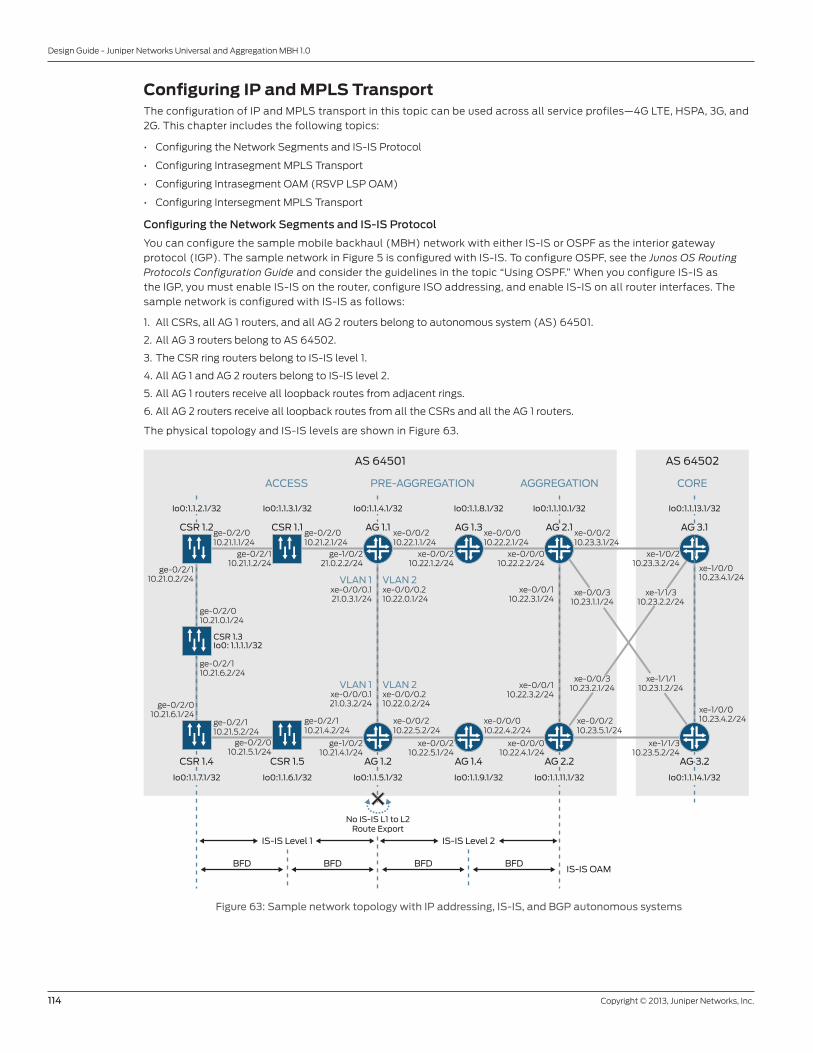
114 Copyright © 2013, Juniper Networks, Inc.
Design Guide - Juniper Networks Universal and Aggregation MBH 1.0
Configuring IP and MPLS TransportThe configuration of IP and MPLS transport in this topic can be used across all service profiles—4G LTE, HSPA, 3G, and
2G. This chapter includes the following topics:
• Configuring the Network Segments and IS-IS Protocol
• Configuring Intrasegment MPLS Transport
• Configuring Intrasegment OAM (RSVP LSP OAM)
• Configuring Intersegment MPLS Transport
Configuring the Network Segments and IS-IS Protocol
You can configure the sample mobile backhaul (MBH) network with either IS-IS or OSPF as the interior gateway
protocol (IGP). The sample network in Figure 5 is configured with IS-IS. To configure OSPF, see the Junos OS Routing
Protocols Configuration Guide and consider the guidelines in the topic “Using OSPF.” When you configure IS-IS as
the IGP, you must enable IS-IS on the router, configure ISO addressing, and enable IS-IS on all router interfaces. The
sample network is configured with IS-IS as follows:
1. All CSRs, all AG 1 routers, and all AG 2 routers belong to autonomous system (AS) 64501.
2. All AG 3 routers belong to AS 64502.
3. The CSR ring routers belong to IS-IS level 1.
4. All AG 1 and AG 2 routers belong to IS-IS level 2.
5. All AG 1 routers receive all loopback routes from adjacent rings.
6. All AG 2 routers receive all loopback routes from all the CSRs and all the AG 1 routers.
The physical topology and IS-IS levels are shown in Figure 63.
ACCESS COREAGGREGATIONPRE-AGGREGATION
CSR 1.3Io0: 1.1.1.1/32
Io0:1.1.3.1/32 Io0:1.1.8.1/32
Io0:1.1.6.1/32 Io0:1.1.9.1/32
AG 1.3AG 1.1 AG 2.1
AG 1.4 AG 2.2AG 1.2
CSR 1.2
CSR 1.4
AG 3.1
AG 3.2
ge-0/2/0
ge-0/2/110.21.1.1/24
10.21.1.2/24
ge-0/2/0
ge-1/0/210.21.2.1/24
21.0.2.2/24
xe-0/0/2
xe-0/0/210.22.1.1/24
10.22.1.2/24
VLAN 1
VLAN 1
xe-0/0/0.121.0.3.1/24
xe-0/0/0.121.0.3.2/24
VLAN 2
VLAN 2
xe-0/0/0.210.22.0.1/24
xe-0/0/0.210.22.0.2/24
ge-0/2/1
ge-1/0/2
10.21.4.2/24
10.21.4.1/24ge-0/2/0
10.21.5.1/24
ge-0/2/010.21.0.1/24
ge-0/2/110.21.0.2/24
ge-0/2/010.21.6.1/24
ge-0/2/110.21.5.2/24
ge-0/2/110.21.6.2/24
xe-0/0/2
xe-0/0/2
10.22.5.2/24
10.22.5.1/24
xe-0/0/0
xe-0/0/010.22.2.1/24
10.22.2.2/24
xe-0/0/110.22.3.1/24
xe-0/0/110.22.3.2/24
xe-0/0/0
xe-0/0/0
10.22.4.2/24
10.22.4.1/24
xe-0/0/2
xe-1/0/210.23.3.1/24
10.23.3.2/24
xe-0/0/2
xe-1/1/3
10.23.5.1/24
10.23.5.2/24
IS-IS Level 1 IS-IS Level 2
IS-IS OAMBFD BFD BFDBFD
No IS-IS L1 to L2Route Export
AS 64501 AS 64502
CSR 1.1
CSR 1.5
Io0:1.1.4.1/32 Io0:1.1.10.1/32Io0:1.1.2.1/32 Io0:1.1.13.1/32
Io0:1.1.5.1/32 Io0:1.1.11.1/32Io0:1.1.7.1/32 Io0:1.1.14.1/32
xe-1/0/010.23.4.1/24
xe-1/0/010.23.4.2/24
xe-1/1/110.23.1.2/24
xe-1/1/310.23.2.2/24
xe-0/0/310.23.1.1/24
xe-0/0/310.23.2.1/24
Figure 63: Sample network topology with IP addressing, IS-IS, and BGP autonomous systems
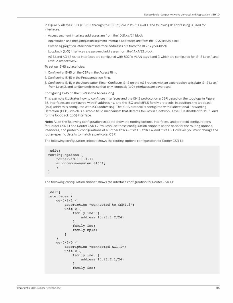
Copyright © 2013, Juniper Networks, Inc. 115
Design Guide - Juniper Networks Universal and Aggregation MBH 1.0
In Figure 5, all the CSRs (CSR 1.1 through to CSR 1.5) are in IS-IS Level 1. The following IP addressing is used for
interfaces:
• Access segment interface addresses are from the 10.21.x.y/24 block
• Aggregation and preaggregation segment interface addresses are from the 10.22.x.y/24 block
• Core to aggregation interconnect interface addresses are from the 10.23.x.y/24 block
• Loopback (lo0) interfaces are assigned addresses from the 1.1.x.1/32 block
• AG 1.1 and AG 1.2 router interfaces are configured with 802.1q VLAN tags 1 and 2, which are configured for IS-IS Level 1 and
Level 2, respectively.
To set up IS-IS adjacencies:
1. Configuring IS-IS on the CSRs in the Access Ring.
2. Configuring IS-IS in the Preaggregation Ring.
3. Configuring IS-IS in the Aggregation Ring—Configure IS-IS on the AG 1 routers with an export policy to isolate IS-IS Level 1 from Level 2, and to filter prefixes so that only loopback (lo0) interfaces are advertised.
Configuring IS-IS on the CSRs in the Access Ring
This example illustrates how to configure interfaces and the IS-IS protocol on a CSR based on the topology in Figure
63. Interfaces are configured with IP addressing, and the ISO and MPLS family protocols. In addition, the loopback
(lo0) address is configured with ISO addressing. The IS-IS protocol is configured with Bidirectional Forwarding
Detection (BFD), which is a simple hello mechanism that detects failures in a network. Level 2 is disabled for IS-IS and
for the loopback (lo0) interface.
Note: All of the following configuration snippets show the routing options, interfaces, and protocol configurations
for Router CSR 1.1 and Router CSR 1.2. You can use these configuration snippets as the basis for the routing options,
interfaces, and protocol configurations of all other CSRs—CSR 1.3, CSR 1.4, and CSR 1.5. However, you must change the
router-specific details to match a particular CSR.
The following configuration snippet shows the routing-options configuration for Router CSR 1.1:
[edit]routing-options { router-id 1.1.3.1; autonomous-system 64501; }}
The following configuration snippet shows the interface configuration for Router CSR 1.1:
[edit]interfaces { ge-0/2/1 { description “connected to CSR1.2”; unit 0 { family inet { address 10.21.1.2/24; } family iso; family mpls; } } ge-0/2/0 { description “connected AG1.1”; unit 0 { family inet { address 10.21.2.1/24; } family iso;

116 Copyright © 2013, Juniper Networks, Inc.
Design Guide - Juniper Networks Universal and Aggregation MBH 1.0
family mpls; } } lo0 { unit 0 { family inet { address 1.1.3.1/32; } family iso { address 47.0005.0010.0100.3001.00; } } }}
The following configuration snippet shows the IS-IS protocol configuration for Router CSR 1.1. The BFD liveness
detection values allow a failure detection time of 30 ms. Even though IS-IS session failure must be detected as quickly
as possible, there are scalability issues, resulting in the minimum interval verified with our solution as 10 ms.
[edit]protocols { isis { level 2 disable; interface ge-0/2/0.0 { bfd-liveness-detection { minimum-interval 100; multiplier 3; no-adaptation; } level 2 disable; } interface ge-0/2/1.0 { bfd-liveness-detection { minimum-interval 10; multiplier 3; no-adaptation; } level 2 disable; } interface lo0.0 { passive; level 2 disable; } }}
The following configuration snippet shows the routing-options configuration for Router CSR 1.2:
[edit]
routing-options {
router-id 1.1.2.1;
autonomous-system 64501;
}
}

Copyright © 2013, Juniper Networks, Inc. 117
Design Guide - Juniper Networks Universal and Aggregation MBH 1.0
The following configuration snippet shows the interface configuration for Router CSR 1.2:
[edit]interfaces { ge-0/2/0 { description “connected CSR1.1”; unit 0 { family inet { address 10.21.1.1/24; } family iso; family mpls; } } ge-0/2/1 { description “connected to CSR1.3”; enable; unit 0 { family inet { address 10.21.0.2/24; } family iso; family mpls; } } lo0 { unit 0 { family inet { address 1.1.2.1/32; } family iso { address 47.0005.0010.0100.2001.00; } } }}
The following configuration snippet shows the IS-IS protocol configuration for Router CSR 1.2:
[edit]protocols { isis { level 2 disable; interface ge-0/2/0.0 { bfd-liveness-detection { minimum-interval 10; multiplier 3; no-adaptation; } } interface ge-0/2/1.0 { bfd-liveness-detection { minimum-interval 10; multiplier 3; no-adaptation; } }
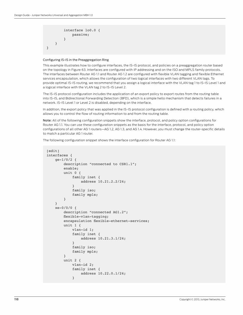
118 Copyright © 2013, Juniper Networks, Inc.
Design Guide - Juniper Networks Universal and Aggregation MBH 1.0
interface lo0.0 { passive; } }}
Configuring IS-IS in the Preaggregation Ring
This example illustrates how to configure interfaces, the IS-IS protocol, and policies on a preaggregation router based
on the topology in Figure 63. Interfaces are configured with IP addressing and on the ISO and MPLS family protocols.
The interfaces between Router AG 1.1 and Router AG 1.2 are configured with flexible VLAN tagging and flexible Ethernet
services encapsulation, which allows the configuration of two logical interfaces with two different VLAN tags. To
provide optimal IS-IS routing, we recommend that you assign a logical interface with the VLAN tag 1 to IS-IS Level 1 and
a logical interface with the VLAN tag 2 to IS-IS Level 2.
The IS-IS protocol configuration includes the application of an export policy to export routes from the routing table
into IS-IS, and Bidirectional Forwarding Detection (BFD), which is a simple hello mechanism that detects failures in a
network. IS-IS Level 1 or Level 2 is disabled, depending on the interface.
In addition, the export policy that was applied in the IS-IS protocol configuration is defined with a routing policy, which
allows you to control the flow of routing information to and from the routing table.
Note: All of the following configuration snippets show the interface, protocol, and policy option configurations for
Router AG 1.1. You can use these configuration snippets as the basis for the interface, protocol, and policy option
configurations of all other AG 1 routers—AG 1.2, AG 1.3, and AG 1.4. However, you must change the router-specific details
to match a particular AG 1 router.
The following configuration snippet shows the interface configuration for Router AG 1.1:
[edit]interfaces { ge-1/0/2 { description “connected to CSR1.1”; enable; unit 0 { family inet { address 10.21.2.2/24; } family iso; family mpls; } } xe-0/0/0 { description “connected AG1.2”; flexible-vlan-tagging; encapsulation flexible-ethernet-services; unit 1 { vlan-id 1; family inet { address 10.21.3.1/24; } family iso; family mpls; } unit 2 { vlan-id 2; family inet { address 10.22.0.1/24; }

Copyright © 2013, Juniper Networks, Inc. 119
Design Guide - Juniper Networks Universal and Aggregation MBH 1.0
family iso; family mpls; } } xe-0/0/2 { description “connected AG1.3”; unit 0 { family inet { address 10.22.1.1/24; } family iso; family mpls; } } lo0 { unit 0 { family inet { address 1.1.4.1/32; } family iso { address 47.0005.0010.0100.4001.00; } } }}
The following configuration snippet shows the IS-IS protocol configuration for Router AG 1.1:
[edit]protocols { isis { export isis-export; interface ge-1/0/2.0 { bfd-liveness-detection { minimum-interval 10; multiplier 3; no-adaptation; } level 2 disable; } interface xe-0/0/0.1 { level 2 disable; bfd-liveness-detection { minimum-interval 10; multiplier 3; no-adaptation; } } interface xe-0/0/0.2 { level 1 disable; bfd-liveness-detection { minimum-interval 10; multiplier 3; no-adaptation; } }
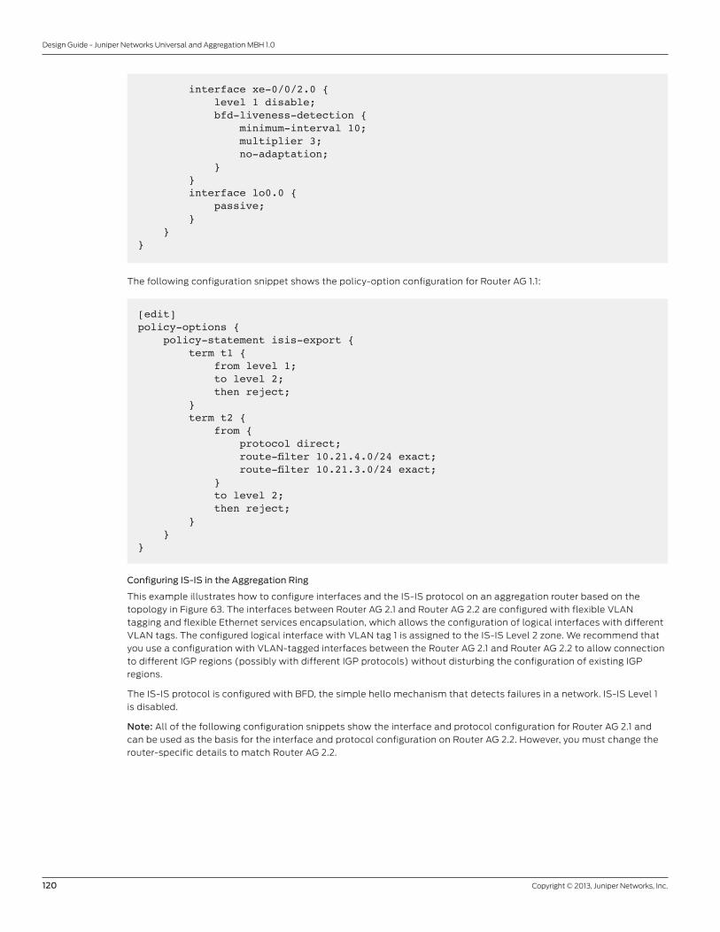
120 Copyright © 2013, Juniper Networks, Inc.
Design Guide - Juniper Networks Universal and Aggregation MBH 1.0
interface xe-0/0/2.0 { level 1 disable; bfd-liveness-detection { minimum-interval 10; multiplier 3; no-adaptation; } } interface lo0.0 { passive; } }}
The following configuration snippet shows the policy-option configuration for Router AG 1.1:
[edit]policy-options { policy-statement isis-export { term t1 { from level 1; to level 2; then reject; } term t2 { from { protocol direct; route-filter 10.21.4.0/24 exact; route-filter 10.21.3.0/24 exact; } to level 2; then reject; } }}
Configuring IS-IS in the Aggregation Ring
This example illustrates how to configure interfaces and the IS-IS protocol on an aggregation router based on the
topology in Figure 63. The interfaces between Router AG 2.1 and Router AG 2.2 are configured with flexible VLAN
tagging and flexible Ethernet services encapsulation, which allows the configuration of logical interfaces with different
VLAN tags. The configured logical interface with VLAN tag 1 is assigned to the IS-IS Level 2 zone. We recommend that
you use a configuration with VLAN-tagged interfaces between the Router AG 2.1 and Router AG 2.2 to allow connection
to different IGP regions (possibly with different IGP protocols) without disturbing the configuration of existing IGP
regions.
The IS-IS protocol is configured with BFD, the simple hello mechanism that detects failures in a network. IS-IS Level 1
is disabled.
Note: All of the following configuration snippets show the interface and protocol configuration for Router AG 2.1 and
can be used as the basis for the interface and protocol configuration on Router AG 2.2. However, you must change the
router-specific details to match Router AG 2.2.

Copyright © 2013, Juniper Networks, Inc. 121
Design Guide - Juniper Networks Universal and Aggregation MBH 1.0
This configuration snippet shows the interface configuration for Router AG 2.1:
[edit]interfaces { xe-0/0/0 { description “connected to AG1.3”; enable; unit 0 { family inet { address 10.22.2.2/24; } family iso; family mpls; } } xe-0/0/1 { description “connected to AG2.2”; flexible-vlan-tagging; encapsulation flexible-ethernet-services; unit 1 { vlan-id 1; family inet { address 10.22.3.1/24; } family iso; family mpls; } } xe-0/0/2 { description “connected to AG3.1”; unit 0 { family inet { address 10.23.3.1/24; } family iso; family mpls; } } xe-0/0/3 { description “connected to AG3.2”; unit 0 { family inet { address 10.23.1.1/24; } family iso; family mpls; } } lo0 { unit 0 { family inet { address 1.1.10.1/32; } family iso { address 47.0005.0010.0101.0001.00; } } }}
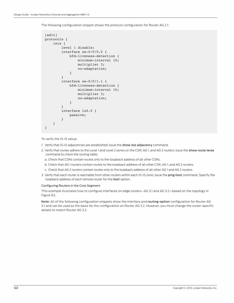
122 Copyright © 2013, Juniper Networks, Inc.
Design Guide - Juniper Networks Universal and Aggregation MBH 1.0
The following configuration snippet shows the protocol configuration for Router AG 2.1:
[edit]protocols { isis { level 1 disable; interface xe-0/0/0.0 { bfd-liveness-detection { minimum-interval 10; multiplier 3; no-adaptation; } } interface xe-0/0/1.1 { bfd-liveness-detection { minimum-interval 10; multiplier 3; no-adaptation; } } interface lo0.0 { passive; } }}
To verify the IS-IS setup:
1. Verify that IS-IS adjacencies are established; issue the show isis adjacency command.
2. Verify that routes adhere to the Level 1 and Level 2 zones on the CSR, AG 1, and AG 2 routers; issue the show route terse command to check the routing table.
a. Check that CSRs contain routes only to the loopback address of all other CSRs.
b. Check that AG 1 routers contain routes to the loopback address of all other CSR, AG 1, and AG 2 routers.
c. Check that AG 2 routers contain routes only to the loopback address of all other AG 1 and AG 2 routers.
3. Verify that each router is reachable from other routers within each IS-IS zone; issue the ping host command. Specify the
loopback address of each remote router for the host option.
Configuring Routers in the Core Segment
This example illustrates how to configure interfaces on edge routers—AG 3.1 and AG 3.2—based on the topology in
Figure 63.
Note: All of the following configuration snippets show the interface and routing-option configuration for Router AG
3.1 and can be used as the basis for the configuration on Router AG 3.2. However, you must change the router-specific
details to match Router AG 3.2.

Copyright © 2013, Juniper Networks, Inc. 123
Design Guide - Juniper Networks Universal and Aggregation MBH 1.0
[edit]interfaces { xe-1/0/0 { unit 0 { family inet { address 10.23.4.1/24; } family iso; family mpls; } } xe-1/0/2 { unit 0 { family inet { address 10.23.3.2/24; } family iso; family mpls; } } xe-1/1/3 { unit 0 { family inet { address 10.23.2.2/24; } family iso; family mpls; } } lo0 { unit 0 { family inet { address 1.1.13.1/32; } family iso { address 47.0006.0010.0101.3001.00; } family mpls; } }}
[edit]routing-options { router-id 1.1.13.1; autonomous-system 64502;}

124 Copyright © 2013, Juniper Networks, Inc.
Design Guide - Juniper Networks Universal and Aggregation MBH 1.0
Configuring Intrasegment MPLS Transport
This example illustrates how to configure end-to-end MPLS transport on routers in different segments of the MBH
network, including the configuration of RSVP, MPLS label-switched paths, MPLS fast reroute (FRR), primary, and
secondary paths as shown in Figure 64.
ACCESS COREPRE-AGGREGATION AGGREGATION
CSR 1.3
AS 64501
PrimaryPath
SecondaryPath
AS 64502
Io0: 1.1.1.1/32
Io0:1.1.3.1/32 Io0:1.1.8.1/32
Io0:1.1.6.1/32 Io0:1.1.9.1/32
CSR 1.1 AG 1.3AG 1.1 AG 2.1
CSR 1.5 AG 1.4 AG 2.2AG 1.2
CSR 1.2
CSR 1.4
AG 3.1
AG 3.2
RSVP LSP (Primary Path)
RSVP LSP (Secondary Path)
RSVP LSP (Primary Path)
RSVP LSP (Secondary Path)
BFDBFD
ge-0/2/0
ge-0/2/110.21.1.1/24
10.21.1.2/24
ge-0/2/0
ge-1/0/210.21.2.1/24
10.21.2.2/24
xe-0/0/2
xe-0/0/210.22.1.1/24
10.22.1.2/24
VLAN 1
VLAN 1
xe-0/0/0.110.21.3.1/24
xe-0/0/0.121.0.3.2/24
VLAN 2
VLAN 2
xe-0/0/0.210.22.0.1/24
xe-0/0/0.210.22.0.2/24
ge-0/2/1
ge-1/0/210.21.4.2/24
10.21.4.1/24ge-0/2/0
10.21.5.1/24
ge-0/2/010.21.0.1/24
ge-0/2/110.21.0.2/24
ge-0/2/010.21.6.1/24
ge-0/2/110.21.5.2/24
ge-0/2/110.21.6.2/24
xe-0/0/2
xe-0/0/2
10.22.5.2/24
10.22.5.1/24
xe-0/0/0
xe-0/0/010.22.2.1/24
10.22.2.2/24
xe-0/0/0
xe-0/0/010.22.4.2/24
10.22.4.1/24
xe-0/0/2
xe-1/0/2
xe-1/0/010.23.4.1/24
xe-1/0/010.23.4.2/24
10.23.3.1/24
10.23.3.2/24
xe-0/0/2
xe-1/1/310.23.5.1/24
10.23.5.2/24
Partial Mesh RSVP Full Mesh RSVP
MPLS OAMBFDBFD
MPLSFast
Reroute
MPLSFast
Reroute
Io0: 1.1.4.1/32 Io0:1.1.10.1/32Io0:1.1.2.1/32 Io0:1.1.13.1/32
Io0:1.1.5.1/32 Io0:1.1.11.1/32Io0:1.1.7.1/32 Io0:1.1.14.1/32
xe-0/0/110.22.3.1/24
xe-0/0/110.22.3.2/24
xe-0/0/310.23.1.1/24
xe-1/1/110.23.1.2/24
xe-0/0/310.23.2.1/24
xe-1/1/310.23.2.2/24
Figure 64: Intrasegment MPLS deployment
To configure an intrasegment RSVP LSP and an intersegment LSP based on the topology in Figure 64:
1. Configure an RSVP LSP between each CSR and Router AG 1.1 and Router AG 1.2:
a. Configure two RSVP LSPs from each CSR to Router AG 1.1 and Router AG 1.2 and vice versa.
b. Configure path protection with the primary path going in one direction and the secondary path going in the opposite direction.
c. Configure the secondary path as the standby path.
d. Configure LDP tunneling.
e. Configure the BFD protocol for fast end-to-end LSP failure detection.
2. Configure an RSVP LSP between each AG 1 and AG 2 router:
a. Configure RSVP LSPs between each AG 1 and AG 2 router.
b. Configure path protection with the primary path going in one direction and the secondary path going in the opposite direction.
c. Configure the secondary path as the standby path.
3. Configure per-packet load balancing on all routers.
All of the following configuration snippets for the CSR, AG 1, and AG 2 routers are the result of Steps 1 through 3 of
Configuring Intrasegment MPLS Transport.

Copyright © 2013, Juniper Networks, Inc. 125
Design Guide - Juniper Networks Universal and Aggregation MBH 1.0
Note: The following configuration snippets show the MPLS configuration for Router CSR 1.1 and Router CSR 1.2. You can
use these configuration snippets as the basis for the MPLS configuration of all other CSRs—CSR 1.3, CSR 1.4, and CSR
1.5. However, you must change the router-specific details to match a particular CSR.
The following configuration snippet shows the MPLS configuration for Router CSR 1.1:
[edit]protocols { rsvp { interface ge-0/2/1.0; interface ge-0/2/0.0; } mpls { label-switched-path csr1.1_to_ag1.1 { from 1.1.3.1; to 1.1.4.1; ldp-tunneling;fast-reroute; primary via-ag1.1; secondary via-csr1.2; } label-switched-path csr1.1_to_ag1.2 { from 1.1.3.1; to 1.1.5.1; ldp-tunneling; fast-reroute; primary via-ag1.1; secondary via-csr1.2; } path via-ag1.1 { 10.21.2.2 strict; } path via-csr1.2 { 10.21.1.1 strict; } interface ge-0/2/1.0; interface ge-0/2/0.0; interface lo0.0; } ldp { interface lo0.0; }}
The following configuration snippet shows the MPLS configuration for Router CSR 1.2:
[edit]protocols { rsvp { interface ge-0/2/1.0; interface ge-0/2/0.0; } mpls { label-switched-path csr1.2_to_ag1.1 { from 1.1.2.1; to 1.1.4.1; ldp-tunneling; fast-reroute; primary via_csr1.1;

126 Copyright © 2013, Juniper Networks, Inc.
Design Guide - Juniper Networks Universal and Aggregation MBH 1.0
secondary via_csr1.3; } label-switched-path csr1.2_to_ag1.2 { from 1.1.2.1; to 1.1.5.1; ldp-tunneling; fast-reroute; primary via_csr1.1; secondary via_csr1.3; } path via_csr1.1 { 10.21.1.2 strict; } path via_csr1.3 { 10.21.0.1 strict; } interface ge-0/2/1.0; interface ge-0/2/0.0; }}
Note: The following configuration snippets show the MPLS configurations for Router AG 1.1 and Router AG 1.2. You can
use these configuration snippets as the basis for the MPLS configuration of all other AG 1 routers—AG 1.3 and AG 1.4.
However, you must change the router-specific details to match a particular AG 1 router.
The following configuration snippet shows the MPLS configuration for Router AG 1.1:
[edit]protocols { rsvp { interface ge-1/0/2.0; interface xe-0/0/0.1; interface xe-0/0/2.0; interface xe-0/0/0.2; } mpls { label-switched-path ag1.1_to_csr1.1 { from 1.1.4.1; to 1.1.3.1; ldp-tunneling; fast-reroute; primary via_csr1.1; secondary via_ag1.2_1; } label-switched-path ag1.1_to_csr1.2 { from 1.1.4.1; to 1.1.2.1; ldp-tunneling; fast-reroute; primary via_csr1.1; secondary via_ag1.2_1; } label-switched-path ag1.1_to_ag2.1 { from 1.1.4.1; to 1.1.10.1; fast-reroute; primary via_ag1.3; secondary via_ag1.2_2;
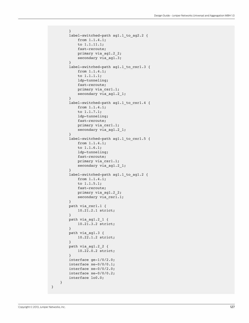
Copyright © 2013, Juniper Networks, Inc. 127
Design Guide - Juniper Networks Universal and Aggregation MBH 1.0
} label-switched-path ag1.1_to_ag2.2 { from 1.1.4.1; to 1.1.11.1; fast-reroute; primary via_ag1.2_2; secondary via_ag1.3; } label-switched-path ag1.1_to_csr1.3 { from 1.1.4.1; to 1.1.1.1; ldp-tunneling; fast-reroute; primary via_csr1.1; secondary via_ag1.2_1; } label-switched-path ag1.1_to_csr1.4 { from 1.1.4.1; to 1.1.7.1; ldp-tunneling; fast-reroute; primary via_csr1.1; secondary via_ag1.2_1; } label-switched-path ag1.1_to_csr1.5 { from 1.1.4.1; to 1.1.6.1; ldp-tunneling; fast-reroute; primary via_csr1.1; secondary via_ag1.2_1; } label-switched-path ag1.1_to_ag1.2 { from 1.1.4.1; to 1.1.5.1; fast-reroute; primary via_ag1.2_2; secondary via_csr1.1; } path via_csr1.1 { 10.21.2.1 strict; } path via_ag1.2_1 { 10.21.3.2 strict; } path via_ag1.3 { 10.22.1.2 strict; } path via_ag1.2_2 { 10.22.0.2 strict; } interface ge-1/0/2.0; interface xe-0/0/0.1; interface xe-0/0/2.0; interface xe-0/0/0.2; interface lo0.0; }}

128 Copyright © 2013, Juniper Networks, Inc.
Design Guide - Juniper Networks Universal and Aggregation MBH 1.0
The following configuration snippet shows the MPLS configuration for Router AG 1.2:
[edit]protocols { rsvp { interface xe-0/0/0.1; interface ge-1/0/2.0; interface xe-0/0/0.2; interface xe-0/0/2.0; } mpls { label-switched-path ag1.2_to_csr1.1 { from 1.1.5.1; to 1.1.3.1; fast-reroute; primary via_csr1.5; secondary via_ag1.2_1; } label-switched-path ag1.2_to_csr1.2 { from 1.1.5.1; to 1.1.2.1; fast-reroute; primary via_csr1.5; secondary via_ag1.2_1; } label-switched-path ag1.2_to_csr1.3 { from 1.1.5.1; to 1.1.1.1; fast-reroute; primary via_csr1.5; secondary via_ag1.2_1; } label-switched-path ag1.2_to_csr1.4 { from 1.1.5.1; to 1.1.7.1; fast-reroute; primary via_csr1.5; secondary via_ag1.2_1; } label-switched-path ag1.2_to_csr1.5 { from 1.1.5.1; to 1.1.6.1; fast-reroute; primary via_csr1.5; secondary via_ag1.2_1; } label-switched-path ag1.2_to_ag2.1 { from 1.1.5.1; to 1.1.10.1; fast-reroute; primary via_ag1.2_2; secondary via_ag1.4; } label-switched-path ag1.2_to_ag2.2 { from 1.1.5.1; to 1.1.11.1; fast-reroute; primary via_ag1.4;
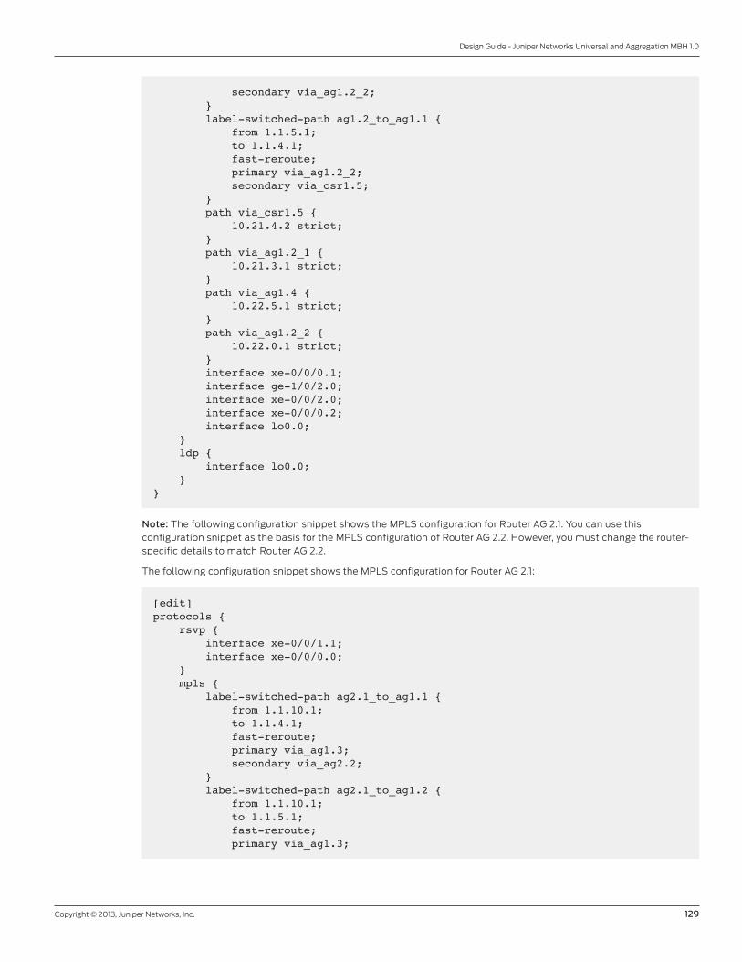
Copyright © 2013, Juniper Networks, Inc. 129
Design Guide - Juniper Networks Universal and Aggregation MBH 1.0
secondary via_ag1.2_2; } label-switched-path ag1.2_to_ag1.1 { from 1.1.5.1; to 1.1.4.1; fast-reroute; primary via_ag1.2_2; secondary via_csr1.5; } path via_csr1.5 { 10.21.4.2 strict; } path via_ag1.2_1 { 10.21.3.1 strict; } path via_ag1.4 { 10.22.5.1 strict; } path via_ag1.2_2 { 10.22.0.1 strict; } interface xe-0/0/0.1; interface ge-1/0/2.0; interface xe-0/0/2.0; interface xe-0/0/0.2; interface lo0.0; } ldp { interface lo0.0; }}
Note: The following configuration snippet shows the MPLS configuration for Router AG 2.1. You can use this
configuration snippet as the basis for the MPLS configuration of Router AG 2.2. However, you must change the router-
specific details to match Router AG 2.2.
The following configuration snippet shows the MPLS configuration for Router AG 2.1:
[edit]protocols { rsvp { interface xe-0/0/1.1; interface xe-0/0/0.0; } mpls { label-switched-path ag2.1_to_ag1.1 { from 1.1.10.1; to 1.1.4.1; fast-reroute; primary via_ag1.3; secondary via_ag2.2; } label-switched-path ag2.1_to_ag1.2 { from 1.1.10.1; to 1.1.5.1; fast-reroute; primary via_ag1.3;

130 Copyright © 2013, Juniper Networks, Inc.
Design Guide - Juniper Networks Universal and Aggregation MBH 1.0
secondary via_ag2.2; } path via_ag2.2 { 10.22.3.2 strict; } path via_ag1.3 { 10.22.2.1 strict; } interface xe-0/0/0.0; interface xe-0/0/1.1; }}
The following configuration snippet shows the routing policy configuration for all routers in the sample network:
[edit}policy-options { policy-statement pplb { then { load-balance per-packet; } }}[...Output truncated...]
[edit]routing-options { forwarding-table { export pplb; }}
To verify the intrasegment MPLS LSP configuration:
1. Verify the status of configured LSPs on each device; issue the show mpls lsp name name ingress detail command.
Specify the name of the LSP for the name option. The ingress option shows the sessions that originate from the router on which the command is run. Check that the following paths and status in the output are up and working as expected:
a. RSVP LSP
b. Primary path
c. Secondary path
d. Standby status
e. Fast reroute status
Configuring Intrasegment OAM (RSVP LSP OAM)
This example illustrates how to configure an RSVP label-switched path (LSP) with OAM on a cell site or aggregation
router to control the status of MPLS LSPs and to track failure events at this level. The BFD protocol is used on each
RSVP LSP. This configuration is based on the topology in Figure 64.
To configure an RSVP LSP with OAM:
• Configure all routers (CSR 1.1 through CSR 1-5, AG 1.1 through AG 1.4, AG 2.1, and AG 2.2) with the BFD protocol on each
RSVP LSP. Set the BFD timer to 100 ms. Note that in an actual network, you might need to tune this timer to fit the BFD
scale. (See the topic “Design Consistency and Scalability Verification.”)
Note: The following configuration snippet shows the RSVP LSP with OAM configurations for Router CSR 1.2. You can
use this configuration snippet as the basis for the RSVP LSP configuration of the following routers—CSR 1.1 through
CSR 1.5, AG 1.1 through AG 1.4, AG 2.1 and AG 2.1. However, you must change the router-specific details to match a
particular CSR , AG 1, and AG 2 router.

Copyright © 2013, Juniper Networks, Inc. 131
Design Guide - Juniper Networks Universal and Aggregation MBH 1.0
The following configuration snippet shows the RSVP LSP with OAM configuration for Router CSR 1.2 to Router AG 1.1:
[edit]protocols { rsvp { interface ge-0/2/1.0; interface ge-0/2/0.0; } mpls { label-switched-path csr1.2_to_ag1.1 { from 1.1.2.1; to 1.1.4.1; fast-reroute; oam { bfd-liveness-detection { minimum-interval 100; multiplier 3; no-adaptation; } } primary via_csr1.1; secondary via_csr1.3; } }}
To verify your RSVP LSP with OAM configuration, issue the show bfd session address and show bfd session detail commands. Specify the loopback address of the BFD peer for the address option. Check the following status and
output fields:
1. Verify that all of the BFD sessions are established and up.
2. Check that the timers negotiated reflect the timers that are configured.
3. Check the BFD statistics.
Configuring Intersegment MPLS Transport
BGP-labeled unicast (BGP-LU) is used to advertise route information between routers in different IGP regions. By
providing connectivity and communication between regions, BPG-LU enables you to massively scale the number of
MPLS-enabled routers on your networks. This example illustrates how to configure MPLS transport on preaggregation
and aggregation routers based on the topology in Figure 65.
For CSRs to resolve the loopback address of the provider edge routers (AG 3.1 and AG 3.2) with a labeled path, you
must configure LDP downstream-on-demand (LDP-DoD; RFC 5036) on the CSRs. The CSR uses LDP-DOD to request
a transport label for every remote provider edge router loopback address. To preserve resiliency at the access region,
LDP-DOD is tunneled over the RSVP LSP. Together, LDP-DOD and BGP-LU establish an end-to-end continuous
labeled-switched (LSP) path from each CSR to each provider edge router. (See Figure 65.)

132 Copyright © 2013, Juniper Networks, Inc.
Design Guide - Juniper Networks Universal and Aggregation MBH 1.0
VLAN 1
VLAN 1
VLAN 2
VLAN 2
ACCESS COREAGGREGATIONPRE-AGGREGATION
CSR 1.3Io0: 1.1.1.1/32
Io0:1.1.3.1/32 Io0:1.1.8.1/32
Io0:1.1.6.1/32 Io0:1.1.9.1/32
AG 1.3
AG 1.4
ge-0/2/0
ge-0/2/110.21.1.1/24
10.21.1.2/24
ge-0/2/0
ge-1/0/210.21.2.1/24
10.21.2.2/24
xe-0/0/2
xe-0/0/210.22.1.1/24
10.22.1.2/24
xe-0/0/0.110.21.3.1/24
xe-0/0/0.110.21.3.2/24
xe-0/0/0.210.22.0.1/24
xe-0/0/0.210.22.0.2/24
ge-0/2/1
ge-1/0/2
10.21.4.2/24
10.21.4.1/24ge-0/2/0
10.21.5.1/24
ge-0/2/010.21.0.1/24
ge-0/2/110.21.0.2/24
ge-0/2/010.21.6.1/24
ge-0/2/110.21.5.2/24
ge-0/2/110.21.6.2/24
xe-0/0/2
xe-0/0/2
10.22.5.2/24
10.22.5.1/24
xe-0/0/0
xe-0/0/010.22.2.1/24
10.22.2.2/24
xe-0/0/110.22.3.1/24
xe-0/0/110.22.3.2/24
xe-0/0/0
xe-0/0/0
10.22.4.2/24
10.22.4.1/24
xe-0/0/2
xe-1/0/210.23.3.1/24
10.23.3.2/24
xe-0/0/2
xe-1/1/310.23.5.1/24
10.23.5.2/24
AS 64501 AS 64502
CSR 1.1
CSR 1.5
Io0:1.1.4.1/32 Io0:1.1.10.1/32Io0:1.1.2.1/32 Io0:1.1.13.1/32
BGP-LU eBGP-LU
Redistribute AG2.x and AG3.x Io0 to inet3
Redistribute CSR Loopbacksto inet3 for BGP-LU Family
RR(RFC 3107)
BFD BFDBGP OAM
LDP-DOD
LDP-DOD LSP BGP-LU LSP
RSVPLSP
CSR 1.2 AG 1.1 AG 2.1 AG 3.1
AG 2.2CSR 1.4 AG 3.2
Io0:1.1.5.1/32Io0:1.1.7.1/32 Io0:1.1.14.1/32Io0:1.1.11.1/32
AG 1.2
10.23.4.1/24
xe-1/0/010.23.4.2/24
RSVPLSP
xe-1/0/0
xe-1/1/110.23.1.2/24
xe-1/1/310.23.2.2/24
xe-0/0/310.23.1.1/24
xe-0/0/310.23.2.1/24
Figure 65: Intersegment MPLS deployment
Configuring BGP-LU
1. To configure an intersegment LSP:
a. Configure IBGP-LU on each AG 1 router to establish BGP peers with Router AG 2.1 and Router AG 2.2.
b. Configure each AG 1 router with an export policy to redistribute the local loopback interface routes into BGP.
c. Configure Router AG 1.1 and Router AG 1.2 with an export policy to redistribute the loopback interface routes from the CSRs into BGP.
d. Configure a RIB group on all AG 1, AG 2, and AG 3 routers to export loopback interface routes from the inet0 routing
table into the inet3 routing table to advertise them as labeled routes using BGP-LU. Use the export policy configured in Step b and Step c to filter routes for export.
2. To configure resiliency and fast failure detection for the BGP-LU session:
a. Configure all AG 1 routers with the BFD protocol for each BGP session; set the BFD timer to 100 ms. Note that in an actual network, you might need to tune this timer to fit the BFD scale. See the topic “Design Consistency and Scalability Verification.”
b. Configure all AG 1 routers with static routes to the loopback (lo0) interface of Router AG 2.1 and Router AG 2.2. As the next hop, use the corresponding RSVP LSP configured in “Configuring Intrasegment MPLS Transport.”
The following configuration snippet shows the BGP-LU configuration for Router AG 1.1; you can use it as the basis for
the BGP-LU configuration of all other AG 1 routers. However, you must change the router-specific details to match a
particular AG 1 router.

Copyright © 2013, Juniper Networks, Inc. 133
Design Guide - Juniper Networks Universal and Aggregation MBH 1.0
[edit]routing-options { rib-groups { inet3-to-inet0 { import-rib [ inet.3 inet.0 ]; } }}policy-options { policy-statement recv-route { term 1 { from { route-filter 1.1.6.1/32 exact; route-filter 1.1.7.1/32 exact; route-filter 1.1.2.1/32 exact; route-filter 1.1.3.1/32 exact; route-filter 1.1.1.1/32 exact; } then reject; } term 2 { then accept; } } policy-statement send-lo0 { term 10 { from { route-filter 1.1.4.1/32 exact; route-filter 1.1.1.1/32 exact; route-filter 1.1.2.1/32 exact; route-filter 1.1.3.1/32 exact; route-filter 1.1.6.1/32 exact; route-filter 1.1.7.1/32 exact; } then accept; } } policy-statement send_inet3_to_inet0 { term 10 { from { route-filter 1.1.0.0/32 address-mask 255.255.0.0; } then accept; } term 20 { then reject; } } policy-statement send_lo0_to_inet3 { term 10 { from { route-filter 1.1.4.1/32 exact; } then accept; } term 20 { then reject; }

134 Copyright © 2013, Juniper Networks, Inc.
Design Guide - Juniper Networks Universal and Aggregation MBH 1.0
}}protocols { bgp { group ag1_ag2_rr { type internal; local-address 1.1.4.1; import recv-route; export send-lo0; bfd-liveness-detection { minimum-interval 100; multiplier 3; no-adaptation; } multipath; neighbor 1.1.10.1 { family inet { labeled-unicast { rib-group inet3-to-inet0; rib { inet.3; } } } } neighbor 1.1.11.1 { family inet { labeled-unicast { rib-group inet3-to-inet0; rib { inet.3; } } } } } }}
The following configuration snippet shows the configuration of static routes for Router AG 1.1; you can use it as the
basis for the static route configuration of all other AG 1 routers. However, you must change the router-specific details to
match a particular AG 1 router.
[edit]routing-options { static { route 1.1.10.1/32 { lsp-next-hop ag1.1_to_ag2.1; } route 1.1.11.1/32 { lsp-next-hop ag1.1_to_ag2.2; } route 1.1.5.1/32 { lsp-next-hop ag1.1_to_ag1.2; } }}

Copyright © 2013, Juniper Networks, Inc. 135
Design Guide - Juniper Networks Universal and Aggregation MBH 1.0
3. Configure IBGP on the AG 2 routers to be peers with the routers in the AG 1 ring:
a. Configure BGP-LU sessions between all AG 2 routers.
b. Configure the AG 2 routers as BGP route reflectors for the routers in the AG 1 ring. Note that the AG 2 routers do not change the next hop for these sessions.
c. Add multipath to the BGP configuration.
4. To configure resiliency and fast failure detection for the BGP-LU session:
a. Configure Router AG 2.1 and Router AG 2.2 with the BFD protocol for each BGP session to the AG 1 routers; set the BFD timer to 100 ms. Note that in an actual network, you might need to tune this timer to fit the BFD scale. See the topic “Design Consistency and Scalability Verification.”
b. Configure Router AG 2.1 and Router AG 2.2 with the BFD protocol for each BGP session to Router AG 2.2 and Router AG 2.1, respectively; set the BFD timer to 10 ms. Note that in an actual network, you might need to tune this timer to fit the BFD scale. See the topic “Design Consistency and Scalability Verification.”
c. Configure Router AG 2.1 and Router AG 2.2 with static routes to the loopback (lo0) interface addresses of the AG 1 routers. As the next hop, use the corresponding RSVP LSP configured in “Configuring Intrasegment MPLS Transport.”
The following configuration snippet shows the configuration of IBGP and BGP-LU (Step 3 and Step 4) on Router AG 2.1;
you can use this configuration as the basis for the IBGP and BGP-LU configuration on Router AG 2.2. However, you must
change the router-specific details to match Router AG 2.2.
[edit]routing-options { interface-routes { rib-group inet inet0-to-inet3; } rib-groups { inet3-to-inet0 { import-rib [ inet.3 inet.0 ]; } inet0-to-inet3 { import-rib [ inet.0 inet.3 ]; import-policy rib_import; } }}protocols { bgp { group ag2_ibgp { type internal; local-address 1.1.10.1; bfd-liveness-detection { minimum-interval 10; multiplier 3; no-adaptation; } multipath; neighbor 1.1.11.1 { family inet { labeled-unicast { rib-group inet3-to-inet0; rib { inet.3; } } } } } group ag1_rr {
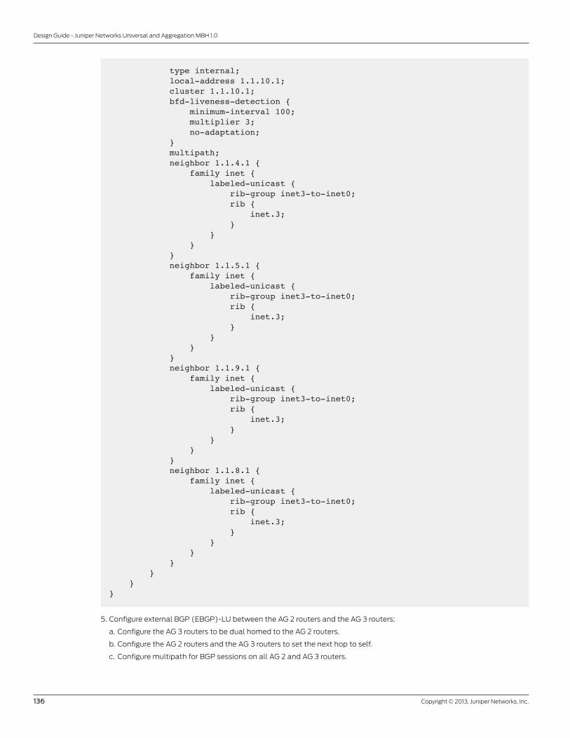
136 Copyright © 2013, Juniper Networks, Inc.
Design Guide - Juniper Networks Universal and Aggregation MBH 1.0
type internal; local-address 1.1.10.1; cluster 1.1.10.1; bfd-liveness-detection { minimum-interval 100; multiplier 3; no-adaptation; } multipath; neighbor 1.1.4.1 { family inet { labeled-unicast { rib-group inet3-to-inet0; rib { inet.3; } } } } neighbor 1.1.5.1 { family inet { labeled-unicast { rib-group inet3-to-inet0; rib { inet.3; } } } } neighbor 1.1.9.1 { family inet { labeled-unicast { rib-group inet3-to-inet0; rib { inet.3; } } } } neighbor 1.1.8.1 { family inet { labeled-unicast { rib-group inet3-to-inet0; rib { inet.3; } } } } } }}
5. Configure external BGP (EBGP)-LU between the AG 2 routers and the AG 3 routers:
a. Configure the AG 3 routers to be dual homed to the AG 2 routers.
b. Configure the AG 2 routers and the AG 3 routers to set the next hop to self.
c. Configure multipath for BGP sessions on all AG 2 and AG 3 routers.

Copyright © 2013, Juniper Networks, Inc. 137
Design Guide - Juniper Networks Universal and Aggregation MBH 1.0
6. Configure resiliency and fast failure detection for the BGP-LU session on the AG 2 and the AG 3 routers:
a. Configure Router AG 2.1, Router AG 2.2, Router AG 3.1, and Router AG 3.2 with the BFD protocol for each EBGP session; set the BFD timer to 10 ms. Note that in an actual network, you might need to tune this timer to fit the BFD scale. See the topic “Design Consistency and Scalability Verification.”
The following configuration snippet shows the configuration of routing policy and EBGP-LU on Router AG 2.1; you can
use the configuration as the basis for the routing policy and EBGP-LU configuration on Router AG 2.2. However, you
must change the router-specific details to match Router AG 2.2.
[edit]policy-options { policy-statement adv_lb { term local { from { protocol direct; route-filter 1.1.10.1/32 exact; } then accept; } term ag1-ring { from { route-filter 1.1.4.1/32 exact; route-filter 1.1.5.1/32 exact; route-filter 1.1.9.1/32 exact; route-filter 1.1.8.1/32 exact; } then accept; } }}protocols { bgp { group ebgp { type external; export adv_lb; peer-as 64502; bfd-liveness-detection { minimum-interval 100; multiplier 3; no-adaptation; } multipath; neighbor 10.23.1.2 { local-address 10.23.1.1; family inet { labeled-unicast { rib-group inet3-to-inet0; per-prefix-label; rib { inet.3; } } } } neighbor 10.23.3.2 { local-address 10.23.3.1; family inet { labeled-unicast { rib-group inet3-to-inet0;

138 Copyright © 2013, Juniper Networks, Inc.
Design Guide - Juniper Networks Universal and Aggregation MBH 1.0
per-prefix-label; rib { inet.3; } } } } } }}
The following configuration snippet shows the configuration of routing policy and EBGP-LU on Router AG 3.1; you can
use the configuration as the basis for the routing policy and EBGP-LU configuration for Router AG 3.2. However, you
must change the router-specific details to match Router AG 3.2.
[edit]routing-options { interface-routes { rib-group inet inet0-to-inet3; } rib-groups { inet3-to-inet0 { import-rib [ inet.3 inet.0 ]; } inet0-to-inet3 { import-rib [ inet.0 inet.3 ]; import-policy rib_import; } }}policy-options { policy-statement adv_lb { term local { from { protocol direct; route-filter 1.1.13.1/32 exact; } then accept; } term rej_all { then reject; } } policy-statement metric_rem { term 1 { from protocol bgp; then { metric { minimum-igp; } accept; } } }}

Copyright © 2013, Juniper Networks, Inc. 139
Design Guide - Juniper Networks Universal and Aggregation MBH 1.0
protocols { bgp { group ebgp { type external; export adv_lb; peer-as 64501; bfd-liveness-detection { minimum-interval 100; multiplier 3; no-adaptation; } multipath; neighbor 10.23.3.1 { local-address 10.23.3.2; family inet { labeled-unicast { rib-group inet3-to-inet0; rib { inet.3; } } } } neighbor 10.23.2.1 { local-address 10.23.2.2; family inet { labeled-unicast { rib-group inet3-to-inet0; rib { inet.3; } } } } } group ag3_ibgp { type internal; local-address 1.1.13.1; export adv_lb; bfd-liveness-detection { minimum-interval 10; multiplier 3; no-adaptation; } neighbor 1.1.14.1 { family inet { labeled-unicast { rib-group inet3-to-inet0; rib { inet.3; } } } } } }}
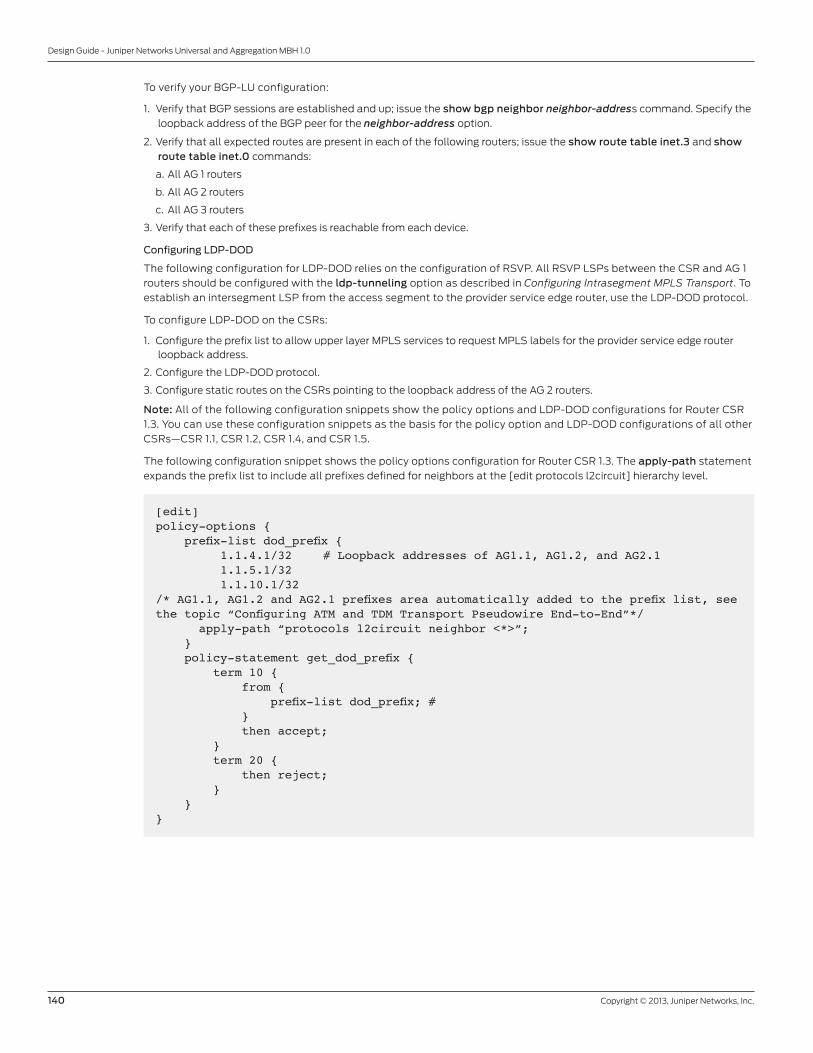
140 Copyright © 2013, Juniper Networks, Inc.
Design Guide - Juniper Networks Universal and Aggregation MBH 1.0
To verify your BGP-LU configuration:
1. Verify that BGP sessions are established and up; issue the show bgp neighbor neighbor-address command. Specify the
loopback address of the BGP peer for the neighbor-address option.
2. Verify that all expected routes are present in each of the following routers; issue the show route table inet.3 and show route table inet.0 commands:
a. All AG 1 routers
b. All AG 2 routers
c. All AG 3 routers
3. Verify that each of these prefixes is reachable from each device.
Configuring LDP-DOD
The following configuration for LDP-DOD relies on the configuration of RSVP. All RSVP LSPs between the CSR and AG 1
routers should be configured with the ldp-tunneling option as described in Configuring Intrasegment MPLS Transport. To
establish an intersegment LSP from the access segment to the provider service edge router, use the LDP-DOD protocol.
To configure LDP-DOD on the CSRs:
1. Configure the prefix list to allow upper layer MPLS services to request MPLS labels for the provider service edge router loopback address.
2. Configure the LDP-DOD protocol.
3. Configure static routes on the CSRs pointing to the loopback address of the AG 2 routers.
Note: All of the following configuration snippets show the policy options and LDP-DOD configurations for Router CSR
1.3. You can use these configuration snippets as the basis for the policy option and LDP-DOD configurations of all other
CSRs—CSR 1.1, CSR 1.2, CSR 1.4, and CSR 1.5.
The following configuration snippet shows the policy options configuration for Router CSR 1.3. The apply-path statement
expands the prefix list to include all prefixes defined for neighbors at the [edit protocols l2circuit] hierarchy level.
[edit]policy-options { prefix-list dod_prefix { 1.1.4.1/32 # Loopback addresses of AG1.1, AG1.2, and AG2.1 1.1.5.1/32 1.1.10.1/32/* AG1.1, AG1.2 and AG2.1 prefixes area automatically added to the prefix list, see the topic “Configuring ATM and TDM Transport Pseudowire End-to-End”*/ apply-path “protocols l2circuit neighbor <*>”; } policy-statement get_dod_prefix { term 10 { from { prefix-list dod_prefix; # } then accept; } term 20 { then reject; } }}
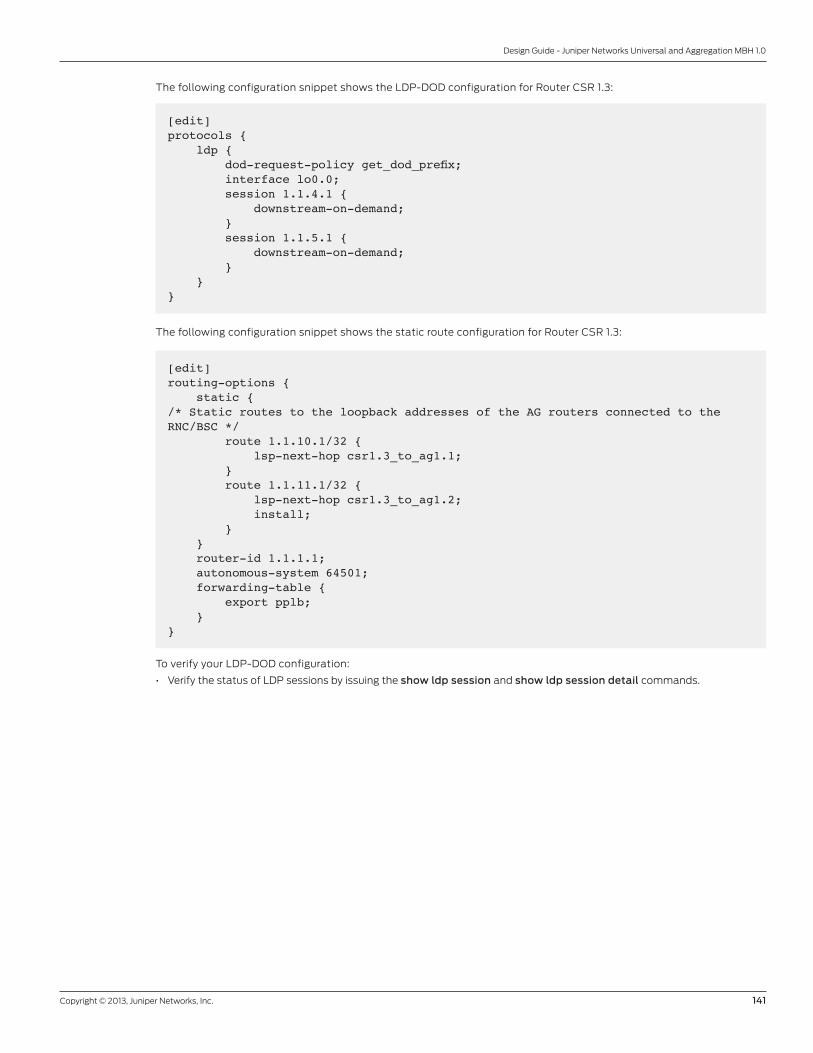
Copyright © 2013, Juniper Networks, Inc. 141
Design Guide - Juniper Networks Universal and Aggregation MBH 1.0
The following configuration snippet shows the LDP-DOD configuration for Router CSR 1.3:
[edit]protocols { ldp { dod-request-policy get_dod_prefix; interface lo0.0; session 1.1.4.1 { downstream-on-demand; } session 1.1.5.1 { downstream-on-demand; } }}
The following configuration snippet shows the static route configuration for Router CSR 1.3:
[edit]routing-options { static {/* Static routes to the loopback addresses of the AG routers connected to the RNC/BSC */ route 1.1.10.1/32 { lsp-next-hop csr1.3_to_ag1.1; } route 1.1.11.1/32 { lsp-next-hop csr1.3_to_ag1.2; install; } } router-id 1.1.1.1; autonomous-system 64501; forwarding-table { export pplb; }}
To verify your LDP-DOD configuration:
• Verify the status of LDP sessions by issuing the show ldp session and show ldp session detail commands.

142 Copyright © 2013, Juniper Networks, Inc.
Design Guide - Juniper Networks Universal and Aggregation MBH 1.0
Configuring End-to-End Layer 3 VPN ServicesA Layer 3 VPN is a set of sites that share common routing information and whose connectivity is controlled by a
collection of policies. This deployment scenario illustrates how to configure a Layer 3 VPN using Multiprotocol internal
BGP (MP-IBGP) and Multiprotocol external BGP (MP-EBGP) to distribute VPN routes across the CSR access ring and
across different autonomous systems. The configuration is based on the network topology in Figure 66 and Figure 67,
and can be used across the following service profiles—4G LTE and HSPA.
At a high level, to establish an end-to-end Layer 3 VPN, you need to:
1. Configure MP-BGP in the network to signal MPLS labels for the Layer 3 VPN service and to distribute VRF routes. (See Figure 66 and the topic “Configuring MP-BGP.”)
2. Configure a routing instance for the Layer 3 VPN and UNI interfaces at each service router—CSR 1.1 through CSR 1.5, AG 1.1, AG 1.2, AG 3.1 and AG 3.2. (See Figure 67 and the topic “Configuring the Routing Instance for the Layer 3 VPN.”)
ACCESS COREAGGREGATIONPRE-AGGREGATION
CSR 1.3Io0: 1.1.1.1/32
Io0:1.1.8.1/32
Io0:1.1.9.1/32
AG 1.3
AG 1.4
ge-0/2/0
ge-0/2/110.21.1.1/24
10.21.1.2/24
ge-0/2/0
ge-1/0/210.21.2.1/24
10.21.2.2/24
xe-0/0/2
xe-0/0/210.22.1.1/24
10.22.1.2/24
VLAN 1
VLAN 1
xe-0/0/0.110.21.3.1/24
xe-0/0/0.110.21.3.2/24
VLAN 2
VLAN 2
xe-0/0/0.210.22.0.1/24
xe-0/0/0.210.22.0.2/24
ge-0/2/1
ge-1/0/2
10.21.4.2/24
10.21.4.1/24ge-0/2/0
10.21.5.1/24
ge-0/2/010.21.0.1/24
ge-0/2/110.21.0.2/24
ge-0/2/010.21.6.1/24
ge-0/2/110.21.5.2/24
ge-0/2/110.21.6.2/24
xe-0/0/2
xe-0/0/2
10.22.5.2/24
10.22.5.1/24
xe-0/0/0
xe-0/0/010.22.2.1/24
10.22.2.2/24
xe-0/0/110.22.3.1/24
xe-0/0/110.22.3.2/24
xe-0/0/0
xe-0/0/0
10.22.4.2/24
10.22.4.1/24
xe-0/0/2
xe-1/0/210.23.3.1/24
10.23.3.2/24
xe-0/0/2
xe-1/1/3
10.23.5.1/24
10.23.5.2/24
AS 64501 AS 64502
Io0:1.1.10.1/32Io0:1.1.2.1/32 Io0:1.1.13.1/32
AG 1.1 AG 2.1 AG 3.1
AG 2.2CSR 1.4 AG 3.2
Io0:1.1.5.1/32Io0:1.1.7.1/32 Io0:1.1.14.1/32Io0:1.1.11.1/32
RR(RFC 3107)
MP-EBGP (Option C)
BFDBGP OAM
MP-BGP
BFD
Default
NHS
Io0:1.1.6.1/32
CSR 1.2
Io0:1.1.3.1/32
CSR 1.1
Io0:1.1.4.1/32
CSR 1.5 AG 1.2
10.23.4.1/24
xe-1/0/010.23.4.2/24
xe-1/0/0
xe-0/0/310.23.1.1/24
xe-1/1/110.23.1.2/24
xe-0/0/310.23.2.1/24
xe-1/1/310.23.2.2/24
Figure 66: MP-BGP deployment for Layer 3 VPN services
The network in Figure 66 has the following characteristics:
1. BGP in the CSR access ring:
a. Each CSR has an MP-IBGP session (family inet-vpn unicast) to each AG 1 router in the access ring.
b. BGP multipath is enabled for each session.
c. Per packet load balancing is enabled on all CSRs.
d. Each AG 1 router has an MP-IBGP session to each CSR in the access ring.
e. AG 1 routers act as route reflectors for all the CSRs in the access ring.
f. An MP-IBGP session is established between all the AG 1 routers.
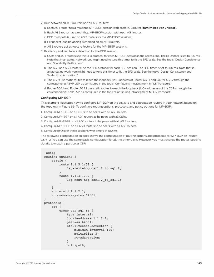
Copyright © 2013, Juniper Networks, Inc. 143
Design Guide - Juniper Networks Universal and Aggregation MBH 1.0
2. BGP between all AG 3 routers and all AG 1 routers:
a. Each AG 1 router has a multihop MP-EBGP session with each AG 3 router (family inet-vpn unicast).
b. Each AG 3 router has a multihop MP-EBGP session with each AG 1 router.
c. BGP multipath is used on AG 3 routers for the MP-EBGP sessions.
d. Per packet load balancing is enabled on all AG 3 routers.
e. AG 3 routers act as route reflectors for the MP-EBGP sessions.
3. Resiliency and fast failure detection for the BGP session:
a. CSRs and AG 1 routers use the BFD protocol for each MP-BGP session in the access ring. The BFD timer is set to 100 ms. Note that in an actual network, you might need to tune this timer to fit the BFD scale. See the topic “Design Consistency and Scalability Verification.”
b. The AG 1 and AG 3 routers use the BFD protocol for each BGP session. The BFD timer is set to 100 ms. Note that in an actual network, you might need to tune this timer to fit the BFD scale. See the topic “Design Consistency and Scalability Verification.”
c. The CSRs use static routes to reach the loopback (lo0) address of Router AG 1.1 and Router AG 1.2 through the corresponding RSVP LSP, as configured in the topic “Configuring Intrasegment MPLS Transport.”
d. Router AG 1.1 and Router AG 1.2 use static routes to reach the loopback (lo0) addresses of the CSRs through the corresponding RSVP LSP, as configured in the topic “Configuring Intrasegment MPLS Transport.”
Configuring MP-BGP
This example illustrates how to configure MP-BGP on the cell site and aggregation routers in your network based on
the topology in Figure 66. To configure routing options, protocols, and policy options for MP-BGP:
1. Configure MP-IBGP on all CSRs to be peers with all AG 1 routers.
2. Configure MP-IBGP on all AG 1 routers to be peers with all CSRs.
3. Configure MP-EBGP on all AG 1 routers to be peers with all AG 3 routers.
4. Configure MP-EBGP on all AG 3 routers to be peers with all AG 1 routers.
5. Configure BFD over these sessions with timers of 100 ms.
The following configuration snippet shows the configuration of routing options and protocols for MP-BGP on Router
CSR 1.2. You can use the same basic configuration for all the other CSRs. However, you must change the router-specific
details to match a particular CSR.
[edit]routing-options { static { route 1.1.5.1/32 { lsp-next-hop csr1.2_to_ag1.2; } route 1.1.4.1/32 { lsp-next-hop csr1.2_to_ag1.1; } } router-id 1.1.2.1; autonomous-system 64501;}protocols { bgp { group csr_ag1_rr { type internal; local-address 1.1.2.1; peer-as 64501; bfd-liveness-detection { minimum-interval 100; multiplier 3; no-adaptation; } multipath;

144 Copyright © 2013, Juniper Networks, Inc.
Design Guide - Juniper Networks Universal and Aggregation MBH 1.0
neighbor 1.1.4.1 { family inet-vpn { unicast; } } neighbor 1.1.5.1 { family inet-vpn { unicast; } } } }}
The following configuration snippet shows the configuration of routing options, protocols, and policy options for
MP-IBGP on Router AG 1.1. You can use the same basic configuration for all the other AG 1 routers. However, you must
change the router-specific details to match a particular AG 1 router.
[edit]routing-options { static { route 1.1.3.1/32 { lsp-next-hop ag1.1_to_csr1.1; } route 1.1.2.1/32 { lsp-next-hop ag1.1_to_csr1.2; } route 1.1.1.1/32 { lsp-next-hop ag1.1_to_csr1.3; } route 1.1.7.1/32 { lsp-next-hop ag1.1_to_csr1.4; } route 1.1.6.1/32 { lsp-next-hop ag1.1_to_csr1.5; } } router-id 1.1.4.1; autonomous-system 64501;}protocols { bgp { group csr_ag1_rr { type internal; local-address 1.1.4.1; family inet-vpn { unicast; } export [ NHS summarize ]; cluster 1.1.4.1; peer-as 64501; bfd-liveness-detection { minimum-interval 100; multiplier 3; no-adaptation; } multipath;

Copyright © 2013, Juniper Networks, Inc. 145
Design Guide - Juniper Networks Universal and Aggregation MBH 1.0
neighbor 1.1.1.1; neighbor 1.1.2.1; neighbor 1.1.3.1; neighbor 1.1.6.1; neighbor 1.1.7.1; } } }policy-options { policy-statement NHS { term 10 { then { next-hop self; } } } policy-statement summarize { term 1 { from { route-filter 192.0.0.0/13 exact; } then accept; } term 2 { from { route-filter 192.0.0.0/13 orlonger reject; } } }}
The following configuration snippet shows the MP-EBGP configuration on Router AG 1.1. You can use the same basic
configuration for all the other AG 1 routers. However, you must change the router-specific details, such as the bgp
local-address, to match a particular AG 1 router.
[edit]protocols { bgp { group option_c_for_l3vpn { type external; local-address 1.1.4.1; peer-as 64502; bfd-liveness-detection { minimum-interval 100; multiplier 3; no-adaptation; } multipath; neighbor 1.1.13.1 { multihop { ttl 64; } family inet-vpn { unicast; } } neighbor 1.1.14.1 {

146 Copyright © 2013, Juniper Networks, Inc.
Design Guide - Juniper Networks Universal and Aggregation MBH 1.0
multihop { ttl 64; } family inet-vpn { unicast; } } } }}
The following configuration snippet shows the configuration of MP-EBGP for Router AG 3.1. You can use the same basic
configuration for all the other AG 3 routers. However, you must change the router-specific details, such as the bgp
local-address, to match a particular AG 3 router.
[edit]protocols { bgp { group option_c_for_l3vpn { type external; bfd-liveness-detection { minimum-interval 100; multiplier 3; no-adaptation; } neighbor 1.1.4.1 { multihop { ttl 64; } local-address 1.1.13.1; family inet-vpn { unicast; } peer-as 64501; } neighbor 1.1.5.1 { multihop { ttl 64; } local-address 1.1.13.1; family inet-vpn { unicast; } peer-as 64501; } } }}
To verify your BGP and BFD setup:
1. Verify that the BGP sessions are established; issue the show bgp neighbor neighbor-address command and check that
the BFD sessions are up. Specify the loopback-address of the neighbor for the neighbor-address option.
2. Verify that the static routes are installed and have precedence over IS-IS routes; use the show route terse command.
3. From each router, use the ping host command to check that the ping takes the LSP path. Specify the loopback address
of the remote routers for the host option.
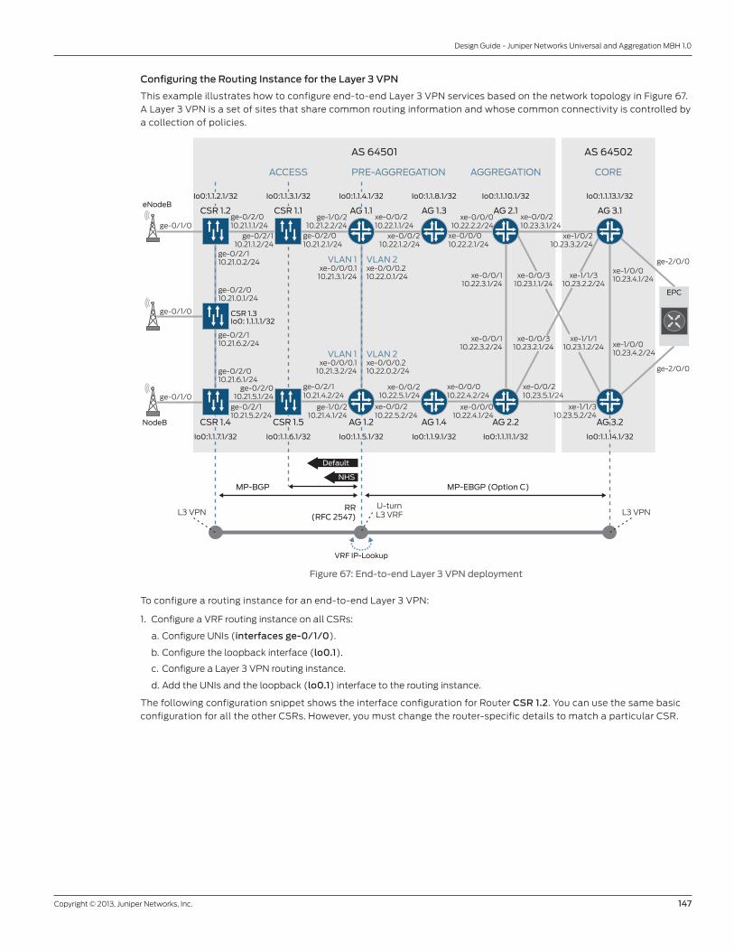
Copyright © 2013, Juniper Networks, Inc. 147
Design Guide - Juniper Networks Universal and Aggregation MBH 1.0
Configuring the Routing Instance for the Layer 3 VPN
This example illustrates how to configure end-to-end Layer 3 VPN services based on the network topology in Figure 67.
A Layer 3 VPN is a set of sites that share common routing information and whose common connectivity is controlled by
a collection of policies.
ACCESS COREAGGREGATIONPRE-AGGREGATION
AS 64501 AS 64502
EPC
ge-0/1/0
ge-0/1/0
ge-0/1/0
ge-2/0/0
ge-2/0/0
RR(RFC 2547)
CSR 1.3Io0: 1.1.1.1/32
AG 1.3AG 1.1 AG 2.1
AG 1.4 AG 2.2AG 1.2
CSR 1.2
CSR 1.4
AG 3.1
NodeB
eNodeB
AG 3.2
CSR 1.1
CSR 1.5
MP-EBGP (Option C)
ge-0/2/010.21.1.1/24
ge-0/2/110.21.1.2/24
ge-0/2/010.21.2.1/24
ge-1/0/210.21.2.2/24
xe-0/0/210.22.1.1/24
xe-0/0/210.22.1.2/24
VLAN 1
VLAN 1
xe-0/0/0.110.21.3.1/24
xe-0/0/0.110.21.3.2/24
VLAN 2
VLAN 2
xe-0/0/0.210.22.0.1/24
xe-0/0/0.210.22.0.2/24
ge-0/2/110.21.4.2/24
ge-1/0/210.21.4.1/24
ge-0/2/010.21.5.1/24
ge-0/2/010.21.0.1/24
ge-0/2/110.21.0.2/24
ge-0/2/010.21.6.1/24
ge-0/2/110.21.5.2/24
ge-0/2/110.21.6.2/24
xe-0/0/210.22.5.2/24
xe-0/0/210.22.5.1/24
xe-0/0/010.22.2.1/24
xe-0/0/010.22.2.2/24
xe-0/0/010.22.4.2/24
xe-0/0/010.22.4.1/24
xe-0/0/210.23.3.1/24
xe-1/0/210.23.3.2/24
xe-0/0/210.23.5.1/24
xe-1/1/310.23.5.2/24
MP-BGP
Default
NHS
Io0:1.1.4.1/32 Io0:1.1.10.1/32Io0:1.1.8.1/32 Io0:1.1.13.1/32Io0:1.1.2.1/32 Io0:1.1.3.1/32
Io0:1.1.5.1/32 Io0:1.1.11.1/32Io0:1.1.7.1/32 Io0:1.1.9.1/32 Io0:1.1.14.1/32Io0:1.1.6.1/32
10.23.4.1/24
xe-1/0/010.23.4.2/24
xe-1/0/0
VRF IP-Lookup
L3 VPNL3 VPNU-turnL3 VRF
xe-0/0/110.22.3.1/24
xe-0/0/110.22.3.2/24
xe-1/1/110.23.1.2/24
xe-1/1/310.23.2.2/24
xe-0/0/310.23.1.1/24
xe-0/0/310.23.2.1/24
Figure 67: End-to-end Layer 3 VPN deployment
To configure a routing instance for an end-to-end Layer 3 VPN:
1. Configure a VRF routing instance on all CSRs:
a. Configure UNIs (interfaces ge-0/1/0).
b. Configure the loopback interface (lo0.1).
c. Configure a Layer 3 VPN routing instance.
d. Add the UNIs and the loopback (lo0.1) interface to the routing instance.
The following configuration snippet shows the interface configuration for Router CSR 1.2. You can use the same basic
configuration for all the other CSRs. However, you must change the router-specific details to match a particular CSR.

148 Copyright © 2013, Juniper Networks, Inc.
Design Guide - Juniper Networks Universal and Aggregation MBH 1.0
The following configuration snippet shows the VLAN configuration on an Ethernet interface on Router CSR 1.2:
[edit]interfaces { ge-0/1/0 { vlan-tagging; encapsulation flexible-ethernet-services; unit 0 { vlan-id 1; family inet { address 183.1.1.1/24; } } unit 1 { vlan-id 2; family inet { address 183.1.2.1/24; } } unit 2 { vlan-id 3; family inet { address 183.1.3.1/24; } } } lo0 { unit 1 { family inet { address 1.1.2.100/32; } } }}
The following configuration snippet shows the routing instance configuration for Router CSR 1.2:
[edit]routing-instances { csr_l3vpn { instance-type vrf; interface ge-0/1/0.0; interface ge-0/1/0.1; interface ge-0/1/0.2; interface lo0.1; route-distinguisher 100:1; vrf-target target:100:1; vrf-table-label; }}
2. Configure all the AG 1 routers with a routing instance (previously referred to as a U-turn VRF ):
a. Configure the loopback interface (lo0.1).
b. Configure a Layer 3 routing instance.
c. Add the loopback (lo0.1) interface to the routing instance.
d. Configure the routing instance with the vrf-table-label statement.

Copyright © 2013, Juniper Networks, Inc. 149
Design Guide - Juniper Networks Universal and Aggregation MBH 1.0
The following configuration snippet shows the routing instance configuration for Router AG 1.1. You can use the same
basic configuration for all the other AG 1 routers. However, you must change the router-specific details, such as
loopback lo0.1 family inet address, to match a particular AG 1 router.
[edit]interfaces { lo0 { unit 1 { family inet { address 1.1.4.100/32; } } }}
[edit]routing-instances { csr_l3vpn { instance-type vrf; interface lo0.1; route-distinguisher 100:1; vrf-target target:100:1; vrf-table-label; }}
3. Configure all AG 3 routers with a routing instance:
a. Configure UNIs (interfaces ge-2/0/0).
b. Configure the loopback interface (lo0.1).
c. Configure a Layer 3 VPN routing instance.
d. Add the loopback interface lo0.1.
e. Add UNIs.
The following configuration snippet shows the interface configuration for Router AG 3.1. You can use the same basic
configuration for all the other AG 3 routers. However, you must change the router-specific details to match a particular
AG 3 router.
[edit]interfaces { ge-2/0/0 { vlan-tagging; encapsulation flexible-ethernet-services; unit 0 { vlan-id 1; family inet { address 113.1.1.1/24; } } unit 1 { vlan-id 2; family inet { address 113.1.2.1/24; } } unit 2 { vlan-id 3; family inet {

150 Copyright © 2013, Juniper Networks, Inc.
Design Guide - Juniper Networks Universal and Aggregation MBH 1.0
address 113.1.3.1/24; } } } lo0 { unit 1 { family inet { address 1.1.13.100/32; } } }}
The following configuration snippet shows the routing instance configuration for Router AG 3.1. You can use the same
basic configuration for all the other AG 3 routers. However, you must change the router-specific details to match a
particular AG 3 router.
[edit]routing-instances { l3vpn { instance-type vrf; interface ge-2/0/0.0; interface ge-2/0/0.1; interface ge-2/0/0.2; interface lo0.1; route-distinguisher 100:1; vrf-target target:100:1; vrf-table-label; routing-options { multipath { vpn-unequal-cost equal-external-internal; } } }}
To verify your Layer 3 VPN configuration:
• On AG 1, AG 2, and AG 3 routers, issue the show route table l3vpn.inet.0 extensive command, and check the
following routes:
a. Verify that the routes advertised from all CSRs are learnt on all AG 3 routers.
b. Verify that the routes are load-balanced according to multipath.
c. Verify that there are no VPNv4 routes on any AG 2 routers.
d. Verify that AG 1 routers receive only a summary route from AG 3 routers.
e. Verify that AG 1 routers receive all the routes from AG 1 routers.
• On CRS routers, issue the show route table csr_l3vpn.inet.0 extensive command, and check the following routes:
a. Verify that all CSRs receive only a summary route.
b. Verify the label stack at each CSR.
c. Verify the number of routes and labels at each CSR.

Copyright © 2013, Juniper Networks, Inc. 151
Design Guide - Juniper Networks Universal and Aggregation MBH 1.0
Configuring Layer 2 VPN to Layer 3 VPN Termination ServicesThis deployment scenario illustrates how to configure a Layer 3 VPN in conjunction with a Layer 2 pseudowire in the
access segment. There are various reasons to use Layer 2 pseudowire in the access segment and to stitch together
Layer 2 services with Layer 3 services on preaggregation routers (AG 1 in this sample network topology). For example, it
simplifies configuration on CSRs.
The configuration is based on the network topology in Figure 68 and Figure 69, which you can use for the HSPA service
profile and for the 4G LTE service profile.
VRRP Master
Iub IP
Iub IPIub IP
NodeB
RNC
3GACCESS PRE-AGGREGATION
AGGREGATION
AG 1.2
CSR 1.n
AG 1.1 AG 3.1
AG 3.2
MP-EBGP
ge-0/1/0
Logical Tunnel (lt) Interface
L3 VPNL2 VPN
Trac FlowConnection at the Service Level
Active PseudowireBackup Pseudowire (not in hot standby)
MP-EBGP
Figure 68: Layer 2 VPN to Layer 3 VPN termination
Figure 68 shows traffic flowing from the NodeB tower to the RNC over a pseudowire, MP-EBGP, and a Layer 3 VPN,
providing an end-to-end service. A backup pseudowire provides redundancy.
The network in Figure 68 has the following characteristics:
• Layer 2 pseudowires in the access segment between CSR and AG 1 routers (see the topic “Configuring Layer 2
Pseudowires in the Access Segment”):
- Each CSR has multiple Ethernet and VLAN pseudowires dual homed to AG 1 routers.
- Active and standby pseudowires are terminated on the AG 1.1 router and the AG 1.2 router, respectively.
- Each pseudowire uses a Gigabit Ethernet interface on CSRs and a logical tunnel (lt) interface on AG 1 routers as
pseudowire endpoints.
• Inter-AS Layer 3 VPNs on all AG 1 and AG 3 routers (see the topic “Configuring Inter-AS Layer 3 VPN”):
- MB-EBGP is used to signal an MPLS label for the Layer 3 VPN service and to distribute VRF routes between AG 1 and
AG 3 routes across different autonomous systems.
- A VRF instance is created on all AG 1 routers. This instance includes the loopback interface.
- A VRF instance is created on all AG 3 routers. This instance includes the UNI and loopback interface.
• A Layer 2 pseudowire to Layer 3 VPN termination on all AG 1 routers (see the topic “Configuring a Layer 2 Pseudowire to
Layer 3 VPN Termination”:
- Each AG 1 router has pseudowires (multiple) to each CSR with a logical tunnel (lt) interface at the pseudowire end.
- Pseudowires are terminated into a VRF routing instance at each AG 1 router by including the corresponding logical
tunnel interfaces to the VRF instance.
- A VRRP instance is used for virtual IPv4 addressing assignment to the logical tunnel interfaces in the VRF routing instance.
- A VRF instance is created on all AG 1 routers with the loopback interface (lo0) and the logical tunnel interfaces.

152 Copyright © 2013, Juniper Networks, Inc.
Design Guide - Juniper Networks Universal and Aggregation MBH 1.0
Configuring Layer 2 Pseudowires in the Access Segment
This example illustrates how to configure a pseudowire and Layer 3 VPN based on the network topology in Figure 69.
The following service-level configuration relies on the configuration of intrasegment and intersegment MPLS transport
described in the topics “Configuring Intrasegment MPLS Transport” and “Configuring Intersegment MPLS Transport.”
ACCESS COREAGGREGATIONPRE-AGGREGATION
AS 64501 AS 64502
RNC
ge-0/1/0
ge-0/1/0
ge-0/1/0
ge-2/0/0
ge-2/0/0
CSR 1.3Io0: 1.1.1.1/32
AG 1.4 AG 2.2NodeB
eNodeB
ge-0/2/010.21.1.1/24
ge-0/2/110.21.1.2/24
ge-0/2/010.21.2.1/24
ge-1/0/210.21.2.2/24
xe-0/0/210.22.1.1/24
xe-0/0/210.22.1.2/24
VLAN 1
VLAN 1
xe-0/0/0.110.21.3.1/24
xe-0/0/0.110.21.3.2/24
VLAN 2
VLAN 2
xe-0/0/0.210.22.0.1/24
xe-0/0/0.210.22.0.2/24
ge-0/2/110.21.4.2/24
ge-1/0/210.21.4.1/24
ge-0/2/010.21.5.1/24
ge-0/2/010.21.0.1/24
ge-0/2/110.21.0.2/24
ge-0/2/010.21.6.1/24
ge-0/2/110.21.5.2/24
ge-0/2/110.21.6.2/24
xe-0/0/210.22.5.2/24
xe-0/0/210.22.5.1/24
xe-0/0/010.22.2.1/24
xe-0/0/010.22.2.2/24
xe-0/0/010.22.4.2/24
xe-0/0/010.22.4.1/24
xe-0/0/210.23.3.1/24
xe-1/0/210.23.3.2/24
xe-0/0/210.23.5.1/24
xe-1/1/310.23.5.2/24
Io0:1.1.10.1/32Io0:1.1.8.1/32 Io0:1.1.13.1/32
Io0:1.1.11.1/32Io0:1.1.9.1/32
10.23.4.1/24
xe-1/0/010.23.4.2/24
xe-1/0/0
MP-EBGP (Option C)T-LDPT-LDP
Logical Tunnel (lt) InterfacePseudowire Termination in L3 VRF
AG 1.3 AG 2.1 AG 3.1
AG 1.2CSR 1.4 CSR 1.5
Io0:1.1.5.1/32Io0:1.1.7.1/32 Io0:1.1.6.1/32
Io0:1.1.4.1/32Io0:1.1.2.1/32 Io0:1.1.3.1/32
AG 1.1CSR 1.2 CSR 1.1
IS-IS Level 2
VRRP Groups
IS-IS Level 1
AG 3.2
Io0:1.1.14.1/32
L3VPNL3 VPNPseudowire
xe-0/0/110.22.3.1/24
xe-0/0/110.22.3.2/24
xe-0/0/310.23.1.1/24
xe-1/1/310.23.2.2/24
xe-1/1/110.23.1.2/24
xe-0/0/310.23.2.1/24
Figure 69: Deployment scenario of Layer 2 VPN to Layer 3 VPN termination
To configure a pseudowire and Layer 3 VPN based on the network in Figure 69:
1. Configure all CSRs with Layer 2 pseudowires to Router AG 1.1 and Router AG 1.2:
a. Configure UNIs with which to originate the Layer 2 VPN.
b. Configure a Layer 2 pseudowire from each CSR to Router AG 1.1 and Router AG 1.2 by using targeted LDP (T-LDP) signaling.
c. Configure active and backup pseudowires to add redundancy.
Note: Do not enable hot standby because it does not work correctly with pseudowire to Layer 3 termination.

Copyright © 2013, Juniper Networks, Inc. 153
Design Guide - Juniper Networks Universal and Aggregation MBH 1.0
The following configuration snippet shows the interface configuration for Router CSR 1.2. You can use these
configuration snippets as the basis for the interface and Layer 2 protocol configurations of all other CSRs—CSR 1.1, CSR
1.3, CSR 1.4, and CSR 1.5. However, you must change the router-specific details to match a particular CSR:
[edit]interfaces { ge-0/1/0 { flexible-vlan-tagging; encapsulation flexible-ethernet-services; unit 10 { encapsulation vlan-ccc; vlan-id 20; family ccc; } unit 11 { encapsulation vlan-ccc; vlan-id 21; family ccc; }[...Output truncated...] unit 19 { encapsulation vlan-ccc; vlan-id 29; family ccc; } }
The following configuration snippet shows the Layer 2 configuration for Router CSR 1.2:
[edit]protocols { l2circuit { neighbor 1.1.4.1 { interface ge-0/1/0.10 { virtual-circuit-id 20; backup-neighbor 1.1.5.1; } interface ge-0/1/0.11 { virtual-circuit-id 21; backup-neighbor 1.1.5.1; } interface ge-0/1/0.12 { virtual-circuit-id 22; backup-neighbor 1.1.5.1; } interface ge-0/1/0.13 { virtual-circuit-id 23; backup-neighbor 1.1.5.1; } interface ge-0/1/0.14 { virtual-circuit-id 24; backup-neighbor 1.1.5.1; } interface ge-0/1/0.15 { virtual-circuit-id 25; backup-neighbor 1.1.5.1; }
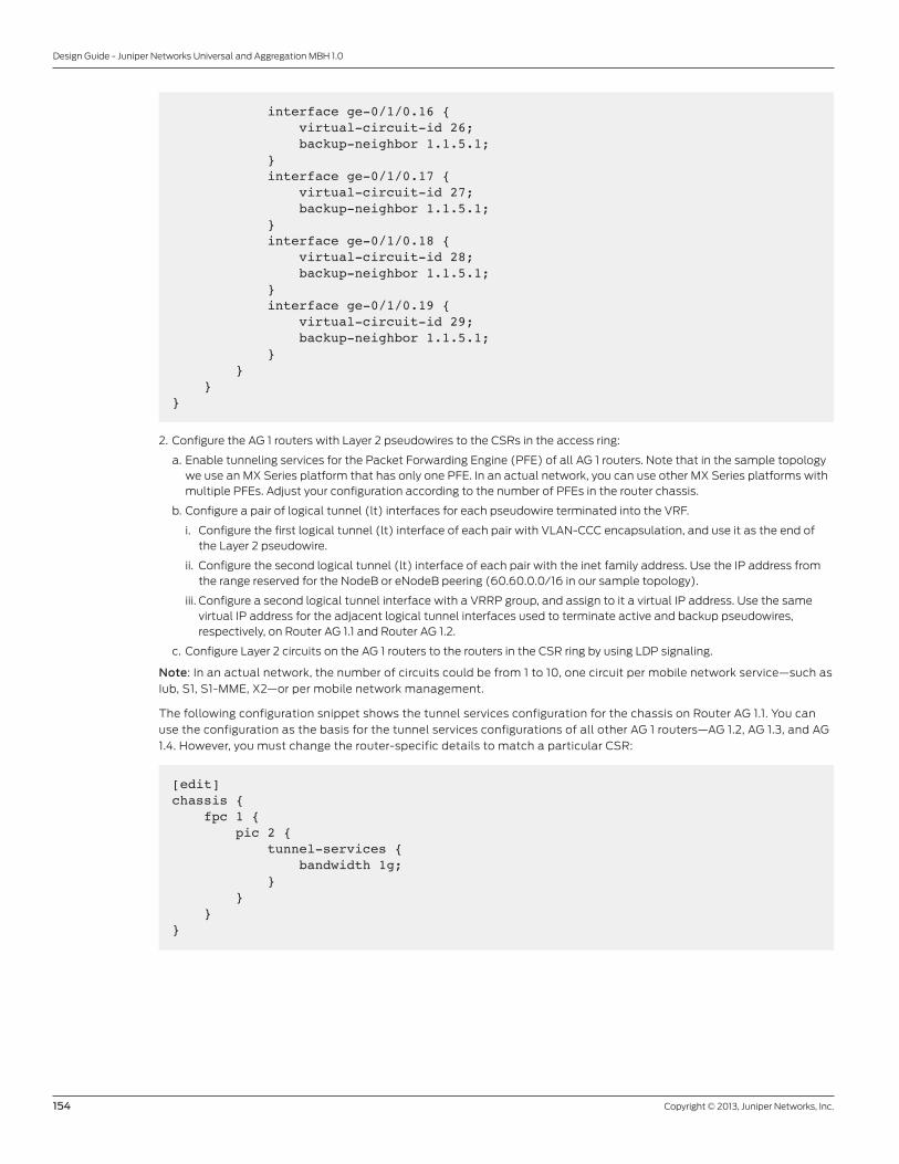
154 Copyright © 2013, Juniper Networks, Inc.
Design Guide - Juniper Networks Universal and Aggregation MBH 1.0
interface ge-0/1/0.16 { virtual-circuit-id 26; backup-neighbor 1.1.5.1; } interface ge-0/1/0.17 { virtual-circuit-id 27; backup-neighbor 1.1.5.1; } interface ge-0/1/0.18 { virtual-circuit-id 28; backup-neighbor 1.1.5.1; } interface ge-0/1/0.19 { virtual-circuit-id 29; backup-neighbor 1.1.5.1; } } }}
2. Configure the AG 1 routers with Layer 2 pseudowires to the CSRs in the access ring:
a. Enable tunneling services for the Packet Forwarding Engine (PFE) of all AG 1 routers. Note that in the sample topology we use an MX Series platform that has only one PFE. In an actual network, you can use other MX Series platforms with multiple PFEs. Adjust your configuration according to the number of PFEs in the router chassis.
b. Configure a pair of logical tunnel (lt) interfaces for each pseudowire terminated into the VRF.
i. Configure the first logical tunnel (lt) interface of each pair with VLAN-CCC encapsulation, and use it as the end of the Layer 2 pseudowire.
ii. Configure the second logical tunnel (lt) interface of each pair with the inet family address. Use the IP address from the range reserved for the NodeB or eNodeB peering (60.60.0.0/16 in our sample topology).
iii. Configure a second logical tunnel interface with a VRRP group, and assign to it a virtual IP address. Use the same virtual IP address for the adjacent logical tunnel interfaces used to terminate active and backup pseudowires, respectively, on Router AG 1.1 and Router AG 1.2.
c. Configure Layer 2 circuits on the AG 1 routers to the routers in the CSR ring by using LDP signaling.
Note: In an actual network, the number of circuits could be from 1 to 10, one circuit per mobile network service—such as
Iub, S1, S1-MME, X2—or per mobile network management.
The following configuration snippet shows the tunnel services configuration for the chassis on Router AG 1.1. You can
use the configuration as the basis for the tunnel services configurations of all other AG 1 routers—AG 1.2, AG 1.3, and AG
1.4. However, you must change the router-specific details to match a particular CSR:
[edit]chassis { fpc 1 { pic 2 { tunnel-services { bandwidth 1g; } } }}

Copyright © 2013, Juniper Networks, Inc. 155
Design Guide - Juniper Networks Universal and Aggregation MBH 1.0
The following configuration snippet shows the logical tunnel interface configuration for Router AG 1.1. You can use
the same basic configuration for all the other AG 1 routers. However, you must change the router-specific details (like
family inet address) to match a particular AG 1 router:
interfaces { lt-1/2/10 { logical-tunnel-options { per-unit-mac-disable; } unit 10 { encapsulation vlan-ccc; vlan-id 10; peer-unit 11; family ccc; } unit 11 { encapsulation vlan; vlan-id 10; peer-unit 10; family inet { address 60.60.1.1/24 { vrrp-group 10 { virtual-address 60.60.1.10; } } } } unit 12 { encapsulation vlan-ccc; vlan-id 11; peer-unit 13; family ccc; } unit 13 { encapsulation vlan; vlan-id 11; peer-unit 12; family inet { address 60.60.2.1/24 { vrrp-group 11 { virtual-address 60.60.2.10; } } } }[...Output truncated...] # Circuits to CRS1.1 skipped for brevity unit 108 { encapsulation vlan-ccc; vlan-id 59; peer-unit 109; family ccc; } unit 109 { encapsulation vlan; vlan-id 59; peer-unit 108; family inet { address 60.60.50.1/24 {

156 Copyright © 2013, Juniper Networks, Inc.
Design Guide - Juniper Networks Universal and Aggregation MBH 1.0
vrrp-group 59 { virtual-address 60.60.50.10; } } } } }}
The following configuration snippet shows the Layer 2 circuit configuration for Router AG 1.1 and Router AG 1.2:
[edit]protocols { l2circuit { neighbor 1.1.1.1 { [...Output truncated...] # Circuits to CRS1.1 were skipped for brevity } neighbor 1.1.2.1 { # Circuits to CSR1.2 interface lt-1/2/10.30 { virtual-circuit-id 20; } interface lt-1/2/10.32 { virtual-circuit-id 21; } interface lt-1/2/10.34 { virtual-circuit-id 22; } interface lt-1/2/10.36 { virtual-circuit-id 23; } interface lt-1/2/10.38 { virtual-circuit-id 24; } interface lt-1/2/10.40 { virtual-circuit-id 25; } interface lt-1/2/10.42 { virtual-circuit-id 26; } interface lt-1/2/10.44 { virtual-circuit-id 27; } interface lt-1/2/10.46 { virtual-circuit-id 28; } interface lt-1/2/10.48 { virtual-circuit-id 29; } } [...Output truncated...] # Four neighbors skipped for brevity neighbor 1.1.7.1 { interface lt-1/2/10.90 { virtual-circuit-id 50; } interface lt-1/2/10.92 { virtual-circuit-id 51; }
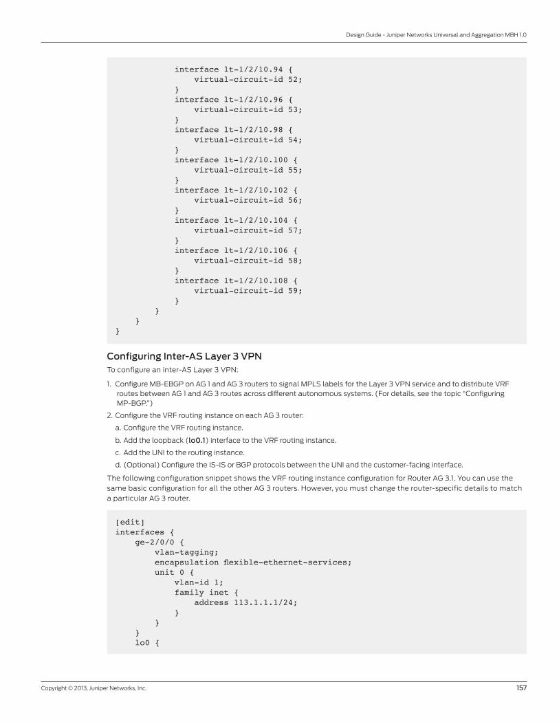
Copyright © 2013, Juniper Networks, Inc. 157
Design Guide - Juniper Networks Universal and Aggregation MBH 1.0
interface lt-1/2/10.94 { virtual-circuit-id 52; } interface lt-1/2/10.96 { virtual-circuit-id 53; } interface lt-1/2/10.98 { virtual-circuit-id 54; } interface lt-1/2/10.100 { virtual-circuit-id 55; } interface lt-1/2/10.102 { virtual-circuit-id 56; } interface lt-1/2/10.104 { virtual-circuit-id 57; } interface lt-1/2/10.106 { virtual-circuit-id 58; } interface lt-1/2/10.108 { virtual-circuit-id 59; } } }}
Configuring Inter-AS Layer 3 VPN To configure an inter-AS Layer 3 VPN:
1. Configure MB-EBGP on AG 1 and AG 3 routers to signal MPLS labels for the Layer 3 VPN service and to distribute VRF routes between AG 1 and AG 3 routes across different autonomous systems. (For details, see the topic “Configuring MP-BGP.”)
2. Configure the VRF routing instance on each AG 3 router:
a. Configure the VRF routing instance.
b. Add the loopback (lo0.1) interface to the VRF routing instance.
c. Add the UNI to the routing instance.
d. (Optional) Configure the IS-IS or BGP protocols between the UNI and the customer-facing interface.
The following configuration snippet shows the VRF routing instance configuration for Router AG 3.1. You can use the
same basic configuration for all the other AG 3 routers. However, you must change the router-specific details to match
a particular AG 3 router.
[edit]interfaces { ge-2/0/0 { vlan-tagging; encapsulation flexible-ethernet-services; unit 0 { vlan-id 1; family inet { address 113.1.1.1/24; } } } lo0 {

158 Copyright © 2013, Juniper Networks, Inc.
Design Guide - Juniper Networks Universal and Aggregation MBH 1.0
unit 1 { family inet { address 1.1.13.100/32; } } }}
[edit]routing-instances { csr_l3vpn { instance-type vrf; interface ge-2/0/0.0; interface lo0.1; route-distinguisher 200:200; vrf-target target:200:200; routing-options { static { route 1.1.100.100/32 next-hop 26.0.0.2; } router-id 1.1.13.100; autonomous-system 64502; } protocols { bgp { group vpn { type external; local-address 26.0.0.1; peer-as 65003; local-as 64502; neighbor 26.0.0.2; } } } }}
Configuring a Layer 2 Pseudowire to Layer 3 VPN Termination
To configure a Layer 2 pseudowire to terminate at a Layer 3 VPN:
1. Configure the VRF routing instance on each AG 1 router to the routers in the CSR ring:
a. Configure the VRF routing instance.
b. Add loopback interface (lo0.1) to the VRF routing instance.
c. Add the logical tunnel (lt) interfaces (Layer 3 peers) to the routing instance.
The following configuration snippet shows the routing instance configuration for Router AG 1.1. You can use the same
basic configuration for all the other AG 1 routers. However, you must change the router-specific details to match a
particular AG 1 router.
[edit]policy-options { policy-statement vpn1-export { term 20 { from protocol direct; then { metric add 100; community add vpn4;

Copyright © 2013, Juniper Networks, Inc. 159
Design Guide - Juniper Networks Universal and Aggregation MBH 1.0
community add from_ibgp; accept; } } } community from_ibgp members target:200:2001; community vpn4 members target:200:200;} routing-instances { csr_l3vpn { instance-type vrf; interface lt-1/2/10.11; [...Output truncated...] interface lt-1/2/10.29; interface lt-1/2/10.31; interface lt-1/2/10.33; interface lt-1/2/10.35; interface lt-1/2/10.37; interface lt-1/2/10.39; [...Output truncated...] interface lt-1/2/10.127; interface lt-1/2/10.129; interface lo0.1; route-distinguisher 200:200; vrf-export vpn1-export; vrf-target target:200:200; vrf-table-label; }}
To verify your pseudowire and Layer 3 VPN setup:
1. Verify that all pseudowires are established:
a. On all CSR and AG 1 routers, issue the show l2circuit connection command.
2. On AG 1 and AG 3 routers, issue the show route table csr_13vpn.inet3 command to verify the following routes:
a. Check that the csr_l3vpn routing instance advertises all the routes learned from the CSRs to the AG 3 routers.
b. Check that the csr_l3vpn routing instance receives all the routes from all the AG 1 routers.
c. Check that the csr_l3vpn routing instance advertises only a default or aggregate route towards all the AG 1 routers.

160 Copyright © 2013, Juniper Networks, Inc.
Design Guide - Juniper Networks Universal and Aggregation MBH 1.0
Configuring a Layer 2 VPN to VPLS Termination ServiceA Layer 2 VPN forwards packets in a point-to-point fashion only. For VPLS traffic, packets can traverse the network in
a point-to-multipoint fashion, meaning that a packet originating from a customer edge router can broadcast to all the
provider edge routers participating in the VPLS routing instance. The packet traverses the service provider’s network
over an MPLS label-switched path (LSP), allowing you to connect geographically dispersed Ethernet LAN sites to each
other across an MPLS backbone. The paths carrying VPLS traffic between each PE router participating in a routing
instance are called pseudowires. The next sample configuration is based on the network topology in Figure 70 and
Figure 71, which you can use for the HSPA and 4G LTE service profiles.
IubEthernet
IubEthernet
NodeB
RNC
3GIP/MPLSACCESS
PRE-AGGREGATION
AGGREGATION
AG 1.2
CSR 1.n
AG 1.1 AG 3.1
VPLS Hub
Iub Ethernet
AG 3.2
T-LDP
T-LDP
VPLSL2 VPN
Tra�c FlowConnection at the Service Level
Active PseudowireBackup Pseudowire (Standby)
Figure 70: Layer 2 VPN to VPLS termination
Figure 70 shows traffic flowing from the tower to the RNC over a pseudowire in the IP/MPLS access network, across
a unicast targeted LDP (T-LDP) session, and a VPLS routing instance, providing an end-to-end service. A backup
pseudowire provides redundancy. The network in Figure 70 has the following characteristics:
1. A pseudowire on all CSRs in the access segment. See the topic “Configuring a Pseudowire in the Access Segment (VPLS Spoke)”:
• Each router in the CSR ring has multiple Ethernet or VLAN pseudowires to the dual homed AG 1 routers.
• Each pseudowire has an active and standby termination on Router AG 1.1 and Router AG 1.2.
• The pseudowire status type, length, variable (TLV) feature is enabled for all pseudowires. The pseudowire TLV is used to
communicate the status of a pseudowire back and forth between CSR and AG 1 routers.
2. A VPLS hub in the preaggregation segment on all AG 1 routers. See the topic “Configuring a VPLS Hub in the Preaggregation Segment”:
• Each AG 1 router has multiple pseudowires to each router in the CSR ring.
• The status TLV is enabled on these pseudowires.
• Mesh groups are used to map the pseudowire to the VPLS instance.
3. An end-to-end inter-AS with AG 1 and AG 3 routers as VPLS service nodes. See the topic “Configuring End-to-End Inter-Autonomous System VPLS.”
4. A VPLS routing instance configured on all AG 3 routers that receive all the pseudowire TLV mapping messages sent from all the AG 1 routers.
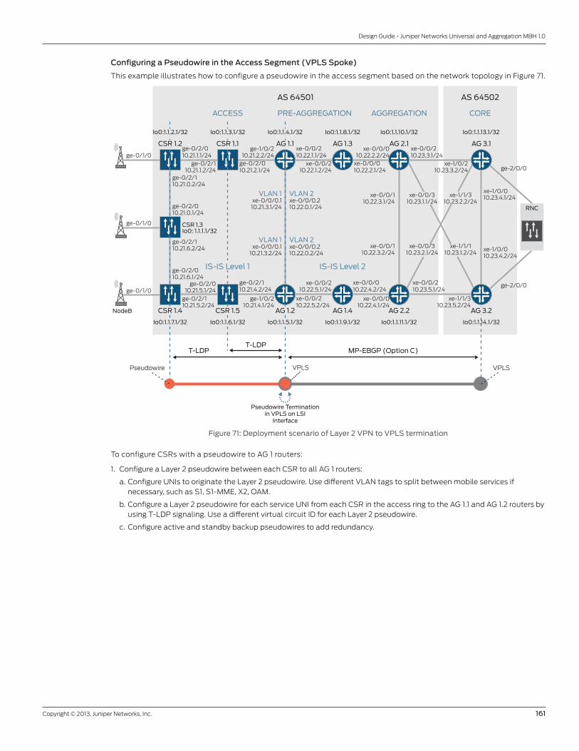
Copyright © 2013, Juniper Networks, Inc. 161
Design Guide - Juniper Networks Universal and Aggregation MBH 1.0
Configuring a Pseudowire in the Access Segment (VPLS Spoke)
This example illustrates how to configure a pseudowire in the access segment based on the network topology in Figure 71.
ACCESS COREAGGREGATIONPRE-AGGREGATION
AS 64501 AS 64502
RNC
ge-0/1/0
ge-0/1/0
ge-0/1/0
ge-2/0/0
ge-2/0/0
CSR 1.3Io0: 1.1.1.1/32
AG 1.4 AG 2.2NodeB
ge-0/2/010.21.1.1/24
ge-0/2/110.21.1.2/24
ge-0/2/010.21.2.1/24
ge-1/0/210.21.2.2/24
xe-0/0/210.22.1.1/24
xe-0/0/210.22.1.2/24
VLAN 1
VLAN 1
xe-0/0/0.110.21.3.1/24
xe-0/0/0.110.21.3.2/24
VLAN 2
VLAN 2
xe-0/0/0.210.22.0.1/24
xe-0/0/0.210.22.0.2/24
ge-0/2/110.21.4.2/24
ge-1/0/210.21.4.1/24
ge-0/2/010.21.5.1/24
ge-0/2/010.21.0.1/24
ge-0/2/110.21.0.2/24
ge-0/2/010.21.6.1/24
ge-0/2/110.21.5.2/24
ge-0/2/110.21.6.2/24
xe-0/0/210.22.5.2/24
xe-0/0/210.22.5.1/24
xe-0/0/010.22.2.1/24
xe-0/0/010.22.2.2/24
xe-0/0/010.22.4.2/24
xe-0/0/010.22.4.1/24
xe-0/0/210.23.3.1/24
xe-1/0/210.23.3.2/24
xe-0/0/210.23.5.1/24
xe-1/1/310.23.5.2/24
Io0:1.1.10.1/32Io0:1.1.8.1/32 Io0:1.1.13.1/32
Io0:1.1.11.1/32Io0:1.1.9.1/32 Io0:1.1.14.1/32
10.23.4.1/24
xe-1/0/010.23.4.2/24
xe-1/0/0
MP-EBGP (Option C)T-LDPT-LDP
AG 1.3 AG 2.1 AG 3.1
AG 1.2CSR 1.4 CSR 1.5
Io0:1.1.5.1/32Io0:1.1.7.1/32 Io0:1.1.6.1/32
Io0:1.1.4.1/32Io0:1.1.2.1/32 Io0:1.1.3.1/32
AG 1.1CSR 1.2 CSR 1.1
IS-IS Level 2IS-IS Level 1
AG 3.2
Pseudowire Terminationin VPLS on LSI
Interface
VPLS VPLSPseudowire
xe-0/0/110.22.3.1/24
xe-0/0/110.22.3.2/24
xe-1/1/110.23.1.2/24
xe-1/1/310.23.2.2/24
xe-0/0/310.23.1.1/24
xe-0/0/310.23.2.1/24
Figure 71: Deployment scenario of Layer 2 VPN to VPLS termination
To configure CSRs with a pseudowire to AG 1 routers:
1. Configure a Layer 2 pseudowire between each CSR to all AG 1 routers:
a. Configure UNIs to originate the Layer 2 pseudowire. Use different VLAN tags to split between mobile services if necessary, such as S1, S1-MME, X2, OAM.
b. Configure a Layer 2 pseudowire for each service UNI from each CSR in the access ring to the AG 1.1 and AG 1.2 routers by using T-LDP signaling. Use a different virtual circuit ID for each Layer 2 pseudowire.
c. Configure active and standby backup pseudowires to add redundancy.

162 Copyright © 2013, Juniper Networks, Inc.
Design Guide - Juniper Networks Universal and Aggregation MBH 1.0
The following configuration snippet shows the interface configuration for Router CSR 1.1. You can use this snippet as
the basis for the interface configuration of all other routers in the CSR ring. However, you must change the router-
specific details to match a particular CSR.
[edit]interfaces { ge-0/1/0 { vlan-tagging; encapsulation flexible-ethernet-services; unit 0 { encapsulation vlan-ccc; vlan-id 1; } unit 1 { encapsulation vlan-ccc; vlan-id 2; } unit 2 { encapsulation vlan-ccc; vlan-id 3; } }}
The following configuration snippet shows the Layer 2 pseudowire configuration for Router CSR 1.1. You can use this
configuration as the basis for the protocol configuration of all other CSRs. However, you must change the router-
specific details to match a particular CSR.
[edit]protocols { l2circuit { neighbor 1.1.4.1 { interface ge-0/1/0.0 { virtual-circuit-id 12; pseudowire-status-tlv; backup-neighbor 1.1.5.1 { virtual-circuit-id 13; standby; } } interface ge-0/1/0.1 { virtual-circuit-id 22; pseudowire-status-tlv; backup-neighbor 1.1.5.1 { virtual-circuit-id 23; standby; } } interface ge-0/1/0.2 { virtual-circuit-id 32; pseudowire-status-tlv; backup-neighbor 1.1.5.1 { virtual-circuit-id 33; standby; } } } }}

Copyright © 2013, Juniper Networks, Inc. 163
Design Guide - Juniper Networks Universal and Aggregation MBH 1.0
Configuring a VPLS Hub in the Preaggregation Segment
To configure a VPLS hub in the preaggregation segment:
1. Configure a VPLS hub on all AG 1 routers:
a. Configure a VPLS routing instance on the AG 1.1 router and the AG 1.2 router.
b. Configure VPLS routing instance peers to span across the following routers: AG 1.1, AG 1.2, AG 3.1, and AG 3.2.
c. Configure mesh groups within the VPLS instance for each mobile network service (such as Iub, S1, S1-MME, and X2) with the routers in the CSR ring as VPLS spokes. Use the same VPLS ID for each mesh group as you did for the
corresponding virtual-circuit-id in the Layer 2 VPNs on the VPLS spokes (CSRs). For details, see the topic “Configuring a Pseudowire in the Access Segment (VPLS Spoke).”
d. Add the local-switching statement, which allows you to terminate multiple Layer 2 circuit pseudowires at a single VPLS mesh group (essential for X2 connectivity).
The following configuration snippet shows the dynamic profiles and VPLS routing instance (virtual-switch)
configuration for Router AG 1.1. You can use this configuration as the basis for the routing instance configuration of all
other AG 1 routers. However, you must change the router-specific details to match a particular AG 1 router.
[edit]dynamic-profiles { data_profile { interfaces { “$junos-interface-ifd-name” { unit “$junos-underlying-interface-unit” { family bridge { interface-mode trunk; vlan-id-list 12; } } } } } oam_profile { interfaces { “$junos-interface-ifd-name” { unit “$junos-underlying-interface-unit” { family bridge { interface-mode trunk; vlan-id-list 22; } } } } } extra_profile { interfaces { “$junos-interface-ifd-name” { unit “$junos-underlying-interface-unit” { family bridge { interface-mode trunk; vlan-id-list 32; } } } } }}routing-instances { vs_1 {

164 Copyright © 2013, Juniper Networks, Inc.
Design Guide - Juniper Networks Universal and Aggregation MBH 1.0
instance-type virtual-switch; protocols { vpls { no-tunnel-services; vpls-id 4514; mac-flush; neighbor 1.1.5.1; neighbor 1.1.14.1; neighbor 1.1.13.1; mesh-group data_pw { vpls-id 12; local-switching; neighbor 1.1.1.1 { associate-profile data_profile; encapsulation-type ethernet-vlan; no-vlan-id-validate; } neighbor 1.1.2.1 { associate-profile data_profile; encapsulation-type ethernet-vlan; no-vlan-id-validate; } neighbor 1.1.7.1 { associate-profile data_profile; encapsulation-type ethernet-vlan; no-vlan-id-validate; } neighbor 1.1.6.1 { associate-profile data_profile; encapsulation-type ethernet-vlan; no-vlan-id-validate; } neighbor 1.1.3.1 { associate-profile data_profile; encapsulation-type ethernet-vlan; no-vlan-id-validate; } } mesh-group extra_pw { vpls-id 32; local-switching; neighbor 1.1.1.1 { associate-profile extra_profile; encapsulation-type ethernet-vlan; no-vlan-id-validate; } neighbor 1.1.2.1 { associate-profile extra_profile; encapsulation-type ethernet-vlan; no-vlan-id-validate; } neighbor 1.1.7.1 { associate-profile extra_profile; encapsulation-type ethernet-vlan; no-vlan-id-validate; } neighbor 1.1.6.1 { associate-profile extra_profile;

Copyright © 2013, Juniper Networks, Inc. 165
Design Guide - Juniper Networks Universal and Aggregation MBH 1.0
encapsulation-type ethernet-vlan; no-vlan-id-validate; } neighbor 1.1.3.1 { associate-profile extra_profile; encapsulation-type ethernet-vlan; no-vlan-id-validate; } } mesh-group oam_pw { vpls-id 22; local-switching; neighbor 1.1.1.1 { associate-profile oam_profile; encapsulation-type ethernet-vlan; no-vlan-id-validate; } neighbor 1.1.2.1 { associate-profile oam_profile; encapsulation-type ethernet-vlan; no-vlan-id-validate; } neighbor 1.1.7.1 { associate-profile oam_profile; encapsulation-type ethernet-vlan; no-vlan-id-validate; } neighbor 1.1.6.1 { associate-profile oam_profile; encapsulation-type ethernet-vlan; no-vlan-id-validate; } neighbor 1.1.3.1 { associate-profile oam_profile; encapsulation-type ethernet-vlan; no-vlan-id-validate; } } } } bridge-domains { data_vlan { domain-type bridge; vlan-id 1; } extra_vlan { domain-type bridge; vlan-id 3; } oam_vlan { domain-type bridge; vlan-id 2; } } }}

166 Copyright © 2013, Juniper Networks, Inc.
Design Guide - Juniper Networks Universal and Aggregation MBH 1.0
Configuring End-to-End Inter-Autonomous System VPLS
To configure end-to-end inter-AS VPLS:
1. Configure VPLS on all the AG 3 routers:
a. Configure a VPLS instance on Router AG 3.1 and Router AG 3.2.
b. Configure VPLS instance peers to span across the following routers—AG 1.1, AG 1.2, AG 3.1, and AG 3.2. Use the same VPLS ID as for the VPLS instance on the AG 1.1 and AG 1.2 routers.
The following configuration snippet shows the configuration of VLAN encapsulation and ID of interfaces for Router AG
3.1. You can use this configuration as the basis for the VLAN encapsulation and ID configuration for Router AG 3.2.
[edit]interfaces { ge-2/0/0 { flexible-vlan-tagging; encapsulation flexible-ethernet-services; unit 0 { encapsulation vlan-vpls; vlan-id 1; } unit 1 { encapsulation vlan-vpls; vlan-id 2; } }}
The following configuration snippet shows the configuration of LDP for Router AG 3.1. You can use the configuration as
the basis for configuring Router AG 3.2.
protocols { ldp { interface lo0.0; }}
The following configuration snippet shows the configuration of a VPLS routing instance for Router AG 3.1. You can use
the configuration as the basis for the VPLS routing instance configuration for Router AG 3.2.
routing-instances { vpls_1 { instance-type vpls; vlan-id all; interface ge-2/0/0.0; interface ge-2/0/0.1; protocols { vpls { no-tunnel-services; mac-flush; mesh-group ag1_spoke { vpls-id 4514; neighbor 1.1.4.1; neighbor 1.1.5.1; neighbor 1.1.14.1; } } } }}

Copyright © 2013, Juniper Networks, Inc. 167
Design Guide - Juniper Networks Universal and Aggregation MBH 1.0
Configuring ATM Pseudowire and SAToP/CESoPSN ServicesAn Asynchronous Transfer Mode (ATM) pseudowire acts as a Layer 2 circuit or service, which allows the migration of
ATM services to an MPLS packet-switched network without having to provision the ATM subscriber or customer edge
device. Structure-Agnostic time-division multiplexing (TDM) over Packet (SAToP), as defined in RFC 4553, Structure-
Agnostic TDM over Packet (SAToP), is used for pseudowire encapsulation for TDM bits (T1, E1). The encapsulation
disregards any structure imposed on the T1 and E1 streams, in particular the structure imposed by standard TDM
framing. Circuit Emulation Service over Packet-Switched Network (CESoPSN) is a method of encapsulating TDM
signals into CESoPSN packets, and in the reverse direction, de-encapsulating CESoPSN packets back into TDM signals.
This configuration is based on the network topology in Figure 72, and can be used for the 3G and 2G service profiles.
AS 64501
ACCESS PRE-AGGREGATION AGGREGATION
ds-0/0/3:1
CSR 1.3
AG 1.4
RNC/BSC
Io0: 1.1.1.1/32
Io0:1.1.3.1/32 Io0:1.1.8.1/32
Io0:1.1.6.1/32 Io0:1.1.9.1/32
AG 1.3AG 1.1 AG 2.1
AG 2.2AG 1.2
ds-0/0/0:1e1-0/0/1
e1-0/0/10
ge-0/2/0
ge-0/2/110.21.1.1/24
10.21.1.2/24ge-0/2/010.21.2.1/24
ge-1/0/210.21.2.2/24
xe-0/0/2
xe-0/0/210.22.1.1/24
10.22.1.2/24
ds-1/2/5:1 at-1/2/0e1-1/2/10e1-1/2/6
ds-1/2/0:1e1-1/2/10e1-1/2/1
xe-0/0/210.22.0.1/24
xe-0/0/110.21.3.1/24
xe-0/0/210.22.0.2/24
xe-0/0/110.21.3.2/24
ge-0/2/110.21.4.2/24
ge-1/0/210.21.4.1/24
ge-0/2/010.21.5.1/24
ge-0/2/010.21.0.1/24
ge-0/2/110.21.0.2/24
ge-0/2/010.21.6.1/24
ge-0/2/110.21.5.2/24
ge-0/2/110.21.6.2/24
e1-0/0/1e1-0/0/10 xe-0/0/2
10.22.5.2/24
xe-0/0/210.22.5.1/24
xe-0/0/010.22.2.1/24
xe-0/0/010.22.2.2/24
xe-0/0/010.22.4.2/24
xe-0/0/010.22.4.1/24
at-0/0/16
T-LDP(For ATM Pseudowire Signaling)
T-LDP (For TDM Pseudowire)
CSR 1.2 CSR 1.1
CSR 1.4 CSR 1.5
TDM Pseudowire
Io0:1.1.4.1/32 Io0:1.1.10.1/32Io0:1.1.2.1/32
Io0:1.1.5.1/32 Io0:1.1.11.1/32Io0:1.1.7.1/32
ATMATM
ATM PW3
CESoPSN/SAToP
CESoPSN/SAToP
xe-0/0/110.22.3.1/24
xe-0/0/110.22.3.2/24
Figure 72: Deployment of SAToP and CESoPSN
Figure 72 shows virtual ATM (at) interfaces, channelized (ds) interfaces, and E1 (e1) interfaces connecting the RAN with
the CSRs CSR 1.3 and CSR 1.4. The following configuration relies on configuration of intrasegment and intersegment
MPLS transport, as shown in the topics “Configuring Intrasegment MPLS Transport” and “Configuring Intersegment
MPLS Transport.”
Configuring ATM and TDM Transport Pseudowire End-to-End
To configure an ATM and TDM pseudowire on Router CSR 1.3 and Router CSR 1.4:
1. Configure the physical properties of the channelized E1 (ce1) interfaces, and define the NxDS0 and E1 interfaces used for TDM circuit emulation services.
2. Configure the encapsulation type for DS0 and E1 interfaces (cesopsn or satop).
3. Configure inverse multiplexing for ATM (IMA) on Router CSR 1.3 and Router CSR 1.4.
4. Configure pseudowire Layer 2 circuits for each ds0, e1, and virtual ATM (at) interface.

168 Copyright © 2013, Juniper Networks, Inc.
Design Guide - Juniper Networks Universal and Aggregation MBH 1.0
The following configuration snippet shows the chassis and interfaces configuration for Router CSR 1.3. You can use
the configuration as the basis for the routing instance configuration of Router CSR 1.4. However, you must change the
router-specific details to match Router CSR 1.4.
[edit]chassis { fpc 0 { pic 0 { framing e1; aggregated-devices { ima { device-count 1; } } } }}[...Output truncated...]interfaces { ce1-0/0/0 { partition 1 timeslots 1-2 interface-type ds; } ds-0/0/0:1 { encapsulation cesopsn; unit 0; } ce1-0/0/1 { no-partition interface-type e1; } e1-0/0/1 { encapsulation satop; unit 0; } ce1-0/0/10 { no-partition interface-type e1; } e1-0/0/10 { encapsulation satop; unit 0; } ce1-0/0/15 { no-partition interface-type e1; } e1-0/0/15 { ima-link-options group-id 16; encapsulation ima; } at-0/0/16 { atm-options { vpi 0; } unit 0 { encapsulation atm-ccc-cell-relay; vci 0.100; } }}

Copyright © 2013, Juniper Networks, Inc. 169
Design Guide - Juniper Networks Universal and Aggregation MBH 1.0
The following configuration snippet shows the Layer 2 circuit configuration for Router CSR 1.3. You can use the
configuration as the basis for the Layer 2 circuit configuration of Router CSR 1.4. However, you must change the router-
specific details to match Router CSR 1.4.
[edit]protocols { l2circuit { /* Peering with AG1.1/AG2.1 to build TDM pseudowire */ neighbor 1.1.4.1 { # AG1.1 prefix included in the dod_prefix prefix_list, see the topic “Configuring LDP-DOD.” interface ds-0/0/0:1.0 { virtual-circuit-id 10; backup-neighbor 1.1.5.1 { standby; } } interface e1-0/0/1.0 { virtual-circuit-id 20; backup-neighbor 1.1.5.1 { standby; } } interface e1-0/0/10.0 { virtual-circuit-id 14; backup-neighbor 1.1.5.1 { standby; } } } neighbor 1.1.10.1 { # AG2.1 prefix included in the dod_prefix prefix-list, see the topic “Configuring LDP-DOD.” interface at-0/0/16.0 { virtual-circuit-id 100; } } }}
To configure a TDM pseudowire on Router AG 1.1 and Router AG 1.2:
1. Configure the physical properties of the channelized E1 (ce1) interfaces and define NxDS0 and E1 interfaces used for TDM circuit emulation services.
2. Configure the encapsulation type for DS0 and E1 interfaces (cesopsn or satop).
3. Configure pseudowire Layer 2 circuits for each ds0 and e1 interface.
The following configuration snippet shows the chassis and interface configuration for Router AG 1.1. You can use the
configuration as the basis for the chassis and interface configuration of Router AG 1.2. However, you must change the
router-specific details to match Router AG 1.2.
[edit]chassis { fpc 1 { pic 2 { framing e1; } }}[...Output truncated...]

170 Copyright © 2013, Juniper Networks, Inc.
Design Guide - Juniper Networks Universal and Aggregation MBH 1.0
interfaces { ce1-1/2/5 { partition 1 timeslots 1-2 interface-type ds; } ds-1/2/5:1 { encapsulation cesopsn; unit 0; } ce1-1/2/6 { no-partition interface-type e1; } e1-1/2/6 { encapsulation satop; unit 0; } ce1-1/2/10 { no-partition interface-type e1; } e1-1/2/10 { encapsulation satop; unit 0; }}
The following configuration snippet shows the Layer 2 circuit configuration for Router AG 1.1. You can use the
configuration as the basis for the Layer 2 circuit configuration of Router AG 1.2. However, you must change the router-
specific details to match Router AG 1.2.
[edit]protocols { l2circuit { neighbor 1.1.1.1 { interface ds-1/2/5:1.0 { virtual-circuit-id 10; } interface e1-1/2/6.0 { virtual-circuit-id 20; } interface e1-1/2/10.0 { virtual-circuit-id 14; } } }}
To configure an ATM pseudowire on Router AG 2.1:
1. Configure physical and logical interfaces for the ATM interfaces on Router AG 2.1.
2. Configure pseudowire Layer 2 circuits for each ATM (at) interface from Router AG 3.1 router to Router CSR 1.3.
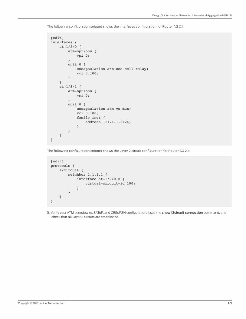
Copyright © 2013, Juniper Networks, Inc. 171
Design Guide - Juniper Networks Universal and Aggregation MBH 1.0
The following configuration snippet shows the interfaces configuration for Router AG 2.1:
[edit]interfaces { at-1/2/0 { atm-options { vpi 0; } unit 0 { encapsulation atm-ccc-cell-relay; vci 0.100; } } at-1/2/1 { atm-options { vpi 0; } unit 0 { encapsulation atm-vc-mux; vci 0.100; family inet { address 111.1.1.2/24; } } }}
The following configuration snippet shows the Layer 2 circuit configuration for Router AG 2.1:
[edit]protocols { l2circuit { neighbor 1.1.1.1 { interface at-1/2/0.0 { virtual-circuit-id 100; } } }}
3. Verify your ATM pseudowire, SAToP, and CESoPSN configuration; issue the show l2circuit connection command, and check that all Layer 2 circuits are established.

172 Copyright © 2013, Juniper Networks, Inc.
Design Guide - Juniper Networks Universal and Aggregation MBH 1.0
Configuring Timing and Synchronization The timing and synchronization configuration described in this chapter is independent of any particular deployment
scenario for a service level—4G LTE, HSPA, 3G, 2G—or any protocols at the transport level—OSPF, IS-IS, RSVP, BGP-LU,
or LDP DOD—which means that you can use this configuration in any of these deployment scenarios.
To propagate timing and synchronization from the grandmaster to eNodeB, NodeB, or BTS across the mobile backhaul
(MBH) network, you can choose between the following protocols:
• IEEE 1588v2 Precision Timing Protocol (PTP)
• Synchronous Ethernet
Configuring PTP Timing
The configuration in this deployment scenario is based on the network topology in Figure 73. You can use this
configuration in scenarios with 4G LTE or HSPA mobile networks.
eNodeB
NodeB
CSR 1.3
CSR 1.5
1588v2Grandmaster
AG 1.2
CSR 1.2 CSR 1.1 AG 1.1
CSR 1.4
10.1.1.1/2410.21.2.2/2410.21.1.1/24ge-0/1/0ge-0/2/0
10.21.4.0/24ge-0/2/0
10.21.2.1/24ge-0/2/0
10.21.0.2/24ge-0/2/1
10.21.6.2/24ge-0/2/1
10.21.0.1/24ge-0/2/1
10.21.5.2/24ge-0/2/1
10.21.5.1/24ge-0/2/0
10.21.1.2/24ge-0/2/0
10.21.6.1/24ge-0/2/0
ge-1/0/2
10.22.4.1/24ge-0/2/0
ge-1/0/3
10.22.1.1/24xe-0/0/0.2
10.22.0.2/24xe-0/0/0.2
ge-0/1/0
ge-0/1/0
Primary 1588v2 Source
Secondary 1588v2 Source
10.21.3.1/24xe-0/0/0.1
10.21.3.2/24xe-0/0/0.1
Figure 73: PTP design overview
The network example in Figure 73 includes only PTP over IPv4. The AG routers are the PTP source and the CSRs are the
PTP clients. Each CSR has interfaces configured to receive synchronization from either AG 1.1 or AG 1.2. Because a CSR
uses only one source at any given time, the CSR selects the best or nearest source for the PTP packets. The solid and
dashed lines represent the PTP sessions established between the AG routers and the CSRs. The solid lines represent
the active PTP sessions. The dashed lines represent the backup PTP sessions. This network configuration has the
following characteristics:
1. The grandmaster (GM) is connected to Router AG 1.1.
2. Router AG 1.1 acts in boundary clock mode.
3. Router AG 1.2 is an IEEE 1588v2 slave to Router AG 1.1 and acts in boundary clock mode.
4. Each CSR acts in boundary clock mode with the following characteristics:
a. A Gigabit Ethernet interface facing Router AG 1.1 configured as an IEEE 1588v2 slave, with Router AG 1.1 router as the IEEE 1588v2 master.
b. A Gigabit Ethernet interface facing Router AG 1.2 configured as an IEEE 1588v2 slave, with Router AG 1.2 as the IEEE 1588v2 master.
c. Interface ge-0/1/0.0 configured as the PTP master, providing synchronization to eNodeB or NodeB.

Copyright © 2013, Juniper Networks, Inc. 173
Design Guide - Juniper Networks Universal and Aggregation MBH 1.0
To configure PTP timing:
1. Configure Router AG 1.1 and Router AG 1.2 as boundary clocks, with the IPv4 PTP grandmaster located behind Router AG 1.1:
a. Configure Router AG 1.1 with interfaces acting as PTP slaves.
b. Configure Router AG 1.1 as a PTP master for all IEEE 1588v2 peers—all CSRs and Router AG 1.2.
The following configuration snippet shows the PTP configuration for Router AG 1.1:
[edit]protocols { ptp { clock-mode boundary; domain 0 slave { delay-request -6; interface ge-1/0/3.0 { unicast-mode { transport ipv4; clock-source 10.1.1.2 local-ip-address 10.1.1.1; } } } master { interface ge-1/0/2.0 { unicast-mode { transport ipv4; clock-client 10.21.2.1/32 local-ip-address 10.21.2.2; clock-client 10.21.1.1/32 local-ip-address 10.21.2.2; clock-client 10.21.0.1/32 local-ip-address 10.21.2.2; clock-client 10.21.6.1/32 local-ip-address 10.21.2.2; clock-client 10.21.5.1/32 local-ip-address 10.21.2.2; } } interface xe-0/0/0.1 { unicast-mode { transport ipv4; clock-client 10.21.3.2/32 local-ip-address 10.21.3.1; } }
} }}
The following configuration snippet shows the PTP configuration for Router AG 1.2:
[edit]protocols { ptp { clock-mode boundary; slave { delay-request -6; interface xe-0/0/0.1 { unicast-mode { transport ipv4; clock-source 10.21.3.1 local-ip-address 10.21.3.2; } }

174 Copyright © 2013, Juniper Networks, Inc.
Design Guide - Juniper Networks Universal and Aggregation MBH 1.0
} master { interface ge-1/0/2.0 { unicast-mode { transport ipv4; clock-client 10.21.4.2/32 local-ip-address 10.21.4.1; clock-client 10.21.5.2/32 local-ip-address 10.21.4.1; clock-client 10.21.6.2/32 local-ip-address 10.21.4.1; clock-client 10.21.0.2/32 local-ip-address 10.21.4.1; clock-client 10.21.1.2/32 local-ip-address 10.21.4.1; } } } }}
2. Configure each CSR with boundary clock mode as follows:
a. Configure each CSR boundary clock to act as a slave dual homed to both Router AG 1.1 and Router AG 1.2 master clocks.
b. Configure a CSR to act as a master clock for eNodeB.
The following configuration snippet shows the PTP configuration for Router CSR 1.2. You can use the configuration as
the basis for the PTP configuration of all other CSRs—CSR 1.1, CSR 1.3, CSR 1.4, and CSR 1.5. However, you must change
the router-specific details to match a particular CSR.
[edit]protocols { ptp { clock-mode boundary; domain 0; unicast-negotiation; slave { delay-request -6; sync-interval -6; grant-duration 300; interface ge-0/2/0.0 { unicast-mode { transport ipv4; clock-source 10.21.2.2 local-ip-address 10.21.1.1; } } interface ge-0/2/1.0 { unicast-mode { transport ipv4; clock-source 10.21.4.1 local-ip-address 10.21.0.2; } } } master { interface ge-0/1/0.0 { unicast-mode { transport ipv4; clock-client 10.0.3.1/32 local-ip-address 10.0.3.2; } } } }}

Copyright © 2013, Juniper Networks, Inc. 175
Design Guide - Juniper Networks Universal and Aggregation MBH 1.0
4. To verify your timing and synchronization setup, issue the show ptp clock and show ptp lock-status commands, and check the following sessions and status:
a. Verify that the PTP sessions are up.
b. Verify that the PTP lock status goes into the phase-aligned state.
c. Measure the amount of time it takes to get to the phase-aligned state.
d. Verify that CSRs can be both IEEE 1588v2 master and IEEE 1588v2 slave.
e. Make sure that all the clocking is stabilized and all the devices are in the phase-aligned state.
Configuring Synchronous Ethernet
Synchronous Ethernet is agnostic to upper layer protocols and has the same configuration for all deployment
scenarios—4G LTE, HSPA, 3G, or 2G—which means that you can use this configuration in any of these deployment
scenarios. Figure 74 illustrates a deployment scenario for Synchronous Ethernet.
CSR 1.3
AG 1.4
CSR 1.2 CSR 1.1 AG 1.3
CSR 1.4 CSR 1.5
AG 1.1 AG 2.1
AG 2.2AG 1.2
eNodeB
NodeB
ge-0/1/0
ge-0/1/0ge-0/2/0
ge-2/0/0
ge-2/0/0
ge-0/2/1
10.21.1.1/24
10.21.1.2/24
ge-0/2/0
ge-1/0/2
10.21.2.1/24
10.21.2.2/24
xe-0/0/2
xe-0/0/2
10.22.1.1/24
10.22.1.2/24
xe-0/0/0.110.21.3.1/24
xe-0/0/0.121.0.3.2/24
xe-0/0/0.210.22.0.1/24
xe-0/0/0.210.22.0.2/24
ge-0/2/1
ge-1/0/2
10.21.4.2/24
10.21.4.1/24ge-0/2/0
10.21.5.1/24
ge-0/2/010.21.0.1/24
ge-0/2/121.0.0.2/24
ge-0/2/021.0.6.1/24
ge-0/2/110.21.5.2/24
ge-0/2/110.21.6.2/24
ge-0/1/0xe-0/0/2
xe-0/0/2
10.22.5.2/24
10.22.5.1/24
xe-0/0/0
xe-0/0/0
10.22.2.1/24
10.22.2.2/24
xe-0/0/0
xe-0/0/0
10.22.4.2/24
10.22.4.1/24
xe-0/0/010.22.3.1/24
xe-0/0/010.22.3.2/24
SyncE
Io0: 1.1.1.1/32Grandmaster
Figure 74: Synchronous Ethernet deployment topology
In Figure 74, you connect the grandmaster (GM) with Gigabit Ethernet optical interfaces to the aggregation routers
AG 2.1 and AG 2.2. After you have configured and enabled Synchronous Ethernet on ACX Series or MX Series routers,
all 10GbE and 1GbE interfaces on the router transmit the Synchronous Ethernet signal to directly connected neighbors.
Figure 74 shows the distribution of synchronization in the sample topology.
The following configuration snippet shows the Synchronous Ethernet configuration for Router AG 2.1. You can use the
same basic configuration for all the other AG 1, AG 2, and AG 3 routers. However, you must change the router-specific
details (such as synchronization source interface) to match a particular router.
[edit]chassis { synchronization { network-option option-1; quality-mode-enable; source { interfaces ge-2/0/0 { wait-to-restore 1; quality-level prc; } interfaces xe-0/0/1 {
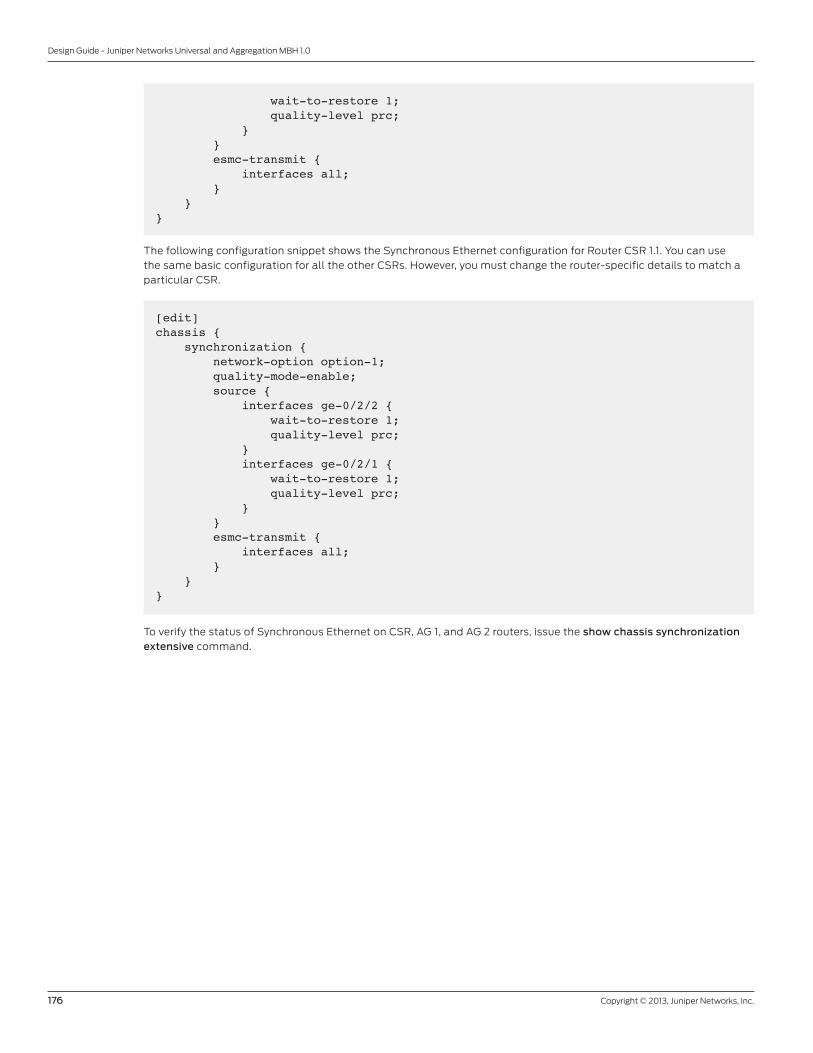
176 Copyright © 2013, Juniper Networks, Inc.
Design Guide - Juniper Networks Universal and Aggregation MBH 1.0
wait-to-restore 1; quality-level prc; } } esmc-transmit { interfaces all; } }}
The following configuration snippet shows the Synchronous Ethernet configuration for Router CSR 1.1. You can use
the same basic configuration for all the other CSRs. However, you must change the router-specific details to match a
particular CSR.
[edit]chassis { synchronization { network-option option-1; quality-mode-enable; source { interfaces ge-0/2/2 { wait-to-restore 1; quality-level prc; } interfaces ge-0/2/1 { wait-to-restore 1; quality-level prc; } } esmc-transmit { interfaces all; } }}
To verify the status of Synchronous Ethernet on CSR, AG 1, and AG 2 routers, issue the show chassis synchronization extensive command.

Copyright © 2013, Juniper Networks, Inc. 177
Design Guide - Juniper Networks Universal and Aggregation MBH 1.0
Configuring Class of Service In this example, the traffic from each mobile network service—such as S1-MME, S1-U, X2 Layer 2 or Layer 3 VPNs;
CESoPSN, SAToP ATM pseudowires; or MPLS Layer 3 VPN dedicated to network management system traffic—has
its own code points defined. The code points are defined according to 802.1p (RFC 2474), IP Differentiated Services
(DSCP), or experimental (EXP) bits located in each MPLS packet header. All the deployment scenarios described in
this guide support 802.1p or MPLS EXP bits.
In addition, you can add DSCP to enforce class-of-service (CoS) distinctions in routers. DSCP is fully supported on ACX
Series and MX Series routers. In the sample topology, a minimum configuration for CoS is included. However, an actual
network might need a more sophisticated CoS design, which is beyond the scope of this guide. As far as user traffic
having its own code points at the user-to-network interface (UNI) is concerned, the goals of this CoS design are:
1. Preserve these code points across the backhaul network.
2. Act upon these code points when faced with congestion.
3. Provide priority, low latency, and so on, in the network for a certain code point to reduce the jitter.
Configuring Class of Service on Cell Site Routers
Any node in the network can serve as a transit node serving CoS at the network-to-network interface (NNI), the UNI,
or as an access node. So from the class of service perspective, all nodes have identical configurations across the MBH
network. For detailed information about CoS, see the Junos OS Class of Service Configuration Guide.
The routers across the sample topology (Figure 75) have the following CoS configuration characteristics:
1. Five forwarding classes across the network—X2, S1, OAM, network-control, and default
2. Traffic classification and forwarding class assignment on the ingress UNI based on 802.1p
3. MPLS packets marking with EXP bit on egress NNI defined by rewrite rules of the CoS configuration of the router
4. Transit MPLS traffic classification and forwarding class assignment on the ingress NNI based on MPLS EXP
5. Traffic marking with 802.1p (or DSCP) code on the egress UNI defined by rewrite rules of the CoS configuration of the router

178 Copyright © 2013, Juniper Networks, Inc.
Design Guide - Juniper Networks Universal and Aggregation MBH 1.0
ACCESS COREPRE-AGGREGATION AGGREGATION
ds-0/0/3:1
CSR 1.3
EPC
Io0: 1.1.1.1/32
AG 1.1 AG 2.1 AG 3.1CSR 1.1CSR 1.2 AG 1.3
CSR 1.5CSR 1.4 AG 3.2AG 1.2 AG 1.4 AG 2.2
RNC/BSC
Io0:1.1.4.1/32 Io0:1.1.10.1/32Io0:1.1.2.1/32 Io0:1.1.3.1/32 Io0:1.1.8.1/32 Io0:1.1.13.1/32
Io0:1.1.5.1/32 Io0:1.1.11.1/32Io0:1.1.7.1/32 Io0:1.1.6.1/32 Io0:1.1.9.1/32 Io0:1.1.14.1/32
ds-0/0/0:1e1-0/0/1
e1-0/0/10ge-0/1/0
ge-0/1/0ge-0/2/0
ge-2/0/0
ge-2/0/0
ge-0/2/110.21.1.1/24
10.21.1.2/24
ge-0/2/0
ge-1/0/210.21.2.1/24
10.21.2.2/24
xe-0/0/2
xe-0/0/210.22.1.1/24
10.22.1.2/24
ds-1/2/5:1 at-1/2/0e1-1/2/10e1-1/2/6
ds-1/2/0:1e1-1/2/10e1-1/2/1
10.22.0.1/2410.21.3.1/24
10.22.0.2/2410.21.3.2/24
ge-0/2/1
ge-1/0/2
10.21.4.2/24
10.21.4.1/24ge-0/2/0
10.21.5.1/24
ge-0/2/010.21.0.1/24
ge-0/2/110.21.5.2/24
ge-0/2/110.21.6.2/24
e1-0/0/1e1-0/0/10ge-0/1/0
xe-0/0/2
xe-0/0/2
10.22.5.2/24
10.22.5.1/24
xe-0/0/0
xe-0/0/010.22.2.1/24
10.22.2.2/24
xe-0/0/0
xe-0/0/0
10.22.4.2/24
10.22.4.1/24
xe-0/0/2
xe-1/0/210.23.3.1/24
10.23.3.2/24
xe-1/0/010.23.4.1/24
xe-1/0/010.23.4.2/24
xe-0/0/2
xe-1/1/3
10.23.5.1/24
10.23.5.2/24
xe-0/0/3
xe-0/0/0.2
xe-0/0/0.2
xe-0/0/0.1
xe-0/0/0.1
10.23.1.1/24
xe-1/1/110.23.1.2/24
xe-0/0/310.23.2.1/24
xe-1/1/310.23.2.2/24
at-0/0/16
802.1p802.1p EXP EXP EXP EXP EXP
802.1p802.1p EXP EXP EXP EXP EXP
Tra�c Flow
802.1p Classifier ieee-802.1
cl_dot1p
Classify CircuitEmulatedTra�c toDEF class
802.1pRewrite:
ieee-802.1rw_dot1p
802.1pClassifier:ieee-802.1
c1_dot1p
EXPClassifier
exp c1_exp
EXP Rewrite:
exp rw_exp
Classify CircuitEmulatedTra�c toDEF class
xe-0/0/110.22.3.1/24
xe-0/0/110.22.3.2/24
Figure 75: Topology for CoS
To configure CoS on the routers in the CSR ring:
1. Configure forwarding classes and assign each of the classes to one of eight possible queues. (Both network control traffic and IEEE 1588v2 PTP go to queue three by default; OAM traffic goes to queue two by default).
2. Configure classifiers to map traffic code points to different forwarding classes at the ingress UNI and NNI.
The following configuration snippet shows the classifiers and forwarding class configuration for any CSR in the access
segment of the sample topology:
[edit]class-of-service { classifiers { exp cl_exp { forwarding-class S1 { loss-priority low code-points 011; } forwarding-class X2 { loss-priority low code-points 001; }
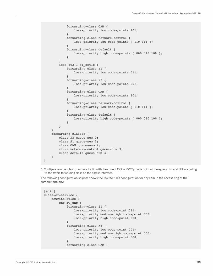
Copyright © 2013, Juniper Networks, Inc. 179
Design Guide - Juniper Networks Universal and Aggregation MBH 1.0
forwarding-class OAM { loss-priority low code-points 101; } forwarding-class network-control { loss-priority low code-points [ 110 111 ]; } forwarding-class default { loss-priority high code-points [ 000 010 100 ]; } } ieee-802.1 cl_dot1p { forwarding-class S1 { loss-priority low code-points 011; } forwarding-class X2 { loss-priority low code-points 001; } forwarding-class OAM { loss-priority low code-points 101; } forwarding-class network-control { loss-priority low code-points [ 110 111 ]; } forwarding-class default { loss-priority high code-points [ 000 010 100 ]; } } } forwarding-classes { class X2 queue-num 0; class S1 queue-num 1; class OAM queue-num 2; class network-control queue-num 3; class default queue-num 4; }}
3. Configure rewrite rules to re-mark traffic with the correct EXP or 802.1p code point at the egress UNI and NNI according to the traffic forwarding class on the egress interface.
The following configuration snippet shows the rewrite rules configuration for any CSR in the access ring of the
sample topology:
[edit]class-of-service { rewrite-rules { exp rw_exp { forwarding-class S1 { loss-priority low code-point 011; loss-priority medium-high code-point 000; loss-priority high code-point 000; } forwarding-class X2 { loss-priority low code-point 001; loss-priority medium-high code-point 000; loss-priority high code-point 000; } forwarding-class OAM {

180 Copyright © 2013, Juniper Networks, Inc.
Design Guide - Juniper Networks Universal and Aggregation MBH 1.0
loss-priority low code-point 101; loss-priority medium-high code-point 101; loss-priority high code-point 101; } forwarding-class network-control { loss-priority low code-point 111; loss-priority medium-high code-point 110; loss-priority high code-point 110; } forwarding-class default { loss-priority low code-point 000; loss-priority high code-point 000; loss-priority medium-high code-point 000; } } ieee-802.1 rw_dot1p { forwarding-class S1 { loss-priority low code-point 011; loss-priority medium-high code-point 000; loss-priority high code-point 000; } forwarding-class X2 { loss-priority low code-point 001; loss-priority medium-high code-point 000; loss-priority high code-point 000; } forwarding-class OAM { loss-priority low code-point 101; loss-priority medium-high code-point 101; loss-priority high code-point 101; } forwarding-class network-control { loss-priority low code-point 111; loss-priority medium-high code-point 110; loss-priority high code-point 110; } forwarding-class default { loss-priority low code-point 000; loss-priority high code-point 000; loss-priority medium-high code-point 000; } } }}
4. Configure schedulers and scheduler maps to define rules about how to manage traffic queues for each forwarding class.
The following configuration snippet shows the schedulers configuration for any CSR in the access segment of the
sample topology:
[edit]class-of-service { scheduler-maps { mbh { forwarding-class X2 scheduler X2; forwarding-class S1 scheduler S1; forwarding-class OAM scheduler OAM;

Copyright © 2013, Juniper Networks, Inc. 181
Design Guide - Juniper Networks Universal and Aggregation MBH 1.0
forwarding-class network-control scheduler NC; forwarding-class default scheduler DEF; } } schedulers { X2 { transmit-rate percent 35; buffer-size percent 35; } S1 { transmit-rate percent 35; buffer-size percent 35; } OAM { transmit-rate percent 5; shaping-rate percent 5; buffer-size temporal 10k; priority strict-high; } NC { transmit-rate percent 10; buffer-size percent 10; priority strict-high; } DEF { transmit-rate { remainder; } buffer-size { remainder; } } }}
5. Configure a traffic shaper (optional—might be required if you use microwave lines in the access segment).
6. Configure traffic control profiles (optional—might be required if you define shapers).
7. Assign classifiers and rewrite rules to the UNIs and the NNIs.
8. Attach schedulers or traffic control profiles to the UNIs.
9. Attach schedulers or traffic control profiles to the NNIs.
The following configuration snippet shows the classifier, rewrite rule, and scheduler configuration on the interfaces on Router CSR 1.2. You can use the same basic configuration for all the other CSRs. However, you must change the
router-specific details (such as family inet address) to match a particular CSR:
[edit]class-of-service { system-defaults { classifiers { exp cl_exp; } } interfaces { ge-0/1/0 { classifiers { ieee-802.1 cl_dot1p; }

182 Copyright © 2013, Juniper Networks, Inc.
Design Guide - Juniper Networks Universal and Aggregation MBH 1.0
rewrite-rules { ieee-802.1 rw_dot1p; } } ge-0/2/0 { scheduler-map mbh; unit 0 { rewrite-rules { exp rw_exp; } } } ge-0/2/1 { scheduler-map mbh; unit 0 { rewrite-rules { exp rw_exp; } } } }}
10. Configure classification for TDM and ATM Layer 2 circuits. In the configuration example, traffic for TDM and ATM pseudowires goes to a default forwarding class. In an actual network, you might need to configure a separate forwarding class with a high-priority queue.
The following configuration snippet shows the configuration of CoS on IMA group interfaces for Router CSR 1.3:
[edit]class-of-service { interfaces { ds-0/0/0:1 { unit 0 { forwarding-class DEF; } } e1-0/0/1 { unit 0 { forwarding-class DEF; } } e1-0/0/10 { unit 0 { forwarding-class DEF; } } at-0/0/16 { unit 0 { forwarding-class DEF; } } }}
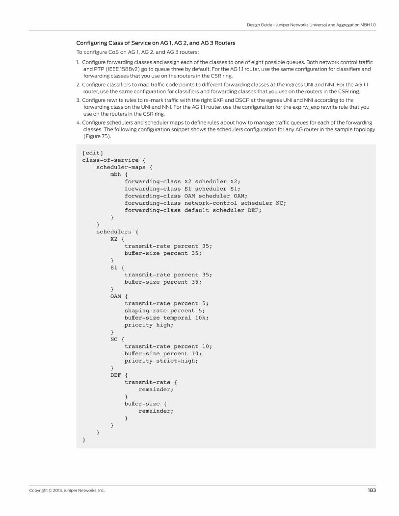
Copyright © 2013, Juniper Networks, Inc. 183
Design Guide - Juniper Networks Universal and Aggregation MBH 1.0
Configuring Class of Service on AG 1, AG 2, and AG 3 Routers
To configure CoS on AG 1, AG 2, and AG 3 routers:
1. Configure forwarding classes and assign each of the classes to one of eight possible queues. Both network control traffic and PTP (IEEE 1588v2) go to queue three by default. For the AG 1.1 router, use the same configuration for classifiers and forwarding classes that you use on the routers in the CSR ring.
2. Configure classifiers to map traffic code points to different forwarding classes at the ingress UNI and NNI. For the AG 1.1 router, use the same configuration for classifiers and forwarding classes that you use on the routers in the CSR ring.
3. Configure rewrite rules to re-mark traffic with the right EXP and DSCP at the egress UNI and NNI according to the forwarding class on the UNI and NNI. For the AG 1.1 router, use the configuration for the exp rw_exp rewrite rule that you use on the routers in the CSR ring.
4. Configure schedulers and scheduler maps to define rules about how to manage traffic queues for each of the forwarding classes. The following configuration snippet shows the schedulers configuration for any AG router in the sample topology (Figure 75).
[edit]class-of-service { scheduler-maps { mbh { forwarding-class X2 scheduler X2; forwarding-class S1 scheduler S1; forwarding-class OAM scheduler OAM; forwarding-class network-control scheduler NC; forwarding-class default scheduler DEF; } } schedulers { X2 { transmit-rate percent 35; buffer-size percent 35; } S1 { transmit-rate percent 35; buffer-size percent 35; } OAM { transmit-rate percent 5; shaping-rate percent 5; buffer-size temporal 10k; priority high; } NC { transmit-rate percent 10; buffer-size percent 10; priority strict-high; } DEF { transmit-rate { remainder; } buffer-size { remainder; } } }}
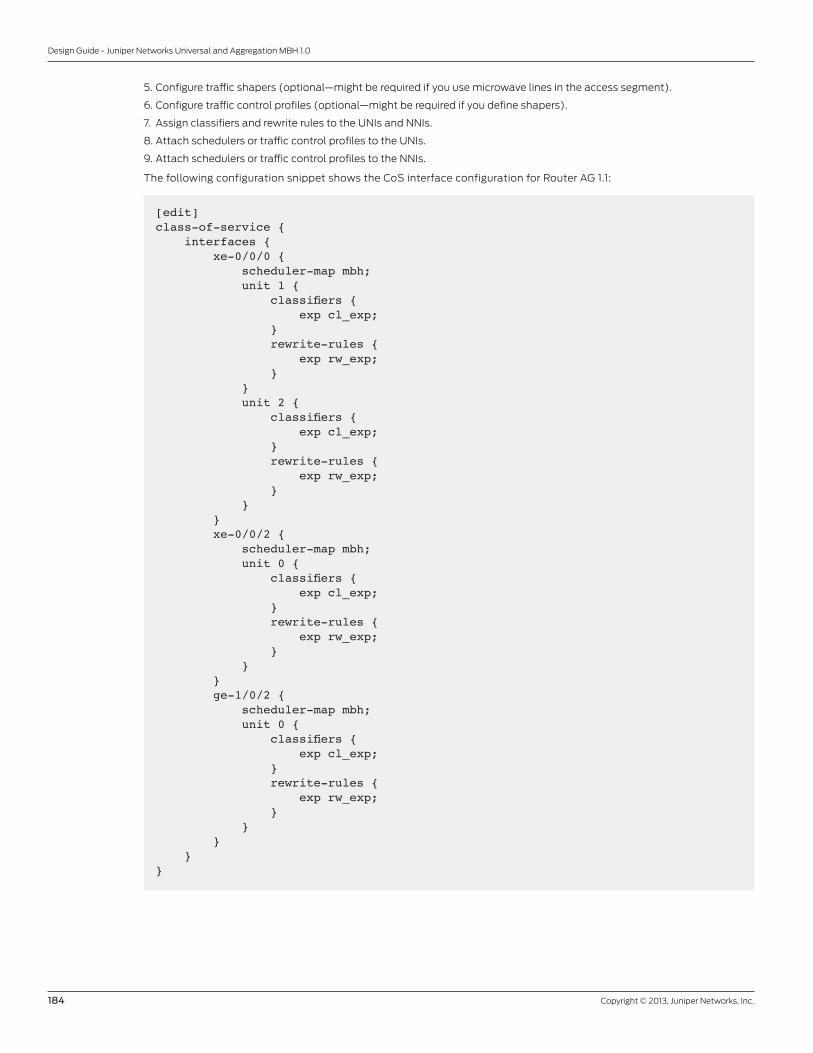
184 Copyright © 2013, Juniper Networks, Inc.
Design Guide - Juniper Networks Universal and Aggregation MBH 1.0
5. Configure traffic shapers (optional—might be required if you use microwave lines in the access segment).
6. Configure traffic control profiles (optional—might be required if you define shapers).
7. Assign classifiers and rewrite rules to the UNIs and NNIs.
8. Attach schedulers or traffic control profiles to the UNIs.
9. Attach schedulers or traffic control profiles to the NNIs.
The following configuration snippet shows the CoS interface configuration for Router AG 1.1:
[edit]class-of-service { interfaces { xe-0/0/0 { scheduler-map mbh; unit 1 { classifiers { exp cl_exp; } rewrite-rules { exp rw_exp; } } unit 2 { classifiers { exp cl_exp; } rewrite-rules { exp rw_exp; } } } xe-0/0/2 { scheduler-map mbh; unit 0 { classifiers { exp cl_exp; } rewrite-rules { exp rw_exp; } } } ge-1/0/2 { scheduler-map mbh; unit 0 { classifiers { exp cl_exp; } rewrite-rules { exp rw_exp; } } } }}

Copyright © 2013, Juniper Networks, Inc. 185
Design Guide - Juniper Networks Universal and Aggregation MBH 1.0
10. Configure classification for TDM and ATM Layer 2 circuits. In the configuration example, traffic for TDM and ATM pseudowires goes to a default forwarding class. In an actual network, you might need to configure a separate forwarding class with a high-priority queue.
The following configuration snippet shows the TDM interfaces configuration for Router AG 1.1:
[edit]class-of-service { interfaces { ds-1/2/5:1 { unit 0 { forwarding-class DEF; } } e1-1/2/6 { unit 0 { forwarding-class DEF; } } e1-1/2/10 { unit 0 { forwarding-class DEF; } }}
The following configuration snippet shows the ATM interfaces configuration for Router AG 2.1:
[edit]class-of-service { interfaces { at-1/2/0 { unit 0 { forwarding-class DEF; } } }}
11. Verify the configuration of CoS; issue the show interface interface-name extensive command. Specify the core or
customer-facing interfaces for the interface-name option.

186 Copyright © 2013, Juniper Networks, Inc.
Design Guide - Juniper Networks Universal and Aggregation MBH 1.0
8020018-002-EN Nov 2013
Copyright 2013 Juniper Networks, Inc. All rights reserved. Juniper Networks, the Juniper Networks logo, Junos and QFabric are registered trademarks of Juniper Networks, Inc. in the United States and other countries. All other trademarks, service marks, registered marks, or registered service marks are the property of their respective owners. Juniper Networks assumes no responsibility for any inaccuracies in this document. Juniper Networks reserves the right to change, modify, transfer, or otherwise revise this publication without notice.
APAC and EMEA Headquarters
Juniper Networks International B.V.
Boeing Avenue 240
1119 PZ Schiphol-Rijk
Amsterdam, The Netherlands
Phone: 31.0.207.125.700
Fax: 31.0.207.125.701
Corporate and Sales Headquarters
Juniper Networks, Inc.
1194 North Mathilda Avenue
Sunnyvale, CA 94089 USA
Phone: 888.JUNIPER (888.586.4737)
or 408.745.2000
Fax: 408.745.2100
www.juniper.net
Printed on recycled paper
To purchase Juniper Networks solutions,
please contact your Juniper Networks
representative at 1-866-298-6428 or
authorized reseller.


![Index [assets.cambridge.org]assets.cambridge.org/97805218/60253/index/9780521860253_index… · aggregation. See bubble, aggregation; particle, aggregation; particle, concentration](https://img.dokumen.tips/doc/110x75/60634dbbe29a93467d378f87/index-aggregation-see-bubble-aggregation-particle-aggregation-particle.jpg)