United States Patent US 6,892,163 B1 - NASA12) United States Patent Herzog et al. (io) Patent No.: (45) Date of Patent: US 6,892,163 B1 May 10,2005 (54 ... Wegerich, S., et al, Challenges

(12) United States Patent Herzog et al.

(io) Patent No.: (45) Date of Patent:

US 6,892,163 B1 May 10,2005

(54) SURVEILLANCE SYSTEM AND METHOD HAVING AN ADAPTIVE SEQUENTIAL PROBABILITY FAULT DETECTION TEST

Inventors: James P. Herzog, Downers Grove, IL (US); Randall L. Bickford, Orangevale, CA (US)

(73) Assignee: Intellectual Assets LLC, Lake Tahoe,

(75)

NV (US)

Subject to any disclaimer, the term of this patent is extended or adjusted under 35 U.S.C. 154(b) by 129 days.

( * ) Notice:

(21) Appl. No.: 10/095,835

(22) Filed: Mar. 8, 2002

(Under 37 CFR 1.47)

(51) Int. C1.7 ................................................ GOlR 17/00 (52) U.S. C1. .......................................... 702/181; 700130 (58) Field of Search .......................... 7021183, 72, 189,

7021185, 181; 700130, 29; 714126; 706115

(56) References Cited

U.S. PATENT DOCUMENTS

5,223,207 A * 611993 Gross et al. ................ 3761216 5,410,492 A * 411995 Gross et al. ................ 7021185 5,459,675 A * 1011995 Gross et al. 5,586,066 A * 1211996 White et al. 5,629,872 A * 511997 Gross et a1 5,680,409 A * 1011997 Qin et al. 5,745,382 A * 411998 Vilim et a1 5,761,090 A * 611998 Gross et al. 5,764,509 A * 611998 Gross et al. 5,774,379 A * 611998 Gross et al. 5,987,399 A * 1111999 Wegerich et al. ........... 7021183 6,107,919 A * 812000 Wilks et al. ................ 3401511 6,119,111 A * 912000 Gross et al. .................. 706115 6,131,076 A * 1012000 Stephan et al. ............. 7021189 6,181,975 B1 * 112001 Gross et al. .................. 700129 6,202,038 B1 * 312001 Wegerich et al. ........... 7021183 6,240,372 B1 * 512001 Gross et al. 702171 6,245,517 B1 * 612001 Chen et al. .................... 43516

6,609,036 B1 * 812003 Bickford ...................... 700130 6,625,569 B2 * 912003 James et al. ................ 7021183

200110049590 A1 * 1212001 Wegerich .................... 7021189 200410002776 A1 * 112004 Bickford ...................... 700130 200410006398 A1 * 112004 Bickford ...................... 700130

OTHER PUBLICATIONS

Hylko, J.M., New AI Technique Detects Instruments, Power, Nov. 1998, Printed in USA by Power. Herzog, J.P., et al, MSET Modeling of Crystal River-3 Venturi Flow Meters, 6th International Conference on Nuclear Engineering, 1998, Printed in USA by ASME. Bickford, R.L., et al, Real-Time Space Shuttle Main Engine Sensor Validation, National Aeronautics and Space Admin- istration, Augg. 1995, Printed in USA by ExperTech & Intelligent Software Associates, Inc. Bickford, R.L., et al, Real-Time Flight Data Validation For Rocket Engines, AIAA, 1996, Printed in USA by ExperTech & NYMA, Inc. Bickford, R.L., et al, Real-Time Sensor Validation for Autonomous Flight Control, AIAA, Jul. 1997, Printed in USA by Expert Microsystems, Inc. & Intelligent Software Associates, Inc. & Beoing Defense and Space Group. Bickford, R.L., et al, Real-Time Sensor Validation For Propulsion Systems, American Institute of Aeronautics and Astronautics, 1998, Printed in USA by Expert Microsys- tems, Inc & Dynacs Engineering Co.

(Continued)

Primary Examiner-John Barlow Assistant Examiner-Victor J. Taylor (74) Attorney, Agent, or F i r m 4 e n n i s A. DeBoo

(57) ABSTRACT

System and method providing surveillance of an asset such as a process andlor apparatus by providing training and surveillance procedures that numerically fit a probability density function to an observed residual error signal distribution that is correlative to normal asset operation and then utilizes the fitted probability density function in a dynamic statistical hypothesis test for providing improved asset surveillance.

32 Claims, 20 Drawing Sheets

i20 Aonel

https://ntrs.nasa.gov/search.jsp?R=20080005099 2018-06-18T13:00:16+00:00Z

US 6,892,163 B1 Page 2

OTHER PUBLICATIONS

Bickford, R.L., et al, Real-Time Sensor Data Validation For Space Shuttle Main Engine Telemetry Monitoring, AIAA, Jun. 1999, Printed in USA by Expert Microsystems, Inc.& Intelligent Software Associates, Inc. & Dynacs Engineering Company & NASA Glenn Research Center. Singer, R.M., et al, A Pattern-recognition-based, Fault-tol- erant Monitoring and Diagnostic Technique, 7th Symp. on Nuclear Reactor Surveillance, Jun. 1995, Printed in USA by Argonne National Laboratory. Bickford, R.L., et al, Online Signal Validation for Assured Data Integrity, 47th International Instrumentation Sympo- sium, May 2001, Printed in USA by Expert Microsystems, Inc., and NASA Glenn Research Center. Wegerich, S., et al, Challenges Facing Equipment Condition Monitoring Systems, MARCOM 2001, May 2001, Printed in USA by Smartsignal Corporation. Zavaljevski, N., et al, Sensor Fault Detection in Nuclear Power Plants Using Multivariate State Estimation Technique and Support Vector Machines, 3rd Intl. Conf. of Yugoslav Nuclear Society, Oct. 2000, Printed in USA by Argonne National Laboratory. Zavaljevski, N., et al, Support Vector Machines for Nuclear Reactor State Estimation, A N S Topical Mtg. on Advances in Reactor Physics, May 2000, Printed in USA by Argonne National Laboratory. Bickford, R.L., et al, Sensor Validation Tools and SSME Network, Final Report, Apr. 2000, Printed in USAby Expert Microsystems, Inc. Miron, A,, et al, The Effects of Parameter Variation on MSET Models of the Crystal River-3 Feedwater Flow System, A N S Annual Meeting, Jun. 1998, Printed in USAby Argonne National Laboratory. Wrest, D.J., et al., Instrument Surveillance and Calibration Verification through Plant Wide Monitoring Using Autoas- sociative Neural Networks, Specialists Meeting on Moni- toring and Diagnosis Systems to Improve Nuclear Power Plant Reliability and Safety, May 1996, printed by the International Atomic Energy Agency.

K. Humenik, et al, Sequential Probability Ratio Tests for Reactor Signal Validation and Sensor Surveillance Applica- tions, Nuclear Science and Engineering, vol. 105, pp

K.C. Gross, et al, Sequential Probability Ratio Test for Nuclear Plant Component Surveillance, Nuclear Technol- ogy, vol. 93, p. 131, Feb. 1991.

A. Racz, Comments on the Sequential Probability Ratio Testing Methods, Annals of Nuclear Energy, vol. 23, No. 11,

K. Kulacsy, Further Comments on the Sequential Probability Ratio Testing Methods, prepared for Annals of Nuclear Energy by the KFKI Atomic Energy Research Institute, Budapest, Hungary, Report No. KFKI-1O/G, 1996.

R. M. Singer, et al, Model-Based Nuclear Power Plant Monitoring and Fault Detection: Theoretical Foundations, Proceedings, 9th International Conference on Intelligent Systems Applications to Power Systems, Seoul, Korea, 1997.

K.C. Gross, et al, Application of a Model-based Fault Detection System to Nuclear Plant Signals, Proceedings 9th International Conference on Intelligent Systems Applica- tions to Power Systems, Seoul, Korea, 1997.

R. M. Singer, et al, Power Plant Surveillance and Fault Detection: Applications to a Commercial PWR, Interna- tional Atomic Energy Agency, IAEA-TECDOC-1054, pp. 185-200, Sep. 1997.

K. Kulacsy, Tests of the Bayesian Evaluation of SPRT Outcomes on PAKS NPP Data, KFKI Atomic Energy Research Institute, Budapest, Hungary, Report No.

J.P. Herzog, et al, Dynamics Sensor Validation for Reusable Launch Vehicle Propulsion, AIAA 98-3604, 34th Joint Propulsion Conference, Cleveland, Ohio, 1998.

* cited by examiner

383-390, 1990.

pp. 919-934, 1996.

KFKI-l99747/G, 1997.

U S . Patent May 10,2005

4

0

j

Sheet 1 of 20 US 6,892,163 B1

-7

1 t r

al L 3 0,

LL .d

U S . Patent May 10,2005 Sheet 2 of 20 US 6,892,163 B1

t L

T


I I I

1 % ! I \ I I I I I I I I I I I I

I I I

I

I 2 ’3

! U la 1 0 ‘ 2 la I

‘ 2 ) I .- I .E y

-)---

0 m

I I I / ” ! I I I I I I I I I I I I I I I I I

cv v)

t

J

/

c7

3 0 LL

2 .-


I I I I I I I I I I

I I I I I I L -

N m

L ---

I I I I I I I I I I I I I

I I I I

-1

S 0, LL .C


I’

1

0 h

U S . Patent May 10,2005 Sheet 6 of 20

(Y UY

3

c I - - - - - - - - -

I _ -

I

US 6,892,163 B1


F- a L 3


t

I m I

. I I

00 0 L


I Acquire and Store Asset Training Data - 1 1

Calibrate Parameter Estimator(s) (Procedure (36)) Using Asset Training Data And Training Procedure (e.g., MSET Training Procedure) For Producing Parameter Estimation Model(s)

Calibrate Fault Detector(s) (Procedure (38)) Including Fitting A General PDF To Computed Training Data Residual Distribution,

For Example By Fitting A Standard Gaussian PDF To The Computed Training Data Residuals And Then Adding Successive Higher Order Terms Of A Remainder Function To The Standard Gaussian PDF Until An Adequate Fit Between The General PDF And Computed Training Data Residual Distribution Is Produced

~ ~

It ~~

AcqGire and Digitize Current Asset Data I ~~

Estimate Process Parameters (Procedure (64)) Using Acquired and Digitized Current Asset Data And Parameter Estimation Model(s)

1 Perform Fault Detection (Procedure (66)) By Computing Data

Residuals (Procedure (76)) And Using The Fitted General PDF In Performing The Adaptive Sequential Probability (ASP) Test(s) (Procedure (78)) In Accordance With The Present Invention

Fault Found? Surveil lance Complete?

End Surveillance

Figure 9


0.i

O.!

0..

0.:

0.:

0.'

HO: Mean = 0, Variance = 1

H l : Mean = 2. Variance = 1 l - . . . . . . . . H2: Mean E -2, Variance = 1

-4 -2 0 2 4 6

Figure I O


0.1

O.!

0.C

0,:

0.2

0.3

HO: Mean = 0, Variance = 1 H3: Mean = 0, Variance = 2 H4; Mean = 0, Variance = .5

I _ _ - 3 - 1 - - . . - I I .. / '

-6 4 -2 0 2 4 6

Figure I 1


Sensor Signal I .

I I

-30

- 4 0

0 100 200 3aa 1oc 500 Time (sec)

MSET Estimate Signal I I I I I

I '

0 i o 0 200 300 400 so0 Titne (see)

Residual Signal I I

I I

0 100 200 300 400 500 Time (sec)

-0 .5

Figure 12


71 I 1 I I I I I

01 I I I

I -0.6 -0.4 -0.2 0 02 0.4 0.6 0.8 -0.8

Acceleration (g)

Figure 13


I

I ,

, I , . , , , , Residual Signal pdf Gaussian pdf 1 Term Expansion pdf

:\

Figure 14


x rA c .-

x .z 4 c1 3 4!

4 3 -

a E4 P

.M I

E 2 -

1 -

0 4 .8

Sheet 15 of 20

7 I I I I I I I

, I , , , , , , Residual Signal pdf

Gaussian pdf 2 Term Expansion pdf 6 -

! ! ! i r ! I 1 t I

5- I ! -

-

- -

I

-0.2 0 0.2 0.4 0.6 0.8 -0.6 -0.4

US 6,892,163 B1

9 !

c < I' r:

Figure 15


I I


Sensor Number

1

Sheet 17 of 20

One-Term Two-Term Three-Term Four-Term

Expansion Expansion Expansion Expansion Gaussian Series Series Series Series

0.414 0.409 0.122 0.151 2.06

US 6,892,163 B1

2

3

4

0.389 0.396 0.147 0.223 2.1 3

0.233 0.234 0.0605 0.065 1 0.171

0.339 0.320 0.0964 0.1 46 0.256

5

6

0.156 0.167 0.121 0.09S5 0.0983

0.180 0.134 0.107 0.326 0.656

Figure 17

U.S. Patent

Sensor Plumber

I

May 10,2005

One-Term Two-Term Three-Term Four-Term

Expansion Expansion Expansion Expansion Gaussian Series Series Series Series

0.414 0.176 0.0826 0.0755 0.0899

Sheet 18 of 20

~ ~~

1 3 1 0.233 1 0.122 I 0.0522 ~ 0 . 0 5 7 3 I --0.0522 I

US 6,892,163 B1

I 4 I 0.339 I 0.166 I 0.0706 1 0.0724 1 0.0713 I 3

4

5

6

1 2 1 0.389 I 0.174 1 0.081 1 I 0.0816 I 0.0659 I ~ ~~

0 233 0.122 0.0522 0.0573 0.0522

0.339 0.166 0.0706 0.0724 0.0713

0.156 0.0699 0.0394 0.0352 0.0373

0.180 0.0710 0.0346 0.0352 0.0369

5

6

0.156 0.0699 0.0394 0.0352 0.0373

0.180 0.0710 0.0346 0.0352 0.0369

Figure I 8


P ' I . , , * . , Residual Signal pdf

Gaussian pdf Optimized 2 Term pdf

I I I I

-0.6 -0.4 -0.2 0 0.2 0.4 0.6 0.8 Acceleration (6)

0 i -0.8

Figure I 9


loo 1

I 3

BSP Method SPRT Method Theoretical Upper Bound

lo-?

Figure 20

us 1

SURVEILLANCE SYSTEM AND METHOD HAVING AN ADAPTIVE SEQUENTIAL

PROBABILITY FAULT DETECTION TEST

STATEMENT REGARDING FEDERALLY SPONSORED RESEARCH AND

DEVELOPMENT

6,892,163 B1

The invention described herein was made in the performance of work under NASA Small Business Technology Transfer Research (STTR) Contract NAS8-98027, and is subject to the provisions of Public Law 96-517 (35 USC 202) and the Code of Federal Regulations 48 CFR 52.227-11 as modified by 48 CFR 1852.227-11, in which the contractor has elected to retain title.

The United States Government has rights in this invention pursuant to Contract No. W-31-109-ENG-38 between the United States Government and the University of Chicago representing Argonne National Laboratory.

FIELD OF THE INVENTION

The instant invention relates generally to a system and method for process fault detection using a statistically based decision test and, in particular, to a system and method for performing high sensitivity surveillance of an asset such as a process and/or apparatus wherein the surveillance is performed using an adaptive sequential probability (ASP) fault detection test comprised of a probability density function model empirically derived from a numerical analysis of asset operating data.

BACKGROUND OF THE INVENTION

Conventional process surveillance schemes are sensitive only to gross changes in the mean value of a process signal or to large steps or spikes that exceed some threshold limit value. These conventional methods suffer from either a large number of false alarms (if thresholds are set too close to normal operating levels) or from a large number of missed (or delayed) alarms (if the thresholds are set too expansively). Moreover, most conventional methods cannot perceive the onset of a process disturbance or sensor signal error that gives rise to a signal below the threshold level or an alarm condition. Most conventional methods also do not account for the relationship between measurements made by one sensor relative to another redundant sensor or between measurements made by one sensor relative to predicted values for the sensor.

Recently, improved methods for process surveillance have developed from the application of certain aspects of artificial intelligence technology. Specifically, parameter estimation methods have been developed using either statistical, mathematical or neural network techniques to learn a model of the normal patterns present in a system of process signals. After learning these patterns, the learned model is used as a parameter estimator to create one or more predicted (virtual) signals given a new observation of the actual process signals. Further, high sensitivity surveillance methods have been developed for detecting process and signal faults by analysis of a mathematical comparison between an actual process signal and its virtual signal counterpart. In particular, such a mathematical comparison is most often performed on a residual error signal computed as, for example, the difference between an actual process signal and its virtual signal counterpart.

Parameter estimation based surveillance schemes have been shown to provide improved surveillance relative to

2 conventional schemes for a wide variety of assets including industrial, utility, business, medical, transportation, financial, and biological systems. However, parameter estimation based surveillance schemes have in general shown

5 limited success when applied to complex processes. Appli- cants recognize and believe that this is because the parameter estimation model for a complex process will, in general, produce residual error signals having a non-Gaussian probability density function. Moreover, a review of the known prior-art discloses that virtually all such surveillance systems developed to date utilize or assume a Gaussian model of the residual error signal probability density function for fault detection. Hence, a significant shortcoming of the known prior-art is that, inter alia, parameter estimation based surveillance schemes will produce numerous false alarms due to the modeling error introduced by the assumption of a Gaussian residual error signal probability density function. The implication for parameter estimation based surveillance schemes is that the fault detection sensitivity must be significantly reduced to prevent false alarms thereby

20 limiting the utility of the method for process surveillance. An alternative for statistically derived fault detection models is to mathematically pre-process the residual error signals to remove non-Gaussian elements prior to using the residual error signals in the fault detection model; however this

25 approach requires an excess of additional processing and also limits the sensitivity of the surveillance method. Therefore, the implication of assuming a Gaussian residual error signal probability density function for a parameter estimation based surveillance scheme is simply that the system becomes less accurate thereby degrading the sensitivity and utility of the surveillance method.

Many attempts to apply statistical fault detection techniques to surveillance of assets such as industrial, utility, business, medical, transportation, financial, and biological processes have met with poor results in part because the fault detection models used or assumed a Gaussian residual error signal probability density function.

In one specific example, a multivariate state estimation technique based surveillance system for the Space Shuttle Main Engine’s telemetry data was found to produce numer-

40 ous false alarms when a Gaussian residual error fault detection model was used for surveillance. In this case, the surveillance system’s fault detection threshold parameters were desensitized to reduce the false alarm rate; however, the missed alarm rate then became too high for practical use

Moreover, current fault detection techniques for surveillance of assets such as industrial, utility, business, medical, transportation, financial, and biological processes either fail to recognize the surveillance performance limitations that

SO occur when a Gaussian residual error model is used or, recognizing such limitations, attempt to artificially conform the observed residual error data to fit the Gaussian model. This may be attributed, in part, to the relative immaturity of the field of artificial intelligence and computer-assisted

ss surveillance with regard to real-world process control applications. Additionally, a general failure to recognize the specific limitations that a Gaussian residual error model imposes on fault decision accuracy for computer-assisted surveillance is punctuated by an apparent lack of known

60 prior art teachings that address potential methods to over- come this limitation. In general, the known prior-art teaches computer-assisted surveillance solutions that either ignore the limitations of the Gaussian model for reasons of mathematical convenience or attempt to conform the actual

65 residual error data to artificial Gaussian model, for example, by using frequency domain filtering and signal whitening techniques.

10

30 . .

35

45 in the telemetry data monitoring application.

US 6,892,163 B1 3

For the foregoing reasons, there is a need for a surveillance system and method that overcomes the significant shortcomings of the known prior-art as delineated hereinabove.

SUMMARY OF THE INVENTION

The instant invention is distinguished over the known prior art in a multiplicity of ways. For one thing, the instant invention provides a surveillance system and method having a fault detection model of unconstrained probability density function form and having a procedure suitable for overcom- ing a performance limiting trade-off between probability density function modeling complexity and decision accuracy that has been unrecognized by the known prior-art. Specifically, the instant invention can employ any one of a plurality of residual error probability density function model forms, including but not limited to a Gaussian form, thereby allowing a surveillance system to utilize the model form best suited for optimizing surveillance system performance.

Moreover, the instant invention provides a surveillance system and method that uses a computer-assisted learning procedure to automatically derive the most suitable form of the residual error probability density function model by observation and analysis of a time sequence of process signal data and by a combination of a plurality of techniques. This ability enables surveillance to be performed by the instant invention with lower false alarm rates and lower missed alarm rates than can be achieved by the known prior-art systems and methods.

Thus, the instant invention provides a surveillance system and method that performs its intended function much more effectively by enabling higher decision accuracy. Further, the instant invention is suitable for use with a plurality of parameter estimation methods thereby providing a capabil- ity to improve the decision performance of a wide variety of surveillance systems.

In one preferred form, the instant invention provides a surveillance system and method that creates and uses, for the purpose of process surveillance, a multivariate state estimation technique parameter estimation method in combination with a statistical hypothesis test fault detection method having a probability density function model empirically derived from a numerical analysis of asset operating data.

Particularly, the instant invention provides a surveillance system and method for providing surveillance of an asset such as a process and/or apparatus by providing training and surveillance procedures.

In accordance with the instant invention, the training procedure is comprised of a calibrate parameter estimator procedure and a calibrate fault detector procedure.

The calibrate parameter estimator procedure creates a parameter estimation model(s) and trains a parameter estimation model by utilizing training data correlative to expected asset operation and, for example, utilizing a multivariate state estimation technique (MSET) procedure. The calibrate parameter estimator procedure further stores this model as a new parameter estimation model in a process model. The process model may contain one or more parameter estimation models depending upon design requirements. Additionally, each parameter estimation model contained in the process model may be created to implement any one of a plurality of parameter estimation techniques.

The calibrate fault detector procedure makes use of the parameter estimation models to provide estimated values for at least one signal parameter contained in the training data. Generally, the calibrate fault detector procedure will create

4 a separate and distinct fault detection model for each sensor or data signal associated with the asset being monitored for the presence of fault conditions during the surveillance procedure.

The calibrate fault detector procedure includes, for example, a method of fitting a standard Gaussian probability density function (PDF) to a training data residual distribution (computed as a function of estimated process parameters and the training data) and then adding successive

10 higher order terms of a remainder function to the standard Gaussian PDF for the purpose of defining a general PDF that better fits the computed training data residual distribution. Other techniques for fitting a general PDF to the training data are similarly feasible and useful in accordance with the

15 instant invention and include, for example, a technique for fitting a polynomial function to the training data.

The training procedure is completed when all training data has been used to calibrate the process model. At this point, the process model preferably includes parameter

2o estimation models and fault detection models for each sensor or data signal associated with the asset being monitored for the presence of fault conditions during the surveillance procedure. The process model is thereafter used for performing surveillance of the asset.

The surveillance procedure is performed using an adaptive sequential probability (ASP) fault detection test comprised of the general probability density function model empirically derived from a numerical analysis of the asset

The surveillance procedure acquires and digitizes current asset data and then estimates process parameters as a function of the acquired digitized current asset data and the parameter estimation model(s) obtained from the calibrate

35 parameter estimator procedure. Then, fault detection is determined by first computing data residuals as a function of the estimated process parameters and the acquired digitized current asset data and then performing the ASP test(s) as a function of the fault detection models and thus, as a function

4o of the fitted general PDF obtained in the calibrate fault detector procedure. Each ASP test returns one of three possible states: a not null state which rejects the probability that a null hypothesis is true and excepts an alternative hypothesis correlative to unexpected operation of the asset;

45 a null state which accepts the probability that a null hypothesis is true and excepts the null hypothesis correlative to expected operation of the asset; and an in-between state which excepts neither the null hypothesis nor the alternative hypothesis as being true and requires more data to reach a conclusion.

The results of the fault detection procedure are then analyzed according to the instant invention such that an alarm and/or a control action are taken when the analysis determines that the results indicate unexpected operation of

Hence, the instant invention is distinguished over the known prior-art by providing a surveillance system and method for performing surveillance of an asset by acquiring residual data correlative to expected asset operation; fitting

60 an equation to said acquired residual data; storing said fitted equation in a memory means; collecting a current set of observed signal data values from the asset; using said fitted equation in a sequential hypotheses test to determine if said current set of observed signal data values indicate unex-

65 pected operation of the asset indicative a fault condition; and outputting a signal correlative to each detected fault condition for providing asset surveillance.

5

23

3o training data.

55 the asset.

US 6,892,163 B1 5

OBJECTS OF THE INVENTION

Accordingly, the instant invention provides a new, novel and useful surveillance system and method having an adaptive sequential probability fault detection test.

In one embodiment of the instant invention the surveillance system and method includes an unconstrained form of a residual error probability density function model used in said surveillance system's fault detection method.

In one embodiment of the instant invention the surveillance system and method can perform high sensitivity surveillance of a wide variety of assets including industrial, utility, business, medical, transportation, financial, and biological processes and apparatuses wherein such process and/or apparatus asset preferably has at least one pair of redundant actual and/or virtual signals.

In one embodiment of the instant invention the surveillance system and method includes a statistical hypothesis test surveillance decision procedure that uses a fault detection model comprised of a probability density function model of a residual error signal that is of an unconstrained form.

In one embodiment of the instant invention the surveillance system and method creates an improved fault detection model for a process surveillance scheme using recorded operating data for an asset to train a fault detection model.

In one embodiment of the instant invention the surveillance system and method provides an improved system and method for surveillance of on-line, real-time signals, or off-line accumulated signal data.

In one embodiment of the instant invention the surveillance system and method provides an improved system and method for surveillance of signal sources and detecting a fault or error state of the signal sources enabling responsive action thereto.

In one embodiment of the instant invention the surveillance system and method provides an improved system and method for surveillance of signal sources and detecting a fault or error state of the asset processes and apparatuses enabling responsive action thereto.

In one embodiment of the instant invention the surveillance system and method provides an improved decision as to the accuracy or validity for at least one process signal parameter given an observation of at least one actual signal from the asset.

In one embodiment of the instant invention the surveillance system and method provides an improved system and method for ultra-sensitive detection of a fault or error state of signal sources and/or asset processes and apparatuses wherein the parameter estimation technique used for the generation of at least one virtual signal parameter is a multivariate state estimation technique (MSET) having any one of a plurality of pattern recognition matrix operators, training procedures, and operating procedures.

In one embodiment of the instant invention the surveillance system and method provides an improved system and method for ultra-sensitive detection of a fault or error state of signal sources and/or asset processes and apparatuses wherein the parameter estimation technique used for the generation of at least one virtual signal parameter is a neural network having any one of a plurality of structures, training procedures, and operating procedures.

In one embodiment of the instant invention the surveillance system and method provides an improved system and method for ultra-sensitive detection of a fault or error state of signal sources and/or asset processes and apparatuses

6 wherein the parameter estimation technique used for the generation of at least one virtual signal parameter is a mathematical process model having any one of a plurality of structures, training procedures, and operating procedures.

In one embodiment of the instant invention the surveillance system and method provides an improved system and method for ultra-sensitive detection of a fault or error state of signal sources and/or asset processes and apparatuses wherein the parameter estimation technique used for the

10 generation of at least one virtual signal parameter is an autoregressive moving average (ARMA) model having any one of a plurality of structures, training procedures, and operating procedures.

In one embodiment of the instant invention the surveil- 's lance system and method provides an improved system and

method for ultra-sensitive detection of a fault or error state of signal sources and/or asset processes and apparatuses wherein the parameter estimation technique used for the generation of at least one virtual signal parameter is a

2o Kalman filter model having any one of a plurality of structures, training procedures, and operating procedures.

In one embodiment of the instant invention the surveillance system and method provides a novel system and

25 method for using at least one of a plurality of methods to classify the state of a residual error signal produced by the mathematical difference between two signals, said two signals being either actual and/or predicted signals, into one of at least two categories.

In one embodiment of the instant invention the surveillance system and method provides a novel system and method to classify the state of a residual error signal wherein said classification is made to distinguish between a normal signal and a abnormal signal.

In one embodiment of the instant invention the surveillance system and method provides a novel system and method to classify the state of a residual error signal wherein said classification is performed using a statistical hypothesis test having any one of a plurality of probability density

40 function models, training procedures, and operating procedures.

In one embodiment of the instant invention the surveillance system and method provides a novel system and method to classify the state of a residual error signal wherein

45 said classification is performed using a probability density function model having any one of a plurality of structures, training procedures, and operating procedures.

5

30

35

BRIEF DESCRIPTION OF THE DRAWINGS

FIG. 1 is a block diagram of a surveillance system of a preferred embodiment in accordance with the instant invention.

FIG. 2 is a schematic functional flow diagram of a preferred embodiment in accordance with the instant invention.

FIG. 3 is a schematic functional flow diagram of a preferred method and system for training a process model consisting of at least one parameter estimation model and at

6o least one fault detection model using recorded observations of the actual process signals in accordance with the instant invention.

FIG. 4 is a schematic functional flow diagram of a method and system for the fault detection model training procedure

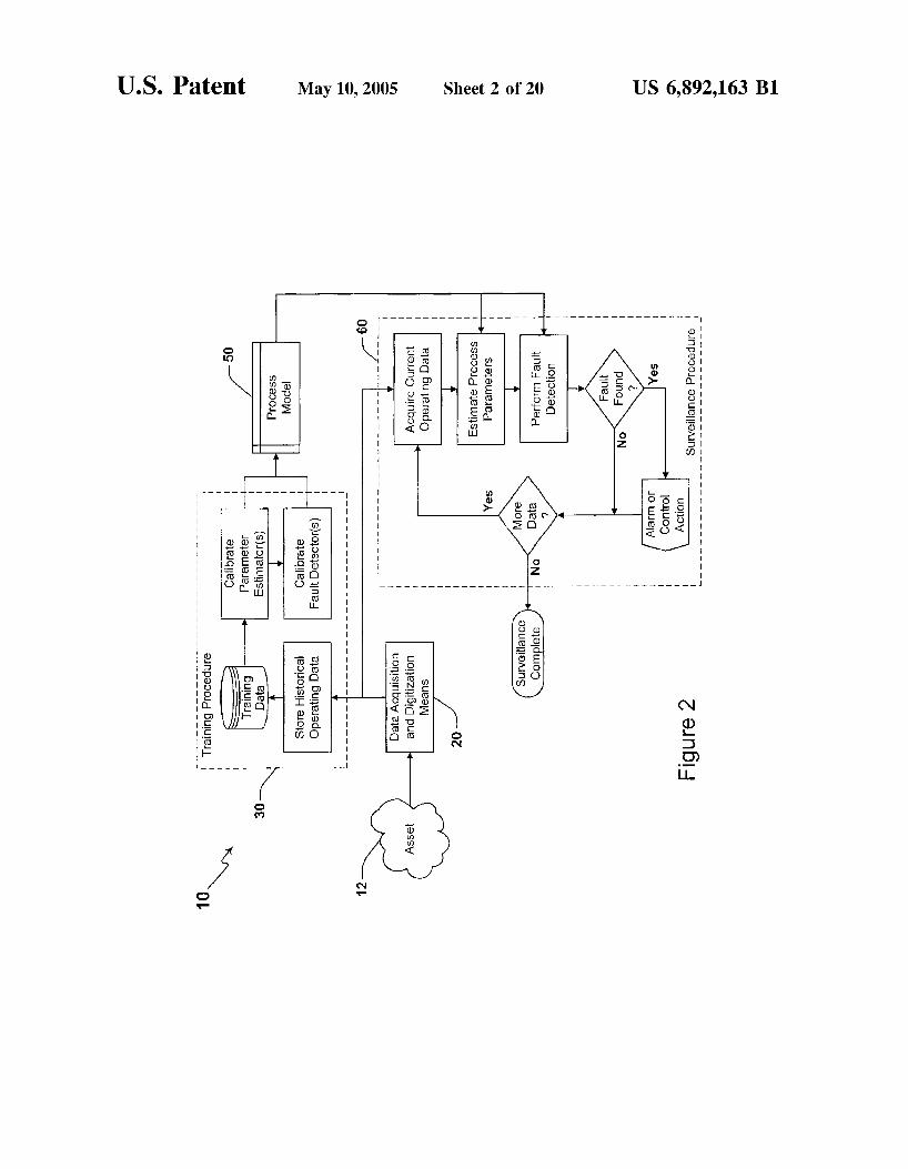
65 in accordance with the instant invention. FIG. 5 is a schematic functional flow diagram of a

preferred method and system for performing surveillance of

55 .

US 6,892,163 B1 7 8

an asset using at least one parameter estimation model and reference numeral 10 is directed to the system according to at least one fault detection model in accordance with the the instant invention. instant invention. In its essence, and referring to FIGS. 1 and 2, the system

FIG. 6 is a schematic functional flow diagram of a method 10 is generally comprised of a method and apparatus for and system for the fault detection surveillance procedure in 5 performing high sensitivity surveillance of a wide variety of accordance with the instant invention. assets including industrial, utility, business, medical,

FIG. 7 is a schematic functional flow diagram of a method transportation, financial, and biological processes and appa- and system for performing parameter estimation and fault ratuses wherein such process and/or apparatus asset prefer- detection using a redundant sensor. ably has at least one distinct measured or observed signal or

FIG. 8 is a schematic functional flow diagram of a method 10 sequence comprised of characteristic data values which are and system for performing parameter estimation and fault processed by the system 10 described herein for providing detection using a generalized Parameter estimation model, ultra-sensitive detection of the onset of sensor or data signal such as a multivariate State estimation model, a neural degradation, component performance degradation, and pro- network an Or a Kalman cess operating anomalies. The system 10 includes a training model. 1s procedure 30 carried out on a computer 22 such that a

FIG. 9 is a flow diagram of a training and surveillance process model 50 of an asset 12 (e.g., a process and/or procedure in accordance with the instant invention. apparatus) is stored in an associated memory means 24 after

FIG. 10 illustrates characteristics of the null and alternate being learned from historical operating data using at least hypotheses for the prior-art sequential probability ratio test one of a plurality of computer-assisted procedures in accor-

20 dance with the instant invention. The historical operating (SPRT) mean tests. FIG. 11 illustrates characteristics of the null and alternate data includes a set or range of observations from expected or

typical operation of the asset 12 that are acquired and hypotheses for the prior-art SPRT variance tests. FIG. 12 illustrates acquired operating data, estimated digitized by a data acquisition 20 and stored in a

2s nation of electronic data acquisition hardware and signal parameter data, and residual error data for a typical Space memory means 24 as training data 34 by using any combi- Shuttle Main Engine accelerometer.

l3 a probability density function Of the processing software 20 known to those having ordinary skill error data for a Space Main Engine in the art, and informed by the present disclosure, will be

delineated in detail infra, one hallmark of the instant invention is the process model 50 for the asset 12 that is derived

accelerometer with comparison to a Gaussian probability density function.

FIG. 14 illustrates an un-optimized one-term expansion probability density function model of the residual error data

comparison to the actual residual error data and a Gaussian 50 is used for high probability density function. sensitivity computer-assisted surveillance of the asset 12 for

FIG, 15 illustrates an un-optimized two-term expansion the purpose of determining whether a process fault or failure probability density function model of the residual data 35 necessitates an alarm or control action. The process model for a typical Space Shuttle Main Engine accelerometer with 50 is comprised of a Parameter estimation model 52 Or

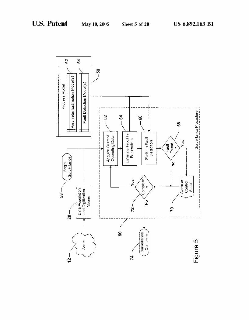
probability density function. provide an estimated value for each sensor or data signal 14 FIG. 16 illustrates an un-optimized three-term expansion of asset 12 to be monitored for the Presence of fault

probability density function model of the residual error data 40 conditions during the surveillance procedure 60. The pro- for a typical Space Shuttle Main Engine accelerometer with cess model 50 is further comprised of a fault detection model comparison to the actual residual error data and a Gaussian 54 or collection of fault detection models 54 such that at probability density function. least one fault detection model 54 is provided for each

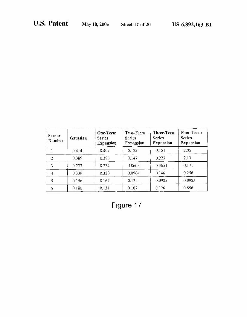
FIG. 17 lists the root mean square errors for five different sensor or data signal 14 of asset 12 to be monitored for the un-optimized probability density function models computed 45 presence of fault conditions during the surveillance proce- for each of six Space Shuttle Main Engine accelerometers dure 60. The fault detection model 54 is another hallmark of used for feasibility testing of a preferred embodiment in the instant invention and will be delineated in further detail accordance with the instant invention. hereinbelow.

FIG. 18 lists the root mean square errors for five different Process Model Training Procedure optimized probability density function models computed for SO More specifically, and referring to FIGS. 1 and 3, the each of six Space Shuttle Main Engine accelerometers used training procedure 30 of the system 10 includes a method for feasibility testing of a preferred embodiment in accor- and apparatus for training or preparing the process model 50 dance with the instant invention. using historical operating data from the asset 12 that has

FIG, 19 illustrates the optimized two-term expansion been acquired by the data acquisition means 20 using any probability density function model of the residual error data 55 combination of conventional electronic data acquisition for a typical Space Shuttle Main Engine accelerometer with hardware and signal processing software as is well known in comparison to the actual residual error data and a Gaussian the art. The historical operating data is acquired in digital probability density function. format and stored in memory means 24 using a data storage

FIG. 20 illustrates the empirical false alarm rates for Procedure 32 to create a training data set 34. feasibility testing of a preferred embodiment in accordance 60 The training data set 34 includes at least N discrete with the instant invention with comparison to the prior art Observations Of the asset l2 wherein each sing1e SPRT method. observation, herein denoted Xobs, is comprised of a vector

of data values for each signal parameter to be included in the DESCRIPTION OF PREFERRED process model 50. For the purposes of the training procedure

EMBODIMENTS 65 30, the number of observations, N, acquired is at least great Considering the drawings, wherein like reference numer- enough to adequately bound the operating state space of the

als denote like parts throughout the various drawing figures, asset 12. Thus, the training data set 34 provides a represen-

30 during the training procedure 30.

for a typical Space Shuttle Main Engine accelerometer with The system lo further a surveillance procedure wherein the stored process

comparison to the actual residual error data and a Gaussian collection of parameter estimation models 52 as necessary to

US 6,892,163 B1 9 10

tative sample of the signals produced by the asset 12 during 12 to be monitored for the presence of fault conditions all normal modes of operation. during the surveillance procedure 60. The process model

Upon acquiring the training data set 34, the unique array 50 is thereafter useful for performing surveillance of training procedure 30 can be implemented in accordance the asset 12. with instant invention. Referring to FIG. 4, the training procedure 30 is illus-

The unique training procedure 30 is comprised of a trated in additional detail. A designer 16 initializes the calibrate parameter estimator procedure 36 and a calibrate calibrate parameter estimators procedure 36 by specifying a fault detector procedure 38. The calibrate parameter estima- set of parameter estimator methods and settings 40. The tor procedure 36 creates the parameter estimation model 52 parameter estimator methods and settings 40 are then used and trains the parameter estimation model 52 using the i o to operate on the training data 34 via a nominal signal training data 34. The calibrate parameter estimator proce- behavior modeling procedure 42, for example using an dure 36 further stores this model as a new parameter MSET training procedure as described herein in detail, in estimation model 52 in the process model 50. order to create the parameter estimation models 52, which

The process model 50 may contain one or more parameter are stored in the process model 50. estimation models 52 depending upon the requirements of is Still referring to FIG. 4, the training procedure 30 next the approach taken by a designer. Continuing to refer to FIG. proceeds to the calibrate fault detectors procedure 38 3, the training procedure 30 may be, in general, performed wherein the parameter estimation models 52 are an input to using any parameter estimation method suitable for defining the procedure. The designer 16 initializes the calibrate fault a parameter estimation model 52 useful for estimating the detectors procedure 38 by specifying a set of fault detector values of one or more process signals. Methods suitable for 20 methods and settings 46. Next, the estimate process param- the calibrate parameter estimator procedure 36 include, but eters procedure 64 operates the parameter estimation models are not limited to, a plurality of redundant sensor techniques, 52 over the training data 34 to generate an estimated value a plurality of multivariate state estimation techniques, a for each monitored signal value contained in the training plurality of neural network techniques, a plurality of math- data 34. It is important that the estimate process parameters ematical model techniques, a plurality of autoregressive zs procedure 64 used in the calibrate fault detectors procedure moving average techniques, and a plurality of Kalman filter 38 be the same estimate process parameters procedure 64 techniques. Each parameter estimation model 52 contained that will later be used in the surveillance procedure 60 in the process model 50 may be created to implement any (reference FIGS. 1 and 2 for surveillance procedure 60). one of a plurality of parameter estimation techniques. Next, A compute training data residuals procedure 44 cal- Further, the parameter estimation technique implemented 30 culates the training data residuals for each monitored signal, for an individual parameter estimation model 52 is not which are calculated as the difference between the training constrained to be the same as the parameter estimation data value and the corresponding estimated data value for technique implemented for any other parameter estimation each monitored signal. The training data residuals are next model 52 contained in the process model 50. used by a compute nominal residual probability density

One example of the calibrate parameter estimator proce- 3s function (PDF) procedure 48 to create a fault detection dure 36 would be the computation of a bias term between model 54 for each monitored signal. In accordance with the two redundant sensors wherein the parameter estimation instant invention, the fault detection models 54 is typically model 52 used for estimating the value of one sensor during comprised of mathematical descriptions of the probability the surveillance procedure 60 consisted of summing the density function that best characterizes or best fits the observed value of a second redundant sensor with a bias 40 training data residual for the monitored signal. The training term computed during the training procedure 30 as the mean data is presumed to accurately characterize the expected difference between the two sensor values over the training normal operating states of the asset 12. Therefore, the data set 34. More sophisticated examples of the training training data residuals are characteristic of the expected procedure 30 using multivariate state estimation techniques normal deviations between the observed signal values and will be described herein below. 4s the values estimated using the parameter estimation models

Still referring to FIG. 3, the calibrate fault detector 52. The fault detection models 54 are stored in the process procedure 38 makes use of the parameter estimation models model 50 thereby completing the training procedure. 52 to provide estimated values for at least one signal One hallmark of the instant invention is the method and parameter contained in the training data. Generally, the system for computing the fault detection models 54 by the calibrate fault detector procedure 38 will create a separate SO means of the compute nominal residual probability density and distinct fault detection model 54 for each sensor or data function (PDF) procedure 48. As will be described math- signal of asset 12 to be monitored for the presence of fault ematically herein below, the compute nominal residual prob- conditions during the surveillance procedure 60. As delin- ability density function (PDF) procedure 48 fits a general eated infra, one hallmark of the instant invention is the fault open-ended probability function to the training data residu- detection model 54 element of the process model 50 for the ss als and employs this fitted function when implementing a asset 12 that is derived during the training procedure 30. In herein named Adaptive Sequential Probability (ASP) particular, the instant invention encompasses a statistical method and system for computing the fault detection model hypothesis test type of fault detection model 54 having novel 54 and thereafter employing said fault detection model 54 and unique characteristics and calibration procedures for the purpose of performing a fault detection procedure 66 described herein including but not limited to having a 60 of the surveillance procedure 60. probability density function model empirically derived from Surveillance Procedure a numerical analysis of asset operating data. Referring to FIG. 5, the surveillance procedure 60 is

Continuing to refer to FIG. 3, the training procedure 30 is comprised of acquiring successive vectors of current oper- completed when all training data 34 has been used to ating data and determining for each such observation vector calibrate the process model 50. At this point, the process 65 whether the current operating data is indicative of a fault or model 50 includes parameter estimation models 52 and fault failure of the asset 12. The surveillance procedure 60 further detection models 54 for each sensor or data signal of asset includes implementing an alarm or control action 70 for the

s

US 6,892,163 B1 11 12

purpose of notifying an operator and/or taking a corrective illustrated. The acquire current operating data procedure 62 action in response to a detected fault or failure of the asset is used to acquire current signal data values from signals 14 12. The surveillance procedure 60 is in general an open- monitored from asset 12 via sensors 18. The estimated value ended data acquisition and analysis loop that continues until for a first redundant sensor signal is computed using a such time as the operator chooses to terminate the surveil- s mathematical transformation on the acquired value of a lance 74. second redundant sensor signal. Said mathematical transfor-

More specifically, and referring to FIG. 5, the surveillance mation is the estimate process parameters procedure 64 that procedure 60 begins 58 with an acquire current operating in this case may be a simple equivalence or may include data procedure 62 that employs the data acquisition and biasing, de-noising or other signal processing. The compute digitization means 20 (FIG. 1) to acquire a current set of i o data residuals procedure 76 is then performed followed by signal data from the monitored asset 12. The current set of the perform ASP tests procedure 78 as described herein- signal data is provided to the estimate process parameters above and further delineated hereinbelow. procedure 64 that uses the parameter estimation models 52 Referring to FIG. 8, one possible multivariable parameter to estimate values for one or more of the current signal data estimation technique for the estimate process parameters values. The observed and estimated data are next provided is procedure 64 is illustrated. The acquire current operating to a perform fault detection procedure 66 that uses the fault data procedure 62 is used to acquire current signal data detection models 54 to determine whether a fault is found 68 values from signals 14 monitored from asset 12 via sensors in the current operating data. If a fault is found 68 is true, an 18. The estimated value for one or more sensor signals is alarm and/or control action 70 is taken. Upon completing the computed using a mathematical transformation on the fault found procedure 68, the surveillance procedure 60 then 20 acquired values of one or more sensor signals. Said math- repeats for the next available set of signal data for as long as ematical transformation is the estimate process parameters a surveillance complete decision procedure 72 determines procedure 64 that in this case may implement any feasible that additional surveillance data are available or terminates parameter estimation technique or procedure, including but at surveillance complete step 74 when no more surveillance not limited to a plurality of multivariate state estimation data are available or when terminated by an operator. zs techniques, a plurality of neural network techniques, a

Referring now to FIG. 6, the perform fault detection plurality of mathematical model techniques, and a plurality procedure 66 of surveillance procedure 60 is illustrated in of Kalman filter techniques. The compute data residuals additional detail. For each current set of signal data values procedure 76 is then performed followed by the perform acquired the estimate process parameters procedure 64 uses ASP tests procedure 78 as described hereinabove and further the parameter estimation models 52 to estimate values for 30 delineated hereinbelow. one or more of the current signal data values. The compute Referring again to FIG. 6, the usefulness of the instant data residuals procedure 76 performs a mathematical trans- invention is, inter alia, the improvement achieved in the formation on the acquired and estimated values to produce accuracy of the fault decision procedure 68 that results from a current set of residual data values. Said mathematical the improvement achieved in the accuracy of perform fault transformation is most typically a simple mathematical 3s detection procedure 66 made possible by the novel perform difference, however, any appropriate transformation may be ASP tests procedure 78 that is a hallmark of the instant used including transformations that remove correlated and invention. Improving the accuracy of the fault decision uncorrelated noise from the residual data values. The residu- procedure 68 accomplishes a reduction in the number of als produced and transformed in the compute data residuals false alarms sent to a process operator or control system that procedure 76 are next processed by a perform ASP tests 40 can in turn result in an erroneous alarm or control action by procedure 78 that uses the fault detection models 54 to the alarm or control action procedure 70. Further, improving produce a ASP fault indication that is a hallmark of the the accuracy of the fault decision procedure 68 accomplishes method and system of the instant invention. Next, the fault a reduction in the number of missed alarms thereby accom- found decision procedure 68 is performed on the basis of the plishing more timely alarm or control action by the alarm or ASP fault indication results aroduced bv the aerform ASP 4s control action arocedure 70. The instant invention therebv

, I

tests procedure 78. The fault found decision procedure 68 may have any one of a plurality of structures and procedures, including but not limited to methods and systems to perform false alarm filtering by means of observing a time series of ASP fault indication results for the purposes of determining the actual presence of a fault. In one preferred embodiment of the instant invention, a conditional probability fault found decision procedure 68 is used to perform said false alarm filtering.

Continuing to refer to FIG. 6, the estimate process parameters procedure 64 uses the parameter estimation models 52

enables improved operating safety, improved efficiency and performance, and reduced maintenance costs for a wide variety of industrial , utility, business, medical, transportation, financial, and biological processes and appa-

SO ratuses wherein such process and/or apparatus asset 12 has at least one characteristic data signal suitable for surveillance.

In use and operation, and in one preferred form, FIGS. 1 and 9 outline a general surveillance procedure of the system

ss 10 when employing the novel fault detection model 54 contained in the process model 50 and the accompanying

to estimate values for one or more of the current signal data novel fault detection procedure 66 having the perform ASP values wherein the parameter estimation method used may tests procedure 78. In a typical surveillance procedure, the have any one of a plurality of structures and procedures, asset 12 is the source of at least one process signal 14 that including but not limited to, a plurality of redundant sensor 60 is acquired and digitized using conventional data acquisition techniques, a plurality of multivariate state estimation means 20 for providing the data acquisition procedure for techniques, a plurality of neural network techniques, a the purpose of computer-assisted surveillance. The digitized plurality of mathematical model techniques, a plurality of signal data is generally evaluated using a computer 22 autoregressive moving average techniques, and a plurality of having computer software modules implementing the esti- Kalman filter techniques. 65 mate process parameters procedure 64, and the perform fault

Referring to FIG. 7, one possible redundant sensor tech- detection procedure 66. The estimate process parameters nique for the estimate process parameters procedure 64 is procedure 64 is used to produce an estimated signal value for

rithm that uses advanced pattern recognition techniques to measure the similarity or overlap between signals within a defined domain of asset operation (set of asset operating 35

- D =

d2,i 4 2 . . . d2,m - - .... .... = [ X ( r , ) , X(r21 , ... , ;(rm)] ....

US 6,892,163 B1 15 16

memory matrix. To obtain the weight vector, we minimize the error vector, R, where:

incorporated herein by reference in its entirety. The SPRT analyzes a sequence of discrete residual error values from a signal to determine whether the sequence is consistent with normal signal behavior or with some other abnormal behav-

s ior. When the SPRT reaches a decision about the current signal behavior, e.g., that the signal is behaving normally or abnormally, the decision is reported and the test continues analyzing the signal data. For any SPRT, signal behavior is

(E4) - - - R = X obs- est

The error is minimized for a given state when:

G = ( B Q 1)-1.( B@ ZObJ (Es)

This equation represents a “least squares” minimization when the pattern recognition operator @ is the matrix dot product. Several advanced pattern recognition operators have been defined that provide excellent parameter estimation performance. Pattern recognition operators used by MSET include, but are not limited to, the System State Analyzer (SSA) method (see also U.S. Pat. No. 4,937,763 which is hereby incorporated by reference in its entirety), the Bounded Angle Ratio Test (BART) method (see also U.S. Pat. No. 5,987,399 which is hereby incorporated by reference in its entirety), the Vector Pattern Recognizer (VPR) method, the Vector Similarity Evaluation Technique (VSET) method, and the Probabilistic State Estimation Method (PSEM).

Once the weight vector is found, the resulting current state estimate of the system (i.e., the parameter estimate vector) is given by;

The first application of the pattern recognition operator in equation E6 (DT@ D) involves a comparison between the

10

1s

20

2s

30

defined to be normal when the- signal’data adheres to a Gaussian probability density function (PDF) with mean 0 and variance 0’. Normal signal behavior is referred to as the null hypothesis, H,. MSET employs four specific SPRT hypothesis tests. Each test determines whether current signal behavior is consistent with the null hypothesis or one of four alternative hypotheses. The four tests are known as the positive mean test, the negative mean test, the nominal variance test, and the inverse variance test. For the positive mean test, the corresponding alternative hypothesis, H,, is that the signal data adhere to a Gaussian PDF with mean +M and variance 0,. For the negative mean test, the corresponding alternative hypothesis, H,, is that the signal data adheres to a Gaussian PDF with mean -M and variance 0’. For the nominal variance test, the corresponding alternative hypothesis, H,, is that the signal data adheres to a Gaussian PDF with mean 0 and variance Va2. For the inverse variance test, the corresponding alternative hypothesis, H,, is that the signal data adheres to a Gaussian PDF with mean 0 and variance */V. The user-assigned constants M and V control the sensitivity of the tests. Limitations of the SPRT Fault Detector Training and Sur-

row vectors in theDT matrix and each of the column vectors veillance Method and System in the D matrix. If we define G=DT@D, then G, the One significant shortcoming of the SPRT technique is similarity matrix, is an m by m matrix. The element in the found in the assumptions underlying its mathematical for- i-th row and j-th column of the matrix (gJ represents a mulation. Specifically, the SPRT technique presumes that measure of the similarity between the i-th and j-th column 35 the residual error signals adhere to a Gaussian probability vectors (i.e., memorized states) in the process memory matrix. The second application of the pattern recognition operator in equation E6 (DT@X,,) involves a comparison between the row vectors in the DT matrix and each of the elements in the observation vector Xobs. If we define A=DT@X,,, then A, the similarity vector, is an m by 1 vector. Each element in the similarity vector is a measure of the similarity between the observation vector and the i-th column vector (i.e., memorized state) in the process memory matrix.

density function. For residual error signals that are non- Gaussian, the fault detector false alarm rates and/or missed alarm rates specified by the designer are not accomplished by the SPRT procedure thereby degrading the fault decision

40 accuracy of the asset control and/or surveillance system. The novel ASP technique of the instant invention specifically removes the assumption that the residual error signals adhere to a Gaussian probability density function. The ASP technique implements any one of a plurality of methods to

4s numericallv fit a arobabilitv densitv function to the observed , I

Note that the similarity matrix is a function of the process residual error signal distribution that is characteristic of memory matrix only. Thus, the similarity matrix and its normal asset operation. The derived probability density inverse Ginv=(DT@D)-’ can be calculated as soon as the function is then used to perform a dynamic statistical process memory matrix has been derived thereby making the hypothesis test thereby achieving the fault detector false application of MSET to an on-line surveillance system more SO alarm and missed alarm rates specified by the designer and computationally efficient. Computation of the Ginv matrix improving the fault decision accuracy of the asset control initializes the parameter estimation model and completes the and/or surveillance system. second of three steps in the procedure for training an MSET Fault Detection Using Statistical Hypothesis Test Proce- model based on historical operating data. dures

The general theory underlying the statistical hypothesis includes analyzing the historical training data using equation test will now be delineated below. Next, the SPRT imple- E4 to produce a residual error vector, R, for each observation mentation of a dynamic statistical hypothesis test will be vector in the training data. The collection of residual error described. Finally, the novel ASP implementation of a vectors comprises the training data residuals necessary for dynamic statistical hypothesis test for non-Gaussian residual training the fault detection model 54 using any one of a 60 error signals will be delineated in detail along with a plurality of techniques, including but not limited to the delineation of its reduction to practice. SPRT technique, and the novel ASP technique that is a Bayes’ Rule for a Single Observation hallmark of the instant invention. Statistical decision problems in which there are just two

The Sequential Probability Ratio Test (SPRT) technique is possible outcomes constitute an important class called a statistical hypothesis test fault detection algorithm histori- 65 binary hypothesis testing problems. The possible states of a cally used for MSET process surveillance. The SPRT tech- system are called hypotheses and each individual state of the nique is described in U.S. Pat. No. 5,459,675, which is system is termed a simple hypothesis. A simple hypothesis

The third and final step in the MSET training procedure ss

US 6,892,163 B1 17 18

is a complete specification of a probability distribution for the system (i.e., the distribution of possible observations or samples from the system). The “hypothesis” being tested is that the particular distribution is the correct one.

The basic operation in a binary hypothesis test is to 5 evaluate the veracity of a hypothesis, H, given a piece of

Because of the unpredictability or element of chance inher- ent in the system, the test deals with the probabilities that events occur or that hypotheses are true. The probability that a hypothesis is true given a piece of evidence is written as P(H1e). The notation identifies a conditional probability- namely the probability that the hypothesis is true under the condition that the event has occurred with absolute certainty.

listic Reasoning in Intelligent Systems: Networks of Plau- sible Inference, by Judea Pearl, Morgan Kaufmann Publishers, Inc., San Mateo, Calif., 1988, Second Edition at pages 29 through 39, provides a means for evaluating the conditional probability of a hypothesis, P(Hle), which is also

The complementary form of Bayes’ rule provides the posterior probability for the converse of the hypothesis. It is evaluated by substituting for each instance of H in equation E l l and noting that -(-H)=H:

P(el7 H ) P ( 7 H ) (E121 P(7 Hle) = evidence or observation, e, from the system being studied. P ( e I H ) P ( H ) + P(el7 H ) P ( 7 H ) ’

alternate form of &yes’ rule is produced by dividing it (i,e,, equation E l l ) with its complementary form (i,e,, equation 132) to obtain

(~13) P(Hle) - P(elH) P ( z ) Bayes’ well known inversion rule, as described in Probabi- ~ ~~

~ ( 7 Hie) - P(el7 H ) ~ ( 7 H ) ’

This form of Bayes’ rule is further manipulated by first defining the prior odds on hypothesis as

known as the posterior probability,

P(eIff)P(H) ’

P(Hle) = ~

the likelihood ratio as 2s

P(e1H) is the probability that the observation would occur

hypothesis is true before any observations of the system have been made. also known as the arior arobabilitv. The

P(elH) if the hypothesis is true. P(H) is the probability that the L(elH) = ~ P(el7 H)’

I I

denominator, P(e), is the unconditional probability that the 3o observation occurs. and the posterior odds on H as

Basic axioms of set theory can be used to prove the

,S), where -S is the converse of event S. In probability P(Hle)

P(7 Hie) following identity for two events R and S: R=(RflS)U(Rf’ O(Hle) = ~

theory, the analog of this identity is P(R)=P(R, S)+P(R, Ts),

3s Bayes’ rule then specifies the posterior odds as the

product of the likelihood ratio and the prior odds,

where the notation P(R,S) is used represent the probabil- O(f4e)=L(~lH)~(H). (E171

ity of the joint event RflS. The multiplication law states 40 that the probability of two events occurring jointly can be expressed as a function of the conditional probability of one event based on the other,

Baves’ The formulation above Specifies Bayes’ rule for a Single

observation and a binary hypothesis. For the application of binary hypothesis tests to real world signals, the formulation

( ~ 9 ) 4s must be able to handle a sequence of discrete observations. This is accomplished by beginning with a single observation and successively updating Bayes’ rule for each successive

for a Time Series

P(R, S)=P(R IS)P(R).

If and are independent events, then P(R~S)=P(R) and the multiplication law simplifies to P(R, S)=P(R) P(S).

&yes’ rule can be simplified by eliminating the denominator in equation E7, Combining equations E8 and E9, and

observation. Let the sequence cy,) be an Ordered set Of

{yfi)=Y1, Y2, ’ ’ ’ 3 Yfi? in which the are

substituting e for and written as

for s, the denominator can be so observations of the signal made at n discrete moments in time such that tlet2e . . . et,. Bayes’ rule for the first observation (yl) in the time series is

p(e)=P(eIH)P(H)+P(eI-H)P(lH). (E10)

Therefore, Bayes’ rule becomes

(Ell) Adding the second observation from the time series,

Bayes’ rule for the joint event ylfly2 is

The power of Bayesian techniques comes primarily from 60

local, namely, given that H is true, the probability of e can be estimated naturally and is not dependent on many other propositions. For instance, given that the measurements With the aid of the multiplication law (equation E9), the from an experiment adhere to a particular PDF, the prob- 65 joint event probabilities are converted to conditional probability that any single measurement will occur is easily abilities so that the right hand side of this equation can be computed rewritten as

R Y l , Y21fmH) P ( Y l r Y 2 ) ’

(E191 the fact that in causal reasoning the relationship P(e1H) is P(HlY1, Y 2 ) =

US 6,892,163 B1 19

Note that the probability of the joint event y1?y2 is written as P(y,, y,)=P(y,ly,) P(yl) instead of the equivalent P(y,, y,)=P(y,, y2) P(yJ because of the temporal dependency of the data. The second form of the multiplication law reduces to P(y,, y2)=P(y1) P(y,) because earlier events (e.g., y,) in a time series cannot be dependent on later events (e.g.,

The multiplication law is used for each successive observation in the time series to derive the form of Bayes’ rule for the joint event (ylny2n . . . fly,):

RHlYl, Y Z r ... 1 Y n ) =

Y2).

(E211

Since the probabilities for each of the later observations in the time series are conditioned on earlier observations, Bayes’ rule is difficult to solve in the general case. But if the observations in the series are independent of each other (i.e., random), then the probabilities will be dependent on the hypothesis only. In this case the conditional probability for the ith observation, P(y,ly,-,, . . . , y,, H), is simply P(y,lH). Thus, Bayes’ rule for independent observations in a time series is

If an explicit time dependency can be established for the observations in the time series (i.e., a function is found that relates earlier events to later events), then the general form of Bayes’ rule (equation E21) can be used to develop failure detection models for serially-correlated signals. However, the residual signals formed by the difference between the observed and estimated signal values are in general random signals; thus, Bayes’ rule for random time series is used as the basis for the fault detection models.

Dividing by the complementary form of Bayes’ rule for random time series and utilizing the definition of the posterior odds, prior odds, and likelihood ratio from above, an alternate form of Bayes’ rule for a time series is developed:

If we take the logarithm of this equation, the incremental nature of Bayesian formulation becomes more apparent. Equation E24 shows the log of the likelihood ratio as a weight, carried by each observation in the sequence, which additively sways the belief in the hypothesis one way or the other.

Sequential Hypothesis Tests Wald first presented and studied the following sequential

test of a simple hypothesis against a simple alternative, as

20 described in Sequential Analysis, by A. Wald, John Wiley and Sons, Inc., New York, 1947. Let H, be a specific probability density function called the null hypothesis. Then the probability that the time series CY,} contains samples

s drawn from H, is P(y,, y2, . . . , ynlHo). Let H, be a different probability density function called the alternative hypothesis. Then the probability that the time series {Y,} contains samples drawn from H, is P(y,, y2, . . . , y,lH,). Two threshold limits A and B are chosen, with A<B, and after

i o each observation in the series the following statistic (A,,,) is calculated:

1s

The test procedure is then as follows. If the statistic is greater than or equal to the upper threshold limit (i.e., Aj,,2B), then a decision is made to accept hypothesis H, as

2o true. If the statistic is less than or equal to the lower threshold limit (i.e., A,,,SA), then a decision is made to accept hypothesis H, as true. If the statistic falls between the two limits (i.e., A<A,,,<B), then neither hypothesis can yet be accepted to be true and sampling continues. If the

2s observations in the series are independent random variables, then the test statistic reduces to a product of conditional probabilities:

In the sequential hypothesis tests, the logarithm of the test statistic is often easier to work with:

3s

40 The sequential hypothesis test consists of calculating the logarithm of the test statistic for each observation in the series and comparing the result to the logarithms of the lower and upper threshold limits.

The statistic in the sequential hypothesis test is a product 45 of a sequence of likelihood ratios. Each term in the product

is the ratio of a probability conditioned on one hypothesis to a probability conditioned on a second hypothesis. The difference between the likelihood ratios in the sequential hypothesis tests and those in Bayes’ rule (see equations E15

50 and E23), is that in Bayes’ rule the probabilities are conditioned on a hypothesis and its converse, whereas in the sequential hypothesis tests the probabilities are conditioned on two hypotheses from a set of related hypotheses. In principle, the two hypotheses in the sequential hypothesis

5s tests could be the converse of each other (i.e., the set contains two elements), but in practice the hypotheses are selected from an infinite set of exhaustive and mutually exclusive hypotheses. For instance, suppose the null hypothesis is a Gaussian PDF with a mean of 1 and a variance 10.

60 Then a sequential hypothesis test can be defined in which the alternate hypothesis is any Gaussian PDF in which the mean is not 1 and/or the variance is not 10.

It is informative to compare the sequential hypothesis tests to Bayes’ rule for a time series. Given a null hypothesis

6s H, and an alternative hypothesis H,, the likelihood ratio for an observation e conditioned on the two hypotheses is defined as

US 6,892,163 B1 21

The subscripts emphasize the fact that the two hypotheses are selected from an infinite set of related hypotheses. The prior odds for the two hypotheses are defined as

while the posterior odds are defined as

Assuming the observations in the time series are independent, then Bayes' rule conditioned on hypothesis H, (i.e., equation E22 with the symbol H replaced by H,) can be divided by Bayes' rule conditioned on hypothesis H, to produce Bayes' rule for a sequential hypothesis test:

Dividing this equation through by the prior odds, it becomes apparent that the statistic in the sequential hypothesis test is just the ratio of the posterior odds to the prior odds:

The prior odds are the ratio of the probability that the alternative hypothesis is true to the probability that the null hypothesis is true, before any data have been collected from the system. In many cases, these probabilities are not known-no prior information about the system is known. In the absence of prior information about the system, these probabilities are taken to be %, making the prior odds equal to 1. Thus in the absence of prior information, the test statistic is equal to the odds that the system adheres to the alternative PDF as opposed to the null PDF. Error Probabilities for the Sequential Hypothesis Tests

Because the sequential hypothesis tests make decisions based on probabilities, there is always a finite probability that a decision reached by the test is erroneous. If a sequential hypothesis test makes a decision to accept the alternative hypothesis H, as true when the null hypothesis H, is true, then an error of type I is said to have occurred. If a sequential hypothesis test makes a decision to accept the null hypothesis H, as true when the alternative hypothesis H, is true, then an error of type I1 is said to have occurred. Although the designation is arbitrary, it stems from situations in which one kind of error is more serious than the other. Since the normal usage of the sequential hypothesis tests is to detect a change in signal response from its normal behavior (i.e., hypothesis H,) to some abnormal behavior (i.e., hypothesis H,), the error of accepting H, when H, is true is the more serious error. The probability that a decision to accept hypothesis H, is erroneous is denoted by a. A type I decision error is also called a false alarm and the probability of a type I error is called the false alarm probability. The probability that a

S

10

1s

20

2s

30

3s

40

4s

so

5s

60

65

22 decision to accept hypothesis H, is erroneous is denoted by 0. A type I1 decision error is also called a missed alarm and the probability of a type I1 error is called the missed alarm probability.

The sequential hypothesis tests are open-ended. The tests will continue to collect observations from the system and update the test statistic until the test statistic satisfies one of the two decision conditions. In principle, the number of observations needed to reach a decision can be any positive integer, although it can be shown that a decision will be reached in a finite number of observations. Since the number of observations needed to make a decision is indeterminate, the probability that a decision is erroneous is found by summing the probability of an erroneous decision being made after 1 observation, 2 observations, and so on. Formally, in terms of the threshold limits A and B that define the test, the false alarm probability is given by:

.=P(A,,,>BIH,)+P(B<A,,,<A, A,,,2BIHo)+ . . . (E331

The first term in the sum is the probability that the test statistic drops below the lower threshold limit after only one observation given that the alternative hypothesis is true. The second term is the probability that the test statistic drops below the lower threshold limit after two observations given that the alternative hypothesis is true. Similarly, the missed alarm probability is given by:

fi=P(A,,, %IH,)+P(B<A,,,<A, A,,,<AIH,)+ . . . (E341

These expressions are by no means easily computed. Moreover, one could not hope to solve these equations for A and B in terms of given a and 0, despite the desirability of being able to do so in setting up a test to provide a specified protection. Although these equations cannot be solved, it can be shown that the error probabilities and the threshold limits are related by the following inequalities

E 1 8 (E33 A > - (1-P) and p > h

The error probabilities and the threshold limits are related by inequalities because the test statistic does not usually attain exactly the value A or the value B when the test is completed. But since a decision is declared as soon as an observation drives the test statistic past either threshold, the inequalities are almost equalities. Indeed, in practice, A and B are taken to be equal to a/(l-0) and (l-a)/o, respectively. Doing so, of course, means that the sequential hypothesis test actually carried out has error probabilities that are somewhat different than those specified. Let a' and 0' denote the empirical error probabilities actually attained by a test using specified threshold limits of A=a/(l-o) and B=(l-a)/ 0. Then according to the inequalities in equation E35, the empirical error probabilities (i.e., a' and 0') are related to the preassigned error probabilities (i.e., the values of a and 0 used to specify the threshold limits) by

Multiplying these through to eliminate denominators, one obtains

US 6,892,163 B1 23 24

Adding these two equations together, one obtains an inequality relating the empirical error probabilities to the

~ ( y ; ~ , $ ) = ~ e x p - ~ ( ~ - ~ ) ~ , l l ' I preassigned error probabilities: C Y 5

(E38) 5 for which the mean (p) is 0 and the variance is 2. Thus, the

One of the key features of the hypothesis test technique is that the designer can specify the error probabilities. This is

probability that a discrete Observation ( Y d hypothesis is expressed as occurs given the

particularly important for type I errors, because false alarms ~(Y,l~d=N(Y,; 0, 03. (E411

typically do not lead to incorrect decisions, This is The four SPRT tests historically used with MSET are the because in the event that a real failure does occur, missed Positive mean test, the negative mean test, the nominal alarms may delay the time to detect the failure but not the variance test, and the inverse variance test. For the positive ability to detect the failure. The result above (equation E38) mean test, the corresponding hypothesis, H ~ , is shows that the preassigned false alarm probability is not a IS that the signal data adhere to a Gaussian PDF with mean +M strict upper limit for the empirical false alarm probability. and variance 2, where M is the Preassigned system distur- Similarly, the preassigned missed alarm probability is not a bance magnitude for the mean test. For the negative mean strict upper limit for the empirical missed alarm probability, test, the corresponding alternative hypothesis, H,, is that the even when the hypothesis test is applied to purely random signal data adheres to a Gaussian PDF with mean -M and data. It is the sum of the preassigned error probabilities that 2o variance 2. Referring to FIG. 10, the hypotheses for the two is an upper limit for the sum of the empirical prob- mean tests are illustrated for M=2 and a2=1. For the nominal abilities, Thus it is possible with purely random data for one variance test, the alternative hypothesis, H,, is that the signal of the empirical error probabilities to exceed its correspond- data adheres to a Gaussian PDF with mean 0 and variance

probabilities cannot be greater than their corresponding 2s nitude for the variance test. For the inverse variance test, the preassigned error probab corresponding alternative hypothesis, H,, is that the signal

data adheres to a Gaussian PDF with mean 0 and variance a'N. Referring to FIG. 11, the hypotheses for the two can be determined from the inequalities in equation E36, variance tests are illustrated for V=2 and a2=1. The condi-

30 tional probabilities that a discrete observation (yl) occurs E ' r - < u a n d p ' r - < - B P (E39) given one of the four alternative hypotheses are expressed as

can cause an operator to make an incorrect decision. Type I1 Io

ing preassigned error probability, but both empirical error Va2, where v is the Preassigned system disturbance mag-

True upper bounds for the empirical error probabilities

E'

(1 -PI - (1 -PI (1 - E ' ) - (1 - E ) '

fly, I Y) = N(Y,; M , $1,

fly, I f f 3 ) = N(y,; 0, V d ,

( ~ 4 2 )

For small preassigned error probab fly, I H z ) =N(Y,; - M , $1, bounds are only slightly greater than the preassigned error 35

probabilities are 0.01 then the empirical error probabilities of the test will not exceed 0.0101. The Sequential Probability Ratio Test (SPRT)

es. For instance, if both of the preassigned error

40 The sequential hypothesis tests described herein above are

eses, MSET has historically employed four specific sequential hypothesis tests to detect signal faults. These four tests

general statistical tests valid for any pair of related hypoth- The logarithm of the test statistic for the four SPRT tests can be evaluated by substituting the conditional probabilities from equations E41 and E42 into the genera'

are called the Seauential Probabilitv Ratio Tests. or SPRTs, ~~ (equation E27) and Thus, for the positive mean Ti

The SPRTs moniior for changes in'the statistical characteristics of the residual signals. A residual signal is the difference between an actual signal and MSET's estimate of that

generating sequences of decisions. A decision in which the so null hypothesis is accepted (i.e., A,,,SA) is called a normal decision and implies that the residual signal is behaving as anticipated. A decision in which the alternative hypothesis is accepted (i.e., A,,,ZB) is called a fault decision and implies that the residual signal is behaving abnormally.

test,

In = 2 In[N(Y1; M , $11 signal. The SPRTs continually monitor a residual signal, N(y,; 0, u 2 )

,=I

1 exp [ --( zu2 y1 - M ) 2 )

= 2 hy2) = 2 Y? - (Y! - M I 2 55

The null hypothesis upon which the SPRTs are based specifies that the residual signal consists of Gaussian data

2u2 ,=I

that have a sample mean of 0 and a sample variance of a,. M " M 2

= -E (y! - -) SPRT,,. 2u2 ,=I

A training procedure, during which the system is operating normally, is used to verify that the mean of the signal is 0 and 60 to evaluate the variance of the signal. Note that if the residual signal does not have a mean of 0, the calculated The equation E43 defines the SPRT index for the positive mean from the training phase is used to normalize the mean test (SPRT,,). ASPRT index is defined for each of the residual signal for the surveillance procedure using the four sequential hypothesis tests. The SPRT indices are the model. Thus the null hypothesis, H,, for the SPRTs is that 65 actual quantities computed by the SPRT fault detection the signal being analyzed adheres to Gaussian PDF (N(y; p, procedure. The SPRT index for the negative mean test a2h (SPRT,,,) is given by

US 6,892,163 B1 25 26

the SPRT technique to non-Gaussian PDFs. In the ASP method, the assumption that the data fit a Gaussian PDF is relaxed and the test statistic is evaluated for any arbitrary data distribution. In the ASP method, the signal is assumed to consist of random observations that adhere to a specific PDF that is a function of the sample mean, variance, and possibly higher order terms. The PDF is denoted by the

2 ln[ N(Y,; -M, $11 (E441 In A2,n =

N(y,; 0, u 2 ) ,=I

M " M

2u2 ,=I 2 = -E (-y! - -) =SPRTne8.

= 2 1 n

,=I

general function S(y; p, 2, . . . ). The parameter list of the function is open-ended to indicate that additional terms, such as the sample skewness, kurtosis, or width of the

The SPRT index for the nominal variance test (SPRT,,,) is given by

1 - & & x p 4 a

1 Y: s e x p ( - P l

specifies that the data distribution has a sample mean of 0 and a sample variance of 3. A training phase, during which the system is operating normally, is used to verify that the mean of the signal is 0 and to evaluate the sample variance.

~

butions that are typical for residual error signals produced by parameter estimation based techniques, such as MSET. The logarithm of the test statistic for the four ASP tests Mathematical Foundations of the ASP Test can be evaluated by substituting the conditional probabilities

The Adaptive Sequential probability (ASP) method from equations E47 and E48 into the general formula defines four new sequential hypothesis tests. The Adaptive 65 (equation E27). The logarithm ofthe test statistic for a given Sequential Probability method is an advanced failure detec- test is defined to be the ASP index for that test. The ASP tion technique that broadens the domain of applicability of index for the positive mean test (ASP,,,) is given by

US 6,892,163 B3 27 28

where the standard normal PDF

The ASP index for the negative mean test (ASP,,,) is given by

The ASP index for the nominal variance test (ASP,,) is given by

The ASP index for the inverse variance test (ASPi,,) is given by

The ASP tests are then implemented in the same manner as the SPRT tests. Namely, for each time step in the calculation, the four ASP indices are calculated (equations E49 through E52). Each ASP index is compared to the upper and lower log-thresholds and the status of the test is evaluated (i.e., faulted, normal, or continuing). ASP Method for Near-Gaussian Distributions

The Adaptive Sequential Probability method consists of four specific sequential hypothesis tests applied to non- Gaussian data distributions. In order to use the method, a general PDF, S(y; p, 02, . . . ), must be defined for the target signal. In this section, the ASP method is derived for data distributions that are nearly Gaussian.

In applications of MSET to the Space Shuttle Main Engine accelerometer signals, applicants discovered that the residual signals produced by the system model have a nearly, but not truly, Gaussian behavior, as described in Dynamics Sensor Data Validation Phase I Final Report, by applicants: Randall L. Bickford and James P. Herzog, NASA Contract NAS8-40874, Jul. 1,1997. When plotted as a histogram, the residual data will appear to have the same bell-curve shape as a Gaussian distribution. But when a Gaussian PDF of the same mean, standard deviation, and area as the data distribution is superimposed on it, the histogram was found by applicants to be non-Gaussian. Typically, applicants found that the histogram has thicker tails than the Gaussian curve, which corresponds to a sample kurtosis that is greater than 3.

A PDF can be written as a sum of a standard normal distribution, Z(x), and a remainder term, R(x), as described in Mathematical Methods of Statistics, by H. Cramer, Prin- ceton University Press, Princeton, N.J., 1946.

30

3 s

40

4s

so

55

60

65

is a function of the dimensionless variable x=(y-p)/o. The standard normal PDF is related to the general Gaussian PDF (equation E40) through the normalization condition:

The remainder term can be expressed as an infinite series of orthogonal polynomials whose terms are functions of derivatives of the standard normal PDF. The constant coefficients of the polynomial terms are dependent on the central moments of the target distribution. As described in Hand- book of Mathematical Functions, by M. Abramowitz and I. A. Stegun, Dover Publications, Inc., New York, 1972, the first four terms in the series expansion of the remainder function are:

The pi factors are central moments of the discrete data sequence CY,)=(y,, y2, . . . , Y,),

1 " 1 "

J=I lz ,=I pI = ; z ( y J - p ) I with p = - C y J and

The Z(")(x) functions are derivatives of the standard normal PDF. The nth derivative of the standard normal PDF is given by:

where He,(x) are the Hermite polynomials. The first twelve Hermite polynomials are

He,(x)=x:

He2(x)=x2- 1,

He3(x)=x3-3x,

He4(x)=x4- 6x2+3,

He,(x)=&10x3+1Sx,

US 6,892,163 B1

Application of the ASP Method to Space Shuttle Main Engine Residual Signals

In one application use and operation, and in one preferred embodiment, the ASP technique was reduced to practice to

10 provide highly reliable data validation for high frequency Space Shuttle Main Engine (SSME) accelerometers. Each

accelerometers with three sensors mounted on each of the two high pressure turbopumps and two sensors mounted on

Helo(x)-x10-4Sx8+630x6-31SOx4+472Sxz-94S,

Hell(x)=x11-SSx9+990x7-6930?+1732Sx3-1039Sx,

~ ~ l z ( ~ ) ~ ~ 1 z - ~ ~ ~ 1 o + ~ ~ ~ ~ ~ 8 - ~ ~ ~ ~ ~ ~ 6 + ~ ~ ~ ~ ~ ~ 4 - ~ ~ ~ ~ ~ ~ z + ~ ~ ~ ~ ~ ~ ~ ) SSME is monitored by eight high frequency kHz)

Each term in the series expansion of the remainder function R(x) is more complex than the previous term as 1s the engine gimbal higher central moments of the data distribution and higher

MSET were the Asp method for the six turbopump prepared to

accelerometers. The MSET pattern recognition algorithm derivatives of the standard normal PDF are introduced. The produces extremely accurate simulations of turbopump nth term in the remainder function depends on the central accelerometer behavior. Referring to FIG. 12, some results moments from order 1 (i.e., mean) through order n+2. Thus, from applying the six sensor MSET model to a typical Space the first term depends on moments through the third central 20 Shuttle flight (i.e., flight STS057, engine 1) are shown. For moment (i.e., skewness), the second term depends on the calculation shown in FIG. 12, the MSET training algo- moments through the fourth central moment (i.e., kurtosis), rithm extracted a small fraction of the data in the acceler- and so on. ometer signals to simulate the behavior of the accelerom- If the data distribution that is to be approximated with eters (the process memory matrix contained only o,oo83%

be achieved with only a few of the terms in the series. In the signal from the first SSME turbopump accelerometer in the ASP method for near-Gaussian distributions, the data dis- model (i,e,, the oxidizer preburner pump 45 accelerometer) tribution is first approximated with the standard normal PDF, is shown as a function of time from the launch of the Space

higher terms of the remainder function until an adequate fit 30 erometer signal shows the very high accuracy of the MSET

produced. In practice it is usually not advisable to go beyond the difference between the signal and MSET's esti- the fourth term in the remainder function because the tail mate of that signal, is shown in the bottom plot, The relative

error in the calculation, as measured by the ratio of the regions of the general PDF become unstable. Using the equations for the derivatives of the standard 3s standard deviation of the residual signal to the standard

normal PDF (equations E59 and E5912 the remainder fmc- deviation of the sensor signal, is only 0.86%. The results tion can be written as a product of the standard normal PDF shown in FIG, 12 illustrate MSET~ ability to accurately and a polynomial whose coefficients depend on the central model highly dynamic signals, even when only a tiny moments of the data distribution. fraction of available data is used to represent the signal

behavior. Still referring to FIG. 12, the residual signal for the

analysis of a typical SSME accelerometer appears to be random. Referring to FIG. 13, the distribution of data in the residual signal is shown. The probability density for the residual signal was approximated by dividing the data range into m equally-sized bins and then counting the number of residual signal data values that fall into each bin. The count number is a discrete function of the sequence {Y,}=yl, y2, . . . , y,, where the ith element in the sequence (yl) is

equation E53 is nearly Gaussian, a good approximation will 2s of the raw signal data), In the top plot, the highly dynamic

'('1. The approximation is refined by adding successively Shuttle, In the middle plot, MSET's estimate of the accel-

between the general PDF, s(x), and the data distribution is simulation, The residual signal for the calculation, which is

40

(E601 R(x) = Z ( x ) C rI (XI.

,=I

4s where the first four terms in the series are

(E61)

(E62) given by

1 P3 rl

r2(x) = -(- 1 P4 -3)He4(x)+ -(?) 1 P3 2 H, , (x) ,

= - 6 - u 3 He3 (XI.

24 d 72 u

5s 1 P3 P4 1 P3 3 --(- 1 u U 3 d -3)He,(x)+ m(p) He,(x) ,

and ymin is the minimum datum and y,, is the maximum datum in the residual signal. A normalized residual signal

720 u6 d u3 PDF is produced by dividing each element in the count -(- 1 P4 -3) 3 H e , ( x ) + number function by the total number of elements in the 1152 d 60 residual signal. The number of bins used to produce the

residual signal PDFs was 1000. As shown in FIG. 13, a PDF for a typical residual signal has a nearly Gaussian shape. Superimposed on top of residual signal PDF is a Gaussian PDF of the same mean, standard deviation, and area as the

65 residual signal PDF. The first four moments of the residual signal data are as follows: m e a ~ ~ = l . l * l O - ~ g, standard deviation=8.2* lo-' g, skewness=0.32, and kurtosis=5.7,

r4(x) = -( - P6 - 1 5 ' 4 - 10( E)' + 30)He,(x) + (E641

"( '5 - lO")H,, (x) + 7 2 0 ~ 3 us u 3

1 P 3 2 W 1 P3 4 -(-) 1728 u3 (7 -3)~e , , (x)+ 311O4(p) ~ e 1 2 ( x ) .

Thus, the series expansion formula for the approximation of the general PDF is

US 6,892,163 B1 31

where the skewness and kurtosis are related to the third and fourth central moments of the data by

Because the kurtosis of the distribution is greater than 3, the residual signal PDF has thicker tail regions than a true Gaussian distribution. This is confirmed by a visual exami- nation of FIG. 13.

The ASP method for near-Gaussian distributions was applied to the residual signals from the MSET model of the SSME accelerometers. The residual signal PDFs were approximated with the series expansion formula of a general PDF (equations E60 through E65). Four calculations were performed for each residual signal in the model. In the first calculation, the residual signals were approximated with the one-term series expansion formula. In the one-term formula, the remainder function (R(x)) is given by the product of the standard normal PDF and the first term in the series, rl(x). Subsequent calculations introduced additional terms from the series, culminating with the four-term formula in which the remainder function is given by the product of the standard normal PDF and the four term series, r1(x)+r2(x)+

For each calculation, the quality of the approximation is measured by the root mean-squared (rms) error of the calculation. The rms error (Ems) is a function of the difference between the calculated PDF @(.)) from equation E65 and the residual signal PDF (F(x)),

r3(x)+r4(x).

The calculated and residual signal PDFs are discrete functions of the dimensionless variable xi=(yl-p)/a, where y1 is an element in the sequence that spans the range of data in the residual signal distribution (see equation E66).

In general terms, each additional term in the series expansion improves the approximation of the residual signal PDFs. Referring to FIG. 14, FIG. 15 and FIG. 16, adding terms from the series expansion formula improves the fit of the residual signal PDF from the first sensor. The approximation of the residual signal PDF generated by the one-term series expansion formula is compared to a Gaussian approximation and the residual signal PDF in FIG. 14. The one-term approximation shows little improvement over the Gaussian approximation. The rms error for the Gaussian PDF is 0.414, while the rms error for the one-term series expansion PDF is slightly smaller at 0.409. The PDF generated by the two-term series expansion formula is shown in FIG. 15. The fit of the two-tern approximation is significantly better than that of the Gaussian approximation. The two-term formula provides an excellent fit of the residual signal PDF, espe- cially near the peak in the distribution. The greatest source of error in the approximation occurs in the transition regions of the distribution, between 1 and 4 standard deviations from the mean. The rms error for the two-term series expansion PDF is 0.122, which is nearly a factor of four smaller than the rms error of the Gaussian PDF. The PDF generated by the three-term series expansion formula is shown in FIG. 16. The three-term formula provides a better fit of the peak in the distribution than does the two-term formula. The rms error for the three-term approximation is 0.151, which is slightly larger than that of the two-term approximation because its fit of the lower transition region is less accurate than that of the two-term approximation.

32 The rms errors of the four calculations for each of the

sensors in the model are listed in FIG. 17. Also included in FIG. 17 are the rms errors for Gaussian PDFs of the same mean, standard deviation, and area as the residual signal

s PDFs. As indicated by the data in the first two columns of FIG. 17, the one-term series expansion formula produces PDFs that are slightly more accurate than the corresponding Gaussian PDFs. Significant improvement is exhibited by the two-term series expansion formula, which produces PDFs

i o whose rms errors are as much as a factor of four smaller than those from the corresponding Gaussian and one-term series expansion approximations. The three-term series expansion formula generally produces larger rms errors than does the two-term formula because the fit of the transitions regions of

is the distribution is less accurate. This trend is further exhibited by the four-term series expansion formula. For three of the calculations (i.e., sensor numbers 1, 2, and 6), the four-term approximations are unstable in the transition regions, resulting in rms errors that are much larger than

20 those of the corresponding Gaussian approximations. The four-term series expansion formula produces an improved approximation for the residual signal from sensor number 5 only. The residual signal for this accelerometer is the most nearly Gaussian of the sensors to begin with, as indicated by

zs the rms errors for the Gaussian approximations for all six sensors. These results suggest that the higher order terms in the series expansion should be used with caution: only those PDFs that are nearly Gaussian to begin with should be approximated with terms higher than the second term in the

In the ASP method for near-Gaussian distributions, the central moments of the distribution to be approximated are used to evaluate the coefficients in the series expansion. A second approach, known as the optimized ASP method for

3s near-Gaussian distributions, was also evaluated. In the second approach, the higher-order central moments (i.e., p3, p,, p,, and p6) are treated as free parameters in the model and the approximation is optimized by searching for values of the central moments that provide the best fit of the distri-

40 bution. In this approach, the simplex optimization method is used to minimize the rms error of the calculation, as described in A Simplex Method for Function Minimization, by J. A. Nelder and R. Mead, Computer Journal, Vol. 7, 1965, at pages 308 through 313. The simplex method is

4s particularly useful for minimizing complicated transcenden- tal functions of two or more variables because it minimizes a function by utilizing evaluations of the function only-no evaluations of function derivatives are required.

In the optimized ASP method for near-Gaussian SO distributions, the first step is to select the approximation

formula to be optimized, either the one, two, three, or four-term series expansion formula. The number of free parameters in the model is determined by the approximation formula used. For instance, the one-term formula requires

ss only one free parameter (i.e., p3), whereas the four-term formula requires four free parameters (i.e., k, p,, p,, and p6). The function that is minimized by the simplex algorithm is the rms error for the approximation, given by equation E68. The higher-order central moments of the distribution

60 are used as initial values of the free parameters in the model. The simplex algorithm iterates on the free parameters until a minimum in the function is found, thereby producing the best fit (i.e., smallest rms error) between the calculated PDF and the residual signal PDF, for a given approximation

The rms errors of the calculations using the optimized ASP method for near-Gaussian distributions are listed in

30 series expansion.

65 formula

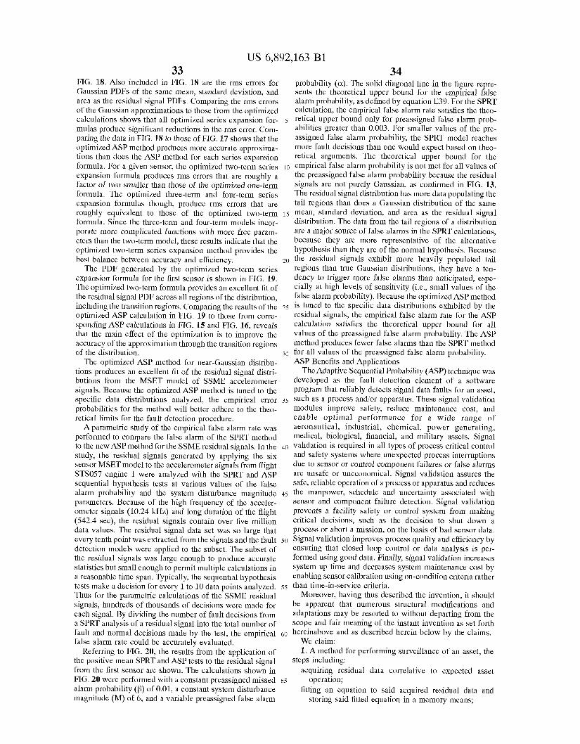
US 6,892,163 B1 35 36

collecting a current set of observed signal data values from the asset;

using said fitted equation in a sequential hypotheses test to determine if said current set of observed signal data

limits for determining unexpected operation of the asset that is indicative of a fault condition.

13. A surveillance system for monitoring an asset, said system comprising in combination:

indicates unexpected operation of the asset that is 5 indicative of a fault condition;

for providing asset surveillance. outputting a signal correlative to a detected fault condition

2. The method of claim 1 wherein the step of acquiring residual data correlative to expected asset operation includes i o acquiring training data values correlative to expected asset operation and obtaining deviations between said training data values and values obtained by using a parameter estimation model wherein said parameter estimation model

3. The method of claim 2 wherein the step of fitting an equation to said acquired residual data and storing said fitted equation in a memory means includes the step of fitting a general probability density function (PDF) to said acquired residual data such that said general PDF is a function of 20 statistical moments of said residual data.

4. The method of claim 3 wherein the step of fitting said general PDF includes the step of fitting a function of a first statistical moment of said residual data, a function of a second statistical moment of said residual data. and a zs

values are a function of said training data values. 15

a data acquisition means for acquiring a current set of signals engendered from said asset correlative to asset status;

a digitizing means for digitizing said current set of signals for defining a current set of digitized signals;

a parameter estimation means for producing a set of estimated signal values as a function of said current set of digitized signals;

a fault detection means for detecting the presence of a fault as a function of said set of estimated signal values and said current set of digitized signals;

said fault detection means including a stored fault detection model comprised of an empirically derived probability density function utilized in a sequential probability test of at least one result of a mathematical operation between said set of estimated signal values and said current set of digitized signals;

a communication means for communicating detected faults to a remote location for providing asset surveillance.

14. The svstem of claim 13 wherein said aarameter function of at least one higher order statistical moment of estimation means for producing said set of estimated signal said residual data. values is of a type individually selected from a group

5. The method of claim 4 wherein said function of a first comprised of a multivariate state estimation technique statistical moment of said residual data is a sample mean. method, a neural network method, a mathematical process

6. The method of claim 4 wherein said function of a 30 model method, a autoregressive moving average method, second statistical moment of said residual data is a sample and a Kalman filter method. variance. 15. The system of claim 14 wherein said empirically

7. The method of claim 4 wherein said function of at least derived probability density function utilized in said sequen- one higher order statistical moment of said residual data is tial probability test is obtained by acquiring training data a sample skewness. 35 values correlative to expected asset operation and obtaining

8. The method of claim 4 wherein said function of at least residual data by computing differences between said training one higher order statistical moment of said residual data is data values and values obtained by using said parameter a sample kurtosis. estimation model on said training data values and fitting a

9. The method of claim 4 wherein said function of at least general probability density function (PDF) to said residual one higher order statistical moment of said residual data is 40 data. a fifth or higher order statistical moment. 16. The system of claim 15 wherein said fitted general

10. The method of claim 3 wherein the step of fitting an PDF is a function of statistical moments of said residual equation to said acquired residual data and storing said fitted data. equation in a memory means includes the step of fitting a 17. The system of claim 16 wherein said general PDF is general probability density function (PDF) to said acquired 45 a function of a first statistical moment of said residual data, residual data by fitting a standard Gaussian PDF to said of a second statistical moment of said residual data, and at acquired residual data and by then adding successive higher least one higher order statistical moment of said residual order terms to said standard Gaussian PDF until an adequate data. agreement between the so derived general PDF and the 18. The system of claim 17 wherein said first statistical actual distribution of said acquired residual data is achieved. SO moment of said residual data is a sample mean.

11. The method of claim 3 wherein the step of using said 19. The system of claim 17 wherein said second statistical fitted equation in a sequential hypotheses test to determine moment of said residual data is a sample variance. if said current set of observed signal data indicates unex- 20. The system of claim 17 wherein said at least one pected operation of the asset that is indicative of a fault higher order statistical moment of said residual data is a condition further includes the step of performing at least one ss sample skewness. of a group of four sequential hypothesis tests comprised of 21. The system of claim 17 wherein said at least one a positive mean test, a negative mean test, a nominal higher order statistical moment of said residual data is a variance test, and a inverse variance test all as a function of sample kurtosis. said general probability density (PDF) function. 22. The system of claim 17 wherein said at least one

12. The method of claim 11 wherein the step of perform- 60 higher order statistical moment of said residual data is a fifth ing at least one of a group of four sequential hypothesis tests or higher statistical moment. comprised of a positive mean test, a negative mean test, a 23. The system of claim 15 wherein said general prob- nominal variance test, and a inverse variance test all as a ability density function (PDF) of said acquired residual data function of said general probability density function (PDF) is comprised of a standard Gaussian PDF and at least one includes the step of processing said at least one of a group 65 higher order term to said standard Gaussian PDF. of four sequential hypothesis tests and comparing an out- 24. A method for training a plurality of process models come of each processed test to upper and lower threshold wherein each process model represents a set of parameter

US 6,892,163 B1 37 38

estimation models and a set of fault detection models of an asset to be monitored by a surveillance system, the steps including:

acquiring at least one set of signal values associated with a current status of said asset;

forming a training data set comprised of at least one said set of signal values;

providing a memory means for storing and retrieving said training data set;

processing said training data set comprised of at least one said set of signal values associated with said current status of said asset for training at least one parameter estimation model;

at least one said parameter estimation model for processing said training data set;

empirically fitting a general probability density function to at least one said set of signals values in said training data set as a function of at least one said estimated set 20 training data set, of process parameters and said training data Set for obtaining at least one empirically derived fault detection model; and

parameter estimation model and at least one said empirically derived fault detection model for subsequent use in surveillance of said asset.

outputting a signal correlative to each detected fault

26. The method of claim 25 ether including a step of forming said stored model.

27. The method of claim 26 wherein the step of forming said stored model includes a step of preparing said stored model using historical operating data from the asset.

28. The method of claim 27 wherein the step of preparing said stored model using historical operating data from the asset further includes a step of creating a training data set having discrete observations correlative to the expected normal operation of the asset wherein each single observation is comprised of a vector of data values from a digitized

estimating at least one set of process parameters by using 15 set of signals correlative to each signal parameter to be included in said stored model.

29. The method of claim 28 wherein said step of forming said stored model includes a step of creating a parameter estimation model by training said stored model using said

30, The method of claim 25 wherein said step of numerically fitting a probability density function to a distribution correlative to normal operation of the asset includes a step

storing within said memory means said at least one said 25 of preparing said fitted probability density function using historical operating data from the asset,

31, ne method of claim 30 wherein the step of preparing said fitted probability density function using historical oper-

30 a training residual data set having discrete residual data

asset wherein each residual data value is comprised of a

and a estimated signal value produced by said stored model

32. The method of claim 31 wherein said step of forming said fitted probability density function includes a step of numerically determining an equation correlative to said training residual data set having discrete residual data values

condition for providing asset surveillance.

25. A method for performing Of an asset, the sting data from the asset further includes a step of creating steps including:

numerically fitting a Probability density function to a

acquiring a current set of observed signal data values from

values correlative to the expected normal operation of the

deviation between a historical operating data signal value distribution correlative to normal operation of the asset;

the asset; calculating a current set of estimated signal data values 35 for said asset.

from a stored model for said asset; transforming said calculated current set of estimated

signal data values with said current set of observed signal data values for defining residual data values;

statistical hypothesis test performed on said residual utilizing said fitted probability density function in a 40 correlative to the expected normal operation of the asset.

data values for detecting a fault condition; and * * * * *

Documents

United States Patent US 6,892,163 B1 - NASA12) United States Patent Herzog et al. (io) Patent No.: (45) Date of Patent: US 6,892,163 B1 May 10,2005 (54 ... Wegerich, S., et al, Challenges