United States Mergers & Acquisitions Market Dynamics: What drives deal flow in each industry? Prepared for the Mathematical Methods in the Social Sciences (MMSS) Program at Northwestern University, 2012

Marco Corrao Northwestern University

Evanston, Illinois

Acknowledgements Though challenging, writing this senior thesis has proven to be a highly satisfying and rewarding experience. The process allowed me to combine the knowledge and expertise I have acquired at Northwestern University with concepts I have become familiar with through internships, while motivating me to greatly expand my understanding. I am grateful to Professor Dimitris Papanikolaou, who devoted much time verifying and challenging my ideas, and always encouraged me to approach the subject from new angles. I am also grateful to Professor Robert J. Gordon, who gave me the opportunity to assist in his research, allowing me to develop my ability to form empirical arguments and provide sound evidence to hypotheses.

The vast library of mergers and acquisitions research has a long history

with no singular focus. Much research has been devoted to the wave-like

behavior and drivers of mergers and acquisitions volume at the aggregate level,

where many links have been established. The existence of merger waves is well

established through the use of autoregressive processes, periodic curve fitting

and parameter switching models. However, the causes of merger waves are not

well agreed upon. Some authors have provided evidence that merger waves are

resultant of clustering M&A activity surges in a small number of industries, and

that clustering occurs only in the presence of sufficient capital liquidity at the

aggregate level, while others have provided contradicting evidence to that

suggestion.

Aggregate M&A activity in the United States has been linked to the capital

markets, cyclic macroeconomic variables, deregulation and business

expectations. The derived relationships between M&A activity and these

variables appears to be highly dependent on the type of data the author uses, as

well as the way the data is transformed for econometric purposes, evidenced by

inconsistency in the findings among similar research papers. Various authors

define M&A activity as the ratio of acquisitions to the total number of firms, while

others logarithmically transform M&A volume and take first differences. For

some variables, such as the cost of capital, evidence is provided in various

papers that could be used to argue just about any hypothesis about the influence

of the cost of capital. Some research finds positive relationships, yet other

research provides evidence of negative relationships or no significance at all.

The drivers of industry specific M&A activity in the United States have not

been researched as comprehensively as aggregate M&A activity, nor have the

drivers of M&A activity in those industries been methodically compared. Further,

industry specific M&A activity research has seldom been focused on from a

forecasting perspective. This paper separates M&A activity in the United States

into industry groups and explores the drivers in each from a forecasting

perspective, asking the following question: What drives mergers and acquisitions

activity in each industry in the United States, and how do those drivers vary

across industries?

To address the above question, this paper will first survey the universe of

relevant literature, which includes research on the existence and causes of

merger waves, as well as the drivers of M&A activity. Afterwards, we will

introduce the data utilized in this study and present the analysis of the data,

which first derives econometric relationships between M&A activity in each

industry and various drivers, and then compares the drivers across industries.

This paper will end with the key findings and conclusions, as well as suggestions

for further research.

LITERATURE REVIEW

An extensive amount of research pertaining to the relationships between

the mergers and acquisitions market and the United States economy has been

focused around the existence of merger waves, the causes of merger waves,

and the drivers of mergers and acquisitions volume. Evidence of the existence of

merger waves in United States has been uncovered in historical data through

autoregressive processes (Stughart & Tollison, 1984; Golbe & White, 1988;

Barkoulas et al., 2001), fitting a sine curve to historical merger data (Golbe &

White, 1993), and parameter switching models such as the Markov regime-

switching model (Town, 1992; Resende, 2005; Gärtner & Halbheer, 2009).

Merger waves have been hypothesized and shown to be derived from clustering

of surges within a small number of industries (Mitchell & Mulherin, 1996; Boone &

Mulherin, 2000; Andrade et al., 2001; Harford, 2005), while recent evidence

contradicting those theories has also been provided (Gärtner & Halbheer, 2009).

Mergers and acquisitions volume has long been tied to the capital markets and

business cycle related macroeconomic variables (Nelson, 1959; Beckenstein,

1979; Melicher et al., 1983; Clarke & Ioannidis, 1996), as well as technological

innovation (Gort, 1969), Tobin's "q" (Golbe & White, 1988), and more recently

tied to business expectations (Carapeto et al., 2010) .

Using autoregressive processes, empirical evidence was first produced

against the existence of merger waves, but this theory was quickly challenged.

Using United States merger data from 1895 to 1979, Stughart and Tollison were

unable to provide evidence that merger activity is not generated simply by a

random walk or white-noise process (Stughart & Tollison, 1984). However, they

did not actually test a wave hypothesis explicitly; they simply could not reject the

null hypothesis that merger activity is governed by a first order autoregressive

process, which provoked future researchers to challenge their findings. Golbe

and White later uncovered a strong autoregressive dependence in quarterly

mergers and acquisitions data, showing empirically that both first and second

order autoregressive terms have very strong explaining power, providing

evidence against the white-noise theory (Golbe & White, 1988) .

Through successfully fitting a sinusoidal curve to annual data on mergers

and acquisitions from 1919 through 1979, Golbe and White provided evidence of

the existence of merger waves in the United States. After identifying positive

serial correlation in the data, first differences were taken in combination with

ordinary least squares estimation to find positive and statistically significant wave

amplitude and frequency coefficients in the sinusoidal model. Through this

estimation, Golbe and White hypothesized a period of 40 years for the merger

waves. The peaks and troughs in the fitted values were qualitatively determined

to line up roughly with the peaks and troughs in the actual merger data.

Significant explanatory power was provided with their basic sinusoidal model, so

they neglected to explore more complex wave forms, leaving that possibility for

future research. (Golbe & White, 1993)

Contrary to the findings of Stughart and Tollison and partially in support of

merger wave evidence provided by Golbe and White, long-term memory and

dependence in merger data were uncovered using higher order autoregressive

processes as well as autoregressive fractionally integrated moving average

processes (ARFIMA) (Barkoulas et al., 2001). These ARFIMA processes can

give rise to waves or stretches of high and low values without regularity or well

defined periodicity, supporting the existence of merger waves without requiring

the well defined periodicity of a sine wave, which Golbe and White hypothesized.

(Barkoulas et al., 2001)

Using a nonlinear, two-state, Markov regime-switching model, Town

captured merger wave behavior and fit United States mergers data better than

previously used linear ARIMA models using five distinct data sets used in

previous merger research. Town claimed that linear models fail to adequately

capture the behavior of the merger data and that his nonlinear, Markov regime-

switching model is more appropriate. He concluded that mergers and

acquisitions alternate between a high mean and variance state and a low mean

and variance state, consistent with wave characterization. He also used his

model to identify specific merger waves in the historical data and identified nine

distinct merger waves between 1898 and 1986. (Town, 1992)

Similarly to Town, others have more recently employed a two-state,

Markov regime-switching model to fit merger data in both the United States and

United Kingdom. Resende was able confirm that even for the U.K. mergers data,

the model captures behavior well and that persistence and long-term memory

appear to be important features (Resende, 2005). Gärtner and Halbheer used

quarterly data from 1973 to 2003 to identify merger waves in the U.S. and U.K.,

but were only able to identify the beginning of a merger wave in the U.S. in 1995,

and not the 1980s merger wave that Town uncovered. They conjecture that the

reason a 1980s merger wave was not uncovered is because it was dwarfed in

the data by the 1990s wave and that the 1980s activity actually looks more

normal in comparison. Gärtner and Halbheer also hypothesized that previous

econometric misidentifications of the 1980s merger wave could have been due to

the use of less refined inference methods (Gärtner & Halbheer, 2009).

Since the existence of merger waves has been well established,

researchers have begun focusing more on the causes of merger waves. One of

the prominent theories has been that aggregate merger waves are derived from

the clustering of mergers and acquisitions activity surges at the industry level

(Mitchell & Mulherin, 1996; Boone & Mulherin, 2000; Andrade et al., 2001;

Harford, 2005). These M&A activity surges at the industry level are further

hypothesized to be a direct result of firms responding rationally to industry

shocks in the presence of sufficient capital liquidity (Harford, 2005).

Mitchell and Mulherin took a close look at the causes of the merger wave

of the 1980s by separating mergers activity into 51 distinct industries and using

basic regression analysis, including dummy variables, to conclude that industry

specific shocks such as deregulation, financing innovations, and changes in input

costs cause merger waves at the industry level (Mitchell & Mulherin, 1996). Their

analysis, unfortunately, restricts merger waves to be two years in duration for

each industry without much explanation.

A few years later, similarly, Mulherin and Boone found significant industry

clustering during the U.S. merger wave of the 1990s, placing a strong emphasis

on the importance of deregulation in industry level mergers and acquisitions

activity surging. They also provided empirical evidence discounting the notion

that M&A activity in the 1990s was restricted to growth starved industries. (Boone

& Mulherin, 2000)

Andrade, Mitchell, and Stafford provided additional evidence in favor of

the notion of industry shocks and industry level clustering and took it a step

further, claiming that deregulation became a dominant factor in mergers and

acquisitions activity in the 1990s, accounting for nearly half of the activity since

then. They arrived at this notion by defining a ten-year "deregulation window"

around each deregulation event, and find that during the 1980s, roughly 10-15%

of total merger activity was represented by industries in a deregulation window,

and that in the 1990s, this percentage rose to nearly half of all annual deal

volume. Little motivation behind the reason that the deregulation window should

be ten years in length is provided, however, and the evidence is not compelling

for a well defined causal link between the lengthy deregulation window and

mergers volume. Interestingly, by ranking merger activity in each industry over

time and correlating across decades, they found no correlation and concluded

that industries that undergo mergers and acquisitions activity surges in one

decade are no more likely to do so in other decades. Strengthening their point,

they showed that the top five industries by merger value in the 1980s differ

completely from the top five industries in the 1990s. (Andrade et al., 2001)

A more compelling link has been made between aggregate merger waves

and industry level merger activity surges by Harford. Harford claimed that

industry shocks cause merger activity surges at the industry level only in the

presence of sufficient capital liquidity and that this macro-level capital liquidity

causes industry merger waves to cluster in time, even if the industry shocks do

not. By employing logit models to predict the start of industry merger waves,

Harford found that deregulatory, industry-specific shocks, and capital liquidity

have the strongest predictive power. He also discovered that behavioral market

oriented variables, such as industry return and standard deviation of returns, only

add marginal predictive power. In the aggregate, Harford used the spread

between the average interest rate on commercial and industrial loans and the

federal funds rate as a proxy for capital liquidity, and industry weighted analogs

to his variables at the industry level in his logit model. From his results, Harford

noted that a high rate spread reduces aggregate merger activity, behavioral

market oriented variables are insignificant, and, shockingly, that deregulation is

insignificant in the aggregate model, despite its tremendous importance in the

industry level data. He concluded that aggregate merger waves are not

propagated by managers attempting to time the market, and that his findings

support his hypothesis regarding merger waves and capital liquidity. (Harford,

2005)

Recent empirical findings by Gärtner and Halbheer contradicted the

prominent notion that the clustering of mergers and acquisitions activity industry

level surges are the cause of waves in aggregate merger activity. Using a two-

state, Markov regime-switching model, they identified the 1995 merger wave and

then dissected that specific wave at the industry level. By plotting the U.S.

industry level merger activity between 1990 through 2003 for the top eleven

industries, Gärtner and Halbheer determined qualitatively that industries were not

simultaneously hit with the 1995 merger wave, and that the aggregate wave was

not the result of a few industry level bursts. After having removed the eleven

most active industries in terms of annual merger activity, accounting for 52-66%

of the aggregate, the remaining merger activity still resembled a strong wave.

(Gärtner & Halbheer, 2009)

Aside from the drivers of mergers and acquisitions activity in the context of

merger waves, a tremendous amount of research has been devoted to linking

M&A volume to the capital markets, business cycle related macroeconomic

variables, and business expectations. Nelson noticed that early mergers and

acquisitions surges or waves occurred during a cyclically rising stock market,

prompting him to investigate the relationships between aggregate volume and

various capital market and macroeconomic conditions. Using de-trended data

from 1895 to 1954, Nelson conducted correlation analysis between mergers and

acquisitions volume and an industrial stock index's level and trading volume, as

well as the index of industrial production. Nelson claimed that aggregate merger

activity was more responsive to changes in the capital markets than changes in

the level of production, but that it is not clear if the importance of each is causal.

Nelson also analyzed the peaks and troughs in the aggregate mergers

and acquisitions activity with those in the industrial stock index level and volume,

industrial production level, and business cycle as defined by the National Bureau

of Economic Research. During expansions, Nelson noticed that typically there is

a peak in stock trading volume first, followed by peaks in merger activity, stock

prices, business incorporations, the business cycle, and lastly, industrial

production. He noticed during contractions that there normally is a trough in stock

prices first, followed by troughs in stock trading, business incorporations, merger

activity, industrial production, and the business cycle. Although Nelson's research

did not involve typical empirical methods by modern standards or provide solid

evidence of any causal relationships, his findings catalyzed future research on

the subject of mergers and acquisition activity dynamics. (Nelson, 1959)

One decade later, Gort attempted to unravel the drivers of the merger

rate, the ratio of the number of acquisitions to the number of firms, and claimed

that the most common economic shocks resulting in mergers activity were rapid

changes in technology and movements in securities prices, because they caused

a dispersion in valuations. Using data on mergers and acquisitions from 1951 to

1959 classified by industry, Gort performed various econometric analyses, but

ultimately restricted the study to the manufacturing related industries. Two

proxies were used for technological change: the technical personnel ratio,

measured as the number of engineers, chemists and surveyors per 10,000

employees, and the change in labor productivity over time. The concentration

ratio, the proportion of industry output contributed by the four largest producers,

was taken as a measure of barriers to entry and large firm dominance.

Empirically, Gort's econometric models showed that the technical personnel ratio,

productivity change, and the concentration ratio were each strongly correlated

with merger rates. Lack of stock price indexes that matched his industry level

data prevented Gort from properly introducing a stock price variable into the

analysis, but he was able to analyze the stock prices of buyers and targets in

specific mergers and determined there was no pronounced tendency for buyers

to have higher price to earnings ratios than sellers. (Gort, 1969)

In a study of manufacturing and mining merger activity from 1958 to 1975,

Beckenstein introduced interest rates on prime commercial paper into his

econometric models to capture the effects of the cost of capital on merger

activity, along with S&P 500 returns and GNP levels and growth. Through

running permutations of his variables, Beckenstein found that the level of the

S&P 500 index and the cost of capital proxy variables were significant in the most

econometrically sound models, but that the coefficients do not suggest any

important role, numerically. Surprisingly, the influence of the cost of capital proxy

variables were found to be positive and significant, whereas one might expect the

coefficients to be negative since they are directly related to the cost of the

merger. Notably, Beckenstein's GNP variable lacked success; it was rarely

significant and sometimes had negative coefficients, contrary to intuition.

Beckenstein also attempted to implement some log-log models but had difficulty

with interpretation and could not achieve a better fit through using them.

(Beckenstein, 1979)

In a study between aggregate merger activity, industrial activity, business

failures, stock prices and interest rate levels, Melicher, Ledolter, and D'Antonio

first used cross correlation techniques between variables to determine proper lag

and lead structures for variables and then constructed econometric models. They

discovered that mergers and acquisitions activity lags stock market movements

and bond yields but leads changes in production, so they restricted their model to

include past and present stock prices and bond yields. Using quarterly data

covering the 1947 to 1977 time period, their empirical results indicated a weak

relationship between merger activity and changes in industrial production, but

they had some success with the capital markets variables. They concluded that

changes in stock prices and bond yields can be used to forecast future changes

in merger activity and that higher stock prices and lower interest rates seem to

lead to increased merger activity, partially contradictory to Beckenstein's findings

related to the effects of the cost of capital. (Melicher et al., 1983)

In addition to readdressing the cost of capital hypothesis, Golbe and White

introduced relative price changes, changes in tax regimes, and Tobin's "q" in

their analysis of mergers and acquisition patterns. As a proxy for the cost of

capital, they constructed a variable that is a the rate on a Aaa-rated corporate

bond less the inflation rate for use in their models, but they were unable to

achieve statistical significance using regular OLS estimation. By computing the

variance of price changes of the major components of the BLS wholesale price

index and the producer price index and aggregating into quarterly values, they

created a proxy for changes in economic circumstances, but the variable was

insignificant in the model. Tax regime dummy variables were included to account

for the 1954, 1963, and 1981 tax regime changes, but they did not add explaining

power to the model. Golbe and White also implemented Tobin's q, the ratio of

market value to replacement cost, with the expectation that lower q implies a

greater bargain, leading to more merger activity. The coefficient on Tobin's q in

their regressions was estimated to be positive and significant, which contradicts

their hypothesis. Golbe and White found stronger results by running regressions

on logarithmically transformed data but still were generally unsuccessful in

uncovering the dynamics between fundamental economic factors and mergers

and acquisitions activity. (Golbe & White, 1988)

Focusing on the reliability of stock market conditions as predictors of

merger activity, Clarke and Ioannidis tested quarterly data on merger activity in

the U.K. from 1969 to 1994 for Granger causality. They ran econometric models

and Granger causality tests in both directions, testing whether stock market

returns Granger cause mergers and acquisitions activity and also testing whether

mergers and acquisitions activity Granger causes stock market returns. The

hypothesis of "non-causality" from stock market returns to mergers and

acquisitions activity was rejected at the 5% level, and they were unable to reject

the complementary hypothesis ("non-causality" from mergers activity to stock

market returns). From these results, they concluded that stock market returns

Granger cause mergers and acquisitions activity in the U.K.. (Clarke & Ioannidis,

1996)

A much more recent study presented by Carapeto, Dallocchio, Faelten,

Lanzolla, and Moeller investigates whether business expectations are useful in

predicting mergers and acquisitions activity. The authors identified three

constituencies of business expectations, including analyst expectations,

management expectations, and media expectations. Analyst expectations were

measured as the number of buy or sell recommendations in a quarter, the proxy

for management expectations was the CEO confidence index, and media

expectations were calculated as the number of occurrences of M&A related

articles reported by FACTIVA. Using time series and panel data analysis on the

first differences of logarithmically transformed U.S. and U.K. mergers data for the

1984 to 2009 time period, they claimed that changes in analyst expectations and

management expectations predict and drive mergers and acquisitions activity,

but the predictive power is only significant when lagged one quarter. In the U.K.

data, their tests unveiled a positive relationship between the number of mergers

and acquisitions related articles covered by the media and actual M&A activity.

One inherent flaw in their work, however, is that their analyst expectation variable

contains unwanted growth because analyst coverage and the number of equity

analysts have both been increasing dramatically over time. This results in large

increases in the number of buy ratings released over time, but does not

necessarily reflect a more optimistic outlook from analysts. A simple scaling by

the total number of equity ratings released would have alleviated this issue, but it

does not appear that they employed any sort of scaling. The authors

acknowledge that it would be interesting for future research to investigate these

relationships at the industry level, rather than at the aggregate level. (Carapeto et

al., 2010)

In a study of the characteristics leveraged buy-out targets in the United

States, it was discovered that more buy-outs occur when risk-free rates are high

and the risk premium is low. Using probit models to find the likelihood of a firm

going private, the study shows empirically that firms are less likely to LBO if they

have high exposure to systematic shocks and higher idiosyncratic risk, which

translates directly to high market beta, residual variance, or cash flow volatility.

Although leveraged buy-outs have important differences from a typical M&A

transaction, extending these ideas into the realm of M&A activity is a small leap.

(Haddad et al., 2011)

The vast amount of research related to the behavior of mergers and

acquisitions activity and its drivers spans widely; from the existence and causes

of merger waves, to macroeconomic and capital market dynamics, as well as the

predictive power of business expectations. Much of this research revolves

around aggregate mergers and acquisitions volume or a specific set of drivers.

Few researchers have broken the issue down to the industry level to unveil

distinctions in the dynamics and drivers across industries from a forecasting

perspective, which will be the focus of this paper.

DESCRIPTION OF DATA

Much of the data used in this paper is easily accessible online, with a few

key data series sourced from Bloomberg and Capital IQ databases.

M&A Volume

Mergers and acquisitions volume data was pulled from Capital IQ

database for 1976 through 2011. I restricted inclusion to target companies in the

United States with transaction value greater than $25mm, and generated industry

specific M&A volume data by aggregating individual deals in each industry for

every quarter in the time series. Transaction values were recorded at historical,

nominal values in US dollars. Overall, M&A volume data for the United States

does not appear to be complete in the early years of the data set, but this issue is

transient.

Gross Domestic Product

GDP is seasonally adjusted data from the Bureau of Economic Analysis

National Income and Product Accounts Table 1.15.

Industrial Production

The Index of Industrial Production data was pulled from series G.17 on the

Federal Reserve website. IIP is seasonally adjusted and indexed to 2007 = 100.

S&P Stock Market Indices

Standard & Poor stock market indices were pulled for the aggregate US

stock market, as well as for each industry. For the aggregate US stock market,

the S&P 500 Index was pulled from Yahoo! Finance historical values, and

aggregated into quarterly data via closing prices on the final day of each quarter.

The industry specific S&P stock market indices were collected from Bloomberg.

Stock Market Uncertainty

The 90-day historical volatility in the S&P stock market indices was used

as a proxy for uncertainty in the market and was pulled from Bloomberg for each

industry, as well as for the S&P 500. A glaring issue with using historical volatility

as a proxy for market uncertainty is that it is not forward looking, which is more

appropriate for use in forecasting models. Preferably, the proxy variable for

uncertainty in the stock market should be the implied volatility, which is backed

out of the Black-Scholes model using historical options prices. However,

historical option prices on the S&P industry specific indices were not available

through any of my resources, so historical volatility will have to suffice.

Industry Risk Premium

I defined the risk premium for each industry as the market beta of the S&P

industry specific index using two years of historical weekly returns from

Bloomberg.

Analyst Expectations

I derived the proxy for analyst expectations from equity analyst ratings via

Bloomberg. For each industry, the average buy/sell rating on a scale from 1 to 5

for every equity for a given quarter was pulled, which were then averaged to

achieve a quarterly equity analyst rating series for each industry. This data is

only available as far back as the mid 1990s, where the data begins very sparsely

and gradually becomes more complete. Interestingly, the average equity analyst

rating never dips below neutral for any quarter, implying that equity analysts tend

to be optimistic on average, and that they don't necessarily predict economic

downturns. This also implies an analyst coverage bias towards strong performing

equities. High levels of the average equity analyst rating for an industry can be

interpreted as optimistic analyst expectations of the future, and quarterly

increases in the average rating can be interpreted as increasingly optimistic

analyst expectations.

Debt Yields

The daily yields on Aaa-rated and Baa-rated corporate debt from Moody's

were attained from the Board of Governors of the Federal Reserve System

website, as well as the yield on 10-year treasuries from the US Department of

Treasure Resource Center. For each series, the daily yields were averaged to

form quarterly debt yield data.

ANALYSIS

To properly determine and assess the drivers of M&A volume and how

they vary across general industry groups, I have constructed econometric models

at the aggregate level and for each industry to estimate the effects of plausible

macroeconomic, capital markets and expectation oriented variables. I will briefly

discuss the reasoning behind the inclusion of each variable, provide a prediction

of its effect on M&A activity, and then analyze the output of each model. Lastly, I

will compare the results across industries.

Variable Description

The dependent variable in each model is a time series of the level of M&A

activity in industry i, which is defined as follows:

(1) M&Ai,t = M&A Volumei,t / GDPt

This defines M&A activity as the volume of M&A in each industry scaled

by the level of GDP, both of which are in nominal terms for consistency. Through

scaling by GDP, we partially control for the effects of the business cycle on M&A

activity, as well as the time trend, and our definition of M&A activity is relative to

GDP. Previous research has uncovered memory in M&A activity through

modeling M&A activity with autoregressive processes (Barkoulas et al. 2001). For

this reason, the first lag of the dependent variable is included in each model, as

well as a second lag in models where it has shown significance.

Figure 1

Aggregate M&A ActivityM&A aggregate

0

10

20

30

40

50

60

70

80

90

1995

1996

1997

1998

1999

2000

2001

2002

2003

2004

2005

2006

2007

2008

2009

2010

2011

Year

In Figure 1 above, it is clear that M&A activity tends to spike upwards and then

quickly downwards, rather than plateau for some period of time. Because of this,

I expect the coefficients on M&Ai,t-1 to be negative, promoting unsustainability in

high levels of M&A activity.

Past research has established links between industrial production M&A

activity in varying degrees of strength and importance, but the majority of the

relationships were investigated using aggregate M&A volume (Nelson, 1959;

Melicher et al., 1983). I posit that, when broken down at the industry level,

industrial production will show varying significance and importance across

models, due to industrial production having less relevance in some industries

than others. To capture the effects of industrial production on M&A activity, the

following variable is defined:

(2) Industrial Prodt = IIPt / GDPt

where IIPt is the index of industrial production. The first lag of Industrial Prod will

be included in each model. Since high industrial production is an indicator of a

healthier economy, I suggest there is a positive relationship between M&A

activity and industrial production in general. However, there have been

substantiated claims that industrial production peaks after M&A activity peaks

(Nelson, 1959), so high industrial production could also mean a large amount of

mergers just occurred. For this reason, a negative effect could arise in some

industry models as well. Below, Figure 2 depicts the relationship between

aggregate M&A activity and industrial production over the sample period.

Figure 2

Aggregate M&A Activity vs. Industrial ProductionRelative to GDP

0

10

20

30

40

50

60

70

80

90

1995

1996

1997

1998

1999

2000

2001

2002

2003

2004

2005

2006

2007

2008

2009

2010

2011

0.0055

0.006

0.0065

0.007

0.0075

0.008

0.0085

0.009

0.0095

0.01

M&A (L) IP (R)

An ample amount of research has long linked stock prices to M&A activity,

the general notion being that M&A activity lags stock market movements (Nelson,

1959; Melicher et al., 1983), and Granger causality was also established (Clark &

Ioannidis, 1996). The variable used to capture the effects of the stock market

with respect to each industry i is defined as follows:

(3) Stocksi,t = S&P Indexi,t / GDPt

where S&P Indexi is the S&P Industry i market capitalization weighted index

level. The first lag of this variable is included in each model, and for the

aggregate model the S&P 500 Index is used. Consistent with previous research, I

predict the coefficient on Stocksi,t-1 will be positive, since M&A activity and the

stock market have typically fluctuated together, as seen below in Figure 3.

Figure 3

Aggregate M&A Activity vs. S&P 500 PerformanceRelative to GDP

0

10

20

30

40

50

60

70

80

90

1995

1996

1997

1998

1999

2000

2001

2002

2003

2004

2005

2006

2007

2008

2009

2010

2011

0.05

0.07

0.09

0.11

0.13

0.15

0.17

M&A (L) S&P 500 (R)

In order to incorporate the effects of stock market uncertainty in the model,

I included the 90-day historical volatility of industry i's S&P index returns, named

Uncertaintyi,t. The first lag, Uncertaintyi,t-1, is included in each model. Uncertainty

in the market typically makes ordinary M&A transactions riskier, because the

target valuation and pro-forma analysis of the transaction relies heavily on future

projections. As uncertainty in the market increases, confidence in those

projections, and, ultimately, the valuation itself, decrease. Because of this, I

expect the coefficient on Uncertaintyi,t-1 to be negative for all industries,

suggesting that uncertainty during one quarter will result in lower M&A activity in

the next. Figure 4 below plots Telecom M&A activity against S&P Telecom Index

volatility, which clearly illustrates the absence of Telecom M&A activity during

periods of high uncertainty.

Figure 4

Telecom M&A Activity vs. S&P Telecom Index UncertaintyRelative to GDP

0

2

4

6

8

10

12

14

16

1995

1996

1997

1998

1999

2000

2001

2002

2003

2004

2005

2006

2007

2008

2009

2010

2011

0

10

20

30

40

50

60

70

Telecom M&A (L) Volatility (R)

Recently, a link has been established between leveraged buy-out

transactions and changes in risk premiums. It was discovered that firms with

higher exposure to systematic shocks, or higher market beta, are less likely to be

bought out (Haddad et al., 2011). Extending this idea into the realm of M&A

transactions in general requires a slight caveat, because LBO transactions are by

definition financed with a high level of debt. For this reason, the acquirers prefer

the cash flows and performance of the target to be more predictable and less

dependent on systematic shocks so that the interest payments on the high level

of debt can be made without any default. Since M&A encompasses transactions

that are not always funded with debt, the effect of changing risk premiums is

likely diluted relative to the effect it has on LBO transaction activity.

In order to incorporate the effects of varying levels of risk premium, I have

included Betai,t-1, the first lag of the beta of industry i's S&P Index with respect to

the market, in each industry's model. For the reasons highlighted above, I

anticipate that the coefficient on Betai,t-1 will be negative. I also will experiment

with the first difference of Betai,t-1 in the models to incorporate changes in risk

premium, which I also expect to have a negative coefficient with similar

reasoning. Below, Figure 5 depicts the inverse relationship between Utilities

M&A activity and the S&P Utilities market beta.

Figure 5

Utilities M&A Activity vs. S&P Utilities BetaRelative to GDP

-2

-1

0

1

2

3

4

5

1995

1996

1997

1998

1999

2000

2001

2002

2003

2004

2005

2006

2007

2008

2009

2010

2011

0.2

0.3

0.4

0.5

0.6

0.7

0.8

0.9

Utilities M&A (L) Utilities Beta (R)

Changes in analyst expectations were also recently tied to M&A activity

through the use of equity analyst buy and sell ratings (Carapeto et al., 2010).

However, the authors define changes in analyst expectation as the quarterly

change in the number of buy ratings released in a quarter for US equities. This is

inherently flawed because analyst coverage has been increasing greatly over

time, as well as the number of analysts, which creates a major unwanted

increase in their proxy for analyst expectations from quarter to quarter.

In order to alleviate this issue, I created a different proxy for analyst

expectation that averages all consensus analyst equity ratings on all equities in

an industry, named Analysti,t, which varies from 1 (strong sell) to 5 (strong buy)

over time. In effect, Analysti,t represents the average equity analyst rating for

industry i at time t. The first lag of this proxy for analyst expectation will be

included in each industry model. Consistent with previous findings, I expect the

coefficient on Analysti,t-1 to be positive, since more optimistic expectations of the

market should provoke increased M&A activity. Similarly to the risk premium

variable, I will also experiment with the first difference of Analysti,t-1 in order to

reveal the effects of changes in analyst expectation, which I also expect to have

a positive coefficient for the same reasons. Figure 6 portrays this positive

relationship between Energy M&A activity and equity analyst expectations of the

Energy industry.

Figure 6

Energy M&A Activity vs. Analyst ExpectationsRelative to GDP

0

2

4

6

8

10

12

1995

1996

1997

1998

1999

2000

2001

2002

2003

2004

2005

2006

2007

2008

2009

2010

2011

3.0

3.2

3.4

3.6

3.8

4.0

4.2

4.4

4.6

4.8

Energy M&A (L) Analyst Ex. (R)

Debt capital markets are a key factor in M&A transactions due to their

importance in valuation as well as in financing transactions. The relationship

between bond yields and M&A activity has been researched thoroughly in the

past and has been identified as a key factor, but with mixed results. A positive

relationship was uncovered between the cost of capital and M&A activity in some

research (Beckenstein, 1979), others revealed the opposite in later research

(Melicher et al., 1983; Harford, 2005), while yet more research found its role to

be insignificant (Golbe & White, 1988).

In order to incorporate the effects of the cost of capital on M&A activity, I

have introduced several bond yield and credit spread variables into the models

for each industry. AaaBondt-1 is the first lag of the average yield on a Aaa

corporate bond from Moody's, and Treasuryt-1 is the first lag of the yield on the

10-year treasury note. Aaa-Treasuryt-1 and Baa-Treasuryt-1 represent the first lags

of credit spreads for Aaa and Baa corporate bonds from Moody's relative to the

yield on the 10-year treasury note.

Since the cost of M&A transactions scale with the bond yields, I expect

negative coefficients on each of the bond yield variables. Widening credit

spreads signal pessimistic outlooks as well as uncertainty in the corporate

domain, so I expect negative coefficients on the credit spread variables as well,

consistent with the findings of Harford (Harford, 2005). I will also experiment with

the first differences of these variables to see if changes in the cost of capital and

credit spreads have a more pronounced impact on M&A activity than levels. I

expect the coefficients on the first-differenced variables to also be negative with

similar reasoning. Figure 7 and Figure 8 below plot Tech M&A activity against

bond yields and Consumer Discretionary M&A activity against credit spreads,

respectively.

Figure 7

Tech M&A Activity vs. Bond YieldsRelative to GDP

0

2

4

6

8

10

12

14

16

18

20

1995

1996

1997

1998

1999

2000

2001

2002

2003

2004

2005

2006

2007

2008

2009

2010

2011

0.0

1.0

2.0

3.0

4.0

5.0

6.0

7.0

8.0

9.0

Tech M&A (L)

Aaa (R)

Treasury (R)

Figure 8

CD M&A Activity vs. Credit SpreadsRelative to GDP

0

5

10

15

20

25

1995

1996

1997

1998

1999

2000

2001

2002

2003

2004

2005

2006

2007

2008

2009

2010

2011

0.0

1.0

2.0

3.0

4.0

5.0

6.0

CD M&A (L)

Aaa-Treasury (R)

Baa-Treasury (R)

Sample Period

The sample period for the Consumer Discretionary, Energy, Financials,

Healthcare, Materials, Technology and Utilities industries, as well as the

Aggregate model, is 1997:Q2 to 2011:Q4. For the Consumer Staples, Industrials

and Telecommunications industries, the sample period is 1997:Q3 to 2011:Q4.

Aggregate Model

The full model for aggregate M&A activity is as follows:

(4) M&AAggregate,t = β0 + β1M&AAggregate,t-1 + β2Industrial Prodt-1 +

β3StocksAggregate,t-1 + β4UncertaintyAggregate,t-1 + β5AnalystAggregate,t-1 + β6AaaBondt-1

+ β7Treasuryt-1

Aggregate Model

Variable Coefficient Std. Error

M&A Aggregate,t-1 -0.04 (0.27)

Industrial Prod t-1 875.75 (0.33)

Stocks Aggregate,t-1 643.81 *** (4.16)

Uncertainty Aggregate,t-1 0.33 (1.50)

Analyst Aggregate,t-1 -1.65 (0.14)

AaaBond t-1 -11.53 ** (2.18)

Treasury t-1 3.97 (0.91)

Constant 3.98 (0.14)

F Statistic 8.76

Adjusted R2

0.48

N 59

* p <0.1; ** p <0.05; *** p <0.01

In the aggregate model, many of the variables are very close to being

significant at the 10% level, but do not quite make it. As expected,

StocksAggregate,t-1 has a positive and highly significant coefficient, suggesting that

high aggregate stock market values relative to GDP in one quarter predicts high

levels of aggregate M&A volume in the next. Also, the coefficient on Aaa-rated

corporate bond yields is significant and negative, as expected, suggesting that

high, increasing bond yields lead to depressed M&A activity at the aggregate

level. This is likely resultant of the increased costs associated with M&A

transactions as bond yields increase. Note that the credit spread variables were

highly insignificant in the aggregate model and that bond yield levels better

described the data.

Consumer Discretionary Model

The full model for Consumer Discretionary M&A activity is as follows:

(5) M&ACD,t = β0 + β1M&ACD,t-1 + β2Industrial Prodt-1 + β3StocksCD,t-1 +

β4D1(Uncertainty)Aggregate,t-1 + β5D1(Beta)CD,t-1 + β6AnalystCD,t-1 +

β7Aaa-Treasuryt-1 + β8Baa-Treasuryt-1

Consumer Discretionary Model

Variable Coefficient Std. Error

M&A CD,t-1 -0.38 *** (3.02)

Industrial Prod t-1 988.66 (1.28)

Stocks CD,t-1 748.24 *** (4.34)

D 1 (Uncertainty) Aggregate,t-1 -0.13 ** (2.29)

D 1 (Beta) CD,t-1 25.40 * (1.89)

Analyst CD,t-1 -1.47 (0.44)

Aaa-Treasury t-1 -6.18 ** (2.53)

Baa-Treasury t-1 3.53 ** (2.45)

Constant -11.60 (1.43)

F Statistic 7.19

Adjusted R2

0.46

N 59

* p <0.1; ** p <0.05; *** p <0.01

In the Consumer Discretionary M&A activity model, high statistical

significance was revealed in several variables. The coefficient on the lagged

dependent variable is significant and negative as anticipated, suggesting that

high levels of M&A activity are typically not sustained; rather, they are relatively

short lived. The coefficient on StocksCD,t-1 is positive and significant as expected,

signifying a positive relationship between M&A activity in the Consumer

Discretionary industry and the market valuation of publicly held Consumer

Discretionary companies. The aggregate market uncertainty variable has a

negative and significant coefficient, which agrees with the notion that economic

uncertainty is detrimental to M&A activity. Interestingly, this model preferred

aggregate uncertainty to uncertainty specific to the Consumer Discretionary

industry, suggesting that M&A activity in this industry is more influenced by the

health of the economy as a whole, rather than a subset of industry specific

factors. The significant positive coefficient on the D1(Beta)CD,t-1 suggests that

increases in Consumer Discretionary risk premiums with respect to the market in

one quarter should lead to an increase in Consumer Discretionary M&A activity in

the next, contrary to my hypothesis. It's possible that increasing risk premiums in

the Consumer Discretionary industry provokes significant long term investment to

fuel growth and promote diversification, and that some firms utilize M&A as a

strong source of inorganic growth and stability.

The credit spread variables are both significant but are surprisingly

opposing in sign. Historically, the magnitude of the Baa-Treasury spread has

been roughly 1.7x that of the Aaa-Treasury spread on average, while the

estimated beta coefficient on the Aaa-Treasury spread is roughly -1.8x the

coefficient on the Baa-Treasury spread. This suggests that these two credit

spread variables are typically correcting and canceling each other in the

estimation process, but the overall effect is slightly negative. These results are

consistent with the idea that widening credit spreads signals a pessimistic

outlook, while directly increasing the cost of financing M&A transactions,

therefore prefacing decreased M&A activity.

Consumer Staples Model

The full model for Consumer Staples M&A activity is as follows:

(6) M&ACS,t = β0 + β1M&ACS,t-1 + β2Industrial Prodt-1 + β3StocksAggregate,t-1 +

β4D1(Uncertainty)CS,t-1 + β5D1(Beta)CD,t-1 + β6D1(Analyst)CS,t-1 + β7AaaBondt-1 +

β8D1(Treasury)t-1

Consumer Staples Model

Variable Coefficient Std. Error

M&A CS,t-1 0.02 (0.14)

Industrial Prod t-1 -706.62 ** (2.24)

Stocks Aggregate,t-1 48.62 *** (3.66)

D 1 (Uncertainty) CS,t-1 -0.02 (0.66)

D 1 (Beta) CS,t-1 7.48 ** (2.25)

D 1 (Analyst) CS,t-1 1.47 (0.62)

AaaBond t-1 0.31 (0.80)

D 1 (Treasury) t-1 -0.92 * (1.79)

Constant -0.92 * (1.79)

F Statistic 2.56

Adjusted R2

0.18

N 58

* p <0.1; ** p <0.05; *** p <0.01

The Consumer Staples M&A activity model reveals statistical significance

in the industrial production variable, with a negative coefficient. Contrary to the

Consumer Discretionary model results, this model showed much more

significance in aggregate stock market health rather than specifically the

Consumer Staples industry. This suggests that the Consumer Staples M&A

market is more dependent on the health of the stock market as a whole, though

market uncertainty did not appear to be a salient factor. Consistent with the

findings of the Consumer Discretionary model, the effect of changes in risk

premiums is significant and positive. Significance was also found in a negative

coefficient on changes in treasury yields, consistent with the notion that higher

treasury rates leads to greater discounting of future cash flows, and thus lower

anticipated benefit from an M&A transaction. Note that the credit spread

variables were highly insignificant in the model and were omitted in favor of the

bond yield variables.

Energy Model

The full model for Energy M&A activity is as follows:

(7) M&AEnergy,t = β0 + β1M&AEnergy,t-1 + β2Industrial Prodt-1 + β3StocksAggregate,t-1 +

β4UncertaintyEnergy,t-1 + β5BetaEnergy,t-1 + β6AnalystEnergy,t-1 + β7AaaBondt-1 +

β8Treasuryt-1

Energy Model

Variable Coefficient Std. Error

M&A Energy,t-1 0.11 (0.77)

Industrial Prod t-1 566.75 (1.34)

Stocks Aggregate,t-1 5.48 (0.30)

Uncertainty Energy,t-1 -0.01 (0.59)

Beta Energy,t-1 1.92 (1.51)

Analyst Energy,t-1 4.01 ** (2.39)

AaaBond t-1 -1.37 * (1.74)

Treasury t-1 -0.49 (0.77)

Constant -0.49 (0.77)

F Statistic 2.23

Adjusted R2

0.14

N 59

* p <0.1; ** p <0.05; *** p <0.01

This is the first model to reveal significance in analyst expectations. The

positive and significant coefficient on AnalystEnergy,t-1 suggests that a quarter of

high analyst expectations prefaces a quarter of increased Energy M&A activity,

consistent with my expectation. Significance was also achieved in the Aaa

corporate bond yield variable, and the negative coefficient also agrees with my

hypothesis.

The fit and overall variable significance for the Energy M&A activity model

is less than ideal. It is possible that other factors such as deregulation have

played a large role in recent M&A activity for the Energy industry, or perhaps it

has more to do with changes in input prices and technology.

Financials Model

The full model for Financials M&A activity is as follows:

(8) M&AFinancials,t = β0 + β1M&AFinancials,t-1 + β2Industrial Prodt-1 +

β3StocksFinancials,t-1 + β4BetaFinancials,t-1 + β5AnalystFinancials,t-1 + β6AaaBondt-1 +

β7D1(Treasury)t-1

Financials Model

Variable Coefficient Std. Error

M&A Financials,t-1 0.04 (0.28)

Industrial Prod t-1 1253.64 (0.65)

Stocks Financials,t-1 329.36 * (1.92)

Beta Financials,t-1 5.98 (1.57)

Analyst Financials,t-1 -0.32 (0.07)

AaaBond t-1 -2.24 (1.40)

D 1 (Treasury) t-1 -2.25 (1.23)

Constant -7.31 (0.86)

F Statistic 1.56

Adjusted R2

0.06

N 59

* p <0.1; ** p <0.05; *** p <0.01

The Financials M&A activity model also exhibits very poor variable

significance, as well as poor fit. Similarly to the Energy industry, this may suggest

that the Financial industry M&A market is more motivated by factors such as

changes in regulation, and less dependent on valuation drivers and expectations.

There is significance in the coefficient on the BetaFinancials,t-1 variable however,

which suggests that periods of high equities prices in the financial industry

relative to GDP leads to an increase in Financials M&A activity. Neither the bond

yield variables nor the credit spread variables were able to achieve any

reasonable level of significance.

Healthcare Model

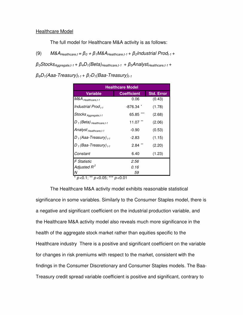
The full model for Healthcare M&A activity is as follows:

(9) M&AHealthcare,t = β0 + β1M&AHealthcare,t-1 + β2Industrial Prodt-1 +

β3StocksAggregate,t-1 + β4D1(Beta)Healthcare,t-1 + β5AnalystHealthcare,t-1 +

β6D1(Aaa-Treasury)t-1 + β7D1(Baa-Treasury)t-1

Healthcare Model

Variable Coefficient Std. Error

M&A Healthcare,t-1 0.06 (0.43)

Industrial Prod t-1 -876.34 * (1.78)

Stocks Aggregate,t-1 65.85 *** (2.68)

D 1 (Beta) Healthcare,t-1 11.07 ** (2.06)

Analyst Healthcare,t-1 -0.90 (0.53)

D 1 (Aaa-Treasury) t-1 -2.83 (1.15)

D 1 (Baa-Treasury) t-1 2.84 ** (2.20)

Constant 6.40 (1.23)

F Statistic 2.56

Adjusted R2

0.16

N 59

* p <0.1; ** p <0.05; *** p <0.01

The Healthcare M&A activity model exhibits reasonable statistical

significance in some variables. Similarly to the Consumer Staples model, there is

a negative and significant coefficient on the industrial production variable, and

the Healthcare M&A activity model also reveals much more significance in the

health of the aggregate stock market rather than equities specific to the

Healthcare industry There is a positive and significant coefficient on the variable

for changes in risk premiums with respect to the market, consistent with the

findings in the Consumer Discretionary and Consumer Staples models. The Baa-

Treasury credit spread variable coefficient is positive and significant, contrary to

my expectation, suggesting that widening credit spreads actually lead to

increased Healthcare M&A activity.

Despite showing reasonable variable significance, the Healthcare M&A

activity model demonstrates poor fit. Healthcare is likely another industry that has

an M&A market strongly motivated by changes in regulation. It is also possible

that Healthcare M&A activity is provoked by some factors unique to the industry,

such as acquiring patents on new drugs, which are largely independent of broad

economic and capital markets factors.

Industrials Model

The full model for Industrials M&A activity is as follows:

(10) M&AIndustrials,t = β0 + β1M&AIndustrials,t-1 + β2Industrial Prodt-1 +

β3StocksAggregate,t-1 + β4D1(Uncertainty)Industrials,t-1 + β5BetaIndustrials,t-1 +

β6D1(Analyst)Industrials,t-1 + β7D1(Aaa-Treasury)t-1 + β8D1(Baa-Treasury)t-1

Industrials Model

Variable Coefficient Std. Error

M&A Industrials,t-1 -0.11 (0.84)

Industrial Prod t-1 -436.22 * (1.74)

Stocks Aggregate,t-1 60.92 *** (4.27)

D 1 (Uncertainty) Industrials,t-1 -0.02 (0.70)

Beta Industrials,t-1 -2.20 (1.26)

D 1 (Analyst) Industrials,t-1 -2.43 (0.91)

D 1 (Aaa-Treasury) t-1 2.22 * (1.72)

D 1 (Baa-Treasury) t-1 -1.11 (1.41)

Constant 1.70 (0.62)

F Statistic 6.29

Adjusted R2

0.43

N 58

* p <0.1; ** p <0.05; *** p <0.01

The Industrials M&A activity model has great fit relative to most other

models, but significance is lacking on many of the variables. Also, note that

StocksAggregate,t-1 has exceptionally high significance, much more than the stock

market variable restricted to Industrials equities, suggesting that Industrials M&A

activity might also be driven more by the health of the aggregate market than its

own. Notably, industrial production is significant in the model of Industrial M&A

activity with a negative coefficient, contradicting my expectation. It is possible

that Industrial M&A activity actually leads industrial production, rather than

lagging it. Consistent with the Healthcare M&A activity model, there is a positive

and significant coefficient on a first differenced credit spread variable, but here it

is the Aaa-Treasury spread. This once again suggests that a widening credit

spread actually leads to increases in M&A activity in the Industrials industry.

Materials Model

The full model for Materials M&A activity is as follows:

(11) M&AMaterials,t = β0 + β1M&AMaterials,t-1 + β2Industrial Prodt-1 +

β3StocksAggregate,t-1 + β4UncertaintyMaterials,t-1 + β5D1(Beta)Materials,t-1 +

β6AnalystMaterials,t-1 + β7Aaa-Treasuryt-1 + β8Baa-Treasuryt-1

Materials Model

Variable Coefficient Std. Error

M&A Materials,t-1 -0.16 (1.26)

Industrial Prod t-1 -458.71 *** (3.54)

Stocks Aggregate,t-1 38.24 *** (4.74)

Uncertainty Materials,t-1 0.01 (0.37)

D 1 (Beta) Materials,t-1 -2.66 * (2.01)

Analyst Materials,t-1 -0.31 (0.60)

Aaa-Treasury t-1 -1.10 ** (2.30)

Baa-Treasury t-1 0.35 (0.87)

Constant 2.85 (1.52)

F Statistic 6.43

Adjusted R2

0.43

N 59

* p <0.1; ** p <0.05; *** p <0.01

The Materials industry M&A activity model produces strong variable

significance in a few variables. With respect to the aggregate stock market health

and industrial production variables, the results align with many of the previous

models. The coefficient on the D1(Beta)Materials,t-1 variable is negative and

significant, suggesting that the materials industry M&A activity decreases after

periods of increasing risk premiums with respect to the market. This is contrary to

the findings in previous models, where the coefficient was positive and

significant. The coefficient on the Aaa-Treasury credit spread variable is negative

and significant, consistent with expectations and a few of the previous models.

Technology Model

The full model for Technology M&A activity is as follows:

(12) M&ATech,t = β0 + β1M&ATech,t-1 + β2Industrial Prodt-1 + β3StocksTech,t-1 +

β4UncertaintyAggregate,t-1 + β5BetaTech,t-1 + β6AnalystTech,t-1 + β7Aaa-Treasuryt-1

Technology Model

Variable Coefficient Std. Error

M&A Tech,t-1 -0.44 *** (3.42)

Industrial Prod t-1 -50.71 (0.12)

Stocks Tech,t-1 222.60 *** (7.05)

Uncertainty Aggregate,t-1 0.06 (1.30)

Beta Tech,t-1 -2.61 (0.77)

Analyst Tech,t-1 -1.83 (0.98)

Aaa-Treasury t-1 -1.99 ** (2.33)

Constant 9.73 (1.27)

F Statistic 14.01

Adjusted R2

0.61

N 59

* p <0.1; ** p <0.05; *** p <0.01

The Technology M&A activity model has fantastic fit relative to most other

models. There is high significance in the lagged dependent variable as well as

the Technology industry stock market variable, suggesting once again that

periods of strong M&A activity are typically unsustainable in the Technology

sector and that M&A activity has a strong positive relationship with Technology

stock prices. The remaining significance is found in the Aaa-Treasury credit

spread, which has a negative coefficient, as expected.

Telecom Model

The full model for Telecom M&A activity is as follows:

(13) M&ATelecom,t = β0 + β1M&ATelecom,t-1 + β2M&ATelecom,t-2 + β3Industrial Prodt-1 +

β4StocksAggregate,t-1 + β5UncertaintyTelecom,t-1 + β6D1(Beta)Telecom,t-1 +

β7D1(Analyst)Telecom,t-1 + β8D1(Aaa-Treasury)t-1 + β9Baa-Treasuryt-1

Telecom Model

Variable Coefficient Std. Error

M&A Telecom,t-1 -0.30 ** (2.43)

M&A Telecom,t-2 -0.22 * (1.70)

Industrial Prod t-1 1485.38 *** (2.82)

Stocks Aggregate,t-1 57.08 ** (2.06)

Uncertainty Telecom,t-1 -0.20 *** (2.88)

D 1 (Beta) Telecom,t-1 -1.07 (0.25)

D 1 (Analyst) Telecom,t-1 6.23 *** (3.49)

D 1 (Aaa-Treasury) t-1 3.38 ** (2.40)

Baa-Treasury t-1 2.22 *** (2.76)

Constant -15.88 *** (4.17)

F Statistic 5.75

Adjusted R2

0.43

N 58

* p <0.1; ** p <0.05; *** p <0.01

The Telecommunications M&A activity model shows tremendous

statistical significance across many variables. Both the first and second lags of

the dependent variable are significant and negative, as expected. Contrary to all

other models, the industrial production variable has a positive and highly

significant coefficient. As expected, the variable for uncertainty in the Telecom

industry has a negative and very significant coefficient. The positive coefficient

on D1(Analyst)Telecom,t-1 suggests that M&A activity in the Telecom industry is

highly driven by changes in analyst expectations, with M&A activity increasing

after analyst expectations increase.

The positive and significant coefficient on the first difference of the Aaa-

Treasury credit spread again suggests that widening credit spreads lead to

increases in M&A activity in the Telecom industry, among other industries.

Interestingly, there is also a positive and significant coefficient on the level of the

Baa-Treasury credit spread. Along with the positive coefficient on the analyst

expectation variable, these results suggest that Telecom M&A activity tends to

boom when default risk in corporations is high relative to the government, with

analysts revising expectations of the future upward. It is possible that this is an

ideal time for Telecom corporations to make large capital investments, potentially

in the form of an M&A transaction.

Utilities Model

The full model for Utilities M&A activity is as follows:

(14) M&AUtilities,t = β0 + β1M&AUtilities,t-1 + β2Industrial Prodt-1 + β3StocksAggregate,t-1

+ β4UncertaintyUtilities,t-1 + β5BetaUtilities,t-1 + β6AnalystUtilities,t-1 +

β7D1(Aaa-Treasury)t-1

Utilities Model

Variable Coefficient Std. Error

M&A Utilities,t-1 -0.13 (0.94)

Industrial Prod t-1 -645.32 *** (2.88)

Stocks Aggregate,t-1 14.88 (1.27)

Uncertainty Utilities,t-1 -0.04 ** (2.11)

Beta Utilities,t-1 -5.32 *** (2.82)

Analyst Utilities,t-1 -0.93 (1.29)

D 1 (Aaa-Treasury) t-1 1.37 ** (2.29)

Constant 11.86 *** (2.90)

F Statistic 4.39

Adjusted R2

0.29

N 59

* p <0.1; ** p <0.05; *** p <0.01

This model shows great significance in many variables. The industrial

production variable shows very strong significance and is negative, consistent

with most previous models. Utilities industry uncertainty is also significant and

negative, suggesting that high uncertainty in the market in one quarter is

detrimental to M&A activity in the next, as expected. The Utilities risk premium

variable is also significant and negative, which suggests increases in risk

premiums in the Utilities industry with respect to the market leads to a decrease

in M&A activity in the Utilities industry. Similarly to some of the previous findings,

it appears that the Utilities industry M&A activity also increases as the spread

between corporate bond yields and treasuries widens.

M&A Activity Drivers Across Industries: Similarities and Differences

For simple comparative purposes, the estimated effects of the proposed

drivers of M&A activity in each industry have been aggregated and organized in

Figure 9, located in Appendix A. As seen in Figure 9, the drivers across each

industry tend to vary in both salience and effect. I will now go through each driver

individually and discuss similarities and differences across industry groups.

Past M&A Activity

Using lags of the dependent variable for each industry showed varying

significance across models, but the estimated effect was consistently negative.

The negative impact of past M&A activity aligns with my expectation and agrees

with the notion that M&A activity has a short-term bursting behavior. It is possible

that this past dependence is due to chain reaction merger activity, where the

merging of two firms provokes competitors to quickly seek out their M&A

opportunities to remain competitive themselves. This would result in short term

bursts in M&A activity in an industry, given the sufficiency of other factors such

as capital liquidity and economic optimism.

The industries in which past M&A activity proved to be most significant

were the Consumer Discretionary, Technology and Telecom industries. It is

possible that these industries exhibit more dependence on past activity due to

unique factors. For the Technology industry, it is possible that new technologies

provoke patent and expertise arms races periodically, triggering bursts in M&A

activity. The Telecom industry potentially has a regulatory component that

triggers a burst in M&A activity, followed quickly by an anti-trust component to

suppress sustained periods of high M&A activity to promote equitable market

shares and restrict pricing power. Notably, past M&A activity is insignificant in the

aggregate model, which contradicts the findings of Barkoulas and Resende, who

separately established that persistence and long-term memory are important

features of M&A activity in the United States and the United Kingdom (Barkoulas

et al., 2001; Resende, 2005).

Industrial Production

For most industries, industrial production was estimated to have a

negative impact on M&A activity, contrary to my primary expectation. Although

high industrial production is a sign of a healthy economy, the likely explanation

for the negative effect is one of timing. As Nelson discovered, industrial

production typically peaks after M&A activity does, so when industrial production

is high in one quarter, it is likely that M&A activity is already decreasing (Nelson,

1959). In the aggregate model, however, industrial production shows no

significance as a driver of M&A activity. The only industry that exhibits industrial

production as a positive driver is Telecom.

The negative significance of industrial production as a driver of M&A

activity was uncovered in the Consumer Staples, Healthcare, Industrials,

Materials and Utilities industries. For the Industrials industry, the reasoning is a

direct connection to Nelson's discovery. The Materials industry provides the raw

inputs for much of the Industrial industry, and the Utilities industry provides

essential services, such as water and electricity, to Industrial consumers. For this

reason, it is likely that these industries' revenue cycles imitate industrial

production, and thus when industrial production is high, the Materials and Utilities

industries are likely healthy and subsequently not as interested in seeking growth

opportunities through mergers and acquisitions.

Stock Market Valuations

As expected, stock market valuation has emerged as a very strong

positive driver of M&A activity, though, interestingly, for some industries the

aggregate stock market health holds more significance than its industry specific

stock market index levels. These results are consistent with the previously

established notion that the stock market tends to lead M&A activity (Nelson,

1959; Melicher et al., 1983) and that stock markets Granger cause M&A activity

(Clarke & Ioannidis, 1996). For the Consumer Discretionary, Financials and

Technology industries, the health of their own industry specific S&P indices were

more significant than the S&P 500 index. This suggests that these industries are

more concerned with the market valuations of their peers than the aggregate

market when making M&A decisions.

Notably, the S&P 500 index is the primary driver of aggregate M&A activity

in the United States, according to my model, holding tremendous significance.

This may indicate that the timing of M&A decisions in the aggregate is primarily

valuation and outlook based. When stock market valuations are high, the market

has an optimistic outlook and corporations are more comfortable making an

acquisition.

Another noteworthy result is that the Energy and Utilities industry models

place no significance on stock market valuations as a driver of M&A activity. For

the Energy industry, it is plausible that the main driver is geologically event

driven, such as the discovery of an abundance of shale or oil in a region already

controlled by another company. As for Utilities, mergers and acquisitions may be

motivated more by the need for geographical diversification and government

regulation, which greatly restricts the amount of expansion opportunities for

Utilities companies, so M&A activity would not be quite as in sync with the stock

market.

Industry Uncertainty

Overall, market uncertainty holds little significance across the models but

exhibits the expected negative effect where significant. The negative relationship

between market uncertainty and M&A activity is consistent with the idea that risk

averse corporations tend to shy away from mergers and acquisitions in the

presence of high uncertainty. This is largely due to enterprise value in an M&A

valuation relying heavily on the ability of the buyer to project the target's future

cash flows, as well as the synergies, to predict value creation of the merger pro-

forma.

The Telecom and Utilities industries are driven in the negative direction by

industry uncertainty, whereas the Consumer Discretionary industry is driven by

the change in aggregate uncertainty. The Consumer Discretionary industry

consists of companies that produce products or provide services that are non-

essential, such as restaurants, vacations, games and new cars. For this reason,

the industry is especially sensitive to the aggregate economic cycles. Signs of

instability are likely looked at more closely because the industry's performance is

highly dependent on the consumer's expectation of the future, causing high

market volatility to act as a red flag.

As discussed in the Description of Data section, the poor performance of

the market uncertainty variables can partially be attributed to the fact that

historical volatilities are a poor proxy of future volatility. Ideally, a forward looking

measure, such as Black-Scholes implied volatility, should be employed, but

sufficient data was not available.

Risk Premiums: Industry Beta

Using the S&P industry indices' market betas as a proxy for the level of

the risk premium in an industry led to significance in several models with mixed

results. For the Materials and Utilities industries, changes in risk premiums and

the level of risk premiums were found to have negative effects on M&A activity,

as I had anticipated. For the Consumer Discretionary, Consumer Staples and

Healthcare industries, however, the effect of changing risk premiums was in fact

positive; an increase in the industry beta in one quarter leads to an increase in

M&A activity in the next. This contradicts my expectation, which was an

adaptation of Haddad's findings that firms with higher exposure to systematic

shocks, or higher market beta, are less likely to be bought out (Haddad et al.,

2011). It is possible that increasing risk premiums in these industries signals the

need for diversification or better growth prospects, and that some firms utilize

M&A as a strong source of inorganic growth and diversification.

Analyst Expectations

As a driver of M&A activity, analyst expectations and changes in

expectations showed little significance in most models. In the Energy and

Telecom models, however, analyst expectations and changes in analyst

expectations emerged as significant, positive drivers of M&A activity, as

expected.

Contrary to the findings of Carapeto, analyst expectations exhibited no

significance in the aggregate model of M&A activity (Carapeto et al., 2010). Part

of the reason is that proxy for analyst expectations, the quarterly change in the

number of buy ratings released by equity analysts, is inappropriate and inherently

flawed. As discussed in the Description of Variables section, analyst coverage

has been increasing greatly over time, as has the number of analysts, which

creates a major, unwanted increase in their proxy for analyst expectations from

quarter to quarter. Although the proxy I created alleviates this issue, another

glaring issue remains: there are very few equities covered for much of the

sample period, and there is a bias towards corporations with high market

capitalization and a history of strong performance. Supporting this claim, the

analyst expectation data series never exhibits an equity rating below 3.12, which

is a slight buy rating, for any quarter in any industry. Further, the average equity

rating over the sample period for each industry hovers around 4, which is a

definite buy. As a result, the analyst expectation variable is a fragmented proxy

and not very representative of the market as a whole. Below, Figure 10 plots the

analyst expectation variables for each industry, and the optimistic bias is

apparent.

Figure 10

Analyst ExpectationsAnalystIndustry

3.0

3.5

4.0

4.5

5.0

1997

1998

1999

2000

2001

2002

2003

2004

2005

2006

2007

2008

2009

2010

2011

Year

Rati

ng

CD CS

Energy Financials

Healthcare Industrials

Materials Technology

Telecom Utilities

Bond Yields

In the models that preferred bond yields to spreads, both Aaa-rated

corporate bond yields and the change in treasury note yields emerged as drivers

of M&A activity. The relationship between bond yields and M&A activity is

negative, consistent with the cost of an acquisition scaling with the cost of capital.

Energy M&A activity responds to Aaa-rated bond yields, and, notably, the

aggregate model also exhibits corporate bond yields as a driver. This is

consistent with the findings of Melicher and Harford but contradicts the early

findings of Beckenstein, who uncovered a positive relationship between M&A

activity and the cost of capital (Beckenstein, 1979; Melicher et al., 1983; Harford,

2005).

Credit Spreads

The effect of credit spreads on M&A activity proved to be a significant

driver in various models, although the results were somewhat mixed. Consistent

with my expectation, the Aaa-Treasury spread was uncovered as a negative

driver of M&A activity in various industries, including Consumer Discretionary,

Materials and Technology. This is likely because wide credit spreads signal

pessimistic outlooks as well as uncertainty in the corporate domain, in addition to

increasing the cost of M&A transactions. The Baa-Treasury spread on the other

hand, was revealed to be a positive driver of M&A transactions in the Consumer

Discretionary and Telecom industries, contrary to my expectation. For the

Consumer Discretionary industry, the net effect of credit spreads as a driver of

M&A is still negative as discussed in the Analysis section, but, interestingly, the

Telecom industry exhibits a net positive relationship. This suggests that the

Telecom industry may actually prefer to make large capital investments while

default risk in corporations is high relative to the United States government.

Surprisingly, the effect of changes in credit spreads was revealed to be a

positive driver of M&A activity in several industries, including Healthcare,

Industrials, Telecom and Utilities. This suggests that a more ideal environment

for M&A transactions in these industries arises when credit spreads are

widening, as investors flee corporate bonds in favor of safer government bonds.

CONCLUSIONS AND SUGGESTIONS FOR FUTURE RESEARCH

The vast domain of M&A drivers research has expanded over time from

broad, aggregate analyses of macroeconomic relationships to more focused

analyses of fundamental and behavioral drivers. Variable treatment and

econometric specifications are inconsistent across published papers, and little

attention has been devoted to how M&A activity drivers vary across industries.

This paper addressed these issues by posing the following question: What drives

mergers and acquisitions activity in each industry in the United States, and how

do those drivers vary across industries? The econometric models developed in

this analysis provided a foothold to tackle this question and establish several

trends.

(i) United States aggregate M&A activity is primarily driven by market valuations

and corporate bond yields, despite the importance of various other drivers at the

industry level. Although industry uncertainty, risk premiums, and other drivers

have shown significance at the industry level, when aggregated together, these

drivers unique to each industry become nearly negligible.

(ii) M&A activity in some industries is highly driven by macroeconomic and

market oriented drivers, whereas others remain largely disconnected from the

macro-economy. Although M&A activity in the Consumer Discretionary,

Industrials, Materials, Technology, and Telecommunications industries is

relatively well explained using macroeconomic and market-oriented drivers, the

Healthcare, Financials and Energy industries are not. These industries must be

driven by other such as changes in regulation and technology, some of which

may be unique to the industry, such as drug patents in the Healthcare industry

and natural resource control in the Energy industry.

(iii) Aggregate stock market valuations drive M&A in many industries, whereas

others are driven by industry specific stock market valuations or are

disconnected. At the aggregate level and in most industries, the health of the

S&P 500 is a positive driver of M&A activity, whereas the Consumer

Discretionary, Financials and Technology industries are driven more by their

industry specific market valuations. The M&A activity of the Energy and Utilities

industries, on the other hand, are not significantly driven by market valuations.

This suggests that Energy and Utilities corporations do not rely heavily on the

stock market to determine whether the environment is ripe for acquisitions, and

that they must be more heavily driven by factors unique to the industries.

(iv) Industry uncertainty is not a significant factor in most industries but drives

M&A activity downward. As expected, industry uncertainty has been uncovered

as a driver of M&A activity in a few industries, with high uncertainty leading to

lower M&A activity. Once again, this is likely due to the fact that pro-forma

analysis and valuation is highly dependent on the predictability of future cash

flows, and risk averse acquirers are less likely to engage in investments with

uncertain payoffs.

(v) Increases in risk premiums preface increased M&A activity in some industries

and decreased activity in others . Contrary to my expectation, increasing risk

premiums in the Consumer Discretionary, Consumer Staples, and Healthcare

industries lead to higher M&A activity. In the Materials and Utilities industries the

effect is negative.

(vi) Analyst expectations do not play a large role in driving M&A activity in most

industries, nor at the aggregate level. Contrary to recent research, analyst

expectations contribute minimally to M&A activity. However, the relationship is

positive in the two industries that significance arose, Energy and Telecom, which

is consistent with previous research, despite the major flaws in the proxy for

analyst expectation that was used in previous papers.

(vii) Aggregate M&A activity is driven downward by high corporate bond yields.

The yields on Aaa-rated corporate bonds has been identified as a primary driver

of aggregate M&A activity, with higher yields leading to depressed M&A activity.\

(viii) M&A activity at the industry level is more reliant on level of credit spreads

rather than bond yields, but the effect is different across industries. In the

Consumer Discretionary, Materials, and Technology industries, higher corporate

credit spreads exhibited a negative impact, whereas the opposite effect was

uncovered in the Telecom industry.

(ix) Widening credit spreads drive stronger M&A activity at the industry level.

Surprisingly, widening credit spreads tend to preface increases in M&A activity in

the Healthcare, Industrials, Telecom, and Utilities industries, despite the

pessimism and increased financing costs associated with widening credit

spreads. In no industry was the opposite effect been revealed with any

significance.

In order to further vet the findings of this paper and contribute further to

the domain of M&A drivers research, important considerations and deviations

from this paper need to be made:

(i) Regulatory and industry specific drivers need to be identified and incorporated

into the models. Some models have reasonable fit as purely forecasting based

models, but there is much room for improvement, and omitted variables bias is

apparent. Some industry models have such poor fit and low variable significance

that it is difficult identify specific drivers of M&A activity, such as with the

Financials industry.

(ii) Forward-looking measures of uncertainty need to be employed. Although

historical volatility has shown significance in the expected direction in some

models, the role of uncertainty cannot be fully captured using historical data.

Forward-looking measures need to be incorporated, such as implied volatility

derived from options prices, which would be a significant improvement if

sufficient data can be obtained.

(iii) Unbiased proxies for analyst expectations need to be used. The proxy for

analyst expectation used in this paper is a definite improvement over past

research, but the variable is still inherently flawed. As I stated previously, there

are very few equities covered for much of the sample period, and there is a bias

towards corporations with high market capitalization and a history of strong

performance. Over time, I suspect this bias to be transient to a certain extent as

analyst coverage improves, but the day that every equity listed on United States

exchanges is covered seems far off. Until then, future research should explore

alternative proxies for analyst expectations.

(iv) Alternative data transformations and variable treatments should be

considered. Although I found more success scaling variables by gross domestic

product than by using levels or taking first differences of logarithmically

transformed data, improvements can almost certainly be made. The main issue

with using first differences of logarithmically transformed quarter M&A volume

data is that the resulting data series is extremely volatile, whereas the

explanatory variables are not, resulting in poor variable significance. Part of the

reasoning behind the high volatility is that M&A volume is highly seasonal from

quarter to quarter. Adjusting for this seasonality or using yearly M&A data in the

specification may result in much better fit and variable significance. Additionally,

lag structures and specifications need to be experimented with more thoroughly

and optimized accordingly.

(v) Use longer sample periods. Much of the data used in this paper extends back

much further than the model sample periods. The reason for this is that the

analyst expectation proxy could only be derived back to the mid-1990s, due to

data insufficiency. If an alternate proxy for analyst expectation is employed, or if

the driver is omitted completely, the models could be estimated over a much

longer time frame and across more varied economic states and conditions.

This research paper represents an initial attempt at identifying the drivers

of M&A activity across industries from a forecasting perspective for comparison

purposes. Improvement of this analysis based on the aforementioned

suggestions would prove useful for forecasting M&A activity in various industries.

If M&A activity can be reliably forecasted, stock price models of investment

banks and other financial institutions that provide financing or advise companies

on mergers and acquisitions could be developed. Similarly, merger arbitrage

could be implemented more reliably in industries that are expected to boom with

M&A activity. This paper, combined with past research and the suggested

refinements, provides an initial step towards the development of such models,

which would prove to be both enlightening and of immense value.

References Andrade, G., Mitchell, M., & Stafford, E. (2001). "New Evidence and Perspectives

on Mergers". Journal of Economic Perspectives, 15(2), 103-120 Barkoulas, J., Baum, C., & Chakraborty, A. (2001). "Waves and persistence in

merger and acquisition activity". Economic Letters, 70, 237-243 Beckenstein, A. (1979). "Merger Activity and Merger Theories: An Empirical

Investigation". The Antitrust Bulletin, 24, 105-128 Boone, A., & Mulherin, J. (2000). "Comparing Acquisitions and Divestitures".

Journal of Corporate Finance, 6, 117-139 Carapeto, M., Dallocchio, M., Faelten, A., Lanzolla, M., & Moeller, S. (2010).

"Can business expectations predict M&A activity?". Retrieved December 2, 2011, from http://www.cass.city.ac.uk/__data/assets/pdf_file/0003/56370/2A_Faelton_Moeller.pdf

Clarke, R., & Ioannidis, C. (1996). "On the relationship between aggregate

merger activity and the stock market: some further empirical evidence". Economic Letters, 53, 349-356

Gärtner, D., & Halbheer, D. (2009). "Are there waves in merger activity after all?".

International Journal of Industrial Organization, 27, 708-718 Golbe, D., & White, L. (1988). "A Time Series Analysis of Mergers and

Acquisitions in the U.S. Economy", in Alan J. Auerbach (ed.), Corporate Takeovers: Causes and Consequences (Chicago: NBER and University of Chicago Press)

Golbe, D., & White, L. (1993). "Catch a Wave: The Time Series Behavior of

Mergers”. The Review of Economics and Statistics, 75(3), (1993), 493-499 Gort, M. (1969). "An Economic Disturbance Theory of Mergers”. The Quarterly

Journal of Economics, 83(4), 624-642 Haddad, V., Loualiche, E., & Plosser, M. (2011). "Buyout Activity and Asset

Prices". Retrieved March 6, 2012, from SSRN: http://papers.ssrn.com/sol3/papers.cfm?abstract_id=1843804

Harford, J. (2005). "What drives merger waves?". Journal of Financial

Economics, 77(3), 529-560

Melicher, R., Ledolter, J., & D'Antonio, L. (1983). "A Time Series Analysis of Aggregate Merger Activity". The Review of Economics and Statistics, 65(3), 423-430

Mitchell, M., & Mulherin, H. (1996). "The impact of industry shocks on takeover

and restructuring activity". Journal of Financial Economics, 41, 193-229 Nelson, R. (1959). "Merger Movements in American Industry, 1895-1956”,

(Princeton: Princeton University Press) Resende, M. (2005). "Mergers and Acquisitions Waves in the U.K.: A Markov-

Switching Approach (EUI Working Paper ECO No. 2005/4)". Retrieved November 28, 2011, from http://cadmus.eui.eu/bitstream/handle/1814/3317/ECO2005-4.pdf

Stughart II, W., & Tollison, R. (1984). "The Random Character of Merger

Activity". The RAND Journal of Economics, 15(4), 500-509 Town, R. (1992). "Merger Waves and the Structure of Merger and Acquisition

Time-Series”. Journal of Applied Econometrics, 7, S83-S100

APPENDIX A

Figure 9

M&A Drivers Across Industries

Explanatory Variable1 Aggregate

Consumer

Discretionary

Consumer

StaplesEnergy Financials Healthcare Industrials Materials Technology Telecom Utilities

M&A Activity

Industrial Production

S&P Industry Index

S&P 500

Industry Uncertainty

Aggregate Uncertainty

∆ Industry Uncertainty

∆ Aggregate Uncertainty

Industry Beta

∆ Industry Beta

Analyst Expectations

∆ Analyst Expectations

Aaa Bond Yields

∆ Aaa Bond Yields

Treasury Note Yields

∆ Treasury Note Yields

Aaa-Treasury Spread

∆ Aaa-Treasury Spread

Baa-Treasury Spread

∆ Baa-Treasury Spread

F Statistic3

8.76 7.19 2.56 2.23 1.56 2.56 6.29 6.43 14.01 5.75 4.39

Adjusted R2 0.48 0.46 0.18 0.14 0.06 0.16 0.43 0.43 0.61 0.43 0.29

N 59 59 58 59 59 59 58 59 59 58 59

1. Variables are one quarter lags, ∆ represents the first difference operator.

2. Green cells indicate positive, statistically significant coefficients. Red cells indicate negative, statistically significant coefficients.

3. Bold indicates statistical significance at the 1% level, red indicates no statistical significance, and the remaining are significant at the 5% level.