Embed Size (px)
Citation preview

Unit Vector Games
Rahul Savani∗ Bernhard von Stengel†
February 15, 2016
Published in: International Journal of Economic Theory 12 (2016), 7–27. doi: 10.1111/ijet.12077
Abstract
McLennan and Tourky (2010) showed that “imitation games” provide a new view of thecomputation of Nash equilibria of bimatrix games with the Lemke–Howson algorithm. Inan imitation game, the payoff matrix of one of the players is the identity matrix. We studythe more general “unit vector games”, which are already known, where the payoff ma-trix of one player is composed of unit vectors. Our main application is a simplificationof the construction by Savani and von Stengel (2006) of bimatrix games where two basicequilibrium-finding algorithms take exponentially many steps: the Lemke–Howson algo-rithm, and support enumeration.
Keywords: bimatrix game, Nash equilibrium computation, imitation game, Lemke–Howson algorithm,unit vector game
1 Introduction
A bimatrix game is a two-player game in strategic form. The Nash equilibria of a bimatrixgame correspond to pairs of vertices of two polyhedra derived from the payoff matrices. Thesevertex pairs have to be “completely labeled”, which expresses the equilibrium condition thatevery pure strategy of a player (represented by a “label”) is either a best response to the otherplayer’s mixed strategy or played with probability zero.
This polyhedral view gives rise to algorithms that compute a Nash equilibrium. A classicalmethod is the algorithm by Lemke and Howson (1964) which follows a path of “almost com-pletely labeled” polytope edges that terminates at Nash equilibrium. The Lemke–Howson (LH)algorithm has been one inspiration for the complexity class PPAD defined by Papadimitriou(1994) of computational problems defined by such path-following arguments, which includesmore general equilibrium problems such as the computation of approximate Brouwer fixed
∗Department of Computer Science, University of Liverpool, Liverpool L69 3BX, United Kingdom. Email:[email protected]
†Department of Mathematics, London School of Economics, London WC2A 2AE, United Kingdom. Email:[email protected]
1
arX
iv:1
501.
0224
3v3
[cs
.GT
] 1
4 Fe
b 20
16

points. An important result proved by Chen and Deng (2006) and Daskalakis, Goldberg, andPapadimitriou (2009) states that every problem in the class PPAD can be reduced to findinga Nash equilibrium of a bimatrix game, which makes this problem “PPAD-complete”. (Theproblem of finding the Nash equilibrium at the end of a specific path is a much harder, namelyPSPACE-complete, see Goldberg, Papadimitriou, and Savani 2013.)
If an algorithm takes exponentially many steps (measured in the size of its input) for certainproblem instances, these are considered “hard” instances for the algorithm. Savani and vonStengel (2006) constructed bimatrix games that are hard instances for the LH algorithm. Theirconstruction uses “dual cyclic polytopes” which have a well-known vertex structure for anydimension and number of linear inequalities. Morris (1994) used similarly labeled dual cyclicpolytopes where all “Lemke paths” are exponentially long. A Lemke path is related to the pathcomputed by the LH algorithm, but is defined on a single polytope that does not have a productstructure corresponding to a bimatrix game. The completely labeled vertex found by a Lemkepath can be interpreted as a symmetric equilibrium of a symmetric bimatrix game. However,as in the example in Figure 4 below, such a symmetric game may also have nonsymmetricequilibria which here are easy to compute, so that the result by Morris (1994) seemed unsuitableto describe games that are hard to solve with the LH algorithm.
The “imitation games” defined by McLennan and Tourky (2010) changed this picture. In animitation game, the payoff matrix of one of the players is the identity matrix. The mixed strategyof that player in any Nash equilibrium of the imitation game corresponds exactly to a symmetricequilibrium of the symmetric game defined by the payoff matrix of the other player. In that way,an algorithm that finds a Nash equilibrium of a bimatrix game can be used to find a symmetricNash equilibrium of a symmetric game. (The converse statement that a bimatrix game can be“symmetrized”, see Proposition 2 below, is an earlier folklore result stated for zero-sum gamesby Gale, Kuhn, and Tucker 1950.)
In one sense the two-polytope construction of Savani and von Stengel (2006) was overly com-plicated: the imitation games by McLennan and Tourky (2010) provide a simple and elegantway to turn the single-polytope construction of Morris (1994) into exponentially-long LH pathsfor bimatrix games. In another sense, the construction of Savani and von Stengel was not redun-dant. Namely, the square imitation games obtained from Morris (1994) have a single completelymixed equilibrium that is easily computed by equating all payoffs for all pure strategies. Savaniand von Stengel (2006) extended their construction of square games with long LH paths (anda single completely mixed equilibrium) to non-square games that are simultaneously hard forthe LH algorithm and “support enumeration”, which is another natural and simple algorithm forfinding equilibria. The support of a mixed strategy is the set of pure strategies that are playedwith positive probability. Given a pair of supports of equal size, the mixed strategy probabilitiesare found by equating all payoffs for the other player’s support, which then have to be comparedwith payoffs outside the support to establish the equilibrium property (see Dickhaut and Kaplan1991).
In this paper, we extend the idea of imitation games to games where one payoff matrix is ar-bitrary and the other is a set of unit vectors. We call these unit vector games. An imitationgame is an example of a unit vector game, where the unit vectors form an identity matrix. Themain result of this paper is an application of unit vector games: we use them to extend Morris’s
2

construction to obtain non-square bimatrix games that use only one dual cyclic polytope, ratherthan the two used by Savani and von Stengel, and which are simultaneously hard both for theLH algorithm and support enumeration. This result (Theorem 11) was first described by Savani(2006, Section 3.8).
Before presenting this construction in Section 3, we introduce in Section 2 the required back-ground on labeled best response polytopes for bimatrix games, in an accessible presentation dueto Shapley (1974) that we think every game theorist should know. We define unit vector gamesand the use of imitation games, and their relationships to the LH algorithm. We will make thecase that unit vector games provide a general and simple way to construct bimatrix games usinga single labeled polytope.
To our knowledge, unit vector games were first defined and used by Balthasar (2009, Lemma4.10) in a different context, namely in order to prove that a symmetric equilibrium of a non-degenerate symmetric game that has positive “symmetric index” can be made the unique sym-metric equilibrium of a larger symmetric game by adding suitable strategies (Balthasar 2009,Theorem 4.1).
2 Unit vector games
In this section, we first describe in Section 2.1 how labeled polyhedra capture the “best-responseregions” of mixed strategies where a particular pure strategy of the other player is a best re-sponse, and how these are used to identify Nash equilibria. In Section 2.2 we introduce unitvector games, whose equilibria correspond to completely labeled vertices of a single labeledpolytope. In Section 2.3 we discuss the role of imitation games for symmetric games and theirsymmetric equilibria. Finally, in Section 2.4, we show how Lemke paths defined for single la-beled polytopes are “projections” of seemingly more general LH paths in the case of unit vectorgames (Theorem 5).
2.1 Nash equilibria of bimatrix games and polytopes
Consider an m× n bimatrix game (A,B). We describe a geometric-combinatorial “labeling”method, due to Shapley (1974), that allows an easy identification of the Nash equilibria of thegame. It has an equivalent description in terms of polytopes derived from the payoff matrices.
Let 0 be the all-zero vector and let 1 be the all-one vector of appropriate dimension. All vectorsare column vectors and C> is the transpose of any matrix C, so 1> is the all-one row vector.Let X and Y be the mixed-strategy simplices of the two players,
X = {x ∈ Rm | x≥ 0, 1>x = 1}, Y = {y ∈ Rn | y≥ 0, 1>y = 1}. (1)
It is convenient to identify the m+n pure strategies of the two players by separate labels wherethe labels 1, . . . ,m denote the m pure strategies of the row player 1 and the labels m+ 1, . . . ,m+n denote the n pure strategies of the column player 2.
Consider mixed strategies x ∈ X and y ∈ Y . We say that x has label m+ j for 1≤ j ≤ n if j isa pure best response of player 2 to x. Similarly, y has label i for 1 ≤ i ≤ m if i is a pure bestresponse of player 1 to y. In addition, we say that x has label i for 1≤ i≤ m if xi = 0, and that
3

y has label m+ j for 1≤ j ≤ n if y j = 0. That is, a mixed strategy such as x has label i (one ofthe player’s own pure strategies) if i is not played.
In a Nash equilibrium, every pure strategy that is played with positive probability is a bestresponse to the other player’s mixed strategy. In other words, if a pure strategy is not a bestresponse, it is played with probability zero. Hence, a mixed strategy pair (x,y) is a Nashequilibrium if and only if every label in {1, . . . ,m+n} appears as a label of x or of y. The Nashequilibria are therefore exactly those pairs (x,y) in X ×Y that are completely labeled in thissense.
As an example, consider the 3×3 game (A,B) with
A =
1 0 00 1 00 0 1
, B =
0 2 43 2 00 2 0
. (2)
The labels 1,2,3 represent the pure strategies of player 1 and 4,5,6 those of player 2. Figure 1shows X and Y with these labels shown as circled numbers. The interiors of these triangles arecovered by best-response regions labeled by the other player’s pure strategies, which are closedpolyhedral sets where the respective pure strategy is a best response. For example, the best-response region in Y with label 1 is the set of those (y1,y2,y3) such that y1 ≥ y2 and y1 ≥ y3 ,due to the particularly simple form of A in (2). The outsides of X and Y are labeled with theplayers’ own pure strategies where these are not played. These outside facets are opposite tothe vertex where only that pure strategy is played; for example, label 1 is the label of the facetof X opposite to the vertex (1,0,0). In Figure 1 there is only one pair (x,y) that is completelylabeled, namely x = (1
3 ,23 ,0) with labels 3,4,5 and y = (1
2 ,12 ,0) with labels 1,2,6, so this is the
only Nash equilibrium of the game.
64
5
2 1
3(1,0,0) (0,1,0)
(0,0,1)
x
3
1 2
6
4
5
(1,0,0) (0,1,0)
(0,0,1)
y
Figure 1 Labeled mixed strategy sets X and Y for the game (2).
The subdivision of X and Y into best-response regions is most easily seen with the help ofthe “upper envelope” of the payoffs to the other player, which are defined by the followingpolyhedra. Let
P = {(x,v) ∈ X×R | B>x≤ 1v}, Q = {(y,u) ∈ Y ×R | Ay≤ 1u}. (3)
For the example (2), the inequalities B>x≤ 1v state that 3x2 ≤ v, 2x1+2x2+2x3 ≤ v, 4x1 ≤ v,which say that v is at least the best-response payoff to player 2. If one of these inequalities
4

is tight (holds as equality), then v is exactly the best-response payoff to player 2. The left-hand diagram in Figure 2 shows these “best-response facets” of P, and their projection to X byignoring the payoff variable v, which defines the subdivision of X into best-response regions asin the left-hand diagram in Figure 1.
(0,0,1)
(1,0,0) (0,1,0)
v
5
61
0
2
3
4 4
3
2
1
0
0
2
3
4
1
4
(0,0,0)
1x 2x
3x
5
6
4
Figure 2 Best-response facets of the polyhedron P in (3), and the polytope P in (4), for thegame in (2).
Throughout this paper, assume (without loss of generality) that A and B> are non-negative andhave no zero column. Then v and u in B>x≤ 1v and Ay≤ 1u are always positive. By dividingthese inequalities by v and u, respectively, and writing xi instead of xi/v and y j instead of y j/u,the polyhedra P and Q are replaced by P and Q,
P = {x ∈ Rm | x≥ 0, B>x≤ 1}, Q = {y ∈ Rn | Ay≤ 1, y≥ 0}, (4)
which are bounded and therefore polytopes. For B in (2), P is shown on the right in Figure 2.
Both polytopes P and Q in (4) are defined by m+ n inequalities that correspond to the purestrategies of the player, which we have denoted by the labels 1, . . . ,m+n. We can now identifythe labels, as pure best responses of the other player, or unplayed own pure strategies, as tightinequalities in either polytope. That is, a point x in P has label k if the kth inequality in P istight, that is, if xk = 0 for 1≤ k≤m or (B>x)k−m = 1 for m+1≤ k≤m+n. Similarly, y in Qhas label k if (Ay)k = 1 for 1≤ k≤m or yk−m = 0 for m+1≤ k≤m+n. Then (x,y) in P×Qis completely labeled if x and y together have all labels in {1, . . . ,m+ n}. With the exceptionof (0,0), these completely labeled points of P×Q represent (after rescaling to become pairs ofmixed strategies) exactly the Nash equilibria of the game (A,B).
The pair (x,y) in P×Q is completely labeled if
xi = 0 or (Ay)i = 1 for all i = 1, . . . ,m, y j = 0 or (B>x) j = 1 for all j = 1, . . . ,n. (5)
Because x, 1−Ay, y, and 1−B>x are all non-negative, the complementarity condition (5) canalso be stated as the orthogonality condition
x>(1−Ay) = 0, y>(1−B>x) = 0. (6)
The characterization of Nash equilibria as completely labeled pairs (x,y) holds for arbitrarybimatrix games. For considering algorithms, it is useful to assume that the game is nondegen-erate in the sense that no point in P has more than m labels, and no point in Q has more than
5

n labels. Clearly, for a nondegenerate game, in an equilibrium (x,y) each label appears exactlyonce either as a label of x or of y.
Nondegeneracy is equivalent to the condition that the number of pure best responses against amixed strategy is never larger than the size of the support of that mixed strategy. It implies thatP is a simple polytope in the sense that no point of P lies on more than m facets, and similarlythat Q is a simple polytope. A facet is obtained by turning one of the inequalities that define thepolytope into an equality, provided that the inequality is irredundant, that is, cannot be omittedwithout changing the polytope. A redundant inequality in the definition of P and Q may alsogive rise to a degeneracy if it corresponds to a pure strategy that is weakly (but not strictly)dominated by, or payoff equivalent to, a mixture of other strategies. For a detailed discussionof degeneracy see von Stengel (2002).
2.2 Unit vector games and a single labeled polytope
The components of the kth unit vector ek are 0 except for the kth component, which is 1. Inan m× n unit vector game (A,B), every column of A is a unit vector in Rm . The matrix B isarbitrary, and without loss of generality B> is non-negative and has no zero column.
In this subsection, we consider such a unit vector game (A,B). Let the jth column of A bethe unit vector e`( j) , for 1 ≤ j ≤ n. Then the sequence `(1), . . . , `(n) together with the payoffmatrix B completely specifies the game.
For this game, the polytope Q in (4) has a very special structure. For 1≤ i≤ m, let
Ni = { j | `( j) = i, 1≤ j ≤ n} (7)
so that Ni is the set of those columns j whose best response is row i. These sets Ni are pairwisedisjoint, and their union is {1, . . . ,n}. Then clearly
Q = {y ∈ Rn | ∑j∈Ni
y j ≤ 1, 1≤ i≤ m, y≥ 0}. (8)
That is, except for the order of inequalities, Q is the product of m simplices of the form {z ∈RNi |∑ j∈Ni z j ≤ 1, z≥ 0}, for 1≤ i≤m. If each Ni is a singleton, then, by (7), A is a permutedidentity matrix, n = m, each simplex is the unit interval, and Q is the n-dimensional unit cube.
In any bimatrix game, the polytopes P and Q in (4) each have m+n inequalities that correspondto the pure strategies of the two players. Turning the kth inequality into an equality typicallydefines a facet of the polytope, which defines the label k of that facet, 1≤ k ≤ m+n.
In our unit vector game (A,B) where the jth column of A is the unit vector e`( j) , for 1≤ j ≤ n,we introduce the labeled polytope P` ,
P` = {x ∈ Rm | x≥ 0, B>x≤ 1}, (9)
where the m+n inequalities of P` have the labels i for the first m inequalities xi≥ 0, 1≤ i≤m,and the jth inequality of B>x≤ 1 has label `( j), for 1≤ j ≤ n. That is, P` is just the polytopeP in (4) except that the last n inequalities are labeled with `(1), . . . , `(n), each of which is anumber in {1, . . . ,m}. A point x of P` is completely labeled if every number in {1, . . . ,m}
6
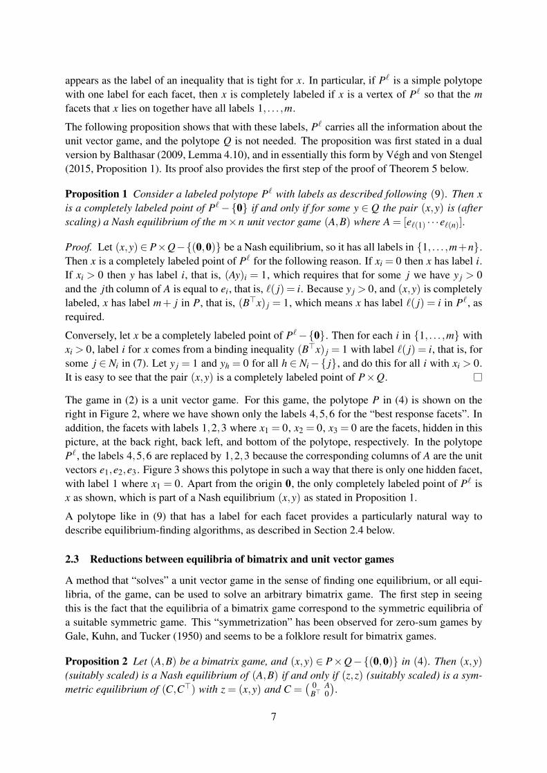
appears as the label of an inequality that is tight for x. In particular, if P` is a simple polytopewith one label for each facet, then x is completely labeled if x is a vertex of P` so that the mfacets that x lies on together have all labels 1, . . . ,m.
The following proposition shows that with these labels, P` carries all the information about theunit vector game, and the polytope Q is not needed. The proposition was first stated in a dualversion by Balthasar (2009, Lemma 4.10), and in essentially this form by Vegh and von Stengel(2015, Proposition 1). Its proof also provides the first step of the proof of Theorem 5 below.
Proposition 1 Consider a labeled polytope P` with labels as described following (9). Then xis a completely labeled point of P`−{0} if and only if for some y ∈ Q the pair (x,y) is (afterscaling) a Nash equilibrium of the m×n unit vector game (A,B) where A = [e`(1) · · ·e`(n)].
Proof. Let (x,y)∈ P×Q−{(0,0)} be a Nash equilibrium, so it has all labels in {1, . . . ,m+n}.Then x is a completely labeled point of P` for the following reason. If xi = 0 then x has label i.If xi > 0 then y has label i, that is, (Ay)i = 1, which requires that for some j we have y j > 0and the jth column of A is equal to ei , that is, `( j) = i. Because y j > 0, and (x,y) is completelylabeled, x has label m+ j in P, that is, (B>x) j = 1, which means x has label `( j) = i in P` , asrequired.
Conversely, let x be a completely labeled point of P`−{0}. Then for each i in {1, . . . ,m} withxi > 0, label i for x comes from a binding inequality (B>x) j = 1 with label `( j) = i, that is, forsome j ∈ Ni in (7). Let y j = 1 and yh = 0 for all h ∈ Ni−{ j}, and do this for all i with xi > 0.It is easy to see that the pair (x,y) is a completely labeled point of P×Q.
The game in (2) is a unit vector game. For this game, the polytope P in (4) is shown on theright in Figure 2, where we have shown only the labels 4,5,6 for the “best response facets”. Inaddition, the facets with labels 1,2,3 where x1 = 0, x2 = 0, x3 = 0 are the facets, hidden in thispicture, at the back right, back left, and bottom of the polytope, respectively. In the polytopeP` , the labels 4,5,6 are replaced by 1,2,3 because the corresponding columns of A are the unitvectors e1,e2,e3 . Figure 3 shows this polytope in such a way that there is only one hidden facet,with label 1 where x1 = 0. Apart from the origin 0, the only completely labeled point of P` isx as shown, which is part of a Nash equilibrium (x,y) as stated in Proposition 1.
A polytope like in (9) that has a label for each facet provides a particularly natural way todescribe equilibrium-finding algorithms, as described in Section 2.4 below.
2.3 Reductions between equilibria of bimatrix and unit vector games
A method that “solves” a unit vector game in the sense of finding one equilibrium, or all equi-libria, of the game, can be used to solve an arbitrary bimatrix game. The first step in seeingthis is the fact that the equilibria of a bimatrix game correspond to the symmetric equilibria ofa suitable symmetric game. This “symmetrization” has been observed for zero-sum games byGale, Kuhn, and Tucker (1950) and seems to be a folklore result for bimatrix games.
Proposition 2 Let (A,B) be a bimatrix game, and (x,y) ∈ P×Q−{(0,0)} in (4). Then (x,y)(suitably scaled) is a Nash equilibrium of (A,B) if and only if (z,z) (suitably scaled) is a sym-metric equilibrium of (C,C>) with z = (x,y) and C =
( 0 AB> 0
).
7

x
0
2
311
3
2
Figure 3 The polytope P` for the unit vector game (2). The hidden facet at the back haslabel 1, written on the left.
Proof. This holds by (6) because (z,z) is an equilibrium of (C,C>) if and only if z 6= 0, z≥ 0,Cz≤ 1, and z>(1−Cz) = 0.
By Proposition 2, finding an equilibrium of a bimatrix game can be reduced to finding a sym-metric equilibrium of a symmetric bimatrix game. The converse follows from the followingproposition, due to McLennan and Tourky (2010, Proposition 2.1), with the help of imitationgames. They define an imitation game as an m×m bimatrix game (A,B) where B is the identitymatrix. Here, we define an imitation game as a special unit vector game (A,B) where A (ratherthan B) is the identity matrix I . The reason for this (clearly not very material) change is thatthis game is completely described by the polytope P` in (9), which corresponds to P in (4)and compared to Q has a more natural description because the m inequalities x≥ 0 with labels1, . . . ,m are listed first.
Proposition 3 The pair (x,x) is a symmetric Nash equilibrium of the symmetric bimatrix game(C,C>) if and only if (x,y) is a Nash equilibrium of the imitation game (I,C>) for some y.
6
3
4
5
2 1
(1,0,0) (0,1,0)
(0,0,1)
x
b
a
3
6
1
2
5 4
(1,0,0) (0,1,0)
(0,0,1)
x
b
a
Figure 4 Labeled mixed-strategy sets X and Y for the symmetric game (C,C>) in (10).
As an example, consider the symmetric game (C,C>) with
C =
0 3 02 2 24 0 0
, C> =
0 2 43 2 00 2 0
, (10)
8

so that C> = B in (2). Figure 4 shows the labeled mixed-strategy simplices X and Y for thisgame. In addition to the symmetric equilibrium (x,x) where x = (1
3 ,23 ,0), the game has two
non-symmetric equilibria (a,b) and (b,a) where a = (12 ,
12 ,0) and b = (0, 2
3 ,13). A method
that just finds a Nash equilibrium of a bimatrix game may not find a symmetric equilibriumwhen applied to this game, which shows the use of Proposition 3. The corresponding imitationgame (I,C>) is just (A,B) in (2), which has the unique equilibrium (x,y) where (x,x) is thesymmetric equilibrium of (C,C>).
31
2
2 1
3(1,0,0) (0,1,0)
(0,0,1)
x
1
3
3
12
2
(0,0,1)
(1,0,0) (0,1,0)x
Figure 5 (Left) Best-response regions for identifying symmetric equilibria. (Right) Degener-ate symmetric game (11) with a unique symmetric equilibrium.
The left-hand diagram in Figure 5 shows the mixed strategy simplex X subdivided into regionsof pure best responses against the mixed strategy itself, which corresponds to the polytope P`
in Figure 3. The (in this case unique) symmetric equilibrium is the completely labeled point x.
The right-hand diagram in Figure 5 shows this subdivision of X for another game (C,C>) where
C =
0 4 02 2 24 0 0
, C> =
0 2 44 2 00 2 0
. (11)
This game is degenerate because the mixed strategy x = (12 ,
12 ,0) has three pure best responses.
This mixed strategy x also defines the unique symmetric equilibrium (x,x) of this game. How-ever, the corresponding equilibria (x,y) of the imitation game (I,C>) are not unique, becausedue to the degeneracy any convex combination of (1
2 ,12 ,0) and (1
3 ,13 ,
13) can be chosen for y, as
shown in Figure 6.
Hence the reduction between symmetric equilibria (x,x) of a symmetric game and Nash equilib-ria (x,y) of the corresponding imitation game stated in Proposition 3 does not preserve unique-ness if the game is degenerate.
2.4 Lemke paths and Lemke–Howson paths
Consider a labeled polytope P` as in (9). We assume throughout that P` is nondegenerate, thatis, no point of P` has more than m labels. Therefore, P` is a simple polytope, and every tightinequality defines a separate facet (we can omit inequalities that are never tight), each of whichhas a label in {1, . . . ,m}. The path-following methods described in this section can be extendedto degenerate games and polytopes; for an exposition see von Stengel (2002).
9

4
3
6
12
5
(0,0,1)
(1,0,0) (0,1,0)x
3
1 2
4
5
6(1,0,0) (0,1,0)
(0,0,1)
y
Figure 6 Labeled mixed-strategy sets for the imitation game (I,C>) for the degenerate sym-metric game (11) where the equilibria (x,y) are not unique.
A Lemke path is a path that starts at a completely labeled vertex of P` such as 0 and ends atanother completely labeled vertex. It is defined by choosing one label k in {1, . . . ,m} that isallowed to be missing. After this choice of k, the path proceeds in a unique manner from thestarting point. By leaving the facet with label k, a unique edge is traversed whose endpoint isanother vertex, which lies on a new facet. The label, say j, of that facet, is said to be picked up.If this is the missing label k, then the path terminates at a completely labeled vertex. Otherwise,j is clearly duplicate and the next edge is uniquely chosen by leaving the facet that so far hadlabel j, and the process is repeated. The resulting path consists of a sequence of k-almostcomplementary edges and vertices (so defined by having all labels except possibly k, where koccurs only at the starting point and endpoint of the path). The path cannot revisit a vertexbecause this would offer a second way to proceed when that vertex is first encountered, whichis not the case because P` is nondegenerate. Hence, the path terminates at another completelylabeled vertex of P` (which is a Nash equilibrium of the corresponding unit vector game inProposition 1 if the path starts at 0). Figure 7 shows an example.
x
0
2
311
3
2
Figure 7 Lemke path for missing label 1 for the polytope in Figure 3.
For a fixed missing label k, every completely labeled vertex of P` is a separate endpoint of aLemke path. Because each path has two endpoints, there is an even number of them, and all ofthese except 0 are Nash equilibria of the unit vector game, so the number of Nash equilibria isodd.
10
This path-following method was first described by Lemke (1965) in order to find a solutionto a linear complementarity problem (LCP); it is normally described for polyhedra, not forpolytopes, so that termination requires additional assumptions (see Cottle, Pang, and Stone1992). The standard description of an LCP assumes a square matrix B with labels `( j) = j forj = 1, . . . ,m. Allowing P` to have m+ n rather than 2m facets with individual labels `( j) forthe last n facets corresponds to a generalized LCP (sometimes also called “vertical LCP”), asstudied in Cottle and Dantzig (1970). The term “Lemke paths” for polytopes is due to Morris(1994).
The algorithm by Lemke and Howson (1964) finds one Nash equilibrium of an m×n bimatrixgame (A,B). Let C =
( 0 AB> 0
)as in Proposition 2. Then one way to define a Lemke–Howson
(LH) path for missing label k in {1, . . . ,m+ n} is as a Lemke path for missing label k for thelabeled polytope
R` = {z ∈ Rm+n | z≥ 0, Cz≤ 1} (12)
where the 2(m+n) inequalities of R` have labels 1, . . . ,m+n,1, . . . ,m+n (that is, `(i) = i fori = 1, . . . ,m+n).
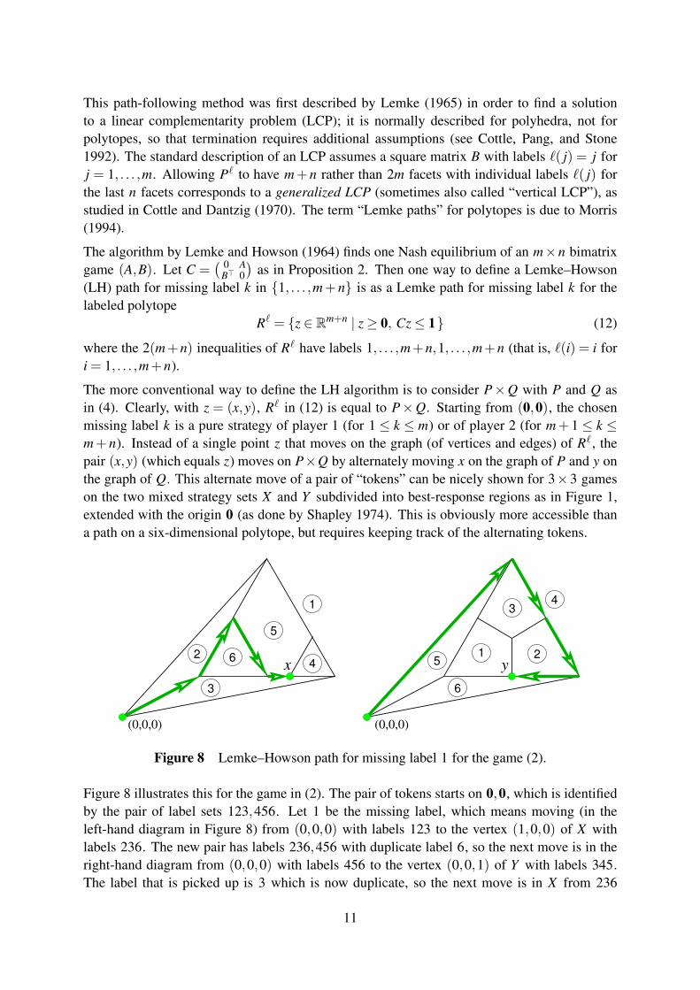
The more conventional way to define the LH algorithm is to consider P×Q with P and Q asin (4). Clearly, with z = (x,y), R` in (12) is equal to P×Q. Starting from (0,0), the chosenmissing label k is a pure strategy of player 1 (for 1 ≤ k ≤ m) or of player 2 (for m+ 1 ≤ k ≤m+ n). Instead of a single point z that moves on the graph (of vertices and edges) of R` , thepair (x,y) (which equals z) moves on P×Q by alternately moving x on the graph of P and y onthe graph of Q. This alternate move of a pair of “tokens” can be nicely shown for 3×3 gameson the two mixed strategy sets X and Y subdivided into best-response regions as in Figure 1,extended with the origin 0 (as done by Shapley 1974). This is obviously more accessible thana path on a six-dimensional polytope, but requires keeping track of the alternating tokens.
64
5
1
3
2
3
1 2
4
5
6
(0,0,0) (0,0,0)
x y
Figure 8 Lemke–Howson path for missing label 1 for the game (2).
Figure 8 illustrates this for the game in (2). The pair of tokens starts on 0,0, which is identifiedby the pair of label sets 123,456. Let 1 be the missing label, which means moving (in theleft-hand diagram in Figure 8) from (0,0,0) with labels 123 to the vertex (1,0,0) of X withlabels 236. The new pair has labels 236,456 with duplicate label 6, so the next move is in theright-hand diagram from (0,0,0) with labels 456 to the vertex (0,0,1) of Y with labels 345.The label that is picked up is 3 which is now duplicate, so the next move is in X from 236
11

to 256. Then 5 is duplicate, with a move in Y from 345 to 234. With 2 duplicate, the nextmove in X is from 256 to 356. Then 3 is duplicate, moving in Y from 234 to 246. Then 6 isduplicate, moving in X from 356 to 345, which is the point x = (1
3 ,23 ,0). Then 4 is duplicate,
moving in Y from 246 to 126, which is the point y = (12 ,
12 ,0) which has the missing label 1.
This terminates the LH path for missing label 1 at the Nash equilibrium (x,y).
The two diagrams in Figure 8 show two separate paths on P and Q, respectively (representedby X and Y subdivided into best-response regions). These paths are traversed in alternate stepsand define a single path on the product polytope P×Q. In general, a simple path on P×Q (thatis, a path that does not revisit a vertex) may not “project” to simple paths on P and Q. However,for LH paths this is the case, as stated in the following proposition (Lemma 2.3 of Savani 2006,and implicit in McLennan and Tourky 2010, Section 4).
Proposition 4 Every LH path on P×Q induces a simple path in each polytope P and Q, thatis, no vertex of P or Q is ever left and visited again on an LH path.
Proof. Suppose to the contrary that a vertex x of P is left and visited again on an LH path. Thismeans that there are three vertex pairs (x,y), (x,y′), and (x,y′′) of P×Q, with pairwise distinctvertices y, y′ , and y′′ of Q, on an LH path with missing label k, say. All three pairs have alllabels except possibly k. The m labels of x define n−1 labels shared by y, y′ , and y′′ . However,this is impossible, since these n−1 labels correspond to n−1 equations in Rn that define a line,which can only contain two vertices of Q. The same reasoning applies to a vertex y of Q thatwould be visited multiple times on an LH path.
Consider an m× n unit vector game (A,B) where A = [e`(1) · · ·e`(n)]. According to Propo-sition 1, the labeled polytope P` carries all information about the Nash equilibria of (A,B).Recall that P` is the polytope P in (4) but where the labels m+ j for the strategies j of thecolumn player, 1≤ j ≤ n, are replaced by `( j), that is, by the best responses of the row playerto these columns. Replacing these labels in the left-hand diagram in Figure 1 gives the left-handdiagram in Figure 5, equivalent to P` in Figure 3,
We now establish the same correspondence with regard to the LH paths on P×Q for the game(A,B), where the corresponding “projection” to P defines a Lemke path on P` . For example,the LH path projected to P shown in the left-hand diagram in Figure 8 is the same as the Lemkepath on P` in Figure 7. Both paths are defined for the missing label 1. It seems natural thatthe LH path for missing label i in {1, . . . ,m} projects to the Lemke path for missing label ion P` . However, there are n additional LH paths for the game (A,B) for the missing labelsm+ j for j in {1, . . . ,n}, which do not exist as labels of P` . The following theorem statesthat these project to the Lemke paths on P` for the missing label `( j). This generalizes thecorresponding assertion by McLennan and Tourky (2010, p. 9) and Savani and von Stengel(2006, Proposition 15) for imitation games where `( j) = j.
Theorem 5 Consider an m× n unit vector game (A,B) where A = [e`(1) · · ·e`(n)], with P` asin (9) and P and Q as in (4). Then the LH path on P×Q for this game for missing label kprojects to a path on P that is the Lemke path on P` for missing label k if 1≤ k ≤ m, and thatis the Lemke path for missing label `( j) if k = m+ j for 1≤ j ≤ n.
12

Proof. In Proposition 1 it was shown that the completely labeled pairs (x,y) of P×Q corres-pond to the completely labeled points x of P` . It is easy to see that if P is nondegenerate, asassumed here, then this correspondence is one-to-one, and x and y are vertices.
In the following, i is always an element of {1, . . . ,m}, and j is always an element of {1, . . . ,n}.Consider a step of an LH path on P×Q that leaves or arrives at a vertex x of P, as part of a pair(x,y). If the dropped label is i, then xi = 0 changes to xi > 0, and if the dropped label is m+ j,then (B>x) j = 1 changes to (B>x) j < 1. If i is a label that is picked up, then xi > 0 changes toxi = 0, and if m+ j is a label that is picked up, then (B>x) j < 1 changes to (B>x) j = 1.
Similarly, consider a vertex y of Q. Because Q is a product of m simplices as in (8), for eachi the following holds: either y j = 0 for all j ∈ Ni , or for exactly one j ∈ Ni we have y j = 1(which means (Ay)i = 1 and y has label `( j) = i) and yh = 0 for all h ∈ Ni−{ j}. We can alsodescribe precisely which label is picked up after moving away from y by dropping a label:
(a) If the dropped label is i, then y j = 1 (for some j ∈ Ni) changes to y j = 0, so that m+ j isthe label that is picked up.
(b) If the dropped label is m+ j, this is just the reverse step: j ∈ Ni for a unique i = `( j), soy j = 0 changes to y j = 1, which means i = `( j) is the label that is picked up.
Consider now steps on an LH path with missing label k, and assume that any label that ispicked up is not the missing label k, and therefore duplicate. Suppose label i is picked up in P,corresponding to the binding inequality xi = 0. Label i is duplicate and therefore dropped in Q.By (a), this means that m+ j with j ∈ Ni is picked up in Q, where i = `( j). The duplicate labelm+ j in P corresponds to the binding inequality (B>x) j = 1. So the next step is to move awayfrom this facet in P. In P` this same facet with (B>x) j = 1 has label `( j) = i, and moving awayfrom this facet is exactly the next step on the Lemke path on P` .
Similarly, suppose label m+ j is picked up in P, which corresponds to the facet (B>x) j = 1which in P` has label i = `( j). On the LH path, the duplicate label m+ j in Q is dropped as in(b), where label i is picked up in Q and therefore duplicate. In P, the facet with this duplicatelabel is given by xi = 0. The next step on the LH path is to move away from this facet, which isthe same facet from which the Lemke path on P` moves away.
Similar considerations apply when the LH path is started or terminates. If the missing label is kin {1, . . . ,m}, then the LH path starts by dropping k in P, and the Lemke path starts in the sameway in P` . When the LH path terminates by picking up the missing label k in P, the Lemkepath ends in the same way in P` . If it terminates by picking up the missing label k in Q, thenby (b) this was preceded by dropping the previously duplicate label m+ j where j ∈ Nk , that is,after the path reached in P the facet defined by (B>x) j = 1 which has label `( j) = k in P` , sothe Lemke path has already terminated on P` .
The LH path with missing label k = m+ j starts by dropping this label in Q. By (b), the labelthat is picked up in Q is `( j), which is now duplicate, and the path proceeds by dropping thislabel in P which is the same as starting the Lemke path on P` with this missing label. The LHpath terminates by picking up the missing label k = m+ j in P by reaching the facet definedby (B>x) j = 1 which has label `( j), so that the Lemke path on P` terminates. Alternatively,label k = m+ j is picked up in Q which by (a) was preceded by dropping label i = `( j), which
13

was duplicate because it was picked up in P when encountering the facet xi = 0, where i is themissing label `( j) on the Lemke path that has therefore terminated on P` .
3 Hard-to-solve bimatrix games
With the help of Theorem 5, it suffices to construct suitable labeled polytopes with (exponen-tially) long Lemke paths in order to show that certain games have long LH paths. McLennanand Tourky (2010) (summarized in Savani and von Stengel 2006, Section 5) showed with thehelp of imitation games that the polytopes with long Lemke paths due to Morris (1994) can beused for this purpose. In this section we extend this construction, with the help of unit vectorgames, to games that are not square and that are hard to solve not only with the Lemke–Howsonalgorithm, but also with support enumeration methods.
In Section 3.1 we present a very simple model of random games that have very few Nashequilibria on average, unlike games where all payoffs are chosen at random. These games areunit vector games, and the result (Proposition 6) is joint work with Andy McLennan. We thendescribe in Section 3.2 dual cyclic polytopes, whose facets have a nice combinatorial structure,which have proved useful for the construction of games with many equilibria, and with long LHpaths. Our main result, Theorem 11 in Section 3.3, describes unit vector games based on dualcyclic polytopes whose equilibria are hard to find not only with the LH algorithm, but also withsupport enumeration.
3.1 Permutation games
We present here a small “warmup” result that was found jointly with Andy McLennan. Apermutation game is an n×n game (A,B) where A is the identity matrix and B is a permutedidentity matrix, that is, the ith row of B is the unit vector e>
π(i) for some permutation π of{1, . . . ,n} (so column π(i) is the best response to row i, and, because A = I , the best responseto column j is row j). Let Iπ be this matrix B, so that the permutation game is (I, Iπ).
Because a permutation game (I, Iπ) is an imitation game, the two strategies in an equilibriumhave equal support. It is easy to see that any equilibrium of (I, Iπ) is of the form (x,x) where xmixes uniformly over its support S where S is any nonempty subset of {1, . . . ,n} that is closedunder π , that is, i ∈ S implies π(i) ∈ S. In other words, S is any nonempty union of cycles of π .
A very simple model of a “random” game is to consider a permutation game (I, Iπ) for a randompermutation π .
Proposition 6 A random n×n permutation game has in expectation n Nash equilibria.
Proof. Consider a random permutation π of {1, . . . ,n}. Let E(n) be the expected number ofNash equilibria of (I, Iπ), where we want to prove that E(n) = n, which is true for n = 1. Letn > 1 and assume as inductive hypothesis that the claim is true for n−1. With probability 1
n wehave π(n) = n, in which case π defines also a random permutation of {1, . . . ,n− 1}, and anyequilibrium of (I, Iπ) is either the pure strategy equilibrium where both players play n, or anequilibrium with a support S of a random (n−1)×(n−1) permutation game, or an equilibrium
14

with support S∪{n}. Hence, in this case the number of equilibria of (I, Iπ) is twice the numberE(n−1) of equilibria of a random (n−1)×(n−1) game plus one. Otherwise, with probabilityn−1
n , we have π(n) 6= n, so that π defines a random permutation of {1, . . . ,n−1} when removingn from the cycle of π that contains n. For any equilibrium of the (n−1)× (n−1) permutationgame whose support contains this cycle, we add n back to the cycle to obtain the respectiveequilibrium of the n× n game. So in the case π(n) 6= n the expected number of equilibria isE(n−1). That is,
E(n) =1n(1+2 ·E(n−1))+
n−1n
E(n−1) =1n(1+2(n−1)+(n−1)(n−1)) = n,
which completes the induction.
Random permutation games have very few equilibria, as Proposition 6 shows. In contrast,McLennan and Berg (2005) have shown that the expected number of equilibria of an n× ngame with random payoffs is exponential in n. Barany, Vempala, and Vetta (2007) show thatsuch a game has with high probability an equilibrium with small support. A permutation game(I, Iπ), where the permutation π has k cycles, has 2k− 1 many equilibria, but a large numberk of cycles is rare. In fact, there are (n− 1)! single-cycle permutations, so with probability1/n = (n− 1)!/n! the permutation game has only a single equilibrium with full support. Forsuch games, an algorithm that enumerates all possible supports starting with those of small sizetakes exponential time. On the other hand, it is easy to see that the LH algorithm finds anequilibrium in the shortest possible time, because it just adds the strategies in a cycle of π to itscurrent support.
However, a square game has only one full support, which is natural to test as to whether itdefines a (completely mixed) equilibrium. The full support always defines an equilibrium ina permutation game. It also does for the square games described by Savani and von Stengel(2006) which have exponentially long LH paths. They therefore constructed also non-squaregames where support enumeration takes exponentially long time on average. It is an openquestion whether non-square games can be constructed from unit vectors as an extension ofpermutation games that are also hard to solve with support enumeration.
3.2 Cyclic polytopes and Gale evenness bitstrings
With the polytopes P and Q in (4), Nash equilibria of bimatrix games correspond to completelylabeled points of P×Q. The “dual cyclic polytopes” have the property that they have themaximal possible number of vertices for a given dimension and number of facets (see Ziegler1995, or Grunbaum 2003). In addition, it is easy to describe each vertex by the facets it lieson. Using these polytopes, von Stengel (1999) constructed counterexamples for n ≥ 6 to aconjecture by Quint and Shubik (1997) that a nondegenerate n× n game has at most 2n− 1equilibria. McLennan and Park (1999) proved this conjecture for n = 4; the case n = 5 is stillopen. Morris (1994) gave a construction of labeled dual cyclic polytopes with exponentiallylong Lemke paths, which we extend in Theorem 11 below.
A standard way to define a cyclic polytope P ′ in dimension m with f vertices is as the convexhull of f points µ(t j) on the moment curve µ : t 7→ (t, t2, . . . , tm)> for 1≤ j ≤ f . However, the
15

polytopes in (4) are defined by inequalities and not as convex hulls of points. In the dual (or“polar”) of a polytope, its vertices are reinterpreted as normal vectors of facets. The polytopeP ′ is first translated so that it has the origin 0 in its interior, for example by subtracting thearithmetic mean µ of the points µ(t j) from each such point. The resulting vectors µ(t j)− µ
then define the dual cyclic polytope in dimension m with f facets
Cmf = {x ∈ Rm | (µ(t j)−µ)>x≤ 1, 1≤ j ≤ f }. (13)
A suitable affine transformation of Cmf (see von Stengel 1999, p. 560) gives a polytope P as
in (4) or (9) so that the first m inequalities of P have the form x ≥ 0. The last n = f −minequalities B>x≤ 1 of P then determine the m×n payoff matrix B. If the first m inequalitieshave labels 1, . . . ,m and the last n inequalities have labels `(1), . . . , `(n), then this defines alabeled polytope P` as in (9) and a unit vector game as in Proposition 1.
A vertex u of Cmf is characterized by the bitstring u1u2 · · ·u f of length f , where the jth bit u j
indicates whether u is on the jth facet (u j = 1) or not (u j = 0). The polytope is simple, soexactly m bits are 1, and the other f −m bits are 0. Assume (which is all that is needed) thatt1 < t2 < · · ·< t f when defining the jth facet of Cm
f by the binding inequality (µ(t j)−µ)>x = 1in (13). As shown by Gale (1963), the vertices of Cm
f are characterized by the bitstrings thatfulfill the Gale evenness condition: A bitstring with exactly m 1s represents a vertex if andonly if in any substring of the form 01s0 the number s of 1s is even, so it has no odd-lengthsubstrings of the form 010, 01110, and so on (the reason is that the two zeros ui = u j = 0at the end of such an odd-length substring would represent two points µ(ti) and µ(t j) on themoment curve that are on opposite sides of the hyperplane through the points µ(tk) for uk = 1,so that this hyperplane cannot define a facet of the cyclic polytope that is the convex hull of allthe points, and therefore does not correspond to a vertex of the dual cyclic polytope). Initialsubstrings 1s0 and terminal substrings 01t are allowed to have an odd number s or t of 1s. Weonly consider even dimensions m, where s and t can only be both odd and by a cyclic shift(“wrapping around”) of the bitstring define an even-length substring 01t1s0, which shows thecyclic symmetry of the Gale evenness condition.
Consider, for even m, the bitstrings of length f with m 1s that fulfill Gale evenness, and asbefore let n = f −m. One such string is 1m0n , that is, m 1s followed by n 0s. For the cor-responding vertex of Cm
f , the first m inequalities are tight, and if we label them with 1, . . . ,m,then this defines the completely labeled vertex that is mapped to 0 in the affine map from Cm
f
to the polytope P, which will be a labeled polytope P` . The last n facets of P` correspond tothe last n positions of the bitstring, and they have labels `(1), . . . , `(n). If we view ` as a string`(1) · · ·`(n) of n labels, each of which is an element of {1, . . . ,m}, then these labels specify alabeled polytope. A completely labeled vertex corresponds to a Gale evenness bitstring u1 . . .u fwith f = m+ n where the positions i so that ui = 1 have all m labels, the label being i if1≤ i≤m, and `( j) if i = m+ j for 1≤ j ≤ n. We call the resulting polytope Cm
` , so this is thedual cyclic polytope Cm
f where f = m+n and n is the length of the string ` of the last n facetlabels, mapped affinely to P` as in (9), with facet labels as described.
16

3.3 Triple Morris games
In the notation just introduced, Morris (1994) studied Lemke paths on the labeled dual cyclicpolytope Cm
σ , which we call the Morris polytope, for a string σ of m labels defined as follows.Let τ be the string τ(1) · · ·τ(m) of m labels, which is 1324 for m = 4, 132546 for m = 6,13254768 for m = 8, and in general defined by
τ(1) = 1, τ(i) = i+(−1)i (2≤ i≤ m−1), τ(m) = m, (14)
and let σ be the string τ in reverse order, that is,
σ(i) = τ(m− i+1) (1≤ i≤ m), (15)
so σ = 4231 for m = 4, σ = 645231 for m = 6, σ = 86745231 for m = 8, and so on. We definethe triple Morris polytope as Cm
στσ , where the concatenated string στσ is a string of 3m labels,for example 645231132546645231 if m = 6.
1 2 3 4 5 6 6 4 5 2 3 1
v1 1 1 1 1 1 · · · · · ·· 1 1 1 1
v1
v
1 · · · · ·· 1 1
v1 1 · 1
v
1 · · · ·· 1 1 · 1
v
1v1 1 · · · ·
· 1 1 ·v1 1 · 1
v
1 · · ·· 1 1 · ·
v1
v
1 1 1 · · ··
v1 1 · · · 1 1 1
v
1 · ·· · 1 1 · · 1
v1 1 1 · ·
· · 1 1 ·v
1v1 · 1 1 · ·
· · 1 1v
1 1 · ·v1 1 · ·
· · 1 1 1 1 · · · 1v
1 ·· · · 1 1
v1
v
1 · · 1 1 ·· · ·
v1 1 · 1 1 · 1 1 ·
· · · · 1v
1v1 1 · 1 1 ·
· · · ·v1 1 · 1
v
1 1 1 ·· · · · ·
v1
v
1 1 1 1 1 ·· · · · · · 1 1 1 1 1
v
1
1 2 3 4 5 6 6 4 5 2 3 1 1 3 2 5 4 6 6 4 5 2 3 1
v1 1 1 1 1 1 · · · · · · · · · · · · · · · · · ·· 1 1 1 1
v1
v
1 · · · · · · · · · · · · · · · · ·· 1 1
v1 1 · 1
v
1 · · · · · · · · · · · · · · · ·· 1 1 · 1
v
1v1 1 · · · · · · · · · · · · · · · ·
· 1 1 ·v1 1 · 1
v
1 · · · · · · · · · · · · · · ·· 1 1 · ·
v1
v
1 1 1 · · · · · · · · · · · · · · ··
v1 1 · · · 1 1 1
v
1 · · · · · · · · · · · · · ·· · 1 1 · · 1
v1 1 1 · · · · · · · · · · · · · ·
· · 1 1 ·v
1v1 · 1 1 · · · · · · · · · · · · · ·
· · 1 1v
1 1 · ·v1 1 · · · · · · · · · · · · · ·
· · 1 1 1 1 · · · 1v
1 · · · · · · · · · · · · ·· · · 1 1
v1
v
1 · · 1 1 · · · · · · · · · · · · ·· · ·
v1 1 · 1 1 · 1 1 · · · · · · · · · · · · ·
· · · · 1v
1v1 1 · 1 1 · · · · · · · · · · · · ·
· · · ·v1 1 · 1
v
1 1 1 · · · · · · · · · · · · ·· · · · ·
v1
v
1 1 1 1 1 · · · · · · · · · · · · ·· · · · · · 1 1 1 1 1
v
1 · · · · · · · · · · · ·
Figure 9 Lemke paths for missing label 1 on the Morris polytope C6σ (left), and on the triple
Morris polytope C6στσ (right).
The left-hand diagram of Figure 9 shows the Lemke path for missing label 1 on the Morrispolytope Cm
σ for m = 6. The top row gives the labels, where the first m are the labels 1, . . . ,mcorresponding to the inequalities x ≥ 0 in P` , followed by the labels 645231 of σ . The rowsbelow show the vertices of C6
σ as bitstrings, where bit 1 is written in a different font and 0 as adot · to distinguish them better. The first string 111111000000 represents the starting vertex 0 ofP` . A facet that is left by dropping a label, at first the missing label 1, has a small “v” underneaththe bit 1, whereas the facet that is just encountered, with the corresponding label that is pickedup, has the “v” above it. Dropping label 1 means the second vertex is 011111100000, wherelabel 6 is picked up and duplicate. Because the previous facet with that label corresponds to
17
the second to last bit 1, it is dropped next, which gives the next vertex as 011110110000 wherelabel 4 is picked up, and so on.
The right-hand diagram in Figure 9 shows the Lemke path for missing label 1 on the tripleMorris polytope C6
στσ . Because in this case the only affected bits are those with labels in thefirst substring σ of the entire label string στσ , the path is essentially the same as in the Morrispolytope C6
σ on the left.
1 2 3 4 5 6 6 4 5 2 3 11 1 1
v1 1 1 · · · · · ·
v1 1 1 · 1 1 · · · · ·
v
1· 1
v1 · 1 1 · · · ·
v
1 1v
1 1 · · 1 1 · · · · 1v1
1v1 · · 1 1 · · ·
v
1 1 ·v1 · · · 1 1 · · · 1 1
v
1· · · ·
v1 1 · ·
v
1 1 1 1· · · · ·
v1
v
1 · 1 1 1 1· · · · · · 1
v
1 1 1 1 1
1 2 3 4 5 6 6 4 5 2 3 1 1 3 2 5 4 6 6 4 5 2 3 11 1 1
v1 1 1 · · · · · · · · · · · · · · · · · ·
v1 1 1 · 1 1 · · · · · · · · · · · · · · · · ·
v
1
· 1v1 · 1 1 · · · · · · · · · · · · · · · ·
v
1 1v
1 1 · · 1 1 · · · · · · · · · · · · · · · · 1v1
1v1 · · 1 1 · · · · · · · · · · · · · · ·
v
1 1 ·1 · · · 1 1 · · · · · · · · · · · · · · · 1 1
v
1
· · · ·v1 1 · · · · · · · · · · · · · ·
v
1 1 1 1
· · · · ·v1
v
1 · · · · · · · · · · · · · 1 1 1 1
· · · · · · 1v
1 · · · · · · · · · · · · 1 1 1 1
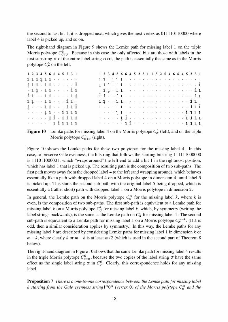
Figure 10 Lemke paths for missing label 4 on the Morris polytope C6σ (left), and on the triple
Morris polytope C6στσ (right).
Figure 10 shows the Lemke paths for these two polytopes for the missing label 4. In thiscase, to preserve Gale evenness, the bitstring that follows the starting bitstring 111111000000is 111011000001, which “wraps around” the left end to add a bit 1 in the rightmost position,which has label 1 that is picked up. The resulting path is the composition of two sub-paths. Thefirst path moves away from the dropped label 4 to the left (and wrapping around), which behavesessentially like a path with dropped label 4 on a Morris polytope in dimension 4, until label 5is picked up. This starts the second sub-path with the original label 5 being dropped, which isessentially a (rather short) path with dropped label 1 on a Morris polytope in dimension 2.
In general, the Lemke path on the Morris polytope Cmσ for the missing label k, where k is
even, is the composition of two sub-paths. The first sub-path is equivalent to a Lemke path formissing label k on a Morris polytope Ck
σ for missing label k, which, by symmetry (writing thelabel strings backwards), is the same as the Lemke path on Ck
σ for missing label 1. The secondsub-path is equivalent to a Lemke path for missing label 1 on a Morris polytope Cm−k
σ . (If k isodd, then a similar consideration applies by symmetry.) In this way, the Lemke paths for anymissing label k are described by considering Lemke paths for missing label 1 in dimension k orm− k, where clearly k or m− k is at least m/2 (which is used in the second part of Theorem 8below).
The right-hand diagram in Figure 10 shows that the same Lemke path for missing label 4 resultsin the triple Morris polytope C6
στσ , because the two copies of the label string σ have the sameeffect as the single label string σ in C6
σ . Clearly, this correspondence holds for any missinglabel.
Proposition 7 There is a one-to-one correspondence between the Lemke path for missing labelk starting from the Gale evenness string1m0m (vertex 0) of the Morris polytope Cm
σ and the
18

Lemke path for missing label k starting from the Gale evenness string 1m03m (vertex 0) of thetriple Morris polytope Cm
στσ , for 1≤ k ≤ m.
The length of the Lemke path for missing label 1 on Cmσ is exponential in the dimension m.
Essentially, this path composed of two such paths in dimension m−2, with another such pathin dimension m− 4 between them (Figure 9 gives an indication). Hence, if the length of thepath is am , the recurrence am = 2am−2 + am−4 implies that it grows from am−2 to am by anapproximate factor of 1+
√2; for details see Morris (1994), and for similar arguments Savani
and von Stengel (2006, Theorem 7). Recall that Θ( f (n)) means bounded above and below bya constant times f (n) for large n.
Theorem 8 (Morris 1994, Proposition 3.4) The longest Lemke path on Cmσ is for missing label 1
and has length Θ((1+√
2)m/2). The shortest Lemke path on Cmσ is for missing label m/2 and
has length Θ((1+√
2)m/4).
Consequently, the Lemke paths on triple Morris polytopes are also exponentially long. Hence,these polytopes define unit vector games which by Theorem 5 have exponentially long LHpaths. We consider these games because they are of dimension m× 3m rather than m×m forthe unit vector game defined by the Morris polytope Cm
σ . The latter, square game has a singlecompletely mixed equilibrium, which is easily found by support enumeration. We show nextthat the m× 3m game has multiple equilibria, each of them with full support for player 1 (forwhich we need the “middle” label string τ ).
Proposition 9 The m× 3m unit vector game that corresponds to the triple Morris polytopeCm
στσ has 3m/2 Nash equilibria. Each of them has full support for player 1.
σ τ σ
1 2 3 4 5 6 6 4 5 2 3 1 1 3 2 5 4 6 6 4 5 2 3 11 0 0 0
1 1 0 0 0 0 0 01 1 1 0 0 0 0 0 0 0 0 0
1 1 1 1 0 0 0 0 0 0 0 0 0 0 0 01 1 1 1 1 0 0 0 0 0 0 0 0 0 0 0 0 0 0 0
1 1 1 1 1 1 0 0 0 0 0 0 0 0 0 0 0 0 0 0 0 0 0 0
(a) 0 0 1 00 0 0 0 1 1 0 0
(b) 0 0 0 0 0 1 0 1 1 0 0 00 0 0 0 0 0 1 1 0 0 1 1 0 0 0 0
(c) 0 0 0 0 0 0 0 1 1 0 1 0 0 1 1 0 0 0 0 00 0 0 0 0 0 0 0 1 1 0 0 1 1 0 0 1 1 0 0 0 0 0 0
Figure 11 Illustration of the proof of Proposition 9 for m = 6. The top half shows the onlycompletely labeled bitstring u = 1m03m where um = 1, the bottom half one suchstring where um = 0. There are three choices in each of the m/2 lines (a), (b), (c).
19
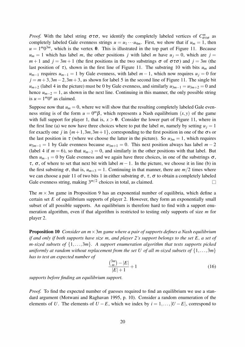
Proof. With the label string στσ , we identify the completely labeled vertices of Cmστσ as
completely labeled Gale evenness strings u = u1 · · ·u4m . First, we show that if um = 1, thenu = 1m03m , which is the vertex 0. This is illustrated in the top part of Figure 11. Becauseum = 1 which has label m, the other positions j with label m have u j = 0, which are j =m+ 1 and j = 3m+ 1 (the first positions in the two substrings σ of στσ ) and j = 3m (thelast position of τ ), shown in the first line of Figure 11. The substring 10 with bits um andum−1 requires um−1 = 1 by Gale evenness, with label m− 1, which now requires u j = 0 forj = m+3,3m−2,3m+3, as shown for label 5 in the second line of Figure 11. The single bitum+2 (label 4 in the picture) must be 0 by Gale evenness, and similarly u3m−1 = u3m+2 = 0 andhence um−2 = 1, as shown in the next line. Continuing in this manner, the only possible stringis u = 1m0n as claimed.
Suppose now that um = 0, where we will show that the resulting completely labeled Gale even-ness string is of the form u = 0mβ , which represents a Nash equilibrium (x,y) of the gamewith full support for player 1, that is, x > 0. Consider the lower part of Figure 11, where inthe first line (a) we now have three choices where to put the label m, namely by setting u j = 1for exactly one j in {m+1,3m,3m+1}, corresponding to the first position in one of the σ s orthe last position in τ (where we choose the latter in the picture). So u3m = 1, which requiresu3m−1 = 1 by Gale evenness because u3m+1 = 0. This next position always has label m− 2(label 4 if m = 6), so that um−2 = 0, and similarly in the other positions with that label. Butthen um−1 = 0 by Gale evenness and we again have three choices, in one of the substrings σ ,τ , σ , of where to set that next bit with label m− 1. In the picture, we choose it in line (b) inthe first substring σ , that is, um+3 = 1. Continuing in that manner, there are m/2 times wherewe can choose a pair 11 of two bits 1 in either substring σ , τ , σ to obtain a completely labeledGale evenness string, making 3m/2 choices in total, as claimed.
The m× 3m game in Proposition 9 has an exponential number of equilibria, which define acertain set E of equilibrium supports of player 2. However, they form an exponentially smallsubset of all possible supports. An equilibrium is therefore hard to find with a support enu-meration algorithm, even if that algorithm is restricted to testing only supports of size m forplayer 2.
Proposition 10 Consider an m×3m game where a pair of supports defines a Nash equilibriumif and only if both supports have size m, and player 2’s support belongs to the set E , a set ofm-sized subsets of {1, . . . ,3m}. A support enumeration algorithm that tests supports pickeduniformly at random without replacement from the set U of all m-sized subsets of {1, . . . ,3m}has to test an expected number of (3m
m
)−|E|
|E|+1+1 (16)
supports before finding an equilibrium support.
Proof. To find the expected number of guesses required to find an equilibrium we use a stan-dard argument (Motwani and Raghavan 1995, p. 10). Consider a random enumeration of theelements of U . The elements of U −E , which we index by i = 1, . . . , |U−E|, correspond to
20

non-equilibrium supports. Let Wi be the indicator variable that takes value 1 if the ith ele-ment of U−E precedes all members of E in the enumeration of U , and 0 otherwise. ThenW = ∑
|U−E|i=1 Wi is the random variable equal to the number of supports checked before the first
equilibrium is found. For a single element of U −E , the probability that it is in front of allelements of E is 1/(|E|+1). Hence, using the linearity of expectation,
E(W ) = E(|U−E|
∑i=1
Wi) =|U−E|
∑i=1
E(Wi) =|U−E|
∑i=1
1|E|+1
=|U |− |E||E|+1
=
(3mm
)−|E|
|E|+1.
This shows that the expected number of support guesses until an equilibrium is found is givenby (16), as claimed.
In Proposition 10, we assume that the algorithm does not identify any particular pattern as towhich supports should be tested. One way to achieve this is to permute the columns of thegame randomly (if one knows that the payoff matrix B of player 2 is derived from a dual cyclicpolytope, then this random order can be identified with a specialized method, see Savani 2006,Section 3.6; this is not a general method for solving games so we do not consider it). However,unless one distorts the polytope Q in (8), this still leaves a payoff matrix of player 1 where eachunit vector appears three times. In this case, even if the algorithm picks only columns whereeach unit vector appears once, there would be 3m possible supports which define a set U of size3m rather than
(3mm
)in Proposition 10. Such a set U is still exponentially large compared to the
set E of 3m/2 supports that define a Nash equilibrium. In that case the expected time for thesupport-testing algorithm in the following theorem is (
√3)m ≈ 1.732m .
Theorem 11 Finding a Nash equilibrium of the m× 3m unit-vector game that correspondsto the triple Morris polytope Cm
στσ takes at least time Θ((1+√
2)m/4) ≈ Θ(1.246m) with theLemke–Howson algorithm, and on expectation time Θ((27/4
√3)m/√
m) ≈ Θ(3.897m/√
m)
with an algorithm that tests in random order arbitrary supports of size m×m of the game.
Proof. The length of the LH paths follows from Theorem 8, Proposition 7, and Theorem 5. Forthe support-testing algorithm, we have |E|= (
√3)m in Proposition 10 by Proposition 9. Using
Stirling’s formula n! ∼√
2πn · (n/e)n , we have(3m
m
)∼ (√
3 · 33m)/(2√
πm · 22m), so that theexpression in (16) is Θ((27/4
√3)m/√
m).
To conclude, we note results on the following combinatorial problem: Let m be even and let `be a string of n labels from {1, . . . ,m}, and consider the set of Gale evenness bitstrings of lengthm+ n which encode the vertices of the labeled polytope Cm
` . The problem is to find a secondcompletely labeled Gale evenness string other than 1m0n . Casetti, Merschen, and von Stengel(2010) have shown that this is equivalent to finding a second perfect matching in the Euler graphwith nodes 1, . . . ,m and edges defined by the Euler tour 1, . . . ,m, `(1), . . . , `(n),1. The edgesin a perfect matching encode the pairs of 1s in a Gale evenness bitstring, which is completelylabeled because the edges cover all nodes. Vegh and von Stengel (2015, Theorem 12) givea near-linear time algorithm that finds such a second perfect matching that, in addition, hasopposite sign, which corresponds to a Nash equilibrium of positive index as it would be foundby a Lemke path (which, however, can be exponentially long). So this combinatorial problemis simpler than the problem of finding a Nash equilibrium of a bimatrix game, even though itgives rise to games that are hard to solve by the standard methods considered in Theorem 11.
21
Acknowledgements
The first author was supported by EPSRC grant EP/L011018/1. We thank the referees forhelpful comments.
ReferencesBalthasar, A. V. (2009), Geometry and Equilibria in Bimatrix Games, PhD Thesis, London School of
Economics.Barany, I., S. Vempala, and A. Vetta (2007), “Nash equilibria in random games,” Random Structures and
Algorithms 31, 391–405.Casetti, M. M., J. Merschen, and B. von Stengel (2010), “Finding Gale strings,” Electronic Notes in
Discrete Mathematics 36, 1065–1072.Chen, X., and X. Deng (2006), “Settling the complexity of two-player Nash equilibrium,” Proc. 47th
Symp. Foundations of Computer Science (FOCS), 261–272.Cottle, R. W., and G. B. Dantzig (1970), “A generalization of the linear complementarity problem,” J.
Combinatorial Theory 8, 79–90.Cottle, R. W., J.-S. Pang, and R. E. Stone (1992), The Linear Complementarity Problem. Academic Press,
San Diego.Daskalakis, C., P. W. Goldberg, and C. H. Papadimitriou (2009), “The complexity of computing a Nash
equilibrium,” SIAM Journal on Computing 39, 195–259.Dickhaut, J., and T. Kaplan (1991), “A program for finding Nash equilibria,” The Mathematica Journal
1, Issue 4, 87–93.Gale, D. (1963), “Neighborly and cyclic polytopes,” V. Klee, ed., Convexity, Proc. Seventh Symposium
in Pure Mathematics, Vol. 7, 225–232, Providence, Rhode Island: American Mathematical Society.Gale, D., H. W. Kuhn, and A. W. Tucker (1950), “On symmetric games,” H. W. Kuhn and A. W. Tucker,
eds., Contributions to the Theory of Games I, Annals of Mathematics Studies 24, 81–87, Princeton:Princeton University Press.
Goldberg, P. W., C. H. Papadimitriou, and R. Savani (2013), “The complexity of the homotopy method,equilibrium selection, and Lemke–Howson solutions,” ACM Transactions on Economics and Com-putation 1, Article 9.
Grunbaum, B. (2003), Convex Polytopes, 2nd ed., Graduate Texts in Mathematics, Vol. 221, New York:Springer.
Lemke, C. E. (1965), “Bimatrix equilibrium points and mathematical programming,” Management Sci-ence 11, 681–689.
Lemke, C. E., and J. T. Howson, Jr. (1964), “Equilibrium points of bimatrix games,” Journal of theSociety for Industrial and Applied Mathematics 12, 413–423.
McLennan, A., and J. Berg (2005), “Asymptotic expected number of Nash equilibria of two-player nor-mal form games,” Games and Economic Behavior 51, 264–295.
McLennan, A., and I.-U. Park (1999), “Generic 4×4 two person games have at most 15 Nash equilibria,”Games and Economic Behavior 26, 111–130.
McLennan, A., and R. Tourky (2010), “Imitation games and computation,” Games and Economic Be-havior 70, 4–11.
Morris, W. D., Jr. (1994), “Lemke paths on simple polytopes,” Mathematics of Operations Research 19,780–789.
Motwani, R., and P. Raghavan (1995), Randomized Algorithms, Cambridge: Cambridge University Press.
22

Papadimitriou, C. H. (1994), “On the complexity of the parity argument and other inefficient proofs ofexistence,” Journal of Computer and System Sciences 48, 498–532.
Quint, T., and M. Shubik (1997), “A theorem on the number of Nash equilibria in a bimatrix game,”International Journal of Game Theory 26, 353–359.
Savani, R. (2006), Finding Nash Equilibria of Bimatrix Games, PhD Thesis, London School of Eco-nomics.
Savani, R., and B. von Stengel (2006), “Hard-to-solve bimatrix games,” Econometrica 74, 397–429.Shapley, L. S. (1974), “A note on the Lemke–Howson algorithm,” Mathematical Programming Study 1:
Pivoting and Extensions, 175–189.Vegh, L. A., and B. von Stengel (2015), “Oriented Euler complexes and signed perfect matchings,”
Mathematical Programming Series B 150, 153–178.von Stengel, B. (1999), “New maximal numbers of equilibria in bimatrix games,” Discrete and Compu-
tational Geometry 21, 557–568.von Stengel, B. (2002), “Computing equilibria for two-person games,” R. J. Aumann and S. Hart, eds.,
Handbook of Game Theory, Vol. 3, 1723–1759, Amsterdam: North-Holland.Ziegler, G. M. (1995), Lectures on Polytopes. Graduate Texts in Mathematics, Vol. 152, New York:
Springer.
23