Unit roots and cointegration in panels

Jörg Breitung(University of Bonn and Deutsche Bundesbank)

M. Hashem Pesaran(Cambridge University)

Discussion PaperSeries 1: Economic StudiesNo 42/2005Discussion Papers represent the authors’ personal opinions and do not necessarily reflect the views of theDeutsche Bundesbank or its staff.

Editorial Board: Heinz Herrmann Thilo Liebig Karl-Heinz Tödter Deutsche Bundesbank, Wilhelm-Epstein-Strasse 14, 60431 Frankfurt am Main, Postfach 10 06 02, 60006 Frankfurt am Main Tel +49 69 9566-1 Telex within Germany 41227, telex from abroad 414431, fax +49 69 5601071 Please address all orders in writing to: Deutsche Bundesbank, Press and Public Relations Division, at the above address or via fax +49 69 9566-3077

Reproduction permitted only if source is stated.

ISBN 3–86558–105–6

Abstract:

This paper provides a review of the literature on unit roots and cointegrationin panels where the time dimension (T ), and the cross section dimension(N) are relatively large. It distinguishes between the first generation testsdeveloped on the assumption of the cross section independence, and thesecond generation tests that allow, in a variety of forms and degrees, thedependence that might prevail across the different units in the panel. In theanalysis of cointegration the hypothesis testing and estimation problems arefurther complicated by the possibility of cross section cointegration whichcould arise if the unit roots in the different cross section units are due tocommon random walk components.

JEL Classification: C12, C15, C22, C23.

Keywords: Panel Unit Roots, Panel Cointegration, Cross Section Dependence,Common Effects

Nontechnical Summary

This paper provides a review of the theoretical literature on testing for unitroots and cointegration in panels where the time dimension (T ), and thecross section dimension (N) are relatively large. In cases where N is large(say over 100) and T small (less than 10) the analysis can proceed only un-der restrictive assumptions such as dynamic homogeneity and/or local crosssection dependence as in spatial autoregressive or moving average models.In cases where N is small (less than 10) and T is relatively large standardtime series techniques applied to systems of equations, such as the SeeminglyUnrelated Regression Equations (SURE), can be used and the panel aspectof the data should not pose new technical difficulties.

Testing the unit root and cointegration hypotheses by using panel datainstead of individual time series involves several additional complications.First, panel data generally introduce a substantial amount of unobservedheterogeneity, rendering the parameters of the model cross section specific.Second, in many empirical applications it is inappropriate to assume that thecross section units are independent. To overcome these difficulties, variantsof panel unit root tests are developed that allow for different forms of crosssectional dependence. Third, the panel test outcomes are often difficult tointerpret if the null of the unit root or cointegration is rejected. Fourth, withunobserved nonstationary common factors affecting some or all the variablesin the panel, it is also necessary to consider the possibility of cointegrationbetween the variables across the groups (cross section cointegration) as wellas within group cointegration. Finally, the asymptotic theory is considerablymore complicated due to the fact that the sampling design involves a timeas well as a cross section dimension. Furthermore, a proper limit theory hasto take into account the relationship between the increasing number of timeperiods and cross section units.

By comparison to panel unit root tests, the analysis of cointegration inpanels is still at an early stages of its developments. So far the focus ofthe panel cointegration literature has been on residual based approaches,although there has been a number of attempts at the development of sys-tem approaches as well. Having established a cointegration relationship, thelong-run parameters can be estimated efficiently using techniques similar tothe ones proposed in the case of single time series models. Most approachesemploy a homogenous framework, that is, the cointegration vectors are as-sumed to be identical for all panel units, whereas the short-run parametersare panel specific.

Nichttechnische Zusammenfassung

In diesem Artikel wird ein Uberblick uber die theoretische Literatur zu Testsauf Nichtstationaritat und Kointegration mit Paneldaten gegeben. Dabeiwird angenommen, dass die Zeitdimension (T ) und die Querschnittsdimen-sion (N) vergleichsweise groß sind. Fur großes N (z.B. uber 100) und kleinesT (z.B. kleiner 10) mussen fur die Analyse restriktive Annahmen wie dy-namische Homogenitat und/oder lokale Querschnittsabhangigkeit (z.B. inSpatialmodellen) getroffen werden. Wenn N klein ist (z.B. weniger als 10)und T vergleichsweise groß, konnen traditionelle Zeitreihenverfahren wiescheinbar unverbundene Systeme von Regressionsgleichungen (SURE) ver-wendet werden, die keine neuen technischen Probleme aufwerfen.

Beim Test auf Nichtstationaritat und Kointegration auf Basis von Pan-eldaten treten jedoch mehrere zusatzliche Schwierigkeiten auf. Zunachst im-pliziert die Verwendung von Paneldaten eine betrachtliche unbeobachtbareHeterogenitat, die mit individualspezifischen Parametern abgebildet wer-den muss. Zweitens ist es in vielen empirischen Anwendungen unzulassig,von einer Unabhangigkeit der Querschnittseinheiten auszugehen. Um dieseProbleme zu losen, wurden Testverfahren entwickelt, die den verschiedenenFormen von Querschnittsabhangigkeit Rechnung tragen. Drittens ist eineAblehnung der Nullhypothese oftmals schwierig zu interpretieren. Viertenskonnen gemeinsame nichtstationare Faktoren zu einer Kointegration zwi-schen den Variablen einer Gruppe oder den Querschnittseinheiten einer Vari-ablen fuhren, die von den Testverfahren berucksichtigt werden muss. Desweiteren wird die asymptotische Theorie betrachtlich komplizierter, wenneine Zeit- und Querschnittsdimension gleichzeitig betrachtet werden mussen.Daruber hinaus muss eine asymptotische Theorie die Beziehung zwischen derwachsenden Anzahl von Zeit- und Querschnittseinheiten berucksichtigen.

Im Vergleich zu Panel-Unit-Root-Tests ist die Kointegrationsanalysemit Paneldaten in einem vergeichsweise fruhen Entwicklungsstadium. DerSchwerpunkt der Literatur lag bisher auf Verfahren, die auf den Residueneiner Kointegrationsschatzung beruhen, wenngleich in einigen Arbeiten auchversucht wurde, einen Systemansatz zu entwickeln. Sobald eine Kointegra-tionsbeziehung nachgewiesen wird, konnen dann die Langfristparameter mitHilfe von effizienten Verfahren geschatzt werden, die bereits fur Zeitreihenan-wendungen entwickelt wurden. Die meisten Ansatze verwenden einen homo-genen Modellrahmen, bei dem angenommen wird, dass die Kointegrations-parameter fur alle Paneleinheiten identisch sind, wahrend die Kurzfristpa-rameter individuell variieren konnen.

Contents

1 Introduction 1

2 First Generation Panel Unit Root Tests 42.1 The Basic Model . . . . . . . . . . . . . . . . . . . . . . . . . 42.2 Derivation of the Tests . . . . . . . . . . . . . . . . . . . . . . 52.3 Null Distribution of the Tests . . . . . . . . . . . . . . . . . . 72.4 Asymptotic Power of the Tests . . . . . . . . . . . . . . . . . . 102.5 Heterogeneous Trends . . . . . . . . . . . . . . . . . . . . . . 112.6 Short-run Dynamics . . . . . . . . . . . . . . . . . . . . . . . 132.7 Other Approaches to Panel Unit Root Testing . . . . . . . . . 15

3 Second Generation Panel Unit Root Tests 173.1 Cross Section Dependence . . . . . . . . . . . . . . . . . . . . 173.2 Tests Based on GLS regressions . . . . . . . . . . . . . . . . . 193.3 Test statistics based on OLS regressions . . . . . . . . . . . . 203.4 Other Approaches . . . . . . . . . . . . . . . . . . . . . . . . . 21

4 Cross-unit cointegration 21

5 Finite Sample Properties of Panel Unit Root Tests 23

6 Panel Cointegration: General Considerations 25

7 Residual-Based Approaches to Panel Cointegration 297.1 Spurious regression . . . . . . . . . . . . . . . . . . . . . . . . 307.2 Tests of Panel Cointegration . . . . . . . . . . . . . . . . . . . 30

8 Tests for Multiple Cointegration 32

9 Estimation of Cointegrating Relations in Panels 329.1 Single Equation Estimators . . . . . . . . . . . . . . . . . . . 329.2 System Estimators . . . . . . . . . . . . . . . . . . . . . . . . 35

10 Cross-section Dependence and the Global VAR 37

11 Concluding Remarks 40

Unit Roots and Cointegration in Panels∗

1 Introduction

Recent advances in time series econometrics and panel data analysis havefocussed attention on unit root and cointegration properties of variables ob-served over a relatively long span of time across a large number of cross sec-tion units, such as countries, regions, companies or even households. Suchpanel data sets have been used predominately in testing the purchasing powerparity and output convergence, although the panel techniques have also beenadapted more recently to the analysis of business cycle synchronization, houseprice convergence, regional migration and household income dynamics. Thispaper provides a review of the theoretical literature on testing for unit rootsand cointegration in panels where the time dimension (T ), and the cross sec-tion dimension (N) are relatively large. In cases where N is large (say over100) and T small (less than 10) the analysis can proceed only under restric-tive assumptions such as dynamic homogeneity and/or local cross sectiondependence as in spatial autoregressive or moving average models. In caseswhere N is small (less than 10) and T is relatively large standard time seriestechniques applied to systems of equations, such as the Seemingly UnrelatedRegression Equations (SURE), can be used and the panel aspect of the datashould not pose new technical difficulties.

One of the primary reasons behind the application of unit root and coin-tegration tests to a panel of cross section units was to gain statistical powerand to improve on the poor power of their univariate counterparts. Thiswas supported by the application of what might be called the first genera-tion panel unit root tests to real exchange rates, output and inflation. Forexample, the augmented Dickey-Fuller test is typically not able to reject thehypothesis that the real exchange rate is nonstationary. In contrast, panelunit root tests applied to a collection of industrialized countries generallyfind that real exchange rates are stationary, thereby lending empirical sup-port to the purchasing power parity hypothesis (e.g. Coakley and Fuertes(1997) and Choi (2001)).

Unfortunately, testing the unit root and cointegration hypotheses by us-

∗Corresponding author: Jorg Breitung, Universitat Bonn, Institut fur Okonometrie,Adenauerallee 24-42, 53175 Bonn. We are grateful to Jushan Bai, Badi Baltagi, JaroslavaHlouskova, George Kapetanios, Uwe Hassler, Serena Ng, Elisa Tosetti, Ron Smith andJoakim Westerlund for comments on a preliminary version of this paper.

1

ing panel data instead of individual time series involves several additionalcomplications. First, panel data generally introduce a substantial amountof unobserved heterogeneity, rendering the parameters of the model crosssection specific. Second, in many empirical applications, particularly theapplication to the real exchange rates mentioned above, it is inappropriateto assume that the cross section units are independent. To overcome thesedifficulties, variants of panel unit root tests are developed that allow for dif-ferent forms of cross sectional dependence.1 Third, the panel test outcomesare often difficult to interpret if the null of the unit root or cointegration isrejected. The best that can be concluded is that ”a significant fraction ofthe cross section units is stationary or cointegrated”. The panel tests do notprovide explicit guidance as to the size of this fraction or the identity of thecross section units that are stationary or cointegrated. Fourth, with unob-served I(1) (i.e. integrated of order unity) common factors affecting someor all the variables in the panel, it is also necessary to consider the possi-bility of cointegration between the variables across the groups (cross sectioncointegration) as well as within group cointegration. Finally, the asymptotictheory is considerably more complicated due to the fact that the samplingdesign involves a time as well as a cross section dimension. For example,applying the usual Dickey-Fuller test to a panel data set introduces a biasthat is not present in the case of a univariate test. Furthermore, a properlimit theory has to take into account the relationship between the increasingnumber of time periods and cross section units (cf. Phillips and Moon 1999).

By comparison to panel unit root tests, the analysis of cointegration inpanels is still at an early stages of its developments. So far the focus ofthe panel cointegration literature has been on residual based approaches, al-though there has been a number of attempts at the development of systemapproaches as well. As in the case of panel unit root tests, such tests aredeveloped based on homogenous and heterogeneous alternatives. The resid-ual based tests were developed to ward against the ”spurious regression”problem that can also arise in panels when dealing with I(1) variables. Suchtests are appropriate when it is known a priori that at most there can beonly one within group cointegration in the panel. System approaches arerequired in more general settings where more than one within group coin-tegrating relation might be present, and/or there exist unobserved commonI(1) factors.

Having established a cointegration relationship, the long-run parameters

1In fact the application of the second generation panel unit root tests to real exchangerates tend to over-turn the earlier test results that assume the cross section units areindependently distributed. See Moon and Perron (2004) and Pesaran (2005).

2

can be estimated efficiently using techniques similar to the ones proposed inthe case of single time series models. Specifically, fully-modified OLS pro-cedures, the dynamic OLS estimator and estimators based on a vector errorcorrection representation were adopted to panel data structures. Most ap-proaches employ a homogenous framework, that is, the cointegration vectorsare assumed to be identical for all panel units, whereas the short-run pa-rameters are panel specific. Although such an assumption seems plausiblefor some economic relationships (like the PPP hypothesis mentioned above)there are other behavioral relationships (like the consumption function ormoney demand), where a homogeneous framework seems overly restrictive.On the other hand, allowing all parameters to be individual specific wouldsubstantially reduce the appeal of a panel data study. It is therefore impor-tant to identify parameters that are likely to be similar across panel unitswhilst at the same time allowing for sufficient heterogeneity of other param-eters. This requires the development of appropriate techniques for testingthe homogeneity of a sub-set of parameters across the cross section units.When N is small relative to T, standard likelihood ratio based statistics canbe used. Groen and Kleibergen (2003) provide an application. Testing forparameter homogeneity in the case of large panels poses new challenges thatrequire further research. Some initial attempts are made in Pesaran, Smithand Im (1996), Phillips and Sul (2003a) and Pesaran and Yamagata (2005).

This paper reviews some recent work in this rapidly developing researcharea and thereby updating the earlier excellent surveys of Banerjee (1999),Baltagi and Kao (2000) and Choi (2004). The remainder of the paper is or-ganized as follows: Section 2 sets out the basic model for the panel unit roottests and describes the first generation panel unit root tests. Second genera-tion panel unit root tests are described in Section 3, and a brief account of thesmall sample properties of the panel unit root tests is provided in Section5. General issues surrounding panel cointegration, including the problemof cross-section cointegration, are discussed in Section 6. Residual-basedand system approaches to testing for cointegration in panels are reviewed inSections 7 and 8; and estimation of the cointegration relations in panels isdiscussed in Section 9. Panels with unobserved common factors, allowingfor cross-section cointegration, are reviewed in Section 10. Some concludingremarks are provided in Section 11.

3

2 First Generation Panel Unit Root Tests

2.1 The Basic Model

Assume that time series yi0, . . . , yiT on the cross section units i = 1, 2, ..., Nare generated for each i by a simple first-order autoregressive, AR(1), process

yit = (1− αi)µi + αiyi,t−1 + εit, (1)

where the initial values, yi0, are given, and the errors εit are identically,independently distributed (i.i.d.) across i and t with E(εit) = 0, E(ε2

it) =σ2

i < ∞ and E(ε4it) < ∞. These processes can also be written equivalently

as simple Dickey-Fuller (DF) regressions

∆yit = −φiµi + φiyi,t−1 + εit , (2)

where ∆yit = yit−yi,t−1, φi = αi−1. In further developments of the model itis also helpful to write (1) or (2) in mean-deviations forms yit = αiyi,t−1 +εit,where yit = yit − µi. The corresponding DF regression in yit is given by

∆yit = φiyi,t−1 + εit. (3)

The null hypothesis of interest is

H0 : φ1 = · · · = φN = 0, (4)

that is, all time series are independent random walks. We will consider twoalternatives:

H1a : φ1 = · · · = φN ≡ φ and φ < 0

H1b : φ1 < 0 , · · · , φN0 < 0, N0 ≤ N.

Under H1a it is assumed that the autoregressive parameter is identical for allcross section units (see, for example, Levin and Lin (1993, LL), and Levin,Lin and Chu 2002). This is called the homogeneous alternative. H1b assumesthat N0 of the N (0 < N0 ≤ N) panel units are stationary with individualspecific autoregressive coefficients. This is referred to as the heterogeneousalternatives (see, for example, Im, Pesaran and Shin (2003, IPS). For the con-sistency of the test it is assumed that N0/N → κ > 0 as N →∞. Differentpanel testing procedures can be developed depending on which of the two al-ternatives is being considered. The panel unit root statistics motivated by thefirst alternative, H1a, pools the observations across the different cross sectionunits before forming the “pooled” statistic, whilst the tests developed against

4

the heterogeneous alternatives, H1b, operates directly on the test statisticsfor the individual cross section units using (standardized) simple averages ofthe underlying individual statistics or their suitable transformations such asrejection probabilities. Despite the differences in the way the two tests viewthe alternative hypothesis both tests can be consistent against both types ofthe alternatives. Also interpretation of the outcomes of both tests is subjectto similar considerations discussed in the introduction. When the null hy-pothesis is rejected one can only conclude that a significant fraction of theAR(1) processes in the panel does not contain unit roots.

2.2 Derivation of the Tests

The various first generation panel unit roots proposed in the literature canbe obtained using the pooled log-likelihood function of the individual Dickey-Fuller regressions given by (2).

`NT (φ, θ) =N∑

i=1

−T

2log 2πσ2

i −1

2σ2i

T∑t=1

(∆yit + φiµi − φiyi,t−1)2

, (5)

where φ = (φ1, ..., φN)′, θi = (µi, σ2i )′ and θ = (θ′1, ..., θ

′N)′. In the case of

the homogeneous alternatives, H1a, where φi = φ, the maximum likelihoodestimator of φ is given by

φ (θ) =

∑Ni=1

∑Tt=1 σ−2

i ∆yit (yi,t−1 − µi)∑Ni=1

∑Tt=1 σ−2

i (yi,t−1 − µi)2

. (6)

The nuisance cross-section specific parameters θi can be estimated eitherunder the null or the alternative hypothesis. Under the null hypothesis µi isunidentified, but as we shall see it is often replaced by yi0, on the implicit(identifying) assumption that yi0 = 0 for all i. For this choice of µi theeffective number of time periods used for estimation of φi is reduced byone. Under the alternative hypothesis the particular estimates of µi and σ2

i

chosen naturally depend on the nature of the alternatives envisaged. Underhomogeneous alternatives, φi = φ < 0, the ML estimates of µi and σ2

i aregiven as non-linear functions of φ. Under heterogeneous alternatives φi andσ2

i can be treated as free parameters and estimated separately for each i.Levin, Lin and Chu (2002) avoid the problems associated with the choice

of the estimators for µi and base their tests on the t-ratio of φ in the pooledfixed-effects regression

∆yit = ai + φyi,t−1 + εit, εit v i.i.d.(0, σ2i ).

5

The t-ratio of the FE estimator of φ is given by

τφ =

N∑i=1

σ−2i ∆y′iMeyi,−1

√N∑

i=1

σ−2i

(y′i,−1Meyi,−1

)(7)

where ∆yi = (∆yi1, ∆yi2, . . . , ∆yiT )′, yi,−1 = (yi0, yi1, . . . , yi,T−1)′, Me =

IT − eT (e′TeT )−1e′T , eT is a T × 1 vector of ones,

σ2i =

∆y′iMi∆yi

T − 2, (8)

Mi= IT −Xi(X

′iXi)

−1X′i, and Xi= (eT ,yi,−1).

The construction of a test against H1b is less clear because the alternativeconsists of a set of inequality conditions. Im, Pesaran and Shin (1995, 2003)suggest the mean of the individual specific t-statistics2

τ =1

N

N∑i=1

τi , (9)

where

τi =∆y′iMeyi,−1

σi

(y′i,−1Meyi,−1

)1/2, (10)

is the Dickey-Fuller t-statistic of cross section unit i.3 LM versions of thet-ratios of φ and φi, that are analytically more tractable, can also be usedwhich are given by

τφ =

N∑i=1

σ−2i ∆y′iMeyi,−1

√N∑

i=1

σ−2i

(y′i,−1Meyi,−1

), (11)

2Andrews (1998) has considered optimal tests in such situations. His directed Waldstatistic that gives a high weights to alternatives close to the null (i.e. the parameter cin Andrews (1998) tends to zero) is equivalent to the mean of the individual specific teststatistics.

3The mean of other unit-root test statistics may be used as well. For example, Smithet al. (2004) suggest to use the mean of the weighted symmetric test statistic proposedfor single time series by Park and Fuller (1995) and Fuller (1996, Section 10.1.3), or theMax-ADF test proposed by Leybourne (1995) based on the maximum of the original andthe time reversed Dickey-Fuller test statistics.

6

and

τi =∆y′iMeyi,−1

σi

(y′i,−1Meyi,−1

)1/2, (12)

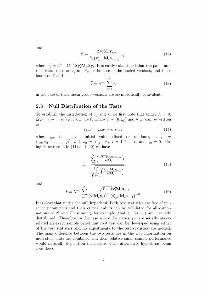
where σ2i = (T − 1)−1∆y′iMe∆yi. It is easily established that the panel unit

root tests based on τφ and τφ in the case of the pooled versions, and thosebased on τ and

τ = N−1

N∑i=1

τi (13)

in the case of their mean group versions are asymptotically equivalent.

2.3 Null Distribution of the Tests

To establish the distribution of τφ and τ , we first note that under φi = 0,∆yi = σivi = σi(vi1, vi2, ..., viT )′, where vi v (0, IT ) and yi,−1 can be writtenas

yi,−1 = yi0eT + σisi,−1, (14)

where yi0 is a given initial value (fixed or random), si,−1 =(si0, si1, . . . , si,T−1)

′ , with sit =∑t

j=1 vij, t = 1, 2, ..., T, and si0 = 0. Us-ing these results in (11) and (12) we have

τφ =

N∑i=1

(√T−1v′iMesi,−1

v′iMevi

)

√N∑

i=1

(s′i,−1Mesi,−1

v′iMevi

) , (15)

and

τ = N−1

N∑i=1

√T − 1v′iMesi,−1

(v′iMevi)1/2 (

s′i,−1Mesi,−1

)1/2. (16)

It is clear that under the null hypothesis both test statistics are free of nui-sance parameters and their critical values can be tabulated for all combi-nations of N and T assuming, for example, that εit (or vit) are normallydistributed. Therefore, in the case where the errors, εit, are serially uncor-related an exact sample panel unit root test can be developed using eitherof the test statistics and no adjustments to the test statistics are needed.The main difference between the two tests lies in the way information onindividual units are combined and their relative small sample performancewould naturally depend on the nature of the alternative hypothesis beingconsidered.

7

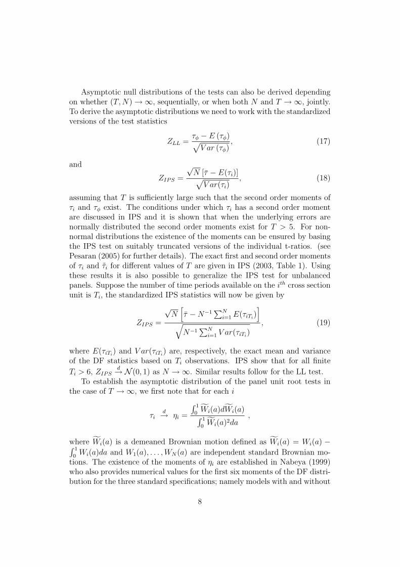
Asymptotic null distributions of the tests can also be derived dependingon whether (T, N) →∞, sequentially, or when both N and T →∞, jointly.To derive the asymptotic distributions we need to work with the standardizedversions of the test statistics

ZLL =τφ − E (τφ)√

V ar (τφ), (17)

and

ZIPS =

√N [τ − E(τi)]√

V ar(τi), (18)

assuming that T is sufficiently large such that the second order moments ofτi and τφ exist. The conditions under which τi has a second order momentare discussed in IPS and it is shown that when the underlying errors arenormally distributed the second order moments exist for T > 5. For non-normal distributions the existence of the moments can be ensured by basingthe IPS test on suitably truncated versions of the individual t-ratios. (seePesaran (2005) for further details). The exact first and second order momentsof τi and τi for different values of T are given in IPS (2003, Table 1). Usingthese results it is also possible to generalize the IPS test for unbalancedpanels. Suppose the number of time periods available on the ith cross sectionunit is Ti, the standardized IPS statistics will now be given by

ZIPS =

√N

[τ −N−1

∑Ni=1 E(τiTi

)]

√N−1

∑Ni=1 V ar(τiTi

), (19)

where E(τiTi) and V ar(τiTi

) are, respectively, the exact mean and varianceof the DF statistics based on Ti observations. IPS show that for all finite

Ti > 6, ZIPSd→ N (0, 1) as N →∞. Similar results follow for the LL test.

To establish the asymptotic distribution of the panel unit root tests inthe case of T →∞, we first note that for each i

τid→ ηi =

∫ 1

0Wi(a)dWi(a)∫ 1

0Wi(a)2da

,

where Wi(a) is a demeaned Brownian motion defined as Wi(a) = Wi(a) −∫ 1

0Wi(a)da and W1(a), . . . , WN(a) are independent standard Brownian mo-

tions. The existence of the moments of ηi are established in Nabeya (1999)who also provides numerical values for the first six moments of the DF distri-bution for the three standard specifications; namely models with and without

8

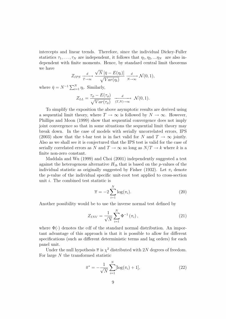
intercepts and linear trends. Therefore, since the individual Dickey-Fullerstatistics τ1, . . . , τN are independent, it follows that η1, η2, ...ηN are also in-dependent with finite moments. Hence, by standard central limit theoremswe have

ZIPSd−−−→

T→∞

√N [η − E(ηi)]√

V ar(ηi)

d−−−→N→∞

N (0, 1),

where η = N−1∑N

i=1 ηi. Similarly,

ZLL =τφ − E(τφ)√

V ar(τφ)

d−−−−−−→(T,N)→∞

N (0, 1).

To simplify the exposition the above asymptotic results are derived usinga sequential limit theory, where T → ∞ is followed by N → ∞. However,Phillips and Moon (1999) show that sequential convergence does not implyjoint convergence so that in some situations the sequential limit theory maybreak down. In the case of models with serially uncorrelated errors, IPS(2003) show that the t-bar test is in fact valid for N and T → ∞ jointly.Also as we shall see it is conjectured that the IPS test is valid for the case ofserially correlated errors as N and T →∞ so long as N/T → k where k is afinite non-zero constant.

Maddala and Wu (1999) and Choi (2001) independently suggested a testagainst the heterogenous alternative H1b that is based on the p-values of theindividual statistic as originally suggested by Fisher (1932). Let πi denotethe p-value of the individual specific unit-root test applied to cross-sectionunit i. The combined test statistic is

π = −2N∑

i=1

log(πi). (20)

Another possibility would be to use the inverse normal test defined by

ZINV =1√N

N∑i=1

Φ−1 (πi) , (21)

where Φ(·) denotes the cdf of the standard normal distribution. An impor-tant advantage of this approach is that it is possible to allow for differentspecifications (such as different deterministic terms and lag orders) for eachpanel unit.

Under the null hypothesis π is χ2 distributed with 2N degrees of freedom.For large N the transformed statistic

π∗ = − 1√N

N∑i=1

[log(πi) + 1], (22)

9

is shown to have a standard normal limiting null distribution as T, N →∞,sequentially.

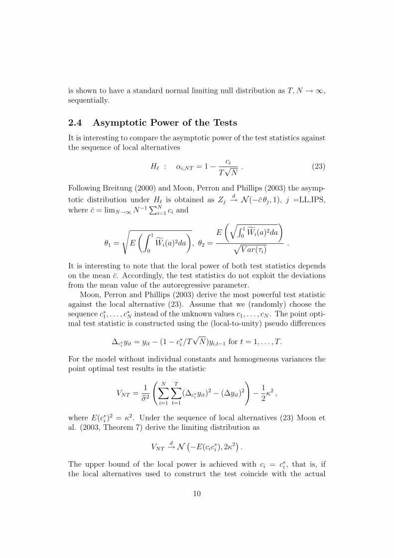
2.4 Asymptotic Power of the Tests

It is interesting to compare the asymptotic power of the test statistics againstthe sequence of local alternatives

H` : αi,NT = 1− ci

T√

N. (23)

Following Breitung (2000) and Moon, Perron and Phillips (2003) the asymp-

totic distribution under H` is obtained as Zjd→ N (−c θj, 1), j =LL,IPS,

where c = limN→∞ N−1∑N

i=1 ci and

θ1 =

√E

(∫ 1

0

Wi(a)2da

), θ2 =

E

(√∫ 1

0Wi(a)2da

)

√V ar(τi)

.

It is interesting to note that the local power of both test statistics dependson the mean c. Accordingly, the test statistics do not exploit the deviationsfrom the mean value of the autoregressive parameter.

Moon, Perron and Phillips (2003) derive the most powerful test statisticagainst the local alternative (23). Assume that we (randomly) choose thesequence c∗1, . . . , c

∗N instead of the unknown values c1, . . . , cN . The point opti-

mal test statistic is constructed using the (local-to-unity) pseudo differences

∆c∗i yit = yit − (1− c∗i /T√

N)yi,t−1 for t = 1, . . . , T.

For the model without individual constants and homogeneous variances thepoint optimal test results in the statistic

VNT =1

σ2

(N∑

i=1

T∑t=1

(∆c∗i yit)2 − (∆yit)

2

)− 1

2κ2 ,

where E(c∗i )2 = κ2. Under the sequence of local alternatives (23) Moon et

al. (2003, Theorem 7) derive the limiting distribution as

VNTd→ N (−E(cic

∗i ), 2κ

2).

The upper bound of the local power is achieved with ci = c∗i , that is, ifthe local alternatives used to construct the test coincide with the actual

10

alternative. Unfortunately, in practice it seems extremely unlikely that onecould select values of c∗i that are perfectly correlated with the true values, ci.If, on the other hand, the variates c∗i are independent of ci, then the poweris smaller than the power of a test using identical values c∗i = c∗ for all i.This suggests that if there is no information about variation of ci, then a testcannot be improved by taking into account a possible heterogeneity of thealternative.

2.5 Heterogeneous Trends

To allow for more general mean functions we consider the model:

yit = δ′idit + yit , (24)

where dit represents the deterministics and ∆yit = φiyi,t−1 + εit. For themodel with a constant mean we let dit = 1 and the model with individualspecific time trends dit is given by dit = (1, t)′. Furthermore, structuralbreaks in the mean function can be accommodated by including (possiblyindividual specific) dummy variables in the vector dit. The parameter vectorδi is assumed to be unknown and has to be estimated. For the Dickey-Fullertest statistic the mean function is estimated under the alternative, that is,for the model with a time trend δ′idit results from a regression of yit on aconstant and t (t = 1, 2, . . . , T ). Alternatively, the mean function can alsobe estimated under the null hypothesis (cf. Schmidt and Phillips, 1992) orunder a local alternative (Elliott et al., 1996).

Including deterministic terms may have an important effect on theasymptotic properties of the test. Let ∆yt and yi,t−1 denote estimates for∆yit = ∆yit−E(∆yit) and yi,t−1 = yi,t−1−E(yi,t−1). In general, running theregression

∆yit = φyi,t−1 + eit

does not render a t-statistic with a standard normal limiting distributiondue to the fact that yi,t−1 is correlated with eit. For example, if dit is an

individual specific constant such that yit = yit − T−1(yi0 + · · · + yi,T−1) weobtain under the null hypothesis

limT→∞

1

TE

T∑

t=1

eityi,t−1

= −σ2

i /2 .

It follows that the t-statistic of φ = 0 tends to −∞ as N or T tends toinfinity.

11

To correct for the bias, Levin et al. (2002) suggested using the correctionterms

aT (δ) = E

(1

σ2i T

T∑t=1

∆yityi,t−1

)(25)

b2T (δ) =

V ar

(T−1

T∑t=1

∆yityi,t−1

)

σ2i E

(T−1

T∑t=1

y2

i,t−1

) (26)

where δ = (δ′1, δ′2, ...., δ

′N)′, and δi is the estimator of the coefficients of the

deterministics, dit, in the OLS regression of yit on dit. The corrected, stan-dardized statitic is given by

ZLL(δ) =

[N∑

i=1

T∑t=1

∆yityi,t−1/σ

2i

]−NTaT (δ)

bT (δ)

√N∑

i=1

T∑t=1

y2

i,t−1/σ2i

.

Levin et al. (2002) present simulated values of aT (δ) and bT (δ) for modelswith constants, time trends and various values of T . A problem is, however,that for unbalanced data sets no correction terms are tabulated.

Alternatively, the test statistic may be corrected such that the adjustedt-statistic

Z∗LL(δ) = [ZLL(δ)− a∗T (δ)]/b∗T (δ)

is asymptotically standard normal. Harris and Tzavalis (1999) derive thesmall sample values of a∗T (δ) and b∗T (δ) for T fixed and N → ∞. Therefore,their test statistic can be applied for small values of T and large values of N .

An alternative approach is to avoid the bias – and hence the correctionterms – by using alternative estimates of the deterministic terms. Breitungand Meyer (1994) suggest using the initial value yi0 as an estimator of theconstant term. As argued by Schmidt and Phillips (1992), the initial value isthe best estimate of the constant given the null hypothesis is true. Using thisapproach the regression equation for a model with a constant term becomes

∆yit = φ∗(yi,t−1 − yi0) + vit .

Under the null hypothesis, the pooled t-statistic of H0 : φ∗ = 0 has a standardnormal limit distribution.

12

For a model with a linear time trend a minimal invariant statistic isobtained by the transformation (cf. Ploberger and Phillips 2002)

x∗it = yit − yi0 − t

T(yiT − yi0) .

In this transformation subtracting yi0 eliminates the constant and (yiT −yi0)/T = (∆yi1 + · · ·+ ∆yiT )/T is an estimate of the slope of the individualtrend function.

To correct for the mean of ∆yit a Helmert transformation can be used

∆y∗it = st

[∆yit − 1

T − t(∆yi,t+1 + · · ·+ ∆yiT )

], t = 1, . . . , T − 1

where s2t = (T − t)/(T − t + 1) (cf. Arellano, 2003, p. 17). Using these

transformations the regression equation becomes

∆y∗it = φ∗x∗i,t−1 + vit . (27)

It is not difficult to verify that under the null hypothesis E(∆y∗itx∗i,t−1) = 0

and, thus, the t-statistic for φ∗ = 0 is asymptotically standard normallydistributed (cf. Breitung, 2000).

The test against heterogeneous alternatives H1b can be easily adjustedfor individual specific deterministic terms such as linear trends or seasonaldummies. This can be done by computing IPS statistics, defined by (18) and(19) for the balanced and unbalanced panels, using Dickey-Fuller t-statisticsbased on DF regressions including the deterministics δ′idit, where dit = 1 inthe case of a constant term, dit = (1, t)′ in the case of models with a lineartime trend and so on. The mean and variance corrections should, however, becomputed to match the nature of the deterministics. Under a general settingIPS (2003) have shown that the ZIPS statistic converges in distribution to astandard normal variate as N, T →∞, jointly.

In a straightforward manner it is possible to include dummy variables inthe vector dit that accommodate structural breaks in the mean function (see,e.g., Murray and Papell, 2002; Tzavalis, 2002; Carrion-I-Sevestre, Del Barrioand Lopez-Bazo, 2004; Breitung and Candelon, 2005; Im, Lee and Tieslau,2005).

2.6 Short-run Dynamics

If it is assumed that the error in the autoregression (1) is a serially correlatedstationary process, the short-run dynamics of the errors can be accounted forby including lagged differences

∆yit = δ′idit + φiyi,t−1 + γi1∆yi,t−1 + · · ·+ γi,pi∆yi,t−pi

+ εit . (28)

13

For example, the IPS statistics (18) and (19) developed for balanced andunbalanced panels can now be constructed using the ADF(pi) statistics basedon the above regressions. As noted in IPS (2003), small sample propertiesof the test can be much improved if the standardization of the IPS statisticis carried out using the simulated means and variances of τi(pi), the t-ratioof φi computed based on ADF(pi) regressions. This is likely to yield betterapproximations, since E [τi(pi)], for example, makes use of the informationcontained in pi while E [τi(0)] = E(τi) does not. Therefore, in the seriallycorrelated case IPS propose the following standardized t-bar statistic

ZIPS =

√N

τ − 1

N

∑Ni=1 E [τi(pi)]

√

1N

∑Ni=1 V ar [τi(pi)]

d−−−−−−→(T,N)→∞

N (0, 1). (29)

The value of E [τi(p)] and V ar [τi(p)] simulated for different values of T andp, are provided in Table 3 of IPS. These simulated moments also allow theIPS panel unit root test to be applied to unbalanced panels with seriallycorrelated errors.

For tests against the homogenous alternatives, φ1 = · · · = φN = φ < 0,Levin et al. (2002) suggest removing all individual specific parameters withina first step regression such that eit (vi,t−1) are the residuals from a regressionof ∆yit (yi,t−1) on ∆yi,t−1, . . . , ∆yi,t−pi

and dit. In the second step the commonparameter φ is estimated from a pooled regression

(eit/σi) = φ(vi,t−1/σi) + νit ,

where σ2i is the estimated variance of eit. Unfortunately, the first step regres-

sions are not sufficient to remove the effect of the short-run dynamics on thenull distribution of the test. Specifically,

limT→∞

E

[1

T − p

T∑t=p+1

eitvi,t−1/σ2i

]=

σi

σi

a∞(δ) ,

where σ2i is the long-run variance and a∞(δ) denotes the limit of the correction

term given in (25). Levin et al. (2002) propose a nonparametric (kernelbased) estimator for σ2

i

s2i =

1

T

[T∑

t=1

∆y2

it + 2K∑

l=1

(K + 1− l

K + 1

) (T∑

t=l+1

∆yit∆yi,t−l

)], (30)

where ∆yit denotes the demeaned difference and K denotes the truncationlag. As noted by Phillips and Ouliaris (1990), in a time series context the

14

estimator of the long-run variance based on differences is inappropriate sinceunder the stationary alternative s2

i

p→ 0 and, thus, using this estimator yieldsan inconsistent test. In contrast, in the case of panels the use of s2

i improves

the power of the test, since with s2i

p→ 0 the correction term drops out andthe test statistic tends to −∞.

It is possible to avoid the use of a kernel based estimator of the long-runvariance by using an alternative approach suggested by Breitung and Das(2005a). Under the null hypothesis we have

γi(L)∆yit = δ′idit + εit ,

where γi(L) = 1 − γi1L − · · · − γi,piLp and L is the lag operator. It fol-

lows that gt = γi(L)[yit − E(yit)] is a random walk with uncorrelated incre-ments. Therefore, the serial correlation can be removed by replacing yit bythe pre-whitened variable yit = γi(L)yit, where γi(L) is an estimator of thelag polynomial obtained from the least-square regression

∆yit = δ′idit + γi1∆yi,t−1 + · · ·+ γi,pi∆yi,t−pi

+ εit . (31)

This approach may also be used for modifying the “unbiased statistic” basedon the t-statistic of φ∗ = 0 in (27). The resulting t-statistic has a standardnormal limiting distribution as T →∞ is followed by N →∞.

Pedroni and Vogelsang (2005) have proposed a test statistic that avoidsthe specification of the short-run dynamics by using an autoregressive approx-imation. Their test statistic is based on the pooled variance ratio statistic

ZwNT =

Tci(0)

Ns2i

,

where ci(`) = T−1∑T

t=`+1yit

yi,t−`, yit = yit − δ′idit and s2i is the untruncated

Bartlett kernel estimator defined as s2i =

∑T+1`=−T+1(1 − |`|/T )ci(`). As has

been shown by Kiefer and Vogelsang (2002) and Breitung (2002), the limitingdistribution of such “nonparametric” statistics does not depend on nuisanceparameters involved by the short run dynamics of the processes. Accordingly,no adjustment for short-run dynamics is necessary.

2.7 Other Approaches to Panel Unit Root Testing

An important problem of combining Dickey-Fuller type statistics in a panelunit root test is that they involve a nonstandard limiting distribution. Ifthe panel unit root statistic is based on a standard normally distributed teststatistic zi, then N−1/2

∑Ni=1 zi has a standard normal limiting distribution

15

even for a finite N . In this case no correction terms need to be tabulated toaccount for the mean and the variance of the test statistic.

Chang (2002) proposes a nonlinear instrumental variable (IV) approach,where the transformed variable

wi,t−1 = yi,t−1e−ci|yi,t−1|

with ci > 0 is used as an instrument for estimating φi in the regression∆yit = φiyi,t−1 + εit (which may also include deterministic terms and laggeddifferences). Since wi,t−1 tends to zero as yi,t−1 tends to ±∞ the trendingbehavior of the nonstationary variable yi,t−1 is eliminated. Using the resultsof Chang, Park and Phillips (2001), Chang (2002) showed that the Waldtest of φ = 0 based on the nonlinear IV estimator possesses a standardnormal limiting distribution. Another important property of the test is thatthe nonlinear transformation also takes account of possible contemporaneousdependence among the cross section units. Accordingly, Chang’s panel unitroot test is also robust against cross-section dependence.

It should be noted that wi,t−1 ∈ [−(cie)−1, (cie)

−1] with a maximum (min-imum) at yi,t−1 = 1/ci (yi,t−1 = −1/ci). Therefore, the choice of the param-eter ci is crucial for the properties of the test. First, the parameter shouldbe proportional to inverse of the standard deviations of ∆yit. Chang notesthat if the time dimension is small, the test slightly over-rejects the nulland therefore she proposes to use a larger value of K to correct for the sizedistortions.

An alternative approach to obtain an asymptotically standard normal teststatistic is to adjust the given samples in all cross-sections so that they allhave sums of squares y2

i1 + · · ·+ y2iki

= σ2i cT

2 + hi, where hip→ 0 as T →∞.

In other words, the panel data set becomes an unbalanced panel with ki

time periods in the i’th unit. Chang calls this setting the “equi-squared sumcontour”, whereas the traditional framework is called the “equi-sample-sizecontour”. The nice feature of this approach is that it yields asymptoticallystandard normal test statistics. An important drawback is, however, thata large number of observations may be discarded by applying this contourwhich may result in a severe loss of power.

Hassler, Demetrescu and Tarcolea (2004) have suggested to use the LMstatistic for a fractional unit root as an asymptotically normally distributedtest statistic. This test statistic is uniformly most powerful against fractionalalternatives of the form (1−L)dyit = εit with d < 1. Although usually panelunit root tests are used to decide whether the series are I(1) or I(0), it can beargued that fractional unit root tests also have a good (albeit not optimal)power against the I(0) alternative (e.g. Robinson, 1994).

16

As in the time series case it is possible to test the null hypothesis that theseries are stationary against the alternative that (at least some of) the seriesare nonstationary. The test suggested by Tanaka (1990) and Kwiatkowski etal. (1992) is designed to test the hypothesis H∗

0 : θi = 0 in the model

yit = δ′idit + θirit + uit , t = 1, . . . , T, (32)

where ∆rit is white noise with unit variance and uit is stationary. The cross-section specific KPSS statistic is

κi =1

T 2σ2T,i

T∑t=1

S2it ,

where σ2T,i denotes a consistent estimator of the long-run variance of ∆yit and

Sit =∑t

`=1

(yi` − δ′idi`

)is the partial sum of the residuals from a regression

of yit on the deterministic terms (a constant or a linear time trend). Theindividual test statistics can be combined as in the test suggested by IPS(2003) yielding

κ = N−1/2

∑Ni=1 [κi − E(κi)]√

V ar(κi),

where asymptotic values of E(κi) and V ar(κi) are derived in Hadri (2000)and values for finite T and N → ∞ are presented in Hadri and Larsson(2005).

The test of Harris, Leybourne and McCabe (2004) is based on the sta-tionarity statistic

Zi(k) =√

T ci(k)/ωzi(k),

where ci(k) denotes the usual estimator of the covariance at lag k of crosssection unit i and ω2

zi(k) is an estimator of the long-run variance of zkit =

(yit − δ′idit)(yi,t−k − δ′idi,t−k). The intuition behind this test statistic is thatfor a stationary and ergodic time series we have E[ci(k)] → 0 as k → ∞.Since ω2

zi is a consistent estimator for the variance of ci(k) it follows that Zi(k)converges to a standard normally distributed random variable as k →∞ andk/√

T → δ < ∞.

3 Second Generation Panel Unit Root Tests

3.1 Cross Section Dependence

So far we have assumed that the time series yitTt=0 are independent across i.

However, in many macroeconomic applications using country or regional data

17

it is found that the time series are contemporaneously correlated. Prominentexamples are the analysis of purchasing power parity and output conver-gence.4 The literature on modelling of cross section dependence in largepanels is still developing and in what follows we provide an overview of someof the recent contributions.5

Cross section dependence can arise due to a variety of factors, such asomitted observed common factors, spatial spill over effects, unobserved com-mon factors, or general residual interdependence that could remain even whenall the observed and unobserved common effects are taken into account. Ab-stracting from common observed effects and residual serial correlation a gen-eral specification for cross sectional error dependence can be written as

∆yit = −µiφi + φiyi,t−1 + uit,

whereuit = γ′ift + ξit, (33)

orut = Γf t + ξt, (34)

ut = (u1t, u2t, ..., uNt)′, ft is an m × 1 vector of serially uncorrelated un-

observed common factors, and ξt = (ξ1t, ξ2t, ..., ξNt)′ is an N × 1 vector of

serially uncorrelated errors with mean zero and the positive definite covari-ance matrix Ωξ, and Γ is an N × m matrix of factor loadings defined byΓ = (γ1, γ2, ..., γN)′. 6 Without loss of generality the covariance matrix of ftis set to Im, and it is assumed that ft and ξt are independently distributed.If γ1 = · · · = γN , then θt = γ′ft is a conventional “time effect” that can beremoved by subtracting the cross section means from the data. In generalit is assumed that γi, the factor loading for the ith cross section unit, differsacross i and represents draws from a given distribution.

Under the above assumptions and conditional on γi, i = 1, 2, ..., N , thecovariance matrix of the composite errors, ut, is given by Ω = ΓΓ′ + Ωξ.It is clear that without further restrictions the matrices Γ and Ωξ are notseparately identified. The properties of Ω also crucially depend on the rela-tive eigenvalues of ΓΓ′ and Ωξ, and their limits as N →∞. Accordingly twocases of cross-section dependence can be distinguished: (i) Weak dependence.In this case it is assumed that the eigenvalues of Ω are bounded as N →∞.

4See, for example, O’Connell (1998) and Phillips and Sul (2003b). Tests for crosssection independence of errors with applications to output growth equations are consideredin Pesaran (2004a).

5A survey of the second generation panel unit root tests is also provided by Hurlin andMignon (2004).

6The case where ft and/or ξit might be serially correlated will be considered below.

18

This assumption rules out the presence of unobserved common factors, butallows the cross section units to be, for example, spatially correlated witha finite number of “neighbors”. (ii) Strong dependence. In this case someeigenvalues of Ω are O(N), which arises when there are unobserved commonfactors. When N is fixed as T → ∞ both sources of dependence could bepresent. But for N → ∞ (and particularly when N > T ) it seems onlysensible to consider cases where rank(Γ) = m ≥ 1 and Ωξ is a diagonalmatrix.

A simple example of panel data models with weak cross section depen-dence is given by

∆y1t

...∆yNt

=

a1...

aN

+ φ

y1,t−1...

yN,t−1

+

u1t...

uNt

(35)

or∆yt = a + φyt−1 + ut, (36)

where ai = −φµi and ∆yt, yt−1, a and ut are N×1 vectors. The cross-sectioncorrelation is represented by a non-diagonal matrix

Ω = E(utu′t), for all t,

with bounded eigenvalues. For the model without constants Breitung andDas (2005a) showed that the regression t-statistic of φ = 0 in (36) is asymp-totically distributed as N (0, vΩ) where

vΩ = limN→∞

tr(Ω2/N)

(trΩ/N)2. (37)

Note that tr(Ω) and tr(Ω2) are O(N) and, thus, vΩ converges to a constantthat can be shown to be larger than one. This explains why the test ignoringthe cross-correlation of the errors has a positive size bias.

3.2 Tests Based on GLS regressions

Since (36) can be seen as a seemingly unrelated regression system, O’Connell(1998) suggests to estimate the system by using a GLS estimator (see also

Flores, et al., 1999). Let Ω = T−1∑T

t=1 utu′t denote the sample covariance

matrix of the residual vector. The GLS t-statistic is given by

tgls(N) =

T∑t=1

∆y′tΩ−1yt−1

√T∑

t=1

y′t−1Ω−1yt−1

,

19

where yt is the vector of demeaned variables. Harvey and Bates (2003) derivethe limiting distribution of tgls(N) for a fixed N and as T →∞, and tabulateits asymptotic distribution for various values of N . Breitung and Das (2005a)show that if yt = yt − y0 is used to demean the variables and T → ∞ isfollowed by N → ∞, then the GLS t-statistic possesses a standard normallimiting distribution.

The GLS approach cannot be used if T < N as in this case the estimatedcovariance matrix Ω is singular. Furthermore, Monte Carlo simulations sug-gest that for reasonable size properties of the GLS test, T must be substan-tially larger than N (e.g. Breitung and Das, 2005a). Maddala and Wu (1999)and Chang (2004) have suggested a bootstrap procedure that improves thesize properties of the GLS test.

3.3 Test statistics based on OLS regressions

An alternative approach based on “panel corrected standard errors” (PCSE)is considered by Jonsson (2005) and Breitung and Das (2005a). In the model

with weak dependence, the variance of the OLS estimator φ is consistentlyestimated by

var(φ) =

T∑t=1

y′t−1Ωyt−1

(T∑

t=1

y′t−1yt−1

)2 .

If T → ∞ is followed by N → ∞ the robust t statistic trob = φ/

√var(φ) is

asymptotically standard normally distributed (Breitung and Das, 2005a).If it is assumed that the cross correlation is due to common factors, then

the largest eigenvalue of the error covariance matrix, Ω, is Op(N) and therobust PCSE approach breaks down. Specifically, Breitung and Das (2005b)showed that in this case trob is distributed as the ordinary Dickey-Fuller testapplied to the first principal component.

In the case of a single unobserved common factor, Pesaran (2005) hassuggested a simple modification of the usual test procedure. Let yt =N−1

∑Ni=1 yit and ∆yt = N−1

∑Ni=1 ∆yit = yt − yt−1. The cross section aug-

mented Dickey-Fuller (CADF) test is based on the following regression

∆yit = ai + φiyi,t−1 + biyt−1 + ci∆yt + eit .

In this regression the additional variables ∆yt and yt−1 are√

N -consistentestimators for the rescaled factors γft and γ

∑t−1j=0 fj, where γ = N−1

∑Ni=1 γi.

Pesaran (2005) showed that the distribution of the regression t-statistic for

20

φi = 0 is free of nuisance parameters. To test the unit root hypothesis ina heterogenous panel the average of the N individual CADF t-statistics (orsuitably truncated version of them) can be used. Coakley et al. (2005) applythe CADF test to real exchange rates of 15 OECD countries.

3.4 Other Approaches

A similar approach was proposed by Moon and Perron (2004) and Phillipsand Sul (2003a). The test of Moon and Perron (2004) is based on a prin-cipal components estimator of m < N common factors f1t, . . . , fmt in (33).The number of common factors can be consistently determined by using theinformation criteria suggested by Bai and Ng (2002). Let Vm = [v1, . . . , vm]denote the matrix of m orthonormal eigenvectors associated with m largesteigenvalues of Ω. The vector of common factors are estimated as

ft = [f1t, . . . , fmt]′ = V′

m∆yt .

As shown by Bai and Ng (2002), the principal component estimator ft yieldsa consistent estimator of the factor space as min(N, T ) → ∞. Thus, theelements of the vector

(IN − VmV′

m

)∆yt ≡ QbVm

∆yt, (38)

are consistent estimates of the idiosyncratic components ξit as N → ∞.Therefore, by assuming that ξit is i.i.d., the pooled regression t-statistic

t∗MP =

T∑t=1

∆y′tQbVmyt−1

√T∑

t=1

y′t−1QbVmyt−1

.

has a standard normal limiting distribution as (N, T →∞) and lim infN,T→∞log N/ log T → 0 (cf. Moon and Perron 2004).

4 Cross-unit cointegration

As argued by Banerjee, Marcellino and Osbat (2005) panel unit root testsmay be severely biased if the panel units are cross-cointegrated, namely ifunder the null hypothesis (of unit roots) one or more linear combinationsof yt are stationary. This needs to be distinguished from the case wherethe errors are cross correlated without necessarily involving cointegration

21

across the cross section units. Under the former two or more cross sectionunits must share at least one common stochastic trend. Such a situation islikely to occur if the PPP hypothesis is examined (cf. Lyhagen, 2000 andBanerjee et al. 2005). The tests proposed by Moon and Perron (2004) andPesaran (2005) are not appropriate if yt contains common stochastic trendsand their use could lead to misleading conclusions. For example, in thepresence of cross-section cointegration the common trends are identified ascommon factors and by performing the transformation (38) these commonfactors are removed from the data. If the remaining idiosyncratic componentis stationary, the test tends to indicate that the time series are stationary,although all panel units are nonstationary.

To overcome this difficulty Bai and Ng (2004a) have suggested a generalapproach for analyzing the common factors and idiosyncratic componentsseparately. Whereas the tests of Moon and Perron (2004) and Pesaran (2005)assume that only the idiosyncractic components have unit roots, the testprocedure of Bai and Ng (2004a) allows for the possibility of unit roots inidiosyncratic and/or the common stochastic components and attempts toascertain the unit root properties of both components from the data. Forexample, if the idiosyncratic processes are independent random walks, therewill be no cointegration among the panel units. Nevertheless it is possible todetermine the number of common trends and to estimate them consistently asN and T tends to infinity (see also Bai 2004). However, testing for unit rootsin the common components are likely to require particularly large panels;with the power of the test only favourably affected when T is increased.

The common factors are estimated by principal components and coin-tegration tests are used to determine the number of common trends. Fur-thermore, panel unit root tests are applied to the idiosyncratic components.The null hypothesis that the time series have a unit root is rejected if eitherthe test of the common factors or the test for the idiosyncratic componentcannot reject the null hypothesis of nonstationary components. A similartest procedure based on KPSS test statistics are proposed by Bai and Ng(2004b).7

To allow for short-run and long-run (cross-cointegration) dependencies,Chang and Song (2005) suggest a nonlinear instrument variable test proce-dure. As the nonlinear instruments suggested by Chang (2002) are invalidin the case of cross-cointegration panel specific instruments based on the

7An alternative factor extraction method is suggested by Kapetanios (2005) who alsoprovides detailed Monte Carlo results on the small sample performance of panel unit roottests based on a number of alternative estimates of the unobserved common factors. Heshows that the factor-based panel unit root tests tend to perform rather poorly when theunobserved common factor is serially correlated.

22

Hermit function of different order are used as nonlinear instruments. Changand Song (2005) showed that the t-statistic computed from the nonlinear IVstatistic are asymptotically standard normally distributed and, therefore, apanel unit statistics against the heterogeneous alternative H1b can be con-structed that has an standard normal limiting distribution.

Choi and Chue (2004) employ a subsampling procedure to obtain teststhat are robust against a wide range of cross-section dependence such asweak and strong correlation as well as cross-cointegration. To this end thesample is grouped into a number of overlapping blocks of b time periods.Using all (T − b+1) possible overlapping blocks, the critical value of the testis estimated by the respective quantile of the empirical distribution of the(T − b + 1) test statistics computed. The advantage of this approach is thatthe null distribution of the test statistic may depend on unknown nuisanceparameters. Whenever the test statistics converge in distribution to somelimiting null distribution as T → ∞ and N fixed, the subsample criticalvalues converge in probability to the true critical values. Using Monte Carlosimulations Choi and Chue (2004) demonstrate that the size of the subsampletest is indeed very robust against various forms of cross-section dependence.

5 Finite Sample Properties of Panel Unit

Root Tests

It has become standard to distinguish first generation panel unit root teststhat are based on the assumption of independent cross section units andsecond generation tests that allow for some kind of cross-section dependence.Maddala and Wu (1999) compared several first generation tests. For theheterogeneous alternative under consideration they found that in most casesthe Fisher test (20) performs similar or slightly better than the IPS statisticwith respect to size and power. The Levin and Lin statistic (in the versionof the 1993 paper) performs substantially worse. Similar results are obtainedby Choi (2001). Madsen (2003) derived the local power function againsthomogeneous alternatives under different detrending procedures. Her MonteCarlo simulations support her theoretical findings that the test based onestimating the mean under the null hypothesis (i.e. the initial observationis subtracted from the time series) outperforms tests based on alternativedemeaning procedures. Similar findings are obtained by Bond et al. (2002).

Moon and Perron (2004) compare the finite sample powers of alterna-tive tests against the homogeneous alternative. They found that the point-optimal test of Moon et al. (2003) performs best and show that the power

23

of this test is close to the power envelope. Another important finding fromthese simulation studies is the observation that the power of the test dropsdramatically if a time trend is included. This confirms theoretical results onthe local power of panel unit root tests derived by Breitung (2000), Plobergerand Phillips (2002) and Moon, Perron and Phillips (2003).

Hlouskova and Wagner (2005) compare a large number of first generationpanel unit root tests applied to processes with MA(1) errors. Not surpris-ingly, all tests are severely biased as the root of the MA process approachesunity. Overall, the tests of Levin et al. (2002) and Breitung (2000) havethe smallest size distortions. These tests also perform best against the ho-mogenous alternative, where the autoregressive coefficient is the same for allpanel units. Of course this is not surprising as these tests are optimal underhomogeneous alternatives. Furthermore, it turns out that the stationaritytests of Hadri (2000) perform very poorly in small samples. This may be dueto the fact that asymptotic values for the mean and variances of the KPSSstatistics are used, whereas Levin et al. (2002) and IPS (2003) provide valuesfor small T as well.

The relative performance of several second generation tests have beenstudied by Gutierrez (2005), and Gengenbach, Palm and Urbain (2004),where the cross-section dependence is assumed to follow a factor structure.The results very much depend on the underlying model. The simulationscarried out by Gengenbach, Palm and Urbain (2004) show that in general,the mean CADF test has better size properties than the test of Moon andPerron (2004), which tends to be conservative in small samples. Howeverthe latter test appears to have more power against stationary idiosyncraticcomponents. Since these tests remove the common factors, they will even-tually indicate stationary time series in cases where the series are actuallynonstationary due to a common stochastic trend. The results of Gengenbachet al. (2004) also suggest that the approach of Bai and Ng (2004a) is able tocope with this possibility although the power of the unit test applied to thenonstationary component is not very high.

In general, the application of factor models in the case of weak correla-tion does not yield valid test procedures. Alternative unit root tests thatallow for weak cross section dependence are considered in Breitung and Das(2005a). They found that the GLS t-statistic may have a severe size bias if Tis only slightly larger than N . In these cases Chang’s (2004) bootstrap pro-cedure is able to improve the size properties substantially. The robust OLSt-statistic performs slightly worse but outperforms the nonlinear IV test ofChang (2002). However, Monte Carlo simulations recently carried out byBaltagi, Bresson and Pirotte (2005) show that there can be considerable sizedistortions even in panel unit root tests that allow for weak dependence.

24

Interestingly enough Pesaran’s test, which is not designed for weak crosssection dependence, tends to be the most robust to spatial type dependence.

6 Panel Cointegration: General Considera-

tions

The estimation of long-run relationships has been the focus of extensive re-search in time series econometrics. In the case of variables on a single crosssection unit the existence and the nature of long-run relations are investigatedusing cointegration techniques developed by Engle and Granger (1987), Jo-hansen (1991,1995) and Phillips (1991). In this literature residual-based andsystem approaches to cointegration are advanced. In this section we reviewthe panel counter part of this literature. But before considering the problemof cointegration in a panel a brief overview of the cointegration literaturewould be helpful.

Consider the ni time series variables zit = (zi1t, zi2t, . . . , zinit)′ observed

on the ith cross section unit over the period t = 1, 2, ..., T , and suppose thatfor each i

zijt ∼ I(1), j = 1, 2, . . . ., ni.

Then zit is said to form one or more cointegrating relations if there are linearcombinations of zijt’s for j = 1, 2, ..., ni that are I (0) i.e. if there exists anni × ri matrix (ri ≥ 1) such that

β′iri × ni

zit

ni × 1= ξit

ri × 1∼ I (0) .

ri denotes the number of cointegrating (or long-run) relations. The residual-based tests are appropriate when ri = 1, and zit can be partitioned such thatzit = (yit,x

′it)′ with no cointegration amongst the ki×1 (ki = ni−1) variables,

xit. The system cointegration approaches are much more generally applica-ble and allow for ri > 1 and do not require any particular partitioning ofthe variables in zit.

8 Another main difference between the two approaches isthe way the stationary component of ξit is treated in the analysis. Most ofthe residual-based techniques employ non-parametric (spectral density) pro-cedures to model the residual serial correlation in the error correction terms,ξit, whilst vector autoregressions (VAR) are utilized in the development ofsystem approaches.

8System approaches to cointegration analysis that allow for weakly exogenous (or long-run forcing) variables has been considered in Pesaran, Shin and Smith (2000).

25

In panel data models the analysis of cointegration is further complicatedby heterogeneity, unbalanced panels, cross section dependence, cross unitcointegration and the N and T asymptotics. But in cases where ni and Nare small such that ΣN

i=1ni is less than 10, and T is relatively large (T > 100),as noted by Banerjee, Marcellino and Osbat (2004), many of these problemscan be avoided by applying the system cointegration techniques to the pooledvector, zt = (z′1t, z

′2t, ..., z

′Nt)

′. In this setting cointegration will be defined bythe relationships β′zt that could contain cointegration between variables fromdifferent cross section units as well as cointegration amongst the differentvariables specific to a particular cross section unit. This framework can alsodeal with residual cross section dependence since it allows for a general errorcovariance matrix that covers all the variables in the panel.

Despite its attractive theoretical features, the ‘full’ system approach topanel cointegration is not feasible even in the case of panels with moderatevalues of N and ni. See Section 10 below for further details. In practice,cross section cointegration can be accommodated using common factors as inthe work of Bai and Ng (2004), Pesaran (2004b), Pesaran, Schuermann andWeiner (2004, PSW) and its subsequent developments in Dees, di Mauro,Pesaran and Smith (2005, DdPS). Bai and Ng (2004a) consider the simplecase where ni = 1 but allow N and T to be large. But their set up canbe readily generalized so that cointegration within each cross section unit aswell as across the units can be considered. Following DdPS suppose that9

zit = Γiddt + Γif ft + ξit, (39)

for i = 1, ..., N ; t = 1, 2, ..., T , and to simplify the exposition assume thatni = n, where as before dt is the s × 1 vector of deterministics (1, t) orobserved common factors such as oil prices, ft is a m × 1 vector of unob-served common factors, Γid and Γif are n× s and n×m associated unknowncoefficient matrices, ξit is an n× 1 vector of error terms.

Unit root and cointegration properties of zit, i = 1, 2, ..., N , can be ana-lyzed by allowing the common factors, ft, and/or the country-specific factors,ξit, to have unit roots. To see this suppose

∆ft = Λ (L) ηt, ηt ∼ IID (0, Im) , (40)

∆ξit = Ψi (L)vit, vit ∼ IID (0, In) , (41)

9DdPS also allow for common observed macro factors (such as oil prices), but they arenot included to simplify the exposition.

26

where L is the lag operator and

Λ (L) =∞∑

`=0

Λ`m×m

L`, Ψi (L) =∞∑

`=0

Ψi`n×n

L`. (42)

The coefficient matrices, Λ` and Ψi`, i = 1, 2, ..., N , are absolute summable,so that V ar (∆ft) and V ar (∆ξit) are bounded and positive definite, and[Ψi (L)]−1 exists. In particular we require that

||∞∑

`=0

Ψi`Ψ′i`|| ≤ K < ∞, (43)

where K is a fixed constant.Using the familiar decomposition

Λ (L) = Λ (1) + (1− L)Λ∗ (L) , and Ψi (L) = Ψi (1) + (1− L)Ψ∗i (L) ,

the common stochastic trend representations of (40) and (41) can now bewritten as

ft = f0 + Λ (1) st + Λ∗ (L) (ηt − η0) ,

andξit = ξi0 + Ψi (1) sit + Ψ∗

i (L) (vit − vi0) ,

where

st =t∑

j=1

ηj and sit =t∑

j=1

vij.

Using the above results in (39) now yields

zit = ai + Γiddt + ΓifΛ (1) st + Ψi (1) sit

+ΓifΛ∗ (L) ηt + Ψ∗

i (L)vit,

where10

ai = Γif [f0 −Λ∗ (L) η0] + ξi0 −Ψ∗i (L)vi0.

In this representation Λ (1) st and Ψi (1) sit can be viewed as common globaland individual-specific stochastic trends, respectively; whilst Λ∗ (L) ηt andΨ∗

i (L)vit are the common and individual-specific stationary components.From this result it is clear that, in general, it will not be possible to simul-taneously eliminate the two types of the common stochastic trends (globaland individual-specific) in zit.

10In usual case where dt is specified to include an intercept, 1, ai can be absorbed intothe deterministics.

27

Specific cases of interest where it would be possible for zit to form a coin-tegrating vector are when Λ (1) = 0 or Ψi (1) = 0. Under the former panelcointegration exists if Ψi (1) is rank deficient. The number of cointegratingrelations could differ across i and is given by ri = n−Rank [Ψi (1)]. Note thateven in this case zit can be cross-sectionally correlated through the commonstationary components, Λ∗ (L) ηt. Under Ψi (1) = 0 for all i with Λ (1) 6= 0,we will have panel cointegration if there exists n × ri matrices βi such thatβ′iΓifΛ (1) = 0. Notice that this does not require Λ (1) to be rank deficient.

Turning to the case where Λ (1) and Ψi (1) are both non-zero, panelcointegration could still exist but must involve both zit and ft. But since ftis unobserved it must be replaced by a suitable estimate. The global VAR(GVAR) approach of Pesaran et al. (2004) and Dees et al. (2005) implementsthis idea by replacing ft with the (weighted) cross section averages of zit. Tosee how this can be justified first differencing (39) and using (41) note that

[Ψi (L)]−1 (1− L) (zit − Γiddt − Γif ft) = vit.

Using the approximation

(1− L) [Ψi (L)]−1 ≈p∑

`=0

Φi`L` = Φi (L, p) ,

we obtain the following approximate VAR(p) model

Φi (L, p) (zit − Γiddt − Γif ft) ≈ vit. (44)

When the common factors, ft, are observed the model for the ith cross-sectionunit decouples from the rest of the units and can be estimated using theeconometric techniques developed in Pesaran, Shin and Smith (2000) with fttreated as weakly exogenous. But in general where the common factors areunobserved appropriate proxies for the common factors can be used. Thereare two possible approaches, one could either use the principal componentsof the observables, zit, or alternatively following Pesaran (2004b) ft can beapproximated in terms of zt = N−1ΣN

i=1zit, the cross section averages ofthe observables. To see how this procedure could be justified in the presentcontext, average the individual equations given by (39) over i to obtain

zt = Γddt + Γf ft + ξt, (45)

where Γd = N−1ΣNi=1Γid, Γf = N−1ΣN

i=1Γif , and ξt = N−1ΣNi=1ξit. Also, note

from (41) that

ξt − ξt−1 = N−1

N∑j=1

Ψj (L)vjt. (46)

28

But using results in Pesaran (2004b), for each t and as N → ∞ we have

ξt − ξt−1q.m.→ 0, and hence ξt

q.m.→ ξ, where ξ is a time-invariant randomvariable. Using this result in (45) and assuming that the n × m averagefactor loading coefficient matrix, Γf , has full column rank (with n ≥ m) weobtain

ftq.m.→

(Γ′f Γf

)−1

Γf

(zt − Γddt − ξ

),

which justifies using the observable vector dt, zt as proxies for the unob-served common factors.

The various contributions to the panel cointegration literature will nowbe reviewed in the context of the above general set up. First generationliterature on panel cointegration tends to ignore the possible effects of globalunobserved common factors, or attempts to account for them either by cross-section de-meaning or by using observable common effects such as oil pricesor U.S. output. This literature also focusses on residual based approacheswhere it is often assumed that there exists at most one cointegrating relationin the individual specific models. Notable contributions to this strand of theliterature include Kao (1999), Pedroni (1999, 2001, 2004), and more recentlyWesterlund (2005a). System approaches to panel cointegration that allow formore than one cointegrating relations include the work of Larsson, Lyhagenand Lothgren (2001), Groen and Kleibergen (2003) and Breitung (2005) whogeneralized the likelihood approach introduced in Pesaran, Shin and Smith(1999). Like the second generation panel unit root tests, recent contributionsto the analysis of panel cointegration have also emphasized the importance ofallowing for cross section dependence which, as we have noted above, couldbe due to the presence of common stationary or non-stationary componentsor both. The importance of allowing for the latter has been emphasizedin Banerjee, Marcellino and Osbat (2004) through the use of Monte Carloexperiments in the case of panels where N is very small, at most 8 in theiranalysis. But to date a general approach that is capable of addressing all thevarious issues involved does not exist if N is relatively large.

We now consider in some further detail the main contributions, beginningwith a brief discussion of the spurious regression problem in panels.

7 Residual-Based Approaches to Panel Coin-

tegration

Under this approach zit is partitioned as zit = (yit,x′it)′ and the following

regressionsyit = δ′idit + x′itβ + uit, i = 1, 2, ..., N, (47)

29

are considered, where as before δ′idit represent the deterministics and the k×1vector of regressors, xit, are assumed to be I(1) and not cointegrated. How-ever, the innovations in ∆xit, denoted by εit = ∆xit − E(∆xit), are allowedto be correlated with uit. Residual-based approaches to panel cointegrationfocus on testing for unit roots in OLS or panel estimates of uit.

7.1 Spurious regression

Let wit = (uit, ε′it)′ and assume that the conditions for the functional central

limit theorem are satisfied such that

1√T

[·T ]∑t=1

witd→ Σ

1/2i Wi(·),

where Wi is a (k + 1)× 1 vector of standard Brownian motions,d→ denotes

weak convergence on D[0, 1] and

Σi =

[σ2

i,u σi,uε

σ′i,uε Σi,εε

].

Kao (1999) showed that in the homogeneous case with Σi = Σ, i = 1, . . . , N ,

and abstracting from the deterministics, the OLS estimator β converges inprobability to the limit Σ−1

εε σεu, where it is assumed that wit is i.i.d. acrossi. In the heterogeneous case Σεε and σεu are replaced by the means Σεε =N−1

∑Ni=1 Σi,εε and σεu = N−1

∑Ni=1 σi,εu, respectively (cf. Pedroni 2000).

In contrast, the OLS estimator of β fails to converge within a pure timeseries framework (cf. Phillips 1987). On the other hand, if xit and yit areindependent random walks, then the t-statistics for the hypothesis that onecomponent of β is zero is Op(T

1/2) and, therefore, the t-statistic has similarproperties as in the time series case. As demonstrated by Entorf (1997) andKao (1999), the tendency for spuriously indicating a relationship among yit

and xit may even be stronger in panel data regressions as in the pure timeseries case. Therefore, it is important to test whether the errors in a paneldata regression like (47) are stationary.

7.2 Tests of Panel Cointegration

As in the pure time series framework, the variables in a regression functioncan be tested against cointegration by applying unit roots tests of the sortsuggested in the previous sections to the residuals of the estimated regression.Unfortunately, panel unit root tests cannot be applied to the residuals in

30

(47) if xit is (long-run) endogenous, that is, if σεu 6= 0. Letting T → ∞ befollowed by N → ∞, Kao (1999) show that the limiting distribution of theDF t-statistic applied to the residuals of a pooled OLS regression of (47) is

(tφ −√

N µK)/σKd→ N (0, 1), (48)

where the values of µK and σK depend on the kind of deterministics includedin the regression, the contemporaneous covariance matrix E(witw

′it) and the

long-run covariance matrix Σi. Kao (1999) proposed adjusting tφ by usingconsistent estimates of µK and σK , where he assumes that the nuisance pa-rameters are the same for all panel units (homogenous short-run dynamics).

Pedroni (2004) suggest two different test statistics for the models with

heterogeneous cointegration vectors. Let uit = yit − δ′idit − β′ixit denote theOLS residual of the cointegration regression. Pedroni considers two differentclasses of test statistics: (i) the “panel statistic” that is equivalent to the unitroot statistic against homogeneous alternatives and (ii) the “Group Meanstatistic” that is analogous to the panel unit root tests against heterogeneousalternatives. The two versions of the t statistic are defined as

panel ZPt =

(σ2

NT

N∑i=1

T∑t=1

u2i,t−1

)−1/2 (N∑

i=1

T∑t=1

ui,t−1uit − T

N∑i=1

λi

)

group-mean ZPt =N∑

i=1

(σ2

ie

T∑t=1

u2i,t−1

)−1/2 (T∑

t=1

ui,t−1uit − T λi

)

where λi is a consistent estimator of the one-sided long run variance λi =∑∞j=1 E(eitei,t−j), eit = uit − δiui,t−1, δi = E(uitui,t−1)/E(u2

i,t−1), σ2ie denotes

the estimated variance of eit and σ2NT = N−1

∑Ni=1 σ2

ie. Pedroni presents

values of µp, σ2p and µp, σ

2p such that (ZPt−µp

√N)/σp and (ZPt− µp

√N)/σp

have standard normal limiting distributions under the null hypothesis.Other residual-based panel cointegration tests include the recent contri-

bution of Westerlund (2005a) that are based on variance ratio statistics anddo not require corrections for the residual serial correlations.

The finite sample properties of some residual based test for panel cointe-gration are discussed in Baltagi and Kao (2000). Gutierrez (2003) comparesthe power of various panel cointegration test statistics. He shows that inhomogeneous panels with a small number of time periods Kao’s tests tend tohave higher power than Pedroni’s tests, whereas in panels with large T thelatter tests performs best. Both test outperform the system test suggestedby Larssen et al. (2001).

31

8 Tests for Multiple Cointegration

It is also possible to adapt Johansen’s (1995) multivariate test based ona VAR representation of the variables. Let Λi(r) denote the cross-sectionspecific likelihood-ratio (“trace”) statistic of the hypothesis that there are(at most) r stationary linear combinations in the cointegrated VAR systemgiven by zit = (yit,x

′it)′. Following the unit root test proposed in IPS (2003),

Larsson et al. (2001) suggested the standardized LR-bar statistic

Λ(r) =1√N

N∑i=1

Λi(r)− E[λi(r)]√V ar[λi(r)]

,

to test the null hypothesis that r = 0 against the alternative that at mostr = r0 ≥ 1. Using a sequential limit theory it can be shown that Λ(r) isasymptotically standard normally distributed. Asymptotic values of E[λi(r)]and V ar[λi(r)] are tabulated in Larsson et al. (2001) for the model withoutdeterministic terms and Breitung (2005) for models with a constant and alinear time trend. Unlike the residual-based tests, the LR-bar test allows forthe possibility of multiple cointegration relations in the panel.

It is also possible to test the null hypothesis that the errors of the coin-tegration regression are stationary. That is, under the null hypothesis itis assumed that yit,xit are cointegrated with cointegration rank r = 1. Mc-Coskey and Kao (1998) suggest a panel version of Shin’s (1994) cointegrationtest based on the residuals of a fully modified OLS regression. Westerlund(2005b) suggests a related test procedure based on the CUSUM statistic.

9 Estimation of Cointegrating Relations in

Panels

9.1 Single Equation Estimators

First, we consider a single-equation framework where it is assumed that yit

and the k× 1 vector of regressors xit are I(1) with at most one cointegratingrelations amongst them, namely that there exists a linear relationship of theform (47) such that the error uit is stationary. As before it is assumed thatzit = (yit,x

′it)′ is i.i.d. across i, and the regressors, xit, are not cointegrated.

We do not explicitly consider deterministic terms like individual specific con-stants or trends as the asymptotic theory applies to mean- or trend-adjustedvariables as well.

It is assumed that the vector of coefficients, β, is the same for all cross-section units, that is, a homogeneous cointegration relationship is assumed.

32

Alternatively, it may be assumed that the cointegration parameters are crosssection specific (heterogenous cointegration).

By applying a sequential limit theory it can be shown that the OLS es-timator of β is T

√N consistent and, therefore, the time series dimension

is more informative on the long-run coefficients than the cross-section di-mension. Furthermore, is important to notice that – as in the time seriesframework – the OLS estimator is consistent but inefficient in the modelwith endogenous regressors.

Pedroni (1995) and Phillips and Moon (1999, p. 1085) proposed a “fully-modified OLS” (FM-OLS) approach to obtain an asymptotically efficientestimator for homogenous cointegration vectors. This estimator adjusts forthe effects of endogenous regressors and short-run dynamics of the errors (cf.Phillips and Hansen 1990). To correct for the effect of (long-run) endogeneityof the regressors, the dependent variable is adjusted for the part of the errorthat is correlated with the regressor

y+it = yit − σ′i,εuΣ

−1i,εε∆xit. (49)

A second correction is necessary when computing the OLS estimator

βFM =

[N∑

i=1

T∑t=1

xitx′it

]−1 [N∑

i=1

T∑t=1

(xity+it − λi,εu)

], (50)

where

λi,εu = E

( ∞∑j=0

εi,t−juit

).

The nuisance parameters can be estimated consistently using familiar non-parametric procedures.

An alternative approach is the “Dynamic OLS” (DOLS) estimator sug-gested by Saikkonen (1991). This estimator is based on the error decompo-sition

uit =∞∑

k=−∞γ′k∆xi,t+k + vit , (51)

where vit is orthogonal to all leads and lags of ∆xit. Inserting (51) in theregression (47) yields

yit = β′xit +∞∑

k=−∞γ′k∆xi,t+k + vit . (52)

In practice the infinite sums are truncated at some small numbers of leads andlags (cf. Kao and Chiang 2000, Mark and Sul 2003). Westerlund (2005c)

33

considers data dependent choices of the truncation lags. Kao and Chiang(2000) show that in the homogeneous case with Σi = Σ and individual

specific intercepts the limiting distribution of the DOLS estimator βDOLS isgiven by

T√

N(βDOLS − β)d→ N (0, 6 σ2

u|εΣ−1εε ),

whereσ2

u|ε = σ2u − σ′εuΣ

−1εε σεu.

Furthermore, the FM-OLS estimator possesses the same asymptotic distri-bution as the DOLS estimator. In the heterogeneous case Σεε and σ2

u|ε are

replaced by Σεε = N−1∑N

i=1 Σi,εε and σ2u|ε = N−1

∑Ni=1 σ2

i,u|ε, respectively

(cf. Phillips and Moon 1999). Again, the matrix Σi can be estimated con-sistently (for T →∞) by using a nonparametric approach.

In many applications the number of time periods is smaller than 20 and,therefore, the kernel based estimators of the nuisance parameters may per-form poorly in such small samples. Pesaran, Shin and Smith (1999) adapteda parametric model to estimate the cointegration vector based on the errorcorrection format

∆yit = φiyi,t−1 + γ′ixit + vit , (53)

where for simplicity of exposition we have abstracted from deterministicsand lagged changes in yit and xit.

11. It is assumed that the long-run pa-rameters are identical across the cross section units, i.e., βi = −γi/φi = βfor i = 1, . . . , N . Economic theory often predicts the same cointegrationrelation(s) across the cross section units, although is often silent on the mag-nitude of short-run dynamics, φi, across i. For example, the long-run rela-tionships predicted by the PPP, the uncovered interest parity, or the Fisherequation are the same across countries, although the speed of convergenceto these long-run relations could differ markedly over countries due to dif-ferences in economic and political institutions.12 For further discussions see,for example, Pesaran (1997).

Letting ζit(β) = yi,t−1 − β′xit, the model is rewritten as

∆yit = φiζit(β) + vit . (54)

11Since there are no restrictions on the additional variables they can be concentratedout from the likelihood function by replacing ∆yit, yi,t−1 and xit by residuals ob-tained from regressions on the deterministic terms and lagged differences of the variables,∆zi,t−1, ∆zi,t−2, ...

12The problem of testing the slope homogeneity hypothesis in panels is reviewed in Hsiaoand Pesaran (2005).

34

Pesaran et al. (1999) have suggested an ML estimation method based on theconcentrated likelihood function

Lc(β) = c−N∑

i=1

T

2log |σ2

i,v(β)| , (55)

where c is a constant, and

σ2i,v(β) =

1

T

T∑t=1

vit(β)2,

vit(β) = ∆yit −

T∑t=1

∆yitζit(β)

T∑t=1

ζit(β)2

ζit(β).

Pesaran et al. (1999) suggested a Gauss-Newton algorithm to maximize(55). The means of the error correction coefficients are estimated by thesimple average of the individual coefficients (or the ML estimates) of φi,i = 1, . . . , N . This estimator is called the pooled mean group estimator.

9.2 System Estimators

The single equation estimators have several drawbacks that can be avoided byusing a system approach. First, these estimators assume that all regressorsare I(1) and not cointegrated. If there are more than one cointegrationrelationships, then the matrix Σεε is singular and the asymptotic results areno longer valid. Second, the cointegration relationship has to be normalizedsuch that the variable yit enters with unit coefficient. As has been argued byBoswijk (1995), this normalization is problematical if the original coefficientof the variable yit tends to zero.

In the case of short panels with T fixed and N large, Binder, Hsiao andPesaran (2005) consider estimation and inference in panel vector autoregres-sions (PVARs) with homogeneous slopes where (i) the individual effects areeither random or fixed, (ii) the time-series properties of the model variablesare unknown a priori and may feature unit roots and cointegrating relations.Generalized Method of Moments (GMM) and Quasi Maximum Likelihood(QML) estimators are obtained and compared in terms of their asymptoticand finite sample properties. It is shown that the asymptotic variances ofthe GMM estimators that are based on levels as well as first-differences ofthe model variables depend on the variance of the individual effects; whereas

35

by construction the fixed effects QML estimator is not subject to this prob-lem. Monte Carlo evidence is provided showing that the fixed effects QMLestimator tends to outperform the various GMM estimators in finite sam-ple under both normal and non-normal errors. The paper also shows howthe fixed effects QML estimator can be successfully used for unit root andcointegration tests in short panels.

In the case of panels with large N and T , Larsson and Lyhagen (1999),Groen and Kleibergen (2003) and Breitung (2005) consider the vector errorcorrection model (VECM) for the k + 1 dimensional vector zit = (yit,x

′it)′

given by∆zit = αiβ

′izi,t−1 + wit, (56)

where wit = (uit, ε′it)′ and once again we leave out deterministic terms and

lagged differences. To be consistent with the approaches considered above,we confine ourselves to the case of homogenous cointegration, that is, welet βi = β for i = 1, . . . , N . Larsson and Lyhagen (1999) propose a MLestimator, whereas the estimator of Groen and Kleibergen (2003) is basedon a nonlinear GMM approach.

It is well known that the ML estimator of the cointegration parametersfor a single series may behave poorly in small samples. Phillips (1994) hasshown that the finite sample moments of the estimator do not exist. UsingMonte Carlo simulations Hansen, Kim and Mittnik (1998) and Bruggemannand Lutkepohl (2004) found that the ML estimator may produce implau-sible estimates far away from the true parameter values. Furthermore theasymptotic χ2 distribution of the likelihood ratio test for restrictions on thecointegration parameters may be poor guide for small sample inference (e.g.Gredenhoff and Jacobson, 2001).

To overcome these problems, Breitung (2005) proposed a computation-ally convenient two-step estimator, which is adopted from Ahn and Reinsel(1990). This estimator is based on the fact that the Fisher information isblock-diagonal with respect to the short and long-run parameters. Accord-ingly, an asymptotically efficient estimator can be constructed by estimatingthe short- and long-run parameters in separate steps. Suppose that the n×rmatrix of cointegrating vectors is ‘normalized’ as β = (Ir,B)′, where Ir isthe identity matrix of order r and B is the (n − r) × r matrix of unknowncoefficients.13 Then β is exactly identified and the Gaussian ML estimator

13The analysis can be readily modified to take account of other types of exact identifyingrestrictions on β that might be more appropriate from the view-point of long-run economictheory. See Pesaran and Shin (2002) for a general discussion of identification and testingof cointegrating relations in the context of a single cross section units.

36

of B is equivalent to the OLS estimator of B in

z∗it = Bz(2)i,t−1 + vit , (57)

where z(2)it is the r × 1 vector defined by zit = [z

(1)it

′, z

(2)it

′]′, and

z∗it = (α′iΣ−1i αi)

−1α′iΣ−1i ∆zit − z

(1)i,t−1.

The matrices αi and Σi can be replaced by√

T -consistent estimates withoutaffecting the limiting distribution. Accordingly, these matrices can be esti-mated for each panel unit separately, e.g., by using Johansen’s (1991) MLestimator. To obtain the same normalization as in (57) the estimator for αi

is multiplied with the r × r upper block of the ML estimator of β.Breitung (2005) showed that the limiting distribution of the OLS esti-

mator of B is asymptotically normal. Therefore, tests of restrictions on thecointegration parameters have the standard limiting distributions (i.e. a χ2

distribution for the usual Wald tests).Some Monte Carlo experiments were performed by Breitung (2005) to

compare the small sample properties of the two-step estimator with the FM-OLS and DOLS estimators. The results suggest that the latter two testsmay be severely biased in small samples, whereas the bias of the two-stepestimator is relatively small. Furthermore, the standard errors (and hencethe size properties of the t-statistics) of the two-step procedure are morereliable than the ones of the semi-parametric estimation procedures.

10 Cross-section Dependence and the Global

VAR

As pointed out earlier an important limitation of the econometric approachesdiscussed so far is that they assume that all cross-section units are indepen-dent. In many applications based on multi-country data sets this assumptionis clearly unrealistic. To accommodate cross-dependence among panel unitsMark, Ogaki and Sul (2004) and Moon and Perron (2005) proposed a Dy-namic Seemingly Unrelated Regression (DSUR) estimator. Their approach isbased on a GLS estimator of the dynamic representation (52) when there ex-ists a single cointegrating relation between yit and xit, and does not allow forthe possibility of cross unit cointegration. Let hit(p) =

(∆x′i,t−p, . . . , ∆x′i,t+p

)′and hpt = (h1t(p)′, . . . ,hNt(p)′)′. To correct for endogeneity of the regres-sors, first yit and xit are regressed on hpt. Let yit and xit denote the re-sulting regression residuals. Furthermore, define yt = (y1t, . . . , yNt)

′ and

37

Xt = (x1t, . . . , xNt)′. The DSUR estimator of the (homogeneous) cointegra-

tion vector is

βdsur =

(T−p∑

t=p+1

X′tΣ

−1uuXt

)T−p∑

t=p+1

X′tΣ

−1uu yt (58)

where Σuu denotes the long-run covariance matrix of ut = (u1t, . . . , uNt)′,

namely

Σuu = limT→∞

1

TE

[(T∑

t=1

ut

)(T∑

t=1

u′t

)],

for a fixed N . This matrix is estimated by using an autoregressive represen-tation of ut. See also (51).

An alternative approach is suggested by Breitung (2005), where a SURprocedure is applied in the second step of the two-step estimator. Bai andKao (2004) consider a factor structure of the errors as in (33). They proposeda two-step FMOLS procedure, where in the common factors are estimatedfrom the residuals of an initial FMOLS estimation. The endogeneity correc-tion at the second stage is

y+it = yit − (γ′iΣi,fξ + Σi,εξ)Σ

−1i,ε ∆xit ,

where Σi,fξ denotes the estimated long-run covariance matrix for ft, ξit and

Σi,εξ is the estimated long-run covariance matrix of the idiosyncratic errorsξit and the innovations εit. The two-step FMOLS estimator results as

β2FM =

(N∑

i=1

T∑t=1

xitx′it

)−1 [N∑

i=1

(T∑

t=1

xity+it − T (Λi,εf γi + Λi,εξ)

)]

where Λi,εf and Λi,εξ are the respective one-sided long-run covariance matri-ces.

A common feature of these approaches is that cross-section dependencecan be represented by a contemporaneous correlation of the errors, and do notallow for the possibility of cross unit cointegration. In many applications itis more realistic to allow for some form of dynamic cross-section dependence.A general model to accommodate cross-section cointegration and dynamiclinks between panel units is the panel VECM model considered by Groenand Kleibergen (2003) and Larsson and Lyhagen (1999). As in Section 6, letzit denote a n-dimensional vector of times series on the ith cross section unit.Consider the nN × 1 vector zt = (z′1t, . . . , z

′Nt)

′ of all available time series inthe panel data set. The VECM representation of this time series vector is

∆zt = Πzt−1 + Γ1∆zt−1 + · · ·+ Γp∆zt−p + ut . (59)

38

For cointegrated systems rank(Π) < nN . It is obvious that such systemstypically involve a large number of parameters as the number of parametersincreases with N2. Therefore, to obtain reliable estimates of the parametersT must be considerably larger than N . In many macroeconomic applications,however, the number of time periods is roughly as large as the number ofcross-section units. Therefore, a simple structure must be imposed on thematrices Π,Γ1, . . . ,Γp that yields a reasonable approximation to the under-lying dynamic system.

The Global VAR (GVAR) introduced by Pesaran, Schuermann andWeiner (2004) and further developed in Dees et al. (2005) can be seen asa theory guided reduction of the general dynamic model given by (39), (40)and (41). In the context of this set up the individual cross section models inthe GVAR can be approximated by the V ARZ∗(pi, pi) in zit and z∗it:

14

Φi (L, pi) (zit − Γiddt − Γifz∗it) = vit. (60)

for i = 1, 2, ..., N , where dt are the observed common effects (such as inter-cepts, time trends or oil prices), and z∗it is defined by

z∗it =N∑

j=1

wijzjt.

The weights, wij, j = 1, 2, ..., N must satisfy the following conditions

wii = 0,N∑

j=1

wij = 1, andN∑

j=1

w2ij → 0, as N →∞,

and could be time varying. Typical examples of such weights are wij =1/(N − 1), for i 6= j, trade weights or other measures of economic distancebetween the cross section units. The estimation of (60) can proceed bytreating the cross section averages as weakly exogenous I(1) variables us-ing standard time series cointegration techniques developed, for example, inPesaran , Shin and Smith (2000). The assumption that z∗it are weakly ex-ogenous I(1), or long-run forcing, for zit, can be tested. For further detailssee Pesaran, Schuermann and Weiner (2004). It turns out that this is a rea-sonable assumption for all countries except for the U.S. where most of thevariables should be treated as endogenous.

14VARZ* represents a VAR model augmented with z∗it as weakly exogenous variables.

39

11 Concluding Remarks

As this review shows the literature on panel unit roots and cointegration hasbeen expanding very rapidly; in part responding to the complex nature ofthe interactions and dependencies that generally exist over time and acrossthe individual units in the panel. Observations on firms, industries, regionsand countries tend to be cross correlated as well as serially dependent. Theproblem of cross section dependence is particularly difficult to deal withsince it could arise for a variety of reasons; spatial spill over effects, commonunobserved shocks, social interactions or a combination of these factors. Pa-rameter heterogeneity and deterministics also pose additional difficulties andhow they are treated under the null and the alternative hypothesis can affectthe outcome of the empirical analysis.

Initially, the panel unit root and cointegration tests were developed as-suming that the errors of the individual equations are cross sectionally inde-pendent. These, referred to as the first generation tests, continue to form animportant part of the literature, providing a theoretical basis for the morerecent (second generation) developments that attempt to take account of theresidual cross section dependence in panels in the case of panels where thetime dimension and the cross section dimension are both relatively large. Inthe analysis of cointegration the hypothesis testing and estimation problemsare also further complicated by the possibility of cross section cointegration.These and other issues are currently the subject of extensive research.

References

Ahn, S.K. and G.C. Reinsel (1990), Estimation for Partially NonstationaryMultivariate Autoregressive Models, Journal of the American Statisti-cal Association, 85, 813–823.

Andrews, D.W.K. (1998), Hypothesis Testing with a Restricted ParameterSpace, Journal of Econometrics, 84, 155-199.

Arellano, M. (2003), Panel Data Econometrics, Oxford: Oxford UniversityPress.

Bai, J. (2004), Estimating Cross-section Common Stochastic Trends in Non-stationary Panel Data, Journal of Econometrics, 122, 137–183.

Bai, J. and C. Kao (2004), On the Estimation and Inference of a PanelCointegration Model with Cross-Sectional Dependence, New York Uni-versity, Unpublished.

40

Bai, J. and S. Ng (2002), Determining the Number of Factors in Approxi-mate Factor Models, Econometrica, 70, 191–221.

Bai, J. and S. Ng (2004a), A Panic Attack on Unit Roots and Cointegration,Econometrica, 72, 1127–1177.

Bai, J. and S. Ng (2004b), A New Look at Panel Testing of Stationarityand the PPP Hypothesis, New York University, unpublished.

Baltagi, B.H. and C. Kao (2000), Nonstationary Panels, Cointegration inPanels and Dynamic Panels, A Survey, in: B. Baltagi (ed.), Nonsta-tionary Panels, Panel Cointegration, and Dynamic Panels, Advancesin Econometrics, Vol. 15, Amsterdam: JAI Press, 7–52.

Baltagi, B.H., G. Bresson, and A. Pirotte, (2005), Panel Unit Root Testsand Spatial Dependence, Department of Economics, Texas A&M Uni-versity, unpublished.

Banerjee, A. (1999), Panel Data Unit Roots and Cointegration: AnOverview, Oxford Bulletin of Economics and Statistics, 61, 607–629.

Banerjee, A., M. Marcellino and C. Osbat (2004), Some Cautions on theUse of Panel Methods for Integrated Series of Macroeconomic Data,Econometrics Journal, 7, 322-340.

Banerjee, A., M. Marcellino and C. Osbat (2005), Testing for PPP: Shouldwe use Panel Methods?, forthcoming in: Empirical Economics.

Binder, M., Hsiao, C., and M. H. Pesaran (2005), Estimation and Inferencein Short Panel Vector Autoregressions with Unit Roots and Cointegra-tion, Econometric Theory 21, 795-837.

Bond, S., C. Nauges and F. Windmeijer (2002), Unit Roots and Identifica-tion in Autoregressive Panel Data Models: A Comparison of Alterna-tive Tests, unpublished.

Boswijk, H. P. (1995). Efficient Inference on Cointegration Parameters inStructural Error Correction Models, Journal of Econometrics, 69, 133-158.

Breitung, J. (2000), The Local Power of Some Unit Root Tests for PanelData, in B. Baltagi (ed.), Nonstationary Panels, Panel Cointegration,and Dynamic Panels, Advances in Econometrics, Vol. 15, JAI, Ams-terdam, 161–178.

41

Breitung, J. (2002), Nonparametric Tests for Unit Roots and Cointegration,Journal of Econometrics, 108, 343–363.

Breitung, J. (2005), A Parametric Approach to the Estimation of Cointe-gration Vectors in Panel Data, Econometric Reviews, 151-174.

Breitung J. and B. Candelon (2005), Purchasing Power Parity During Cur-rency Crises: A panel unit root test under structural breaks, WorldEconomic Review, 141, 124–140.

Breitung, J. and W. Meyer (1994), Testing for Unit Roots in Panel Data:Are Wages on Different Bargaining Levels Cointegrated?, Applied Eco-nomics, 26, 353–361.

Breitung, J. and S. Das (2005a), Panel Unit Root Tests Under Cross Sec-tional Dependence, Statistica Neerlandica, 59, 414–433.

Breitung, J. and S. Das (2005b), Testing for Unit Roots in Panels With aFactor Structure, University of Bonn, unpublished.

Bruggemann, R. and H. Lutkepohl (2004), Practical Problems with ReducedRank ML Estimators for Cointegration Parameters and a Simple Al-ternative, EUI Florence, unpublished.

Carrion-i-Sevestre, J.L., T. Del Barrio and E. Lopez-Bazo (2004), Break-ing the Panels. An application to the GDP per capita, University ofBarcelona, unpublished.

Chang, Y. (2002), Nonlinear IV Unit Root Tests in Panels with Cross-Sectional Dependency, Journal of Econometrics, 110, 261–292.

Chang, Y. (2004), Bootstrap Unit root Tests in Panels with Cross-sectionalDependency, Journal of Econometrics, 120, 263-293.

Chang, Y., J.Y. Park and P.C.B. Phillips (2001), Nonlinear EconometricModels with Cointegrated and Deterministically Trending Regressors,Econometrics Journal, 4, 1–36.

Chang, Y. and W. Song (2005), Unit Root Tests for Panels in the Presenceof Short-run and Long-run Dependencies: Nonlinear IV Approach withFixed N and Large T , Rice University, unpublished.

Choi, I. (2001), Unit Root Tests for Panel Data, Journal of InternationalMoney and Finance, 20, 249-272.

42

Choi, I. (2004), Nonstationary Panels, forthcoming in: Palgrave Handbooksof Econometrics, Vol. 1.

Choi, I. and T.K. Chue (2004), Subsampling Hypothesis Tests for Nonsta-tionary Panels with Applications to the PPP Hypothesis, Hong KongUniversity of Science and Technology, unpublished.

Coakley, J. and A.M. Fuertes (1997), New Panel Unit Root Tests of PPP,Economics Letters, 57, 17–22.

Coakley, J., N. Kellard and S. Smaith (2005), The PPP debate: PriceMatters!, Economic Letters, 88, 209–213.

Dees, S., F. di Mauro, M. H. Pesaran and L. V. Smith (2005), Exploringthe International Linkages of the Euro Area: A Global VAR Analysis ,CESifo Working Paper No. 1425. Presented at CESifo Area Conferenceon Macro, Money and International Finance, February 2005.

Dickey, D.A. and W.A. Fuller (1979), Distribution of the Estimates forAutoregressive Time Series With a Unit Root, Journal of the AmericanStatistical Association 74, 427–431.

Elliott, G., T. Rothenberg, and J. Stock (1996), Efficient Tests for an Au-toregressive Unit Root, Econometrica, 64, 813–836.

Engle, R.F., and C.W.J. Granger (1987), Co-integration and Error Cor-rection: Representation, Estimation, and Testing, Econometrica, 55,251–276.

Entorf, H. (1997), Random Walks With Drifts: Nonsense Regression andSpurious Fixed-effects Estimation, Journal of Econometrics, 80, 287-296.

Fisher, R.A. (1932), Statistical Methods for Research Workers, Oliver andBond, Edinburgh, 4th ed.

Flores, R., P. Jorion, P.Y. Preumont and A. Szarfarz (1999), MultivariateUnit Root Tests of the PPP Hypothesis, Journal of Empirical Finance,6, 335–353.

Fuller, W.A., (1996), Introduction to Statistical Time Series, Second Edi-tion, Wiley.

43

Gengenbach, C. F.C. Palm and J.-P. Urbain (2004), Panel Unit Root Testsin the Presence of Cross-Sectional Dependencies: Comparison and Im-plications for Modelling, Universiteit Maastricht, unpublished.

Gredenhoff, M. and T. Jacobson (2001), Bootstrap Testing Linear Re-strictions on Cointegrating Vectors, Journal of Business and EconomicStatistics, 19, 63–72.

Groen, J.J.J. and F. Kleibergen (2003), Likelihood-Based CointegrationAnalysis in Panels of Vector Error-Correction Models, Journal of Busi-ness and Economic Statistics 21: 295–318.

Gutierrez, L. (2003), On the Power of Panel Cointegration Tests: A MonteCarlo comparison, Economics Letters, 80, 105-111.

Gutierrez, L. (2005), Panel Unit Roots Tests for Cross-Sectionally Cor-related Panels: A Monte Carlo Comparison, forthcoming in: OxfordBulletin of Economics and Statistics.

Hadri, K. (2000), Testing for Stationarity in Heterogeneous Panel Data,Econometrics Journal, 3, 148–161.

Hadri, K. and R. Larsson (2005), Testing for Stationarity in Heterogeneouspanel data where the time dimension is Fixed, Econometrics Journal,8, 55–69.

Hansen, G., J.R. Kim and S. Mittnik (1998), Testing Cointegrating Coef-ficients in Vector Autoregressive Error Correction Models, EconomicsLetters, 58, 1–5.

Harris, D., S. Leybourne and B. McCabe (2004), Panel Stationarity Testsfor Purchasing Power Parity with Cross-sectional Dependence, Journalof Business and Economic Statistics, 23, 395–409.

Harris, R.D.F. and E. Tzavalis (1999), Inference for Unit Roots in DynamicPanels where the Time Dimension is Fixed, Journal of Econometrics,91, 201-226.

Harvey, A. and D. Bates (2003), Multivariate Unit Root Tests, Stabilityand Convergence, University of Cambridge, DAE Working Paper No.301, University of Cambridge, England.

Hassler, U., M. Demetrescu and A. Tarcolea (2004), Asymptotically NormalUnit Root Testing: Extensions to Panel Data and Structural Breaks,Goethe University of Frankfurt, unpublished.

44

Hlouskova, J. and M. Wagner (2005), The Performance of Panel Unit Rootand Stationarity Tests: Results from a Large Scale Simulation Study,University of Bern, unpublished.

Hsiao, C., and M. H. Pesaran (2005), Random Coefficient Panel Data Mod-els, in L. Matyas and P. Sevestre, (eds.), The Econometrics of PanelData, Kluwer Academic Publishers (forthcoming).

Hurlin, C. and V. Mignon, (2004), Second Generation Panel Unit RootTests, THEMA-CNRS, University of Paris X, memo.

Im, K.S., J. Lee and M. Tieslau (2005), Panel LM Unit Root Tests withLevel Shifts, Oxford Bulletin of Economics and Statistics, 63, 393-419.

Im, K.S., and M. H. Pesaran (2003), On the Panel Unit Root Tests Us-ing Nonlinear Instrumental Variables, Cambridge Working Papers inEconomics, number 0347, University of Cambridge.

Im, K.S., M.H. Pesaran, and Y. Shin (1995), Testing for Unit Roots inHeterogenous Panels, DAE Working Papers Amalgamated Series No.9526, University of Cambridge.

Im, K.S., M.H. Pesaran, and Y. Shin (2003), Testing for Unit Roots inHeterogenous Panels, Journal of Econometrics, 115, 53–74.

Johansen, S. (1991), Estimation and Hypothesis Testing of CointegratingVectors in Gaussian Vector Autoregressive Models, Econometrica, 59,1551–1580.

Johansen, S. (1995), Likelihood-based Inference in Cointegrated Vector Au-toregressive Models, Oxford: Oxford University Press.

Jonsson, K. (2005), Cross-Sectional Dependency and Size Distortion in aSmall-sample Homogeneous Panel-data Unit Root Test, Oxford Bul-letin of Economics and Statistics, 63, 369-392.

Kao, C. (1999), Spurious Regression and Residual-based Tests for Cointe-gration in Panel Data, Journal of Econometrics, 90, 1-44.

Kao, C. and M.-H. Chiang (2000), On the Estimation and Inference of aCointegrated Regression in Panel Data, in: Baltagi B. (ed.), Nonsta-tionary Panels, Panel Cointegration, and Dynamic Panels, Advancesin Econometrics, Vol. 15, Amsterdam: JAI Press, pp. 161–178.

45

Kapetanios, G. (2005), Dynamic Factor Extraction of Cross-Sectional De-pendence in Panel Unit Root Tests, revised version of Working PaperNumber 509, Queen Mary College, University of London.

Kiefer, N. and T. Vogelsang (2002), Heteroskedasticity-Autocorrelation Ro-bust Standard Errors Using the Bartlett Kernel Without Truncation,Econometrica, 70, 2093–2095.

Kwiatkowski, D., Phillips, P.C.B., Schmidt, P. and Shin, Y. (1992) Testingthe Null Hypothesis of Stationary Against the Alternative of a UnitRoot: How Sure are we that Economic Time Series Have a Unit Root?Journal of Econometrics 54, 159–178.

Larsson, R. and J. Lyhagen (1999). Likelihood-based inference in multi-variate panel cointegration models. Working paper series in Economicsand Finance, no. 331, Stockholm School of Economics.

Larsson, R., J. Lyhagen and M. Lothgren (2001), Likelihood-based Coin-tegration Tests in Heterogenous Panels, Econometrics Journal 4, 109–142.

Levin, A. and C.F. Lin (1993), Unit root tests in panel data: asymptoticand finite-sample properties. Unpublished manuscript, University ofCalifornia, San Diego.

Levin, A., C. Lin, and C.J. Chu (2002), Unit Root Tests in Panel Data:Asymptotic and Finite-sample Properties, Journal of Econometrics,108, 1–24.

Leybourne, S.J. (1995), “Testing for Unit Roots using Forward and ReverseDickey-Fuller Regressions”, Oxford Bulletin of Economics and Statis-tics, 57, 559-571.

Lyhagen, J. (2000), Why not Use Standard Panel Unit Root Tests for Test-ing PPP, Stockholm School of Economics, unpublished.

Maddala, G.S. and Wu, S. (1999), A Comparative Study of Unit Root Testswith Panel Data and a new simple test, Oxford Bulletin of Economicsand Statistics, 61, 631–652.

Madsen, E. (2003), Unit Root Inference in Panel Data Models Where theTime-series Dimension is fixed: A comparison of different test, CAMworking paper No. 2003-13.

46

Mark, N.C. and D. Sul (2003), Cointegration Vector Estimation by PanelDOLS and Long-run Money Demand, Oxford Bulletin of Economicsand Statistics, 65, 655–680.

Mark, N.C., M. Ogaki and D. Sul (2004), Dynamic Seemingly UnrelatedCointegration Regression, forthcoming in: Review of Economic Studies.

McCoskey, S. and C. Kao (1998), A Residual-Based Test of the Null ofCointegration in Panel Data, Econometric Reviews, 17, 57–84.

McCoskey, S. and C. Kao (1999), Testing the Stability of a Production Func-tion with Urbanization as a Shift Factor, Oxford Bulletin of Economicsand Statistics, 61, 671–90.

Moon, R. and B. Perron (2004a), Testing for Unit Root in Panels withDynamic Factors, Journal of Econometrics, 122, 81–126.

Moon, R. and B. Perron (2004b), Asymptotic local power of pooled t-ratiotests for Unit Roots in Panels with Fixed Effects, Working Paper, Uni-versity of Montreal.

Moon, H.R., B. Perron, and P.C.B. Phillips (2003), Incidental Trends andthe Power of Panel Unit Root Tests, Cowles Fundation, DiscussionPaper No. 1435.

Moon, H.R. and B. Perron (2005), Efficient Estimation of the SUR Coin-tegration Regression Model and Testing for Purchasing Power Parity,forthcoming in: Econometric Reviews.

Murray, C. J. and D.H. Papell (2002), Testing for Unit Roots in Panelsin the Presence of Structural Change With an Application to OECDUnemployment, in B. Baltagi (ed.), Nonstationary Panels, Panel Coin-tegration, and Dynamic Panels, Advances in Econometrics, Vol. 15,JAI, Amsterdam, 223–238.

Nabeya, S. (1999), Asymptotic Moments of Some Unit Root Test Statisticsin the Null Case, Econometric Theory, 15, 139–149.

O’Connell, P. (1998), The Overvaluation of Purchasing Power Parity, Jour-nal of International Economics, 44, 1–19.

Park, H. and W. Fuller (1995), Alternative Estimators and Unit Root Testsfor the Autoregressive Process, Journal of Time Series Analysis, 16,415-429.

47

Pedroni, P. (1995), Panel Cointegration: Asymptotic and Finite SampleProperties of Pooled Time Series Test with an Application to the PPPHypothesis, Indiana University Working Papers in Economics, No. 95-013.

Pedroni, P. (1999), Critical Values for Cointegration Tests in HeterogeneousPanels with Multiple Regressors, Oxford Bulletin of Economics andStatistics, 61, 653–670.

Pedroni, P. (2000), Fully Modified OLS for Heterogenous Cointegrated Pan-els, in: Baltagi B. (ed.), Nonstationary Panels, Panel Cointegration,and Dynamic Panels, Advances in Econometrics, Vol. 15, Amsterdam:JAI Press, pp. 93–130.

Pedroni, P. (2001), Purchasing Power Parity Tests in Cointegrated Panels,Review of Economics and Statistics, 83, 727–731.

Pedroni, P. (2004), Panel Cointegration: Asymptotic and Finite SampleProperties of Pooled Time Series Tests With an Application to thePPP Hypothesis, Econometric Theory, 20, 597–625.

Pedroni, P. and T. Vogelsang (2005), Robust Tests for Unit Roots in Het-erogeneous Panels, Williams College, unpublished.

Pesaran, M.H. (1997), The Role of Economic Theory in Modelling the LongRun, Economic Journal 107, 178-91.

Pesaran M.H. (2004a), General Diagnostic Tests for Cross Section Depen-dence in Panels, Cambridge Working Papers in Economics, No. 435,University of Cambridge, and CESifo Working Paper Series No. 1229.

Pesaran, M.H., (2004b), Estimation and Inference in Large HeterogeneousPanels with Cross Section Dependence, revised version of CESifo Work-ing Paper Series No. 869, October 2002.

Pesaran, M.H. (2005), A Simple Panel Unit Root Test in the Presence ofCross Section Dependence, Cambridge Working Papers in Economics0346, revised Version, University of Cambridge.

Pesaran, M.H. and Y. Shin (2002), Long-Run Structural Modelling, Econo-metric Reviews, 21, 49-87.

48

Pesaran, M.H., T. Schuermann, and S.M. Weiner (2004), Modelling Re-gional Interdependencies Using a Global Error-Correcting Macroecono-metric Model, Journal of Business and Economic Statistics, 22, 129–162.

Pesaran, M.H., Y. Shin and R.P. Smith (1999), Pooled Mean Group Es-timation of Dynamic Heterogeneous Panels, Journal of the AmericanStatistical Association, 94, 621–624.

Pesaran, M.H., Y. Shin and R.J. Smith (2000), Structural Analysis of VectorError Correction Models with Exogenous I(1) Variables, Journal ofEconometrics, 97, 293-343.

Pesaran, M.H., Smith, R. (1995), Estimating Long-run Relationships fromDynamic Heterogeneous Panels, Journal of Econometrics, 68, 79-113.

Pesaran, M.H., R. Smith, and K.S. Im (1996), Dynamic linear models forheterogenous panels. In: Matyas, L., Sevestre, P. (eds), The Econo-metrics of Panel Data: A Handbook of the Theory with Applications,second revised edition, pp. 145-195.

Pesaran, M.H. and T. Yamagata (2005), Testing Slope Homogeneity inLarge Panels, Cambridge Working Papers in Economics, March 2005,number 0513.

Phillips, P.C.B. (1991), Optimal Inference in Co-integrated Systems, Econo-metrica, 59, 282–306.

Phillips, P.C.B. (1994), Some Exact Distribution Theory for MaximumLikelihood Estimators of Cointegrating Coefficients in Error Correc-tion Models, Econometrica, 62, 73–93.

Phillips, P.C.B. and B.E. Hansen (1990), Statistical Inference in Instru-mental Variable Regression with I(1) Processes, Review of EconomicStudies 57: 99–125.

Phillips, P.C.B. and H.R. Moon (1999), Linear Regression Limit Theory forNonstationary Panel Data, Econometrica, 67, 1057–1111.

Phillips, P.C.B. and S. Ouliaris (1990), Asymptotic Properties of ResidualBased Tests for Cointegration, Econometrica, 58, 165–193.

Phillips, P.C.B. and D. Sul (2003a), Dynamic Panel Estimation and Homo-geneity Testing Under Cross Section Dependence, Econometrics Jour-nal, 6, 217-259.

49

Phillips, P.C.B. and D. Sul (2003b), The Elusive Empirical Shadow ofGrowth Convergence, Cowles Foundation Discussion Paper 98, YaleUniversity.

Ploberger, W. and P.C.B. Phillips (2002), Optimal Testing for Unit Rootsin Panel Data, unpublished.

Robinson, P.M. (1994), Efficient Tests of Nonstationary Hypotheses, Jour-nal of the American Statistical Association, 89, 1420-1437.

Saikkonen, P. (1991), Asymptotic Efficient Estimation of Cointegration Re-gressions, Econometric Theory, 7, 1–21.

Schmidt, P. and P.C.B. Phillips (1992), LM Test for a Unit Root in thePresence of Deterministic Trends, Oxford Bulletin of Economics andStatistics 54, 257–287.

Shin, Y. (1994), A Residual-based Test of the Null of Cointegration Againstthe Alternative of no Cointegration, Econometric Theory, 10, 91—-115.

Smith, V., S. Leybourne, T.-H. Kim and P. Newbold (2004), More PowerfulPanel Data Unit Root Tests With an Application to Mean Reversion inReal Exchange Rates, Journal of Applied Econometrics, 19, 147–170.

Tanaka, K. (1990), Testing for a Moving Average Root, Econometric The-ory, 6, 433–444.

Tzavalis, E. (2002), Structural Breaks and Unit Root Tests for Short Panels,Queen Mary University of London, unpublished.

Westerlund, J. (2005a), New Simple Tests for Panel Cointegration, forth-coming in: Econometrics Reviews.

Westerlund, J. (2005b), A Panel CUSUM Test of the Null of Cointegration,Oxford Bulletin of Economics and Statistics, 62, 231–262.

Westerlund, J. (2005c), Data Dependent Endogeneity Correction in Coin-tegrated Panels, forthcoming in: Oxford Bulletin of Economics andStatistics.

50

The following Discussion Papers have been published since 2004:

Series 1: Economic Studies

1 2004 Foreign Bank Entry into Emerging Economies: An Empirical Assessment of the Determinants and Risks Predicated on German FDI Data Torsten Wezel 2 2004 Does Co-Financing by Multilateral Development Banks Increase “Risky” Direct Investment in Emerging Markets? – Evidence for German Banking FDI Torsten Wezel 3 2004 Policy Instrument Choice and Non-Coordinated Giovanni Lombardo Monetary Policy in Interdependent Economies Alan Sutherland 4 2004 Inflation Targeting Rules and Welfare in an Asymmetric Currency Area Giovanni Lombardo 5 2004 FDI versus cross-border financial services: Claudia M. Buch The globalisation of German banks Alexander Lipponer 6 2004 Clustering or competition? The foreign Claudia M. Buch investment behaviour of German banks Alexander Lipponer 7 2004 PPP: a Disaggregated View Christoph Fischer 8 2004 A rental-equivalence index for owner-occupied Claudia Kurz housing in West Germany 1985 to 1998 Johannes Hoffmann 9 2004 The Inventory Cycle of the German Economy Thomas A. Knetsch 10 2004 Evaluating the German Inventory Cycle Using Data from the Ifo Business Survey Thomas A. Knetsch 11 2004 Real-time data and business cycle analysis in Germany Jörg Döpke

51

12 2004 Business Cycle Transmission from the US to Germany – a Structural Factor Approach Sandra Eickmeier 13 2004 Consumption Smoothing Across States and Time: George M. International Insurance vs. Foreign Loans von Furstenberg 14 2004 Real-Time Estimation of the Output Gap in Japan and its Usefulness for Inflation Forecasting and Policymaking Koichiro Kamada 15 2004 Welfare Implications of the Design of a Currency Union in Case of Member Countries of Different Sizes and Output Persistence Rainer Frey 16 2004 On the decision to go public: Ekkehart Boehmer Evidence from privately-held firms Alexander Ljungqvist 17 2004 Who do you trust while bubbles grow and blow? A comparative analysis of the explanatory power of accounting and patent information for the Fred Ramb market values of German firms Markus Reitzig 18 2004 The Economic Impact of Venture Capital Astrid Romain, Bruno van Pottelsberghe 19 2004 The Determinants of Venture Capital: Astrid Romain, Bruno Additional Evidence van Pottelsberghe 20 2004 Financial constraints for investors and the speed of adaption: Are innovators special? Ulf von Kalckreuth 21 2004 How effective are automatic stabilisers? Theory and results for Germany and other Michael Scharnagl OECD countries Karl-Heinz Tödter

52

22 2004 Asset Prices in Taylor Rules: Specification, Pierre L. Siklos Estimation, and Policy Implications for the Thomas Werner ECB Martin T. Bohl 23 2004 Financial Liberalization and Business Cycles: The Experience of Countries in Lúcio Vinhas the Baltics and Central Eastern Europe de Souza 24 2004 Towards a Joint Characterization of Monetary Policy and the Dynamics of the Term Structure of Interest Rates Ralf Fendel 25 2004 How the Bundesbank really conducted Christina Gerberding monetary policy: An analysis based on Andreas Worms real-time data Franz Seitz 26 2004 Real-time Data for Norway: T. Bernhardsen, Ø. Eitrheim, Challenges for Monetary Policy A.S. Jore, Ø. Røisland 27 2004 Do Consumer Confidence Indexes Help Forecast Consumer Spending in Real Time? Dean Croushore 28 2004 The use of real time information in Maritta Paloviita Phillips curve relationships for the euro area David Mayes 29 2004 The reliability of Canadian output Jean-Philippe Cayen gap estimates Simon van Norden 30 2004 Forecast quality and simple instrument rules - Heinz Glück a real-time data approach Stefan P. Schleicher 31 2004 Measurement errors in GDP and Peter Kugler forward-looking monetary policy: Thomas J. Jordan The Swiss case Carlos Lenz Marcel R. Savioz

53

32 2004 Estimating Equilibrium Real Interest Rates Todd E. Clark in Real Time Sharon Kozicki 33 2004 Interest rate reaction functions for the euro area Evidence from panel data analysis Karsten Ruth 34 2004 The Contribution of Rapid Financial Development to Asymmetric Growth of Manufacturing Industries: George M. Common Claims vs. Evidence for Poland von Furstenberg 35 2004 Fiscal rules and monetary policy in a dynamic stochastic general equilibrium model Jana Kremer 36 2004 Inflation and core money growth in the Manfred J.M. Neumann euro area Claus Greiber 37 2004 Taylor rules for the euro area: the issue Dieter Gerdesmeier of real-time data Barbara Roffia 38 2004 What do deficits tell us about debt? Empirical evidence on creative accounting Jürgen von Hagen with fiscal rules in the EU Guntram B. Wolff 39 2004 Optimal lender of last resort policy Falko Fecht in different financial systems Marcel Tyrell 40 2004 Expected budget deficits and interest rate swap Kirsten Heppke-Falk spreads - Evidence for France, Germany and Italy Felix Hüfner 41 2004 Testing for business cycle asymmetries based on autoregressions with a Markov-switching intercept Malte Knüppel 1 2005 Financial constraints and capacity adjustment in the United Kingdom – Evidence from a Ulf von Kalckreuth large panel of survey data Emma Murphy

54

2 2005 Common stationary and non-stationary factors in the euro area analyzed in a large-scale factor model Sandra Eickmeier 3 2005 Financial intermediaries, markets, F. Fecht, K. Huang, and growth A. Martin 4 2005 The New Keynesian Phillips Curve in Europe: does it fit or does it fail? Peter Tillmann 5 2005 Taxes and the financial structure Fred Ramb of German inward FDI A. J. Weichenrieder 6 2005 International diversification at home Fang Cai and abroad Francis E. Warnock 7 2005 Multinational enterprises, international trade, and productivity growth: Firm-level evidence Wolfgang Keller from the United States Steven R. Yeaple 8 2005 Location choice and employment S. O. Becker, decisions: a comparison of German K. Ekholm, R. Jäckle, and Swedish multinationals M.-A. Muendler 9 2005 Business cycles and FDI: Claudia M. Buch evidence from German sectoral data Alexander Lipponer 10 2005 Multinational firms, exclusivity, Ping Lin and the degree of backward linkages Kamal Saggi 11 2005 Firm-level evidence on international Robin Brooks stock market comovement Marco Del Negro 12 2005 The determinants of intra-firm trade: in search Peter Egger for export-import magnification effects Michael Pfaffermayr

55

13 2005 Foreign direct investment, spillovers and absorptive capacity: evidence from quantile Sourafel Girma regressions Holger Görg 14 2005 Learning on the quick and cheap: gains James R. Markusen from trade through imported expertise Thomas F. Rutherford 15 2005 Discriminatory auctions with seller discretion: evidence from German treasury auctions Jörg Rocholl 16 2005 Consumption, wealth and business cycles: B. Hamburg, why is Germany different? M. Hoffmann, J. Keller 17 2005 Tax incentives and the location of FDI: Thiess Buettner evidence from a panel of German multinationals Martin Ruf 18 2005 Monetary Disequilibria and the Dieter Nautz Euro/Dollar Exchange Rate Karsten Ruth 19 2005 Berechnung trendbereinigter Indikatoren für Deutschland mit Hilfe von Filterverfahren Stefan Stamfort 20 2005 How synchronized are central and east European economies with the euro area? Sandra Eickmeier Evidence from a structural factor model Jörg Breitung 21 2005 Asymptotic distribution of linear unbiased J.-R. Kurz-Kim estimators in the presence of heavy-tailed S.T. Rachev stochastic regressors and residuals G. Samorodnitsky 22 2005 The Role of Contracting Schemes for the Welfare Costs of Nominal Rigidities over the Business Cycle Matthias Pastian 23 2005 The cross-sectional dynamics of German J. Döpke, M. Funke business cycles: a bird’s eye view S. Holly, S. Weber

56

24 2005 Forecasting German GDP using alternative Christian Schumacher factor models based on large datasets 25 2005 Time-dependent or state-dependent price setting? – micro-evidence from German metal-working industries – Harald Stahl 26 2005 Money demand and macroeconomic Claus Greiber uncertainty Wolfgang Lemke 27 2005 In search of distress risk J. Y. Campbell, J. Hilscher, J. Szilagyi 28 2005 Recursive robust estimation and control Lars Peter Hansen without commitment Thomas J. Sargent 29 2005 Asset pricing implications of Pareto optimality N. R. Kocherlakota with private information Luigi Pistaferri 30 2005 Ultra high frequency volatility estimation Y. Aït-Sahalia, with dependent microstructure noise P. A. Mykland, L. Zhang 31 2005 Umstellung der deutschen VGR auf Vorjahres- preisbasis – Konzept und Konsequenzen für die aktuelle Wirtschaftsanalyse sowie die ökono- metrische Modellierung Karl-Heinz Tödter 32 2005 Determinants of current account developments in the central and east European EU member states – consequences for the enlargement of Sabine Herrmann the euro erea Axel Jochem 33 2005 An estimated DSGE model for the German economy within the euro area Ernest Pytlarczyk 34 2005 Rational inattention: a research agenda Christopher A. Sims

57

35 2005 Monetary policy with model uncertainty: Lars E.O. Svensson distribution forecast targeting Noah Williams 36 2005 Comparing the value revelance of R&D report- Fred Ramb ing in Germany: standard and selection effects Markus Reitzig 37 2005 European inflation expectations dynamics J. Döpke, J. Dovern U. Fritsche, J. Slacalek 38 2005 Dynamic factor models Sandra Eickmeier Jörg Breitung 39 2005 Short-run and long-run comovement of GDP and some expenditure aggregates in Germany, France and Italy Thomas A. Knetsch 40 2005 A“wreckers theory” of financial distress Ulf von Kalckreuth 41 2005 Trade balances of the central and east European EU member states and the role Sabine Herrmann of foreign direct investment Axel Jochem 42 2005 Unit roots and cointegration in panels Jörg Breitung M. Hashem Pesaran

58

Series 2: Banking and Financial Studies 1 2004 Forecasting Credit Portfolio Risk A. Hamerle, T. Liebig, H. Scheule 2 2004 Systematic Risk in Recovery Rates – An Empirical Analysis of US Corporate Klaus Düllmann Credit Exposures Monika Trapp 3 2004 Does capital regulation matter for bank Frank Heid behaviour? Evidence for German savings Daniel Porath banks Stéphanie Stolz 4 2004 German bank lending during F. Heid, T. Nestmann, emerging market crises: B. Weder di Mauro, A bank level analysis N. von Westernhagen 5 2004 How will Basel II affect bank lending to T. Liebig, D. Porath, emerging markets? An analysis based on B. Weder di Mauro, German bank level data M. Wedow 6 2004 Estimating probabilities of default for German savings banks and credit cooperatives Daniel Porath 1 2005 Measurement matters – Input price proxies and bank efficiency in Germany Michael Koetter 2 2005 The supervisor’s portfolio: the market price risk of German banks from 2001 to 2003 – Christoph Memmel Analysis and models for risk aggregation Carsten Wehn 3 2005 Do banks diversify loan portfolios? Andreas Kamp A tentative answer based on individual Andreas Pfingsten bank loan portfolios Daniel Porath 4 2005 Banks, markets, and efficiency F. Fecht, A. Martin

59

5 2005 The forecast ability of risk-neutral densities Ben Craig of foreign exchange Joachim Keller 6 2005 Cyclical implications of minimum capital requirements Frank Heid 7 2005 Banks’ regulatory capital buffer and the business cycle: evidence for German Stéphanie Stolz savings and cooperative banks Michael Wedow 8 2005 German bank lending to industrial and non- industrial countries: driven by fundamentals or different treatment? Thorsten Nestmann 9 2005 Accounting for distress in bank mergers M. Koetter, J. Bos, F. Heid C. Kool, J. Kolari, D. Porath 10 2005 The eurosystem money market auctions: Nikolaus Bartzsch a banking perspective Ben Craig, Falko Fecht 11 2005 Financial integration and systemic Falko Fecht risk Hans Peter Grüner 12 2005 Evaluating the German bank merger wave Michael Koetter 13 2005 Incorporating prediction and estimation risk A. Hamerle, M. Knapp, in point-in-time credit portfolio models T. Liebig, N. Wildenauer 14 2005 Time series properties of a rating system U. Krüger, M. Stötzel, based on financial ratios S. Trück 15 2005 Inefficient or just different? Effects of J. Bos, F. Heid, M. Koetter, heterogeneity on bank efficiency scores J. Kolatri, C. Kool

60

Visiting researcher at the Deutsche Bundesbank

The Deutsche Bundesbank in Frankfurt is looking for a visiting researcher. Visitors shouldprepare a research project during their stay at the Bundesbank. Candidates must hold aPh D and be engaged in the field of either macroeconomics and monetary economics,financial markets or international economics. Proposed research projects should be fromthese fields. The visiting term will be from 3 to 6 months. Salary is commensurate withexperience.

Applicants are requested to send a CV, copies of recent papers, letters of reference and aproposal for a research project to:

Deutsche BundesbankPersonalabteilungWilhelm-Epstein-Str. 14

D - 60431 FrankfurtGERMANY

31

61