UNIT II

Queuing Analysis

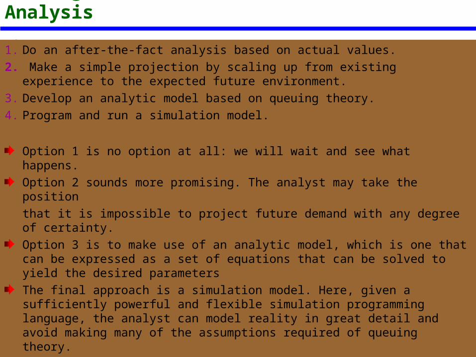
1. Do an after-the-fact analysis based on actual values.2. Make a simple projection by scaling up from existing experience to the expected

future environment.3. Develop an analytic model based on queuing theory.4. Program and run a simulation model.

Option 1 is no option at all: we will wait and see what happens.Option 2 sounds more promising. The analyst may take the positionthat it is impossible to project future demand with any degree of certainty.Option 3 is to make use of an analytic model, which is one that can be expressed as a set of equations that can be solved to yield the desired parametersThe final approach is a simulation model. Here, given a sufficiently powerful and flexible simulation programming language, the analyst can model reality in great detail and avoid making many of the assumptions required of queuing theory.

QUEUING MODELS

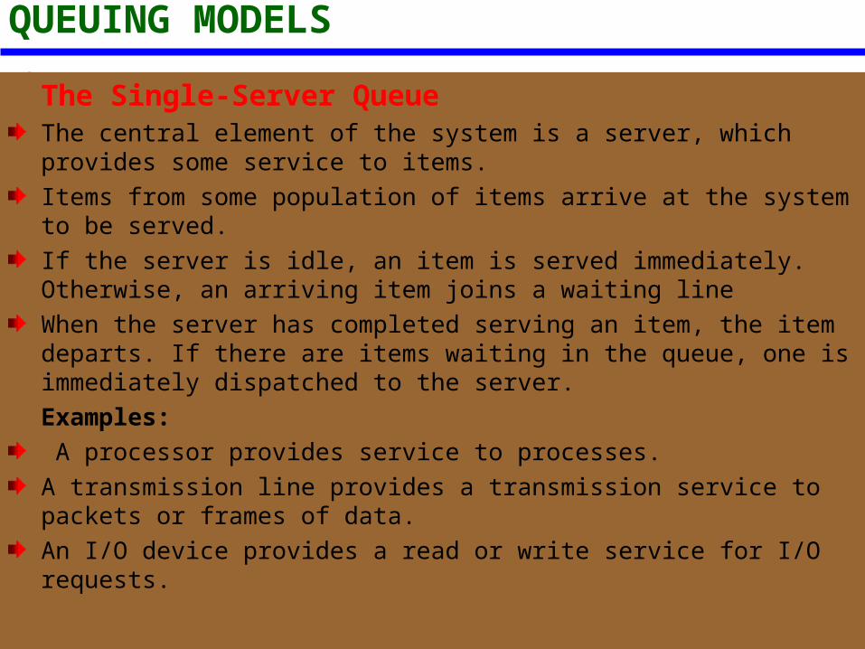
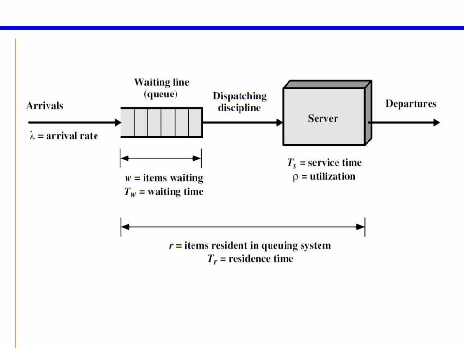
The Single-Server QueueThe central element of the system is a server, which provides some service to items.Items from some population of items arrive at the system to be served.If the server is idle, an item is served immediately. Otherwise, an arriving item joins a waiting lineWhen the server has completed serving an item, the item departs. If there are items waiting in the queue, one is immediately dispatched to the server.Examples: A processor provides service to processes.A transmission line provides a transmission service to packets or frames of data.An I/O device provides a read or write service for I/O requests.

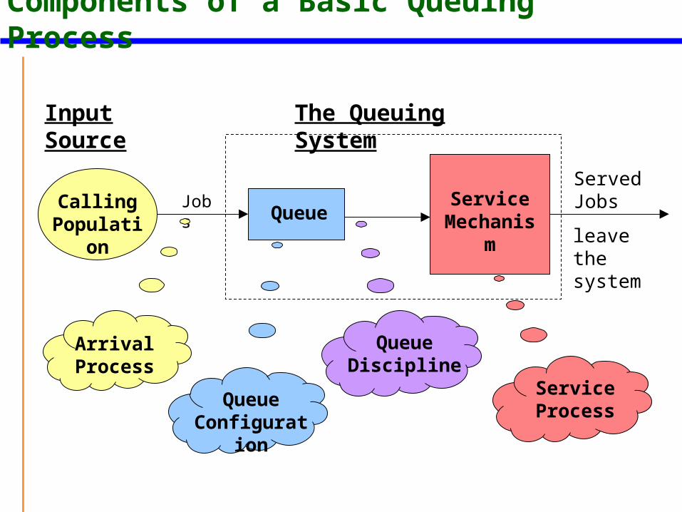
Components of a Basic Queuing Process

Calling Population Queue

Service Mechanism

Input Source The Queuing System

Jobs

Arrival Process

Queue Configuration

Queue Discipline

Served Jobs

Service Process

leave the system

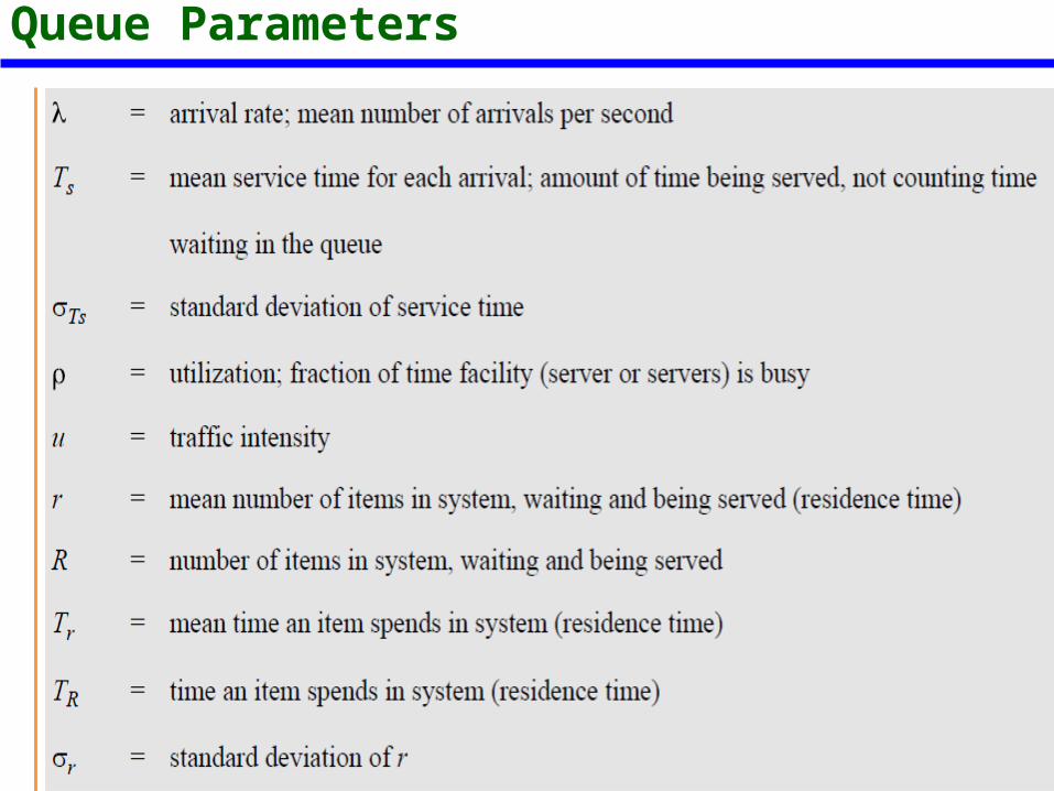
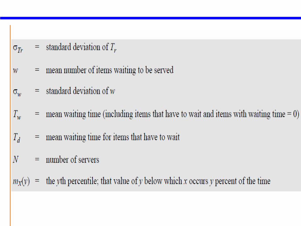
Queue Parameters

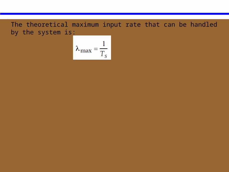
The theoretical maximum input rate that can be handled by the system is:

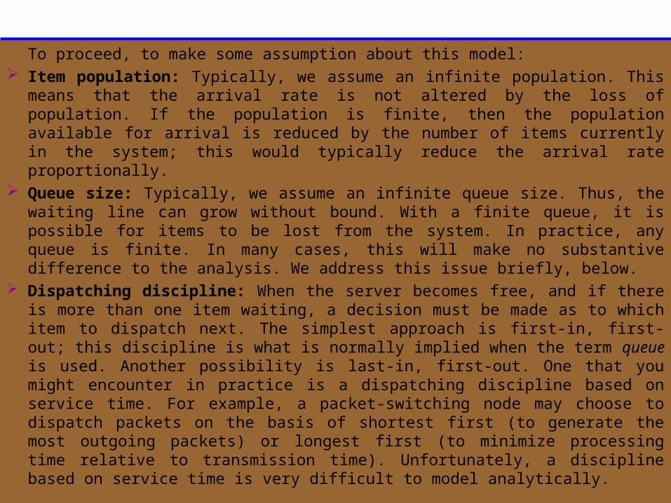
To proceed, to make some assumption about this model: Item population: Typically, we assume an infinite population. This means that the

arrival rate is not altered by the loss of population. If the population is finite, then the population available for arrival is reduced by the number of items currently in the system; this would typically reduce the arrival rate proportionally.

Queue size: Typically, we assume an infinite queue size. Thus, the waiting line can grow without bound. With a finite queue, it is possible for items to be lost from the system. In practice, any queue is finite. In many cases, this will make no substantive difference to the analysis. We address this issue briefly, below.

Dispatching discipline: When the server becomes free, and if there is more than one item waiting, a decision must be made as to which item to dispatch next. The simplest approach is first-in, first-out; this discipline is what is normally implied when the term queue is used. Another possibility is last-in, first-out. One that you might encounter in practice is a dispatching discipline based on service time. For example, a packet-switching node may choose to dispatch packets on the basis of shortest first (to generate the most outgoing packets) or longest first (to minimize processing time relative to transmission time). Unfortunately, a discipline based on service time is very difficult to model analytically.

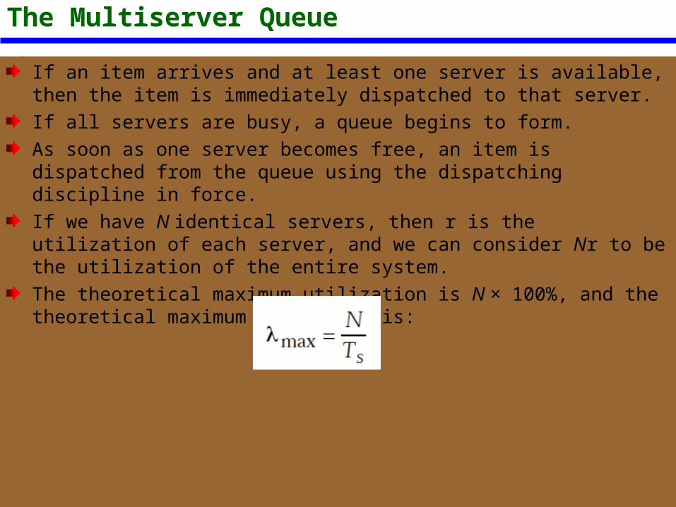
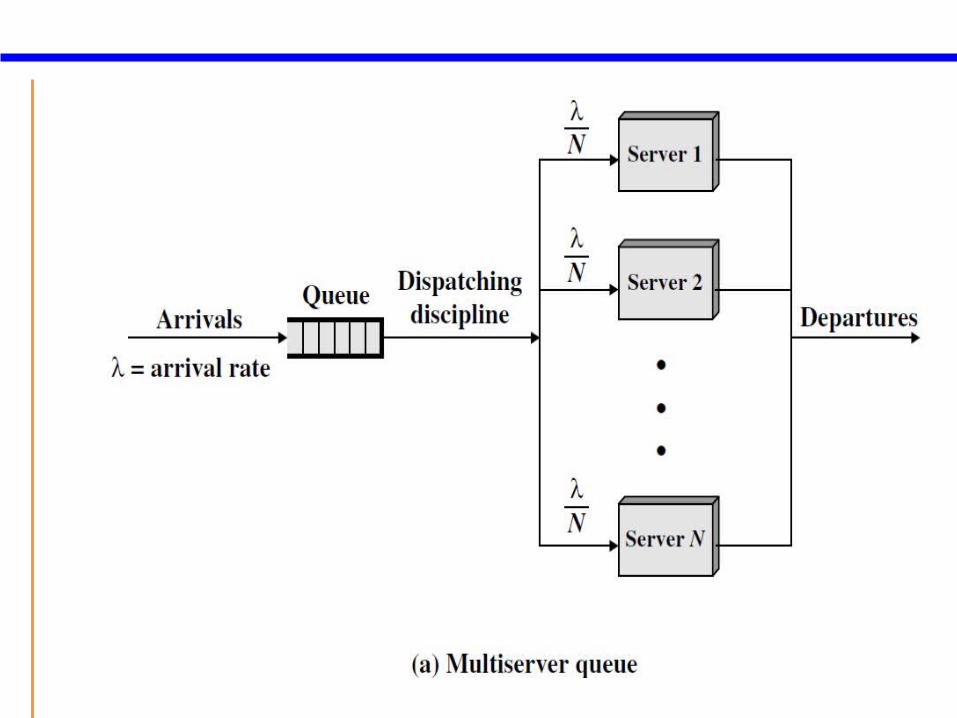
The Multiserver Queue

If an item arrives and at least one server is available, then the item is immediately dispatched to that server.If all servers are busy, a queue begins to form.As soon as one server becomes free, an item is dispatched from the queue using the dispatching discipline in force.If we have N identical servers, then r is the utilization of each server, and we can consider Nr to be the utilization of the entire system.The theoretical maximum utilization is N × 100%, and the theoretical maximum input rate is:

Basic Queuing Relationships

AssumptionsThe fundamental task of a queuing analysis is as follows: Given the following information asinput:Arrival rateService timeProvide as output information concerning:Items waitingWaiting timeItems in residenceResidence time.

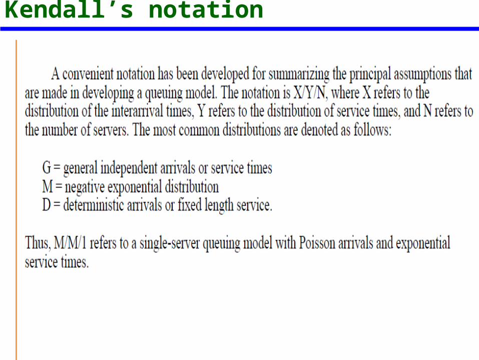
Kendall’s notation

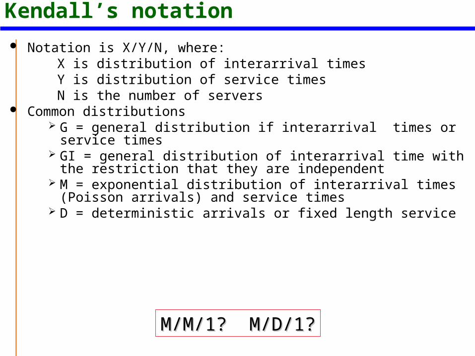
Kendall’s notation Notation is X/Y/N, where:

X is distribution of interarrival timesY is distribution of service timesN is the number of servers

Common distributions G = general distribution if interarrival times or service times GI = general distribution of interarrival time with the

restriction that they are independent M = exponential distribution of interarrival times (Poisson

arrivals) and service times D = deterministic arrivals or fixed length service

M/M/1? M/D/1?M/M/1? M/D/1?

Congestion and Traffic Management

What Is Congestion?

Congestion occurs when the number of packets being transmitted through the network approaches the packet handling capacity of the networkCongestion control aims to keep number of packets below level at which performance falls off dramaticallyData network is a network of queuesGenerally 80% utilization is criticalFinite queues mean data may be lost

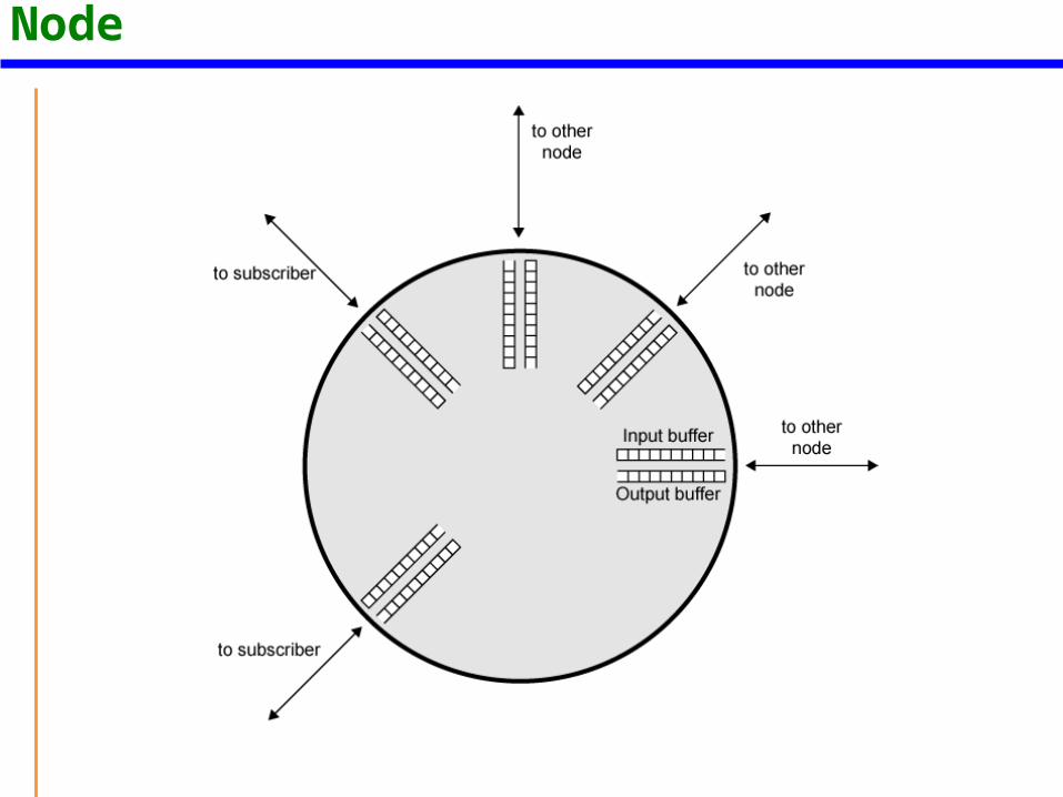
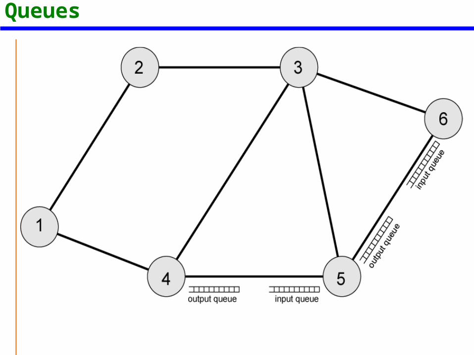
Queues at a Node

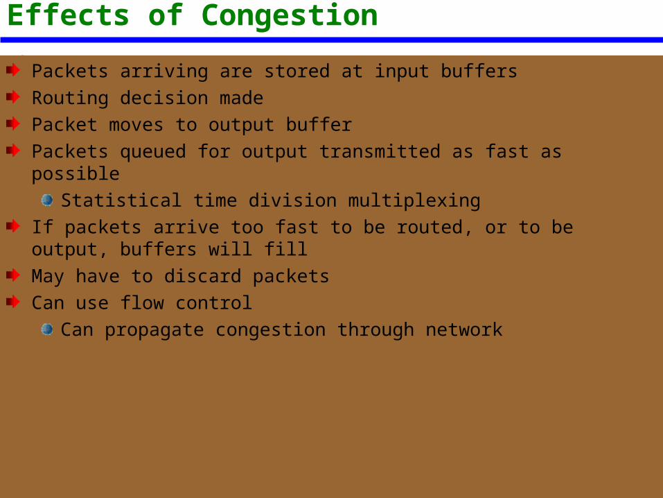
Effects of Congestion

Packets arriving are stored at input buffersRouting decision madePacket moves to output bufferPackets queued for output transmitted as fast as possible

Statistical time division multiplexingIf packets arrive too fast to be routed, or to be output, buffers will fillMay have to discard packetsCan use flow control

Can propagate congestion through network

Interaction of Queues

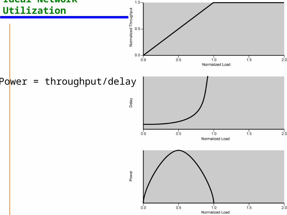
Ideal Network Utilization

Power = throughput/delay

Practical Performance

Ideal assumes infinite buffers and no overheadBuffers are finiteOverheads occur in exchanging congestion control messages

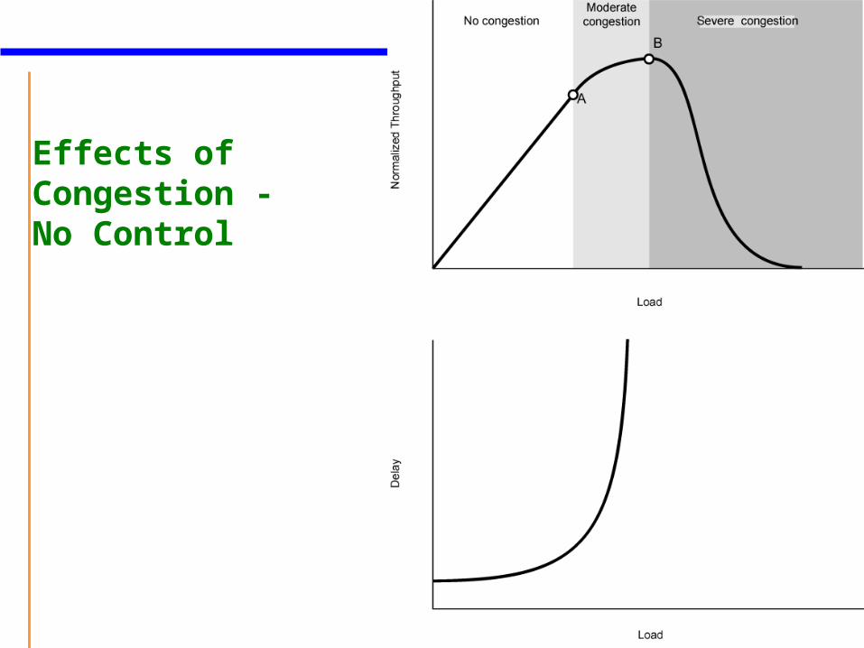
Effects of Congestion - No Control

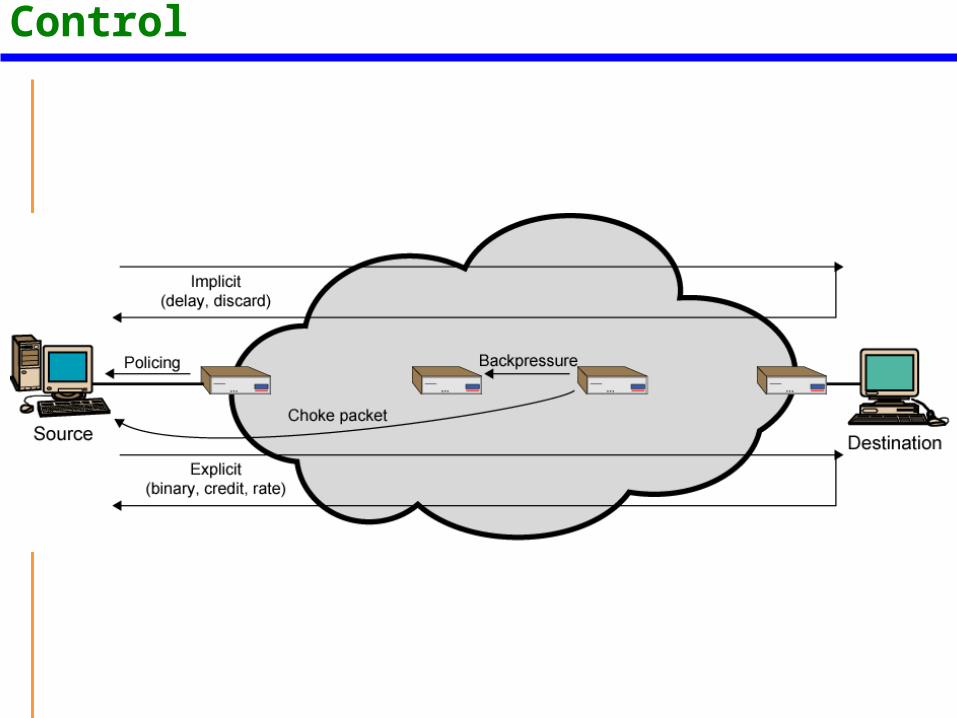
Mechanisms for Congestion Control

Backpressure

If node becomes congested it can slow down or halt flow of packets from other nodesMay mean that other nodes have to apply control on incoming packet ratesPropagates back to sourceCan restrict to logical connections generating most trafficUsed in connection oriented networks that allow hop by hop congestion control (e.g. X.25)

Choke Packet

Control packet Generated at congested nodeSent to source nodee.g. ICMP source quench

From router or destinationSource cuts back until no more source quench messageSent for every discarded packet, or anticipated

Rather crude mechanism

Implicit Congestion Signaling

Transmission delay may increase with congestionPacket may be discardedSource can detect these as implicit indications of congestionUseful on connectionless (datagram) networks

e.g. IP based(TCP includes congestion and flow control - see chapter 20)

Used in frame relay LAPF

Explicit Congestion Signaling

Network alerts end systems of increasing congestionEnd systems take steps to reduce offered loadBackwards

Congestion avoidance in opposite direction (toward the source)Forwards

Congestion avoidance in same direction (toward destination)The destination will echo the signal back to the source or the upper layer protocol will do some flow control

Categories of Explicit Signaling

BinaryA bit set in a packet indicates congestion

Credit basedIndicates how many packets source may sendCommon for end to end flow control

Rate basedSupply explicit data rate limite.g. ATM

Traffic Management

FairnessQuality of service

May want different treatment for different connectionsReservations

e.g. ATMTraffic contract between user and network

Congestion Control in Packet Switched Networks

Send control packet (e.g. choke packet) to some or all source nodesRequires additional traffic during congestion

Rely on routing informationMay react too quickly

End to end probe packetsAdds to overhead

Add congestion info to packets as they cross nodesEither backwards or forwards

Frame Relay Congestion Control Minimize discardsMaintain agreed QoSMinimize probability of one end user monopolySimple to implement

Little overhead on network or userCreate minimal additional trafficDistribute resources fairlyLimit spread of congestionOperate effectively regardless of traffic flowMinimum impact on other systemsMinimize variance in QoS

Techniques

Discard strategyCongestion avoidanceExplicit signalingCongestion recoveryImplicit signaling mechanism

Traffic Rate Management

Must discard frames to cope with congestionArbitrarily, no regard for sourceNo reward for restraint so end systems transmit as fast as possibleCommitted information rate (CIR)

Data in excess of this rate is liable to discardNot guaranteedAggregate CIR should not exceed physical data rate

Committed burst size (Bc)Excess burst size (Be)

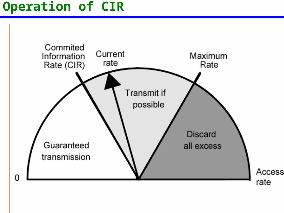
Operation of CIR

Relationship Among Congestion Parameters

Explicit Signaling

Network alerts end systems of growing congestionBackward explicit congestion notificationForward explicit congestion notificationFrame handler monitors its queuesMay notify some or all logical connectionsUser response

Reduce rate

UNIT III

TCP Traffic Control

Introduction

TCP Flow ControlTCP Congestion ControlPerformance of TCP over ATM

TCP Flow Control

Uses a form of sliding windowDiffers from mechanism used in LLC, HDLC, X.25, and others:

Decouples acknowledgement of received data units from granting permission to send more

TCP’s flow control is known as a credit allocation scheme:Each transmitted octet is considered to have a sequence number

TCP Header Fields for Flow ControlSequence number (SN) of first octet in data segmentAcknowledgement number (AN)Window (W)Acknowledgement contains AN = i, W = j:

Octets through SN = i - 1 acknowledgedPermission is granted to send W = j more octets,

i.e., octets i through i + j - 1

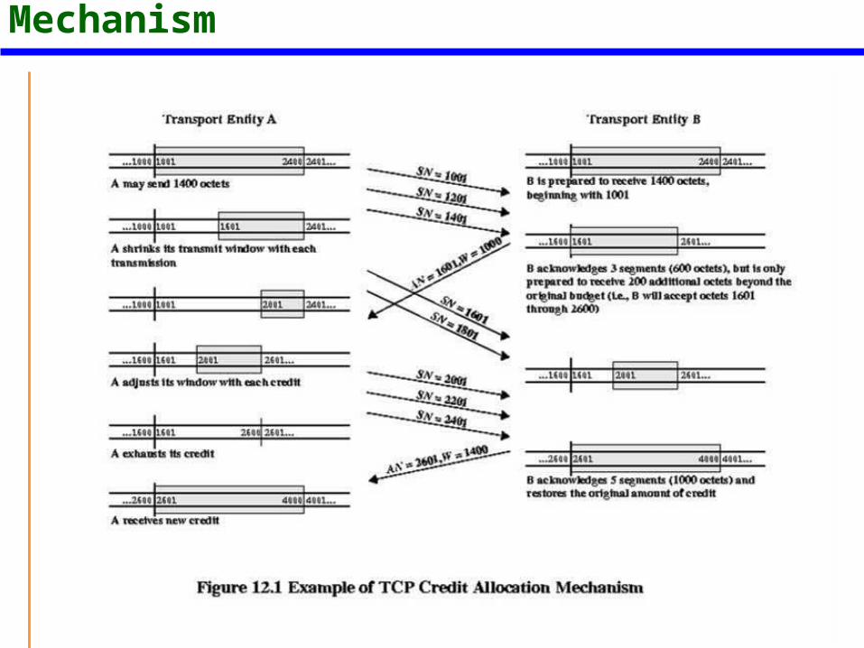
TCP Credit Allocation Mechanism

Credit Allocation is Flexible

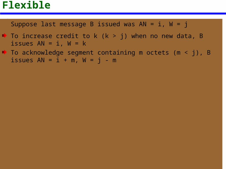
Suppose last message B issued was AN = i, W = j

To increase credit to k (k > j) when no new data, B issues AN = i, W = kTo acknowledge segment containing m octets (m < j), B issues AN = i + m, W = j - m

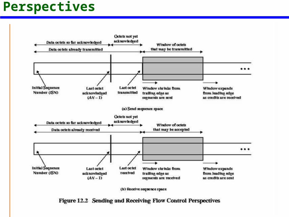
Figure 12.2 Flow Control Perspectives

Credit PolicyReceiver needs a policy for how much credit to give senderConservative approach: grant credit up to limit of available buffer spaceMay limit throughput in long-delay situationsOptimistic approach: grant credit based on expectation of freeing space before data arrives

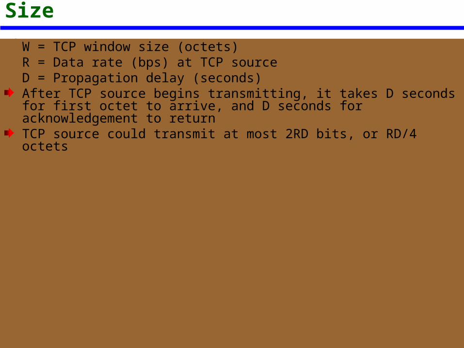
Effect of Window SizeW = TCP window size (octets)R = Data rate (bps) at TCP sourceD = Propagation delay (seconds)After TCP source begins transmitting, it takes D seconds for first octet to arrive, and D seconds for acknowledgement to returnTCP source could transmit at most 2RD bits, or RD/4 octets

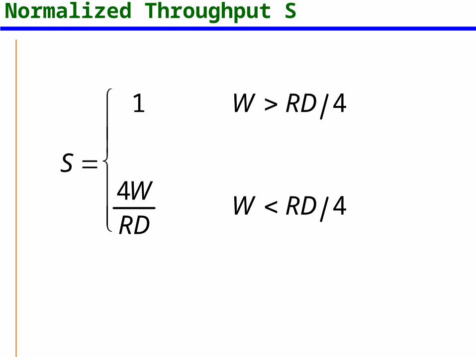
Normalized Throughput S

S

1 W RD 4

4WRD

W RD 4

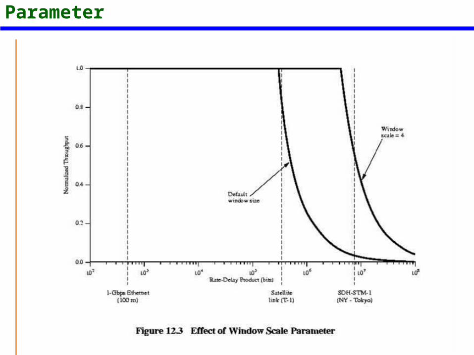
Window Scale Parameter

Complicating FactorsMultiple TCP connections are multiplexed over same network interface, reducing R and efficiencyFor multi-hop connections, D is the sum of delays across each network plus delays at each routerIf source data rate R exceeds data rate on one of the hops, that hop will be a bottleneckLost segments are retransmitted, reducing throughput. Impact depends on retransmission policy

Retransmission StrategyTCP relies exclusively on positive acknowledgements and retransmission on acknowledgement timeoutThere is no explicit negative acknowledgementRetransmission required when:

1. Segment arrives damaged, as indicated by checksum error, causing receiver to discard segment

2. Segment fails to arrive

Timers

A timer is associated with each segment as it is sentIf timer expires before segment acknowledged, sender must retransmitKey Design Issue:

value of retransmission timerToo small: many unnecessary retransmissions, wasting network bandwidthToo large: delay in handling lost segment

Two Strategies

Timer should be longer than round-trip delay (send segment, receive ack)Delay is variable

Strategies:1. Fixed timer2. Adaptive

Problems with Adaptive Scheme

Peer TCP entity may accumulate acknowledgements and not acknowledge immediatelyFor retransmitted segments, can’t tell whether acknowledgement is response to original transmission or retransmissionNetwork conditions may change suddenly

Adaptive Retransmission Timer

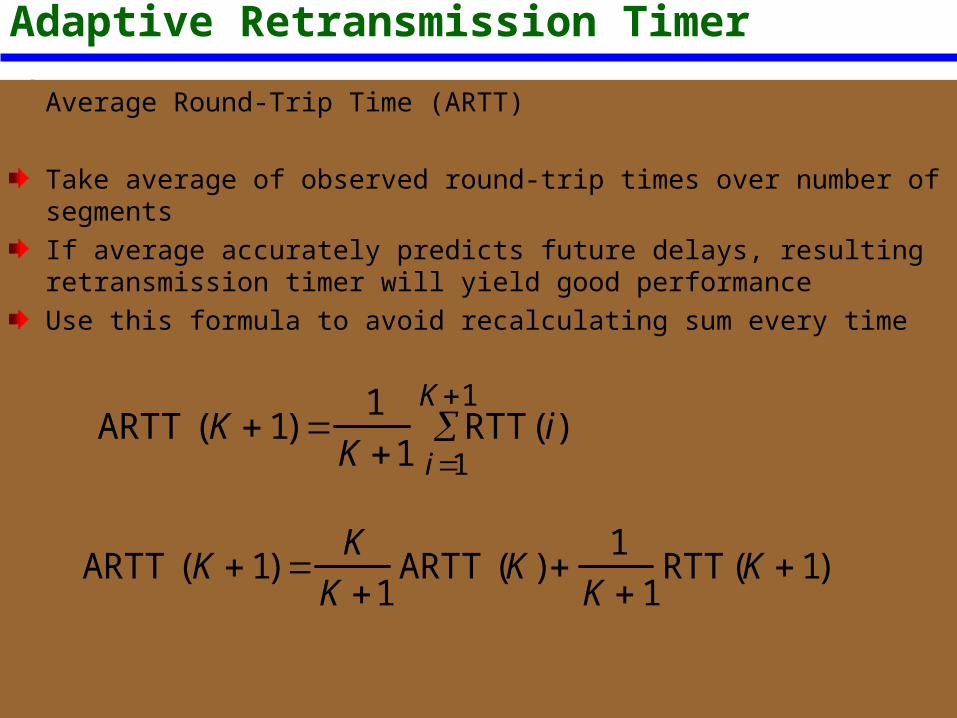
Average Round-Trip Time (ARTT)

Take average of observed round-trip times over number of segmentsIf average accurately predicts future delays, resulting retransmission timer will yield good performanceUse this formula to avoid recalculating sum every time

ARTT(K 1)

1K1

RTT(i)i1

K1

ARTT(K 1)

KK 1

ARTT(K) 1K1

RTT(K1)

RFC 793 Exponential Averaging

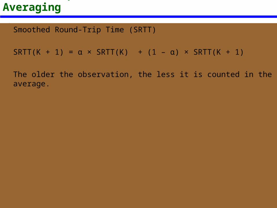
Smoothed Round-Trip Time (SRTT)

SRTT(K + 1) = α × SRTT(K) + (1 – α) × SRTT(K + 1)

The older the observation, the less it is counted in the average.

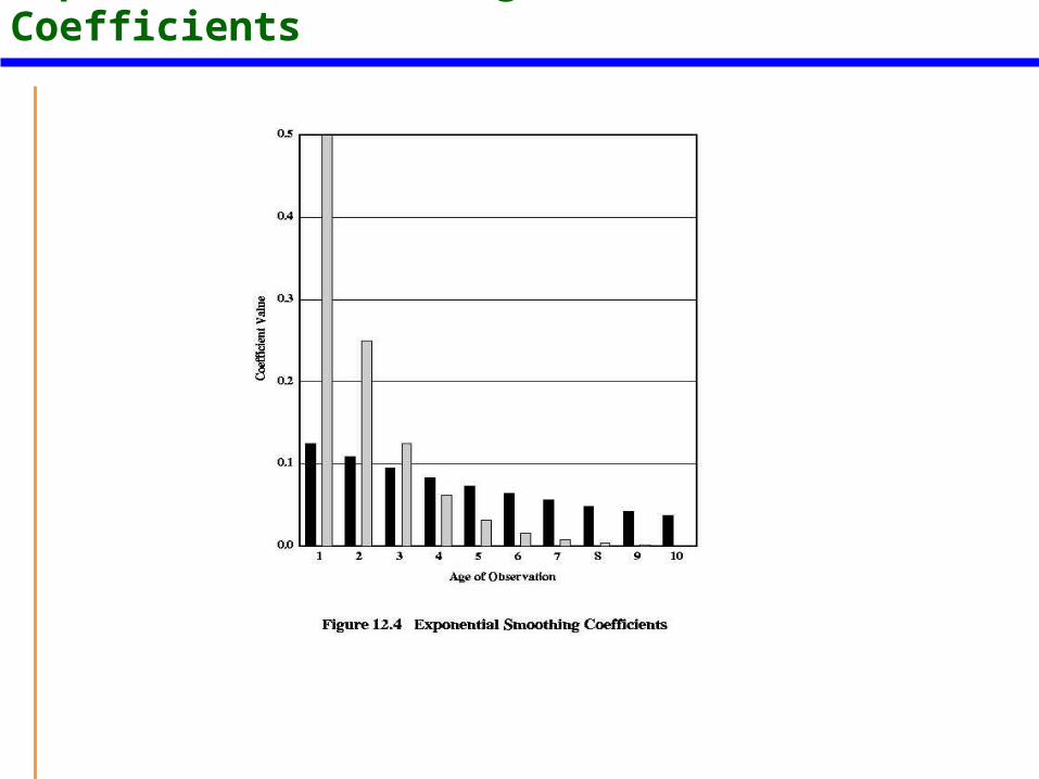
Exponential Smoothing Coefficients

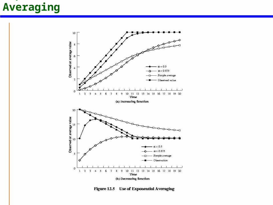
Exponential Averaging

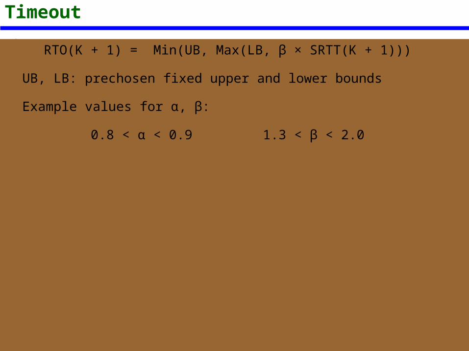
RFC 793 Retransmission Timeout

RTO(K + 1) = Min(UB, Max(LB, β × SRTT(K + 1)))

UB, LB: prechosen fixed upper and lower bounds

Example values for α, β:

0.8 < α < 0.9 1.3 < β < 2.0

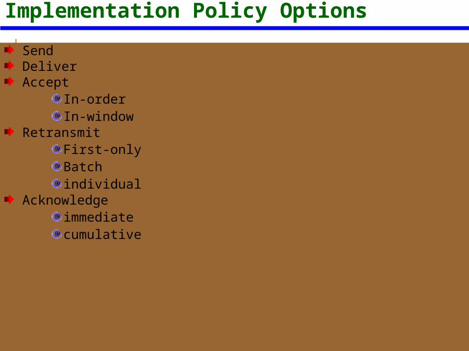
Implementation Policy Options

SendDeliverAccept

In-orderIn-window

RetransmitFirst-onlyBatchindividual

Acknowledgeimmediatecumulative

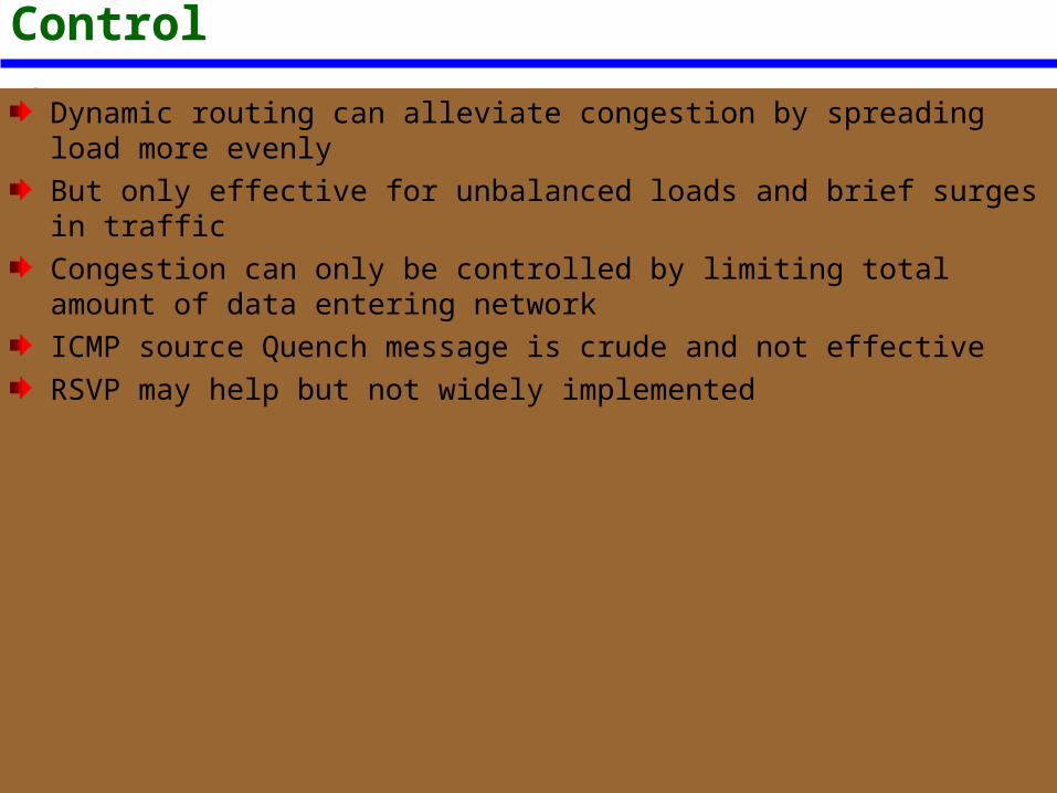
TCP Congestion Control

Dynamic routing can alleviate congestion by spreading load more evenlyBut only effective for unbalanced loads and brief surges in trafficCongestion can only be controlled by limiting total amount of data entering networkICMP source Quench message is crude and not effectiveRSVP may help but not widely implemented

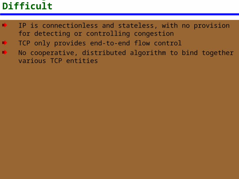
TCP Congestion Control is Difficult

IP is connectionless and stateless, with no provision for detecting or controlling congestionTCP only provides end-to-end flow controlNo cooperative, distributed algorithm to bind together various TCP entities

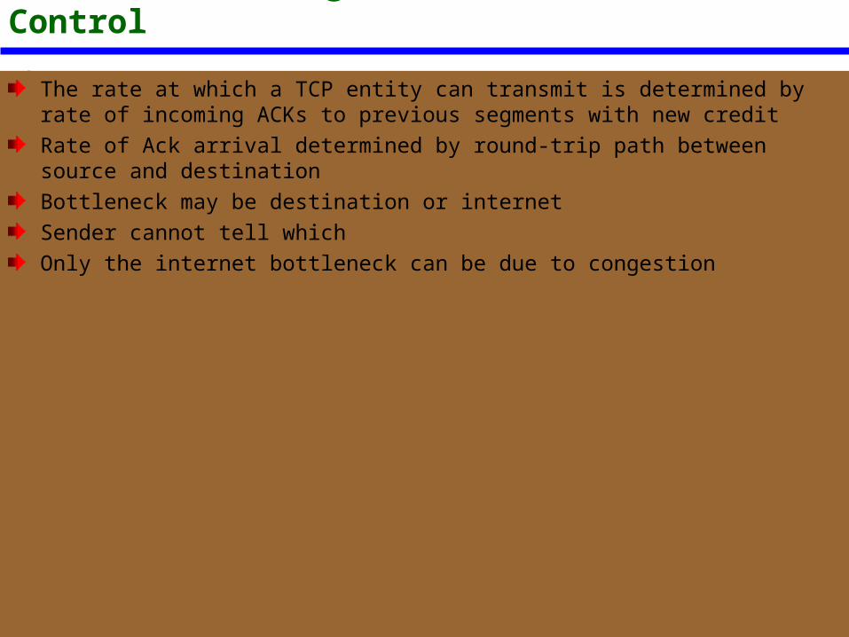
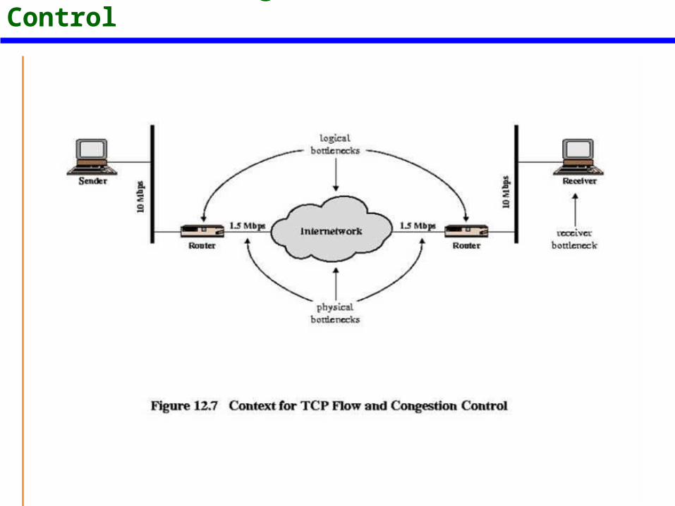
TCP Flow and Congestion Control

The rate at which a TCP entity can transmit is determined by rate of incoming ACKs to previous segments with new creditRate of Ack arrival determined by round-trip path between source and destinationBottleneck may be destination or internetSender cannot tell whichOnly the internet bottleneck can be due to congestion

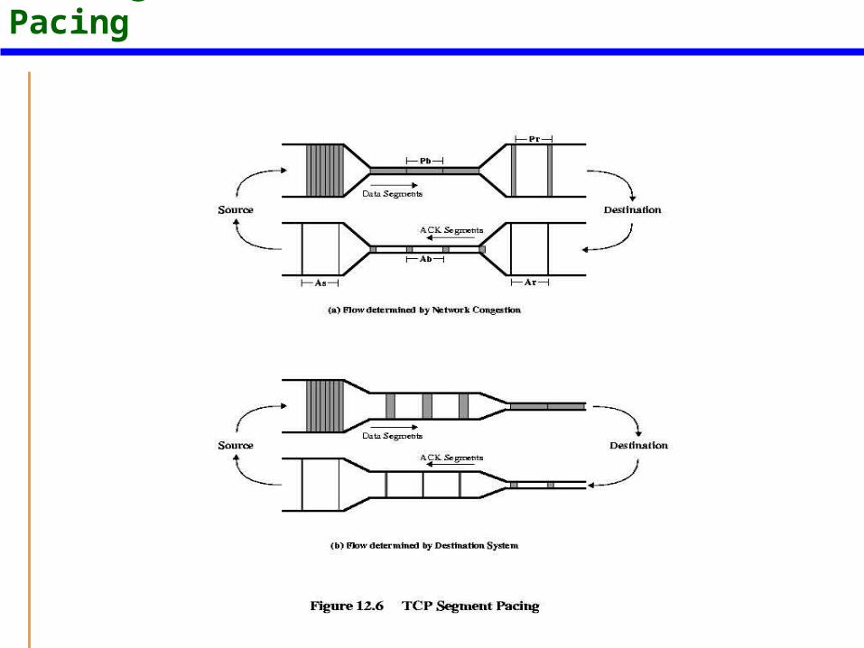
TCP Segment Pacing

TCP Flow and Congestion Control

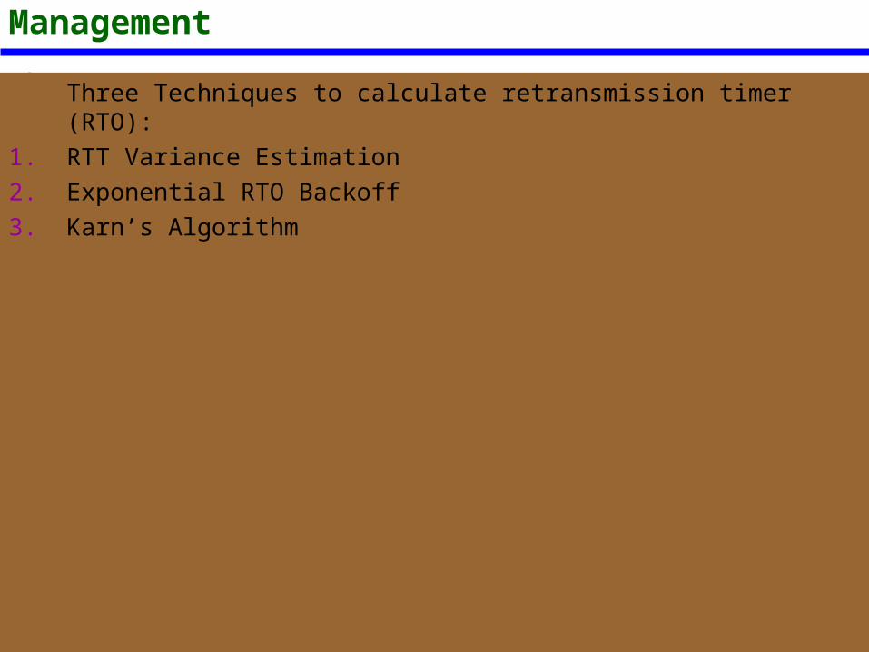
Retransmission Timer Management

Three Techniques to calculate retransmission timer (RTO):1. RTT Variance Estimation2. Exponential RTO Backoff3. Karn’s Algorithm

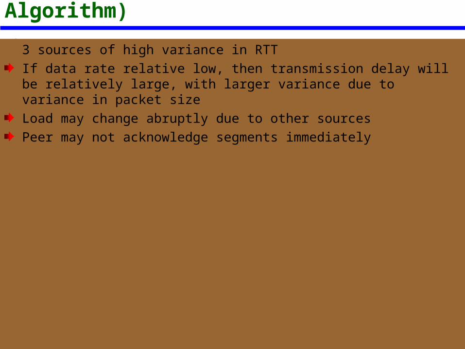
RTT Variance Estimation (Jacobson’s Algorithm)

3 sources of high variance in RTTIf data rate relative low, then transmission delay will be relatively large, with larger variance due to variance in packet sizeLoad may change abruptly due to other sourcesPeer may not acknowledge segments immediately

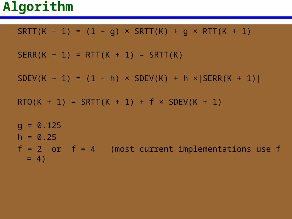
Jacobson’s Algorithm

SRTT(K + 1) = (1 – g) × SRTT(K) + g × RTT(K + 1)

SERR(K + 1) = RTT(K + 1) – SRTT(K)

SDEV(K + 1) = (1 – h) × SDEV(K) + h ×|SERR(K + 1)|

RTO(K + 1) = SRTT(K + 1) + f × SDEV(K + 1)

g = 0.125 h = 0.25 f = 2 or f = 4 (most current implementations use f = 4)

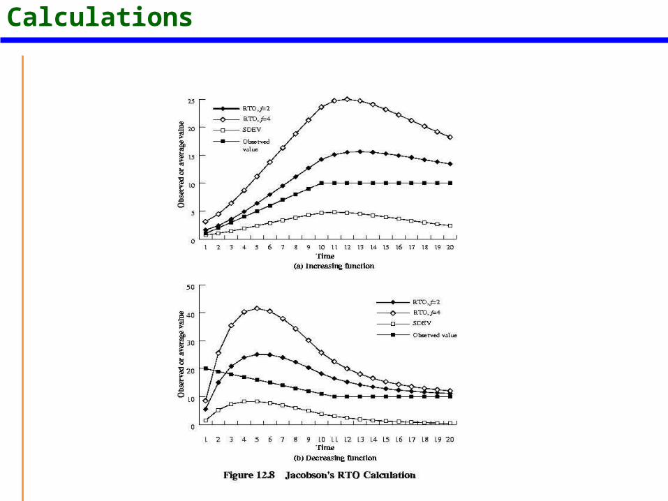
Jacobson’s RTO Calculations

Two Other Factors

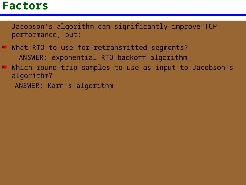
Jacobson’s algorithm can significantly improve TCP performance, but:

What RTO to use for retransmitted segments? ANSWER: exponential RTO backoff algorithm

Which round-trip samples to use as input to Jacobson’s algorithm?ANSWER: Karn’s algorithm

Exponential RTO Backoff

Increase RTO each time the same segment retransmitted – backoff processMultiply RTO by constant:

RTO = q × RTOq = 2 is called binary exponential backoff

Which Round-trip Samples?

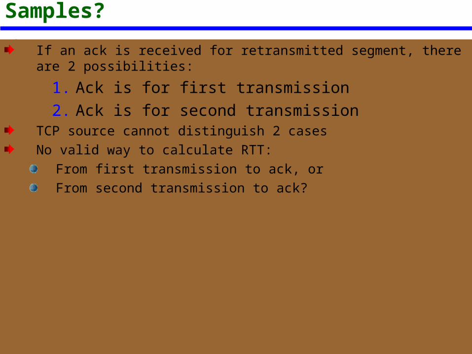
If an ack is received for retransmitted segment, there are 2 possibilities:

1. Ack is for first transmission2. Ack is for second transmission

TCP source cannot distinguish 2 casesNo valid way to calculate RTT:

From first transmission to ack, orFrom second transmission to ack?

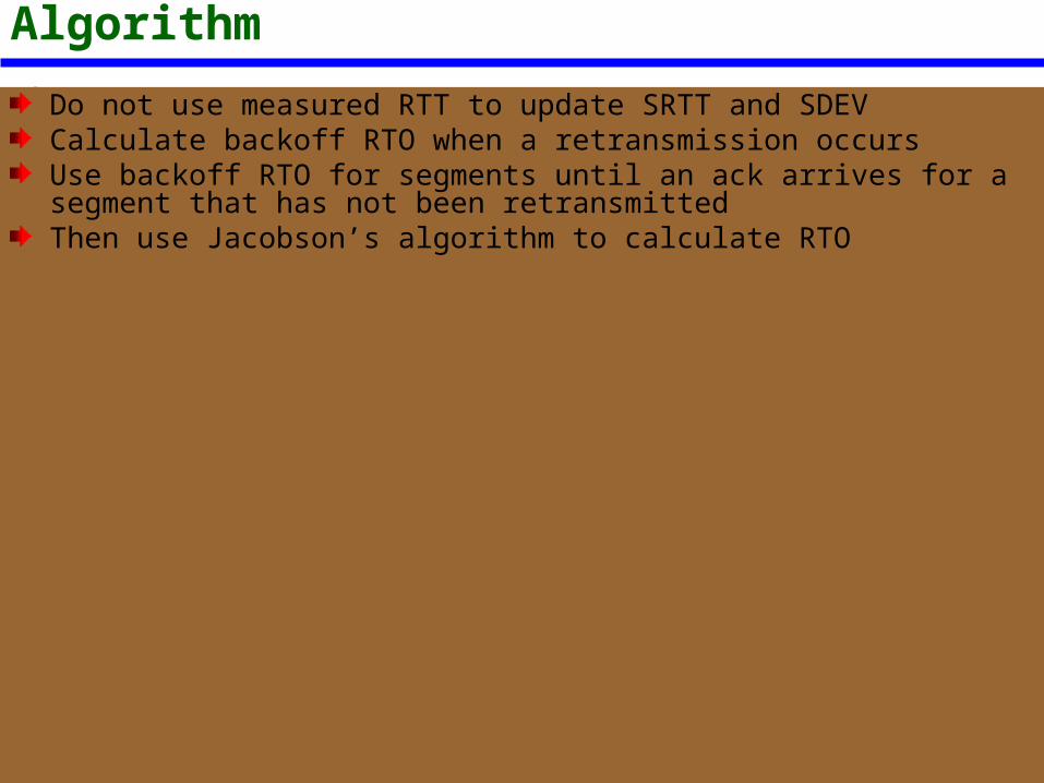
Karn’s AlgorithmDo not use measured RTT to update SRTT and SDEVCalculate backoff RTO when a retransmission occursUse backoff RTO for segments until an ack arrives for a segment that has not been retransmittedThen use Jacobson’s algorithm to calculate RTO

Window Management

Slow startDynamic window sizing on congestionFast retransmitFast recoveryLimited transmit

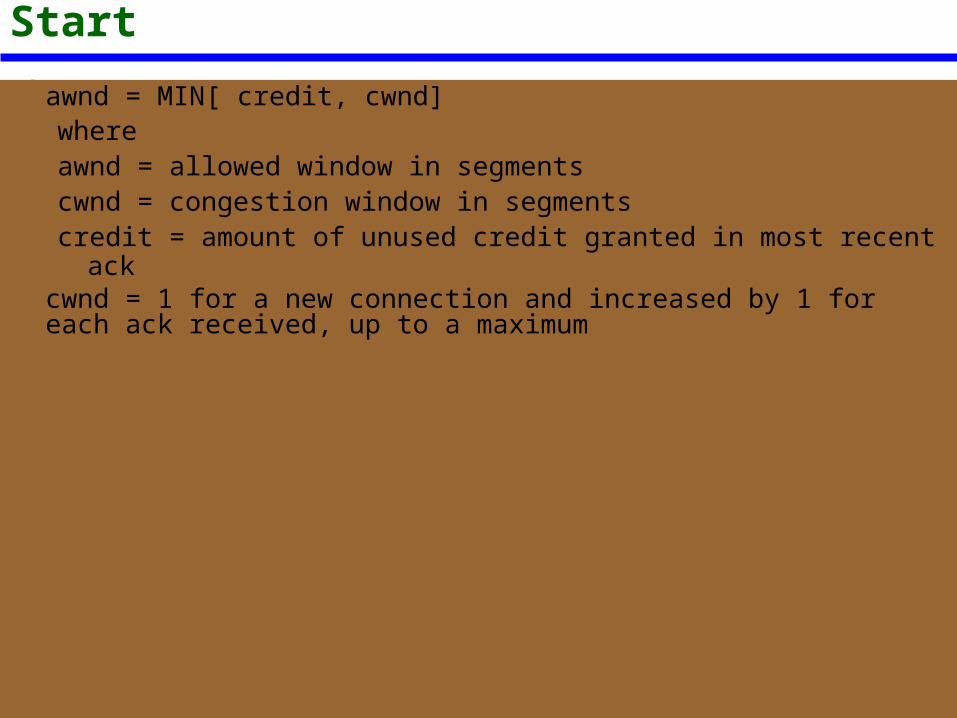
Slow Startawnd = MIN[ credit, cwnd]whereawnd = allowed window in segmentscwnd = congestion window in segmentscredit = amount of unused credit granted in most recent ack

cwnd = 1 for a new connection and increased by 1 for each ack received, up to a maximum

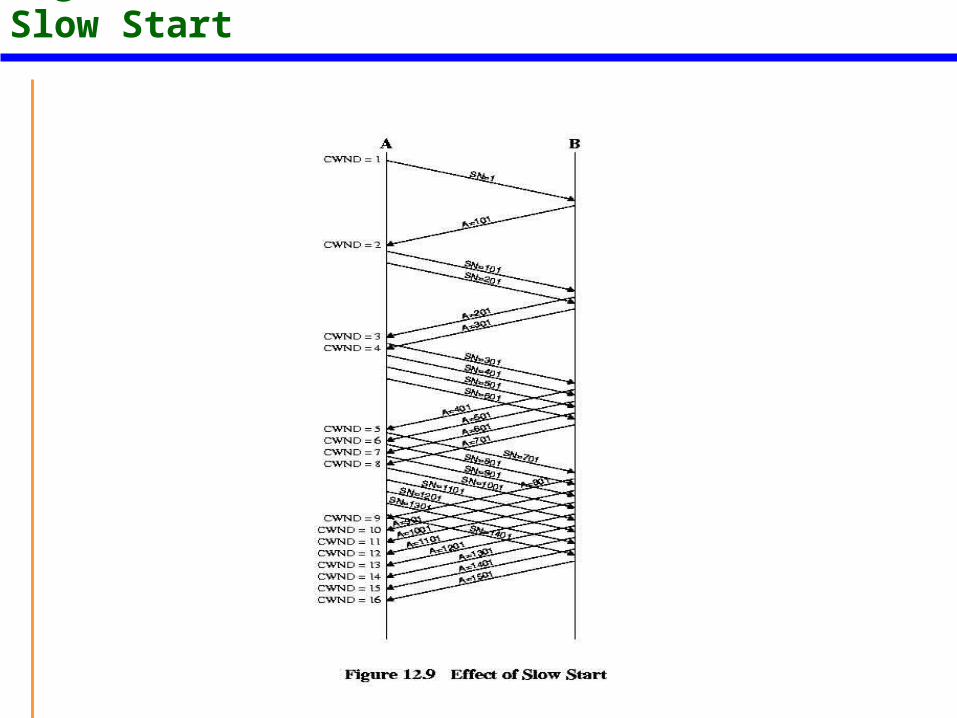
Figure 23.9 Effect of Slow Start

Dynamic Window Sizing on Congestion

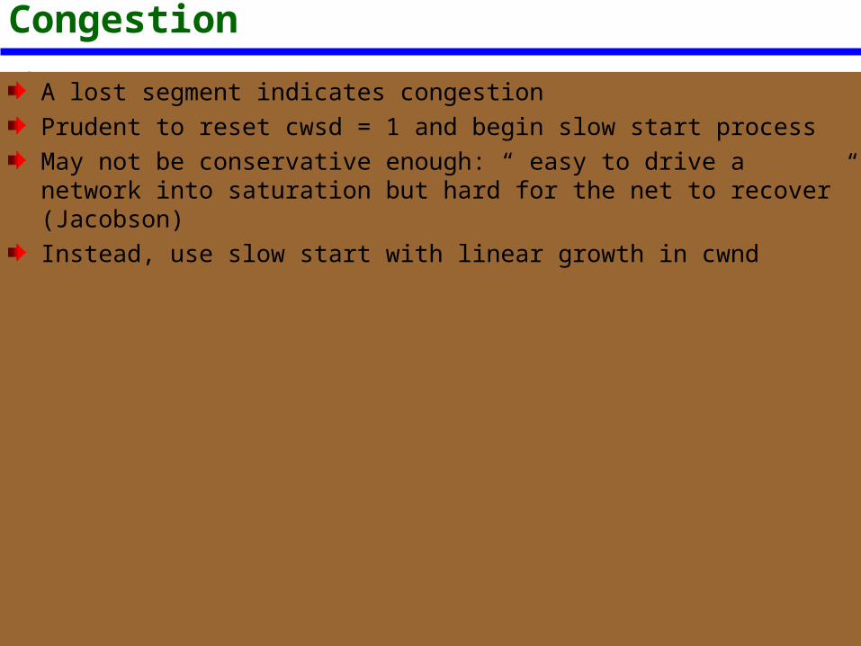
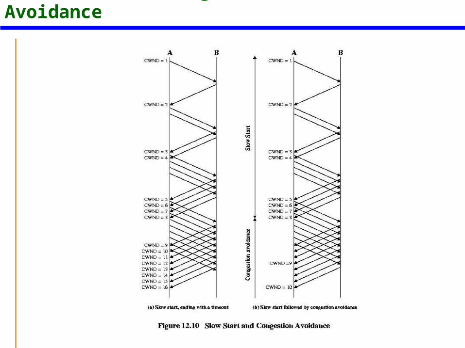
A lost segment indicates congestionPrudent to reset cwsd = 1 and begin slow start processMay not be conservative enough: “ easy to drive a network into saturation but hard for the net to recover” (Jacobson)Instead, use slow start with linear growth in cwnd

Slow Start and Congestion Avoidance

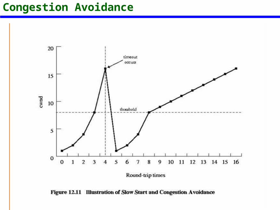
Illustration of Slow Start and Congestion Avoidance

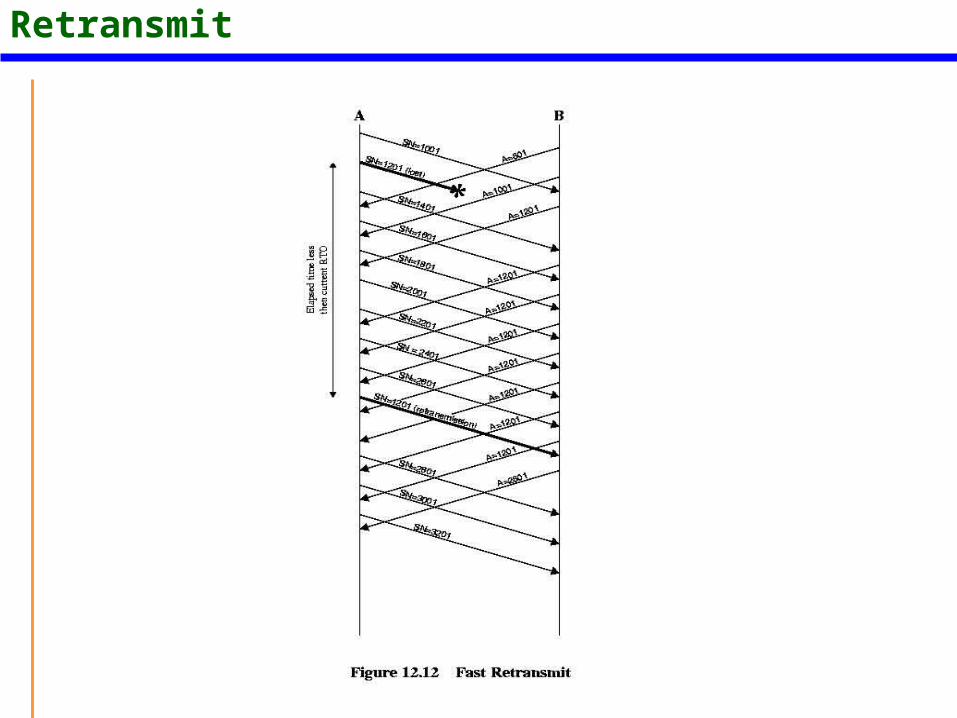
Fast RetransmitRTO is generally noticeably longer than actual RTTIf a segment is lost, TCP may be slow to retransmitTCP rule: if a segment is received out of order, an ack must be issued immediately for the last in-order segmentFast Retransmit rule: if 4 acks received for same segment, highly likely it was lost, so retransmit immediately, rather than waiting for timeout

Fast Retransmit

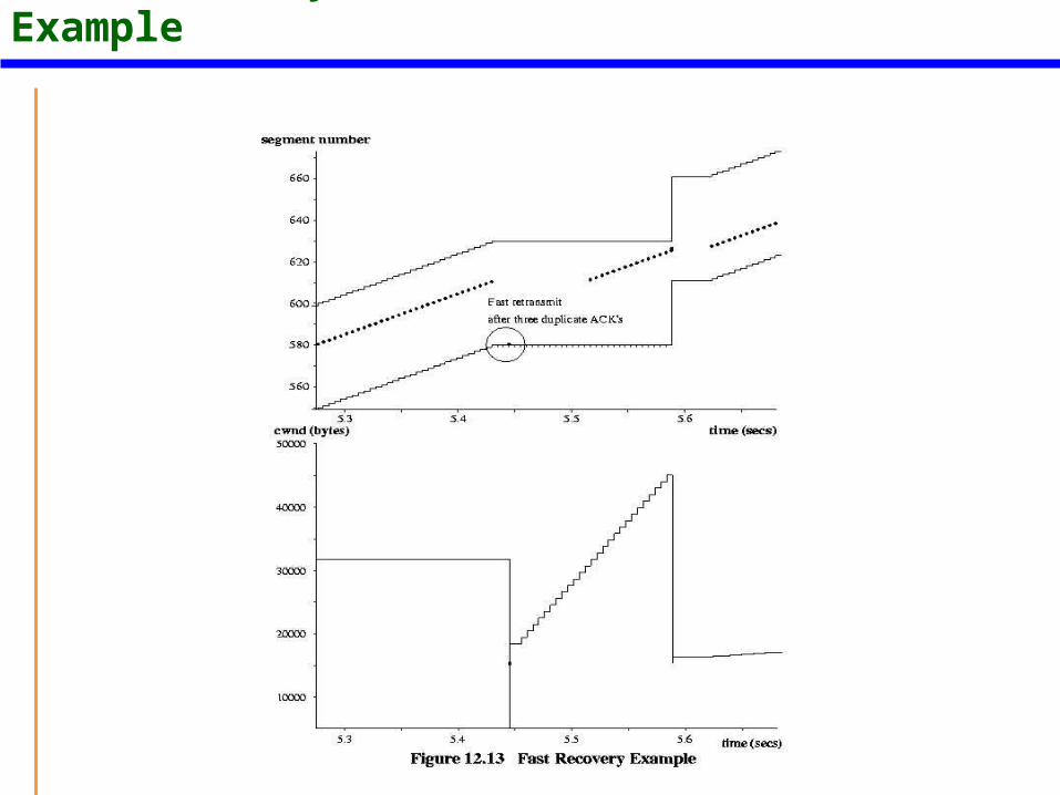
Fast RecoveryWhen TCP retransmits a segment using Fast Retransmit, a segment was assumed lostCongestion avoidance measures are appropriate at this pointE.g., slow-start/congestion avoidance procedureThis may be unnecessarily conservative since multiple acks indicate segments are getting throughFast Recovery: retransmit lost segment, cut cwnd in half, proceed with linear increase of cwndThis avoids initial exponential slow-start

Fast Recovery Example

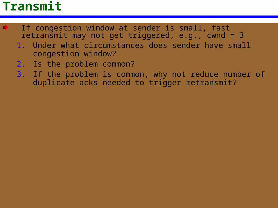
Limited TransmitIf congestion window at sender is small, fast retransmit may not get triggered, e.g., cwnd = 3

1. Under what circumstances does sender have small congestion window?2. Is the problem common?3. If the problem is common, why not reduce number of duplicate acks needed

to trigger retransmit?

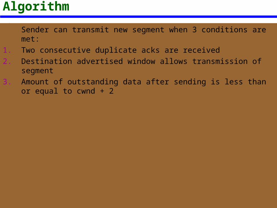
Limited Transmit Algorithm

Sender can transmit new segment when 3 conditions are met:1. Two consecutive duplicate acks are received2. Destination advertised window allows transmission of segment3. Amount of outstanding data after sending is less than or equal to cwnd + 2

Performance of TCP over ATM

How best to manage TCP’s segment size, window management and congestion control……at the same time as ATM’s quality of service and traffic control policiesTCP may operate end-to-end over one ATM network, or there may be multiple ATM LANs or WANs with non-ATM networks

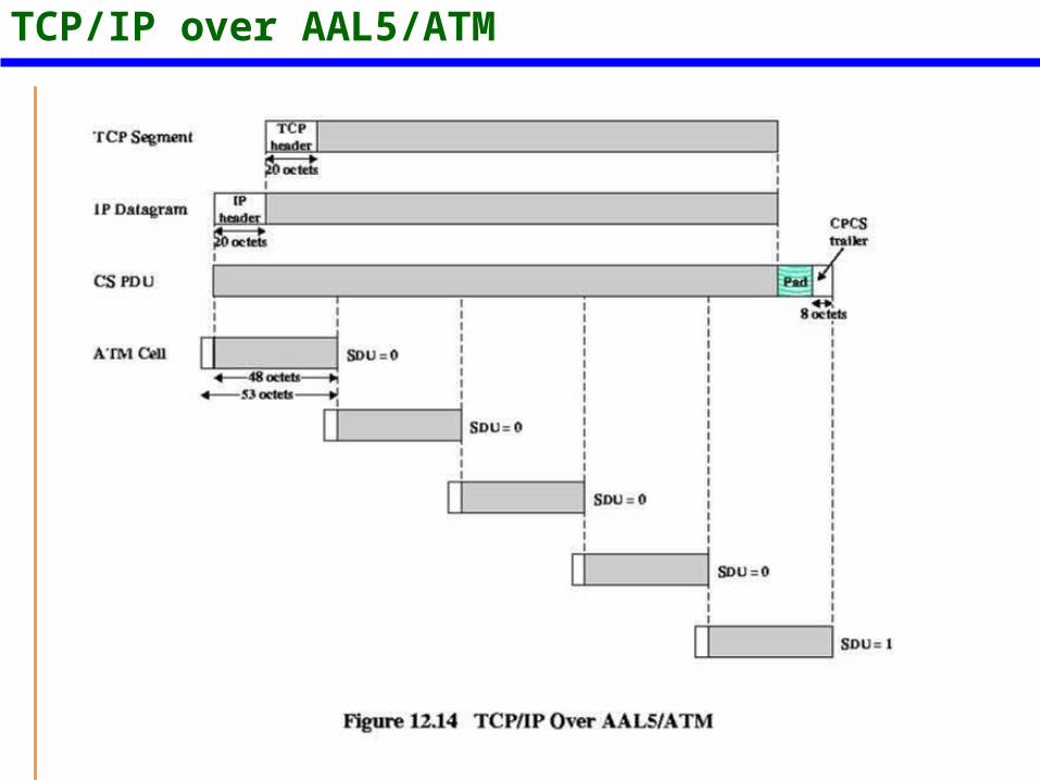
TCP/IP over AAL5/ATM

Performance of TCP over UBR

Buffer capacity at ATM switches is a critical parameter in assessing TCP throughput performanceInsufficient buffer capacity results in lost TCP segments and retransmissions

Effect of Switch Buffer Size

Data rate of 141 MbpsEnd-to-end propagation delay of 6 μsIP packet sizes of 512 octets to 9180TCP window sizes from 8 Kbytes to 64 KbytesATM switch buffer size per port from 256 cells to 8000One-to-one mapping of TCP connections to ATM virtual circuitsTCP sources have infinite supply of data ready

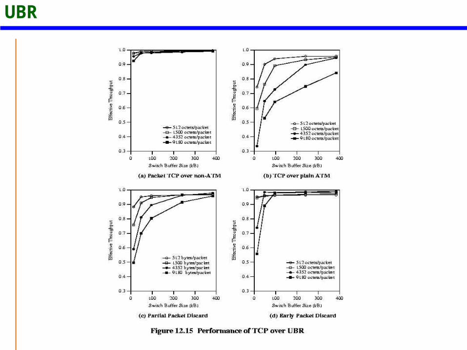
Performance of TCP over UBR

ObservationsIf a single cell is dropped, other cells in the same IP datagram are unusable, yet ATM network forwards these useless cells to destinationSmaller buffer increase probability of dropped cellsLarger segment size increases number of useless cells transmitted if a single cell dropped

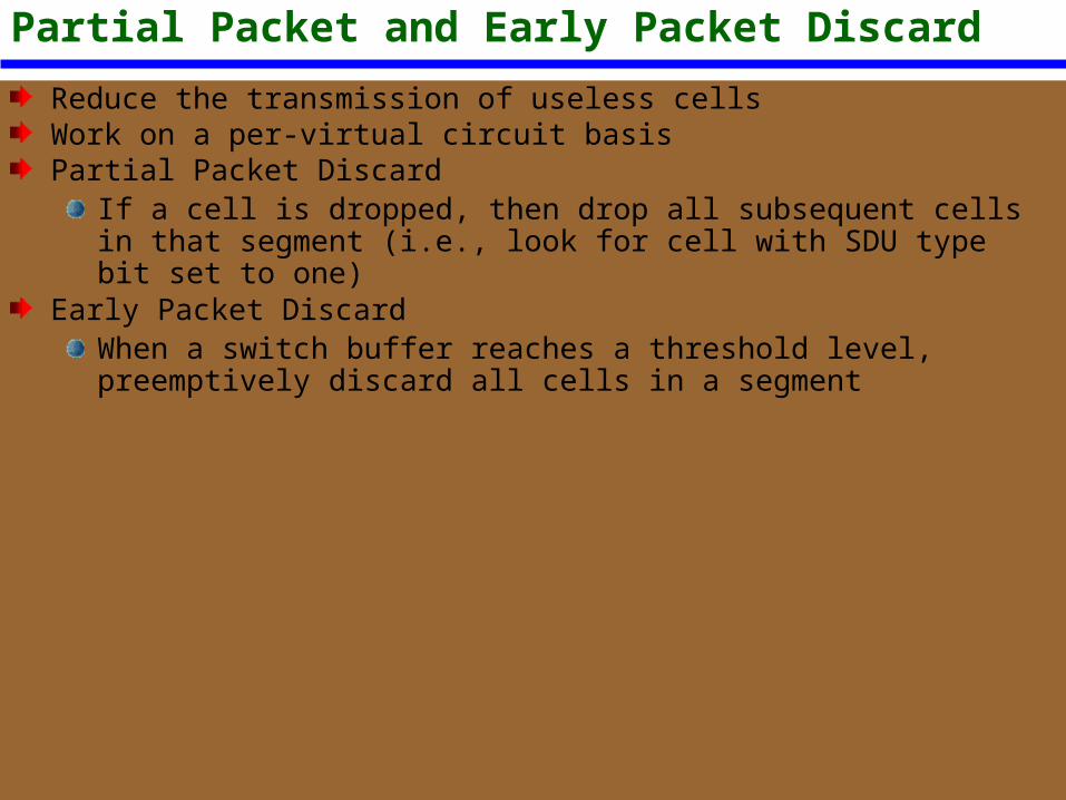
Partial Packet and Early Packet DiscardReduce the transmission of useless cellsWork on a per-virtual circuit basisPartial Packet Discard

If a cell is dropped, then drop all subsequent cells in that segment (i.e., look for cell with SDU type bit set to one)

Early Packet DiscardWhen a switch buffer reaches a threshold level, preemptively discard all cells in a segment

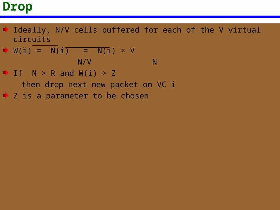
Selective Drop

Ideally, N/V cells buffered for each of the V virtual circuitsW(i) = N(i) = N(i) × V

N/V NIf N > R and W(i) > Z

then drop next new packet on VC i Z is a parameter to be chosen

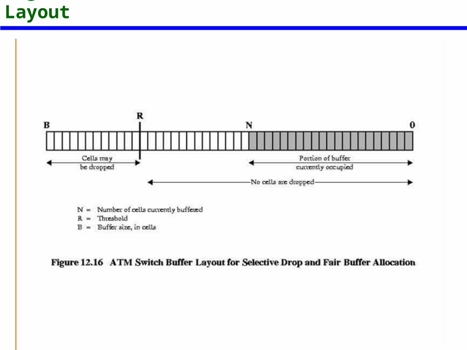
Figure 12.16 ATM Switch Buffer Layout

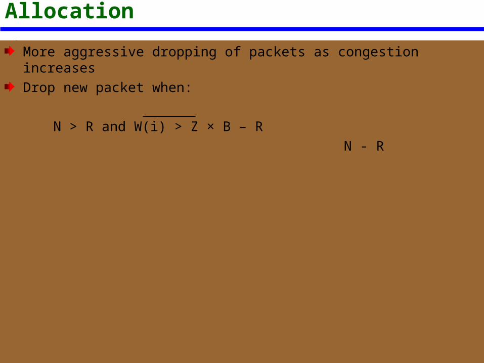
Fair Buffer Allocation

More aggressive dropping of packets as congestion increasesDrop new packet when:

N > R and W(i) > Z × B – R N - R

TCP over ABRGood performance of TCP over UBR can be achieved with minor adjustments to switch mechanismsThis reduces the incentive to use the more complex and more expensive ABR servicePerformance and fairness of ABR quite sensitive to some ABR parameter settingsOverall, ABR does not provide significant performance over simpler and less expensive UBR-EPD or UBR-EPD-FBA

Traffic and Congestion Control in ATM Networks

IntroductionControl needed to prevent switch buffer overflowHigh speed and small cell size gives different problems from other networksLimited number of overhead bitsITU-T specified restricted initial set

I.371ATM forum Traffic Management Specification 41

OverviewCongestion problemFramework adopted by ITU-T and ATM forum

Control schemes for delay sensitive trafficVoice & video

Not suited to bursty trafficTraffic controlCongestion control

Bursty trafficAvailable Bit Rate (ABR)Guaranteed Frame Rate (GFR)

Requirements for ATM Traffic and Congestion Control

Most packet switched and frame relay networks carry non-real-time bursty dataNo need to replicate timing at exit nodeSimple statistical multiplexingUser Network Interface capacity slightly greater than average of channels

Congestion control tools from these technologies do not work in ATM

Problems with ATM Congestion ControlMost traffic not amenable to flow control

Voice & video can not stop generatingFeedback slow

Small cell transmission time v propagation delayWide range of applications

From few kbps to hundreds of MbpsDifferent traffic patternsDifferent network services

High speed switching and transmissionVolatile congestion and traffic control

Key Performance Issues-Latency/Speed EffectsE.g. data rate 150MbpsTakes (53 x 8 bits)/(150 x 106) =2.8 x 10-6 seconds to insert a cellTransfer time depends on number of intermediate switches, switching time and propagation delay. Assuming no switching delay and speed of light propagation, round trip delay of 48 x 10-3 sec across USAA dropped cell notified by return message will arrive after source has transmitted N further cellsN=(48 x 10-3 seconds)/(2.8 x 10-6 seconds per cell)=1.7 x 104 cells = 7.2 x 106 bitsi.e. over 7 Mbits

Key Performance Issues-Cell Delay VariationFor digitized voice delay across network must be smallRate of delivery must be constantVariations will occurDealt with by Time Reassembly of CBR cells (see next slide)Results in cells delivered at CBR with occasional gaps due to dropped cellsSubscriber requests minimum cell delay variation from network provider

Increase data rate at UNI relative to loadIncrease resources within network

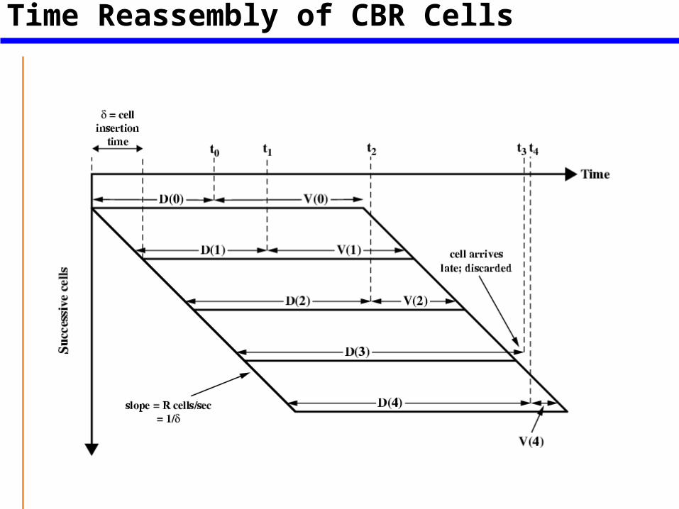
Time Reassembly of CBR Cells

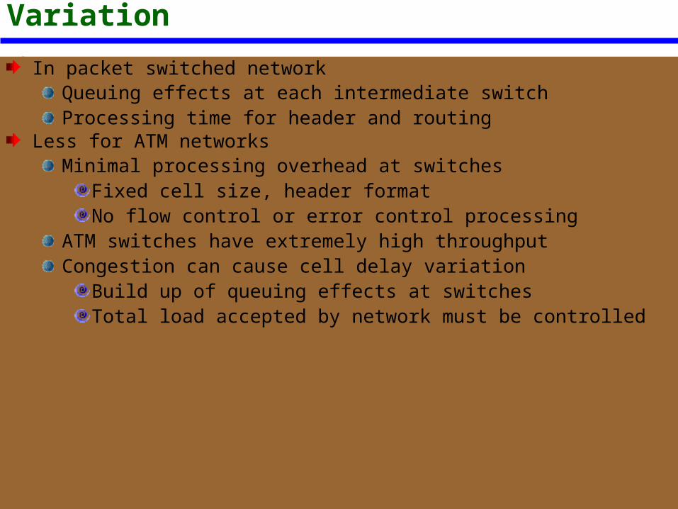
Network Contribution to Cell Delay VariationIn packet switched network

Queuing effects at each intermediate switchProcessing time for header and routing

Less for ATM networksMinimal processing overhead at switches

Fixed cell size, header formatNo flow control or error control processing

ATM switches have extremely high throughputCongestion can cause cell delay variation

Build up of queuing effects at switchesTotal load accepted by network must be controlled

Cell Delay Variation at UNI

Caused by processing in three layers of ATM modelSee next slide for details

None of these delays can be predictedNone follow repetitive patternSo, random element exists in time interval between reception by ATM stack and transmission

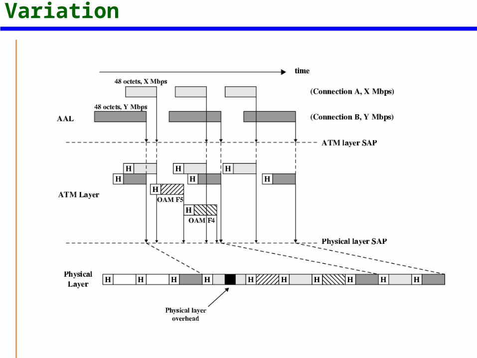
Origins of Cell Delay Variation

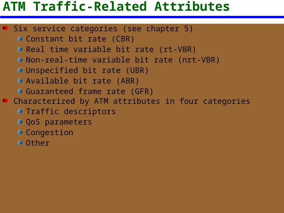
ATM Traffic-Related AttributesSix service categories (see chapter 5)

Constant bit rate (CBR)Real time variable bit rate (rt-VBR)Non-real-time variable bit rate (nrt-VBR)Unspecified bit rate (UBR)Available bit rate (ABR)Guaranteed frame rate (GFR)

Characterized by ATM attributes in four categoriesTraffic descriptorsQoS parametersCongestionOther

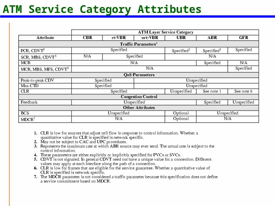
ATM Service Category Attributes

Traffic Parameters

Traffic pattern of flow of cellsIntrinsic nature of traffic

Source traffic descriptorModified inside network

Connection traffic descriptor

Source Traffic Descriptor (1)Peak cell rate

Upper bound on traffic that can be submittedDefined in terms of minimum spacing between cells TPCR = 1/TMandatory for CBR and VBR services

Sustainable cell rateUpper bound on average rateCalculated over large time scale relative to TRequired for VBREnables efficient allocation of network resources between VBR sourcesOnly useful if SCR < PCR

Source Traffic Descriptor (2)Maximum burst size

Max number of cells that can be sent at PCRIf bursts are at MBS, idle gaps must be enough to keep overall rate below SCRRequired for VBR

Minimum cell rateMin commitment requested of networkCan be zeroUsed with ABR and GFRABR & GFR provide rapid access to spare network capacity up to PCRPCR – MCR represents elastic component of data flowShared among ABR and GFR flows

Source Traffic Descriptor (3)

Maximum frame sizeMax number of cells in frame that can be carried over GFR connectionOnly relevant in GFR

Connection Traffic DescriptorIncludes source traffic descriptor plus:-Cell delay variation tolerance

Amount of variation in cell delay introduced by network interface and UNIBound on delay variability due to slotted nature of ATM, physical layer overhead and layer functions (e.g. cell multiplexing)Represented by time variable τ

Conformance definitionSpecify conforming cells of connection at UNIEnforced by dropping or marking cells over definition

Quality of Service Parameters- maxCTDCell transfer delay (CTD)

Time between transmission of first bit of cell at source and reception of last bit at destinationTypically has probability density function (see next slide)Fixed delay due to propagation etc.Cell delay variation due to buffering and schedulingMaximum cell transfer delay (maxCTD)is max requested delay for connectionFraction α of cells exceed threshold

Discarded or delivered late

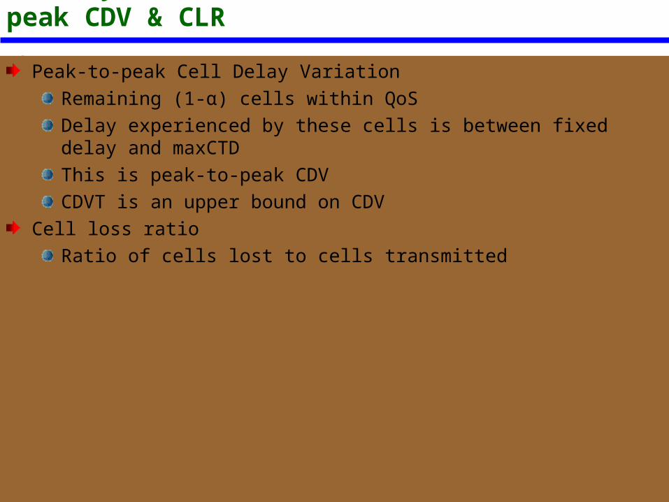
Quality of Service Parameters- Peak-to-peak CDV & CLR

Peak-to-peak Cell Delay VariationRemaining (1-α) cells within QoSDelay experienced by these cells is between fixed delay and maxCTDThis is peak-to-peak CDVCDVT is an upper bound on CDV

Cell loss ratioRatio of cells lost to cells transmitted

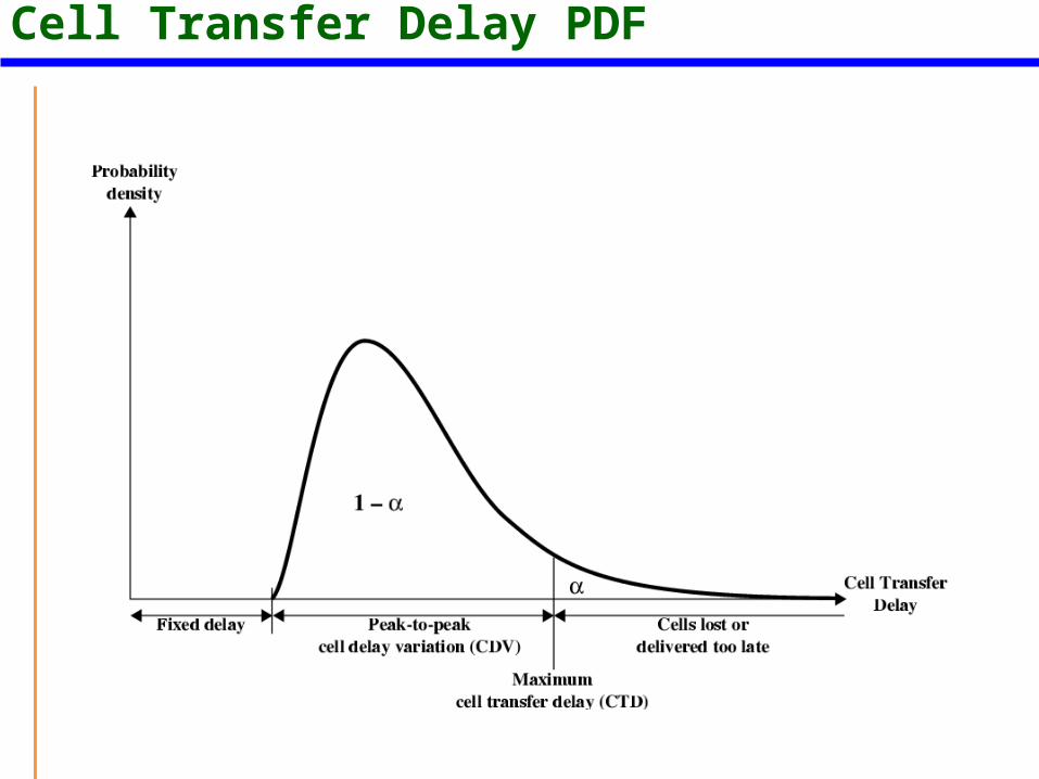
Cell Transfer Delay PDF

Congestion Control Attributes

Only feedback is definedABR and GFRActions taken by network and end systems to regulate traffic submitted

ABR flow controlAdaptively share available bandwidth

Other AttributesBehaviour class selector (BCS)

Support for IP differentiated services (chapter 16)Provides different service levels among UBR connectionsAssociate each connection with a behaviour classMay include queuing and scheduling

Minimum desired cell rate

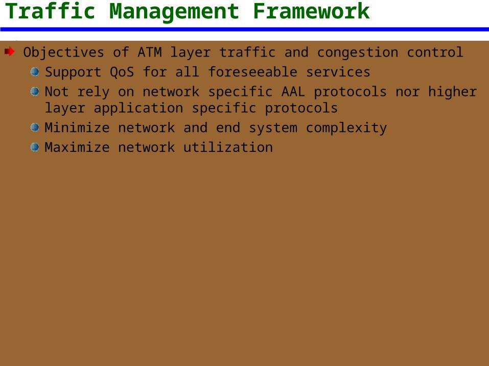
Traffic Management Framework

Objectives of ATM layer traffic and congestion controlSupport QoS for all foreseeable servicesNot rely on network specific AAL protocols nor higher layer application specific protocolsMinimize network and end system complexityMaximize network utilization

Timing Levels

Cell insertion timeRound trip propagation timeConnection durationLong term

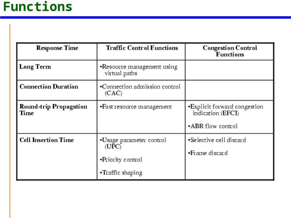
Traffic Control and Congestion Functions

Traffic Control StrategyDetermine whether new ATM connection can be accommodatedAgree performance parameters with subscriberTraffic contract between subscriber and networkThis is congestion avoidance If it fails congestion may occur

Invoke congestion control

Traffic Control

Resource management using virtual pathsConnection admission controlUsage parameter controlSelective cell discardTraffic shapingExplicit forward congestion indication

Resource Management Using Virtual Paths

Allocate resources so that traffic is separated according to service characteristicsVirtual path connection (VPC) are groupings of virtual channel connections (VCC)

ApplicationsUser-to-user applications

VPC between UNI pairNo knowledge of QoS for individual VCCUser checks that VPC can take VCCs’ demands

User-to-network applicationsVPC between UNI and network nodeNetwork aware of and accommodates QoS of VCCs

Network-to-network applicationsVPC between two network nodesNetwork aware of and accommodates QoS of VCCs

Resource Management ConcernsCell loss ratioMax cell transfer delayPeak to peak cell delay variationAll affected by resources devoted to VPCIf VCC goes through multiple VPCs, performance depends on consecutive VPCs and on node performance

VPC performance depends on capacity of VPC and traffic characteristics of VCCsVCC related function depends on switching/processing speed and priority

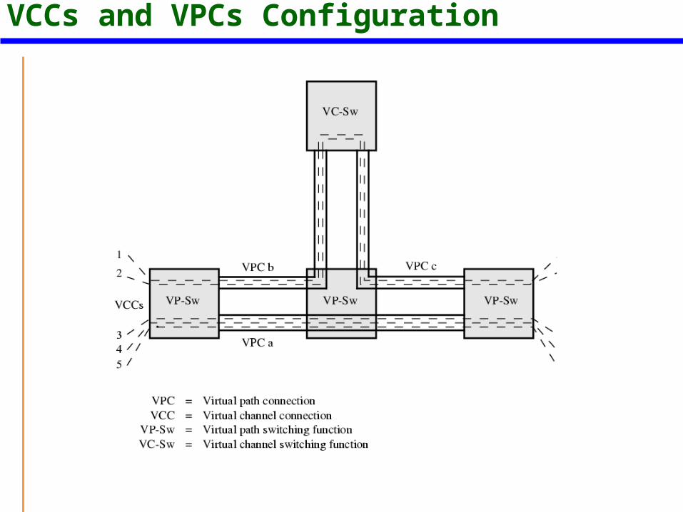
VCCs and VPCs Configuration

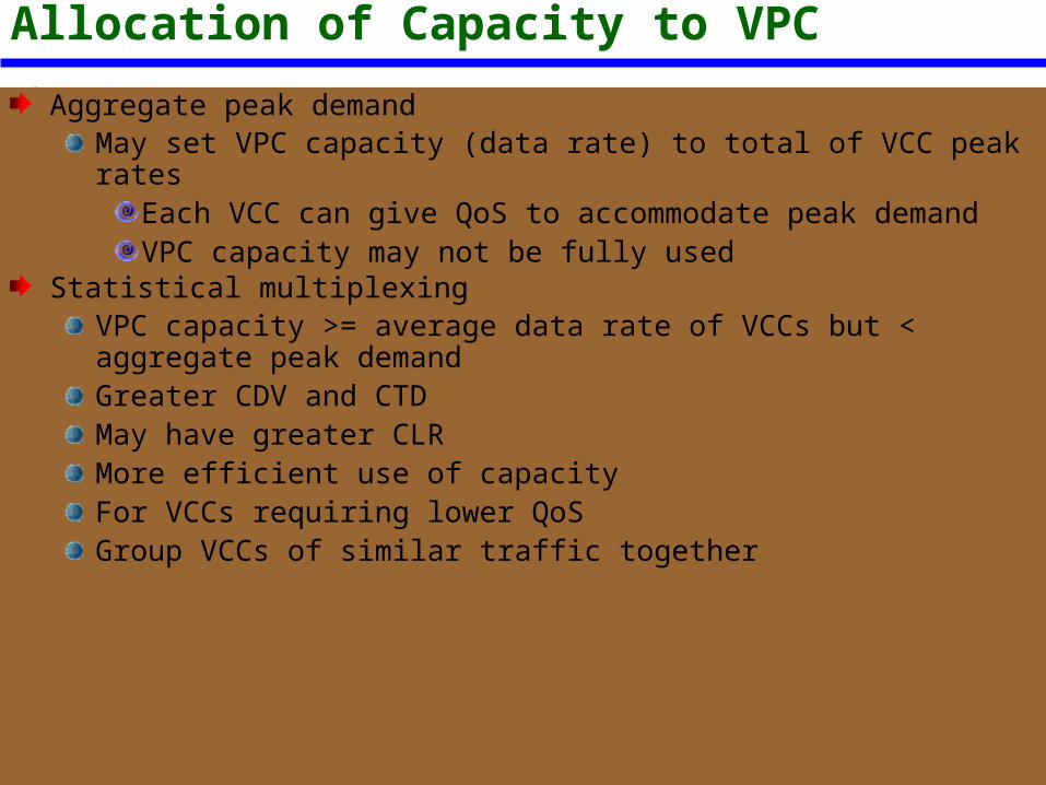
Allocation of Capacity to VPCAggregate peak demand

May set VPC capacity (data rate) to total of VCC peak ratesEach VCC can give QoS to accommodate peak demandVPC capacity may not be fully used

Statistical multiplexingVPC capacity >= average data rate of VCCs but < aggregate peak demandGreater CDV and CTDMay have greater CLRMore efficient use of capacityFor VCCs requiring lower QoSGroup VCCs of similar traffic together

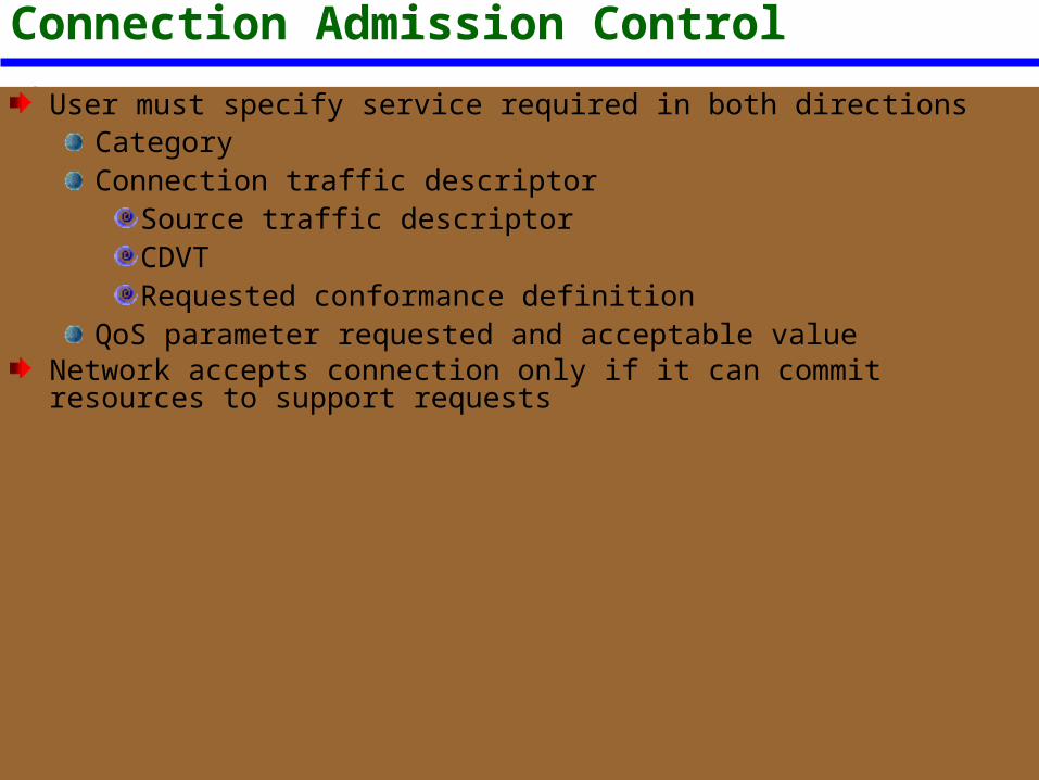
Connection Admission ControlUser must specify service required in both directions

CategoryConnection traffic descriptor

Source traffic descriptorCDVTRequested conformance definition

QoS parameter requested and acceptable valueNetwork accepts connection only if it can commit resources to support requests

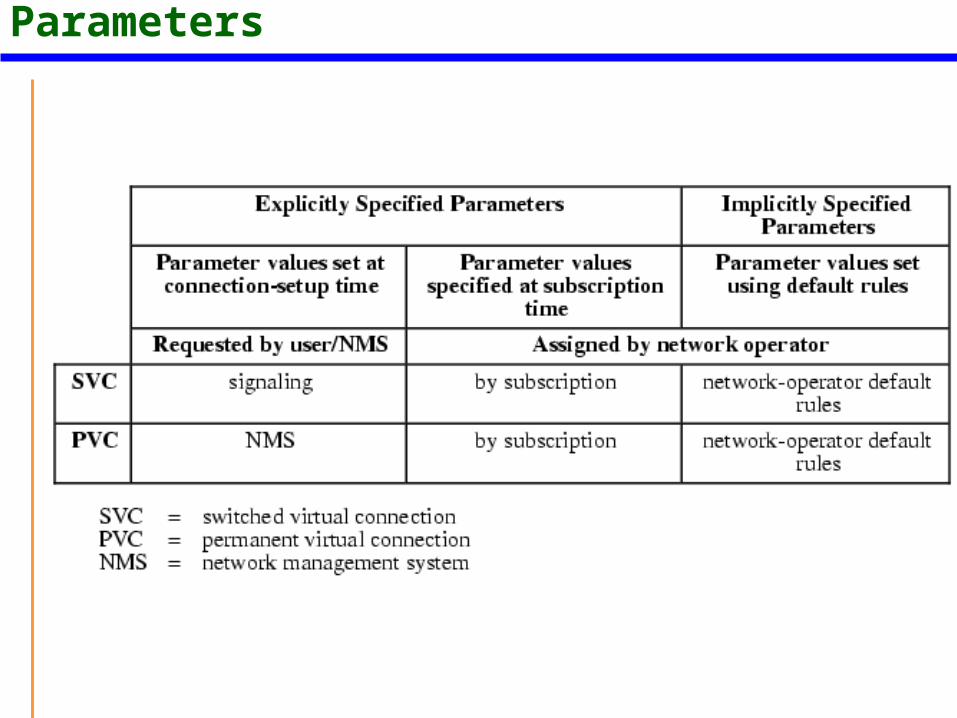
Procedures to Set Traffic Control Parameters

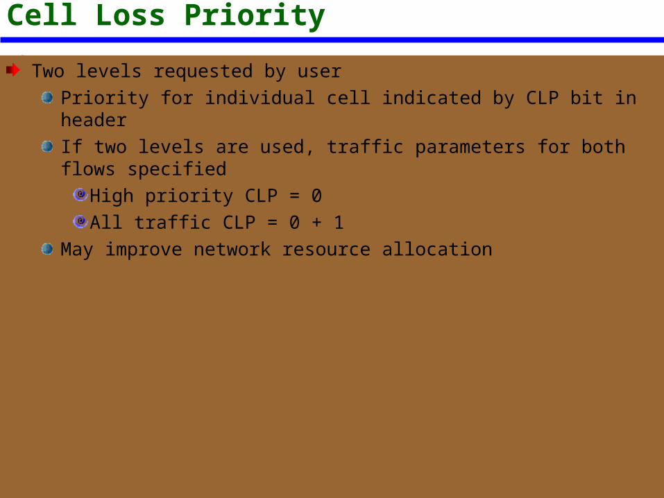
Cell Loss Priority

Two levels requested by userPriority for individual cell indicated by CLP bit in headerIf two levels are used, traffic parameters for both flows specified

High priority CLP = 0All traffic CLP = 0 + 1

May improve network resource allocation

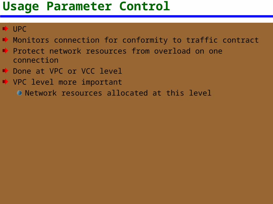
Usage Parameter Control

UPCMonitors connection for conformity to traffic contractProtect network resources from overload on one connectionDone at VPC or VCC levelVPC level more important

Network resources allocated at this level

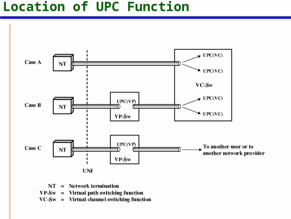
Location of UPC Function

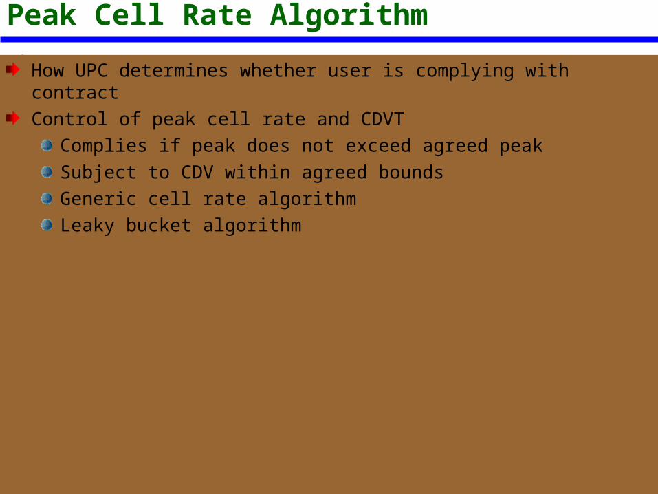
Peak Cell Rate Algorithm

How UPC determines whether user is complying with contractControl of peak cell rate and CDVT

Complies if peak does not exceed agreed peakSubject to CDV within agreed boundsGeneric cell rate algorithmLeaky bucket algorithm

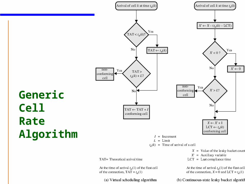
Generic Cell Rate Algorithm

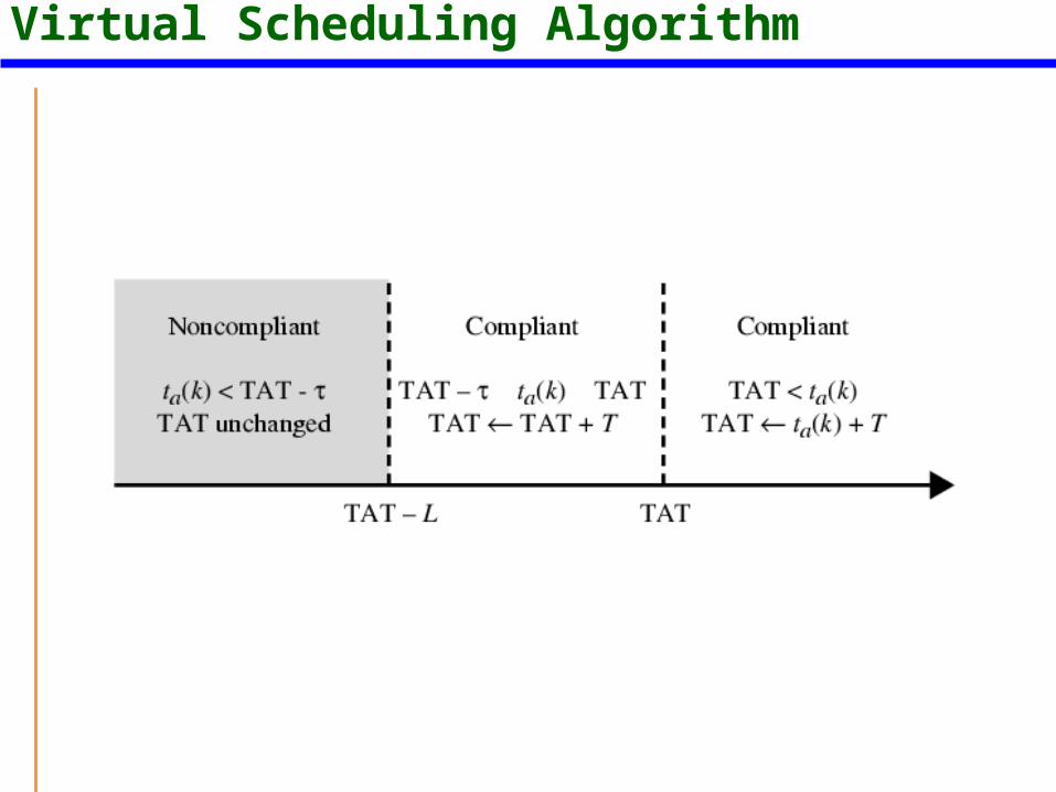
Virtual Scheduling Algorithm

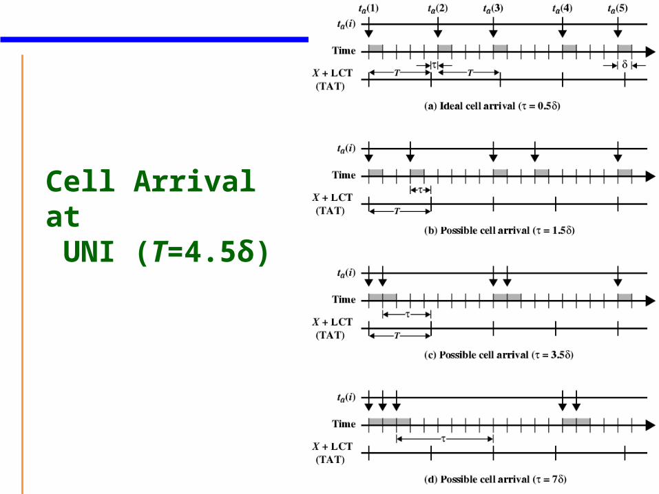
Cell Arrival at UNI (T=4.5δ)

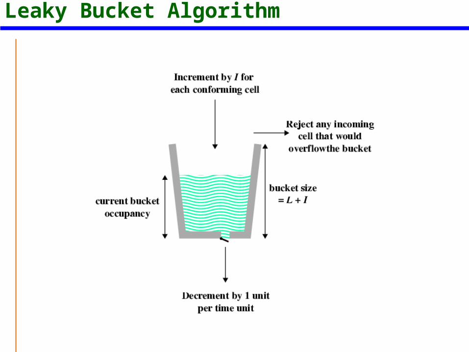
Leaky Bucket Algorithm

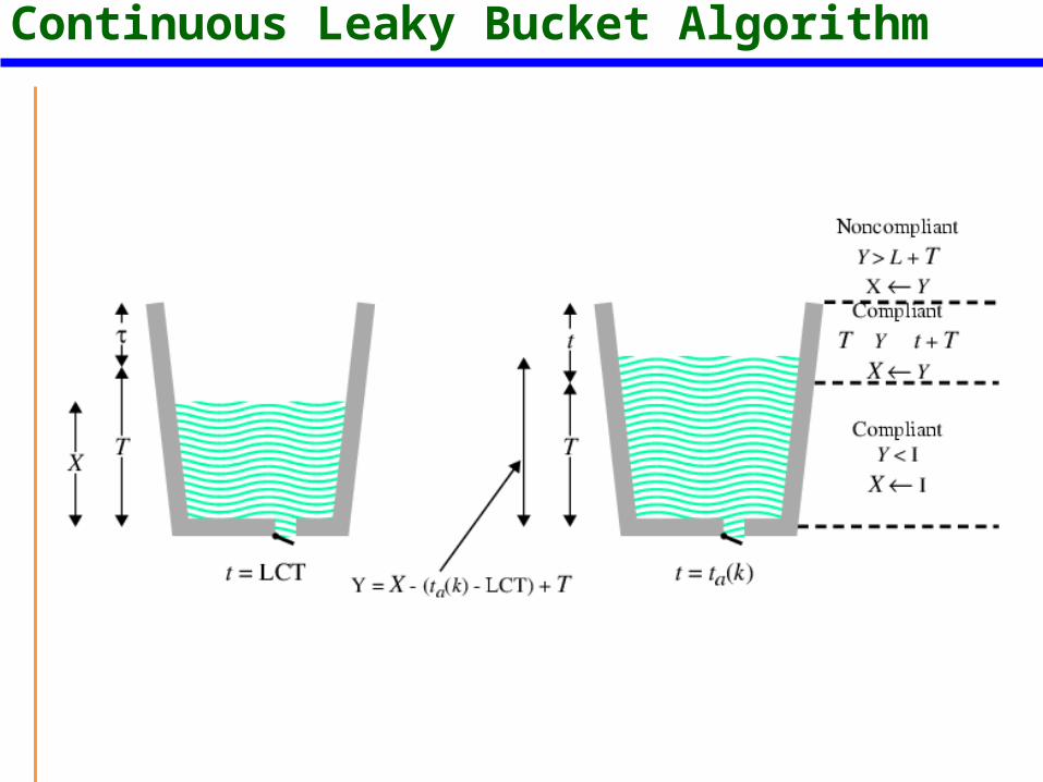
Continuous Leaky Bucket Algorithm

Sustainable Cell Rate Algorithm

Operational definition of relationship between sustainable cell rate and burst toleranceUsed by UPC to monitor complianceSame algorithm as peak cell rate

UPC Actions

Compliant cell pass, non-compliant cells discardedIf no additional resources allocated to CLP=1 traffic, CLP=0 cells CIf two level cell loss priority cell with:

CLP=0 and conforms passesCLP=0 non-compliant for CLP=0 traffic but compliant for CLP=0+1 is tagged and passesCLP=0 non-compliant for CLP=0 and CLP=0+1 traffic discardedCLP=1 compliant for CLP=0+1 passesCLP=1 non-compliant for CLP=0+1 discarded

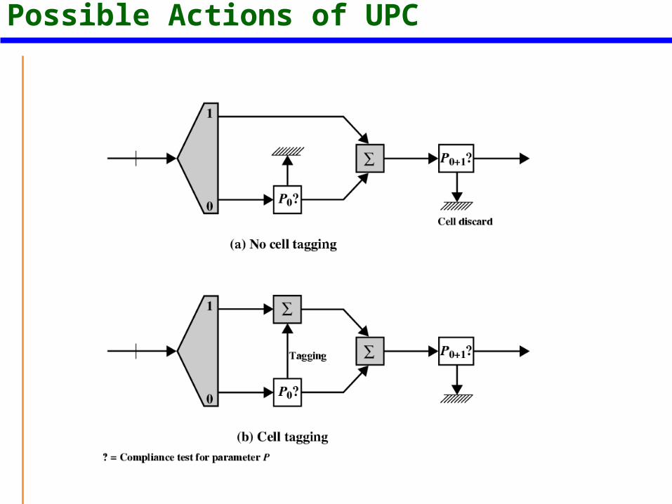
Possible Actions of UPC

Selective Cell Discard

Starts when network, at point beyond UPC, discards CLP=1 cellsDiscard low priority cells to protect high priority cellsNo distinction between cells labelled low priority by source and those tagged by UPC

Traffic Shaping

GCRA is a form of traffic policingFlow of cells regulatedCells exceeding performance level tagged or discarded

Traffic shaping used to smooth traffic flowReduce cell clumpingFairer allocation of resourcesReduced average delay

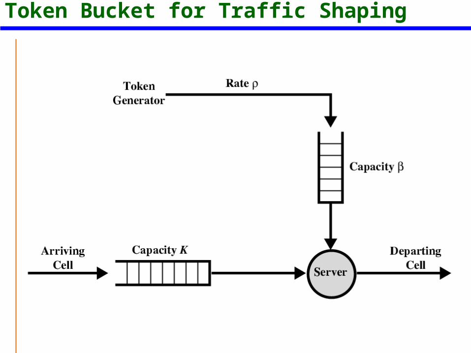
Token Bucket for Traffic Shaping

Explicit Forward Congestion Indication

Essentially same as frame relayIf node experiencing congestion, set forward congestion indication is cell headers

Tells users that congestion avoidance should be initiated in this directionUser may take action at higher level

ABR Traffic ManagementQoS for CBR, VBR based on traffic contract and UPC described previouslyNo congestion feedback to sourceOpen-loop controlNot suited to non-real-time applications

File transfer, web access, RPC, distributed file systemsNo well defined traffic characteristics except PCRPCR not enough to allocate resources

Use best efforts or closed-loop control

Best Efforts

Share unused capacity between applicationsAs congestion goes up:

Cells are lostSources back off and reduce rateFits well with TCP techniques (chapter 12)Inefficient

Cells dropped causing re-transmission

Closed-Loop Control

Sources share capacity not used by CBR and VBRProvide feedback to sources to adjust loadAvoid cell lossShare capacity fairlyUsed for ABR

Characteristics of ABRABR connections share available capacity

Access instantaneous capacity unused by CBR/VBRIncreases utilization without affecting CBR/VBR QoS

Share used by single ABR connection is dynamicVaries between agreed MCR and PCR

Network gives feedback to ABR sourcesABR flow limited to available capacityBuffers absorb excess traffic prior to arrival of feedback

Low cell lossMajor distinction from UBR

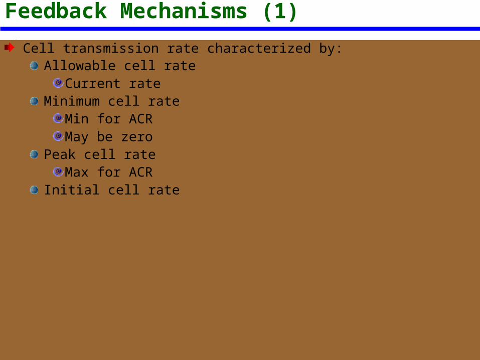
Feedback Mechanisms (1)Cell transmission rate characterized by:

Allowable cell rateCurrent rate

Minimum cell rateMin for ACRMay be zero

Peak cell rateMax for ACR

Initial cell rate

Feedback Mechanisms (2)

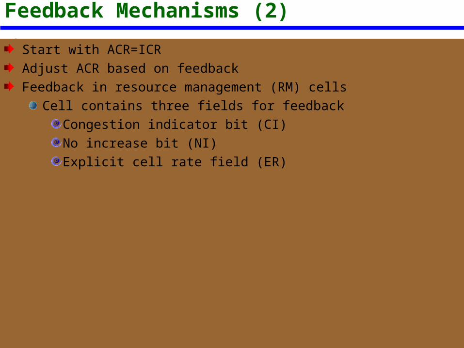
Start with ACR=ICRAdjust ACR based on feedbackFeedback in resource management (RM) cells

Cell contains three fields for feedbackCongestion indicator bit (CI)No increase bit (NI)Explicit cell rate field (ER)

Source Reaction to Feedback

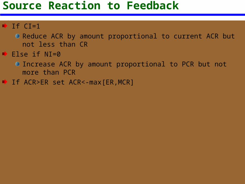
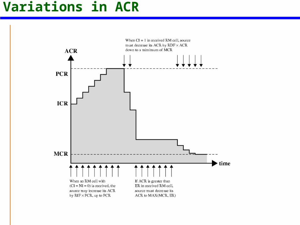
If CI=1Reduce ACR by amount proportional to current ACR but not less than CR

Else if NI=0Increase ACR by amount proportional to PCR but not more than PCR

If ACR>ER set ACR<-max[ER,MCR]

Variations in ACR

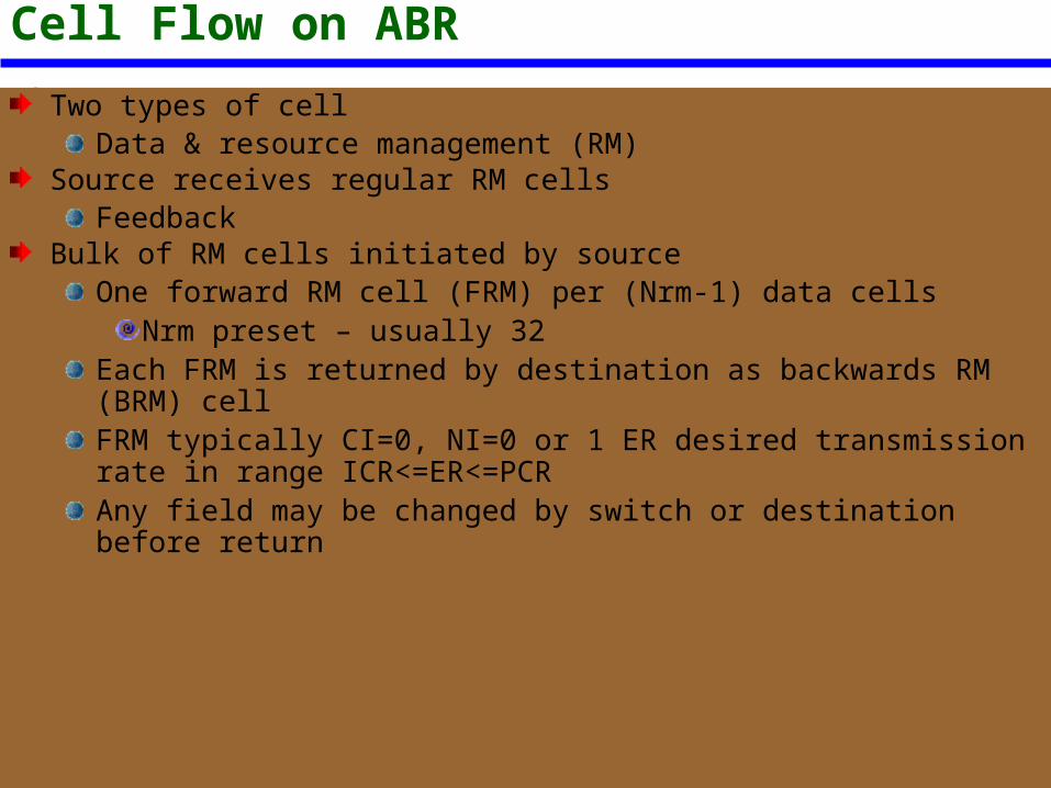
Cell Flow on ABRTwo types of cell

Data & resource management (RM)Source receives regular RM cells

FeedbackBulk of RM cells initiated by source

One forward RM cell (FRM) per (Nrm-1) data cellsNrm preset – usually 32

Each FRM is returned by destination as backwards RM (BRM) cellFRM typically CI=0, NI=0 or 1 ER desired transmission rate in range ICR<=ER<=PCRAny field may be changed by switch or destination before return

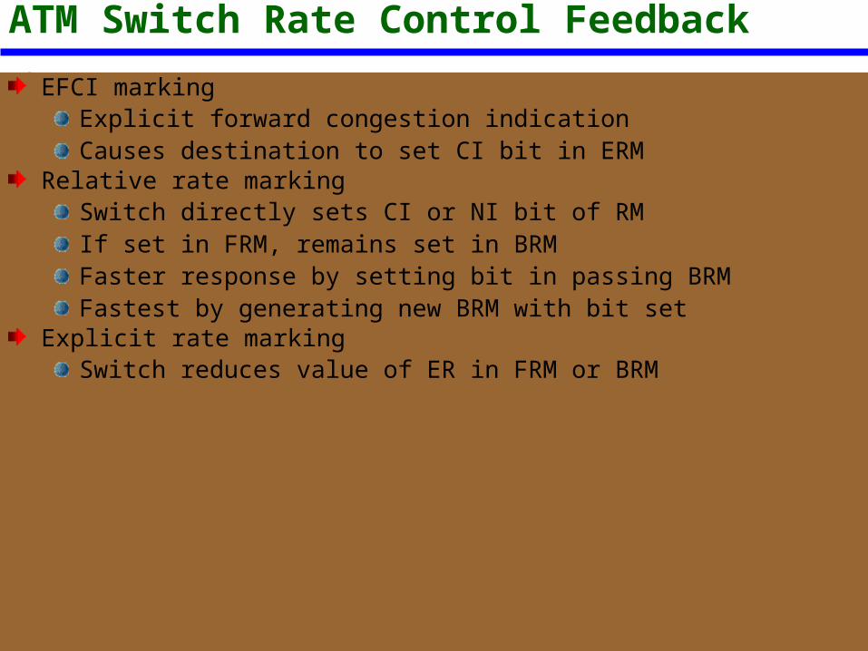
ATM Switch Rate Control FeedbackEFCI marking

Explicit forward congestion indicationCauses destination to set CI bit in ERM

Relative rate markingSwitch directly sets CI or NI bit of RMIf set in FRM, remains set in BRMFaster response by setting bit in passing BRMFastest by generating new BRM with bit set

Explicit rate markingSwitch reduces value of ER in FRM or BRM

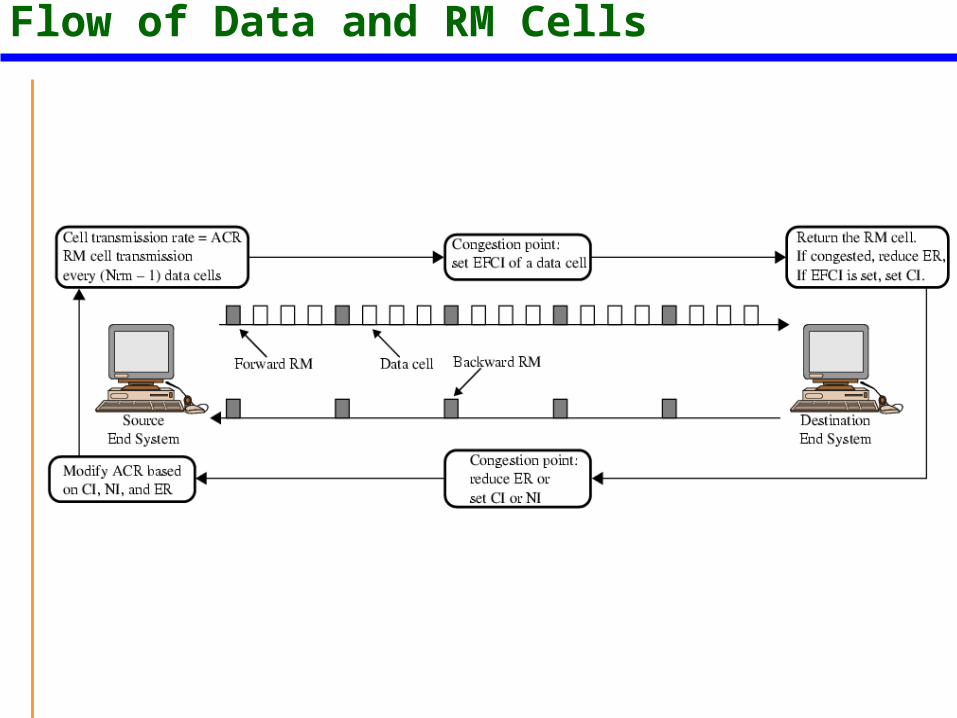
Flow of Data and RM Cells

ARB Feedback v TCP ACK

ABR feedback controls rate of transmissionRate control

TCP feedback controls window sizeCredit control

ARB feedback from switches or destinationTCP feedback from destination only

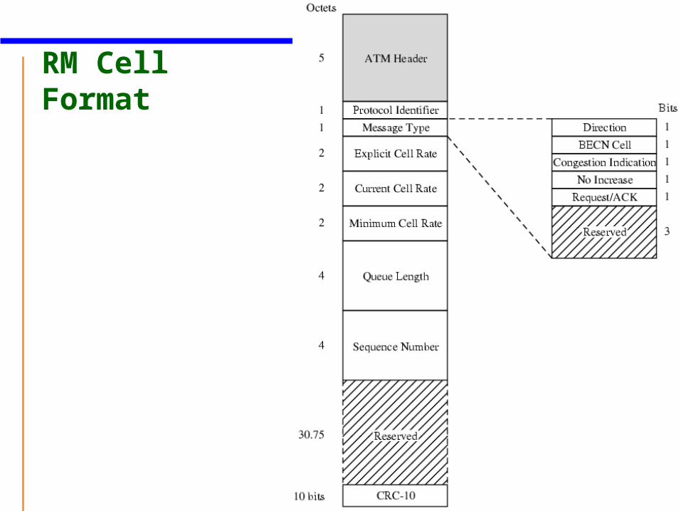
RM Cell Format

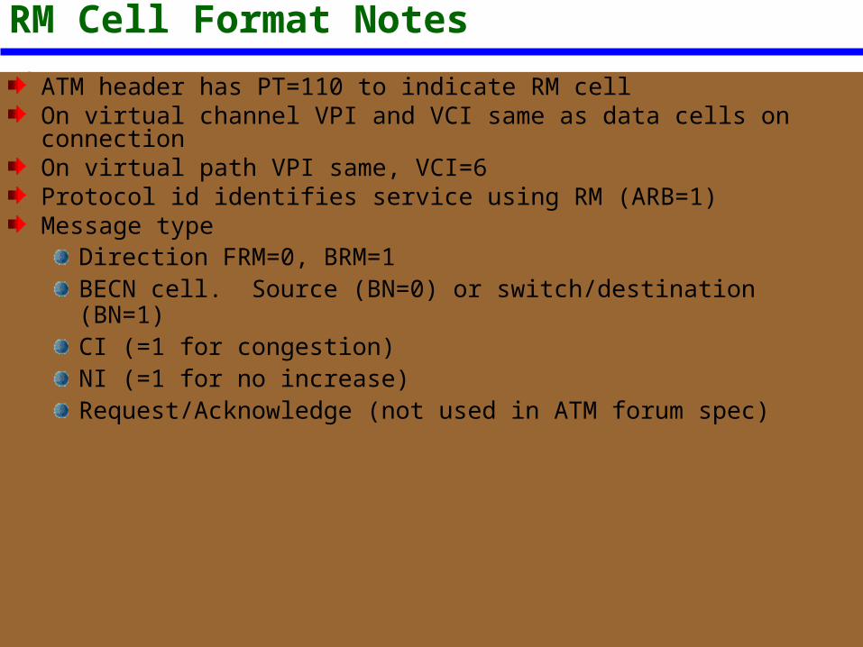
RM Cell Format NotesATM header has PT=110 to indicate RM cellOn virtual channel VPI and VCI same as data cells on connectionOn virtual path VPI same, VCI=6Protocol id identifies service using RM (ARB=1)Message type

Direction FRM=0, BRM=1BECN cell. Source (BN=0) or switch/destination (BN=1)CI (=1 for congestion)NI (=1 for no increase)Request/Acknowledge (not used in ATM forum spec)

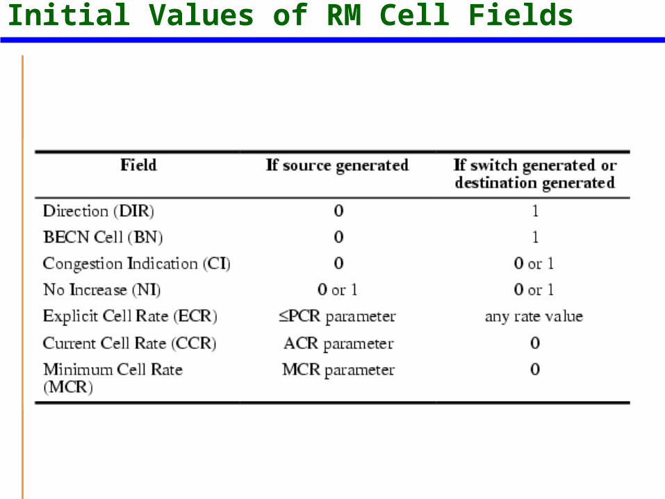
Initial Values of RM Cell Fields

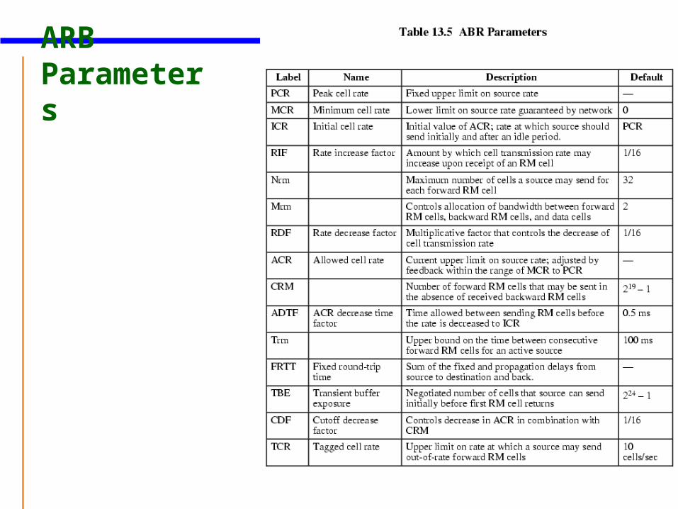
ARB Parameters

ARB Capacity AllocationATM switch must perform:

Congestion controlMonitor queue length

Fair capacity allocationThrottle back connections using more than fair share

ATM rate control signals are explicitTCP are implicit

Increasing delay and cell loss

Congestion Control Algorithms- Binary Feedback

Use only EFCI, CI and NI bitsSwitch monitors buffer utilizationWhen congestion approaches, binary notification

Set EFCI on forward data cells or CI or NI on FRM or BRMThree approaches to which to notify

Single FIFO queueMultiple queuesFair share notification

Single FIFO Queue

When buffer use exceeds threshold (e.g. 80%)Switch starts issuing binary notificationsContinues until buffer use falls below thresholdCan have two thresholds

One for start and one for stopStops continuous on/off switching

Biased against connections passing through more switches

Multiple Queues

Separate queue for each VC or group of VCsSeparate threshold on each queueOnly connections with long queues get binary notifications

FairBadly behaved source does not affect other VCsDelay and loss behaviour of individual VCs separated

Can have different QoS on different VCs

Fair Share

Selective feedback or intelligent markingTry to allocate capacity dynamically E.g. fairshare =(target rate)/(number of connections)Mark any cells where CCR>fairshare

Explicit Rate Feedback SchemesCompute fair share of capacity for each VCDetermine current load or congestionCompute explicit rate (ER) for each connection and send to sourceThree algorithms

Enhanced proportional rate control algorithmEPRCA

Explicit rate indication for congestion avoidanceERICA

Congestion avoidance using proportional controlCAPC

Enhanced Proportional Rate Control Algorithm(EPRCA)

Switch tracks average value of current load on each connectionMean allowed cell rate (MARC)MACR(I)=(1-α)*(MACR(I-1) + α*CCR(I)CCR(I) is CCR field in Ith FRMTypically α=1/16Bias to past values of CCR over currentGives estimated average load passing through switchIf congestion, switch reduces each VC to no more than DPF*MACR

DPF=down pressure factor, typically 7/8ER<-min[ER, DPF*MACR]

Load Factor

Adjustments based on load factor LF=Input rate/target rate

Input rate measured over fixed averaging intervalTarget rate slightly below link bandwidth (85 to 90%)LF>1 congestion threatened

VCs will have to reduce rate

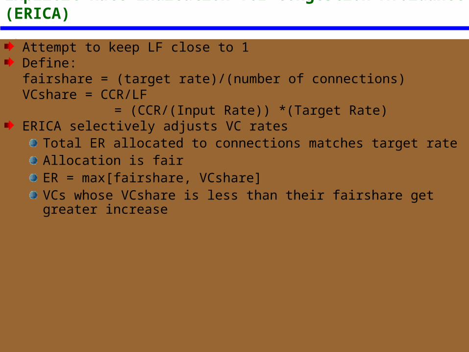
Explicit Rate Indication for Congestion Avoidance (ERICA)

Attempt to keep LF close to 1Define:fairshare = (target rate)/(number of connections)VCshare = CCR/LF

= (CCR/(Input Rate)) *(Target Rate)ERICA selectively adjusts VC rates

Total ER allocated to connections matches target rateAllocation is fairER = max[fairshare, VCshare]VCs whose VCshare is less than their fairshare get greater increase

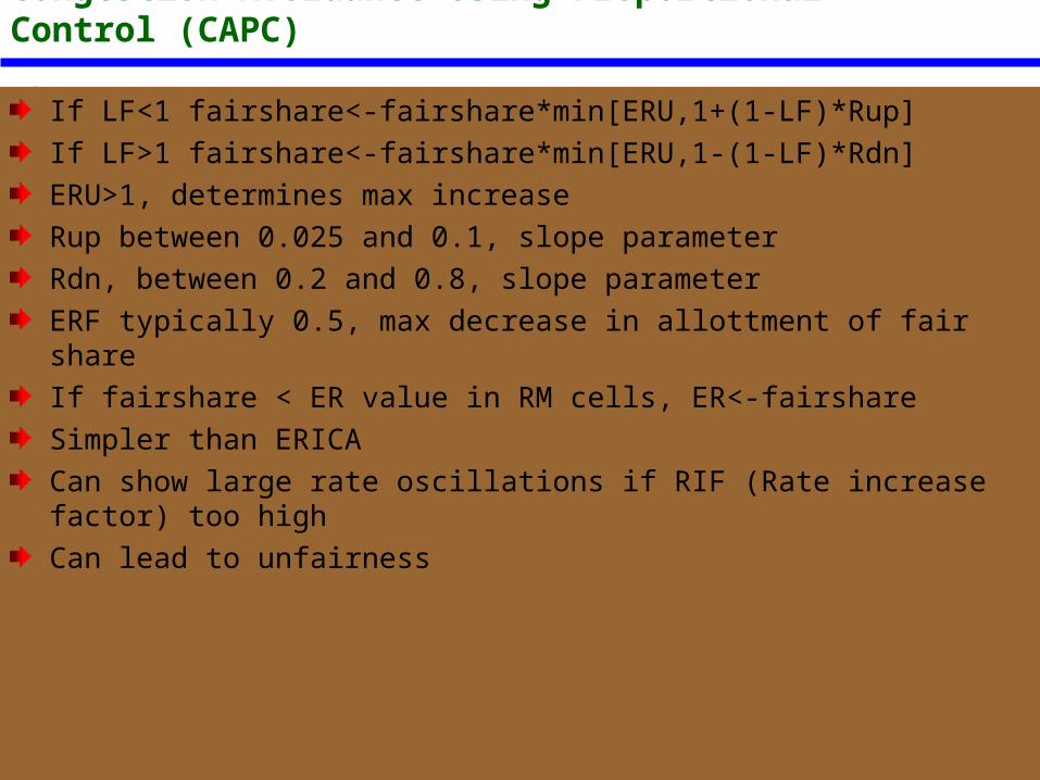
Congestion Avoidance Using Proportional Control (CAPC)

If LF<1 fairshare<-fairshare*min[ERU,1+(1-LF)*Rup]If LF>1 fairshare<-fairshare*min[ERU,1-(1-LF)*Rdn]ERU>1, determines max increaseRup between 0.025 and 0.1, slope parameterRdn, between 0.2 and 0.8, slope parameterERF typically 0.5, max decrease in allottment of fair shareIf fairshare < ER value in RM cells, ER<-fairshareSimpler than ERICACan show large rate oscillations if RIF (Rate increase factor) too highCan lead to unfairness

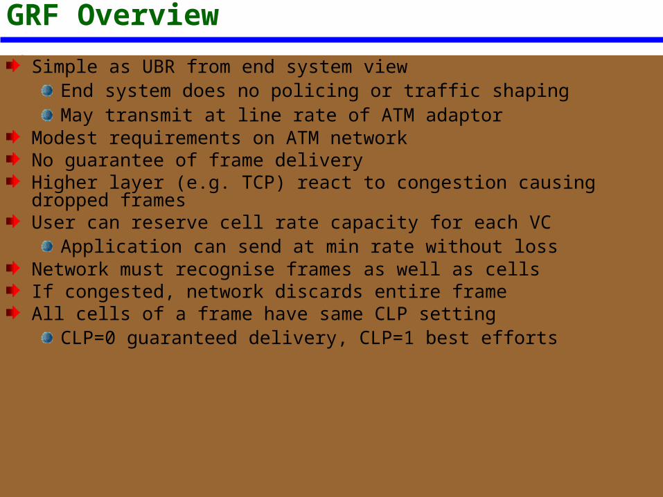
GRF OverviewSimple as UBR from end system view

End system does no policing or traffic shapingMay transmit at line rate of ATM adaptor

Modest requirements on ATM networkNo guarantee of frame deliveryHigher layer (e.g. TCP) react to congestion causing dropped framesUser can reserve cell rate capacity for each VC

Application can send at min rate without lossNetwork must recognise frames as well as cellsIf congested, network discards entire frameAll cells of a frame have same CLP setting

CLP=0 guaranteed delivery, CLP=1 best efforts

GFR Traffic Contract

Peak cell rate PCRMinimum cell rate MCRMaximum burst size MBSMaximum frame size MFSCell delay variation tolerance CDVT

Mechanisms for supporting Rate Guarantees

Tagging and policingBuffer managementScheduling

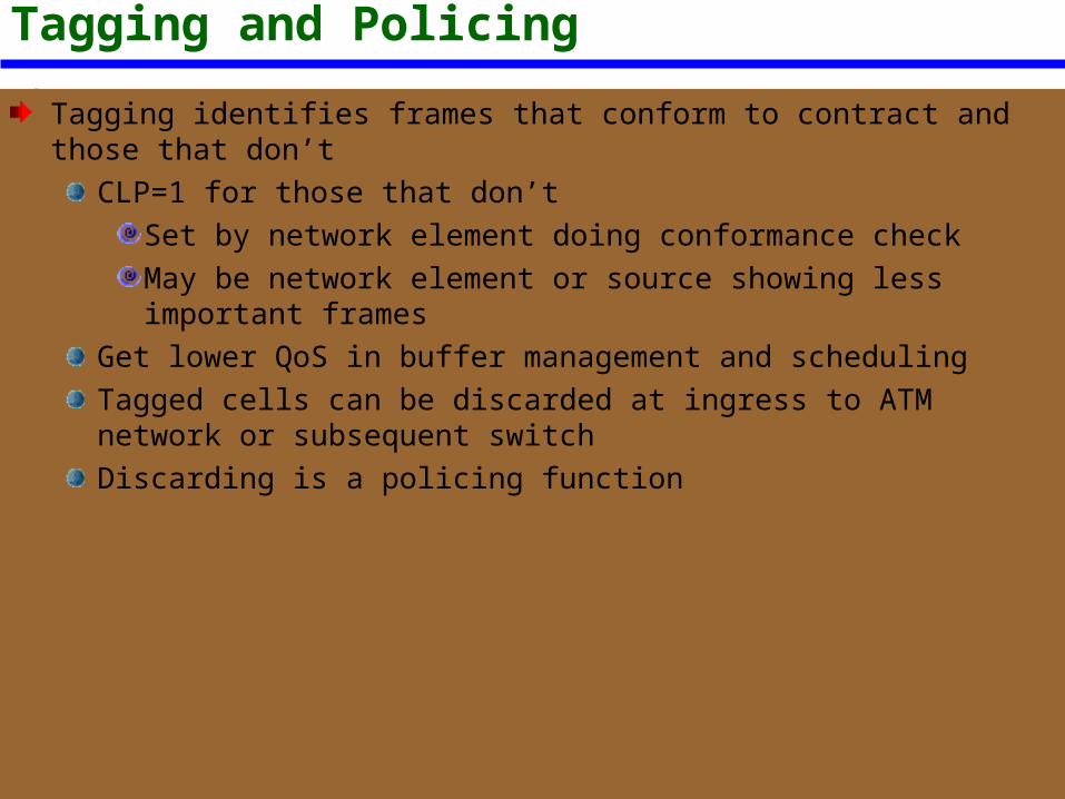
Tagging and Policing

Tagging identifies frames that conform to contract and those that don’tCLP=1 for those that don’t

Set by network element doing conformance checkMay be network element or source showing less important frames

Get lower QoS in buffer management and schedulingTagged cells can be discarded at ingress to ATM network or subsequent switchDiscarding is a policing function

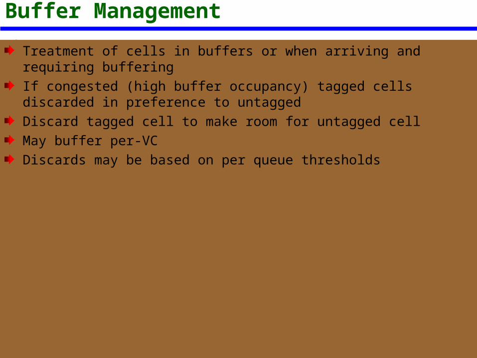
Buffer Management

Treatment of cells in buffers or when arriving and requiring bufferingIf congested (high buffer occupancy) tagged cells discarded in preference to untaggedDiscard tagged cell to make room for untagged cellMay buffer per-VCDiscards may be based on per queue thresholds

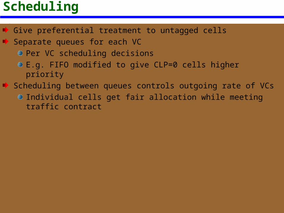
Scheduling

Give preferential treatment to untagged cellsSeparate queues for each VC

Per VC scheduling decisionsE.g. FIFO modified to give CLP=0 cells higher priority

Scheduling between queues controls outgoing rate of VCsIndividual cells get fair allocation while meeting traffic contract

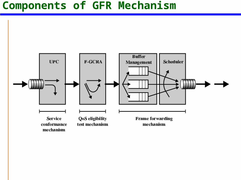
Components of GFR Mechanism

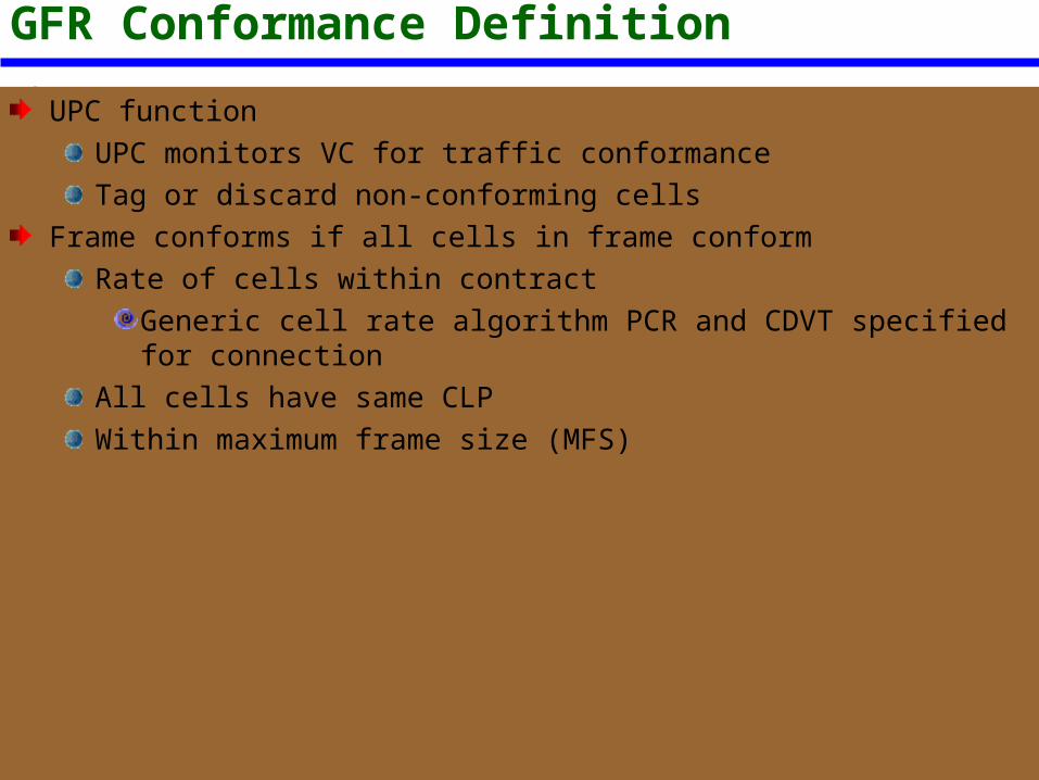
GFR Conformance Definition

UPC functionUPC monitors VC for traffic conformance Tag or discard non-conforming cells

Frame conforms if all cells in frame conformRate of cells within contract

Generic cell rate algorithm PCR and CDVT specified for connectionAll cells have same CLPWithin maximum frame size (MFS)

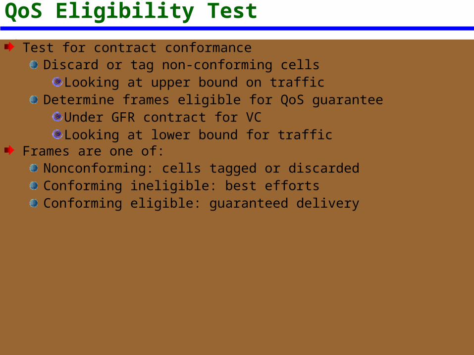
QoS Eligibility TestTest for contract conformance

Discard or tag non-conforming cellsLooking at upper bound on traffic

Determine frames eligible for QoS guaranteeUnder GFR contract for VCLooking at lower bound for traffic

Frames are one of:Nonconforming: cells tagged or discardedConforming ineligible: best effortsConforming eligible: guaranteed delivery

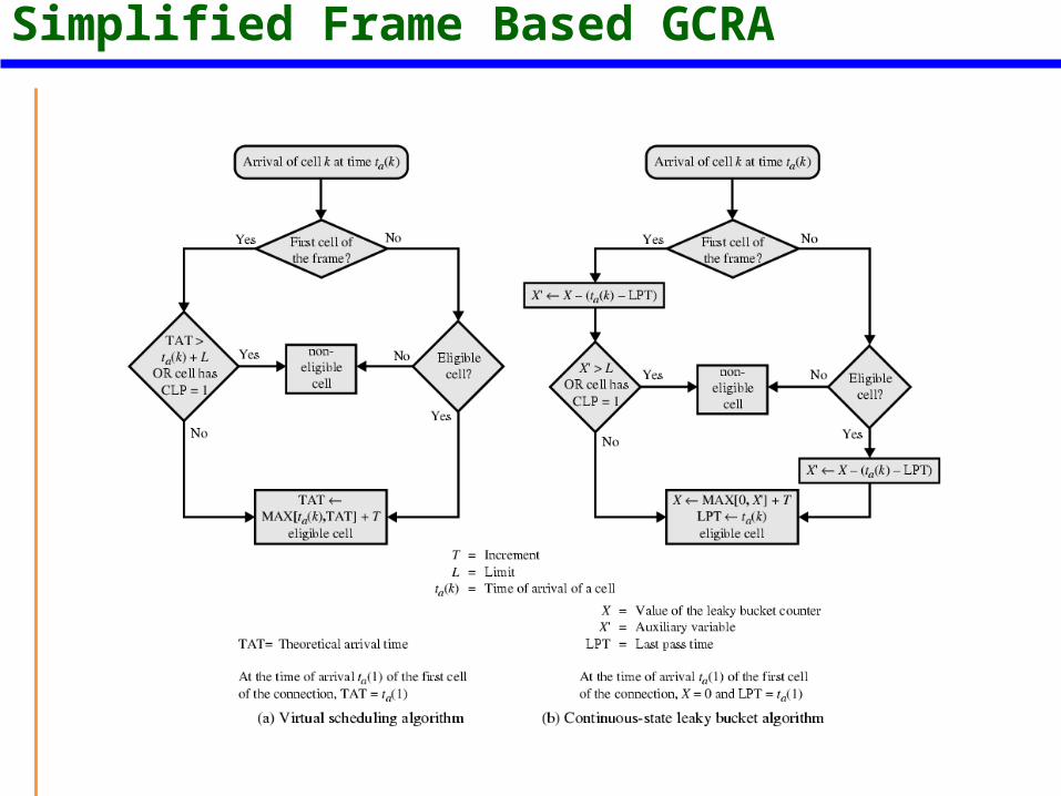
Simplified Frame Based GCRA

ATM Traffic Management

Section 13.6 will be skipped except for the following

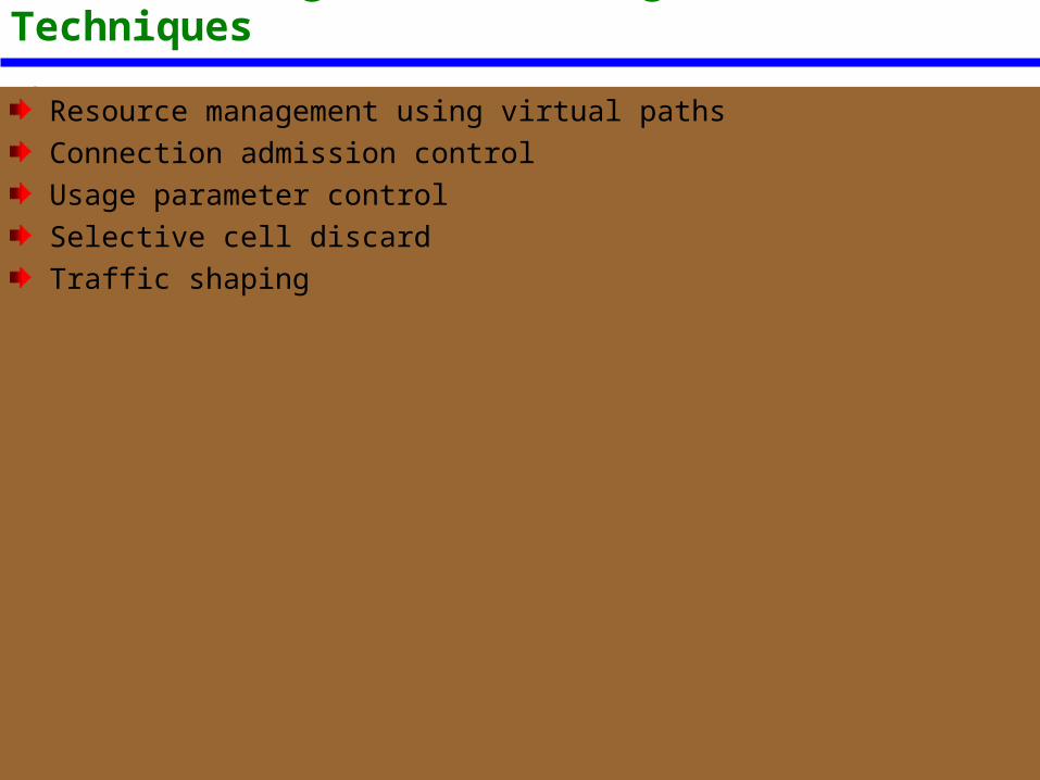
Traffic Management and Congestion Control Techniques

Resource management using virtual pathsConnection admission controlUsage parameter controlSelective cell discardTraffic shaping

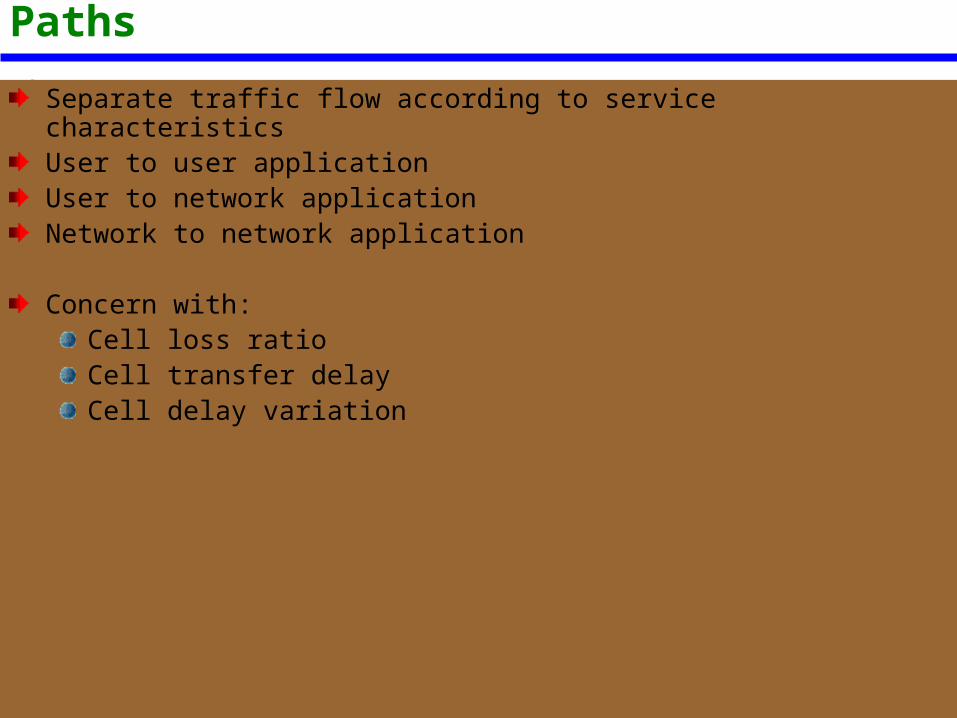
Resource Management Using Virtual Paths

Separate traffic flow according to service characteristicsUser to user applicationUser to network applicationNetwork to network application

Concern with:Cell loss ratioCell transfer delayCell delay variation

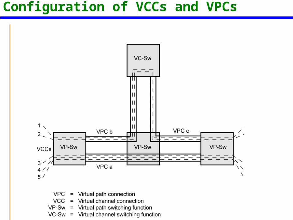
Configuration of VCCs and VPCs

Allocating VCCs within VPC

All VCCs within VPC should experience similar network performanceOptions for allocation:

Aggregate peak demandStatistical multiplexing

Connection Admission Control

First line of defenseUser specifies traffic characteristics for new connection (VCC or VPC) by selecting a QoSNetwork accepts connection only if it can meet the demandTraffic contract

Peak cell rateCell delay variationSustainable cell rateBurst tolerance

Usage Parameter Control

Monitor connection to ensure traffic conforms to contractProtection of network resources from overload by one connectionDone on VCC and VPCPeak cell rate and cell delay variationSustainable cell rate and burst toleranceDiscard cells that do not conform to traffic contractCalled traffic policing

Traffic Shaping

Smooth out traffic flow and reduce cell clumpingToken bucket

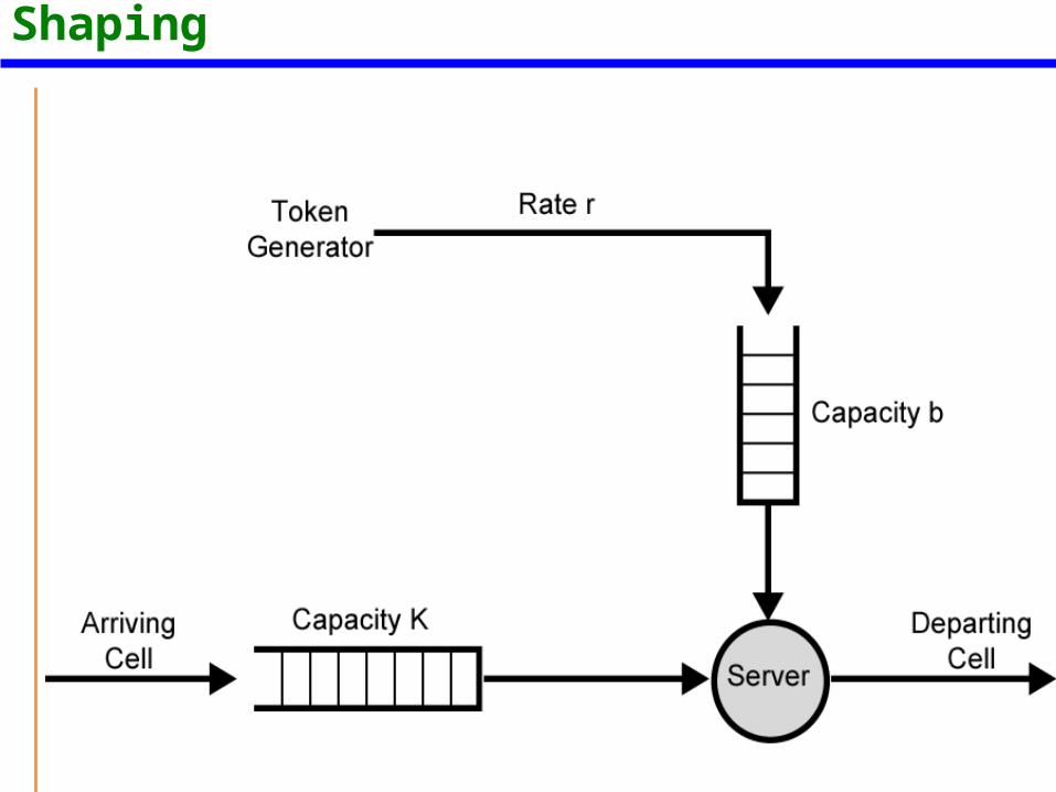
Token Bucket for Traffic Shaping

UNIT IVIntegrated and Differentiated Services

IntroductionNew additions to Internet increasing traffic

High volume client/server applicationWeb

GraphicsReal time voice and video

Need to manage traffic and control congestionIEFT standards

Integrated servicesCollective service to set of traffic demands in domain

– Limit demand & reserve resourcesDifferentiated services

Classify traffic in groupsDifferent group traffic handled differently

Integrated Services Architecture (ISA)

IPv4 header fields for precedence and type of service usually ignoredATM only network designed to support TCP, UDP and real-time traffic

May need new installationNeed to support Quality of Service (QoS) within TCP/IP

Add functionality to routersMeans of requesting QoS

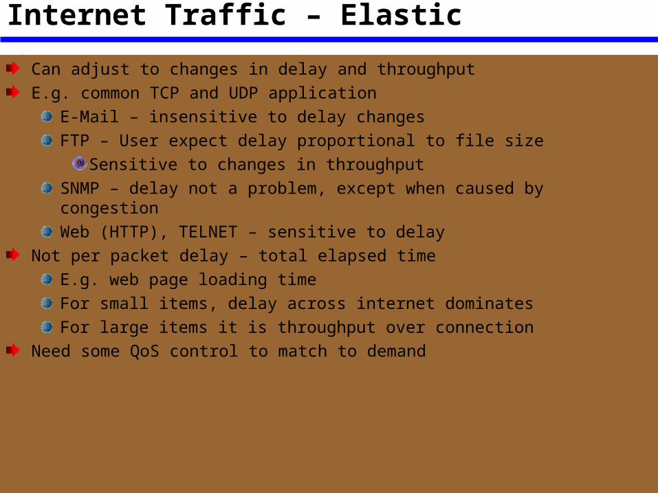
Internet Traffic – Elastic

Can adjust to changes in delay and throughputE.g. common TCP and UDP application

E-Mail – insensitive to delay changesFTP – User expect delay proportional to file size

Sensitive to changes in throughputSNMP – delay not a problem, except when caused by congestionWeb (HTTP), TELNET – sensitive to delay

Not per packet delay – total elapsed timeE.g. web page loading timeFor small items, delay across internet dominates For large items it is throughput over connection

Need some QoS control to match to demand

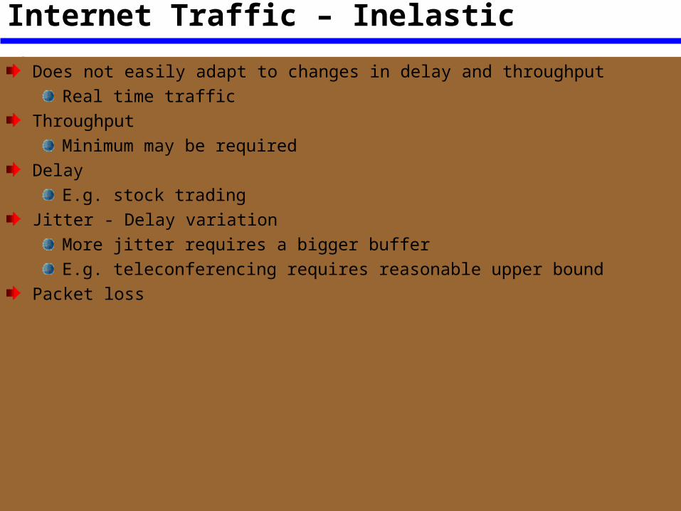
Internet Traffic – Inelastic

Does not easily adapt to changes in delay and throughputReal time traffic

ThroughputMinimum may be required

DelayE.g. stock trading

Jitter - Delay variationMore jitter requires a bigger bufferE.g. teleconferencing requires reasonable upper bound

Packet loss

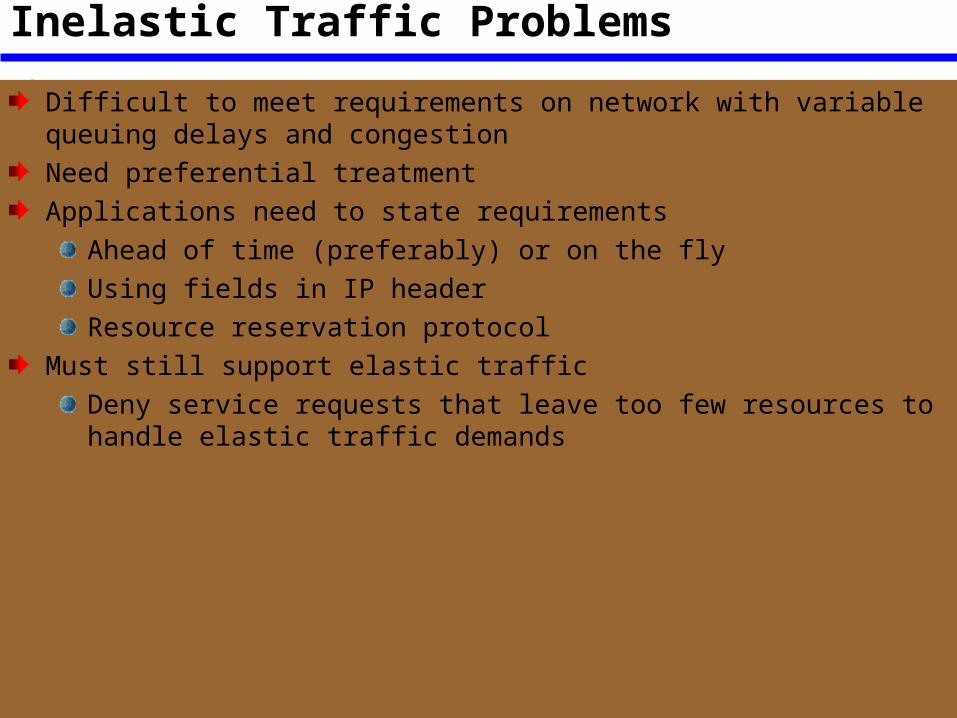
Inelastic Traffic Problems

Difficult to meet requirements on network with variable queuing delays and congestionNeed preferential treatment Applications need to state requirements

Ahead of time (preferably) or on the flyUsing fields in IP headerResource reservation protocol

Must still support elastic trafficDeny service requests that leave too few resources to handle elastic traffic demands

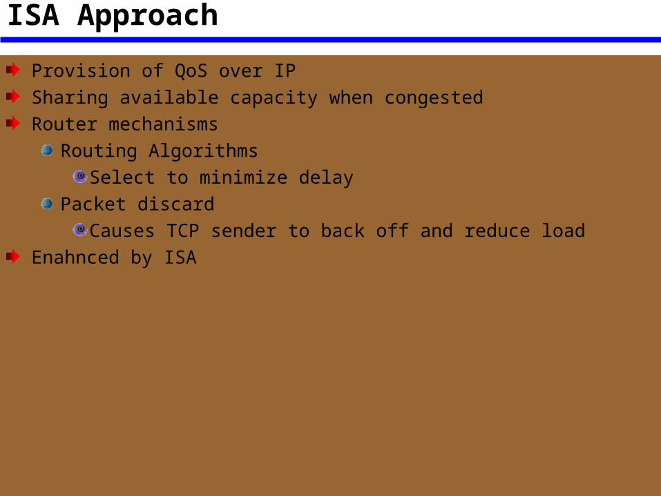
ISA Approach

Provision of QoS over IPSharing available capacity when congestedRouter mechanisms

Routing AlgorithmsSelect to minimize delay

Packet discardCauses TCP sender to back off and reduce load

Enahnced by ISA

Flow

IP packet can be associated with a flowDistinguishable stream of related IP packetsFrom single user activityRequiring same QoSE.g. one transport connection or one video streamUnidirectionalCan be more than one recipient

MulticastMembership of flow identified by source and destination IP address, port numbers, protocol typeIPv6 header flow identifier can be used but isnot necessarily equivalent to ISA flow

ISA Functions

Admission controlFor QoS, reservation required for new flowRSVP used

Routing algorithmBase decision on QoS parameters

Queuing disciplineTake account of different flow requirements

Discard policyManage congestionMeet QoS

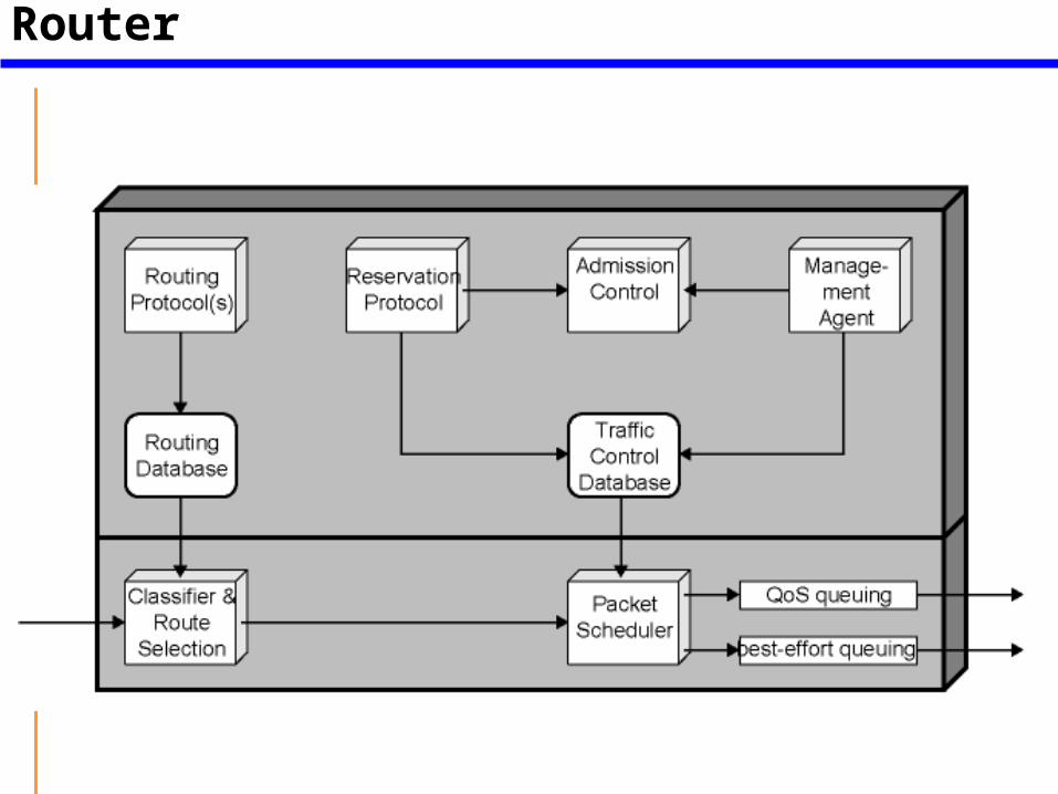
Figure 9.1 ISA Implemented in Router

ISA Components – Background Functions

Reservation ProtocolRSVP

Admission controlManagement agent

Can use agent to modify traffic control database and direct admission controlRouting protocol

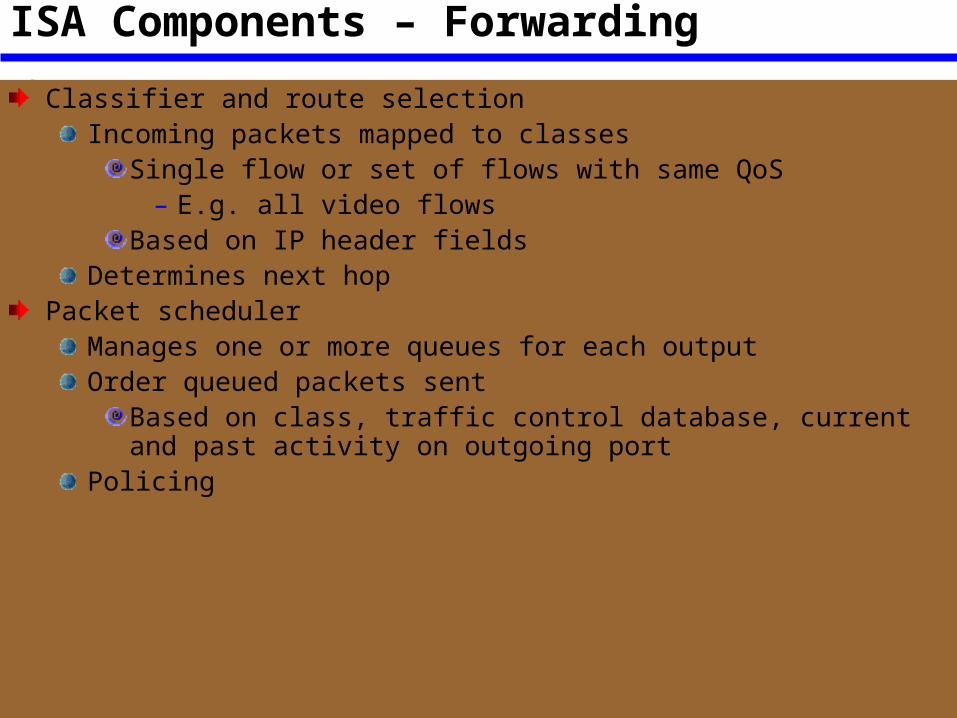
ISA Components – Forwarding

Classifier and route selectionIncoming packets mapped to classes

Single flow or set of flows with same QoS– E.g. all video flows

Based on IP header fieldsDetermines next hop

Packet schedulerManages one or more queues for each outputOrder queued packets sent

Based on class, traffic control database, current and past activity on outgoing port

Policing

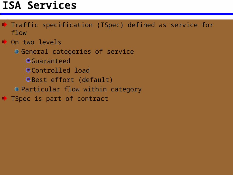
ISA Services

Traffic specification (TSpec) defined as service for flow On two levels

General categories of serviceGuaranteedControlled loadBest effort (default)

Particular flow within categoryTSpec is part of contract

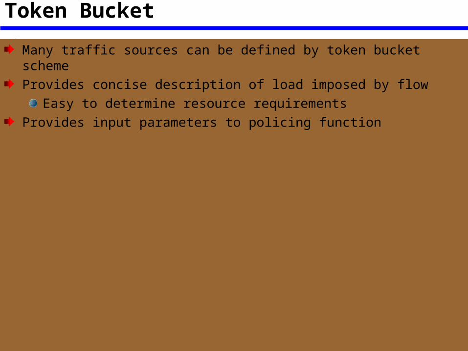
Token Bucket

Many traffic sources can be defined by token bucket schemeProvides concise description of load imposed by flow

Easy to determine resource requirementsProvides input parameters to policing function

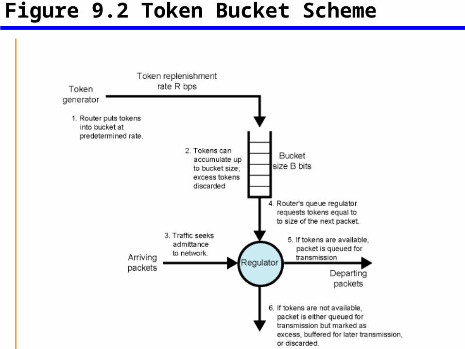
Figure 9.2 Token Bucket Scheme

ISA Services –Guaranteed Service

Assured capacity level or data rateSpecific upper bound on queuing delay through network

Must be added to propagation delay or latency to get total delaySet high to accommodate rare long queue delays

No queuing lossesI.e. no buffer overflow

E.g. Real time play back of incoming signal can use delay buffer for incoming signal but will not tolerate packet loss

ISA Services – Controlled Load

Tightly approximates to best efforts under unloaded conditionsNo upper bound on queuing delay

High percentage of packets do not experience delay over minimum transit delayPropagation plus router processing with no queuing delay

Very high percentage deliveredAlmost no queuing loss

Adaptive real time applicationsReceiver measures jitter and sets playback pointVideo can drop a frame or delay output slightlyVoice can adjust silence periods

Queuing Discipline

Traditionally first in first out (FIFO) or first come first served (FCFS) at each router portNo special treatment to high priority packets (flows)Small packets held up by large packets ahead of them in queue

Larger average delay for smaller packetsFlows of larger packets get better service

Greedy TCP connection can crowd out altruistic connectionsIf one connection does not back off, others may back off more

Fair Queuing (FQ)

Multiple queues for each portOne for each source or flowQueues services round robinEach busy queue (flow) gets exactly one packet per cycleLoad balancing among flowsNo advantage to being greedy

Your queue gets longer, increasing your delayShort packets penalized as each queue sends one packet per cycle

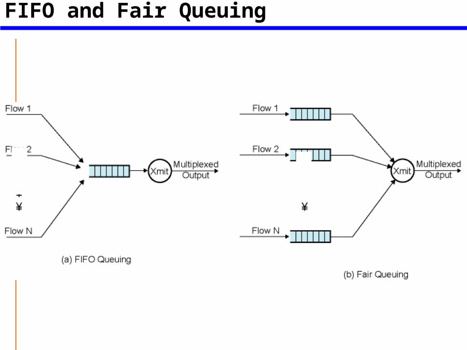
Figure 9.3 FIFO and Fair Queuing

Processor Sharing

Multiple queues as in FQSend one bit from each queue per round

Longer packets no longer get an advantageCan work out virtual (number of cycles) start and finish time for a given packetHowever, we wish to send packets, not bits

Bit-Round Fair Queuing (BRFQ)

Compute virtual start and finish time as beforeWhen a packet finished, the next packet sent is the one with the earliest virtual finish timeGood approximation to performance of PS

Throughput and delay converge as time increases

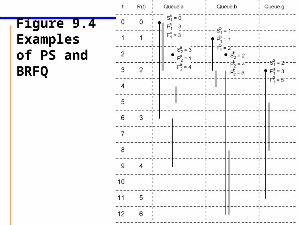
Figure 9.4 Examples of PS and BRFQ

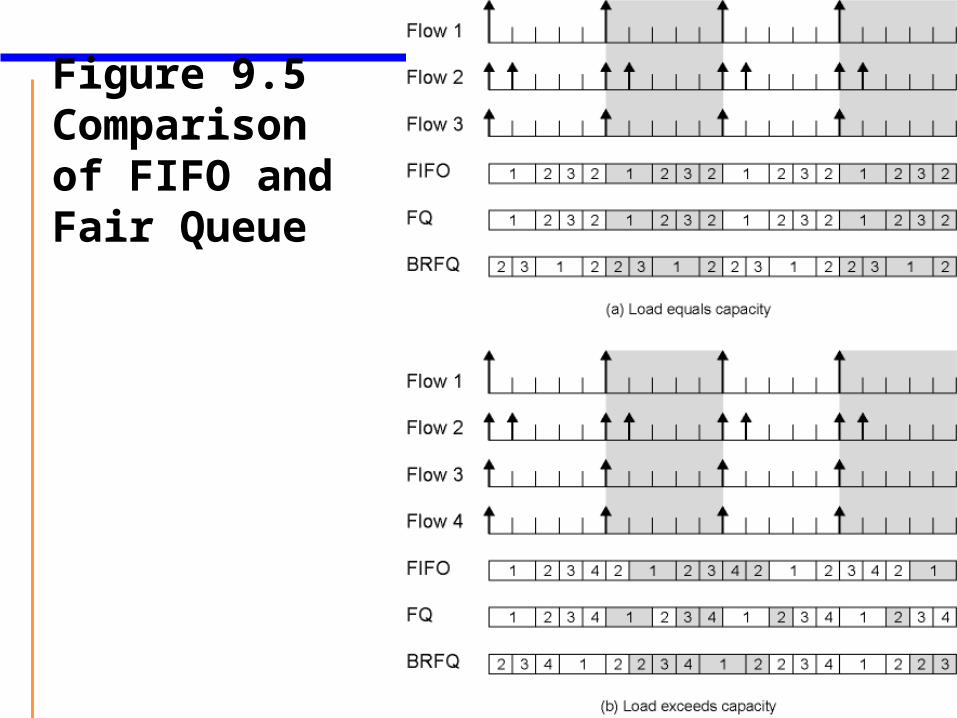
Figure 9.5Comparisonof FIFO andFair Queue

Generalized Processor Sharing (GPS)

BRFQ can not provide different capacities to different flowsEnhancement called Weighted fair queue (WFQ)From PS, allocate weighting to each flow that determines how many bots are sent during each round

If weighted 5, then 5 bits are sent per roundGives means of responding to different service requestsGuarantees that delays do not exceed bounds

Weighted Fair Queue

Emulates bit by bit GPSSame strategy as BRFQ

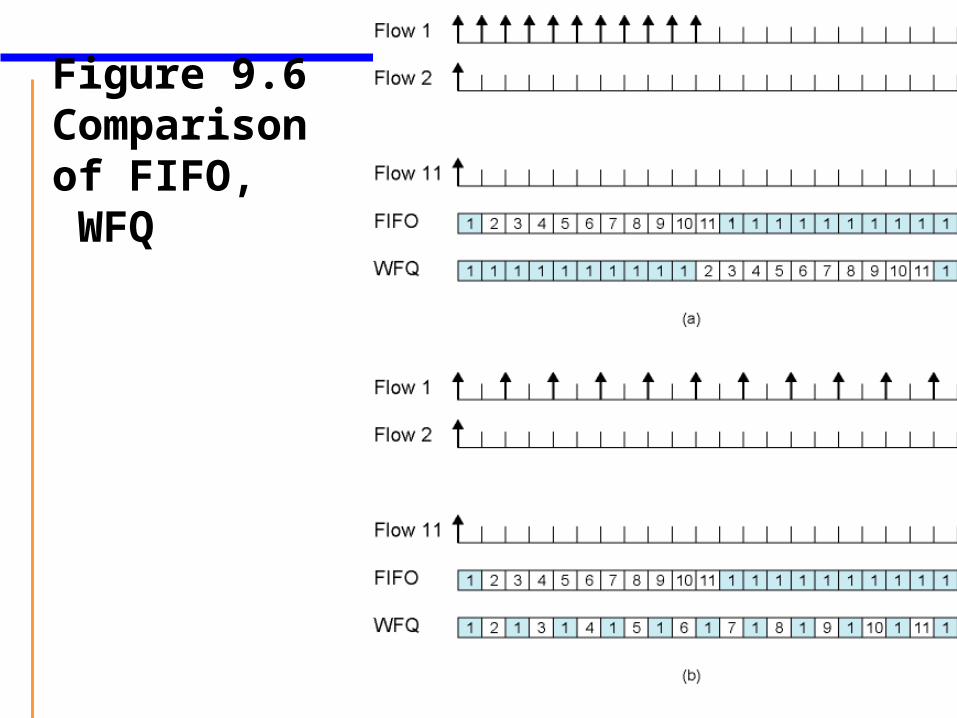
Figure 9.6Comparisonof FIFO, WFQ

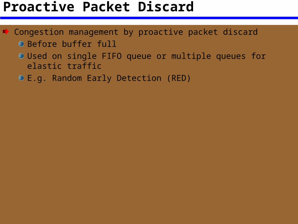
Proactive Packet Discard

Congestion management by proactive packet discardBefore buffer fullUsed on single FIFO queue or multiple queues for elastic trafficE.g. Random Early Detection (RED)

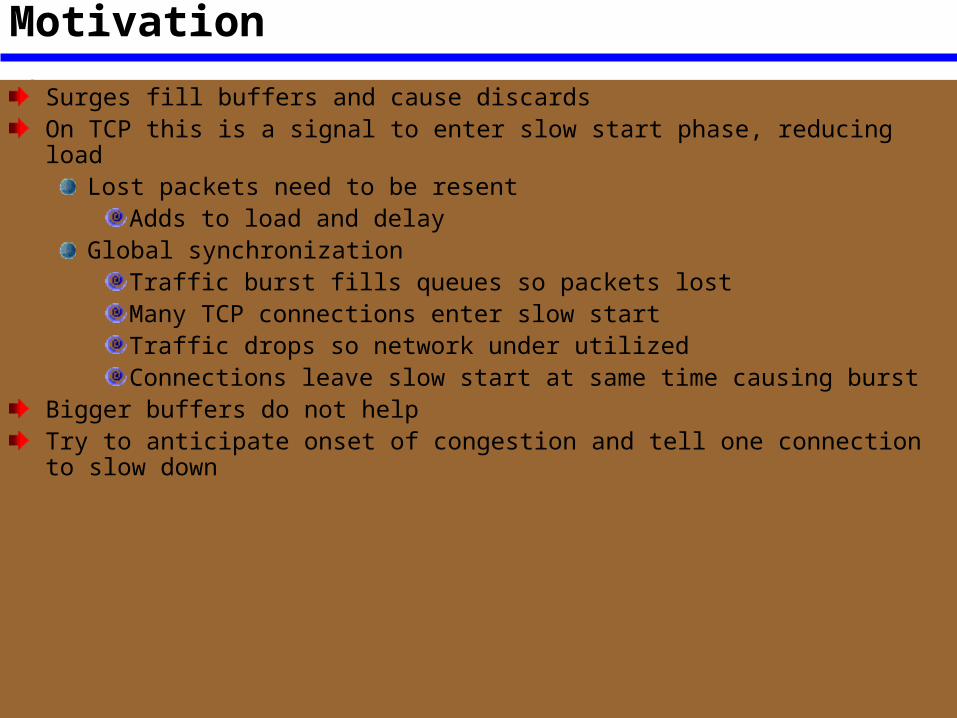
Random Early Detection (RED)Motivation

Surges fill buffers and cause discardsOn TCP this is a signal to enter slow start phase, reducing load

Lost packets need to be resentAdds to load and delay

Global synchronizationTraffic burst fills queues so packets lostMany TCP connections enter slow startTraffic drops so network under utilizedConnections leave slow start at same time causing burst

Bigger buffers do not helpTry to anticipate onset of congestion and tell one connection to slow down

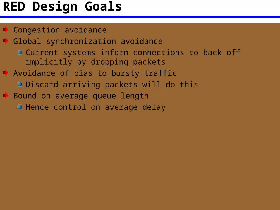
RED Design Goals

Congestion avoidanceGlobal synchronization avoidance

Current systems inform connections to back off implicitly by dropping packetsAvoidance of bias to bursty traffic

Discard arriving packets will do thisBound on average queue length

Hence control on average delay

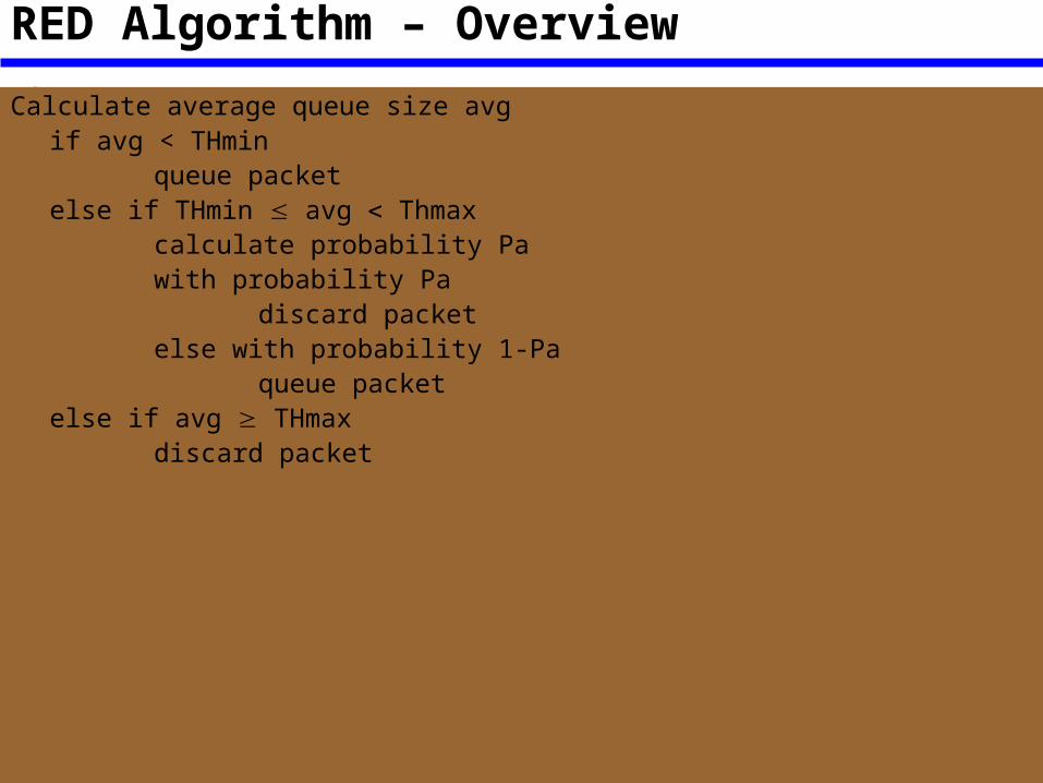
RED Algorithm – OverviewCalculate average queue size avg

if avg < THminqueue packet

else if THmin avg Thmaxcalculate probability Pawith probability Pa

discard packetelse with probability 1-Pa

queue packetelse if avg THmax

discard packet

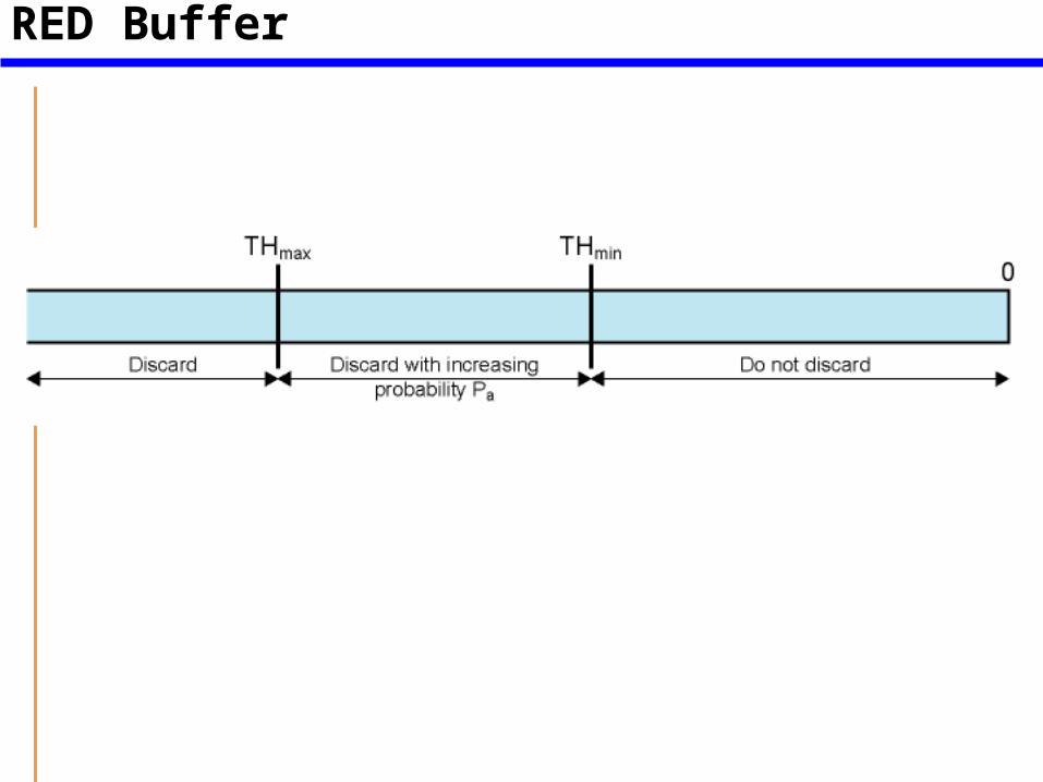
Figure 9.7RED Buffer

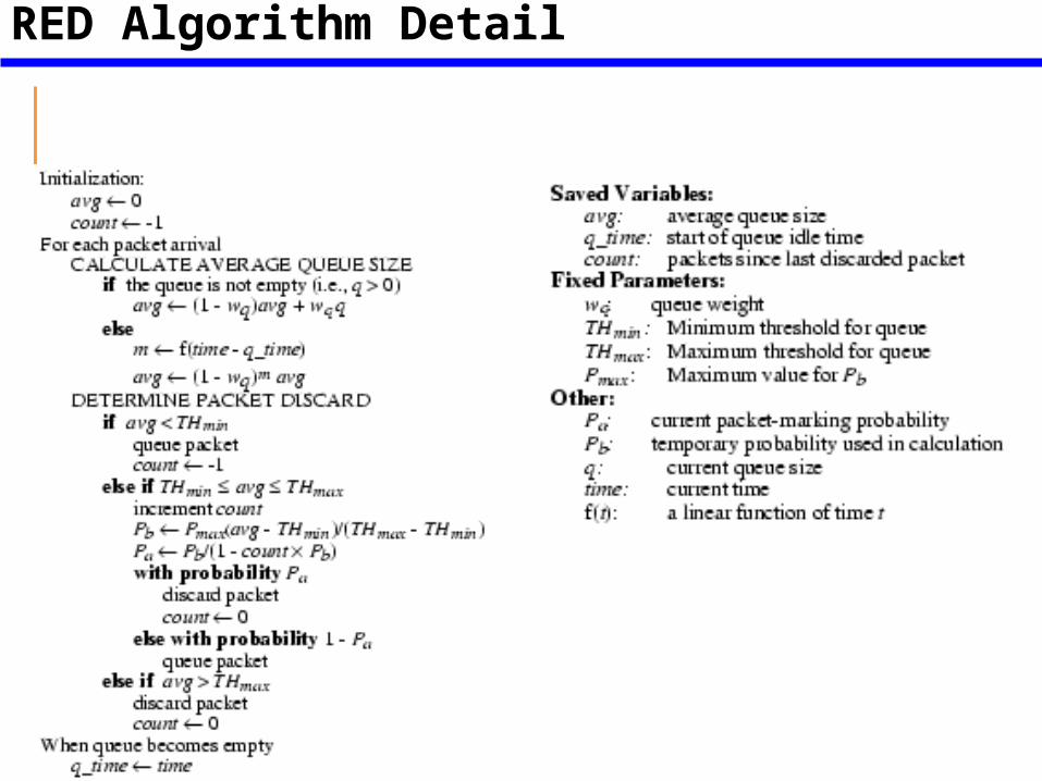
RED Algorithm Detail

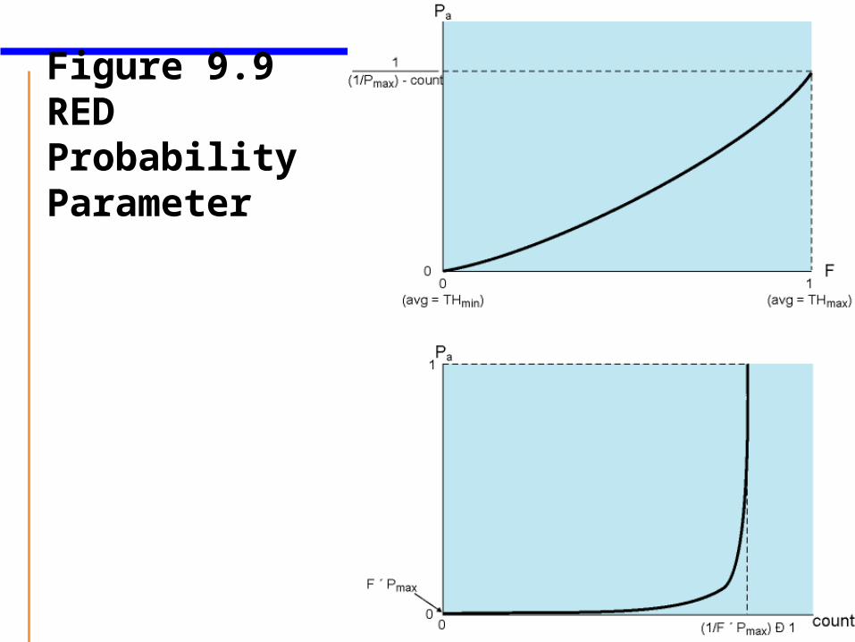
Figure 9.9RED ProbabilityParameter

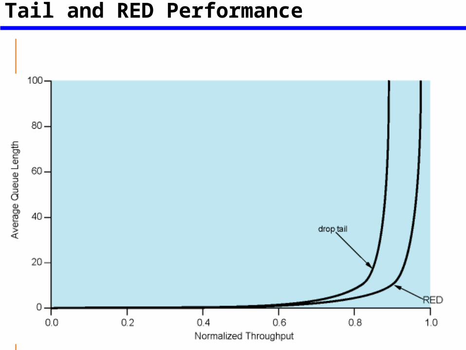
Figure 9.10 Comparison of Drop Tail and RED Performance

Differentiated Services (DS)

ISA and RSVP complex to deployMay not scale well for large volumes of traffic

Amount of control signalsMaintenance of state information at routers

DS architecture designed to provide simple, easy to implement, low overhead toolSupport range of network services

Differentiated on basis of performance

Characteristics of DSUse IPv4 header Type of Service or IPv6 Traffic Class field

No change to IPService level agreement (SLA) established between provider (internet domain) and customer prior to use of DS

DS mechanisms not needed in applicationsBuild in aggregation

All traffic with same DS field treated sameE.g. multiple voice connections

DS implemented in individual routers by queuing and forwarding based on DS fieldState information on flows not saved by routers

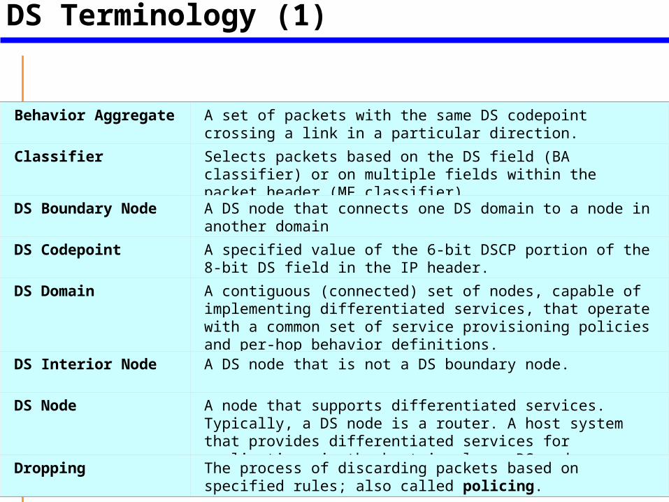
Table 9.1DS Terminology (1)

Behavior Aggregate

A set of packets with the same DS codepoint crossing a link in a particular direction.

Classifier Selects packets based on the DS field (BA classifier) or on multiple fields within the packet header (MF classifier).

DS Boundary Node A DS node that connects one DS domain to a node in another domain

DS Codepoint A specified value of the 6-bit DSCP portion of the 8-bit DS field in the IP header.

DS Domain A contiguous (connected) set of nodes, capable of implementing differentiated services, that operate with a common set of service provisioning policies and per-hop behavior definitions.

DS Interior Node A DS node that is not a DS boundary node.

DS Node A node that supports differentiated services. Typically, a DS node is a router. A host system that provides differentiated services for applications in the host is also a DS node.

Dropping The process of discarding packets based on specified rules; also called policing.

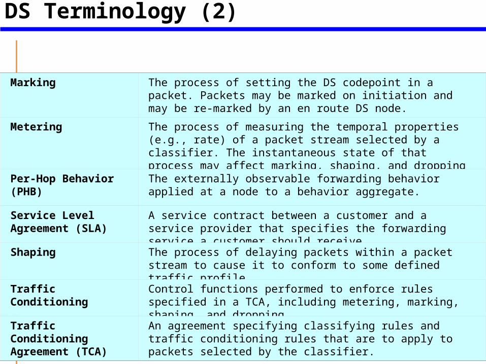
Table 9.1 DS Terminology (2)

Marking The process of setting the DS codepoint in a packet. Packets may be marked on initiation and may be re-marked by an en route DS node.

Metering The process of measuring the temporal properties (e.g., rate) of a packet stream selected by a classifier. The instantaneous state of that process may affect marking, shaping, and dropping functions.

Per-Hop Behavior (PHB)

The externally observable forwarding behavior applied at a node to a behavior aggregate.

Service Level Agreement (SLA)

A service contract between a customer and a service provider that specifies the forwarding service a customer should receive.

Shaping The process of delaying packets within a packet stream to cause it to conform to some defined traffic profile.

Traffic Conditioning

Control functions performed to enforce rules specified in a TCA, including metering, marking, shaping, and dropping.

Traffic Conditioning Agreement (TCA)

An agreement specifying classifying rules and traffic conditioning rules that are to apply to packets selected by the classifier.

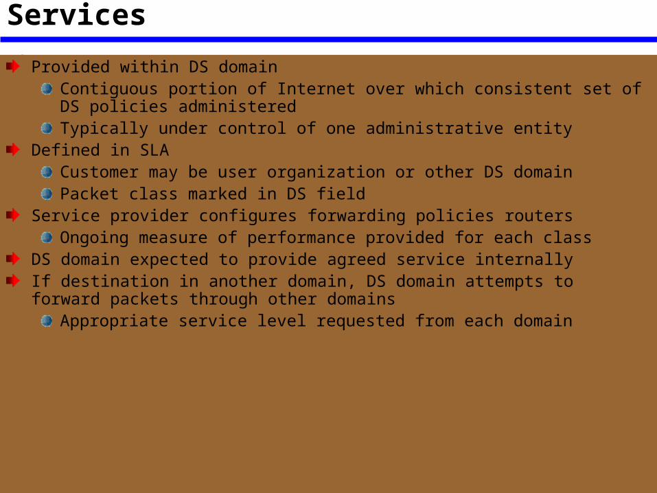
ServicesProvided within DS domain

Contiguous portion of Internet over which consistent set of DS policies administeredTypically under control of one administrative entity

Defined in SLACustomer may be user organization or other DS domainPacket class marked in DS field

Service provider configures forwarding policies routersOngoing measure of performance provided for each class

DS domain expected to provide agreed service internallyIf destination in another domain, DS domain attempts to forward packets through other domains

Appropriate service level requested from each domain

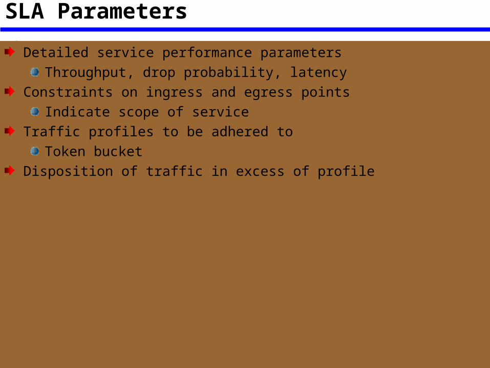
SLA Parameters

Detailed service performance parametersThroughput, drop probability, latency

Constraints on ingress and egress pointsIndicate scope of service

Traffic profiles to be adhered toToken bucket

Disposition of traffic in excess of profile

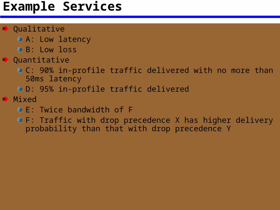
Example Services

QualitativeA: Low latencyB: Low loss

QuantitativeC: 90% in-profile traffic delivered with no more than 50ms latencyD: 95% in-profile traffic delivered

MixedE: Twice bandwidth of FF: Traffic with drop precedence X has higher delivery probability than that with drop precedence Y

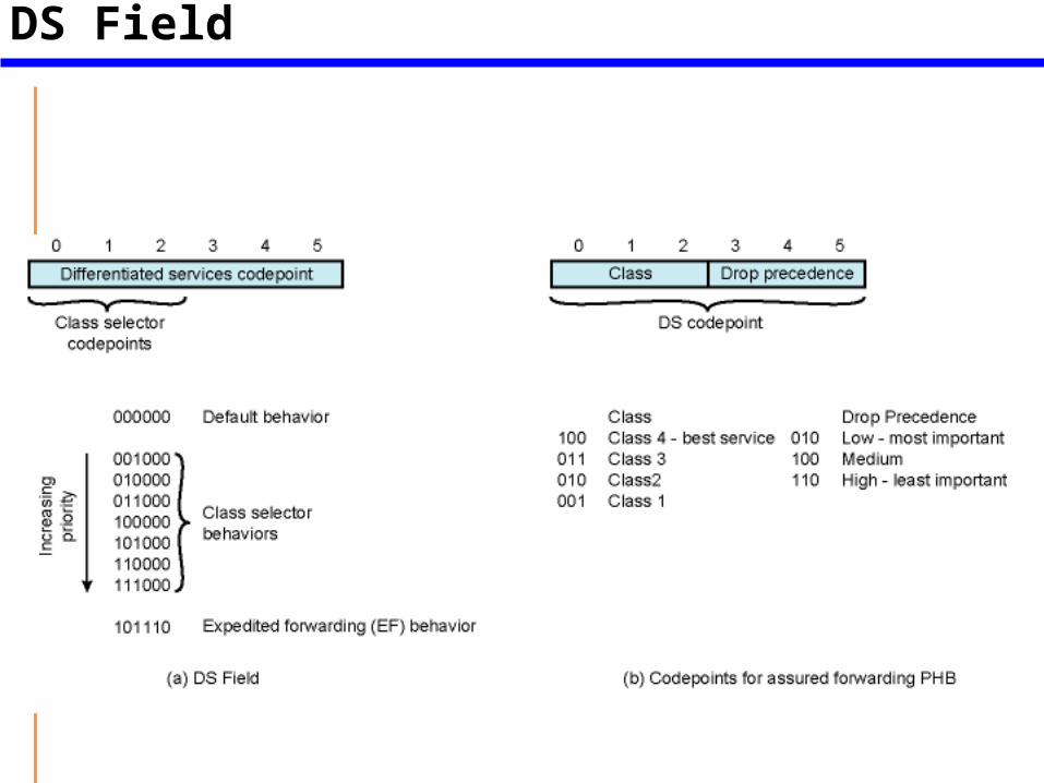
Figure 9.11DS Field

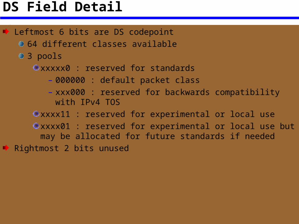
DS Field Detail

Leftmost 6 bits are DS codepoint64 different classes available3 pools

xxxxx0 : reserved for standards– 000000 : default packet class– xxx000 : reserved for backwards compatibility with IPv4 TOS

xxxx11 : reserved for experimental or local usexxxx01 : reserved for experimental or local use but may be allocated for future standards if needed

Rightmost 2 bits unused

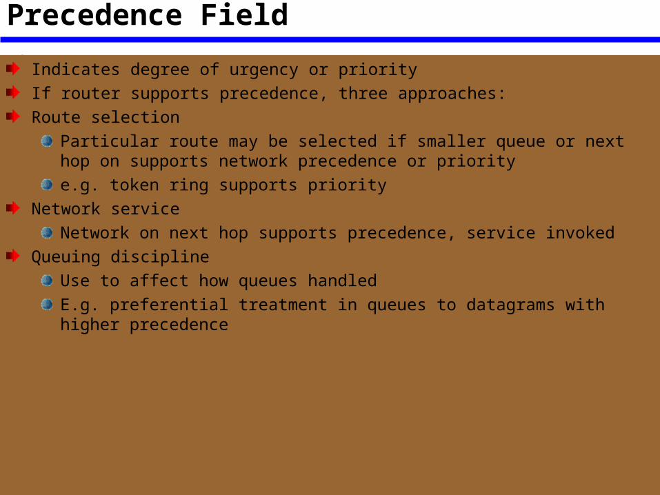
Precedence Field

Indicates degree of urgency or priority If router supports precedence, three approaches:Route selection

Particular route may be selected if smaller queue or next hop on supports network precedence or prioritye.g. token ring supports priority

Network serviceNetwork on next hop supports precedence, service invoked

Queuing disciplineUse to affect how queues handledE.g. preferential treatment in queues to datagrams with higher precedence

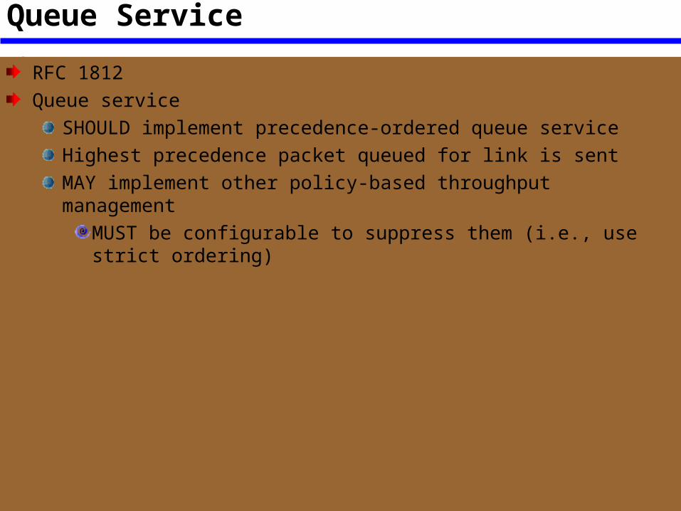
Router Queuing Disciplines – Queue Service

RFC 1812Queue service

SHOULD implement precedence-ordered queue serviceHighest precedence packet queued for link is sent MAY implement other policy-based throughput management

MUST be configurable to suppress them (i.e., use strict ordering)

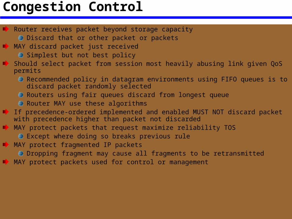
Router Queuing Disciplines – Congestion Control

Router receives packet beyond storage capacityDiscard that or other packet or packets

MAY discard packet just receivedSimplest but not best policy

Should select packet from session most heavily abusing link given QoS permitsRecommended policy in datagram environments using FIFO queues is to discard packet randomly selectedRouters using fair queues discard from longest queueRouter MAY use these algorithms

If precedence-ordered implemented and enabled MUST NOT discard packet with precedence higher than packet not discardedMAY protect packets that request maximize reliability TOS

Except where doing so breaks previous ruleMAY protect fragmented IP packets

Dropping fragment may cause all fragments to be retransmittedMAY protect packets used for control or management

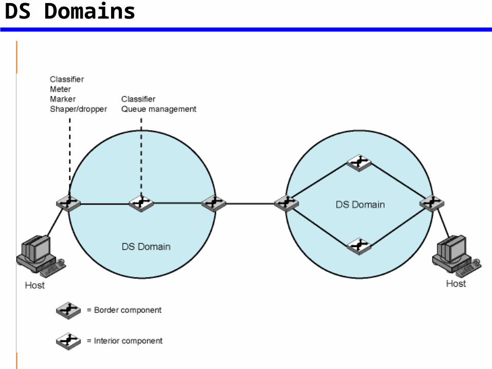
Figure 9.12DS Domains

Configuration – Interior Routers

Domain consists of set of contiguous routersInterpretation of DS codepoints within domain is consistentInterior nodes (routers) have simple mechanisms to handle packets based on codepoints

Queuing gives preferential treatment depending on codepointPer Hop behaviour (PHB)Must be available to all routersTypically the only part implemented in interior routers

Packet dropping rule dictated which to drop when buffer saturated

Configuration – Boundary Routers

Include PHB rulesAlso traffic conditioning to provide desired service

ClassifierSeparate packets into classes

MeterMeasure traffic for conformance to profile

MarkerPolicing by remarking codepoints if required

ShaperDropper

Per Hop Behaviour –Expedited forwarding

Premium serviceLow loss, delay, jitter; assured bandwidth end-to-end service through domainsLooks like point to point or leased lineDifficult to achieveConfigure nodes so traffic aggregate has well defined minimum departure rate

EF PHBCondition aggregate so arrival rate at any node is always less that minimum departure rate

Boundary conditioners

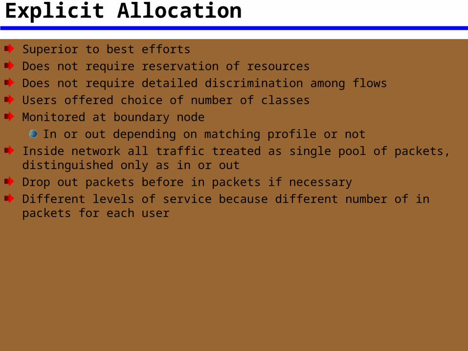
Per Hop Behaviour –Explicit Allocation

Superior to best effortsDoes not require reservation of resourcesDoes not require detailed discrimination among flowsUsers offered choice of number of classesMonitored at boundary node

In or out depending on matching profile or notInside network all traffic treated as single pool of packets, distinguished only as in or outDrop out packets before in packets if necessaryDifferent levels of service because different number of in packets for each user

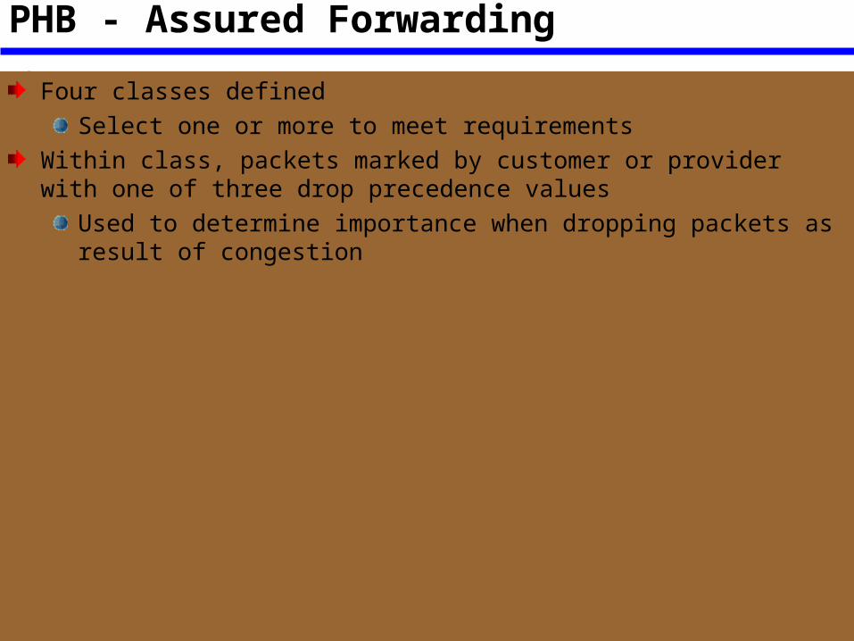
PHB - Assured Forwarding

Four classes definedSelect one or more to meet requirements

Within class, packets marked by customer or provider with one of three drop precedence values

Used to determine importance when dropping packets as result of congestion

UNIT VProtocols for QoS Support

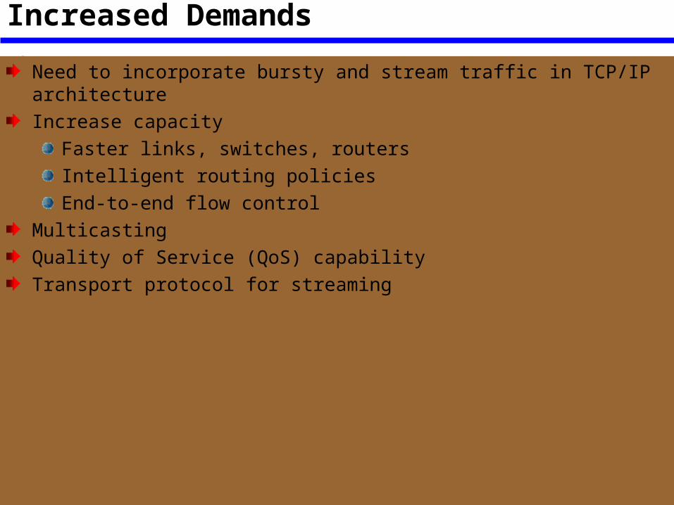
Increased Demands

Need to incorporate bursty and stream traffic in TCP/IP architectureIncrease capacity

Faster links, switches, routersIntelligent routing policiesEnd-to-end flow control

MulticastingQuality of Service (QoS) capabilityTransport protocol for streaming

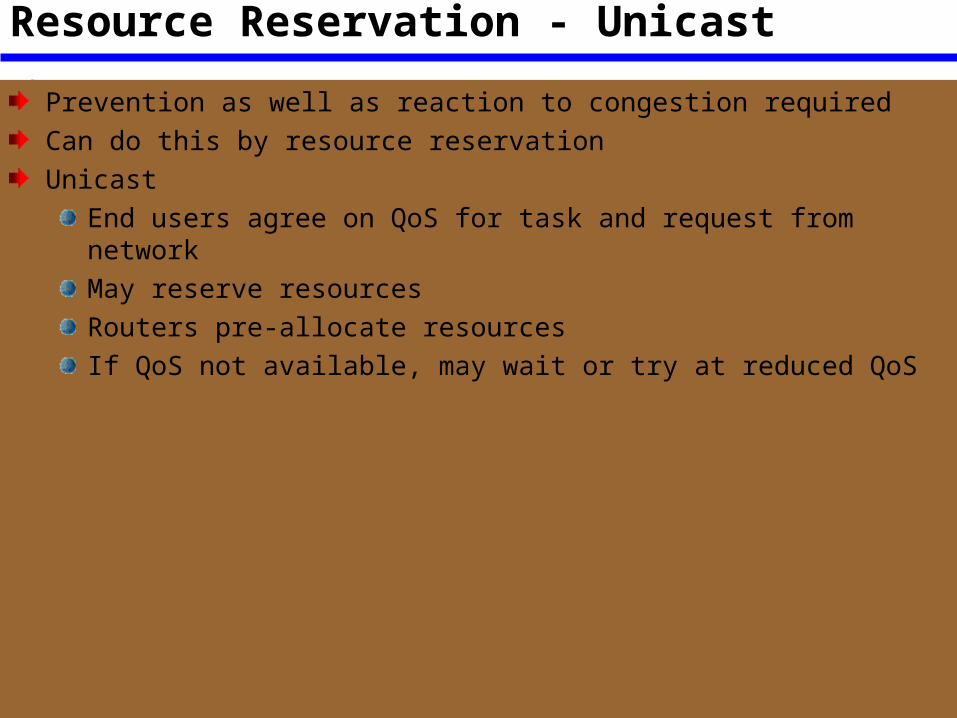
Resource Reservation - Unicast

Prevention as well as reaction to congestion requiredCan do this by resource reservationUnicast

End users agree on QoS for task and request from networkMay reserve resourcesRouters pre-allocate resourcesIf QoS not available, may wait or try at reduced QoS

Resource Reservation – Multicast

Generate vast trafficHigh volume application like videoLots of destinations

Can reduce loadSome members of group may not want current transmission

“Channels” of videoSome members may only be able to handle part of transmission

Basic and enhanced video components of video streamRouters can decide if they can meet demand

Resource Reservation Problems on an Internet

Must interact with dynamic routingReservations must follow changes in route

Soft state – a set of state information at a router that expires unless refreshedEnd users periodically renew resource requests

Resource ReSerVation Protocol (RSVP) Design Goals

Enable receivers to make reservationsDifferent reservations among members of same multicast group allowed

Deal gracefully with changes in group membershipDynamic reservations, separate for each member of group

Aggregate for group should reflect resources neededTake into account common path to different members of group

Receivers can select one of multiple sources (channel selection)Deal gracefully with changes in routes

Re-establish reservationsControl protocol overheadIndependent of routing protocol

RSVP CharacteristicsUnicast and MulticastSimplex

Unidirectional data flowSeparate reservations in two directions

Receiver initiatedReceiver knows which subset of source transmissions it wants

Maintain soft state in internetResponsibility of end users

Providing different reservation stylesUsers specify how reservations for groups are aggregated

Transparent operation through non-RSVP routersSupport IPv4 (ToS field) and IPv6 (Flow label field)

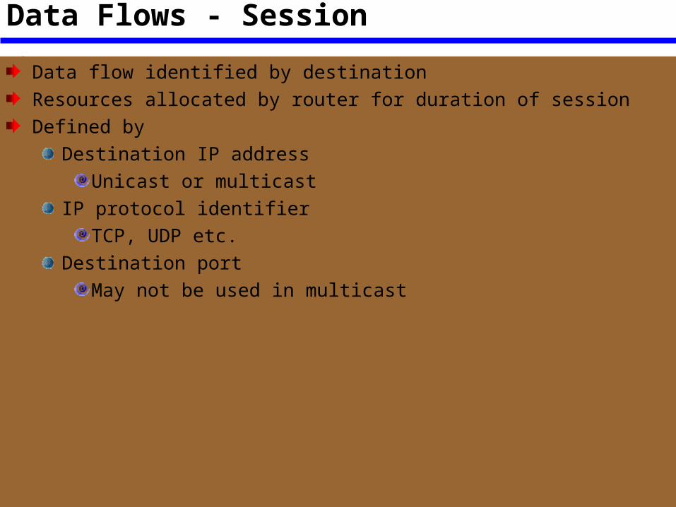
Data Flows - Session

Data flow identified by destinationResources allocated by router for duration of sessionDefined by

Destination IP addressUnicast or multicast

IP protocol identifierTCP, UDP etc.

Destination portMay not be used in multicast

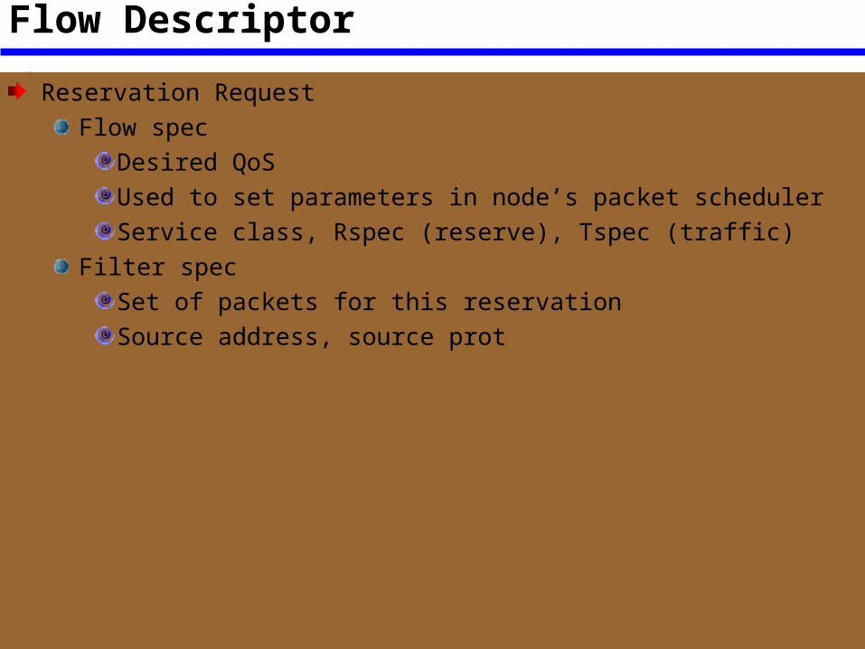
Flow Descriptor

Reservation RequestFlow spec

Desired QoSUsed to set parameters in node’s packet schedulerService class, Rspec (reserve), Tspec (traffic)

Filter specSet of packets for this reservationSource address, source prot

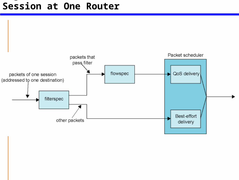
Figure 10.1 Treatment of Packets of One Session at One Router

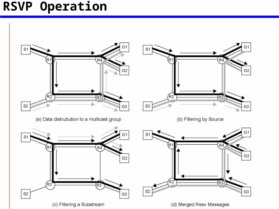
Figure 10.2 RSVP Operation

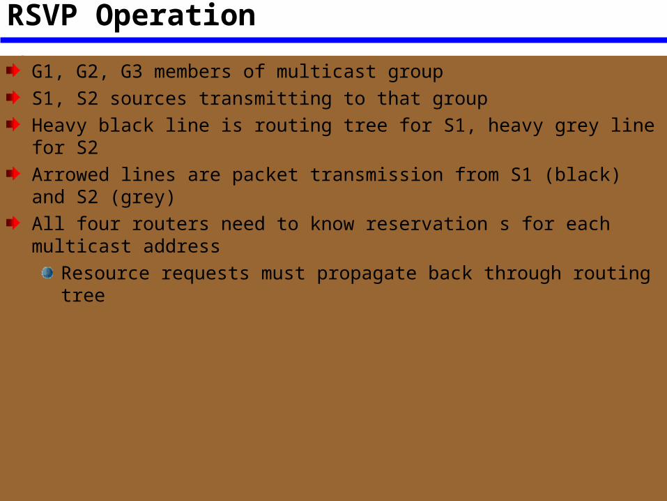
RSVP Operation

G1, G2, G3 members of multicast groupS1, S2 sources transmitting to that groupHeavy black line is routing tree for S1, heavy grey line for S2Arrowed lines are packet transmission from S1 (black) and S2 (grey)All four routers need to know reservation s for each multicast address

Resource requests must propagate back through routing tree

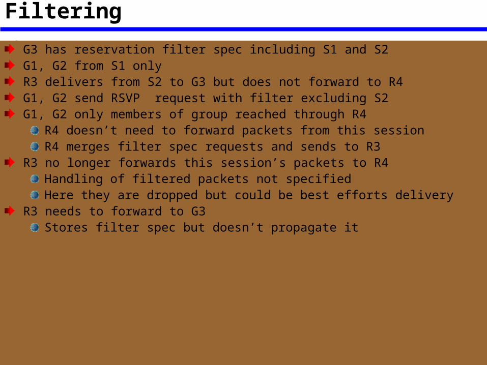
FilteringG3 has reservation filter spec including S1 and S2G1, G2 from S1 onlyR3 delivers from S2 to G3 but does not forward to R4G1, G2 send RSVP request with filter excluding S2G1, G2 only members of group reached through R4

R4 doesn’t need to forward packets from this sessionR4 merges filter spec requests and sends to R3

R3 no longer forwards this session’s packets to R4Handling of filtered packets not specifiedHere they are dropped but could be best efforts delivery

R3 needs to forward to G3Stores filter spec but doesn’t propagate it

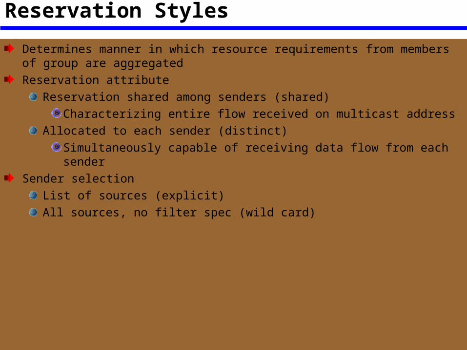
Reservation Styles

Determines manner in which resource requirements from members of group are aggregatedReservation attribute

Reservation shared among senders (shared)Characterizing entire flow received on multicast address

Allocated to each sender (distinct)Simultaneously capable of receiving data flow from each sender

Sender selectionList of sources (explicit)All sources, no filter spec (wild card)

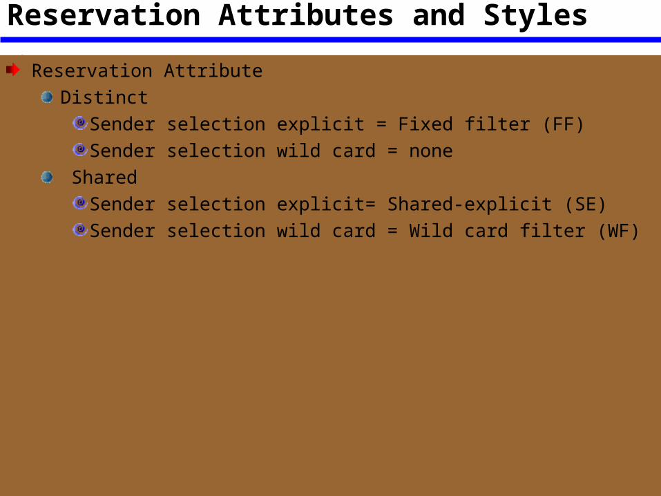
Reservation Attributes and Styles

Reservation AttributeDistinct

Sender selection explicit = Fixed filter (FF)Sender selection wild card = none

SharedSender selection explicit= Shared-explicit (SE)Sender selection wild card = Wild card filter (WF)

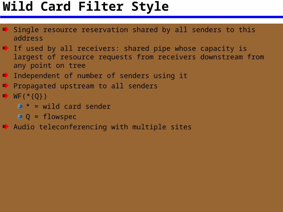
Wild Card Filter Style

Single resource reservation shared by all senders to this addressIf used by all receivers: shared pipe whose capacity is largest of resource requests from receivers downstream from any point on treeIndependent of number of senders using itPropagated upstream to all sendersWF(*{Q})

* = wild card senderQ = flowspec

Audio teleconferencing with multiple sites

Fixed Filter Style

Distinct reservation for each senderExplicit list of sendersFF(S1{Q!}, S2{Q2},…)Video distribution

Shared Explicit Style

Single reservation shared among specific list of sendersSE(S1, S2, S3, …{Q})Multicast applications with multiple data sources but unlikely to transmit simultaneously

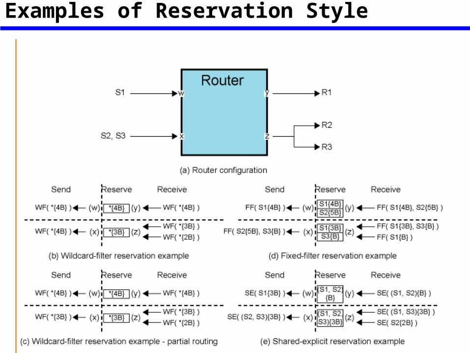
Figure 10.3Examples of Reservation Style

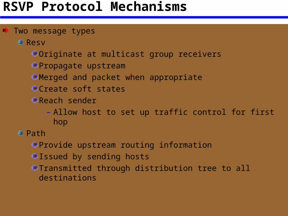
RSVP Protocol Mechanisms

Two message typesResv

Originate at multicast group receiversPropagate upstreamMerged and packet when appropriateCreate soft statesReach sender

– Allow host to set up traffic control for first hopPath

Provide upstream routing informationIssued by sending hostsTransmitted through distribution tree to all destinations

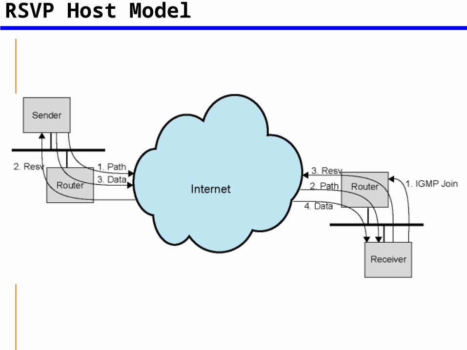
Figure 10.4RSVP Host Model

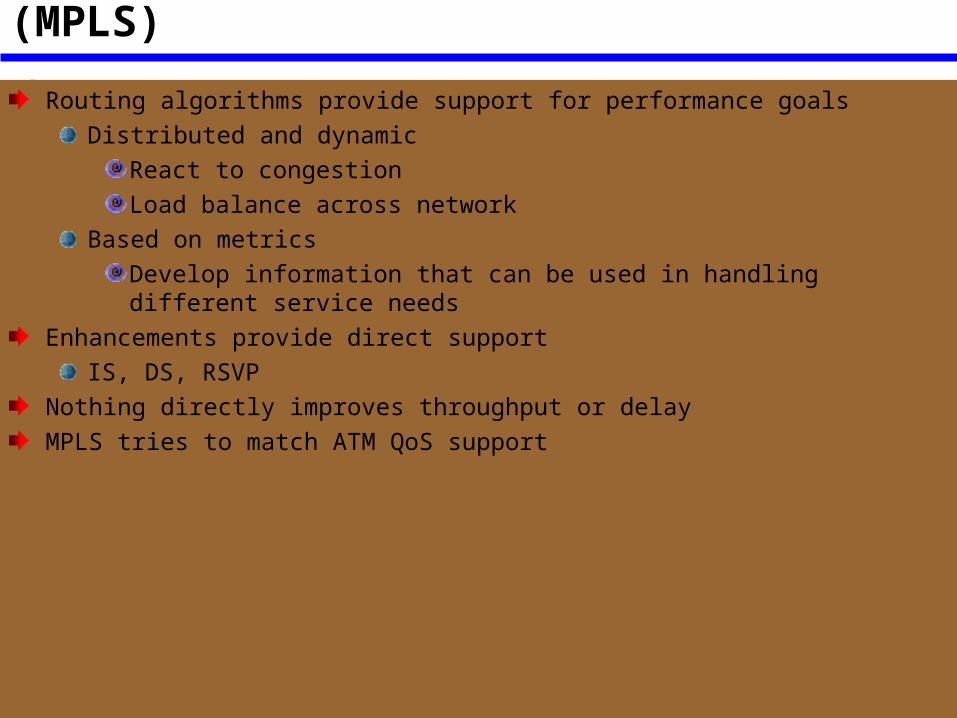
Multiprotocol Label Switching (MPLS)

Routing algorithms provide support for performance goalsDistributed and dynamic

React to congestionLoad balance across network

Based on metricsDevelop information that can be used in handling different service needs

Enhancements provide direct supportIS, DS, RSVP

Nothing directly improves throughput or delayMPLS tries to match ATM QoS support

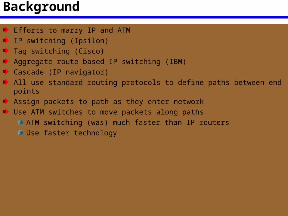
Background

Efforts to marry IP and ATMIP switching (Ipsilon)Tag switching (Cisco)Aggregate route based IP switching (IBM)Cascade (IP navigator)All use standard routing protocols to define paths between end pointsAssign packets to path as they enter networkUse ATM switches to move packets along paths

ATM switching (was) much faster than IP routersUse faster technology

Developments

IETF working group 1997Proposed standard 2001Routers developed to be as fast as ATM switches

Remove the need to provide both technologies in same networkMPLS does provide new capabilities

QoS supportTraffic engineeringVirtual private networksMultiprotocol support

Connection Oriented QoS Support

Guarantee fixed capacity for specific applicationsControl latency/jitterEnsure capacity for voiceProvide specific, guaranteed quantifiable SLAsConfigure varying degrees of QoS for multiple customersMPLS imposes connection oriented framework on IP based internets

Traffic Engineering

Ability to dynamically define routes, plan resource commitments based on known demands and optimize network utilizationBasic IP allows primitive traffic engineering

E.g. dynamic routingMPLS makes network resource commitment easy

Able to balance load in face of demandAble to commit to different levels of support to meet user traffic requirementsAware of traffic flows with QoS requirements and predicted demandIntelligent re-routing when congested

VPN Support

Traffic from a given enterprise or group passes transparently through an internetSegregated from other traffic on internetPerformance guaranteesSecurity

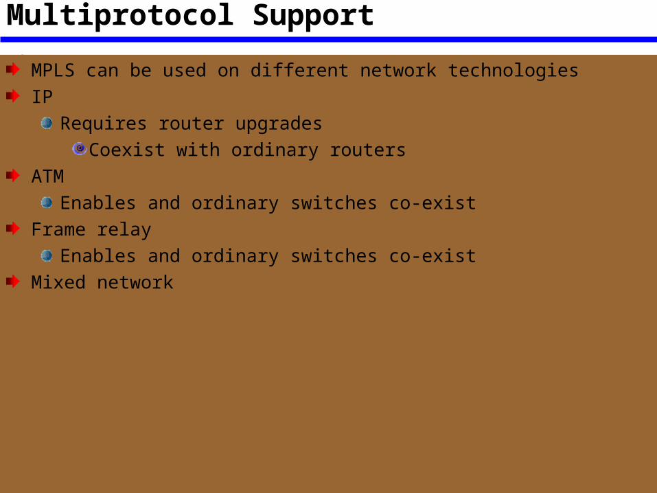
Multiprotocol Support

MPLS can be used on different network technologiesIP

Requires router upgradesCoexist with ordinary routers

ATMEnables and ordinary switches co-exist

Frame relayEnables and ordinary switches co-exist

Mixed network

MPLS Terminology

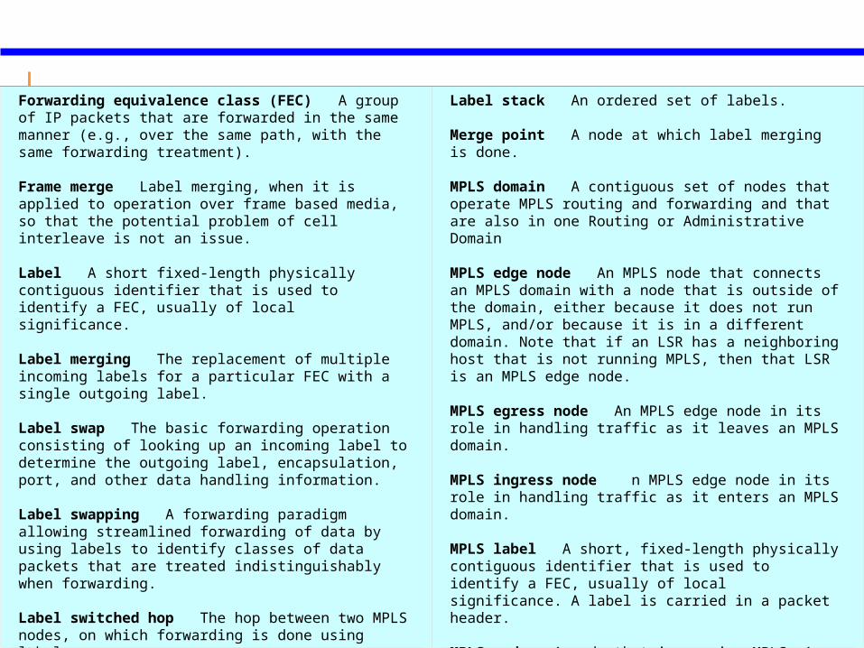
Forwarding equivalence class (FEC) A group of IP packets that are forwarded in the same manner (e.g., over the same path, with the same forwarding treatment). Frame merge Label merging, when it is applied to operation over frame based media, so that the potential problem of cell interleave is not an issue. Label A short fixed-length physically contiguous identifier that is used to identify a FEC, usually of local significance. Label merging The replacement of multiple incoming labels for a particular FEC with a single outgoing label. Label swap The basic forwarding operation consisting of looking up an incoming label to determine the outgoing label, encapsulation, port, and other data handling information. Label swapping A forwarding paradigm allowing streamlined forwarding of data by using labels to identify classes of data packets that are treated indistinguishably when forwarding. Label switched hop The hop between two MPLS nodes, on which forwarding is done using labels. Label switched path The path through one or more LSRs at one level of the hierarchy followed by a packets in a particular FEC. Label switching router (LSR) An MPLS node that is capable of forwarding native L3 packets. 

Label stack An ordered set of labels. Merge point A node at which label merging is done. MPLS domain A contiguous set of nodes that operate MPLS routing and forwarding and that are also in one Routing or Administrative Domain MPLS edge node An MPLS node that connects an MPLS domain with a node that is outside of the domain, either because it does not run MPLS, and/or because it is in a different domain. Note that if an LSR has a neighboring host that is not running MPLS, then that LSR is an MPLS edge node. MPLS egress node An MPLS edge node in its role in handling traffic as it leaves an MPLS domain. MPLS ingress node n MPLS edge node in its role in handling traffic as it enters an MPLS domain. MPLS label A short, fixed-length physically contiguous identifier that is used to identify a FEC, usually of local significance. A label is carried in a packet header. MPLS node A node that is running MPLS. An MPLS node will be aware of MPLS control protocols, will operate one or more L3 routing protocols, and will be capable of forwarding packets based on labels. An MPLS node may optionally be also capable of forwarding native L3 packets.

MPLS Operation

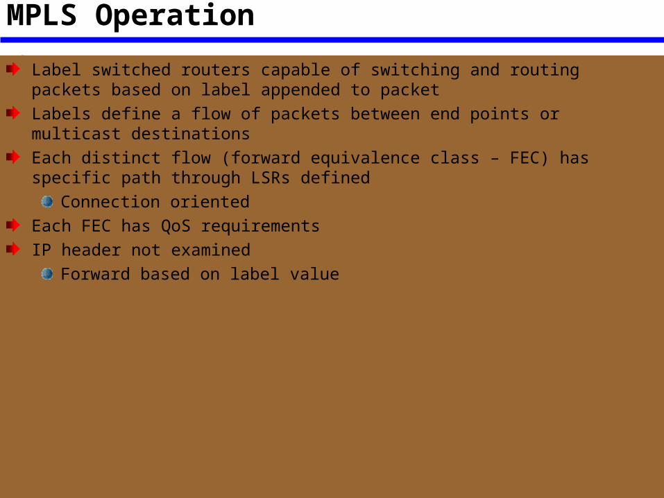
Label switched routers capable of switching and routing packets based on label appended to packetLabels define a flow of packets between end points or multicast destinationsEach distinct flow (forward equivalence class – FEC) has specific path through LSRs defined

Connection orientedEach FEC has QoS requirementsIP header not examined

Forward based on label value

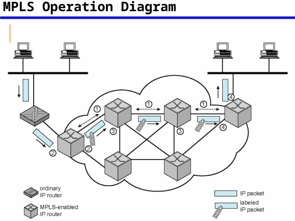
Figure 10.5MPLS Operation Diagram

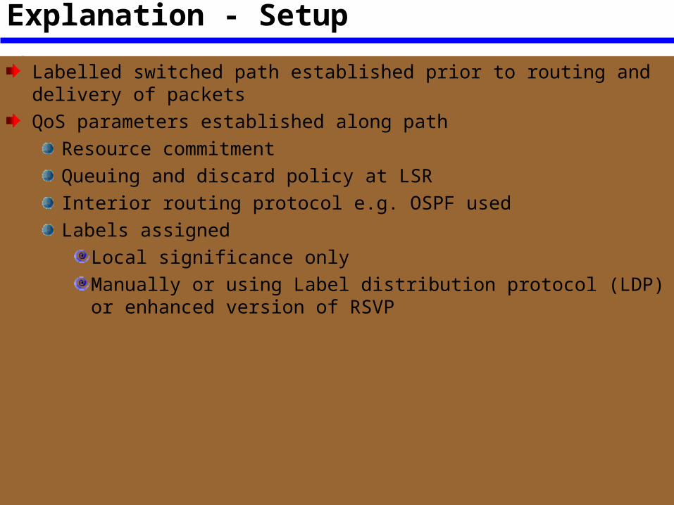
Explanation - Setup

Labelled switched path established prior to routing and delivery of packetsQoS parameters established along path

Resource commitmentQueuing and discard policy at LSRInterior routing protocol e.g. OSPF usedLabels assigned

Local significance onlyManually or using Label distribution protocol (LDP) or enhanced version of RSVP

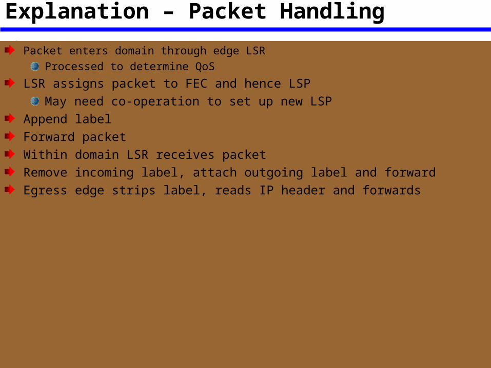
Explanation – Packet Handling

Packet enters domain through edge LSRProcessed to determine QoS

LSR assigns packet to FEC and hence LSPMay need co-operation to set up new LSP

Append labelForward packetWithin domain LSR receives packetRemove incoming label, attach outgoing label and forwardEgress edge strips label, reads IP header and forwards

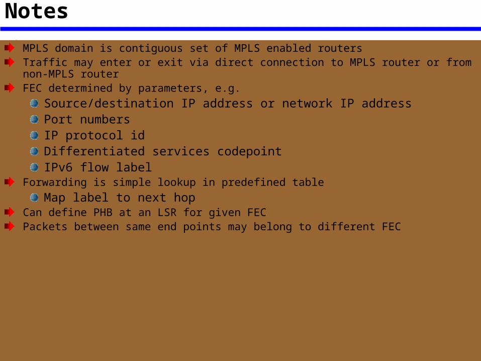
NotesMPLS domain is contiguous set of MPLS enabled routersTraffic may enter or exit via direct connection to MPLS router or from non-MPLS routerFEC determined by parameters, e.g.

Source/destination IP address or network IP addressPort numbersIP protocol idDifferentiated services codepointIPv6 flow label

Forwarding is simple lookup in predefined tableMap label to next hop

Can define PHB at an LSR for given FECPackets between same end points may belong to different FEC

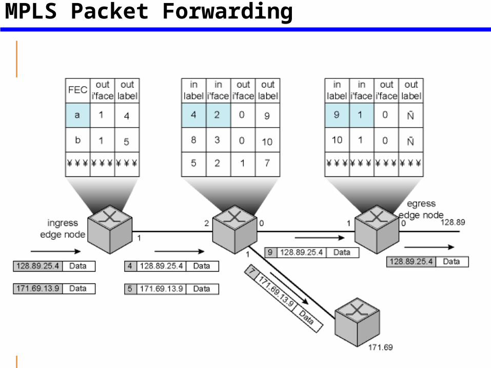
Figure 10.6MPLS Packet Forwarding

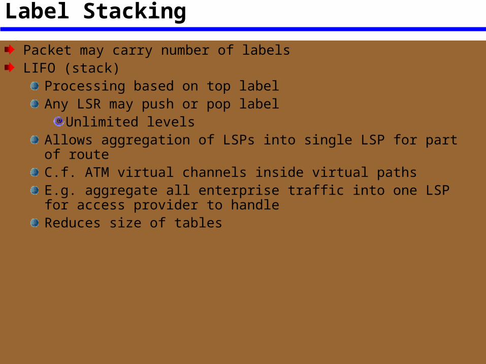
Label Stacking

Packet may carry number of labelsLIFO (stack)

Processing based on top labelAny LSR may push or pop label

Unlimited levelsAllows aggregation of LSPs into single LSP for part of routeC.f. ATM virtual channels inside virtual pathsE.g. aggregate all enterprise traffic into one LSP for access provider to handleReduces size of tables

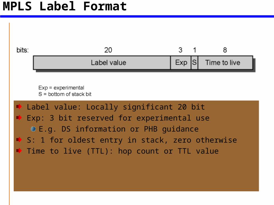
Figure 10.7 MPLS Label Format

Label value: Locally significant 20 bitExp: 3 bit reserved for experimental use

E.g. DS information or PHB guidanceS: 1 for oldest entry in stack, zero otherwiseTime to live (TTL): hop count or TTL value

Time to Live Processing

Needed to support TTL since IP header not readFirst label TTL set to IP header TTL on entry to MPLS domainTTL of top entry on stack decremented at internal LSR

If zero, packet dropped or passed to ordinary error processing (e.g. ICMP)If positive, value placed in TTL of top label on stack and packet forwarded

At exit from domain, (single stack entry) TTL decrementedIf zero, as aboveIf positive, placed in TTL field of Ip header and forwarded

Label Stack

Appear after data link layer header, before network layer headerTop of stack is earliest (closest to network layer header)Network layer packet follows label stack entry with S=1Over connection oriented services

Topmost label value in ATM header VPI/VCI fieldFacilitates ATM switching

Top label inserted between cell header and IP headerIn DLCI field of Frame RelayNote: TTL problem

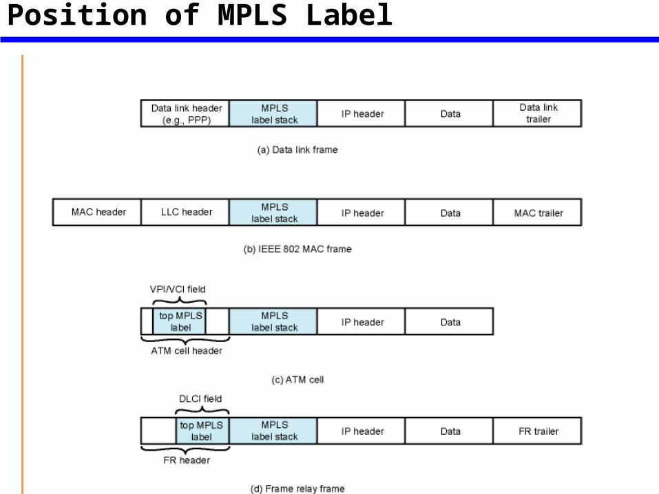
Figure 10.8Position of MPLS Label

FECs, LSPs, and LabelsTraffic grouped into FECsTraffic in a FEC transits an MLPS domain along an LSPPackets identified by locally significant labelAt each LSR, labelled packets forwarded on basis of label.

LSR replaces incoming label with outgoing labelEach flow must be assigned to a FECRouting protocol must determine topology and current conditions so LSP can be assigned to FEC

Must be able to gather and use information to support QoS LSRs must be aware of LSP for given FEC, assign incoming label to LSP, communicate label to other LSRs

Topology of LSPs

Unique ingress and egress LSRSingle path through domain

Unique egress, multiple ingress LSRsMultiple paths, possibly sharing final few hops

Multiple egress LSRs for unicast trafficMulticast

Route Selection

Selection of LSP for particular FECHop-by-hop

LSR independently chooses next hopOrdinary routing protocols e.g. OSPFDoesn’t support traffic engineering or policy routing

ExplicitLSR (usually ingress or egress) specifies some or all LSRs in LSP for given FECSelected by configuration,or dynamically

Constraint Based Routing Algorithm

Take in to account traffic requirements of flows and resources available along hopsCurrent utilization, existing capacity, committed servicesAdditional metrics over and above traditional routing protocols (OSPF)

Max link data rateCurrent capacity reservationPacket loss ratioLink propagation delay

Label Distribution

Setting up LSPAssign label to LSPInform all potential upstream nodes of label assigned by LSR to FEC

Allows proper packet labellingLearn next hop for LSP and label that downstream node has assigned to FEC

Allow LSR to map incoming to outgoing label

Real Time Transport Protocol

TCP not suited to real time distributed applicationPoint to point so not suitable for multicastRetransmitted segments arrive out of orderNo way to associate timing with segments

UDP does not include timing information nor any support for real time applicationsSolution is real-time transport protocol RTP

RTP Architecture

Close coupling between protocol and application layer functionalityFramework for application to implement single protocol

Application level framingIntegrated layer processing

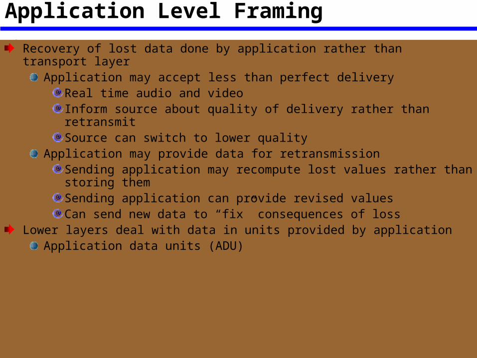
Application Level FramingRecovery of lost data done by application rather than transport layer

Application may accept less than perfect deliveryReal time audio and videoInform source about quality of delivery rather than retransmitSource can switch to lower quality

Application may provide data for retransmissionSending application may recompute lost values rather than storing themSending application can provide revised valuesCan send new data to “fix” consequences of loss

Lower layers deal with data in units provided by applicationApplication data units (ADU)

Integrated Layer Processing

Adjacent layers in protocol stack tightly coupledAllows out of order or parallel functions from different layers

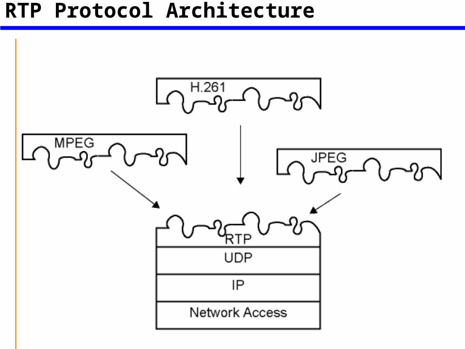
Figure 10.9RTP Protocol Architecture

RTP Data Transfer Protocol

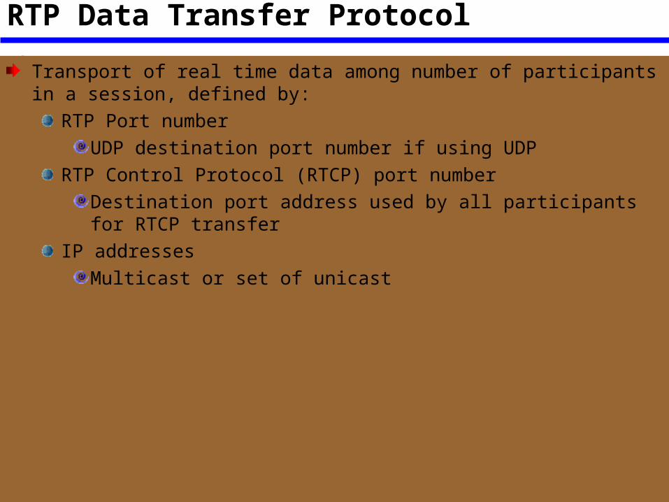
Transport of real time data among number of participants in a session, defined by:RTP Port number

UDP destination port number if using UDPRTP Control Protocol (RTCP) port number

Destination port address used by all participants for RTCP transferIP addresses

Multicast or set of unicast

Multicast Support

Each RTP data unit includes:Source identifierTimestampPayload format

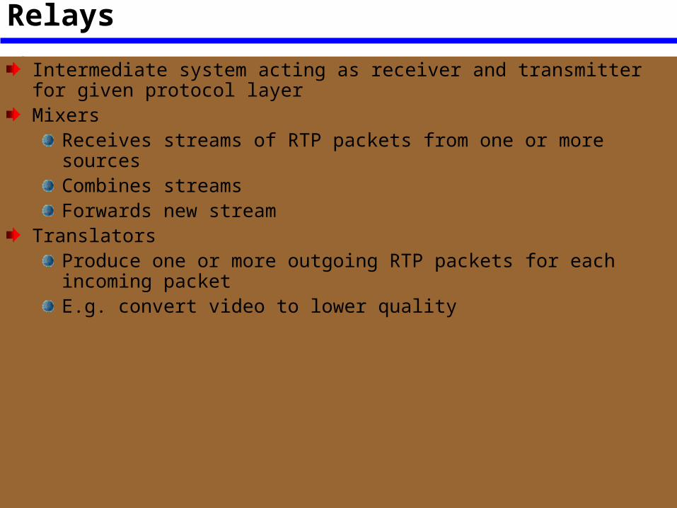
Relays

Intermediate system acting as receiver and transmitter for given protocol layerMixers

Receives streams of RTP packets from one or more sourcesCombines streamsForwards new stream

TranslatorsProduce one or more outgoing RTP packets for each incoming packetE.g. convert video to lower quality

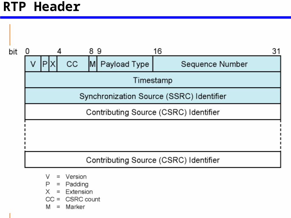
Figure 10.10RTP Header

RTP Control Protocol (RTCP)

RTP is for user dataRTCP is multicast provision of feedback to sources and session participantsUses same underlying transport protocol (usually UDP) and different port numberRTCP packet issued periodically by each participant to other session members

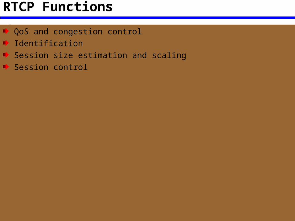
RTCP Functions

QoS and congestion controlIdentificationSession size estimation and scalingSession control

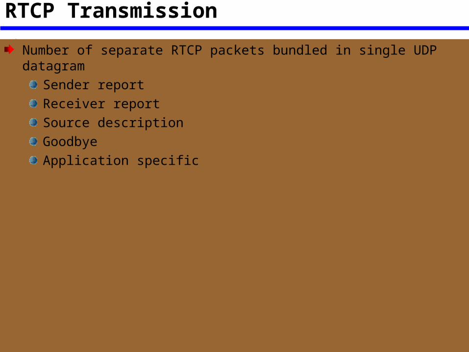
RTCP Transmission

Number of separate RTCP packets bundled in single UDP datagramSender reportReceiver reportSource descriptionGoodbyeApplication specific

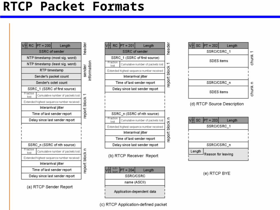
Figure 10.11RTCP Packet Formats

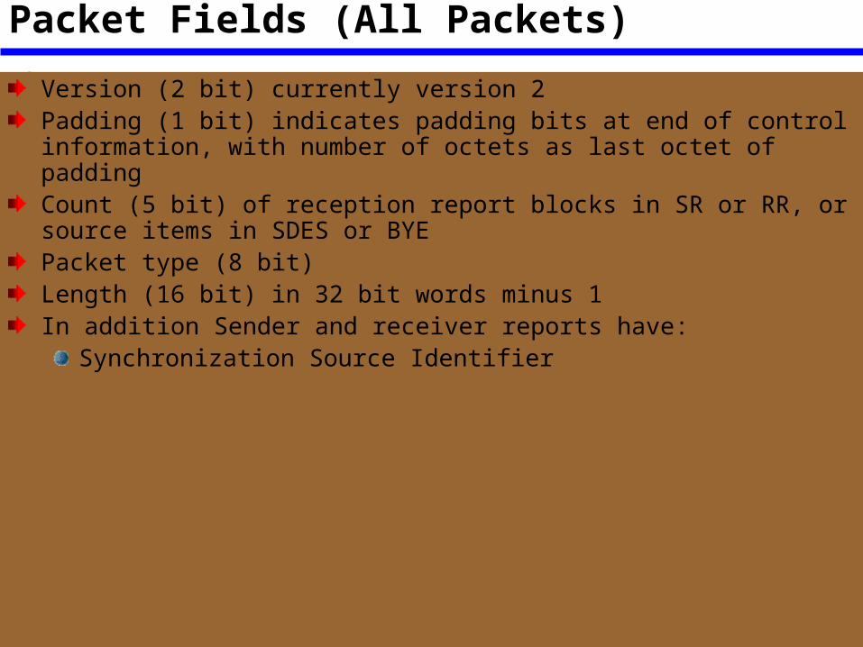
Packet Fields (All Packets)

Version (2 bit) currently version 2Padding (1 bit) indicates padding bits at end of control information, with number of octets as last octet of paddingCount (5 bit) of reception report blocks in SR or RR, or source items in SDES or BYEPacket type (8 bit)Length (16 bit) in 32 bit words minus 1In addition Sender and receiver reports have:

Synchronization Source Identifier

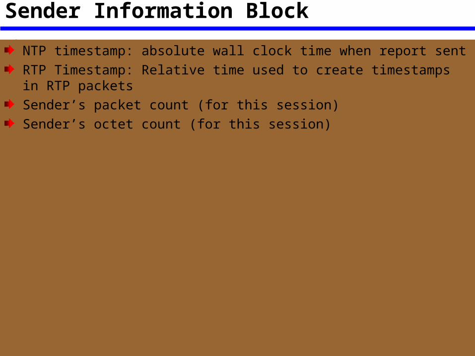
Packet Fields (Sender Report)Sender Information Block

NTP timestamp: absolute wall clock time when report sentRTP Timestamp: Relative time used to create timestamps in RTP packetsSender’s packet count (for this session)Sender’s octet count (for this session)

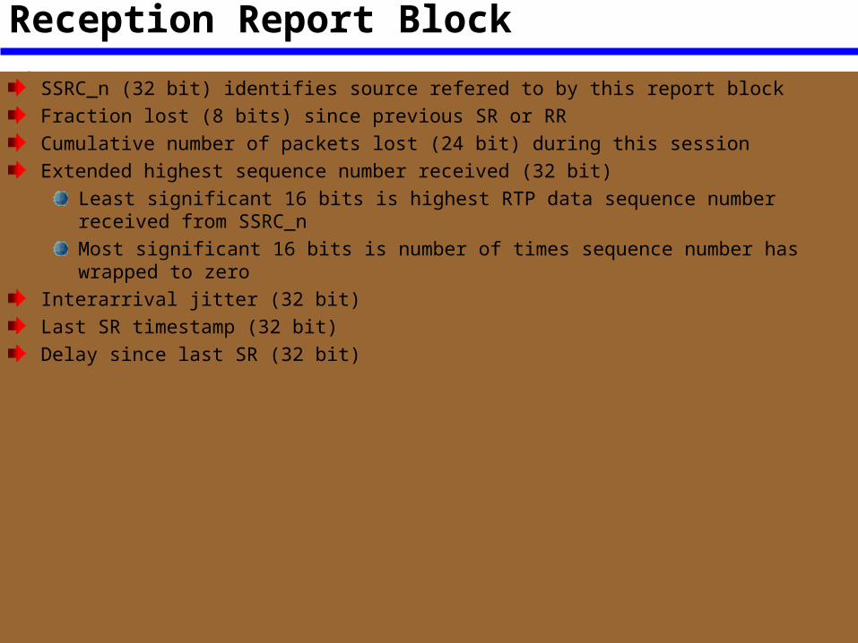
Packet Fields (Sender Report)Reception Report Block

SSRC_n (32 bit) identifies source refered to by this report blockFraction lost (8 bits) since previous SR or RRCumulative number of packets lost (24 bit) during this sessionExtended highest sequence number received (32 bit)

Least significant 16 bits is highest RTP data sequence number received from SSRC_nMost significant 16 bits is number of times sequence number has wrapped to zero

Interarrival jitter (32 bit)Last SR timestamp (32 bit)Delay since last SR (32 bit)

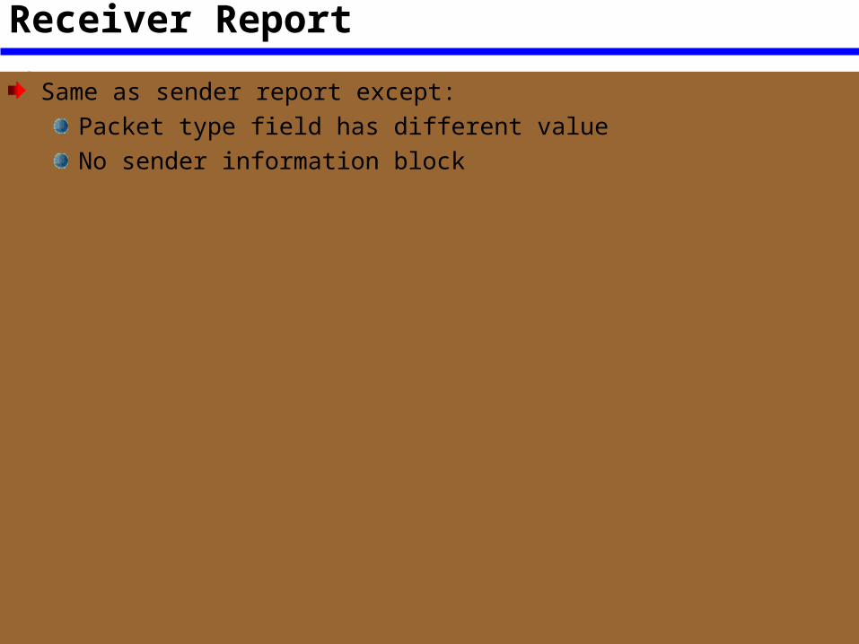
Receiver Report

Same as sender report except:Packet type field has different valueNo sender information block

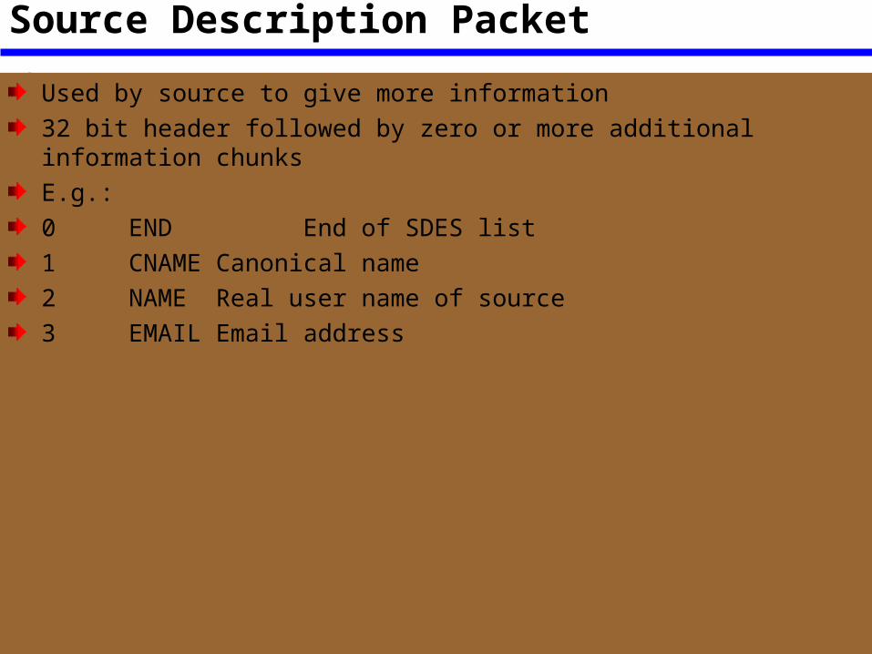
Source Description Packet

Used by source to give more information32 bit header followed by zero or more additional information chunksE.g.:0 END End of SDES list1 CNAME Canonical name2 NAME Real user name of source3 EMAIL Email address

Goodbye (BYE)

Indicates one or more sources no linger activeConfirms departure rather than failure of network

Application Defined Packet

Experimental useFor functions & features that are application specific

Required Reading

Stallings chapter 10