Embed Size (px)
Citation preview

Introduction & motivation Example discussion Hands-on experience
Unit conversion in LBM
Timm Kruger
Department of Microstructure Physics and Metal Forming40237 Dusseldorf, [email protected]
LBM Workshop (Edmonton, Canada), August 22–26, 2011
Max-Planck-Institut fur Eisenforschung, Dusseldorf, Germany Unit conversion in LBM 1 / 31

Introduction & motivation Example discussion Hands-on experience
Outline
1 Introduction & motivation
2 Example discussion
3 Hands-on experience
Max-Planck-Institut fur Eisenforschung, Dusseldorf, Germany Unit conversion in LBM 2 / 31

Introduction & motivation Example discussion Hands-on experience
Outline
1 Introduction & motivation
2 Example discussion
3 Hands-on experience
Max-Planck-Institut fur Eisenforschung, Dusseldorf, Germany Unit conversion in LBM 3 / 31

Introduction & motivation Example discussion Hands-on experience
Physical observables and units
physical observablesusually dimensional, i.e., a number plusa dimensionmeasuring means comparing with areference scale (e.g., measuring tape)
physical unitsfundamental units, e.g., meter, second,kilogram (SI)uniquely derived units, e.g., newton,joule, watt
bethlehem-news.de
Max-Planck-Institut fur Eisenforschung, Dusseldorf, Germany Unit conversion in LBM 4 / 31

Introduction & motivation Example discussion Hands-on experience
Computers and physical units
computers can only process binarynumbersnumbers are dimensionlessuser has to provide unit conversion(physical unit↔ number)
img.ehowcdn.com
proper unit conversions are required to1 set up a computer simulation2 interpret the results afterwards
Max-Planck-Institut fur Eisenforschung, Dusseldorf, Germany Unit conversion in LBM 5 / 31

Introduction & motivation Example discussion Hands-on experience
Hydrodynamics and the law of similarity (1)
dimensionless Navier-Stokes equations
ρ
(∂u∂t
+ (u · ∇)u)
= −∇p + ρν∇2u
∂u∂ t
+ (u · ∇)u = −∇p +1
Re∇2u
u = u/um, p = p/(ρu2m), t = tum/H, ∇ = ∇H, Re =
umHν
significance of Reynolds numberonly dimensionless number constructible from um, H, and νcharacterizes solutions of Navier-Stokes equationsflows with same Re are equivalent, even if um, H, and νare different
Max-Planck-Institut fur Eisenforschung, Dusseldorf, Germany Unit conversion in LBM 6 / 31

Introduction & motivation Example discussion Hands-on experience
Hydrodynamics and the law of similarity (2)
concept of characteristic dimensionless numbers can begeneralized to more complicated hydrodynamic problemsexample: presence of diffusive tracer with diffusivity Dadditional dimensionless number (Schmidt number):Sc = ν/Dflows with same Re and Sc are equivalent
general recommended approachalways find all independent dimensionless numbers for given
problem before anything else is done
Max-Planck-Institut fur Eisenforschung, Dusseldorf, Germany Unit conversion in LBM 7 / 31

Introduction & motivation Example discussion Hands-on experience
Conversion principle (1)
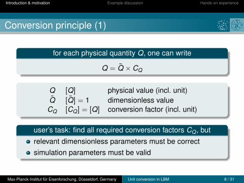
for each physical quantity Q, one can write
Q = Q × CQ
Q [Q] physical value (incl. unit)Q [Q] = 1 dimensionless valueCQ [CQ] = [Q] conversion factor (incl. unit)
user’s task: find all required conversion factors CQ, but
relevant dimensionless parameters must be correctsimulation parameters must be valid
Max-Planck-Institut fur Eisenforschung, Dusseldorf, Germany Unit conversion in LBM 8 / 31
Introduction & motivation Example discussion Hands-on experience
Conversion principle (1)
for each physical quantity Q, one can write
Q = Q × CQ
Q [Q] physical value (incl. unit)Q [Q] = 1 dimensionless valueCQ [CQ] = [Q] conversion factor (incl. unit)
user’s task: find all required conversion factors CQ, but
relevant dimensionless parameters must be correctsimulation parameters must be valid
Max-Planck-Institut fur Eisenforschung, Dusseldorf, Germany Unit conversion in LBM 8 / 31

Introduction & motivation Example discussion Hands-on experience
Conversion principle (2)
example for velocity conversion
u = u × Cu
u = 10 ms , u = 0.1 =⇒ Cu = 100 m
s
conversion of dimensionless numbersdimensionless numbers should generally be invariant, e.g.,
Re = Re ⇐⇒ CRe!
= 1
possible exceptions: e.g., Mach number (next slide).
Max-Planck-Institut fur Eisenforschung, Dusseldorf, Germany Unit conversion in LBM 9 / 31

Introduction & motivation Example discussion Hands-on experience
LBM and the Mach number
usually, LBM Mach number is largerthan in realityotherwise, simulations would be tooexpensive (too many time steps)no problem since Ma is not important
Ma!� 1, e.g., Ma < 0.3
www.allmystery.de
Max-Planck-Institut fur Eisenforschung, Dusseldorf, Germany Unit conversion in LBM 10 / 31

Introduction & motivation Example discussion Hands-on experience
Approaching a hydrodynamic problem
1 identify relevant dimensionless numbers(e.g., Reynolds or Peclet number)
2 write down their definitions,e.g., Re = uH
ν
3 make use of their invariance during unit conversion,e.g., Re = Re and CRe = 1
4 from this, it is possible to construct a unique set of unitconversions
Explicit examples will be shown later!
Max-Planck-Institut fur Eisenforschung, Dusseldorf, Germany Unit conversion in LBM 11 / 31
Introduction & motivation Example discussion Hands-on experience
Primary conversion factors
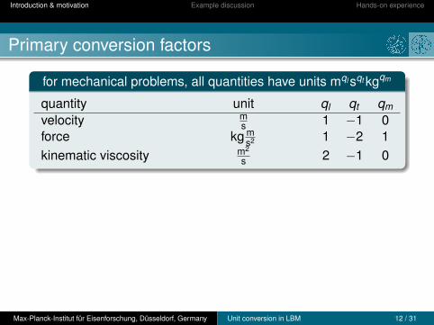
for mechanical problems, all quantities have units mql sqt kgqm
quantity unit ql qt qmvelocity m
s 1 −1 0force kg m
s2 1 −2 1kinematic viscosity m2
s 2 −1 0
three independent primary conversion factors required, e.g., forlength, time, masslength, velocity, energylength, time, density
All other (secondary) conversion factors are uniquely derived.
Max-Planck-Institut fur Eisenforschung, Dusseldorf, Germany Unit conversion in LBM 12 / 31

Introduction & motivation Example discussion Hands-on experience
Primary conversion factors
for mechanical problems, all quantities have units mql sqt kgqm
quantity unit ql qt qmvelocity m
s 1 −1 0force kg m
s2 1 −2 1kinematic viscosity m2
s 2 −1 0
three independent primary conversion factors required, e.g., forlength, time, masslength, velocity, energylength, time, density
All other (secondary) conversion factors are uniquely derived.
Max-Planck-Institut fur Eisenforschung, Dusseldorf, Germany Unit conversion in LBM 12 / 31

Introduction & motivation Example discussion Hands-on experience
Finding secondary conversion factors
1 set primary conversion factors,e.g., for length, time, and density (Cl , Ct , Cρ)
2 express secondary units in terms of primary units,e.g., for the energy
[E ] =kg m2
s2 =kgm3
m5
s2 =[ρ][l]5
[t ]2=
[Cρ][Cl ]5
[Ct ]2
3 read off secondary conversion factor, e.g., for the energy
CE =CρC5
l
C2t
Only the unit of the secondary quantity has to be known!
Max-Planck-Institut fur Eisenforschung, Dusseldorf, Germany Unit conversion in LBM 13 / 31

Introduction & motivation Example discussion Hands-on experience
Outline
1 Introduction & motivation
2 Example discussion
3 Hands-on experience
Max-Planck-Institut fur Eisenforschung, Dusseldorf, Germany Unit conversion in LBM 14 / 31

Introduction & motivation Example discussion Hands-on experience
Gravity-driven planar Poiseuille flow
relevant input parameters
channel height (wall distance) Hviscosity νdensity ρgravity (force per volume) f = ρg
relevant output parametersmaximum velocity(Poiseuille law): Reynolds number:
um =fH2
8ρν Re :=umHν
=gH3
8ν2
H
ρ, ν
gum
Max-Planck-Institut fur Eisenforschung, Dusseldorf, Germany Unit conversion in LBM 15 / 31
Introduction & motivation Example discussion Hands-on experience
Physical parameters
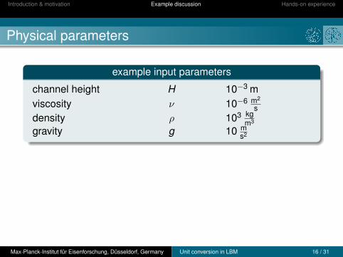
example input parameters
channel height H 10−3 mviscosity ν 10−6 m2
sdensity ρ 103 kg
m3
gravity g 10 ms2
resulting output parameters
um = 1.25 ms , Re = 1250
These values are defined by the physical problem!
Max-Planck-Institut fur Eisenforschung, Dusseldorf, Germany Unit conversion in LBM 16 / 31
Introduction & motivation Example discussion Hands-on experience
Physical parameters
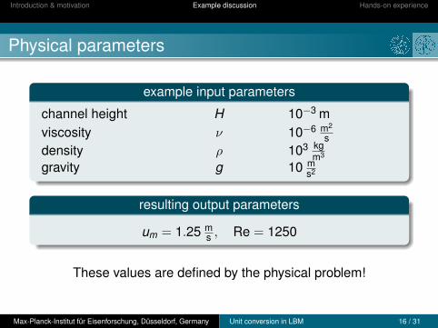
example input parameters
channel height H 10−3 mviscosity ν 10−6 m2
sdensity ρ 103 kg
m3
gravity g 10 ms2
resulting output parameters
um = 1.25 ms , Re = 1250
These values are defined by the physical problem!
Max-Planck-Institut fur Eisenforschung, Dusseldorf, Germany Unit conversion in LBM 16 / 31

Introduction & motivation Example discussion Hands-on experience
Choose simulation parameters
resolution
H = 20, H = 10−3 m =⇒ CH = 5× 10⁻⁵ m
density
ρ = 1, ρ = 103 kgm3 =⇒ Cρ = 103 kg
m3
relaxation time
τ = 0.6
The user may choose any other set of parameters!
Max-Planck-Institut fur Eisenforschung, Dusseldorf, Germany Unit conversion in LBM 17 / 31

Introduction & motivation Example discussion Hands-on experience
Make use of Reynolds number
Reynolds number in physical and dimensionless systems
Re =umHν
, Re =umHν
equality of Reynolds numbers
Re != Re =⇒ ν
ν=
um
um
HH
=⇒ Cν = CuCH
consistency check
[Cν ] = [Cu][CH ] =m2
sX
Max-Planck-Institut fur Eisenforschung, Dusseldorf, Germany Unit conversion in LBM 18 / 31

Introduction & motivation Example discussion Hands-on experience
Get time conversion factor
lattice spacing and time step
for convenience, choose ∆x = 1 and ∆t = 1
=⇒ ∆x = CH , ∆t = Ct
LBM viscosity
ν =
(τ − 1
2
)c2
s ∆t , c2s =
13
∆x2
∆t2 =⇒ ν =τ − 1
23︸ ︷︷ ︸ν
C2H
Ct
time conversion factor
Ct =τ − 1
23
C2Hν
= 8.3× 10⁻⁵ s
Max-Planck-Institut fur Eisenforschung, Dusseldorf, Germany Unit conversion in LBM 19 / 31

Introduction & motivation Example discussion Hands-on experience
Get velocity conversion factor
secondary conversion factor
[u] =[H]
[t ]=⇒ Cu =
CH
Ct=⇒ Cu = 0.6 m
s
compute maximum lattice velocity
um = um/Cu =⇒ um = 2.083
consistency of Reynolds number
Re =umHν
!=
umHν
= 1250 X
Max-Planck-Institut fur Eisenforschung, Dusseldorf, Germany Unit conversion in LBM 20 / 31

Introduction & motivation Example discussion Hands-on experience
Correct simulation parameters
problemSimulation parameters are consistent,
but not valid for LBM simulations (um � 0.3).
correction approach
Cu =CH
Ct=
3τ − 1
2
ν
CH
decrease CH =⇒ more expensivedecrease τ =⇒ LBM may become unstable
User has to find a consistent and valid set of parameters!
Max-Planck-Institut fur Eisenforschung, Dusseldorf, Germany Unit conversion in LBM 21 / 31

Introduction & motivation Example discussion Hands-on experience
Example correction
change resolution and relaxation parameter
CH = 5× 10⁻⁵ m→ C∗H = 1× 10⁻⁵ mτ = 0.6→ τ∗ = 0.55
corrected velocity conversion factor
C∗u =3
τ∗ − 12
ν
C∗H= 6 m
s =⇒ u∗m = 0.2083 X
consistency of Reynolds number
Re =umHν
!=
u∗mH∗
ν∗= 1250 X
The user has found a consistent and valid parameter set.
Max-Planck-Institut fur Eisenforschung, Dusseldorf, Germany Unit conversion in LBM 22 / 31

Introduction & motivation Example discussion Hands-on experience
Get force conversion factor
secondary conversion factor
[f ] =[ρ][H]
[t ]2=⇒ Cf =
CρCH
C2t
=⇒ Cf = 3.6× 10⁹ Nm3
compute lattice force density
f = f/Cf =⇒ f = 2.7× 10⁻⁶
Everything for a successful simulation is prepared!
Max-Planck-Institut fur Eisenforschung, Dusseldorf, Germany Unit conversion in LBM 23 / 31

Introduction & motivation Example discussion Hands-on experience
Alternative routes
start with H and um
1 choose H and um =⇒ CH , Cu
2 find viscosity conversion factor Cν = C2H/Ct =⇒ ν
3 identify relaxation time τ from ν = (τ − 12 )/3
4 find remaining conversion factors & check validity
start with um and τ
1 choose um and τ =⇒ Cu , ν2 find viscosity conversion factor Cν from ν
3 find length conversion factor CH = Cν/Cu =⇒ H4 find remaining conversion factors & check validity
and so on. . .
Max-Planck-Institut fur Eisenforschung, Dusseldorf, Germany Unit conversion in LBM 24 / 31

Introduction & motivation Example discussion Hands-on experience
Outline
1 Introduction & motivation
2 Example discussion
3 Hands-on experience
Max-Planck-Institut fur Eisenforschung, Dusseldorf, Germany Unit conversion in LBM 25 / 31

Introduction & motivation Example discussion Hands-on experience
Gravity-driven Poiseuille flow with diffusive tracer
relevant input parameters
channel height (wall distance) Hviscosity νtracer diffusivity Ddensity ρgravity (force per volume) f = ρg
relevant dimensionless parameters
Reynolds number: Schmidt number:
Re :=umHν
=gH3
8ν2 Sc :=ν
D
H
ρ, ν, D
gum
Max-Planck-Institut fur Eisenforschung, Dusseldorf, Germany Unit conversion in LBM 26 / 31

Introduction & motivation Example discussion Hands-on experience
Formulary
dimensionless parameters
Re =umHν
=gH3
8ν2 , Sc =ν
D
dimensionless viscosity and diffusivity
ν =τν − 1
23
, D =τD − 1
23
gravity
f = ρg
Max-Planck-Institut fur Eisenforschung, Dusseldorf, Germany Unit conversion in LBM 27 / 31

Introduction & motivation Example discussion Hands-on experience
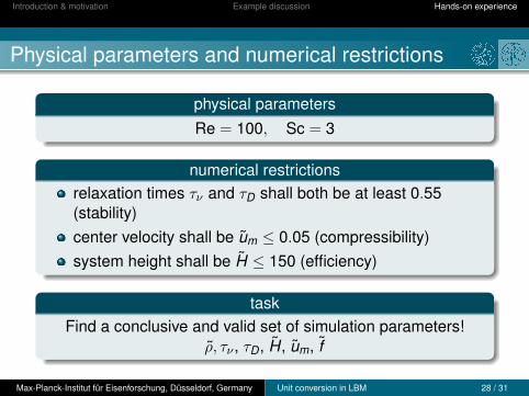
Physical parameters and numerical restrictions
physical parametersRe = 100, Sc = 3
numerical restrictionsrelaxation times τν and τD shall both be at least 0.55(stability)center velocity shall be um ≤ 0.05 (compressibility)system height shall be H ≤ 150 (efficiency)
taskFind a conclusive and valid set of simulation parameters!
ρ, τν , τD, H, um, f
Max-Planck-Institut fur Eisenforschung, Dusseldorf, Germany Unit conversion in LBM 28 / 31

Introduction & motivation Example discussion Hands-on experience
Physical parameters and numerical restrictions
physical parametersRe = 100, Sc = 3
numerical restrictionsrelaxation times τν and τD shall both be at least 0.55(stability)center velocity shall be um ≤ 0.05 (compressibility)system height shall be H ≤ 150 (efficiency)
taskFind a conclusive and valid set of simulation parameters!
ρ, τν , τD, H, um, f
Max-Planck-Institut fur Eisenforschung, Dusseldorf, Germany Unit conversion in LBM 28 / 31

Introduction & motivation Example discussion Hands-on experience
Example solution, part 1
identify minimum relaxation parameters
Sc =ν
D=⇒ Sc =
τν − 12
τD − 12
=⇒ τν = Sc(τD − 0.5) + 0.5
τD,min = 0.55, Sc = 3 =⇒ τν,min = 0.65
identify minimum resolution
Re =umHν
=⇒ H = Reτν − 0.5
3um
τν,min = 0.65, um,max = 0.05, Re = 100 =⇒ Hmin = 100
Max-Planck-Institut fur Eisenforschung, Dusseldorf, Germany Unit conversion in LBM 29 / 31

Introduction & motivation Example discussion Hands-on experience
Example solution, part 2
chosen set of simulation parameters
τν = 0.65, τD = 0.55, H = 100, um = 0.05
validity and consistency already assured
Re =umHν
= 100, Sc =ν
D= 3 X
set densityρ = 1 (arbitrary)
set gravity
Re =gH3
8ν2 =⇒ f = ρg =8ρν2
H3Re = 2× 10⁻⁶
Max-Planck-Institut fur Eisenforschung, Dusseldorf, Germany Unit conversion in LBM 30 / 31

Introduction & motivation Example discussion Hands-on experience
Further comments
systems with identical Re and Sc are equivalent=⇒ no explicit conversion factors required at this point!scale can be introduced afterwards, e.g.,
H = 10−3 m =⇒ CH = 10−5 m
all other conversion factors are then obtained as in theexample discussion
Max-Planck-Institut fur Eisenforschung, Dusseldorf, Germany Unit conversion in LBM 31 / 31