Unit 5 : Day 1 : Continuous Data MDM4U Description ...edugains.ca/resources/LearningMaterials/TIPS/tips4rm/mdm4u/Unit5... · MDM 4U: Unit 5 – Modeling Continuous Data (Draft –

MDM 4U: Unit 5 – Modeling Continuous Data (Draft – Fall 2007) 1

Unit 5 : Day 1 : Continuous Data MDM4U Minds On: 10

Action: 55

Consolidate:10

Total=75 min

Description/Learning Goals • Contrast discrete data and continuous data • Describe the shape of frequency histograms for continuous data (e.g., skewed-

left, skewed-right, bimodal, symmetric) • Use the mean, median and standard deviation to help classify the different

shapes of frequency histograms of continuous data

Materials • BLM 5.1.1 – 5.1.6 • Data projector • Video clips

“Slideshow” and “Movie”

• Graphing calcs • Computer lab

Assessment Opportunities

Minds On… Whole Class Don’t Judge Too Early Watch video clip “Slideshow” and attempt to explain what has happened based on the information provided. Now watch the video clip “Movie”. Does the story you deduced from the slides match the real story from the movie? Students use BLM 5.1.1 to guide them through this exploration on continuous versus discrete data sets. Mathematical Process Focus: Reflecting - students will reflect on what they thought was happening in the video vs. what actually happened and compare that to the difference between continuous and discrete data. Ensure students have correct definitions for descrete and continuous data Review mean, median, mode and standard deviation

Action! Whole Class/Small Groups Exploration Using BLM 5.1.2 and an overhead projector discuss the differences seen in the 4 different histograms. Have students label each histogram as being skewed-left, skewed-right, bimodal, or symmetric. In small groups have students develop a list of situations in which the data would produce the 4 different histograms. Mathematical Process Focus: Connecting –students will connect histogram shapes to real life situation that could produce them. Pairs Investigation Distribute BLM 5.1.3 to pairs and have students determine the mean, median, mode and standard deviation of each data set. Using technology (e.g. graphing calc, Excel, Fathom ...) have the students graph each data set and instruct them to summarize their findings.

Connecting/Observation/Mental Note: Observe individuals as they work in small groups. Listen to discussions between students as they consolidate their understanding of the observations they made from the exploration.

Consolidate Debrief

Whole Class Discussion As a class summarize students findings using BLM 5.1.4.

Application Concept Practice

Home Activity or Further Classroom Consolidation Complete BLM 5.1.5 and BLM 5.1.6. Note BLM 5.1.6 MUST be completed for tomorrow as we will be using it in the lesson.


5.1.1: Don’t Judge Too Soon MDM4U Take a look at the series of slides in the video clip “Slideshow” and attempt to determine what has happened based on the information provided to you. 1. Write a description frame by frame of what you think is happening in this apartment. 2. Watch the movie in the video clip “Movie” and write a description of what actually

happened in the apartment. 3. Did the story you deduced from the slides match the actual story in the movie?

Which provides more information? Mathematicians attempt to interpret events and processes that occur based on the data available to them. The more data that can be collected to fill in the unknown gaps, the more accurately the mathematician or scientist can interpret the story. Discrete data: Continouous data:


5.1.2: Continuous Data Histograms MDM4U

________________________________ ____________________________

______________________________ _______________________________


5.1.2: Classifying Frequency Histograms – Teacher notes Skewed-Right

Mean> Median> Mode Skewed-Left

Mean< Median< Mode

Symmetric

Mean= Median= Mode Bimodal

2 modes


5.1.3: Classification of Histograms MDM4U

Using the following data sets calculate the mean, median, mode, and standard deviation. Graph each data set on the grids provided. Label the shape of each graph. Compare your graphs to your measures of central tendency and summarize your findings. 1) Marks on a project {1, 2, 3, 4, 3, 3, 4, 3, 2, 3, 3, 2, 3, 2, 1, 2, 3, 4, 3, 3, 2, 3, 2, 3, 2, 3} 2) Monthly rent ($) { 625, 750, 800, 650, 725, 1250, 625, 650, 850, 625} 3) Drive thru times (min) {5, 5.5, 6.5, 7, 7.5, 7, 7, 5, 6.5, 5, 5, 8.5, 0.5, 4.5, 7} 4) Age of cousins {12, 15, 8, 12, 15, 10, 3, 14, 15} 1) Marks on a project

Shape_____________ Mean__________ Mode___________ Median_________ Standard Deviation_______ Summary________________________________________________________ ________________________________

2) Monthly rent

Shape_______________ Mean__________ Mode___________ Median__________ Standard Deviation_______ Summary________________________________________________________________________________________

3) Monthly rent Shape____________ Mean__________ Mode___________ Median__________ Standard Deviation ______ Summary ________________________ ________________________________________________________________

4) Age of cousins Shape_______________ Mean__________ Mode___________ Median__________ Standard Deviation_______ Summary________________________________________________________________________________________


5.1.4:Classifying Frequency Histograms Practice MDM4U 1) Identify each of the following situations as discrete distributions or continuous distributions.

Explain your reasoning.

a) counting the number of outcomes for drawing a card b) measuring the time taken to complete a task c) counting the number of outcomes when tossing three coins d) measuring the maximum distance a ball can be thrown

2) Using the mean, median and mode, describe the shape of the frequency histogram.

a) mean: 7.5 median: 6 mode: 5.7 b) mean: 6 median: 6 mode: 10, 12 c) mean: 7.5 median: 8.5 mode: 9 d) mean: 7.5 median: 7.5 mode: 7.5

3) A pair of dice are rolled numerous times. The sum of the dice, as well as the frequency, is

recorded. Calculate the mean, median, mode, and standard deviation. Use these results to identify the shape of this histogram.

Sum 2 3 4 5 6 7 8 9 10 11 12 Frequency 2 3 5 7 9 11 8 7 4 2 1


5.1.5: Distribution of Data Assignment MDM4U The general shape of a frequency distribution (histogram or frequency polygon) can typically be categorized in one of four ways. i) U-Shaped Distribution ii) Uniform Distribution iii) Mound-Shaped Distributions iv) Skewed Distributions ACTIVITY: Using a spreadsheet program create frequency histograms for the following groups of data taken from a variety of real life situations. Copy and Paste the graphs into a word processing document. Below each graph state which category the distribution of the data falls into. Explain. Also, draw a smooth, continuous curve representing the general shape of the distribution. Dice Sums Sum 2 3 4 5 6 7 8 9 10 11 12 Frequency 1 2 3 4 5 8 6 3 2 1 0 Simple Dice Game Score 1 2 3 4 5 6 Frequency 18 17 18 18 16 19 Spider Solitaire Score 400-449 450-499 500-549 550-599 600-659 650-699 700-749 750-799 800-849

Frequency 15 10 6 4 0 4 6 10 15 Solitaire Score 0-19 20-39 40-59 60-79 80-99 100-119 120-139 140-159 Frequency 20 15 12 7 5 2 1 1


Unit 5 : Day 2 : Continuous Data MDM4U Minds On: 20

Action: 40

Consolidate:15

Total=75 min

Description/Learning Goals • By increasing the number of intervals of a frequency histogram, postulate the

shape of the probability distribution for the continuous random variable • Recognize that the probability of a continuous random variable taking any

specific value is zero

Materials • Computer lab

with Fathom • BLM 5.2.1


Minds On… Small Groups/Paris Peer Evaluation In small groups or pairs have students peer evaluate each others assignment BLM 5.1.5. Students should not be given the answers, they are to discuss and compare their work. Once each group comes to a general consensus on the correct answers the assignment may be taken up as a class.

Whole Class Discussion Have each group or pair present the answer to one question from the assignment.

Action! Individual Investigation Using BLM 5.2.1 students investigate how increasing or decreasing the number of intervals of a frequency histogram alters the shape of the probability distribution for the random continuous variable. They also recognize that the probability of a continuous random variable taking any specific value is zero and that probabilities must be calculated over an interval (i.e., the probability of students heights being between 166-170cm) Process Expectations/ Observation/ Mental Note: Observe individuals as they work through the investigation. Listen to discussions between students as they consolidate their understanding of the observations they have made through this investigation. Mathematical process focus: reflecting – students will reflect on how histograms are altered by changing intervals

Consolidate Debrief

Whole Class Discussion As a class have the students use their summaries from their investigation to create a class summary. This should be teacher oriented but student fed.

Reflection

Home Activity or Further Classroom Consolidation Write a journal entry outlining the key concepts you have learned within yesterday and today’s lesson. Include real life examples of when and where these concepts are used.


5.2.1: Interval Investigation on Continuous Data MDM4U

PART A: Investigation using graph paper

1) Use the following data to complete the frequency table below.

Table 1. Height of High School Students in cm 145 155 147 157 148 165 167 195 168 201 172 173 163 160 155 159 163 167 182 195 176 178 164 179 182 165 143 142 149 152 151 168 186 195 154 165 187 195 203 202 154 198 165 172 183 185 188 192 172 196 174 154 152 163 175 179 184 165 135 174 185 165 140 135 196 210 165 178 185 135 175 195 145 168 175 172 173 186 173 173 173 186 165 185 178 159 165 148 195 148 165 163 161 160 150 153 158 167 196 185 172 148 159 165 135 180 196 205 165 203

Table 2. Frequency table Interval Ranges Tally Frequency 131-135 136-140 141-145 146-150 151-155 156-160 161-165 166-170 171-175 176-180 181-185 186-190 191-195 196-200 201-205 206-210 211-215

2) Use table 2 and create a frequency histogram and a frequency polygon (approximates the frequency distribution) on graph paper.

3) Describe the shape of these graphs. 4) Decrease the number of intervals by grouping them together in ranges of 25 i.e., 125-149, 150-174 and so on. Using the new frequencies and interval ranges graph a frequency histogram and a frequency polygon on a separate piece of graph paper.


5.2.1: Interval Investigation on Continuous Data(continued) MDM4U

5) Describe the shape of these graphs. 6) What do you notice has happened to the graphs by changing the number of intervals?

PART B: Investigation using technology

1) Create a histogram in fathom using the data from table 1 in part A. 2) What is the interval of your bars in your histogram_____________________? 3) How would you describe the shape of this histogram

4) Place your curser between two of the histogram bars and increase the size of the

interval of the bars, thus decreasing the number of intervals overall. Change your x- and y-axis so that the entire histogram is visible if necessary. How would you now describe the shape of this histogram

5) Now decrease the size of the intervals bars, thus increasing the number of intervals

overall. How would you describe the shape of this histogram. 6) Create your own or find a random continuous data set. Make a frequency table using

your data set and an appropriate interval range. Create a frequency histogram and frequency polygon using your frequency table. Now repeat part B and create 10 different histograms by altering the number of intervals. Your data set must contain a minimum of 50 data points.

7) In two or three sentences summarize your findings on how increasing and or decreasing

the intervals of a frequency histogram alters the shape of the probability distribution for the continuous random variable.


5.2.1:Interval Investigation on Continuous Data(continued) MDM4U Part C: Investigating probability 1) Using the frequency histogram you graphed in part A #2 determine the probability of a student being 161 cm tall. 2) What is the probability of a student being 178 cm tall? 3) What is the probability of a student being 199 cm tall? 4) What do you notice about the probabilities of these individual heights? What do you think would be a better way to calculate probabilities for continuous random data? 5) Calculate the probability that the students heights are within the interval range of 156-160? What about between the interval range of 171-175? 6) Summarize your findings by explaining how to calculate probabilities using continuous random data.


Unit 5 : Day 3 : Characteristics of the Normal Distribution MDM4U Minds On: 10

Action: 45

Consolidate:20 Total=75 min

Description/Learning Goals • Recognize important features of a normally distributed data (e.g. bell-

shaped, the percentages of data values within one, two and three standard deviations of the mean, mean and median are equal, symmetric about mean)

• Recognize and describe situations that might be normally distributed.

Materials • Computer with

data projector • Simulation -FTM

5.3.1 • BLM 5.3.1- 5.3.4


Minds On… Pairs Activity Provide each student with a cut out copy of BLM 5.3.1. In pairs the students group similar histograms together. They should determine what criteria they used for the groupings.

Whole Class Discussion Engage students in a discussion about the various distributions with emphasis on the bell-shaped (approximately Normally distributed) distributions and discuss the common characteristics of these bell-shaped curves. Summarize this discussion in a board note.

Action! Whole Class Guided Investigation After the discussion of the characteristic shape of normal distributions use the Fathom™ simulation FTM 5.3.1 to investigate the affect on the shape of the curve by changing the mean and standard deviation. Instruct students to record and summarize their observations. Individual/Sharing Investigation Using BLM 5.3.2 students investigate and determine the approximate percentage of data that lie within 1, 2, and 3 standard deviations of the mean (68%, 95%, 99.7% rule). Students share their observations and results with other students in the classroom to see if they have matching results. Use BLM 5.3.3 to consolidate students’ learning. Process Expectations/Investigation/Observation: Listen to discussions between students as they consolidate their understanding of the observations they made from the investigation. Mathematical Process Focus: Selecting Tools – students will learn how to select appropriate tools for calculations.

Consolidate Debrief

Whole Class Summary Note Students write a brief summary of their findings; what factors affect the shape of a normal distribution and what empirical rules about probabilities can be determined? Also, since the values are only approximate, limitations of the investigation should be discussed in the summary note with a detailed diagram. Then solve the following example with them: Example: The mass of 17 year olds in a data management course is normally distributed. The mean is 65 kg and the standard deviation is 5 kg. a) Sketch the curve including the mean, and standard deviation intervals. b) Determine the probability that a student in the class has a mass between

60kg and 65kg. P( 60 < X < 65) c) Determine the probability that a student in the class has a mass greater

than 75kg. P( X > 75)

. Percentages are found by counting the squares under the curve between each of the standard deviations indicated. Have students draw solid lines at !± , 2!± , and 3!± .

This will allow them to count the number of squares in each region more clearly.

Application Concept Practice

Home Activity Complete BLM 5.3.4


5.3.1: What’s Normal? MDM4U

1

2

3

4

5

6

�

Graph_A-2 0 2 4 6 8 10 12

Histogram

2

4

6

8

10

�

Graph_B0 2 4 6 8 10

Histogram

1

2

3

4

5

6

�

Graph_C0 2 4 6 8 10 12

Histogram

1

2

3

4

5

6

�

Graph_D0 2 4 6 8 10 12

Histogram

2

4

6

8

10

12

14

�

Graph_E0 2 4 6 8 10 12

Histogram

2468101214161820

�

Graph_F0 2 4 6 8 10 12 14

Histogram


5.3.1: What’s My Normal? (continued) MDM4U

2

4

6

8

10

12

�

Graph_G0 2 4 6 8 10 12

Histogram

2

4

6

8

10

12

14

16

�

Graph_H-2 0 2 4 6 8 10 12

Histogram

2

4

6

8

10

12

�

Graph_I0 2 4 6 8 10 12

Histogram

2

4

6

8

10

12

�

Graph_J0 2 4 6 8 10 12

Histogram

2

4

6

8

10

12

�

Graph_K0 2 4 6 8 10 12

Histogram

2

4

6

8

10

12

�

Graph_L0 2 4 6 8 10 12

Histogram


5.3.2: Features of the Normal Distribution MDM4U

µ = 2! =

µ = 5! =

Total number of squares under the curve: ________

Number of squares ± 1 Std. Dev of mean: _______ Fraction of Total: ________

Number of squares ± 2 Std. Dev of mean: _______ Fraction of Total: ________ Number of squares ± 3 Std. Dev of mean: _______ Fraction of Total: ________

Total number of squares under the curve: ________

Number of squares ± 1 Std. Dev of mean: _______ Fraction of Total: ________

Number of squares ± 2 Std. Dev of mean: _______ Fraction of Total: ________ Number of squares ± 3 Std. Dev of mean: _______ Fraction of Total: ________

Summarize Your Observations: What do you notice about the number of squares under the curve for each distribution? Write a rule for the percentage of data points within 1, 2 and 3 standard deviations of the mean.


5.3.3: 68%,95%,99.7% Rule MDM4U For any given normal distribution X, the percentage of data; • between µ !" and µ !+ is approximately 68%. (i.e. within one standard deviation of the

mean.) • between 2µ !" and 2µ !+ is approximately 95% • between 3µ !" and 3µ !+ is approximately 99.7%

µ µ !+ 2µ !+ 3µ !+3µ !" 2µ !" µ !"

68%

95%

99.7%


5.3.4: Normal Distribution Practice MDM4U

1. Name the following distributions. a. b.

2468101214

�

Heights_of_Trees0 1 2 3 4 5 6 7 8

Histogram

_______________________ ____________________

2. Sally is 164 cm tall. In her school, the girls heights are normally distributed with a mean of 168cm and a standard deviation of 4cm. a. What is the probability that Sally’s friend Joanne is taller than she is? b. What is the probability that Joanne is between 164cm and 172cm tall?

3. The daily sales of Gary’s chip truck has a mean of $675.00 and a standard deviation of

$35.50. a. What percent of time will the daily sales be greater than $639.50? b. What percent of time will the daily sales be less than $746.00?

4. The mean household income in Kingston is $45000 with a standard deviation of $15000.

Household incomes below $30000 will receive a tax credit, household incomes between $30000 and $75000 will have to pay a 2% tax, and household incomes over $75000 will have to pay a 5% tax. a. What percentage of households will have to pay a 2% tax b. What percentage of households will not have to pay tax c. What percentage of households will pay tax.

5. An elite university only accepts the top 5% of students within the province to attend their

university. Last year the student’s average marks were normally distributed with a mean of 75% and a standard deviation of 7.5%. What average is needed in order to attend this university?

2

4

6

8

10

12

�

Hours_of_Study_for_Exams0 10 20 30 40

Histogram


Unit 5 : Day 4 : Binomial and Hypergeometric Distributions MDM4U Minds On: 15

Action: 50


Description/Learning Goals • Investigate the conditions under which the shape of a binomial distribution

approaches a normal distribution • Investigate the conditions under which the shape of a hypergeometric

distribution approaches a normal distribution

Materials • Graphing

calculators, • BLM 5.4.1, -

5.4.2


Minds On… Whole Class Discussion As a class determine whether each situation below can be modelled by a binomial distribution or a hypergeometric distribution.

a) A child rolls a die ten times and counts the number of 3s. b) Calculating the probability of a prize being won within the first 3 tries c) A factory producing electric motors has a 0.2% defect rate. A quality-

control inspector needs to determine the expected number of motors that would fail in a day’s production.

d) rolling a die until a 6 shows. e) The faces of a 12-sided die are numbered from 1 to 12. What is the

probability of rolling 9 at least twice in ten tries? f) In a TV game show, the grand prize is randomly hidden behind one of

three doors. On each show, the finalist gets to choose one of the doors. What is the probability that no finalists will win a grand prize on four consecutive shows?

g) Suppose that 1 out of 25 bingo cards gives a prize. What is the probability of winning of the third try.

h) Fifteen percent of the world’s population are left-handed. What is the probability that 50 people within your school are left-handed.

Mathematical Process Focus: Connecting – students will connect the real life situations given to the appropriate distribution type.

Action! Pairs Golfing in Pink and Making the Team Have students complete in pairs, the investigations on BLM 5.4.1 and BLM 5.4.2 using graphing calculators.

Learning Skills/ Observation/ Mental Note: Observe individuals as they work through the investigation. Listen to discussions between students as they consolidate their understanding of the observations they made from the investigation.

Consolidate Debrief

Whole Class Discussion As a class summarize student’s findings at the front of the room. Have students look for the similarities in each others work so that a general summary can be obtain (i.e., for binomial distributions as the number of trials increases and/or the probability of “success” gets closer to one-half and for hypergeometric distributions as the number of dependent trials increases and/or the probability of “success” gets closer to one-half)

Optional: Split the class into two sections, have one section complete BLM 5.4.1 and the other complete BLM 5.4.2 the have students compare results.

Reflection Home Activity Reflect on what you discovered from the investigation by writing a journal entry outlining why this knowledge is needed and where it can be used.


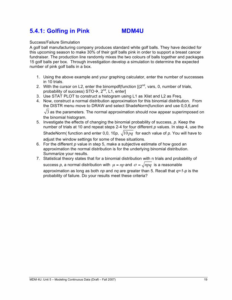
5.4.1: Golfing in Pink MDM4U Success/Failure Simulation A golf ball manufacturing company produces standard white golf balls. They have decided for this upcoming season to make 30% of their golf balls pink in order to support a breast cancer fundraiser. The production line randomly mixes the two colours of balls together and packages 15 golf balls per box. Through investigation develop a simulation to determine the expected number of pink golf balls in a box.

1. Using the above example and your graphing calculator, enter the number of successes in 10 trials.

2. With the cursor on L2, enter the binompdf(function [(2nd, vars, 0, number of trials, probability of success) STO, 2nd, L1, enter]

3. Use STAT PLOT to construct a histogram using L1 as Xlist and L2 as Freq. 4. Now, construct a normal distribution approximation for this binomial distribution. From

the DISTR menu move to DRAW and select ShadeNorm(function and use 0,0,6,and 3 as the parameters. The normal approximation should now appear superimposed on

the binomial histogram. 5. Investigate the effects of changing the binomial probability of success, p. Keep the

number of trials at 10 and repeat steps 2-4 for four different p values. In step 4, use the ShadeNorm( function and enter 0,0, 10p, 10pq for each value of p. You will have to adjust the window settings for some of these situations.

6. For the different p value in step 5, make a subjective estimate of how good an approximation the normal distribution is for the underlying binomial distribution. Summarize your results.

7. Statistical theory states that for a binomial distribution with n trials and probability of success p, a normal distribution with npµ = and npq! = is a reasonable approximation as long as both np and nq are greater than 5. Recall that q=1-p is the probability of failure. Do your results meet these criteria?


5.4.2: Making the Team! MDM4U Choosing a Hockey Team The mayor of Toronto has decided that the city’s population can now host a second NHL team. The coach has hosted try-outs and has cut the possible player list down to 50 players. The coach has to select 22 players from this list of 50 possible players. Suppose that 28 of these 50 players are non-Canadian. Develop a simulation to determine the probability distribution for the number of Canadians selected for this team.

1. Using the above example and your graphing calculator, enter the number of successes

in 10 trials. 2. With the cursor on L2, enter the binompdf(function [(2nd, vars, 0, number of trials,

probability of success) STO, 2nd, L1, enter] 3. Use STAT PLOT to construct a histogram using L1 as Xlist and L2 as Freq. 4. Now, construct a normal distribution approximation for this hypergeometric distribution.

From the DISTR menu move to DRAW and select ShadeNorm(function and use 0,0,6,and 3 as the parameters. The normal approximation should now appear superimposed on the hypergeometric histogram.

5. Investigate the effects of changing the binomial probability of success, p. Keep the number of trials at 10 and repeat steps 2-4 for four different p values. In step 4, use the ShadeNorm( function and enter 0,0, 10p, 10pq for each value of p. You will have to adjust the window settings for some of these situations.

6. For the different p value in step 5, make a subjective estimate of how good an approximation the normal distribution is for the underlying hypergeometric distribution. Summarize your results.


Unit 5 : Day 6 : Probability Distributions & Z-Scores MDM4U Minds On: 30

Action: 40


Description/Learning Goals • Use a discrete probability distribution to approximate the probability that a

normal random variable takes on a specific range of values. • Define and Calculate z-scores

Materials • BLM 5.6.1 • BLM 5.6.2 • metre sticks • Graphing

calculators or computers


Minds On… Whole Class Discussion Write the following on the board:

Z-Scores: How far does data lie from the mean as a multiple of the standard deviation? (i.e. how many standard deviations away from the mean is a given data point?)

Discuss the question as a class and create a board note on calculating Z-scores.

Small Groups Practise Handout BLM 5.6.1 and have students complete the work in pairs. Problem Solving/Observation/Mental Note: Observe students as they work through the basic z-score problems and ask groups questions to check for understanding.

Action! Whole Class Investigation Set-Up Handout BLM 5.6.2 and have students fill in their own data as well as the rest of the classes - this can be done on an overhead to speed up the process. (This can be extended to include additional height data from another class of similar demographics) Pair/Share Investigation Once the class has the data, instruct them to plot a histogram of the data using technology and calculate the mean and standard deviation. Write the following on the board for pairs to discuss and record observation about the data collected:

Is the data approximately normally distributed? Discuss validity of measurements and consequently the calculations. Determine the z-score of your height compared to the mean.

Mathematical Process Focus: Reflecting: Students will reflect on the data and their calculations to answer the above questions.

Learning Skills/Performance Task/Checklist: Observe students as they work through the task. Assess their interaction with one another and their organization.

ConsolidateDebrief

Whole Class Discussion Wrap up the class with a recap of how to calculate z-scores and what they mean in terms of relative distances from the mean.

Application Concept Practice Skill Drill

Home Activity Complete assigned questions on calculating z-scores


5.6.1: Catching Z’s MDM4U 1. Calculate the z-scores for the following data points if the mean for the data set is 6 and the

standard deviation is 2. a) 4 b) 7 c) 1.5

2. A student scores 85% on a data management test. The class average was determined to be 77% with a standard deviation of 3.2%. How many standard deviations from the mean is the students’ score? Is the score above or below the mean?

3. A data set has a mean of 23. Determine the value of the data points corresponding to the

following z-score values a) 0.6 b) 1.5 c) -2.3

4. A given data point in a set of data has a value of 7.3. Determine the mean of the data set if the data point has the following z-score values a) 2.1 c) -1.5

5. Calculate the mean ( µ ) of a data set given the following information about the data point and the standard deviation a) 78x = , 8! = b) 198x = , 23.6! =


5.6.2: Tall Tales MDM4U Student’s Name Height (cm)

Mean_____________ Standard Deviation___________ z-score of your height from the mean_____________


Unit 5: Day 7 : Determining Probabilities from Standard Normal Table MDM4U Minds On: 45

Action: 20


Description/Learning Goals • Read and manipulate probabilities from a table of values of the standard normal

distribution.

Materials • Computers with

internet access • Applet files • BLM 5.7.1 • BLM 5.7.2 • BLM 5.7.3 • BLM 5.6.4


Minds On… Whole Class Discussion/Practice Recap activity from previous day. Discuss results of the data collection. Solve basic probability problems related to height data from previous day leading into more complicated problems. (e.g. What is the probability that student A has a height less than 2! from the mean?) The problems should only make use of the 68, 95, 99.7 rule. Engage the students in a discussion on what happens if the data point in question does not allow you to use the rule.

Whole Class Brainstorm Lead a class in brainstorming on the following question: How can you determine the probabilities from a normally distributed data set if the data point is not exactly on !± , 2!± , and 3!± ?

Individual/Pairs Exploration Students use the applet and BLM 5.7.1 to explore the probabilities for normal distributions.

Action! Whole Class Demonstration/Lesson Introduce The Standard Normal Distribution ( 0µ = , 1! = ) (i.e. transforms ( ) ( )P x X P z Z< ! < )

Introduce The Standard Normal Distribution Table (probabilities have been pre-calculated and can be read from the table – BLM 5.7.2) Solve some sample problems as a class using the Standard Normal Table. On example is given on BLM 5.7.3 Solve some probabilities using the Standard Normal Table using the data that was collected on the previous day. (e.g. Students can calculate the probability that a student chosen at random in their class is shorter than them; taller than them, etc. )

Individual Practise Handout BLM 5.7.4 for students to practise the above skill with. Problem Solving/Performance Task/Scoring Guide: Collect assigned work and assess based on proper notation and problem solving skills. Mathematical Process Focus: Tools & Strategies – students will learn how to use a new tool for solving probability problems.

Consolidate Debrief

Individual Journal Instruct students to summarize the day’s lessons and outcomes in a journal entry.

Visual java applet (online or the applet can be loaded locally): http://www.math.csusb.edu/faculty/stanton/m262/normal_distribution/normal_distribution.html As mentioned previously the normal distribution should be normalized so that the area under the curve is equal to 1. Thus the shaded region between two values (area) represents the probability of a random variable falling inside this range. Drawing a diagram and shading the region in question is a useful strategy help students understand the concept.

Application Concept Practice Skill Drill

Home Activity or Further Classroom Consolidation Complete the assignment questions.


5.7.1: Normal Distribution Exploration MDM4U Normal Distribution Calculator (Java Applet) Recall: the area under the entire bell curve is exactly 1. Therefore any fraction of the curve that is shaded should be a decimal value less than one. This decimal value related to the shaded area under the curve represents the probability that a data value lies between the lowerbound (x1) and upperbound (x2). 1. Load up the applet on your computer. 2. Set the mean to 25 and the standard deviation to 5. Empirical Rule Validation: 3. Set

1x to 20 and

2x to 30. Before calculating; estimate (by shading the area between

1x and

2x )

what the probability, (20 30)P X< < , should be. Check this and record your values. 4. Repeat step 3 using a

i) 1x = 15 and

2x = 35

ii) 1x = 10 and

2x = 40.

iii) 1x = 25 and

2x = 30.

iv) 1x = -1E99 and

2x = 25.

Record your estimates and calculated observations. Were your estimates correct? Calculating Probabilities: What happens if the data values are not exactly positioned at integer multiples of the standard deviation? 5. Keep the same mean and standard deviation. 6. On the graphs provided draw lines corresponding to

1x and

2x ; shade the region between them.

Estimate the probability (i.e. percentage, written as a decimal, of the curve that is filled) and then use the probability calculator to check your values.

1 2( )P x X x< < Lowerbound (

1x ) Upperbound (

2x ) Estimated Calculated

25 37 17 25 10 1E99 30 33 17 22 -1E99 30 21 26 7. Comment on your accuracy by comparing your estimated and calculated values.

8. Shade an area that represents 20% of the area. Estimate the values of 1x and

2x . Check using the

applet calculator. Comment on your accuracy.


5.7.1: Normal Distribution Exploration (Cont) MDM4U

( )P X< <

( )P X< <

( )P X< <

( )P X< <


5.7.2: Standard Normal Distribution Table MDM4U

Standard Normal Distribution

Z 0.00 0.01 0.02 0.03 0.04 0.05 0.06 0.07 0.08 0.09

0.0 0.0000 0.0040 0.0080 0.0120 0.0160 0.0199 0.0239 0.0279 0.0319 0.0359

0.1 0.0398 0.0438 0.0478 0.0517 0.0557 0.0596 0.0636 0.0675 0.0714 0.0753

0.2 0.0793 0.0832 0.0871 0.0910 0.0948 0.0987 0.1026 0.1064 0.1103 0.1141

0.3 0.1179 0.1217 0.1255 0.1293 0.1331 0.1368 0.1406 0.1443 0.1480 0.1517

0.4 0.1554 0.1591 0.1628 0.1664 0.1700 0.1736 0.1772 0.1808 0.1844 0.1879

0.5 0.1915 0.1950 0.1985 0.2019 0.2054 0.2088 0.2123 0.2157 0.2190 0.2224

0.6 0.2257 0.2291 0.2324 0.2357 0.2389 0.2422 0.2454 0.2486 0.2517 0.2549

0.7 0.2580 0.2611 0.2642 0.2673 0.2704 0.2734 0.2764 0.2794 0.2823 0.2852

0.8 0.2881 0.2910 0.2939 0.2967 0.2995 0.3023 0.3051 0.3078 0.3106 0.3133

0.9 0.3159 0.3186 0.3212 0.3238 0.3264 0.3289 0.3315 0.3340 0.3365 0.3389

1.0 0.3413 0.3438 0.3461 0.3485 0.3508 0.3531 0.3554 0.3577 0.3599 0.3621

1.1 0.3643 0.3665 0.3686 0.3708 0.3729 0.3749 0.3770 0.3790 0.3810 0.3830

1.2 0.3849 0.3869 0.3888 0.3907 0.3925 0.3944 0.3962 0.3980 0.3997 0.4015

1.3 0.4032 0.4049 0.4066 0.4082 0.4099 0.4115 0.4131 0.4147 0.4162 0.4177

1.4 0.4192 0.4207 0.4222 0.4236 0.4251 0.4265 0.4279 0.4292 0.4306 0.4319

1.5 0.4332 0.4345 0.4357 0.4370 0.4382 0.4394 0.4406 0.4418 0.4429 0.4441

1.6 0.4452 0.4463 0.4474 0.4484 0.4495 0.4505 0.4515 0.4525 0.4535 0.4545

1.7 0.4554 0.4564 0.4573 0.4582 0.4591 0.4599 0.4608 0.4616 0.4625 0.4633

1.8 0.4641 0.4649 0.4656 0.4664 0.4671 0.4678 0.4686 0.4693 0.4699 0.4706

1.9 0.4713 0.4719 0.4726 0.4732 0.4738 0.4744 0.4750 0.4756 0.4761 0.4767

2.0 0.4772 0.4778 0.4783 0.4788 0.4793 0.4798 0.4803 0.4808 0.4812 0.4817

2.1 0.4821 0.4826 0.4830 0.4834 0.4838 0.4842 0.4846 0.4850 0.4854 0.4857

2.2 0.4861 0.4864 0.4868 0.4871 0.4875 0.4878 0.4881 0.4884 0.4887 0.4890

2.3 0.4893 0.4896 0.4898 0.4901 0.4904 0.4906 0.4909 0.4911 0.4913 0.4916

2.4 0.4918 0.4920 0.4922 0.4925 0.4927 0.4929 0.4931 0.4932 0.4934 0.4936

2.5 0.4938 0.4940 0.4941 0.4943 0.4945 0.4946 0.4948 0.4949 0.4951 0.4952

2.6 0.4953 0.4955 0.4956 0.4957 0.4959 0.4960 0.4961 0.4962 0.4963 0.4964

2.7 0.4965 0.4966 0.4967 0.4968 0.4969 0.4970 0.4971 0.4972 0.4973 0.4974

2.8 0.4974 0.4975 0.4976 0.4977 0.4977 0.4978 0.4979 0.4979 0.4980 0.4981

2.9 0.4981 0.4982 0.4982 0.4983 0.4984 0.4984 0.4985 0.4985 0.4986 0.4986

3.0 0.4987 0.4987 0.4987 0.4988 0.4988 0.4989 0.4989 0.4989 0.4990 0.4990

Probabilities are found between 0 and z. Negative z-scores have the same probability.


55 50.62.3( 55) ( )

( 1.91)

0.972

P x P z

P z

!< = <

" <

"

( 55) ( 55)

1 ( 55)

1 0.972

0.028

P x P z

P z

> = >

= ! <

" !

"

47 50.6 53 50.62.3 2.3

53 50.6 47 50.62.3 2.3

(47 53) ( )

( ) ( )

( 1.04) ( 1.57)

0.8508 0.0582

0.793

P x P z

P z P z

P z P z

! !

! !

< < = < <

= < ! <

" < ! < !

" !

"

(3%)

(79%)

(97%)

5.7.3: Calculating Probabilities (Teacher Note) MDM4U Using the Standard Normal Distribution table to solve Normal Distribution problems. Example: The mean score on a test (out of 60) was found to be 50.6 and the standard deviation was determined to be 2.3. a) Determine the probability that a student’s score chosen at random is less than 55. b) Determine the probability that a student’s score chosen at random is greater than 55. c) (47 53)P x< < (score is between 47 and 53) Solutions: a) b)

c)

50.6 55 0 1.91

55

47 53


5.7.4: Calculating Probabilities Practise MDM4U Use the Standard Normal Distribution table to solve Normal Distribution problems. Include a sketch of the distribution with your solution including each of the standard deviation intervals. A data set is normally distributed with a mean of 25 and a standard deviation of 5. Using the z-score tables determine the following probabilities for a data point chosen at random. a) ( 25)P x < b) ( 20)P x < c) ( 30)P x > d) (20 30)P x< < e) (15 35)P x< < f) (17 22)P x< <


Unit 5 : Day 8 : Solving Problems Using The Normal Distribution MDM4U Minds On: 20

Action: 50

Consolidate:5

Total=75 min


distribution.

Materials • BLM 5.7.2 • BLM 5.8.1 • BLM 5.8.2 • Graphing

Calculators


Minds On… Whole Class Discussion & Lesson Using technology (e.g. graphing calculator) determine the probabilities for normal distributions. i.e. normalcdf(lowerbound, upperbound, mean, stddev). Hand out BLM 5.8.1 as an instructional aid. Individual Practice Students check answers from previous days work using their graphing calculators. The values should be approximately the same. Focus on proper solution formats and solutions.

Action! Individual/Share Normal Nickels Handout BLM 5.8.2. Students are to graph the data and check the validity of the data using a normal model, determine the mean and standard deviations and solve probabilities using the z-score table and graphing calculator.

Communicating/Practice/Checklist: Check that students are making the plots correctly, their sketches are neat and accurate and that their mathematical notation is always correct.

Pairs Peer Evaluation Ask students to share and compare their results and solutions before the teacher checks the work

Mathematical Process Focus: Tools & Strategies – students must select the appropriate tools and strategies when solving the problems on BLM 5.8.2

Consolidate Debrief

Whole Class Summarize Lead the class in a summary note of the results they found in their learning today.

Using the graphing calculators is an extension of using the z-score tables. Try and flip-flop between the two methods so that students understand they are essentially the same thing. This activity is a lead into the next days’ performance task activity. Guide students through this activity and give a lot of constructive feedback.

Reflection

Home Activity Complete assigned questions


5.8.1: Reference Sheet: normalcdf() MDM4U

normalcdf(lowerbound, upperbound, µ , ! )

1. Finding the probability of a value being less than an upperbound x value:

*Note: -1E99 = 99

1 10! " which approximates !" (the “farthest left” you can go)

2. Finding the probability of a value being greater than an lowerbound x value:

3. Finding the probability of a value being between two x values:

Lowest x value (left) highest x value (right) mean standard deviation

1( )P x X< = normalcdf (-1E99,1x , µ , ! )

µ 1X

µ 1X

1( )P x X> = normalcdf (1X , 1E99, µ , ! )

µ 1X

2X

2 1( )P X x X< < = normalcdf (2X ,

1X , µ , ! )


5.8.2: Normal Nickels MDM4U A student meticulously measured the mass of 100 nickels. The data below was collected and will be analyzed. Mass of Nickels (grams)

4.87 4.92 4.95 4.97 4.98 5.00 5.01 5.03 5.04 5.07 4.87 4.92 4.95 4.97 4.98

4.89 4.93 4.95 4.97 4.99 5.00 5.02 5.03 5.05 5.08 4.90 4.93 4.95 4.97 4.99

5.00 5.01 5.03 5.04 5.07 4.88 4.93 4.95 4.97 4.99 5.00 5.01 5.03 5.04 5.07

4.98 4.99 5.01 5.02 5.03 5.06 5.09 4.91 4.94 4.96 4.98 4.99 5.01 5.02 5.04

5.06 5.11 4.92 4.94 4.96 4.98 5.00 5.01 5.02 5.04 5.06 5.11 4.91 4.94 4.96

5.00 5.02 5.03 5.05 5.08 4.90 4.93 4.96 4.97 4.99 5.01 5.02 5.03 5.05 5.09

5.06 5.10 4.92 4.94 4.96 4.98 5.00 5.01 5.02 5.04

1. Make a frequency histogram of this data using Fathom ® or similar technology. Does the

data appear to be normally distributed? Explain. 2. Calculate the mean and standard deviation of the data. 3. Print out a large graphic of the plot. Using a pencil, clearly draw vertical lines at points along

the horizontal axis that correspond to the mean, one standard deviation, two standard deviations and three standard deviations above and below the mean. Label the lines clearly.

Experimental Trials: [ All solutions should include a clearly labelled sketch with the area in question shaded along with a mathematical statement – for example: ( ) ( 1 99, , , )P x X normalcdf E X answerµ !< = " = ] 1. If you were to randomly take a nickel out of your pocket and find the mass of it; what is the

probability that it has a mass

a) within one standard deviation of the mean? (verify with graphing calculator) b) within two standard deviations of the mean? (verify with graphing calculator) c) within three standard deviations of the mean? (verify with graphing calculator) d) less than 5.051 grams? e) less than 4.912 grams? f) greater than 4.867 grams? g) greater than 5.14 grams? h) between 4.912 and 5.051 grams? i) between 4.8839 and 5.123 grams?

2. Repeat question 1 g) (from experimental trials) using the z-score table. Show all work and

compare your results. 3. If a friend of yours said they have a nickel with a mass of 6.1 grams. Are you likely to

believe them? Explain.


Unit 5 : Day 9 : Solving Problems Using The Normal Distribution MDM4U Minds On: 30

Action: 40

Consolidate:5

Total=75 min


distribution.

Materials • BLM 5.7.2 • Chart paper and

markers • BLM 5.9.1 • BLM 5.9.2 • BLM 5.9.3 • Computer Lab


Minds On… Small Groups Expert Groups Cut out topic headings from BLM5.9.1 and have students select a topic ‘from a hat’ to form expert groups. In their groups students should organize and write key findings about their topic on chart paper. The following Summary hints can be listed on the board to aide the groups in this task:

Summary Hints: 1. Types of distributions. 2. Key characteristics of the normal distribution. 3. Binomial and Hypergeometric distributions 4. Z-scores and using the z-score table to find probabilities. 5. Modelling data using normal distributions and using technology to

find probabilities. Whole Class Presentations Expert Groups should present their charts to the class. In their presentation they should ask questions of the class and present examples to help support their summary.

Whole Class Discussion Lead in to the activity by discussing how normal distributions and probabilities can be used in the real world.

Action! Individual/Pairs Performance Task Fill’er Up! Fuel Efficiency Activity (BLM 5.9.2): Students use Fathom to plot data for the fuel efficiency of a car. The students must discuss the validity of the data in terms of how well it fits a normal curve. Students calculate the mean and standard deviation and answer questions about the data and the normal model of the data.

Expectations/Performance Task/Rubric: Students are using raw data to test validity, make predictions, solve problems and state conclusions. Use BLM 5.9.3 rubric to evaluate the task.

Mathematical Process Focus:

Consolidate Debrief

Whole Class Debriefing Bring class together at the end of the period to answer any big questions they might have, to go over expectations for the task and set the deadline for submission. Introduce home activity.

Summary Hints: Performance Task: Students should work individually on the task and then compare their results with a partner. See rubric for specific details.

Exploration

Home Activity Explore the internet to find and print two “real life” applications of normal distributions. Write a brief summary of the applications along with proper references and prepare to report these findings next class.

A large number of “real life” applications occur in the manufacturing industry.


5.9.1: Expert Groups Topic Headings MDM4U

DISCRETE VS. CONTINUOUS DATA & TYPES OF DISTRIBUTIONS

KEY FEATURES OF THE NORMAL DISTRIBUTION

BINOMIAL AND HYPERGEOMETRIC DISTRIBUTIONS

Z-SCORES & PROBABILITIES USING Z-SCORE TABLES

MODELLING DATA USING NORMAL DISTRIBUTIONS & USING TECHNOLOGY TO DETERMINE PROBABILITIES


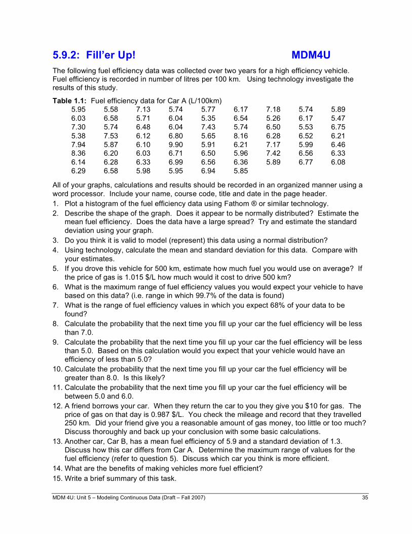
5.9.2: Fill’er Up! MDM4U

The following fuel efficiency data was collected over two years for a high efficiency vehicle. Fuel efficiency is recorded in number of litres per 100 km. Using technology investigate the results of this study.

Table 1.1: Fuel efficiency data for Car A (L/100km) 5.95 5.58 7.13 5.74 5.77 6.17 7.18 5.74 5.89 6.03 6.58 5.71 6.04 5.35 6.54 5.26 6.17 5.47 7.30 5.74 6.48 6.04 7.43 5.74 6.50 5.53 6.75 5.38 7.53 6.12 6.80 5.65 8.16 6.28 6.52 6.21 7.94 5.87 6.10 9.90 5.91 6.21 7.17 5.99 6.46 8.36 6.20 6.03 6.71 6.50 5.96 7.42 6.56 6.33 6.14 6.28 6.33 6.99 6.56 6.36 5.89 6.77 6.08 6.29 6.58 5.98 5.95 6.94 5.85

All of your graphs, calculations and results should be recorded in an organized manner using a word processor. Include your name, course code, title and date in the page header. 1. Plot a histogram of the fuel efficiency data using Fathom ® or similar technology. 2. Describe the shape of the graph. Does it appear to be normally distributed? Estimate the

mean fuel efficiency. Does the data have a large spread? Try and estimate the standard deviation using your graph.

3. Do you think it is valid to model (represent) this data using a normal distribution? 4. Using technology, calculate the mean and standard deviation for this data. Compare with

your estimates. 5. If you drove this vehicle for 500 km, estimate how much fuel you would use on average? If

the price of gas is 1.015 $/L how much would it cost to drive 500 km? 6. What is the maximum range of fuel efficiency values you would expect your vehicle to have

based on this data? (i.e. range in which 99.7% of the data is found) 7. What is the range of fuel efficiency values in which you expect 68% of your data to be

found? 8. Calculate the probability that the next time you fill up your car the fuel efficiency will be less

than 7.0. 9. Calculate the probability that the next time you fill up your car the fuel efficiency will be less

than 5.0. Based on this calculation would you expect that your vehicle would have an efficiency of less than 5.0?

10. Calculate the probability that the next time you fill up your car the fuel efficiency will be greater than 8.0. Is this likely?

11. Calculate the probability that the next time you fill up your car the fuel efficiency will be between 5.0 and 6.0.

12. A friend borrows your car. When they return the car to you they give you $10 for gas. The price of gas on that day is 0.987 $/L. You check the mileage and record that they travelled 250 km. Did your friend give you a reasonable amount of gas money, too little or too much? Discuss thoroughly and back up your conclusion with some basic calculations.

13. Another car, Car B, has a mean fuel efficiency of 5.9 and a standard deviation of 1.3. Discuss how this car differs from Car A. Determine the maximum range of values for the fuel efficiency (refer to question 5). Discuss which car you think is more efficient.

14. What are the benefits of making vehicles more fuel efficient? 15. Write a brief summary of this task.


5.9.3: Sample “Fill’er Up!” Rubric MDM4U Questions: Level 1 Level 2 Level 3 Level 4 1. Graph Does not use graphing

software effectively, or more than 2 items are missing

Uses graphing software effectively; two items missing

Uses graphing software effectively; one item missing

Uses graphing software effectively; Axes are correctly labelled; title is clear and descriptive; bin sizes are appropriate

2. Estimations Estimates are completely incorrect; no logical mathematical thought is evident

Estimates are okay and demonstrate logical mathematical thought.

Estimates are well done and demonstrate logical mathematical thought

Estimates are excellent and clearly demonstrate thought and mathematical intuition.

3. Validity No discussion of validity is given.

Basic discussion of validity is presented.

Thorough discussion of validity is given.

Thorough discussion of validity is given. Student outlines multiple reasons for validity and states limitations of the model.

4. Mean and StdDev.

Calculation of mean and standard deviation are incorrect.

Calculation of mean and standard deviation are correct; however the mathematical notation is incorrect or reported incorrectly.

Calculation of mean and standard deviation are correct; mathematical notation is okay. Most steps shown using equation editor.

Calculation of mean and standard deviation are correct and reported using proper mathematical notation. All steps shown using equation editor.

5. Cost Calculation

Calculation of cost is incorrect.

Calculation of cost is correct; however the mathematical notation is incorrect or reported incorrectly.

Calculation of cost is correct; mathematical notation is okay. Most steps shown using equation editor.

Calculation of cost is correct and reported using proper mathematical notation. . All steps shown using equation editor.

6. Maximum range

Range is incorrect. Student reports the correct maximum range; however the mathematical notation is incorrect or reported incorrectly.

Student reports the correct maximum range; mathematical notation is okay. Most steps shown using equation editor.

Student reports the correct maximum range using proper mathematical notation. All steps shown using equation editor.

7. Mid range Range is incorrect. Student reports the correct mid range; however the mathematical notation is incorrect or reported incorrectly.

Student reports the correct mid range; mathematical notation is okay. Most steps shown using equation editor.

Student reports the correct mid range using proper mathematical notation. All steps shown using equation editor.

8. Probability calc.

Probability calculation is incorrect.

Probability calculation is correct; however the mathematical notation is incorrect or reported incorrectly.

Probability calculation is correct; mathematical notation is okay. Most steps shown using equation editor.

Probability calculation is correct and reported using proper mathematical notation. All steps shown using equation editor.
















12. Borrowing Q. Student does not answer the question correctly and does not back up any of their work with calculations.

Student answers the question with some degree of correctness, but does not back up their answer with calculations.

Calculations are correct and complete. Student uses one calculation to accurately back up their answers. Mathematical notation is correct.

Calculations are correct and complete. Student uses multiple calculations to accurately back up their answers. Mathematical notation is correct. Answers show insight.

13. Car B Q. Calculations are incorrect; proper mathematical notion is not used; discussion is incomplete and not related to the calculations.

Calculations are correct and proper mathematical notion is used. All steps shown using equation editor. Discussion is incomplete or not related to calculations.

Calculations are correct and proper mathematical notion is used. All steps shown using equation editor. Discussion is okay.

Calculations are correct and proper mathematical notion is used. All steps shown using equation editor. Discussion is insightful and refers to calculations.

14. Benefits No discussion is given. One reason is given for why it is beneficial to make more efficient use of cars.

Some reasons are given for why it is beneficial to make more efficient use of cars.

Multiple, insightful reasons are given for why it is beneficial to make more efficient use of cars.

15. Summary Summary is incomplete. Summary is okay, but some major points are missing.

Summary is complete, well organized, but not concise.

Summary is concise and complete. Summary refers to specific techniques used and reasons for modelling data using normal distributions.

Communication: Level 1 Level 2 Level 3 Level 4 Report format Report is not type written,

equation editor is not used, headers are missing, titles are missing

Report is well communicated and type written. Two or more formatting items are missing.

Report is well communicated and type written. One formatting item is missing.

Report is clearly presented and type written. Equation editor is used. Headers and page numbers are included. Main title and sub section titles are included and descriptive.

Documents

Unit 5 : Day 1 : Continuous Data MDM4U Description ...edugains.ca/resources/LearningMaterials/TIPS/tips4rm/mdm4u/Unit5... · MDM 4U: Unit 5 – Modeling Continuous Data (Draft –