Unit 2: Review of Probability - University of Tennesseeweb.utk.edu/~leon/stat571/2004SummerPDFs/571Unit2.pdf · 6/7/2007 Unit 2 - Stat 571 - Ramón V. León 1 Unit 2: Review of Probability

6/7/2007 Unit 2 - Stat 571 - Ramón V. León 1

Unit 2: Review of Probability

Statistics 571: Statistical MethodsRamón V. León


Approaches to Probability• Approaches to probability

– Classical approach– Frequentist– Personal or subjective approach– Axiomatic approach

• Basic ideas of axiomatic approach– Sample space– Events– Union– Intersection– Complement– Disjoint or mutually exclusive events– Inclusion


Axioms of Probability• Axioms:

– P(A) ≥0– P(S) = 1 where S is the sample space– P(A ∪ B) = P(A) + P(B) if A and B are mutually

exclusive events• Theorems about probability can be proved using these

axioms• These theorems can be used in probability calculations

– E.g. assuming all elements of the sample space are equally likely

– Counting arguments used. (Take a look at Birthday Problem on Page 13.)


Conditional Probability and Independence• Conditional probability

– P(A | B) = P (A ∩ B) / P(B)• Events A and B are mutually independent if P (A | B) = P(A)

– Implies P (A ∩ B) = P(A)P(B)


Tossing Two Dice

(6,6)(6,5)(6,4)(6,3)(6,2)(6,1)6(5,6)(5,5)(5,4)(5,3)(5,2)(5,1)5(4,6)(4,5)(4,4)(4,3)(4,2)(4,1)4(3,6)(3,5)(3,4)(3,3)(3,2)(3,1)3

(2,6)(2,5)(2,4)(2,3)(2,2)(2,1)2(1,6)(1,5)(1,4)(1,3)(1,2)(1,1)1

654321

First Die Outcome

Second Die Outcome

Sample space has 6 x 6 = 36 outcomes


Conditional Probability Example

P(A)=8/36

P(B)=18/36


AIDS Example

100009900100

941094055TestNegative

59049595Test positive

Not AIDSAIDS

P(A) = 100/10000 =.01 P(+|A) = 95/100 =.95 P(-|~A) = 9405/9900 =.95P(A|+) = 95/590 =.16

The usual way of solving this problem uses Bayes Theorem

Given

Conclude


What Does a Positive HIV Test Means?


Bayes Theorem Consequences

( ) ( | )P A P A B⎯⎯→

( | ) ( | )P A B P B A≠

( ) ( | )P A P A Data⎯⎯→


Independence Example


Random Variables

• A random variable (r.v.) associates a unique numerical value with each outcome in the sample space

• Example:

• Discrete random variables: number of possible values is finite or countably infinite: x1, x2, x3, x4, x5, x6, …

• Probability mass (density) function (p.m.f. or p.d.f.)– f(x) = P(X= x )

• Cumulative distribution function (c.d.f.)

– F(x) = P (X ≤ x) =

10

X ⎧= ⎨

⎩

if coin toss results in a head

if coin toss results in a tail

( )k x

f k≤∑


Discrete Random Variable Example


Graphs of Probability Mass (Density) Function and Probability Distribution Function


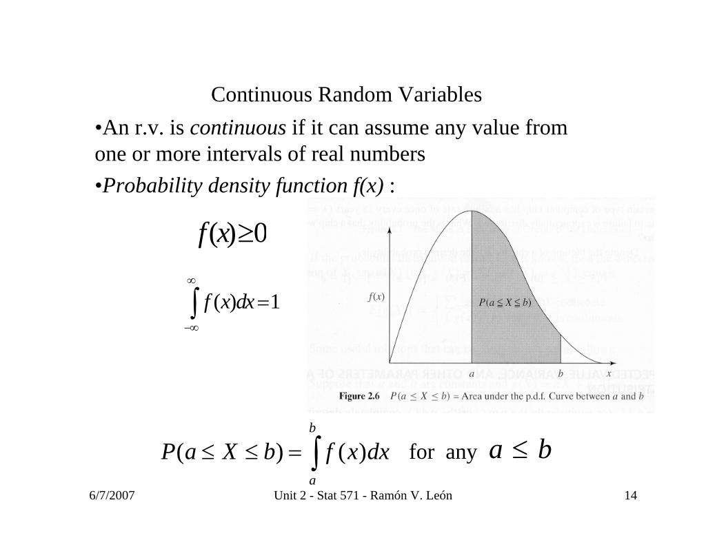
Continuous Random Variables

( ) 0f x ≥

•An r.v. is continuous if it can assume any value from one or more intervals of real numbers•Probability density function f(x) :

( ) 1f x dx∞

−∞

=∫

( ) ( )b

a

P a X b f x dx≤ ≤ = ∫ for any a b≤


Cumulative Distribution Function

The cumulative distribution function (c.d.f.), denoted by F(x) , for a continuous random variable is given by:

( ) ( ) ( )x

F x P X x f y dy−∞

= ≤ = ∫

It follows that ( )( ) dF xf x

dx=

x

f(x)F(x)


Exponential Distribution Example


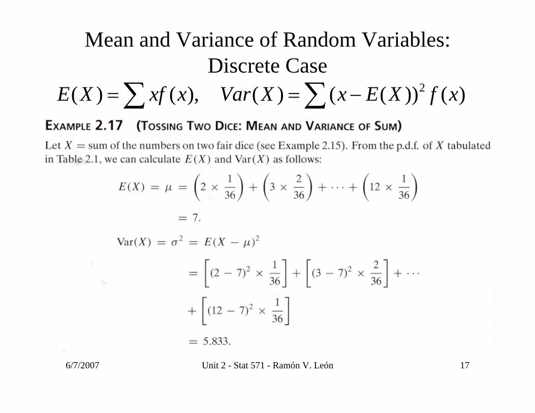
Mean and Variance of Random Variables: Discrete Case

2( ) ( ), ( ) ( ( )) ( )E X xf x Var X x E X f x= = −∑ ∑


Mean and Variance of Sum of Two Dice Tosses


Expected Value or Mean of Random Variables

The expected value or mean of a discrete r. v. X denoted by E(X), μX , or simply μ, is defined as:

1 1 2 2( ) ( ) ( ) ( ) ...x

E X xf x x f x x f xμ= = = + +∑The expected value of a continuous r. v. is defined as:

( ) ( )E X xf x dxμ= = ∫

0

Mean of Exponetial Distribution 1( ) xE X x e dxλλλ

∞ −= =∫


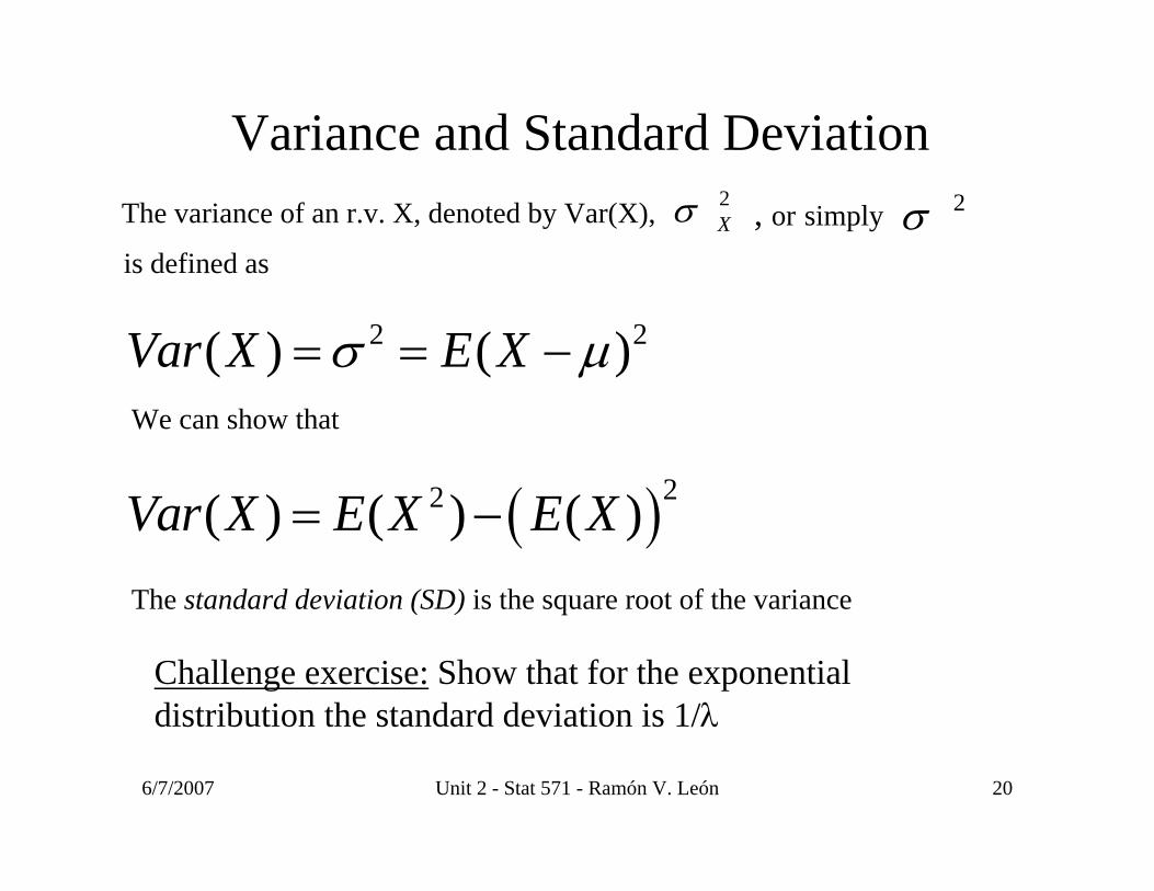
Variance and Standard DeviationThe variance of an r.v. X, denoted by Var(X), 2

Xσ , or simply 2σis defined as

2 2( ) ( )Var X E Xσ μ= = −We can show that

( )22( ) ( ) ( )Var X E X E X= −The standard deviation (SD) is the square root of the variance

Challenge exercise: Show that for the exponential distribution the standard deviation is 1/λ


Variance of the Mean of independent, Identically Distributed Random Variables

( )( )

1

2 1

2 1

22

2

( )

1

1

1

nii

nii

nii

XVar X Var

n

Var Xn

Var Xn

nn

n

σ

σ

=

=

=

⎛ ⎞⎜ ⎟=⎜ ⎟⎝ ⎠

⎛ ⎞= ⎜ ⎟⎝ ⎠⎛ ⎞= ⎜ ⎟⎝ ⎠⎛ ⎞= ⎜ ⎟⎝ ⎠

=

∑

∑

∑ by independence

since the r.v.’s are identically distributed

1 2

We often refer to , ,..., as

a randon samplewith replacement orfrom a very large population

nX X X


Quantiles and PercentilesFor 0 1p≤ ≤ the pth quantile (or the 100pth percentile), denoted by

pθ ,of a continuous r.v. X is defined by the following equation:

( ) ( )p pP X F pθ θ≤ = =

.5θ is called the median

pF(x)

θp


Exponential Distribution Percentiles


Jointly Distributed Random Variables

( , ) joint probability mass function

f x y =

32 0.16200

=


Marginal Distribution

Discrete: ( ) ( ) ( , )

Continuous: ( ) ( ) ( , )

y

X

g x P X x f x y

g x f x f x y dy∞

−∞

= = =

= =

∑

∫


Conditional Distribution

( , )( | ) ( | )( )

f x yf y x P Y y X xg x

= = = =

Conditional probability mass function (p.m.f.):( 4, 1) 0.005( 1| 4)

( 4) 0.315P X YP Y X

P X= =

= = = ==


Independent Random Variables and are independent r.v.'s if ( , ) ( ) ( )

( , )Note that ( | ) ( )( )

X Y f x y g x h yf x yf y x h yg x

=

= =


Covariance and Correlation

If X and Y are independent then E(XY)=E(X)E(Y) so the covarianceis zero. The other direction is not true; zero covariance does not imply independence.

( , ) ( )( ) ( ) ( ) ( )XY X YCov X Y E X Y E XY E X E Yσ μ μ= = − − = −

Note that: ( ) ( , )E XY xyf x y dxdy∞ ∞

−∞ −∞= ∫ ∫

( , )( , )var( ) var( )

XYXY

X Y

Cov X Ycorr X YX Y

σρσ σ

= = =

Measures strength of linear association

1 1XYρ− ≤ ≤


Covariance Example

•A positive covariance indicates positive dependence•A negative covariance indicates negative dependence


Correlation Example


Chebyshev’s InequalityLet c > 0 be a constant. Then irrespective of thedistribution of X

2

( )( ( ) ) Var XP X E X cc

− ≥ ≤


Weak Law of Large Numbers

Let X be the sample mean of n i.i.d. observations from a

population with finite mean μ and variance 2σ . Then forany fixed c > 0

2

2( ) 0P X cncσμ− ≥ ≤ → as n→∞

We see that X approaches μ as n gets large.

This follows from Chebyshev’s inequality and the fact that2

( ) and ( )E X Var Xnσμ= =


Selected Discrete Distributions

Bernoulli distribution:

( ) ( )1p

f x P X xp

⎧= = = ⎨ −⎩

if x = 1if x = 0

( ) ,E X p= ( ) (1 )V ar X p p= −

Binomial distribution:

( ) ( ) (1 )x n xnf x P X x p p

x−⎛ ⎞

= = = −⎜ ⎟⎝ ⎠

for x = 0, 1, …,n

( ) ,E X np= ( ) (1 )Var X np p= −

( )5! 5!, e.g., 103! ! 3!2!

n nk k n k⎛ ⎞ ⎛ ⎞

= = =⎜ ⎟ ⎜ ⎟−⎝ ⎠ ⎝ ⎠


Binomial Distribution Example

Suppose that the probability of a thumbtack landing with the pin up is 0.9. If we toss the thumbtack ten times what is the probability that it lands with the pin up exactly 7 times?

7 3 7 310( 7) (.9) (1 .9) 120(.9) (.1) .057

7P X ⎛ ⎞

= = − = =⎜ ⎟⎝ ⎠

Answer:

See Example 2.30, Page 43 for another application of the Binomial distribution

( ) 10 .9 9, ( ) (1 ) 10 .9 .1 .9E X np Var X np p= = × = = − = × × =

Also note:


Hypergeometric Distribution(Sampling without replacement from a small population)

A lot of 50 tables has two defective tables. A sample of five tables are selected without replacement. What is the probabilitythat none of these five tables is defective?

2 480 5

( 0) .8082505

P X

⎛ ⎞⎛ ⎞⎜ ⎟⎜ ⎟⎝ ⎠⎝ ⎠= = =⎛ ⎞⎜ ⎟⎝ ⎠

Suppose the five tables had been selected with replacement? What would then be the probability?

0 55 2 48( 0) .81540 50 50

P X ⎛ ⎞⎛ ⎞ ⎛ ⎞= = =⎜ ⎟⎜ ⎟ ⎜ ⎟⎝ ⎠ ⎝ ⎠⎝ ⎠


( ) ( ) ,!

xef x P X xx

λλ−

= = = for x = 0, 1, 2, …

( ) ,E X λ= ( )Var X λ=

Poisson Distribution:

Example: On the average five Prussian soldiers die from horsekicks in a year. What is the probability that exactly four soldiers are killed this way in a given year?

5 4(5)( 4) .1754!

eP X−

= = =


Geometric Distribution

Probability of waiting time to an event in independent trials

1

2

( ) (1 ) , 1, 2,...1 1( ) and ( )

xP X x p p xpE X Var X

p p

−= = − =−

= =

Suppose the probability of winning the jackpot in a slot machineis .01. What is the expected number of tries to win the jackpot?What the is the probability that you hit the jackpot for the first time on your fifth try?

41( ) 100, ( 5) (.99) (.01) .0096.01

E X P X= = = = =


Uniform DistributionDistribution when all values in an interval are equally likely

Suppose that you select a real number at random in the interval [1,5]. What is the probability that it turns out to be between 2and 4?

4 2(2 4) 0.55 1

P X −≤ ≤ = =

−Proportion of the lengths of the intervals [2,4] to the length of the interval [1,5]


Exponential DistributionDistribution of waiting time when arrivals occur at random

0( ) , ( ) 1 for 0

xx t xf x e F x e dt e xλ λ λλ λ− − −= = = − ≥∫2

1 1( ) and ( )E X Var Xλ λ

= =

( ) 1 ( ) 1 ( ) xP X x P X x F x e λ−> = − ≤ = − =


Memoryless Property of the Exponential Distribution

( ) ( )( ) ( )

|

5 3 | 5 3

P X s t X s P X t

P X X P X

> + > = >

> + > = >

The probability of having to wait t additional minutes after havingwaited s minutes is the same as the probability of having to wait t minutes to begin with.


Normal DistributionA continuous r.v. X has a normal distribution with parameter μand 2σ if its p.d.f. is given by

2

2( )

21( ) for 2

x

f x e xμσ

σ π

−−

= −∞< <∞

( )E X μ= 2( )Var X σ=and

2~ ( , )X N μ σNotation:


Standard Normal Distribution = N(0,1)2If ~ ( , ) then ~ (0,1)XX N Z Nμμ σ

σ−

=

( ) X x xP X x P Z μ μ μσ σ σ− − −⎛ ⎞ ⎛ ⎞≤ = = ≤ = Φ⎜ ⎟ ⎜ ⎟

⎝ ⎠ ⎝ ⎠

2~ (205,5 )( 200)

205 200 2055 5

( 1) ( 1) 0.1587

X NP X

XP Z

P Z

< =

− −⎛ ⎞= < =⎜ ⎟⎝ ⎠

< − = Φ − =


Standard Normal Table


Empirical Rule


Mean of i.i.d. Normal Random Variable

1 2

21 2

2

21

Let , ,..., be independent, indentically

distributed ( , ). We say that , ,...,

is a random sample from a ( , ) population.

Then for we have ~ , .

n

n

nii

X X X

N X X X

N

XX X N

n n

μ σ

μ σ

σμ= ⎛ ⎞= ⎜ ⎟

⎝ ⎠

∑

Hint: Use this result to do homework problem 2.83


Percentiles of the Normal Distribution

Suppose that the scores on a standardized test are normally distributed with mean 500 and standard deviation 100. Whatis the 75th percentile score of this test?

500 500 500 500( ) .75100 100 100 100

X x x xP X x P P Z− − − −⎛ ⎞ ⎛ ⎞ ⎛ ⎞≤ = ≤ = ≤ = Φ =⎜ ⎟ ⎜ ⎟ ⎜ ⎟⎝ ⎠ ⎝ ⎠ ⎝ ⎠

500 0.675 500 (0.675)(100) 567.5100

x x−= ⇒ = + =

From Table A.3 (0.675) 0.75.Φ = So

For 75 percentile means that ( ) .75. Sothx P X x= ≤ =

Documents

Unit 2: Review of Probability - University of Tennesseeweb.utk.edu/~leon/stat571/2004SummerPDFs/571Unit2.pdf · 6/7/2007 Unit 2 - Stat 571 - Ramón V. León 1 Unit 2: Review of Probability