UNIT - 1 INTRODUCTION TO DATA STRUCTURES, SEARCHING … · Simple and Compound Data Structures •Simple Data Structure: Simple data structure can be constructed with the help of

UNIT - 1

INTRODUCTION TO DATA

STRUCTURES, SEARCHING

AND SORTING

B.Padmaja

Associate Professor

Department of CSE

Institute of Aeronauitcal Engineering

2

Contents

• Introduction to Data Structures

• Classification and Operations on Data Structures

• Preliminaries of Algorithm

• Algorithm Analysis and Complexity

• Recursive Algorithms

• Searching Techniques - Linear, Binary, Fibonacci

• Sorting Techniques- Bubble, Selection, Insertion,

Quick and Merge Sort

• Comparison of Sorting Algorithms

3

Introduction to Data Structures

• A data structure is a way of storing data in a

computer so that it can be used efficiently and

it will allow the most efficient algorithm to be

used.

• A data structure should be seen as a logical

concept that must address two fundamental

concerns.

I. First, how the data will be stored, and

II. Second, what operations will be performed on it.

Classification of Data Structures

• Data structures can be classified as i. Simple data structure

ii. Compound data structure

iii. Linear data structure

iv. Non linear data structure

Fig. Classification of Data Structures 4

Simple and Compound Data Structures

• Simple Data Structure: Simple data structure can be

constructed with the help of primitive data structure.

A primitive data structure used to represent the

standard data types of any one of the computer

languages. Variables, arrays, pointers, structures,

unions, etc. are examples of primitive data structures.

Compound Data structure: Compound data

structure can be constructed with the help of any one

of the primitive data structure and it is having a

specific functionality. It can be designed by user. It

can be classified as

i. Linear data structure

ii. Non-linear data structure 5

6

Linear and Non-linear Data Structures

• Linear Data Structure: Linear data structures can be

constructed as a continuous arrangement of data

elements in the memory. It can be constructed by

using array data type. In the linear Data Structures the

relationship of adjacency is maintained between the

data elements.

• Non-linear

structure can

Data Structure: Non-linear data

be constructed as a collection of

randomly distributed set of data item joined together

by using a special pointer (tag). In non-linear Data

structure the relationship of adjacency is not

maintained between the data items.

7

Operations on Data Structures

i. Add an element

ii. Delete an element

iii. Traverse

iv. Sort the list of elements

v. Search for a data element

8

Abstract Data Type

• An abstract data type, sometimes abbreviated

ADT, is a logical description of how we view

the data and the operations that are allowed

without regard to how they will be

implemented.

• By providing this level of abstraction, we are

creating an encapsulation around the data. The

idea is that by encapsulating the details of the

implementation, we are hiding them from the

user‘s view. This is called information hiding.

9

Algorithm Definition

• An Algorithm may be defined as a finite

sequence of instructions each of which has a clear

meaning and can be performed with a finite

amount of effort in a finite length of time.

• The word algorithm originates from the Arabic

word Algorism which is linked to the name of the

Arabic Mathematician AI Khwarizmi.

• AI Khwarizmi is considered to be the first

algorithm designer for adding numbers.

10

Structure of an Algorithm

• An algorithm has the following structure:

– Input Step

–Assignment Step

–Decision Step

–Repetitive Step

–Output Step

11

Properties of an Algorithm

• Finiteness:- An algorithm must terminate after

finite number of steps.

• Definiteness:-The steps of the algorithm must be

precisely defined.

• Generality:- An algorithm must be generic

enough to solve all problems of a particular

class.

• Effectiveness:- The operations of the algorithm

must be basic enough to be put down on pencil

and paper.

Input-Output:- The algorithm must have certain

initial and precise inputs, and outputs that may be

generated both at its intermediate and final steps

13

Algorithm Analysis and Complexity

• The performances of algorithms can be

measured on the scales of Time and Space.

• The Time Complexity of an algorithm or a

program is a function of the running time of

the algorithm or a program.

• The Space Complexity of an algorithm or a

program is a function of the space needed by

the algorithm or program to run to completion.

14


• The Time Complexity of an algorithm can be computed either by an – Empirical or Posteriori Testing

– Theoretical or Apriori Approach

• The Empirical or Posteriori Testing approach calls for implementing the complete algorithm and executes them on a computer for various instances of the problem.

• The Theoretical or Apriori Approach calls for mathematically determining the resources such as time and space needed by the algorithm, as a function of parameter related to the instances of the problem considered.

15


• Apriori analysis computed the efficiency of the

program as a function of the total frequency

count of the statements comprising the

program.

• Example: Let us estimate the frequency count

of the statement x = x+2 occurring in the

following three program segments A, B and C.

16

Total Frequency Count of Program

Segment A

• Program Statements

..…………………

x = x+ 2

….……………….

Total Frequency Count

• Frequency Count

1

1

Time Complexity of Program Segment A is O(1).

17


Segment B

• Program Statements

..…………………

for k = 1 to n do

x = x+ 2;

end

….……………….


• Frequency Count

(n+1)

n

n

……………………

3n+1

Time Complexity of Program Segment B is O(n).

18


Segment C • Program Statements

..…………………

for j = 1 to n do for k = 1 to n do

x = x+ 2;

end

end

….……………….


• Frequency Count

(n+1) (n+1)n n2

n2

n …………………………

3n2 +3n+1

Time Complexity of Program Segment C is O(n2).

19

Asymptotic Notations

• Big oh(O): f(n) = O(g(n)) ( read as f of n is big

oh of g of n), if there exists a positive integer

n0 and a positive number c such that |f(n)| ≤ c

|g(n)| for all n ≥ n0.

• Here g(n) is the upper bound of the function

f(n).

f(n) g(n)

16n3 + 45n2 + 12n n3 f(n) = O(n3 )

34n – 40 n f(n) = O(n)

50 1 f(n) = O(1)

20


• Omega(Ω): f(n) = Ω(g(n)) ( read as f of n is

omega of g of n), if there exists a positive

integer n0 and a positive number c such that

|f(n)| ≥ c |g(n)| for all n ≥ n0.

• Here g(n) is the lower bound of the function

f(n).

f(n) g(n)

16n3 + 8n2 + 2 n3 f(n) = Ω (n3 )

24n +9 n f(n) = Ω (n)


• Theta(Θ): f(n) = Θ(g(n)) (read as f of n is

theta of g of n), if there exists a positive

integer n0 and two positive constants c1 and c2

such that c1 |g(n)| ≤ |f(n)| ≤ c2 |g(n)| for all n ≥

n0.

• The function g(n) is both an upper bound and a

lower bound for the function f(n) for all values

of n, n ≥ n0 20

f(n) g(n)

16n3 + 30n2 – 90 n2 f(n) = Θ(n2 )

7. 2n + 30n 2n f(n) = Θ (2n)

22


• Little oh(o): f(n) = O(g(n)) ( read as f of n is

little oh of g of n), if f(n) = O(g(n)) and f(n) ≠

Ω(g(n)).

f(n) g(n)

18n + 9 n2 f(n) = o(n2) since f(n) = O(n2 ) and f(n) ≠ Ω(n2 ) however f(n) ≠ O(n).

23

Time Complexity

Complexity Notation Description

Constant O(1) Constant number of operations, not depending on the

input data size.

Logarithmic O(logn) Number of operations proportional of log(n) where n

is the size of the input data.

Linear O(n) Number of operations proportional to the input data

size.

Quadratic O(n2 ) Number of operations proportional to the square of

the size of the input data.

Cubic O(n3 ) Number of operations proportional to the cube of the

size of the input data.

Exponential O(2n) Exponential number of operations, fast growing.

O(kn )

O(n!)

Time Complexities of various

Algorithms

24

25

Recursion Examples

Factorial Function

Factorial(Fact, N)

1. If N = 0, then set Fact :=1, and return.

2. Call Factorial(Fact, N-1)

3. Set Fact := N* Fact

4. Return

26

Fibonacci Sequence

Fibonacci(Fib, N)

1. If N=0 or N=1, then: Set Fib:=N, and return.

2. Call Fibonacci(FibA, N-2)

3. Call Fibonacci(FibB, N-1)

4. Set Fib:=FibA + FibB

5. Return

27

Towers of Hanoi

Tower(N, Beg, Aux, End)

1. If N=1, then:

(a) Write: Beg -> End

(b) Return

2. [Move N-1 disks from peg Beg to peg Aux]

Call Tower(N-1, Beg, End, Aux)

3. Write: Beg -> End

4. [Move N-1 disks from peg Aux to peg End]

Call Tower(N-1, Aux, Beg, End)

5. Return

28

Basic Searching Methods

• Search: A search algorithm is a method of

locating a specific item of information in a

larger collection of data.

• There are three primary algorithms used for

searching the contents of an array:

1. Linear or Sequential Search

2. Binary Search

3. Fibonacci Search

29

Linear Search

• Begins search at first item in list, continues

searching sequentially(item by item) through

list, until desired item(key) is found, or until

end of list is reached.

• Also called sequential or serial search.

• Obviously not an

searching ordered

efficient method for

lists like phone

directory(which is ordered alphabetically).

30

Linear Search contd..

• Advantages

1. Algorithm is simple.

2. List need not be ordered in any particular

way.

• Time Complexity of Linear Search is O(n).

31

Recursive Linear Search Algorithm

def linear_Search(l,key,index=0):

if l:

if l[0]==key:

return index

s=linear_Search(l[1:],key,(index+1))

if s is not false:

return s

return false

32

Binary Search

• List must be in sorted order to begin with

Compare key with middle entry of list

For lists with even number of entries, either

of the two middle entries can be used.

• Three possibilities for result of comparison

Key matches middle entry --- terminate

search with success

Key is greater than middle entry ---

matching entry(if exists) must be in upper

part of list (lower part of list can be

discarded from search)

33

Binary Search contd…

Key is less than middle entry ---matching

entry (if exists) must be in lower part of list (

upper part of list can be discarded from

search)

• Keep applying above 2 steps to the

progressively ―reduced‖ lists, until match is

found or until no further list reduction can be

done.

• Time Complexity of Binary Search is O(logn).

34

Fibonacci Search

• Fibonacci Search Technique is a method of

searching a sorted array using a divide and

conquer algorithm that narrows down possible

locations with the aid of Fibonacci numbers.

• Fibonacci search examines locations whose

addresses have lower dispersion, therefore it

has an advantage over binary search in slightly

reducing the average time needed to access a

storage location.

35

Fibonacci Search contd…

search has a complexity of • Fibonacci

O(log(n)).

• Fibonacci search was first devised by

Kiefer(1953) as a minimax search for the

maximum (minimum) of a unimodal function

in an interval.

36

Fibonacci Search Algorithm

• Let k be defined as an element in F, the array

of Fibonacci numbers. n = Fm is the array size.

If the array size is not a Fibonacci number, let

Fm be the smallest number in F that is greater

than n.

• The array of Fibonacci numbers is defined

where Fk+2

= Fk+1 + Fk, when k ≥ 0, F1 = 1, and F0 = 0.

• To test whether an item is in the list of ordered

numbers, follow these steps:

Set k = m.

If k = 0, stop. There is no match; the item is

not in the array.

38

Fibonacci Search Algorithm Contd…

• Compare the item against element in Fk−1.

• If the item matches, stop.

• If the item is less than entry Fk−1, discard

the elements from positions Fk−1 + 1 to n.

Set k = k − 1 and return to step 2.

• If the item is greater than entry Fk−1,

discard the elements from positions 1 to

Fk−1. Renumber the remaining elements

from 1 to Fk−2, set k = k − 2, and return to

step 2.

39

Basic Sorting Methods :-Bubble Sort • First Level Considerations

• To sort list of n elements in ascending order

Pass 1 :make nth element the largest

Pass 2 :if needed make n-1th element the 2nd

largest

Pass 3 :if needed make n-2th element the 3rd

largest Pass n-2: if needed make 3rd n-(n-3)th element the (n-2)th largest Pass n-1 :if needed make 2nd n-(n-2)th element the (n-1)th largest

• Maximum number of passes is (n-1).

40

Bubble Sort

Second Level Considerations

• Pass 1: Make nth element the largest.

Compare each successive pair of elements

beginning with 1st 2nd and ending with n-1th

nth and swap the elements if necessary.

• Pass 2 : Make n-1th element the 2nd largest.


beginning with 1st 2nd and ending with n-2th

n-1th and swap the elements if necessary

Pass n-1:Make 2nd n-(n-2)th element the (n-1)th

largest.


beginning with 1st 2nd and ending with n-(n-1)

th n-(n-2)th 1st 2nd and swap the elements if

necessary.

List is sorted when either of the following occurs

No swapping involved in any pass

Pass n-1:the last pass has been executed

Bubble Sort Example

42

43

Selection Sort

First Level Considerations

• To sort list of n elements in ascending order

• Pass 1: make 1st element the smallest

• Pass 2: make 2nd element the 2nd smallest

• Pass 3: make 3rd element the 3rd smallest

• Pass n-2: make (n-2)th element the (n-2)th smallest

• Pass n-1: make (n-1)th element the (n-1)th smallest

• Number of passes is (n-1).

44

Selection Sort

Second Level Considerations • Pass 1: Make 1st element the smallest

Examine list from 1st to last element locate element with smallest value and swap it with the 1st element where appropriate .

• Pass 2: Make 2nd element the 2nd smallest Examine list from 2nd to last element locate element with smallest value and swap it with the 2nd element where appropriate.

• Pass n-1: Make (n-1)th element the (n-1)th smallest Examine list from (n-1)th to last element locate element with smallest value and swap it with the n-1th element where appropriate.

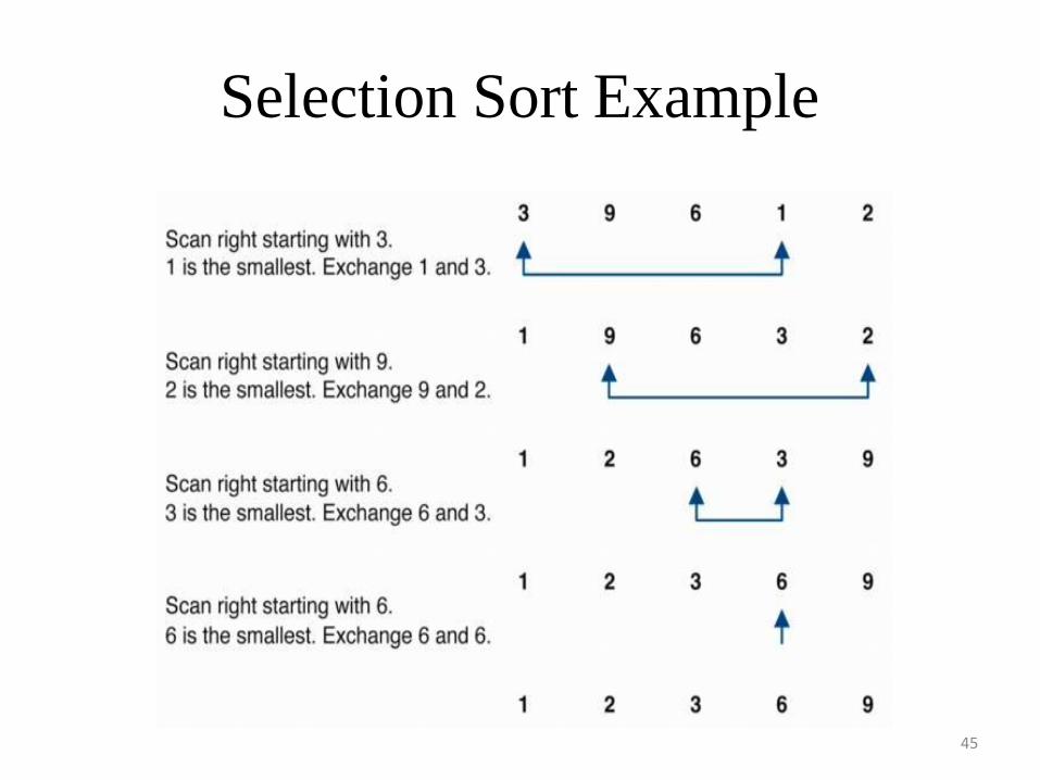
Selection Sort Example

45

46

Insertion Sort

First Level Considerations

To sort list of n items (stored as 1D array) in ascending order

• NOTE: 1-element sub-array (1st) is always sorted

• Pass 1: make 2-element sub-array (1st 2nd) sorted

• Pass 2 :make 3-element sub-array (1st 2nd 3rd) sorted

• Pass 3 :make 4-element sub-array (1st 4th) sorted

• Pass n-2: make n-1-element sub-array (1st (n-1)th) sorted

• Pass n-1: make entire n-element array (1st nth) sorted

• Number of passes is (n-1)

Insertion Sort Example

47

48

Quick Sort

It uses Divide-and-Conquer approach:

1. Divide: partition A[p..r] into two sub-arrays A[p..q-1] and A[q+1..r] such that each element of A[p..q-1] is ≤ A[q], and each element of A[q+1..r] is ≥ A[q]. Compute q as part of this partitioning.

2. Conquer: sort the sub-arrays A[p..q-1] and

A[q+1..r] by recursive calls to QUICKSORT.

3. Combine: the partitioning and recursive sorting leave us with a sorted A[p..r] – no work needed here.

The Pseudo-Code of Quick Sort

49

Quick Sort Contd…..

50

51

Quick sort Analysis

• Best case running time: O(n log2n)

• Worst case running time: O(n2)!!!

Quick Sort Example

52

53

Merge Sort • Merge-sort is a sorting algorithm based on the divide-and-

conquer paradigm

• Like heap-sort

It uses a comparator

It has O(n log n) running time

• Unlike heap-sort

It does not use an auxiliary priority queue

It accesses data in a sequential manner (suitable to sort data

on a disk)

• Merge-sort on an input sequence S with n elements consists of three steps: Divide: partition S into two sequences S1 and S2 of about n/2 elements each

Recur: recursively sort S1 and S2

Conquer: merge S1 and S2 into a unique sorted sequence

54

Merge Sort Algorithm

Algorithm mergeSort(S, C)

Input sequence S with n elements, comparator C

Output sequence S sorted according to C

if S.size() > 1

(S1, S2) partition(S, n/2)

mergeSort(S1, C)

mergeSort(S2, C)

S merge(S1, S2)

Merge Sort Example

55

Merge Sort Example Contd…

56

57

Analysis of Merge Sort

• The height h of the merge-sort tree is O(log n)

– at each recursive call we divide in half the sequence,

• The overall amount or work done at the nodes of depth

i is O(n)

– we partition and merge 2i sequences of size n/2i

– we make 2i+1 recursive calls

• Thus, the total running time of merge-sort is O(n log n)

Comparison of Sorting Algorithms

58

UNIT - 2

LINEAR DATA STRUCTURES

B.Padmaja

Associate Professor

Department of CSE


Contents

• Stack - Primitive Operations and Implementation

• Applications of Stack

• Queue - Primitive Operations and Implementation

• Linear Queue operations

• Applications of Linear Queue

• Circular Queue operations

• Priority Queue

• Double Ended Queue (Deque)

Stacks

• A stack is a list of elements in which an

element may be inserted or deleted only at one

end, called the top of the stack.

• The elements are removed from a stack in the

reverse order of that in which they were

inserted into the stack.

• Stack is also known as a LIFO (Last in Fast

out) list or Push down list.

Basic Stack Operations

PUSH: It is the term used to insert an element

into a stack.

PUSH operations on stack

Basic Stack Operations

POP: It is the term used to delete an element

from a stack.

POP operation from a stack

Standard Error Messages in Stack

• Two standard error messages of stack are

– Stack Overflow: If we attempt to add new element

beyond the maximum size, we will encounter a

stack overflow condition.

– Stack Underflow: If we attempt to remove

elements beyond the base of the stack, we will

encounter a stack underflow condition.

Stack Operations

• PUSH (STACK, TOP, MAXSTR, ITEM): This procedure

pushes an ITEM onto a stack

1. If TOP = MAXSIZE, then Print: OVERFLOW, and Return.

2. Set TOP := TOP + 1 [Increases TOP by 1]

3. Set STACK [TOP] := ITEM. [Insert ITEM in TOP

position]

4. Return

• POP (STACK, TOP, ITEM): This procedure deletes the top

element of STACK and assign it to the variable ITEM

1. If TOP = 0, then Print: UNDERFLOW, and Return.

2. Set ITEM := STACK[TOP]

3. Set TOP := TOP - 1 [Decreases TOP by 1]

4. Return

Applications of Stack

• Converting algebraic expressions from one

form to another. E.g. Infix to Postfix, Infix to

Prefix, Prefix to Infix, Prefix to Postfix,

Postfix to Infix and Postfix to prefix.

• Evaluation of Postfix expression.

• Parenthesis Balancing in Compilers.

• Depth First Search Traversal of Graph.

• Recursive Applications.

Algebraic Expressions

• Infix: It is the form of an arithmetic expression in which

we fix (place) the arithmetic operator in between the two

operands. E.g.: (A + B) * (C - D)

• Prefix: It is the form of an arithmetic notation in which

we fix (place) the arithmetic operator before (pre) its

two operands. The prefix notation is called as polish

notation. E.g.: * + A B – C D

• Postfix: It is the form of an arithmetic expression in

which we fix (place) the arithmetic operator after (post)

its two operands. The postfix notation is called as suffix

notation and is also referred to reverse polish notation.

E.g: A B + C D - *

Conversion from Infix to Postfix

Convert the following infix expression A + B * C – D / E * H into its equivalent postfix

expression.

Evaluation of Postfix Expression

Postfix expression: 6 5 2 3 + 8 * + 3 + *

Queue

• A queue is a data structure where items are

inserted at one end called the rear and deleted

at the other end called the front.

• Another name for a queue is a ―FIFO‖ or

―First-in-first-out‖ list.

• Operations of a Queue:

enqueue: which inserts an element at the end of

the queue.

dequeue: which deletes an element at the front of

the queue.

Representation of Queue

Initially the queue is empty.

Now, insert 11 to the queue. Then queue status will be:

Next, insert 22 to the queue. Then the queue status is:

Representation of Queue

Now, delete an element 11.

Next insert another element, say 66 to the queue. We cannot insert 66 to the

queue as it signals queue is full. The queue status is as follows:

Queue Operations using Array

• Various operations of Queue are:

insertQ(): inserts an element at the end of queue Q.

deleteQ(): deletes the first element of Q.

displayQ(): displays the elements in the queue.

• There are two problems associated with linear

queue. They are:

Time consuming: linear time to be spent in shifting

the elements to the beginning of the queue.

Signaling queue full: even if the

queue is having vacant position.

Applications of Queue

• It is used to schedule the jobs to be processed

by the CPU.

• When multiple users send print jobs to a

printer, each printing job is kept in the printing

queue. Then the printer prints those jobs

according to first in first out (FIFO) basis.

• Breadth first search uses a queue data structure

to find an element from a graph.

Circular Queue

• A circular queue is one in which the insertion

of new element is done at the very first

location of the queue if the last location of the

queue is full.

• Suppose if we have a Queue of n elements

then after adding the element at the last index

i.e. (n-1)th , as queue is starting with 0 index,

the next element will be inserted at the very

first location of the queue which was not

possible in the simple linear queue.

Circular Queue operations

• The Basic Operations of a circular queue are

InsertionCQ: Inserting an element into a circular

queue results in Rear = (Rear + 1) % MAX,

where MAX is the maximum size of the array.

DeletionCQ : Deleting an element from a circular

queue results in Front = (Front + 1) % MAX,

where MAX is the maximum size of the array.

TraversCQ: Displaying the elements of a circular

Queue.

• Circular Queue Empty: Front=Rear=0.

Circular Queue Representation

using Arrays Let us consider a circular queue, which can hold maximum (MAX) of six

elements. Initially the queue is empty.

Insertion and Deletion operations

on a Circular Queue Insert new elements 11, 22, 33, 44 and 55 into the circular queue. The circular queue status is:

Now, delete two elements 11, 22 from the circular queue. The circular queue status is as

follows:

Insertion and Deletion operations

on a Circular Queue Again, insert another element 66 to the circular queue. The status of the

circular queue is:

Again, insert 77 and 88 to the circular queue. The status of the Circular queue

is:

Double Ended Queue (DEQUE)

• It is a special queue like data structure that

supports insertion and deletion at both the

front and the rear of the queue.

• Such an extension of a queue is called a

double-ended queue, or deque, which is

usually pronounced "deck" to avoid confusion

with the dequeue method of the regular queue,

which is pronounced like the abbreviation

"D.Q."

• It is also often called a head-tail linked list.

DEQUE Representation using arrays

Types of DEQUE

• There are two variations of deque. They are:

– Input restricted deque (IRD)

– Output restricted deque (ORD)

• An Input restricted deque is a deque, which

allows insertions at one end but allows

deletions at both ends of the list.

• An output restricted deque is a deque, which

allows deletions at one end but allows

insertions at both ends of the list.

Priority Queue

• A priority queue is a collection of elements

that each element has been assigned a priority

and such that order in which elements are

deleted and processed comes from the

following riles:

– An element of higher priority is processed before

any element of lower priority.

– Two element with the same priority are processed

according to the order in which they were added to

the queue.

Priority Queue Operations and Usage

• Inserting new elements.

• Removing the largest or smallest element.

• Priority Queue Usages are:

Simulations: Events are ordered by the time at

which they should be executed.

Job scheduling in computer systems: Higher

priority jobs should be executed first.

Constraint systems: Higher priority constraints

should be satisfied before lower priority constraints.

UNIT - 3

LINKED LISTS

B.Padmaja

Associate Professor

Department of CSE


86

Contents

• Introduction to Linked list

• Advantages and Disadvantages of Linked List

• Types of Linked List

• Single Linked List

• Applications of Linked List

• Circular Single Linked list

• Double Linked List

Introduction to Linked List

87

A linked list is a collection of data in which each

element contains the location of the next

element—that is, each element contains two

parts: data and link.

Arrays versus Linked Lists

• Both an array and a linked list are

representations of a list of items in memory.

The only difference is the way in which the

items are linked together. The Figure below

compares the two representations for a list of

five integers.

88

89

Linked List: A Dynamic Data Structure

• A data structure that can shrink or grow during program execution.

• The size of a dynamic data structure is not necessarily known at compilation time, in most programming languages.

• Efficient insertion and deletion of elements.

• The data in a dynamic data structure can be stored in non-contiguous (arbitrary) locations.

• Linked list is an example of a dynamic data structure.

90

Advantages of linked list

• Unused locations in array is often a wastage of

space

• Linked lists offer an efficient use of memory

– Create nodes when they are required

– Delete nodes when they are not required anymore

– We don‘t have to know in advance how long the list

should be

91

Applications of linked list

• Linked lists are used to represent and manipulate polynomial. Polynomials are expression containing terms with non zero coefficient and exponents. For example:

P(x) = a0 Xn + a1 Xn-1 + …… + an-1 X + an

• Represent very large numbers and operations of the large number such as addition, multiplication and division.

• Linked lists are to implement stack, queue, trees and graphs.

• Implement the symbol table in compiler construction.

92

Types of linked lists • There are four types of Linked lists:

– Single linked list • Begins with a pointer to the first node

• Terminates with a null pointer

• Only traversed in one direction

– Circular single linked list • Pointer in the last node points back to the first node

– Doubly linked list • Two ―start pointers‖ – first element and last element

• Each node has a forward pointer and a backward pointer

• Allows traversals both forwards and backwards

– Circular double linked list • Forward pointer of the last node points to the first node and

backward pointer of the first node points to the last node

Singly Linked Lists

A singly linked list is a concrete data structure consisting of a sequence of nodes

Each node stores

element

link to the next node

next

elem node

A B C D

93

94

Singly Linked Lists

• A linked list allocates space for each element

separately in its own block of memory called a

"node".

• Each node contains two fields; a "data" field to store

whatever element, and a "next" field which is a

pointer used to link to the next node.

• Each node is allocated in the heap using malloc(), so

the node memory continues to exist until it is

explicitly de-allocated using free().

• The front of the list is a pointer to the ―start‖ node.

Single Linked List

95

96

Operations on Linked Lists

• The basic operations of a single linked list are

– Creation

– Insertion

– Deletion

– Traversing

Creating a node for Single Linked

List: Sufficient memory has to be allocated for creating a node. The

information is stored in the memory, allocated by using the

malloc() function. The function getnode(), is used for creating a

node, after allocating memory for the structure of type node, the

information for the item (i.e., data) has to be read from the user,

set next field to NULL and finally returns the address of the

node.

97

class Node:

def __init__(self,data,nextNode=None):

self.data = data

self.nextNode = nextNode

def getData(self):

return self.data

def setData(self,val):

self.data = val

def getNextNode(self):

return self.nextNode

def setNextNode(self,val):

self.nextNode = val

class LinkedList:

def __init__(self,head = None):

self.head = head

self.size = 0

def getSize(self):

return self.size

def addNode(self,data):

newNode = Node(data,self.head)

self.head = newNode

self.size+=1

return True

def printNode(self):

curr = self.head

while curr:

print(curr.data)

curr = curr.getNextNode()

Creating a single linked list with N

nodes

100

101

Inserting a node

• Inserting a node into a single linked list can be

done at

– Inserting into an empty list.

– Insertion at the beginning of the list.

– Insertion at the end of the list.

– Insertion in the middle of the list.

102

Inserting a node at the beginning

The following steps are to be followed to insert a new

node at the beginning of the list:

#Function to insert a new node at the beginning

def push(self, new_data):

# Allocate the Node & Put in the data

new_node = Node(new_data)

#Make next of new Node as head

new_node.next = self.head

# Move the head to point to new Node

self.head = new_node


103

104

Inserting a node at the end

• The following steps are followed to insert a new node at the end of the list: # This function is defined in Linked List class # Appends a new node at the end. This method is defined inside LinkedList class shown above def append(self, new_data): # Create a new node, Put in the data, Set next as None new_node = Node(new_data)

# If the Linked List is empty, then make the

new node as head

if self.head is None:

self.head = new_node

return

#Else traverse till the last node

last = self.head

while last.next:

last = last.next

# Change the next of last node

last.next = new_node



106

107

Inserting a node at intermediate

position • The following steps are followed, to insert a new node after the

given previous node in the list:

def insertAfter(self, prev_node, new_data):

#check if the given prev_node exists

if prev_node is None:

print(―The given previous node must in Linked List.‖)

return

#Create new node & Put in the data

new_node = Node(new_data)

# Make next of new Node as next of prev_node

new_node.next = prev_node.next

#Make next of prev_node as new_node

prev_node.next = new_node

Inserting a node at intermediate

position

109

110

Deletion of a node

• Another primitive operation that can be done

in a singly linked list is the deletion of a node.

Memory is to be released for the node to be

deleted. A node can be deleted from the list

from three different places namely.

– Deleting a node at the beginning.

– Deleting a node at the end.

– Deleting a node at intermediate position.

111

Deleting a node at the beginning

• The following steps are followed, to delete a

node at the beginning of the list:


112

113

Deleting a node at the end

• The following steps are followed to delete a node at the end of the list: – If list is empty then display ‗Empty List‘ message.

– If the list is not empty, follow the steps given below:

temp = prev = start;

while(temp -> next != NULL)

{

prev = temp;

temp = temp -> next;

}

prev -> next = NULL;

free(temp);


114

115

Deleting a node at Intermediate

position • The following steps are followed, to delete a

node from an intermediate position in the list:

# Given a reference to the head of a list and a

position, delete the node at a given position

def deleteNode(self, position):

# If linked list is empty

if self.head == None:

return

# Store head node

temp = self.head

# If head needs to be removed

if position == 0:

self.head = temp.next

temp = None

return

# Find previous node of the node to be

deleted

for i in range(position -1 ):

temp = temp.next

if temp is None:

break

# If position is more than number of nodes

if temp is None:

return

if temp.next is None:

return

# Node temp.next is the node to be deleted

store pointer to the next of node to be deleted

next = temp.next.next

# Unlink the node from linked list

temp.next = None

temp.next=next

# Find previous node of the node to be deleted

for i in range(position -1 ):

temp = temp.next

if temp is None:

break

# If position is more than number of nodes

if temp is None:

return

if temp.next is None:

return


position

110

120

Traversal and displaying a list

• To display the information, you have to

traverse (move) a linked list, node by node

from the first node, until the end of the list is

reached. Traversing a list involves the

following steps:

– Assign the address of start pointer to a temp

pointer.

– Display the information from the data field of each

node.

121

Double Linked List

• A double linked list is a two-way list in which all nodes will have two links. This helps in accessing both successor node and predecessor node from the given node position. It provides bi-directional traversing. Each node contains three fields:

– Left link.

– Data.

– Right link.

• The left link points to the predecessor node and the right link points to the successor node. The data field stores the required data.

A Double Linked List

122

123

Basic operations in a double linked list

• Creation

• Insertion

• Deletion

• Traversing

The beginning of the double linked list is

stored in a "start" pointer which points to the

first node. The first node‘s left link and last

node‘s right link is set to NULL.

Structure of a Double Linked List

124

125

Creating a Double Linked List with

N number of nodes • The following steps are to be followed to create

‗n‘ number of nodes:

class Node(object):

def __init__(self, data, prev, next):

self.data = data

self.prev = prev

self.next = next

class DoubleList(object):

head = None

tail = None

Creating a Double Linked List with

N number of nodes

126

127


• The following steps are to be followed to insert a new node at the beginning of the list:

• Get the new node using

getnode().

newnode=getnode();

• If the list is empty then start = newnode.

• If the list is not empty, follow the steps given below:

newnode -> right = start;

start -> left = newnode;

start = newnode;


128

120


• The following steps are followed to insert a new node at the end of the list:

• Get the new node using getnode() newnode=getnode();

• If the list is empty then start = newnode. • If the list is not empty follow the steps given

below: temp = start; while(temp -> right != NULL)

temp = temp -> right; temp -> right = newnode; newnode -> left = temp;


130

131

Inserting a node at an intermediate

position • The following steps are followed, to insert a new node in an

intermediate position in the list: • Get the new node using

getnode(). newnode=getnode();

• Ensure that the specified position is in between first node and last node. If not, specified position is invalid. This is done by countnode() function.

• Store the starting address (which is in start pointer) in temp and prev pointers. Then traverse the temp pointer upto the specified position followed by prev pointer.

• After reaching the specified position, follow the steps given below: newnode -> left = temp; newnode -> right = temp -> right; temp -> right -> left = newnode; temp -> right = newnode;

Inserting a node at an intermediate

position

132

133


• The following steps are followed, to delete a node at the beginning of the list:

• If list is empty then display ‗Empty List‘ message.


temp = start;

start = start -> right;

start -> left = NULL;

free(temp);


134

135


• The following steps are followed to delete a node at the end of the list: – If list is empty then display ‗Empty List‘ message

– If the list is not empty, follow the steps given below:

temp = start;

while(temp -> right != NULL)

{

temp = temp -> right;

}

temp -> left -> right = NULL;

free(temp);


136

137


position • The following steps are followed, to delete a node from an intermediate position in the list.



– Get the position of the node to delete.

– Ensure that the specified position is in between first node and last node. If not, specified position is invalid.

• Then perform the following steps:

if(pos > 1 && pos < nodectr)

{

temp = start;

i = 1;

while(i < pos)

{


i++;

}

temp -> right -> left = temp -> left;

temp -> left -> right = temp -> right;

free(temp);

printf("\n node deleted..");

}


position

138

130

Traversal and displaying a list (Left

to Right)

• The following steps are followed, to traverse a list from left to right:


• If the list is not empty, follow the steps given

below: temp = start;

while(temp != NULL)

{

print temp -> data;


}

140

Traversal and displaying a list

(Right to Left) • The following steps are followed, to traverse a list from

right to left:




while(temp -> right != NULL)


while(temp != NULL)

{

print temp -> data;

temp = temp -> left;

}

141

Advantages and Disadvantages of

Double Linked List

• The major disadvantage of doubly linked lists (over singly linked lists) is that they require more space (every node has two pointer fields instead of one). Also, the code to manipulate doubly linked lists needs to maintain the prev fields as well as the next fields; the more fields that have to be maintained, the more chance there is for errors.

• The major advantage of doubly linked lists is that they make some operations (like the removal of a given node, or a right-to-left traversal of the list) more efficient.

142

Circular Single Linked List

• It is just a single linked list in which the link field of the last node points back to the address of the first node.

• A circular linked list has no beginning and no end. It is necessary to establish a special pointer called start pointer always pointing to the first node of the list.

• Circular linked lists are frequently used instead of ordinary linked list because many operations are much easier to implement. In circular linked list no null pointers are used, hence all pointers contain valid address.

Circular Single Linked List and its

basic operations

The basic operations in a circular single linked list are:

• Creation

•Insertion

•Deletion

•Traversing

143

144

Creating a circular single Linked

List with N number of nodes • The following steps are to be followed to create ‗n‘ number

of nodes:

• Get the new node using getnode(). newnode = getnode();

• If the list is empty, assign new node as

start. start = newnode;


temp = start;

while(temp -> next != NULL)


temp -> next = newnode;

• Repeat the above steps ‗n‘

times. newnode -> next =

start;

145


• The following steps are to be followed to insert a new node at the beginning of the circular list:

• Get the new node using getnode(). newnode = getnode();



newnode -> next = start;


below: last = start;

while(last -> next != start)

last = last -> next;


start = newnode;

last -> next = start;


146

147

Inserting a node at the end • The following steps are followed to insert a new node at the

end of the list:

• Get the new node using

getnode(). newnode =

getnode();




• If the list is not empty follow the steps given


while(temp -> next != start)


temp -> next = newnode;



148

140


• The following steps are followed, to delete a node at the beginning of the list:

• If the list is empty, display a message ‘Empty List’. • If the list is not empty, follow the steps given

below: last = temp = start; while(last -> next != start)

last = last -> next; start = start -> next; last -> next = start;

• After deleting the node, if the list is empty then start = NULL.


150

151

Deleting a node at the end • The following steps are followed to delete a node at the end of

the list:

• If the list is empty, display a message ‗Empty List‘.



prev = start;

while(temp -> next != start)

{

prev = temp;


}

prev -> next = start;

• After deleting the node, if the list is empty then start = NULL.


152

153

Traversing a circular single linked

list from left to right

• The following steps are followed, to traverse a list from left to right:



temp = start;

do

{

printf("%d ", temp -> data);


} while(temp != start);

154

Advantages of Circular Lists

• The major advantage of circular lists (over

non-circular lists) is that they eliminate some

extra-case code for some operations (like

deleting last node).

• Also, some applications lead naturally to

circular list representations.

• For example, a computer network might best

be modeled using a circular list.

Applications of Linked Lists:

Representing Polynomials

A polynomial is of the form:

Where, ci is the coefficient of the ith term and n is the degree of the polynomial

Some examples are:

5x2 + 3x + 1

5x4 – 8x3 + 2x2 + 4x1 + 9x0

The computer implementation requires implementing polynomials as a list of pairs of

coefficient and exponent. Each of these pairs will constitute a structure, so a

polynomial will be represented as a list of structures. A linked list structure that

represents polynomials 5x4 – 8x3 + 2x2 + 4x1 + 9x0 illustrated.

155

156

Addition of Polynomials

• To add two polynomials, if we find terms with the same exponent in the two polynomials, then we add the coefficients; otherwise, we copy the term of larger exponent into the sum and go on. When we reach at the end of one of the polynomial, then remaining part of the other is copied into the sum.

• To add two polynomials follow the following steps:

– Read two polynomials.

– Add them.

– Display the resultant polynomial.

UNIT - 4

NON LINEAR DATA

STRUCTURES

B.Padmaja

Associate Professor

Department of CSE


CONTENTS

• Basic Tree Concepts, Binary Trees

• Representation of Binary Trees

• Operations on a Binary Tree

• Binary Tree Traversals

• Threaded Binary Trees

• Basic Graph Concepts

• Graph Traversal Techniques: DFS and BFS

Tree – a Hierarchical Data Structure

• Trees are non linear data structure that can be

represented in a hierarchical manner.

– A tree contains a finite non-empty set of elements.

– Any two nodes in the tree are connected with a

relationship of parent-child.

– Every individual elements in a tree can have any

number of sub trees.

An Example of a Tree

Tree – Basic Terminology

• Root : The basic node of all nodes in the tree. All operations on the tree are performed with passing root node to the functions.

• Child : a successor node connected to a node is called child. A node in binary tree may have at most two children.

• Parent : a node is said to be parent node to all its child nodes.

• Leaf : a node that has no child nodes.

• Siblings : Two nodes are siblings if they are children to the same parent node.

Tree – Basic Terminology Contd…

• Ancestor : a node which is parent of parent node ( A is ancestor node to D,E and F ).

• Descendent : a node which is child of child node ( D, E and F are descendent nodes of node A )

• Level : The distance of a node from the root node, The root is at level – 0,( B and C are at Level 1 and D, E, F have Level 2 ( highest level of tree is called height of tree )

• Degree : The number of nodes connected to a particular parent node.

Binary Tree

• A binary tree is a hierarchy of nodes, where

every parent node has at most two child nodes.

There is a unique node, called the root, that does

not have a parent.

• A binary tree can be defined recursively as

• Root node

• Left subtree: left child and all its descendants

• Right subtree: right child and all its

descendants

Binary Tree

a

b c

d e

g h i

l

f

j k

Full and Complete Binary Trees

• A full tree is a binary tree in which

– Number of nodes at level l is 2l–1

– Total nodes in a full tree of height n is

• A complete tree of height n is a binary tree

– Number of nodes at level 1 l n–1 is 2l–1

– Leaf nodes at level n occupy the leftmost positions

in the tree

Full and Complete Binary Trees

Tree Traversals

• A binary tree is defined recursively: it consists

of a root, a left subtree, and a right subtree.

• To traverse (or walk) the binary tree is to visit

each node in the binary tree exactly once.

• Tree traversals are naturally recursive.

• Standard traversal orderings:

• preorder

• inorder

• postorder

• level-order

Preoder, Inorder, Postorder

• In Preorder, the root

is visited before (pre)

the subtrees traversals.

• In Inorder, the root is

visited in-between left

and right subtree traversal.

• In Preorder, the root

is visited after (pre)

the subtrees traversals.

Preorder Traversal: 1. Visit the root

2. Traverse left subtree

3. Traverse right subtree

Inorder Traversal:


2. Visit the root


Postorder Traversal:



3. Visit the root

Example of Tree Traversal

• Assume: visiting a node

is printing its data

• Preorder: 15 8 2 6 3 7

11 10 12 14 20 27 22 30

• Inorder: 2 3 6 7 8 10 11

12 14 15 20 22 27 30

• Postorder: 3 7 6 2 10 14

12 11 8 22 30 27 20 15

6

15

8

2

3 7

11

14

10 12

20

27

22 30

Traversal Techniques

void preorder(tree *tree) {

if (tree->isEmpty( )) return;

visit(tree->getRoot( ));

preOrder(tree->getLeftSubtree());

preOrder(tree->getRightSubtree()); } void inOrder(Tree *tree){


inOrder(tree->getLeftSubtree( ));

visit(tree->getRoot( ));

inOrder(tree->getRightSubtree( ));

} void postOrder(Tree *tree){


postOrder(tree->getLeftSubtree( ));

postOrder(tree->getRightSubtree( ));

visit(tree->getRoot( )); }

Threaded Binary Tree

• A threaded binary tree

defined as:

• "A binary tree is threaded

by making all right child

pointers that would

normally be null point to

the inorder successor of

the node, and all left child

pointers that would

normally be null point to

the inorder predecessor of

the node

Graph Basics

• Graphs are collections of nodes connected by

edges – G = (V,E) where V is a set of nodes

and E a set of edges.

• Graphs are useful in a number of

applications including

– Shortest path problems

– Maximum flow problems

• Graphs unlike trees are more general for they

can have connected components.

Graph Types

• Directed Graphs: A directed graph edges allow travel in one direction.

graph • Undirected Graphs: An undirected edges allow travel in either direction.

Graph Terminology

• A graph is an ordered pair G=(V,E) with a set of vertices or nodes and the edges that connect them.

• A subgraph of a graph has a subset of the vertices and edges.

• The edges indicate how we can move through the graph.

• A path is a subset of E that is a series of edges

between two nodes.

• A graph is connected if there is at least one path between every pair of nodes.

Graph Terminology

• The length of a path in a graph is the number of

edges in the path.

• A complete graph is one that has an edge between every pair of nodes.

• A weighted graph is one where each edge has a

cost for traveling between the nodes.

• A cycle is a path that begins and ends at the same

node.

• An acyclic graph is one that has no cycles.

• An acyclic, connected graph is also called an

unrooted tree

Data Structures for Graphs

An Adjacency Matrix • For an undirected graph, the matrix will be

symmetric along the diagonal.

• For a weighted graph, the adjacency matrix would have the weight for edges in the graph, zeros along the diagonal, and infinity (∞) every place else.

Adjacency Matrix Example 1

Adjacency Matrix Example 2

Data Structures for Graphs

An Adjacency List • A list of pointers, one for each node of the

graph.

• These pointers are the start of a linked list of nodes that can be reached by one edge of the graph.

• For a weighted graph, this list would also include the weight for each edge.

Adjacency List Example 1

Adjacency List Example 2

Graph Traversals

• Some algorithms require that every vertex of a

graph be visited exactly once.

• The order in which the vertices are visited may

be important, and may depend upon the

particular algorithm.

• The two common traversals:

- depth-first

- breadth-first

Graph Traversals:

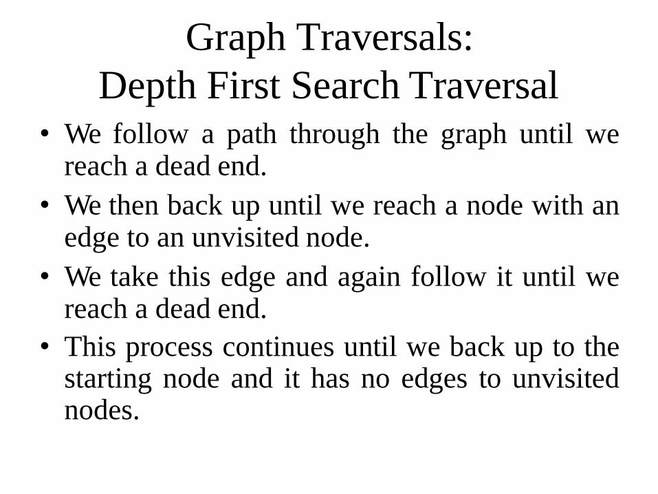
Depth First Search Traversal • We follow a path through the graph until we

reach a dead end.

• We then back up until we reach a node with an edge to an unvisited node.

• We take this edge and again follow it until we reach a dead end.

• This process continues until we back up to the starting node and it has no edges to unvisited nodes.

Depth First Search Traversal

Example • Consider the following graph:

• The order of the depth-first traversal of this graph starting at node 1 would be: 1, 2, 3, 4, 7, 5, 6, 8, 9

Breadth First Search Traversal

• From the starting node, we follow all paths of length one.

• Then we follow paths of length two that go to unvisited nodes.

• We continue increasing the length of the paths until there are no unvisited nodes along any of the paths.

Breadth First Search Traversal

Example • Consider the following graph:

• The order of the breadth-first traversal of this graph starting at node 1 would be: 1, 2, 8, 3, 7, 4, 5, 9, 6

UNIT - 5

BINARY TREES AND HASHING

B.Padmaja

Associate Professor

Department of CSE


170

CONTENTS

• Binary Search Trees - Properties and

Operations

• Balanced Search Trees – AVL Trees

• M – way Search Trees

• B Trees

• Hashing – Hash Table, Hash Function

• Collisions

• Applications of Hashing

180

Binary Search Trees

• In a BST, each node stores some information

including a unique key value, and perhaps some

associated data. A binary tree is a BST iff, for every

node n in the tree:

• All keys in n's left subtree are less than the key in n,

and

• All keys in n's right subtree are greater than the key in

n.

• In other words, binary search trees are binary trees in

which all values in the node‘s left subtree are less

than node value all values in the node‘s right subtree

are greater than node value.

BST Example

190

191

Properties and Operations

A BST is a binary tree of nodes ordered in the

following way:

i. Each node contains one key (also unique)

ii. The keys in the left subtree are < (less) than the

key in its parent node

iii. The keys in the right subtree > (greater) than the

key in its parent node

iv. Duplicate node keys are not allowed.

192

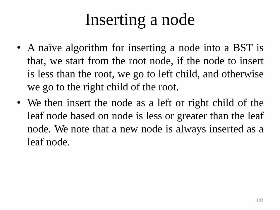
Inserting a node

• A naïve algorithm for inserting a node into a BST is

that, we start from the root node, if the node to insert

is less than the root, we go to left child, and otherwise

we go to the right child of the root.

• We then insert the node as a left or right child of the

leaf node based on node is less or greater than the leaf

node. We note that a new node is always inserted as a

leaf node.

193

Inserting a node

• A recursive algorithm for inserting a node into a

BST is as follows. Assume we insert a node N to

tree T. if the tree is empty, the we return new node

N as the tree. Otherwise, the problem of inserting

is reduced to inserting the node N to left of right

sub trees of T, depending on N is less or greater

than T. A definition is as follows.

Insert(N, T) = N if T is empty

= insert(N, T.left) if N < T

= insert(N, T.right) if N > T

194

Searching for a node

• Searching for a node is similar to inserting a node.

We start from root, and then go left or right until we

find (or not find the node). A recursive definition of

search is as follows. If the node is equal to root, then

we return true. If the root is null, then we return false.

Otherwise we recursively solve the problem for T.left

or T.right, depending on N < T or N > T. A recursive

definition is as follows.

• Search should return a true or false, depending on the

node is found or not.

= search(N, T.right) if N > T

Searching for a node • Search(N, T) = false if T is empty Searching for a node is

similar to inserting a node. We start from root, and then

go left or right until we find (or not find the node).

• A recursive definition of search is as follows. If the node

is equal to root, then we return true. If the root is null,

then we return false. Otherwise we recursively solve the

problem for T.left or T.right, depending on N < T or N >

T. A recursive definition is as follows.

• Search should return a true or false, depending on the

node is found or not.

Search(N, T) = false if T is empty

= true if T = N

= search(N, T.left) if N < T 186

Deleting a node

• A BST is a connected structure. That is, all nodes in a

tree are connected to some other node. For example,

each node has a parent, unless node is the root.

Therefore deleting a node could affect all sub trees of

that node. For example, deleting node 5 from the tree

could result in losing sub trees that are rooted at 1 and

9.

196

197

Balanced Search Trees

• A self-balancing (or height-balanced) binary search

tree is any node-based binary search tree that

automatically keeps its height (maximal number of levels

below the root) small in the face of arbitrary item

insertions and deletions.

• AVL Trees: An AVL tree is another balanced binary

search tree. Named after their inventors, Adelson-Velskii

and Landis, they were the first dynamically balanced

trees to be proposed. Like red-black trees, they are not

perfectly balanced, but pairs of sub-trees differ in height

by at most 1, maintaining an O(logn) search time.

Addition and deletion operations also take O(logn) time.

198

AVL Tree - Definition

• Definition of an AVL tree: An AVL tree is a binary

search tree which has the following properties:

i. The sub-trees of every node differ in height by at most one.

ii. Every sub-tree is an AVL tree.

• Balance requirement for an AVL tree: the left and right

sub-trees differ by at most 1 in height.

190

200

Balance Factor

• To implement our AVL tree we need to keep track of a

balance factor for each node in the tree. We do this by

looking at the heights of the left and right subtrees for

each node. More formally, we define the balance factor

for a node as the difference between the height of the

left subtree and the height of the right subtree.

balanceFactor=height(leftSubTree)−height(rightSubTree)

• Using the definition for balance factor given above we

say that a subtree is left-heavy if the balance factor is

greater than zero. If the balance factor is less than zero

then the subtree is right heavy. If the balance factor is

zero then the tree is perfectly in balance.

Balance Factor

201

Introduction to M-Way Search Trees

• A multiway tree is a tree that can have more than two

children. A multiway tree of order m (or an m-way tree)

is one in which a tree can have m children.

• As with the other trees that have been studied, the nodes

in an m-way tree will be made up of key fields, in this

case m-1 key fields, and pointers to children.

• Multiday tree of order 5

202

Properties of M-way Search Trees

• m-way search tree is a m-way tree in which:

i. Each node has m children and m-1 key fields

ii. The keys in each node are in ascending order.

iii. The keys in the first i children are smaller than the ith key

iv. The keys in the last m-i children are larger than the ith

key

• 4-way search tree

203

204

B -Trees • An extension of a multiway search tree of order m is a B-

tree of order m. This type of tree will be used when the

data to be accessed/stored is located on secondary storage

devices because they allow for large amounts of data to

be stored in a node.

• A B-tree of order m is a multiway search tree in which:

iii.

i. The root has at least two subtrees unless it is the only node in

the tree.

ii. Each nonroot and each nonleaf node have at most m nonempty

children and at least m/2 nonempty children.

The number of keys in each nonroot and each nonleaf node is

one less than the number of its nonempty children.

iv. All leaves are on the same level.

205

Searching a B -Tree

• Start at the root and determine which pointer to

follow based on a comparison between the search

value and key fields in the root node.

• Follow the appropriate pointer to a child node.

• Examine the key fields in the child node and

continue to follow the appropriate pointers until

the search value is found or a leaf node is reached

that doesn't contain the desired search value.

206

Insertion into a B -Tree

• The condition that all leaves must be on the same

level forces a characteristic behavior of B-trees,

namely that B-trees are not allowed to grow at the

their leaves; instead they are forced to grow at the

root.

• When inserting into a B-tree, a value is inserted

directly into a leaf. This leads to three common

situations that can occur:

i. A key is placed into a leaf that still has room.

ii. The leaf in which a key is to be placed is full.

iii. The root of the B-tree is full.

207

208

209

210

Deleting from a B -Tree

• The deletion process will basically be a reversal

of the insertion process - rather than splitting

nodes, it's possible that nodes will be merged so

that B-tree properties, namely the requirement

that a node must be at least half full, can be

maintained.

• There are two main cases to be considered:

i. Deletion from a leaf

ii. Deletion from a non-leaf

211

212

Hashing • Hashing is the technique used for performing almost

constant time search in case of insertion, deletion and find

operation.

• Taking a very simple example of it, an array with its

index as key is the example of hash table. So each index

(key) can be used for accessing the value in a constant

search time. This mapping key must be simple to compute

and must helping in identifying the associated value.

Function which helps us in generating such kind of key-

value mapping is known as Hash Function.

• In a hashing system the keys are stored in an array which

is called the Hash Table. A perfectly implemented hash

table would always promise an

insert/delete/retrieval time of O(1).

average 204

Hashing Function

• A function which employs some algorithm to computes

the key K for all the data elements in the set U, such that

the key K which is of a fixed size. The same key K can be

used to map data to a hash table and all the operations

like insertion, deletion and searching should be possible.

The values returned by a hash function are also referred

to as hash values, hash codes, hash sums, or hashes.

214

215

Hash Collision • A situation when the resultant hashes for two or

more data elements in the data set U, maps to the same

location in the has table, is called a hash collision. In such

a situation two or more data elements would qualify to be

stored / mapped to the same location in the hash table.

• Hash collision resolution techniques:

• Open Hashing (Separate chaining):Open Hashing, is a

technique in which the data is not directly stored at the

hash key index (k) of the Hash table. Rather the data at

the key index (k) in the hash table is a pointer to the head

of the data structure where the data is actually stored. In

the most simple and common implementations the data

structure adopted for storing the element is a linked-list.

216

217

Closed Hashing (Open Addressing)

• In this technique a hash table with pre-identified size

is considered. All items are stored in the hash table

itself. In addition to the data, each hash bucket also

maintains the three states: EMPTY, OCCUPIED,

DELETED. While inserting, if a collision occurs,

alternative cells are tried until an empty bucket is

found. For which one of the following technique is

adopted.

• Liner Probing

• Quadratic probing

• Double hashing

A Comparative Analysis of Closed

Hashing vs Open Hashing

218

210

Applications of Hashing

• A hash function maps a variable length input string to

fixed length output string -- its hash value, or hash for

short. If the input is longer than the output, then some

inputs must map to the same output -- a hash collision.

• Comparing the hash values for two inputs can give us one

of two answers: the inputs are definitely not the same, or

there is a possibility that they are the same. Hashing as we

know it is used for performance improvement, error

checking, and authentication.

• In error checking, hashes (checksums, message digests,

etc.) are used to detect errors caused by either hardware or

software. Examples are TCP checksums, ECC memory,

and MD5 checksums on downloaded files.

211

Applications of Hashing

• Construct a message authentication code (MAC)

• Digital signature

• Make commitments, but reveal message later

• Timestamping

• Key updating: key is hashed at specific intervals

resulting in new key

THANK YOU

Documents

UNIT - 1 INTRODUCTION TO DATA STRUCTURES, SEARCHING … · Simple and Compound Data Structures •Simple Data Structure: Simple data structure can be constructed with the help of