Unit-05/Lecture-01

Pipeline Processing

In computing, a pipeline is a set of data processing elements connected in series, where the output of

one element is the input of the next one. The elements of a pipeline are often executed in parallel or

in time-sliced fashion; in that case, some amount of buffer storage is often inserted between

elements.

Computer-related pipelines include:

Instruction pipelines, such as the classic RISC pipeline, which are used in central processing

units (CPUs) to allow overlapping execution of multiple instructions with the same circuitry.

The circuitry is usually divided up into stages, including instruction decoding, arithmetic, and

register fetching stages, wherein each stage processes one instruction at a time.

Graphics pipelines, found in most graphics processing units (GPUs), which consist of multiple

arithmetic units, or complete CPUs, that implement the various stages of common rendering

operations (perspective projection, window clipping, color and light calculation, rendering,

etc.).

Software pipelines, where commands can be written where the output of one operation is

automatically fed to the next, following operation. The Unix system call pipe is a classic

example of this concept, although other operating systems do support pipes as well.

Pipelining is a natural concept in everyday life, e.g. on an assembly line. Consider the assembly of a car:

assume that certain steps in the assembly line are to install the engine, install the hood, and install the

wheels (in that order, with arbitrary interstitial steps). A car on the assembly line can have only one of

the three steps done at once. After the car has its engine installed, it moves on to having its hood

installed, leaving the engine installation facilities available for the next car. The first car then moves on

to wheel installation, the second car to hood installation, and a third car begins to have its engine

installed. If engine installation takes 20 minutes, hood installation takes 5 minutes, and wheel

installation takes 10 minutes, then finishing all three cars when only one car can be assembled at once

would take 105 minutes. On the other hand, using the assembly line, the total time to complete all

we dont take any liability for the notes correctness. http://www.rgpvonline.com

three is 75 minutes. At this point, additional cars will come off the assembly line at 20 minute

increments.

Linear and non-linear pipelines

A linear pipeline processor is a series of processing stages which are arranged linearly to perform a

specific function over a data stream. The basic usages of linear pipeline is instruction execution,

arithmetic computation and memory access.

A non linear pipelining (also called dynamic pipeline) can be configured to perform various functions at

different times. In a dynamic pipeline there is also feed forward or feedback connection. Non-linear

pipeline also allows very long instruction word.

Fig 5.1

As the assembly-line example shows, pipelining doesn't decrease the time for processing a single

datum; it only increases the throughput of the system when processing a stream of data.

"High" pipelining leads to increase of latency - the time required for a signal to propagate through a

full pipe.

A pipelined system typically requires more resources (circuit elements, processing units, computer

memory, etc.) than one that executes one batch at a time, because its stages cannot reuse the

resources of a previous stage. Moreover, pipelining may increase the time it takes for an instruction to

finish.

we dont take any liability for the notes correctness. http://www.rgpvonline.com

RGPV QUESTIONS Year Marks

Q.1 Draw a four segment pipeline June 2014 2

Q.2 Formulate a six segment instruction pipeline for a

computer. Specify the operation to be performed in each

segment.

June 2012 7

Q.3 What is pipelining? What is the need of pipelining? Explain

the pipeline organization of an arithmetic pipelines

Dec 2011 7

we dont take any liability for the notes correctness. http://www.rgpvonline.com

Unit-05/Lecture-02

Vector Processing

A Vector processor, or array processor, is a central processing unit (CPU) that implements an

instruction set containing instructions that operate on one-dimensional arrays of data called vectors.

This is in contrast to a scalar processor, whose instructions operate on single data items. Vector

processors can greatly improve performance on certain workloads, notably numerical simulation and

similar tasks. Vector machines appeared in the early 1970s and dominated supercomputer design

through the 1970s into the 90s, notably the various Cray platforms. The rapid fall in the price-to-

performance ratio of conventional microprocessor designs led to the vector supercomputer's demise

in the later 1990s.

Today, most commodity CPUs implement architectures that feature instructions for a form of vector

processing on multiple (vectorized) data sets, typically known as SIMD (Single Instruction, Multiple

Data). Common examples include VIS, MMX, SSE, AltiVec and AVX. Vector processing techniques are

also found in video game console hardware and graphics accelerators. In 2000, IBM, Toshiba and

Sony collaborated to create the Cell processor, consisting of one scalar processor and eight vector

processors, which found use in the Sony PlayStation 3 among other applications.

Other CPU designs may include some multiple instructions for vector processing on multiple

(vectorised) data sets, typically known as MIMD (Multiple Instruction, Multiple Data) and realized

with VLIW. Such designs are usually dedicated to a particular application and not commonly

marketed for general purpose computing. In the Fujitsu FR-V VLIW/vector processor both

technologies are combined.

or

Vector processing was once intimately associated with the concept of a "supercomputer". As with

most architectural techniques for achieving high performance, it exploits regularities in the structure

of computation, in this case, the fact that many codes contain loops that range over linear arrays of

data performing symmetric operations.

we dont take any liability for the notes correctness. http://www.rgpvonline.com

The origins of vector architecure lay in trying to address the problem of instruction bandwidth. By

the end of the 1960's, it was possible to build multiple pipelined functional units, but the fetch and

decode of instructions from memory was too slow to permit them to be fully exploited. Applying a

single instruction to multiple data elements (SIMD) is one simple and logical way to leverage limited

instruction bandwidth.

The most powerful computers of the 1970s and 1980s tended to be vector machines, from Cray,

NEC, and Fujitsu, but with increasingly higher degrees of semiconductor integration, the mismatch

between instruction bandwidth and operand bandwidth essentially went away. As of 2009, only 1 of

the worlds top 500 supercomputers was still based on a vector architecture.

The lessons of SIMD processing weren't entirely lost, however. While Cray-style vector units that

perform a common operations across vector registers of hundreds or thousands of data elements

have largely disappeared, the SIMD approach has been applied to the processing of 8 and 16-bit

multimedia data by 32 and 64-bit processors and DSPs with great success. Under the names "MMX"

and "SSE", SIMD processing can be found in essentially every modern personal computer, where it is

exploited by image processing and audio applications.

RGPV QUESTIONS Year Marks

Q.1 Give definition of vector processing .And enlist its

application

June 2014 2

Q.2 What does pipeline , vector and array processors mean in

parallel processing?

June 2011 10

Q.3 Explain any one vector processing method with suitable

illustration

Dec 2010 4

we dont take any liability for the notes correctness. http://www.rgpvonline.com

Unit-05/Lecture-03

Instruction pipelining

An instruction pipeline is a technique used in the design of computers to increase their instruction

throughput (the number of instructions that can be executed in a unit of time). The basic instruction

cycle is broken up into a series called a pipeline. Rather than processing each instruction sequentially

(one at a time, finishing one instruction before starting the next), each instruction is split up into a

sequence of steps so different steps can be executed concurrently (at the same time) and in parallel

(by different circuitry).

Pipelining increases instruction throughput by performing multiple operations at the same time

(concurrently), but does not reduce instruction latency (the time to complete a single instruction from

start to finish) as it still must go through all steps. Indeed, it may increase latency due to additional

overhead from breaking the computation into separate steps and worse, the pipeline may stall (or

even need to be flushed), further increasing latency. Pipelining thus increases throughput at the cost

of latency, and is frequently used in CPUs, but avoided in realtime systems, where latency is a hard

constraint.

Each instruction is split into a sequence of dependent steps. The first step is always to fetch the

instruction from memory; the final step is usually writing the results of the instruction to processor

registers or to memory. Pipelining seeks to let the processor work on as many instructions as there are

dependent steps, just as an assembly line builds many vehicles at once, rather than waiting until one

vehicle has passed through the line before admitting the next one. Just as the goal of the assembly line

is to keep each assembler productive at all times, pipelining seeks to keep every portion of the

processor busy with some instruction. Pipelining lets the computer's cycle time be the time of the

slowest step, and ideally lets one instruction complete in every cycle.

The term pipeline is an analogy to the fact that there is fluid in each link of a pipeline, as each part of

the processor is occupied with work.

we dont take any liability for the notes correctness. http://www.rgpvonline.com

Central processing units (CPUs) are driven by a clock. Each clock pulse need not do the same thing;

rather, logic in the CPU directs successive pulses to different places to perform a useful sequence.

There are many reasons that the entire execution of a machine instruction cannot happen at once. For

example, if one clock pulse latches a value into a register or begins a calculation, it will take some time

for the value to be stable at the outputs of the register or for the calculation to complete. As another

example, reading an instruction out of a memory unit cannot be done at the same time that an

instruction writes a result to the same memory unit. In pipelining, effects that cannot happen at the

same time are made the dependent steps of the instruction.

Number of steps

The number of dependent steps varies with the machine architecture. For example:

The IBM Stretch project proposed the terms Fetch, Decode, and Execute that have become common.

The classic RISC pipeline comprises:

Instruction fetch

Instruction decode and register fetch

Execute

Memory access

Register write back

The Atmel AVR and the PIC microcontroller each have a 2-stage pipeline.

Many designs include pipelines as long as 7, 10 and even 20 stages (as in the Intel Pentium 4).

The later "Prescott" and "Cedar Mill" Pentium 4 cores (and their Pentium D derivatives) had a 31-stage

we dont take any liability for the notes correctness. http://www.rgpvonline.com

pipeline, the longest in mainstream consumer computing.

The Xelerated X10q Network Processor has a pipeline more than a thousand stages long.

As the pipeline is made "deeper" (with a greater number of dependent steps), a given step can be

implemented with simpler circuitry, which may let the processor clock run faster.[2] Such pipelines

may be called superpipelines.

A processor is said to be fully pipelined if it can fetch an instruction on every cycle. Thus, if some

instructions or conditions require delays that inhibit fetching new instructions, the processor is not

fully pipelined

we dont take any liability for the notes correctness. http://www.rgpvonline.com

Unit-05/Lecture-04

Arithmetic Pipeline

As pipelining techniques developed, it became clear that pipelining the hardware used to implement

complex arithmetic operations such as floating-point addition and multiplication could enhance

performance. Floating-point addition, for example, consists of four distinct operations (exponent

subtraction, mantissa shifting, mantissa addition, normalisation) which can be pipelined in a very

straightforward manner.

In a one-address system no benefit would be gained from pipelining arithmetic opreations: since one

of the input operands to an addition operation in a one-address system is always the Accumulator, it

cannot be used as an input to a subsequent operation until the current operation has finished. This

implies that temporal overlap of two successive additions is not possible if the result must always pass

through the Accumulator. For successful operation of a pipelined arithmetic unit each instruction must

reference at least two and preferably three operands.

Each AU was made up of eight distinct sections, each of which performed a separate arithmetic or

logical operation (see figure). Each section could be connected to any other section to allow the

correct sequence of operations to be executed for a particular instruction, with the appropriate

configuration being established at the start of a vector instruction. In any given configuration the

various sections formed a pipeline into which a new pair of operands could, in principle, be entered at

each 60 ns clock, and after a start-up time, corresponding to as many clock periods as there were

sections in use, result operands emerged at a rate of one per clock period. At the end of a vector

instruction there was a similar run-down time between the entry of the last operand pair and the

emergence of the corresponding result.

Floating-point addition, for example, required the use of the Receiver Register, Exponent Subtract,

Align, Add, Normalise and Output sections, connected as shown by the solid line in the figure. Pairs of

operands from the MBU were first copied into the Receiver Register, the cable delays between the

MBU and AU effectively forming a complete stage in the overall pipeline arrangement. The Exponent

Subtract section then performed a 7-bit subtraction to determine the difference between the

we dont take any liability for the notes correctness. http://www.rgpvonline.com

exponents of the two floating-point operands, or in the case of equal exponents, used logic to

determine which of the fractional mantissae was larger (this logic was also used by those instructions

that tested for greater than, less than or equal to, in order to avoid duplication of hardware).

The exponent difference was used in the Align section to shift right the mantissa of the operand with

the smaller exponent. In one cycle any shift which was a multiple of four could be carried out, this

being all that is required for floating-point numbers represented in base 16. (Fixed-point right shifts

required two cycles, one shifting by the largest multiple of four in the shift value, and a second in

which the result of the first was re-entered and shifted by the residue of 0, 1, 2 or 3.)

Having been correctly aligned, the fractional parts of the two floating-point numbers were added in

the Add section, and the result passed on to the Normalise section. This section closely resembled the

Align section in that floating-point operations only required one cycle, while the fixed-point left shifts

which it also carried out required two. The major difference between these two sections was that

Align received information concerning the length of shift required in floating-point operations, while

the Normalise section had to compute the shift length by determining which four-bit group contained

the most significant digit. It also contained an adder to update the exponent value when a

normalisation shift occured. The results of all arithmetic operations passed through the Output section

before being returned to the Memory Buffer Unit. The partitioning of the arithmetic unit into these

various sections was primarily intended to give high throughput of floating-point addition and

subtraction. Each section was capable of operating on double length operands so that vector double

length instructions could proceed at the clock rate. Double length multiplication, and all divides (which

were performed by an iterative technique), proceeded more slowly.

The dashed line in the figure shows the interconnection used for fixed-point multiplication. The

Multiply section could perform a 32 by 32-bit multiplication in one clock period, so that the results of

both fixed-point and single-length floating-point multiplication were available after one pass through

the multiplier. Because a carry-save addition technique was used, the output of the Multiply section

consisted of a 64-bit pseudo-sum and a 64-bit pseudo-carry. These were added in the Add unit to

produce the true result. Double-length multiplication required three separate 32 by 32-bit

multiplications to be performed and these could therefore proceed at a rate of only one every three

clocks. After passing through the Add section the three separate results were added together in their

we dont take any liability for the notes correctness. http://www.rgpvonline.com

proper bit positions in the Accumulate section.

The Accumulate section was similar to the Add section and was used in all instructions which required

a running total to be maintained. An important example of this type of instruction is the Vector Dot

Product, which is used repeatedly, for example, in matrix multiplication. Pairs of operands are

multiplied together in this instruction and a single scalar result, equal to the sum of the products of

the pairs, is produced. Because the running total was maintained in the arithmetic unit, the read after

write problems which occur in scalar implementations of this operation were avoided in the ASC.

Fig 5.2 Floating Point Airthmetic Pipeline

we dont take any liability for the notes correctness. http://www.rgpvonline.com

Fig 5.3 Pipelined Multiplication using Carry Save Addition

RGPV QUESTIONS Year Marks

Q.1 Differentiate instruction and arithmetic pipeline June 2014 7

Q.2 Draw and explain the pipeline for floating point addition

and subtraction

June 2011 10

we dont take any liability for the notes correctness. http://www.rgpvonline.com

Unit-05/Lecture-05

Vector processors

A vector processor, or array processor, is a central processing unit (CPU) that implements an

instruction set containing instructions that operate on one-dimensional arrays of data called vectors.

This is in contrast to a scalar processor, whose instructions operate on single data items. Vector

processors can greatly improve performance on certain workloads, notably numerical simulation and

similar tasks. Vector machines appeared in the early 1970s and dominated supercomputer design

through the 1970s into the 90s, notably the various Cray platforms. The rapid fall in the price-to-

performance ratio of conventional microprocessor designs led to the vector supercomputer's demise

in the later 1990s.

Today, most commodity CPUs implement architectures that feature instructions for a form of vector

processing on multiple (vectorized) data sets, typically known as SIMD (Single Instruction, Multiple

Data). Common examples include VIS, MMX, SSE, AltiVec and AVX. Vector processing techniques are

also found in video game console hardware and graphics accelerators. In 2000, IBM, Toshiba and Sony

collaborated to create the Cell processor, consisting of one scalar processor and eight vector

processors, which found use in the Sony PlayStation 3 among other applications.

Other CPU designs may include some multiple instructions for vector processing on multiple

(vectorised) data sets, typically known as MIMD (Multiple Instruction, Multiple Data) and realized with

VLIW. Such designs are usually dedicated to a particular application and not commonly marketed for

general purpose computing. In the Fujitsu FR-V VLIW/vector processor both technologies are

combined.

or

Vector processors are special purpose computers that match a range of (scientific) computing tasks.

These tasks usually consist of large active data sets, often poor locality, and long run times. In addition,

we dont take any liability for the notes correctness. http://www.rgpvonline.com

vector processors provide vector instructions.

These instructions operate in a pipeline (sequentially on all elements of vector registers), and in

current machines. Some properties of vector instructions are

__The computation of each result is independent of the computation of previous results, allowing a

very deep pipeline without any data hazards.

__A single vector instruction specifies a tremendous amount of work – it is the same as executing an

entire loop. Thus, the instruction bandwidth requirement is reduced.

__Vector instructions that access memory have a known access pattern. If the vector elements are all

adjacent, then fetching the vector from a set of heavily interleaved memory banks works very well.

Because a single access is initiated for the entire vector rather than to a single word, the high latency

of initiating a main memory access versus accessing a cache is amortized. Thus, the cost of the latency

to main memory is seen only once for the entire vector, rather than once for each word of the vector.

__Control hazards are non-existent because an entire loop is replaced by a vector instruction whose

behavior is predetermined.

Typical vector operations include (integer and floating point:

__Add two vectors to produce a third.

__Subtract two vectors to produce a third

__Multiply two vectors to produce a third

__Divide two vectors to produce a third

__Load a vector from memory

__Store a vector to memory.

These instructions could be augmented to do typical array operations:

we dont take any liability for the notes correctness. http://www.rgpvonline.com

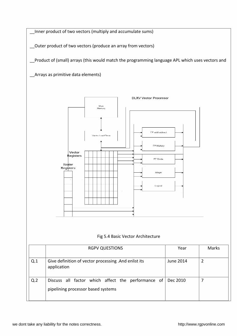
__Inner product of two vectors (multiply and accumulate sums)

__Outer product of two vectors (produce an array from vectors)

__Product of (small) arrays (this would match the programming language APL which uses vectors and

__Arrays as primitive data elements)

Fig 5.4 Basic Vector Architecture

RGPV QUESTIONS Year Marks

Q.1 Give definition of vector processing .And enlist its

application

June 2014 2

Q.2 Discuss all factor which affect the performance of

pipelining processor based systems

Dec 2010 7

we dont take any liability for the notes correctness. http://www.rgpvonline.com

Unit-05/Lecture-06

Array processor

Array processor A computer/processor that has an architecture especially designed for processing arrays (e.g.

matrices) of numbers. The architecture includes a number of processors (say 64 by 64) working simultaneously,

each handling one element of the array, so that a single operation can apply to all elements of the array in

parallel. To obtain the same effect in a conventional processor, the operation must be applied to each element

of the array sequentially, and so consequently much more slowly.

An array processor may be built as a self-contained unit attached to a main computer via an I/O port or internal

bus; alternatively, it may be a distributed array processor where the processing elements are distributed

throughout, and closely linked to, a section of the computer's memory.

Array processors are very powerful tools for handling problems with a high degree of parallelism. They do

however demand a modified approach to programming. The conversion of conventional (sequential) programs

to serve array processors is not a trivial task, and it is sometimes necessary to select different (parallel)

algorithms to suit the parallel approach.

Or

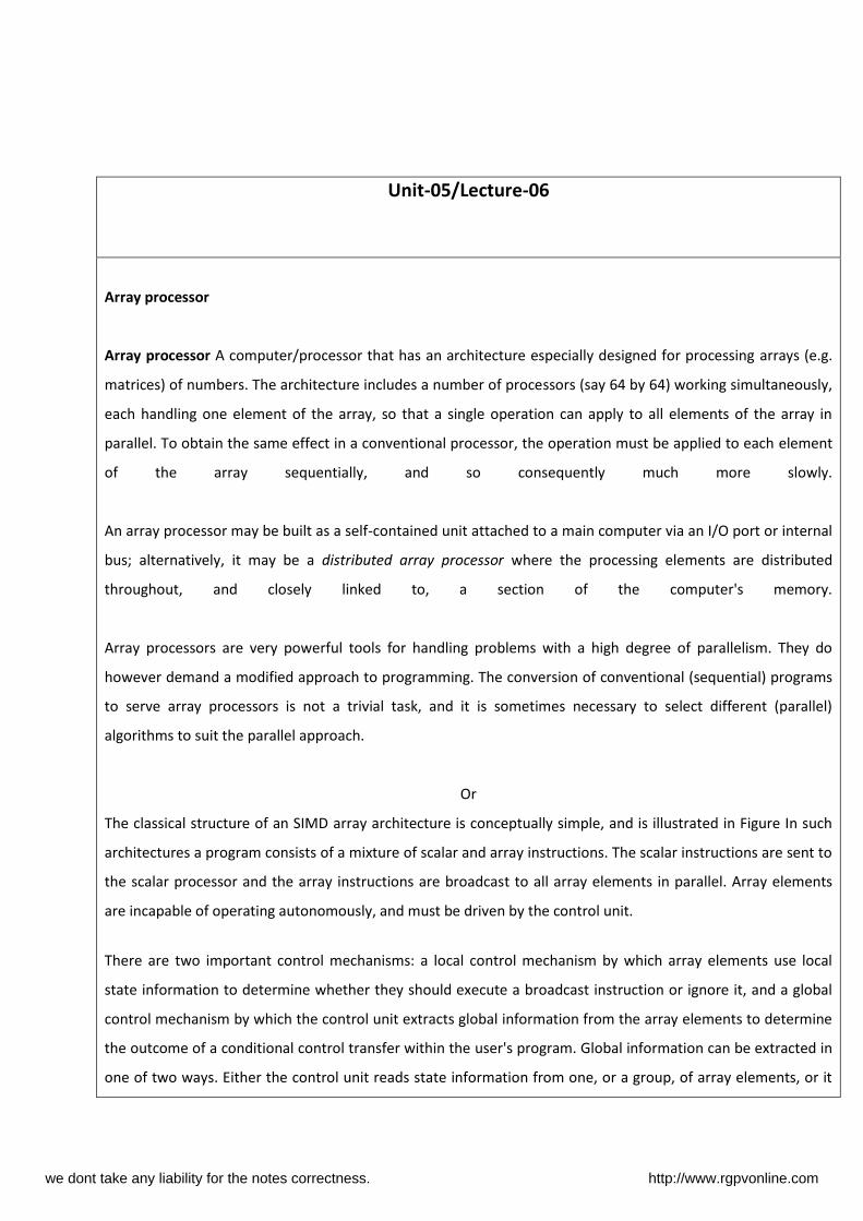
The classical structure of an SIMD array architecture is conceptually simple, and is illustrated in Figure In such

architectures a program consists of a mixture of scalar and array instructions. The scalar instructions are sent to

the scalar processor and the array instructions are broadcast to all array elements in parallel. Array elements

are incapable of operating autonomously, and must be driven by the control unit.

There are two important control mechanisms: a local control mechanism by which array elements use local

state information to determine whether they should execute a broadcast instruction or ignore it, and a global

control mechanism by which the control unit extracts global information from the array elements to determine

the outcome of a conditional control transfer within the user's program. Global information can be extracted in

one of two ways. Either the control unit reads state information from one, or a group, of array elements, or it

we dont take any liability for the notes correctness. http://www.rgpvonline.com

senses a boolean control line representing the logical OR (or possibly the logical AND) of a particular local state

variable from every array element.

The three major components of an array structure are the array units, the memory they access, and the

connections between the two. There are two ways in which these components can be organised. Figure 2

shows the basic structure of an array processor in which memory is shared between the array elements and

Figure 3 illustrates the basic structure of an array processor in which all memory is distributed amongst the

array elements.

If all memory is shared then the switch network connecting the array units to the memory must be capable of

sustaining a high rate of data transfer, since every instruction will require massive movement of data between

these two components. Alternatively, if the memory is distributed then the majority of operands will hopefully

reside within the local memory of each processing element (where processing element = arithmetic unit +

memory module), and a much lower performance from the switch network can be tolerated. The design of the

switch network is of central importance, a topic is covered in the section on Networks.

Early examples of these two styles of array processor architecture were the highly influential ILLIAC IV machine,

which had a fully distributed memory, and the ill-fated Burroughs Scientific Processor (BSP), which had a shared

memory.

Fig 5.5 Classical SIMD Array Architecture

we dont take any liability for the notes correctness. http://www.rgpvonline.com

Fig 5. 6 Array processor with Shared Memory

Fig 5.7 Array Processor with Distributed Memory

RGPV QUESTIONS Year Marks

Q.1 Draw and explain the typical functional structure of a SIMD

array processor.

June 2011

June 2012

10

Q.2 Draw a space time diagram of a six segment pipeline

showing the time it takes to process eight tasks

June 2014 7

we dont take any liability for the notes correctness. http://www.rgpvonline.com

Unit-05/Lecture-07

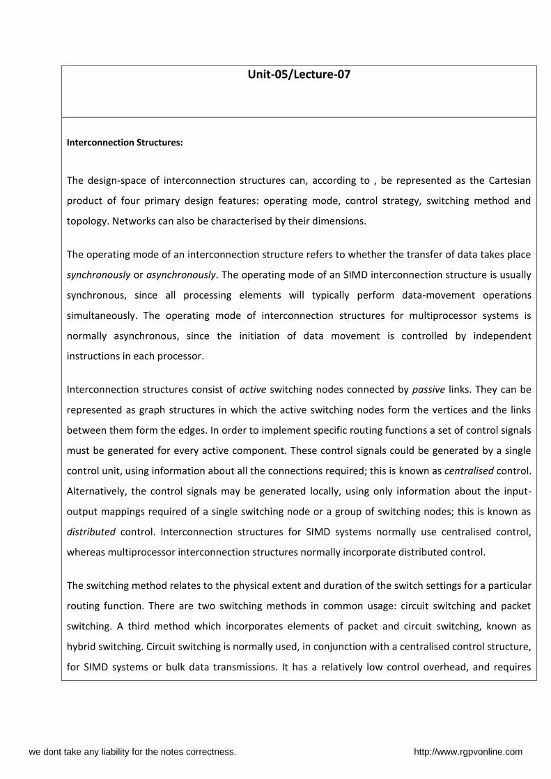
Interconnection Structures:

The design-space of interconnection structures can, according to , be represented as the Cartesian

product of four primary design features: operating mode, control strategy, switching method and

topology. Networks can also be characterised by their dimensions.

The operating mode of an interconnection structure refers to whether the transfer of data takes place

synchronously or asynchronously. The operating mode of an SIMD interconnection structure is usually

synchronous, since all processing elements will typically perform data-movement operations

simultaneously. The operating mode of interconnection structures for multiprocessor systems is

normally asynchronous, since the initiation of data movement is controlled by independent

instructions in each processor.

Interconnection structures consist of active switching nodes connected by passive links. They can be

represented as graph structures in which the active switching nodes form the vertices and the links

between them form the edges. In order to implement specific routing functions a set of control signals

must be generated for every active component. These control signals could be generated by a single

control unit, using information about all the connections required; this is known as centralised control.

Alternatively, the control signals may be generated locally, using only information about the input-

output mappings required of a single switching node or a group of switching nodes; this is known as

distributed control. Interconnection structures for SIMD systems normally use centralised control,

whereas multiprocessor interconnection structures normally incorporate distributed control.

The switching method relates to the physical extent and duration of the switch settings for a particular

routing function. There are two switching methods in common usage: circuit switching and packet

switching. A third method which incorporates elements of packet and circuit switching, known as

hybrid switching. Circuit switching is normally used, in conjunction with a centralised control structure,

for SIMD systems or bulk data transmissions. It has a relatively low control overhead, and requires

we dont take any liability for the notes correctness. http://www.rgpvonline.com

relatively simple switching nodes.

Packet switching is most commonly used in multiprocessor and other MIMD systems, or where short

bursts of data transmission are required. The packets are normally self-routing, requiring complex

switching nodes; often under distributed control. Routing conflicts are possible when self-routing

packets are used, and this in turn requires a conflict resolution strategy. Examples of conflict

resolution strategies can be found under Shared Memory Multiprocessors.

Fig 5.8 Interconnection Structures

we dont take any liability for the notes correctness. http://www.rgpvonline.com

Unit-05/Lecture-08

Inter-process communication (IPC)

Inter-process communication (IPC) is the activity of sharing data across multiple and commonly

specialized processes using communication protocols. Typically, applications using IPC are categorized

as clients and servers, where the client requests data and the server responds to client requests.[1]

Many applications are both clients and servers, as commonly seen in distributed computing. Methods

for achieving IPC are divided into categories which vary based on software requirements, such as

performance and modularity requirements, and system circumstances, such as network bandwidth

and latency.

There are several reasons for implementing inter-process communication systems:

Sharing information; for example, web servers use IPC to share web documents and media

with users through a web browser.

Distributing labor across systems; for example, Wikipedia uses multiple servers that

communicate with one another using IPC to process user requests.[2]

Privilege separation; for example, HMI software systems are separated into layers based on

privileges to minimize the risk of attacks. These layers communicate with one another using

encrypted IPC.

Fig 5.9

we dont take any liability for the notes correctness. http://www.rgpvonline.com

RGPV QUESTIONS Year Marks

Q.1 Explain the following terms:

(i)Pipeline conflicts

(ii) interproccessor communication

(iii)Interconnection structure

June 2012 7

.

we dont take any liability for the notes correctness. http://www.rgpvonline.com

Unit-05/Lecture-09

Inter-process communication (IPC)

Inter-process communication (IPC) is a mechanism that allows the exchange of data between

processes. By providing a user with a set of programming interfaces, IPC helps a programmer organize

the activities among different processes. IPC allows one application to control another application,

thereby enabling data sharing without interference.

IPC enables data communication by allowing processes to use segments, semaphores, and other

methods to share memory and information. IPC facilitates efficient message transfer between

processes. The idea of IPC is based on Task Control Architecture (TCA). It is a flexible technique that

can send and receive variable length arrays, data structures, and lists. It has the capability of using

publish/subscribe and client/server data-transfer paradigms while supporting a wide range of

operating systems and languages.

Or

Inter-Processor Communication (IPC) is a set of methods of exchanging data between two processors.

These two processors can be any combination of application processors, baseband processors,

connectivity processors and/or media processors. The most common examples of IPC use is dual mode

phones and data cards. Processors are not designed to talk to each other. Most interfaces found in

processors are masters or host controllers, such as I²C master, SPI master, and SDIO host controller.

The master and host controller need to connect to a slave or a client controller.

QuickLogic’s IPC technology provides system designers a quick and easy method to build a common

communication scheme between two processors. There are two types of architecture available for the

designer to choose from:

we dont take any liability for the notes correctness. http://www.rgpvonline.com

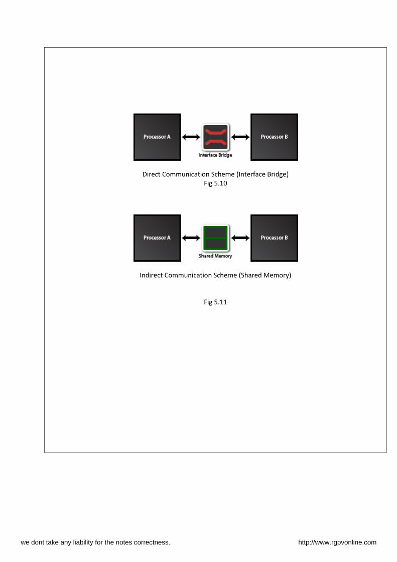
Direct Communication Scheme (Interface Bridge)

Fig 5.10

Indirect Communication Scheme (Shared Memory)

Fig 5.11

we dont take any liability for the notes correctness. http://www.rgpvonline.com