Uniqueness of a class of nonlinear electrostatic field problems

A.T.de Hoop and 1.E.Lager

Abstract: The uniqueness properties of a class of nonlinear electrostatic field problems are investigated. The study was motivated by the development of numerical algorithms to analyse the performance of nonlinear semiconducting electron devices. Here, existence and uniqueness of the solution are prerequisites for the numerical results to have any meaning at all.

1 Introduction

Theoretical methods to analyse electrostatic field problems of the type that occur in nonlinear dielectric or nonlinear semiconducting electron devices invariably make use of computational techniques of an iterative nature. Even if a particular technique of this kind proves to converge numer- ically to a certain answer, the question remains whether this answer is the correct one and not depending on the particu- lar numerical algorithm (including its starting values) employed. A possible ambiguity of this nature can only he resolved if the problem at hand can be shown to have a unique solution. For the case of linear media, the unique- ness properties of the solution of electromagnetic field problems in general have been studied extensively in the lit- erature (see, for example, [I] for dynamic fields and [2, 31 for static and stationary fields). All these proofs essentially rely on the use of the superposition principle. In the pres- ence of nonlinear media, however, the governing equations become nonlinear and the superposition principle fails to hold.

No general uniqueness proof for the solution of the elec- tromagnetic field equations in the case of arbitrarily nonlin- ear media seems to exist. Sufficient conditions for uniqueness can only be derived for certain classes of proh- lems for which additional assumptions as regards the con- stitutive properties of the media involved are made.

In this paper we shall present some criteria that ensure the uniqueness of the solution of a class of problems that refer to the computation of electrostatic fields of the type that occurs in nonlinear dielectric and nonlinear semicon- ducting electron devices. The relevant criteria are applicable to a wide range of problems met in electrical and electronic engineering practice.

The configurations to be considered are inhomogeneous in their electrical constitution, with possible jump disconti-

OIEE, 1999 IEE procredhfi~ online no. 19990491 DOT IO. IMY/ipsmt:1999019 I P a p fmt reaived 18Ih September 1998 and in revised foim 19th Apnl 1999

LE. Lager li with the International R-rch Centre for Tclmmulucations- trm&iion and Radar, Facully of ldomtion Tmhology and Systems, Den UluverSity of Technology, Mckclwcg 4 , 2 6 2 CD DelfI, The Netherlands

IEE Proc.~Sci. M e u Teclmol., Vol. 146, No 4. J u b 1999

nuities in their constitutive properties. They can he acti- vated by a variety of ‘external’ means. Included are, in this respect, the presence of ‘impressed’ electric volume charges and ‘impressed‘ electric polarisation. Of the former, we mention as an example the electric charges that are due to mechanical friction, accumulate in insulating parts of a configuration, and then can give rise to electrostatic dis- charges (ESDs). An example of the latter are objects con- sisting of permanently electrically polarised ceramics (electrets). Electric polarisation can also bc used to repre- sent the electrochemical action of a battery. In addition, ihe configuration can be excited electrically via a finite number of electrodes to which ‘external’ electric potentials are applied (as in the measuring equipment for electric capaci- tance tomography). It is important to notice that, due to the nonlinearity in the configuration’s electrical behaviour, the fields associated with these different excitation mecha- nisms cannot be constructed with the aid of the superposi- tion principle (as would be a natural way to do in the case of a configuration with linear electrical properties).

A rather detailed description is given of the admissible class of inhomogeneity and the admissible distributions in space of the source quantities. This description is not only necessary for stating the uniqueness theorem and construct- ing its proof, but it also serves as a guideline as to what fea- tures are to be accommodated in a numerical algorithm for solving field problems of the kind under consideration.

Most of the conditions that are invoked are sufficient conditions that have to do with existence of solutions of the partial differential equations and the associated boundary conditions involved (although we refrain from entering into the difficult area of existence proofs themselves), the appli- cability of Gauss’ divergence theorem, and the kind of con- ditions for uniqueness. Moreover, some emphasis is placed on the so-called ‘compatibility relations’ (the term stems from the theory of elasticity, [4], p. 49). These arc conse- quential relations that are automatically satisfied by any exact solution to the problem. However, as soon as solu- tions are constructed with the aid of numerical algorithms (which is almost a necessity in the case of nonlinear prob- lems), a compatibility relation is no longer automatically satisfied. Experience with the computation of both dynamic and static electromagnetic fields has shown that a numeri- cal solution can fail to converge and be highly erroneous if the relevant compatibility relations are not (numerically) taken into account as separate (and independent) condi-

175

tions [5, 61. A clear explanation for this phenomenon is not yet known, hut the facts are there.

The cases for configurations of hounded extent (where the field exterior to the configuration is negligibly small), as in a large class of (shielded) electronic devices, and for con- figurations embedded in a vacuum exterior domain (where the exterior field extends to infinity) will be investigated separately.

2 Formulation of field problem

In the formulation of the problem, the following constitu- ents are distinguished: the description of the configuration, the nomenclature of the field quantities, the nomenclature of the impressed volume source quantities, the (partial dif- ferential) field equations, the specification of the interface boundary conditions and the boundary conditions at the electrodes, and the description of the pertaining constitutive operators. As a corollary, the compatibility relation associ- ated with the field equations is given.

2.7 Description of Configuration The configuration to be analysed is present in thret-dimen- sional Euclidean space R3. Position in this space is specified by the Cartesian position vector Y . The material parts of the devices to be considered are contained in a bounded sub- domain D of R3. The boundary surface of 2, is denoted as dD. The (unbounded) complement of D U d'D in RS is the vacuum domain denoted as D". The domain D is parti- tioned into a, presumably finite, number N ( N 2 1) of suh- domains Da, n = 1, ._., N, in such a manner that, in the interior of each DB, the impressed volume source densities values and the constitutive operators are continuous func- tions of position (Cartesian scalar, vector or tensor func- tions, as appropriate), while their limiting values on approaching the closed boundary surface dDn of Dn via its interior are assumed to exist. Then, the only admissible dis- continuities are jump discontinuities which may occur across common interfaces between adjacent subdomains of D and/or at interfaces of the latter with D". The hounday surfaces dD and &!I,,, n = 1, ..., N, are assumed to be piece- wise smooth.

Furthermore, in D a finite number M + 1 (M 2 1) of dis- joint electrodes, occupying the surfaces S,, m = 0, 1, .._, M, is present. Through them, the configuration is electrically accessible for acting as an electric or electronic device. Each S,, is assumed to he either a closed surface or a two-sided, non-closed surface of vanishing thickness. For both cases, the surfaces are assumed to be piecewise smooth. For closed electrode surfaces, their interior is excluded from D. In the special case of a perfectly shielded configuration, we take So = aD, in which case the interior of S, coincides with D, while now D" plays no role in the analysis.

2.2 Impressed volume source quantities The impressed volume source quantities are: the impressed electric polarisation P m p = P"P(r) and, the impressed vol- ume source density of electric charge ,@"" = @'"''(P). Here, P"P(u) is assumed to be a piecewise continuous vector function of position, PmP having the bounded support DP C D, while p'"'p(v) is assumed to be a piecewise continuous scalar function of position, p " P having the bounded sup- port ZIP C D.

2.3 Electrostatic field quantities The field quantities that characterise the electrostatic field are: the electric potential @ = @(U), the electric field strength E = E(u), the electric flux density D = D(u) and the volume

176

density of charge p = &U). Under the assumptions stated in Subsections 2.1 and 2.2, it may be conjectured that there exists a solution to the field problem, in which the field quantities are continuously differentiable throughout each subdomain D,t, n = 1, ..., N, (and D", if applicable), while their limiting values on approaching the closed boundary surface aD,* of each subdomain Dn. via its interior, exist. The relevant existence proof is hard to give and is beyond the scope of the present paper.

2.4 Field equations In any subdomain Dn, n = 1, ..., N, of the configuration and D", the field quantities are to satisfy the partial differ- ential equations

and

The total electric field strength E consists of the already specified (field-value independent) impressed part l?"P = -q- l Pmp (active part) and a (field-value dependent) induced part End (passive part), i.e.

-O@(r) = E(r ) (1)

v . D(r) = p ( r ) (2)

E(r) = E'"'(r) - E;'P~'"''(~) (3) Here, e, is the permittivity of vacuum (E,-' = 16 eoz, where & = 4n x lO-'H/m is the permeability of a vacuum and CO = 299792458ds is the electromagnetic wave speed in a vac- uum, both quantities dictated by SI [7]), while the minus sign and the factor E,-' are dictated by the conventions in physics. Similarly, the total volume density of electric charge p consists of a (field-value independent) impressed part pu"P (active part) and a (field-value dependent) induced part pd (passive part), i.e.

p ( r ) = piny.) +pimp(?) (4)

2.5 Interface boundary conditions Across the open, smooth parts of the interfaces where the constitutive properties jump by finite amounts, the follow- ing interface boundary conditions are to be satisfied:

@ = continuous across the interface ( 5 ) and

Y D = continuous across the iriterface (6) where vis the unit vector along the normal to the interface.

2.6 Boundary conditions on electrodes On the electrodes, the activating electric potentials have the constant values

@ = V, on S,, m = 1,. . . , M ( 7 )

( 8 )

while on So (the reference electrode) the electric potential is held at the value zero:

@ = 0 on S ,

2.7 Constitutive operators For a large class of materials in use in electric and elec- tronic devices, the electrostatic constitutive behaviour, can be described by operators that locally map D(v) to End(v) and @(I) to p d ( v ) . The relevant operators are the field con- stitutive operator and the volume charge constitutive oper- ator, respectively. Firld constitutive oprrcitov:

MF(T) : D(r) i E""(r) (9) is defined for any Y E D-, n, ..., N, and in D". For the generally anisotropic dielectric medium it is a Cartesian

IEE Proc.-Sci. Meas. Terhnal,. Val 146, No. 4, Ju/y I999

tensorial operator of rank two. For a medium with iso- tropic dielectric behaviour, the tensorial operator MF has non-zero, identical, diagonal elements only, and D(Y) and End(U) have the same direction in space. The mapping MAY) is injective, in most cases of practical interest bijec- tive. Physical models for MAY) are provided by, for exam- ple, the Lorentz theory of electrons ([XI, p. 642). Volume charge constitutive operutor:

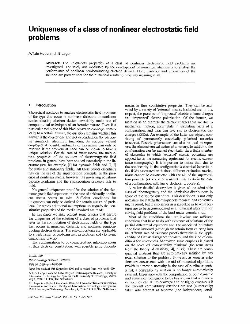
M,,(T) : @(T j + ~ ' " ~ ( 7 ) (101 is defined for any Y € D,, n = 1, ..., N, while in D- we assume that pd = 0. This operator is a scalar operator. The mapping M, is injective, in many cases of practical interest bijective. A physical model for M, is provided by the quantum-statistical theory of semiconductors. In the relevant expressions for the local equilibrium number densi- ties of the (negatively charged) electrons and (positively charged) holes, the quantum mechanical Fermi potential is, by an argument of an energetic nature, equated to the local value of the electiic potential of the energising electric field. This procedure is justified by experimental data. Details of the analysis are given in, for example, [9] (Section 7.2) or [IO]. Figs. 1 and 2 show the relevant functional relationship for holes and electrons, respectively. Note that, in semicon- ducting devices, one particular electrode always setlies as the reference electrode. This electrode is chosen to be the one that ensures the desired electronic operation of the device. In the interior of the semiconducting material, the pertaining Fermi levels then adjust themselves to the elec- tronic potential distribution generated by this operational choice.

2.8 Compatibility relations Eqn. 1 entails the compatibility relation

l sn x E dA = 0 (11)

for any piecewise smooth, closed surface S with unit vector. n = n(u) along its outward normal. Eqn. I I follows from eqn. I by integrating n x V@(r) over S and dividing S arbi- trarily into two parts S' and S", both of which are delm- ited by the same, piecewise smooth, closed curve. Subsequent application of Stokes' circulation theorem to S' and S" shows that the two partial surface integrals cancel each other.

Eqn. 2 entails the compatibility relation

l c 2 n , D dA = L P d V (121

for any hounded domain S with piecewise smooth bound- a y surface a S and unit vector n = n(r) along the outward normal. Eqn. 12 follows from eqn. 2 by the application of Gauss' divergence theorem.

As elucidated in the introduction, the compatibility rela- tions are automatically satisfied by any exact solution to the partial differential eqns. I and 2. In numerical (or other nonexact) procedures they play, however, a role of impor- tance on their own.

2.9 Field properties in exterior domain Finally, the field properties in the exterior domain D" have to be specified. Here, two possibilities arise: (i) the case where proper electrical shielding or dielectric packaging of a device prevents the leakage of the field into its exterior, in which case the exterior field is negligibly small (see Figs. 3 and 4)

4 1 electric potential -

It is assumed that M#) and M,(Y) are continuous in Y in the interior of each Dn, n = 1, ..., N , and approach finite limiting values at JD,,, n = 1, ..., N, while End(r) = EO-' D(r) and pd( r ) = 0 for Y E 27". Across interfaces between adja- cent subdomdins of D, MF and M, may show a jump dis- continuity.

1E.E Prac.-Sci. Meas. Teclmol.. Vol. 146, No. 4, h d i s 1999

Fig. 4

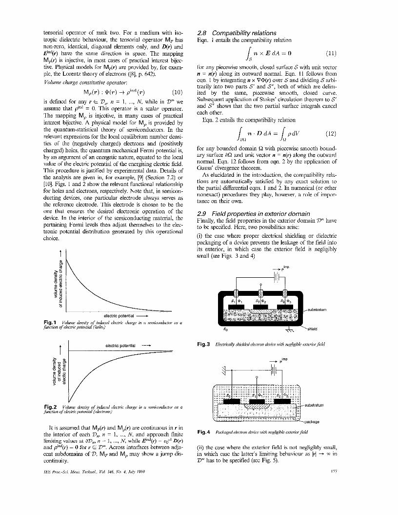
(ii) the case where the exterior field is not negligibly small, in which case the latter's limiting behaviour as 11.1 - in D" has to be specified (see Fig. 5).

Po%iekaged electron device with negiigiL.b exterior field

I77

volume distribution Of impressed

electric charge /

Fig. 5 Packoged e/ecrron device wilh with non-neg/igih/e e,uwiovfie/d

Configurations with negligible exterior f e l d The analysis of configurations with negligible exterior field is covered by prescribing explicit boundary conditions on dD. Let aD' be the part of dD that takes care of the electrical shielding of the device and let dD" he the part of dD that takes care of its dielectric packaging. Then, the nonleakage of the field into 57" is mathematically covered by the boundary condi- tions

and @(r) = 0 for r E dD'

n(r) . D ( r ) = 0 for r E ?XI''

(13)

(14) where n is the unit vector along the outward normal to dD. Configurations with non-negligible exteriorfeld If the previ- ous case does not apply, the behaviour of the field as Ir1 - m in D" has to he prescribed. As is proven in the Appendix (Section 7), the weakest a priori sufficient condition in this respect is @(r) = o(1) as 171 i 00,

uniformly in all directions in DOo (15) which involves the Landau symbol o(l), ([SI, p. 1020), meaning that l@(v)l - 0 as IrI + m. Because of the special structure of the field in the (vacuum) domain D", entailed by the equations

-VQ = E i n d (16)

V . D = O (17)

= (18)

and

where use was made of the fact that (cf. Eqn. 3) P P = 0 and p = 0 in the (vacuum) domain D", the condition in eqn. 15 entails the properties (see the Appendix)

@"d

a(r) = o(lri-') as I T I + 00, uniformly in all directions in D"" (19)

and

D(T) = O ( I T I - ~ ) as lrl + 00, uniformly in all directions in 2)"" (20)

which involves the Landau order symbol 0, ([g], p. 1019).

3 Uniqueness theorem

For the field problem formulated in Section 2, the follow- ing uniqueness theorem will be proven. Theorem I : For given values of the volume source quanti- ties P'"P(v) and p"p(r) and given values V,, m = I , ,,., M , of the electric potential Q, at the electrodes S,, m = 1, ._., M (together with @ = 0 at the reference electrode So), there exists at most one electrostatic field with field quantities

178

{@, D, pd, End} in U L l Dn (for the case of negligible exterior field) or { U z l Dn} U 2)" (for the case of non-neg- ligible exterior field) provided that the constitutive operator M, entails at each point r E U:, 4, the monotonicity relation

[D2(r) -D1(r)] ' [@d(.) - E ' l d ( T j ] > 0

for any { D z ( T ) , E F d ( T ) } # {DI(T),@'~(P)}

(21) and the constitutive operator M, entails at each point Y E Ug1 D,, where p d ( r ) # 0 the monotonicity relation

[@z(r) - @I(.)] [pFd(r) - pfd(r)] < 0

for any {%(T) ,p? ' ( r ) } # {%(T),P?~(T)} (22)

Prooj The proof starts in the standard manner by assum- ing that, for { U ~ , D n } U D" and corresponding to the same set of prescribed excitation quantities, two non-identi- cal fields {@l(vJ. Dl(rJ, plind(rJ, Elind(r)} and {Qz(~), &(VI, prind(r), E2"d(r)} exist. Then, by subtracting the relevant eqns. 1 and 2 for the two fields, we obtain

(23)

(24)

-V(Q2 - a1) = ETd ~ Ei"d 1

and

V . (D2 ~ 01 ) = pyd - ppd Now, consider the expression that results on multiplying eqn. 23 by Dz - Dl and eqn. 24 by Qz - Qi and subtract- ing the results. This yields

-v . [(@z ~ % ) ( 0 2 - Di)]

= ( 0 2 ~ Dl) . (EFd ~ E p d )

~ (@z - @I J (ofd ~ pYd) (25) For the difference field, the interface boundary conditions

(26) and

Y (Dl - 0 2 ) = continuous across interfaces (27) hold, while on the electrodes (including the reference one) we have

@ 2 - @ 1 = 0 o n S , , m = O , ..., M (28) The further proof runs differently for the two cases of neg- ligible and non-negligible exterior fields. Configurations with negligible exterior field For configura- tions with negligible exterior field, the boundary conditions

and

- Q1 = continuous across interfaces

% ( r ) - a 1 ( r ) = 0 for T E 8D' (29)

v . [0l(r) - D ~ ( T ) ] = 0 for T E D" (30) apply (cf. eqns. 13 and 14). Then, integrating eqn. 25 over D,,, n = I , ..., N , applying Gauss' divcrgence theorem, add- ing the results and using the interface boundaly conditions, eqns. 26 and 27, the explicit boundaly conditions eqn. 28 on the electrodes and eqns. 29 and 30 on the boundary surface dD, it follows that

- (a2 - "1) (gd ~ p;"'),] dV = 0 (31)

IEE Proc.-Sci. Meus Technol.. Vol. 146. No. 4, July 1999

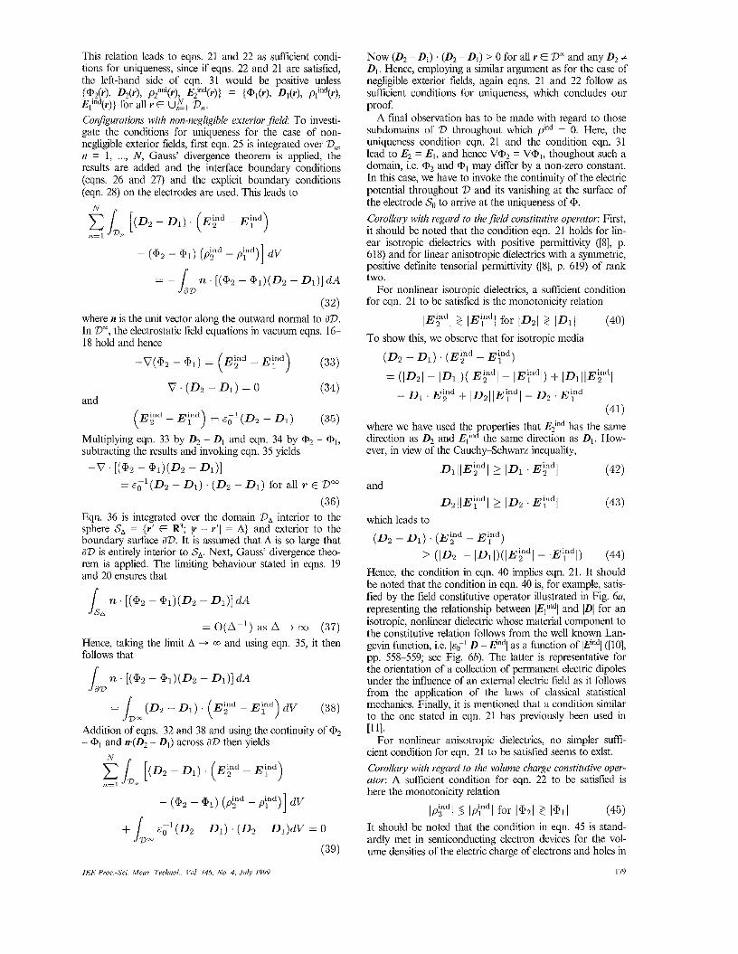
This relation leads to eqns. 21 and 22 as sufticient condi- tions for uniqueness, since if eqns. 22 and 21 are satisfied, the left-hand side of eqn. 31 would be positive unless i @ 2 ( 4 Dz(J9, P ; " d W , EPd(J9) = i@l(J% Dl(4 Pl'"d(U)> Elind(r)) for all I E U,$:, D,?. Confgurutions with non-negligible exterior field: To investi- gate the conditions for uniqueness for the case of non- negligible exterior fields, first eqn. 25 is integrated over D,, n = 1 , ..., N , Gauss' divergence theorem is applied, the results are added and the interface boundary conditions (eqns. 26 and 27) and the explicit boundaty conditions (eqn. 28) on the electrodes are used. This leads to

- ( @ p a - @ I ) (pkd - p;"")] dV

n . [ ( @ a - @ i ) ( D 2 - DI)] d A = - L

(32) where n is the unit vector along the outward normal to aD. In D=, the electrostatic field equations in vacuum eqns. 16- 18 hold and hence

-V(@,, - = (EYd - EYd ) (33)

(EV - E;"") = E O ' ( D * - D l )

v . (D2 - 0 1 ) = 0 (34)

( 3 5 )

and

Multiplying eqn. 33 by D2 - D, and eqn. 34 by a2 - a,, subtracting the results and invoking eqn. 35 yields

-v ' [(a, - Q 1 ) ( 0 2 - Dl)] -1

= E ~ (D2 - 0 1 ) . ( 0 2 - 0 1 ) for all r E Dm (36)

Eqn. 36 is integrated over the domain DA interior to the sphere SA = {r' t R3; )r - r'1 = A) and exterior to the boundary surface dD. It is assumed that A is so large that dD is entirely interior to SA. Next, Gauss' divergence theo- rem is applied. "be limiting behaviour stated in eqns. 19 and 20 ensures that

= 0(4-') as 4 i CXI (37) Hence, taking the limit A + m and using eqn. 35, it then fOllOWS that

Addition of eqns. 32 and 38 and using the continuity of Q2 - a, and m(D, - 0,) across dD then yields

- (aa - ( p y ' -$",I dV

(39)

Now (D2 - D J . (Dz - D l ) > 0 for all I' t D" and any D2 #

DI. Hence, employing a similar argument as for the case of negligible exterior fields, again eqns. 21 and 22 follow as sufficient conditions for uniqueness, which concludes our proof.

A final observation has to be made with regard to those subdomains of 2, throughout which pd = 0. Here, the uniqueness condition eqn. 21 and the condition eqn. 31 lead to E2 = E l , and hence VB2 = VB,,, thoughout such a domain, i.e. Q2 and @, may differ by a non-zero constant. In this case, we have to invoke the continuity of the electric potential throughout D and its vanishing at the surface of the electrode So to arrive at the uniqueness of 0. Corolhuy with regurd to thefield constitutive operuto,.: First, it should be noted that the condition eqn. 21 holds for lin- ear isotropic dielectrics with positive permittivity ([SI, p. 618) and for linear anisotropic dielectrics with a symmetric, positive definite tensorial permittivity ([8], p. 619) of rank two.

For nonlinear isotropic dielectrics, a sufficient condition for eqn. 21 to be satisfied is the monotonicity relation

lEFil 2 IE;""l for ID?/ 2 ID11 (40) To show this, we observe that for isotropic media

(Dl - 01) (EPd - EYd) = (ID21 - 1D11)(1Ep - IEyy) + ID1lIEL""I

- D ~ . E F ~ + p 2 1 1 ~ p d l - D ~ . E F ~ (41)

where wc have used the properties that Epd has the same direction as D2 and Ellnd the same direction as D,. How- ever, in view of the Cauchy-Schwaiz inequality,

IDIIIEYdl 2 IDI.E,"dl (42)

1D211E;"dl 2 ID2 -E""/ (43)

and

which leads to

( 0 2 - D1) . ( E y - E " d )

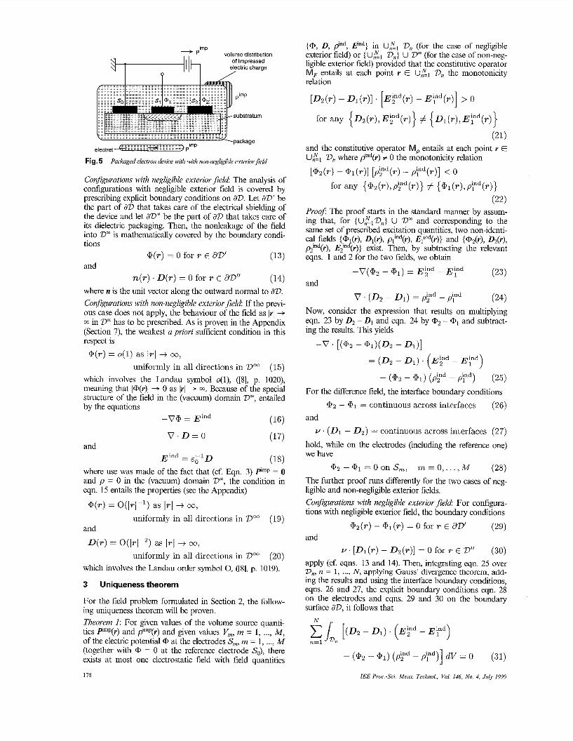
2 (ID21 - IDII)(IEtdl - IE3) (44) Hence, the condition in eqn. 40 implies eqn. 21. It should be noted that the condition in eqn. 40 is, for example, satis- fied by the field constitutive operator illustrated in Fig. 6u, representing the relationship between IElind/ and ID1 for an isotropic, nonlinear dielectric whose material component to the constitutive relation follows from the well known Lan- gevin function, i.e. D - Endl as a function of lEnd1 ([IO], pp. 558-559; see Fig. 6b). The latter is representative for the orientation of a collection of permanent electric dipoles under the influence of an external electric field as it follows from the application of the laws of classical statistical mechanics Finally, it is mentioned that a condition similar to the one stated in eqn. 21 has previously been used in

For nonlinear anisotropic dielectrics, no simpler suft- cient condition for eqn. 21 to be satisfied seems to exlst. Corollury with regard to the volunie charge constitutive oper- utor: A sufficient condition for eqn. 22 to be satisfied is here the monotonicity relation

v11.

IpFdl 4 Ipyl I for /$,I 2 1911 (45) It should be noted that the condition in eqn. 45 is stand- ardly met in semiconducting electron devices for the vol- ume densities of the electric charge of electrons and holes in

119

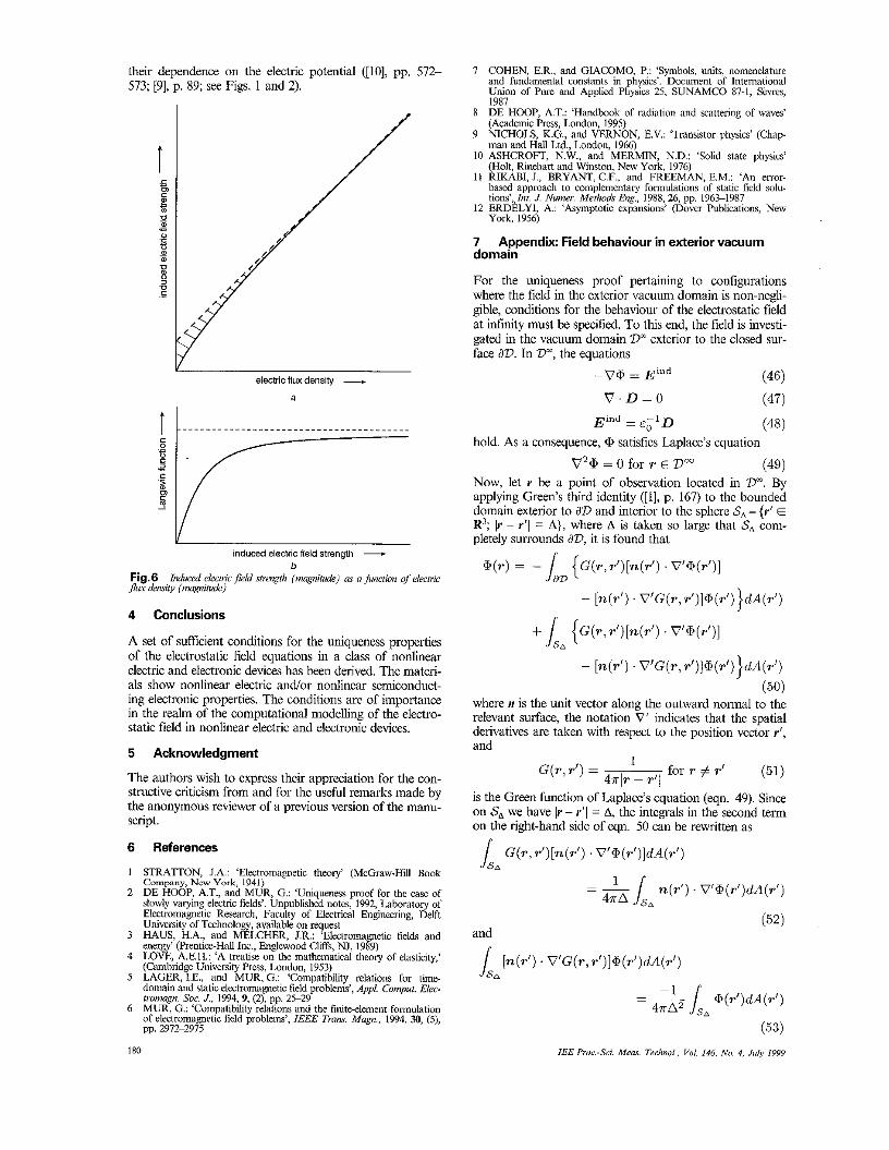
their dependence on the electric potential ([IO], pp. 572- 573; [9], p. 89; see Figs. 1 and 2).

7 COHEN, E.R., and GIACOMO, P.: ‘Symbols, units, nomenclature and fundamental constants m physics’. Document of International Union of Pure and Applied Physics 25, SUNAMCO 87-1, S h e s , 19C7

electricfluxdensin/ - a

induced electric field strength - b

Fig.6 Ju demity (magnitude)

Idreed eleclric fzld mmgth (magzit&) ap n/iiction ofrlecnic

4 Conclusions

A set of sufficient conditions for the uniqueness properties of the electrostatic field equations in a class of nonlinear electric and electronic devices has been derived. The materi- als show nonlinear electric and/or nonlinear semiconduct- ing electronic properties. The conditions are of importance in the realm of the computational modelling of the electro- static field in nonlinear electric and electronic devices.

5 Acknowledgment

The authors wish to express their appreciation for the con- structive criticism from and for the useful remarks made by the anonymous reviewer of a previous version of the manu- script.

6 References

1 STRATTON, J.A.: ‘Electromagnetic theory’ (McGraw-Hill Book Company, New York, 1941)

2 DE HOOP, A.T., and MUR, G.: ‘Uniqueness proof for the case of slowly varying electric fields’. Unpublished notes, 1992. Laboratom of ElecComdgne%c Research, Facdty of Electrical En&eering, Delft University of Technology, available on request

3 HAUS, H.A., and MELCHER, J.R.: ‘Electromagnetic fields and energy’ (F’rentice-Hall Inc., Englewaod Cllffs, NJ, 1989)

4 LOVE, A.E.H.: ‘A treatise on the mathematical theory of elasticity,’ (Cambridge University Press, London, 1953).

5 LAGER, LE., and MUR, 0.:. ‘Compatibility relations for rim* domam and static electromagnetic field problems’, Appl. Compui. Elec- tromugn. Soc. J., 1994, 9, (2), pp. 25-29 MUR, G.: ‘Compatibility relations and the finitedement formulation of electromagnetic field problem’, IEEE Trans. Map. , 1994, 30, (5j, pp. 2972-2975

6

. I~,

8 DE HOOP, A.T.: ‘Handbook of radiation and scattering of waves’ (Academic Press, London, 1995)

9 NICHOLS, K.G., and VERNON, E.V.: ‘Transistor physics’ (Chap- man and Hall Ltd., London, 1966)

10 ASHCROR, N.W., and MERMIN, N.D.: ‘Solid state physics’ (Halt, Rinehart and Winston, New York, 1976)

I I RIKABI, J., BRYANT, C.F., and FREEMAN, E.M.: ‘An error- based approach to complementary formulations of static field sol”. tions’,,lnt. J. Nume?. M e t l d r Eng, 1988, 26, pp. 196S1987

12 ERDELYI, A.: ‘Asymptotic expansions’ (Dover Publications, New York, 1956)

7 Appendix: Field behaviour in exterior vacuum domain

For the uniqueness proof pertaining to configurations where the field in the exterior vacuum domain is non-negl- gible, conditions for the behaviour of the electrostatic field a t infinity must be specified. To this end, the field is investi- gated in the vacuum domain ’D- exterior to the closed s u - face dD. In ’D-, the equations

(46)

(47)

=&,ID (48)

(49)

-VQ, = E ‘ ” d

V . D = O E i n d

hold. As a consequence, satisfies Laplace’s equation

V 2 0 = O for T ED” Now, let Y be a point of observation located in Dm. By applying Green’s third identity ([I], p. 167) to the bounded domain exterior to d’D and interior to the sphere SA = {v ’ E R’; Iv ~ Y ’ I = A}, where A is taken so large that SA com- pletely surrounds 827, it is found that

* ( T ) = - L, {G(T,T’)[Tz(T’) V’@(T’)]

- [n(r’) V’G(~,r’)]O(r’))dA(rl)

- [n(r’) . V’G(~,r’) lO(r’))dA(r’)

where n is the unit vector along the outward normal to the relevant surface, the notation 0’ indicates that the spatial derivatives are taken with respect to the position vector Y’, and

(50)

1 4 ~ 1 ~ - T ’ /

G(T ,T ’ ) = for r # T’ (51)

is the Green function of Laplace’s equation (eqn. 49). Since on SA we have I Y - v’l = A, the integrals in the second term on the right-hand side of eqn. 50 can be rewritten as

G(T, T ’ ) [ ~ ( T ’ ) V’a(~‘)]dA(r’) LA (52)

and

[n(~’ ) . V’G(T, d)]* (~ ’ )dA(r ’ ) x ( 5 3 )

IEE Proe.-Sel. Meas. Tednol.. Vol. 146, No. 4, July I999 180

However, and r

4alrI3 V’G(r,r’) = -[l + O ( ~ T - ’ ) ] as / T I + 00

for E aD (60) it follows that

a(.) = O(lri-’) as 171 + 00,

uniformly in all directions in Dm (61) which is consistent with eqn. 56.

To obtain the asymptotic representation as I Y ~ - m for D in the domain exterior to a’D, we observe that in this region

and, hence, from eqn. 58 it follows that D = -QV@ (62)

which follows on applying Gauss’ integral theorem to the domain DA and using eqn. 49. Combining this with eqn. 52, it follows that

G ( ~ , T ’ ) [ ~ ( T ’ ) . V ’ @ ( r ’ ) l d A ( ~ ’ ) = O(A-’)

as A i 00 (55)

since the integral on the right-hand side of eqn. 54 is bounded. Next, imposing the condition

a(.) = o(1) as 171 + 00,

uniformly in all directions in D“ (56) we have from eqn. 53

l[n(~’).V’G(r,~’)]@(~’)dil(r~) = o(1) as A i cc S A

(57 ) Hence, taking the limit A + m, it follows from eqn. 50 that, subject to the condition eqn. 56, the electric potential admits, in the entire domain exterior to KD, the surface source representation

@(r) = - k,, { G ( ~ , r ’ ) [ n ( d ) . V’@(T’)]

~ [n(r’) B’G(T,~ ’ ) ]@(T’ ) }~A(~‘ ) for T E D” (58)

Using in this representation the asymptotic expansions

G(r,r’) = -[l + O(lrl-’)] as 171 i 00 1

4+1 for T I E aD (59)

-[n(r’) . V’G(r,r’)]@(r’)}dA(?-’)

for r E DW (63) Using in this representation the asymptotic expansions

r 4?rlrI3

VG(r,r’) = -- [I + O(lrl-’)] as I T I + 00 for T’ E dD (64)

and V [n(r’) . V’G(r, d)]

as I T / i 00 for 7’ E d D (65) it follows that

D(r) = O ( ~ T - ~ ) as 171 i 00, uniformly in all directions in D- (66)

Eqns. 61 and 66 are used in the main text. Note that eqn. 66 is compatible with a differentiation of eqn. 61, but since termwise differentiation of an asymptotic expansion is in general not permitted ([12], p. 17), eqn. 66 had to be derived independently.

IEB 1’roc:Sci. iMeiis Technoi.. Voi. 146, No. 4, July 1999 181