Unintended Consequences of LOLR Facilities: The Case of Illiquid Leverage

Viral V. Acharya New York University’s Leonard N. Stern School of Business

Bruce Tuckman

New York University’s Leonard N. Stern School of Business

Paper presented at the 14th Jacques Polak Annual Research Conference Hosted by the International Monetary Fund Washington, DC─November 7–8, 2013 The views expressed in this paper are those of the author(s) only, and the presence

of them, or of links to them, on the IMF website does not imply that the IMF, its Executive Board, or its management endorses or shares the views expressed in the paper.

1144TTHH JJAACCQQUUEESS PPOOLLAAKK AANNNNUUAALL RREESSEEAARRCCHH CCOONNFFEERREENNCCEE NNOOVVEEMMBBEERR 77––88,, 22001133

Unintended Consequences of LOLR Facilities: The

Case of Illiquid Leverage

Viral V. Acharya and Bruce Tuckman∗

October 23rd, 2013

Abstract

While the direct effect of lender-of-last-resort (LOLR) facilities is to forestall thedefault of financial firms that lose funding liquidity, an indirect effect is to allow thesefirms to minimize deleveraging sales of illiquid assets. This unintended consequence ofLOLR facilities manifests itself as excess illiquid leverage in the financial sector, canmake future liquidity shortfalls more likely, and can lead to an increase in default risks.Furthermore, this increase in default risk can occur despite the fact that the combinationof LOLR facilities and reduced asset sales raises the prices of illiquid assets.

The behavior of U.S. broker-dealers during the crisis of 2007-2009 is consistent withthe unintended consequence just described. In particular, given the Federal Reserve’sLOLR facilities, broker-dealers could afford to try to wait out the crisis. While theydid reduce traditional measures of leverage to varying degrees, they failed to reducesufficiently their illiquid leverage, which contributed to their failures or near failures.

Several mechanisms to address this unintended consequence of LOLR facilities areproposed: condition LOLR access and terms on the financial health of borrowers; condi-tion LOLR access and terms on asset sales and deleveraging; and, especially, instead ofsupporting troubled financial firms, open LOLR facilities to financially sound, potentialbuyers of illiquid assets.

∗Viral V. Acharya is the C. V. Starr Professor of Economics in the Department of Finance at the NYU Stern Schoolof Business, a Research Affiliate of CEPR, and a Research Associate of the NBER. Email: vacharya@stern.nyu.edu.Bruce Tuckman is a Clinical Professor of Finance at the NYU Stern School of Business and a Senior Fellow at theCenter for Financial Stability. Email: btuckman@stern.nyu.edu. This paper was prepared for the IMF EconomicReview Conference in Honor of Stanley Fischer. We are grateful to Pierre-Olivier Gourinchas and Ayhan Kose(editors) as well as three anonymous referees for helpful comments. We thank Katherine Waldock for outstandingresearch assistance. All errors remain our own.

1 Introduction

Since 2007, central banks worldwide have offered lender-of-last-resort (LOLR) facilities to private

financial institutions in unprecedented scope and scale. These facilities provide funding against

relatively illiquid assets in times of market stress so as to prevent downward spirals in which

balance sheet weaknesses beget asset fire sales, which beget further balance sheet weaknesses, etc.,

until the financial sectors ruin devastates the real economy.

LOLR facilities are hardly a panacea, however. The ex-ante moral hazard of providing such

facilities in a crisis is well and widely recognized: financial institutions, knowing that authorities

will offer liquidity in a crisis, take too much liquidity risk from a societal perspective. In addition,

despite the ex-post societal benefits of LOLR facilities, the sense in which these facilities bail out

financial institutions generates considerable political fallout.

This subject of this paper is a less recognized moral hazard of LOLR facilities, which occurs

when these facilities are in operation. Consider the following exchange at Merrill Lynch’s earnings

call from the second quarter of 2008. Meredith Whitney, a well-known analyst at Oppenheimer,

asked John Thain, Chairman and CEO of Merrill Lynch, whether the firm could put its balance

sheet problems behind it by “hitting whatever cash bid... is out there” for its troubled assets. Mr.

Thain responded as follows:

We have not simply liquidated stuff at any price we could get. At some point some

of the return profiles that people want... you would not want us to sell the assets. We

will continue to sell assets but in a way that makes sense from generating returns to

our shareholders.1

Out of context, this response seems perfectly reasonable: the CEO of a financial institution

is promising to conduct asset sales so as to maximize shareholder returns. In context, however,

Mr. Thain’s statement is quite remarkable. Following the collapse of Bear Stearns in mid-March

2008, the Federal Reserve established unprecedented LOLR liquidity facilities, namely the Term

Securities Lending Facility (TSLF) and the Primary Dealer Credit Facility (PDCF), to ease the

precarious funding conditions that were perceived to threaten the very survival of broker-dealers.

1Merrill Lynch, Q2 Earnings Call, July 17, 2008

1

It would not be unreasonable to expect broker-dealers to use the respite provided by these facilities

to sell troubled assets gradually, i.e., to strengthen their balance sheets without dumping assets

in an individually and systemically harmful manner. Instead, while the Federal Reserve, and by

extension the U.S. taxpayer, stood ready to fund assets and assume whatever risks that entailed,

the CEO of a beneficiary of these LOLR facilities proclaimed that asset sales would be conducted

so as to generate returns for shareholders. Worse yet, Merrill Lynch’s delay in deleveraging its

balance sheet, made possible at least in part by LOLR facilities, was a factor contributing to its

demise as an independent firm in September 2008, a mere two months after Mr. Thain’s remarks.

The case of Merrill Lynch in July 2008 is only a single instance of a much wider phenomenon.

Whether considering the Federal Reserve’s set of LOLR programs in the U.S. during the ’07-’09

financial crisis, including traditional discount window lending, the Bank of Japan’s Funds Supply-

ing Operation in ’09-’10, or the European Central Bank’s (ECB’s) recent Long-Term Refinancing

Operations (LTRO), there is a concern that private financial institutions take advantage of central

bank funding programs by dragging their feet on deleveraging. With this motivation, this paper

argues, both theoretically and through a case study, that LOLR facilities as currently designed

can have the unintended consequence of reducing the extent to which financial firms delever and,

therefore, can actually increase these firms’ risks of default.

To establish its theoretical results, this paper constructs a model designed to capture the

plight of many banks and investment banks during the most recent crisis. In particular, a repre-

sentative bank has borrowed short-term to fund the purchase of long-term and relatively illiquid

assets. Then, due to market stress, these assets sell for less than their fundamental values and

have become difficult to finance.2 The bank, consequently, needs to delever, i.e., to sell some of its

assets, despite their being undervalued, so that the firm has enough funds on hand to redeem any

maturing debt that cannot be rolled over.

The central bank steps into this setting by offering to fund the illiquid asset at better terms

than those offered by private funding markets. The direct effect of such an LOLR facility, the

2Broker-dealers normally rely on private markets to finance their positions, but these markets became severelyimpaired in early 2008. Lenders of funds through repurchase agreements became increasingly cautious, worryingboth about the liquidation value of collateral and about the credit risk of counterparties. These lenders reacted byincreasing haircuts reducing the cash they were willing to lend against a given amount of collateral and by refusingto lend at all against certain types of collateral. See, for example, Copeland, Martin and Walker (2011), Gorton andMetrick (2012), and Krishnamurthy, Nagel, and Orlov (2012).

2

“liquidity insurance effect,” is to forestall the default of a bank in all but the worst stress condi-

tions. The indirect effect, however, the “moral hazard effect,” is to give the bank leeway to reduce

deleveraging sales of illiquid assets. In the simplest version of the model, where the price of the

illiquid asset is exogenous, the moral hazard effect not only exists, but dominates the liquidity in-

surance effect so that the LOLR facility actually increases the risk of a bank default. Furthermore,

the moral hazard effect can be particulary powerful for the weakest or most highly-levered banks.

The paper then considers a version of the model to account for the fact that the illiquid asset

price is actually determined endogenously, which has implications for any equilibrium conclusions

about the effects of LOLR facilities. More specifically, the model introduces a representative buyer

of the asset as a stand in for those less leveraged banks and investment banks, hedge funds, pension

funds, insurance companies, asset managers, etc., who are able to purchase distressed assets oppor-

tunistically in a crisis. The bank’s supply curve, or willingness to sell the illiquid asset, together

with the buyer’s demand curve, or willingness to buy the illiquid asset, combine to determine the

asset’s equilibrium price. Analytic results are more elusive in this model, but, restricting equilibria

to those in which LOLR facilities increase the price of the illiquid asset, numerical analysis shows

that the qualitative results of the simpler model obtain. In particular, the moral hazard effect

still exists and, for certain ranges of LOLR funding terms, the LOLR facility increases the bank’s

probability of default.

The version of the model with an endogenously-determined asset price generates a further

result that has particular relevance for public policy. Giving the buyer access to the LOLR facility,

instead of the troubled bank, results in an equilibrium with a higher illiquid asset price, a higher

degree of bank deleveraging, and a lower probability of bank default. In other words, a buyer-access

LOLR facility may overcome the moral hazard that is the subject of this paper.

The case study section of the paper shows that the behavior of U.S. broker-dealers during the

crisis of 2007-2009 is consistent with the model and its results. The section starts with a primer

on broker-dealer balance sheets and introduces “illiquid inventory leverage,” a new measure of a

financial firm’s risk that is more consistent with market concerns during the crisis than are the

more traditional measures of leverage. The paper then documents the deleveraging behavior of

broker-dealers after the establishment of the TSLF and PDCF in mid-March 2008. The weakest

two broker-dealers, namely Lehman Brothers and Merrill Lynch, did reduce broader measures

3

of leverage, but did little to reduce their most important exposures, i.e., their risks to illiquid

assets, and failed in September 2008. The strongest two broker-dealers, namely Morgan Stanley

and Goldman Sachs, did reduce illiquid leverage substantially in response to the the fall of Bear

Stearns, but then took a break from deleveraging in the third quarter of that year. In the market

turmoil following the bankruptcy of Lehman Brothers, however, Morgan Stanley and Goldman

Sachs resumed their reduction of illiquid asset inventory, but market conditions at that point

limited what they could accomplish.

The facts of broker-dealer deleveraging are consistent with the model of the paper: during a

crisis, with the security of LOLR facilities in place, broker-dealers delevered relatively slowly, and

the weaker among them delevered most slowly. Only anecdotal evidence, however, can connect these

facts with the motives driving broker-dealer behavior. To that end, this paper reviews statements of

broker-dealer management during earnings calls, like the Merrill Lynch call recounted earlier. This

body of evidence indicates quite clearly that management understood the significance of existing

LOLR facilities, but set deleveraging strategies to maximize their firms’ private interests.

The paper concludes with two sets of policy recommendations motivated by the theoretical

and empirical results just described. The first set of recommendations is to mitigate the moral

hazard of reduced deleveraging directly, i.e., by conditioning access to LOLR facilities on some

degree of leverage reduction or asset sales. The extent of the conditioning would be calibrated,

of course, so as not to sacrifice unduly the systemic benefits of the LOLR facilities. Importantly,

to this end, the conditioning can be implemented so as to exlclude funding of customer positions.

The second set of recommendations is to encourage institutions with relatively clean balance sheets

to use the LOLR facilities to purchase illiquid assets. This policy could temporarily support the

price of such assets while facilitating, rather than slowing, the deleveraging of troubled financial

institutions.

The outline of the paper is as follows. Section 2 reviews the related literature. Section 3

presents and analyzes the model with an exogenously-determined illiquid asset price while Section

4 extends the model to an endogenously-determined price. Section 5 presents the case study of

broker-dealer deleveraging from ’07 to ’09. Section 6 presents our policy recommendations and

Section 7 concludes.

4

2 Literature Review

Recent theoretical literature recognizes the nexus of bank liquidity, solvency, and LOLR policies.

Rochet and Vives (2004) and Diamond and Rajan (2005) stress that it is generally difficult to

distinguish between an illiquid and an insolvent institution, which implies that a central bank can

easily find itself lending to an insolvent institution. Their results suggest that the much celebrated

prescription of Bagehot (1873) for LOLR policies might be right after all. He proposed that the

central bank, in times of panic, freely advance reserves to any private bank able to offer “what in

ordinary times is reckoned a good security” as collateral, but at a penalty rate, so as to discourage

applications from banks not really in need of funds. While Bagehot was concerned primarily with

the practical goal of conserving limited reserves, this literature provides a new rationale for such

intervention.3

On the theoretical front, this paper is related both to Rochet and Vives (2004) and Diamond

and Rajan (2005), but is more specifically focused on understanding how LOLR facilities affect

the deleveraging decisions of financial institutions and the market prices of illiquid assets. More

specifically, when does the moral hazard effect of LOLR facilities, which reduces deleveraging at

eligible firms, increase their likelihood of default, despite the fact that LOLR increases asset prices?

On the empirical front, evidence has accumulated on how the provision of central bank

liquidity relaxes institutions’ funding constraints, and thereby supports the prices of illiquid assets.

See Fleming (2012), for example, for a review of studies documenting that the Federal Reserve’s

suite of LOLR policies during the recent financial crisis lowered inter-bank borrowing spreads and

raised the prices of asset-backed and mortgage-backed securities. Empirical work on the ex-ante

incentives of firms participating in LOLR facilities, however, like the case study in this paper, is a

relatively new line of investigation.

Acharya et al. (2011) find that the weaker broker-dealers borrowed at the Federal Reserve’s

TSLF and PDCF, even after controlling for the size of their illiquid inventory. Acharya and Steffen

(2012) document that under-capitalized banks in the peripheral countries, especially Spain and

3See Fischer (1999) for an excellent survey of LOLR policy prescriptions and the literature that evolved theseprescriptions. Although Fischer’s focus is on the role that can be played by the International Monetary Fund (IMF)as the international LOLR when sovereign or banking crises need to be contained from spreading across borders, healso succinctly presents the argument underlying the moral hazard induced by LOLR, including domestic LOLR. Herecognizes that, while moral hazard needs to be contained, it is unlikely to be eliminated entirely through the designof LOLR facilities.

5

Italy, used the ECB’s LTRO to increase their exposures to relatively risky domestic bonds, thus

tightening the feedback loop between banks and sovereigns in the periphery.4 Drechsler et al.

(2013), using data on collateral tendered to the ECB, find that that liquidity facility was used by

some of the riskier firms in the periphery to hold on to their illiquid and risky positions, which

included not only sovereign credit but also mortgage-related investments.

Implicit in much of this empirical work is the underlying fact that the terms (e.g., tenor,

interest rate, haircut, and collateral eligibility) of the LOLR operations of the Federal Reserve,

the ECB, and the Bank of England did not, for the most part, depend on the health of eligible

banks and broker-dealers.5 One rationale for this kind of extensive and unconditional support from

central banks is that banking sector recapitalizations, which can easily require public funds, may

not be feasible due to political economy constraints, such as myopia, as in Acharya and Rajan

(2013). Growing empirical evidence, including that in this paper, however, clarifies that central

bank support is no panacea as it has the unintended consequence of slowing down the deleveraging

process and potentially increasing the likelihood of future crises.

One policy proposal in this paper to address this unintended consequence is to condition

LOLR support on participant solvency. This proposal is related to Acharya and Backus (2009)

who argued that central bank liquidity provision should be made conditional on adequate solvency

estimates of financial institutions, e.g., maximum leverage ratio or minimum capital adequacy.

Lack of such conditionality can allow weaknesses of these institutions to fester, creating “zombie

banks” and further deepening the crisis.6 A related policy proposal in this paper is to condition

LOLR support on a certain amount of deleveraging or asset sales, which would likely stabilize the

borrower.

Both of these policy proposals are related to the discussion in the international context, along

the lines of Fischer (1999). Emergency support by the International Monetary Fund (IMF), a form

of international LOLR, can allow participating countries to slow structural reforms, which might

4See Acharya, Drechsler and Schnabl (2010, 2012) for theoretical and empirical illustrations of how financial-sectorand sovereign credit risks impact one another.

5In a particularly startling example, Acharya and Steffen (2012) show that the Bank of Cyprus, using ECBfinancing, appears to have quadrupled its holdings of Greek debt 2010-11.

6Caballero, Hoshi and Kashyap (2008), in the context of the Japanese banking crisis of the 1990s, attributes thephenomenon of “zombie banks” lending to “zombie firms,” along with the resulting credit crunch, to the excessiveforbearance of the Bank of Japan. Diamond and Rajan (2011) argue that delaying fire sales in expectation of centralbank or government support can increase the returns to liquidity (i.e., to the capacity for acquiring assets that areeventually sold in fire sales) and lead to an ex-ante freeze in credit markets.

6

make future sovereign crises more likely. This moral hazard justifies both linking lending rates to

measures of solvency and conditioning IMF support on strict and possibly unpopular structural

reforms. Fischer (1999) recognizes that an extreme form of conditioning, e.g., not lending to certain

countries altogether, may lack credibility if they or their banks are too big to fail. In that case

Fischer (1999) recommends that those receiving support be pushed by the IMF toward growth-

friendly reforms with respect to, for example, fiscal prudence, monetary and financial transparency,

securities markets standards, bankruptcy regulations, and entry of foreign banks.

Another proposal in this paper is to provide liquidity not to distressed financial intermediaries,

but to potential buyers of distressed assets. These potential buyers must be financially strong, of

course, so as not merely to shift the insolvency problem from one set of firms to another. He,

Khang and Krishnamurthy (2010), studying the adjustment of balance-sheet assets in the United

States from 2007-2009, find that much of the leverage shifted from segments of the financial sector

without access to LOLR financing (i.e., hedge funds and initially broker-dealers) towards segments

covered by LOLR financing (i.e., commercial banks) or by government support (i.e., Fannie Mae

and Freddie Mac). The proposal in this paper is more nuanced than such an arrangement, calling

for the provision of LOLR financing to any healthy, buyers of assets rather than to a pre-ordained

set of financial firms, such as commercial banks and thrifts, that already happen to have access to

LOLR facilities. Indeed, some firms with such access or with government support (e.g., Washington

Mutual, Citibank, GSEs) were excessively leveraged at the time they received public or central bank

support. Judicious design of LOLR policy can prevent the shift of leverage between firms in a way

that has adverse or uncertain consequences for financial stability. Indeed, the proposal to provide

liquidity to healthy potential buyers of assets can improve the ex-ante incentives of financial firms

to manage risks prudently and to keep capacity to purchase assets opportunistically.7

3 The Model with an Exogenous Illiquid Asset Price

This section presents a model designed to explore how LOLR facilities might affect the deleveraging

policy of a bank and its probability of default. The setting is the collision of a financial crisis and

7A result from Acharya and Yorulmazer (2008) resonates here. In that model, in the case of multiple bank failures,the optimal use of fiscal funds is to transfer liquidity to survivors. This curbs the ex-ante incentives for banks to herdin owning correlated assets so as to induce bailouts in cases of en masse failures.

7

an intermediary engaged in maturity and liquidity transformation. More specifically, a bank owns

a long-term, illiquid asset that has been funded, in part, by short-term debt. A poor economy

has reduced the expected cash flows of the asset, and distressed market conditions have depressed

the asset’s price even further. Under these circumstances, the bank would like to hold on to its

undervalued, illiquid asset, but, should its cash flows turn out to be particularly low, and should the

bank not be able to roll over enough of its short-term debt, the ensuing bankruptcy would wipe out

all of the bank’s equity. The bank will, therefore, choose to sell some of its illiquid asset holdings.

How much it chooses to sell, i.e., the extent to which it chooses to delever, depends crucially on

the extent to which it can fund its illiquid asset holdings as its short-term debt comes due. And

the availability of such funding during a financial crisis often depends on the the existence of an

LOLR facility.

The model yields two main results. First, an LOLR facility reduces a bank’s optimal amount

of deleveraging. Very simply, the ability to draw on LOLR funding when needed makes it less risky

for a bank to hold on to its illiquid assets. Second, LOLR facilities increase a bank’s probability

of default. It is clearly true that, for a given portfolio, the availability of LOLR funding lowers the

bank’s probability of default. But the LOLR facility increases the bank’s holdings of the illiquid

asset, as per the first result, which increases the bank’s probability of default. Despite the two

offsetting effects on the probability of default, in the model of this section the moral hazard effect

of increased risk taking always outweighs the liquidity insurance effect of available funding so as to

increase the bank’s probability of default.

Numerical examples of the model illustrate these two main results, along with the relationship

between initial leverage and the optimal amount of deleveraging. It turns out that, for large enough

initial leverage, a bank chooses optimally not to delever at all. As it becomes difficult to avoid

bankruptcy, even with the LOLR facility, it is best for equity to hold on to the upside potential of

the illiquid asset as long as possible.

3.1 Assumptions and Notation

The model has three dates, which are labeled 0, 1, and 2, and two assets. The liquid asset has a

price that equals 1 on every date, which implies a riskless rate equal to 0. The illiquid asset pays

x1 = x̄1 + u on date 1 and x2 > 0 on date 2, where x̄1 and x2 are constants and u is stochastic

8

with cumulative distribution and density functions of G(·) and g(·), respectively. The stochastic,

date-1 cash flow of the illiquid asset introduces a risk of bankruptcy to banks that are funding the

asset with short-term debt, i.e., with debt that matures on date 1. The positive, date-2 cash flow

of the asset motivates banks to avoid bankruptcy on date 1.

The price of the illiquid asset is given exogenously as p per unit, where p < x̄1 + E[u] + x2

and E(·) is the expectations operator. This condition on price ensures that the illiquid asset is

desirable as a positive expected value investment. The assumption of price exogeneity, by the way,

as mentioned in the introduction, will be relaxed in the next section.

Funding or repurchase markets work in the model as follows. A holder of illiquid assets can

borrow on date 1, on a secured basis, a fraction l < 1 of the date-2 cash flow of those assets.

The amount borrowed must be repaid on date 2. Borrowing and lending are effected through

the liquid asset at an interest rate of zero, as discussed earlier. Without access to an LOLR

facility, the fraction l represents the fraction advanced to a holder of the illiquid asset by private

funding markets. With access to an LOLR facility, the fraction l represents the maximum of the

fraction advanced by private funding markets and the fraction advanced by the LOLR facility.

This interpretation highlights the following phenomenon. When an LOLR facility stands ready to

advance a fraction l to a particular set of counterparties, private funding markets are often willing

to advance that same fraction l to that same set of counterparties. After all, should a lender need

its funds returned, the borrowing counterparty can always turn to the central bank for funds. Put

another way, when l is offered by the LOLR facility and is the highest advance fraction available in

the market, holders of the illiquid asset might nevertheless be borrowing that advance from private

markets.

The bank in the model is endowed on date 0 with eL of the liquid asset, eI of the illiquid

asset, and short-term debt outstanding of B, which must be repaid on date 1. To discharge this

date-1 debt obligation, the bank may borrow at the LOLR advance rate of l, as just described.

The bank is assumed to be solvent in the sense that the market value of its assets exceeds its debt

obligations, i.e., eL + peI > B.

Given its endowment, the nature of the assets, and its access to LOLR funding, the bank,

on date 0, maximizes the value of its equity by selling some quantity α of the illiquid asset for p

per unit (and investing the proceeds in the liquid asset). Note that, since bank equity is worthless

9

if the bank defaults on date 1, the date-0 value of the equity equals the expected value of its net

worth on date-2 conditional on the bank’s ability to discharge its date-1 debt.

Table 1 summarizes the bank’s cash flows for a given α assuming no date-1 default. The

bank starts on date 0 with liquid and illiquid asset endowments of eL and eI , respectively. On

date 0 the bank chooses to sell α of the illiquid asset for pα of the liquid asset. On date 1, the

bank carries over its liquid asset balance from date 0; collects its date-1 illiquid asset cash flow of

(eI − α)x1, which it invests in the liquid asset; borrows (eI − α)lx2 from the LOLR facility in the

form of the liquid asset; and pays off its debt of B from its liquid asset holdings. Finally, on date

2, the bank carries over its date-1 liquid asset balance; collects its date-2 illiquid asset cash flow

of (eI − α)x2, which it converts to liquid assets; and pays off its date-1 LOLR borrowing from its

liquid asset holdings. The value of the bank’s equity, therefore, conditional on no default, is simply

its expected date-2 liquid asset balance.

Note the implicit assumption of this discussion and of Table 1 is that the bank always borrows

the most it can borrow from the LOLR facility on date 1. This is a harmless simplification in the

context of this model. First, there are some realizations of u for which the bank does need to

borrow this maximum amount to avoid bankruptcy. Second, with an effective interest rate of 0,

there is no cost to borrowing more than necessary from the facility on date 1 and repaying the full

amount on date 2.

For a final observation on the model setting, make the sensible assumption that date-1 LOLR

loans are available to the bank only if it does not default on date 1. In that case, the bank never

defaults on its LOLR borrowing: it is advanced only a fraction l < 1 of its deterministic date-2

cash flow. More specifically, the bank is advanced (eI − α)lx2 on date 1, while, ruling out a date-1

default, it collects the greater quantity, (eI − α)x2, with certainty.

3.2 The Bank’s Optimal Deleveraging Policy

The bank’s problem is to choose α on date 0 so as to maximize its expected date-2 net worth

conditional on not defaulting on date 1. Focusing for a moment on the condition for not defaulting,

the bank can meet its debt obligation so long as eL + pα+ (eI − α)(x1) + (eI − α)lx2 ≥ B, where

x1 = x̄1 + u. Furthermore, since the only stochastic component of this condition is u, there is

some realization of u below which the bank defaults and above which the bank does not default.

10

Denoting this default threshold value of u as uB, the condition for no default can be written as

u ≥ uB ≡1

(eI − α)[B − eL − (eI − α)x̄1 − (eI − α)lx2 − pα] (1)

The equity value of the bank, E, that is, its date-2 net worth conditional on not defaulting,

can now be written as

E =

∫ ∞uB

[eL + pα−B + (eI − α)x1 + (eI − α)x2]g(u)du (2)

where the integrand is the date-2 liquid asset holding of the bank conditional on no default, as

given in Table 1. Rewriting this integrand in terms of uB,

E = (eI − α)

∫ ∞uB

[(u− uB) + (1− l)x2]g(u)du (3)

Maximizing E with respect to α gives this first-order condition:

∂E

∂α=

−E(eI − α)

− (eI − α)[1−G(uB) + (1− l)x2g(uB)]

(−∂uB∂α

)= 0 (4)

The partial derivative of uB with respect to α can be calculated directly from the definition

of uB in equation (1),

∂uB∂α

=−eL − eIp+B

(eI − α)2< 0 (5)

where the inequality follows from the bank’s solvency condition given in the previous subsection.

Intuitively, as the bank sell more of the illiquid asset, the default threshold falls, i.e., bigger adverse

shocks are required to trigger a default, which means that the probability of default falls. In any

case, substituting expression (5) into (4) gives the final form of the first order condition:8

8This first order condition does not always obtain, that is, under certain conditions the bank will be at a cornersolution. Furthermore, the transition to a corner solution may not be continuous in l or B. Such corner solutions areinteresting because a jump from a positive, optimal α to 0 represents a shift in strategy from deleveraging to purerisk-shifting.

11

∂E

∂α=

1

(eI − α)

[−E + (eL + eIp−B)(1−G(uB) + (1− l)x2g(uB))

]= 0 (6)

3.3 The Effect of LOLR on Deleveraging and Default Probabilities

This subsection presents two results of the model, namely, that an LOLR facility reduces the ex-

tent to which a bank delevers and increases its probability of default. The proofs are in Appendix A.

PROPOSITION 1: dα∗

dl ≤ 0.

The intuition of Proposition 1 is straightforward. The more a bank can borrow against a

given illiquid asset holding, the lower its probability of default. Alternatively, increasing l makes

illiquid asset holdings more affordable in terms of default risk. Therefore, a bank responds to more

generous funding terms by optimally choosing to delever less. Recalling the discussion of l from

earler in this section, by the way, an increase in l can be interpreted either as an LOLR facility

providing better funding terms than previously available private funding or, more literally, as an

LOLR facility liberalizing its previously existing lending terms.

PROPOSITION 2: Unless α∗ = 0, duBdl > 0

To develop some intution for Proposition 2, express duBdl as the sum of two terms:

duBdl

=∂uB∂l

+∂uB∂α

dα∗

dl(7)

The first term on the right hand side is the liquidity insurance effect. The more a bank can

borrow against the illiquid asset, the lower its default threshold and the lower its probability of

default. It is clear from equation (1), in fact, that ∂uB∂l = −x2 < 0, i.e., the liquidity insurance

effect always decreases bank risk.

The second term on the right hand side of equation (7) is the moral hazard effect. The bank

12

takes account of a change in l in its optimal deleveraging strategy. Knowing that l has increased,

the bank chooses to hold more of the illiquid asset, or, equivalently, chooses a lower α, as shown

in Proposition 1. But this reduced deleveraging increases the default threshold and increases the

probability of default, as shown in (5). Mathematically, since both factors of this second term are

negative, their product is positive. Hence, the moral hazard effect always adds to bank risk.

With the liquidity insurance effect decreasing risk and the moral hazard effect increasing risk,

the real thrust of Proposition 2 is the conclusion that the moral hazard effect dominates so that

LOLR facilities increase bank risk. This result will not be as strong in the next section, where the

illiquid asset price is determined endogenously. For now, however, the paper turns to numerical

examples of the model currently under consideration.

3.4 Numerical Examples and Comparative Statics

In the spirit of the model just presented, the setting of these examples is a bank that, in better

times, borrowed short-term funds to finance the purchase of a long-term, relatively illiquid asset.

The quality of the asset then deteriorated, i.e., its price fell, its expected cash flows fell, the volatility

of its cash flows increased, and the haircut required to fund the asset in private markets increased.

As a result, the bank may very well not be able to raise sufficient funds when it needs to refinance

the asset to pay off outstanding short-term debt. In other words, the bank may very well default

on its short-term debt and, consequently, lose the longer-term cash flows of the asset. The bank

chooses, therefore, to sell some portion of its illiquid asset holdings. Crucial to this decision, of

course, are the terms of any LOLR lending facility through which the bank can raise funds on the

collateral of its remaining asset holdings.

3.4.1 Base Case Parameters

Consider the following base case:

i. A bank is endowed with one unit of the illiquid asset at time 0. This asset pays 1 + u at

time 1 and 1.10 at time 2, where u is normally distributed with a mean µ = 0 and a standard

deviation σ = 0.25.

ii. The bank has short-term debt outstanding, which requires a payment of 1.75 on date 1.

13

iii. Through an LOLR secured-lending facility, the bank may, on date 1, borrow 85% of the date-2

cash flow of the risky asset. This borrowing must be repaid on date 2.

iv. The price of the risky asset is 2.098. This price is exogenous in this setting, but will emerge as

the general equilibrium price in an example later in the paper.

This bank is at significant risk of default. Say that the asset were to experience a one

standard-deviation adverse shock, i.e., u = −0.25, so that its date-1 cash flow were 0.75. Then,

even after raising 0.935 through the LOLR (i.e., 85% of the date-2 cash flow of 1.10), the bank’s

cash balance is only 0.75 + 0.935, or 1.685, which is insufficient to repay the maturing debt of 1.75.

One measure of the riskiness of this bank’s balance sheet is its illiquid inventory leverage. Its only

asset is one unit of the risky asset, which is worth 2.098. The book value of its debt is 1.75, which

gives a book equity of 2.098 − 1.75, or .348. Hence, the bank’s illiquid inventory leverage is 2.0980.348 ,

or a bit over 6.0.

3.4.2 Results

Recognizing that holding the full unit endowment of the illiquid asset is too risky, the bank chooses

to sell α of that asset so as to maximize its equity value. Using the base case parameters, the

optimal α turns out to be 0.60, or, equivalently, the bank chooses to retain only 0.40 of its original

unit position. Furthermore, a holding of this reduced size implies a probability of default on date

1 of 0.2%.

Figures 1 (a) and 1 (b) show how the bank’s optimal α, and probability of default change

with l, the fraction of the date-2 cash flow that can be financed through the LOLR facility. Figure

1 (a) shows that α decreases with l. The more generous the LOLR, the more the bank can raise on

the date-2 cash flow of the illiquid asset, and the less the bank chooses to delever. This is the moral

hazard effect of LOLR facilities. Imagine for a moment that the private market would finance only

50% of the date-2 cash flow. Then, according to Figure 1 (a), the bank would sell about 0.76 of its

illiquid asset holdings. Given the existence of an LOLR facility with l = 85%, however, the bank

optimally sells only 0.60 of its holdings. Note too that as the l rises above 88%, α drops to 0, i.e.,

the bank chooses not to delever at all.

Figure 1 (b) shows that the bank’s probability of default increases with l. At l = 50% the

14

probability of default is about 0.02%, while at l = 85% the probability of default is more than

10 times higher at about 0.22%. For any fixed α, the probability of default decreases with l: the

more the LOLR facility lends against the illiquid asset, the less likely a default. However, because

the bank reduces α as the LOLR facility becomes more generous, the net effect is to increase its

probability of default. In this way, one of the goals of LOLR, namely, to reduce the likelihood of

bank defaults, is fully subverted by the moral hazard effect of reduced deleveraging. Note that

moving to the highest levels of l in Figure 1 (b), like 89%, at which level the bank chooses not to

delever at all, the probability of default rises dramatically to about 18%, which is off the scale of

Figure 1 (b). Any further increase in l will, of course, lower the probability of default since α is

from then on fixed at 0.

Figures 2 (a), 2 (b), and 2 (c) show how the bank’s optimal α and probability of default

change with illiquid inventory leverage, a measure of the risk of a bank’s balance sheet. Leverage

is varied for these figures by varying B, the amount of debt due on date 1. For very low leverage,

when the probability of default is zero, the bank does not need to sell any of its illiquid asset.

For intermediate levels of leverage, the bank chooses α, the extent of deleveraging, to target a

probability of default of approximately 0.22%. Finally, for even higher levels of leverage, the bank

chooses not to delever at all and the probability of default jumps to nearly 50% and higher, which,

as that is off the scale of Figure 2 (b), is shown in Figure 2 (c). At these elevated risk levels,

the relatively small increase in survival probability from deleveraging does not compensate for the

foregone returns on the illiquid asset. This result will be invoked later in the paper to explain, at

least in part, why particular investment banks failed to reduce illiquid inventory leverage in 2008.

4 The Model with an Endogenous Illiquid Asset Price

No discussion of bank deleveraging can be complete without some discussion of the behavior of those

who purchase the illiquid asset that the banks are selling. The most likely purchasers certainly need

to have the balance sheet and risk capacity to purchase distressed assets in a time of crisis, but they

must also be knowledgeable about the asset and operationally and legally prepared to own it. These

likely purchasers could include banks with less-levered balance sheets, other levered money with

spare capital and risk capacity, e.g., hedge funds, and real money, wealth management institutions,

15

pension funds, and insurance companies.

With respect to the results of this paper, the interaction of the buyers of the asset and the

banks will determine how the price of the illiquid asset changes as the terms of an LOLR facility

become more or less generous. How robust are the results of the model of Section 3, in which price

is fixed and exogenous, to a setting in which price is endogenously determined?

This section lays out a model in which the price of the illiquid asset is determined by the

supply from banks and the demand from potential buyers. While it is difficult to draw general

conclusions from this substantially more complicated world, it is not difficult to show numerical

examples in which the results of the previous section obtain, i.e., in which LOLR facilities reduce

bank deleveraging and increase the probability of bank default.

The model of this section allows for the possibility that the buyers have access to an LOLR

facility, either along with the banks or instead of the banks. Numerical results in these cases will

be invoked in the policy discussion of Section 6.

4.1 Assumptions and Notation

The properties of the asset, the rules of the LOLR facility, and the characteristics of the bank are

the same here as in Section 3. Therefore, changing notation by indexing quantities, the bank’s

optimization problem here is identical to that of Section 3, i.e.,

maxαBank

EBank = (eI,Bank − αBank)∫ ∞uBankB

[(u− uBankB ) + (1− lBank)x2]g(u)du (8)

The model notation for the buyer is very much like that for the bank. The buyer has

endowments of the liquid and illiquid assets, it has debt due on date 1, and it has access to the

LOLR facility with the parameter lBuyer. The buyer’s decision variable, however, which is denoted

αBuyer, gives the amount of the illiquid asset bought, rather than sold, on date 0. Table 2 puts

all of this together to illustrate the cash flows of the buyer for a given αBuyer conditional on no

default. This table is, of course, the buyer’s analog of Table 1.

The use of two different LOLR parameters, lBank and lBuyer, requires some clarification. This

notation is simply a formalism for several special cases of interest. If the bank has access to an

LOLR facility but the buyer does not, lBank denotes the parameter of the LOLR facility while

16

lBuyer denotes the best available advance in private funding markets. If the buyer has access to

the facility while the bank does not, a case considered in the numerical results to follow, lBank

denotes a private funding market advance while lBuyer denotes the facility’s advance. To take one

additional example, if both the bank and the buyer have access to the same LOLR facility on the

same terms, then lBank = lBuyer.

With notation now specified, the buyer’s optimization problem can be derived along the same

lines as that of the bank, and turns out to be

maxαBuyer

EBuyer = (eI,Buyer + αBuyer)

∫ ∞uBuyerB

[(u− uBuyerB ) + (1− lBuyer)x2]g(u)du (9)

The feasible range for αBank and αBuyer has not been explicitly included in the recording of

these two optimization problems, but the restrictions are straightforward. The bank can only sell

the illiquid assets with which it was endowed; the buyer can never buy more of the illiquid asset

than the bank’s endowment; the buyer cannot spend more on its purchases of illiquid assets than

it has in liquid assets; etc.

The bank and the buyer optimally choose an amount of the illiquid asset to sell and to buy,

respectively. The market clears when the amount the bank chooses to sell equals the amount the

buyer chooses to buy. The resulting equilibrium is described more formally as follows:

DEFINITION 1: A competitive equilibrium is an allocation {αBank∗, αBuyer∗} and a price p∗ such

that, given p∗, αBank∗ solves equation (8), αBuyer∗ solves equation (9), and the market clears in that

αBank∗ = αBuyer∗ (10)

This version of the model, with the endogenous price determination of the illiquid asset,

can generate a wide variety of results depending on the endowments and leverage of the banks

and buyers.9 For the purposes of this paper, one conceptually appealing restriction when the bank

alone has access to the LOLR facility is to consider only equilibria in which LOLR facilities increase

the price of the illiquid asset. Intuitively, making it easier for the market to fund the illiquid asset

9In certain parameterizations, for example, in which the bank is very highly levered, a U-shaped bank supplycurve and a downward-sloping buyer demand curve give rise to multiple equilibria.

17

should increase rather than decrease its traded price. To express this restriction mathematically,

implicitly differentiate equation (10) to obtain

∂αBank

∂lBank+∂αBank

∂p

dp

dlBank− ∂αBuyer

∂p

dp

dlBank= 0 (11)

or

dp

dlBank=

−∂αBank

∂lBank

∂αBank

∂p − ∂αBuyer

∂p

(12)

From Proposition 1, ∂αBank

∂lBank ≥ 0, with strict equality so long as α∗ > 0. Therefore, dpdlBank > 0

if and only if

∂αBank

∂p− ∂αBuyer

∂p> 0 (13)

This condition reveals that the restriction of equilibria to cases in which the price increases

with lBank is met when the bank supply curve and the buyer demand curve are restricted to their

expected slopes. If the bank optimally chooses to sell more of the illiquid asset as its price increases,

then the first term of equation (13) is positive. If the buyer optimally buys less of the illiquid asset

as its price increases, then the contribution of the second term of equation (13) is positive as well.

Hence, if both curves slope as expected, the inequality of equation (13) does hold and, as just

shown, price increases with l.

4.2 The Effect of LOLR on Default Probabilities

In the version of the model with an exogenously determined illiquid asset price, equation (7) revealed

that a liquidity insurance effect and a moral hazard effect explain the effect of an LOLR facility

on a bank’s default threshold and its probabilty of default. With an endogenously determined

price, the total change in uB for a change in l has an extra term. (Note that superscripts explicitly

18

denoting bank quantities are omitted here.)

duBdl

=∂uB∂l

+∂uB∂α

dα∗

dl+∂uB∂p

dp∗

dl(14)

The first and second terms of equation (14) are the liquidity insurance and moral hazard

effects, respectively, just as in equation (7). The third term can be called the price externality

effect. As l increases for a given price, each perfectly competitive bank reduces its sales of the

illiquid asset. But, with a downward-sloping buyer demand curve, the aggregate reduction in sales

by the banking sector increases the equilibrium price. This price increase, in turn, raises the value

of the representative bank’s assets and lowers it default threshold and probability of default. More

mathematically, with the restriction of equilibria to those in which dp∗

dl > 0 and with ∂uB∂p < 0, the

price externality effect in equation (14) is negative, i.e., it lowers the bank’s default threshold and

its probability of default.

To summarize, Proposition 2 argued that, with an exogenously determined illiquid asset price,

the moral hazard effect dominates the liquidity insurance effect so that an LOLR facility increases

the probability of a bank’s default. This section shows that, with price determined endogenously,

the price externality effect decreases the probability of default. Therefore, with an endogenously

determined price, a bank’s probability of default may increase or decrease depending on the relative

sizes of the various effects. In the numerical results of the following subsection, for example, at

relatively low values of l the LOLR facility decreases bank risk while, at relatively high values of l,

the LOLR facility increases bank risk.

4.3 Numerical Examples and Comparative Statics

The numerical examples of Section 3.4 showed that more generous LOLR facilities result in less

bank deleveraging and higher probabilities of default. These results, however, did not consider

the possibility that changes in the terms of LOLR facilities change the price of the illiquid asset

and, through that price effect, change deleveraging decisions and probabilities of default. In the

examples of this section, more generous LOLR facilities do affect price, but still result in less bank

deleveraging and can still result higher probabilities of default.

In the spirit of the model of Section 4, the examples here include an investor, or “buyer,” who

19

is familiar with and who owns the illiquid asset, but who is significantly less leveraged. This lower

balance sheet risk makes it worthwhile for the buyer to purchase the illiquid asset at distressed

prices from the highly-levered banks.

To highlight the fact that LOLR facilities are typically open only to banks, Sections 4.3.1

and 4.3.2 continue to assume that the bank can borrow some fraction l of the date-2 cash flow of

the risky asset, as in the examples of Section 3.4, but assume that the buyer has no access to such

borrowing. It would not change the qualitative numerical results, however, were the buyer able to

borrow some smaller fraction of the date-2 cash flow of the illiquid asset in private funding markets.

Finally, to explore an important policy implication of the framework of this paper, Section

4.3.3 assumes that the buyer, instead of the seller, has access to the LOLR facility. The bank,

barred from using that window, has access only to private funding markets, which do not advance

as much against the illiquid asset as does the LOLR facility.

4.3.1 Base Case Parameters

The parameters of the bank in this example are the same as in the partial equilibrium case of

Section 3.5. The parameters of the buyer may be described as follows:

i. The buyer holds 1.70 of the liquid asset, which has a fixed price of 1.0.

ii. The buyer holds one unit of the illiquid asset.

iii. The buyer has short-term debt outstanding, which requires a payment of 0.50 on date 1.

iv. The buyer cannot borrow on date 1 to finance holdings of the risky asset.

4.3.2 Base Case Results

Figure 3 shows a demand curve and two supply curves for the illiquid asset under the base case

parameters. The higher supply curve is for l = 80% while the lower supply curve is for l = 85%.

For this lower supply curve, the figure reveals that there is an equilibrium in which the bank sells

about 0.60 units of the illiquid asset to the buyer at a price of 2.098.

Increasing l from 80% to 85% shifts the supply curve down, of course: for any given price,

the bank optimally sells less of the illiquid asset when it can fund that asset more easily. Given the

20

shape of the demand curve, this increase in l increases the equilibrium price from 2.096 to 2.098

and lowers the equilibrium quantity traded from 0.63 to 0.60. In this sense, the result from the

fixed-price version of the model, that higher l reduces bank deleveraging, can obtain when price is

endogenously determined. Put another way, in the equilibria of Figure 3, despite the equilibrium

price increasing as l increases from 80% to 85%, the banks, in equilibrium, delever less after that

increase.

Figures 4 (a) through 4 (c) show the effect of l on equilibrium prices and quantities. Figures

4 (a) and 4 (b) show that the equilibrium price increases and that the equilibrium quantity traded

decreases as the LOLR facility becomes more generous. A higher l reduces the bank’s desire to

supply the asset, which given the downward-sloping buyer demand, increases equilibrium price and

reduces equilibrium quantity.

Figure 4 (c) graphs the probability of the bank’s and buyer’s defaulting as a function of l. In

the exogenously-determined price examples of Section 3.4, higher l causes the bank to delever less,

which, in turn, raises its probability of default. As Figure 4 (c) shows, however, the effect of l on

the probability of default in the endogenous price setting is more complicated. As just illustrated,

increasing l reduces equilbrium bank α and increases equilibrium price. The first effect, reducing

sales of the risky asset, increases the probability of default, as in the exogenous price case. The

second effect, however, that of increasing price, allows banks to accumulate more cash from asset

sales and thus reduces the probability of default. In Figure 4 (c), the bank’s probability of default

falls as l increases from 50% to about 76% but rises as l increases beyond that. The shape of this

curve is too dependent on all of the parameters chosen to draw very broad conclusions, but the

qualitative result emerges quite clearly: there are parameter regions over which improved funding

terms through an LOLR facility increase the probability of a bank default. This improvement of

funding terms can, as before, be interpreted either as an improvement relative to the terms of

private market funding or relative to the terms of a previously existing LOLR facility.

The probability of default for the buyer of the illiquid asset in Figure 4 (c) decreases mono-

tonically in l. With higher l, buyers purchase less of the illiquid asset, although at a higher price

per unit. In this example, however, the buyers spend monotonically less on the illiquid asset as l

increases and, consequently, are less likely to default.

21

4.3.3 Examples with Buyer Rather than Bank Access to LOLR

In this section, only the buyer of the risky asset is allowed access to the LOLR facility, i.e., the

buyer can, on date 1, borrow a fraction l of its date-2 cash flow. The bank, by contrast, has access

only to private funding markets, which are assumed exogenously to finance 70% of the date-2 cash

flow.

Figure 5 shows the bank supply curve of the illiquid asset, along with two buyer demand

curves, one for l = 5% and the other for l = 10%. Higher l increases the buyer demand for the

asset at each price, raising equilibrium price and quantity traded.

Figures 6 (a) through 6 (c) illustrate comparative statics in this setting. Under the parameters

chosen, the buyers are so lightly levered that relatively low levels of LOLR support are sufficient

to generate strong demand.

Figures 6 (a) and 6 (b) confirm the intution from the shifted demand curve in Figure 5,

namely, that equilibrium price and equilibrium quantity both increase with l. Figure 6 (c) shows

that the probability of default of both the bank and the buyer decrease with l. In this setting

with an endogenously-determined illiquid asset price, the bank delevers more at a higher l, so its

probability of default falls. The buyer does purchase more of the risky asset as l increases, but the

combination of low leverage and increasing LOLR support results in a falling probability of default

for the buyer as well. Further implications of these results will be explored in the policy discussion

of Section 6.

5 U.S. Broker-Dealer Deleveraging in 2008

This section presents an empirical case study of broker-dealer deleveraging in 2008, which supports

the conclusions of the model presented earlier. In particular, in the presence of the LOLR facilities

put in place in March 2008, broker-dealers were quite slow in reducing risk through the crisis.

The measure of risk used here, which is new to this paper, is called “illiquid inventory leverage.”

Furthermore, in a manner consistent with the model, the firms most at risk, namely Lehman

Brothers and Merrill Lynch, were slower to reduce risk than the more creditworthy firms, namely

Morgan Stanley and Goldman Sachs. Finally, anecdotal evidence from press releases and investor

calls around earnings announcements demonstrates that firms were taking the presence of LOLR

22

facilities as given and optimizing their own risk and return profiles independent of any broader

social objectives of those facilities.

5.1 A Short Primer on Broker-Dealer Balance Sheets and Measures of Leverage

Table 3 consolidates various line items to present a simplified balance sheet for Morgan Stanley

at the end of its first fiscal quarter in 2008. Panel A shows the balance sheet approximately as it

would appear in a 10-Q or 10-K filing.

On the asset side, the first line gives loans in the form of “Collateralized Agreements,” i.e.,

loans that are collateralized or secured by financial assets. When fixed income assets secure the

loans, these collateralized agreements usually take the form of reverse repos. When equities secure

the loans, the agreements usually take the form of stock borrows.

The second line on the asset sides gives “Financial Instruments Owned,” which can be thought

of as the firm’s inventory. The third line, “Goodwill and Intangibles,” is typically a relatively small

part of the balance sheet. The fourth and last line gives “Other Assets,” which includes items

like receivables, customer cash and securities segregated for safekeeping, and securities received as

collateral to ensure performance on various financial contracts.

On the liabilities and equity side, the “Collateralized Agreements” in the first line refer to the

broker-dealer’s borrowing of cash secured by financial assets. For fixed income assets this usually

takes the form of repos, while, for equities, this usually takes the form of stock loans.

The second line on the liabilities and equity side gives “Shorts,” securities that the firm has

sold and will ultimately have to repurchase. The third line gives the amount outstanding of “Junior

Subordinated Notes,” which are included in some measures of equity. The fourth line gives “Other

Borrowings,” which includes payables, customer deposits, obligations to return securities posted as

collateral, short-term borrowings (e.g., commercial paper), and long-term debt. The fifth and last

line gives “Total Equity.”

While standard for reporting purposes, the balance sheet in Panel A aggregates business

activities at such a high level that it obscures very significant differences in risk across these activ-

ities. To gain some insight into the variation of risk across activities, Panel B presents a relatively

well-known conceptual disaggregation of the balance sheet into “Gross” and “Net” assets. This

rough cut is meant to separate gross assets, which represent relatively safe activity on behalf of

23

customers, from net assets, which represent relatively risky activity arising from positions taken by

the broker-dealer.

The first highlighted activity in the gross asset category is the “matched book” business,

which consists of relatively short-term lending of cash to customers, taking securities as collateral,

and relatively short-term borrowing of cash from customers, giving securities as collateral. Matched-

book assets in Panel B are $215.681 billion collateralized cash lending and matched-book liabilities

are $215.681 billion collateralized cash borrowing. This business is regarded as relatively safe for two

reasons. First, so long as collateral requirements are set appropriately, the individual collateralized

agreements are relatively safe. Second, should there be a systemic liquidity shock, the broker-

dealer could rapidly shrink the matched-book simply by letting the relatively short-term assets and

liabilities mature and by declining to renew them. This would result in difficulties for customers, of

course, and would reduce revenues at the broker-dealer, but the broker-dealer would be protecting

its own viability.

Skipping over the small line item of “Goodwill and Intangibles,” the second highlighted

activity in the gross asset category are $233.992 billion of “Other Gross Assets,” which consist

of the same assets mentioned above in the context of “Other Assets.” These are also regarded as

representing relatively safe activities: receivables are often collateralized; segregated customer cash

and securities are custodian-like businesses; and securities received as collateral present little risk

to the broker dealer. The liability-side components of “Other Gross Assets” are part of “Other

Borrowings.”

Turning to the relatively risky businesses, represented by “Net Assets,” the first line shows

the collateralized agreements used to cover the “Shorts” on the liability side. Put another way, the

broker-dealer shorted $171.111 of securities, representing some unknown combination of stand-alone

positions and hedges. The liabilities of that activity are the obligations to purchase those securities

in the future. The assets are the cash loans made in the process of borrowing the securities so as

to deliver securities sold short. Compared with gross asset activity, net asset activity is relatively

risky due the price risk of stand-alone positions or the basis risk of hedges.

The second and largest of the “net assets” businesses is inventory holdings, represented by

“Financial Instruments Owned.” The broker-dealer here owned $445.837 of assets. As indicated

24

on the liability side, a portion of this inventory, $72.454 billion,10 is funded by collateralized agree-

ments, i.e., that amount of cash was borrowed on the collateral of inventory held. The rest of the

inventory is effectively funded by portions of the remaining liability categories, i.e., junior subordi-

nated notes, other borrowings, and equity. Inventory is relatively risky, like short sales, due to the

price risk of stand-alone positions and the basis risk of hedges.

Inventory can be further subdivided by asset quality. Starting in 2007, broker-dealers broke

down their fair-valued assets into Level 1, Level 2, and Level 3 assets. Essentially, Level 1 assets are

those for which market prices are readily available; Level 2 assets are those valued through their

comparability with other assets for which market prices are available; and Level 3 assets are those

for which values are derived through some discounted cash flow model. This paper refers to Level

1 assets as “liquid” assets and to Level 2 and 3 assets as “illiquid assets.”11

With this background, the discussion turns to various measures of leverage, described in Panel

C, as rough indicators of risk. “Gross Leverage” is defined as the ratio of assets to total equity. For

Morgan Stanley in Q1 2008, gross leverage was 32.8. Interpreting this ratio as a measure of risk, a

1/32.8 or approximately 3% fall in the value of assets would wipe out the firm’s equity.

Leading up to the financial crisis, investment banks argued that gross leverage overstated

their risk because, as discussed above, gross assets are characterized by particularly low risk. A

more appropriate measure of leverage or risk, they argued, is net leverage, defined as net assets

divided by tangible equity capital. By this measure, Morgan Stanley’s leverage was only 16.0,

which implies that net assets have to fall by 6.25% to wipe out firm equity.

While net leverage might be a better measure of risk than gross leverage, analysts and in-

vestors during the crisis were most focused on the quality of assets within net assets. How much

of theses assets are loans rather than securities? How much are securitized products with some-

what impenetrable composition? How much are real-estate related? Some remarks by market

10The collateralized agreements are allocated to the various activities as follows. Shorts of $171.111 billion requirethat amount of collateralized agreement assets, leaving the total collateralized agreements, $386.792 billion, minus$171.111 billion, or $215,681 billion, as matched-book assets. By definition, matched-book liabilities equal matched-book assets, so subtracting $215,681 of collateralized agreement liabilities from total collateralized agreement liabilitiesof $288,135 billion, leaves $72,454 for funding.

11Level 1 assets are almost always more liquid than Level 2 and Level 3 assets, but grouping Level 2 and Level 3assets together makes sense because assets migrate more fluidly between these categories than between Level 1 andLevel 2. During the crisis, sales of particular assets in a particular quarter provided pricing benchmarks for otherassets, which could then move from Level 3 to Level 2. Similarly, a dearth of sales and, therefore, benchmark pricesin a particular quarter, would push various Level 2 assets to Level 3.

25

participants, which illustrate the focus on asset quality at the time, are given in Appendix B.

Given the concerns of the market at the time with low quality assets, this paper defines a

new measure of leverage to compare risks across firms during the financial crisis. This measure,

called “Illiquid Inventory Leverage,” is defined as the ratio of Level 2 and Level 3 assets to Tangible

Equity Capital. As computed in Panel C of Table 2, illiquid inventory leverage for Morgan Stanley

in Q1 2008 was 9.6.

The final measure of leverage listed in Panel C is “Quasi-Market Leverage,” which is used

more by researchers than by market participants. The idea is to get a better measure of risk by

using the stock market’s perception of the value of the equity instead of its book value. By this

measure, Morgan Stanley’s leverage was 23.7, which fell about midway between its net and gross

leverage measures.

5.2 Deleveraging by U.S. Broker-Dealers in 2008

Table 4 reports various balance sheet elements in 2008 for the five major U.S. broker-dealers,

namely, Bear Stearns, Lehman Brothers, Merrill Lynch, Morgan Stanley, and Goldman Sachs.

While the story of each investment bank is somewhat idiosyncratic, there are several common

themes. In particular, while both internal and external pressures pushed the firms to reduce balance

sheets, holdings of relatively less risky assets were reduced first. Only when pressures intensified

dramatically did the broker-dealers reduce illiquid asset holdings. Note, by the way, that Merrill

Lynch’s fiscal year ended in December. The fiscal years of the other investment banks ended in

November, so their quarters were December through February, March through May, etc.

Panel A shows that Bear Stearns, over Q4 2007 and Q1 2008, as the crisis started to brew,

did little to reduce assets. Its perceived vulnerability to mortgage-related products, reflected in its

precipitously declining market capitalization, led to the firm’s absorption into JPMorgan Chase in

March 2008.

Panel B relates the story for Lehman Brothers. Over Q4 2007 and Q1 2008, the firm was

still expanding its balance sheet, with total assets increasing by 19.2% and net assets by 11.1%.

Furthermore, in another manifestation of increased risk taking, inventory became more illiquid,

with holdings of Level 1 assets falling by 22.0% but illiquid inventory increasing by 18.7%.

Over Q2 2008, with the fall of Bear Stearns and the market focusing its sights on Lehman

26

Brothers as the next likely domino, the firm reduced assets substantially, i.e., total assets by 18.7%

and net assets by 17.4%. But even in this reduction mode, the firm cut Level 1 assets by a much

higher 26.2% and illiquid inventory by a much lower 15.5%. This deleveraging did not satisfy the

market, and, in September 2008, almost immediately after reporting even smaller balance sheet

reductions over Q3 2008 (not shown), the firm was forced to file for bankruptcy.

According to Panel C, in the second half of 2007 Merrill Lynch reduced total assets by 5.2%,

but net assets increased by 5.3%, meaning that almost all of the small amount of deleveraging came

from reducing the least risky business lines, like the matched book. More importantly, Merrill Lynch

continued to increase its exposure to illiquid assets. Level 1 asset holdings fell 19.1% while illiquid

inventory increased by 19.7%. As indicated by the 30.1% decline in market capitalization, the

market did not view these changes positively.

Despite the turmoil following the fall of Bear and the market view that Merrill Lynch was a

domino not far behind Lehman Brothers, Merrill Lynch did little to pare its risk over the first half

of 2008. Total assets, net assets, and inventory did fall, by 5.3%, 11.4%, and 7.3%, respectively,

but these declines were driven by a 38.9% reduction in Level 1 assets. Illiquid inventory, which

was of most concern to the market, actually increased by 6.7%! Another significant fall in market

capitalization reflected the market’s lack of confidence in these adjustments as well. The firm, as

shown by its Q3 2008 balance sheet, did eventually reduce its illiquid inventory. But it was too

late. Earlier in September 2008, Merrill Lynch was forced to sell itself to Bank of America.

Like the other broker-dealers, Morgan Stanley increased risk to illiquid products in Q4 2007

and Q1 2008, reducing total and net assets by about 8%, but increasing illiquid inventory by 18.4%.

In response to market conditions and the fall of Bear, however, Morgan Stanley was a lot nimbler

than Lehman Brothers and Merrill Lynch in reducing risky and illiquid inventory. Over Q2 2008,

Morgan Stanley reduced total assets by 5.5%, net assets by a larger 9.1%, and illiquid inventory by

an even larger 14.8%. In a market generally hard on financial firms, its market capitalization over

the quarter increased by 5.3%.

Over the relative lull between the fall of Bear and Lehman’s bankruptcy, i.e., in Morgan

Stanley’s Q3 2008, the firm did continue to reduce balance sheet and did continue to rotate out of

illiquid products, but at a much reduced pace. Total assets, net assets, and illiquid inventory fell by

4.2%, 6.0%, and 6.6%, respectively. In the market turmoil after the bankruptcy of Lehman and the

27

absorption of Merrill Lynch, however, Morgan Stanley felt compelled to reduce risk dramatically.

Total assets fells by 33%. The reductions in the riskier and less liquid assets were also significant,

but not nearly as dramatic. Net assets fell by only 11.1%, indicating that the matched book bore

the brunt of the reduction in total assets. Furthermore, the 25.1% fall in inventory was achieved

with a 58.0% reduction in Level 1 assets and only a 9.8% reduction in illiquid inventory. Over this

tumultuous time for financial markets, the costs of selling any inventory, but particularly illiquid

inventory, were particularly punitive. Note also that, along with balance sheet reductions at this

time, Morgan Stanley raised significant amounts of equity capital.

Panel E gives the balance sheet quantities for Goldman Sachs. This story is very much like

that of Morgan Stanley. There was a rotation into more illiquid assets in Q4 2007 and Q1 2008; a

balance sheet reduction, with particular emphasis on illiquid inventory after the fall of Bear in Q2

2008; a relatively light reduction of risk in Q3 2008 – the lull between the Bear Stearns and Lehman

Brothers events – which was lighter than Morgan Stanley’s reduction over that period; and, in the

wake of Lehman Brothers’ bankruptcy, a dramatic shrinking of the balance sheet, with significant

but smaller declines in illiquid assets, together with a simultaneous significant increase in equity.

Table 5 and Figures 7 (a) and 7 (b) tell the story of broker-dealer balance sheets over 2008

in terms of leverage rather than assets. Leverage is not a perfect measure of risk, but it is more

suitable than asset size for comparing risks and does combine the impacts of increasing equity and

asset sales.

The qualitative stories emerging from this table and these figures are the same as just related.

Firms were increasing risk leading up to the fall of Bear Stearns. In the aftermath of that event,

Lehman Brothers and Merrill Lynch reduced risk in some ways, but not sufficiently to allay market

fears. Morgan Stanley and Goldman Sachs took somewhat of a break from risk reduction in Q3

2008, but, after the bankruptcy of Lehman Brothers’ in September 2008, reduced risk dramatically.

In addition to confirming these stories, the leverage data allow for a clearer comparison of

risk across firms. While Lehman Brothers looked less risky than the other firms, in the sense of

having lower net leverage, its illiquid inventory leverage was actually higher than most firms. The

implication is that the market, concerned about the quality of various categories of assets, saw

through the reported net leverage of Lehman to its real problem, as represented by its illiquid

inventory leverage.

28

Merrill Lynch did have much lower illiquid inventory leverage than the other firms, but was

a relative newcomer to mortgage-related assets. This meant that it held a large proportion of late-

vintage securities, which were the worst performing of real-estate related assets. Hence, its illiquid

inventory was worse than those at other firms, a fact not reflected in the table or figures. This

inventory reality, in combination with its relative inexperience with the most troublesome asset

classes and its relatively high net leverage, put Merrill Lynch in a more precarious position than

that of Morgan Stanley or Goldman Sachs.

Figures 8 (a) and 8 (b) confirm the relationship between changes in illiquid leverage and

changes in the market’s perception of firm risk, where the latter is measured as changes in CDS

spreads. The two figures show exactly the same data points, but Figure 8 (a) shows the data by firm

while Figure 8 (b) shows the data by quarter. Focusing on Figure 8 (b), within each quarter, rising

CDS spreads are associated with increases in illiquid leverage. The exceptions to this association,

when CDS spreads widen dramatically, occurred when firms lost market confidence, i.e., Lehman

Brothers in Q2 2008 and Merrill Lynch in Q3 2008.

5.3 Illiquid Inventory and the Existence of LOLR Facilities

This paper contends that the existence of LOLR facilities allows firms to put off sales of risky assets,

effectively keeping the upside of such holdings while passing the downside risk on to these facilities.

It is difficult to prove this contention empirically, because it is the existence of the LOLR facilities,

rather than the direct use of these facilities, that enables firms to maintain asset positions. More

precisely, when the Fed stands ready to finance certain assets, private entities will finance those

assets as well. Lenders feel safe financing these assets because, should they decide to withdraw

funding at any time, the borrower can always repay the loans by financing the assets at the Fed.

That the mere existence of the facilities made it easier for investment banks to fund themselves was

well understood at that time, as illustrated by statements by firm officers that are reproduced in

Appendix B. One statement also recounts how the existence of LOLR facilities bifurcated private

markets into the relatively easy funding of “Fed-eligible” assets and the relatively difficult funding

of “not Fed-eligible” assets.

Since the direct usage of LOLR facilities does not fully capture the importance of these

facilities to funding markets, evidence of opportunistic risk taking has to be somewhat anecdotal.

29

There is, however, an abundance of such anecdotal evidence. More specifically, broker-dealers state

throughout 2008 that they are in profit-seeking and risk-taking mode, despite the fact that LOLR

facilities have been made available – at taxpayer risk – for their survival.

A useful analogy is that of a prime broker that is financing a hedge fund that experiences

financial difficulties. The prime broker does not want to cut off financing suddenly because the

resulting fire sales would create unacceptable losses. Instead, the prime broker continues financing,

but imposes stipulations that the hedge fund has to reduce risk or, at the very least, that future

trades have to be risk reducing. This strategy allows the hedge fund to continue operations and to

recover economic value should market prices move in its favor. The stipulations, however, prevent

the hedge fund from playing the “heads I win, tails you lose” game with the prime broker.

Applying this analogy to LOLR facilities, it would not be unreasonable to require broker-

dealers to reduce risk or at least to constrain them from increasing risk so long as the facilities are

directly or indirectly supporting their funding. The anecdotal evidence, however, is that broker-

dealers in 2008 acted like the agents in the model of the previous section: they took the existence

of the Fed’s liquidity facilities as given and optimized risk and return from their individual, narrow

perspectives. Examples include a reluctance to reduce risk by selling assets at a loss, declarations

of the absence of regulatory pressure to reduce risk, use of the word “optionality” and reference

to market dislocations to describe risk-taking opportunities in the crisis, and parlaying access to

Fed liquidity into high spreads in funding prime brokerage customers (until conditions deteriorated

further and customers were cut off). In other words, at least to some extent, they played “heads

I win, tails you lose” with the Fed. Several examples of relevant statements by officers of the

investment banks can be found in Appendix B, but one is reproduced here as well:

As a result of the broader market dislocation, the competitive landscape has changed.

Across many of our businesses, trading margins are robust and the premium on risk

capital is higher than we’ve seen in years. In this type of environment return on assets

is improving.

– David Viniar, CFO, Goldman Sachs, Q4 Earnings Call, December 16, 2008

Taking advantage of the opportunities presented by market dislocations, the failure of com-

petitors, and high risk premiums, without consideration of the support provided by LOLR facilities,

30

is particularly jarring.

5.4 Broker-Dealer Usage of LOLR Facilities

As argued in Section 5.3, the fact that direct usage of the LOLR was relatively low does not imply

that the facilities were not extremely important to the viability of the broker-dealers and to their

ability to hold and fund risky assets in a time of great market stress. Nevertheless, the actual usage

of the TSLF and PDCF are not inconsistent with the model of this paper.

Table 6 and Figure 9 show the maximum usage of the TSLF and PDCF by the various firms,

as a fraction of inventory, over the 2nd, 3rd, and 4th quarters of 2008. Lehman Brothers and Merrill

Lynch, which were the most challenged, used the facilities more than the other two firms in the

2nd and 3rd quarters. This usage reached about 10% of inventory in Q3 2008. Morgan Stanley

and Goldman Sachs used the facilities sparingly until the quarter following Lehman Brothers’

bankruptcy, when usage rose to about 10% of inventory for Goldman Sachs and almost 30% of

inventory for Morgan Stanley.

Finally, Figure 10 shows that, consistent with the model, higher usage of the facilities is

positively associated with higher CDS spreads. In other words, weaker firms rely more heavily on

the facilities.

6 Policy Implications

In a typical financial crisis, the prices of certain assets fall and private market funding for those

assets evaporates. Having lost this funding, financial institutions might have to sell assets at

depressed prices to pay off their outstanding short-term debt. Furthermore, the collective selling

of these assets could trigger a downward spiral in which prices weaken further, margin calls require

financial institutions to sell even more of their assets, prices weaken again, etc.12 To forestall

this eventuality, central banks offer LOLR facilities, which, at least temporarily, enable financial

institutions to replace lost private market funding with funding at the central bank. Furthermore,

with their immediate funding pressures alleviated, financial institutions can sell assets gradually

and in a less disruptive manner, while waiting for market conditions to normalize. The point of

12See, for example, Brunnermeier and Pederson (2009).

31

this paper, however, is that financial institutions have an incentive to reduce risky asset sales. Put

another way, financial institutions with access to an LOLR facility will not just slow the pace of

their asset sales to accommodate market illiquidity, but will target a smaller total quantity of sales.

The analysis of this paper suggests two categories of policy changes to alleviate the moral hazard

problem of reduced asset sales. The first category would condition participation in LOLR facilities

on leverage reduction or asset sales. This conditioning could take three particularly promising forms:

prevent the most highly-levered financial institutions from accessing LOLR facilities; set a rate of

deleveraging as a condition of continued access to LOLR facilities; or set a rate for selling assets

funded through LOLR facilities as a condition of continued access. Furthermore, whichever of these

three forms is pursued, exclude customer funding from the risk-reduction requirements. The second

category of policy changes would use LOLR facilities to encourage institutions with relatively clean

balance sheets, i.e., institutions without significant levered positions in troubled assets, to purchase

those assets. Note that this collection of policy recommendations takes the systemic benefits of

LOLR facilities as given, aiming solely to minimize the associated moral hazard problems.

6.1 Condition LOLR Participation on Leverage Reduction or Asset Sales

The most direct mitigant of the moral hazard of reduced deleveraging is to condition LOLR bor-

rowing, in some way, on risk reduction. The risk reduction rule has to be strict enough to offset

the effect described in this paper, but not so strict as to subvert the systemic benefits of the LOLR

facility. Requiring that assets funded at the facility be liquidated within a week, for example, would

likely result in the very fire sales that the facility had been designed to prevent.

Policy makers have in the past, to a very limited extent, imposed deleveraging condition

on LOLR facilities. The Fed’s PDCF program, for example, was opened in March 2008 “for a

minimum period of six months, which “may be extended as conditions warrant.13 Setting a finite

term for the program can be viewed as instructing primary dealers to stabilize their balance sheets

over that term. The perception that the Fed would extend the program, however, weakened the

deleveraging message of setting a program termination date. In fact, the program was extended four

times and acceptable collateral was once expanded before the program was terminated in February

2010. Similarly, while the ECB started its LTRO with one-year repo loans, it subsequently supplied

13Federal Reserve Bank of New York (2008)

32

two rounds of three-year repo loans and is currently contemplating another round. The theoretical

and empirical analysis of this paper suggests that more aggressive action is required to combat

the tendency of banks to slow or postpone asset sales and deleveraging. Here are a few specific

proposals along these lines:

6.1.1 Prevent the Most Highly-Levered Firms From Accessing LOLR Facilities

Figure 2 (a) illustrated that a bank with very high leverage would not deleverage at all. Section 5

showed that Lehman Brothers, the investment bank with the highest illiquid inventory leverage, was

very slow in deleveraging its worst assets. And Acharya, Fleming, Hrung, and Sarkar (2011) show

that the most highly-levered banks use LOLR the most. Therefore, to the extent that providing

liquidity to the set of stronger banks is consistent with systemic stability, moral hazard can be

mitigated by imposing a leverage threshold over which access to LOLR would be denied. Excluding

the banks that are leveraged much more highly than their peers not only reduces the moral hazard

of LOLR facility utilization, but also reduces the moral hazard of ex-ante investment decisions.

Knowing that being more leveraged than one’s peers might mean being barred from future safety

nets would constrain risk-taking actions before a bust. Note that these leverage constraints could

apply not just at the initiation of the LOLR facility, but over its life. This would mean that a

bank might initially qualify for the facility, but then, by allowing its leverage to rise excessively, be

barred from future participation.

6.1.2 Set a Rate of Deleveraging as a Conditon of Access to LOLR Facilities

The public policy motivation for LOLR facilities is to prevent destabilizing fire sales of assets in

response to shortages of liquidity. Maintaining balance sheets at their current levels and protecting

banks against losses from asset sales are not typically cited as public policy objectives. Therefore,

deleveraging requirements could be set as as to mitigate the moral hazard problem discussed in

this paper without jeopardizing systemic stability. More specifically, central banks might require

that illiquid inventory leverage be reduced over some time period by a percentage of the leverage

supported through its facilities. Say, for example, that a bank had 100 in illiquid assets and 10 in

capital for a leverage of 10, with 20 of those assets, or 2 leverage points, being funded through the

LOLR facility. Then the central bank might require that the bank reduce leverage by 10% of those

33

2 leverage points, or 0.2, over the following six months.

6.1.3 Set a Rate for Selling Assets Funded by LOLR as a Conditon of Access

The previous proposal focuses on leverage as a proxy for risk when borrowing through an LOLR

facility. In addition, leverage can be reduced not only by asset sales, but by raising capital as well.

And, given the policy objective of minimizing disruptive asset sales in a crisis, raising capital should

certainly be encouraged as an alternative to outsized asset sales. Leverage, however, is relatively

difficult to monitor and can be subject to gaming. With respect to monitoring, many banks

compute leverage accurately only at quarter end. With respect to gaming, banks can manipulate

various quantities that enter into leverage calculations, e.g., the classification of assets into liquidity

buckets, the use of derivatives instead of cash assets, the reduction of assets around reporting dates,

etc. An alternative, simpler condition for access to LOLR facilities, therefore, could be a schedule

of asset sales. A bank funding $100 in illiquid assets at the central bank might, for example, be

required to sell 10% or $10 of risky assets over the subsequent six months. This rule can be refined

to require sales in each of several broad categories of assets in proportion to LOLR borrowing in

each of those categories.

6.1.4 Exclude Customer Funding from Risk-Reduction Conditions

Banks can use access to LOLR facilities to fund both their own positions as well as their customer

positions. From a policy perspective, however, it is more important to control LOLR funding

of bank positions. First, the moral hazard effect described in this paper is much more relevant

to banks’ own positions. Should a bank lose funding for its own positions, it suffers losses from

premature and suboptimal trade termination and from the market impact of associated fire sales.

On the other hand, should a bank lose funding for customer positions, it loses the less profitable

(and less risky) fee income from that business line. Second, banks are likely to pose greater systemic

risk than the vast majority of their customers. Third, since banks have strong incentives of their

own to monitor the risks of loans to customers, the central bank will probably not add much value

along those lines. Fourth, there is a public policy interest in maintaining the indirect access that

healthy bank customers have to LOLR facilities so that they can purchase some of the distressed

assets that banks are selling. For all these reasons then, when banks are required to delever or to

34

sell assets as a condition of obtaining LOLR funding, these requirements should apply to their own

rather than their customer accounts. This distinction can be implemented easily as total loans to

customers are routinely monitored and reported. Returning to an earlier example, say that a bank

is funding $100 of assets at the central bank, $60 for customers and $40 for its own account. Then

the central bank might require that 10% of the $40 of assets, or $4 of assets, be sold over the next

six months.

6.2 Opening LOLR Facilities to Potential Asset Purchasers

The examples of this paper with an endogenous asset price show that giving banks access to LOLR

facilities can raise the price of the illiquid asset but lower the quantity that banks sell. By contrast,

giving the potential purchasers of the asset access to LOLR facilities can raise the price and raise the

quantity traded. This outcome dominates from a public policy perspective: the higher price relieves

fire-sale pressures and the higher quantity traded reduces risk at the vulnerable and systemically

important banks.

In some sense central banks offer potential purchasers indirect access to LOLR facilities

through banks that have direct access. But this indirect access depends on the cooperation of banks

that, particularly during a crisis, have their own agenda. And the anecdotal evidence presented in

this paper shows that investment banks cut back on customer funding at the height of the crisis.

Therefore, to achieve the better LOLR outcome of higher asset prices and greater quantities traded,

central banks would do well to give potential asset purchasers direct access to LOLR facilities.

There were, in fact, two Fed programs during the crisis that provided direct funding to

asset purchasers, namely, the Commercial Paper Funding Facility (CPFF) and the Money Market

Investor Funding Facility (MMIFF). To the extent that the CPFF was applied to asset-backed

commercial paper, these programs were very much motivated by the considerations discussed here.

Furthermore, the size of the CPFF was significant, although the MMIFF never did make any

loans. Nevertheless, these programs cannot be said to have shifted LOLR from supporting troubled

financial institutions to supporting asset purchasers. First, the CPFF bought a lot of commercial

paper sold by financial institutions and asset-backed commercial paper sold by conduits, which were

largely the creations of traditional financial intermediaries. Second, the simultaneous existence of

significant LOLR facilities directed at bank and investment banks, like the bank discount window,

35

the TSLF, and the PDCF, meant that the overall set of LOLR facilities was not particularly

designed to encourage troubled financial institutions to sell assets to healthier, potential purchasers

of their assets.14

7 Conclusion

In this paper, we examined theoretically and empirically an unintended consequence of LOLR

policies: if such policies are not suitably conditioned on borrowers financial health, then they could

result in a slow-down of deleveraging by the borrowers and increase their illiquid leverage and risk

of default. At least three mechanisms to deal with this consequence are proposed here: provide

LOLR financing only to relatively healthier borrowers or condition LOLR terms on their health;

condition access to LOLR facilities on a certain quantity of asset sales or financial deleveraging; and,

provide LOLR financing to healthy, potential buyers of illiquid assets. There are several directions

in which the present work could be extended to enhance understanding of the optimal design of

LOLR policies.

First, to design LOLR policy to balance the ex-ante moral hazard and the ex-post spillover

containment from financial failures (e.g., due to contagion), it would be useful to model the

spillovers. This could help specify a regulatory objective function as the expected output of the

system, which is affected by both the greater risk due to the moral hazard effect and the reduced

spillover costs from access to LOLR facilities when private funding dries up. It is most likely the

case that, in general, moral hazard would have to be contained even if not entirely eliminated as

Fischer (1999) observes so that optimal LOLR support may be limited. (Formally, an interior

level of “l” would be optimal in the model). It may also be optimal to combine LOLR policy with

macro-prudential supervision and tools such as capital requirements so as to contain the ex-ante

risks from LOLR policy.

Second, limited LOLR support might conceivably be achieved through “constructive am-

biguity in whether LOLR would be extended or not. Such ambiguity, however, often lacks time

14There are some operational hurdles in providing LOLR loans to institutions that do not usually interact with theFed. But these can be overcome, as they were with the CPFF, by having banks and investment banks act as agentsfor these loans. See, for example, Adrian, Kimbrough, and Marchioni (2011). Note that this agency model is verydifferent from having banks and investment banks use their own balance sheets to provide indirect LOLR to theircustomers, which transmission mechanism is not, as discussed earlier, very reliable in a crisis.

36

consistency and may not be credible. A more pragmatic approach might be to limit the scope of the

LOLR, for instance, by restricting it to specific collateral types or to borrowers of adequate financial

health, as proposed in this paper. This could be seen as the likely intent of the Dodd-Frank Act’s

restrictions on the Federal Reserve’s 13(3) exceptional powers to provide LOLR financing to indi-

vidual non-banks, like AIG Financial Products, although the results here suggest that restrictions

based on borrower health rather than organizational form would be more efficient.

Finally, if financial firms delever less due to access to LOLR facilities, they might also, over

time, become more dependent on these facilities. The recent calls for the ECB to extend its three-

year LTRO, so that troubled banks in Spain and Italy can continue to roll over their holdings of

risky sovereign debt, appears to be a case in point. Put another way, it is difficult to unwind large

scale LOLR facilities gracefully. This is precisely why this paper argues as does Fischer (1999)

that LOLR policy must pay careful attention to the moral hazard consequences of its support of

the financial sector.

Appendix A: Proofs

Proof of Proposition 1:

From equation (6) in Section 3.2, we have that:

∂E

∂α=

1

(eI − α)

[−E + (eL + eIp−B)(1−G(uB) + (1− l)x2g(uB))

]In order to proceed, we must first establish the second order necessary condition for a local maxi-

mum:

∂2E

∂α2< 0

37

Differentiating ∂E∂α wrt α, we obtain:

∂2E

∂α2=

<0︷ ︸︸ ︷(B − eL − eIp)

>0︷ ︸︸ ︷(eL + eIp−B)

Must be > 0︷ ︸︸ ︷[(1− l)x2g′(uB)− g(uB)]

(eI − α)3︸ ︷︷ ︸>0

⇒ (1− l)x2g′(uB) > g(uB)

⇔ (1− l)x2 >g(uB)

g′(uB)

We assume, for the remainder, that the SOC holds. Next, we would like to obtain an expression

for duBdl . We know from equation (7) in Section 3.3 that:

duBdl

=∂uB∂l

+∂uB∂α

dα∗

dl

We obtained that ∂uB∂l < 0 and that ∂uB

∂α < 0 by the solvency condition, but we do not know the

sign of dα∗

dl . We do know by the FOC that at the optimal level of α∗, if we change l, ∂E∂α = 0 must

still hold. I.e.,

∂2E

∂α∂l+∂2E

∂α2

dα∗

dl= 0

Assuming the SOC holds, ∂2E∂α2 < 0. To obtain the sign of dα

∗

dl , therefore, we must sign the expression

∂2E∂α∂l .

∂2E

∂α∂l=−∂E∂l + (eL + eIp−B)[−∂uB∂l (g(uB)− x2(1− l)g′(uB))− x2g(uB)]

(eI − α)

Solving for the partial derivatives within this expression:

∂uB∂l

= −x2 and

∂E

∂l= (eI − α)

[x22(1− l)g(uB)

]

38

⇒ ∂2E

∂α∂l= −(1− l)x22g(uB)︸ ︷︷ ︸

<0 by solvency condition

+1

(eI − α)(eL + eIp−B)︸ ︷︷ ︸>0

[x2(g(uB)− x2(1− l)g′(uB)− g(uB))]︸ ︷︷ ︸<0

⇒ ∂2E

∂α∂l< 0

Substituting in signs yields our result:

∂2E

∂α∂l︸ ︷︷ ︸<0

+∂2E

∂α2︸︷︷︸<0

dα∗

dl︸︷︷︸<0

= 0

Proof of Proposition 2: So far, we have:

duBdl

=∂uB∂l

+∂uB∂α

dα∗

dl= −x2 +

B − eL − eIp(eI − α)2

dα∗

dl

From the proof of Proposition 1, we can substitute expressions for ∂2E∂α2 and ∂2E

∂α∂l to solve for dα∗

dl :

dα∗

dl=

(eI − α)3(1− l)x22g(uB) + (eI − α)2(B − eL − eIp)(−x22(1− l)g′(uB))

−(B − eL − eIp)2((1− l)x2g′(uB)− g(uB))

⇒ ∂uB∂α

dα∗

dl=

(eI − α)(1− l)x22g(uB) + (B − eL − eIp)(−x22(1− l)g′(uB))

−(B − eL − eIp)((1− l)x2g′(uB)− g(uB))

⇒ duBdl

= −x2 + x2

[(eI − α)(1− l)x2g(uB) + (B − eL − eIp)(−x2(1− l)g′(uB))

−(B − eL − eIp)((1− l)x2g′(uB)− g(uB))

]

Observing the term inside the brackets, we note by the solvency condition that:

(eI − α)(1− l)x2 > (B − eL − eIp)

⇔ (eI − α)(1− l)x2g(uB) + (B − eL − eIp)(−x2(1− l)g′(uB)) >

−(B − eL − eIp)((1− l)x2g′(uB)− g(uB))

Thus, unless we are in a corner region in which α∗ = 0 and dα∗

dl = 0, we have our result.

39

Appendix B: Additional Quotations

B1. Quotations illustrating the focus on the quality of assets on the balance

sheet

During the quarter, we sold a variety of assets, not just the most liquid. We sold $4.2 billion of

loans, of which 45% were mezzanine loans and 55% were senior loans. . . [W]e sold approximately $3.5

billion of level 3 assets and also had additional writedowns of approximately $2 billion . . . however,

this reduction will be offset by net transfers in and other activity of approximately $3.5 billion.

– Ian Lowitt, CFO, Lehman Brothers, Q2 2008 Earnings Call

Prashant Bhatia (Citigroup): The gross long CDO exposure was down about $6 billion. Can

you breakout what drove the decline and the same on the short side that was down by about $4

billion?

John Thain (Chairman and CEO, Merrill Lynch): There are sales, but it is mostly mark-

downs.

– Merrill Lynch, Q2 2008 Earnings Call

We continued to reduce concentrated risk positions including leverage in Real Estate related

loans. These asset classes represented 57% of tangible common equity at year-end down from 85%

in the third quarter and 224% at year-end 2007. Legacy leverage loan exposure now stands at $7

billion, down from $52 billion at its peak last year. Our commercial Real Estate portfolio declined

by approximately 25% to $10.9 billion in the fourth quarter alone.

– David Viniar, CFO, Goldman Sachs, Q4 2008 Earnings Call

B2. On the Importance of the Existence of LOLR Facilities for Private Funding

Markets

In addition to [our] conservative risk framework, the Federal Reserve’s announcement on Sunday

has introduced policies that go even further in mitigating our liquidity risk. The Fed has agreed

to accept in the PDCF a broad range of collateral. . . So while our access to funding continues to

40

be quite robust, the Fed’s actions greatly diminished the liquidity risk associated with our secured

funding book. . .

[I]t is not like we have assets sitting there that we need to take to the Fed. But I think the

Fed being there is really a big statement about liquidity risk. I’ve seen reports. I’ve seen articles

about tri-party repo is too risky; it is going away. I have never given any of them any weight. But

with the Fed doing that it kind of takes away most of that risk – if you thought it was there.

– David Viniar, CFO, Goldman Sachs, Q3 Earnings Call, September 16, 2008

The most difficult to fund non-central bank eligible assets which includes capital commitments

and other receivables represents roughly 10% of our funding needs and had a weighted average

maturity of greater than 90 days.

– Colm Kelleher, CFO, Morgan Stanley, Q3 Earnings Call, September 16, 2008

B3. Investment Banks Felt Free to Optimize Risk and Return Without Incor-

porating the Goals of and the Risks to the Liquidity Facilities

[The] Federal Reserve’s decision to create a lending facility for primary dealers and permit a broad

range of investment-grade securities to serve as collateral improves the liquidity picture, and, from

my perspective, takes the liquidity issue for the entire industry off the table.

– Dick Fuld, ”Wall Street Watches Lehman Walk on Thin Ice,” MarketWatch, The Wall

Street Journal, March 17, 2008

Meredith Whitney (Oppenheimer): Could you set a market by hitting whatever cash bid

there is out there and just get it over with?

John Thain (Chairman and CEO, Merrill Lynch): No, I do not think we want to do dumb

things and so we have been balanced in terms of what we sold and at what prices we sold them.

We have not simply liquidated stuff at any price we could get. At some point some of the return

profiles that people want. . . you would not want us to sell the assets. We will continue to sell assets

but in a way that makes sense from generating returns to our shareholders.

– Merrill Lynch, Q2 2008 Earnings Call, July 17, 2008

41

Michael Hecht (Bank of America): [S]hould we expect leverage to continue to fall? What. . . [are]

the implications for the type of ROE you guys can earn through this cycle? Are you seeing any

pressure here from regulators, rating agencies, investors, to bring leverage down further?

Colm Kelleher (CFO, Morgan Stanley): Well we are obviously in constant touch with a broad

array of regulators. . . what we’ve been doing is taking down the balance sheet because on a risk-

adjusted basis, that’s what we want to do. . . So the answer is we’re in constant dialogue but we’re

not getting any pressure in terms of the cycle ROE.

– Morgan Stanley, Q2 2008 Earning Call, June 18, 2008

We are still placing a significant emphasis on our capital and liquidity to ensure that we

have enough dry powder to continue investing in our businesses and to take advantage of attractive

risk-adjusted opportunities . . .

People cannot gloss over lightly the event that took place in March and the effect that had

on the market . . . So that is what made us pull down the sails, sail close to shore, preserve our

ammunition. We do have excess capital, we do have excess liquidity, we do have leverage if we want

to where we can take risk . . .

So I’m not saying we’re in risk reduction model; we clearly have reduced the risk, we’ve

reduced the balance sheet, we’re liquid, we’ve got capital, we clearly feel we can make money

through bear cycles and bull cycles and we’re just waiting for the right risk-adjusted opportunity

to come along . . .

I kind of think we’re in the right sort of spot at the moment in terms of giving us the

optionality we need to be opportunistic and to be defensive. Obviously we’d like a more normalized

market to get rid of some of this legacy portfolio so we can optimize return to the balance sheet.

But I think we feel comfortable that we’ve got optionality sitting where we are at the moment given

all the uncertainty around it . . .

Some of these [market] prices, frankly, have got to silly and irrational levels so we’re going to

have the ability to take advantage of that . . .

– Colm Kelleher, CFO, Morgan Stanley, Q2 2008 Earnings Call, June 18, 2008

42

. . . what we will do with our exposures and our risk will really depend on the opportunities

we see in the market . . . if we see opportunities we will take advantage of it and increase risk and

if we think opportunities are not as good, we’ll decrease risk.

– David Viniar, CFO, Goldman Sachs, Q2 Earnings Call, June 17, 2008

Given our significant reduction of legacy assets and our lack of direct consumer exposure, we

believe that our balance sheet is strong. Importantly, we have significant capital to take advantage

of market opportunities as they arrive in 2009 . . . As a result of the broader market dislocation,

the competitive landscape has changed. Across many of our businesses, trading margins are robust

and the premium on risk capital is higher than we’ve seen in years. In this type of environment

return on assets is improving.

– David Viniar, CFO, Goldman Sachs, Q4 Earnings Call, December 16, 2008

Global Markets Financing and Services revenues increased to a record level, up approximately

25% from the prior-year period, as the firm took advantage of opportunities to both add clients

and increase average balances.

– Merrill Lynch, Q2 2008 Press Release, July 17, 2008

Prashant Bhatia (Citigroup): On the prime brokerage side, it looks like . . . record revenues

even coming off of seasonally strong last quarter, how much of that is share gain versus pricing?

Colm Kelleher (CFO, Morgan Stanley): Pretty much pricing to be honest; not share gain.

– Morgan Stanley, Q3 2008 Earnings Call, September, 16, 2008

[Morgan Stanley was] targeting . . . capital to businesses where [it] has leading positions and

where the Firm believes it will have better risk-adjusted returns . . . engaging in a deliberate and

focused reduction of balance sheet-intensive businesses including a resizing of Prime Brokerage, the

exit of select Proprietary Trading strategies, the reduction of Principal Investments and the closure

of Residential Mortgage Origination.

43

– Q4 Earnings Press Release, Morgan Stanley, December 17, 2008

Roger Freeman (Barclays Capital): With respect to the balance sheet decline this quarter

can you help us think about some of the buckets there?

Colm Kelleher (CFO, Morgan Stanley): Our adjusted leverage has come down as well. So it

was broad. It is easier to reduce a matched book which we did but if you think about it in terms of

where we are it was pretty broad based. About half the reduction came from a reduction in prime

brokerage balances and the rest is pretty much spread out.

– CFO, Morgan Stanley, Q4 2008 Earnings Call, December, 18, 2008

References

[1] Acharya, V.V. and D. Backus, 2009, Private Lessons for Public Banking: The Case for Con-

ditionality in LOLR Facilities, Chapter 14, Acharya, V.V. and M. Richardson, eds, Restoring

Financial Stability: How to Repair a Failed System, John Wiley & Sons, March 2009.

[2] Acharya, Viral V., Itamar Drechsler and Philipp Schnabl, 2010, A Pyrrhic Victory? Bank

Bailouts and Sovereign Credit Risk, Working Paper, NYU Stern School of Business.

[3] Acharya, Viral V., Itamar Drechsler and Philipp Schnabl, 2012, A Tale of Two Overhangs: The

Nexus of Financial Sector and Sovereign Credit Risks, Banque de France Financial Stability

Review, (16), April 2012.

[4] Acharya, Viral V., Michael J. Fleming, Warren B. Hrung, Asani Sarkar, 2011, Dealer Finan-

cial Conditions and Lender-of-Last Resort Facilities, Working Paper, NYU Stern School of

Business.

[5] Acharya, Viral V. and Raghuram Rajan, 2013, Sovereign Debt, Government Myopia and the

Financial Sector, Review of Financial Studies, 26(6), 1526-1560.

[6] Acharya, Viral V. and Sascha Steffen, 2012, The “Greatest” Carry Trade Ever? Understanding

Eurozone Bank Risks, Working Paper, NYU Stern School of Business.

44

[7] Acharya, Viral V. and Tanju Yorulmazer, 2008, Cash-in-the-Market Pricing and Optimal

Resolution of Bank Failures, Review of Financial Studies, 21(6), 2705-2742.

[8] Adrian, Tobias, Karin Kimbrough, and Dina Marchioni, 2011, The Federal Reserve’s Com-

mercial Paper Funding Facility, FRBNY Economic Policy Review, May.

[9] Bagehot, W., 1873, Lombard Street, A Description of the Money Market, Richard D. Irwin

Inc.

[10] Brunnermeier, Markus and Pederson, Lasse, 2009, Market Liquidity and Funding Liquidity,

Review of Financial Studies, vol. 22(6), pp. 2201-2238.

[11] Caballero, R.J., Hoshi, T., and Kashyap, A.K., 2008, “Zombie Lending and Depressed Re-

structuring in Japan,” American Economic Review, 98 (5), 1943 1977.

[12] Adam Copeland, Antoine Martin, and Michael Walker, 2011. Repo runs: evidence from the

tri-party repo market, Staff Reports 506, Federal Reserve Bank of New York.

[13] Diamond, D. and R. G. Rajan, 2005, Liquidity Shortages and Banking Crises, Journal of

Finance, 60 (2), 615-647.

[14] Diamond, D. and R. G. Rajan, 2011, Fear of Fire Sales, Illiquidity Seeking, and Credit Freezes,

Quarterly Journal of Economics (2), 557-591.

[15] Drechsler, I., T Drechsel, D Marques-Ibanez, and P Schnabl, 2013, Who Borrows From the

Lender of Last Resort?, Working Paper, NYU Stern School of Business.

[16] Federal Reserve Bank of New York, 2008, Press Release, March 16.

[17] Fischer, Stanley, 1999, On the Need for an International Lender of Last Re-

sort, Speech delivered at the joint luncheon of the American Economic As-

sociation and the American Finance Association New York, January 3, 1999,

http://www.imf.org/external/np/speeches/1999/010399.HTM

[18] Flannery, M.J., 1996, Financial Crises, Payment System Problems, and Discount Window

Lending, Journal of Money, Credit and Banking, 28 (4), 804-24.

45

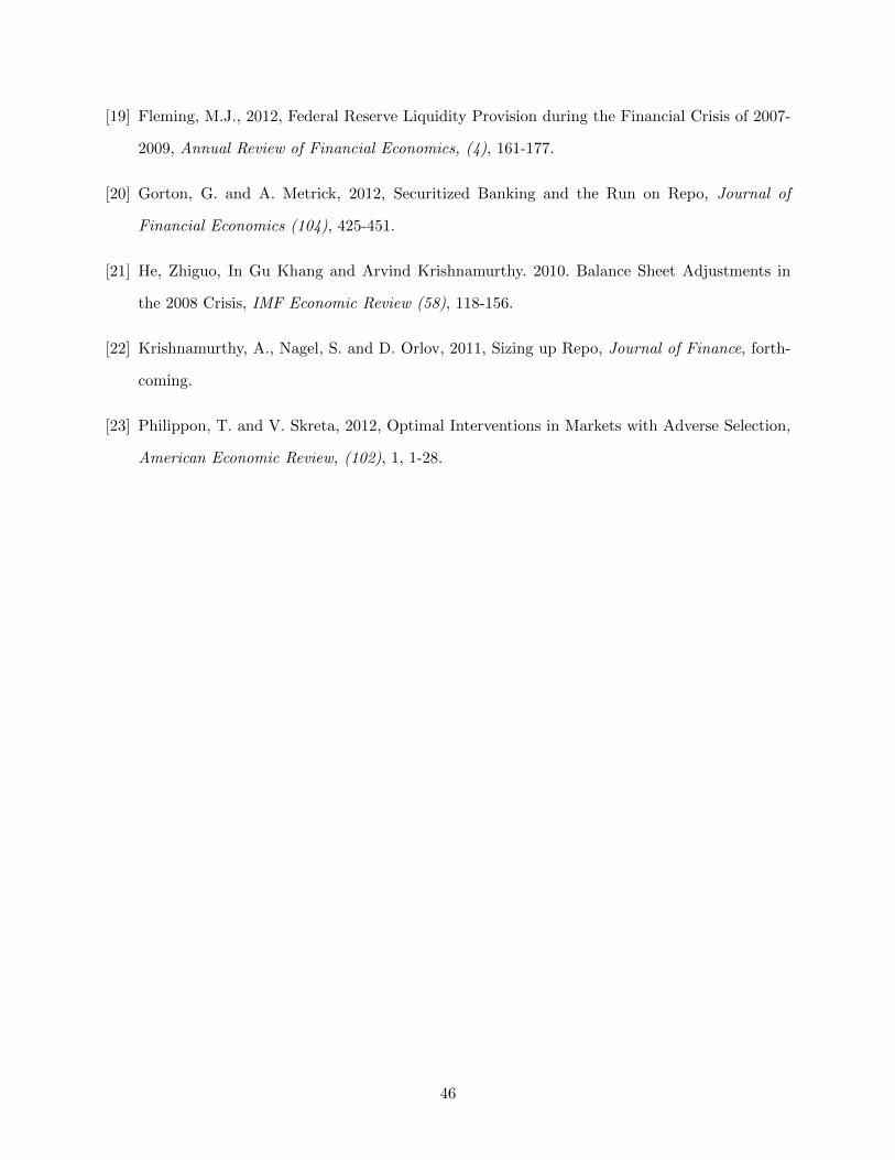
[19] Fleming, M.J., 2012, Federal Reserve Liquidity Provision during the Financial Crisis of 2007-

2009, Annual Review of Financial Economics, (4), 161-177.

[20] Gorton, G. and A. Metrick, 2012, Securitized Banking and the Run on Repo, Journal of

Financial Economics (104), 425-451.

[21] He, Zhiguo, In Gu Khang and Arvind Krishnamurthy. 2010. Balance Sheet Adjustments in

the 2008 Crisis, IMF Economic Review (58), 118-156.

[22] Krishnamurthy, A., Nagel, S. and D. Orlov, 2011, Sizing up Repo, Journal of Finance, forth-

coming.

[23] Philippon, T. and V. Skreta, 2012, Optimal Interventions in Markets with Adverse Selection,

American Economic Review, (102), 1, 1-28.

46

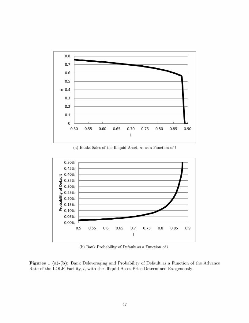
0

0.1

0.2

0.3

0.4

0.5

0.6

0.7

0.8

0.50 0.55 0.60 0.65 0.70 0.75 0.80 0.85 0.90

α

l

(a) Banks Sales of the Illiquid Asset, α, as a Function of l

0.00%

0.05%

0.10%

0.15%

0.20%

0.25%

0.30%

0.35%

0.40%

0.45%

0.50%

0.5 0.55 0.6 0.65 0.7 0.75 0.8 0.85 0.9

Pro

ba

bil

ity

of

De

fau

lt

l

(b) Bank Probability of Default as a Function of l

Figures 1 (a)-(b): Bank Deleveraging and Probability of Default as a Function of the AdvanceRate of the LOLR Facility, l, with the Illiquid Asset Price Determined Exogenously

47

0.0

0.1

0.2

0.3

0.4

0.5

0.6

0.7

0.8

0 2.5 5 7.5 10 12.5 15

α

Leverage

(a) Banks Sales of the Illiquid Asset, α, as a Function ofLeverage

0.00%

0.05%

0.10%

0.15%

0.20%

0.25%

0.30%

0 2.5 5 7.5 10 12.5 15

Pro

ba

bil

ity

of

De

fau

lt

Leverage

(b) Bank Probability of Default as a Function of Leverage(Truncated Vertical Axis)

0%

20%

40%

60%

0 2.5 5 7.5 10 12.5 15

Pro

ba

bil

ity

of

De

fau

lt

Leverage

(c) Bank Probability of Default as a Function of Leverage(Full Vertical Axis)

Figures 2 (a)-(c): Bank Deleveraging and Probability of Default as a Function of Leverage, withthe Illiquid Asset Price Determined Exogenously

48

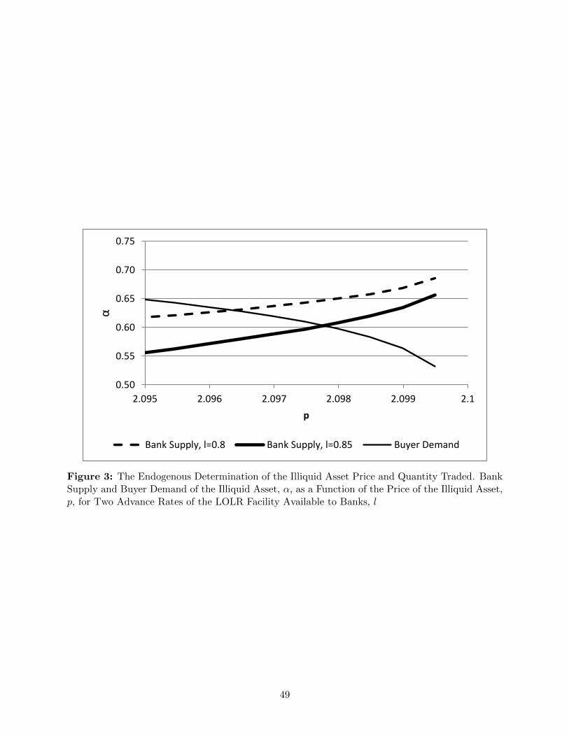
0.50

0.55

0.60

0.65

0.70

0.75

2.095 2.096 2.097 2.098 2.099 2.1

α

p

Bank Supply, l=0.8 Bank Supply, l=0.85 Buyer Demand

Figure 3: The Endogenous Determination of the Illiquid Asset Price and Quantity Traded. BankSupply and Buyer Demand of the Illiquid Asset, α, as a Function of the Price of the Illiquid Asset,p, for Two Advance Rates of the LOLR Facility Available to Banks, l

49

2.080

2.085

2.090

2.095

2.100

0.50 0.55 0.60 0.65 0.70 0.75 0.80 0.85 0.90

p

l

(a) The Equilibrium Illiquid Asset Price, p, as a Functionof the LOLR Facility Advance Rate Available to Banks, l

0.50

0.55

0.60

0.65

0.70

0.75

0.50 0.60 0.70 0.80 0.90

α

l

(b) The Equilibrium Quantity Traded of the Illiquid As-set, α, as a Function of the LOLR Facility Advance RateAvailable to Banks, l

0.00%

0.05%

0.10%

0.15%

0.20%

0.25%

0.30%

0.35%

0.50 0.55 0.60 0.65 0.70 0.75 0.80 0.85 0.90

Pro

ba

bil

ity

of

De

fau

lt

l

Bank Buyer

(c) The Probability of Bank and Buyer Default as a Func-tion of the LOLR Facility Advance Rate Available to Banks,l

Figures 4 (a)-(c): The Effect of the LOLR Facility Advance Rate Available to Banks, l, on theEquilibrium Illiquid Asset Price, p, the Equilibrium Quantity Traded of the Illiquid Asset, α, andthe Bank and Buyer Probabilities of Default 50

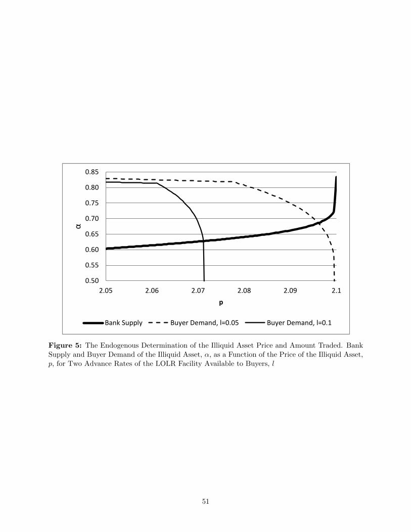
0.50

0.55

0.60

0.65

0.70

0.75

0.80

0.85

2.05 2.06 2.07 2.08 2.09 2.1

α

p

Bank Supply Buyer Demand, l=0.05 Buyer Demand, l=0.1

Figure 5: The Endogenous Determination of the Illiquid Asset Price and Amount Traded. BankSupply and Buyer Demand of the Illiquid Asset, α, as a Function of the Price of the Illiquid Asset,p, for Two Advance Rates of the LOLR Facility Available to Buyers, l

51

2.090

2.093

2.095

2.098

2.100

0.00 0.10 0.20 0.30 0.40 0.50

p

l

(a) The Equilibrium Illiquid Asset Price, p, as a Functionof the LOLR Facility Advance Rate Available to Buyers, l

0.65

0.70

0.75

0.80

0.00 0.10 0.20 0.30 0.40 0.50

α

l

(b) The Equilibrium Quantity Traded of the Illiquid As-set, α, as a Function of the LOLR Facility Advance RateAvailable to Buyers, l

0.00%

0.02%

0.04%

0.06%

0.08%

0.10%

0.12%

0.14%

0.16%

0.18%

0.20%

0.00 0.10 0.20 0.30 0.40 0.50

Pro

ba

bil

ity

of

De

fau

lt

l

Bank Buyer

(c) Insert subaption 6c here

Figures 6 (a)-(c): The Effect of the LOLR Facility Advance Rate Available to Buyers, l, on theEquilibrium Illiquid Asset Price, p, the Equilibrium Quantity Traded of the Illiquid Asset, α, andthe Bank and Buyer Probabilities of Default

52

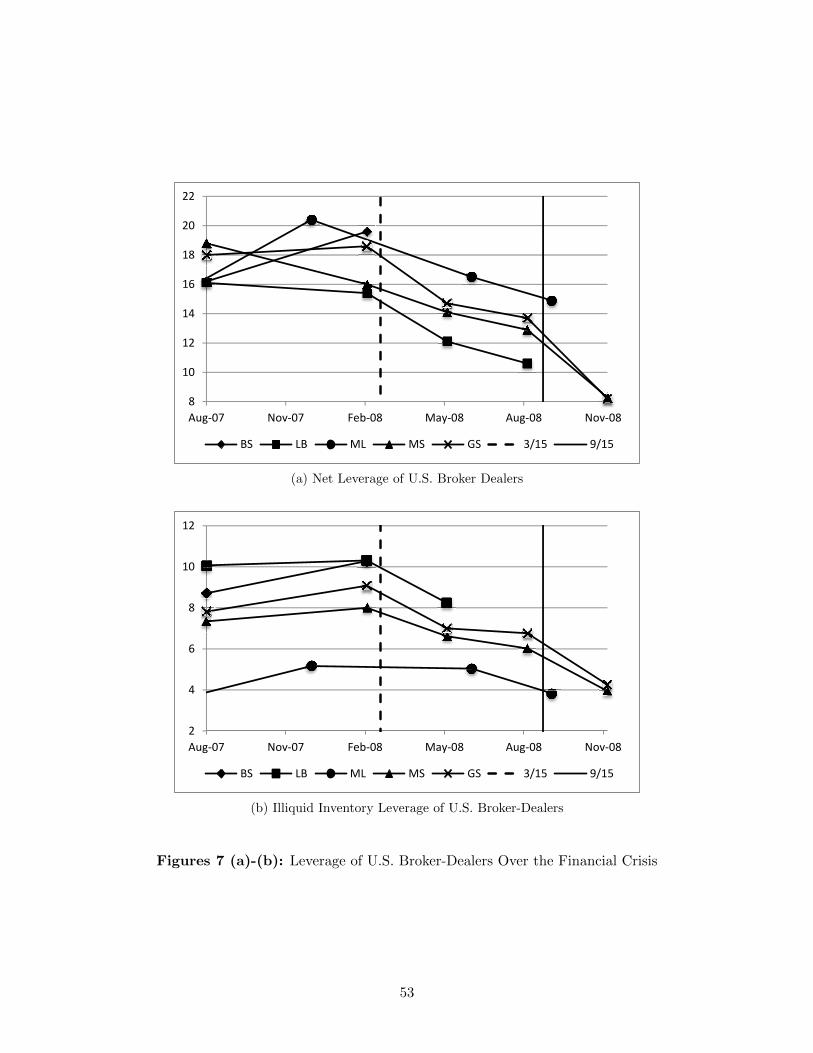
8

10

12

14

16

18

20

22

Aug-07 Nov-07 Feb-08 May-08 Aug-08 Nov-08

BS LB ML MS GS 3/15 9/15

(a) Net Leverage of U.S. Broker Dealers

2

4

6

8

10

12

Aug-07 Nov-07 Feb-08 May-08 Aug-08 Nov-08

BS LB ML MS GS 3/15 9/15

(b) Illiquid Inventory Leverage of U.S. Broker-Dealers

Figures 7 (a)-(b): Leverage of U.S. Broker-Dealers Over the Financial Crisis

53

-3

-2

-1

0

1

2

3

-100 -50 0 50 100 150 200 250

Ch

an

ge

Ill

iqu

id L

ev

era

ge

Change in CDS

LB MS GS ML BS

(a) Change in Illiquid Inventory Leverage vs. Change in CDS Spread for U.S.Broker Dealers, by Broker-Dealer

-3

-2

-1

0

1

2

3

-100 -50 0 50 100 150 200 250

Ch

an

ge

in

Ill

iqu

id L

ev

era

ge

Change in CDS

Q1 2008 Q2 2008 Q3 2008 Q4 2008

(b) Change in Illiquid Inventory Leverage vs. Change in CDS Spread for U.S.Broker Dealers, By Quarter

Figures 8 (a)-(b): Change in Illiquid Inventory Leverage vs. Change in CDS Spread for U.S.Broker Dealers

54

0%

5%

10%

15%

20%

25%

30%

Q2 2008 Q3 2008 Q4 2008

Ma

x L

OLR

Usa

ge

/ I

nv

en

tory

LB ML MS GS

Figure 9: Maximum Combined Usage of TSLF and PDCF as a % of Inventory, by Quarter

0%

5%

10%

15%

20%

25%

30%

0 100 200 300 400 500 600

Usa

ge

as

a %

of

Inv

en

tory

CDS Spread

Q2 2008 Q3 2008 Q4 2008

Figure 10: Maximum Combined Usage of TSLF and PDCF as a % of Inventory vs. CDS Spread

55

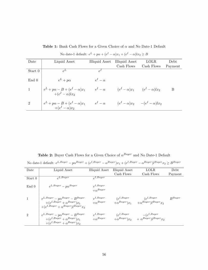
Table 1: Bank Cash Flows for a Given Choice of α and No Date-1 Default

No date-1 default: eL + pα+ (eI − α)x1 + (eI − α)lx2 ≥ B

Date Liquid Asset Illiquid Asset Illiquid Asset LOLR DebtCash Flows Cash Flows Payment

Start 0 eL eI

End 0 eL + pα eI − α

1 eL + pα−B + (eI − α)x1 eI − α (eI − α)x1 (eI − α)lx2 B+(eI − α)lx2

2 eL + pα−B + (eI − α)x1 eI − α (eI − α)x2 −(eI − α)lx2+(eI − α)x2

Table 2: Buyer Cash Flows for a Given Choice of αBuyer and No Date-1 Default

No date-1 default: eL,Buyer − pαBuyer + (eI,Buyer − αBuyer)x1 + (eI,Buyer − αBuyer)lBuyerx2 ≥ BBuyer

Date Liquid Asset Illiquid Asset Illiquid Asset LOLR DebtCash Flows Cash Flows Payment

Start 0 eL,Buyer eI,Buyer

End 0 eL,Buyer − pαBuyer eI,Buyer

+αBuyer

1 eL,Buyer − pαBuyer −BBuyer eI,Buyer (eI,Buyer (eI,Buyer BBuyer

+(eI,Buyer + αBuyer)x1 +αBuyer +αBuyer)x1 +αBuyer)lBuyerx2+(eI,Buyer + αBuyer)lBuyerx2

2 eL,Buyer − pαBuyer −BBuyer eI,Buyer (eI,Buyer −(eI,Buyer

+(eI,Buyer + αBuyer)x1 +αBuyer +αBuyer)x2 + αBuyer)lBuyerx2+(eI,Buyer + αBuyer)x2

56

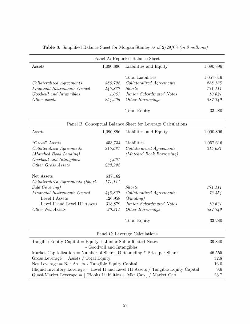
Table 3: Simplified Balance Sheet for Morgan Stanley as of 2/29/08 (in $ millions)

Panel A: Reported Balance Sheet

Assets 1,090,896 Liabilities and Equity 1,090,896

Total Liabilities 1,057,616Collateralized Agreements 386,792 Collateralized Agreements 288,135Financial Instruments Owned 445,837 Shorts 171,111Goodwill and Intangibles 4,061 Junior Subordinated Notes 10,621Other assets 254,206 Other Borrowings 587,749

Total Equity 33,280

Panel B: Conceptual Balance Sheet for Leverage Calculations

Assets 1,090,896 Liabilities and Equity 1,090,896

“Gross” Assets 453,734 Liabilities 1,057,616Collateralized Agreements 215,681 Collateralized Agreements 215,681(Matched Book Lending) (Matched Book Borrowing)Goodwill and Intangibles 4,061Other Gross Assets 233,992

Net Assets 637,162Collateralized Agreements (Short- 171,111Sale Covering) Shorts 171,111Financial Instruments Owned 445,837 Collateralized Agreements 72,454

Level I Assets 126,958 (Funding)Level II and Level III Assets 318,879 Junior Subordinated Notes 10,621

Other Net Assets 20,214 Other Borrowings 587,749

Total Equity 33,280

Panel C: Leverage Calculations

Tangible Equity Capital = Equity + Junior Subordinated Notes 39,840- Goodwill and Intangibles

Market Capitalization = Number of Shares Outstanding * Price per Share 46,555Gross Leverage = Assets / Total Equity 32.8Net Leverage = Net Assets / Tangible Equity Capital 16.0Illiquid Inventory Leverage = Level II and Level III Assets / Tangible Equity Capital 9.6Quasi-Market Leverage = [ (Book) Liabilities + Mkt Cap ] / Market Cap 23.7

57

Table

4:

Bal

ance

Sh

eet

and

Lev

erag

eC

omp

onen

tsof

the

Ma

jor

Inves

tmen

tB

anks

Fro

m8/

07to

11/0

8

Bal

ance

shee

tan

dle

vera

geco

mp

onen

tsar

ein

$m

illi

on

s.Il

liqu

idin

vento

ryis

defi

ned

as

Tota

lF

inan

cial

Inst

rum

ents

Ow

ned

-L

evel

IA

sset

s.

Pan

elA

:B

ear

Ste

arn

s

8/31/

2007

2/29/

2008

%C

han

geA

sset

s39

7,0

9139

8,99

50.

5N

etA

sset

s213

,442

220

,053

3.1

Inve

nto

ry141,

874

141,

104

-0.5

Lev

elI

Ass

ets

27,

140

25,6

90-5

.3Il

liqu

idIn

ven

tory

114,7

3411

5,41

40.

6T

ota

lE

qu

ity

13,0

00

11,

896

-8.5

Tan

gib

leE

qu

ity

13,1

7211,

224

-14.

8M

ark

etC

ap

15,7

10

11,6

33-2

6.0

Pan

elB

:L

ehm

anB

roth

ers

8/31/

2007

2/29/

2008

%C

han

ge5/

30/2

008

%C

han

geA

sset

s65

9,2

1678

6,03

519

.263

9,43

2-1

8.7

Net

Ass

ets

357

,102

396

,673

11.1

327,

774

-17.

4In

vento

ry302,

297

326,

658

8.1

269,

409

-17.

5L

evel

IA

sset

s79,

154

61,7

57-2

2.0

45,5

65-2

6.2

Illi

qu

idIn

ven

tory

223,1

4326

4,90

118

.722

3,84

4-1

5.5

Tota

lE

qu

ity

21,7

33

24,

832

14.3

26,2

765.

8T

an

gib

leE

qu

ity

22,1

6425,

696

15.9

27,1

795.

8M

ark

etC

ap

29,0

29

28,1

15-3

.120

,345

-27.

6

Pan

elC

:M

erri

llL

yn

ch

6/29/

2007

12/28/

2007

%C

han

ge6/

27/2

008

%C

han

ge9/

26/2

008

%C

han

geA

sset

s1,0

76,3

24

1,0

20,

050

-5.2

966,

210

-5.3

875,

780

-9.4

Net

Ass

ets

610

,131

642

,525

5.3

569,

103

-11.

456

7,40

6-0

.3In

vento

ry224,

789

234,

669

4.4

217,

639

-7.3

189,

358

-13.

0L

evel

IA

sset

s88,

623

71,6

84-1

9.1

43,8

14-3

8.9

43,1

57-1

.5Il

liqu

idIn

ven

tory

136,1

6616

2,98

519

.717

3,82

56.

714

6,20

1-1

5.9

Tota

lE

qu

ity

42,1

91

31,

932

-24.

334

,778

8.9

38,3

5510

.3T

an

gib

leE

qu

ity

42,5

2331,

566

-25.

834

,484

9.2

38,1

3910

.6M

ark

etC

ap

72,0

47

50,3

84-3

0.1

32,2

21-3

6.0

43,7

7835

.9

58

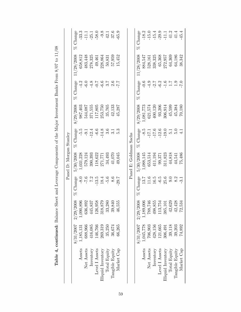
Table

4,continued:

Bala

nce

Sh

eet

and

Lev

erag

eC

omp

onen

tsof

the

Majo

rIn

vest

men

tB

anks

Fro

m8/

07to

11/0

8

Pan

elD

:M

orga

nS

tan

ley

8/31/

2007

2/29/2

008

%C

han

ge5/

30/2

008

%C

han

ge8/

29/2

008

%C

han

ge11

/28/

2008

%C

han

geA

sset

s1,

185,1

31

1,09

0,8

96-8

.01,

031,

228

-5.5

987,

403

-4.2

658,

812

-33.

3N

etA

sset

s688

,966

636,

892

-7.6

579,

124

-9.1

544,

087

-6.0

483,

448

-11.

1In

vento

ry416,

085

445,8

377.

239

0,39

3-1

2.4

371,

555

-4.8

278,

325

-25.

1L

evel

IA

sset

s146,

766

126,9

58-1

3.5

118,

622

-6.6

117,

805

-0.7

49,4

61-5

8.0

Illi

qu

idIn

ven

tory

269,3

1931

8,8

79

18.4

271,

771

-14.

825

3,75

0-6

.622

8,86

4-9

.8T

ota

lE

qu

ity

35,2

50

33,2

80

-5.6

34,4

933.

635

,765

3.7

50,8

3142

.1T

angib

leE

qu

ity

36,

674

39,8

408.

641

,070

3.1

42,1

332.

657

,959

37.6

Mark

etC

ap

66,2

65

46,

555

-29.

749

,045

5.3

45,2

87-7

.715

,452

-65.

9

Pan

elE

:G

old

man

Sac

hs

8/31/

2007

2/29/2

008

%C

han

ge5/

30/2

008

%C

han

ge8/

29/2

008

%C

han

ge11

/28/

2008

%C

han

geA

sset

s1,

045,7

78

1,18

9,0

0613

.71,

088,

145

-8.5

1,08

1,77

3-0

.688

4,54

7-1

8.2

Net

Ass

ets

706

,903

788,

746

11.6

653,

514

-17.

162

1,57

4-4

.952

8,16

1-1

5.0

Inve

nto

ry428,

156

498,8

5516

.541

1,19

4-1

7.6

400,

120

-2.7

338,

325

-15.

4L

evel

IA

sset

s121,

665

113,7

54-6

.599

,371

-12.

693

,206

-6.2

65,3

68-2

9.9

Illi

qu

idIn

ven

tory

306,4

9138

5,1

01

25.6

311,

823

-19.

030

6,91

4-1

.627

2,95

7-1

1.1

Tota

lE

qu

ity

39,1

18

42,6

29

9.0

44,8

185.

145

,599

1.7

64,3

6941

.2T

angib

leE

qu

ity

39,

203

42,4

288.

244

,541

5.0

45,3

841.

964

,186

41.4

Mark

etC

ap

74,8

92

72,

534

-3.1

75,4

864.

170

,180

-7.0

38,3

42-4

5.4

59

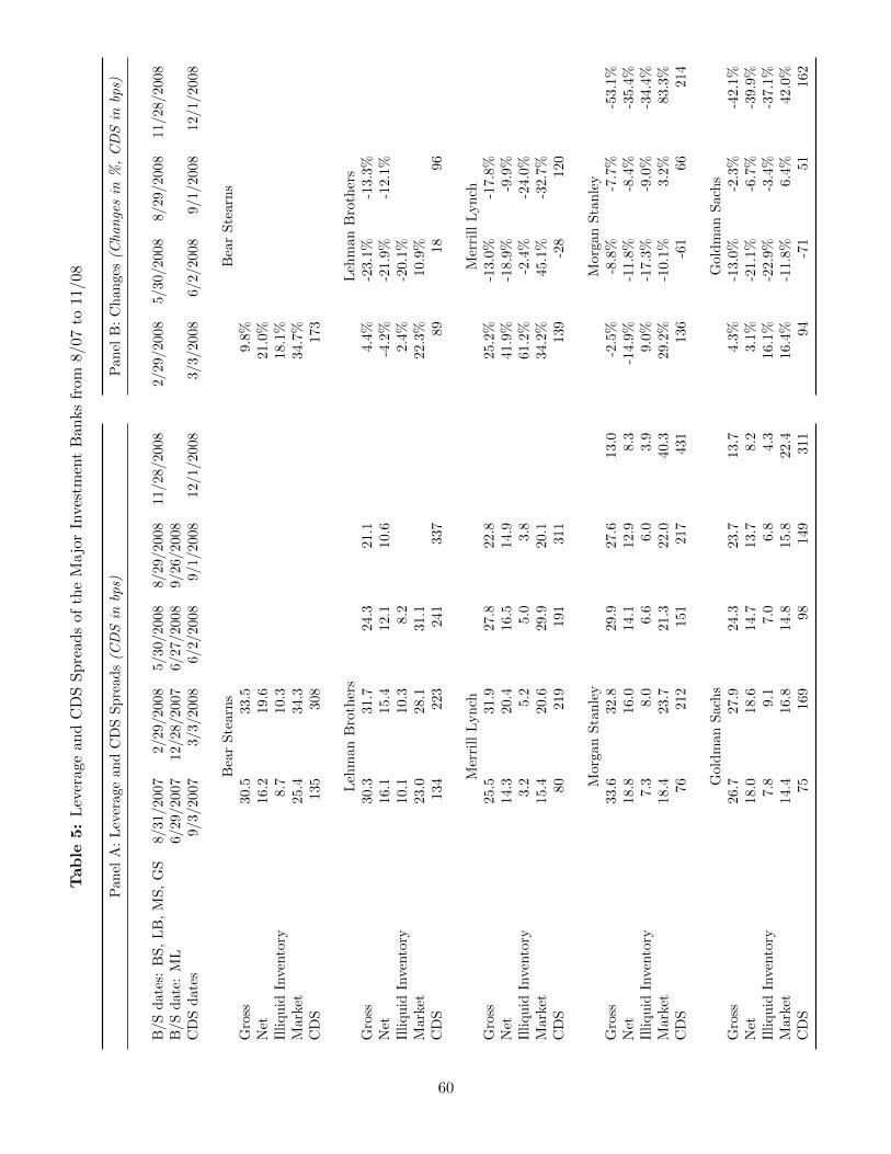
Table

5:

Lev

erage

and

CD

SS

pre

ads

ofth

eM

ajo

rIn

vest

men

tB

anks

from

8/07

to11

/08

Pan

elA

:L

ever

age

and

CD

SS

pre

ad

s(C

DSin

bps)

B/S

dat

es:

BS

,L

B,

MS

,G

S8/

31/2

007

2/29/2008

5/30/2008

8/29/2008

11/28/2008

B/S

dat

e:M

L6/

29/2

007

12/28/2007

6/27/2008

9/26/2008

CD

Sd

ates

9/3/

2007

3/3/2008

6/2/2008

9/1/2008

12/1/2008

Bea

rS

tearn

sG

ross

30.5

33.5

Net

16.2

19.6

Illi

qu

idIn

ven

tory

8.7

10.3

Mar

ket

25.4

34.3

CD

S13

5308

Leh

man

Bro

ther

sG

ross

30.3

31.7

24.3

21.1

Net

16.1

15.4

12.1

10.6

Illi

qu

idIn

ven

tory

10.1

10.3

8.2

Mar

ket

23.0

28.1

31.1

CD

S13

4223

241

337

Mer

rill

Lyn

chG

ross

25.5

31.9

27.8

22.8

Net

14.3

20.4

16.5

14.9

Illi

qu

idIn

ven

tory

3.2

5.2

5.0

3.8

Mar

ket

15.4

20.6

29.9

20.1

CD

S80

219

191

311

Mor

gan

Sta

nle

yG

ross

33.6

32.8

29.9

27.6

13.0

Net

18.8

16.0

14.1

12.9

8.3

Illi

qu

idIn

ven

tory

7.3

8.0

6.6

6.0

3.9

Mar

ket

18.4

23.7

21.3

22.0

40.3

CD

S76

212

151

217

431

Gol

dm

an

Sach

sG

ross

26.7

27.9

24.3

23.7

13.7

Net

18.0

18.6

14.7

13.7

8.2

Illi

qu

idIn

ven

tory

7.8

9.1

7.0

6.8

4.3

Mar

ket

14.4

16.8

14.8

15.8

22.4

CD

S75

169

98

149

311

Pan

elB

:C

han

ges

(Changesin

%,CDSin

bps)

2/29/2008

5/30/2008

8/29/2008

11/28/2008

3/3/2008

6/2/2008

9/1/2008

12/1/2008

Bea

rS

tearn

s9.8

%21.0

%18.1

%34.7

%173

Leh

man

Bro

ther

s4.4

%-2

3.1

%-1

3.3

%-4

.2%

-21.9

%-1

2.1

%2.4

%-2

0.1

%22.3

%10.9

%89

18

96

Mer

rill

Lyn

ch25.2

%-1

3.0

%-1

7.8

%41.9

%-1

8.9

%-9

.9%

61.2

%-2

.4%

-24.0

%34.2

%45.1

%-3

2.7

%139

-28

120

Morg

an

Sta

nle

y-2

.5%

-8.8

%-7

.7%

-53.1

%-1

4.9

%-1

1.8

%-8

.4%

-35.4

%9.0

%-1

7.3

%-9

.0%

-34.4

%29.2

%-1

0.1

%3.2

%83.3

%136

-61

66

214

Gold

man

Sach

s4.3

%-1

3.0

%-2

.3%

-42.1

%3.1

%-2

1.1

%-6

.7%

-39.9

%16.1

%-2

2.9

%-3

.4%

-37.1

%16.4

%-1

1.8

%6.4

%42.0

%94

-71

51

162

60

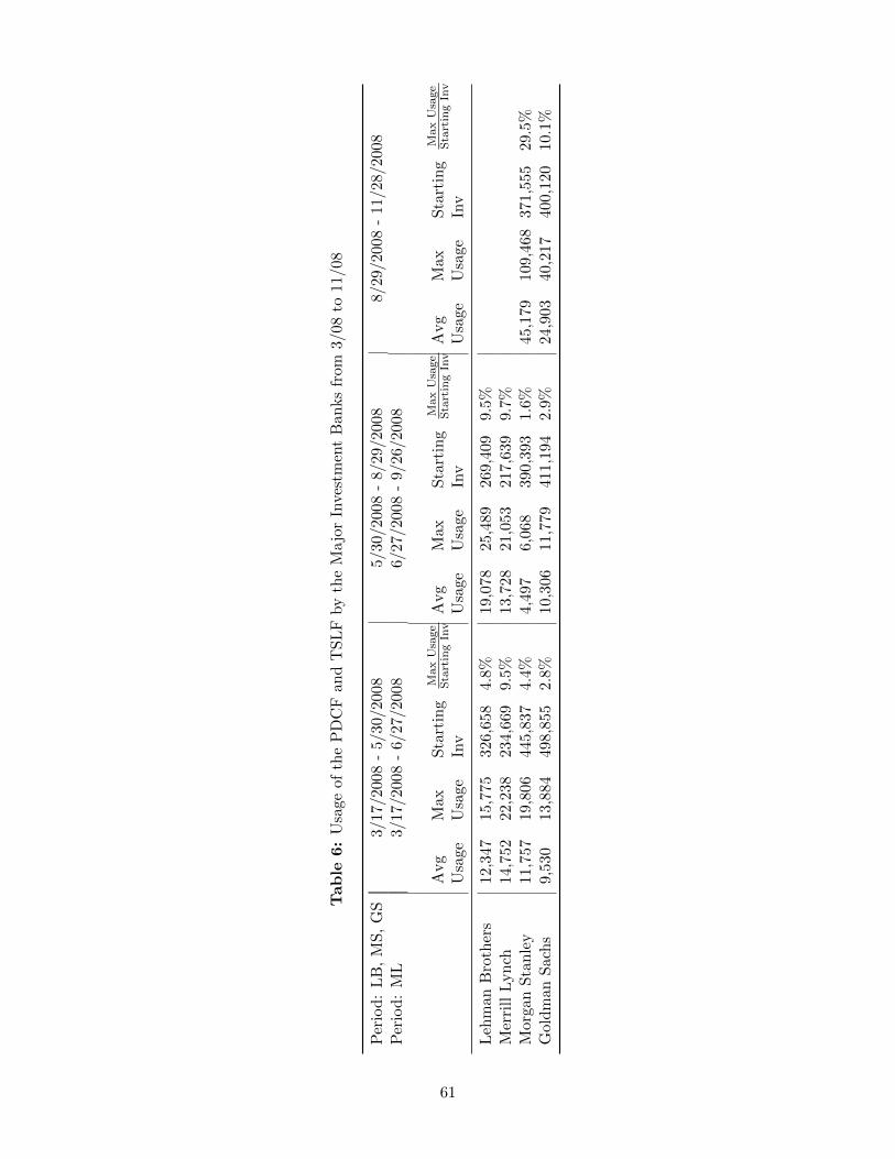
Table

6:

Usa

ge

of

the

PD

CF

and

TS

LF

by

the

Majo

rIn

vest

men

tB

anks

from

3/08

to11

/08

Per

iod

:L

B,

MS

,G

S3/17

/200

8-

5/30

/200

85/

30/2

008

-8/

29/2

008

8/29

/200

8-

11/2

8/20

08P

erio

d:

ML

3/17

/200

8-

6/27

/200

86/

27/2

008

-9/

26/2

008

Avg

Usa

ge

Max

Usa

ge

Sta

rtin

gIn

v

MaxUsage

StartingInv

Avg

Usa

geM

axU

sage

Sta

rtin

gIn

v

MaxUsage

StartingInv

Avg

Usa

geM

axU

sage

Sta

rtin

gIn

v

MaxUsage

StartingInv

Leh

man

Bro

ther

s12

,347

15,7

75

326,

658

4.8%

19,0

7825

,489

269,

409

9.5%

Mer

rill

Lyn

ch14

,752

22,2

38

234,

669

9.5%

13,7

2821

,053

217,

639

9.7%

Mor

gan

Sta

nle

y11

,757

19,8

06

445,

837

4.4%

4,49

76,

068

390,

393

1.6%

45,1

7910

9,46

837

1,55

529

.5%

Gol

dm

anS

ach

s9,

530

13,8

84

498,

855

2.8%

10,3

0611

,779

411,

194

2.9%

24,9

0340

,217

400,

120

10.1

%

61