Unified Representation and Lifted Sampling forGenerative Models of Social Networks

Pablo Robles-Granda1, Sebastian Moreno2, and Jennifer Neville11Department of Computer Science, Purdue University

2Faculty of Engineering and Science, Universidad Adolfo Ibanez1{problesg,neville}@purdue.edu, 2sebastian.moreno@uai.cl

AbstractStatistical models of network structure are widelyused in network science to reason about the prop-erties of complex systems—where the nodes andedges represent entities and their relationships. Re-cently, a number of generative network models(GNM) have been developed that accurately capturecharacteristics of real world networks, but since theyare typically defined in a procedural manner, it isdifficult to identify commonalities in their structure.Moreover, procedural definitions make it difficult todevelop statistical sampling algorithms that are bothefficient and correct. In this paper, we identify a fam-ily of GNMs that share a common latent structureand create a Bayesian network (BN) representationthat captures their common form. We show howto reduce two existing GNMs to this representation.Then, using the BN representation we develop a gen-eralized, efficient, and provably correct, samplingmethod that exploits parametric symmetries and de-terministic context-specific dependence. Finally, weuse the new representation to design a novel GNMand evaluate it empirically.

1 IntroductionMany complex systems are modeled using networks—wherenodes represent entities and edges represent some type ofrelation between the entities. An open problem in networkscience is how to create generative models that accuratelycapture the characteristics of real world, sparse networks, inorder to better understand the properties of the systems, andto facilitate statistical analysis.

Recent research has explored various models to accuratelycharacterize network structure (e.g., [Chung and Lu, 2002;Hoff, 2008; Leskovec et al., 2010; Benson et al., 2014]). Anumber of these generative network models (GNMs) use acommon procedure to generate the edges in the network usinga matrix of probabilities. The approaches differ in the numberand structure of parameters used to specify the edge probabili-ties. While several GNMs can capture important characteris-tics of real world networks such as power law degree distribu-tions and community structure, it has been more difficult todevelop methods to capture longer-range dependencies that im-

pact global characteristics. To address these limitations, newhierarchical GNMs have been proposed with more complexdependencies between the edge probabilities, e.g., mixed Kro-necker product graph model (mKPGM) [Moreno et al., 2013],Block two-level Erdos-Renyi Model (BTER) [Seshadhri et al.,2012], bipartite stochastic block model (biSBM) [Larremoreet al., 2014], and hierarchical graph models [Peixoto, 2014].

Moreover, while GNMs specify a generative process, itcan still be computationally intensive to naively sample largenetworks. There have been efficient sampling methods pro-posed for some GNMs [Leskovec et al., 2010; Yun and Vish-wanathan, 2012], but because models are specified procedu-rally it is difficult to guarantee correctness, and consequentlythe efficient sampling methods can generate improbable net-work structures [Moreno et al., 2014]. Thus, it is still an openquestion how to develop accurate and efficient sampling meth-ods. Another challenge is to identify commonalities acrossGNMs. Again, since models are specified procedurally, it isdifficult to discern the impact of algorithmic differences–bothw.r.t. the number and structure of parameters–except by com-paring the structure of the networks that are generated fromthe methods.

In this paper, we show that hierarchical GNMs can beabstracted as Bayesian networks (BNs) with random vari-ables (RVs) representing the existence of edges in the net-work, and hierarchies of latent RVs representing relationsamong groups of edges. With this representation we canidentify common properties of unrelated models, such asmKPGM and BTER, and use the knowledge to guide thedesign of new GNMs. The BN representation also facili-tates the development of a general sampling method that isboth efficient and accurate. The transformation of a GNMto BN representation makes it easy to identify parametricsymmetries allowing us to sample groups of edge RVs ratherthan sequentially—using insights from lifted inference [Poole,2003; Jha et al., 2010; Van den Broeck and Darwiche, 2013;Mittal et al., 2015]. Moreover, we can maximize computa-tional efficiency and guarantee correctness by using insightsfrom context specific independence [Boutilier et al., 1996;Poole and Zhang, 2003] to dynamically sparsify the set of RVsto be sampled based on the context of parent RV values.

Previous work had provided important insights about therelationship among some GNMs (e.g. [Jacobs and Clauset,2014]) and BNs have been used to model GNMs (e.g.

[Schein et al., 2016; Liang et al., 2016; Ho et al., 2011;Neiswanger et al., 2014]), However, to our knowledge, thiswork is the first attempt to model a family of existing GNMsin a principled way that is general enough to facilitate thecreation of new classes of GNMs. We do that by taking advan-tage of BNs to model GNMs but without enforcing restrictionson the topology of a BN except for a hierarchical conditionaldependence which we describe in this paper.

In summary, the key contributions of this work are:

1. Demonstration that hierarchical GNMs can be representedin a universal, succinct way that supports the developmentof new models.

2. Development of a general efficient, and provably correct,sampling algorithm that applies to all GNMs in the familyof hierarchical GNMs. Our algorithm is based on twoimportant properties:

(a) Deterministic context specific dependence–which spar-sifies the RV sampling space.

(b) Parametric symmetries–which, due to GNM parame-terizations, can be exploited with lifted sampling.

3. Design, and evaluation, of a new GNM to illustrate theutility of the BN representation; in particular, of the relatedsampling algorithm.

2 Background: Generative Network ModelsFirst, we review some details about generative network models.Let G=(V,E) be a network with set of vertices V and edgesE ⊂ V ×V. We define a generative network model (GNM)M with parameters Θ as follows.

Definition 1. Generative network model (GNM)A GNM is a statistical modelM with parameters Θ that define,either explicitly or via a construction process, a size |V|× |V|matrix P of probabilities. Each cell [i, j] ∈ P corresponds tothe binary random variable Aij and the value Pij representsthe Bernoulli probability that the [un]directed edge ei,j existsin the network (i.e., ifAij=1 then ei,j ∈ E and P (Aij=1) =Pij). Thus, P models the structure of the network through theset of binary random variables Aij ∀i, j ∈ {1, . . . , |V|}.

The size of Θ differs for each GNM and can vary in therange [1, |V|2]. This restriction in the number of parame-ters is intended to make sampling of random graphs effi-cient. However, most GNMs have a small number of param-eters (usually |Θ|�|V|) to avoid overfitting. Thus, multiplecells in P (and RVs A) could have the same probability val-ues. We use < U,T > to represent this, where U is theset of unique probabilities that appear in the matrix P , i.e.U=unique(P)={π1, π2, . . . , πu , . . . πκ}, and T is the setof the list of positions Tuwhere each of the πu appears in P .

2.1 Basic Edge-Oriented GNMsThere is a range of basic GNMs such as Erdos-Renyi Model(ER) [Erdos and Renyi, 1960], Stochastic Block Model(SBM) [Holland et al., 1983], Chung-Lu Model (CL) [Chungand Lu, 2002], etc. that build P with some mathematical op-eration over a set of parameter(s). For space reasons we willdefine only CL here since is relevant for our later discussion.

Chung-Lu Model (CL) [Chung and Lu, 2002]. In a CLmodel, Pij=wiwj/

∑wk for a sequence of expected node-

degrees w = (w1,. . ., w|V|). There are then, for the case ofundirected networks, at most |V|(|V|−1)/2 probabilities πiin P (and associated U), in which case T would consist oflists of a single element each.

2.2 Hierarchical GNMsHierarchical GNMs are a super-classs of GNMs that use ahierarchical process to introduce dependencies among sets ofedge RVs. While a basic GNM defines the matrix P directly,a hierarchical GNM uses intermediate latent variables at acertain level in the hierarchy to model the variable interactionsof the next level in the hierarchy, modeling the entries in Pindirectly. Thus, there are two levels of randomness associatedwith sampling in hierarchical GNMs: one for the intermediate(hierarchical) RVs that impact the generation of P , and onefor edge sampling. Notice that basic GNMs can be regardedas hierarchical GNMs with a single layer. Most hierarchicalGNMs are defined iteratively or procedurally, but not all it-erative or procedural GNMs are hierarchical. We denote thelevels in the hierarchy by λ ∈ {0, 1, . . . , φ − 1}, where φ isthe number of levels in the hierarchy, λ=0 represents the rootof the hierarchy, and λ = φ − 1 the edge layer. B[λ] is theadjacency matrix associated with the blocks at layer λ.

Block two-level Erdos-Renyi Model (BTER) [Seshadhri etal., 2012]. In a preprocessing step, BTER creates groupsof nodes based on the sequence of expected degrees. Then,sampling is done in two steps: (1) An ER model is used tolink nodes within groups, where the probability is proportionalto the smallest node-degree in the group; (2) A CL model isused to create link between groups, with probability of edgesis proportional to the excess degree from (1). Step 1 ensuresthat edges within-blocks have higher probability than between-blocks. Step 2 ensures a power law degree-distribution andsince it uses a CL model, U & T have the same worst casescenario as CL.

Mixed Kronecker Product Graph Model (mKPGM)[Moreno et al., 2013]. mKPGM is a GNM that overcomesknown limitations (see e.g. [Seshadhri et al., 2013]) of stochas-tic Kronecker graphs [Leskovec et al., 2010]. Given a b×bparameter matrix Θ, K and `, it samples a network as follows.

1. Compute P [0], a b` × b` matrix, equal to `−1 Kroneckerproducts of Θ with itself.

2. Construct G[0]from P [0] by sampling each edge RV inde-pendently ∼ Bernoulli(P [0]

ij ).

3. For l=1 . . .K−`: Set P [l] =G[l−1] ⊗Θ and sample G[l].Note, |V[0]|= b` and |V[K−`]|= bK. Since G[0]. . . G[K−−1]

represent auxiliary graphs, where each edge influences ablock of possible edges in the next iteration of the hierar-chical sampling process (and they are not present in the finaloutput network); we refer to them as block adjacency ma-trices: B[0] . . . B[K− −1]. To simplify notation we will referto the final sampled network G[K−`] = (V[K−`],E[K−`]) asG= (V,E). In mKPGMs, the size of U is b2 for each levell>0 of the hierarchy and T consists of b2 lists of edges.

Super-block level

Block level

Edge level� = 2

� = 1

� = 0

Z[1]j

Z[0]i

Auv

... ...... ... ...

Z[0]i

Z[0]j

A[0]uv

GNM Sampling(⇥){Derive latent RVs from ⇥

[Derive relations of RVs]

Use RVs to sample G

Return graph G

}

(a) (b) (c)Figure 1: Example transformation from an original GNM defined procedurally (a) to BN form (b) and its corresponding plate notation (c).

3 Representing GNMs as Bayesian NetworksIn this section, we introduce a common BN representationfor GNMs with hierarchical dependencies among the edge-probabilities, and develop an associated, efficient samplingmethod. We also identify common properties of the GNMsbased on their BN form and exploit these properties for effi-cient and provably correct sampling.

The BN representation is comprised of a hierarchical struc-ture of edges and blocks. We denote the levels in the hierarchyby λ ∈ {0, 1, . . . , φ− 1}, where φ is the number of levels inthe hierarchy, λ=0 represents the root of the hierarchy, andλ=φ−1 the edge layer. A block j at level λ has an associatedRV Z

[λ]j which represents its state: sampled (Z

[λ]j =1) or not

(Z[λ]j = 0). Since blocks could have different sizes we keep

a one dimensional subindex for each block RV (Zi) ratherthan use the rectangular structure (with two subindices Zij) ofsome GNMs (e.g., mKPGM in Fig. 2). Likewise, P could beregarded as a one-dimensional structure for this same purpose(notice that P (B

[λ]j =1) = P [λ]

j is the probability of samplingblock j as defined by the GNM). This illustrates that our algo-rithm is easily applicable to hierarchical models with complextopology of the interacting layers and not just to tree-like BNs.The function pa

(Z

[λ]j

):=Z

[λ−1]i for λ>0 returns the parent

RVs for Z [λ]j . We denote as Z[λ] the set {Z [λ]

j }. It is importantto notice that the BN is comprised of Z[0], . . . ,Z[φ−1] andthat the parameters of the BN are the associated probabilities.These probabilities are a function of, or derived from, P [λ].However, this relation is not straightforward for all GNMs.

3.1 Transformation of GNMs to BNsAs discussed in the previous section, hierarchical GNMsare a superclass of GNMs that include edge-based GNMsas a special case, as well as more complex models thatuse a hierarchy of latent variables to represent dependen-cies among edge RVs. However, since most hierarchicalGNMs are defined iteratively, the hierarchical structure isnot immediately evident and a transformation is necessary.In particular for procedural models, transforming a GNMto BN form consists of two steps, as outlined in Figure 1:(1) Restructure the output of each step in the iterative sam-pling of a GNM as a set of RVs. This allows the process tobe reorganized as levels in a hierarchy of RVs. (2) Use the

hierarchy of RVs to build a BN using parameters for the BNderived from the GNM. Some care should be exercised forthis transformation as the relations among RVs are not trivial.

General Transformation from Hierarchical GNM to BNA hierarchical model M, with parameter matrix Θ, can berepresented as a BN N with parameters Θ′ obtained from Θ:MΘ r⇀NΘ′ as follows:1. Represent as Z [0]

j the RV that models the block edge B[0]j

2. Define the probability of Z [0]j : P (Z

[0]j =1) = P [0][j]

3. For λ = 1, . . . , φ− 1

(a) Represent as Z [λ]k the RV that models the block B[λ]

k

(b) Specify pa(Z

[λ]k

)= Z

[λ−1]k′ to be the corresponding

parent of RV Z[λ]k , then, define the CPD of Z [λ]

k :P(Z

[λ]k = 1|pa

(Z

[λ]k

)= 1

)= P [λ][k]

P(Z

[λ]k = 1|pa

(Z

[λ]k

)= 0

)= 0

4. Add the RVs Z[0], . . . ,Z[φ−1] (from 1 & 3.a) to the BN Nand add their associated CPDs (from 2 & 3.b) to Θ′.

Notice that when φ (number of levels) is 1 then the hierarchicalGNM collapses to a traditional edge-based GNM. Thus, hier-archical GNMs include edge-based GNMs as a special case.Finally, Θ′ is fully defined by Θ because all P are derivedfrom it. We now discuss two specific transformations.

Transforming mKPGM to BN representation

|V[0]|

|V[0]|

|V[0]|

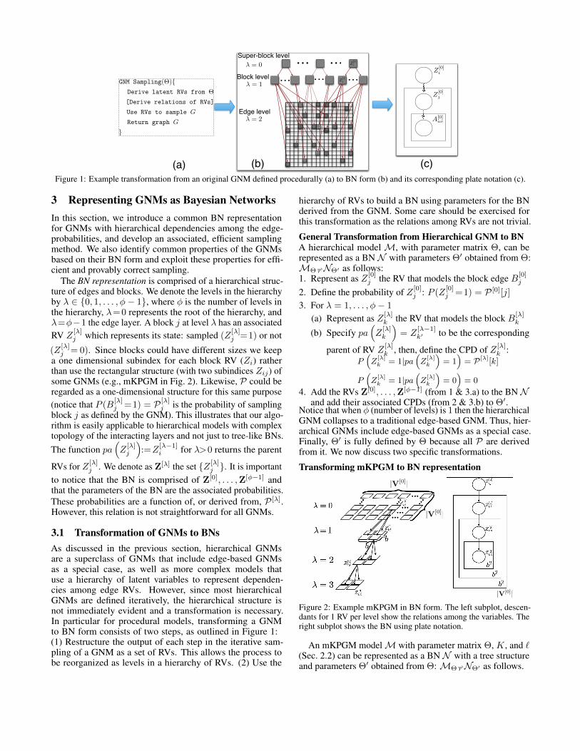
Figure 2: Example mKPGM in BN form. The left subplot, descen-dants for 1 RV per level show the relations among the variables. Theright subplot shows the BN using plate notation.

An mKPGM modelM with parameter matrix Θ, K, and `(Sec. 2.2) can be represented as a BN N with a tree structureand parameters Θ′ obtained from Θ:MΘ r⇀NΘ′ as follows.

1. Represent as Z [0]ij the RV that models the block edge B[0]

ij

∀i, j∈ [1, b`]

2. Define the CPD of Z [0]ij : P (Z

[0]ij = 1) = P [0][i, j] for all

i, j, where P [0] =⊗`k=1Θ

3. For λ = 1, . . . , φ, where φ = K − ` do:(a) Represent as Z [λ]

kl the RV that models the block edgeB

[λ]kl ∀k, l∈ [1, b`+λ]

(b) Specify pa(Z

[λ]kl

)= Z

[λ−1]dk/be,dl/be to be the parents of

RV Z[λ]kl , where x=mod (k−1, b)+1 and y=mod (l−

1, b)+ 1, then, define the CPD of Z [λ]kl , ∀k, l∈ [1, b`+λ]:

P(Z

[λ]kl = 1|pa

(Z

[λ]kl

)= 1

)= Θ[x, y]

P(Z

[λ]kl = 1|pa

(Z

[λ]kl

)= 0

)= 0

4. Add the RVs Z[0],Z[1], ...,Z[λ=K−`] (from steps 1 and 3.a)to the BN N and add their associated CPDs (from steps 2and 3.b) to Θ′.

An example BN representation of an mKPGM is shown inFig. 2 for λ=0, 1, 2, 3. Here λ=0 corresponds to B[0] in themKPGM sampling process. There is a total of (b`)2 = |V[0]|2RVs each of them represented by a Z [0]

ij (a double subindexis used to indicate the position of the RV in the block/edgematrix). Each of the RVs has b2 descendants at λ>0.

Transforming BTER to BN representationA BTER modelM with parameters Θ=({nd}d∈N, {cd}d∈N),where {nd}d∈N is a sequence of target degrees and {cd}d∈N isthe target clustering coefficient per degree, can be representedas a BN N with a tree structure and parameters Θ′ obtainedfrom Θ:MΘ r⇀NΘ′ as follows.

As discussed earlier, BTER creates groups of nodes withpossibly the same degree and uses an ER model to generateblocks of edges linking those nodes together. These are calledaffinity-blocks. To produce a power law degree distribution,there are many affinity-blocks of edges linking nodes withsmall degree and fewer blocks for nodes with larger degree.Recall that each node has an expected degree; then, bulk nodesare nodes where the minimum degree of its affinity blockis equal to its expected degree. Otherwise, if the minimumdegree is smaller, they are called filler nodes. Contrary tomKPGMs, BTER has an heterogenous number of descendentedges. The nodes of degree one have no edges between thembecause they are used as filler nodes; i.e. they are used to linkblocks of degrees > 1.

Let nb, rd, db be the number of edges in affinity block B[0]ij ,

the ratio of the number of filler nodes to the total nodes, andthe minimum degree in the block, respectively. Let, Bin−1 bethe inverse CDF of a binomial. Then, the mapping of BTERsampling to BN representation is as follows:

1. Represent as Z [0]ij the RV modeling the affinity blocks B[0]

ij

2. Obtain the parameters nb, rd, db of BTER as described inAlgorithm 1 of [Kolda et al., 2014]

3. Define the CPD of Z [0]ij : P (Z

[0]ij = 1) = P [0][i, j] ∀ i, j

where P [0] is probability of sampling edges from degreeequal to the degree of B[0]

ij

4. Let pa(·) be the affinity block containing ·. DefineP (Z

[φ]kl = 1|pa(Z

[φ]kl ) = 0) = 0 ∀k, l ∈ [1, . . . , |V|]. Oth-

erwise, for edges ek,l s.t. pa(Z[φ]kl ) = 1 and b its affinity

block with clustering coefficient cdb(a) Represent its associated RV as Z [φ]

kl

(b) If k = l: Define the CPD of Z[φ]kl :

P (Z[φ]kl =1|pa(Z

[λ]kl )=1)=Bin−1

(c1/3db

(nb2

))(c) Else: Given σtype = rd

2 if type = filler, andσtype = 1−rd

2 if type = bulk, define the CPDof Z

[φ]kl : P (Z

[φ]kl = 1|pa(Z

[λ]kl ) = 1) = Bin−1(∑

i∈Vd σtypei [di − (c1/3db· db)]

)for all k, l and nodes

i ∈ Vd of degree d

5. Add the RVs Z[0],Z[1] to the BN N (steps 1, 5.a.i, 5.b) andtheir associated CPDs (steps 3, 4, 5.a.2, & 5.c) to Θ′.

As we can see BTER and mKPGM are similar in the sensethat both models constrain the sampling so very few edgesare sampled with higher probabilities. This allows for skeweddegree distribution. The difference in the depth of the hierar-chies is now easily seen, mKPGM groups edges in blocks andsuper-blocks to abstract their relations as separate latent SBMmodels, while BTER uses shallower hierarchies for redistribu-tion of probabilities according to a power-law.

3.2 GNM-BN Common PropertiesWe identify 2 properties of GNMs transformed to BN form.1. Group Symmetries—The first key insight about our BNrepresentation is that symmetries appear in the BN fromthe parameterization of the GNM. Since there are fewerthan |V|2 unique Θs, RVs can be grouped and sampled to-gether. Moreover, since the models are designed to gener-ate sparse networks, it is more efficient to sample the num-ber of edges and then select their locations rather than se-quentially sample each edge RV, as proved in [Moreno etal., 2014]. As in earlier lifted techniques, that were basedon finding identical structures for which a common compu-tation was performed only once ([Koller and Pfeffer, 1997;Pfeffer et al., 1999]), we propose an algorithm that identifiesRVs with the same conditionals and group them together in asingle representation. Then, sampling will be done only onceby using a Binomial (this determines the number of edges tosample) and randomly selecting the edges from the locationswith the same unique probability (as illustrated in Fig. 3).Because in GNMs the symmetries are parametric similaritiesamong a set of independent RVs there is no need to assess thedependencies among individual RVs or among groups of RVs.2. DCSD Sparsification—The second property of the BNrepresentation for GMNs is deterministic context-specific de-pendence (DCSD). As seen in the earlier transformations, thisproperty arises because some values of the variables are sam-pled with value 0. Since sampling at the next layer of thehierarchy is conditional on the sampling of the previous layer,the sampling space becomes more and more sparse as wemove through the hierarchy, as shown in Figure 4. Because a

Z[1]j

Z[0]i

Auv

... ...

... ... ...pa = 0 pa = 1

P (0) 1 1�✓2

P (1) 0 ✓2

pa = 0 pa = 1P (0) 1 1�✓1

P (1) 0 ✓1

...pa = 0 pa = 1

P (0) 1 1�✓|U [2]|P (1) 0 ✓|U [2]|

Symmetries

Z[1]j

Z[0]i

Auv

... ...

... ... ...

Fill (color/blend): represent (latent) random variables (RVs) with the same value Arrows: represent dependencies among (RVs). Tables: Represent CPD of the RVs. Identifying symmetries is not a trivial task as described BN form of Fig. 1 b

Super-block level

Block level

Edge level� = 2

� = 1

� = 0

Figure 3: Sampling of GNM-BN: Symmetries of RV values are exploited for efficiency and correctness.

value in any given U[λ] may be 0, we don’t need to sample atall for the associated T . Thus this sparsification can be usedfor more efficient sampling. Formally:Definition 2. Deterministic context-specific dependence(DCSD): LetN be a BN that generates a networkG through ahierarchical sampling process. Let P

(Z

[λ]j

)be the probabil-

ity that a block is sampled. ThenN is “DCSD” iff it partitionsall Zj , such that:

P(Z

[λ]j = 1

∣∣∣pa(Z [λ]j

)= 0

)= 0 ∀ j, λ

where P(Z

[λ]j =1|pa

(Z

[λ]j

)=1

)>0 ∀ j, λ, at each layer λ.

Remark 1. Z [λ]j is sampled iff its parent is sampled with

value 1. However, if a superblock is not sampled, sam-pling of subblocks or edges is inhibited. Note that whileP (Euv|pa(Euv)=0)=0, the marginal P (Euv)>0.DCSD is related to context-specific independence (indepen-dence in a BN due to specific realizations of RVs) [Boutilier etal., 1996], but in this case the specific context precludes furthersampling of subblocks and edges. We show below how thesetwo properties can be used to develop an efficient and provablycorrect general sampling algorithm for the GNM-BNs.

3.3 GNM-BN SamplingRV Reorganization: As we described before, a GNM canbe represented as a set of unique probabilities πu ∈ U andtheir positions Tu. We can apply this organization to theRVs Z[0], ...,Z[λ=φ−1] (and their probabilities) in N fromthe transformationsM r⇀N explained before. Thus, N canbe represented by the set of ordered pairs {(U[λ],T[λ])}φ−1

λ=0,where U[λ]={π1, ..., πu , . . .}=unique(P (Z [λ])) and T[λ]

is a vector with the list of positions T[λ]u where each of the

probabilities πu appear at level λ.Algorithm: We propose an algorithm for sampling frommodels trasnformed to BN form that is efficient (as provedbelow). Our algorithm is easily applicable to hierarchicalmodels with complex topology. The input of the algorithmis the BN N and its parameters. N has an associated setof unique probabilities U[λ] and list of positions T[λ] as wedescribed above.

Algorithm GNM-BN-Sampling1: Input: N2: Ouput: G = (V,E) {defined by its adjacency matrix A}3: V = {1, . . . , |V|}4: Obtain the set U[0] and the list T[0] usingN5: for λ = 0, . . . , φ− 1 do6: for i = 1, . . . , |U[λ]| do7: Take πi = U

[λ]i {unique prob inP[λ]}

8: Take τi = |T[λ]i | {# of positions inP[λ] where πi appears}

9: Sample Nbi ∼ Bin(τi, πi)

10: −−→pos = Random Nbi positions from T[λ]i

11: if λ < φ− 1 then12: Set Z[λ]

j = 1, for all j ∈ −−→pos13: Obtain the set U[λ+1] and the list T[λ+1] using Z[λ]

14: else15: Set −→u =d

−−→pos|V| e and −→v=mod(−−→pos+|V|−1, |V|) + 1

16: Set Au,v=1 where u=−→uw , v=−→vw for w = 1, . . . , Nbi

Line 4 obtains the set of unique probabilities U[0] and thelist T[0] (i.e. the corresponding positions where those prob-abilities appear). This information is used for sampling atthe root layer λ = 0. The algorithm consists of using eachπi ∈ U[λ] and the corresponding list of positions for randomlysampling blocks. Instead of sampling from a Bernoulli foreach position of the block, we sample from a binomial whichmodels the distribution of successes in |T[λ]

i | Bernoulli trialswith probability πi. Sampling from this distribution gives thenumber of sampled blocks (Nbi) for layer λ whose positionsare randomly picked and stored in the vector −−→pos. This vec-tor is used to sample the blocks, i.e. to set their RVs Z[λ]

j toone, where j ∈ −−→pos (lines 11-13). Sampling of edges (lines15-16) follows the same idea except the positions −−→pos aretransformed to two indices: the row and column, u ∈ −→u , andv ∈ −→v of the adjacency matrix.

Complexity: The average-case complexity of the algorithmis O(φ|E|), where φ is the depth of the hierarchy (typicallya constant) and |E| = E[|E|]. This can be proved as follows.Lines 9-10 have average-case complexity O(E[|Z[λ−1]|]).This complexity is O(τiπi) (τi=# of positions in P [λ] whereπi appears). The average complexity of the loop for (λ<φ−1)

Z[1]j

Z[0]i

Auv

... ...

... ... ...

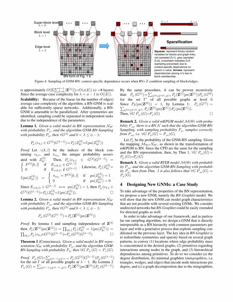
Sparsification

Squares: represent binary random variables for blocks and graph links; red (sampled Z=1), grey (sampled Z=0), crosshatch indicates Z=0 (sampling prevented) due to context-specific dependence on parent rv value. Arrows: represent dependencies among rv's due to block membership.

Z = 1 Z = 0

Z[1]j

Z[0]i

Auv

... ...

... ... ...

BN form of Fig. 1 b

Super-block level

Block level

Edge level� = 2

� = 1

� = 0

Figure 4: Sampling of GNM-BN: context-specific dependence occurs when RVs Z condition sampling of blocks/edges.

is approximately O(E[∑φ−1λ=0 |Z[λ]|])=O(φ|E|) (φ =# layers)

Since the average-case complexity for λ = φ− 1 is O(|E|).Scalability: Because of the linear (in the number of edges)average case complexity of the algorithm, a BN-GNM is scal-able for sufficiently sparse networks. Additionally, a BN-GNM is amenable to be parallelized. After symmetries areidentified, sampling could be separated in independent tasksdue to the independence of the parameters.Lemma 1. Given a valid model in BN representation NΘ′

with probability PN , and the algorithm GNM-BN-Samplingwith probability PS , then ∀G[λ] and 0 < λ ≤ φ− 1:

PN (ek,l ∈ G[λ]|G[λ−1])=PS (Z[λ]kl =1|pa(Z

[λ]kl ))

Proof. Let γ(k, l) be the indices of the block con-taining ek,l, and πσkl the unique probability associ-ated with Z

[λ]kl . Then, PN (ek,l ∈ G[λ]|G[λ−1]) ={

P [λ][k, l] if Eγ(k,l) ∈ G[λ−1]

0 if Eγ(k,l) /∈ G[λ−1] . Likewise, PS (Z[λ]kl =

1|pa(Z[λ]kl )) =

{πσkl = P [λ][k, l] if pa(Z

[λ]kl ) = 1

0 if pa(Z[λ]kl ) = 0

.

Since Eγ(k,l) ∈ G[λ−1] ⇐⇒ pa(Z[λ]kl ) = 1, then PN (ek,l ∈

G[λ]|G[λ−1])=PS (Z[λ]kl =1|pa(Z

[λ]kl )).

Lemma 2. Given a valid model in BN representation NΘ′

with probability PN , and the algorithm GNM-BN-Samplingwith probability PS , then ∀G[λ] and 0 < λ ≤ φ− 1:

PN (G[λ]|G[λ−1])=PS (Z[λ]|pa(Z[λ]))

Proof. By lemma 1 and sampling independence of Z[λ]

then PS (Z[λ]|pa(Z[λ])) =∏∀k,l PS (Z

[λ]kl = 1|pa(Z

[λ]kl )) =∏

∀k,l PN (ek,l∈G[λ]|G[λ−1])=PN (G[λ]|G[λ−1])

Theorem 1 (Correctness). Given a valid model in BN repre-sentation NΘ′ with probability PN , and the algorithm GNM-BN-Sampling with probability PS , then ∀G PN (G) = P

S(G).

Proof. PN (G)=∑G[λ−1]∈Γ[λ−1] PN (G[λ]|G[λ−1])PN (G[λ−1])

for the set Γ of all possible graphs at λ − 1. By Lemma 2PN (G) =

∑G[λ−1]∈Γ[λ−1],Z[λ] PS (Z[λ]|pa(Z[λ]))PN (G[λ−1])

By the same procedure, it can be proven recursivelythat: PN (G[1])=

∑G[0]∈Γ′[0],Z[1] PS (Z[1]|pa(Z[1]))PN (G[0])

for the set Γ′ of all possible graphs at level 0.Since PS(pa(Z[0])) = 1, by Lemma 1: PN (G[1]) =∑G[0]∈Γ′[0],Z[1] PS (Z[1]|pa(Z[1]))PS (pa(Z[1])).

Then, ∀G PN (G)=PS(G)

Remark 2. Given a valid mKPGM modelM(Θ) with proba-bility PM , there is a BN N such that the algorithm GNM-BN-Sampling, with sampling probability PS , samples correctlyfrom PM , i.e. ∀G PS (G) = PM(G).

Let PS be the probability of the GNM-BN sampling. Giventhe mapping MΘ r⇀NΘ′ , as shown in the transformation ofmKPGM to BN. Since the CPD are the same for the samplingand the BN representation, then, by Thm 1, ∀G PM(G) =PN (G)=PS (G)

Remark 3. Given a valid BTER modelM(Θ) with probabil-ity PM , and the algorithm GNM-BN-Sampling with probabil-ity PS , then from Thm. 1 it also follows that ∀G PM(G) =PS (G).

4 Designing New GNMs: a Case StudyTo take advantage of the properties of the BN representation,we propose a new GNM, namely the BN-Graphlet model. Wewill show that the new GNM can model graph characteristicsthat are not possible with several existing GNMs. We considerundirected networks but BN-Graphlet could be easily extendedfor directed graphs as well.

In order to take advantage of our framework, and in particu-lar our sampling algorithm, we design a GNM that is directlyinterpretable as a BN hierarchy with common parameters perlayer and with a generative process that exploits sampling con-ditioned on the previous layer. The key idea in BN-Graphlet isto redistribute symmetries and sparsity based on several graphpatterns, to convey (1) locations where edge probability massis concentrated in the desired graphs, (2) primitives regardinginteractions among nodes in the graph, and (3) hierarchicaldependencies among primitives. To do so we consider (a) thedegree distribution, (b) minimal graphlets (mingraphlets, i.e.triangles, wedges, and edges) that encode node interactions perdegree, and (c) a graph decomposition due to the mingraphlets.

The reason to use mingraphlets is that larger graphlets canbe constructed via algebraic transformations of the minimalgraphlets. Since each of these characteristics are dependenton the previous one, each will be encoded in a level of the BNhierarchy.

Let ∆ ∼ fdeg(θ∆) be the sequence of degrees drawn fromthe degree distribution fdeg. BN-Graphlet creates groups ofnδi nodes of degree δi for δi ∈ ∆. Then we can partitionthe adjacency matrix via the joint degree distribution, and useblock bij =B

[0]ij to refer to links among nodes with degrees

δi, δj respectively. Let P [0][i, j]=0 for blocks with no links;otherwise, P [0][i, j]=1.

Next, the model partitions a single block in sub-groups of nodes that link only triangles, only wedges,and the remainder, i.e., every block will be subdividedinto nine subblocks B[1]

·· . To simplify notation, we useB

[1]k=[1..3]l=[1..3](i, j) to refer to appropriate cell in B[1]

associated with its parent i, j in B[0]. Then: P [1][k, l] =p4bij

if k=1, l=1 i.e., both nodes link only to trianglesp∧bij if k=2, l=2 i.e., both nodes link only to wedges1 o.w.

Here p4bij and p∧bij are respectively: the probability that the

two nodes incident to an edge in block B[0]ij participate only in

triangles, and the probability that the two nodes incident to anedge in block B[0]

ij participate only in wedges.Lastly, the final adjacency matrix is constructed from sub-

matrices of size nδi × nδj for each degree pair δi, δj . Thenodes of each sub-matrix will be associated with roles basedon their parent B[1]

kl (i, j). For 3x3 submatrices of edges em,n,where m,n have the role only triangles, the off-diagonal edgeprobabilities in B[2]

mn will be all 1; for blocks where the nodeshave the role only wedges, there will be two edges with proba-bility 1s and one with probability 0. For all other edges, theprobability will be κ1/3

bij, where κbij is the clustering coeffi-

cient centered at a node in block B[0]ij .

It is straightforward to see that the BN N of BN-Graphletis directly derived from the blocks B[λ]

ij and their probabilities,contrary to mKPGM and BTER where transformations wereneeded. This is because we use our framework directly tobuild the GNM. The equivalence can be directly obtained withthe following procedure:

1. For λ = 0, . . . , 2

(a) For i, j = [1, rows(P [λ])], [1, cols(P [λ])]

i. Define Z [λ]ij the RV that models the blocks B[λ]

ij

ii. Define P (Z[λ]ij = 1|pa(Z

[λ]ij ) = 0) = 0

iii. Define P (Z[λ]ij =1|pa(Z

[λ]ij ) = 1) = P [λ][i, j]

Estimation: We need to estimate θ∆, the sequence κbij , andprobabilities p4bijand p∧bij. θ∆ is learned as the MLE of thefitted degree distribution. κbij is the clustering coefficient perblock of the data graph. The parameters p4bij and p∧bij areestimated as the MLE of the respective multinomial.

# of non isolated nodes# of non isolated nodes# of non isolated nodes

KPGM2⇥2 mKPGM ` = 6 BN-Graphlet

Avg. Clustering Coe�cientAvg. Clustering Coe�cient Avg. Clustering Coe�cient

Siz

eofLC

CA

vg.

Geo

des

icD

ista

nce

Siz

eofLC

C

Siz

eofLC

C

Avg.

Geo

des

icD

ista

nce

Avg.

Geo

des

icD

ista

nce

150 250 350 450 550

550

450

350

250

150

50

550

450

350

250

150

50

550

450

350

250

150

50

30

20

10

0

30

20

10

0

30

20

10

0 0.2 0.5 0.8 1 0.2 0.5 0.8 1 0.2 0.5 0.8 1

50 150 250 350 450 550

Figure 5: Variation of mKPGM and BN-Graphlet graph properties insynthetic networks. (LCC: largest connected component)

4.1 Experiments and AnalysisWe performed two sets of experiments. First, we encodedBN-Graphlet using the new representation and show, usingsynthetic networks, that it can model different networks com-pared to mKPGM. Because mKPGM was shown in [Morenoet al., 2013] to be capable of modeling a wider range ofnetwork characteristics than Chung Lu and KPGM models,in our experiments we compare to mKPGM. We generatednetworks for a wide range of parameter values Θ and plot-ted the characteristics of the sampled graphs. For mKPGM,we used 22,060 different values of Θ (b = 2). The pa-rameters were generated using every possible combinationof Θ, such that θ11, θ12 ∈ {0.01 : δ : 1.00}, θ12 = θ21,θ22 ∈ {θ11 : δ : 1}, and 2.1 ≤ ∑ij θij ≤ 2.4 We utilizedδ = 0.015 and θ12 ∈ {0.01 : δ : 1} to avoid repetitionof the parameters due to isomorphisms of Θ. For each Θsetting, we generated 75 undirected networks with mKPGM(K=9, `=6). For BN-Graphlet we considered θ∆ that leadto networks with a number of edges in the range [800, 2650]for a fair comparison with mKPGM models. For κbij wegenerated random values under the restriction that the globalclustering coefficient is realistic. The values of p4bijand p∧bijwere assigned using grid search.

We evaluate the characteristics of the generated networksusing: (1) average cluster coefficient, (2) average geodesicdistance, (3) number of non isolated nodes, and (4) size ofthe largest connected component. Figure 5 reports the results.BN-Graphlet produces the lowest geodesic distance (smallworld phenomena), the highest cluster coefficient (communitystructure), and largely reduces the number of isolated nodes(larger connected component). Thus BN-Graphlet can modelnetworks that are not easily modeled with mKPGM.

Second, we show that BN-Graphlet can model real worldnetworks better than the other models. We fitted the modelsto three real datasets: the CoRA citations network (comprises11,881 AI papers with 31,482 citations between them), the Na-tional Longitudinal Study of Adolescent Health (AddHealth)

0.2190.2250.159 0.127

0.936

0.113

0.345

0.668

0.213

0.859

0.261

0.388

0.00

0.25

0.50

0.75

1.00

AddHealth APhysics CoRA FacebookDatasets

KS

Dis

tanc

e

GNM BN−Graphlet mKPGM BTER

Figure 6: 3D-Kolgomorov-Smirnov distance across 4 datasets.

network (1155 nodes and 7884 edges), the astrophysics arXivnetwork (9,987 nodes and 25,973 edges), and Facebook wallpostings (449,748 nodes and 1,016,621 edges).

We compared the BN-Graphlet with BTER and mKPGM.Figure 6 shows the 3-dimensional Kolmogorov-Smirnov(KS

3D) distance of the learned to the true network charac-

teristics: hop-plot, degree, and clustering coefficient. In alldatasets, BN-Graphlet obtains the lowest error, except in Face-book where its error is the second lowest; showing it canjointly model the hop-plot, degree, and clustering coefficientof real networks consistently better than BTER or mKPGM.

5 Related Work and DiscussionGNMs have been developed in various ways, using differentmotivations and frameworks. There has been some work toidentify the common features of GNMs. For example, [Jacobsand Clauset, 2014] provides an overview of different familiesof GNMs and gives some important insights about relation-ships among them. [Rohe et al., 2011] considers the relationbetween the latent space model [Hoff et al., 2002] and stochas-tic block models [Holland et al., 1983]. However, these worksdo not consider complex GNMs with a hierarchical samplingprocess involving intermediate latent variables.

Previous work have used BNs to create GNMs [Schein etal., 2016; Liang et al., 2016; Ho et al., 2011; Neiswanger etal., 2014]. However, these works proposed a specific BN withthe purpose of solving a specific network problem (e.g., nodeactions, link predictions, etc). Our contribution is to proposea general representation that is not dependent on any dataset,problem, or BN topology, but rather only on an assumption ofconditional independence during sampling. Using this mini-mal building block, we have proposed a sampling method thatis universal across GNMs that fulfill this assumption.

Also related to our work is lifted inference. Lifted infer-ence algorithms identify and exploit abundant symmetries ingraphical models, in order to avoid repeated computationsand speed up probabilistic inference [Koller and Pfeffer, 1997;Poole, 2003; Jha et al., 2010; Van den Broeck and Darwiche,2013; Mittal et al., 2015; Sen et al., 2009]. Lifted ImportanceSampling (LIS) was proposed in relational learning for proba-bilistic inference [Gogate and Domingos, 2011], and extendedby [Gogate et al., 2012]. We note that their task is differentsince the symmetries are exploited to improve the precision ofLIS (i.e., reduce variance) while our work exploits parametricsymmetries for efficient network sampling, which providesguaranteed performance (both time complexity and correct-

ness) for GNMs. [Venugopal and Gogate, 2014] showed away to deal with situations where symmetries are broken. Asin their work, we show ways to find symmetries but in therealm of social network models.

In general, like these existing lifted-techniques, our liftedsampling identifies structural patterns in GNMs to sample aset of random variables as a group rather than treating eachrandom variable separately. This leads to an efficient and cor-rect sampling method. Unlike existing lifted-techniques, weuse symmetries to create a meta-model that encodes existingsocial network models and allows for creation of new ones.

In our work, we take advantage of the symmetries in theintrinsic graphical model of the GNMs for efficient samplingand then exploit the hierarchical representation to construct agenerative model that produces sampled graphs with character-istics that are not easily achieved with current GNM methods.In the experiments, we show the range of networks that can bemodeled with this new generative model. To our knowledge,our work is one of the first applications of lifted techniques thatexploits the symmetries existing in social network models.

6 ConclusionIn this paper, we showed how hierarchical GNMs that arespecified procedurally, can be represented as generally as BNs.Our unifying BN view provides the following advantages: (1)universal representation, which can highlight the similaritiesand differences between GNMs, and (2) efficient, provablycorrect and universal sampling, due to the adherence of thealgorithm to a directed BN structure and an efficient samplingalgorithm. The representation also facilitates the creation ofnew GNMs. To illustrate the benefits of the BN representationand associated sampling method, we proposed the hierarchicalBN-Graphlet model and showed it more accurately capturesthe structure of four real-world networks.

AcknowledgementsWe thank the anonymous reviewers for their useful comments.This research is supported by NSF under contract numbers:IIS-1546488, IIS-1618690, CCF-0939370, and by “CONI-CYT + PAI/Concurso nacional de apoyo al retorno de inves-tigadores/as desde el extranjero, convocatoria 2014 + folio82140043.”

References[Benson et al., 2014] Austin R. Benson, Carlos Riquelme,

and Sven Schmit. Learning multifractal structure in largenetworks. In Proceedings of the 20th ACM SIGKDD Inter-national Conference on KDD, 2014.

[Boutilier et al., 1996] Craig Boutilier, NirFriedman, MoisesGoldszmidt, and Daphne Koller. Context-specific indepen-dence in bayesian networks. In Proceedings of the 12thInternational Conference on UAI, pages 115–123, 1996.

[Chung and Lu, 2002] F. Chung and L. Lu. The averagedistances in random graphs with given expected degrees.PNAS, 99(25):15879–15882, 2002.

[Erdos and Renyi, 1960] P. Erdos and A. Renyi. On the evolu-tion of random graphs. In Publication of the MathematicalInstitute of the Hungarian Academy of Sciences, pages 17–61, 1960.

[Gogate and Domingos, 2011] Vibhav Gogate and Pedro M.Domingos. Probabilistic theorem proving. CoRR,abs/1202.3724, 2011.

[Gogate et al., 2012] Vibhav Gogate, Abhay Jha, and DeepakVenugopal. Advances in lifted importance sampling. InProceedings of the 26th AAAI Conference on Artificial In-telligence, pages 1910–1916, 2012.

[Ho et al., 2011] Qirong Ho, Ankur P. Parikh, Le Song, andEric P. Xing. Multiscale community blockmodel for net-work exploration. In AISTATS, 2011.

[Hoff et al., 2002] P. Hoff, A. Raftery, and M. Handcock. La-tent space approaches to social network analysis. Journal ofthe American Statistical Association, 97:1090–1098, 2002.

[Hoff, 2008] Peter D. Hoff. Multiplicative latent factor mod-els for description and prediction of social networks. Com-putational and Mathematical Organization Theory, 15(4),2008.

[Holland et al., 1983] Paul W. Holland, Kathryn BlackmondLaskey, and Samuel Leinhardt. Stochastic blockmodels:First steps. Social Networks, 5(2):109 – 137, 1983.

[Jacobs and Clauset, 2014] Abigail Z. Jacobs and AaronClauset. A unified view of generative models for networks:models, methods, opportunities, and challenges. In arXivstat, 2014.

[Jha et al., 2010] Abhay Jha, Vibhav Gogate, Alexandra Me-liou, and Dan Suciu. Lifted inference seen from the otherside : The tractable features. In Advances in NIPS. 2010.

[Kolda et al., 2014] Tamara G. Kolda, Ali Pinar, ToddPlantenga, and C. Seshadhri. A scalable generative graphmodel with community structure. SIAM Journal on Scien-tific Computing, 36(5):C424–C452, September 2014.

[Koller and Pfeffer, 1997] Daphne Koller and Avi Pfeffer.Object-oriented bayesian networks. In Proceedings of theThirteenth Conference on UAI, UAI’97, pages 302–313,San Francisco, CA, USA, 1997.

[Larremore et al., 2014] Daniel B. Larremore, Aaron Clauset,and Abigail Z. Jacobs. Efficiently inferring communitystructure in bipartite networks. Phys. Rev. E, 90:012805,Jul 2014.

[Leskovec et al., 2010] Jure Leskovec, DeepayanChakrabarti, Jon Kleinberg, Christos Faloutsos, andZoubin Ghahramani. Kronecker graphs: An approach tomodeling networks. JMLR, 11(Feb):985–1042, 2010.

[Liang et al., 2016] Dawen Liang, Laurent Charlin, JamesMcInerney, and David M. Blei. Modeling user exposure inrecommendation. In Proceedings of the 25th InternationalConference on World Wide Web, 2016.

[Mittal et al., 2015] Happy Mittal, Anuj Mahajan, Vibhav GGogate, and Parag Singla. Lifted inference rules with con-straints. In Advances in NIPS. 2015.

[Moreno et al., 2013] S. Moreno, J. Neville, and S. Kirsh-ner. Learning mixed Kronecker product graph models withsimulated method of moments. In 19th ACM SIGKDDInternational Conference on KDD, 2013.

[Moreno et al., 2014] S. Moreno, J. Pfeiffer III, S. Kirshner,and J. Neville. A scalable method for exact sampling fromKronecker family models. In IEEE 14th ICDM, Dec 2014.

[Neiswanger et al., 2014] W. Neiswanger, C. Wang, Q. Ho,and E. P. Xing. Modeling citation networks using latentrandom offsets. In Proceedings of 30th Conference on UAI,pages 485–492, 2014.

[Peixoto, 2014] Tiago P. Peixoto. Hierarchical block struc-tures and high-resolution model selection in large networks.Phys. Rev. X, 4:011047, Mar 2014.

[Pfeffer et al., 1999] Avi Pfeffer, Daphne Koller, Brian Milch,and Ken T. Takusagawa. Spook: A system for probabilisticobject-oriented knowledge representation. In Proceedingsof the 15th Conference on UAI, pages 541–550, 1999.

[Poole and Zhang, 2003] David Poole and Nevin LianwenZhang. Exploiting contextual independence in probabilisticinference. J. Artif. Intell. Res.(JAIR), 18:263–313, 2003.

[Poole, 2003] David Poole. First-order probabilistic infer-ence. In Proceedings of the 18th International Joint Con-ference on Artificial Intelligence, 2003.

[Rohe et al., 2011] Karl Rohe, Sourav Chatterjee, and BinYu. Spectral clustering and the high-dimensional stochasticblockmodel. Ann. Statist., 39(4):1878–1915, 08 2011.

[Schein et al., 2016] A. Schein, M. Zhou, D. M. Blei, andH. Wallach. Bayesian Poisson Tucker decomposition forlearning the structure of international relations. In ICML,2016.

[Sen et al., 2009] Prithviraj Sen, Amol Deshpande, and LiseGetoor. Bisimulation-based approximate lifted inference.In Proceedings of the 25th Conference on UAI, pages 496–505, Arlington, VA, United States, 2009.

[Seshadhri et al., 2012] C. Seshadhri, Tamara Kolda, and AliPinar. Community structure and scale-free collections ofErdos-Renyi graphs. Physical Review E, 85(5), 2012.

[Seshadhri et al., 2013] C. Seshadhri, Ali Pinar, and TamaraKolda. An in-depth analysis of stochastic Kronecker graphs.Journal of the ACM, 60(2), 2013.

[Van den Broeck and Darwiche, 2013] Guy Van den Broeckand Adnan Darwiche. On the complexity and approxima-tion of binary evidence in lifted inference. In Advances inNIPS, 2013.

[Venugopal and Gogate, 2014] Deepak Venugopal and Vib-hav Gogate. Evidence-based clustering for scalable infer-ence in markov logic. In Proceedings of ECML PKDD,pages 258–273, 2014.

[Yun and Vishwanathan, 2012] Hyokun Yun and S. V. N.Vishwanathan. Quilting stochastic kronecker productgraphs to generate multiplicative attribute graphs. In AIS-TATS, pages 1389–1397, 2012.