1

Unified Design Method for Flexure and Debonding in FRP Retrofitted RC Beams

G.X. Guan, Ph.D.1; and C.J. Burgoyne2

Abstract

Flexural retrofitting of reinforced concrete (RC) beams using fibre reinforced polymer (FRP)

plate is a common way to increase the flexural capacity. There is a lack of rational design

method to determine where the strengthening plate can safely be curtailed. As a result,

retrofitted beams commonly fail by debonding of the FRP plate, which occurs well before the

target flexural capacity. Debonding is brittle failure and thus ductility of the retrofitted beam

needs to be ensured by debonding prevention. With sufficient ductility the ultimate strength

can continuously increase beyond steel yields with the elastic behaviour of the FRP

strengthening plate. Debonding prevention has been accounted-for empirically in most

design approaches so far.

The Global Energy Balance Approach (GEBA) using fracture mechanics has been proposed

to determine the debonding load of an FRP-RC beam that is affected by the plate curtailment

location. The GEBA results for various FRP-RC beams can be summarised using debonding

contours on plots of moment capacity against the safe plate curtailment locations, and the

debonding contours constructed in this way for the beams with the same ratio of depth to

fracture energy are virtually the same. This paper shows how GEBA can be incorporated into

the design process to prevent premature debonding of the FRP plate. The method makes use

of the debonding contours and derives from these simplified design charts that could be made

available to designers. The retrofitting design consideration and the theoretical background of

this unified design method are first explained, followed by the derivation of the conceptual

design charts. Numerically correct design charts are then constructed for a wide range of

3

Introduction

FRP plate retrofitting considerations

FRP plates can be used to enhance the capacity of under-reinforced RC beams but has the

effect of reducing ductility. It is relatively easy to decide how much FRP is needed to

achieve a certain strength, but it is harder to ensure sufficient ductility and retrofitted beams

are known to suffer from premature debonding at loads below their design strength. This

paper shows how to design beams for strength, ductility and debonding prevention.

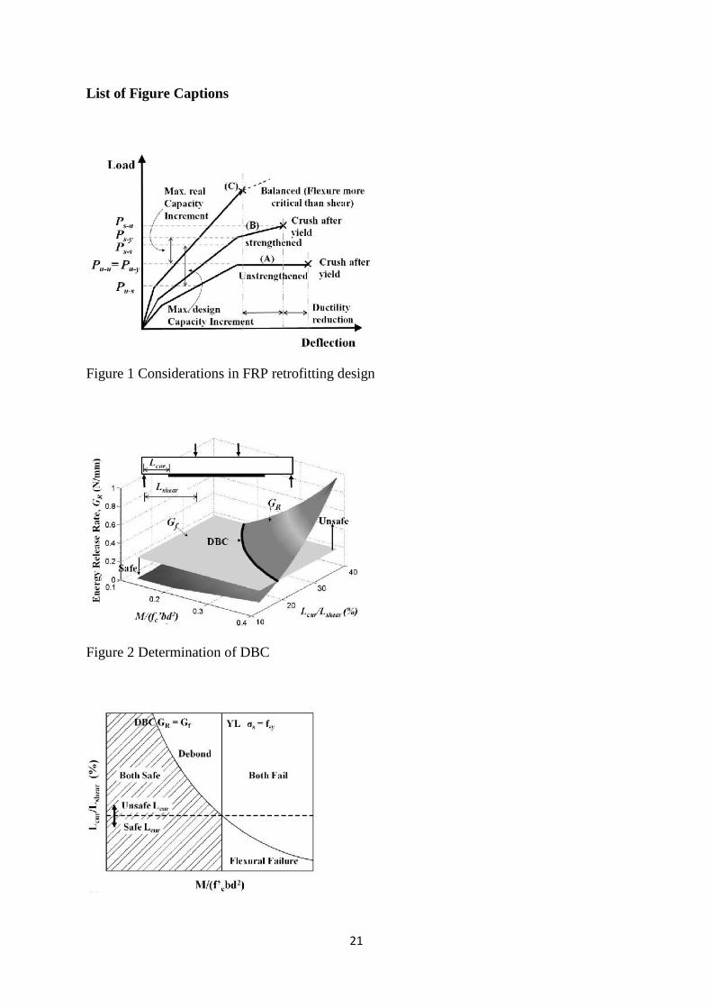
Figure 1 shows typical load deflection relationships for three beams. Curve (A) applies to an

unstrengthened under-reinforced beam; it has a relatively long plateau at virtually constant

load as the steel yields before the concrete crushes. Curve (B) shows the effect of adding a

moderate amount of strengthening; the beam yields at a higher load because of the presence

of the CFRP, and continues to resist more load after the steel yields because the CFRP

remains elastic. However, final crushing of the concrete occurs at a lower deflection because

the neutral axis is deeper. The limiting case is shown in Curve (C) for a balanced section,

where the concrete crushes at the same time as the steel yields.

The original service load is shown as Pu-s while the original ultimate load capacity is Pu-u.

There are several limits on the amount of flexural strengthening.

1. In order to prevent brittle failure, most RC beams are under-reinforced. Thus a beam

should not be over strengthened to become over-reinforced, so the corresponding

balanced section design limits the amount of FRP to be added (Curve C).

2. It is undesirable for the beam to undergo plastic deformation under normal service

loads to avoid accumulation of plastic deformation, so the retrofitted service load

limit (Ps-y) is calculated from the moment that causes first yield of the original steel

5

a place where the flexural strains are small. Strain criteria are thus not relevant. A study

based on fracture analysis of concrete, which relates the change in the strain energy in the

beam and the potential energy of the load to the energy that is released in the concrete when

the fracture propagates has been used to predict when debonding would occur. This is known

as the Global Energy Balance Approach (GEBA) (Achintha and Burgoyne 2008; Gunes et al.

2009; Carpinteri et al. 2009; Guan (2012); Guan and Burgoyne 2012). The key comparison

is between the Energy Release Rate GR with the Fracture Energy of Concrete Gf. The energy

release rate is calculated by comparing the energy difference per unit area for the same beam

under both presumed debonded and intact states with moment-curvature models for beam

energy estimate. The particular value that should be chosen for Gf will be discussed later but

is normally within the range 0.05 to 0.3 N/mm (Shah and Carpinteri 1991; Bazant and Becq-

Giraudon 2002).

A parametric study of GEBA has been presented by the authors in Guan (2012), where it is

shown that a debonding contour (DBC) plot can be used as the PE debonding criterion: GR

varies as a function of the loading state at which debonding occurs and as a function of where

the fracture takes place. GR is determined from M-κ models and the DBC can be plotted on a

graph of normalised moment capacity ( )'/( 2bdfM c ) against curtailment location

( shearcur LL / ), which allows the strength design and the debonding design to be combined, as

shown in Fig. 2.

The DBC is where the GR surface intercepts the horizontal plane that is defined by Gf. The

DBC varies for beams with different depths, reinforcing steel, FRP material etc. A detailed

discussion of the DBC is found in Guan (2012) where it was shown that a normalised

7

defines a limiting maximum curtailment length. If a beam is designed such that the beam

state point lies above this dashed line, premature debonding occurs before the beam’s flexural

capacity is reached.

It is axiomatic that the unstrengthened beam was under-reinforced, so debonding prevention

is going to depend heavily on the tension steel ratio ( s ) as well as the FRP ratio ( f ). To

strengthen a particular RC beam, s is fixed but the designer can change f , whereas when

considering the design of new beams s also varies. The effect of these two changes are

shown separately in Figs 4 (a) and (b); adding either type of reinforcement always moves YL

to the right (YL1 to YL2), but it has different effects on the DBC. Increasing f means that

debonding occurs more easily so the debonding line moves upwards. In contrast, with a

larger s , debonding is less likely so the debonding contour moves downwards. The

maximum curtailment (Lcur-max) changes correspondingly.

In order to make the above design charts cover a wide range of design cases, say for the

practical range for s from 0.4 to 2.0% and f from 0.1 to 1.5%, a very large number of

DBCs and YLs would be needed and the charts would be very complicated. However, it is

noted that the critical point is the intersection point of the DBC and YL. Any designed beam

state point below and to the left of this point is safe, which leads to the simpler design charts

described below. Two charts will be constructed; one for the pre-yielding stage which will be

shown to depend on the amount of steel, and the other will cover the post-yield condition and

will depend on the amount of FRP plate.

9

Although the service load must occur while the steel is still elastic, it has been noted above

that the beams may have to carry loads above yield in order to provide sufficient reserve of

strength. It is essential that the FRP does not debond before the ultimate strength of the beam

is reached. This can be accomplished by means of a different set of curves, which are

constructed in the same way as the STI curves, this time varying f only. The result is the

FRP-ratio track of intercepts (FTI) (Fig.6(a)).

As with the STI curves, one FTI curve replaces multiple DBCs. For any particular design,

the FTI line always lies below the DBC line once the applied moment exceeds the yield

moment (Fig 6(b)). Thus, using the FTI line to determine where the plate should be curtailed

is conservative for the post-yield condition. If the reserve of strength that is required beyond

yield is high, it is possible that a negative curtailment is predicted as shown in Fig.6(b) (no

positive intercept for the FTI at 1.5My). This indicates that an anchor is required in addition

to the bond.

Since increasing s makes debonding less likely while an increase of f makes it more likely,

the FTI and STI curves have a similar trend but different inclinations and for a particular

combination of ( s , f ) they cross each other at the yielding state.

Unified design procedures

It is now possible to produce a unified design procedure, making use of the STI and FTI

curves.

1. It is assumed that an existing beam is being strengthened, so the area of steel is known,

fixing s .

11

The charts given below are constructed for beams with cylindrical concrete strength fc’ =

37 MPa, with steel yield strength fy = 530 MPa and Young’s modulus Es = 200 GPa, and with

FRP elastic modulus Ef = 165 GPa. The STI and FTI are the locus of intersections of YLs

and DBCs. Here the YLs are constructed assuming the tension steel yields at the strain fy/Es,

the FRP plate behaves elastically, and the concrete in compression follows an unfactored

Hognestad-type parabolic stress-strain relationship (Hognestad et al. 1955). When

considering DBC, the most important parameter is the ratio h/Gf (MPa-1). It was shown in

Guan (2012) that DBCs for beams with the same h/Gf value are virtually identical. Thus the

DBCs and the resulting STI and FTI charts below apply to all the beams having the same

h/Gf .

Construction of detailed STI design charts

The STI curves can give a conservative design curtailment in the pre-yielding stage, so that

they are used to consider debonding prevention for the service state. Fig. 8(a) shows the

construction of a typical STI design chart that relates to a 400 mm deep beam, with Gf taken

as 0.15 N/mm, so h/Gf = 2.67×103 MPa-1. It has been produced by keeping f constant (at

0.5%) and varying s continuously. The family of thin curved lines are the DBCs for

different values of s , while the different vertical dashed lines are the corresponding YL lines.

The darker curved line is the STI which goes through the intersections of the corresponding

pairs of DBCs and YLs. The darker solid (vertical) line relates to ρs = 1.0%. One STI curve

covers the retrofitted design of a beam with a certain depth and f value, but various s values.

A similar set of curves is shown in Fig 8(b) for a beam of depth 800 mm and fracture energy

0.15 N/mm, so h/Gf = 5.3×103 MPa-1

13

Construction of detailed FTI design charts

The FTI curves can be constructed in a similar way. They give a conservative design

curtailment in the post-yielding stage and are thus adopted to ensure that debonding does not

occur up to the ultimate capacity. They are by keeping s constant and varying f

continuously. Figure 11(a) relates to a beam of 400 mm deep, with Gf taken as 0.15 N/mm; a

similar set of curves is shown in Fig 11(b) for a beam with depth of 800 mm.

By repeating the process for different s , a family of FTI is given to cover all the design

cases for 400 mm deep beams with h/Gf value as 2.67×103 MPa-1 (Fig 12).

As with the STI Band figures, the FTI Band figures are used to consider designs for beams

with the same h/Gf value but different depths. The FTI Band chart for h/Gf = 2.67×103 MPa-1

is as shown in Fig. 13, where the 1000 and 200 mm depth gives the left and right boundaries

respectively. The design procedure using FTI Band figures is the same as using STI Band

figures.

Significance of the simplified design

A pair of STI and FTI Band charts is required for one design to consider both service state

and ultimate state. Since h/Gf typically has a value in the range 0.5 – 20×103 MPa-1 for beams

ranging from 200 to 1000 mm deep, and having a Gf ranging from 0.05 to 0.30 N/mm, in

total, about ten pairs of STI and FTI Band charts are able to cover most design scenarios.

Thus, the simplified design with STI and FTI Band charts provides a convenient way for

practical engineering.

15

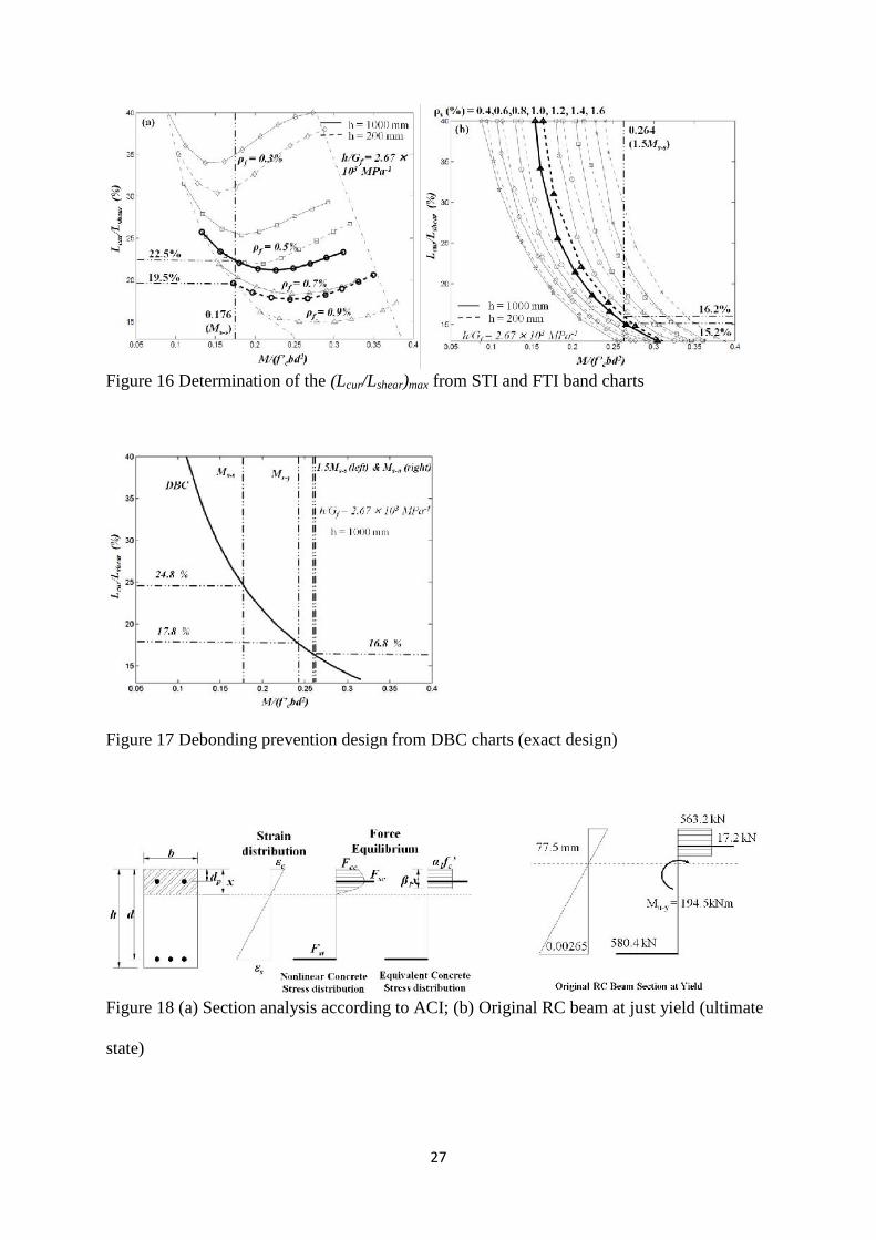
determines which sets of design charts to use is h/Gf , which is 400/0.15 = 2.67 MPa-1 in this

case. Fig. 16(a) is a reproduction of Fig. 10, but with the relevant lines highlighted. For the

service state, a vertical line is first drawn at M/(fc’bd2)= 0.176 which represents the moment

capacity required at service after retrofitting. Second, the maximum curtailments for beams

with depths of 200 mm and 1000 mm are given by its intersections with the STI curves at ρf =

0.7%, as Lcur/Lshear = 19.5% and 22.5% respectively. Then the maximum curtailment for the

400 mm beam in the problem is obtained from linear interpolation as Lcur/Lshear = 20.3%.

When considering the ultimate state, the FTI band charts are used for debonding prevention;

Figure 16(b) is a reproduction of Fig. 13, again with the relevant lines highlighted. Following

the same procedures, the maximum curtailment for the beam is estimated as

Lcur/Lshear = 16.0%. Consequently, the ultimate state governs the debonding prevention, and

the FRP plate should be curtailed less than 16.0% of the shear span away from the supports.

As explained in Sections 2 & 3 above, the curtailments predicted from the STI and FTI band

charts are conservative. The exact maximum curtailment obtained from DBC charts (exact

design) is also provided here (Fig. 17). The maximum values of Lcur/Lshear given by the exact

design at service and ultimate states are 24.8% (intercepting Ms-s) and 16.8% (intercepting

1.5Ms-s) respectively, which are greater than those predicted by simplified design above.

Furthermore, if the FRP plate is curtailed at 17.8% of the shear span, it debonds when the

tension steel yields. If the FPR plate is curtailed to 16.8%, debonding and crushing of

compressive concrete almost occur simultaneously, since in this case Mu-s (= 0.266) is close

to Ms-s (= 0.264). These values all exceed the value of 16.0% given by the simplified design

charts. It should be noted that the DBC curves would not generally be available to designers,

whereas it is suggested that simplified STI and FTI band charts could be provided.

17

This new method provides a way of incorporating a fracture mechanics approach to

debonding in a conventional beam design.

APPENDIX. Flexural capacity design for the beam in the worked example

STEP 1 Assessment of original capacity

The original design flexural capacity corresponds to the first yield of the section, as shown in

Fig. 18.

The concrete compression is calculated using an equivalent rectangular stress distribution

according to ACI318-08, where α1 and β1 are taken as 0.85 and 0.77 respectively, and the

results are in Fig. 18(b). From force equilibrium:

ysspsspc bdfbdEbxf '77.085.0 (1)

where 00265.0/ sys Ef ands

psp xd

dx

Substituting values and solving gives:

x = 77.5 mm; Fcc = 563.2 kN; Fsc = 17.2 kN; Fst = 580.4 kN.

Since the beam is under-reinforced, the contribution of the nominal compression steel is

negligible. The moment capacity of this unstrengthened section (at yield) is thus:

kNmxdFMM styuuu 5.419)5.7777.05.0365(4.580)77.05.0( (2)

STEP 2 Design of amount of strengthening

The beam is now to be strengthened so that Ms-s = 259.4 kNm, and Ms-u > 1.5 Ms-s so is

389.1 kNm. After some trial and error it is found that FRP plate having a cross-sectional area

equal to 0.7% of the beam section (ρf = 0.7%) will provide the necessary strengthening. This

amount of FRP is sufficient, by checking the new service and ultimate conditions, as shown

in Fig. 19.

19

Ps-s , Ps-y , Ps-u -- strengthened service/yield/ultimate load capacity

Pu-s , Pu-y , Pu-u -- unstrengthened service/yield/ultimate load capacity

tf -- Thickness of the FRP strengthening plate

ta -- Thickness of the adhesive layer

s -- Strain at tension steel

sp -- Strain at compression steel

f -- Strain at the centre of FRP strengthening plate

c -- Strain at top concrete fibre

s -- Tension steel ratio (As/(bd))

sp -- Compression steel ratio (Asp/(bd))

f -- FRP strengthening material ratio (Af/(bd))

-- Curvature

References

ACI Committee 440. (2008). Guide for the design and construction of externally bonded FRP

systems for strengthening concrete structures. Farmington Hills, MI, USA.

ACI Committee 318. (2008). Building code requirements for structural concrete and

commentary. Farmington Hills, MI, USA.

Achintha, P.M.M., and Burgoyne, C.J. (2008). “Fracture mechanics of plate debonding.” J.

Compos. Constr. 12(4):396-404.

Bazant, Z.P., and Becq-Giraudon, E. (2002). “Statistical prediction of fracture parameters of

concrete and implications for choice of testing standard.” Cem. Concr. Res. 32:529-56.

21

List of Figure Captions

Figure 1 Considerations in FRP retrofitting design

Figure 2 Determination of DBC

23

Figure 6 (a) Conceptual design chart with FTI (b) Comparison between FTI design and the

exact design

Figure 7 Comparison of the exact design, and design based on STI and FTI

Figure 8 (a) Construction of STI for beam having h = 400 mm and Gf = 0.15N/mm (b)

Construction of STI for beam having h = 800 mm and Gf = 0.15N/mm

25

Figure 11 (a) Construction of FTI for beam having h = 400 mm and Gf = 0.15N/mm (b)

Construction of FTI for beam having h = 800 mm and Gf = 0.15N/mm

Figure 12 Numerically correct FTI for 400 mm deep beam (h/Gf = 2.67×103 MPa-1)

27

Figure 16 Determination of the (Lcur/Lshear)max from STI and FTI band charts

Figure 17 Debonding prevention design from DBC charts (exact design)

Figure 18 (a) Section analysis according to ACI; (b) Original RC beam at just yield (ultimate

state)