Embed Size (px)
Citation preview

UNICORN: A BULK SYNCHRONOUSPROGRAMMING MODEL, FRAMEWORKAND RUNTIME FOR HYBRID CPU-GPU
CLUSTERS
TARUN BERI
DEPARTMENT OF COMPUTER SCIENCE ANDENGINEERING
INDIAN INSTITUTE OF TECHNOLOGY DELHI
MARCH 2016


UNICORN: A BULK SYNCHRONOUSPROGRAMMING MODEL, FRAMEWORKAND RUNTIME FOR HYBRID CPU-GPU
CLUSTERS
by
TARUN BERI
Department of Computer Science and Engineering
Submittedin fulfillment of the requirements of the degree of
Doctor of Philosophyto the
INDIAN INSTITUTE OF TECHNOLOGY DELHIMARCH 2016


Dedicated to my Family, Teachers and Friends ...


Certificate
This is to certify that the thesis titled Unicorn: A Bulk Synchronous Pro-
gramming Model, Framework and Runtime for Hybrid CPU-GPU
Clusters being submitted by Mr. Tarun Beri to the Indian Institute of
Technology Delhi for the award of the degree of Doctor of Philosophy in
Computer Science and Engineering is a record of original bonafide research work
carried out by him under our supervision. The work presented in this thesis has
reached the requisite standard and has not been submitted elsewhere either in
part or full for the award of any other degree or diploma.
Dr. Subodh Kumar
Associate Professor
Computer Science and Engineering
Indian Institute of Technology Delhi
Dr. Sorav Bansal
Assistant Professor
Computer Science and Engineering
Indian Institute of Technology Delhi


3
Acknowledgements
I always knew doing a Ph.D. from India's premier institute is tough and
along with a full time corporate job it was going to be even more so. I
am so grateful to my guide Prof. Subodh Kumar and co-guide Prof. Sorav
Bansal, who have understood my dual responsibilities at all times and made
this journey so smooth that today when I look back, it has actually been an
amazing experience. Today, I hold the highest regard for both of them and
I do not even have the slightest hesitation in recommending them as Ph.D.
guides to anyone. I am actually feeling uncomfortable of not being able to
put their invaluable contributions into appropriate words. Throughout the
duration of my Ph.D., their prudent advice and insightful knowledge have
been a constant source of inspiration and encouragement. Prof. Subodh’s
surprise visit to our paper presentation at IPDPS 2015 was quite reassuring
as well. I still remember the time when our paper faced a second consecutive
reject in a Tier 1 conference and both of them helped me sail through that
tough moment. To quote them “Many good papers get rejected 3 to 4 times
before they really rise to the top”. I am still learning a lot of things from
them and hope to replicate their formal writing skills one day.
My sincere thanks also goes to Prof. Kolin Paul, Prof. Preeti Panda and
Dr. Yogish Sabharwal who have been on the review committee for 5+ years
and have constantly provided invaluable guidance and feedback.
Working extremely hard and not stumbling to any challenge or work pressure
was infused in me right from my childhood. Being born to an influential and
highly educated joint family in a small town was a big boon. Somehow it

4
taught me to learn from each and every incident and person I came across.
My grandparents, parents, paternal and maternal uncles, cousins, in-laws and
their families were all instrumental in defining this success. When I was a kid,
everyone in my family especially my grand parents Mr. Nitrajan Pal Beri
and Mrs. Shakuntla Beri, my father Mr. Arun Beri and my uncles Mr. Anil
Beri and Mr. Raman Beri taught me for long hours and helped me build my
understanding on several basic concepts. My mother, Prof. Chander Beri,
who herself is a Ph.D. in mathematics, is the biggest motivation that has
driven me this far. It was her wish that I join this Ph.D. program and its
her confidence in me that I am now seeing its completion. Getting married
during the Ph.D. could have complicated things but my understanding and
supporting partner Tanvi and her parents Dr. Rajinder Mehta and Mrs.
Mala Mehta turned it into a delightful journey. Birth of my son, Taanish,
during this tenure proved to be the much needed rejuvenation. My brother
Ankur and his wife Ria also deserve a very special mention. Several of my
responsibilities often got offloaded to them while I was busy with my dual
work. Without any grief, they happily accepted this. God has also been very
kind to me.
Today, while writing this acknowledgement, I also recall all my school and
college teachers who have time and again instilled confidence in me and made
me believe in myself. I would also like to take this opportunity to thank my
long time friends Vineet Jindal, Jitesh Saghotra, Gurpreet Bedi, Amandeep
Bawa, Vikas Sarmal, Ajay Paul Singh, Amit Goyal, Gagan Bansal, Prateek
Prashar, Bikramjit Singh, Anand Sinha, Vijay Sharma, Asif Iqbal, Anish
Singla, Gaurav Gupta, Dilraj Singh, Thalinder Singh, Gagandeep Singh and

5
Narayan who have selflessly stayed along throughout.
My colleagues and friends at work Vineet Batra, Avinandan Sengupta, Ravi
Ahuja, Inderpal Bawa, Jatin Sasan, Harish Kumar, Tariq Rafiq, Sachin Pati-
dar, Rohil Sinha, Vaibhav Tyagi, Vikas Marda, Gordon Dow, Ahsan Jafri
and Pushp Agarwal also deserve a very special recognition for supporting me
helping me out directly or indirectly. While a few spared time to discuss
my project and share their feedback and new ideas, others helped me grasp
new technological advancements and learnings. I would also like to thank
the management of Adobe Systems India Pvt. Ltd. (Pankaj Mathur, Rajesh
Budhiraja, Lekhraj Sharma, Gaurav Jain and Viraj Chatterjee), Cadence De-
sign Systems India Pvt. Ltd. (Utpal Bhattacharya and Parag Chaudhary)
and STMicroelectronics India Pvt. Ltd. (Anand Singh and Vivek Sharma)
who have supported me and let me pursue my studies along with the office
work.
I would also like to thank M.Tech. students Harmeet Singh, Vigya Sharma,
Abhishek Raj, Abhishek Kumar and Ameen Mohammed who have worked
with me and helped develop the ideas in this work. In the end, my sincere
thanks goes to my mother’s friend and my teacher Mrs. Savita Sharma and
her husband Mr. Sunil Sharma who have always encouraged and supported
me since my childhood. I hope I shall make everyone proud in the time to
come and work even harder to take this work and knowledge to the next
level.
Tarun Beri

6

Abstract
Rapid evolution of graphics processing units (GPUs) into general purpose
computing devices has made them vital to high performance computing clus-
ters. These computing environments consist of multiple nodes connected by
a high speed network such as Infiniband, with each node comprising several
multi-core processors and several many-core accelerators. The difficulty of
programming hybrid CPU-GPU clusters often limits software’s exploitation
of full computational power. This thesis addresses this difficulty and presents
Unicorn – a novel parallel programming model for hybrid CPU-GPU clus-
ters and the design and implementation of its runtime.
In particular, this thesis proves that efficient distributed shared memory style
programing is possible. We also prove that the simplicity of shared memory
style programming can be retained across CPUs and GPUs in a cluster,
minus the frustration of dealing with race conditions. And this can be done
with a unified abstraction, avoiding much of the complication of dealing
with hybrid architectures. This is achieved with the help of transactional
semantics, deferred bulk data synchronization, subtask pipelining and various
communication and computation scheduling optimizations.
Unicorn provides a bulk synchronous programming model with a global ad-
dress space. It schedules concurrent tasks of a program in an architecture
and topology oblivious manner. It hides the network and exposes CPUs and
accelerators loosely as bulk synchronous computing units with logical phases,
respectively, of local computation and communication. Each task is further
decomposed into coarse-grained concurrently executable subtasks that Uni-
corn schedules transparently on to available CPU and GPU devices in the
cluster. Subtasks employ transactional memory semantics to access and syn-
chronize data, i.e., they check out a private view of the global shared memory

2
before their local computation phase and check in to the global shared mem-
ory afterwards, optionally resolving conflicting writes in a reduction step.
Unicorn’s main design goals are easy programmability and a deterministic
parallel execution environment. Device, node and cluster management are
completely handled by the runtime and no such API is exposed to the appli-
cation programmer. Load balancing, scheduling and scalability are also fully
transparent to the application code. Application programs do not change
from cluster to cluster to maintain efficiency. Rather, Unicorn adapts the
execution to the set of present devices, the network and their dynamic load.
Application code is oblivious to data placement within the cluster as well as
to changes in network interfaces and data availability pattern. Unicorn’s pro-
gramming model, being deterministic, eliminates data races and deadlocks.
To provide efficiency, Unicorn’s runtime employs several optimizations. These
include prefetching task data and pipelining subtasks in order to overlap their
communication with computations. Unicorn employs pipelining at two levels
– firstly to hide data transfer costs among cluster nodes and secondly to hide
DMA communication costs between CPUs and GPUs on all nodes. Among
other optimizations, Unicorn’s work-stealing based scheduler employs a two-
level victim selection technique to reduce the overhead of steal operations.
Further, it employs special proactive and aggressive stealing mechanism to
prevent the said pipelines from stalling (during a steal operation). To prevent
a subtask (running on a slow device or on a device behind a slow network or
I/O link) from becoming a bottleneck for the entire task, Unicorn reassesses
its scheduling decisions at runtime and schedules a duplicate instance of a
straggling subtask on a potentially faster device. Unicorn also employs a
software LRU cache at every GPU in the cluster to prevent the shared data
between subtasks getting DMA’ed more than once. To further boost GPU
performance, Unicorn makes aggressive use of CUDA streams and schedules
multiple subtasks for simultaneous execution.
To evaluate the design and implementation of Unicorn, we parallelize several
coarse-grained scientific workloads using Unicorn. We study the scalability

3
and performance of these benchmarks and also the response of Unicorn’s run-
time by putting it under stress tests like changing the input data availability
of these experiments. We also study the load balancing achieved in these
experiments and the amount of time the runtime spends in communications.
We find that parallelization of coarse-grained applications like matrix mul-
tiplication or 2D FFT using our system requires only about 30 lines of C
code to set up the runtime. The rest of the application code is regular single
CPU/GPU implementation. This indicates the ease of extending sequential
code to a parallel environment. The execution is efficient as well. Using
GPUs only, when multiplying two square matrices of size 65536∗65536, Uni-
corn achieves a peak performance of 7.81 TFlop/s when run over 28 Tesla
M2070 GPUs (1.03 TFlop/s theoretical peak) of our 14-node cluster (with
subtasks of size 4096 ∗ 4096). On the other hand, CUPLAPACK [28], a lin-
ear algebra package specifically coded and optimized from scratch, reports 8
TFlop/s while multiplying two square matrices of size 62000∗62000 using 32
Quadro FX 5800 GPUs (0.624 TFlop/s theoretical peak) of a 16 node cluster
connected via QDR InfiniBand.
Fine-grained applications, however, may not fit into our system as efficiently.
Such applications often require frequent communication of small data. This
is inherently against our bulk synchronous design and more advanced opti-
mizations may be needed to make these applications profitable.

4

Contents
1 Introduction 1
1.1 Application Model . . . . . . . . . . . . . . . . . . . . . . . . 3
1.2 Global Address Space . . . . . . . . . . . . . . . . . . . . . . . 4
1.3 Scheduling . . . . . . . . . . . . . . . . . . . . . . . . . . . . . 5
1.3.1 Reducing Steal Overhead . . . . . . . . . . . . . . . . . 7
1.3.2 Handling CPU-GPU Performance Disparity . . . . . . 7
1.4 Performance Optimizations . . . . . . . . . . . . . . . . . . . . 9
1.4.1 Data Transfer Optimizations . . . . . . . . . . . . . . . 10
1.4.1.1 Locality Aware Scheduling . . . . . . . . . . . 10
1.4.1.2 Pipelining . . . . . . . . . . . . . . . . . . . . 11
1.4.1.3 Grouping Communications . . . . . . . . . . . 11
1.4.1.4 Software GPU Caches . . . . . . . . . . . . . 12
1.4.2 Scheduling Optimizations . . . . . . . . . . . . . . . . 12
1.4.3 Address Space Optimizations . . . . . . . . . . . . . . 13
1.5 High Level Abstractions . . . . . . . . . . . . . . . . . . . . . 13
1.6 Epilogue . . . . . . . . . . . . . . . . . . . . . . . . . . . . . . 14
2 Programming Model 17
2.1 Data Subscriptions and Lazy Memory . . . . . . . . . . . . . . 23
6 CONTENTS
3 Runtime System 25
3.1 Device and Node Management . . . . . . . . . . . . . . . . . . 25
3.1.1 Runtime Internals . . . . . . . . . . . . . . . . . . . . . 27
3.1.2 List of Threads . . . . . . . . . . . . . . . . . . . . . . 31
3.2 Shared Address Spaces . . . . . . . . . . . . . . . . . . . . . . 32
3.3 Network Subsystem . . . . . . . . . . . . . . . . . . . . . . . . 41
3.4 Pipelining . . . . . . . . . . . . . . . . . . . . . . . . . . . . . 44
3.5 Scheduling Subsystem . . . . . . . . . . . . . . . . . . . . . . 45
3.5.1 Work Stealing in Unicorn . . . . . . . . . . . . . . . . 46
3.5.1.1 ProSteal . . . . . . . . . . . . . . . . . . . . . 49
3.5.1.2 Locality-aware Scheduling . . . . . . . . . . . 52
3.5.1.2.1 Greedy Scheduling . . . . . . . . . 54
3.5.1.2.2 Locality-aware work stealing . . . 55
3.5.2 Work-Group Calibration . . . . . . . . . . . . . . . . . 55
3.5.3 Multi-Assign . . . . . . . . . . . . . . . . . . . . . . . 57
3.5.3.1 Subtask Cancellation . . . . . . . . . . . . . . 58
3.5.4 Scheduling Across Task Barriers . . . . . . . . . . . . . 59
3.5.5 Scheduling Concurrent Tasks . . . . . . . . . . . . . . 60
3.6 Software GPU Cache . . . . . . . . . . . . . . . . . . . . . . . 60
3.7 Conflict Resolution . . . . . . . . . . . . . . . . . . . . . . . . 61
4 Pseudo Code Samples 65

CONTENTS 7
5 Experimental Evaluation 75
5.1 Unicorn Parallelization of Benchmarks . . . . . . . . . . . . . 78
5.1.1 Characteristics of Benchmarks . . . . . . . . . . . . . . 81
5.2 Performance Scaling . . . . . . . . . . . . . . . . . . . . . . . 82
5.2.1 CPU versus GPU versus CPU+GPU . . . . . . . . . . 85
5.2.2 PageRank . . . . . . . . . . . . . . . . . . . . . . . . . 88
5.3 Scheduling . . . . . . . . . . . . . . . . . . . . . . . . . . . . . 89
5.3.1 Work Stealing . . . . . . . . . . . . . . . . . . . . . . . 90
5.3.1.1 One-level vs. Two-level . . . . . . . . . . . . 91
5.3.1.2 ProSteal . . . . . . . . . . . . . . . . . . . . . 94
5.3.2 Locality-aware Scheduling . . . . . . . . . . . . . . . . 94
5.4 Load Balancing . . . . . . . . . . . . . . . . . . . . . . . . . . 100
5.5 Stress Tests . . . . . . . . . . . . . . . . . . . . . . . . . . . . 102
5.5.1 Heterogeneous Subtasks . . . . . . . . . . . . . . . . . 103
5.5.2 Input Data Distributions . . . . . . . . . . . . . . . . . 103
5.5.3 Varying Subtask Size . . . . . . . . . . . . . . . . . . . 104
5.6 Unicorn Optimizations . . . . . . . . . . . . . . . . . . . . . . 105
5.6.1 Multi-Assign . . . . . . . . . . . . . . . . . . . . . . . 106
5.6.2 Pipelining . . . . . . . . . . . . . . . . . . . . . . . . . 108
5.6.3 Software cache for GPUs . . . . . . . . . . . . . . . . . 109
5.6.4 Data Compression . . . . . . . . . . . . . . . . . . . . 110

8 CONTENTS
5.7 Overhead Analysis . . . . . . . . . . . . . . . . . . . . . . . . 111
5.7.1 Varying CPU cores . . . . . . . . . . . . . . . . . . . . 112
5.7.2 Unicorn Time versus Application Time . . . . . . . . . 114
5.7.3 Data Transfer Frequency . . . . . . . . . . . . . . . . . 115
5.8 Unicorn versus others . . . . . . . . . . . . . . . . . . . . . . . 116
6 Application Profiling 119
7 Public API 125
8 Related Work 145
9 Conclusions and Future Work 151
Bibliography 153
Appendix 163
10.1 Unicorn’s MapReduce Extension . . . . . . . . . . . . . . . . . 163
10.2 Scratch Buffers . . . . . . . . . . . . . . . . . . . . . . . . . . 164
10.3 Matrix Multiplication Source Code . . . . . . . . . . . . . . . 165
Unicorn Publications 175
Biography 177

List of Illustrations
Figures
2.1 Application program in Unicorn . . . . . . . . . . . . . . . . . 18
2.2 Mapping a BSP superstep to a Unicorn task . . . . . . . . . . 19
2.3 Execution Stages of a Subtask . . . . . . . . . . . . . . . . . . 20
2.4 Hierarchical Reduction - leaf nodes are subtasks, others are
reduced subtasks; dotted lines are inter-node data transfer . . 21
3.1 The design of the Unicorn runtime – Light orange region rep-
resents the instance of the runtime on each node in the cluster 27
3.2 Address Space Ownerships – PD represents Address Space
Ownership Directory, TD represents Temporary Ownership
Directory, x represents non-existent directory, red text repre-
sents changes from last state and cells in light blue background
represent directory changes via explicit ownership update mes-
sages; Node 1 is the address space master node. . . . . . . . . 37
3.3 Loss in victim’s pipeline due to work stealing . . . . . . . . . . 50
5.1 Characteristics of various benchmarks . . . . . . . . . . . . . . 82
5.2 Performance analysis of various benchmarks . . . . . . . . . . 83
5.3 Scaling with increasing problem size . . . . . . . . . . . . . . . 85
5.4 Image Convolution – GPU vs. CPU+GPU . . . . . . . . . . . 86

10 CONTENTS
5.5 Matrix Multiplication – GPU vs. CPU+GPU . . . . . . . . . 86
5.6 2D FFT – GPU vs. CPU+GPU . . . . . . . . . . . . . . . . . 87
5.7 Experiments with matrices of size 32768×32768 (lower is better) 88
5.8 Page Rank . . . . . . . . . . . . . . . . . . . . . . . . . . . . . 89
5.9 Centralized scheduling versus Unicorn – 14 nodes . . . . . . . 90
5.10 One-level versus two-level work stealing . . . . . . . . . . . . . 92
5.11 Work Stealing – with and without ProSteal . . . . . . . . . . . 93
5.12 Locality aware scheduling . . . . . . . . . . . . . . . . . . . . 96
5.13 Locality aware scheduling (Contd.) . . . . . . . . . . . . . . . 97
5.14 Image Convolution: Locality aware work-stealing (Derived Affin-
ity) . . . . . . . . . . . . . . . . . . . . . . . . . . . . . . . . . 99
5.15 Matrix Multiplication: Locality aware work-stealing (Derived
Affinity) . . . . . . . . . . . . . . . . . . . . . . . . . . . . . . 99
5.16 Load Balancing (Image Convolution) – W denotes a CPU work
group and G denotes a GPU device – Block random data dis-
tribution . . . . . . . . . . . . . . . . . . . . . . . . . . . . . . 101
5.17 Load Balancing (Page Rank) – W denotes a CPU work group
and G denotes a GPU device . . . . . . . . . . . . . . . . . . . 102
5.18 Load Balancing (Matrix Multiplication) – 32768× 32768 ma-
trices – Centralized data distribution . . . . . . . . . . . . . . 102
5.19 Load Balancing (Heterogeneous Subtasks) – W denotes a CPU
work group and G denotes a GPU device . . . . . . . . . . . . 103
5.20 Impact of initial data distribution pattern . . . . . . . . . . . 104

CONTENTS 11
5.21 Subtask size (N ×N) – experiments executed on 14 nodes . . 105
5.22 Multi-Assign (no external load) . . . . . . . . . . . . . . . . . 106
5.23 Multi-assign under external load (Image Convolution) – 4 nodes106
5.24 Pipelining (Image Convolution) . . . . . . . . . . . . . . . . . 108
5.25 Matrix Multiplication – GPU Cache Eviction Strategies . . . . 109
5.26 PageRank data compression (250 million web pages) . . . . . 111
5.27 Varying CPU cores used in subtask computation . . . . . . . . 112
5.28 Matrix Multiplication – Varying CPU core affinity . . . . . . . 113
5.29 Library time versus application time . . . . . . . . . . . . . . 114
5.30 Data Transfer Frequency . . . . . . . . . . . . . . . . . . . . . 115
5.31 Unicorn versus StarPU . . . . . . . . . . . . . . . . . . . . . . 117
5.32 Unicorn versus SUMMA . . . . . . . . . . . . . . . . . . . . . 117
6.1 Sample Unicorn Logs (part 1) . . . . . . . . . . . . . . . . . . 119
6.2 Sample Unicorn Logs (part 2) . . . . . . . . . . . . . . . . . . 120
6.3 Sample Unicorn Logs (part 3) . . . . . . . . . . . . . . . . . . 121
6.4 Performance . . . . . . . . . . . . . . . . . . . . . . . . . . . . 123
6.5 Load Balance . . . . . . . . . . . . . . . . . . . . . . . . . . . 123
6.6 Compute Communication Overlap . . . . . . . . . . . . . . . . 124
6.7 Event Timeline . . . . . . . . . . . . . . . . . . . . . . . . . . 124
Codes
4.1 Unicorn program for square matrix multiplication . . . . . . . 66
4.2 Unicorn callbacks for square matrix multiplication . . . . . . . 68
4.3 Unicorn program for 2D-FFT . . . . . . . . . . . . . . . . . . 70
4.4 Unicorn callbacks for 2D-FFT . . . . . . . . . . . . . . . . . . 72
7.1 Unicorn Header: pmPublicDefinitions.h . . . . . . . . . . . . . 125
7.2 Unicorn Header: pmPublicUtilities.h . . . . . . . . . . . . . . 142
10.1 File matmul.h . . . . . . . . . . . . . . . . . . . . . . . . . . . 165
10.2 File matmul.cpp . . . . . . . . . . . . . . . . . . . . . . . . . . 166
10.3 File matmul.cu . . . . . . . . . . . . . . . . . . . . . . . . . . 172

Chapter 1
Introduction
High performance computing environments consist of multiple nodes con-
nected by a network. Each node may comprise multi-core processors (CPUs)
and possibly many-core accelerators like graphics processing units (GPUs).
Attractive performance per-$ and per-watt of such accelerators have rendered
them mainstream in scientific and other domains. Nonetheless, writing effi-
cient programs employing both CPUs and GPUs across a network remains
challenging.
Traditionally, two major parallel programming paradigms have been pro-
posed – the first is a shared memory approach while the second is based
upon message passing. Shared memory programming [19] is considered in-
tuitive and familiar, but it quickly becomes inefficient as the shared memory
gets distributed (DSM) across a network [45, 3, 49, 52]. This is because DSM
systems generally employ complex memory consistency protocols (often re-
quiring application specific knowledge) resulting in high coherence overheads.
On the other hand, message passing alternatives like MPI [36] generally re-
quire transfer of not only data but also some control and program state in-
formation. With a large number of small data transfers, the latency quickly
becomes a bottleneck. Also, maintaining the additional baggage of control
and state information complicates MPI programs.
Our system uses the best of these two worlds by exposing a DSM style model

2 Introduction
to the programmer but behind the scenes employs shared memory (within
a node) and message passing (across nodes) for data transfers. Deferred
data exchanges in bulk amortize message passing overheads. Bulk synchro-
nization also eliminates race conditions and provides determinism, signifi-
cantly simplifying programming effort. Our work concludes that efficiency
can indeed be achieved with bulk-synchronous distributed shared memory.
In particular, we demonstrate that the traditional inefficiency of the shared
memory approach can be offset by hiding communication latency behind
coarse-grained computation and batching communication using ideas from
transactional memory: the application operates on local views of the global
shared memory and inter-view conflict is resolved lazily.
GPUs are discrete off-chip devices with exclusive memory and user must of-
ten explicitly copy the data from the host CPU. Once data is copied to the
device, the GPU works independently and after finishing the computation,
the user synchronizes the results back into the host memory. The explicit
placement and retrieval of data in GPU memory and the SIMD execution
of thousands of hardware threads in lock-step makes GPU programming a
lot more complex than traditional CPU programming. As such, it is desir-
able not to further complicate this when designing programming models for
GPU clusters. Our choice of abstracting the simplicity of distributed shared
memory style programming is a step in that direction.
Our programming model is based on the theoretical Bulk Synchronous Par-
allel computing model (BSP) [57] and thus complete. This thesis belies the
conventional wisdom that BSP is only a bridging model and too inefficient to
act as a real programming model. The thesis shows that with balanced load
1.1 Application Model 3
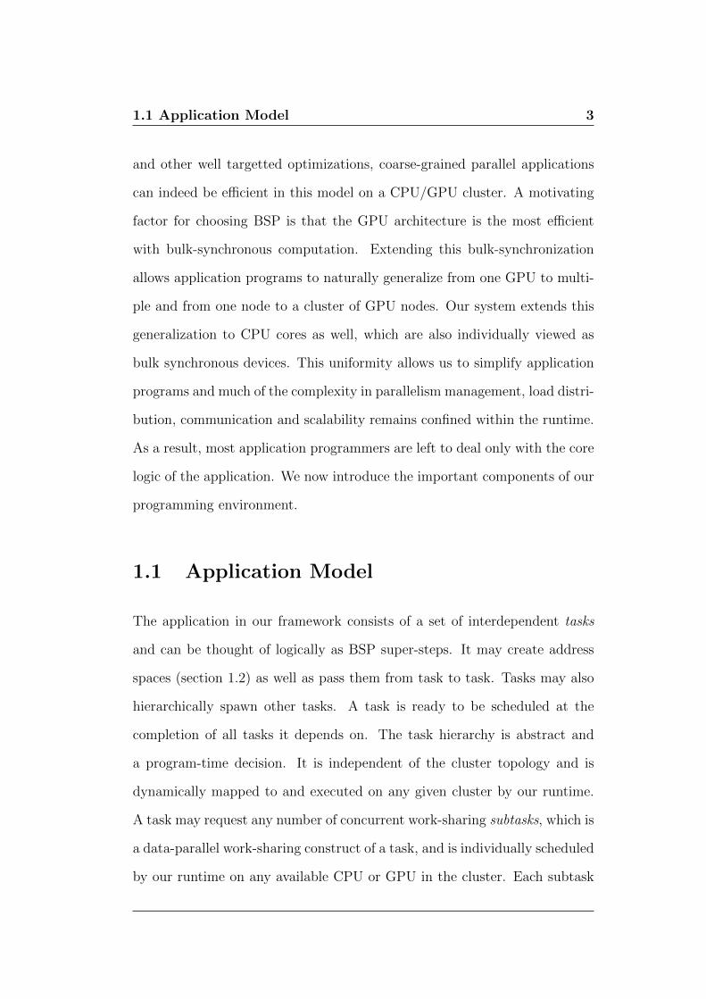
and other well targetted optimizations, coarse-grained parallel applications
can indeed be efficient in this model on a CPU/GPU cluster. A motivating
factor for choosing BSP is that the GPU architecture is the most efficient
with bulk-synchronous computation. Extending this bulk-synchronization
allows application programs to naturally generalize from one GPU to multi-
ple and from one node to a cluster of GPU nodes. Our system extends this
generalization to CPU cores as well, which are also individually viewed as
bulk synchronous devices. This uniformity allows us to simplify application
programs and much of the complexity in parallelism management, load distri-
bution, communication and scalability remains confined within the runtime.
As a result, most application programmers are left to deal only with the core
logic of the application. We now introduce the important components of our
programming environment.
1.1 Application Model
The application in our framework consists of a set of interdependent tasks
and can be thought of logically as BSP super-steps. It may create address
spaces (section 1.2) as well as pass them from task to task. Tasks may also
hierarchically spawn other tasks. A task is ready to be scheduled at the
completion of all tasks it depends on. The task hierarchy is abstract and
a program-time decision. It is independent of the cluster topology and is
dynamically mapped to and executed on any given cluster by our runtime.
A task may request any number of concurrent work-sharing subtasks, which is
a data-parallel work-sharing construct of a task, and is individually scheduled
by our runtime on any available CPU or GPU in the cluster. Each subtask

4 Introduction
executes an application-provided “kernel function,” which must determine
its share of work based on its subtask id and any task-wide parameters.
Unicorn schedules subtasks on devices (CPU or GPU), in a load-balanced
manner while also accounting for the location of their data.
Unlike many other distributed programming models (section 8), we do not
expect our applications to provide a dependency graph comprising all schedu-
lable entities (subtasks in our case). Rather, Unicorn based applications
specify dependencies only among tasks. These dependencies are implicit and
inferred by Unicorn from associated address spaces and their specified usage
(read-only, write-only, read-write). Subtasks of a task are concurrent with
no inter-dependencies. This has two advantages. First, it is natural to think
of an application as a graph of tasks (as opposed to a graph of subtasks).
Second, this reduces the size and processing time of dependency graph and
lets us perform several optimizations among subtasks. These optimizations
include out-of-order subtask execution, arbitrary grouping of subtasks, freely
migrating subtasks across cluster nodes, etc.
1.2 Global Address Space
Our runtime supports allocation of global shared memory regions called ad-
dress spaces. Usually a task’s input and output are stored here. While an
address space is logically shared, it may be physically distributed across mul-
tiple machines and devices by our runtime. The task registers callbacks to
indicate input data distribution and access patterns, the subtask logic and
the logic to combine, i.e., reduce, subtask-local output into the shared space.
1.3 Scheduling 5
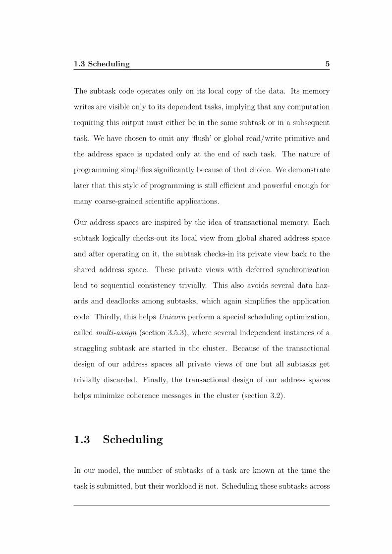
The subtask code operates only on its local copy of the data. Its memory
writes are visible only to its dependent tasks, implying that any computation
requiring this output must either be in the same subtask or in a subsequent
task. We have chosen to omit any ‘flush’ or global read/write primitive and
the address space is updated only at the end of each task. The nature of
programming simplifies significantly because of that choice. We demonstrate
later that this style of programming is still efficient and powerful enough for
many coarse-grained scientific applications.
Our address spaces are inspired by the idea of transactional memory. Each
subtask logically checks-out its local view from global shared address space
and after operating on it, the subtask checks-in its private view back to the
shared address space. These private views with deferred synchronization
lead to sequential consistency trivially. This also avoids several data haz-
ards and deadlocks among subtasks, which again simplifies the application
code. Thirdly, this helps Unicorn perform a special scheduling optimization,
called multi-assign (section 3.5.3), where several independent instances of a
straggling subtask are started in the cluster. Because of the transactional
design of our address spaces all private views of one but all subtasks get
trivially discarded. Finally, the transactional design of our address spaces
helps minimize coherence messages in the cluster (section 3.2).
1.3 Scheduling
In our model, the number of subtasks of a task are known at the time the
task is submitted, but their workload is not. Scheduling these subtasks across

6 Introduction
the cluster with balanced load is an important ingredient to scalable compu-
tation. Broadly, two dynamic load balancing strategies have been proposed
in the past – Push and Pull. In the former, overloaded computing devices
send work to others while in the latter, underloaded devices ask for work
from others. Push schemes are generally used for small centralized systems
as they do not scale well on larger ones. For de-centralized systems, Pull
schemes offer better scalability and fault tolerance. Work stealing is one
of the most effective examples of Pull based dynamic load balancing and
has been employed in many language and library based systems like Mul-T
[46], Cilk [14], OpenMP [19], Intel’s Thread Building Blocks (TBB) [56] and
Microsoft’s Parallel Patterns Library (PPL) [16].
Although work stealing (with random victim selection) has proven to be
quite effective in several parallel systems, it poses several challenges in our
context of hybrid CPU-GPU clusters. First, care is needed to limit the
overhead of stealing. This is particularly true in the context of task pipelines,
where a given subtask flows through many stages like input preparation stage,
data fetch stage, execution stage, etc. Sometimes it is useful to steal a
subtask before a computing device exhausts its pipeline, but it is also more
complicated. Secondly, the effectiveness of work-stealing tends to reduce as
the heterogeneity and computational disparity between devices grows. CPUs
allow threads to be scheduled on a single core, but GPUs do not allow per-core
scheduling and kernels can occupy the entire GPU. Subtasks large enough
to effectively use the GPU can be too slow on the CPU. Shorter ones may
improve CPU performance, but GPUs remain under-utilized. This disparity
between CPUs and GPUs poses scheduling challenges.

1.3 Scheduling 7
1.3.1 Reducing Steal Overhead
Unicorn uses two techniques to limit the overhead of stealing. First, it em-
ploys a steal-agent per node in the cluster. Due to shared memory usage,
the agent is able to easily monitor local load and track the ability of each lo-
cal device to service an incoming steal request. This guided victim selection
helps making more targeted steal requests, thereby reducing the number of
unsuccessful steal attempts in the cluster. The selection of a victim node for
a steal request remains random.
Secondly, Unicorn employs a proactive stealing technique called ProSteal.
When a device runs out of work (i.e., subtasks), its task pipeline stalls. It can
no longer overlap communication of subtasks with computation of others. It
needs to prime its task pipeline afresh after it steals a new subtask. Unicorn
prevents this performance loss in the system by stealing early (especially
for GPU devices) with one or more subtasks still pending with the device.
The exact number of subtasks pending with a device at the time of steal is
computed dynamically based on the device’s rate of subtask execution and
the observed latency to prime the pipeline after a stall (section 3.5.1.1).
1.3.2 Handling CPU-GPU Performance Disparity
Task decomposition in our system remains in user’s control. However, this
can sometimes be tedious. Unicorn simplifies application’s subtask sizing by
adjusting it to suit the current execution environment. However, choosing
sizes for heterogenous devices in the presence of high diversity is tricky.
One alternative, to address the CPU-GPU performance disparity, is to let
8 Introduction
the application programmer design subtasks differently for different devices.
But this would compromise abstraction and simplicity of programming. In
our framework, applications logically partition tasks and remain unaware of
where each subtask is scheduled. In any case, dynamically adapting subtask
sizes to the current execution environment can be a tedious exercise for the
application programmer.
Another alternative is to group, say, multiple CPU cores together into a
single device, but this can become complicated with a large number of device
types with diverse capabilities. Additionally, this would also compromise
the simplicity of the programming model as each kernel must execute on a
“set of devices.” This also takes away the liberty to use existing sequential
CPU functions as subtask kernels, an important design goal for us. Another
alternative is to envision a subtask as a set of work-items and schedule a
single work-item per CPU core. This is analogous to OpenCL’s [55] work-
group and work-item. This feature is implemented in our system but again
tasks may opt to disregard it in the interest of simplicity. However, in that
case all CPU cores and GPUs uniformly execute the subtasks of the same
size.
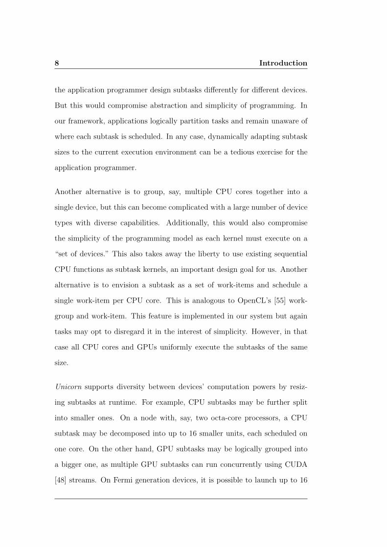
Unicorn supports diversity between devices’ computation powers by resiz-
ing subtasks at runtime. For example, CPU subtasks may be further split
into smaller ones. On a node with, say, two octa-core processors, a CPU
subtask may be decomposed into up to 16 smaller units, each scheduled on
one core. On the other hand, GPU subtasks may be logically grouped into
a bigger one, as multiple GPU subtasks can run concurrently using CUDA
[48] streams. On Fermi generation devices, it is possible to launch up to 16

1.4 Performance Optimizations 9
subtasks simultaneously. This example allows a skew of 1:256 in the size of
the subtasks executed on CPUs versus those executed on GPUs. Results in
section 5.5.3 show the performance improvement obtained by creating such
skew on a variety of subtasks.
In general, an application should empirically determine an appropriate sub-
task size. The goal here is not to select a subtask size that causes too many
CPU cache misses or keeps the GPU largely under utilized. Experimenting
with a small data set exclusively on one GPU and exclusively on one CPU
should help in making this decision.
1.4 Performance Optimizations
Besides the two work-stealing optimizations mentioned above, Unicorn em-
ploys several other optimizations for efficiency. Some of these performance
optimizations target scheduling while others focus on data transfers and min-
imizing control messages within the runtime. The optimizations include:
1. Data affinity based subtask scheduling to reduce data transfers within
the cluster
2. Pipelining subtask data transfers and computation in order to hide
communication latency
3. Grouping communications among a pair of nodes to reduce network
latency
4. Software cache in GPUs to boost re-use of shared read-only data among
subtasks

10 Introduction
5. Scheduling multiple instances of the same subtask in the cluster to
prevent stragglers
6. Spatially optimized address space accesses
7. Lazy address space coherence within the runtime to reduce manage-
ment messages
We briefly introduce the main optimizations next.
1.4.1 Data Transfer Optimizations
Some of data transfer optimizations explicitly focus on reducing the amount
of data transferred in the cluster, while others attempt to reduce the data
transfer time by hiding it behind other ongoing useful computation.
1.4.1.1 Locality Aware Scheduling
Often a coarse-grained computation is decomposed such that adjacent sub-
tasks exhibit spatial locality and access adjacent regions of input address
spaces. However, this is sometimes infeasible or it is overly complicated to
write programs in this fashion. To help such application programs, our run-
time maintains a distributed map of data resident on various nodes and uses
it to estimate the affinity of work to different nodes to guide scheduling.
Traditionally, locality-aware scheduling has mostly focussed on maximizing
reuse of resident data. This approach tends to schedule computation (or
subtasks) on nodes having the largest amount of input data resident. We,
however, observe that it is equally important to focus on minimizing the cost

1.4 Performance Optimizations 11
of fetching the non-resident data because significant time can be lost in fetch-
ing remote data and different devices are able to consume data at different
rates. Thus, our locality-aware scheduler takes into account the time spent
in fetching remote data and strives to minimize it.
1.4.1.2 Pipelining
To further reduce the cost of fetching remote data, Unicorn anticipates sub-
tasks a device may run in the future and fetches its data, hiding communi-
cation latency behind ongoing computation. Our scheduler makes subtask
assignments in groups. Subtasks in the group are sequentially executed start-
ing with the first one. While a device is executing the first subtask in the
assigned group, the next subtask overlaps its communication with the ongo-
ing computation of the first subtask. Similarly, the third subtask overlaps its
communication with the second subtask’s computation. This continues for
all subsequent subtasks in the group.
This mechanism is especially useful for GPUs capable of compute-communication
overlap and multiple kernel launches, where we create a pipeline of subtasks.
At any given time, one subtask may be transferring its data to the GPU, one
or more subtasks may be executing and one subtask may be copying its data
out of the GPU.
1.4.1.3 Grouping Communications
Often subtasks access data in patterns. This is especially true of regular
coarse-grained experiments where a subtask may access multiple contiguous
ranges of data with uniform separation. In such cases, our runtime detects the

12 Introduction
access pattern and instead of issuing multiple remote data transfer requests
for each subtask, one unified request is issued. At the remote end, the data is
packed before being sent to the requestor where it is unpacked and mapped
into the requesting subtask’s local view. This optimization helps scalability
as it prevents flooding of the network with too many small data transfer
requests. This also simplifies application programs, which do not need to
consider data and communication granularity.
1.4.1.4 Software GPU Caches
In addition to on-CPU caches of memory fetched from remote nodes, our
runtime system maintains an on-GPU software LRU cache for portions of
the address spaces currently loaded on the GPU device. This greatly helps
eliminate unnecessary data transfers when the same read-only data is re-
quested by multiple subtasks scheduled on that GPU, or in cases where data
written by a subtask is later read by another subtask of a subsequent task.
1.4.2 Scheduling Optimizations
Among the scheduling optimizations, Unicorn employs special mechanism to
prevent a few straggling subtasks from becoming a bottleneck for the entire
application. If a subtask executing on a device in the cluster takes long to
finish, while other devices have become idle, Unicorn’s scheduler may multi-
assign, i.e., assign the same subtask to multiple devices. We never migrate
away the subtask from the “slow” unit, allowing the multi-assigned units
to compete. Migration overheads are high and unnecessary: multi-assign
happens only near the end of a task. The results of the first finishing device

1.5 High Level Abstractions 13
are employed and the unused subtasks are aborted and their local writes are
discarded. This optimization also helps tackle situations where a subtask
straggles as a result of a slow network link or excessive load on one or more
nodes in the cluster.
1.4.3 Address Space Optimizations
Unicorn’s address spaces are specifically designed for efficient transactional
semantics and to minimize explicit cache coherence messages. We do not em-
ploy the usual MSI coherence protocol as it has the potential to generate too
many cache invalidations. The transactional semantics mean that a subtask
sees the global data at the beginning of the task, and then only its own up-
dates to that data. After the task finishes, the writes of the subtasks become
visible to subsequent tasks. Thus, we need no explicit coherence messages
during the task execution. Only at the end of the task, a few coherence
messages may be exchanged to invalidate outdated copies of data.
Address spaces are also optimized for linear and block accesses. Subtasks
needing one or more contiguous data ranges (like elements of an array) may
request for optimized linear accesses while subtasks needing one or more
uniformly separated contiguous data ranges (like sub-matrix of a bigger ma-
trix) may request for optimized block accesses. Internally, Unicorn organizes
address spaces to adapt to the kind of requested access.
1.5 High Level Abstractions
Unicorn is an extensible framework and it is possible to optimally orchestrate

14 Introduction
its functionality into other well known programming models like Map-Reduce
[20]. Chapter 2 describes the set of supported callbacks in Unicorn. The Sub-
task Execution callback can serve as the Map stage whereas the Data Syn-
chronization callback can be programmed to synchronize subtasks reducing
two a time. Chapter 5 evaluates this approach by implementing page-rank
[51] computation for a collection of web pages. The map stage of the ex-
periment computes contributions of PageRank for all outlinks in the web.
The reduce stage accumulates individual contributions on all inlinks for each
webpage. Results demonstrate the efficiency of Unicorn’s implementation
and its Map-Reduce suitability in general.
1.6 Epilogue
In addition to demonstrating the efficacy of the proposed system, this thesis
explores various optimization parameters. For pipelining, we explore when to
allow steal and study the impact of pipeline-flush. We explore various GPU
cache policies and the impact of application-provided hints. We study when to
multi-assign and how often the later assigned device finishes first. We analyze
the impact of variance in application controlled subtask size. We also study
the impact of changing input data availability patterns in the cluster. The
primary contributions of this work are:
1. We present a novel shared-memory based parallel programming model
that transparently maps and autonomously schedules computation on
any cluster of CPUs and GPUs in a load-balanced fashion.

1.6 Epilogue 15
2. We develop a runtime framework supporting the proposed model and
investigate the optimizations necessary for such a framework to be prac-
tical. Our runtime (Unicorn) batches and combines data transfer for
efficient communication. It performs prefetching and pipelining allow-
ing compute-communication overlap. It also supports multi-scheduling
in response to dynamically changing load.
3. We present a concrete study of scheduling in hybrid CPU-GPU clus-
ters. Specifically, we propose ProSteal which is a proactive and aggres-
sive stealing approach that avoids GPU pipeline stalls. We also explore
locality aware scheduling for subtasks written in no particular order of
spatial locality. We also present a technique to dynamically group sub-
tasks on GPU and split subtasks among CPU cores, effectively support-
ing a large variation in subtask sizes for efficient execution on devices
of variable computing power.
The rest of the thesis is organized as follows. Chapter 2 provides more insights
into the Unicorn’s programming model. Chapter 3 describes Unicorn’s run-
time and internal implementation details at length. Chapter 4 discusses the
pseudo-code implementation of matrix multiplication and two dimensional
Fast Fourier Transform experiments in our system. Chapter 5 discusses the
parallelizations of a few scientific benchmarks on Unicorn. The chapter also
evaluates the performance of these benchmarks along with an overhead and
stress analysis of our runtime. Chapter 6 discusses Unicorn’s application
profiling tool. Chapter 7 provide a reference to Unicorn’s public header files.
Chapter 8 presents related work and chapter 9 concludes the thesis.

16 Introduction

Chapter 2
Programming Model
The Unicorn programming model [2] is a practical implementation of the
theoretical BSP model of parallel computation. It is designed especially to
simplify application programs for heterogenous clusters. More than other
distributed programming models and frameworks proposed (section 8), Uni-
corn limits application’s burden like task decomposition and data manage-
ment. In our model, applications neither bother about data placement in
the cluster nor do they handle how and when the data is transferred. Our
model abstracts all types of computational devices uniformly as bulk syn-
chronous devices. The model retains the simplicity of traditional distributed
shared memory (DSM) style programming and at the same time it improves
efficiency and eliminates non-determinism because the bulk synchronous se-
mantics require only deferred synchronizations and data exchanges. The
transactional address space design, along with the scheme of local views,
makes multi-assign like optimizations quite efficient. Finally, the determinis-
tic nature of our programming model omits several data hazards and dead-
locks from the application code.
An application in Unicorn is written as a graph of interdependent tasks
(Figure 2.1). Tasks communicate through and operate upon one or more
address spaces. A task is eligible to execute when all its precedent tasks
complete. While task graphs impart the generality to our model, the majority

18 Programming ModelThe Unicorn programming model
A parallel program is a graph of tasks
Task 0
Task 1
Task 2
Tasks are divided into multiple concurrently executable subtasks
Task 3
Data Dependency
Indian Institute of Technology DelhiFigure 2.1: Application program in Unicorn
of the efficiency and simplicity is built within a task. It is expected that tasks
are highly coarse and can be decomposed into many concurrent subtasks,
which can be executed in parallel. A task is decomposed into independent
subtasks that are scheduled and concurrently executed on various devices
in the cluster. A task is equivalent to a BSP superstep. Similar, to the
BSP model where a device operates in three phases - input phase, local
computation phase and output phase, the lifetime of a Unicorn subtask also
consists of three similar phases (Figure 2.2), each backed by an application
implemented callback. A subtask is specified by the following three callback
functions:
19
The Unicorn programming model
Unicorn’s Terminology
DataPartitioning/Subscription
SubtaskExecution
DataSynchronization
Address Space
Synchronizationto global shared
memory
Global Shared Memory
Local Computation
Local Computation
Inpu
t Pha
seO
utpu
t Pha
se
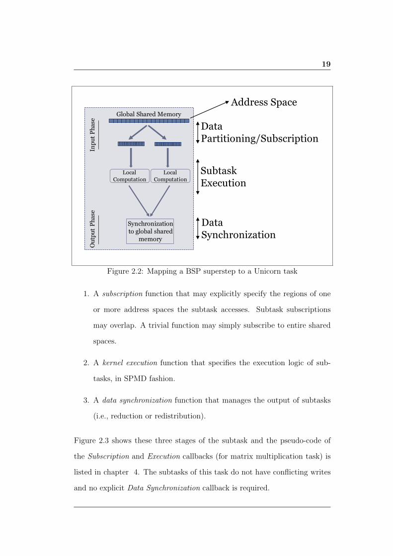
Figure 2.2: Mapping a BSP superstep to a Unicorn task
1. A subscription function that may explicitly specify the regions of one
or more address spaces the subtask accesses. Subtask subscriptions
may overlap. A trivial function may simply subscribe to entire shared
spaces.
2. A kernel execution function that specifies the execution logic of sub-
tasks, in SPMD fashion.
3. A data synchronization function that manages the output of subtasks
(i.e., reduction or redistribution).
Figure 2.3 shows these three stages of the subtask and the pseudo-code of
the Subscription and Execution callbacks (for matrix multiplication task) is
listed in chapter 4. The subtasks of this task do not have conflicting writes
and no explicit Data Synchronization callback is required.

20 Programming Model
Data Subscription
Kernel Execution
Data Synchro-nization (implicit,
reduce, redistribute)
Figure 2.3: Execution Stages of a Subtask
Note that explicitly specifying subtask subscriptions is not a requirement of
our model. However, due to a lack of virtual paging on GPUs one cannot au-
tomatically deduce this information at runtime without modifying subtask
code. Static code analysis is also not an attractive option as its scope is
limited and it restricts how kernels should be written. On CPUs, however,
automatic subscription inference is performed dynamically using POSIX’s
[32] mprotect feature to protect shared address spaces. On access by a sub-
task, that virtual page along with a few contiguous pages, is prefetched (if
necessary). With a pre-fetch of 5 pages (while multiplying two square matri-
ces with 4K elements each on an 8-node cluster with 12 CPU cores per node),
we measured this scheme to have a low overhead (10% - 15%) compared to
one with explicit subscriptions. A detailed analysis of this scheme, however,
is beyond the scope of this thesis.
A subtask may subscribe to multiple shared address spaces and multiple
discontiguous regions within each address space. This causes memory frag-
mentation and leads to poor cache performance. To alleviate this problem,
our model supports a notion of subscription views. A subtask kernel may

21
use the original global addresses (natural view) or a packed remapping of
addresses so the subscribed regions appear contiguous (compact view). The
compact view can save space and also yields better memory hierarchy usage
on GPUs, where memory is scarce (and virtual paging is not available). For
both views, a private copy of the subscribed regions of shared address space
is created for each potential writer, where it accumulates writes locally. On
completion of kernel execution conflicting spaces are combined. Read-only
regions are also fetched and cached locally on nodes but are shared among
all subscribing subtasks scheduled on that node. Note that using compact
views requires the subtask kernel to be modified to use re-mapped addresses.
1”’
1”
1’
1 2
3’
3 4
5”
5’
5 6
7’
7 8
Node 1 Node 2 Node 3 Node 4
Figure 2.4: Hierarchical Reduction - leaf nodes are subtasks, others are re-duced subtasks; dotted lines are inter-node data transfer
Although we support unified OpenCL subtask kernels for simplicity, better
performance may be achieved using specialized kernels for each architecture
type in the cluster (e.g. C++ for CPUs and CUDA for nVIDIA GPUs).
When writing specialized kernels, the programmer need not obsess about the
22 Programming Model
memory hierarchy of devices any more than one might with standard CPU
or CUDA implementations. This means that most existing kernel implemen-
tations can be effectively used as-is and can be debugged in sequential or
single GPU setup before being used.
We allow two primitives for synchronizing the output computed by differ-
ent subtasks: reduce and redistribute. The reduce operator allows an
application-provided callback function to combine output of two subtasks;
output that have been written to the same global address. Like standard
reduction, we assume it is commutative and associative. Our runtime sched-
ules reductions of the subtasks of a task in a hierarchical manner (Figure 2.4)
greedily as subtasks complete. The runtime first reduces memory of subtasks
executed on the same node. Once a node completes its local reductions, it is
reduced with another node that also has completed its local reductions. The
runtime executes inter-node reductions in a binary-tree fashion to improve
parallelism and reduce data transfer.
Reduction semantics require the local copies of the same address to be com-
bined to produce the final (or intermediate) copies. Sometimes the output of
the subtasks simply needs to be collated or reordered, e.g., to scatter-gather.
Performing this through reduction can be inefficient. We instead provide the
redistribute operator. Using this operator, the application can associate
a rank with different regions of its output address spaces. Our runtime then
ensures that all memory regions with the same rank are inserted consecu-
tively, in the order of subtask ID. Thus the regions are ordered in shared
address space by rank and within a rank by the writing subtask ID. This
operator can also be used to demand all-to-all broadcast or scatter-gather,

2.1 Data Subscriptions and Lazy Memory 23
more efficiently than through individual subscription.
2.1 Data Subscriptions and Lazy Memory
We acknowledge the programming overhead in explicitly specifying data sub-
scriptions before subtasks can access it. However, this is not a requirement of
our model. Rather, limitations of virtual paging prevent automatic inference
of data subscriptions. GPUs altogether lack virtual paging while CPUs are
limited to the granularity of a virtual memory page.
On CPUs, automatic subscription inference is performed using POSIX’s [32]
mprotect feature to protect shared address spaces. On access by a subtask,
that virtual page along with a few contiguous pages, is prefetched (if nec-
essary). With a pre-fetch of 5 pages, we measured this scheme to be only
10% slower than explicit subscriptions while multiplying two square matrices
with 4K elements each on an 8-node cluster with 12 CPU cores per node. We
call this delayed on-demand loading of subscription as lazy memory. Since
the mprotect feature can not protect a partial page, there could be conflicts
in case two subtasks write to different portions of the same page. However,
there are three ways to circumvent this limitation – the first involves padding
the address spaces such that every page is exclusively used by one subtask
only, the second employs page initialization by a sentinel value and a post-
processing step to take final value from the subtask that has changed the
sentinel and the third method is to resolve the conflict by implementing a
data reduction callback, which we do.
Due to a lack of virtual paging on GPUs, one cannot employ a similar tech-

24 Programming Model
nique to deduce subscription information at runtime. One possible alterna-
tive is force the programmer to access GPU’s global memory through some
wrapper that sets a flag (on GPU) for a polling CPU thread. The wrapper
makes the CPU thread fetch the required data and then DMA to GPU and
in the meantime the GPU kernel is made to sleep. However, this approach
is severely performance limiting. Another alternative is to infer subscription
using static code analysis of CUDA (or OpenCL or PTX assembly) code.
But we find its scope limited and it also restricts how kernels should be
written. Due to these operational limitations with GPUs and to maintain
programming uniformity, we focus this thesis on explicit data subscription by
application programs. Future improvements in GPU technology may provide
better solutions to this problem.

Chapter 3
Runtime System
This chapter describes the design of Unicorn’s runtime along with the moti-
vation for several design choices and trade-offs. The chapter also describes
several optimizations that enable our programming model. Unicorn’s run-
time system can be broadly decomposed into the following components. The
next few sections discuss these in more detail.
1. Device and Node Management
2. Shared Address Spaces
3. Network Subsystem
4. Pipelining
5. Scheduling
6. Software GPU Cache
7. Conflict Resolution
3.1 Device and Node Management
Unicorn consists of two major subsystems – network and scheduling. The two
comprise threads that manage cluster-wide operations like subtask scheduling

26 Runtime System
and data exchange between nodes. The scheduling subsystem is a two-level
hierarchy of threads with “scheduler thread” employing a “compute thread”
for every device (i.e., CPU core and GPU) on the node. The scheduler
thread issues commands to all compute threads and ensures that load among
those is balanced. The network subsystem is a collection of three threads.
All these threads serve similar purpose which is transfer of control messages
and data among nodes. However, different kinds of messages are handled
by different threads. One of these threads is designed for transfer of subtask
data (and accompanying data compression, if any) while the other two handle
the remaining messages (like task creation, address space ownership update,
etc.)
All threads in Unicorn serve a private priority queue that contains the com-
mands queued for it. These priority queues are revocable and commands in
queue can be removed before execution. Prioritization is required for task
ordering and issuing prefetch requests at lower importance than regular data
fetch. Revocation is required for features like work-stealing (section 3.5.3)
where subtask cancellation needs removal of queued commands.
Our commands are carefully designed to minimize the load on these queues.
For example, one of our commands allows execution of a set of subtasks
(specified as a range of subtask IDs) in one go. Our scheduler chooses the
device and the set of subtasks that should run on it. If the device is remote,
the scheduler requests the network subsystem to deliver the command to the
concerned queue.
For inter-node communications, the commands passed to the network subsys-
tem undergo a series of optimizations minimizing the number of MPI requests

3.1 Device and Node Management 27
and the volume of data transferred. These include buffering and grouping
disjoint requests into larger chunks when possible, filtering out duplicate re-
quests made by devices, and combining multiple outgoing messages to the
same node into one.
3.1.1 Runtime Internals
Controller
Profiling Manager
CommunicationManager
Device Manager
Task Manager
Scheduling Manager
Profiling andAnalysis Engine
Light Operations Threads
Heavy Operations Thread
CPU Compute Threads
GPU Compute Threads
Subtask Manager
Task Scheduler
Steal Agent
Work Stealing
Locality Aware
MemoryModule
pthreads
CUDA
OpenCL
MPI
Application
Network Subsystem Scheduling Subsystem Separate Thread
Figure 3.1: The design of the Unicorn runtime – Light orange region repre-sents the instance of the runtime on each node in the cluster
On initialization, Unicorn starts one MPI process per node in the cluster.
This process begins by creating an instance of controller. The controller
manages the creation, destruction and lifetime of all other runtime compo-
nents. These include Profiling Manager, Communication Manager, Device
Manager, Task Manager and Scheduling Manager. The last three modules
are part of the scheduling subsystem and the Communication Manager com-
prises the network subsystem. The controller is also the interface between the

28 Runtime System
application code and the Unicorn runtime. All application requests like cre-
ation and submission of tasks, creation and destruction of address spaces, etc.
pass through the controller. The runtime also executes user space callbacks
under the sandbox of the controller.
Once the controller initializes other runtime components, they directly talk
to each other without the controller’s involvement. All modules store diag-
nostic information with the Profiling Manager. The information collected by
the Profiling Manager on all nodes is accumulated on MPI master node at
application shutdown. This data may be dumped to stdout/stderr or may
be sent to Profiling and Analysis Engine for further processing. More infor-
mation on the kinds of analysis performed by the engine is present in chapter
6. The engine also converts the data into readily consumable graphical and
tabular formats. This information is mostly used for performance debugging
and diagnosis.
Task and subtask execution and all communication in Unicorn are carried
out asynchronously. For this reason, separate communication, scheduling
and device management components exist in the runtime. To support asyn-
chrony, these components accept commands with priority levels from other
components and execute them in dedicated threads. Being asynchronous is
also essential for optimizations like pre-fetching and for task pipelines that
overlap computation of subtasks with communication of others.
The Communication Manager carries out all inter-node communications over
MPI. All control messages (generated by the runtime) and all data trans-
fers (requested by executing subtasks) destined for remote nodes are routed
through the Communication Manager, which filters duplicate requests made

3.1 Device and Node Management 29
by various subtasks and also combines multiple requests targeted for same
destination node, whenever possible. Requests that involve subtask data
transfer are classified as heavy operations and are handled by a separate
thread. All other requests are light operations and are categorized into two
types – fixed size requests and variable size requests. Fixed size requests are
the ones whose data size is pre-known and special MPI optimizations that
re-use the same data buffers repeatedly are employed. Variable size data
requests have varying lengths and buffers are not pre-allocated for those.
Rather they are handled using MPI Probe in a separate thread. Segregating
heavy and light operations also allows critical control messages in the run-
time to be transferred quickly. This indirectly helps in keeping most runtime
threads active rather than waiting on a few commands.
The Device Manager handles all CPU cores and GPUs on a node. For each
device, it creates a dedicated compute thread, each of which is backed by an
exclusive priority queue. All commands that are targeted for execution on
a device are enqueued in the corresponding priority queue. Each compute
thread has a helper Memory Module. For the CPU compute threads, the
Memory Module manages sharing of read-only address space data and cre-
ation/destruction of virtual memory for local working copies of the address
space subscriptions of the subtasks. On the other hand, the Memory Mod-
ule for the GPU compute threads employ a software LRU cache for efficient
sharing of scarce GPU memory between subtasks. It also manages the cre-
ation and destruction of pinned memory buffers used for bidirectional DMA
transfers between CPU and GPU. CPU compute threads use pthreads un-
derneath while GPU ones use the CUDA runtime. Both may optionally use

30 Runtime System
OpenCL. We also explored using different processes (instead of threads) for
managing CPU and GPU devices. This helps sandboxing application code
but the performance implications of the approach render it impractical.
The Task Manager enqueues each task submitted by the application and
submits them for execution (to the Scheduling Manager) when all its depen-
dencies are fulfilled. This is accompanied by creation of a Subtask Manager,
Task Scheduler and Steal Agent. The Subtask Manager keeps track of the
subscriptions and data transfers of each subtask executing on the node. It
also tracks the subtask execution times, which helps estimate the relative
execution rates at different cluster devices. This also helps in determining
if a subtask is straggling and if it should be multi-assigned to some other
device. The Task Scheduler co-operates with the Subtask Manager and the
Scheduling Manager for executing a subtask and collecting its acknowledge-
ment. The Steal Agent’s role is limited to directing an incoming steal request
to the device with the highest load. The purpose of Steal Agent is to help
reduce the number of steal attempts in the cluster.
The Scheduling Manager handles scheduling of all tasks submitted by the
application. Like compute threads, the scheduling Manager has a dedicated
thread backed by an exclusive priority queue. The Task Scheduler of every
task enqueues subtasks in the Scheduling Manager’s queue and it schedules
them for local or remote devices (using the Communication Manager). When
a device finishes execution of its subtasks, an acknowledgement is sent to the
corresponding Task Scheduler through the Scheduling Managers on various
nodes communicating via their respective Communication Managers.
The default Unicorn scheduler is locality-oblivious and based upon two-level

3.1 Device and Node Management 31
work stealing assisted by Steal Agents. However, a task may opt for locality
aware scheduling, in which case data locality (on cluster nodes) is incorpo-
rated into scheduling decisions. Having a different system-wide Scheduling
Manager and a Task scheduler per task allows Unicorn to employ different
scheduling policies for different tasks running at the same time. However,
the common functionality is abstracted out into the system-wide Scheduling
Manager.
The next section lists the threads created by Unicorn’s runtime on every node
in the cluster. Subsequent sections of this chapter talk about the runtime in
greater detail and also explain the functionalities and design of the Network
subsystem and the Scheduling subsystem.
3.1.2 List of Threads
Unicorn runtime creates the following threads on each node in the cluster:
1. Fixed size network operations thread
2. Variable size network operations thread
3. Heavy network operations thread
4. Scheduler thread
5. One thread per CPU core or GPU device on the node
All our threads are light-weight and we do not dedicate any CPU core to
any of these. Rather, we let the management threads co-operate with device

32 Runtime System
threads running application code. The observed overhead of these man-
agement threads is small. For example, the image convolution experiment
(chapter 5) has a measured overhead of 0.2% of its total execution time.
3.2 Shared Address Spaces
Our runtime provides distributed shared address space to the application.
Unicorn tasks bind to one or more address spaces for input and output. This
is specified with access flags like read-only, write-only or read-write. Address
spaces can be used exclusively by tasks or they may be shared. Two examples
of address space sharing among tasks are – an output address space of a task
may serve as input to the next task, or an address space may contain constant
data serving as input to a series of tasks.
Address spaces can be thought of as an equal (and contiguous) allocation of
virtual memory on all intended nodes in the cluster. This allocation on all
nodes is equivalent and exists to provide a logical view of distributed memory.
The address spaces are distributed in the sense that generally their entire
data is not resident on any particular node in the cluster but distributed
over several nodes.
Subtasks (of tasks) operate upon the bound address spaces by means of sub-
scriptions. Read subscriptions define address space bytes required for com-
putations done by the subtask and write subscriptions define address space
bytes produced by the subtask (as output). These bytes can be a single
contiguous region of memory within the address space or these can be a set
of uniformly or randomly distributed contiguous memory regions within the

3.2 Shared Address Spaces 33
address space. For this reason, Unicorn allows a subtask to register multiple
subscriptions with the runtime (section 2). Note that each of these subscrip-
tions can be concisely specified using the quad tuple (offset, length, step,
size). This format enables applications to specify generally used contigu-
ous, block based and strided subscriptions in a few calls, which also directly
reduces the number of subscription calls the runtime processes per subtask.
As tasks execute on address spaces and their subtask subscriptions are pro-
cessed, address spaces are logically fragmented into memory regions defined
by these subscriptions. Internally, address spaces store these logical fragmen-
tations (called data regions) in the quad tuple format (offset, length, step,
size). Each of these data regions have an associated owner node in the cluster
and this owner node notionally contains the entire data corresponding to the
data region. The mapping of data regions to corresponding owner nodes is
stored in a directory called the address space ownership directory, or simply
the directory.
An application may create any number of address spaces from any node in
the cluster. The node on which an address space is incarnated is called its
creator node. Internally, Unicorn also assigns a master node to every address
space created by the application. As explained below, the master node serves
as an intermediary to enable efficient management of the directory. Master
nodes are chosen in round robin fashion to balance the load of all address
space routing requests among all cluster nodes. The master node contains the
master copy of directory for a given address space. Other nodes using that
address space generally contain a partial map: a subset of master ownership
directory. If these other nodes require a region that exists in their partial

34 Runtime System
map, they directly send region fetch requests to the corresponding owner.
On the other hand, if a region is not present in the partial map, they route
address space fetches through the master node. The master then consults its
ownership directory and forwards the request to the actual owner containing
the data region in question.
When an address space is created, it contains a single region. The ownership
directory on all nodes is updated to map that single region to the selected
master. As a subtask executes and commits its writes (originally in its private
view) to the address space, the node on which the subtask was executed
becomes the new owner of the data regions write-subscribed by the subtask.
(For multiple writers, the final owner is where the final reduction occurs). At
the end of a task, the new owner node records this ownership in its directory
and also sends this ownership update to the master. If the master observes a
new owner node, it updates its own map and forwards the ownership update
message to the previous owner(s), which also updates its map. All other
nodes always initialize their maps to point to the master at the end of the
task. Thus, at the beginning of a task all nodes map to themselves data
regions they own and point to master for all other data regions. The master,
however, always knows the true locations of all data regions in the address
space.
Unicorn tasks guarantee transactional semantics. This means that address
space ownership updates are reflected only at task boundaries and all sub-
tasks of a task see the same address space data during task execution. In
other words, even for an address space marked read-write, where a few sub-
tasks are updating the address space while a few are reading it, the ones that
3.2 Shared Address Spaces 35
are reading must not see the new data but read the state at the inception of
the task. Our address spaces achieve transactional semantics by deferring the
address space ownership updates till the end of the task. Since ownerships
are not modified during task execution, all subtasks continue to refer to the
original data location until task boundary. The following sequence of steps
define our delayed ownership update semantics –
1. All nodes hold information about write subscriptions of all locally com-
mitted subtasks in a local data structure. This information is a set ’S’
of quad tuples (offset, length, step, size).
2. At the end of the task, all nodes commit ’S’ into their address space
ownership directories and also send an ownership update message to
the master node. This message also carries the set ’S’.
3. The master node commits the received set ’S’ from every other node.
While commiting, it records the data regions that have changed owners
from last time and sends them another ownership update message.
4. All non-master nodes process the ownership update message from the
master and record master as the new owner of the data regions in the
message.
Note that we maintain a separate set ’S’ for every address space master node.
In other words, if a task employs three address spaces with two having the
same master node and the third having a different master node, we maintain
two such sets, one for each master. In case all address spaces used in a task
share the same master, only one set ’S’ is maintained and transferred.

36 Runtime System
Often, read subscriptions of subtasks (of a task) overlap. In such cases, it is
prudent that data once fetched (by a subtask) must not be re-fetched upon
request by another subtask. To accomplish this, our runtime records all data
fetched on a node in a separate address space directory. This directory is
temporary as its lifetime is bound to that of the ongoing task and is thus
called temporary ownership directory. At inception, the temporary directory
is a logical replica of the address space ownership directory on every node
and as data is fetched, it records the updates. For every read subscription
request from a subtask, the temporary directory is the one consulted and
not the main directory. This ensures that no data is transferred again during
the lifetime of the task. Note that this mechanism also conforms to the
transactional semantics guaranteed by our runtime. It further allows several
nodes to be simultaneously designated temporary owners of a data region
without the need of an explicit handshake (or ownership update message)
for data sharing.
At the end of the task, the data fetched for reading (and recorded in tempo-
rary directory) may become stale as data ownerships could have changed and
the new data owner could have written new data in that region. Thus, at
task boundaries, the temporary directories are simply discarded. However,
if a task does not write to an address space (and subscribes to it for reading
only), as an optimization its temporary directory entries are retained for the
subsequent task.
Figure 3.2 shows an address space and states of its address space ownership
directories and temporary ownership directories as it flows through two Uni-
corn tasks on a sample three node cluster. In the initial state, the address
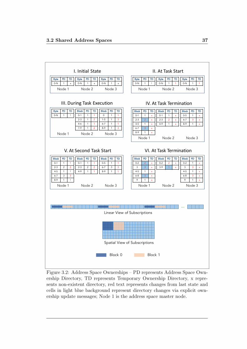
3.2 Shared Address Spaces 37
Byte PD TD
0-N 1 x
Byte PD TD
0-N 1 x
Byte PD TD
0-N 1 x
Node 1 Node 2 Node 3
I. Initial StateByte PD TD
0-N 1 1
Byte PD TD
0-N 1 1
Byte PD TD
0-N 1 1
Node 1 Node 2 Node 3
II. At Task Start
Byte PD TD
0-N 1 1
Block PD TD
0-1 1 1
2-3 1 2
4-6 1 1
7-9 1 2
Block PD TD
0 1 1
1-5 1 3
6-7 1 1
8-9 1 3
Node 1 Node 2 Node 3
III. During Task ExecutionBlock PD TD
0-1 1 x
2-3 2 x
4-5 1 x
6-7 3 x
8-9 1 x
Block PD TD
0-1 1 x
2-3 2 x
4-9 1 x
Block PD TD
0-5 1 x
6-7 3 x
8-9 1 x
Node 1 Node 2 Node 3
IV. At Task Termination
Block PD TD
0-1 1 1
2-3 2 2
4-5 1 1
6-7 3 3
8-9 1 1
Block PD TD
0-1 1 1
2-3 2 2
4-9 1 1
Block PD TD
0-5 1 1
6-7 3 3
8-9 1 1
Node 1 Node 2 Node 3
V. At Second Task StartBlock PD TD
0-2 2 x
3 3 x
4-5 1 x
6-8 3 x
9 1 x
Block PD TD
0-2 2 x
3-9 1 x
Block PD TD
0-2 1 x
3 3 x
4-5 1 x
6-8 3 x
9 1 x
Node 1 Node 2 Node 3
VI. At Task Termination
Block 0 Block 1
…Linear View of Subscriptions
Spatial View of Subscriptions
Figure 3.2: Address Space Ownerships – PD represents Address Space Own-ership Directory, TD represents Temporary Ownership Directory, x repre-sents non-existent directory, red text represents changes from last state andcells in light blue background represent directory changes via explicit own-ership update messages; Node 1 is the address space master node.

38 Runtime System
space master node (Node 1) owns the entire data. All directories point to
Node 1; temporary directories are null. In state II, a task starts and the
temporary directories on all nodes are logical replicas of the corresponding
main directories. In state III, Node 2 and Node 3 fetch data from Node 1
(for task execution) and the data brought in is recorded in their temporary
directories. The task terminates in state IV and subtasks that have executed
on each of the nodes commit their updates into the corresponding directories.
Noticing a change from previous state, Node 2 and Node 3 send ownership
update messages to Node 1 ands delete the temporary entries. In state V,
another task starts and a new temporary directory is instantiated on each
node. This task executes and upon termination commits writes to directories
in state VI. Again, Node 2 and Node 3 send ownership update messages to
Node 1. Upon receiving this message for block (or data region) 3, Node 1
notices a change from previous ownership (Node 2) and accordingly sends
another ownership update message to Node 2. Note that Unicorn consoli-
dates all ownership updates to be sent from a node to another and sends a
single unified message.
To theoretically analyze the overhead of our ownership update protocol, as-
sume a task executing on an N node cluster and using K address spaces K
> N. Our master selection mechanism ensures that every node is master of
at least one address space. Lets also assume that subtasks on node j make
Wij write subscriptions for address space i. This means the total number of
write subscriptions in the cluster is equal to
M =K∑i=1
N∑j=1
Wij
Updating the ownerships at the first instance would mean sending (or per-

3.2 Shared Address Spaces 39
haps broadcasting) at least M ownership update messages in the cluster.
However, by delaying these messages to task boundaries and by sending only
one ownership update message for all address spaces having the same master
node, we significantly reduce the number of ownership update messages gen-
erated in the cluster. In this example, every node being master of at least
one address space receives N-1 ownership update messages and every master
sends out a similar number of ownership update messages (in the worst case)
to non-masters. Thus, the maximum number of ownership update messages
possible with our protocol is 2N(N-1), which is significantly fewer than M.
Recall that Unicorn subtasks are also allowed to have overlapping write sub-
scriptions. In this case, subtasks are reduced by an application defined re-
duction operator. This reduction is a commutative and associative operation
and our runtime internally decides the node which becomes the final owner
of the overlapping data region post reduction. In this case, we do not send
any explicit ownership update at task boundary. Rather all nodes (except
master and the final owner) silently reset the new owner to the master node
whereas the master node and the final node record the final node as the new
owner.
Besides transactional semantics, our address spaces are designed for effi-
ciency. Our design ensures that no explicit ownership update messages are
required during task execution. Only at the end of the task, a few such
messages may be exchanged when the ownership of any data region changes.
To further limit the number of these messages, we aggressively reduce ad-
dress space fragmentation by combining adjacent directory records whenever
possible. Specifying subscriptions using block regions, further helps in mini-

40 Runtime System
mizing the number of directory entries. Unicorn’s runtime also ensures that
all ownership updates of an address space (at a task boundary) have finalized
before a subsequent task starts on any particular cluster node.
Our runtime implements address space ownership directory using an r-tree
[37] based map shared by all subtasks. Its key is the said quad tuple and the
value is the owner node. On a read query for a particular data region, the
corresponding quad tuple is looked up in the r-tree, which returns the set of
all overlapping quad tuples (along with their owner nodes). Each quad tuple
in this set is intersected with the data region in question and the data fetch
request of the intersecting regions is sent to the corresponding owner nodes.
If the owner node is the master node and it does not have the required data,
it re-routes the request to the node having the data, which now directly sends
data back to the requestor without involving the master node.
On the other hand, if an update needs to be recorded in the r-tree before
the new data region is inserted in it, all its overlapping quad tuples are first
deleted, the data region is subtracted from their union and the result and the
new region, both inserted. Before the insertion of any quad tuple, a query
is made on its four boundaries for the existing quad tuples. with the same
owner nodes as for the one being inserted. Any adjacent quad with the same
owner node (as the value to be inserted) is removed from the r-tree and a
unified quad is inserted.

3.3 Network Subsystem 41
3.3 Network Subsystem
Most distributed systems are bottlenecked by communication. Optimally
transferring data over the network is critical for sustained performance in a
cluster computing environment. Our network subsystem is optimized for per-
formance and works closely with compute threads and address spaces, merging
duplicate and overlapping requests, reducing both request and returned data
message counts and sizes. Besides, subtask data fetch requests are treated
at high priority while the prefetch requests for subtasks anticipated to run in
future are executed at a lower priority. Our network subsystem is also capa-
ble of compressing outgoing data and loss-lessly decompressing the same at
the recipient. This is especially important for large data transfers that are
otherwise too slow.
Recall that Unicorn runtime decomposes a task into multiple concurrent
subtasks. These subtasks may share part of their input data and thus may
subscribe to overlapping regions of input address spaces. Unicorn allows
subtasks to specify subscriptions as (offset, length) pairs or using quad tuples
(offset, length, step, count). The latter form is easy to use for strided or block
subscriptions. For each subtask subscription, our network subsystem queries
the address space directory for the corresponding data location in the cluster.
The query response may point to a local data location if the data is resident
locally on the node. In case the data is not locally resident, it may already be
enroute due to an earlier request or a new request must be initiated. In either
case the memory module returns a unique handle (internally implemented
like pthread signal-wait) on which the calling compute thread can wait till

42 Runtime System
the data arrives.
The network subsystem initiates a remote data fetch against this handle if the
request does not fully overlap with previous requests. The r-tree is again used
for overlap detection. When the remote data fetch completes, the handled is
notified and the waiting thread signaled. Note that the address space query
and handle creation happen atomically. This is done to ensure that any
other compute thread requiring the same data is returned the same handle
to wait on. In a typical scenario, a compute thread may wait on several such
handles and a handle may be waited on by several compute threads. In our
implementation, a subtask first issues all subscription requests and collects
all the remote handles it depends on and then an aggregate handle is created
which it actually waits on. The aggregate handle is unique to a compute
thread while the internal handles may be shared by several compute threads.
Handles created for remote data fetch for a subtask may be destined for one
or more nodes. Our network subsystem reduces latency of these network
requests by grouping all handles destined for the same remote node into one
underlying request on the network. The response, however, is separate for
different handles as this helps faster awakening of compute threads waiting
upon a subset of handles.
In addition to this, system latency is also reduced by piggy-backing several
control messages over other messages. For example, address space ownership
update messages (section 3.2) are often combined with subtask completion
acknowledgements. This prevents network congestion and makes way for
other high priority messages.
Unicorn tasks with conflicting writes (to output address spaces) are required

3.3 Network Subsystem 43
to define a data reduction callback (chapter 2). Subtask subscriptions in such
tasks are often large and may be entire address spaces altogether. Transfer-
ring such large address spaces (for reduction) over the network is generally
detrimental to system performance. In such cases, our network subsystem
compresses the address spaces before sending them across to other nodes.
Refer to section 3.7 for more details on this.
Our network subsystem internally employs three threads – one for fixed size
transfers, the second for variable size transfers and the third for heavy opera-
tions. The need for separate thread for fixed and variable sized data transfers
arises from MPI (our network subsystem’s backbone). While the former ones
are optimized by allocating the recipient buffer (of known size) in advance
and using persistent MPI commands repeatedly, the latter ones are received
using MPI Probe and post allocation of receiving buffer. We find that a
separate thread for MPI Probe works better. An example of variable size
data transfers in our runtime are ownership transfer messages which may
have a variable number of entries every time they are sent. These threads
are typically used to handle runtime’s control messages and many other task
execution messages. Hence we need to maintain a fast throughput on receiv-
ing and handling such messages. As a result, messages which are expected
to take longer are delegated from these threads to a separate heavy opera-
tions thread. These messages include subtask memory transfers, reduction
memory transfers (and associated compression/decompression), etc.

44 Runtime System
3.4 Pipelining
Overlapping computation with communication is critical to hiding heavy
data transfer latencies for subtasks. Data is transferred at two stages in our
runtime – the first is the transfer of data among nodes and the second is
the transfer of data from CPU to GPU. We intend to hide both these data
transfer costs by deploying subtask pipelines.
Our scheduler (section 3.5) assigns a set of subtasks to a device. These
subtasks are usually executed in the given order. Thus, while executing any
particular subtask, a device knows the next subtask it is likely to execute
(modulo steal). The device, thus, issues a communication request for the
next subtask when it starts executing any subtask. This behavior ensures
that while the devices are busy executing subtasks, the network does not
become idle and fetches data for future work.
Similarly, every GPU in the cluster is kept busy by employing a pipeline of
subtasks. The data is moved in and out of these GPUs along with the execu-
tion of one or more GPU kernels. Since data transfer to/from GPUs requires
DMA (and pinned memory), our runtime allocates and re-uses pinned buffers
for fast movement of data in and out of GPUs.
Besides pipelining, the bulk synchronous nature of our programming model
(that leads to the transactional design of our address spaces) plays a signifi-
cant role in hiding data transfer latency. The transactional design guarantees
that all subtasks (of a task) see the same input data (at any given location)
for the lifetime of the task. This enables us to use simple coherence protocol
where no address space ownership update messages are generated during task
3.5 Scheduling Subsystem 45
execution. Whatever data is pre-fetched to a node, remains valid through-
out the task, precluding the need for any further on-demand transfers for
any subtask that may need that data. This no-invalidation system helps in-
crease the percentage of time that network carries data messages (as opposed
to control messages for system correctness). The ability to have somewhat
coarse-grained tasks also helps reduce communication overhead.
3.5 Scheduling Subsystem
Unicorn’s scheduling subsystem is at the core of its performance. It is both
a proactive and reactive system. A number of optimizations are built into it
to ensure that appropriate scheduling decisions are taken in the first place.
However, device/network load as well as application characteristics are vari-
able. Our dynamic scheduler adapts to the situation efficiently. Results in
chapter 5 highlight the importance of such a dynamic scheme.
Our scheduler is work-stealing [44, 23] based and load is balanced among de-
vices by stealing unexecuted subtasks. We observe that the usual design gen-
erally suffices when devices with uniform computing capability are involved in
a computation. However, modern cluster environments have heterogeneities
in memory hierarchy and computing power of devices, network throughput
of nodes, device architecture (x86 64, Tesla, Fermi) and programming styles
(OpenCL/CUDA/C++), etc. Due to these variations, devices tend to differ
a lot in the effective throughput delivered for a particular computation. In
our experiments, we measured GPU performance higher than CPU perfor-
mance by more than an order of magnitude sometimes. In our tests, a BLAS

46 Runtime System
[24] based sequential implementation of multiplication of two dense square
matrices with 8K elements each (on Intel Xeon X5650) was outperformed
by a CUBLAS [17] based implementation (on Tesla M2070) by a factor of
33x+. Similarly, a BLAS based block LU-Decomposition on the GPU re-
ported 10x+ speedup over the sequential implementation. This disparity is
further aggravated in a cluster environment if the data is placed near faster
GPUs while the slower CPUs are on a remote node away from the data.
Scheduling subtasks across devices of widely different capabilities presents
its own challenges. Unicorn normally uses one cluster device as a computing
unit. However, to reduce disparity, a set of slow devices (usually CPU cores)
are made one computing unit (or work-group). Equivalently, a subtask is
now envisioned as a set of work-items and a single work-item is scheduled
per CPU core. The number of devices in a computing unit are dynamically
calibrated to yield the maximum performance. This work-group calibration
is performed locally on all nodes and all CPU cores on a node participate in
the formation of work-groups.
We also extend work stealing to account for subtask pipelining and underlying
device topology. To summarize, Unicorn employs a pipeline aware work
stealing scheduler accompanied by dynamic calibration of CPU work-groups.
The next few sub-sections describe these in detail, along with a scheduling
reconsideration technique, called multi-assign, for handling stragglers.
3.5.1 Work Stealing in Unicorn
The benefit of dynamic scheduling is that it responds not only to varying sub-
task load and compute unit capacity but also to varying network throughput.

3.5 Scheduling Subsystem 47
Unicorn scheduler begins by assigning an equal number of subtasks to each
device. Once a device nears completion, it steals subtasks from another
device. We employ two-level random stealing, where a compute unit first
attempts a local steal. On failure, it requests the steal-agent on a randomly
selected remote node, which in turn attempts to steal from its local units. Al-
though one might extend shared-memory algorithms to stealing over shared
address spaces or one sided MPI communication [23], we find the overheads
too high for that. On the other hand our runtime is already based on mul-
tiple asynchronous threads on each node and it is easier to use that runtime
infrastructure for load stealing without incurring loss in compute threads.
Recall that our pipelined schedule implies that the subtasks may be
1. idle,
2. waiting for data,
3. ready for execution, or
4. executing.
Our lock-free steal algorithm allows steal from any stage from idle to ready
for execution. (Steals from stage 4 is allowed as a special case and is discussed
later in section 3.5.3). The steal-agent on each node helps accomplish this
as it maintains the count of outstanding subtasks in each stage for all local
devices on its node and also monitors their execution rates. (Since we do not
model subtask heterogeneity, we simplify by using the past rate as a predictor
for future rate.) Thus, our two-level victim selection technique proceeds as
follows for device dij on node i:

48 Runtime System
1. In first attempt set victim v = i, otherwise, choose random victim v,
different from victims selected in this round. (Round resets when a
victim is found or no potential agents remain.)
2. Send steal request to (the steal agent of) node v. The steal request
includes the measured subtask execution rate, Rij of dij and its aggres-
sion level aij, a value in [1:3]. In our setup, we keep GPUs at maxi-
mum aggression level (i.e. 3) while the aggression of CPUs increases
with the number of consecutively failed steal attempts. Initially, CPUs
start with aggression 1 and reach the maximum level at N/2 consecu-
tive steal failures, where N is the number of nodes executing the task.
Note that all devices in the cluster record the number of steal requests
issued by them and their outcome (success or failure).
3. Agent v, selects device dvw that is expected to complete its queue the
last among all devices of node v. (i.e., the highest value of Qvw
Rvw, where
Q stands for the length of the queue at the given device). Agent v
considers subtasks in stage k only if aij >= k.
To further reduce the number of steal attempts in the cluster, a range of
subtasks is stolen. We compare the devices’ execution rates to decide the
quantum of the final steal: Qvw × Rij
Rij+Rvw. A task terminates when all its
device queues are empty.
In contrast, a one level stealing algorithm, where a device directly steals
from another randomly selected device, generates too many steal requests
and is not scalable. For example, if we assume N nodes and D devices per
node, and that at a time t, every device has a probability pt of having an

3.5 Scheduling Subsystem 49
empty queue. The probability of a one level random steal attempt being
successful is 1 – ptN×D
, while that of steal from a random steal agent is1 – pDt
N.
Our experiments described in chapter 5 also demonstrate this improvement.
We do not see the benefit of a deeper hierarchy (e.g. multiple steal-groups on
a node [40]) due to its management overheads. However, for larger clusters it
is possible that organizing nodes into hierarchical steal-groups will be useful.
3.5.1.1 ProSteal
As described earlier, Unicorn has all devices in the cluster aggressively over-
lap their current subtask computation with data transfer of the next potential
subtask. Various subtasks incur different data transfer latencies as the data
may already be locally available for some, while others may have to fetch
from one or more remote nodes. When a device turns idle and starts a steal
operation, it suspends its pipeline as it has no subtask whose data can be
fetched. After the stolen subtask arrives, the device restarts its pipeline
by initiating the stolen subtask’s data transfer. Had this subtask not been
stolen, its communication might have overlapped another subtask’s execu-
tion at the victim, which could have potentially completed the work faster.
In addition to this, GPU stealers suffer another pipeline hazard as they lose
the opportunity to overlap bi-directional data transfers between the device
and host CPU while they steal.
Figure 3.3 shows an example of a victim’s pipeline. The first three subtasks
execute normally – the computation of the first subtask gets overlapped
with the communication of the second and the computation of the second
gets overlapped with the communication of the third. However, subtask

50 Runtime System
Figure 3.3: Loss in victim’s pipeline due to work stealing
four and five get stolen and there is no subtask left in the compute thread’s
queue, whose communication could overlap with the computation of the third
subtask. This causes a stall and subsequent performance loss in the victim’s
pipeline. Note that the stealer has initiated the steal operation as its pipeline
has already stalled. Thus, a steal operation may cause a stall in both stealer’s
and victim’s pipelines.
Unicorn addresses this problem using a novel aggressive stealing approach,
called ProSteal where the stealer does not wait for its pipeline to exhaust.
Rather it steals with one or more subtasks still in the queue. Stealing early

3.5 Scheduling Subsystem 51
helps the stealer to overlap the stolen subtask’s communication with the
ongoing computations at its end. It is important to initiate the steal request
at the appropriate time as stealing too early may increase the number of
steal attempts and harm application performance. The optimal number of
outstanding subtasks when a device steals is computed as Rs × (Ls + Ld)
where Rs, Ls and Ld, respectively, are rate of subtask execution, steal latency
and data fetch latency of the stealer. In other words, the longer it takes
to prime the pipeline after flush, the more aggressive the stealer is. For
CPUs, which generally have a slow rate of subtask execution in comparison
to GPUs, the expression results in relatively less aggressiveness. Note that
this aggressiveness is different from the one described in section 3.5.1, where
the aggressiveness is actually a measure of desperation (and increases with the
number of consecutive steal failures) and affects the response of the requested
steal agent. On the other hand, ProSteal’s aggressiveness is a measure of
performance and determines how soon the stealer should initiate the steal
request.
A pipeline is perfect if it spends the same time in all its stages. Assuming
that our two stage pipeline (with communication being the first stage and
computation being the second stage) is perfect, we can obtain a theoretical
lower bound on the time lost in pipeline stall as Ls + Tp where Ls is the
steal latency and Tp is the time spent in any pipeline stage. However, in case
both stages are not uniform the time lost in pipeline stall will have an upper
bound of Ls + max(Ts1, Ts2) and a lower bound of Ls + min(Ts1, Ts2) where
Ts1 is the time spent in the first stage of the pipeline and Ts2 is the time spent
in the second stage of the pipeline. Using a value greater than max(Ts1, Ts2)

52 Runtime System
for Ld may lead to stealing too early and bringing in newer subtasks with a
few already in the stealer’s pipeline. This may cause throttle and ping pong
of subtasks (as the newly brought in subtasks, being pending, may be stolen
again). On the other hand, using a value smaller than min(Ts1, Ts2) for Ld
may be too small to prevent a pipeline stall. Thus, we use the average of
both Ts1 and Ts2 as the value of Ld. This yields good performance in our
experiments.
With ProSteal, we attempt to minimize the time lost in pipeline stall when
a GPU device empties its queue. It is difficult to predict Ls, Ts1 and Ts2
values for any particular subtask. Thus, for computing these numbers, every
Unicorn device uses the running average of the subtasks it has previously
executed. Secondly, we issue steal requests at subtask boundaries and not in
the middle of the pipeline. For this reason, we multiply our expression Ls+Ld
by the rate of subtask execution Rs. [3] presents a more comprehensive
analysis of this scheme. Results show that despite our approximations to the
theoretical bound, we avert GPU pipeline stalls by 80% (when using ProSteal
versus when not using it) on an average computed over the experiments
presented in section 5.3.1.2.
3.5.1.2 Locality-aware Scheduling
To reduce data fetch bottlenecks, Unicorn requires all subtasks of a task
be implemented with one dimensional or two dimensional spatial locality.
This means that consecutive subtasks access consecutive memory locations.
However, if a Unicorn task is implemented with little or no spatial locality
among subtasks, the application programmer can enable Unicorn’s locality-

3.5 Scheduling Subsystem 53
aware scheduling. When used, our locality-aware scheduler enriches schedul-
ing decisions by maximizing the re-use of locally resident data on nodes or
by minimizing the cost of fetching non-local data.
To maximize reuse of locally resident data on nodes, we compute an affinity
score of every subtask to every cluster node and possibly schedule subtasks
on nodes with high affinity towards them. To build such an affinity table
(subtasks versus nodes), we run an internal Unicorn task that computes this
information by analyzing address space directories on all cluster nodes. We
explore affinity score based on different parameters like maximize re-use of
locally resident data, minimize cost of transferring remote data, and minimize
estimated subtask execution time.
In Unicorn, a node’s address space directory is guaranteed to contain true
locations only for addresses in its local view. For all other addresses, it
points to address space’s master node (section 3.2), which points to the true
location. Hence, a node can only compute affinity of subtasks to itself but
not to other nodes. Thus, finding affinity of all subtasks to all nodes re-
quires a distributed computation in which each node finds its own affinity
to all subtasks. Another way to accomplish this is to compute this subtask-
node affinity table centrally. But a task may use multiple address spaces.
Centralized computation would require all master node’s directories to be
consolidated: leading to computation bottleneck in addition to large data
transfer.
For these reasons, our locality-aware scheduler works with only partial affinity
information on every node [4]. We let each node only compute every subtask’s
affinity to itself. This is a much smaller list with size equal to the number

54 Runtime System
of subtasks in one task. Only this list is centrally gathered and analyzed for
task scheduling: at one node for each task.
Unicorn’s default locality-oblivious scheduler initially computes the number
of subtasks to be assigned to devices on each node, under the premise that
all subtasks are likely to have equal load. We retain this as the first step
even for locality-aware scheduling. Starting from this number of subtasks to
be assigned to each node, we resort to a greedy approach (section 3.5.1.2.1)
to assign specific subtasks to specific nodes.
3.5.1.2.1 Greedy Scheduling
In our greedy scheduling approach, subtasks pick nodes round-robin. Each
time a subtask picks a node, the estimated completion time of that node is
incremented by a time-estimate based upon the subtask’s affinity score to
the node. Accordingly, a global task completion estimate is also updated.
Assume the computed affinity of subtask j to node v is Avj and T is a
user controlled function mapping Avj to time tvj. The estimate for node
v, Tv =∑
tvj ∀ subtasks j assigned to node v. The estimate of the task,
T = maxTv ∀ node v. Now, ∀ subtask j:
• assign j to node v such that the increase in T is the smallest.
• if two nodes v and w lead to the same increase (or no increase), assign
v if tvj < twj and w otherwise.
We discuss various mapping functions T in section 5.3.2. [4] theoretically
evaluates the greedy assignment algorithm and proves that greedily assigning

3.5 Scheduling Subsystem 55
every work-item to a node that will complete it with the lowest resulting
execution time is O(log n) competitive, with n being the number of nodes.
3.5.1.2.2 Locality-aware work stealing
The affinity information is also used during steal attempts where the victim
agent chooses the subtasks with the highest difference in affinity towards
the stealer. The victim computes a number – call it s – of subtasks to be
sent to the stealer on the basis of their relative rates of subtask execution
(i.e., the number of subtasks executed per second before the steal operation).
The victim, then, chooses the s subtasks with the highest difference between
their affinity to the stealer versus to the victim. As an aside, the stealer’s
affinity scores are not computed by the victim. We also do no include it with
every steal request. Rather, we piggyback nodes’ affinity scores on other data
transfer. Since stealing happens near the end of the task, a stealer’s affinity
array is highly likely to reach all potential victims with negligible overhead.
Nevertheless, if the affinity scores have not reached earlier, it comes with
the request. In section 5.3.2, we report performance improvements with this
scheme as compared to Unicorn’s locality oblivious work stealer, which may
allow a subtask with entire data on the victim’s node to be stolen by a
device on some other node with potentially no data, resulting in sub-optimal
performance.
3.5.2 Work-Group Calibration
An application may opt for work-groups to be created from multiple CPU
cores (on a node) in an attempt to assign them less work than intended in

56 Runtime System
a subtask. Otherwise, all the subtasks assigned to these cores may be stolen
by faster GPUs. In this case, a subtask is logically subdivided and multiple
work-items are created from it, with each work-item intended to run on one
CPU core of the work-group. The maximum size of work-group created for
a subtask is equal to the number of CPU cores on a node. The optimal size
of work-group (for subtasks of a task) is, however, computed using binary
search over the range [1, number of CPU cores].
Our algorithm requires at least two subtasks to bootstrap the binary search.
For the first subtask, the sizeof work-group is set to the number of CPU
cores on the node and for the second subtask the size of work-group is set
to half the number of CPU cores. Next, we compare the execution times of
both these subtasks. If the former one’s execution time is shorter, the size of
work-group for the third subtask is set to three-fourth the number of CPU
cores. On the other hand, if the latter execution time is longer, then the size
of work-group created for the third subtask is one-fourth the total number
of CPU cores. This dynamic adjustment continues until the end of the task.
This dynamic calibration ensures that changing system load is optimally
dealt with and CPU cores do not over-execute subtasks. Over-executing can
be detrimental not only to the subtasks executed by CPUs but to the ones
executed by GPUs as well. First, because several CPU cycles are required
to complete GPU’s work. In case, CPUs remain busy with other work, they
won’t be able to sufficiently keep the GPU pipeline busy by moving data
to/from pinned memory (and GPUs) and launching GPU kernels. Further,
large work on these slower cores also unnecessarily overload the memory and
network throughputs at these nodes.

3.5 Scheduling Subsystem 57
3.5.3 Multi-Assign
Work-stealing in Unicorn is non-preemptive. Hence, it is not possible to
migrate a running subtask from one node (or device) to another. If a subtask
takes a long time to finish, while other devices have become idle, Unicorn may
multi-assign that subtask, i.e., assign the same subtask to multiple devices.
At this stage, multiple instances of the same subtask may be running in the
cluster. However, the one that finishes first commits its results to the global
address space. All other running instances of the subtask are cancelled and
their output (in their private views) is discarded.
We employ a simple protocol to determine the subtask instances to be can-
celled. When a subtask is multi-assigned to a cluster device, it also memo-
rizes the device where the subtask’s original instance is running. The orig-
inal instance also records the device executing the multi-assigned instance.
Further multi-assignments are only allowed from the initial instance of the
subtask and a multi-assigned instance can not multi-assign further. Thus, at
any given time, the original instance knows where all the multi-assigned in-
stances are running and all the multi-assigned instances know the location of
the original instance. Whichever device finishes first, it informs the original
instance, which in turn sends cancellation messages to all others.
Multi-assign is implemented as a part of stealing. In particular, we allow a
subtask in ‘executing’ stage to also be stolen, while it is allowed to continue
executing. Such steals are only allowed when the steal request specifically
includes a multi-assign flag (i.e., when the stealing device is at maximum
aggression level (section 3.5.1)).

58 Runtime System
We multi-assign only if the stealing device’s estimated completion time (based
upon its observed execution rate) is less than the victim’s remaining esti-
mated completion time. We use the remaining time for victim because it has
already executed a part of the subtask at the time of multi-assign. Thus,
the time it has already spent in execution of the subtask is subtracted from
its total estimated time. As an additional heuristic, a subtask is only multi-
assigned to a device on a different node or to a different device type on the
same node (CPU subtasks are multi-assigned to GPU and vice versa). This
reduces the chance of slow execution on the re-assigned device as well. Exper-
iments show significantly faster completion times due to multi-assignment.
This is especially useful in networked environments, where the effective data
transfer bandwidths may be variable and a device on a node with slow link
may not receive its input fast enough, delaying the entire task.
3.5.3.1 Subtask Cancellation
Post multi-assign, only the earliest completing instance of subtask is allowed
to commit its output. All others are sent cancellation messages. In our im-
plementation, subtask cancellations are done gracefully if they happen to be
executing Unicorn’s code at the time of cancellation. However, cancellation
is complicated in case subtasks are executing application code at the time of
cancellation.
We cancel a CPU subtask by performing a longjmp out of the application
code. However, this has the potential to leak resources or leave them in
an inconsistent state. For this reason, we require application kernels to be
self-confined and not access global state that requires explicit cleanup. Ap-

3.5 Scheduling Subsystem 59
plications that cannot conform to this requirement may opt to disable the
multi-assign feature.
Further, the current state of technology on GPUs does not allow clean can-
cellation of an executing kernel. The entire GPU context may be destroyed
but that has a high overhead and may also leave the GPU in an inconsistent
state temporarily. For this reason, we currently do not multi-assign GPU
subtasks in case they have copied data from CPU to GPU (and started ker-
nel execution). However, if GPU technology matures and provides a low
overhead kernel termination in future, we can enable GPU multi-assignment
freely.
3.5.4 Scheduling Across Task Barriers
The Unicorn programming model introduces a task barrier at the end of ev-
ery task. This existence of the barrier simplifies application programs and
helps programmers logically think through the parallel program’s control
flow. However, barriers do incur overhead on the overall application per-
formance, even with good load balance. To circumvent this overhead, we
maintain only a logical barrier but dilute its physical presence by allowing
subtasks (of a subsequent task) to be scheduled before the barrier imposed
by the earlier task, as soon as their dependencies are satisfied. To support
this, we pre-process subtask subscriptions of all submitted tasks and build a
subtask data dependency graph. Any subtask which has all its dependencies
satisfied can be allowed to start without waiting for the barrier. A detailed
analysis of this aggressive scheduling scheme and the types of applications
where they accrue benefit, however, is beyond the scope of this thesis.

60 Runtime System
3.5.5 Scheduling Concurrent Tasks
The current implementation of Unicorn allows multiple simultaneous tasks
only if their subscribed address spaces are disjoint or if they are read-only.
When a task is ready for execution, all its subtasks are added to execution
queues of various compute devices. Thereafter, they are scheduled, stolen
and multi-assigned as usual. An application can also specify a priority with
a task to control its scheduling.
3.6 Software GPU Cache
Moving data between CPUs and GPUs is a relatively expensive operation.
For optimal performance, it is important to reduce the frequency and volume
of such data copies. Subtasks of a Unicorn task are allowed to have overlap-
ping subscriptions. In such situation, it is beneficial to transfer data from
CPU to GPU only once and use it for as many subtasks as possible. Simi-
larly, output produced by a Unicorn task may serve as input to a subsequent
task. In this case, data can be retained on GPUs at the end of the task in
anticipation that a subtask (of a future task) may be scheduled on the same
GPU.
Our runtime maintains an on-GPU software cache to optimize DMA transfers
to the device. The cache allows a GPU to skip a data transfer in case the data
is already resident. This scheme is suitable for both the scenarios described
above, i.e., multiple subtasks of a task share read-only data and data written
by a subtask of a task is later read by a subtask of another task. An exclusive

3.7 Conflict Resolution 61
instance of GPU cache is created for every GPU in the cluster.
Unicorn’s runtime supports four GPU cache eviction policies – LRU (least
recently used), MRU (most recently used), LFU (least frequently used) and
MFU (most frequently used). The eviction policies come into play when
GPU is low on global memory space and memory needs to be freed up by
evicting one or more cache entries. LRU scheme evicts the least recently used
subscription, MRU evicts the most recently used subscription, LFU evicts the
least frequently used subscription while MFU evicts the most frequently used
subscription. By default, our current implementation employs LRU cache
eviction policy. Depending upon the nature of the application, other cache
eviction policies may be requested. A study of performance implications of
these policies is presented in section 5.6.3.
Unlike hardware caches, we do not have a concept of cache lines that get
invalidated. Rather, we invalidate entire subtask subscription. A study on a
true cache implementation versus ours may provide interesting pointers for
a better cache design. But this is beyond the scope of this thesis.
3.7 Conflict Resolution
Unicorn subtasks may subscribe to overlapping regions in an address space.
The runtime treats this as a write conflict among subtasks and the application
must explicitly specify a reduction mechanism to resolve the conflict. The
output, otherwise, is not defined. Unicorn runtime provides a range of inbuilt
reduction operators which an application may use. Applications are also free
to define custom reductions.

62 Runtime System
Unicorn treats reduction as a first-class citizen and the output of subtasks
are aggressively reduced as soon as they are ready. Thus, at any given time,
a few subtasks may be in the execution stage while a few others may be in
reduction stage. Aggressively performing reductions help in reducing overall
execution time as these are executed during the time subtasks await their
remote subscriptions to be fetched. Secondly, this reduces memory pressure
on the system. As soon as two subtasks reduce, the memory of one of these
is freed. Steal attempts are made only if there is no reduction to perform.
Note that subtasks may subscribe to an entire address space. This is the
worst case for reduction as all subtasks conflict with each other. To efficiently
perform reduction, Unicorn employs the following three optimizations:
1. Despite subscribing to entire address spaces, subtasks may only write
to a few disjoint portions of the address space. We uses POSIX’s mpro-
tect feature to determine the VM pages touched a subtask and invoke
conflict resolution on those pages only.
2. GPU kernels are by design multi-threaded. On CPUs, we use OpenMP’s
parallel for construct to speedup execution of inbuilt reduction opera-
tors.
3. Before transmitting data to remote nodes for reduction, it is compressed
by our network subsystem (section 3.3). To optimize reduction, we
also compress data before transmitting from GPUs to CPUs. Unicorn
provides a few in-built compression algorithms but applications may
also provide their own.
Chapter 5 describes the PageRank experiment implemented over Unicorn,

3.7 Conflict Resolution 63
where entire address spaces are subscribed. The results of the experiment
show that Unicorn achieves good scalability and reduction is performed quite
efficiently.

64 Runtime System

Chapter 4
Pseudo Code Samples
Unicorn programs are written as a graph of tasks communicating through
address spaces. A task reads from its input address spaces and writes to
its output ones that may serve as input to one or more subsequent tasks.
During execution, subtasks of a task are required to subscribe to address
space regions they want to operate upon. Once the subscriptions are speci-
fied, Unicorn runtime optimally transfers the subscribed data to the device
where subtask is executing and creates private views for subtask’s writes to
be accumulated.
Subtasks communicate with our framework through a series of callback func-
tions - the data subscription callback defines the regions of the global shared
memory a subtask would read-from or write-to (collectively called subtask
subscription), the kernel execution callback is the actual computation logic
of the subtask written either in hardware’s native language like C/C++ for
CPUs and CUDA for GPUs, or in a high level language like OpenCL [55]
which caters to both CPUs and GPUs, and the data synchronization callback
which defines how conflicting writes from different subtasks be merged before
committing to the global shared address space.
This section presents pseudo code skeletons of two application programs: one
computes Matrix Multiplication and the other computes two dimensional
Fast Fourier Transform (2D-FFT) using our runtime. The former example

66 Pseudo Code Samples
is implemented using one Unicorn task whereas the latter one employs two
Unicorn tasks - the first one computes 1D-FFT on matrix rows while the
second one computes 1D-FFT on matrix columns.
Listing 4.1 shows the pseudo code skeleton of a Unicorn program that multi-
plies two square matrices to produce the result matrix. The matrix multiply
function takes matrix dimension and block dimension as input. The former
is the number of elements in rows/columns of the square matrices while
the latter is the number of elements in rows/columns of each subtask. For
simplicity, the code sample assumes that matrix dimension is divisible by
block dimension. Line 5 of the code registers the data subscription callback
and line 6 registers an OpenCL based subtask execution callback. This call-
back is executed on both CPU and GPU devices in the cluster. Lines 11 to
13 of the program create three address spaces - one for each matrix involved
in the computation. The output (or result) matrix is logically divided into
blocks of size block dimension ∗ block dimension. The program creates a
task and a subtask for each of these logical blocks of the output matrix (line
20). The line also creates an instance of the task configuration struct mat-
mul conf. Task configuration is generally used for small task-wide read-only
that all subtasks should see. Unicorn ensures that the configuration is auto-
matically transported to all CPU and GPU devices in the cluster. Thereafter,
lines 21 to 23 specify access modifiers for each of the three address spaces.
Both input address spaces are accessed in read-only fashion while the output
address space is write-only. Finally, line 24 submits the matrix multiplication
task to the Unicorn runtime for asynchronous execution. The program waits
for the asynchronous task to finish on line 25.

67
1 struct matmul conf { s i z e t matrix dimension ,b lock d imens ion ; } ;
2 matrix multiply ( matr ix dimension , b lock d imens ion )3 {4 key = ”MATMUL” ;
5 register callback ( key ,SUBSCRIPTION,matmul subscr ipt ion ) ;
6 register callback ( key , OPENCL, ” matmul ocl ” ,” prog . o c l ” ) ;
7 i f ( get host ( ) == 0) // Submit task from s i n g l e host8 {9 // c r e a t e address spaces
10 s i z e = matr ix dimens ion ∗ matr ix dimens ion ∗s izeof ( f loat ) ;
11 input1 = malloc shared ( s i z e ) ;12 input2 = malloc shared ( s i z e ) ;13 output = malloc shared ( s i z e ) ;
14 i n i t i a l i z e i n p u t ( input1 ) ; // a p p l i c a t i o n code15 i n i t i a l i z e i n p u t ( input2 ) ; // a p p l i c a t i o n code
16 // f i n d b locks per dimension ( assumes d i v i s i b i l i t y )17 block count = matr ix dimens ion / b lock d imens ion ;
18 // c r e a t e task with one subtask f o r every block o fthe output matrix
19 subtasks = block count ∗ block count ;20 task = create task ( key , subtasks ,
matmul conf ( matrix dimension , b lock d imens ion ) ) ;
21 bind address space ( task , input1 , READ ONLY) ;22 bind address space ( task , input2 , READ ONLY) ;23 bind address space ( task , output , WRITE ONLY) ;
24 submit task ( task ) ;25 wait for task completion ( task ) ;26 }

68 Pseudo Code Samples
27 }
Listing 4.1: Unicorn program for square matrix multiplication
Unicorn callbacks for the matrix multiplication application are shown in list-
ing 4.2. Each subtask computes its part in the result matrix. For that, it
subscribes to corresponding rows of the first input matrix and corresponding
columns of the second input matrix (lines 23-25) in the data subscription call-
back. The OpenCL kernel launch configuration is specified on line 27 and the
OpenCL callback is implemented from line 30 onwards. This callback reads
from the subtask’s subscriptions in both input matrices and computes the
subtask’s output. For higher performance, Unicorn also allows the OpenCL
subtask kernel to be substituted by two native kernels - one for CPU (in
C/C++) and the other for GPU (in CUDA).
1 matmul subscription ( task , device , subtask )2 {3 matmul conf∗ conf = ( matmul conf ∗) ( task . conf ) ;4 block count = conf→matr ix dimens ion /
conf→ block d imens ion ;
5 block row = ( subtask . id / b lock count ) ;6 block column = ( subtask . id % block count ) ;
7 matr i x row s i z e = conf→matr ix dimens ion ∗s izeof ( f loat ) ;
8 b l o c k r o w s i z e = conf→ block d imens ion ∗s izeof ( f loat ) ;
9 b l o c k r o w o f f s e t = block row ∗conf→ block d imens ion ∗ matr i x row s i z e ;
10 b l o c k c o l u m n o f f s e t = block column ∗conf→ block d imens ion ∗ s izeof ( f loat ) ;
11 b l o c k o f f s e t = b l o c k r o w o f f s e t +b l o c k c o l u m n o f f s e t ;

69
12 /∗13 ∗ Spec i f y s u b s c r i p t i o n s14 ∗ A block s u b s c r i p t i o n i s de f ined by o f f s e t , s i z e ,
s tep and count15 ∗ F i r s t input matrix s u b s c r i b e s to a l l b locks in
the row block row16 ∗ Second input matrix s u b s c r i b e s to a l l b locks in
the column block column17 ∗ Output matrix s u b s c r i b e s to the block at row
block row and column block column18 ∗/
19 block subscription info bs in f o0 ( b l o c k r o w o f f s e t ,mat r ix row s i z e , mat r ix row s i z e ,conf→ block d imens ion ) ;
20 block subscription infobs in f o1 ( b l o ck co lumn o f f s e t , b l o ck row s i z e ,mat r ix row s i z e , conf→matr ix dimens ion ) ;
21 block subscription info bs in f o2 ( b l o c k o f f s e t ,b l o ck row s i z e , mat r ix row s i z e ,conf→ block d imens ion ) ;
22 // Bind s u b s c r i p t i o n s to address spaces by index23 subscribe ( task . id , dev i ce . id , subtask . id , 0 ,
b s i n f o0 ) ;24 subscribe ( task . id , dev i ce . id , subtask . id , 1 ,
b s i n f o1 ) ;25 subscribe ( task . id , dev i ce . id , subtask . id , 2 ,
b s i n f o2 ) ;
26 // OpenCL ke rne l launch c o n f i g u r a t i o n27 set launch conf ( task . id , dev i ce . id , subtask . id ,
. . . ) ;28 }
29 // OpenCL Kernel ( should go in to prog . o c l f i l e )30 matmul ocl ( task , device , subtask )31 {32 matmul conf∗ conf = ( matmul conf ∗) ( task . conf ) ;

70 Pseudo Code Samples
33 f loat ∗ input1 = ( f loat ∗) subtask . s u b s c r i p t i o n [ 0 ] ;34 f loat ∗ input2 = ( f loat ∗) subtask . s u b s c r i p t i o n [ 1 ] ;35 f loat ∗ output = ( f loat ∗) subtask . s u b s c r i p t i o n [ 2 ] ;
36 . . . OpenCL Matrix M u l t i p l i c a t i o n Code . . .37 }
Listing 4.2: Unicorn callbacks for square matrix multiplication
Listing 4.3 shows the pseudo code for 2D-FFT. The experiment firstly per-
forms a 1D-FFT along the input matrix rows (lines 22-29) and then performs
1D-FFT along the columns of the input matrix (lines 30-39). Different call-
backs are registered for both kinds of FFTs. Subscriptions for the row FFT
task are specified on lines 9-10 while the ones for the column FFT task are
registered on lines 11-12. Line 35-37 ensure that the column FFT uses the
output address space of the row FFT as its input. The input address space
of the row FFT contains the final output after execution of the column FFT
task.
1 struct complex { f loat r ea l , imag ; } ;2 struct f f t c o n f { s i z e t rows , c o l s ; } ;
3 ROWS PER SUBTASK = 128 ;
4 // Assumes matr ix rows and m a t r i x c o l s are d i v i s i b l eby ROWS PER SUBTASK
5 f ft 2d ( matrix rows , m a t r i x c o l s )6 {7 r o w f f t k e y = ”FFT ROW” ;8 c o l f f t k e y = ”FFT COL” ;
9 register callback ( r ow f f t k ey , SUBSCRIPTION,f f t r o w s u b s c r i p t i o n ) ;
10 register callback ( r ow f f t k ey , OPENCL,” f f t r o w o c l ” , ” prog row . o c l ” ) ;

71
11 register callback ( c o l f f t k e y , SUBSCRIPTION,f f t c o l s u b s c r i p t i o n ) ;
12 register callback ( c o l f f t k e y , OPENCL,” f f t c o l o c l ” , ” p r o g c o l . o c l ” ) ;
13 i f ( get host ( ) == 0) // Submit task from s i n g l e host14 {15 // c r e a t e address spaces16 s i z e = matr ix rows ∗ m a t r i x c o l s ∗ s izeof ( complex ) ;17 input = malloc shared ( s i z e ) ;18 output = malloc shared ( s i z e ) ;
19 i n i t i a l i z e i n p u t ( input ) ; // a p p l i c a t i o n data
20 // c r e a t e task c o n f i g u r a t i o n21 f f t c o n f f f t t a s k c o n f ( matrix rows , m a t r i x c o l s ) ;
22 /∗ Row FFT Task ∗/
23 // c r e a t e task with one subtask per row24 nsubtasks = matr ix rows / ROWS PER SUBTASK;25 task = create task ( r ow f f t k ey , nsubtasks ,
f f t t a s k c o n f ) ;
26 bind address space ( task , input , READ ONLY) ;27 bind address space ( task , output , WRITE ONLY) ;
28 submit task ( task ) ;29 wait for task completion ( task ) ;
30 /∗ Column FFT Task ∗/
31 // c r e a t e task with one subtask per column32 nsubtasks = m a t r i x c o l s / ROWS PER SUBTASK;33 task = create task ( c o l f f t k e y , nsubtasks ,
f f t t a s k c o n f ) ;
34 // Swap both the address spaces35 swap( input , output ) ;
36 bind address space ( task , input , READ ONLY) ;

72 Pseudo Code Samples
37 bind address space ( task , output , WRITE ONLY) ;
38 submit task ( task ) ;39 wait for task completion ( task ) ;40 }41 }
Listing 4.3: Unicorn program for 2D-FFT
Listing 4.4 describes callbacks of both 1D-FFTs. Each subtask of the row
FFT task computes 1D-FFT on a contiguous set of 128 rows while each
subtask of the column FFT task computes 1D-FFT on a contiguous set of
128 columns of the input matrix. The subscription for row FFT task is a
contiguous chunk of 128 rows (lines 4-9) while the subscription for column
FFT task is a scattered set of rows of 128 elements (lines 24-31).
1 fft row subscription ( task , device , subtask )2 {3 f f t c o n f ∗ conf = ( f f t c o n f ∗) ( task . conf ) ;4 r o w s s i z e = ROWS PER SUBTASK ∗ conf→ c o l s ∗
s izeof ( complex ) ;
5 // sub s c r i b e us ing o f f s e t and length6 subscription info s i n f o ( subtask . id ∗ row s i ze ,
r o w s s i z e ) ;
7 // sub s c r i b e to input and output memory by index8 subscribe ( task . id , dev i ce . id , subtask . id , 0 , s i n f o ) ;9 subscribe ( task . id , dev i ce . id , subtask . id , 1 , s i n f o ) ;
10 // OpenCL ke rne l launch c o n f i g u r a t i o n11 set launch conf ( task . id , dev i ce . id , subtask . id ,
. . . ) ;12 }
13 // OpenCL Kernel ( should go in to prog row . o c l f i l e )14 f ft row ocl ( task , device , subtask )15 {

73
16 f f t c o n f ∗ conf = ( f f t c o n f ∗) ( task . conf ) ;17 complex∗ input = ( complex ∗) subtask . s u b s c r i p t i o n [ 0 ] ;18 complex∗ output = ( complex ∗) subtask . s u b s c r i p t i o n [ 1 ] ;
19 . . . OpenCL 1D FFT Code . . .20 }
21 f ft col subscription ( task , device , subtask )22 {23 f f t c o n f ∗ conf = ( f f t c o n f ∗) ( task . conf ) ;24 o f f s e t = ROWS PER SUBTASK ∗ subtask . id ∗
s izeof ( complex ) ;25 c o l s s i z e = ROWS PER SUBTASK ∗ s izeof ( complex ) ;26 s t e p s i z e = conf→ c o l s ∗ s izeof ( complex ) ;
27 // sub s c r i b e us ing o f f s e t and length28 block subscription info b s i n f o ( o f f s e t , c o l s s i z e ,
s t e p s i z e , conf→ rows ) ;
29 // sub s c r i b e to input and output memory by index30 subscribe ( task . id , dev i ce . id , subtask . id , 0 ,
b s i n f o ) ;31 subscribe ( task . id , dev i ce . id , subtask . id , 1 ,
b s i n f o ) ;
32 // OpenCL ke rne l launch c o n f i g u r a t i o n33 set launch conf ( task . id , dev i ce . id , subtask . id ,
. . . ) ;34 }
35 // OpenCL Kernel ( should go in to p r o g c o l . o c l f i l e )36 f f t co l o c l ( task , device , subtask )37 {38 f f t c o n f ∗ conf = ( f f t c o n f ∗) ( task . conf ) ;39 complex∗ input = ( complex ∗) subtask . s u b s c r i p t i o n [ 0 ] ;40 complex∗ output = ( complex ∗) subtask . s u b s c r i p t i o n [ 1 ] ;
41 . . . OpenCL 1D FFT Code . . .42 // Succ e s s i v e e lements are conf→ c o l s apart43 }
Listing 4.4: Unicorn callbacks for 2D-FFT

74 Pseudo Code Samples

Chapter 5
Experimental Evaluation
We have implemented several coarse-grained scientific computation bench-
marks over Unicorn. These include image convolution, matrix multiplication,
LU matrix decomposition, two-dimensional fast Fourier transform (2D-FFT)
and Page Rank. These benchmarks have well known parallelizations and are
diverse enough for studying different kinds of complexities. Image convolu-
tion, although embarrassingly parallel, has a unique requirement of fringe
around the image. Matrix multiplication is computationally intensive with
heavy data transfer requirements. LU decomposition has a nested task hier-
archy, 2D-FFT involves a parallelization-unfriendly matrix transpose opera-
tion and finally Page Rank is a map-reduce based computation. The goal of
these experiments is to assess conditions under which our runtime responds
well.
Our experimental cluster consists of fourteen nodes, each equipped with two
6-core Intel Xeon X5650 2.67 GHz processors and two Tesla M2070 GPUs.
The nodes run CentOS 6.2 with CUDA 5.5. For communication, we use Open
MPI [31] 1.4.5 (over SSH) over an InfiniBand [1] network with 32Gbps peak
bandwidth. Unless stated otherwise, the input address spaces are randomly
distributed (as 2048 × 2048 blocks) over the cluster nodes and our runtime
transparently moves data on-demand to other nodes, as the program exe-
cutes.

76 Experimental Evaluation
Our runtime allows restricting applications to only certain cores, e.g., only
CPU cores, only GPUs, or both, However, CPU cores, being main OS vehi-
cles, are not used purely for computation but also other support functions like
CPU-GPU data transfers, GPU kernel launches, network data transfers, etc.
When subtask data usage is high (e.g., in several hundred MBs per subtask),
significant CPU load is observed in CPU↔GPU data transfers. Based on our
empirical analysis, we withhold upto two CPU cores (per node) from subtask
execution when both CPUs and GPUs are requested by an application. In
section 5.7.1, we study the performance impact of varying the number of
CPU cores employed in computations. This also provides an insight into the
library’s runtime overheads.
Many of our experiments use subtasks of size 2048× 2048. This empirically
determined size works well for both CPUs and GPUs. The size is not too
large for CPUs (to cause frequent cache misses) and not too small for GPUs
(to cause their under-utilization). In section 5.5.3, we present the impact of
varying subtask size on performance.
We first discuss the implementation of the selected benchmarks over Unicorn
and then present how these scale with an increasing number of nodes. We
also compare the performance of these implementations to the reference cases
when only CPU cores and when only GPUs are used in the cluster.
Next, we evaluate Unicorn’s work-stealing based scheduling by comparing it
with a work-sharing scheduling scheme. We also compare the overheads of
one-level work-stealing with a naive two-level technique and ProSteal (sec-
tion 3.5.1.1) – a scheduling optimization which proactively steals subtasks
before the devices finish their assigned subtasks. Next, we evaluate Uni-
77
corn’s locality-aware scheduling, which is used in cases when the subtasks of
our experiments are written without any particular order of spatial locality.
As described in section 3.5.1.2, the affinity of subtasks to nodes is evaluated
in a separate internally created Unicorn task. The outcome of this task is
a table that gives a score to a subtask-node pair. The score can be based
on several criterion. In our evaluation, we evaluate four different heuristics
for computing the affinity (or locality) score. The first three heuristics re-
spectively maximize reuse of local data on a node (i.e., score awarded to a
subtask-node pair is directly proportional to the amount of subtask’s input
data resident on the node), minimize the number of remote data transfer
events per subtask, and minimize the estimated data transfer time per sub-
task. The fourth one is a hybrid heuristic called Derived Affinity, which
computes scores by minimizing both remote transfer events and estimated
data transfer time per subtask.
The scheduling results are followed by a study of load balance achieved by
our runtime. Here, we study the finishing times of various cluster devices
involved in computations. The closer the devices finish to each other, the
better the load is balanced. We also experiment with changing the input
data location in the cluster and observe that the load still remains balanced
as our runtime automatically moves more computations to the node with
more resident data.
Next, we test our runtime’s resilience to data organization and subtask sizes
used in computations. We first change the initial placement (in the cluster) of
input data for various experiments and study the response of our runtime to
various commonly used patterns. Next, we change subtask sizes for various

78 Experimental Evaluation
experiments and study its performance implications.
Next, we study various optimizations presented in section 3. These include
multi-assign, pipelining and gpu caches. This is followed by a study of Uni-
corn’s overheads where we focus on time spent in runtime versus application
code. We also vary the number of CPU cores employed in computations
requiring both CPUs and GPUs in the cluster and study the response of the
experiments.
All measurements are based on at least three trials. Results are presented
for the sample that reported minimum execution time.
5.1 Unicorn Parallelization of Benchmarks
In our image convolution experiment all color channels of a 24-bit RGB
image of size 65536 × 65536 are convolved with a 31 × 31 filter. The input
image is stored in a read-only address space (initially distributed randomly
across the cluster nodes), logically divided into 1024 blocks of size 2048 ×
2048. Each block is convolved using a separate subtask. However, because
convolution at boundaries requires data from adjoining blocks, the input
memory subscription of a subtask overlaps with other subtasks’, usually at
all four boundaries. The output image is generated in a write-only address
space.
In the matrix multiplication experiment two dense square matrices of size
216×216 each are multiplied to produce the result matrix. Each input matrix
is stored in a read-only address space and the result matrix is stored in a
write-only address space of the task. The output matrix is logically divided

5.1 Unicorn Parallelization of Benchmarks 79
into 2048 × 2048 blocks and computation of each block is assigned to a
different subtask (which subscribes to all blocks in the corresponding row of
the first input matrix and all blocks in the corresponding column of the second
input matrix). The CPU subtask callback is implemented using a single-
precision BLAS [24] function and the GPU callback uses the corresponding
CUBLAS [17] function.
For the in-place block LU Decomposition [21] experiment, the input matrix
(216 × 216) is kept in a read-write address space and is logically divided
again into 2048× 2048 sized blocks. The matrix is solved top-down for each
diagonal block. For a matrix divided into n ∗ n blocks, solving for each
diagonal block (i, j) involves three tasks – LU decomposition of the diagonal
block (i, j), propagation of its results to other blocks in its row (i, j + 1...n)
and column (i + 1...n, j), and propagation of these results to other blocks
underneath (i + 1...n, j + 1...n). The first of these three tasks is executed
sequentially while the other two are executed in parallel. One task is spawned
per diagonal block, which in turn, executes 3 tasks within, making a total
of 3n – 2 tasks (where n is the number of diagonal blocks). The parallelism
in tasks (i.e., the number of subtasks) reduces as we move down the matrix
because the number of blocks to be solved in parallel decreases. The CPU
subtask implementation uses single-precision BLAS functions while the GPU
implementation employs the corresponding CUBLAS routines.
The 2D-FFT experiment performs two single-precision one dimensional complex-
to-complex FFTs (one along matrix rows and the other along matrix columns)
over a matrix with 61440×61440 elements. The input matrix is initially ran-
domly distributed over the cluster nodes in blocks of 512 consecutive matrix

80 Experimental Evaluation
rows. We use two Unicorn tasks for the experiment (each with 120 sub-
tasks). The first task performs 1D-FFT along matrix rows while the second
performs 1D-FFT along matrix columns. Note that we do not need to per-
form an explicit transpose in between the two and instead rely on our network
subsystem to efficiently serve data. For the first 1D-FFT, the subtask size is
512 rows while it is 512 columns for the second. The CPU subtask callback
uses calls to the FFTW [30] library, whereas the GPU subtask uses calls to
the CUFFT [18] library functions.
The Page Rank experiment computes the search rank of a webpage based on
the web’s hyperlink structure. The search rank of a webpage is the proba-
bility of a random surfer visiting it. The algorithm works by first uniformly
initializing the ranks of each page to a constant value, and then iteratively
transferring the ranks of all web pages to their outlinks till the ranks of all
pages converge (or till a maximum number of iterations).
For our experiment, we use a randomly generated web graph of 500 million
web pages and a maximum of 20 outlinks per web page. With 90% prob-
ability, a page’s outlinks point to nearby pages (within an imaginary circle
centered at this web page and having a diameter of 0.1% of total web pages),
with 9% probability, a page’s outlinks point within a diameter of 1%, and
with 1% probability they are linked to farther off pages. The data for the
web (along with its outlinks) is stored on disk in multiple NFS files with
each file storing record of one million web pages. Data from these 500 files
is read by all cluster nodes through a parallel file mapping API provided by
Unicorn. This API memory maps file regions requested by a subtask and
provides a handle to access it.
5.1 Unicorn Parallelization of Benchmarks 81
Our Page Rank implementation performs 25 iterations and each iteration
executes 250 subtasks. Each subtask processes 2 million distinct web pages
and transfers each web page’s page rank to all its outlinks equally. Note that
a web page may point to any other page in the web. Thus, the corresponding
subtask may produce output page rank for any web page. For this reason,
all subtasks write-subscribe to entire output address space and the output
of all subtasks are summed up (using Unicorn’s data reduction callback) to
produce the final output. The output of subtasks is written to an address
space in every iteration and after reduction it becomes the input for the next
iteration. We allocate two address spaces and cycle them as input or output
every iteration. After the last iteration, the output address space contains
the final page ranks. The CUDA kernel code for this experiment uses the
GPU’s global memory to accumulate page ranks produced by various GPU
threads (employed by a subtask) and synchronization between them is done
using global memory atomic add instructions.
5.1.1 Characteristics of Benchmarks
Figure 5.1 provides a quick glance at our implementations of the said bench-
marks. Note that per subtask input data requirement for Matrix Multipli-
cation, 2D FFT and Page Rank is quite high in comparison to other experi-
ments. Because of these large data sizes, our runtime turns off use of pinned
buffers for CPU to GPU data transfers (as excessive pinned memory usage
degrades overall system performance). For similar reasons, GPU to CPU
data transfers are also done without pinned buffers. As a side effect of turn-
ing off pinned buffers, multiple GPU subtasks cannot be pipelined (for data

82 Experimental Evaluation
transfers and computations) and multiple simultaneous kernel executions are
not possible. This also prevents our runtime from employing our aggressive
stealing approach called ProSteal (section 3.5.1.1). For these reasons, we also
present some results for smaller input matrix sizes (32768 × 32768), where
usage of pinned memory buffers is not too large to throttle the memory sub-
system. Our runtime is then able to employ pinned buffers and multiple
kernel executions. Although our runtime turns off pinned buffers if subtask
subscription is too high, but an application program may reduce subtask size
to enable these.
Benchmark
Characteristic
Total Total Task Max. Max. RequiresInput Output Count Subtask Subtask Conflict
(in GB) (in GB) Input Output Resolution(in MB) (in MB)
Image Convolution 12 12 1 12.35 12 NoMatrix Multiplication 32 16 1 1024 16 No
LU Decomposition 16 16 94 48 16 No2D FFT 28.125 28.125 2 240 240 No
Page Rank 40.98 1.86 25 175.48 1907.35 Yes
Figure 5.1: Characteristics of various benchmarks
5.2 Performance Scaling
Results in Figure 5.2 show strong scaling achieved by our implementations (of
Image convolution, Matrix multiplication, LU decomposition and 2D FFT)
discussed in section 5.1. Of the four experiments, Image convolution exhibits
maximum scaling and peaks at 11.83 when run on 14 nodes. Matrix multi-
plication, being relatively expensive on communication, achieves a maximum
scaling of 7.34. In contrast to image convolution, which spends 50.05% of
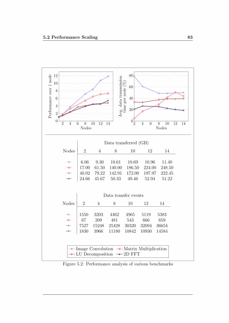
5.2 Performance Scaling 83
2 4 6 8 10 12 140
2
4
6
8
10
12
Nodes
Per
form
ance
over
1n
od
e
2 4 6 8 10 12 140
20
40
60
80
Nodes
Avg.
dat
atr
ansm
issi
onti
me
per
nod
e(%
)
Data transferred (GB)
Nodes 2 4 8 10 12 14
6.06 9.30 10.61 10.69 10.96 11.4017.00 61.50 140.00 186.50 224.00 248.5040.02 79.22 142.91 172.00 197.97 222.4524.66 45.67 50.33 49.46 52.94 51.22
Data transfer events
Nodes 2 4 8 10 12 14
1550 3203 4462 4965 5119 538367 209 481 543 666 659
7527 15248 25428 30320 32094 366541830 3966 11180 10842 10930 14584
Image Convolution Matrix MultiplicationLU Decomposition 2D FFT
Figure 5.2: Performance analysis of various benchmarks

84 Experimental Evaluation
the total experimental time in communication (of 11.4 GB), matrix multipli-
cation transfers a much larger 248.50 GB data in the cluster and this takes
43.81% of the total experimental time. Although for matrix multiplication
both input matrices are 16 GB each, every input block is required by all sub-
tasks in its row and all in its column. Thus about 250 GB data is eventually
transferred in 659 pipelined events (each of the 1024 subtasks subscribe to 1
GB data from both the input matrices).
The other two experiments, block LU decomposition and 2D-FFT, exhibit
relatively inferior scaling (4.8 and 5.36 respectively) as these experiments
have limited parallelism. The former is an iterative experiment with 32
iterations and 3 tasks per iteration (one out of these three is sequential).
The experiment has an average of 121.7 subtasks per task. The 2D-FFT
experiment (with an implicit matrix transpose operation) has two tasks each
with 120 subtasks.
The results in Figure 5.2 indicate a similar amount of data transfer for matrix
multiplication and LU decomposition. However, the former is implemented
as a single task with time complexity O(n3) and the latter has many itera-
tions with three tasks using BLAS calls of varying time complexities (O(n),
O(n2) and O(n3)). This increases communication latency, which is evident
from fifty times more data transfer events (36654 versus 659). This, coupled
with the fact that the first of these three tasks is sequential, leads to lower
scalability for the experiment. In contrast, both image convolution and 2D
FFT have lower time complexities – O(nm) for the former (m being the filter
size) and O(n log n) for the latter, but the latter has around 4.5x more data
transfer, resulting in its lower scaling. These results collectively indicate that

5.2 Performance Scaling 85
applications with high compute to communication ratio should perform well
with our runtime.
16 32 48 640
5
10
15
20
Image Dimension (x 1024)
Exec
uti
onT
ime
(in
sec)
Image Convolution
16 32 48 640
50
100
150
Matrix Dimension (x 1024)
Exec
uti
onT
ime
(in
sec)
Matrix Multiplication
4 nodes 8 nodes
Figure 5.3: Scaling with increasing problem size
Figure 5.3 plots the execution times of image convolution and matrix mul-
tiplication benchmarks with increase in the problem size. The results are
presented for two cases - in the first case only 4 cluster nodes are used for
execution while 8 cluster nodes are employed in the second case. Results
show that our runtime responds equivalently to various input sizes as similar
scaling curves (while varying workload sizes) are observed despite increase in
the number of nodes.
5.2.1 CPU versus GPU versus CPU+GPU
Figures 5.4, 5.5 and 5.6 plot GPUs-only performances for image convolu-
tion, matrix multiplication and 2D FFT respectively and compare those to
the corresponding CPU+GPU performances. For the computation in these
applications there is a significant performance disparity between CPUs and

86 Experimental Evaluation
1 2 4 8 10 12 140
20
40
60
Nodes
Exec
uti
onT
ime
(in
sec)
1 2 4 8 10 12 140
0.5
1
1.5
Nodes
%C
PU
subta
sks
Total subtasks = 1024
0
20
40
60
80
100
%G
PU
subta
sks
GPU CPU+GPU CPU GPU
Figure 5.4: Image Convolution – GPU vs. CPU+GPU
1 2 4 8 10 12 140
200
400
600
Nodes
Exec
uti
onT
ime
(in
sec)
1 2 4 8 10 12 140
2
4
6
Nodes
%C
PU
subta
sks
Total subtasks = 1024
0
20
40
60
80
100
%G
PU
subta
sks
GPU CPU+GPU CPU GPU
Figure 5.5: Matrix Multiplication – GPU vs. CPU+GPU

5.2 Performance Scaling 87
1 2 4 8 10 12 140
20
40
60
80
100
120
Nodes
Exec
uti
onT
ime
(in
sec)
1 2 4 8 10 12 140
5
10
15
20
Nodes
%C
PU
subta
sks
Total subtasks = 240
0
20
40
60
80
100
%G
PU
subta
sks
GPU CPU+GPU CPU GPU
Figure 5.6: 2D FFT – GPU vs. CPU+GPU
GPUs, with GPUs being several times faster than CPUs. Due to this, em-
ploying both together generally results in nearly all CPU subtasks getting
multi-assigned to GPUs. Also, running some subtasks on slower CPUs takes
away the opportunity to pipeline those in case the GPUs had executed them.
For these reasons, the experiments’ performances when using CPU+GPU do
not show much throughput gain over their GPUs-only versions. For image
convolution and matrix multiplication, results show that nearly 98% subtasks
were executed by GPUs and CPUs were only able to complete fewer than 2%
of the subtasks. For 2D FFT, this ratio is a little better with around 15%
subtasks completed by CPUs.
Figure 5.7 compares CPUs-only and GPUs-only performances for matrix
multiplication and 2D FFT for input matrices of size 32768 × 32768. The
wide performance disparity between CPUs and GPUs is evident in these
results (especially for matrix multiplication where in the 1-node case CPUs-
only performance is around 5 times slower than GPUs-only performance).

88 Experimental Evaluation
The disparity is narrower for 2D-FFT, where the best results occur when
using both CPUs and GPUs together. However, this experiment uses only
32 subtasks, thus restricting parallelism and performance gains to 32 devices
(i.e., 2 nodes) only. Ideally, the number of subtasks should be a few times
the number of devices. But in this case, the number of subtasks becomes less
than the number of devices as the number of nodes in the cluster grows.
1 2 4 6 8 100
100
200
300
400
500
Nodes
Exec
uti
onT
ime
(sec
s)
Matrix Multiplication
1 2 4 6 8 100
10
20
30
40
Nodes
Exec
uti
onT
ime
(sec
s)2D FFT
CPU GPU CPU+GPU
Figure 5.7: Experiments with matrices of size 32768×32768 (lower is better)
5.2.2 PageRank
Figure 5.8 presents results for the PageRank experiment. The experiment
executes 25 map-reduce iterations. In the map stage, 250 subtasks process
an equal share of input web pages and distribute their page ranks equally
among all their outlinks. In the reduce stage, the page rank contributions
from each subtask are summed up to compute the final page ranks of all
web pages. For efficiency, reductions are performed in parallel on all cluster
nodes. Once the intra-node reductions complete, nodes perform inter-node
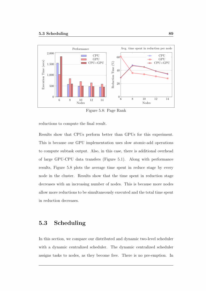
5.3 Scheduling 89
6 8 10 12 140
500
1,000
1,500
2,000
Nodes
Exec
uti
onT
ime
(sec
s)
Performance
CPUGPU
CPU+GPU
6 8 10 12 140
20
40
60
Nodes
Red
uct
ion
Tim
e(%
)
Avg. time spent in reduction per node
CPUGPU
CPU+GPU
Figure 5.8: Page Rank
reductions to compute the final result.
Results show that CPUs perform better than GPUs for this experiment.
This is because our GPU implementation uses slow atomic-add operations
to compute subtask output. Also, in this case, there is additional overhead
of large GPU-CPU data transfers (Figure 5.1). Along with performance
results, Figure 5.8 plots the average time spent in reduce stage by every
node in the cluster. Results show that the time spent in reduction stage
decreases with an increasing number of nodes. This is because more nodes
allow more reductions to be simultaneously executed and the total time spent
in reduction decreases.
5.3 Scheduling
In this section, we compare our distributed and dynamic two-level scheduler
with a dynamic centralized scheduler. The dynamic centralized scheduler
assigns tasks to nodes, as they become free. There is no pre-emption. In
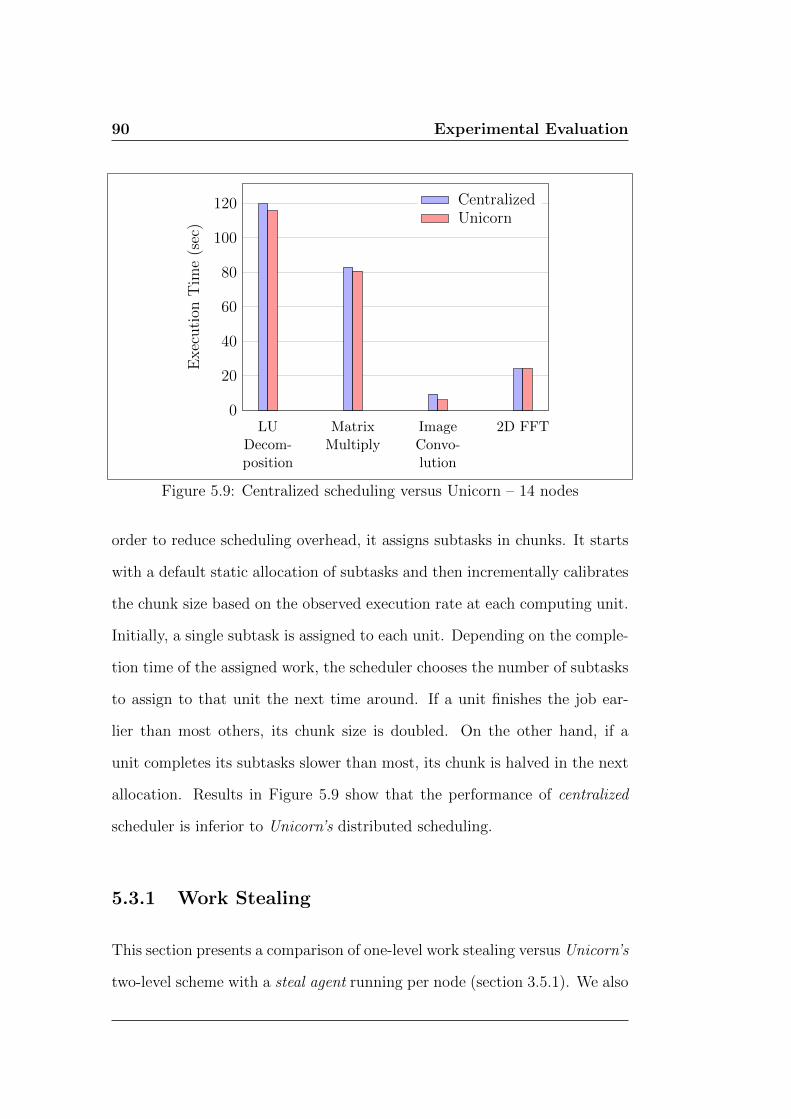
90 Experimental Evaluation
LUDecom-position
MatrixMultiply
ImageConvo-lution
2D FFT0
20
40
60
80
100
120E
xec
uti
onT
ime
(sec
)CentralizedUnicorn
Figure 5.9: Centralized scheduling versus Unicorn – 14 nodes
order to reduce scheduling overhead, it assigns subtasks in chunks. It starts
with a default static allocation of subtasks and then incrementally calibrates
the chunk size based on the observed execution rate at each computing unit.
Initially, a single subtask is assigned to each unit. Depending on the comple-
tion time of the assigned work, the scheduler chooses the number of subtasks
to assign to that unit the next time around. If a unit finishes the job ear-
lier than most others, its chunk size is doubled. On the other hand, if a
unit completes its subtasks slower than most, its chunk is halved in the next
allocation. Results in Figure 5.9 show that the performance of centralized
scheduler is inferior to Unicorn’s distributed scheduling.
5.3.1 Work Stealing
This section presents a comparison of one-level work stealing versus Unicorn’s
two-level scheme with a steal agent running per node (section 3.5.1). We also

5.3 Scheduling 91
compare the performance of the latter to our aggressive stealing scheme called
ProSteal.
5.3.1.1 One-level vs. Two-level
Results in Figure 5.10 show comparable performance numbers for one-level
and two-level scheduling schemes for matrix multiplication and LU decompo-
sition. However, image convolution and 2D FFT respectively report 6.92%
and 2.13% performance improvement with two-level stealing, compared to
the one-level stealing scheme. The gain in image convolution is because of
the small memory footprint of an image convolution subtask, which allows
GPUs (which are the stealers in most cases) to co-execute more subtasks as
compared to other experiments where despite stealing a set of subtasks large
memory footprint prohibits their co-execution.
Despite moderate performance gains, two-level stealing reports significant re-
duction (over one-level) in the total number of steals attempts generated in
the cluster. The average reduction for image convolution, matrix multiplica-
tion, LU decomposition and 2D FFT respectively is 65.88%, 64.9%, 67.03%
and 66%. Due to this, the average number of successful steals in the cluster
increase in two-level scheme (over one-level) by 44.24%, 54.25%, 60.08% and
52.3% for these experiments respectively. The same is not translated into
performance gains because our steals are extremely light weight. The only
information transferred as a result of steal is the subtask id and there is no
associated direct data transfer.

92 Experimental Evaluation
Execution time (sec) versus nodes
1 2 4 8 10 12 140
20
40
60
80
Exec
uti
onT
ime
(sec
s)
Image Convolution
1 2 4 8 10 12 140
200
400
600
Exec
uti
onT
ime
(sec
s)
Matrix Multiplication
1 2 4 8 10 12 140
200
400
600
Exec
uti
onT
ime
(sec
s)
LU Decomposition
1 2 4 8 10 12 140
50
100
Exec
uti
onT
ime
(sec
s)2D FFT
Total and successful steals (as % of total steals) versus nodes
1 2 4 8 10 12 140
1
2
Tot
alst
eals
(x10
00)
Image Convolution
0
20
40
60
Succ
essf
ul
stea
ls(%
)
1 2 4 8 10 12 140
1
2
Tot
alst
eals
(x10
00)
Matrix Multiplication
0
20
40
60
Succ
essf
ul
stea
ls(%
)
1 2 4 8 10 12 140
20
40
60
80
Tot
alst
eals
(x10
00)
LU Decomposition
0
20
40
60
Succ
essf
ul
stea
ls(%
)
1 2 4 8 10 12 140
1
2
3
4
Tot
alst
eals
(x10
00)
2D FFT
0
20
40
60
80
Succ
essf
ul
stea
ls(%
)
One-level Two-level One-level Two-level
Figure 5.10: One-level versus two-level work stealing

5.3 Scheduling 93
Execution time (sec) versus nodes
1 2 4 8 10 12 140
20
40
60
80
Nodes
Exec
uti
onT
ime
(sec
s)
Image Convolution
1 2 4 8 10 12 140
200
400
600
Nodes
Exec
uti
onT
ime
(sec
s)
LU Decomposition
Total Steals versus nodes
1 2 4 8 10 12 140
200
400
600
Nodes
Tot
alSte
als
Image Convolution
1 2 4 8 10 12 140
10,000
20,000
30,000
Nodes
Tot
alSte
als
LU Decomposition
without ProSteal with ProSteal
Successful GPU pipeline continuations
GPU pipeline continuations (% of successful GPU steals))
Nodes 1 2 4 8 10 12 14
Image Convolution 100.00 85.71 94.44 96.97 100.00 95.83 94.34LU Decomposition 81.82 74.67 66.08 61.12 59.06 55.51 58.78
Figure 5.11: Work Stealing – with and without ProSteal

94 Experimental Evaluation
5.3.1.2 ProSteal
Unicorn avoids GPU pipeline stalls by allowing devices to steal before their
pipelines are completely flushed. As discussed in chapter 3, the appropriate
time when a GPU should steal is dynamically computed based on the GPU’s
subtask execution rate and its latency to re-prime its pipeline after a stall.
Figure 5.11 plots the performance of this scheme versus the performance
obtained by Unicorn scheduler without ProSteal. On an average, ProSteal
yields 5.11% better performance for image convolution but degrades by 4%
for LU decomposition experiment. The performance gain in image convo-
lution is because ProSteal is able to avert GPU pipeline stalls for 95.33%
successful GPU steals (which are 33% of the total steals). The number is
only 65.29% for LU decomposition where successful GPU steals are only 14%
of the total steals. More detailed results of ProSteal can be found in [3].
5.3.2 Locality-aware Scheduling
In this section, we study node-affinity based scheduling in Unicorn. For this,
we have modified our experiments such that there is no particular spatial
coherence between consecutive subtasks’ data. In other words, adjacent sub-
tasks of our experiments do not necessarily execute on adjacent address space
regions.
For locality-aware scheduling, we compute an affinity score for every subtask
on every node and our scheduler uses this score to maximize global affinity.
We experiment with four heuristics. We start with scheduling a subtask on a
node where most of its input resides, maximizing local data. In this case, the

5.3 Scheduling 95
more the amount of local data (on a node) for a subtask is, the more the cor-
responding affinity score is. The other strategies, instead of maximizing local
data, target the time to fetch remote data. The next strategy minimizes the
number of remote data transfer events or requests. It is based on the observa-
tion that the incurred data fetch latency grows with data fragmentation and
the number of data transfer requests. Accessing closely placed remote data
is less expensive than accessing discontiguous remote data, which may cost
additional latency. The third strategy optimizes the amount of remote data.
It minimizes the total number of virtual memory pages to be fetched from
remote nodes. Our last strategy, called Hybrid or Derived Affinity optimizes
for both remote transfer events and time.
Figures 5.12 and 5.13 plot the performance of Unicorn’s locality-oblivious
scheduler as well as the performance of the local data based affinity and
compares these to remote data based affinity (transfer events, remote data
and hybrid). The figures also record the cluster-wide data transfers and
subtask latency incurred in these experiments.
Results show that one or more of our heuristics perform better than Unicorn’s
locality oblivious scheduler at most of the data points. For image convolution
experiment, a maximum gain of 13.93% (over Unicorn’s default scheduler) is
observed with remote data and hybrid heuristics in the fourteen node case.
This is attributed to a substantial data transfer reduction from 11.44 GB (for
default scheduler) to 0.43 GB (for remote data heuristic) and 0.78 GB (for
hybrid heuristic). A gain of similar magnitude is not reflected in execution
time because of the high throughput of our network (32 Gbps).
For the matrix multiplication experiment, we observe the maximum gain
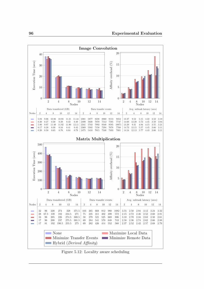
96 Experimental Evaluation
Image Convolution
2 4 8 10 12 140
10
20
30
40
Nodes
Exec
uti
onT
ime
(sec
s)
2 4 8 10 12 140
5
10
15
20
Nodes
Affi
nit
yov
erhea
d(%
)Data transferred (GB) Data transfer events Avg. subtask latency (secs)
Nodes 2 4 8 10 12 14 2 4 8 10 12 14 2 4 8 10 12 14
5.94 9.06 10.86 10.93 11.21 11.44 2381 5877 8238 8860 9113 9454 13.37 9.52 5.15 4.22 3.52 3.100.20 0.27 0.30 0.39 0.43 0.49 2499 5020 7070 7512 7595 7747 14.69 12.29 5.73 4.45 3.58 3.045.80 9.97 11.49 11.92 11.90 12.11 2241 5743 7992 9348 9595 10071 13.29 9.31 4.94 4.15 3.55 3.210.17 0.28 0.30 0.34 0.41 0.43 2369 5502 7158 7294 7678 7768 14.73 12.15 5.57 4.45 3.66 3.110.20 0.50 0.65 0.76 0.84 0.78 2475 5410 7015 7348 7493 7801 14.54 12.13 5.77 4.43 3.66 3.11
Matrix Multiplication
2 4 8 10 12 140
100
200
300
400
500
Nodes
Exec
uti
onT
ime
(sec
s)
2 4 8 10 12 140
5
10
15
20
Nodes
Affi
nit
yov
erhea
d(%
)
Data transferred (GB) Data transfer events Avg. subtask latency (secs)
Nodes 2 4 8 10 12 14 2 4 8 10 12 14 2 4 8 10 12 14
32 96 220 274 328 371.5 103 265 668 812 980 1082 3.55 2.50 2.94 3.12 3.24 3.3228 67.5 139 182 234.5 271 75 235 311 402 499 572 2.15 2.72 2.46 2.52 2.60 2.8116 96 205 226 274.5 308.5 58 279 521 525 669 806 3.10 2.70 2.34 2.63 2.50 2.6117 96 208 237 275.5 301.5 69 284 541 570 648 743 2.58 2.36 2.74 2.62 2.66 2.8817 81 192 190.5 255.5 275 69 282 426 414 552 568 2.37 2.52 2.42 2.57 2.68 2.79
None Maximize Local DataMinimize Transfer Events Minimize Remote DataHybrid (Derived Affinity)
Figure 5.12: Locality aware scheduling

5.3 Scheduling 97
LU Decomposition
2 4 8 10 12 140
100
200
300
400
500
600
Nodes
Exec
uti
onT
ime
(sec
s)
2 4 8 10 12 140
1
2
3
4
Nodes
Affi
nit
yov
erhea
d(%
)
Data transferred (GB) Data transfer events Avg. subtask latency (secs)
Nodes 2 4 8 10 12 14 2 4 8 10 12 14 2 4 8 10 12 14
105.99 179.77 255.39 281.45 303.30 322.33 21430 33845 40047 43163 44561 45819 5.16 4.05 3.32 3.18 3.07 2.9543.08 87.66 131.84 154.25 164.89 177.13 6856 13489 17115 18496 18271 18871 4.47 3.83 3.37 3.15 3.01 2.8841.42 100.48 161.80 182.17 196.86 214.28 7739 16042 23579 23321 23901 24499 4.48 3.78 3.31 3.10 2.96 2.8840.23 109.98 162.64 191.77 211.63 224.97 7097 17919 22386 25628 25539 26173 4.40 3.84 3.37 3.19 2.94 2.9337.28 91.28 144.06 160.61 184.00 198.97 6938 14250 19639 18889 21543 21715 4.42 3.75 3.37 3.11 2.99 2.85
2D FFT
2 4 8 10 12 140
20
40
60
80
Nodes
Exec
uti
onT
ime
(sec
s)
2 4 8 10 12 140
2
4
6
8
10
Nodes
Affi
nit
yov
erhea
d(%
)
Data transferred (GB) Data transfer events Avg. subtask latency (secs)
Nodes 2 4 8 10 12 14 2 4 8 10 12 14 2 4 8 10 12 14
23.12 41.63 49.22 50.62 52.02 52.35 6333 16540 24168 27885 30425 32174 3.04 2.90 3.23 3.32 3.44 3.7220.84 30.47 25.55 26.48 31.87 36.49 1515 9305 3772 4919 12535 17548 2.51 2.94 3.69 3.56 3.56 3.8522.41 33.75 25.32 25.78 28.12 29.41 1771 10450 3277 3594 7170 9615 3.34 3.23 3.63 3.73 3.39 3.7122.64 31.77 24.61 25.79 28.36 29.16 1604 10111 1841 3628 7689 8893 3.28 3.32 3.55 3.65 3.51 3.7322.28 29.79 25.55 25.55 28.36 30.35 1205 8368 4049 3062 7583 9802 3.31 3.39 3.55 3.56 3.52 3.71
None Maximize Local DataMinimize Transfer Events Minimize Remote DataHybrid (Derived Affinity)
Figure 5.13: Locality aware scheduling (Contd.)

98 Experimental Evaluation
of 21.94% in the two node case with the hybrid heuristic. This result is
attributed to a 88.24% reduction in data transfer, a 49.28% reduction in
data transfer events and a 1.18 sec gain in average subtask latency. Note
that this is a communication bound experiment and the reduction in data
transfer has resulted in a large gain in performance. However, there is an
observed overhead of 16.42% in affinity computation.
For the LU decomposition experiment, the hybrid heuristic performs better
than others at most of the data points and we observe an average gain of 8.6%
with this heuristic. On an average, this heuristic results in a 45.37% reduction
in total data transfer and has a reported average overhead of 2.21%. The
experiment has moderate performance gains as compared to data transfer
savings as it is an iterative experiment, with a mix of compute and commu-
nication bound tasks per iteration.
The 2D FFT experiment does not gain much by affinity as the savings in
data transfer are mitigated by high affinity computation overheads. The
maximum gain for this experiment is observed with transfer events heuristic
which, in the fourteen node case, yields a speed-up of 2.8% after accounting
for 9.31% affinity computation overhead.
Among all our heuristics, the derived affinity scheme gives close to the best
results (at most data points). The overhead of computing and using affinity
is non-trivial, though. The results suggest that employing other methods
of affinity computation (e.g. taking affinity as input from application or
augmenting address space directory with affinity data all the time) might
help in making the heuristics more useful. Further study on affinity and its
overhead can be found in [4].
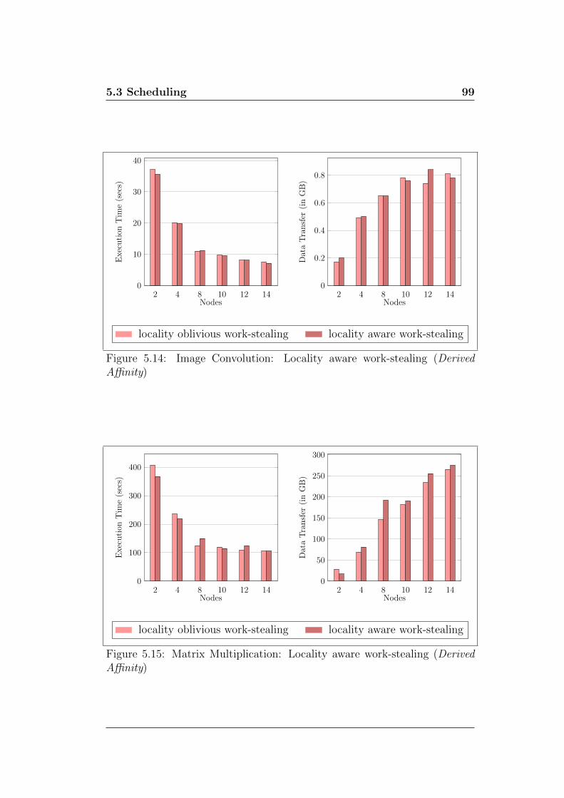
5.3 Scheduling 99
2 4 8 10 12 140
10
20
30
40
Nodes
Exec
uti
onT
ime
(sec
s)
2 4 8 10 12 140
0.2
0.4
0.6
0.8
NodesD
ata
Tra
nsf
er(i
nG
B)
locality oblivious work-stealing locality aware work-stealing
Figure 5.14: Image Convolution: Locality aware work-stealing (DerivedAffinity)
2 4 8 10 12 140
100
200
300
400
Nodes
Exec
uti
onT
ime
(sec
s)
2 4 8 10 12 140
50
100
150
200
250
300
Nodes
Dat
aT
ransf
er(i
nG
B)
locality oblivious work-stealing locality aware work-stealing
Figure 5.15: Matrix Multiplication: Locality aware work-stealing (DerivedAffinity)

100 Experimental Evaluation
Our runtime also uses the computed affinity information while work stealing.
We let the victim assign those subtasks to the stealer that are high on affinity
scores for the stealer but low on affinity scores for the victim. Figures 5.14
and 5.15 plot performance numbers of locality oblivious work-stealing versus
locality aware work-stealing for the derived affinity heuristic. For the image
convolution experiment, we observe an average performance gain of 1.74%
while the matrix multiplication experiment reports a flat response on an
average with locality aware work-stealing (as compared to locality oblivious
work-stealing). We do not observe much improvement with locality-aware
work-stealing primarily because by the time stealing happens most of the
subtasks have already executed and secondly because we use stale affinity
information (computed at task start) for work-stealing and do not update
this as the task progresses (see section 3.5.1.2.2).
5.4 Load Balancing
In this section, we study the effectiveness of our scheduler in achieving a
balanced load on all cluster devices. Figures 5.16 and 5.17 respectively plot
the finishing times of all cluster devices for the image convolution benchmark
and for one iteration of the PageRank experiment. The figures also plot the
number of subtasks executed by each of these devices. Note that all the
CPU devices on a node are represented as work-groups numbered from W1
to W14. Similarly, GPU devices in the cluster are labelled G1 to G28.
Recall that for the matrix multiplication experiment, the entire input data
is initially equally distributed randomly among all cluster nodes. For this

5.4 Load Balancing 101
reason, all GPUs execute roughly the same number of subtasks (as they face
similar data transfer overheads and subtasks are homogeneous). The same is
true for CPU work-groups. For the PageRank experiment, however, the input
data is resident on NFS. The graph plots 10th iteration of the experiment
which means that the input data for the iteration additionally comes from
different cluster nodes (as it is computed in last iteration). As such, variable
input data latency is incurred by various CPU work-groups, causing them
to execute different number of subtasks. Despite the disparity in subtask
execution rate of GPUs and CPU work-groups, the finishing times of each of
them is quite close to each other (for both experiments). This shows that our
scheduler is able to balance the cluster load despite this device heterogeneity.
In another experiment (matrix multiplication on 10 nodes using GPUs only),
we study the effectiveness of our load balancer (Figure 5.18) in the centralized
initial data placement scheme (section 5.5.2). Since the entire data is located
on the first node, our runtime schedules more subtasks on the two GPUs of
this node as compared to the others. Since all 20 GPUs in the cluster finish
at roughly the same time, load balance can be inferred.
W1
G1
G2
W2
G3
G4
W3
G5
G6
W4
G7
G8
W5
G9
G10
W6
G11
G12
W7
G13
G14
W8
G15
G16
W9
G17
G18
W10
G19
G20
W11
G21
G22
W12
G23
G24
W13
G25
G26
W14
G27
G28
0
20
40
1 2 3 4 5 6 7 8 9 10 11 12 13 14Node
Device
Subta
sks
Exec
ute
d
W1
G1
G2
W2
G3
G4
W3
G5
G6
W4
G7
G8
W5
G9
G10
W6
G11
G12
W7
G13
G14
W8
G15
G16
W9
G17
G18
W10
G19
G20
W11
G21
G22
W12
G23
G24
W13
G25
G26
W14
G27
G28
0
5
10
Tim
e(s
ecs)
Subtasks Completed Subtasks Canceled Running Time
Figure 5.16: Load Balancing (Image Convolution) – W denotes a CPU workgroup and G denotes a GPU device – Block random data distribution

102 Experimental Evaluation
W1
G1
G2
W2
G3
G4
W3
G5
G6
W4
G7
G8
W5
G9
G10
W6
G11
G12
W7
G13
G14
W8
G15
G16
W9
G17
G18
W10
G19
G20
W11
G21
G22
W12
G23
G24
W13
G25
G26
W14
G27
G28
0
5
10
15
20
1 2 3 4 5 6 7 8 9 10 11 12 13 14Node
Device
Subta
sks
Exec
ute
d
W1
G1
G2
W2
G3
G4
W3
G5
G6
W4
G7
G8
W5
G9
G10
W6
G11
G12
W7
G13
G14
W8
G15
G16
W9
G17
G18
W10
G19
G20
W11
G21
G22
W12
G23
G24
W13
G25
G26
W14
G27
G28
0
50
100
150
200
Tim
e(s
ecs)
Subtasks Completed Subtasks Canceled Running Time
Figure 5.17: Load Balancing (Page Rank) – W denotes a CPU work groupand G denotes a GPU device
1 2 3 4 5 6 7 8 9 10111213141516171819200
10
20
1 2 3 4 5 6 7 8 9 10NodeGPU
Subta
sks
Exec
ute
d
1 2 3 4 5 6 7 8 9 10111213141516171819200
10
20
Tim
e(s
ecs)
Subtasks Completed Subtasks Canceled Running Time
Figure 5.18: Load Balancing (Matrix Multiplication) – 32768× 32768 matri-ces – Centralized data distribution
5.5 Stress Tests
In this section, we put our runtime under non-favorable conditions and study
its response to various experiments. We study three things – firstly the re-
sponse of our runtime when subtasks in the image convolution experiment are
made to execute subtasks of different sizes, secondly the impact of changing
the input data availability pattern before start of the experiment and thirdly

5.5 Stress Tests 103
the impact of changing the size of subtasks employed in the experiment.
5.5.1 Heterogeneous Subtasks
W1
G1
G2
W2
G3
G4
W3
G5
G6
W4
G7
G8
W5
G9
G10
W6
G11
G12
W7
G13
G14
W8
G15
G16
W9
G17
G18
W10
G19
G20
0
20
40
1 2 3 4 5 6 7 8 9 10Node
Device
Subta
sks
Exec
ute
d
W1
G1
G2
W2
G3
G4
W3
G5
G6
W4
G7
G8
W5
G9
G10
W6
G11
G12
W7
G13
G14
W8
G15
G16
W9
G17
G18
W10
G19
G20
0
5
10
15
20
Tim
e(s
ecs)
Subtasks Completed Subtasks Canceled Running Time
Figure 5.19: Load Balancing (Heterogeneous Subtasks) – W denotes a CPUwork group and G denotes a GPU device
Figure 5.19 shows load balancing achieved by Unicorn when subtasks in
Image Convolution experiment perform different amount of work. The top
half of the image is convolved using 512 subtasks of size 2048 × 2048 while
the bottom half is convolved using 128 subtasks of size 4096 × 4096. The
experiment is executed on 10 nodes. Despite, the four fold execution disparity
in subtasks, our runtime maintains a decent load balance in the cluster.
5.5.2 Input Data Distributions
In this section, we vary the placement of the initial input data in the address
space(s). Figure 5.20 evaluates image convolution and matrix multiplication
for various schemes like centralized (entire address space on one cluster node),
row random (rows of 2048×2048 blocks placed randomly on all cluster nodes),

104 Experimental Evaluation
2 4 6 8 10 12 140
1
2
3
4
Nodes
TF
lop
/s
Image Convolution
2 4 6 8 10 12 140
2
4
6
NodesT
Flo
p/s
Matrix Multiplication
Centralized Row random Column random Block random
Row random for first matrix and column random for second
Figure 5.20: Impact of initial data distribution pattern
column random (columns of 2048×2048 blocks placed randomly on all cluster
nodes) and block random (2048×2048 blocks placed randomly on any cluster
node). Additionally, a fifth scheme is plotted for matrix multiplication where
rows of 2048× 2048 blocks for the first input matrix and columns of 2048×
48 blocks for the second input matrix are placed randomly in the cluster.
Results show that our runtime maintains performance despite the changes
in data availability pattern. Only the centralized scheme behaves poorly
as the network interface of the node containing the entire data becomes a
bottleneck.
5.5.3 Varying Subtask Size
Figure 5.21 shows the response of our runtime to change in user’s sizing of
subtask. Within a reasonable range – (2048-8192) for matrix multiplication
and (1024-4096) for image convolution – our system is able to maintain a

5.6 Unicorn Optimizations 105
0 1 2 3 4 5 6 7 8 9
Imag
eC
onvo
-lu
tion
Mat
rix
Mult
iply
#Subtasks = []
[16384][4096][1024][256][64]
[64][256]
[1024][4096]
[16384]
TFlop/s
N 512 10242048 4096 8192
Figure 5.21: Subtask size (N ×N) – experiments executed on 14 nodes
throughput within 20% of the peak performance. On either side, system
overheads begin to dominate. For extreme sizes, the throughput degrades
as on one extreme there are too few subtasks to generate enough parallelism
and on the other there are too many subtasks resulting in data transfers
dominating the exploitable parallelism.
5.6 Unicorn Optimizations
In this section, we study the impact of two major Unicorn optimizations –
multi-assign and pipelining. We study the overhead of multi-assign along with
its performance benefits. This is followed by a study of performance gains
achieved by creating a pipeline of subtasks, which enables communications
of a few subtasks be overlapped with computations of others.

106 Experimental Evaluation
5.6.1 Multi-Assign
1 2 4 8 10 12 140
20
40
60
Nodes
Exec
uti
onT
ime
(sec
)
Image Convolution
1 2 4 8 10 12 140
200
400
600
Nodes
Exec
uti
onT
ime
(sec
)
Matrix Multiplication
without multi-assign with multi-assign
Figure 5.22: Multi-Assign (no external load)
15 x 15 23 x 23 31 x 310
100
200
300
Filter Size (n x n)
Exec
uti
onT
ime
(sec
)
without multi-assignwith multi-assign
Figure 5.23: Multi-assign under external load (Image Convolution) – 4 nodes
We study two cases to understand the implications of multi-assign. First,
under the absence of any external load we compare the performance of image
convolution and matrix multiplication experiments with multi-assign enabled

5.6 Unicorn Optimizations 107
to the case with multi-assign disabled. Second, we create an external load
and study how image convolution behaves with and without multi-assign.
For the first case, results in Figure 5.22 show that there is no performance
penalty in enabling multi-assign, in general. The observed average perfor-
mance gain (with multi-assign) for image convolution and matrix multipli-
cation respectively are 9.19% and 2.23% respectively (in comparison to no
multi-assign). In fact, the performance gains increase with increasing num-
ber of nodes – for image convolution, multi-assign reports a maximum gain
of 38.26% (over no multi-assign) in the fourteen node case. Similarly, the
maximum performance gain of 10.62% is observed in the fourteen node case
for matrix multiplication.
Next, we study multi-assignment over four nodes with the image convolution
benchmark. We artificially overload one of the nodes with one process per
core computing trigonometric functions indefinitely. In this case, we expect
subtasks assigned to the overloaded node to be moved away from it. Our
scheduler does this through stealing and multi-assignment. In the absence
of multi-assignment a subtask may start running on a slow device and take
a long time to finish, thereby, delaying the entire task. We run this test
twice: once allowing multi-assignment and once preventing it. Results in
Figure 5.23 show that with multi-assignment, subtasks of the overloaded
cores get re-assigned and the task completes faster. Without it, the task
remains bottlenecked by the ‘slow’ cores. Our heuristics generally only multi-
assign fewer than 1% of the subtasks, but the later-assigned unit finishes
first about 50% of the time. Of course, when one finishes, the other is
aborted, leading to a faster overall time. The cancellation protocol itself has

108 Experimental Evaluation
insignificant overhead.
5.6.2 Pipelining
1 2 4 8 10 12 140
50
100
150
200
250
Nodes
Exec
uti
onT
ime
(sec
)
without pipeliningwith pipelining
Figure 5.24: Pipelining (Image Convolution)
Figure 5.24 shows the impact of pipelining with the help of the image con-
volution experiment. With pipelining, our runtime overlaps computation of
one subtask with the communication of the next. Further, on GPUs this
makes multiple simultaneous kernel executions possible. Results show that
our runtime achieves 3-4x speed-up with pipelining.
In [2], we study pipelining for an experimental 10-node cluster and report
its effectiveness in hiding remote data access latency. If all required data
were locally available on each of the 10 nodes, image convolution gets only
1% faster and matrix multiplication gets 31% faster. On the other hand,
disabling pipelining makes them 2.29x and 1.19x slower, respectively.

5.6 Unicorn Optimizations 109
5.6.3 Software cache for GPUs
2 4 6 8 10 12 140
2
4
6
Nodes
TF
lop
/s
Performance
2 4 6 8 10 12 140.2
0.22
0.24
0.26
0.28
0.3
0.32
Nodes
Byte
sev
icte
d/a
lloca
ted
Avg. evictions per allocation
LRU MRU LFU MFU Random No Cache
1 2 4 8 10 12 140
500
1,000
Nodes
Cac
he
Mis
ses
Avg. cache misses per GPU
LRU MRU LFU MFU Random
Figure 5.25: Matrix Multiplication – GPU Cache Eviction Strategies
Unicorn employs a software cache to reduce DMA data transfers to all GPUs
in the cluster. The cache prevents read-only data shared by two or more

110 Experimental Evaluation
subtasks (of a task) executing on a GPU from being DMA’ed more than
once. The cache also prevents data transfers in case a write-only or read-
write data generated by a subtask is later consumed by a subtask of another
task.
In this section, we study four cache eviction policies and compare their per-
formances. The four policies are least recently used (which evicts the data of
subtask that was used the earliest in time), most recently used (which evicts
the data of subtask that was used the latest in time), least frequently used
(which evicts the data of subtask that was used the minimum number of
times) and most frequently used (which evicts the data of subtask that was
used the maximum number of times). Figure 5.25 plots the performances of
these policies where these are respectively denoted by shorthand notations
LRU, MRU, LFU and MFU. Results show that both LRU and LFU per-
form better than MRU and MFU. This result can also be inferred from lesser
number of cache evictions per allocation and lesser number of average cache
misses in LRU and LFU as compared to MRU and MFU.
5.6.4 Data Compression
To ameliorate high data transfer latency in PageRank reduction, we compress
data computed by subtasks before transferring over the network or from GPU
to CPU. The employed compression algorithm is based on Run Length En-
coding (section 10.1) and is executed on GPUs for GPU→CPU data trans-
fers and on CPUs for inter-node data transfers. Figure 5.26 presents the
cluster-wide size of uncompressed data (i.e. before compression) for reduc-
tion, compression ratio (i.e. the ratio of uncompressed size to compressed

5.7 Overhead Analysis 111
size) and performance boost with compression (over the case when there is
no compression). Results show that the performance gains increase with
increase in the number of nodes and reach a peak of 23.81% for network
compression and a peak of 2.45% for GPU→CPU compression (for the 14
node case). Note that because of lower latency of GPU→CPU transfers, the
gain observed with GPU compression is moderate as compared to inter-node
compression. Also, note that the amount of data transferred in the cluster
increases with the number of nodes. However, this reduces the number of
subtasks processed per node which means that inter-node reductions take
place with more sparsity in data (and thus higher compression yield).
Network reduction statistics GPU→CPU reduction statisticsNodes Uncompressed Compression Performance Uncompressed Compression Performance
Data Size (GB) Ratio Gain (%) Data Size (GB) Ratio Gain (%)
8 162.98 3.63 6.44 27.01 44.63 0.3110 209.55 4.72 16.10 25.15 44.64 0.8312 256.11 5.29 21.00 23.28 44.66 0.6414 302.68 5.78 23.81 31.67 44.61 2.45
Figure 5.26: PageRank data compression (250 million web pages)
5.7 Overhead Analysis
In this section, we evaluate the overhead of our implementation of Unicorn’s
runtime firstly by varying the number of CPU cores used in the experiments
and secondly by studying the amount of time experiments spend inside run-
time’s code versus the application code.

112 Experimental Evaluation
2 4 6 8 10 12 140
1
2
3
4
Nodes
TF
lop
/s
Image Convolution
2 4 6 8 10 12 140
2
4
6
NodesT
Flo
p/s
Matrix Multiplication
7 cores 8 cores 9 cores10 cores 11 cores 12 cores
Figure 5.27: Varying CPU cores used in subtask computation
5.7.1 Varying CPU cores
CPU cores are not only used for subtask computations but for many other
critical operations like CPU-GPU data transfers, network data transfers,
scheduling and Unicorn runtime’s control operations. For all our experi-
ments presented in this section, we have reserved two CPU cores (out of 12
available) per node for these support functions and presented results by using
the rest for subtask computations. Figure 5.27 varies the number of CPU
cores allowed for the application subtasks per node from 7 to 12 and compares
their performances. Results show that the performance of all these cases re-
main close to each other. The average difference between the maximum and
minimum performing cases (at all data points) for both experiments is less
than 10%.
This narrow performance difference is an indication of our runtime’s low

5.7 Overhead Analysis 113
overhead. Because of this low overhead, we currently do not dynamically
vary the number of CPU cores used in a Unicorn task. An exploration of
this is desired in future. However, we currently do allow applications to
statically specify the number of CPU cores to be reserved for a task.
2 4 6 8 10 12 140
2
4
6
Nodes
TF
lop
/s
10 cores
[0:0] [2:0] [1:1]
2 4 6 8 10 12 140
2
4
6
Nodes
TF
lop
/s
8 cores
[0:0] [4:0] [2:2]
Figure 5.28: Matrix Multiplication – Varying CPU core affinity
We also study the impact of binding our compute threads (section 3) to
CPU cores. In all the experiments presented thus far, we have not explicitly
bound compute threads to processing cores, allowing the operating system
to manage them. Figure 5.28 compares this scenario to the case when all
our compute threads are explicitly bound to CPU cores (which leaves a few
cores for other critical operations like data transfers). The figure plots the
performance of the matrix multiplication experiment for two cases - when 10
cores and 8 cores are employed in subtask computation. For each case, we
report performance when there is no explicit core for these critical operations
(plotted as [0:0]). Relative to this, we plot performances of cases where
[n:m] cores are designated for non-subtask computations (i.e. n cores are

114 Experimental Evaluation
explicitly freed from first CPU while m cores are explicitly freed from the
second one). Results show that explicit binding of compute threads (to cores)
does not have a significant performance impact. However, not explicitly
binding threads and letting the operating system to freely migrate them
yields best performance.
5.7.2 Unicorn Time versus Application Time
1 2 4 8 10 12 140
20
40
60
Nodes
Applica
tion
Tim
e(s
ec)
Image Convolution
0
0.2
0.4
0.6
Unic
orn
Tim
e(se
c)
1 2 4 8 10 12 140
200
400
600
Nodes
Applica
tion
Tim
e(s
ec)
Matrix Multiplication
0
0.5
1
1.5
Unic
orn
Tim
e(s
ec)
Application time Unicorn time
Figure 5.29: Library time versus application time
Figure 5.29 compares the time spent (by image convolution and matrix mul-
tiplication experiments) in runtime’s code to the time spent in application
execution. The latter includes the time taken for data transfers (both net-
work and CPU-GPU) and callback executions. The rest of the experimental
time is considered as our runtime’s overhead. Results show that the aver-
age overhead for image convolution is 3.6% while it is 0.91% for the matrix
multiplication experiment. In absolute value, the average overhead is 0.43
seconds for image convolution and 0.82 seconds for matrix multiplication.

5.7 Overhead Analysis 115
5.7.3 Data Transfer Frequency
Image Convolution Matrix MultiplicationAvg. unique Avg. total Avg. transfer Avg. unique Avg. total Avg. transfer Avg. first matrix
Nodes data sent per data sent per freq. per byte data sent per data sent per freq. per byte transfer freq. per
node (GB) node (GB) per node node (GB) node (GB) per node byte per node
2 3.05 3.05 1.00 8.50 8.50 1.00 1.004 2.26 2.27 1.00 7.38 15.88 2.15 1.188 1.31 1.32 1.01 5.63 18.19 3.23 1.8610 1.07 1.07 1.01 4.50 18.20 4.04 2.1712 0.91 0.92 1.01 4.00 18.83 4.71 2.7814 0.87 0.88 1.01 3.18 18.36 5.78 2.88
Figure 5.30: Data Transfer Frequency
In this section, we study the number of times each byte in the address space
gets transferred in the cluster (between nodes). Two examples are consid-
ered – on one end is the image convolution experiment which has very little
subscription overlap (fringe) among subtasks. At the other end is matrix
multiplication where entire input data of every subtask overlaps with that
of other subtasks. Figure 5.30 lists the average number of unique and total
bytes transferred by every node in the cluster along with the average data
transfer frequency (i.e., the ratio of total bytes transferred to unique bytes
transferred per node). Results show that the data transfer frequency stays
close to 1 for the image convolution experiment, whereas it grows with in-
creasing number of nodes for the matrix multiplication experiment. This is
because one of input matrices is required on all cluster nodes and because
of the initial random placement of data, (n-1) transfers are required (where
n is the number of nodes). The other matrix, however, exhibits relatively
moderate transfer frequency (the last column in the table).
Most of the data transferred is only because it resides at a node different from

116 Experimental Evaluation
the subtask that requires it. For matrix multiplication, e.g., disabling steal-
ing and multi-assignment reduces the unique data sent per node by 5.88% on
average. Correspondingly, the total data sent and transfer frequency per byte
decrease by 9.76% and 4.97% respectively. Thus, there is only 3.88% addi-
tional transfer due to re-sending of data to the new destination after stealing
or multi-assignment. The rest 96.12% data transfer is due to subscription
overlap among subtasks.
5.8 Unicorn versus others
Figure 5.31 compares the performance of our matrix multiplication exper-
iment (single node) to StarPU [6]. The three bars for StarPU plot, re-
spectively, its default eager scheduler, the first run of its advanced dmdas
scheduler (i.e., without calibration; this scheduler requires calibration runs
for optimal performance), and the best run out of three successive runs of
dmdas after calibration. This best run performs better than Unicorn until
a matrix size of 16384× 16384. For larger matrices, it starts to lag Unicorn
and eventually fails at 65536 × 65536 reporting it ran out of memory. Yet,
Unicorn runs at this and even higher sizes.
Figure 5.32 compares Unicorn to SUMMA[58] for multiplication of two square
matrices (on CPUs only) of size 32768 × 32768. Results show that Unicorn
performs quite close to SUMMA (which is hand tuned for matrix multiplica-
tion) for this double precision computation. Note that SUMMA incurs a bit
of overhead in the sense that it requires a different MPI process per CPU core
whereas Unicorn works with one MPI process per node. For this experiment,

5.8 Unicorn versus others 117
4096 8192 163840
5
10
Square Matrix Dimension
Exec
uti
onT
ime
(sec
)
32768 40960 49152 57344 655360
200
400
600
Square Matrix Dimension
Exec
uti
onT
ime
(sec
)
eager dmdas (pre-calibration) dmdas (calibrated) Unicorn
Figure 5.31: Unicorn versus StarPU
2 4 5 8 100
200
400
600
800
1,000
Nodes
Exec
uti
onT
ime
(sec
)
SUMMA Unicorn
Figure 5.32: Unicorn versus SUMMA
118 Experimental Evaluation
we have used different block sizes for both implementations (1024× 1024 for
Unicorn and 128 × 128 for SUMMA) in order to compare their best CPU
performances.

Chapter 6
Application Profiling
1 Pa r a l l e l Task 6 Execution Time = 15.7919 [ Schedul ing Po l i cy : WS]
2 Subtask d i s t r i b u t i o n f o r task [ 0 , 1 ] . . .
3 Device Subtask Execution P r o f i l e . . .4 Device 0 Subtasks 45 Device 12 Subtasks 1086 Device 13 Subtasks 567 Device 14 Subtasks 38 Device 26 Subtasks 909 Device 27 Subtasks 75
10 Machine Subtask Execution P r o f i l e . . .11 Machine 0 Subtasks 168 CPU Subtasks 412 Machine 1 Subtasks 168 CPU Subtasks 3
13 Total Acknowledgements Received 336
14 Address Space [ 0 , 1 ] memory t r a n s f e r s t a t i s t i c s on [ Host 0 ] . . .15 1235888826 bytes memory r e c e i v ed in 155 events16 1236443811 bytes memory t r a n s f e r r e d in 163 events
17 Address Space [ 0 , 2 ] memory t r a n s f e r s t a t i s t i c s on [ Host 0 ] . . .18 0 bytes memory r e c e i v ed in 0 events19 0 bytes memory t r a n s f e r r e d in 0 events
Figure 6.1: Sample Unicorn Logs (part 1)
Unicorn provides compile time controls for profiling various modules of the
library. The resultant logs help identify application and runtime bottle-
necks. Among others, the logs dump address space allocations and their
data transfers across cluster nodes, work-stealing and multi-assign statistics,
task and subtask execution timeline, MPI calls issued at each cluster node,
node affinity statistics, load balancing and scheduling information. The logs
are dumped out in textual format like the ones in figures 6.1, 6.2 and 6.3.
Logs in Figure 6.1 show the total experimental time taken under the default
work stealing scheduling policy and the number of subtasks executed by each

120 Application Profiling
1 Task P r o f i l e r [ Host 0 ] . . . . . . . . . . . .
2 INPUTMEMORYTRANSFER => Accumulated Time : 20515.3 s ; Actual Time =6.86013 s ; Overlapped Time = 20508.4 s
3 OUTPUTMEMORYTRANSFER => Accumulated Time : 0 s ; Actual Time = 0 s ;Overlapped Time = 0 s
4 TOTALMEMORYTRANSFER => Accumulated Time : 20517.9 s ; Actual Time =6.86123 s ; Overlapped Time = 20511.1 s
5 DATA PARTITIONING => Accumulated Time : 0 .406627 s ; Actual Time =0.376811 s ; Overlapped Time = 0.0298162 s
6 SUBTASK EXECUTION => Accumulated Time : 137.482 s ; Actual Time =15.324 s ; Overlapped Time = 122.158 s
7 DATAREDUCTION => Accumulated Time : 0 s ; Actual Time = 0 s ;Overlapped Time = 0 s
8 DATA REDISTRIBUTION => Accumulated Time : 0 s ; Actual Time = 0 s ;Overlapped Time = 0 s
9 MEMORYCOMMIT => Accumulated Time : 0 s ; Actual Time = 0 s ;Overlapped Time = 0 s
10 SUBTASK STEAL WAIT => Accumulated Time : 8 .32788 s ; Actual Time =6.59817 s ; Overlapped Time = 1.72971 s
11 SUBTASK STEAL SERVE => Accumulated Time : 0 .000205755 s ; Actual Time= 0.000205755 s ; Overlapped Time = 0 s
12 STUBWAITONNETWORK => Accumulated Time : 8 .46128 s ; Actual Time =4.97415 s ; Overlapped Time = 3.48713 s
13 COPYTOPINNEDMEMORY => Accumulated Time : 0 .700807 s ; Actual Time= 0.663236 s ; Overlapped Time = 0.037571 s
14 COPYFROMPINNEDMEMORY => Accumulated Time : 1 .1685 s ; Actual Time= 1.1685 s ; Overlapped Time = 0 s
15 CUDACOMMANDPREPARATION => Accumulated Time : 0 .00107765 s ; ActualTime = 0.00107765 s ; Overlapped Time = 0 s
16 UNIVERSAL => Accumulated Time : 20679.8 s ; Actual Time = 15.3001 s ;Overlapped Time = 20664.5 s
Figure 6.2: Sample Unicorn Logs (part 2)
machine and device (CPU/GPU) in the cluster. The figure also shows the
amount of memory sent or received (and the number of send/receive events)
for every address space used on a node in the cluster.
Figure 6.2 shows the work done (Accumulated Time) and the wall clock time
spent (Actual Time) in various events like memory transfers, data subscrip-
tion, stealing, copy to/from pinned buffers, etc. The work done is the arith-
metic sum of the times spent by various threads while the wall clock time
accounts for the time overlapped between these threads only once. The com-
mon time between threads is displayed under the heading Overlapped Time.
Figure 6.3 shows the cumulative memory transfers (across all address spaces)
for a task on a node. Beneath that, the subtask execution rate for each stub

121
1 Task Exec Stat s [ Host 0 ] . . . . . . . . . . . .
2 Memory Trans f e r s Received = 1235888826 bytes ; Receive Events =155 ; Sent = 1236443811 bytes ; Send Events = 163
3 Scat te r ed Memory Trans f e r s Received = 1235888826 bytes ; ReceiveEvents = 155 ; Sent = 1236443811 bytes ; Send Events = 163
4 Device 0 Subtask execut ion ra t e = 0 .0386306 ; S t ea l attempts = 2 ;Su c c e s s f u l s t e a l s = 0 ; Fa i l ed s t e a l s = 2 ; P i p e l i n e s a c r o s sranges = 0
5 Device 12 Subtask execut ion ra t e = 7 . 05162 ; S t ea l attempts = 3 ;Su c c e s s f u l s t e a l s = 1 ; Fa i l ed s t e a l s = 2 ; P i p e l i n e s a c r o s sranges = 1
6 Device 13 Subtask execut ion ra t e = 4 . 1 3 1 ; S t ea l attempts = 2 ;Su c c e s s f u l s t e a l s = 0 ; Fa i l ed s t e a l s = 2 ; P i p e l i n e s a c r o s sranges = 0
7 Unicorn [ Host 0 ] Event Timel ine Device 08 Task [ 0 , 1 ] Subtask 281 ( Sp l i t 0 o f 12) 41 .2708 43.85839 Task [ 0 , 1 ] Subtask 281 Event SubtaskExecution 41.4977 43 .85810 Task [ 0 , 1 ] Subtask 281 Event WaitOnNetwork 41.2789 41 .49711 Task [ 0 , 1 ] Subtask 325 ( Sp l i t 0 o f 12) 43 .8586 46 .79712 Task [ 0 , 1 ] Subtask 325 Event SubtaskExecution 44.2574 46.796713 Task [ 0 , 1 ] Subtask 325 Event WaitOnNetwork 43 .942 44.2572
14 Unicorn [ Host 0 ] Event Timel ine Device 1215 Task [ 0 , 1 ] Subtask 11 43.1959 44.767316 Task [ 0 , 1 ] Subtask 11 Event CopyFromPinnedMemory 44.6632 44.766917 Task [ 0 , 1 ] Subtask 11 Event CopyToPinnedMemory 43.3631 43.366518 Task [ 0 , 1 ] Subtask 11 Event SubtaskExecution 43.3668 43.367219 Task [ 0 , 1 ] Subtask 32 43.6812 45.022920 Task [ 0 , 1 ] Subtask 32 Event CopyFromPinnedMemory 44.8802 44.884321 Task [ 0 , 1 ] Subtask 32 Event CopyToPinnedMemory 43.6829 43.686722 Task [ 0 , 1 ] Subtask 32 Event SubtaskExecution 43 .687 43.687523 Task [ 0 , 1 ] Subtask 33 41.5666 43.847224 Task [ 0 , 1 ] Subtask 33 Event CopyFromPinnedMemory 43.6878 43.846825 Task [ 0 , 1 ] Subtask 33 Event CopyToPinnedMemory 41.6809 41.684126 Task [ 0 , 1 ] Subtask 33 Event SubtaskExecution 41.6843 41.684727 Task [ 0 , 1 ] Subtask 33 Event WaitOnNetwork 41.5898 41.6744
Figure 6.3: Sample Unicorn Logs (part 3)
is reported. This is accompanied by the total number of steal attempts by a
device, the number of successful ones (out of the total) and in case the stealer
is a GPU device, the figure also reports the number of steal attempts that
were able to bring in new subtasks before the GPU pipeline stalled. Lastly,
the figure displays the event timeline, i.e., the start and end times for various
events happening on each device in the cluster. These events include subtask
execution, wait for remote data transfers, time spent in transfers to/from
pinned buffers for GPUs, etc.

122 Application Profiling
Unicorn has an analysis engine that can consume these textual logs as input
and generate easily understandable graphs. The graphs include performance
and scalability charts, CPU versus GPU versus CPU+GPU charts, load bal-
ancing, multi-assign and event timeline charts. A few sample charts are
shown in figures 6.4, 6.5, 6.6 and 6.7.
Figure 6.4 depicts the performance improvements in a sample experiment
when the number of nodes used in the cluster are increased from 2 to 10.
Figure 6.5 shows the load balance achieved by various GPUs in the cluster.
Figure 6.6 compares the centralized work-sharing scheduler (Push) described
in section 5.3 with the Unicorn’s work-stealing scheduler (Pull). In both
cases, there is a plot with compute communication overlap enabled and a
plot with this optimization disabled. Finally, Figure 6.7 shows activities of
cluster devices over a timeline during the experiment.
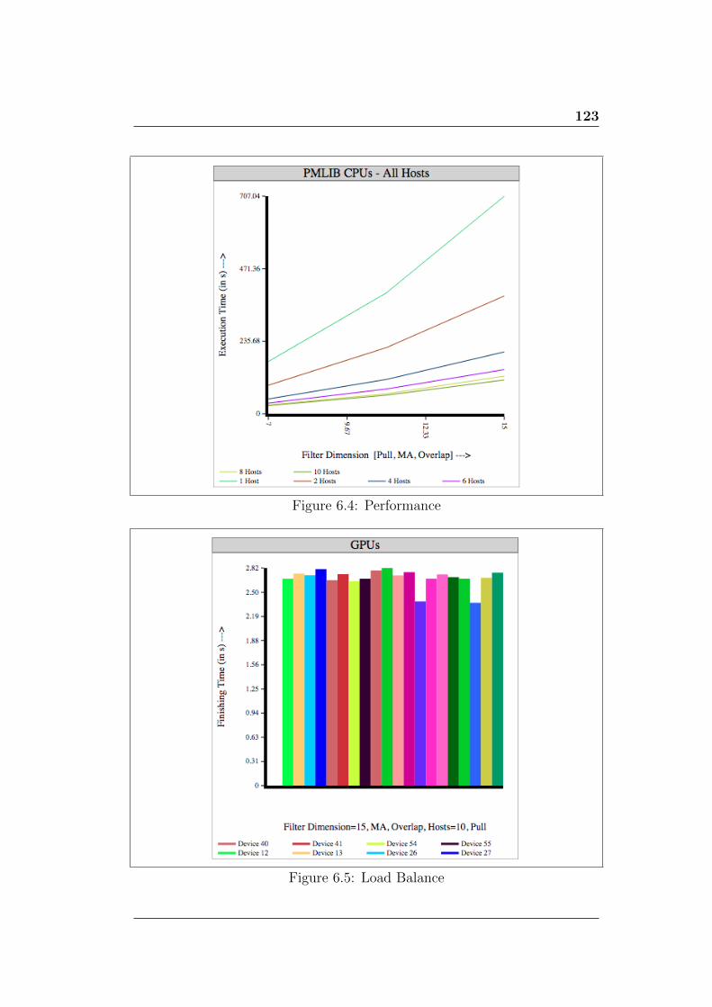
123
Figure 6.4: Performance
Figure 6.5: Load Balance
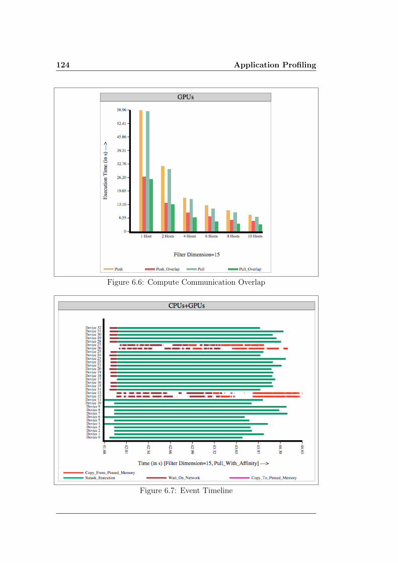
124 Application Profiling
Figure 6.6: Compute Communication Overlap
Figure 6.7: Event Timeline

Chapter 7
Public API
This section documents Unicorn’s public headers - pmPublicDefinitions.h
(Listing 7.1) and pmPublicUtilities.h (Listing 7.2). The prefix pm is taken
from code name (PMLIB which is short for Partitioned Memory Library) of
this project.
1 namespace pm2 {3 typedef unsigned short int ushort ;4 typedef unsigned int uint ;5 typedef unsigned long ulong ;
6 const s ize t MAX NAME STR LEN = 256 ;7 const s ize t MAX DESC STR LEN = 1024 ;8 const s ize t MAX CB KEY LEN = 128 ;9 const s ize t MAX MEM SECTIONS PER TASK = 8 ;
10 /∗∗11 ∗ This enumeration d e f i n e s s u c c e s s and a l l
e r r o r c o n d i t i o n s f o r the PMLIB Appl i ca t ionProgramming I n t e r f a c e (API) .
12 ∗ Appl i ca t i on s can depend upon these s t a t u sf l a g s to know the outcome o f PMLIB f u n c t i o n s .
13 ∗ Appl i ca t i on s may use pmGetLastError f o r ab r i e f d e s c r i p t i o n o f the e r r o r .
14 ∗/15 typedef enum pmStatus16 {17 pmSuccess = 0 ,18 pmOk,

126 Public API
19 pmStatusUnavailable ,20 pmFatalError ,21 p m I n i t i a l i z a t i o n F a i l u r e ,22 pmNetworkInitError ,23 pmNetworkTerminationError ,24 pmInvalidIndex ,25 pmInvalidCommand ,26 pmThreadingLibraryFailure ,27 pmTimerFailure ,28 pmMemoryError ,29 pmNetworkError ,30 pmIgnorableError ,31 pmGraphicsCardError ,32 pmBeyondComputationalLimits ,33 pmUnrecognizedMemory ,34 pmInvalidKey ,35 pmMaxKeyLengthExceeded ,36 pmDataProcessingFai lure ,37 pmNoCompatibleDevice ,38 pmConfFileNotFound ,39 pmInval idOffset ,40 pmInval idCal lbacks ,41 pmUserError ,42 pmMaxStatusValues43 } pmStatus ;
44 /∗∗ This func t i on r e tu rn s the PMLIB ' s v e r s i onnumber as a char ∗ in the formatMajorVersion MinorVersion Update ∗/
45 const char∗ pmGetLibVersion ( ) ;
46 /∗∗ This func t i on r e tu rn s a b r i e f d e s c r i p t i o n o fthe l a s t e r r o r ( i f any ) caused by execut iono f any PMLIB func t i on ∗/
47 const char∗ pmGetLastError ( ) ;
48 /∗∗ This func t i on i n i t i a l i z e s the PMLIB l i b r a r y .I t must be the f i r s t PMLIB API c a l l e d on a l lmachines under MPI c l u s t e r . ∗/
49 pmStatus p m I n i t i a l i z e ( ) ;

127
50 /∗∗ This func t i on marks the te rminat ion o f useo f PMLIB in an a p p l i c a t i o n . This must be thea p p l i c a t i o n ' s l a s t c a l l to PMLIB. ∗/
51 pmStatus pmFinal ize ( ) ;
52 /∗∗ This func t i on r e tu rn s the id o f the c a l l i n ghost ∗/
53 uint pmGetHostId ( ) ;
54 /∗∗ This func t i on r e tu rn s the t o t a l number o fhos t s ∗/
55 uint pmGetHostCount ( ) ;
56 /∗∗ Some bas i c type d e f i n i t i o n s ∗/57 typedef void∗ pmMemHandle ;58 typedef void∗ pmRawMemPtr ;59 typedef void∗ pmTaskHandle ;60 typedef void∗ pmDeviceHandle ;61 typedef void∗ pmCallbackHandle ;62 typedef void∗ pmClusterHandle ;
63 typedef enum pmMemType64 {65 READ ONLY,66 WRITE ONLY,67 READ WRITE,68 READ ONLY LAZY,69 WRITE ONLY LAZY,70 READ WRITE LAZY,71 MAX MEM TYPE72 } pmMemType;
73 typedef enum pmSubscriptionType74 {75 READ SUBSCRIPTION,76 WRITE SUBSCRIPTION,77 READ WRITE SUBSCRIPTION78 } pmSubscriptionType ;
79 typedef enum pmSubscr ip t i onVi s ib i l i tyType80 {

128 Public API
81 SUBSCRIPTION NATURAL, // D i s j o i n ts u b s c r i p t i o n s are mapped at samed i s t a n c e s as in task memory ( d e f a u l topt ion )
82 SUBSCRIPTION COMPACT, // D i s j o i n ts u b s c r i p t i o n s are mapped back to back
83 SUBSCRIPTION OPTIMAL, // Ei therSUBSCRIPTION NATURAL orSUBSCRIPTION COMPACT whichever i s opt imalf o r the subtask
84 MAX SUBSCRIPTION VISBILITY TYPE85 } pmSubscr ip t i onVi s ib i l i tyType ;
86 /∗∗ St ruc tu r e s f o r memory s u b s c r i p t i o n ∗/87 typedef struct pmSubscr ipt ionInfo88 {89 s ize t o f f s e t ; /∗ O f f s e t from the s t a r t o f
the memory reg i on ∗/90 s ize t l ength ; /∗ Number o f bytes to be
subsc r ibed ∗/
91 pmSubscr ipt ionInfo ( ) ;92 pmSubscr ipt ionInfo ( s ize t , s ize t ) ;93 } pmSubscr ipt ionInfo ;
94 typedef struct pmScatte redSubscr ipt ionIn fo95 {96 s ize t o f f s e t ;97 s ize t s i z e ;98 s ize t s tep ;99 s ize t count ;
100 pmScatte redSubscr ipt ionIn fo ( ) ;101 pmScatte redSubscr ipt ionIn fo ( s ize t , s ize t ,
s ize t , s ize t ) ;102 } pmScatte redSubscr ipt ionIn fo ;
103 /∗∗ GPU context f o r subtask ∗/104 typedef struct pmGpuContext105 {106 void∗ s c r a t c h B u f f e r ;107 void∗ reservedGlobalMem ;

129
108 pmGpuContext ( ) ;109 } pmGpuContext ;
110 /∗∗ User in fo rmat ion typede f s ∗/111 typedef struct pmSpl i t In fo112 {113 uint s p l i t I d ;114 uint sp l i tCount ;
115 pmSpl i t In fo ( ) ;116 pmSpl i t In fo ( uint , uint ) ;117 } pmSpl i t In fo ;
118 typedef struct pmMemInfo119 {120 pmRawMemPtr ptr ;121 pmRawMemPtr readPtr ;122 pmRawMemPtr wr i tePtr ;123 s ize t l ength ;124 pmSubscr ip t i onVi s ib i l i tyType v i s i b i l i t y T y p e ;
125 pmMemInfo ( ) ;126 pmMemInfo(pmRawMemPtr, pmRawMemPtr,
pmRawMemPtr, s ize t ) ;127 pmMemInfo(pmRawMemPtr, pmRawMemPtr,
pmRawMemPtr, s ize t ,pmSubsc r ip t i onVi s ib i l i tyType ) ;
128 } pmMemInfo ;
129 typedef struct pmSubtaskInfo130 {131 ulong subtaskId ;132 pmMemInfo memInfo [MAX MEM SECTIONS PER TASK ] ;133 uint memCount ;134 pmGpuContext gpuContext ;135 pmSpl i t In fo s p l i t I n f o ;
136 pmSubtaskInfo ( ) ;137 pmSubtaskInfo (ulong , pmMemInfo∗ , uint ) ;138 } pmSubtaskInfo ;

130 Public API
139 typedef struct pmTaskInfo140 {141 pmTaskHandle taskHandle ;142 void∗ taskConf ;143 uint taskConfLength ;144 ulong taskId ;145 ulong subtaskCount ;146 ushort p r i o r i t y ;147 uint o r i g i n a t i n g H o s t ;
148 pmTaskInfo ( ) ;149 } pmTaskInfo ;
150 typedef struct pmDataTransferInfo151 {152 pmMemHandle memHandle ;153 s ize t memLength ;154 s ize t ∗ operatedMemLength ; // Mem Length
a f t e r programmer ' s compress ion / encrypt ion155 pmMemType memType ;156 uint srcHost ;157 uint destHost ;
158 pmDataTransferInfo ( ) ;159 } pmDataTransferInfo ;
160 typedef enum pmDeviceType161 {162 CPU = 0 ,163 #i f d e f SUPPORT CUDA164 GPU CUDA,165 #e n d i f166 MAX DEVICE TYPES167 } pmDeviceType ;
168 typedef struct pmDeviceInfo169 {170 pmDeviceHandle deviceHandle ;171 char name [MAX NAME STR LEN ] ;172 char d e s c r i p t i o n [MAX DESC STR LEN ] ;173 pmDeviceType deviceType ;174 uint host ;

131
175 uint deviceIdOnHost ;176 uint dev i c e Id InC lu s t e r ;
177 pmDeviceInfo ( ) ;178 } pmDeviceInfo ;
179 typedef enum pmSchedul ingPol icy180 {181 SLOW START,182 RANDOM STEAL, /∗ d e f a u l t p o l i c y ∗/183 RANDOM STEAL WITH AFFINITY,184 EQUAL STATIC,185 PROPORTIONAL STATIC,186 NODE EQUAL STATIC187 } pmSchedul ingPol icy ;
188 typedef enum pmAf f in i tyCr i t e r i on189 {190 MAXIMIZE LOCAL DATA,191 MINIMIZE REMOTE SOURCES,192 MINIMIZE REMOTE TRANSFER EVENTS,193 MINIMIZE REMOTE TRANSFERS ESTIMATED TIME,194 DERIVED AFFINITY,195 MAX AFFINITY CRITERION196 } pmAf f in i tyCr i t e r i on ;
197 /∗ The l i f e t i m e o f s c ra t ch b u f f e r f o r a subtask∗/
198 typedef enum pmScratchBufferType199 {200 PRE SUBTASK TO SUBTASK, // Scratch
b u f f e r l i v e s from data d i s t r i b u t i o nc a l l b a c k to subtask c a l l b a c k
201 SUBTASK TO POST SUBTASK, // Scractchb u f f e r l i v e s from subtask c a l l b a c k todata r e d i s t r i b u t i o n / reduct i on c a l l b a c k
202 PRE SUBTASK TO POST SUBTASK, // Scratchb u f f e r l i v e s from data d i s t r i b u t i o nc a l l b a c k to data r e d i s t r i b u t i o n / reduct i onc a l l b a c k
203 REDUCTION TO REDUCTION // Scratchb u f f e r l i v e s and t r a v e l s from one data

132 Public API
r educt i on c a l l b a c k to the next ( evena c ro s s machines )
204 } pmScratchBufferType ;
205 typedef struct pmRedistr ibutionMetadata206 {207 uint order ;208 uint count ;
209 pmRedistr ibutionMetadata ( ) ;210 pmRedistr ibutionMetadata ( uint , uint ) ;211 } pmRedistributionMetadata ;
212 /∗∗ The f o l l o w i n g type d e f i n i t i o n s stand f o r thec a l l b a c k s implemented by the user programs . ∗/
213 typedef pmStatus(∗ pmDataDistr ibut ionCal lback ) ( pmTaskInfopTaskInfo , pmDeviceInfo pDeviceInfo ,pmSubtaskInfo pSubtaskInfo ) ;
214 typedef pmStatus(∗ pmSubtaskCallback CPU ) ( pmTaskInfopTaskInfo , pmDeviceInfo pDeviceInfo ,pmSubtaskInfo pSubtaskInfo ) ;
215 typedef void(∗pmSubtaskCallback GPU CUDA ) ( pmTaskInfopTaskInfo , pmDeviceInfo∗ pDeviceInfo ,pmSubtaskInfo pSubtaskInfo , pmStatus∗pStatus ) ; // po in t e r to CUDA kerne l
216 typedef pmStatus(∗ pmSubtaskCallback GPU Custom ) ( pmTaskInfopTaskInfo , pmDeviceInfo pDeviceInfo ,pmSubtaskInfo pSubtaskInfo , void∗pCudaStream ) ;
217 typedef pmStatus(∗ pmDataReductionCallback ) ( pmTaskInfopTaskInfo , pmDeviceInfo pDevice1Info ,pmSubtaskInfo pSubtask1Info , pmDeviceInfopDevice2Info , pmSubtaskInfo pSubtask2Info ) ;
218 typedef pmStatus(∗ pmDataRedistr ibutionCal lback ) ( pmTaskInfopTaskInfo , pmDeviceInfo pDeviceInfo ,

133
pmSubtaskInfo pSubtaskInfo ) ;219 typedef bool
(∗ pmDeviceSe lect ionCal lback ) ( pmTaskInfopTaskInfo , pmDeviceInfo pDeviceIn fo ) ;
220 typedef pmStatus(∗ pmPreDataTransferCallback ) ( pmTaskInfopTaskInfo , pmDataTransferInfopDataTrans fer Info ) ;
221 typedef pmStatus(∗ pmPostDataTransferCallback ) ( pmTaskInfopTaskInfo , pmDataTransferInfopDataTrans fer Info ) ;
222 typedef pmStatus(∗ pmTaskCompletionCallback ) ( pmTaskInfopTaskInfo ) ;
223 /∗∗ Uni f i ed c a l l b a c k s t r u c t u r e ∗/224 typedef struct pmCallbacks225 {226 pmDataDistr ibut ionCal lback da taD i s t r i bu t i on ;227 pmSubtaskCallback CPU subtask cpu ;228 pmSubtaskCallback GPU CUDA subtask gpu cuda ;229 pmSubtaskCallback GPU Custom
subtask gpu custom ; // At l ea s t one o fsubtask gpu cuda and subtask gpu custommust be NULL
230 pmDataReductionCallback dataReduction ;231 pmDataRedistr ibutionCal lback
dataRed i s t r i bu t i on ;232 pmDeviceSe lect ionCal lback d e v i c e S e l e c t i o n ;233 pmPreDataTransferCallback preDataTransfer ;234 pmPostDataTransferCallback postDataTransfer ;235 pmTaskCompletionCallback
taskComplet ionCal lback ;236 const char∗ subtask openc l ;
237 pmCallbacks ( ) ;238 pmCallbacks ( pmDataDistr ibutionCal lback ,
const char∗ subtask openc l ) ;239 pmCallbacks ( pmDataDistr ibutionCal lback ,
const char∗ subtask openc l ,pmDataReductionCallback ) ;

134 Public API
240 pmCallbacks ( pmDataDistr ibutionCal lback ,const char∗ subtask openc l ,pmDataRedistr ibutionCal lback ) ;
241 pmCallbacks ( pmDataDistr ibutionCal lback ,pmSubtaskCallback CPU ,pmSubtaskCallback GPU CUDA ) ;
242 pmCallbacks ( pmDataDistr ibutionCal lback ,pmSubtaskCallback CPU ,pmSubtaskCallback GPU Custom ) ;
243 pmCallbacks ( pmDataDistr ibutionCal lback ,pmSubtaskCallback CPU ,pmSubtaskCallback GPU CUDA ,pmDataReductionCallback ) ;
244 pmCallbacks ( pmDataDistr ibutionCal lback ,pmSubtaskCallback CPU ,pmSubtaskCallback GPU Custom ,pmDataReductionCallback ) ;
245 pmCallbacks ( pmDataDistr ibutionCal lback ,pmSubtaskCallback CPU ,pmSubtaskCallback GPU CUDA ,pmDataRedistr ibutionCal lback ) ;
246 pmCallbacks ( pmDataDistr ibutionCal lback ,pmSubtaskCallback CPU ,pmSubtaskCallback GPU Custom ,pmDataRedistr ibutionCal lback ) ;
247 } pmCallbacks ;
248 /∗∗ The c a l l b a c k r e g i s t e r a t i o n API . Thec a l l b a c k s must be r e g i s t e r e d on a l l machinesus ing the same key .
249 ∗ The r e g i s t e r e d c a l l b a c k s are returned in thepo in t e r pCallbackHandle ( i f r e g i s t e r a t i o n i ss u c c e s s f u l ) .
250 ∗/251 pmStatus pmRegisterCal lbacks ( const char∗ pKey ,
pmCallbacks pCallbacks , pmCallbackHandle∗pCallbackHandle ) ;
252 /∗ The r e g i s t e r e d c a l l b a c k s must be r e l e a s e d bythe a p p l i c a t i o n us ing the f o l l o w i n g API ∗/
253 pmStatus pmReleaseCal lbacks ( pmCallbackHandlepCallbackHandle ) ;

135
254 /∗∗ The memory c r e a t i o n API . The a l l o c a t e dmemory i s returned in the v a r i a b l e pMemHandle∗/
255 pmStatus pmCreateMemory ( s ize t pLength ,pmMemHandle∗ pMemHandle) ;
256 /∗∗ The 2D memory c r e a t i o n API . The a l l o c a t e dmemory i s returned in the v a r i a b l e pMemHandle .
257 ∗ The a l l o c a t e d memory has a two dimens iona llayout with pRows rows and pCols columns .
258 ∗/259 pmStatus pmCreateMemory2D( s ize t pRows , s ize t
pCols , pmMemHandle∗ pMemHandle) ;
260 /∗ The memory d e s t r u c t i o n API . The samei n t e r f a c e i s used f o r both input and outputmemory ∗/
261 pmStatus pmReleaseMemory (pmMemHandle pMemHandle) ;
262 /∗∗ This rou t in e reads the e n t i r e d i s t r i b u t e dmemory pointed to by pMem from the e n t i r ec l u s t e r i n to the l o c a l b u f f e r . This i s ab lock ing c a l l .
263 ∗/264 pmStatus pmFetchMemory(pmMemHandle pMemHandle) ;
265 /∗∗ This rou t in e f e t c h e s pLength bytes o fd i s t r i b u t e d memory pointed to by pMem fromo f f s e t pOf f s e t i n to the l o c a l b u f f e r . This i sa b lock ing c a l l .
266 ∗/267 pmStatus pmFetchMemoryRange (pmMemHandle
pMemHandle , s ize t pOffset , s ize t pLength ) ;
268 /∗∗ This rou t in e r e tu rn s the naked memorypo in t e r a s s o c i a t e d with pMem handle .
269 ∗ This po in t e r may be used in memcpy andr e l a t e d f u n c t i o n s .
270 ∗/271 pmStatus pmGetRawMemPtr(pmMemHandle pMemHandle ,
pmRawMemPtr∗ pPtr ) ;

136 Public API
272 /∗∗ The memory s u b s c r i p t i o n APIs . Thesee s t a b l i s h memory dependenc ies f o r a subtask .
273 ∗ Any subtask i s not a l lowed to sub s c r i b e onbeha l f any other subtask .
274 ∗ These func t i on can only be c a l l e d fromDataDis t r ibut ion c a l l b a c k . The e f f e c t
275 ∗ o f c a l l i n g t h i s f unc t i on otherwi s e i sundef ined . The f u n c t i o n s can be mixed in
276 ∗ any order and may be c a l l e d mul t ip l e t imesf o r a p a r t i c u l a r subtask .
277 ∗/278 pmStatus pmSubscribeToMemory ( pmTaskHandle
pTaskHandle , pmDeviceHandle pDeviceHandle ,ulong pSubtaskId , pmSpl i t In fo& pSp l i t I n f o ,uint pMemIndex , pmSubscriptionTypepSubscriptionType , const pmSubscr ipt ionInfo&pSubsc r i p t i on In f o ) ;
279 pmStatus pmSubscribeToMemory ( pmTaskHandlepTaskHandle , pmDeviceHandle pDeviceHandle ,ulong pSubtaskId , pmSpl i t In fo& pSp l i t I n f o ,uint pMemIndex , pmSubscriptionTypepSubscriptionType , constpmScatte redSubscr ipt ionIn fo&pS ca t t e r e dSu bs c r i p t i on In f o ) ;
280 /∗∗ The memory r e d i s t r i b u t i o n API . I te s t a b l i s h e s memory orde r ing f o r an
281 ∗ address space computed by a subtask in thef i n a l task memory . Order 0 i s assumed
282 ∗ to be the f i r s t order . Data f o r order 1 i sp laced a f t e r a l l data f o r order 0 .
283 ∗ There i s no guaranteed orde r ing i n s i d e anorder number i f mu l t ip l e subtasks
284 ∗ produce data f o r that order . This func t i oncan only be c a l l e d from DataRed i s t r ibut ion
285 ∗ c a l l b a c k . The e f f e c t o f c a l l i n g t h i sfunc t i on otherw i s e i s undef ined .
286 ∗/287 pmStatus pmRedistributeData ( pmTaskHandle
pTaskHandle , pmDeviceHandle pDeviceHandle ,

137
ulong pSubtaskId , pmSpl i t In fo& pSp l i t I n f o ,uint pMemIndex , s ize t pOffset , s ize tpLength , uint pOrder ) ;
288 /∗∗ The CUDA launch c o n f i g u r a t i o n s t r u c t u r e ∗/289 typedef struct pmCudaLaunchConf290 {291 int blocksX ;292 int blocksY ;293 int blocksZ ;294 int threadsX ;295 int threadsY ;296 int threadsZ ;297 int sharedMem ;
298 pmCudaLaunchConf ( ) ;299 pmCudaLaunchConf ( int , int , int , int , int ,
int ) ;300 pmCudaLaunchConf ( int , int , int , int , int ,
int , int ) ;301 } pmCudaLaunchConf ;
302 /∗∗ The CUDA launch c o n f i g u r a t i o n s e t t i n g API .I t s e t s k e rne l launch c o n f i g u r a t i o n f o r thesubtask s p e c i f i e d by
303 ∗ pSubtaskId . The launch c o n f i g u r a t i o n i ss p e c i f i e d in the s t r u c t u r e pCudaLaunchConf .
304 ∗ This func t i on can only be c a l l e d fromDataDis t r ibut ion c a l l b a c k . The e f f e c t
305 ∗ o f c a l l i n g t h i s f unc t i on otherwi s e i sundef ined .
306 ∗/307 pmStatus pmSetCudaLaunchConf ( pmTaskHandle
pTaskHandle , pmDeviceHandle pDeviceHandle ,ulong pSubtaskId , pmSpl i t In fo& pSp l i t I n f o ,pmCudaLaunchConf& pCudaLaunchConf ) ;
308 /∗∗ I f subtask gpu custom i s set , a p p l i c a t i o nmay need to a l l o c a t e a CUDA b u f f e r in thecustom c a l l b a c k .
309 ∗ cudaMalloc and l i k e f u n c t i o n s aresynchronous and they i n t e r r u p t any

138 Public API
p o s s i b i l i t y o f asynchronous launches ,310 ∗ r e s u l t i n g in l i m i t e d occupancy on the
dev i ce . By us ing t h i s funct ion , a subtaskcan upfront ask the l i b r a r y
311 ∗ to r e s e r v e that b u f f e r . This b u f f e r can beacce s s ed in k e r n e l s us ingpSubtaskInfo . gpuContext→ reservedGlobalMem
312 ∗ This func t i on can only be c a l l e d fromDataDis t r ibut ion c a l l b a c k . The e f f e c t o fc a l l i n g t h i s func t i on otherw i se
313 ∗ i s undef ined .314 ∗/315 pmStatus pmReserveCudaGlobalMem ( pmTaskHandle
pTaskHandle , pmDeviceHandle pDeviceHandle ,ulong pSubtaskId , pmSpl i t In fo& pSp l i t I n f o ,s ize t pSize ) ;
316 /∗∗ The s t r u c t u r e that a s s o c i a t e s ta sk s toaddress spaces ∗/
317 typedef struct pmTaskMem318 {319 pmMemHandle memHandle ;320 pmMemType memType ;321 pmSubscr ip t i onVi s ib i l i tyType
s u b s c r i p t i o n V i s i b i l i t y T y p e ; /∗ Byde fau l t , t h i s i s SUBSCRIPTION NATURAL ∗/
322 bool di s jo intReadWritesAcrossSubtasks ; /∗By de fau l t , t h i s i s f a l s e . Appl ies onlyto RW adre s s spaces . ∗/
323 pmTaskMem( ) ;324 pmTaskMem(pmMemHandle , pmMemType) ;325 pmTaskMem(pmMemHandle , pmMemType,
pmSubscr ip t i onVi s ib i l i tyType ) ;326 pmTaskMem(pmMemHandle , pmMemType,
pmSubscr ipt ionVis ib i l i tyType , bool ) ;327 } pmTaskMem;
328 /∗∗ The task d e t a i l s s t r u c t u r e used f o r tasksubmiss ion ∗/
329 typedef struct pmTaskDetails330 {

139
331 void∗ taskConf ;332 uint taskConfLength ;333 pmTaskMem∗ taskMem ;334 uint taskMemCount ;335 pmCallbackHandle ca l lbackHandle ;336 ulong subtaskCount ;337 ulong taskId ; /∗ Meant f o r a p p l i c a t i o n to
a s s i g n and i d e n t i f y ta sk s ∗/338 ushort p r i o r i t y ; /∗ By de fau l t , t h i s i s
s e t to max p r i o r i t y l e v e l (0 ) ∗/339 pmSchedul ingPol icy p o l i c y ; /∗ By de fau l t ,
t h i s i s SLOW START ∗/340 int timeOutInSecs ; /∗ By de fau l t , t h i s i s
max p o s s i b l e va lue in s igned int ,negat ive va lue s mean no timeout ∗/
341 bool multiAssignEnabled ; /∗ By de fau l t ,t h i s i s t rue ∗/
342 bool overlapComputeCommunication ; /∗ Byde fau l t , t h i s i s t rue ∗/
343 bool canSpl itCpuSubtasks ; /∗ By de fau l t ,t h i s i s f a l s e ∗/
344 bool canSpl itGpuSubtasks ; /∗ By de fau l t ,t h i s i s f a l s e ∗/
345 #i f d e f SUPPORT CUDA346 bool cudaCacheEnabled ; /∗ By de fau l t , t h i s
i s t rue ∗/347 #e n d i f348 bool suppressTaskLogs ; /∗ By de fau l t , t h i s
i s f a l s e ∗/349 pmAf f in i tyCr i t e r i on a f f i n i t y C r i t e r i o n ; /∗
By de fau l t , t h i s i s MAXIMIZE LOCAL DATA ∗/350 pmClusterHandle c l u s t e r ; /∗ Unused ∗/
351 pmTaskDetails ( ) ;352 pmTaskDetails ( void∗ taskConf , uint
taskConfLength , pmTaskMem∗ , uinttaskMemCount , pmCallbackHandlecal lbackHandle , ulong subtaskCount ) ;
353 } pmTaskDetails ;
354 /∗ The f l a g d i s jo intReadWritesAcrossSubtasksshould be t rue ( f o r RW output memories ) i f

140 Public API
the read s u b s c r i p t i o n s o f a subtask do notover lap with wr i t e s u b s c r i p t i o n s o f anysubtasks other than i t s e l f . ∗/
355 /∗∗ The task submiss ion API . Returns the taskhandle in v a r i a b l e pTaskHandle on s u c c e s s . ∗/
356 pmStatus pmSubmitTask ( pmTaskDetailspTaskDetai ls , pmTaskHandle∗ pTaskHandle ) ;
357 /∗∗ The submitted ta sk s must be r e l e a s e d by thea p p l i c a t i o n us ing the f o l l o w i n g API .
358 ∗ The API automat i ca l l y b locks t i l l taskcomplet ion . Returns the task ' s e x i t s t a t u s .
359 ∗/360 pmStatus pmReleaseTask ( pmTaskHandle pTaskHandle ) ;
361 /∗∗ A task i s by d e f a u l t non b lock ing . Thec o n t r o l comes back immediately .
362 ∗ Use the f o l l o w i n g API to wait f o r the taskto f i n i s h .
363 ∗ The API r e tu rn s the e x i t s t a t u s o f the task .364 ∗/365 pmStatus pmWaitForTaskCompletion ( pmTaskHandle
pTaskHandle ) ;
366 /∗∗ Returns the task execut ion time ( in seconds )in the v a r i a b l e pTime .
367 ∗ The API automat i ca l l y b locks t i l l taskcomplet ion .
368 ∗/369 pmStatus
pmGetTaskExecutionTimeInSecs ( pmTaskHandlepTaskHandle , double∗ pTime) ;
370 /∗∗ A u n i f i e d API to r e l e a s e task and i t ' sa s s o c i a t e d r e s o u r c e s ( ca l l back s , input andoutput memory) .
371 ∗ Returns the task ' s e x i t s t a t u s ( i f noe r r o r ) . The API automat i ca l l y b locks t i l ltask f i n i s h e s .
372 ∗/373 pmStatus pmReleaseTaskAndResources ( pmTaskDetails

141
pTaskDetai ls , pmTaskHandle pTaskHandle ) ;
374 /∗∗ This func t i on r e tu rn s a wr i t ab l e b u f f e ra c c e s s i b l e to data d i s t r i b u t i o n , subtask ,data reduct i on and data r e d i s t r i b u t i o nc a l l b a c k s .
375 Scratch b u f f e r s i z e parameter i s only honoredf o r the f i r s t i nvoca t i on o f t h i s func t i onf o r a p a r t i c u l a r subtask and sc ra t ch b u f f e rtype .
376 Succ e s s i v e i n v o c a t i o n s re turn the b u f f e ra l l o c a t e d at i n i t i a l r eque s t s i z e . Thisb u f f e r i s only used to pass in fo rmat iongenerated in one c a l l b a c k
377 to other c a l l b a c k s ∗/378 #i f d e f CUDACC379 h o s t d e v i c e380 #e n d i f381 inl ine void∗ pmGetScratchBuffer ( pmTaskHandle
pTaskHandle , pmDeviceHandle pDeviceHandle ,ulong pSubtaskId , pmSpl i t In fo& pSp l i t I n f o ,pmScratchBufferType pScratchBufferType ,s ize t pBuf f e rS i ze , pmGpuContext∗ pGpuContext )
382 {383 #i f de f ined ( CUDA ARCH )384 return ( pGpuContext ?
pGpuContext→ s c r a t c h B u f f e r : NULL) ;385 #else386 void∗
pmGetScratchBufferHostFunc ( pmTaskHandlepTaskHandle , pmDeviceHandlepDeviceHandle , ulong pSubtaskId ,pmSpl i t In fo& pSp l i t I n f o ,pmScratchBufferType pScratchBufferType ,s ize t pBuf f e rS i z e ) ;
387 returnpmGetScratchBufferHostFunc ( pTaskHandle ,pDeviceHandle , pSubtaskId , pSp l i t I n f o ,pScratchBufferType , pBu f f e rS i z e ) ;
388 #e n d i f389 }

142 Public API
390 /∗∗ This func t i on i s only supported from CPU andcan not be c a l l e d from GPU k e r n e l s ∗/
391 pmStatus pmReleaseScratchBuf fer ( pmTaskHandlepTaskHandle , pmDeviceHandle pDeviceHandle ,ulong pSubtaskId , pmSpl i t In fo& pSp l i t I n f o ,pmScratchBufferType pScratchBufferType ) ;
392 /∗∗ This func t i on r e tu rn s theREDUCTION TO REDUCTION sc ra t ch b u f f e ra s s o c i a t e d with the f i n a l reduced subtask o fthe task pTaskHandle ∗/
393 void∗pmGetLastReductionScratchBuffer ( pmTaskHandlepTaskHandle ) ;
394 /∗∗ This func t i on r e tu rn s the r e d i s t r i b u t i o nmetadata i . e . a s e t o f t u p l e s r e p r e s e n t i n gorder number and r e d i s t r i b u t i o n s r e c e i v e d f o rthat order .
395 ∗ The pCount output parameter i s the t o t a lcount o f r e d i s t r i b u t i o n s . ∗/
396 pmRedistr ibutionMetadata ∗pmGetRedistributionMetadata ( pmTaskHandlepTaskHandle , uint pMemIndex , ulong∗ pCount ) ;
397 } // end namespace pm
Listing 7.1: Unicorn Header: pmPublicDefinitions.h
1 namespace pm2 {3 typedef enum pmReductionOpType4 {5 REDUCE ADD,6 REDUCE MIN,7 REDUCE MAX,8 REDUCE PRODUCT,9 REDUCE LOGICAL AND,
10 REDUCE BITWISE AND,11 REDUCE LOGICAL OR,12 REDUCE BITWISE OR,

143
13 REDUCE LOGICAL XOR,14 REDUCE BITWISE XOR,15 MAX REDUCTION OP TYPES16 } pmReductionOpType ;
17 typedef enum pmReductionDataType18 {19 REDUCE INTS,20 REDUCE UNSIGNED INTS,21 REDUCE LONGS,22 REDUCE UNSIGNED LONGS,23 REDUCE FLOATS,24 REDUCE DOUBLES,25 MAX REDUCTION DATA TYPES26 } pmReductionDataType ;
27 /∗∗ The f o l l o w i n g func t i on can be used f o roptimal i n b u i l t r educt i on o f two subtasks . ∗/
28 pmDataReductionCallbackpmGetSubtaskReductionCallbackImpl
29 ( pmReductionOpType pOperation ,pmReductionDataType pDataType ) ;
30 /∗∗ The f o l l o w i n g func t i on can be c a l l e d fromwith in a custom implementation o fpmDataReductionCallback . ∗/
31 pmStatus pmReduceSubtasks ( pmTaskHandlepTaskHandle , pmDeviceHandle pDevice1Handle ,unsigned long pSubtask1Id , pmSpl i t In fo&pSp l i t In f o1 , pmDeviceHandle pDevice2Handle ,unsigned long pSubtask2Id , pmSpl i t In fo&pSp l i t In f o2 , pmReductionOpType pOperation ,pmReductionDataType pDataType ) ;
32 const s ize t MAX FILE SIZE LEN = 2048 ;
33 /∗∗ This func t i on r e tu rn s the s t a r t i n g addresso f the f i l e s p e c i f i e d by pPath and memorymapped by the c a l l pmMapFile .
34 The number o f bytes in pPath must be l e s s thanMAX FILE SIZE LEN . ∗/
35 void∗ pmGetMappedFile ( const char∗ pPath ) ;

144 Public API
36 /∗∗ This func t i on memory maps an e n t i r e f i l es p e c i f i e d by pPath on a l l machines in thec l u s t e r .
37 The number o f bytes in pPath must be l e s s thanMAX FILE SIZE LEN . ∗/
38 pmStatus pmMapFile ( const char∗ pPath ) ;
39 /∗∗ This func t i on unmaps the f i l e s p e c i f i e d bypPath and mapped by the c a l l pmMapFile ( s )from a l l machines in the c l u s t e r .
40 The number o f bytes in pPath must be l e s s thanMAX FILE SIZE LEN . ∗/
41 pmStatus pmUnmapFile ( const char∗ pPath ) ;
42 /∗∗ This func t i on memory maps pFileCount f i l e ss p e c i f i e d by pPaths on a l l machines in thec l u s t e r .
43 The number o f bytes in each pPaths entry mustbe l e s s than MAX FILE SIZE LEN . ∗/
44 pmStatus pmMapFiles ( const char∗ const∗ pPaths ,uint pFileCount ) ;
45 /∗∗ This func t i on unmaps pFileCount f i l e ss p e c i f i e d by pPaths and mapped by the c a l lpmMapFile ( s ) from a l l machines in the c l u s t e r .
46 The number o f bytes in each pPaths entry mustbe l e s s than MAX FILE SIZE LEN . ∗/
47 pmStatus pmUnmapFiles ( const char∗ const∗ pPaths ,uint pFileCount ) ;
48 } // end namespace pm
Listing 7.2: Unicorn Header: pmPublicUtilities.h

Chapter 8
Related Work
Many single node CPU-GPU programming frameworks like [61, 43, 15] have
been proposed in the literature. But these lack scheduling and load bal-
ancing capabilities and division of work between CPU and GPU is largely
left to the programmer. StarPU [6] is a broader single node framework that
supports CPU/GPU co-scheduling, but for optimal results it often requires
calibration runs and scheduling hints from the programmer. It employs fine-
grained schedulable units called codelets. Manual sizing of codelets in this
framework is a challenge as the same size generally does not suit CPUs and
GPUs well. GPUSs [7], a derivative of StarSs, also requires programmers
to annotate specific code blocks with constructs (that identify tasks and
target devices) and directionality clauses (that determine data movement).
These hints are used to build a task dependency graph, which determines the
scheduling of individual tasks. XKaapi [34] is another system that employs
a work stealing scheduler to distribute the load on CPUs and GPUs. In all
these systems, scheduling decisions once made are not re-assessed and the
granularity of work division between various accelerators and CPU cores is
left to the programmer. These systems also do not target multiple machines.
Existing cluster programming systems can be broadly classified into two cat-
egories. The first comprises language based approaches like [26, 42, 14, 50,
47, 38, 27], usually extending a sequential language like C or Fortran. The

146 Related Work
second category includes library based approaches like [10, 29, 2, 60, 39].
The former ones focus variously on functional, loop or data parallelism and
generally use shared address spaces (built on top of DSM or more specifi-
cally PGAS [54]) with fine grained synchronization. Their focus is to mainly
allow the user to express parallelism at a high level and most do not support
GPUs. In contrast, library based approaches employ some MPI-like commu-
nication, where machine specific details are not completely abstracted from
the programmer. Instead of focusing on program logic, the programmer has
to directly handle issues like synchronization, scalability and latency. Hence,
usual problems like race conditions and deadlocks remain.
Other frameworks allow applications to use GPUs on remote nodes but they
don’t exhibit performance in the absence of optimizations like we report.
Using remote GPU on a 40Gbps network, rCUDA [53, 25] reports remote
matrix multiplication and 1D FFT respectively 12.9% and 72.9% slower than
local GPU. Similarly, [8] and [35] report remote OpenCL extensions, but in
spite of the application exercising direct control over the distribution of data
and computation, their scalability and efficiency is not comparable to ours.
Our system Unicorn is built on top of pthreads, MPI and CUDA. Its novelty
is in its general and intuitive interface, yet efficient implementation. It unifies
computation on local and remote computing units (CPUs and GPUs) using
bulk synchrony. Its runtime environment autonomously performs data distri-
bution, dynamic load-balanced scheduling and synchronization. The closest
existing works targeting CPU and GPU clusters are Phalanx [33], StarPU-
MPI [5], G-Charm [59] and Legion [9]. Phalanx is a C++ template library
with powerful mechanisms to create a thread hierarchy that is mapped onto

147
a hierarchy of processors and memories. But it lacks scheduling and load
balancing capabilities. It also does not use CPUs and GPUs collectively for
computations.
StarPU-MPI is an extension of StarPU but it does not fully abstract the ex-
istence of multiple machines: the programmer must either explicitly manage
communication with an MPI-like interface or explicitly submit independent
tasks to each node of the cluster. Rather than a unified cluster programming
framework, it is an MPI based aggregation of independent StarPU instances
running on each node. It lacks a cluster wide scheduler. It only provides
independent schedulers on each node, with inter-node schedule managed by
the user. StarPU maintains data replicas for potential use in upcoming tasks.
However, if a task modifies data in one of the replicas, all others are invali-
dated. For optimal performance, it recommends applications to advise when
and where not to keep data replicas. In contrast to this, Unicorn adopts a
light weight memory consistency protocol where the invalidation messages
are deferred to task boundaries (where they are piggy-backed on other reg-
ular message exchange between nodes) and no overhead is incurred during
task execution. StarPU also supports a notion of data filters which allows
data to be viewed in parts (or hierarchy) by associated codelets. These filters
are usually synchronous. Asynchronous filters can also be created with some
limitations on data usage by the application. Unicorn, on the other hand, is
an entirely asynchronous system and achieves data partitioning through an
application callback.
G-Charm, based on Charm++ [41], is a framework specially optimized for
GPUs. It particularly focuses on reducing GPU data transfers by employ-

148 Related Work
ing a software-cache over GPUs and grouping multiple Charm++ chares
together to reduce the number of GPU kernel invocations. Each processor
in the system runs an independent instance of Charm++ runtime and they
communicate via message-passing (messages are buffered in a message queue
with Charm++ runtime). Even the input data for chares is received by this
mechanism. In contrast, Unicorn has a dedicated thread (on each node) to
efficiently manage data transfers and segregate them from control messages.
This approach guarantees progress of the entire asynchronous system. Also,
unlike Unicorn’s multi-assign, G-Charm lacks a mechanism to reconsider and
correct poorly made scheduling decisions.
Legion is a powerful system that uses a software out-of-order processor to
schedule application-created tasks with dependencies specified by the pro-
grammer. The programmer does so by explicitly partitioning data into mem-
ory regions and sub-regions and annotating these regions with access priv-
ileges (read-only, read-write, etc.) and coherence (exclusive access, atomic
access, etc.). The system is complicated to program. For efficiency, the pro-
grammer is also required to write custom mappers which map regions and
tasks to nodes.
StarPU-MPI, G-Charm and Legion are quite similar in the way they support
generic task graphs where a task is individually schedulable and is capable
of spawning more tasks. However, we argue that this is not the natural way
the programmers think and write programs. In contrast, Unicorn abstracts
generic task graphs into an interface where programmers write applications
as a graph of tasks, with each task decomposable into several concurrently
executable subtasks.

149
In contrast to StarPU-MPI and a few others, Unicorn applications need not
write any code for task graphs, data transfers, MPI initialization, etc. But
Unicorn applications do need to provide additional subtask subscription code.
In StarPU-MPI, there is no concept of subscriptions but data filters do exist.
In addition to this, all programming models provide some optional perfor-
mance boosting features at the cost of some extra code (e.g. scheduling
customization in StarPU and subtask resizing in Unicorn). Thus, it is diffi-
cult to provide an eternal comparison of the number of lines of code required
by client applications of these models. However, in general, Unicorn requires
significantly less new code than corresponding StarPU-MPI and other imple-
mentations, which leave many runtime controls to the application.

150 Related Work
Chapter 9
Conclusions and Future Work
This thesis presents a practical bulk synchronous programming model that
allows distribution of computation across multiple CPU cores within a node,
multiple GPUs, and multiple nodes connected over a network, all in a unified
manner. Our model maps efficiently to modern devices like GPUs, as they
are already bulk synchronous in nature. Our runtime undertakes all local and
networked data transfers, scheduling, and synchronization in an efficient and
robust manner. By design, we eliminate races and deadlocks as all devices
operate in a private view of the address space.
For ease of programming, Unicorn exposes a distributed shared memory
system with transactional semantics. Experiments show that our runtime
overcomes the performance limitations of the distributed shared memory ap-
proach and achieves good performance gains for coarse-grained experiments.
This performance is possible due to a number of critical optimizations work-
ing in concert. These include prefetching, pipelining, maximizing overlap
between computation and communication, and scheduling/re-scheduling ef-
ficiently across heterogeneous devices of vastly different capacities. Unicorn
also employs special optimizations for GPUs like a software LRU cache to
reduce DMA transfers and a proactive work-stealer to reduce pipeline stalls.
Our framework can realize any task that may be optionally decomposed into
a set of concurrently executable subtasks with checkout/checkin memory se-

152 Conclusions and Future Work
mantics and a synchronized reduction step to resolve conflicting checkins.
However, tasks having non-deterministic access pattern (like graph traver-
sal) or fine-grained/frequent communication or complex conflict resolution
may not perform efficiently in our system. This thesis has not focused on ir-
regular workloads in general. However, dynamic load balancing mechanisms
have been shown to work well for irregular applications as well. Detailed
experimentation with irregular applications remains future work.
In the future, there is potential to optimize data transfers for a set of tasks
rather than one task at a time. Except for data dependency or an explic-
itly specified user dependency, Unicorn tasks are independent of each other.
However, wiser scheduling decisions can be made with a priori knowledge of
tasks to come. Unicorn’s locality aware scheduler produces a schedule opti-
mized for the task at hand. By evaluating the data requirements of dependent
tasks, it is possible to produce a globally optimal schedule. Of course, the
time it takes to generate such a schedule must be weighed against the time
saved in data transfers while executing the global schedule.
In the present implementation, Unicorn moves data between GPUs on a node
or across nodes through address spaces stored on CPU. However, it is possible
to exploit GPUDirect technology to directly transfer data between GPUs on
a node. GPUDirect RDMA can be explored for inter-node GPU-GPU data
transfers. MPI also offers RDMA features on high performance interconnects
(like Infiniband) allowing applications to directly access remote node’s mem-
ory bypassing operating systems on both nodes involved in communication.

Bibliography
[1] InfiniBand Trade Association, InfiniBand Architecture Specification,
Release 1.1, 2002.
[2] A.M. Aji, J. Dinan, D. Buntinas, P. Balaji, Wu chun Feng, K.R. Bisset,
and R. Thakur. MPI-ACC: An integrated and extensible approach to
data movement in accelerator-based systems. In HPCC’12, pages 647–
654, 2012.
[3] Cristiana Amza, Alan L. Cox, Sandhya Dwarkadas, Pete Kele-
her, Honghui Lu, Ramakrishnan Rajamony, Weimin Yu, and Willy
Zwaenepoel. Treadmarks: Shared memory comput. on networks of work-
stations. Computer, 29(2):18–28, February 1996.
[4] James Aspnes, Yossi Azar, Amos Fiat, Serge Plotkin, and Orli Waarts.
On-line routing of virtual circuits with applications to load balancing
and machine scheduling. J. ACM, 44(3):486–504, May 1997.
[5] Cedric Augonnet, Olivier Aumage, Nathalie Furmento, Raymond
Namyst, and Samuel Thibault. StarPU-MPI: Task programming over
clusters of machines enhanced with accelerators. In Euro. Conf. Recent
Advances in the MPI, EuroMPI, pages 298–299. Springer-Verlag, 2012.
[6] Cedric Augonnet, Samuel Thibault, Raymond Namyst, and Pierre-
Andre; Wacrenier. StarPU: A unified platform for task scheduling on
heterogeneous multicore architectures. Concurr. Comput. : Pract. Ex-
per., 23(2):187–198, February 2011.

154 BIBLIOGRAPHY
[7] Eduard Ayguade, Rosa M. Badia, Francisco D. Igual, Jesus Labarta,
Rafael Mayo, and Enrique S. Quintana-Ortı. An extension of the StarSs
programming model for platforms with multiple GPUs. In Euro-Par
’09, Euro-Par, pages 851–862. Springer-Verlag, 2009.
[8] A. Barak, T. Ben-Nun, E. Levy, and A. Shiloh. A package for OpenCL
based heterogeneous computing on clusters with many gpu devices. In
Cluster Computing Workshops and Posters, pages 1–7, 2010.
[9] Michael Bauer, Sean Treichler, Elliott Slaughter, and Alex Aiken. Le-
gion: Expressing locality and independence with logical regions. In
Proceedings of the International Conference on High Performance Com-
puting, Networking, Storage and Analysis, SC ’12, pages 66:1–66:11, Los
Alamitos, CA, USA, 2012. IEEE Computer Society Press.
[10] Adam Beguelin, Jack Dongarra, Al Geist, Robert Manchek, and Vaidy
Sunderam. A user’s guide to PVM parallel virtual machine. Technical
report, University of Tennessee, 1991.
[11] T. Beri, S. Bansal, and S. Kumar. A scheduling and runtime framework
for a cluster of heterogeneous machines with multiple accelerators. In
Parallel and Distributed Processing Symposium (IPDPS), 2015 IEEE
International, pages 146–155, May 2015.
[12] Tarun Beri, Sorav Bansal, and Subodh Kumar. Locality Aware Work-
Stealing based Scheduling in Hybrid CPU-GPU Clusters. In Parallel
and Distributed Processing Techniques and Applications, 2015.
[13] Tarun Beri, Sorav Bansal, and Subodh Kumar. Prosteal: A proac-
tive work stealer for bulk synchronous tasks distributed on a cluster of

BIBLIOGRAPHY 155
heterogeneous machines with multiple accelerators. In 2015 IEEE In-
ternational Parallel and Distributed Processing Symposium Workshop,
IPDPS 2015, Hyderabad, India, May 25-29, 2015, pages 17–26, 2015.
[14] Robert D. Blumofe, Christopher F. Joerg, Bradley C. Kuszmaul,
Charles E. Leiserson, Keith H. Randall, and Yuli Zhou. Cilk: An ef-
ficient multithreaded runtime system. SIGPLAN Not., 30(8):207–216,
August 1995.
[15] C++ AMP: Language and programming model. http://msdn.
microsoft.com/en-us/library/hh265136.aspx, 2012.
[16] Colin Campbell and Ade Miller. A Parallel Programming with Microsoft
Visual C++: Design Patterns for Decomposition and Coordination on
Multicore Architectures. Microsoft, 1st edition, 2011.
[17] The NVIDIA CUDA basic linear algebra subroutines. https://
developer.nvidia.com/cuBLAS.
[18] CUFFT: CUDA fast fourier transform (FFT). http://docs.nvidia.
com/cuda/cufft/.
[19] Leonardo Dagum and Ramesh Menon. OpenMP: An industry-standard
API for shared-memory programming. IEEE Comput. Sci. Eng.,
5(1):46–55, January 1998.
[20] Jeffrey Dean and Sanjay Ghemawat. Mapreduce: Simplified data pro-
cessing on large clusters. Commun. ACM, 51(1):107–113, January 2008.

156 BIBLIOGRAPHY
[21] James W. Demmel, Nicholas J. Higham, and Robert S. Schreiber. Block
LU factorization. http://www.netlib.org/utk/papers/factor/
node7.html, 1995.
[22] P. Deutsch and J.-L. Gailly. Zlib compressed data format specification
version 3.3, 1996.
[23] James Dinan, D. Brian Larkins, P. Sadayappan, Sriram Krishnamoor-
thy, and Jarek Nieplocha. Scalable work stealing. In SC, pages 53:1–
53:11. ACM, 2009.
[24] Jack J. Dongarra, Jeremy Du Croz, Sven Hammarling, and Richard J.
Hanson. An extended set of FORTRAN basic linear algebra subpro-
grams. ACM Trans. Math. Softw., 14(1):1–17, March 1988.
[25] J. Duato, A.J. Pena, F. Silla, R. Mayo, and E.S. Quintana-Ort. Per-
formance of cuda virtualized remote gpus in high performance clusters.
In Parallel Processing (ICPP), 2011 International Conference on, pages
365–374, 2011.
[26] Tarek El-Ghazawi and Lauren Smith. UPC: Unified parallel C. In
ACM/IEEE Conf. Supercomputing, SC. ACM, 2006.
[27] Kayvon Fatahalian, Daniel Reiter Horn, Timothy J. Knight, Larkhoon
Leem, Mike Houston, Ji Young Park, Mattan Erez, Manman Ren, Alex
Aiken, William J. Dally, and Pat Hanrahan. Sequoia: Programming the
memory hierarchy. In ACM/IEEE Conf. Supercomputing, SC. ACM,
2006.

BIBLIOGRAPHY 157
[28] M. Fogue, F.D. Igual, E.S. Quintana-Orti, and R.A. van de Geijn. Retar-
geting plapack to clusters with hardware accelerators. In HPCS, pages
444–451, June 2010.
[29] Ian Foster. Globus toolkit version 4: Software for service-oriented sys-
tems. In IFIP Intl. Conf. Network and Parallel Computing, NPC, pages
2–13. Springer-Verlag, 2005.
[30] M. Frigo and S.G. Johnson. Fftw: an adaptive software architecture for
the FFT. In ICASSP, volume 3, pages 1381–1384, 1998.
[31] Edgar Gabriel, Graham E. Fagg, George Bosilca, Thara Angskun,
Jack J. Dongarra, Jeffrey M. Squyres, Vishal Sahay, Prabhanjan Kam-
badur, Brian Barrett, Andrew Lumsdaine, Ralph H. Castain, David J.
Daniel, Richard L. Graham, and Timothy S. Woodall. Open MPI: Goals,
concept, and design of a next generation MPI implementation. In Euro.
PVM/MPI Users Group Meeting, pages 97–104, 2004.
[32] Bill O. Gallmeister. POSIX.4: Programming for the Real World.
O’Reilly & Associates, Inc., Sebastopol, CA, USA, 1995.
[33] Michael Garland, Manjunath Kudlur, and Yili Zheng. Designing a uni-
fied programming model for heterogeneous machines. In Intl. Conf. on
High Perf. Computing, Networking, Storage and Analysis, SC, pages
67:1–67:11, Los Alamitos, CA, USA, 2012. IEEE Computer Society
Press.
[34] Thierry Gautier, Joao V. F. Lima, Nicolas Maillard, and Bruno Raffin.
Xkaapi: A runtime system for data-flow task programming on hetero-

158 BIBLIOGRAPHY
geneous architectures. In IPDPS ’13, IPDPS ’13, pages 1299–1308,
Washington, DC, USA, 2013. IEEE Computer Society.
[35] Ivan Grasso, Simone Pellegrini, Biagio Cosenza, and Thomas Fahringer.
Libwater: Heterogeneous distributed computing made easy. In Inter-
national Conference on Supercomputing, ICS ’13, pages 161–172, New
York, NY, USA, 2013. ACM.
[36] William Gropp, Ewing Lusk, Nathan Doss, and Anthony Skjellum. A
high-performance, portable implementation of the MPI message passing
interface standard. Parallel Comput., 22(6):789–828, September 1996.
[37] Antonin Guttman. R-trees: A dynamic index structure for spatial
searching. In Proceedings of the 1984 ACM SIGMOD International Con-
ference on Management of Data, SIGMOD ’84, pages 47–57, New York,
NY, USA, 1984. ACM.
[38] Paul N. Hilfinger, Dan Bonachea, David Gay, Susan Graham, Ben Liblit,
Geoff Pike, and Katherine Yelick. Titanium language reference manual.
Technical report, University of California at Berkeley, 2001.
[39] Jonathan M. D. Hill, Bill McColl, Dan C. Stefanescu, Mark W.
Goudreau, Kevin Lang, Satish B. Rao, Torsten Suel, Thanasis Tsan-
tilas, and Rob H. Bisseling. BSPlib: The BSP programming library.
Parallel Comput., 24(14):1947–1980, 1998.
[40] Seung jai Min, Costin Iancu, and Katherine Yelick. Hierarchical work
stealing on manycore clusters. In Fifth Conference on Partitioned Global
Address Space Programming Models, 2011.
BIBLIOGRAPHY 159
[41] Laxmikant V. Kale and Sanjeev Krishnan. Charm++: A portable con-
current object oriented system based on c++. Technical report, Cham-
paign, IL, USA, 1993.
[42] A. Krishnamurthy, D. E. Culler, A. Dusseau, S. C. Goldstein,
S. Lumetta, T. von Eicken, and K. Yelick. Parallel programming in Split-
C. In ACM/IEEE Conf. Supercomputing, SC, pages 262–273. ACM,
1993.
[43] Seyong Lee and Rudolf Eigenmann. OpenMPC: Extended OpenMP
programming and tuning for GPUs. In SC, pages 1–11. IEEE Comput.
Society, 2010.
[44] Jonathan Lifflander, Sriram Krishnamoorthy, and Laxmikant V. Kale.
Work stealing and persistence-based load balancers for iterative overde-
composed applications. In Intl. Symp. High-Perf. Parll. and Dist. Com-
put., HPDC, pages 137–148. ACM, 2012.
[45] Seung Jai Min, Ayon Basumallik, and Rudolf Eigenmann. Support-
ing realistic OpenMP applications on a commodity cluster of worksta-
tions. In Intl. Conf. on OpenMP Shared Memory Parallel Programming,
WOMPAT, pages 170–179, Berlin, Heidelberg, 2003. Springer-Verlag.
[46] Eric Mohr, David A. Kranz, and Robert H. Halstead, Jr. Lazy task cre-
ation: A technique for increasing the granularity of parallel programs. In
Proceedings of the 1990 ACM Conference on LISP and Functional Pro-
gramming, LFP ’90, pages 185–197, New York, NY, USA, 1990. ACM.
[47] Tuan-Anh Nguyen and Pierre Kuonen. Programming the grid with
POP-C++. Future Gener. Comput. Syst., 23(1):23–30, January 2007.
160 BIBLIOGRAPHY
[48] John Nickolls, Ian Buck, Michael Garland, and Kevin Skadron. Scalable
parallel programming with CUDA. Queue, 6(2):40–53, March 2008.
[49] Jarek Nieplocha, Bruce Palmer, Vinod Tipparaju, Manojkumar Krish-
nan, Harold Trease, and Edoardo Apra. Advances, applications and
perf. of the global arrays shared memory programming toolkit. Int. J.
High Perform. Comput. Appl., 20(2):203–231, May 2006.
[50] Robert W. Numrich and John Reid. Co-array Fortran for parallel pro-
gramming. SIGPLAN Fortran Forum, 17(2):1–31, August 1998.
[51] Lawrence Page, Sergey Brin, Rajeev Motwani, and Terry Winograd.
The pagerank citation ranking: Bringing order to the web. Technical
Report 1999-66, Stanford InfoLab, November 1999. Previous number =
SIDL-WP-1999-0120.
[52] Krzysztof Parzyszek. Generalized Portable Shmem Library for High
Perf. Computing. PhD thesis, 2003.
[53] Antonio J Pena, Carlos Reano, Federico Silla, Rafael Mayo, Enrique S
Quintana-Ortı, and Jose Duato. A complete and efficient cuda-sharing
solution for hpc clusters. Parallel Computing, 2014.
[54] Tim Stitt. An introduction to the partitioned global address space (pgas)
programming model. In Connexions. Mar 2010.
[55] John E. Stone, David Gohara, and Guochun Shi. OpenCL: A par-
allel prog. standard for heterogeneous comput. sys. IEEE Des. Test,
12(3):66–73, 2010.

BIBLIOGRAPHY 161
[56] Intel Threading Building Blocks. http://www.
threadingbuildingblocks.org/.
[57] Leslie G. Valiant. A bridging model for parallel computation. Commun.
ACM, 33(8):103–111, 1990.
[58] Robert A. van de Geijn and Jerrell Watts. Summa: Scalable universal
matrix multiplication algorithm. Technical report, Austin, TX, USA,
1995.
[59] R. Vasudevan, Sathish S. Vadhiyar, and Laxmikant V. Kale. G-charm:
An adaptive runtime system for message-driven parallel applications on
hybrid systems. In Proceedings of the 27th International ACM Con-
ference on International Conference on Supercomputing, ICS ’13, pages
349–358, New York, NY, USA, 2013. ACM.
[60] Hao Wang, Sreeram Potluri, Miao Luo, Ashish Kumar Singh, Sayantan
Sur, and Dhabaleswar K. Panda. MVAPICH2-GPU: Optimized GPU to
GPU commun. for infiniband clusters. Comput. Sci., 26(3-4):257–266,
June 2011.
[61] Sandra Wienke, Paul Springer, Christian Terboven, and Dieter an Mey.
OpenACC: First experiences with real-world applications. In ICPP,
Euro-Par, pages 859–870. Springer-Verlag, 2012.

162 BIBLIOGRAPHY

Appendix
10.1 Unicorn’s MapReduce Extension
The MapReduce [20] programming model visualizes a task in two stages. The
first stage (called map stage) marshalls the input data into different groups
while the second stage (called reduce stage) consumes these groups and pro-
duces a reduction (or summarization) of each. Both stages are individually
parallelizable and can be run distributedly over a cluster. The reduce stage,
however, must start after the map stage is complete.
In this thesis, we explore Unicorn’s suitability to realize this high level pro-
gramming abstraction. For the map stage, we deploy Unicorn’s subtask exe-
cution callback while the reduce stage is executed by data reduction callback.
Note that these two callbacks are already executed sequentially by Unicorn’s
runtime. In the former callback, subtasks concurrently process disjoint data
(subscribed by of data subscription callback) from input address space(s)
and produce a logical grouping in output address space(s). For example,
in PageRank experiment (section 5), the callback results in each subtask
producing an array whose indices represent web page IDs and values are real
numbers that represent page rank contributions from the data (or web pages)
processed by this subtask. For the reduce stage, our runtime takes two sub-
tasks at a time and logically sums them up (i.e., adds the page rank values
at every index of the output of both subtasks). Note that Unicorn provides
built-in functions for mostly used reductions operations like summation.
In such experiments, however, the data produced by map stage is sparse

164 Appendix
because a subtask contributes page ranks to only a small fraction of the web.
Thus, most indices in a subtask’s output array (in the address space) are zero.
In a cluster environment like Unicorn, data reduction requires movement of
a lot of data. This includes both inter-node data transfers and GPU to CPU
transfers. Our runtime provides a few simple compression routines like Run
Length Encoding (RLE) where a sequence of frequently occurring values (like
zero) in a sparse array are replaced by their run lengths. Results in section
5 provide more insight into the performance benefits of this scheme.
We also experimented with Zlib [22] but found that the compression bene-
fits are nullified by the time taken to compress (and uncompress). Rather,
simpler techniques like RLE show promising results for latency bound appli-
cations.
10.2 Scratch Buffers
Unicorn runtime supports inter callback communication for subtasks. The
pmGetScratchBuffer API call documented in chapter 7 creates a memory
buffer, called scratch buffer, for this purpose. For every subtask, the first call
to the said API creates the scratch buffer of the requested size while every
subsequent call returns the buffer that was created by the first call. For GPU
subtasks, the subtask execution callback runs on GPU while other callbacks
are executed on CPU. In this case, the runtime transparently moves scratch
buffers from CPU to GPU or vice versa, as required. A scratch buffer can be
optionally deleted by its owning subtask using pmReleaseScratchBuffer API
call if it is no longer needed or in case a scratch buffer of different size is

10.3 Matrix Multiplication Source Code 165
required.
10.3 Matrix Multiplication Source Code
This section lists the source code of an application that parallelizes square
matrix multiplication using Unicorn. The CPU subtask code is implemented
in C using BLAS [24] routines while the GPU subtask code is written in
CUDA using CUBLAS [17] routines. Listing 10.1 contains the header file for
the application. Listing 10.2 specifies the C/C++ code for the application
while listing 10.3 contains the CUDA code. The code logically divides the
output matrix into blocks of size 2048 ∗ 2048 and each of these blocks is
computed by a different subtask. To compute its block, a subtask subscribes
to all blocks in the corresponding row of the first input matrix and to all
blocks in the corresponding column of the second input matrix.
1 #define ELEM SIZE s izeof ( f loat )2 #define BLOCK DIM 2048
3 #define BLOCK OFFSET IN ELEMS( blockRow , blockCol ,blockDim , matrixDim ) ( ( ( blockRow ) ∗ ( matrixDim ) +( blockCol ) ) ∗ ( blockDim ) )
4 #define SUBSCRIBEBLOCK( blockRow , blockCol ,b l ockOf f s e t , blockHeight , blockDim , matrixDim ,subtaskId , s p l i t I n f o , memoryIndex ,subscr ipt ionType ) \
5 { \6 s ize t bOf f s e t = BLOCK OFFSET IN ELEMS( blockRow ,
blockCol , blockDim , matrixDim ) ; \7 pmScatteredSubscriptionInfo s I n f o ( ( ( b l o c kO f f s e t
∗ matrixDim ) + bOf f s e t ) ∗ ELEM SIZE , blockDim

166 Appendix
∗ ELEM SIZE , matrixDim ∗ ELEM SIZE ,( blockHeight ) ) ; \
8 pmSubscribeToMemory( pTaskInfo . taskHandle ,pDeviceIn fo . deviceHandle , subtaskId ,s p l i t I n f o , memoryIndex , subscr ipt ionType ,s I n f o ) ; \
9 }
10 enum memIndex11 {12 INPUT MATRIX1 MEM INDEX = 0 ,13 INPUT MATRIX2 MEM INDEX,14 OUTPUT MATRIX MEM INDEX,15 MAX MEM INDICES16 } ;
17 struct matMulTaskConf18 {19 s ize t matrixDim ;20 s ize t blockDim ;21 } ;
22 pmStatus matrixMultiply cudaLaunchFunc (pmTaskInfopTaskInfo , pmDeviceInfo pDeviceInfo ,pmSubtaskInfo pSubtaskInfo , void∗ pCudaStream ) ;
Listing 10.1: File matmul.h
1 void serialMatrixMultiply ( f loat ∗ pMatrixA , f loat ∗pMatrixB , f loat ∗ pMatrixC , s ize t pDim1 , s ize tpDim2 , s ize t pDim3 , s ize t pRowStepElems1 ,s ize t pRowStepElems2 , s ize t pRowStepElems3 )
2 {3 cblas sgemm ( CblasRowMajor , CblasNoTrans ,
CblasNoTrans , ( int )pDim1 , ( int )pDim3 ,( int )pDim2 , 1 . 0 f , pMatrixA ,( int ) pRowStepElems1 , pMatrixB ,( int ) pRowStepElems2 , 0 . 0 f , pMatrixC ,( int ) pRowStepElems3 ) ;
4 }

10.3 Matrix Multiplication Source Code 167
5 bool GetSpl itData ( s ize t ∗ pBlockOffset , s ize t ∗pBlockHeight , matrixMultiplyTaskConf∗ pTaskConf ,pmSpl i t In fo& p S p l i t I n f o )
6 {7 ∗ pBlockOf f set = 0 ;8 ∗pBlockHeight = pTaskConf→blockDim ;9 i f ( p S p l i t I n f o . sp l i tCount )
10 {11 s ize t l Sp l i tCount = ( ( pTaskConf→blockDim <
p S p l i t I n f o . sp l i tCount ) ?pTaskConf→blockDim :p S p l i t I n f o . sp l i tCount ) ;
12 i f ( p S p l i t I n f o . s p l i t I d > l Sp l i tCount 1)13 return fa l se ;
14 s ize t l S p l i t t e d B l o c k S i z e =( pTaskConf→blockDim / lSp l i tCount ) ;
15 ∗ pBlockOf f set = p S p l i t I n f o . s p l i t I d ∗l S p l i t t e d B l o c k S i z e ;
16 i f ( p S p l i t I n f o . s p l i t I d == lSp l i tCount 1)17 ∗pBlockHeight = ( pTaskConf→blockDim
( p S p l i t I n f o . s p l i t I d ∗l S p l i t t e d B l o c k S i z e ) ) ;
18 else19 ∗pBlockHeight = l S p l i t t e d B l o c k S i z e ;20 }
21 return true ;22 }
23 pmStatus matrixMultiply dataDistribution (pmTaskInfopTaskInfo , pmDeviceInfo pDeviceInfo ,pmSubtaskInfo pSubtaskInfo )
24 {25 matMulTaskConf∗ lTaskConf =
(matMulTaskConf∗) ( pTaskInfo . taskConf ) ;
26 // Subtask no . i n c r e a s e s v e r t i c a l l y in outputmatrix ( f o r i n c r ea s e d l o c a l i t y )

168 Appendix
27 s ize t lBlocksPerDim = ( lTaskConf→matrixDim /lTaskConf→blockDim ) ;
28 s ize t lBlockRow = ( pSubtaskInfo . subtaskId %lBlocksPerDim ) ;
29 s ize t lB lockCol = ( pSubtaskInfo . subtaskId /lBlocksPerDim ) ;
30 // Subscr ibe to e n t i r e lBlockRow of the f i r s tmatrix ( with equal s p l i t )
31 pmScatteredSubscriptionInfo l S I n f o 1 ( ( lBlockRow ∗lTaskConf→blockDim + l B l o c k O f f s e t ) ∗lTaskConf→matrixDim ∗ ELEM SIZE ,lTaskConf→matrixDim ∗ ELEM SIZE ,lTaskConf→matrixDim ∗ ELEM SIZE ,lBlockHeight ) ;
32 pmSubscribeToMemory( pTaskInfo . taskHandle ,pDeviceIn fo . deviceHandle ,pSubtaskInfo . subtaskId ,pSubtaskInfo . s p l i t I n f o ,INPUT MATRIX1 MEM INDEX, READSUBSCRIPTION,l S I n f o 1 ) ;
33 // Subscr ibe to e n t i r e lBlockCol o f the secondmatrix
34 pmScatteredSubscriptionInfo l S I n f o 2 ( ( lBlockCol ∗lTaskConf→blockDim ) ∗ ELEM SIZE ,lTaskConf→blockDim ∗ ELEM SIZE ,lTaskConf→matrixDim ∗ ELEM SIZE ,lTaskConf→matrixDim ) ;
35 pmSubscribeToMemory( pTaskInfo . taskHandle ,pDeviceIn fo . deviceHandle ,pSubtaskInfo . subtaskId ,pSubtaskInfo . s p l i t I n f o ,INPUT MATRIX2 MEM INDEX, READSUBSCRIPTION,l S I n f o 2 ) ;
36 // Subscr ibe to one block o f the output matrix( with equal s p l i t )
37 SUBSCRIBEBLOCK( lBlockRow , lBlockCol ,lB lockOf f s e t , lBlockHeight ,lTaskConf→blockDim , lTaskConf→matrixDim ,pSubtaskInfo . subtaskId ,

10.3 Matrix Multiplication Source Code 169
pSubtaskInfo . s p l i t I n f o ,OUTPUT MATRIX MEM INDEX, WRITESUBSCRIPTION)
38 return pmSuccess ;39 }
40 pmStatus matrixMultiply cpu (pmTaskInfo pTaskInfo ,pmDeviceInfo pDeviceInfo , pmSubtaskInfopSubtaskInfo )
41 {42 matrixMultiplyTaskConf∗ lTaskConf =
( matrixMultiplyTaskConf ∗) ( pTaskInfo . taskConf ) ;
43 s ize t lB lockOf f s e t , lB lockHeight ;44 i f ( ! GetSpl itData(& lB lockOf f s e t , &lBlockHeight ,
lTaskConf , pSubtaskInfo . s p l i t I n f o ) )45 return pmSuccess ;
46 f loat ∗ lMatr ix1 = ( f loat ∗) ( pSubtaskInfo . memInfo[ INPUT MATRIX1 MEM INDEX ] . ptr ) ;
47 f loat ∗ lMatr ix2 = ( f loat ∗) ( pSubtaskInfo . memInfo[ INPUT MATRIX2 MEM INDEX ] . ptr ) ;
48 f loat ∗ lMatr ix3 = ( f loat ∗) ( pSubtaskInfo . memInfo[OUTPUT MATRIX MEM INDEX ] . ptr ) ;
49 s ize t lSpanMatrix2 = ( pSubtaskInfo . memInfo[ INPUT MATRIX2 MEM INDEX ] . v i s i b i l i t y T y p e ==SUBSCRIPTION NATURAL) ? lTaskConf→matrixDim: lTaskConf→blockDim ;
50 s ize t lSpanMatrix3 = ( pSubtaskInfo . memInfo[OUTPUT MATRIX MEM INDEX ] . v i s i b i l i t y T y p e ==SUBSCRIPTION NATURAL) ? lTaskConf→matrixDim: lTaskConf→blockDim ;
51 serialMatrixMultiply ( lMatrix1 , lMatrix2 ,lMatrix3 , lBlockHeight , lTaskConf→matrixDim ,lTaskConf→blockDim , lTaskConf→matrixDim ,lSpanMatrix2 , lSpanMatrix3 ) ;
52 return pmSuccess ;53 }

170 Appendix
54 // Both input matr i ce s are o f s i z e pMatrixDim ∗pMatrixDim and are s to r ed back to back inpInputMatr ices
55 // pOutputMatrix i s o f s i z e pMatrixDim ∗ pMatrixDimand conta in s the r e s u l t a f t e r p a r a l l e l matrixm u l t i p l i c a t i o n
56 // pMatrixDim i s a power o f 2 and i s at l e a s t 2048 .57 void matmul( s ize t pMatrixDim , f loat ∗
pInputMatrices , f loat ∗ pOutputMatrix )58 {59 pmInitialize ( ) ;
60 pmCallbacks lCa l l ba ck s ;61 lCa l l ba ck s . da taD i s t r i bu t i on =
matrixMultiply dataDistribution ;62 lCa l l ba ck s . subtask cpu = matrixMultiply cpu ;63 lCa l l ba ck s . subtask gpu custom =
matrixMultiply cudaLaunchFunc ;
64 const char∗ lKey = ”MMKEY” ;65 pmCallbackHandle lHandle ;66 pmRegisterCallbacks ( lKey , lCa l lbacks , lHandle ) ;
67 s ize t lMatrixElems = pMatrixDim ∗ pMatrixDim ;68 s ize t lMat r i xS i z e = lMatrixElems ∗ ELEM SIZE ;69 unsigned long lSubtaskCount = ( pMatrixDim /
BLOCK DIM) ∗ ( pMatrixDim / BLOCK DIM) ;
70 pmTaskDetails lTaskDeta i l s ;71 lTaskDeta i l s . ca l lbackHandle = lHandle ;72 lTaskDeta i l s . subtaskCount = lSubtaskCount ;
73 pmMemHandle lInputMem1 , lInputMem2 , lOutputMem ;74 pmCreateMemory2D( pMatrixDim , pMatrixDim ∗
ELEM SIZE , &lInputMem1 ) ;75 pmCreateMemory2D( pMatrixDim , pMatrixDim ∗
ELEM SIZE , &lInputMem2 ) ;76 pmCreateMemory2D( pMatrixDim , pMatrixDim ∗
ELEM SIZE , &lOutputMem) ;

10.3 Matrix Multiplication Source Code 171
77 pmRawMemPtr lRawInputPtr1 , lRawInputPtr2 ,lRawOutputPtr ;
78 pmGetRawMemPtr( lInputMem1 , &lRawInputPtr1 ) ;79 pmGetRawMemPtr( lInputMem2 , &lRawInputPtr2 ) ;
80 memcpy( lRawInputPtr1 , pInputMatrices ,lMat r i xS i z e ) ;
81 memcpy( lRawInputPtr2 , pInputMatr ices +lMatrixElems , lMat r i xS i z e ) ;
82 pmTaskMem lTaskMem [MAX MEM INDICES ] ;83 lTaskMem [INPUT MATRIX1 MEM INDEX] = { lInputMem1 ,
READ ONLY, SUBSCRIPTION OPTIMAL} ;84 lTaskMem [INPUT MATRIX2 MEM INDEX] = { lInputMem2 ,
READ ONLY, SUBSCRIPTION OPTIMAL} ;85 lTaskMem [OUTPUT MATRIX MEM INDEX] = {lOutputMem ,
WRITE ONLY, SUBSCRIPTION OPTIMAL} ;
86 lTaskDeta i l s . taskMem = (pmTaskMem∗) lTaskMem ;87 lTaskDeta i l s . taskMemCount = MAX MEM INDICES;
88 matMulTaskConf lTaskConf = {pMatrixDim ,BLOCK DIM} ;
89 lTaskDeta i l s . taskConf = ( void ∗)(&lTaskConf ) ;90 lTaskDeta i l s . taskConfLength = s izeof ( lTaskConf ) ;
91 lTaskDeta i l s . canSpl itCpuSubtasks = true ;
92 pmTaskHandle lTaskHandle = NULL;93 pmSubmitTask( lTaskDeta i l s , &lTaskHandle ) ;
94 pmWaitForTaskCompletion( lTaskHandle ) ;
95 pmFetchMemory( lOutputMem) ;
96 pmGetRawMemPtr( lOutputMem , &lRawOutputPtr ) ;97 memcpy( pOutputMatrix , lRawOutputPtr ,
lMat r i xS i z e ) ;
98 pmReleaseTask( lTask ) ;99 pmReleaseCallbacks ( lCa l l ba ck s ) ;
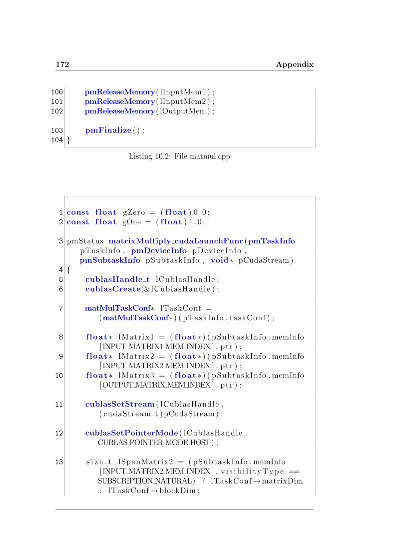
172 Appendix
100 pmReleaseMemory( lInputMem1 ) ;101 pmReleaseMemory( lInputMem2 ) ;102 pmReleaseMemory( lOutputMem) ;
103 pmFinalize ( ) ;104 }
Listing 10.2: File matmul.cpp
1 const f loat gZero = ( f loat ) 0 . 0 ;2 const f loat gOne = ( f loat ) 1 . 0 ;
3 pmStatus matrixMultiply cudaLaunchFunc (pmTaskInfopTaskInfo , pmDeviceInfo pDeviceInfo ,pmSubtaskInfo pSubtaskInfo , void∗ pCudaStream )
4 {5 cublasHandle t lCublasHandle ;6 cublasCreate(&lCublasHandle ) ;
7 matMulTaskConf∗ lTaskConf =(matMulTaskConf∗) ( pTaskInfo . taskConf ) ;
8 f loat ∗ lMatr ix1 = ( f loat ∗) ( pSubtaskInfo . memInfo[ INPUT MATRIX1 MEM INDEX ] . ptr ) ;
9 f loat ∗ lMatr ix2 = ( f loat ∗) ( pSubtaskInfo . memInfo[ INPUT MATRIX2 MEM INDEX ] . ptr ) ;
10 f loat ∗ lMatr ix3 = ( f loat ∗) ( pSubtaskInfo . memInfo[OUTPUT MATRIX MEM INDEX ] . ptr ) ;
11 cublasSetStream ( lCublasHandle ,( cudaStream t ) pCudaStream ) ;
12 cublasSetPointerMode ( lCublasHandle ,CUBLAS POINTER MODE HOST) ;
13 s i z e t lSpanMatrix2 = ( pSubtaskInfo . memInfo[ INPUT MATRIX2 MEM INDEX ] . v i s i b i l i t y T y p e ==SUBSCRIPTION NATURAL) ? lTaskConf→matrixDim: lTaskConf→blockDim ;

10.3 Matrix Multiplication Source Code 173
14 s i z e t lSpanMatrix3 = ( pSubtaskInfo . memInfo[OUTPUT MATRIX MEM INDEX ] . v i s i b i l i t y T y p e ==SUBSCRIPTION NATURAL) ? lTaskConf→matrixDim: lTaskConf→blockDim ;
15 cublasSgemm( lCublasHandle , CUBLAS OP N,CUBLAS OP N, ( int ) l lTaskConf→blockDim ,( int ) lTaskConf→blockDim ,( int ) lTaskConf→matrixDim , &gOne , lMatrix2 ,( int ) lSpanMatrix2 , lMatrix1 ,( int ) lTaskConf→matrixDim , &gZero , lMatrix3 ,( int ) lSpanMatrix3 ) ;
16 cublasDestroy ( lCublasHandle ) ;
17 return pmSuccess ;18 }
Listing 10.3: File matmul.cu

174 Appendix

Unicorn Publications
[1] Tarun Beri, Sorav Bansal, and Subodh Kumar. The unicorn runtime:
Making distributed shared memory style programming efficient for hybrid
cpu-gpu clusters. IEEE Transactions on Parallel and Distributed Systems,
2016 (Under Review).
[2] T. Beri, S. Bansal, and S. Kumar. A scheduling and runtime frame-
work for a cluster of heterogeneous machines with multiple accelerators.
In Parallel and Distributed Processing Symposium (IPDPS), 2015 IEEE
International, pages 146–155, May 2015.
[3] Tarun Beri, Sorav Bansal, and Subodh Kumar. Prosteal: A proactive
work stealer for bulk synchronous tasks distributed on a cluster of hetero-
geneous machines with multiple accelerators. In 2015 IEEE International
Parallel and Distributed Processing Symposium Workshop, IPDPS 2015,
Hyderabad, India, May 25-29, 2015, pages 17–26, 2015.
[4] Tarun Beri, Sorav Bansal, and Subodh Kumar. Locality Aware Work-
Stealing based Scheduling in Hybrid CPU-GPU Clusters. In Parallel and
Distributed Processing Techniques and Applications, 2015.

176 UNICORN PUBLICATIONS

Biography
Tarun Beri has passed his B.Tech. from Thapar Institute of Engineering
and Technology, Patiala and his M.S.(R) from Indian Institute of Technology
Delhi. His research interests include parallel and distributed systems, pro-
gramming languages and frameworks for heterogeneous environments, vector
graphics and machine learning. He holds several patents and publications in
his name.
The following is the list of papers published and communicated by Tarun
Beri:
1. Tarun Beri, Sorav Bansal, and Subodh Kumar. The Unicorn Run-
time: Making distributed shared memory style programming efficient
for hybrid CPU-GPU clusters. In IEEE Transactions on Parallel and
Distributed Systems, 2016 (Communicated)
2. Tarun Beri, Sorav Bansal, and Subodh Kumar. A scheduling and run-
time framework for a cluster of heterogeneous machines with multi-
ple accelerators. In Parallel and Distributed Processing Symposium,
IPDPS 2015, (Accepted)
3. Tarun Beri, Sorav Bansal, and Subodh Kumar. Prosteal: A proac-
tive work stealer for bulk synchronous tasks distributed on a cluster of
heterogeneous machines with multiple accelerators. In 2015 IEEE In-
ternational Parallel and Distributed Processing Symposium Workshop,
IPDPS 2015 (Accepted)
4. Tarun Beri, Sorav Bansal, and Subodh Kumar. Locality Aware Work-
Stealing based Scheduling in Hybrid CPU-GPU Clusters. In Parallel

178 Biography
and Distributed Processing Techniques and Applications, PDPTA 2015
(Accepted)
The following is the list of patents held by Tarun Beri:
1. US 8,316,337 - Method and System for Optimally Placing and Assign-
ing Interfaces in a Cross-fabric Design Environment (Issued Nov 20,
2012)
2. US 8,479,134 - Method and System for Specifying System Level Con-
straints in a Cross-fabric Design Environment (Issued July 2, 2013)
3. US 8,527,929 - Method and System for Optimally Connecting Interfaces
Across Multiple Fabrics (Issued Sep 3, 2013)
4. US 8,650,518 - Method and Apparatus for Rule based automatic Layout
Parasitic Extraction in a Multi-Technology Environment (Issued Feb
11, 2014)
5. Method and Apparatus for managing calendar entries in a document
(Filed Dec 19, 2013)
6. Method and Apparatus for controlling display of digital content using
eye movement (Filed Apr 28, 2014)
7. Fast, Coverage-Optimized, Resolution-Independent and Anti-aliased
Graphics Processing (Filed Mar 21, 2016)
8. Non-Multisampled Anti-aliasing for Clipping Paths (Filed May 23,
2016)
9. Dynamic Spread Anti-Aliasing (Filed Jul 27, 2016)


![Computational and Communication Complexity in Massively ... · Models of parallel computation •Bulk-Synchronous Parallel Model (BSP) [Valiant,90] Pro: Most general, generalizes](https://img.dokumen.tips/doc/110x75/60109df07ab6ef08e151e587/computational-and-communication-complexity-in-massively-models-of-parallel-computation.jpg)