Unfolding 3D Laser Images of

Underground Tunnels

Po Kong Lai, School of Electrical Engineering & Computer Science, University of Ottawa

Claire Samson, Dept. of Earth Sciences, Carleton University

AGU-CGU-GAC-MAC Joint Assembly

May 4th 2015

Montreal, Québec

Motivation & Goals

• Visualization of 3D mesh models of tunnels requires:

– Multiple vantage points

– Dedicated high-performance and costly hardware in field

• Main Goal:

– Take a triangulated mesh model generated from a point

cloud of an underground tunnel and convert it into a 2D

map

– The final 2D map should be easy and intuitive to interpret

1

Dataset

• Subsection of large underground tunnel

Outside View – Double Sided Lighting

41 m

8.2 m

6.7 m

2

3

Background Theory

• Well studied problem in differential geometry

– Known as surface parametrization

• Very few surfaces can be mapped from 3D to 2D

without error

– Error is known as metric distortion

– Visualized as stretching and shearing of the surface

– The degree of stretching and shearing described through

the Jacobian matrix

4

Surface Parameterization

• Given:

– Surface 𝑆 ∈ ℝ3

– Parameter domain Ω ∈ ℝ2

• Find a bijective function 𝑓 such that:

– 𝑓 ∶ 𝑆 → Ω

– 𝑓−1 ∶ Ω → S

• When 𝑆 is a mesh, the problem is known as mesh

parameterization

5

Mesh Parameterization

• Let 𝑀 be a mesh with the following parametric

representation:

• The partial derivatives 𝑓𝑢 and 𝑓𝑣 are vectors which

maps movement in Ω to 𝑀

𝑓 𝑢, 𝑣 = (𝑥 𝑢, 𝑣 , 𝑦 𝑢, 𝑣 , 𝑧 𝑢, 𝑣 ), where 𝑢, 𝑣 ∈ Ω

6

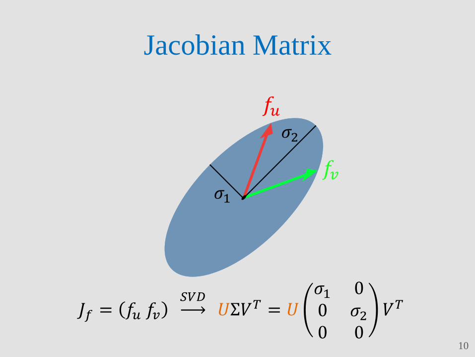
Jacobian Matrix

𝐽𝑓 = 𝑓𝑢 𝑓𝑣 𝑆𝑉𝐷

𝑈Σ𝑉𝑇 = 𝑈𝜎1 00 𝜎20 0

𝑉𝑇

𝑓𝑢

𝑓𝑣

7

Jacobian Matrix

𝑓𝑢

𝑓𝑣

8

𝐽𝑓 = 𝑓𝑢 𝑓𝑣 𝑆𝑉𝐷

𝑈Σ𝑉𝑇 = 𝑈𝜎1 00 𝜎20 0

𝑉𝑇

Jacobian Matrix

𝜎1 𝜎2

𝑓𝑢

𝑓𝑣

9

𝐽𝑓 = 𝑓𝑢 𝑓𝑣 𝑆𝑉𝐷

𝑈Σ𝑉𝑇 = 𝑈𝜎1 00 𝜎20 0

𝑉𝑇

Jacobian Matrix

𝜎1

𝜎2

𝑓𝑣

𝑓𝑢

10

𝐽𝑓 = 𝑓𝑢 𝑓𝑣 𝑆𝑉𝐷

𝑈Σ𝑉𝑇 = 𝑈𝜎1 00 𝜎20 0

𝑉𝑇

Jacobian Matrix

𝑁 Tangent Plane

3D Surface

𝜎2

𝜎1

𝑓𝑢

𝑓𝑣

11

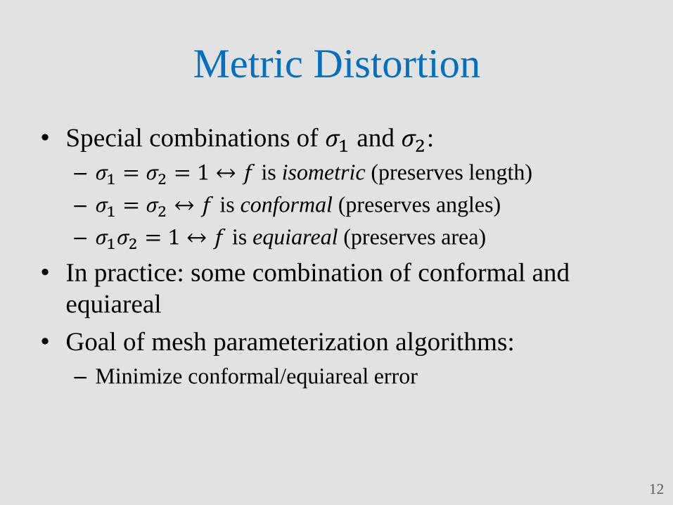
Metric Distortion

• Special combinations of 𝜎1 and 𝜎2:

– 𝜎1 = 𝜎2 = 1 ↔ 𝑓 is isometric (preserves length)

– 𝜎1 = 𝜎2 ↔ 𝑓 is conformal (preserves angles)

– 𝜎1𝜎2 = 1 ↔ 𝑓 is equiareal (preserves area)

• In practice: some combination of conformal and

equiareal

• Goal of mesh parameterization algorithms:

– Minimize conformal/equiareal error

12

Mesh Parameterization Methods

• Examined two state-of-the-art methods:

– Least Squares Conformal Mapping (LSCM)

– Angle Based Flattening (ABF++)

• LSCM

– Minimize conformal error per triangle: 𝐸𝑡 = 𝜎1,𝑡 − 𝜎2,𝑡2

• ABF++

– Minimize difference between 3D angles and 2D angles of

the triangles

13

Strike & Dip Visualized on Mesh

14

LSCM and ABF++ Results

LSCM ABF++ 15

Why the strange shape?

• Both methods are optimization based and thus has no

constraint for intuitive interpretation

• Any “bumps” are flattened

• To preserve the 3D surface area it must be displaced

in the 2D map

• Large number of bumps results in unintuitive final

shape

16

Mesh Deformation and Projection

Strategy

• Apply a global function, 𝐺 𝑣, 𝑑 to all vertices

– Implemented in Blender as a modifier

– Rotates the outer vertices at a greater rate than the inner

vertices

• Manually determine 𝑑 and position mesh to be

projected onto a 2D plane

17

Example

18

Example

19

Example

20

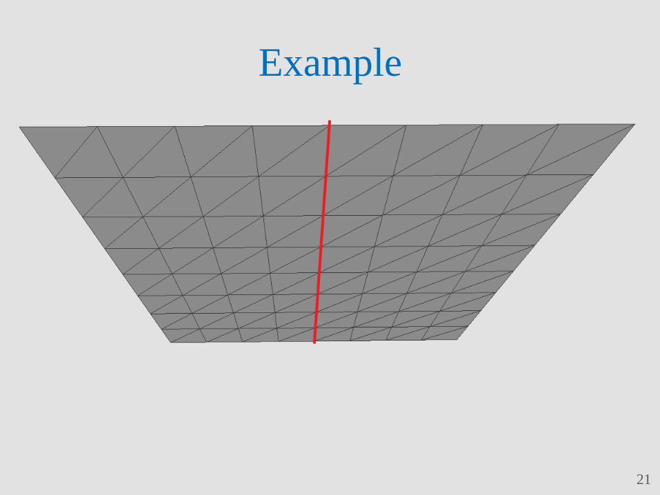
Example

21

v

u

(0,0)

Tunnel Mesh Deformed

22

Strike & Dip Visualized on Mesh

23

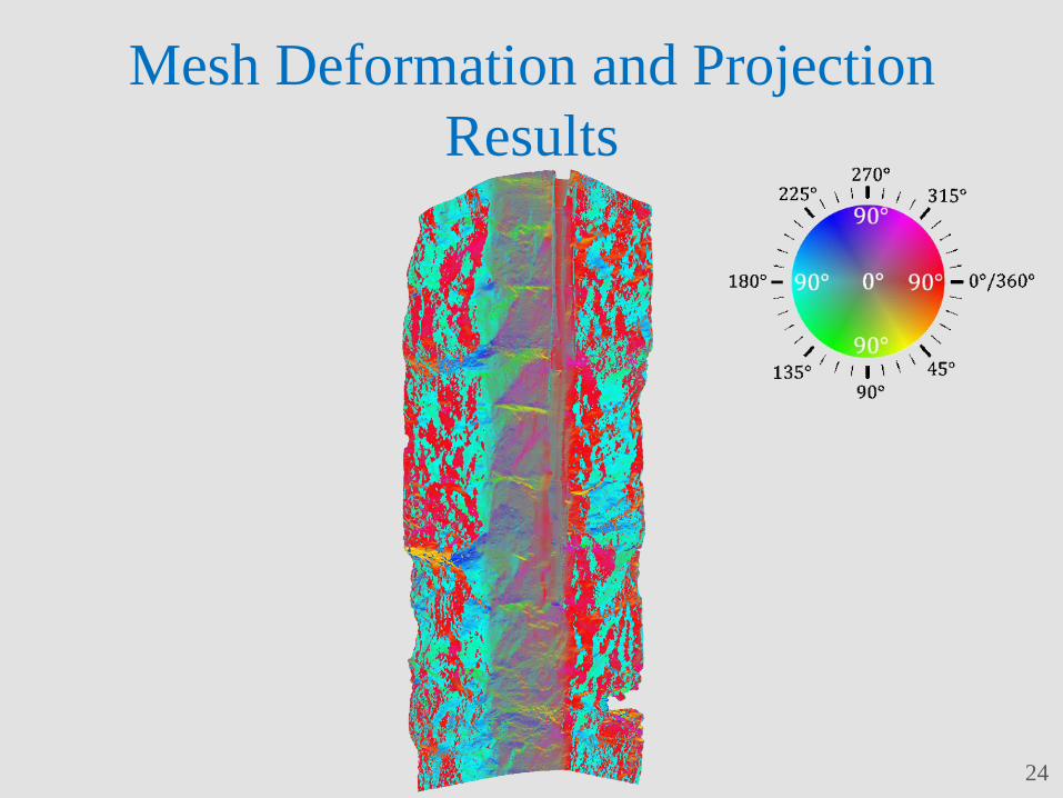
Mesh Deformation and Projection

Results

24

Metric Distortion Evaluation

• Utilize measures found in differential geometry

• Stretch 𝐿2

– 𝐿2 𝑡 =𝜎1,𝑡2 +𝜎2,𝑡

2

2 where t is a triangle in mesh 𝑀

– 𝐿2 𝑀 = 𝐿2 𝑡

2𝐴𝑟𝑒𝑎 𝑡𝑡∈𝑀

𝐴𝑟𝑒𝑎 𝑡𝑡∈𝑀

• Angular distortion

– 𝐴𝑛𝑔𝐷 𝑀 = 𝜃3𝑑−𝜃2𝑑

2𝜃3𝑑,𝜃2𝑑 ∈𝐴

𝐴 where 𝐴 is the set of

angle pairs

25

Metric Distortion Evaluation

Unfolding Method Stretch 𝐿2 Angular Distortion

LSCM 636554 0.0404

ABF++ 357237 0.0390

Mesh Deformation

& Projection

228 0.0814

26

Metric Distortion Visualization

ABF++ Mesh Deformation

&

Projection 27

Summary

• Mesh parameterization algorithms:

– Automatic

– Introduces the least amount of angular distortion

– Produce unintuitive 2D maps

• Mesh deformation and projection strategy

– Requires user input

– Good compromise between angular and stretch distortion

– Produces intuitive 2D maps

28

Conclusion

• Best approach for unwrapping 3D mesh models of

tunnels:

– First apply automatic mesh parameterization

– Perform mesh deformation and projection if

parameterization is not satisfactory

29

References

1. Hormann, Kai, Bruno Lévy, and Alla Sheffer. “Mesh parameterization:

Theory and practice.” (2007).

2. Lévy, Bruno, et al. “Least squares conformal maps for automatic texture

atlas generation.” ACM Transactions on Graphics (TOG). Vol. 21. No. 3.

ACM, 2002.

3. Sheffer, Alla, et al. “ABF++: fast and robust angle based

flattening.” ACM Transactions on Graphics (TOG) 24.2 (2005): 311-330.

4. Blender. http://www.blender.org/foundation/

5. MeshLab. http://meshlab.sourceforge.net/

6. ALICE Graphite. http://alice.loria.fr/WIKI/index.php/Graphite/Graphite

30