Unevenly distributed benefits of international

migration: evidence from Bangladesh.

Silvio Traverso

University of Florence, Dept. of Economics and Management

silvio.traverso@unifi.it

Within the framework of Rubin's causal model, this paper estimates the effects ofinternational migration on the welfare of Bangladeshi migrant households. Moving from the

estimation of the average effect, the paper disaggregates the impact on the basis ofhouseholds' quartile of expenditure and length of the migration period. The no-migration

counterfactual scenario is then used to measure the effect on inequality and to build atransition matrix showing the relationship between migration/remittances and social

mobility. The paper argues that those who benefit most from migration are the relativelybetter off households and that migration and remittances are both a source of inequality and

a vehicle of social mobility. Finally, since most of the characteristics which seem todetermine the probability of migration cannot be affected by governmental policies, it is also

argued that the resources deployed for pro-migration policies cannot directly benefit thepoorer sections of the population.

Keywords: International migration; Social mobility; Inequality; Counterfactual framework; Matchingestimators; Bangladesh.

JEL classification: F22; D63; O12; O15; O53.

Acknowledgments. I am indebted to Mariapia Mendola for her kind help and insightfuladvices. I would also to thank Simone Bertoli for his comments in the preliminary stages of

the research and Gianna Claudia Giannelli for having read a final draft of the paper. Thatsaid, any remaining mistakes are on my own.

1

1. Introduction

Since the beginning of the nineties, Bangladesh recorded significant progress in terms of all main

social and economic indicators. The growth of real incomes, along with remarkable improvements

in health and food security, induced some scholars to talk about a “Bangladesh surprise” (Asadullah

et al., 2014). During this period, the country experienced a profound change and the emergence of

international migration can be considered one of the distinguishing features of such transformation.

Indeed, over the 2000-2010 period, Bangladesh was the country that registered the highest average

number of net emigrants per year (UN, 2013). The surge in migrants' remittances mirrored the

increase in the stock of international migrants. Officially recorded remittances outweighed official

development assistance in the mid-nineties (Mohapatra et al., 2010) and in 2013 they were worth

more than 10% of national GDP. In the recent history of Bangladesh, international migration and

economic development appear deeply interconnected. Low domestic wages, overpopulation and

environmental vulnerability worked jointly as push factors for outward migration, which has

become an increasingly common “livelihood strategy” for households and individuals (Siddiqui,

2003). On the other hand, even though migration is a result of the limited economic opportunities

available domestically, it can also be regarded as a key factor for recent social and economic

development of the country (Bangladesh Bank, 2013; Siddique et al., 2012). Surprisingly, despite

the general recognition of the potential contribution of migrants' remittances to the welfare of

Bangladeshi households and despite the importance of Bangladesh itself as a “test case for

development” (Faaland and Parkinson, 1976), the literature on migration and remittances has not

yet produced a specific country-study. The contribution of this paper is twofold: on the one hand, it

represents the first attempt to estimate the impact of migration and remittances in Bangladesh on the

basis of a national representative survey; on the other, taking full advantage of the non-parametric

nature of matching estimators, it studies the phenomenon from multiple perspectives. Specifically,

the impact of migration is disaggregated by quartile of expenditure and households' counterfactual

outcomes are used to build a transition matrix showing the effect of migration on migrant

households' position in the expenditure distribution and to compute Bangladesh's Gini index in a

no-migration counterfactual scenario. The paper finds that the relative magnitude of the positive

effect is higher for the households belonging to lower expenditure quartiles and becomes negative

(but not statistically significant) for the richest migrant households. Migration turns out to be

successful in approximately half of the cases and it can be considered an important vehicle of social

mobility. It also emerges that most of the international migrants come from relatively better-off

households and that migration and remittances contributes to a modest increase in inequality.

Finally, it comes out that the impact of migration tends to grow over time, supporting the idea that

2

part of remittances are directly used for productive investment. Sensitivity checks prove that the

results are robust to the introduction of different equivalence scales, even if the technical choices

regarding households' economies of scale may considerably affect the magnitude of the impact.

With regard to policy considerations, the analysis shows that most of the factors which influence the

probability of migration seem to be beyond the scope of any policy intervention, meaning that the

resources allocated in pro-migration policies cannot directly benefit the poorest households. The

rest of the paper is organized as follows. Section 2 explores the literature, sections 3 and 4 describe

data and methodology, section 5 illustrates the empirical strategy, section 6 discusses the results and

some policy implications, section 7 concludes.

2. Literature review

The economic literature on migration and remittances is vast and the multidimensional nature of the

subject favoured the emergence of several specific strands. The unit of analysis allows to make a

first broad distinction between microeconomic and macroeconomic works. Macroeconomic studies

relate the aggregate flows of migrants and remittances to other aggregate variables such as

exchange rates (Lartey et al., 2012) and GDP growth rates (Kumar and Stauvermann, 2014),

microeconomic works focus either on households or individuals. Secondly, some works focus on

the countries of origin and others on the countries of destination. Thirdly, whereas some studies

evaluate the relation between migration and socio-economic variables, others investigate the

determinants of migration and remittances choices (Agarwal and Horowitz, 2002; Stark and Lucas,

1988) or explain who migrants are and in what they differ from stayers (Borjas, 1987). Finally, even

though migration and remittances can be conceived as the two faces of a same coin, they are often

treated separately: part of the literature focuses on migration, another part concentrates on

remittances and some works emphasise the simultaneity of the two phenomena. As pointed out by

Hanson (2010), because of such great abundance of perspectives, economic literature has still not

been able to build a “Washington consensus” on migration and remittances. In particular, whereas

literature on remittances tends to highlight their positive developmental impact, migration literature

has paid more attention on the potential adverse effects of the phenomenon.

According to Ratha (2006), workers' remittances constitute the most tangible link between

migration and the development of receiving countries, producing micro and macro direct positive

effects. Indeed, the empirical evidence produced by several country-case (Bertoli and Marchetta,

2014; Combes et al., 2014; Jimenez-Soto and Brown, 2012; Lokshin et al., 2010) and cross-country

(Acosta et al., 2008; Gupta et al., 2008; Adams and Page, 2005) studies suggests that remittances

play an effective role in reducing poverty. Besides the direct wealth effect on recipient households,

3

Adams and Cuecuecha (2013, 2010) found that recipient households exhibit a higher marginal

propensity to spend in investment goods and Giuliano and Luiz-Arranz (2009) demonstrated that

remittances flows constitute an alternative source of investment financing, especially in countries

characterized by a low level of financial development. Moreover, because of their substantial

volume and moderate volatility, remittances constitute a safe source of foreign-exchange earnings,

increasing recipient countries' creditworthiness and improving their capacity to cope with capital

flights (WB, 2006). As anticipated, notwithstanding the mixed findings regarding inequality

(Acosta et al., 2008; Brown and Soto, 2008; Barham and Boucher, 1998) and exchange rates

(Lartey et al., 2012; Amuedo-Dorantes and Pozo, 2004), literature focussing on remittances seems

to have reached a certain degree of consensus regarding their beneficial effects. On the contrary,

since the literature on migration produced somewhat mixed results, scholars tend to be cautious in

associating migration and development and have identified a number of migration's negative effects

on sending countries' economic performances. Even though Mishra (2007), studying Mexican

emigration over a thirty-years period, estimated a major redistributive effect from capital to labor

remuneration at the cost of a small negative effect on GDP, “brain drain” literature pointed out how

migration might actually cause a significant depletion of human capital (Wong and Yip, 1999;

Beine et al., 2001). Taking advantage of a natural experiment, Gibson et al. (2011) found a negative

effect of migration on several migrant households' indicators and other empirical studies produced

similar results for what concerns children's education (McKenzie and Rapoport, 2011; Giannelli and

Mangiavacchi, 2010) and on mental problems of left-behind household members (Graham et al.,

2015).

For what concerns to the specific case of Bangladesh, Siddique et al. (2012) found a one-way

positive causal relationship from remittances to GDP growth while Chowdhury (2011)

demonstrated the existence of a similar relationship between remittances flows and financial

deepening. Such results are somehow consistent with the conclusions of Stahl and Habib (1989),

who argued that even though remittances are used by recipient households just for consumption

expenditure, they nevertheless can indirectly trigger investment through their boosting effect on

aggregate demand. As far the socio-economic implications of migration, Mendola (2008) found that

household involved in international migration were more prone to invest in modern agricultural

technology and Hadi (2001) argued that it can be interpreted as a determinant of behavioural change

in the traditional rural communities of sending areas, prompting a relaxation of women's socially

approved habits.

4

3. Data

This study employs the data collected during the 15th round of Bangladesh Household Income and

Expenditure Survey (HIES), held between February 2010 and January 2011. HIES is a national

representative survey conducted by the Bangladesh Bureau of Statistics in collaboration with the

World Bank and, containing a wide and deep range of socio-economic information both at the

individual and household level, is considered the most accurate and comprehensive source of data

for what concerns the social and economic accounts of Bangladesh households. In particular, HIES

2010 collects data on 12,240 households, for a total of 55,580 individuals. The questionnaire

includes sections on expenditure, income, consumption, education, employment, health, households'

assets and – among others – migration. The module on migration gathers a relatively large set of

information on 1,372 international and 728 domestic migrants who, before migrating, were part of

the surveyed households. On the basis of this information, (international) migrant households are

defined as those households satisfying at least one of the two following conditions: (i) the

household has reported to currently have one (or more) member migrated abroad; (ii) one (or more)

member of the household is reported to have been abroad for more than six consecutive months

during the previous five years. Since the aim of the analysis is to evaluate the impact of migration

on the welfare of migrant households, condition (ii) prevents to discard from the pool of migrant

households those families whose welfare is likely to be still affected by the migration experience of

their recent past. Following this definition, it results that 10.4% of Bangladeshi households can be

considered as “migrant households”. It also turns out that, among households satisfying condition

(i), the average number of migrants is 1.18 and almost all of them (98.4%) are male. In general, the

share of migrant households which received remittances in the previous twelve months is 82.0%,

but it raises to 91.7% considering only the subgroup of migrant households which satisfy condition

(i). It should also be noted that, adopting households (rather than individuals) as unit of analysis, the

present work implicitly adheres the framework on the new economics of labor migration (NELM).

This framework, pioneered by Stark (Stark and Levhari, 1982; Stark and Lucas, 1988) in relation to

rural-urban migration, models migration as the outcome of a dynamic contract between migrants

and their families, implying that migration decisions are collectively taken at the household level.

5

4. Methodology

4.1. Measuring welfare

This research considers the wellbeing of individuals in terms of their command over goods and

services, conceived as the inputs of individual utility. Consumption (proxied by per capita

expenditure) allows to convey it into a monodimensional money-metric measure which, compared

to income, is less subject to measurement error and characterised by a lower volatility. It is worth

noting that, because of consumption smoothing, expenditure should (at least partially) discount for

the lumpy costs of financing migration. On a theoretical level, per capita consumption is formalised

as

Yi = e(p, ui ) / d(xi )

where e(.) is the household expenditure function, d(.) the equivalence scale function, p a n-

dimensional vector containing the prices of all the goods and services available in the market, x a k-

dimensional vector of relevant household characteristics and u the (maximised) level of utility of

the household. Total expenditure is defined by function e, which is nondecreasing, continuous,

concave, homogeneous of degree 1 in p. The equivalence scale function d is meant to standardises

household size on the basis household characteristics, allowing to compare the welfare of

individuals belonging to households which differ in size and demographic composition. In practice,

per capita consumption is estimated from the consumption section of the household survey. Since

6

Table 1. Households' descriptive statisticsOverall Non migrant Migrant Matched

Household size 4.65 4.51 5.89 5.96Kids (aged 6-17) 1.29 1.28 1.40 1.39Male adults (aged 18-45) 0.98 0.91 1.58 1.63Male adults (aged 46-65) 0.34 0.33 0.42 0.42Female adults (aged 18-45) 1.02 1.00 1.19 1.17Female adults (aged 46-65) 0.30 0.29 0.44 0.46Adults, old (aged 66+) 0.19 0.18 0.25 0.26Years of education, adult males 4.36 4.37 4.28 4.66Years of education, adult females 3.63 3.52 4.50 4.55Urban (municipality) 26.80% 27.02% 24.94% 24.48%Urban (metropolitan area) 9.15% 9.48% 6.35% 7.23%Muslim 87.79% 86.94% 94.97% 95.22%Landless 6.38% 6.85% 2.40% 2.35%Semi-landless (<0.05 acres) 23.25% 24.60% 11.85% 11.83%

N 12,240 10,949 1,291 3,873Source: Author's calculations, HIES 2010.

HIES does not provide sufficient information to implement a rental equivalent approach, following

Deaton and Zaidi (2002), the consumption flow of durable goods is estimated assuming an annual

depreciation rate of 10%. For what concerns the equivalence scale functions, the most elementary

one simply returns the number of household members whereas others, less trivial, use more of the

information of x (i.e. the age of members). The scales adopted in the paper are described in OECD

(2013).

4.2. Counterfactual framework and treatment effect

The impact of migration and remittances on household welfare can be evaluated by comparing the

measures of the reference indicators actually observed with those which would have been witnessed

in a no-migration counterfactual scenario. The key assumption behind all the analyses conducted in

a counterfactual framework is that every analytical unit belonging to the population of interest has a

potential outcome under each treatment state (Morgan and Winship, 2007). Adopting this

framework, the impact of the exposure to a treatment (with respect to the exposure to an alternative

set of causes) on a given analytical unit is the difference between the outcomes associated to the two

treatment states. Since it is possible to observe (at most) only one outcome for each unit, causal

inference can be conceived as a problem of missing data (Imbens and Rubin, 2015; Holland, 1986).

In the case of a binary treatment, the observational rule for the outcome of the variable of interest Y

can be formalised as:

Yiobs = Di Yi

(1) + (1 – Di) Yi(0)

where Yi(0) and Yi

(1) indicate the two potential outcomes of the variable of interest of the i-th

observation and Di is a binary variable indicating the exposure to one of the two alternative sets of

causes, treatment (Di=1) and control (Di=0). In the present analysis, the variable of interest is the

logarithm of per capita expenditure (computed on a household-level basis) and the treatment is

defined as currently having, or having had in the previous five years, at least one member emigrated

abroad. It follows that treated and migrant households coincide. As the observational rule imposes,

for every individual it is possible to observe either Yi(0) or Yi

(1), depending on whether the i-th

household has been exposed to the treatment and the individual treatment effect is defined as:

τi = Yi(1) – Yi

(0) .

Since the research aims to evaluate the impact of migration on each migrant household, the

7

fundamental quantity of interest is

τitreat = (Yi

(1) – Yi(0) | Di = 1)

and it is obtained by estimating the unobserved potential outcomes (Yi(0)) of migrant households (the

estimator for individual effects is described in section 5.12). The expected value of τitreat is the

average treatment effect on the treated (ATET) that, defined as

ATET = E ( Yi(1) – Yi

(0) | Di = 1 ) ,

represents the average impact of migration and remittances on the welfare of the migrant

households members expressed in percentage change of their expenditure. In order to estimate the

effect of migration on households belonging to different quartiles of expenditure or characterized by

a different length of exposure to the treatment, the expected value of the treatment effect is

conditioned not only by the exposure to the treatment, but also on the set of condition Θi . The

estimator is thus defined as

ATET|Θ = E ( Yi(1) – Yi

(0) | Di = 1, Θi )

where Θ contains the set of additional conditions, e.g. the quartile of expenditure of the household

in the counterfactual scenario.

4.3. Methodological issues

As pointed out by migration literature, the estimation of the impact of migration and remittances on

the welfare of those left behind raises a series of methodological issues. Following the classification

provided by Adams (2012), these issues can be summarised as those arising because of (a) the

simultaneity of the decisions regarding migration with other choices (labor supply, education,

fertility, etc.) that also influence the outcome of the variable of interest, (b) the self-selection of

migrants, who systematically differ from the stayers, (c) the reverse causality nexus between

poverty and migration/remittances and (d) the presence of relevant omitted/unobservable variables.

On a theoretical level, a randomised experiment would allow to overcome all these difficulties and

to estimate an unbiased average treatment effect (ATE = E (Yi(1) – Yi

(0)) ), but the nature of migration

phenomenon makes this solution infeasible. Natural experiments, allowing to fully overcome the

problem of self-selection and to estimate an unbiased ATET, can be considered as the first-best

8

feasible methodological solution. Unfortunately they are rare and the few, as in the case of the New

Zealand's visa lotteries, have been heavily exploited (Gibson et al., 2013, 2011, 2010; Stillman et

al., 2009). Moreover, even though these studies adhere to the best methodological practice, they

often do not allow to focus on very representative case-studies. In the absence of available natural

experiments, regression-based approaches result to be the most common methodological solution

and the variable of interest is expressed as a linear function of a set of exogenous explanatory

variables. Regression-based approaches relate causality with the notion of ceteris paribus

(Wooldridge, 2010) and, usually, the treatment effect is the estimated coefficient of a treatment

indicator. In order to address the above-mentioned methodological issues, it is usually implemented

the Heckman's correction procedure (Heckman, 1979) or, alternatively, scholars resort to

instrumental variables (IV) estimator. In practice, since the relevance of the instruments can only be

tested from a statistical point of view and their exogeneity can not be tested at all, finding

appropriate instrumental variables turns out to be everything but easy (Jalan and Ravallion, 2003).

On the other hand, as pointed out by Puhani (2000), the results obtained using a Heckman's two-

stage model may be misleading if normality assumption is violated.

4.4. Matching methods

In social sciences, matching methods gained momentum after the works of Dehejia and Wahba

(1999, 2002) and found application in a number of migration studies (Bertoli and Marchetta, 2014;

Möllers and Meyer, 2014; Jimenez-Soto and Brown, 2012; Ham et al., 2011). Whereas these works

rely on propensity scores, the present study perform matching on linearised propensity scores (see

section 5.11), which produce better matches and a more precise identification of the overlapping

region. The main theoretical difference between regression-based and matching methods lies in the

notion of causality implicitly arising from a different interpretation of the covariates. Indeed,

according to Imbens and Rubin (2015), regression models only rely on observed outcomes and fail

in drawing an explicit distinction between potentially causal treatments and intrinsic attributes of

the units under examination. They also argue that the ATET of the two approaches coincide only in

the special case of a linear regression without additional covariates in the context of a completely

randomised experiment. On a practical level, matching methods present three main advantages.

Firstly, because of their non-parametric nature, the estimates of the counterfactual outcomes do not

directly rely on the specification of any particular functional model. Secondly, the estimated

treatment effect is not constant but different for every unit. Thirdly, the balance of the covariates

ensures that matched observations really resemble the treated ones.

Conditional independence is the fundamental assumption behind matching and requires that, after

9

controlling for an appropriate set of exogenous covariates X, potential outcomes are orthogonal to

treatment assignment (households' migration status). Formally:

(Yi(0), Yi

(1)) ╨ Di | Xi

Conditional independence is a necessary but not sufficient condition to implement matching

methods in observational studies, which additionally require the observable nature of the set of

covariates X (selection on observables assumption). Under selection on observables, it is possible to

estimate the treatment effect matching treated units with untreated ones which exhibit the same

value of X. Since Xi is a k-dimensional vector, the probability of finding a match between treated

and untreated units exponentially decrease with the increasing of k (and falls to zero in presence of

continuous covariates). This difficulty, known as “curse of dimensionality”, has been addressed by

Rosenbaum and Rubin (1983), who defined a function f : Rj → { R ∩ (0, 1) } such that

f(Xi ) = Prob[Di = 1 | Xi ]

and demonstrated that

(Yi(0), Yi

(1)) ╨ Di | f(Xi )

where f(Xi) acts as a balancing score and, when represents the unit-level probability of selection into

the treatment, it is called propensity score. Propensity scores can be estimated with a probability

model and allow to match households on the basis of a monodimensional measure, overcoming the

dimensionality problem. Each migrant household is matched with one or more households which

share the same characteristics except for the exposure to the treatment and the outcomes of matched

untreated households are used to estimate the unobservable potential outcomes of migrant ones. The

validity of the (weak) overlapping condition, given by

Prob[Di = 1 | f(Xi) ] < 1 Ɐ i ,

ensures that it is possible to estimate the ATET for the entire subsample of treated units.

It is worth stressing that, if selection on observables holds (which is equivalent to say that issue (d)

is not a cause of concern), matching methods provide a solution for issues (a) and (b). Indeed, they

allow to correct for the self-selection of migrant households and the estimates take into account the

10

effect that remittances and changes in household's composition may have on the opportunity costs

faced by household members (which can affect, inter alia, individual labor supply). Even though

selection on observables cannot be tested, this concerns is mitigated by the fact that HIES 2010

presents a large sample size, a favourable treated-untreated ratio and, covering a wide range of

topics, allows to estimate the balancing scores on an uncommonly large set of information.

4.5. Caveats

Firstly, it should be noted that considering only two potential outcomes for each unit implicitly

introduces the stable unit treatment assumption (SUTVA). In economic terms, it means that the

estimates only account for partial equilibrium effects and do not consider the effects that migration

and remittances may produce, for example, on aggregate demand, exchange rate, wages and

unemployment. Consequently, the estimates can be considered robust for the marginal migrant

household but the counterfactual scenario should rather be considered as a nuanced benchmark.

Secondly, the survey does not provide information regarding the endogenous recomposition which

some migrant households could experience. For instance, this phenomenon may take place when

the head of a household composed by three people (head/husband, wife and a child) emigrates and

the two left-behind members, looking for a more efficient household dimension, find convenient to

join the wife's brother family. When this newly-formed household is surveyed, it is recorded as a

migrant household and the migrant is registered as the brother-in-law of the head. Even in presence

of longitudinal data or of specific questions regarding the dynamics of household recomposition,

this situation would be challenging to handle. Indeed, the bifurcation introduced by the causal

exposure does not regard the outcomes of the households but the population of households itself.

On a theoretical level, finding a definition of the treatment would be extremely difficult and, on a

practical level, it would require an excessive amount of information. To misquote Eraclitus, it is not

possible to step twice in the same river, but sometimes it could be convenient to assume so.

5. Empirical strategy

This section illustrates the empirical strategy follwed in the study, explaining the main steps made

to obtain the final results, from the inclusion of the covariates to the choice of the estimator and the

check of overlapping and balance conditions.

5.1. Choice of the probability model and general rules for the inclusion of covariates

Estimation of propensity scores requires the choice of a probability model and the selection of the

11

identifying variables. A binary treatment calls for a binary response model and literature

recommends the use of either a probit or a logit model (Caliendo and Kopeinig, 2008). The paper

opted for a probit model. The probability of selection into the treatment is thus given by

Prob[Di=1 | X i] = f (X i) = Φ( X i ' β )

where Φ(.) is the c.d.f. of a standard normal distribution. The choice of the set of covariates X that

identifies the probability model is a crucial step because, in theory, they are the observable

conditioning variables which ensure the independence between potential outcomes and selection

into the treatment. In practice, being conditional independence an abstract concept, the covariates of

observational studies should not be conceived as the real conditioning variables but rather as

proxies capturing the maximum amount of households' relevant conditioning information. For this

reason, and because of the lack of direct interpretation of probit coefficients, as long as it improves

the quality of the estimates, there is no need to avoid the inclusion of interaction terms or nonlinear

transformations of the covariates (Imbens and Rubin, 2015). On the other hand, flexibility does not

mean theoretical inconsistency and the inclusion of every covariate needs to be theoretically

justified on the basis of the criteria of relevance and exogeneity. Included predictors should be

relevant in the sense that they simultaneously influence both the probability of the selection into the

treatment and the outcome of the variable of interest. On the other hand, exogeneity is meant as the

absence of any causal relationship moving from the exposure to the treatment to the predictors of

the probability model. Since the concept of causality is intrinsically related to time (Holland, 1986),

covariates whose value is already determined before the exposure to the treatment can generally be

considered as exogenous. It is worth noting that the final set of covariates used in this study

considerably differs from those adopted in other works which adopted similar methods: these

differences arise both because of theoretical considerations and of the structure of the dataset, which

makes available an uncommon amount of information. Finally, it has to be specified that the sets of

covariates on which propensity scores have been estimated do take into account the effect of

migration on household composition. In other words, before running the probability mode,

“missing” migrants members have been reintroduced in their original households.

5.2. Sample weights

As observed by Zanutto (2006), the use of sample weights should be avoided in the estimation of

probability model. Indeed, matching methods are strictly based on individual characteristics and,

consequently, all the information needed for the estimation of each score is entirely contained in the

12

correspondent unit. On the other hand, following DuGoff et al. (2014), sample weights have been

included among the predictors of propensity scores. This choice is justified by the fact that sample

weights, for their very nature, contain relevant information on the observation. Finally, the weights

has been used to generalise sample results to the entire population.

5.3. Demographic characteristics

Adopting a NELM theoretical framework, the demographic structure of the household is of a major

importance and should be adequately captured by X and the set of covariates describing household

demographic structure included in this study is wider and more detailed than the ones adopted by

similar works. Still, since migration affects post-treatment fertility choices, all the covariates

reflecting the demographic characteristics have been carefully computed in order to avoid this

source of endogeneity. Consequently, neither household dimension nor age dependency ratio, used

respectively by Jimenez-Soto ans Brown (2012) and Bertoli and Marchetta (2014), have been

included. By contrast, the predictors included in the model are the number of working age male and

female adult members (divided in two age groups, 18-45 and 46-65), the number of elderly

members and the number of kids between six and seventeen years old (under the hypothesis they

are old enough to be exogenous to migration).

5.4. Information on household head

The individual characteristics of household head are likely to be relevant in explaining both the

economic performance and the migration decision of the household and in some works they have

been included among the covariates (Möllers and Meyer, 2014; Jimenez-Soto and Brown, 2012;

Calero, 2009). Yet, as pointed out by Cox-Edwards and Oreggia (2009), in absence of adequate pre-

treatment information, household headship should be considered endogenous to migration and thus

excluded from predictors. Endogeneity of headship clearly emerges from Bangladesh data: the

percentage of female headed household is 13.9%, but it raises to 44.7% among migrant households

and falls to 10.3% in the non-migrant subsample. Such a remarkable difference can be explained by

the fact that, when the husbands emigrate, headship is inherited by wives.

5.5. Education

Economic theory recognizes a fundamental importance to human capital formation and the

educational attainment of household members is likely to be a key predictor for both household

consumption and migration propensity. In the case of Bangladesh, since the returns on education

and the average level of education differ between males and females, this information has been

13

disaggregated according to a sex-wise criterion. The level of education is thus captured by two

variables indicating the average years of education of female and male adult members, while the

educational attainment of younger members is excluded in order to avoid usual concerns about

endogeneity. HIES data on individual educational achievements have been converted into years of

schooling following the information on Bangladesh education system provided by UNESCO

(2011).

5.6. Households' environment

Besides the variables which capture information on households' demographic structure and human

capital endowment, literature has stressed the importance of households' local environment. These

information are captured by a set of regional dummies, by a dummy for households living in urban

areas and by another dummy for households living in one of the four metropolitan areas.

5.7. Religion

Since nine out of ten households are Muslim, since Islam is a pillar of national identity and since,

except for the “secularist” parenthesis of the rule of Mujibur Rahman, the country has historically

pursued policies inspired by a moderate islamism (Lewis, 2011), it is possible to conceive the

existence of a correlation between the average economic performance of the families and their

religious beliefs. On the other hand, since Muslim oil countries have traditionally been the

destination countries, household religion might also affect probability of migration. For these

reasons – and because its exogeneity – the religious belief of households has been included among

predictors.

5.8. Entrepreneurship

Entrepreneurial attitude of household members could be relevant in determining the economic

performance of the household they belong as well as the probability of migration. It can also be

considered as a proxy for other relevant unobservable characteristic. HIES 2010 has a section on

non-agricultural enterprise activities which contains information about the type of business the

household is involved in and when the activity started. This information allows to create dummies

for household's involvement in formal and informal non-agricultural business. In order to avoid

endogeneity issues, dummies activate only if the household started a business before the migration

of a member.

14

5.9. Other predictors

As discussed before, according to DuGoff et al. (2014), sample weights should be included among

the predictors. Other variables, as the access to public electricity network, might be used as

predictors, even though their exogeneity is less clear. The same goes for land ownership: on the one

hand, it surely affects both the well-being of household and the migration decision but, on the other

hand, it could be endogenous to migration (land could have been sold for financing migration or,

viceversa, could have been purchased with the remittances). Anyway, Bangladesh's land market is

characterized by a low volume of transactions (Mendola, 2008) and the dummies inserted into the

set of covariates only account for the two extremes of land ownership: landlessness/semi-

landlessness and, alternatively, the ownership of a large farm.

5.10. Specification of the probability model

The choice of the final specification of the probability model has been made following a stepwise

approach. Specifically, in the light of previous paragraphs' considerations, in each of the first six

15

Table 2. Specifications of the probability modelSpecifications A B C D E F G

Male adults (18-45) 0.000 0.000 0.000 0.000 0.000 0.000 0.000Male adults (46-65) 0.000 0.000 0.000 0.000 0.000 0.000 0.000Female adults (18-45) 0.193 0.014 0.015 0.013 0.015 0.101 0.003Female adults (46-65) 0.000 0.000 0.000 0.000 0.000 0.420 0.002Old adults (65+) 0.000 0.000 0.000 0.000 0.000 0.000 0.000Kids (6-17) 0.000 0.000 0.001 0.016 0.006 0.004 0.004

Education Male adults average education 0.000 0.000 0.000 0.000 0.000 0.000Female adults average education 0.000 0.000 0.000 0.000 0.000 0.000Regional dummies (χ²) 0.000 0.000 0.000 0.000 0.000Urban area 0.000 0.000 0.025 0.018 0.020Metropolitan area 0.000 0.000 0.000 0.000 0.000

Land ownership Landless 0.000 0.000 0.000 0.000Semi-landless (<.0.05 acres) 0.000 0.000 0.000 0.000Landlord (>4 acres) 0.469 0.750 0.588

Other variables Religious belief (Muslim) 0.000 0.000 0.000Entrepreneurship (formal) 0.000 0.000 0.000Entrepreneurship (informal) 0.000 0.000 0.000Access to electricity network 0.000 0.000 0.000Sample weights 0.000 0.000 0.000Squared male adults (18-65) 0.000 0.000Squared female adults (18-65) 0.253Male adults*Male education 0.000 0.000Female adults*Female education 0.283Squared male education 0.861Squared female education 0.001 0.000

McFadden's pseudo-R² 0.1109 0.1509 0.2103 0.2191 0.2747 0.2935 0.2932Log-likelihood -3667 -3502 -3257 -3221 -2991 -2914 -2915

Note: the table reports coefficients' p-values. Source: Author's calculations.

Demographic structure

Geographical variables

Interactions / Nonlinear transformations

steps it has been included an additional group of covariates. Table 2 reports coefficients' p-values,

the McFadden's pseudo-R2 and the log-likelihood of each specification (coefficient have no causal

interpretation and has been omitted). As expected, it emerges that almost all the variables discussed

in the previous paragraphs turn out to be significant in predicting the probability of selection into

the treatment, and every groups of variables significantly improves the statistical fit of the model.

The final choice has been on specification (G) and it is the one that will be used thereafter. On the

basis of the assumptions of the model and following Imbens and Rubin (2015), (G) mimics the unit-

level assignment probability function which, theoretically speaking, depends itself by the

assignment mechanism that rules the migration in Bangladesh.

5.11. Choice of the matching variable

The choice of the matching variable is a crucial step and can substantially affect final results.

Whereas most of the studies (Bertoli and Marchetta, 2014; Möllers and Meyer, 2014; Jimenez-Soto

and Brown, 2012; Mendola, 2007) match on the estimated propensity scores f ( X i) , in this

analysis matching is performed on the logit of the scores, defined as

ℓ ( X i)= log( f ( X i)

1 − f (X i))and conceivable as a linearised propensity score (lps). The main advantage of matching on this

monotonic transformation of propensity scores is due to the fact that it makes comparable the

distances between observations irrespectively of their position in the distribution, making the

matching procedure more precise. Moreover, on a practical level, it simplifies the identification of

the region of common support and ensures the theoretical consistency of the imposition of a caliper

(see below).

5.12. Matching estimator

The analysis makes use of a nearest neighbour matching (NNM) algorithm with replacement and

imposing a caliper. With NNM, the counterfactual outcome of each treated unit is estimated taking

the average of the closest M untreated observations (in the present analysis, M = 3). Formally,

building on Abadie et al. (2004), IM(i) is defined as the set of the indices for the matches of the i-th

unit that are at least as close as the M-th match (distance dM) and, in any case, not more distant than

dcaliper

I M (i) = {l=1,... , N | Dl=0 , abs [ ℓ ( X i)− ℓ(X l)]⩽min [d M (i) , d caliper ]}

16

and the estimator for Yi(0) results

Y i

(0) =1

# I M (i) ∑l∈ IM (i )

Y l

where # IM(i) is the number of the matches of the i-th unit. As pointed out by Smith and Todd

(2005), the increase of M reduces the variance of the estimator (it uses more information) at the

expenses of the bias (incremented, since the average quality of the matches will be lower). For what

concerns replacement, as in the case of Dehejia and Wahba (2002), it results necessary because, for

high values of the logit, there is a relative abundance of treated observations.

5.13. Common support

The estimation of all the counterfactual outcomes requires that every treated unit is matched with at

least one unit exposed to the control treatment. This condition is satisfied when the region of

common support, the overlapping region between the p.d.f. of the logit for treated and untreated

units, coincide with the region in which the p.d.f. of the logit of treated units assumes positive

values. The imposition on a caliper, a maximum distance between two logit in order to be

considered “close enough” for matching, offers a straightforward solution to the common support

problem. According to Austin (2011), when at least one of the predictors is not binary, the optimal

caliper width should range between 0.2 and 0.55 the standard deviation of the estimated logit.

Choosing specification (G) and imposing a caliper of 0.5 times the standard deviation of lps, the

caliper width (dcaliper) turns out to be 1.159, large enough to match all the treated units.

5.14. Balance

From a certain perspective, matching can be seen as a method of strategic subsampling (Morgan

and Winship, 2007) based on the observables relevant covariates contained in X and aimed to pick

up, among untreated units, a counterfactual group which shares the same characteristics of the

treated one. In the present case, balance is achieved if the condition

Di ╨ Xi | ℓ (Xi)

is verified. When the estimand is the treatment effect on the treated, the subsampling is among the

untreated observations. Hence, the quality of the estimates crucially depends on the balance of the

17

conditioning covariates among the treated and matched control groups. Getting a look at the

distribution of the lps before and after the matching can provide a first insight of balance

achievement [Appendix, fig. A1]. Secondly, following Sianesi (2004), the regression of the

probability model has been repeated excluding the unmatched observations and none of the

predictors turns out to be significant and the McFadden's pseudo-R2 is virtually zero, confirming

balance. Thirdly, balance is confirmed checking Rubin's standardised bias (Rosenbaum and Rubin,

1985), a weighted difference of the mean of the covariates between treatment and matched control

groups.

6. Results and policy considerations

What is the impact of migration and remittances on the welfare of the household members left

behind? The clearest and less disputable result emerging from the analysis is that, on average,

migration and remittances have a positive and significant impact on the welfare of migrants'

household members. At the first sight, this finding could even seem self-evident: if migration was

detrimental to welfare, why should rational people – after the early waves – continue to emigrate?

18

Anyway, since HIES 2010 does not contain any information on migrants' well-being, this

deduction is not correct. On the other hand, the finding is consistent with the fundamental

assumption of the NELM approach, the idea that migration can be conceived as part of a household

strategy. Indeed, whereas a negative or not significant effect would have suggested that migration is

an individual decision, a situation which clearly benefits those left-behind is in line with the idea

that the decisions regarding migration are taken at the household level.

Even if the impact of migration on migrant households' welfare appears unambiguously positive,

the precise quantification its magnitude results sensitive to the assumptions regarding households'

economies of scale. Specifically, if the effect is measured in relative terms, equivalence scales

always reduce the magnitude of positive impacts and, viceversa, magnify the negative ones. On the

contrary, when the effect is measured in absolute terms, they can affect the results in both

directions. If the impact is negative, its negative effect is always amplified. If the impact is positive,

equivalence scales reduce its magnitude up to a certain point. After this point, which depends

positively on the equivalence elasticity of the scale and negatively on net impact of migration and

remittances on total household expenditure, the estimated impact results bigger than the impact that

would have been estimated without introducing the scale.

19

Table 3. Average Treatment Effect

Equivalence scale Sample ATET Population ATET

No equivalence scale 30.89%***

28.82%(0.022)

OECD (Oxford) scale 30.69%***

28.62%(0.021)

OECD (modified) scale 28.67%***

26.68%(0.021)

Squared root scale 18.96%***

17.48%(0.021)

Notes: * indicates significance at the 10% level, ** at the 5% and *** at the 1% level; SE in

parentheses; SE of Sample ATET are computed following Abadie and Imbens (2006);

Equivalence scales described in OECD (2013). Soruce: Author's calculations.

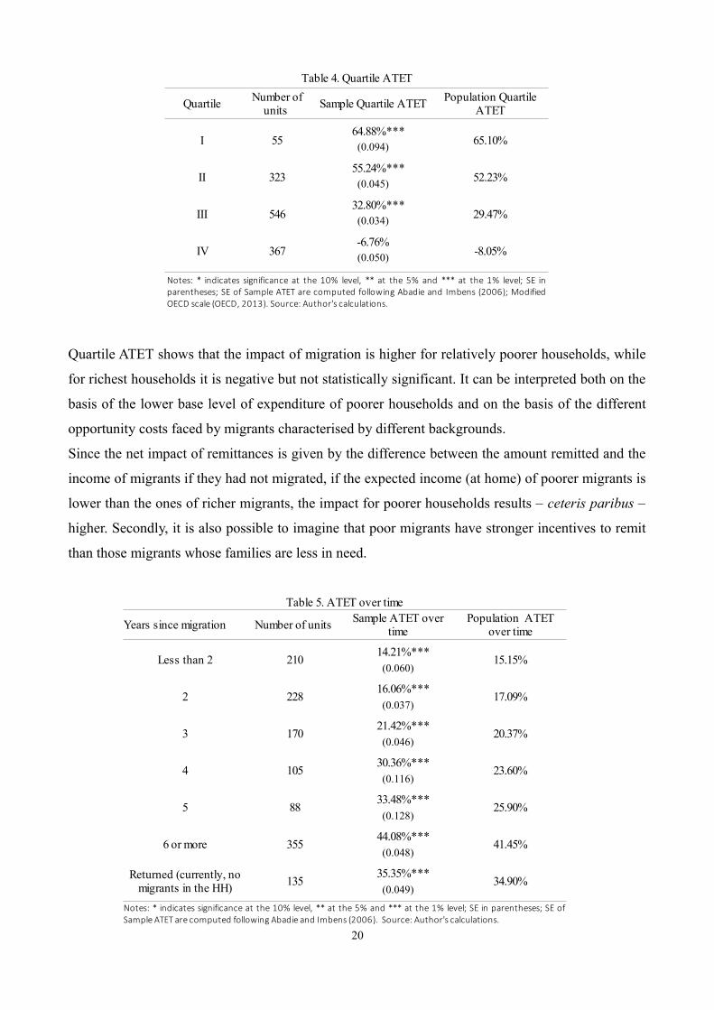
Quartile ATET shows that the impact of migration is higher for relatively poorer households, while

for richest households it is negative but not statistically significant. It can be interpreted both on the

basis of the lower base level of expenditure of poorer households and on the basis of the different

opportunity costs faced by migrants characterised by different backgrounds.

Since the net impact of remittances is given by the difference between the amount remitted and the

income of migrants if they had not migrated, if the expected income (at home) of poorer migrants is

lower than the ones of richer migrants, the impact for poorer households results – ceteris paribus –

higher. Secondly, it is also possible to imagine that poor migrants have stronger incentives to remit

than those migrants whose families are less in need.

20

Table 5. ATET over time

Years since migration Number of units

Less than 2 210 14.21%***

15.15%(0.060)

2 228 16.06%***

17.09%(0.037)

3 170 21.42%***

20.37%(0.046)

4 105 30.36%***

23.60%(0.116)

5 88 33.48%***

25.90%(0.128)

6 or more 355 44.08%***

41.45%(0.048)

135 35.35%***

34.90%(0.049)

Sample ATET over time

Population ATET over time

Returned (currently, no migrants in the HH)

Notes: * indicates significance at the 10% level, ** at the 5% and *** at the 1% level; SE in parentheses; SE of

Sample ATET are computed following Abadie and Imbens (2006). Source: Author's calculations.

Table 4. Quartile ATET

Quartile Sample Quartile ATET

I 55 64.88%***

65.10%(0.094)

II 323 55.24%***

52.23%(0.045)

III 546 32.80%***

29.47%(0.034)

IV 367-6.76%

-8.05%(0.050)

Number of units

Population Quartile ATET

Notes: * indicates significance at the 10% level, ** at the 5% and *** at the 1% level; SE in

parentheses; SE of Sample ATET are computed following Abadie and Imbens (2006); Modified

OECD scale (OECD, 2013). Source: Author's calculations.

By disaggregating the results with respect to time, it emerges that the treatment effect tends to

increase along with the length of the treatment period. This finding is consistent with the idea that

recipient households use at least part of the remittances for investment purpose and, consequently,

that remittances play a direct role in development. Indeed, if remittances were entirely spent for

consumption, the standard of living of recipient households should not grow over time. Even

though there is a series of alternative explanations that contends this interpretation (increasing remit

capacity, self-selection of successful migration experiences, consumption smoothing), their joint

explanatory power is able to account for only a part of the effect.

The estimation of counterfactual outcomes also allows to investigate the impact of migration on

social mobility and inequality. The first one has been originally captured building a transition matrix

linking migrant households' observed outcomes to their estimated counterfactuals. The matrix

shows that migration is a risky strategy but, when successful, it guarantees a great improvement of

the well-being of households' members. On average, it results that about half of migrant households

have been successful in climbing the social ladder, “migrating” to a higher expenditure quintile. On

21

Observed scenario quintile (migration)I II III IV V

I 0.5% 0.5% 0.4% 0.3% 0.7%

II 0.9% 1.7% 4.0% 4.6% 6.9%

III 0.7% 3.6% 4.5% 9.7% 11.9%

IV 1.0% 2.9% 6.7% 9.9% 13.7%

V 0.3% 2.2% 2.5% 3.7% 6.1%

Notes: Modified OECD scale (OECD, 2013); sample weights included. Source: Author's calculations.

Percentage on diagonal: 22.7%Percentage that moved up by at least one quintile (migration success): 52.6%Percentage that moved down by at least one quintile (migration failure): 24.7%

Table 6A. Variation of migrant households' ranking in the expenditure distribution: transition matrix from counterfactual (no migration) to observed scenario

Counterfactual scenario quintile (no migration)

Table 6B. Distributions of migrant households

Relative frequency of migrant HH

Observed Counterfactual Observed Counterfactual

I 3.2% 2.6% 1.6% 1.4%

II 10.6% 16.5% 5.5% 8.5%

III 18.1% 27.2% 9.3% 14.1%

IV 28.1% 37.7% 14.5% 19.5%

V 40.2% 15.9% 20.8% 8.3%Notes: Modified OECD scale (OECD, 2013); sample weights included. Source: Author's calculations.

Expenditure quintiles

Quintile to which migrant HH belong (marginal distributions of transition matrix)

the other hand, in one out of four cases migration seems to have worsened the economic condition

of the households. Finally, looking at the marginal distributions, it emerges that international

migration is a phenomenon which does not directly regards the most disadvantages sections of

Bangladesh's population. Quite the opposite, about four out of five international migrants come

from relatively better-off households while less than three percent of them originates from

household belonging to the poorest quintile. Having an emigrated member is common among

relatively wealthy families, but it's quite rare among the households belonging to the first quintile.

As far inequality, migration results to increase expenditure inequality by 1.58 Gini points. This

finding is consistent with Brown and Jimenez (2008) and Barham and Boucher (1998), even if in

this case the difference is smaller and the 95% confidence intervals of the two estimates overlap.

Moving from a positive analysis to some brief normative considerations, the results may seem to

call for development policies aimed at making the migration strategy available also to poor

households. On the contrary, the results of this study cannot be taken as evidence in support of such

policy conclusions. Firstly, nearly all of the households belonging to the lowest expenditure quintile

fall outside of the overlapping region and, consequently, the analysis has not much to say of the

effect of migration on their welfare. Secondly, as clearly emerges from Figure 1, almost none of the

relevant households' characteristics (e.g. all the variables related to the demographic structure) can

be directly influenced by governmental policies. Since Bangladesh has implemented policies aimed

at incentivizing outward migration and export of national manpower (e.g. establishing the Ministry

of Expatriates' Welfare and Overseas Employment and the Probashi Kallyan Bank, a financial

institution aimed to deliver subsidized financial services to migrants), besides the legitimate

concerns regarding the effectiveness of these institutions in achieving their official objectives, the

analysis suggests that – from a partial equilibrium perspective – the resources deployed in these

policies mostly benefit relatively better-off households.

7. Conclusions

This research explores from different perspectives the impact of international migration on the

22

Table 7. Gini indexes comparison: observed vs. counterfactualScenario Gini index Lower bound (95%) Upper bound (95%)

Observed (migration) 33.15 31.22 35.01

Counterfactual (no migration) 31.57 29.63 33.52Notes: Modified OECD scale (OECD, 2013); sample weights included. Source: Author's calculations.

welfare of Bangadeshi migrant households. The analysis indicates that, on average, migration

produces a significant and substantial positive impact on the welfare of migrants' family members, a

result which has proved to be robust to different assumptions regarding households' economies of

scale. Quartile ATET shows that the welfare effect is stronger for the households belonging to the

first quartile, while it is not statistically significant for the households belonging to the fourth.

Looking at the expenditure distribution, it emerges that households engaged in migration are

concentrated in the third and fourth quintiles, whereas less than three percent originate from the

first. This finding suggests that the direct benefits of migration and remittances are unbalanced in

favour of relatively wealthy households, even though the poorest sections of the population may

benefit from some general equilibrium effect (not estimated). In general, international migration

appears to be a household strategy characterised by high expected return and significant risk: it is a

major cause of social mobility, but is precluded to the poorest households. By adopting social

mobility as a yardstick for the success of migration, it turns out that in about half of the cases

migrant households are able to climb the social ladder but, on the other hand, one out of four

migration experiences ends up with the households falling in a lower expenditure quintile.

Migration and remittances produce also a negative effect of inequality, but it appears relatively

modest. As regards policy implications, the analysis shows that since most of the characteristics that

determine migration choices cannot be influenced by policymakers, it is likely that any policy

aimed to make migration easier, if effective, would directly benefit relatively better-off households.

References

Abadie, A., Drukker, D., Herr, J.L., and Imbens, G.W. (2004) Implementing matching estimators foraverage treatment effects in Stata. Stata journal, 4, 290-311.

Abadie, A., and Imbens, G.W. (2006) Large sample properties of matching estimators for averagetreatment effects. Econometrica, 74(1), 235-267.

Acosta, P., Calderon, C., Fajnzylber, P., and Lopez, H. (2008) What is the impact of internationalremittances on poverty and inequality in Latin America?. World Development, 36(1), 89-114.

Adams, R.H. (2011) Evaluating the economic impact of international remittances on developingcountries using household surveys: A literature review. Journal of Development Studies,47(6), 809-828.

Adams, R.H., and Cuecuecha, A. (2010) Remittances, household expenditure and investment inGuatemala. World Development, 38(11), 1626-1641.

23

Adams, R.H., and Cuecuecha, A. (2013) The impact of remittances on investment and poverty inGhana. World Development, 50, 24-40.

Adams, R.H., and Page, J. (2005) Do international migration and remittances reduce poverty indeveloping countries?. World development, 33(10), 1645-1669.

Agarwal, R., and Horowitz, A.W. (2002) Are international remittances altruism or insurance?Evidence from Guyana using multiple-migrant households. World development, 30(11), 2033-2044.

Amuedo-Dorantes, C., and Pozo, S. (2004) Workers' remittances and the real exchange rate: aparadox of gifts. World development, 32(8), 1407-1417.

Asadullah, M.N., Savoia, A., and Mahmud, W. (2014) Paths to development: is there a Bangladeshsurprise?. World Development, 62, 138-154.

Austin, P.C. (2011) Optimal caliper widths for propensity score matching when estimating‐

differences in means and differences in proportions in observational studies. Pharmaceutical

statistics, 10(2), 150-161.

Bangladesh Bank (2013) Of Changes and Transformations. Www.bb.org.bd/pub/special/chngtrnsform.pdf .

Barham, B., and Boucher, S. (1998) Migration, remittances, and inequality: estimating the neteffects of migration on income distribution. Journal of development economics, 55(2), 307-331.

Beine, M., Docquier, F., and Rapoport, H. (2001) Brain drain and economic growth: theory andevidence. Journal of development economics, 64(1), 275-289.

Bertoli, S., and Marchetta, F. (2014) Migration, remittances and poverty in Ecuador. The Journal of

Development Studies, 50(8), 1067-1089.

Borjas, G.J. (1987) Self-Selection and the Earnings of Immigrants. American Economic Review,77(4), 531-53.

Brown, R.P., and Jimenez., E. (2008) Estimating the net effects of migration and remittances onpoverty and inequality: comparison of Fiji and Tonga. Journal of International Development,

20(4), 547-571.

Calero, C., Bedi, A.S., and Sparrow, R. (2009) Remittances, liquidity constraints and human capitalinvestments in Ecuador. World Development, 37(6), 1143-1154.

Caliendo, M., and Kopeinig, S. (2008) Some practical guidance for the implementation ofpropensity score matching. Journal of economic surveys, 22(1), 31-72.

Chowdhury, M.B. (2011) Remittances flow and financial development in Bangladesh. Economic

Modelling, 28(6), 2600-2608.

Combes, J.L., Ebeke, C., Etoundi, M.N. and Yogo, T. (2014) Are foreign aid and remittance inflowsa hedge against food price shocks in developing countries? World Development, 54 (1), 81–

24

98.

Cox-Edwards, A., and Rodríguez-Oreggia, E. (2009) Remittances and labor force participation inMexico: an analysis using propensity score matching. World Development, 37(5), 1004-1014.

Deaton, A., and Zaidi, S. (2002) Guidelines for constructing consumption aggregates for welfare

analysis (Vol. 135). World Bank Publications.

Dehejia, R.H., and Wahba, S. (1999) Causal effects in nonexperimental studies: Reevaluating theevaluation of training programs. Journal of the American statistical Association, 94(448),1053-1062.

Dehejia, R.H., and Wahba, S. (2002) Propensity score-matching methods for nonexperimentalcausal studies. Review of Economics and statistics, 84(1), 151-161.

DuGoff, E.H., Schuler, M., and Stuart, E. A. (2014) Generalizing observational study results:applying propensity score methods to complex surveys. Health services research, 49(1), 284-303.

Faaland, J., and Parkinson, J.R. (1976) Bangladesh: The test case of development. C. Hurst:London.

Giannelli, G.C., and Mangiavacchi, L. (2010) Children's Schooling and Parental Migration:Empirical Evidence on the ‘Left behind’ Generation in Albania. ‐ Labour, 24(s1), 76-92.

Gibson, J., McKenzie, D., and Stillman, S. (2011) The impacts of international migration onremaining household members: omnibus results from a migration lottery program. Review of

Economics and Statistics, 93(4), 1297-1318.

Gibson, J., McKenzie, D., and Stillman, S. (2011) What happens to diet and child health whenmigration splits households? Evidence from a migration lottery program. Food Policy, 36(1),7-15.

Gibson, J., McKenzie, D., and Stillman, S. (2013) Accounting for selectivity and duration-dependent heterogeneity when estimating the impact of emigration on incomes and poverty insending areas. Economic Development and cultural change, 61(2), 247-280.

Giuliano, P., and Ruiz-Arranz, M. (2009) Remittances, financial development, and growth. Journal

of Development Economics, 90(1), 144-152.

Graham, E., Jordan, L.P., and Yeoh, B.S. (2015) Parental migration and the mental health of thosewho stay behind to care for children in South-East Asia. Social Science and Medicine, 132,225-235.

Gupta, S., Pattillo, C.A., and Wagh, S. (2009) Effect of remittances on poverty and financialdevelopment in Sub-Saharan Africa. World Development, 37(1), 104-115.

Hadi, A. (2001) International migration and the change of women's position among the left behind‐

in rural Bangladesh. International Journal of Population Geography, 7(1), 53-61.

Ham, J.C., Li, X., and Reagan, P.B. (2011) Matching and semi-parametric IV estimation, a distance-

25

based measure of migration, and the wages of young men. Journal of Econometrics, 161(2),208-227.

Hanson, G.H. (2010) International Migration and the Developing World. Handbook of Development

Economics, 5, 4363-4414.

Heckman, J.J. (1979) Sample selection bias as a specification error. Econometrica: Journal of the

econometric society, 153-161.

Holland, P.W. (1986) Statistics and causal inference. Journal of the American statistical

Association, 81(396), 945-960.

Imbens, G.W., and Rubin, D.B. (2015) Causal inference in statistics, social, and biomedical

sciences. Cambridge University Press.

Jalan, J., and Ravallion, M. (2003) Does piped water reduce diarrhea for children in rural India?.Journal of econometrics, 112(1), 153-173.

Jimenez-Soto, E.V., and Brown, R.P. (2012) Assessing the Poverty Impacts of Migrants’Remittances Using Propensity Score Matching: The Case of Tonga. Economic Record,88(282), 425-439.

Kumar, R.R., and Stauvermann, P.J. (2014) Exploring the nexus between remittances and economicgrowth: a study of Bangladesh. International Review of Economics, 61(4), 399-415.

Lartey, E.K., Mandelman, F.S., and Acosta, P.A. (2012) Remittances, exchange rate regimes and theDutch disease: a panel data analysis. Review of International Economics, 20(2), 377-395.

Lewis, D. (2011) Bangladesh: Politics, economy and civil society. Cambridge University Press.

Lokshin, M., Bontch Osmolovski, M., and Glinskaya, E. (2010) Work Related migration and‐ ‐

poverty reduction in Nepal. Review of Development Economics, 14(2), 323-332.

McKenzie, D., and Rapoport, H. (2011) Can migration reduce educational attainment? Evidencefrom Mexico. Journal of Population Economics, 24(4), 1331-1358.

Mendola, M. (2008) Migration and technological change in rural households: Complements orsubstitutes?. Journal of Development Economics, 85(1), 150-175.

Mishra, P. (2007) Emigration and wages in source countries: Evidence from Mexico. Journal of

Development Economics, 82(1), 180-199.

Möllers, J., and Meyer, W. (2014) The effects of migration on poverty and inequality in ruralKosovo. IZA Journal of Labor and Development, 3(1), 16.

Mohapatra, S., Ratha, D., and Silwal, A. (2010) Outlook for Remittance Flows 2011–12. World

Bank Migration and Development Brief, 13, 1-14.

OECD (2013) OECD Framework for Statistics on the Distribution of Household Income,

Consumption and Wealth. OECD Publishing. Http://dx.doi.org/10.1787/9789264194830-en.

Puhani, P. (2000) The Heckman correction for sample selection and its critique. Journal of

26

economic surveys, 14(1), 53-68.

Ratha, D. (2006) 'Economic Implications of Remittances and Migration', proceedings of 2nd Intl.Conference on Migrant Remittances (London, November 13, 2006)

Rosenbaum, P.R., and Rubin, D.B. (1983) The central role of the propensity score in observationalstudies for causal effects. Biometrika, 70(1), 41-55.

Siddique, A., Selvanathan, E.A., and Selvanathan, S. (2012) Remittances and economic growth:Empirical evidence from Bangladesh, India and Sri Lanka. Journal of Development Studies,48(8), 1045-1062.

Siddiqui, T. (2003) Migration as a livelihood strategy of the poor: the Bangladesh case. Refugeeand Migratory Movements Research Unit, Dhaka University.

Smith, J.A., and Todd, P.E. (2005) Does matching overcome LaLonde's critique of nonexperimentalestimators?. Journal of econometrics, 125(1), 305-353.

Stahl, C.W., and Habib, A. (1989) The Impact Of Overseas Workers'remittances On IndigenousIndustries: Evidence From Bangladesh. The Developing Economies, 27(3), 269-285.

Stark, O., and Levhari, D. (1982) On migration and risk in LDCs. Economic Development and

Cultural Change, 31(1), 191-196.

Stark, O., and Lucas, R.E. (1988) Migration, remittances, and the family. Economic Development

and Cultural Change, 465-481.

Stillman, S., McKenzie, D., and Gibson, J. (2009) Migration and mental health: Evidence from anatural experiment. Journal of health economics, 28(3), 677-687.

UNESCO (2011) World data on education, 7th edition, 2010/11 – Bangladesh.Http://unesdoc.unesco.org/images/0021/002112/211299e.pdf.

United Nations (2013) International Migration Report 2013.

Winship, C., and Morgan, S. (2007) Counterfactuals and causal inference. Cambridge UniversityPress.

Wooldridge, J.M. (2010) Econometric analysis of cross section and panel data. MIT press.

World Bank (2006) Global Economic Prospects: Economic Implications of Remittances and

Migration.

Zanutto, E.L. (2006) A comparison of propensity score and linear regression analysis of complexsurvey data. Journal of Data Science, 4(1), 67-91.

27

Appendix

28