Embed Size (px)
Citation preview
Unemployment, the Business Cycle and
Monetary Policy
Augmenting a Medium Sized New Keynesian DSGE Model
with Labor Market Dynamics
Master’s Thesis
to confer the academic degree of
Master of Science
in the Master’s Program
Economics
Author:
Alexander Koll
Submission:
Department of Economics
Thesis Supervisor:
Prof. Dr. Michael Landesmann
Assistant Thesis Supervisor:
Dr. Jochen Güntner
June 2015

1
Sworn Declaration
“I hereby declare under oath that the submitted Master's degree thesis has been written solely
by me without any third-party assistance, information other than provided sources or aids have
not been used and those used have been fully documented. Sources for literal, paraphrased and
cited quotes have been accurately credited.
The submitted document here present is identical to the electronically submitted text document”

2
Table of Contents 1. Abstract .......................................................................................................................................................... 3
2. Introduction .................................................................................................................................................... 3
3. The Christiano Eichenbaum Evans Model ..................................................................................................... 4
3.1. Empirical Estimation of a Monetary Policy Shock ........................................................................................ 4
3.2. The New Keynesian Model ............................................................................................................................ 6
3.3. Overview of the Model ................................................................................................................................... 7
3.4. Final Goods Firm ........................................................................................................................................... 8
3.5. Intermediate Goods Firms .............................................................................................................................. 8
3.6. Households ................................................................................................................................................... 11
3.7. The Wage Decision ...................................................................................................................................... 16
3.8. Monetary and Fiscal Policy .......................................................................................................................... 18
3.9. Market Clearing and Equilibrium ................................................................................................................. 18
4. The Search and Matching Model ................................................................................................................. 18
4.1. Workers ........................................................................................................................................................ 22
4.2. Firms ............................................................................................................................................................ 23
4.3. Wage determination ..................................................................................................................................... 23
5. Augmenting the CEE Model with the Search and Matching Model ............................................................ 24
5.1. The Discount Factor of Firms....................................................................................................................... 24
5.2. Firms in the DMP Framework ...................................................................................................................... 25
5.3. Wage Bargaining .......................................................................................................................................... 27
5.4. The Labor Market ......................................................................................................................................... 27
5.4.1. Intensive versus Extensive Margin ...................................................................................................... 28
5.4.2. Intermediate Goods Firms and Labor Input ......................................................................................... 28
5.5. Resource Constraint ..................................................................................................................................... 29
6. Model Simulation ......................................................................................................................................... 30
6.1. Parameter Values used for Calibration ......................................................................................................... 31
6.2. Monetary and Fiscal Policy in the NKSM Model ........................................................................................ 32
6.3. Impulse Response Functions to a Monetary Policy Shock ........................................................................... 34
6.4. Impact of Various Parameter Values on the Models Performance ............................................................... 40
6.5. Impulse Response Functions to a Technology Shock .................................................................................. 42
6.6. Further Research proposals .......................................................................................................................... 47
7. Conclusion .................................................................................................................................................... 48
A. Appendix ...................................................................................................................................................... 50
A.1. Real Marginal Cost of a Cobb-Douglas Production Technology ................................................................. 50
A.2. Log-Linearization ......................................................................................................................................... 52
A.3. The Log-Linearized System of the CEE Model ........................................................................................... 54
A.4. The Log-Linearized System of the DMP Model .......................................................................................... 60
A.5. Dynare and MATLAB Code ........................................................................................................................ 68
B. List of Figures .............................................................................................................................................. 81
C. References .................................................................................................................................................... 82

3
1. Abstract
I develop and simulate a medium sized New Keynesian DSGE model that incorporates a variant
of the Diamond Mortensen Pissarides Search and Matching model of the labor market.
Conventional New Keynesian models struggle to account for involuntary unemployment. In
contrast, the model presented here is able to capture the reaction of unemployment to a
monetary policy shock. The framework also accounts for the observed inertia and persistence
in several aggregate quantities. More work is required to improve the response of inflation in
the model.
2. Introduction
The primary motivation for this thesis is twofold. Firstly, in conventional New Keynesian
frameworks, nominal wage rigidity is the key feature to replicate the empirically observed
inertial, persistent and hump-shaped response of inflation and aggregate variables to a monetary
policy shock. I want to ascertain if staggered wage contracts are still an important friction that
is essential for the augmented model’s performance.
Secondly, fluctuations in involuntary unemployment are an integral part of the business cycle
and an unpleasant fact of everyday life. However, many macroeconomic models struggle to
account for this component. As a result, this thesis extends the now conventional New
Keynesian model developed by Christiano et al. (2005) to a more realistic framework that
incorporates involuntary equilibrium unemployment and delivers predictions for labor market
flows.
Chapter 3 and 4 describe the two models in detail. Chapter 5 explains the way the frameworks
are linked together. The only significant modification to the Christiano et al. (2005) model is
the different treatment of the labor market, which integrates the DMP model. This thesis
discusses the issues and considerations that arise in New Keynesian modelling in general, and
specifically in the combination of the two frameworks. The model presented here seeks to
combine the most plausible considerations of various papers to reach a credible solution.
Chapter 6 simulates the augmented model with respect to an expansionary monetary policy
shock, as well as a positive technology shock. 1 For this purpose, the model is calibrated using
parameter values from the existing literature. Specifically, the parameterizations provided by
Christiano et al. (2013) as well as Gertler et al. (2008) are utilized. Furthermore, the importance
of several parameters and their implications for the performance of the model are explained.
Before proceeding to the conclusion in chapter 7, a short discussion about potential future
research is provided. The appendix includes the derivations for all the important equations as
well as the respective log-linearizations. The working paper of Christiano et al. (2001) contains
any aspect of the New Keynesian model that is not described in this thesis. Moreover, the
appendix includes the complete Dynare (Adjemian, et al., 2011) and MATLAB codes needed
to replicate the simulations and the corresponding graphs used throughout this thesis.
1 Note that Christiano et al. (2005) do not discuss a technology shock.

4
3. The Christiano Eichenbaum Evans Model
This chapter explains the model and summarizes the key parts and findings of the paper written
by Christiano et al. (2005). The authors, CEE henceforth, develop and simulate a New
Keynesian model that is used to examine the combination of real and nominal rigidities that
help to replicate the empirically observed inertia and persistence in real variables in response
to a monetary policy shock
3.1. Empirical Estimation of a Monetary Policy Shock
Prior to building a model one needs to determine how macroeconomic variables actually
respond in reality. CEE describe monetary policy as
𝑅𝑡 = 𝑓(𝛀𝑡) + 𝜖𝑡, 3.1-1
where 𝑅𝑡 is the federal funds rate, 𝑓 is a linear function of the time 𝑡 information set 𝛀𝑡 and 𝜖𝑡 is the monetary policy shock. The Federal Reserve Bank is assumed to allow money growth to
be whatever is required to ensure that equation 3.1-1 holds. The maintained assumption for
identification states that 𝜖𝑡 is orthogonal to the entries in 𝛀𝑡.
The authors use an identified nine-variable vector autoregressive (VAR) model for estimating
the impulse response functions of eight major macroeconomic variables. The VAR has the
following structure:
𝒀𝑡 =𝑌1𝑡𝑅𝑡𝑌2𝑡
, 𝒀1𝑡 =
[ 𝑅𝑒𝑎𝑙 𝐺𝐷𝑃
𝑅𝑒𝑎𝑙 𝐶𝑜𝑛𝑠𝑢𝑚𝑝𝑡𝑖𝑜𝑛
𝐺𝐷𝑃 𝐷𝑒𝑓𝑙𝑎𝑡𝑜𝑟
𝑅𝑒𝑎𝑙 𝐼𝑛𝑣𝑒𝑠𝑡𝑚𝑒𝑛𝑡
𝑅𝑒𝑎𝑙 𝑊𝑎𝑔𝑒
𝐿𝑎𝑏𝑜𝑟 𝑃𝑟𝑜𝑑𝑢𝑐𝑡𝑖𝑣𝑖𝑡𝑦]
, 𝒀2𝑡 = [𝑅𝑒𝑎𝑙 𝑃𝑟𝑜𝑓𝑖𝑡𝑠
𝐺𝑟𝑜𝑤𝑡ℎ 𝑅𝑎𝑡𝑒 𝑜𝑓 𝑀2] 3.1-2
The ordering of the variables entails two key identification assumptions. Firstly, the vector 𝒀1𝑡 consists of those variables that are assumed to respond slowly to a monetary policy shock.
Therefore, they are contained in the time 𝑡 information set. Secondly, 𝒀2𝑡 contains variables
that are allowed to respond contemporaneously with a monetary policy shock and are thus not
contained in 𝛀𝑡. For this reason, only past values of 𝒀2𝑡 are included in the time 𝑡 information
set.
The choice of variables in each vector is consistent with the timing assumptions made in the
model described below. All variables, except money growth, have been transformed using the
natural logarithm but were kept in levels. Since several variables are growing over time, this
could theoretically affect the estimation results. However, CEE argue that alternative
specifications, that account for potential cointegration relationships, have been tested and that
the results are unaffected.

5
The sample period in the paper spans from the third quarter 1965 to the third quarter 1995.2
Ignoring the constant term, the VAR(4) model, as estimated by CEE, has the following form
𝒀𝑡 = 𝑨1𝒀𝑡−1 +⋯+ 𝑨4𝒀𝑡−4 + 𝑪𝜼𝑡 . 3.1-3
The vector 𝜼𝑡 is a nine dimensional zero-mean, serially uncorrelated shock with a diagonal
variance-covariance matrix. 𝑪 is a 9x9 lower triangular matrix with diagonal terms equal to
unity. The seventh element of the vector 𝜼𝑡 is the monetary policy shock denoted by 𝜖𝑡. This
results from the fact that there are six variables in 𝒀1𝑡.
Note that a contractionary monetary policy shock corresponds to a positive shock to 𝜖𝑡. The
dynamic behavior of 𝒀𝑡, after a one standard deviation shock to 𝜖𝑡, is computed by ordinary
last squares. The resulting path gives the coefficients in the impulse response functions that
CEE are interested in. The authors argue that the ordering of the variables within 𝒀𝑖𝑡 does not
alter the results.
Figure 3.1-1, taken from CEE, shows the impulse response functions of all variables
in 𝒀𝑡 following an expansionary one-standard-deviation shock in monetary policy. Lines
marked with plus signs correspond to the VAR based point estimates. Grey areas are the 95
percent confidence intervals from the VAR.3 Solid lines are the DGE model’s impulse
responses. The asterisk specifies the period in which the policy shock occurs.
Units on the horizontal axes are quarters, whereas units on the vertical axes denote percentage
deviations from the unshocked path, except for inflation, the interest rate as well as the growth
rate of money which are denoted in annualized percentage point deviations (APR) from their
unshocked path.
Based on the VAR results, CEE point out several interesting responses to an expansionary
monetary policy shock.
Output, consumption as well as investment respond in a hump-shaped manner, reaching
their peak after around one and a half years. All three variables return to pre-shock levels
roughly three years later.
Inflation also responds in a sluggish way, while reaching its peak after about two years.
The interest rate decreases for about a year.
Real profits, real wages and labor productivity rise.
The growth rate of money increases instantaneously.
2 The sample period is identical to Christiano et al. (1999). 3 Confidence intervals are calculated by the method described in Sims and Zha (1999).

6
Figure 3.1-1 Model and VAR based Impulse Responses (CEE 2005)
Table 3.1-1 Percentage Variance due to Monetary Policy Shocks (CEE 2005)
The authors remark that their estimation strategy focuses solely on the share caused by a
monetary policy shock. Table 3.1-1 seeks to explain how large that factor is in relation to the
aggregate variation in the data. With the exemption of inflation and the real wage, monetary
policy shocks appear to explain a nontrivial fraction of the variation in the variables. However,
the sizeable confidence intervals reveal that these point estimates should be interpreted with
caution. Moreover, unlike the impulse response functions discussed above, variance
decompositions are generally not insensitive to alternative specifications. This thesis abstracts
from issues that arise from potential misspecifications.
3.2. The New Keynesian Model
CEE estimate a dynamic general equilibrium model (DGE) with a mixture of five different real
and nominal rigidities. Calvo-style nominal price and wage contracts are implemented as
nominal rigidities, whereas habit formation in the utility function, convex investment
adjustment costs, variable capital utilization as well as working capital loans are considered as
The variance decompositions show how
much of the k-step ahead forecast error
variance of each of the variables in 𝒀𝑡 can be explained by the exogenous
monetary policy shock, for 𝑘 = 4, 8
and 20 quarters.
The boundaries of the associated 95%
confidence intervals are shown in
parenthesis and are calculated from the
estimated VAR via bootstrapping.

7
real rigidities. The upcoming sections explain the model economy as developed by CEE.4 Some
additional comments not provided by CEE are added whenever it facilitates the understanding
of the model.
3.3. Overview of the Model
Before explaining the parts of the model in detail, it helps to provide a crude overview of the
core elements. To facilitate the understanding of the basic structure of the model, Figure 3.3-1
sketches out how the various agents are interconnected. The following sections systematically
formulate the problems firms and households face in detail.
A representative, perfectly competitive firm produces a final consumption good that consists of
a continuum of intermediate goods, which in turn are produced by monopolists that employ
homogenous labor and capital services rented in perfectly competitive factor markets. At the
end of each period, profits generated by intermediate goods firms are distributed to a continuum
of households, who face several decisions during each period. They choose how much to
consume, how many units of capital services they accumulate and supply, how to divide their
financial assets into deposits, cash holdings, and so forth.
Figure 3.3-1 The Model Economy
4 To provide a more comprehensive picture, the description of the model combines parts from the published paper
as well as the working paper (Christiano et al., 2001).
8
3.4. Final Goods Firm
A final consumption good is produced by a representative, perfectly competitive firm that
bundles a continuum of intermediate goods, indexed by 𝑗 ∈ (0,1), using the technology
𝑌𝑡 = (∫𝑌𝑗𝑡
1𝜆𝑓
1
0
𝑑𝑗)
𝜆𝑓
, 3.4-1
where 1 ≤ 𝜆𝑓 < ∞ denotes the amount of substitutability between the different intermediate
goods, 𝑌𝑗𝑡, because 𝜆𝑓 is related to the elasticity of substitution, denoted by 휀, via the
relationship 𝜆𝑓 = 휀/(휀 − 1). Therefore, if 𝜆𝑓 = 1, the intermediate goods are perfectly
substitutable because in that case 휀 → ∞. The linear homogenous function used in equation
3.4-1 is a standard variant of the so-called Dixit-Stiglitz aggregator.5
Since the final goods producer is competitive, it takes its output price, 𝑃𝑡, as well as its input
prices, 𝑃𝑗𝑡, as given. Profit maximization thus implies the Euler equation, which describes the
optimal demand for intermediate good 𝑗,
𝑌𝑗𝑡 = (𝑃𝑡𝑃𝑗𝑡)
𝜆𝑓𝜆𝑓−1
𝑌𝑡 , 3.4-2
and the aggregate price index for the final good, which equals
𝑃𝑡 = (∫ 𝑃𝑗𝑡
11−𝜆𝑓
1
0
𝑑𝑗)
1−𝜆𝑓
. 3.4-3
3.5. Intermediate Goods Firms
Intermediate good 𝑗 is produced by a monopolistically competitive firm, which supplies a
differentiated input factor to the final goods producing firm. Capital and labor is rented in
perfectly competitive factor markets. More details about the functioning of these markets can
be found in the next section that describes the household problem. The production technology
is
𝑌𝑗𝑡 = {
𝑘𝑗𝑡𝛼 𝑙𝑗𝑡
1−𝛼 − 𝜙, 𝑖𝑓 𝑘𝑗𝑡𝛼 𝑙𝑗𝑡
1−𝛼 ≥ 𝜙
0 , 𝑜𝑡ℎ𝑒𝑟𝑤𝑖𝑠𝑒, 3.5-1
where 0 < 𝛼 < 1. Due to the Cobb-Douglas type production function, the parameter 𝛼
corresponds to the capital share used in the production process. Time 𝑡 labor and capital
services are denoted by 𝑙𝑗𝑡 and 𝑘𝑗𝑡 respectively. The parameter 𝜙 denotes fixed costs of
production. Therefore, 𝜙 > 0 and the value is set to guarantee that profits are zero in a steady-
5 This framework, named after the authors of the seminal paper written by Dixit and Stiglitz (1977), is used heavily
in economics for its appealing properties. The function is a CES production function because it exhibits constant
elasticity of substitution between the various input factors. A widely referenced source of information about this
function is the appendix in Baldwin et al. (2005).

9
state. Profits are distributed to households at the end of each period. Naturally, production only
takes place whenever fixed costs are covered, as represented by 𝑘𝑗𝑡𝛼 𝑙𝑗𝑡
1−𝛼 ≥ 𝜙.
Entry and exit is ruled out to keep the analysis technically feasible. Since profits are stochastic
and zero on average, they must be negative at times. If firms were allowed to exit, companies
must also be able to enter, otherwise the economy would end up with no firms, and thus no
production. However, once the model allows for entry, the firms cannot remain monopolists
because the apparent profit opportunities would result in firms wanting to enter the market and
exploit the profitable intermediate goods sectors. Consequently, monopoly power would vanish
and a more complicated analysis that endogenously determines entry and exit dynamics would
be necessary.
The nominal wage, 𝑊𝑡, does not have a firm specific subscript because it is chosen to be the
same across households that can reoptimize.6 Moreover, the nominal wage bill, 𝑊𝑡𝑙𝑗𝑡, must be
paid at the beginning of each period. As a result, the firms must borrow from financial
intermediaries. Repayment, denoted by 𝑊𝑡𝑙𝑗𝑡𝑅𝑡, occurs at the end of each period, where 𝑅𝑡
denotes the gross interest rate. The authors refer to this setup as working capital loans. They are
important because these loans generate a reduction in the firms’ marginal cost whenever the
interest rate drops due to an expansionary monetary policy. This in turn leads to a decline in
inflation.
Let 𝑅𝑡𝑘 be the nominal rental rate on capital. Therefore, total period 𝑡 costs for an intermediate
goods firm are 𝑆𝑡(𝑌𝑡, 𝑅𝑡𝑘,𝑊𝑡𝑅𝑡) = 𝑅𝑡
𝑘𝑘 +𝑊𝑡𝑙𝑗𝑡𝑅𝑡. Given Cobb-Douglas technology, cost
minimization implies that real marginal costs have the form
𝑠𝑡 = (
1
1 − α)1−𝛼
(1
𝛼)𝛼
(𝑟𝑡𝑘)
𝛼(𝑤𝑡𝑅𝑡)
1−𝛼, 3.5-2
where 𝑟𝑡𝑘 = 𝑅𝑡
𝑘/𝑃𝑡 and 𝑤𝑡 = 𝑊𝑡/𝑃𝑡 denote the real rental rate on capital services and the real
wage rate. As usual, capital letters correspond to nominal variables, whereas lower case letters
correspond to the respective real terms. The firms’ profits, putting aside fixed costs, are given
by the relation [𝑃𝑗𝑡/𝑃𝑡 − 𝑠𝑡 ]𝑃𝑡𝑌𝑗𝑡, where 𝑃𝑗𝑡 denotes firm 𝑗’s price.
Price-setting is assumed to follow a variation of the mechanism suggested in Calvo (1983). The
Calvo model of staggered price adjustment is probably the most popular price-setting
framework in modern macroeconomics. Only a constant, exogenously determined fraction of
firms is allowed to reoptimize its nominal price. Thus, reoptimization is independent across
firms and time and each firm faces a constant probability, 1 − 𝜉𝑝, of being able to optimize
prices. CEE assume that firms that can reoptimize its price do this before the realization of the
time 𝑡 growth rate of money.
The evident shortcoming of this theory is that firms cannot influence the timing of price
adjustments. Nonetheless, empirical evidence suggests that prices are not fully flexible. A more
realistic framework results in an inflation equation that becomes complex and hard to solve
analytically. For this reason, the Calvo model is a convenient way of generating empirically
plausible results within an operational framework. Moreover, CEE explain that one objection
to the Calvo style staggered price setting is that the standard formulation implies that inflation
6 Note that this is not an assumption but a result of the model setup as shown for example in Woodford (1996).

10
leads output, which is empirically counterfactual, as highlighted by Fuhrer and Moore (1995).
However, Gali and Gertler (2000) point out that this criticism does not apply to frameworks in
which 𝑠𝑡 represents real marginal costs rather than the output gap. Therefore, according to CEE,
this criticism of the Calvo pricing scheme does not apply to their model.
CEE interpret the Calvo price setting as capturing various costs of changing prices, such as
costs that arise from collecting data, from negotiating and communicating new prices or from
decision making itself. However, they do not allow for so-called menu cost interpretations
because they would apply to all price changes, including the ones associated with the simple
lagged inflation indexation scheme explained above. The authors reference microeconomic
evidence provided by Zbaracki et al. (2000) that suggests that expenses associated with
reoptimization are significantly more important than menu costs.
Firms that cannot reoptimize prices engage in lagged inflation indexation:
𝑃𝑗𝑡 = 𝜋𝑡−1𝑃𝑡−1 3.5-3
In other words, these firms change prices to match the past inflation rate. Therefore, the current
inflation rate is characterized by 𝜋𝑡 = 𝑃𝑡+1/𝑃𝑡. Lagged inflation indexation implies that
inflation itself becomes sticky. Given a proper choice of parameters, the model is able to
account for the empirically observed degree of serial correlation in inflation. Moreover, let ��𝑡 denote the value of 𝑃𝑗𝑡 chosen by firms that can reoptimize prices at time 𝑡. Just as in the case
of wages mentioned above, the nominal reoptimized price does not have a firm specific
subscript because it is identical across firms. The firm chooses ��𝑡 to maximize
Ε𝑡−1∑(𝛽𝜉𝑝)
𝑙𝑣𝑡+𝑙(��𝑡𝑋𝑡𝑙 − 𝑠𝑡+𝑙𝑃𝑡+𝑙)𝑌𝑗,𝑡+𝑙,
∞
𝑙=0
3.5-4
with 𝑣𝑡 being the marginal value of a dollar to the household, which is due to the assumption
of state contingent securities identical across households. Naturally, 𝑣𝑡 is outside the firms’
control and thus taken as exogenous. The lagged expectations operator, Ε𝑡−1, is conditional on
lagged growth rates of money, denoted by 𝜇𝑡−𝑙, with 𝑙 ≥ 1. This specification is used because
of the assumption that firms set ��𝑡 prior to the time 𝑡 growth rate of money.
The optimization problem maximizes 3.5-4, subject to 3.5-2 and 3.4-2 as well as
𝑋𝑡𝑙 = {
𝜋𝑡 × 𝜋𝑡+1 ×⋯𝜋𝑡+𝑙+1 𝑓𝑜𝑟 𝑙 ≥ 11 𝑓𝑜𝑟 𝑙 = 0
. 3.5-5
The reoptimized price ��𝑡 changes firm 𝑗’s profit only as long as it cannot optimize prices itself,
in which case 𝑃𝑗,𝑡+𝑙 = ��𝑡𝑋𝑡𝑙. The probability that a firm is forced to engage in lagged inflation
indexation is denoted by (𝜉𝑝 )𝑙.
The first order condition of the optimization problem reads
Ε𝑡−1∑(𝛽𝜉𝑝)
𝑙𝑣𝑡+𝑙𝑌𝑗,𝑡+𝑙(��𝑡𝑋𝑡𝑙 − 𝜆𝑓𝑠𝑡+𝑙𝑃𝑡+𝑙)
∞
𝑙=0
= 0. 3.5-6

11
In the absence of Calvo style staggered price setting, all firms can optimize prices and 𝜉𝑝 = 0.
Consequently, 3.5-6 reduces to the standard condition that firms set prices as a constant markup,
denoted by 𝜆𝑓, over marginal costs. As already shown in Calvo (1983), equation 3.4-3 can be
rewritten as
𝑃𝑡 = [(1 − 𝜉𝑝)��𝑡
11−𝜆𝑓 + 𝜉𝑝(𝜋𝑡−1𝑃𝑡−1)
11−𝜆𝑓]
1−𝜆𝑓
. 3.5-7
Log-linearization of equation 3.5-7 in real terms and slightly rearranging yields7
��𝑡 =
𝜉𝑝
1 − 𝜉𝑝(��𝑡 − ��𝑡−1). 3.5-8
Given these definitions, log-linearization of equation 3.5-6 results in
��𝑡 = Ε𝑡−1 [��𝑡 +∑(𝛽𝜉𝑝)
𝑙[(��𝑡+𝑙 − ��𝑡−𝑙−1) + (��𝑡+𝑙 − ��𝑡+𝑙−1)]
∞
𝑙=1
], 3.5-9
Equation 3.5-9 together with 3.5-8 can be combined to the inflation Phillips Curve8
��𝑡 =
1
1 + 𝛽��𝑡−1 +
𝛽
1 + 𝛽𝐸𝑡−1��𝑡+1 +
(1 − 𝛽𝜉𝑝)(1 − 𝜉𝑝)
𝜉𝑝𝐸𝑡−1��𝑡. 3.5-10
As outlined in section 3.1, one of the key identification assumptions of the VAR model is that
the price level does not respond contemporaneously with a monetary policy shock and is thus
not contained in time 𝑡 information set Ω𝑡. Under this Phillips curve specification, the time 𝑡 inflation rate does not respond to a time 𝑡 monetary policy shock either.
3.6. Households
A continuum of households face a number of decisions during each period. Unlike CEE, this
thesis uses 𝑖 ∈ (0,1) instead of 𝑗 ∈ (0,1) to avoid confusion.9 Each household decides upon
consumption versus capital accumulation and how many units of capital services to supply.
Furthermore, it acquires state contingent securities, which are conditional on whether it can
reoptimize its wage decision. These securities guarantee that households are homogenous with
respect to consumption and asset holdings. However, they are heterogeneous with respect to
the wage rate and the hours they work, as is reflected in the notation, an issue already mentioned
in section 3.5.
Households that can reoptimize wages set them according to a Calvo framework that is similar
to the one used for price setting. Households are also assumed to receive a lump sum transfer
7 Section A.2 of the appendix explains the method of log-linearization and the notation. The following derivation
is already provided here to facilitate a coherent characterization of the intermediate goods sector problem. 8 Named after the economist Alban W. Phillips, who was the first to observe and describe the short run inverse
relationship between unemployment and inflation. 9 This is done because the subscript 𝑗 already denotes firms.

12
from the monetary authority. Furthermore, they decide upon the amount of financial assets they
hold in the form of deposits with a financial intermediary or in the form of cash.
The utility function for the 𝑖𝑡ℎ household has the form10
𝛦𝑡−1𝑖 ∑𝛽𝑙 [𝑙𝑜𝑔(𝑐𝑡+𝑙 − 𝑏𝑐𝑡+𝑙−1) − 𝜓0(𝑛𝑖,𝑡+𝑙)
2+ 𝜓𝑞
𝑞𝑡+𝑙1−𝜎𝑞
1 − 𝜎𝑞]
∞
𝑙=0
, 3.6-1
where 𝑐𝑡 denotes time 𝑡 real consumption and 𝑛𝑖,𝑡 symbolizes time 𝑡 hours worked, which CEE
denote as ℎ𝑖𝑡. Since this quantity denotes labor as measured in the data, the standard notation
for employment used in the literature, 𝑛𝑡, seems more functionally adequate than ℎ𝑡.11 The
functional form implies a standard disutility of work term with 𝜓0 set to ensure a steady-state
value of labor equal to unity, thus full employment. Furthermore, 𝑞𝑡 = 𝑄𝑡/𝑃𝑡 denotes real cash
balances and 𝑄𝑡 represents nominal cash balances.12
The value for parameter 𝜓𝑞 is set to guarantee that 𝑄/𝑀 = 0.44 in steady-state, which is the
ratio of the money aggregates M1 over M2 at the beginning of the data set. 𝑀 denotes the
steady-state stock of money in the model. According to CEE, different values of 𝜓𝑞 only change
the estimate of the elasticity of money demand, 𝜎𝑝. The lagged expectation operator has the
same purpose as described in section 3.5.
The parameter 𝑏 introduces non-separability of preferences over time. In other words, an
increase in time 𝑡 consumption lowers marginal utility of current consumption and increases
marginal utility of next period’s consumption. Intuitively, old habits are hard to break and new
habits are difficult to form. This feature is called habit formation in the literature and is
essentially a statement about the behavioural pattern of individuals.
Figure 3.6-1 Habit Formation in the Utility Function
10 The representation of the utility function is different from CEE because the authors describe the functional form
of the terms separately. This thesis combines the equations to facilitate notation. 11 The Search and Matching model discussed in chapter 4 also uses 𝑛𝑖𝑡. 12 Including money in the utility function (MIU) is a frequently used framework in macroeconomics that was
initially developed by Sidrauski (1967). This setup models the opportunity costs of holding money with respect to
foregone interest payments. Therefore, the MIU term encourages households to optimize money holdings.

13
Figure 3.6-1 shows how consumption evolves over time in response to a positive monetary
policy shock. Habit formation is important for replicating the observed hump-shaped rise in
consumption. Standard utility functions conventionally used in economic models cannot
generate this pattern.
The households’ budget constraint in nominal terms has the form
𝑀𝑡+1 = 𝑅𝑡[𝑀𝑡 − 𝑄𝑡 + (𝜇𝑡 − 1)𝑀𝑡𝛼] + 𝐴𝑖,𝑡 + 𝑄𝑡 +𝑊𝑖,𝑡𝑛𝑖,𝑡 + 𝑅𝑡
𝑘𝑢𝑡��𝑡+ 𝐷𝑡 − 𝑃𝑡[𝑖𝑡 + 𝑐𝑡 + 𝑎(𝑢𝑡)��𝑡].
3.6-2
The period 𝑡 + 1 money stock of households, denoted by 𝑀𝑡+1, has to equal the sum of the
expressions on the right-hand side. Deposits held at financial intermediaries are defined as
[𝑀𝑡 − 𝑄𝑡 + (𝜇𝑡 − 1)𝑀𝑡𝛼]. These deposits earn the gross nominal interest rate 𝑅𝑡. Moreover,
𝐴𝑖,𝑡 denotes net cash flows from state contingent securities, and 𝑄𝑡 stands for nominal cash
balances. Labor income is given by 𝑊𝑖,𝑡𝑛𝑖,𝑡, whereas earnings from supplying capital services
are denoted by 𝑅𝑡𝑘𝑢𝑡��𝑡. Firm profits are represented by 𝐷𝑡, and nominal consumption is
specified as 𝑃𝑡𝑐𝑡. Lastly, 𝑃𝑡[𝑖𝑡 + 𝑎(𝑢𝑡)��𝑡] denotes the stock of installed capital, which is owned
by households and evolves according to
��𝑡+1 = (1 − 𝛿)��𝑡 + [1 − 𝜙𝑖 (
𝑖𝑡𝑖𝑡−1
− 1)2
] 𝑖𝑡. 3.6-3
In other words, next period’s physical capital stock equals the sum of current period’s capital
stock adjusted for capital depreciation, denoted by 𝛿, and current and past investment that is
transformed via a technology that adds to next period’s installed capital. CEE only discuss the
properties of this function without stating the exact functional form, as can be seen in equation
3.6-15. Thanks to my supervisor Dr. Güntner, I was able to write down an operational function
that fulfils the properties stated in CEE.
Moreover, the physical capital stock, ��𝑡, is associated with capital services via the
relationship 𝑘𝑡 = 𝑢𝑡��𝑡, with 𝑢𝑡 symbolizing the utilization rate of capital, which is effectively
a control variable of the households. Finally, (𝜇𝑡 − 1)𝑀𝑡𝛼 is a lump sum payment that the
monetary authority is assumed to pay to households. The variable 𝜇𝑡 denotes the gross growth
rate of the economy-wide per capita stock of money, 𝑀𝑡𝛼.
The budget constraint in real terms can be expressed as
𝜋𝑡+1𝑚𝑡+1 = 𝑅𝑡(𝑚𝑡 − 𝑞𝑡) +
(𝜇𝑡 − 1)𝑀𝑡𝛼
𝑃𝑡+ 𝑎𝑖𝑡 + 𝑞𝑡+𝑤𝑖𝑡𝑛𝑖𝑡 + 𝑟𝑡
𝑘𝑢𝑡��𝑡
+ 𝑑𝑡 − 𝑖𝑡 − 𝑐𝑡 + 𝑎(𝑢𝑡)��𝑡,
3.6-4
where 𝜋𝑡 = 𝑃𝑡/𝑃𝑡−1 denotes the gross inflation rate of the general price level.
Household 𝑖 is assumed to
max 𝑐𝑡, 𝑞𝑡, 𝑚𝑡+1, 𝑢𝑡, 𝑖𝑡, ��𝑡+1
utility function 3.6-1
subject to 3.6-4 3.6-5

14
Therefore, the Lagrangean has the form
ℒ = 𝛦𝑡−1
𝑖 ∑𝛽𝑙−𝑡∞
𝑙=0
{[𝑙𝑜𝑔(𝑐𝑡+𝑙 − 𝑏𝑐𝑡+𝑙−1) − 𝜓0(𝑛𝑖,𝑡+𝑙)2+ 𝜓𝑞
𝑞𝑡+𝑙1−𝜎𝑞
1 − 𝜎𝑞]
+ 𝜓𝑐,𝑡+𝑙 [𝑅𝑡+𝑙(𝑚𝑡+𝑙 − 𝑞𝑡+𝑙) +(𝜇𝑡+𝑙 − 1)𝑀𝑡+𝑙
𝛼
𝑃𝑡+𝑙+ 𝑎𝑖𝑡+𝑙+𝑞𝑡+𝑙 + 𝑤𝑖𝑡+𝑙𝑛𝑖𝑡+𝑙 + 𝑟𝑡+𝑙
𝑘 𝑢𝑡+𝑙��𝑡+𝑙 + 𝑑𝑡+𝑙 − 𝑖𝑡+𝑙
− 𝑐𝑡+𝑙 + 𝑎(𝑢𝑡+𝑙)��𝑡+𝑙 − 𝜋𝑡+𝑙+1𝑚𝑡+𝑙+1]},
3.6-6
where 𝜓𝑐,𝑡 = 𝑣𝑡𝑃𝑡 and 𝑣𝑡 denotes the marginal value of a dollar to the household, which is due
to the assumption of state contingent securities identical across households. As a result, the
Lagrange multiplier 𝜓𝑐,𝑡 denotes the marginal utility of 𝑃𝑡 units of currency.
The corresponding FOCs are given by:
𝜕ℒ
𝜕𝑐𝑡:
1
𝑐𝑡 − 𝑏𝑐𝑡−1−
𝛽𝑏
𝑐𝑡+1 − 𝑏𝑐𝑡− 𝜓𝑐,𝑡 = 0. 3.6-7
In CEEs timing convention, the equation has the form
Ε𝑡−1𝑢𝑐,𝑡 = Ε𝑡−1𝜓𝑐,𝑡, 3.6-8
where 𝑢𝑐,𝑡 denotes the marginal utility of consumption at time 𝑡. Moreover, 𝜓𝑐,𝑡 corresponds
to the value of a dollar in the current period.
Equation 3.6-9 describes the household’s FOC for nominal cash balances,
𝜕ℒ
𝜕𝑞𝑡: 𝜓𝑞𝑞𝑡
−𝛿𝑞 − 𝜓𝑐,𝑡(𝑅𝑡 − 1) = 0, 3.6-9
which holds irrespective of the realization of the contemporary money growth rate because the
cash balance decision is carried out afterwards. Hence, the marginal utility of dollar assigned
to cash balances must correspond to the marginal utility of a dollar allocated to the financial
intermediary.
𝜕ℒ
𝜕𝑚𝑡+1: Ε𝑡𝛽𝜓𝑐,𝑡+1𝑅𝑡+1 − Ε𝑡𝜓𝑐,𝑡𝜋𝑡+1 = 0. 3.6-10
Rewriting this equation results in
Ε𝑡𝛽𝜓𝑐,𝑡+1
𝑅𝑡+1𝜋𝑡+1
= Ε𝑡𝜓𝑐,𝑡,
which shows that the expected present discounted value of the cash acquired by depositing a
dollar in next period’s financial market matches the value of a dollar in the current period.

15
𝜕ℒ
𝜕𝑢𝑡: Ε𝑡−1𝜓𝑐,𝑡[𝑟𝑡
𝑘 − 𝑎′(𝑢𝑡) ] = 0. 3.6-11
Equation 3.6-11 is the Euler equation that characterizes the household’s capital utilization
decision. Accordingly, the expected marginal cost of raising the capital utilization rate must
equal the corresponding marginal benefit.
A few further remarks are necessary to determine the FOC with respect to time 𝑡 investment as
well as time 𝑡 + 1 physical capital. As already remarked in section 3.3, intermediate goods
firms employ homogenous labor and capital services rented in perfectly competitive factor
markets. The following considerations are based on lecture notes from the PHD course
“Advanced Economics” of my supervisor Dr. Güntner.
Assume that intra-temporal investment is implemented by a competitive capital goods producer
that purchases (1 − 𝛿)𝑘𝑡 at the market price, 𝑃𝑘′𝑡, obtains 𝑖𝑡 investment goods, and sells 𝑘𝑡+1
at the same market price, taking equation 3.6-3 into consideration. Since firms are also owned
by households, the same discount factor can be used and the competitive capital goods producer
maximizes
Ε𝑡−1∑𝛽𝑙
∞
𝑙=0
[𝑃𝑘′,𝑡+𝑙𝑘𝑡+𝑙+1 − 𝑃𝑘′,𝑡+𝑙(1 − 𝛿)𝑘𝑡+𝑙 − 𝑖𝑡+𝑠]
= Ε𝑡−1∑𝛽𝑙∞
𝑙=0
[𝑃𝑘′,𝑡+𝑙 (1 − 𝜙𝑖 (𝑖𝑡+𝑙𝑖𝑡+𝑙−1
− 1)2
) 𝑖𝑡 − 𝑖𝑡+𝑙].
3.6-12
Consequently, the FOC with respect to time 𝑡 investment is
𝜕ℒ
𝜕𝑖𝑡: 𝜓𝑐,𝑡 {1 + 𝜙𝑖𝑃𝑘′𝑡 [(
𝑖𝑡𝑖𝑡−1
)2
−𝑖𝑡𝑖𝑡−1
] + 𝑃𝑘′𝑡𝜙𝑖
2(𝑖𝑡𝑖𝑡−1
− 1)2
}
− 𝛽Ε𝑡−1𝑃𝑘′,𝑡+1𝜓𝑐,𝑡+1𝜙𝑖 [(𝑖𝑡+1𝑖𝑡
)3
− (𝑖𝑡+1𝑖𝑡
)2
] − 𝜓𝑐,𝑡𝑃𝑘′𝑡 = 0.
3.6-13
CEE do not explicitly state the functional form 𝐹(𝑖𝑡, 𝑖𝑡−1) that describes how the capital stock
evolves, but rather use the expression provided in equation 3.6-15. Therefore, the FOC in their
paper has the shortened, yet equivalent form
Ε𝑡−1𝜓𝑐,𝑡 = Ε𝑡−1[𝜓𝑐,𝑡𝑃𝑘′𝑡𝐹1,𝑡 + 𝛽𝜓𝑐,𝑡+1𝑃𝑘′𝑡+1𝐹2,𝑡+1], 3.6-14
where 𝐹𝑗,𝑡 is the partial derivative of 𝐹(𝑖𝑡, 𝑖𝑡−1) with 𝑗 = 1,2. This function characterizes how
current and past investment can be converted into installed capital in the following period and
is specified by
𝐹(𝑖𝑡, 𝑖𝑡−1) = [1 − 𝑆 (𝑖𝑡
𝑖𝑡−1)] 𝑖𝑡. 3.6-15
CEE only restrict the function to the following properties: 𝑆(1) = 𝑆′(1) = 0 and the
investment adjustment cost parameter 𝜂𝑘 ≡ 𝑆′′(1) > 0. The right-hand side of equation 3.6-14
states that 𝐹1,𝑡 additional units of next period’s physical capital stock ��𝑡+1 can be produced with

16
an extra unit of the investment goods, whose value is denoted by 𝑃𝑘′𝑡𝐹1,𝑡Ε𝑡−1𝜓𝑐,𝑡. Moreover,
increasing period 𝑡 investment affects next period’s quantity of installed capital by 𝐹2,𝑡+1. The
respective discounted value is given by 𝛽𝜓𝑐,𝑡+1𝑃𝑘′𝑡+1𝐹2,𝑡+1. Note that the price of investment
goods in terms of consumption is equal to unity. Hence, equation 3.6-14 states that the marginal
cost of one unit of investment corresponds to the sum of these values.
Likewise, for the FOC with respect to time 𝑡 + 1 physical capital, the household is assumed to
purchase 𝑘𝑡 in period 𝑡 − 1 at the competitive market price 𝑃𝑘′,𝑡−1. In period 𝑡, the household
rents out the capital stock at the real capital rental rate, 𝑟𝑡𝑘, and sells the depreciated capital
stock at the end of the period at the current market price 𝑃𝑘′𝑡. As a result, the respective terms
in the budget constraint read
Ε𝑡−1∑𝛽𝑙
∞
𝑙=0
𝜓𝑐,𝑡+𝑙[𝑟𝑡+𝑙𝑘 𝑢𝑡+𝑙��𝑡+𝑙 + 𝑃𝑘′,𝑡+𝑙(1 − 𝛿)��𝑡+𝑙
− 𝑃𝑘′,𝑡+𝑙−1𝑎(𝑢𝑡+𝑙)��𝑡+𝑙],
3.6-16
and hence the Euler equation for next period’s physical capital stock ��𝑡+1 has the form
𝜕ℒ
𝜕��𝑡+1: 𝛽Ε𝑡−1𝜓𝑐,𝑡+1[𝑢𝑡+1𝑟𝑡+1
𝑘 + 𝑃𝑘′,𝑡+1(1 − 𝛿) − 𝑃𝑘′,𝑡𝑎(𝑢𝑡+1)]
− Ε𝑡−1𝜓𝑐,𝑡𝑃𝑘′,𝑡 = 0. 3.6-17
To obtain the expression found in CEE, equation 3.6-17 needs to be divided by 𝑃𝑘′,𝑡. Note that
there is a typo in the equation provided in the working paper of the authors,
because 𝑃𝑘′,𝑡𝑎(𝑢𝑡+1) misses 𝑃𝑘′,𝑡. As will be shown in the appendix, this typo is irrelevant in
the log-linearization of the equation, since the term cancels out either way.
3.7. The Wage Decision
Based on Erceg et al. (2000), CEE adopt a wage setting decision that takes place between
households and a representative, competitive firm that converts labor into an aggregate labor
input, 𝑙𝑡, which is used in the intermediate goods sector, as described in section 3.5.
The following technology converts labor into the aggregated labor input
𝑙𝑡 = (∫𝑛𝑖𝑡
1𝜆𝑤
1
0
𝑑𝑖)
𝜆𝑤
, 3.7-1
where 𝑛𝑖𝑡 denotes a differentiated labor service that is supplied by household 𝑖. The CES
production function is technically identical to the one used in the final goods production, as
described in section 3.4. Therefore, the optimal demand for labor supplied by household 𝑖 equals
𝑛𝑖𝑡 = (𝑊𝑡
𝑊𝑖𝑡)
𝜆𝑤𝜆𝑤−1
𝑙𝑡, 3.7-2
17
with 1 ≤ 𝜆𝑤 ≤ ∞. The nominal price of aggregate labor is denoted by 𝑊𝑡 and related to the
wage set by the 𝑖𝑡ℎ household via the function
𝑊𝑡 = [∫ 𝑊
𝑖𝑡
11−𝜆𝑤
1
0
𝑑𝑖]
1−𝜆𝑤
. 3.7-3
Households take 𝑙𝑡 as well as 𝑊𝑡 as given. Wage setting is done in the fashion of the Calvo
price setting decision. Consequently, households face a constant probability, 1 − 𝜉𝑤, of being
capable to reoptimize their nominal wage, which is independent across time and households.
Households being unable to optimize their wage at time 𝑡 change wages to match the past
inflation rate. This is called lagged inflation indexation, as described in section 3.5. Therefore,
these wages are set as
𝑊𝑖,𝑡 = 𝜋𝑡−1𝑊𝑖,𝑡−1. 3.7-4
In line with the discussion from the price setting decision, ��𝑡 denotes the value of 𝑊𝑖𝑡 chosen
by households that can reoptimize prices at time 𝑡. This wage is identical across households
that can reoptimize.
The FOC with respect to ��𝑡 is, in real terms,
Ε𝑡−1∑(𝛽𝜉𝑤)
𝑙𝜓𝑐,𝑡+𝑙 (��𝑡𝑋𝑡𝑙𝑃𝑡+𝑙
− 𝜆𝑤2𝜓0(𝑛𝑖,𝑡+𝑙)
𝜓𝑐,𝑡+𝑙)𝑛𝑖,𝑡+𝑙 = 0,
∞
𝑙=0
3.7-5
where 𝑋𝑡𝑙 is defined just like in equation 3.5-5. CEE write 𝑧𝑛,𝑡+𝑙 instead of 2𝜓0(𝑛𝑖,𝑡+𝑙), because
they do not explicitly state the functional form of the disutility of labor term in the household
utility function 3.6-1. Similar to the findings in section 3.5, assuming fully flexible wages,
ergo 𝜉𝑤 = 0, reduces equation 3.7-5 to
��𝑡
𝑃𝑡− 𝜆𝑤
𝑧𝑛,𝑡Ε𝑡−1𝑢𝑐,𝑡
= 0. 3.7-6
Therefore, in the absence of wage rigidities, households set real wages equal to a constant
markup 𝜆𝑤, times the expected marginal rate of substitution between consumption and leisure.
Note that equation 3.6-8 was used to get from 3.7-5 to 3.7-6. The “wage Phillips curve” is
derived by log-linearizing equation 3.7-5, together with 3.7-2. Therefore,
��𝑡−1 =
𝑏𝑤(1 + 𝛽𝜉𝑤2 ) − 𝜆𝑤
𝑏𝑤𝜉𝑤𝐸𝑡��𝑡 − 𝛽𝐸𝑡��𝑡+1
− 𝐸𝑡[𝛽(��𝑡+1 − ��𝑡) − (��𝑡 − ��𝑡−1)]
−1 − 𝜆𝑤𝑏𝑤𝜉𝑤
𝐸𝑡(��𝑐,𝑡 − 𝑙𝑡),
3.7-7
where 𝑏𝑤 = (2𝜆𝑤 − 1)/[(1 − 𝜉𝑤)(1 − 𝛽𝜉𝑤)].

18
3.8. Monetary and Fiscal Policy
Unlike the standard monetary policy representation used in CEE, this thesis uses a Taylor rule
of the form
𝑅𝑡𝑅= (
𝑅𝑡−1𝑅
)𝜌𝑟
[(Ε𝑡𝜋𝑡+1𝜋
)𝜌𝜋
(𝑌𝑡𝑌)𝜌𝑌
]
1−𝜌𝑟
𝑒𝜖𝑡 , 3.8-1
where 0 ≤ 𝜌𝑟 ≤ 1 determines the central bank’s pursuit to smooth interest rates over time.13 A
value different from zero reflects interest rate inertia in the Taylor rule. Moreover, 𝜌𝜋 gauges
the central bank’s reaction to deviations of inflation from gross steady-state inflation, which is
defined by 𝜋 = 𝑃/𝑃 = 1. The parameter 𝜌𝑌 regulates the central bank’s response to deviations
of output of the final goods from steady-state output. The mean zero, identically and
independently distributed (i.i.d) random error term 휀𝑡 accounts for the monetary policy shock
described in equation 3.1-1. Please refer to section 6.2 for more details about the Taylor rule.
The government is assumed to impose non distortionary lump sum taxes. Furthermore, it
follows a Ricardian fiscal policy. Consequently, fiscal policy need not be specified and inflation
is unaffected by government actions, as CEE explain.
3.9. Market Clearing and Equilibrium
According to the authors, financial intermediaries obtain 𝑀𝑡 − 𝑄𝑡 from households and a
transfer (𝜇𝑡 − 1)𝑀𝑡 from the monetary authority. In equilibrium, 𝑀𝑡 = 𝑀𝑡𝑎, where 𝑀𝑡
𝑎 defines
the economy-wide per capita stock of money. Likewise, the variable 𝜇𝑡 denotes the gross
growth rate of 𝑀𝑡𝛼. Therefore, the total amount of money that financial intermediaries receive
is 𝜇𝑡𝑀𝑡 −𝑄𝑡.
Loan market clearing implies
𝜇𝑡𝑀𝑡 − 𝑄𝑡 = 𝑊𝑡𝑙𝑡, 3.9-1
where 𝑊𝑡𝑙𝑡 denotes the nominal wage bill, which intermediate goods producers must pay at the
beginning of each period. Consequently, these firms must borrow from financial intermediaries.
Finally, the aggregate resource constraint reads
𝑐𝑡 + 𝑖𝑡 + 𝑎(𝑢𝑡) ≤ 𝑌𝑡 . 3.9-2
4. The Search and Matching Model
As mentioned in the introduction, the frictional equilibrium unemployment model presented
here is based on papers written by Diamond (1982) as well as Mortensen and Pissarides (1994).
The underlying idea is that firms and workers are simultaneously searching for matching
counterparts in the labor market. Therefore, the literature generally refers to the model as the
Diamond-Mortensen-Pissarides Search and Matching model of unemployment (the DMP
13 Christiano et al. (2005) use this specification in their robustness tests.

19
model, hereafter). This chapter develops a standard DMP model. Any considerations regarding
the integration of the DMP model into the CEE framework are left for chapter 5.
The model seeks to explain the existence of involuntary unemployment via frictional search
unemployment. In other words, there are workers that are willing to work at the current wage
but cannot find jobs. Search efforts by workers and firms are coordinated via a so-called
matching function that determines flows from unemployment to employment. On the other
hand, current matches are destroyed with an exogenous separation probability that can be
interpreted as firing or turnover dynamics which generate flows from employment to
unemployment.
The core assumptions of the basic model are as follows:
‒ Workers and firms are heterogeneous with respect to their skills, skill requirements as
well as their location.
‒ Workers and firms are risk neutral and all have imperfect information regarding their
potential counterparts.
‒ Constant returns to scale (CRS) in production and the matching function: no need to
distinguish between firms and jobs.
‒ Free entry of firms ensures that the value of posting a vacancy is zero in equilibrium.
‒ Search is costly but each match generates a surplus that is shared between workers and
firms via generalized Nash bargaining.
‒ Workers always participate in the job market and their reservation wage is lower than
the productivity of any offered job. Thus, workers always accept the offer.
To find new workers and to hire 𝑛𝑗𝑡 employees, each firm post vacancies, denoted by 𝑣𝑗𝑡. The
total number of vacancies is calculated as 𝑣𝑡 = ∫ 𝑣𝑗𝑡𝑑𝑗1
0 and the total number of employed
workers is 𝑛𝑡 = ∫ 𝑛𝑗𝑡𝑑𝑗1
0 respectively.14 It is assumed that all unemployed workers search for a
job. Moreover, the total work force is normalized to unity. Therefore, the pool of unemployed
workers coincides with the unemployment rate, which is calculated as the difference between
unity and employment.
𝑢𝑡 = 1 − 𝑛𝑡 . 4-1
Two different timing assumptions are used in the literature. Firstly, newly employed workers
have to wait until next period before they start working. This setup is in line with the baseline
DMP model and for example used by Krause and Lubik (2007). Secondly, newly hired workers
are expected to meet with firms, to bargain and to start to work immediately in the same period.
This framework is for instance used by Gertler et al. (2008) as well as Christiano et al. (2013).
As mentioned in section 3.1, CEE’s sample period for their VAR estimations is 1965Q3-
1995Q3. The U.S. labor market has a median duration of unemployment of roughly 7 weeks in
the model’s time period (Fred Database, 2015). Christiano et al. (2013) reason that using
quarterly data is comparatively long with respect to the US unemployment duration. Therefore,
the authors argue that it seems more plausible to use their employed timing assumption.
14 This setup is identical to Krause and Lubik (2007). Moreover, equation 5.5-1 uses the same definition.
20
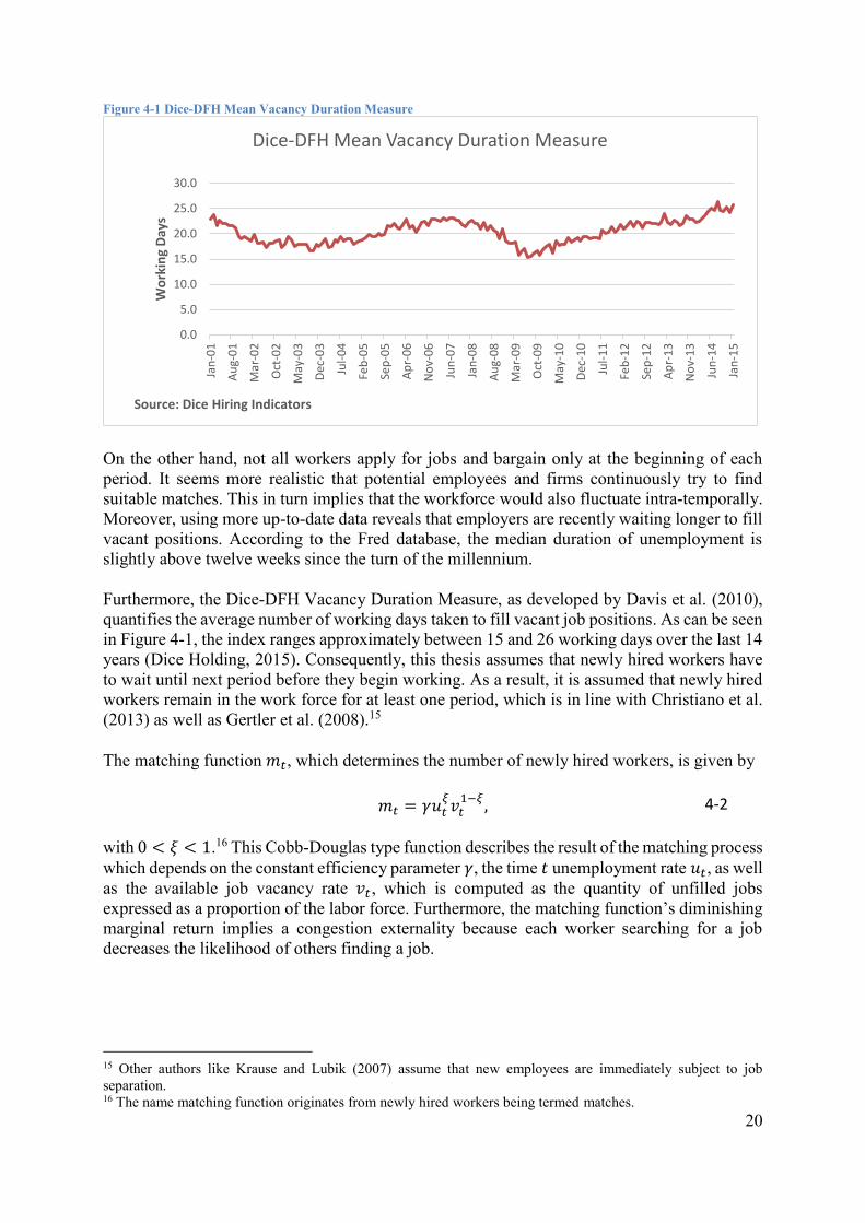
Figure 4-1 Dice-DFH Mean Vacancy Duration Measure
On the other hand, not all workers apply for jobs and bargain only at the beginning of each
period. It seems more realistic that potential employees and firms continuously try to find
suitable matches. This in turn implies that the workforce would also fluctuate intra-temporally.
Moreover, using more up-to-date data reveals that employers are recently waiting longer to fill
vacant positions. According to the Fred database, the median duration of unemployment is
slightly above twelve weeks since the turn of the millennium.
Furthermore, the Dice-DFH Vacancy Duration Measure, as developed by Davis et al. (2010),
quantifies the average number of working days taken to fill vacant job positions. As can be seen
in Figure 4-1, the index ranges approximately between 15 and 26 working days over the last 14
years (Dice Holding, 2015). Consequently, this thesis assumes that newly hired workers have
to wait until next period before they begin working. As a result, it is assumed that newly hired
workers remain in the work force for at least one period, which is in line with Christiano et al.
(2013) as well as Gertler et al. (2008).15
The matching function 𝑚𝑡, which determines the number of newly hired workers, is given by
𝑚𝑡 = 𝛾𝑢𝑡𝜉𝑣𝑡1−𝜉
, 4-2
with 0 < 𝜉 < 1.16 This Cobb-Douglas type function describes the result of the matching process
which depends on the constant efficiency parameter 𝛾, the time 𝑡 unemployment rate 𝑢𝑡, as well
as the available job vacancy rate 𝑣𝑡, which is computed as the quantity of unfilled jobs
expressed as a proportion of the labor force. Furthermore, the matching function’s diminishing
marginal return implies a congestion externality because each worker searching for a job
decreases the likelihood of others finding a job.
15 Other authors like Krause and Lubik (2007) assume that new employees are immediately subject to job
separation. 16 The name matching function originates from newly hired workers being termed matches.
0.0
5.0
10.0
15.0
20.0
25.0
30.0
Jan
-01
Au
g-0
1
Mar
-02
Oct
-02
May
-03
Dec
-03
Jul-
04
Feb
-05
Sep
-05
Ap
r-0
6
No
v-0
6
Jun
-07
Jan
-08
Au
g-0
8
Mar
-09
Oct
-09
May
-10
Dec
-10
Jul-
11
Feb
-12
Sep
-12
Ap
r-1
3
No
v-1
3
Jun
-14
Jan
-15
Wo
rkin
g D
ays
Source: Dice Hiring Indicators
Dice-DFH Mean Vacancy Duration Measure

21
Labor market tightness 𝜃, from the worker’s perspective, is defined as vacancies over
unemployment
𝜃𝑡 ≡𝑣𝑡𝑢𝑡. 4-3
The job filling rate of firms is denoted by17
𝑞𝑡 = 𝑞(𝜃𝑡) =𝑚𝑡
𝑣𝑡. 4-4
Using the matching function this can be shown to be decreasing in labor market tightness
𝑞(𝜃𝑡) = 𝑚𝜃𝑡−𝜉 , 4-5
with – 𝜉 being the elasticity of the job filling rate with respect to the labor market tightness,
defined as 𝜕𝑞𝑡
𝜕𝜃𝑡
𝜃𝑡
𝑞𝑡.
On the other hand, the job finding rate of workers is increasing in labor market tightness
𝑓𝑡 = 𝜃𝑡𝑞(𝜃𝑡) =𝑚𝑡
𝑢𝑡= 𝑚𝜃𝑡
1−𝜉 . 4-6
Both the job finding and the job filling rate depend on aggregate variables and are thus taken
as given by individual firms and workers and can be interpreted as probabilities.
The law of motion for employment is described by the function
𝑛𝑡 = (1 − 𝜌)𝑛𝑡−1 + 𝑥𝑡−1𝑛𝑡−1, 4-7
where 𝑛𝑡 denotes employment and 𝜌 the exogenous job separation rate. The presumed stability
of job separations is based on findings by Hall (2005) and Shimer (2005), who argue that the
job separation rate is relatively acyclical, or weakly countercyclical. Hall explains that it is a
common, yet erroneous belief that the sharp rise of unemployment during recessions were the
consequence of increased job separation rates. In fact, unemployment increases mainly because
of reduced hiring rates during downturns and changes in the job separation rate are miniscule
relative to the observed movements in employment.
Moreover, Shimer (2005) deduces that a time varying job separation cannot be important
because it would imply a positively sloped Beveridge curve, which plots the relationship
between the unemployment and the vacancy rate.18 The latter is typically depicted on the
vertical axes. Empirically, the Beveridge curve is negatively sloped, which suggests that high
unemployment rates are generally accompanied by a low vacancy rate, and vice versa.
As a result of the stable job separation rate, fluctuations in unemployment are due to cyclical
variation in hiring in this model. Moreover, workers who lose their job are not allowed to search
17 The job filling rate is also called the job matching rate in the literature. 18 The curve is named after the economist William H. Beveridge.

22
for a new occupation until the next period. The hiring rate is defined as the ratio of new hires
to the existing workforce
𝑥𝑖𝑡 =𝑞𝑡𝑣𝑖𝑡 𝑛𝑖𝑡
. 4-8
Given this setup, the hiring rate is effectively a firm’s control variable since the likelihood that
each posted vacancy will be filled is known to be the job filling rate 𝑞𝑡. Note that the firm’s
problem is equivalent to choosing how many vacancies to post, since one implies the other.
Moreover, using the definition of the hiring rate together with the job matching rate, equation
4-7 can be rewritten as
𝑛𝑡 = (1 − 𝜌)𝑛𝑡−1 +𝑚𝑡−1. 4-9 4.1. Workers
The worker’s choices depend on the value of employment in period 𝑡 which equals19
𝐻𝑡 = 𝑤𝑡 + Ε𝑡𝛽[(1 − 𝜌)𝐻𝑡+1 + 𝜌𝐼𝑡+1]. 4.1-1
The real wage, denoted by 𝑤𝑡, is the result of the Nash Bargaining process described below.
The term in parenthesis describes the expected discounted value of being employed or
unemployed in period 𝑡 + 1, weighted by the relevant probabilities.
The value of being unemployed is given by20
𝐼𝑡 = 𝑜 + Ε𝑡𝛽[𝑓𝑡𝐻𝑡+1 + (1 − 𝑓𝑡)𝐼𝑡+1], 4.1-2
with 𝜊 being the worker’s outside option which can be interpreted as an umbrella term for all
sorts of different non-market activities and options considered in the literature.21 Since the
outside option is constant in this thesis, no exact interpretation is provided. Otherwise, all
possible explanations would always have to exactly offset each other. As explained in section
3.8, the government is assumed to impose non distortionary lump-sum taxes. Insofar, fiscal
policy need not be specified, as CEE explain.
Section 6.4 explains the importance of the outside option for the model’s performance. A more
detailed discussion of the labor market in general can be found in section 5.4. As before, the
expression in parenthesis of equation 4.1-2 describes the expected discounted value of being
employed or unemployed in period 𝑡 + 1. This time, weighted by the job finding rate and its
complement, respectively.
19 The capital letter 𝐻 was chosen because 𝑁 already denotes employment and 𝐿 denotes the aggregate labor input
as used in the intermediate goods production process. Therefore, the value of employment is denoted as 𝐻 to avoid
confusion. It helps to think of 𝐻 as standing for “hired”, thus denoting the value of being hired. 20 The capital letter 𝐼 was used because 𝑈 already denotes unemployment. 𝐼 can be interpreted as idleness. 21 For instance, the outside option can be understood as the disutility of working (Lubik, 2009), the value of home
production (Walsh & Ravenna, 2007), the value of being unemployed (Christiano et al., 2013) or the value of
leisure (Shimer, 2005).

23
4.2. Firms
Firms can post vacancies (or job openings, positions) at a constant cost 𝜅 per period and
vacancy. The value of a vacancy is therefore given by
𝑃𝑡 = −𝜅 + Ε𝑡𝛽[𝑞(𝜃𝑡)𝐽𝑡+1 + (1 − 𝑞(𝜃𝑡))𝑃𝑡+1], 4.2-1
with the weight 𝑞(𝜃𝑡) being the aforementioned job matching rate, or the probability of filling
a job. The value of job 𝐽 is described via the relationship
𝐽𝑡 = 𝐴𝑡 − 𝑤𝑡 + Ε𝑡𝛽[(1 − 𝜌)𝐽𝑡+1 + 𝜌𝑃𝑡+1], 4.2-2
where 𝐴𝑡 is the productivity of firms. Constant returns to scale in the production function as
well as the matching function imply that this relationship can also be interpreted as the value of
a firm. The value of next period’s job 𝐽𝑡+1 is weighted by the probability of still having a job in
that period, denoted by 1 − 𝜌. Likewise, the value of posting a vacancy in period 𝑡 + 1 is
weighted by the probability of being laid-off (the job separation rate). This accounts for the fact
that unemployed people increase the value of a vacancy for firms.
Free entry of firms ensures that, in equilibrium, no producer can generate excess returns. Hence,
the value of posting a vacancy must be zero (𝑃𝑡 = 0) and 4.2-1 can be rewritten as
𝜅
𝑞(𝜃𝑡)= Ε𝑡𝛽𝐽𝑡+1, 4.2-3
where 1/𝑞(𝜃𝑡) = 𝑣𝑡/𝑚𝑡 can be interpreted as the expected duration of a posted vacancy.
Combining this with 4.2-2, again using 𝑃𝑡 = 0, yields the job creation condition
𝜅
𝑞(𝜃𝑡)= Ε𝑡𝛽 [𝐴𝑡+1 − 𝑤𝑡+1 + (1 − 𝜌)
𝜅
𝑞(𝜃𝑡+1)]. 4.2-4
The equality in 4.2-4 states that 𝜅/𝑞(𝜃𝑡) , the expected cost of posting a vacancy, equals the
expected benefit from a filled vacancy. Further considerations are left unexplained in this
section. Refer to section 5.2 for a complete treatment of the firms in the DMP model within the
CEE framework.
4.3. Wage determination
The equilibrium real wage 𝑤𝑡 is the outcome of an axiomatic Nash Bargaining process that
maximizes the generalized Nash product denoted by
max𝑤𝑡
(𝐽𝑡 − 𝑃𝑡)1−𝜂(𝐻𝑡 − 𝐼𝑡)
𝜂 , 4.3-1
with 𝜂 being the workers bargaining power, or the share of the joint surplus that goes to the
workers.22 The final solution to this bargaining process is
𝑤𝑡 = 𝜂(𝐴𝑡 + 𝜅𝜃𝑡) + (1 − 𝜂)𝑜. 4.3-2
22 The solution method is named after the mathematician John Forbes Nash, Jr.

24
As a result, the real wage is the weighted average of productivity, labor market tightness and
the outside option of workers. Moreover, by the definition of the labor market tightness, the
more firms look for workers (the higher 𝑃𝑡, given 𝐼𝑡) or the fewer workers look for jobs (the
lower 𝐼𝑡, given 𝑃𝑡), the higher the wage the worker can get.
5. Augmenting the CEE Model with the Search and Matching Model
There are five points of contact that link the two models together. The first point is the redefined
discount factor of firms in the DMP model. The second point regards the way the firm problem
is formulated in the DMP model in order to introduce output, which is neglected in traditional
Search and Matching frameworks. This also slightly changes the wage bargaining process,
which is the third point of contact. The fourth point regards the DMP firms producing the
aggregate labor input that is used in the intermediate goods production process. The final point
of contact concerns the resource constraint.
The augmented model is known as the New Keynesian Search and Matching model in the
literature, or NKSM model for short. This chapter discusses the issues and considerations that
arise in New Keynesian modelling in general, and specifically in the combination of the two
models. Overall, several related, yet competing frameworks exist and more research is needed
to determine the preferable model. The model presented here seeks to combine the most
plausible considerations of various papers to reach a credible solution.
The first papers incorporating DMP frameworks into DSGE models date back to Merz (1995)
and Andolfatto (1996). However, both papers used Real Business cycle models instead of New
Keynesian DSGE models. Seminal papers that combine contemporary New Keynesian models
with Search and Matching frameworks are Walsh (2003), Krause and Lubik (2007), Gertler et
al. (2008) and Christoffel et al. (2009). Furthermore, Christiano et al. (2013) build a model that
uses a setup of the labor market that is close to the one considered in this thesis.
Contrary to CEE, Gertler et al. (2008) assume that final goods producers are monopolistically
competitive, whereas intermediate goods producers (wholesalers in Gertler et al.) are assumed
to be competitive. This circumvents bargaining spillovers amid employees, which is needed
because Gertler et al. (2008) incorporate the labor market directly into the intermediate goods
producers’ problem. More details can be found in the authors’ paper. Due to the separated labor
market in CEE, there is no need to worry about bargaining spillovers in this framework, despite
monopoly power of intermediate goods producers.
The question of which of the two variants is more realistic remains unanswered in this thesis,
which attempts to change as little as possible from the CEE model. As a result, it assumes that
the labor market is separated from the intermediate goods sector.
5.1. The Discount Factor of Firms
The first point of contact arises via a redefined discount factor of the firms operating in the
DMP model, which is now given by
Ε𝑡𝛽 (
𝑈𝑐,𝑡+1𝑈𝑐,𝑡
) = Ε𝑡𝛽 (𝜓𝑐,𝑡+1
𝜓𝑐,𝑡), 5.1-1

25
where 𝑈𝑐,𝑡 denotes the marginal utility of consumption from the CEE model. This construction
of a stochastic pricing Kernel is consistent with other general equilibrium models that account
for labor market variables.23
The original DMP framework does not model production because the main interest lies in
employment dynamics. In this thesis, companies operating in the DMP part of the model
economy bundle the workforce to a homogenous aggregate labor input using the following
production function24
𝑙𝑗𝑡 = 𝐴𝑡𝑛𝑗𝑡 . 5.1-2
Therefore, technology is linear in labor input and driven by an aggregate labor augmenting
technology shock that is identical to all firms. This shock follows the stationary law of motion
𝐴𝑡 = 𝐴𝑡−1𝜌
𝐴1−𝜌eϵt , 5.1-3
with 𝜖𝑡 ∼ 𝑁(0, 𝜎𝜖2) and 𝜌 < 1 being the degree of autocorrelation. A more detailed discussion
of technology shocks can be found in section 6.5.
Given the linear production function, firms are indifferent to the quantity of labor hired at a
given wage rate. Due to the separation of the labor market and the intermediate goods producers
in the CEE model, there is only a small change to the Nash bargaining setup used in the standard
DMP model, which is due to a modification in the marginal product of a worker.
5.2. Firms in the DMP Framework
Recall from section 3.5 that intermediate goods firms rent labor and capital in perfectly
competitive factor markets. Consequently, each labor market firm faces a perfectly elastic
demand curve and the market price for the aggregate labor input used in the intermediate goods
production process, denoted by 𝑃𝑡𝑤, is taken as given by individuals.
The equilibrium capacity of the labor output of a single labor market firm will be entirely
determined by the quantity of output the firm decides to supply. Therefore, equation 5.1-2
represents the output constraint, which can be written as
𝐴𝑡𝑛𝑗𝑡 ≥ 𝑙𝑗𝑡 , 5.2-1
where the left-hand side characterizes the potential maximum output of the homogenous
aggregate labor input, because 𝑛𝑗𝑡 corresponds to the labor force as measured in the data. As
usual, profits are calculated as revenues (𝑃𝑡𝑤/𝑃𝑡 )𝑙𝑗𝑡 minus costs, which consist of the real wage
bill 𝑤𝑗𝑡𝑛𝑗𝑡 and vacancy posting costs 𝑘𝑣𝑗𝑡.
23 Examples of papers that employ this setup are Christiano et al. (2013), Lubik (2009) or Gertler et al. (2008).
More details about the usefulness of a stochastic discount factor can be found in Hansen and Renault (2010). 24 Eventually, all 𝑗 subscripts can be erased due to the fact that constant returns to scale in the DMP firms
production and matching functions imply that there is no need to distinguish between firms. Recall that subscript 𝑗 is used to denote firms, whereas subscript 𝑖 characterizes households. Thus, 𝑛𝑗𝑡 = 𝑛𝑖𝑡 must hold in equilibrium.

26
As a result, the intertemporal profit maximization problem of labor market firms has the
following form:
max
𝑙𝑖𝑡, 𝑛𝑡, 𝑣𝑖𝑡𝐸0∑𝛽𝑡
𝜓𝑐,𝑡
𝜓𝑐,0
∞
𝑡=0
[(𝑃𝑡𝑤
𝑃𝑡) 𝑙𝑗𝑡 − 𝑤𝑗𝑡𝑛𝑗𝑡 − 𝑘𝑣𝑗𝑡]. 5.2-2
Consequently, the Lagrangean becomes
ℒ = 𝐸0∑𝛽𝑡
𝜓𝑐,𝑡
𝜓𝑐,0
∞
𝑡=0
[(𝑃𝑗𝑡𝑤
𝑃𝑡) 𝑙𝑗𝑡 − 𝑤𝑗𝑡𝑛𝑗𝑡 − 𝑘𝑣𝑗𝑡]
+ 𝐸0∑𝛽𝑡𝜓𝑐,𝑡
𝜓𝑐,0
∞
𝑡=0
𝑚𝑐𝑗𝑡𝑤[𝐴𝑡𝑛𝑗𝑡 − 𝑙𝑗𝑡]
+ 𝐸0∑𝛽𝑡𝜓𝑐,𝑡
𝜓𝑐,0
∞
𝑡=0
𝜇𝑗𝑡[(1 − 𝜌)𝑛𝑗𝑡−1 + 𝑞(𝜃𝑡−1)𝑣𝑗𝑡−1 − 𝑛𝑗𝑡],
5.2-3
where the Lagrange multiplier 𝜇𝑗𝑡 denotes the value of a job, as will be explained below. For
the second constraint, equation 4-4 was used to rewrite the employment accumulation equation,
denoted by equation 4-9. Note that marginal costs act as a Lagrange multiplier in this setup.25
This is feasible because the contribution of an additional unit of output to the firm’s revenue
equals marginal costs.
The FOCs have the following form:
𝜕ℒ
𝜕𝑙𝑖𝑡: 𝑃𝑗𝑡𝑤
𝑃𝑡= 𝑚𝑐𝑗𝑡
𝑤 5.2-4
𝜕ℒ
𝜕𝑛𝑖𝑡: 𝑤𝑡 = 𝑚𝑐𝑗𝑡
𝑤𝐴𝑡 − 𝜇𝑗𝑡 + (1 − 𝜌)𝐸𝑡𝛽𝜓𝑐,𝑡+1
𝜓𝑐,𝑡𝜇𝑗𝑡+1 5.2-5
𝜕ℒ
𝜕𝑣𝑖𝑡: 𝜅 = 𝐸𝑡𝛽
𝜓𝑐,𝑡+1
𝜓𝑐,𝑡𝜇𝑗𝑡+1𝑞(𝜃𝑡) 5.2-6
The third FOC can be rewritten as
𝜅
𝑞(𝜃𝑡)= 𝐸𝑡𝛽
𝜓𝑐,𝑡+1
𝜓𝑐,𝑡𝜇𝑗𝑡+1.
Moreover, following the discussion of footnote 24, all 𝑗 subscripts can be erased. Therefore,
∫ 𝜇𝑗𝑡𝑑𝑗 = 𝐽𝑡1
0, denotes, just like in the standard DMP model, the value of all firms.
25 The notation 𝑚𝑐𝑖𝑡
𝑤 was chosen to distinguish these marginal costs from the ones in the New Keynesian baseline
model.

27
Given this consideration, the third FOC can be rewritten as
𝜅
𝑞(𝜃𝑡)= 𝐸𝑡𝛽
𝜓𝑐,𝑡+1
𝜓𝑐,𝑡𝐽𝑡+1, 5.2-7
which equals equation 4.2-3, except for the marginal cost term and the stochastic discount
factor, which links the NK model to the DMP model, as described above.
The second FOC can be rewritten as
𝐽𝑡 = 𝑚𝑐𝑡
𝑤𝐴𝑡 − 𝑤𝑡 + (1 − 𝜌)𝐸𝑡𝛽𝜓𝑐,𝑡+1
𝜓𝑐,𝑡𝐽𝑡+1. 5.2-8
Apart from the aforementioned linkages between the models, this equation is identical to the
value of a job as described by equation 4.2-2.
The first FOC simply states that marginal costs equal marginal revenue, which due to perfect
competition equals the (real) price 𝑃𝑡𝑤/𝑃𝑡 that firms can charge for the labor input sold to
intermediate goods producers. As a result,
𝑝𝑡𝑤 = 𝑚𝑐𝑡
𝑤, 5.2-9
where 𝑚𝑐𝑡𝑤 is given by equation 5.2-8. Forwarding 5.2-8 by one period and inserting it into the
second FOC yields the following job creation condition which resembles equation 4.2-4:
𝜅
𝑞(𝜃𝑡)= 𝐸𝑡𝛽
𝜓𝑐,𝑡+1
𝜓𝑐,𝑡[𝑚𝑐𝑡+1
𝑤 𝐴𝑡+1 − 𝑤𝑡+1 + (1 − 𝜌)𝜅
𝑞(𝜃𝑡+1)]. 5.2-10
5.3. Wage Bargaining
Wage bargaining is done according to the standard Nash bargaining framework described in
section 4.3. There is only one difference to the canonical Search and Matching model, namely
that equation 5.2-8, includes the marginal cost term, which in turn influences the marginal
product of a worker. Therefore, the wage rate is determined by the following relation
𝑤𝑡 = 𝜂𝑚𝑐𝑡𝑤𝐴𝑡 + 𝜂𝜅𝜃𝑡 + (1 − 𝜂)𝑜. 5.3-1
All other considerations are identical to section 4.3. The derivation can be found in subsection
A.4.9 of the appendix.
5.4. The Labor Market
The fourth point of contact is in the perfectly competitive labor market where intermediate
goods firms rent labor just like in the CEE setup. Overall, the household problem in the
combined model is almost identical to the one discussed in the CEE model, except that
employment is no longer a choice variable. The following subsection discusses several
considerations that are worth noting.
28
5.4.1. Intensive versus Extensive Margin
In the CEE setup, the household utility function includes a disutility of labor term. As a result,
the model does not generate movements in unemployment but voluntary movements in hours
worked. This optimization process is a common approach in standard DSGE models and is
called adjustment on the intensive margin in the literature. However, Barro’s critique (1977)
states that deviations on the intensive margin take place in long lasting relationships between
workers and firms. In theory, such interactions provide many ways of undoing the effects of
staggered nominal wage contracting. Further discussions of this issue can be found in Christiano
et al. (2008) as well as Shimer (2008).
On the other extreme, employment adjusts solely with regard to the extensive margin. This can
be modelled via the standard DMP model, since households simply accept the outcome of the
bargaining and matching process. As a result, the utility function does not include disutility of
labor anymore. Other authors like Lubik (2009) allow for a mixture of the two extreme cases.
In Lubik’s variation, the hiring decision is still subject to rigidity due to the Search and
Matching framework. Yet, the decision on how many hours to supply is fully flexible. In this
setup, the utility function still contains a disutility of labor term. However, the resulting
optimization problem is only between the present workforce and the firm.
Allowing for both variations intuitively seems to be the most plausible structure. However,
Gertler et al. (2008) suggest that most of the cyclical variation in hours is on the extensive
margin and that the intensive margin seems to play an insignificant role over the business cycle.
Likewise, empirical studies found a low overall elasticity of labor supply with respect to the net
wage rate.26 Therefore, it seems reasonable to follow Gertler et al. (2008) by assuming that only
the extensive margin matters.
5.4.2. Intermediate Goods Firms and Labor Input
Just like in CEE, the nominal wage bill for firm 𝑗, this time denoted by 𝑃𝑗𝑡𝑤𝑙𝑗𝑡, has to be paid in
advance. Consequently, the firm must borrow the amount at the current interest rate. The loan
is repaid after the firms collect their sales revenues at the end of each period. Refer to section
3.5 for a detailed explanation of the advantage of this setup in the context of the standard CEE
model.
A monopolist manufactures the intermediate good 𝑗 according to a Cobb-Douglas production
function of the form
𝑌𝑗𝑡 = {
𝑘𝑗𝑡𝛼 𝑙𝑗𝑡
1−𝛼 − 𝜙, 𝑖𝑓 𝑘𝑗𝑡𝛼 𝑙𝑗𝑡
1−𝛼 ≥ 𝜙
0 , 𝑜𝑡ℎ𝑒𝑟𝑤𝑖𝑠𝑒. 5.4.2-1
26 Blundell (1992) provides an excellent survey of papers in that subfield of economics. In general, the empirical
studies found a low overall elasticity (total effect) of labor supply with respect to the net wage rate, which suggest
that the compensated wage elasticity (the substitution effect) and the income elasticity (income effect)
approximately offset each other.

29
However, this time 𝑙𝑗𝑡 denotes the time 𝑡 aggregate labor service purchased at the competitive
price from the DMP firms.27 The competitive price 𝑃𝑗𝑡𝑤 equals the marginal costs of the DMP
firms.
The aggregate amount of the homogeneous labor input, denoted by 𝑙𝑡, is calculated according
to
𝑙𝑡 = ∫ 𝑙𝑗𝑡𝑑𝑗
1
0
. 5.4.2-2
Note that this does not denote the total labor force as measured in the data. This problem is
identical to CEE. Refer to section 5.5 for more details. Furthermore, this relationship also
represents the market clearing condition for the DMP sector.
5.5. Resource Constraint
The fifth and final point is regarding the resource constraint that specifies the division of the
homogenous final goods in the economy. In addition to the standard resource constraint used
in CEE, vacancy posting costs need to be taken into account. These cannot already be
considered on the DMP labor market level because no consumption takes place in this stage of
production. Moreover, the Search and Matching framework now determines the aggregate
amount of the homogeneous labor input used in the intermediate goods production process. Just
like in CEE, total output needs to be related to total labor as measured in the data, calculated as
𝑛𝑡 = ∫ 𝑛𝑖𝑡𝑑𝑖.
1
0
5.5-1
Using this with equations 5.1-2 and 5.4.2-2 yields the modified resource constraint given by
𝑐 + 𝑖 + 𝑎(𝑢)�� + 𝜅𝑣 ≤ (𝑃∗
𝑃)
𝜆𝑓𝜆𝑓−1
𝑘𝛼(𝐴𝑛)1−𝛼. 5.5-2
The log-linearized resource constraint has the form
[1
𝛽− (1 − 𝛿)]
𝑠𝑘𝑠𝑐��𝑡 + ��𝑡 +
𝛿𝑠𝑘𝑠𝑐
𝑖𝑡 +𝑠𝜅𝑣𝑠𝑐
��𝑡 =𝛼
𝑠𝑐��𝑡 +
1 − 𝛼
𝑠𝑐(��𝑡 + ��𝑡), 5.5-3
where all variables are defined as in CEE and the additional term 𝑠𝜅𝑣 = 𝜅𝑣/𝑌. The exact steps
in the log-linearization of the resource constraint are provided in the appendix.
27 In this case, the parameter 𝛼 corresponds to the capital share used in the production process, whereas the
parameter 1 − 𝛼 is not the labor share, which partially depends on the outcome of the bargaining process described
in section 4.3.

30
6. Model Simulation
CEE distinguish between three groups of parameters in their paper. The first group of
parameters is calibrated in a way that guarantees plausible steady-state values for the affected
variables. The second group of parameters characterizes monetary policy, whereas the third
group is assessed by minimizing a measure of the gap between the model and the empirical
impulse response functions.28
Other authors like Christiano et al. (2013) use a Bayesian estimation strategy with a
considerable larger data set that covers the period 1951Q1 to 2008Q4. The authors estimate
various model specifications, including one that uses a Nash Bargaining search setup that is
similar to the one described in this thesis. Furthermore, Gertler et al. (2008) also use the same
quarterly series in combination with a Bayesian estimation strategy. Their sample period in the
paper goes from 1960Q1 to the 2005Q1. Among other setups, they also estimate a model that
uses a Nash Bargaining framework that is comparable to the one applied here.
Replicating any of the procedures described above goes beyond the scope of this thesis.
Therefore, the estimated parameter values from the aforementioned papers are used for
calibrating the model presented here. Needless to say, this approach is inferior to estimating the
parameters for this specific model. However, this task would significantly extend the workload.
Therefore, this tactic is used for the sake of brevity.
Five different models are simulated and compared in this chapter. Initially, the standard CEE
model, which serves as the benchmark model, is considered. Moreover, the benchmark model
with fully flexible wages is simulated as well. This is done to obtain impulse response functions
that highlight the importance of the staggered wage setting framework for the benchmark
model, as pointed out by CEE. The third model is the New Keynesian Search and Matching
(NKSM) model as developed in this thesis, simulated with the original parameter values from
the benchmark model. The additional parameters that arise from the DMP framework are taken
from Christiano et al. (2013). This version is abbreviated as NKSM CEE model.
Initially, using standard estimates from conventional DMP models was considered as well.
However, the NKSM model derived in this thesis uses fully flexible wages. Hall (2005) and
Shimer (2005) were the first to show that these parameter values require sticky wages in the
DMP framework to produce empirically plausible results. As discussed in chapter 5, the
incorporation of the DMP model into a New Keynesian model also changes the structure of the
DMP framework. For this reason, estimated values from Christiano et al. (2013) are used for
the DMP part of the model because the authors assume a link between the intermediate goods
and labor market sectors that is similar to the framework discussed here. The fourth model,
NKSM CET model for short, uses the entire set of parameters as estimated by Christiano et al.
(2013). Parameter values from Gertler et al. (2008) are employed for calibrating the fifth
variant, abbreviated as NKSM GST model.
The different models are solved and simulated with the Dynare software package (Adjemian,
et al., 2011), that is run on top of MATLAB.29
28 This procedure is called impulse response function matching. 29 The appendix includes all Dynare and MATLAB files as well as the complete log-linearized system of equations.
Specifically, Dynare version 4.4.3 and MATLAB R2014a are used.

31
6.1. Parameter Values used for Calibration
The specific timing assumption of CEE, in which the lagged expectations operator Ε𝑡−1 is used,
is not applied in this thesis. The reason is that no separate VAR model is estimated and the
differences between frictionless labor markets, sticky wages and Search & Matching frictions
can in principle be evaluated for any consistent timing assumption.
Since the other papers discussed in this thesis, apply a more conventional timing assumption
with a standard contemporaneous expectations operator, Ε𝑡, this setup is used throughout the
text. Note that CEE explain in the Journal of Political Economy (2005) that their timing
assumptions ensure consistency with the identification assumption of the VAR. However, the
authors also show that the impact of changing the timing assumptions is marginal. Despite
minor differences that favor the benchmark model, the changes are negligible for the purpose
of this thesis.
Table 6.1-1 summarizes the various parameter values used for calibration. Note that CEE re-
estimate the flexible wage model with the identical parameters as used in the benchmark
model.30 Most parameter values are taken directly from the papers. CET stands for Christiano
et al. (2013). The value of the workers outside option was taken from Hagedorn and Manovskii
(2008) because CET use a time varying measure. Moreover, Gertler et al. (2008) is abbreviated
as GST. The authors do not provide vacancy posting costs. For this reason, the value of Shimer
(2005) is used instead.
Table 6.1-1 Parameter Estimates for Calibration
30 CEE utilize slightly different parameter values in the Journal of Political Economy (2005) than in the working
paper (2001). These values are also provided in Table 6.1-1. To facilitate comparison, only the values used in the
Journal of Political Economy are considered here.
Model type Benchmark CEE CEE Working Paper CET Nash Search GST Nash flex. Wage
Price Stickiness 0.6 0.5 0.79 0.575
Wage Stickiness 0.64 0.7 0 0
Wage Markup 1.05 1.05 - -
Price Markup 1.2 1.46 1.36 1.351
Interest Rate Smoothing 0.8 0.8 0.82 0.7
Inflation Coefficient 1.5 1.5 1.36 1.99
Output Coefficient 0.5 0.5 0.01 0.019
Habit Formation b 0.65 0.63 0.8 0.803
Capacity Utilization Cost 0.01 0.01 0.03 5.76
Investment Adjustment Cost 2.48 3.57 17.49 1.179
Capital Share α 0.36 0.36 0.26 0.33
Depreciation Rate δ 0.025 0.025 0.025 0.025
Discount Factor β 0.9968 0.99
Vacancy Posting Cost κ - - 0.3 0.2093 Shimer (2005)
Steady State Vacancy Filling Rate Q - - 0.7 0.4517
Steady State Vacancies V - - 0.1342 0.2081
Job Separation Rate ρ - - 0.1 0.105
Matching Function Elasticity ξ - - 0.55 0.5
Workers Bargaining Power η - - 0.44 0.589
Workers Outside Option o - - 0.965 Hagedorn and Manovskii (2008) 0.982
Steady State Employment N 1 1 0.945 0.94
TFP Shock - - 0.95 (0.4) 0.95 (0.4)
Labor Augmenting Technology - - 0.97 (0.7) 0.97 (0.7)
Labor Market Parameters
Technology Shock AR(1)
Parameter Values for the Augmented Model
Price Setting Parameters
Taylor Rule Parameters
Technology and Preferences
𝜉𝑝𝜉𝑤
𝜆𝑓
𝜆𝑤
𝜎𝑎𝜂𝑘
1.03−0.2 1.03−02

32
6.2. Monetary and Fiscal Policy in the NKSM Model
As explained in section 3.8, the government is assumed to impose non distortionary lump-sum
taxes. Insofar, fiscal policy need not be specified. However, Christiano et al. (2013) as well as
Gertler et al. (2008) use a slightly different Taylor rule than the one outlined in section 3.8.
Their characterization of monetary policy has the form
𝑅𝑡𝑅= (
𝑅𝑡−1𝑅
)𝜌𝑟
[(𝜋𝑡𝜋)𝜌𝜋(𝑌𝑡𝑌)𝜌𝑌
]
1−𝜌𝑟
𝑒𝜖𝑡 . 6.2-1
Refer to section 3.8 for an interpretation of the various parameters of the Taylor rule. The
literature commonly uses this representation of monetary policy.31
The log-linearized version of the Taylor rule of equation 6.2-1 has the form
��𝑡 = 𝜌𝑟��𝑡−1 + (1 − 𝜌𝑟)[𝜌𝜋��𝑡 + 𝜌𝑌Yt] + 𝜖𝑡. 6.2-2
The CEE variant described in section 3.8 has the log-linearized form
��𝑡 = 𝜌𝑟��𝑡−1 + (1 − 𝜌𝑟)[𝜌𝜋Ε𝑡��𝑡+1 + 𝜌𝑌Yt] + 𝜖𝑡. 6.2-3
Generally, the two Taylor rules differ from each other only in the way the central bank is
assumed to respond to deviations from gross steady-state inflation. Batini and Haldane (1999)
from the Bank of England argue that conventionally proposed Taylor rules tend to be
constructed on current values. On the other hand, the authors claim that central banks tend to
apply a more forward-looking policy in reality. Given this belief, the CEE variant of the Taylor
rule seems more realistic. To show the impact of the two different variants, Figure 6.2-1 depicts
the impulse response functions of inflation and output after a one standard deviation
expansionary monetary policy shock. The only difference is the way the Taylor rule is
formulated.32 The solid line with plus signs corresponds to equation 6.2-2, whereas the dashed
black line relates to equation 6.2-3. The latter is the version used by CEE.
Figure 6.2-1 shows that inflation is slightly more volatile with the Taylor rule used by CEE,
while the output gap is smaller than the one from the variant that uses the deviation in the
current inflation rate. This occurs because the central bank expects the inflation rate to decline
immediately after an expansionary monetary policy shock. Recall from subsection 5.4.2 that
the nominal wage bill has to be paid in advance. Consequently, the firm must borrow the amount
at the current interest rate and repay it after collecting sales revenues at the end of each period.
As the interest rate declines, repayment of the wage bill is cheaper, which in turn lowers
marginal costs and inflation in the model. However, this reasoning relies on the presence of
sticky wages. Otherwise the effect of rising wages offset the impact of the interest rate decline,
as can be seen in Figure 6.3-1.
31 This approach is named after John Taylor (1993) from Stanford University who proposed that the central bank
should directly consider the choice of the interest rate, rather than a growth rate of money, when it wants to achieve
a given inflation target. 32 Both simulations use the parameter values from the benchmark CEE model.

33
Figure 6.2-1 Impact of different Taylor Rules
As a result, in the period following the monetary policy shock, the expected deviation in next
period’s inflation is more negative than the current deviation in inflation. Thus, Ε𝑡��𝑡+1 < ��𝑡. Similarly, the deviation in output, denoted by Yt, is smaller in the forward looking variant,
which can be seen in the graph on the right-hand side of Figure 6.2-1. As already mentioned,
Batini and Haldane (1999) from the Bank of England claim that central banks empirically tend
to apply a more forward-looking policy in reality. The parameter values for the Taylor rule
might change with different monetary policy objectives. Since Figure 6.2-1and Figure 6.2-2 are
simulated with identical parameter values as used in CEE, the discussion provided above only
holds ceteris paribus. Table 6.1-1 confirms that different setups lead to different parameter
estimates for this Taylor rule.33 The correct choice of the Taylor rule is a secondary
consideration that is not crucial for this thesis. Therefore, each of the five simulated models
simply uses the variant as proposed by the respective paper from which the parameter values
were taken.
Figure 6.2-2 Impact of different Taylor Rules on the Interest Rate
33 Note that CEE use parameter values of the Taylor rule that are consistent with post-1979 era estimates of Clarida
et al. (1999), whereas Gertler et al. (2008) and Cristiano et al. (2013) estimate them on their own.
Overall, the initial decline in the interest
rate ��𝑡 has to be slightly larger in equation
6.2-3. This is confirmed by the impulse
response function of the interest rate.
Figure 6.2-2 shows that the dashed black
line, which corresponds to equation 6.2-3,
lies below the solid line with plus signs. The
initially lower interest rates leads to a
slightly higher inflation rate in the medium
run.
Nonetheless, the overall differences are
marginal.

34
6.3. Impulse Response Functions to a Monetary Policy Shock
In line with the CEE paper, this thesis initially discusses the effects of a one standard deviation
expansionary monetary policy shock. Due to the Federal Reserve's so-called “Dual Mandate”,
the paper emphasizes the impulse responses of inflation, unemployment, and output. Formally,
the “Dual Mandate” focuses on the goals of maximizing employment and keeping prices stable.
Fluctuations in employment are closely related to the business cycle and the maximum level of
employment is essentially determined by non-monetary factors that affect the structure of the
labor market. Consequently, it would not be applicable to postulate a fixed goal for employment
and fluctuations in output are crucial for assessing the proper policy decisions. Even for the
European Central Bank, which traditionally focuses on keeping inflation rates stable, these three
variables are the most important factors determining monetary policy.
Note that for the fully flexible wage variant of CEE, the wage stickiness parameter, 𝜉𝑤, is set
to 𝜉𝑤 = 0.000000001. Generally, the value should be zero but the log-linearized “wage Phillips
curve” derived in the appendix is indeterminate in that case. To circumvent a derivation of an
additional equation, the value is set close to zero. The graph on the left-hand side of Figure
6.3-1 is the original one from CEE. The dashed black line corresponds to the benchmark model
in both graphs. The dotted blue line resembles the flexible wage model of CEE. The IRFs from
the original paper are close to the ones replicated here, with the exception being the response
of the fully flexible wage model after roughly two years subsequent to the shock. In this case,
the dotted blue line on the right-hand side lacks the u shape of the solid line, as depicted on the
left graph. Since the NKSM model has a different setup, this minor difference does not affect
the IRFs of the other estimated variants.
Moreover, the graph on the right-hand side contains the impulse responses of inflation for all
NKSM parameterizations. As in the flexible wage model, inflation surges in the aftermath of a
monetary policy shock. It becomes clear from Figure 6.3-2 that this is due to a sharp, persistent
rise in real wages, which in turn affects marginal costs of intermediate goods producers and
thus inflation. The working capital channel that relies on sticky wages predominantly explains
this response. As a result, the finding of CEE that the key feature of their model is staggered
wage contracts still holds in the present setup.34
Figure 6.3-1 Impulse Response of Inflation for Flexible and Sticky Wages
34 This finding is challenged by Pissarides (2009) as well as Haefke et al. (2013). Refer to section 6.6 for a
discussion of their arguments.

35
Figure 6.3-2 Response of Wages to a Monetary Policy Shock
Another relevant variable for monetary policy decisions is output. Figure 6.3-3 shows that again
the CET parameterization delivers better results that are closer to the empirically observed
impulse response, which is depicted by the solid line with plus signs on the graph to the left.
When comparing the two graphs, it looks as if the CET parameterization lies within the 95%
confidence interval. The Gertler et al. (2008) parameter values produce only a small response
of output.
Figure 6.3-4 depicts the response of unemployment.35 The graph to the left is from Christiano
et al. (2013). The dotted blue line corresponds to the NKSM model with alternating offer
bargaining instead of Nash bargaining. For now, this framework is not important for this thesis.
However, a few comments will be given in section 6.6, which discusses potential further
research as well as improvements of the model.
Figure 6.3-3 Response of Output to a Monetary Policy Shock
35 There are no IRFs for the CEE model. Like any conventional New Keynesian model, this framework does not
allow for variation in unemployment. Consequently, the IRF would be a straight, horizontal line along the zero
locus of the vertical axis.
Fully flexible wages result in a persistent
rise in real wages.
One key insight, already apparent after the
two figures, is that the NKSM model
parameterization according to Christiano et
al. (2013), abbreviated as NKSM CET,
produces considerably different results from
the two other parameterizations.
A more detailed discussion, as well as an
explanation of why this model behaves
differently, is provided after further impulse
response functions have been discussed.

36
Figure 6.3-4 Response of Unemployment to a Monetary Policy Shock
As can be seen in the graph to the right of Figure 6.3-4, the IRFs of the unemployment rate vary
substantially across the different parameterizations. Moreover, in all three variants, the
unemployment rate reaches its through earlier than the empirical estimate suggests.
Nonetheless, the red and especially the cyan line exhibit a similar magnitude and shape. The
parameterization of Gertler et al. (2008) is less suitable. A look at Table 6.1-1 reveals that the
most likely parameter to explain this response is the one related to the capacity utilization costs,
which is significantly higher than the corresponding values from the other two papers. All three
papers define the elasticity of the utilization rate to the rental rate of capital as
1
𝜎𝑎=𝑎′(1)
𝑎′′(1)=1 − 𝜓𝑣
𝜓𝑣, 6.3-1
where 𝑎(𝑢𝑡) is the increasing and convex capital utilization function and 𝑢𝑡 denotes the
utilization rate of capital, which is normalized to unity at the steady-state. According to equation
3.6-11, the Euler equation corresponding to the household’s capital utilization decision has the
form Ε𝑡𝜓𝑐,𝑡[𝑟𝑡𝑘 − 𝑎′(𝑢𝑡) ] = 0. Using equation 6.3-1, log-linearization around the steady-state
yields Ε𝑡[��𝑡𝑘/𝜎𝑎 − ��𝑡]. Consequently, a low value of 𝜎𝑎 corresponds to a sizeable elasticity of
the utilization rate to the rental rate of capital. As a result, capital utilization responds strongly
to a monetary policy shock. CEE explain in their paper that this feature is important for their
model’s performance.
The estimation procedure used in CEE drives the parameter 𝜎𝑎 to zero, which would result in
the elasticity being infinite. As a result, CEE simply set the parameter value to 𝜎𝑎 = 0.01. Using
a Bayesian estimation method, Christiano et al. (2013) find a value of 𝜎𝑎 = 0.03. On the other
hand, Gertler et al. (2008) report an estimated value of 𝜓𝑣 = 0.852 for their fully flexible wage
model, which corresponds to 𝜎𝑎 = 5.76. In general, the closer 𝜓𝑣 is to unity, the more
expensive it is to adjust the capital utilization rate, which in turn leads to only limited variations
in the utilization rate.36
36 Christiano et al. (2005) also show that the response of output declines significantly when the capital utilization
channel is shut off.

37
It is crucial to work out which of the estimated values is empirically more plausible. Bear in
mind the different way in which Gertler et al. (2008) incorporate the DMP model into the New
Keynesian model. The authors assume that intermediate goods producers are competitive and
incorporate the labor market directly into the intermediate goods producers’ problem. Given
the different setup, it seems plausible to assume that lower values for 𝜎𝑎 are more realistic in
the NKSM model developed in this thesis.
Moreover, CEE assess the empirical dynamic responses of several competing measures of the
capital utilization rate, as depicted by the solid lines with a plus sign of the graph on the left-
hand side of Figure 6.3-5. A comparison with the solid line that corresponds to the model’s
estimate indicates that it most probably does not overstate the response of capital utilization.
Furthermore, the response of the capital utilization rate is only marginal and returns to pre-
shock levels just after roughly two quarters in the Gertler et al. (2008) parameterization, as
depicted on the right-hand side of Figure 6.3-5.
Since the real rental rate on capital services, denoted by 𝑟𝑡𝑘 in the Euler equation corresponding
to the capital utilization decision, is also a function of the wage rate, the hump-shaped response
of the utilization rate depends crucially on sticky wages, which again confirms that the key
feature of the model is staggered wage contracts. This claim is underpinned by the graph on the
right-hand side of Figure 6.3-5 because fully flexible wages lead to a sharp rise in the capital
utilization rate in all models.
For the reasons just mentioned, the Gertler et al. (2008) estimate of the elasticity of the
utilization rate to the rental rate of capital seems to be counterfactually large in the context of
the model developed here.
Figure 6.3-5 Response of Capital Utilization to a Monetary Policy Shock

38
Another way to assess the quality of a model is to look at estimates of various moments of the
data. Since it is already apparent that the Christiano et al. (2013) parameterization provides the
best results, Table 6.3-1 displays interesting summary statistics of the data versus this setup.37
The cross correlation of unemployment and vacancies is closely related to the so-called
Beveridge curve. The high negative cross correlation is just another way of assessing this
relationship.
It seems reasonable to assume that incorporating sticky wages would result in higher persistence
of unemployment. Under the fully flexible framework, wages rise sharply after an expansionary
monetary policy shock, as depicted in Figure 6.3-2. This in turn negatively affects the value of
a job and the job creation condition as described by equation 5.2-8 and equation 5.2-10,
respectively. Since the left-hand side of equation 5.2-10 has the form 𝜅/𝑞(𝜃𝑡), and 1/𝑞(𝜃𝑡) is
the expected duration of a posted vacancy, unemployment is expected to respond faster under
flexible wages. Before ending this section, Figure 6.3-6 summarizes the IRFs of other
important, endogenously determined variables. Yet again, the Christiano et al. (2013)
parameterization matches the benchmark model IRFs better, with the IRF of consumption being
remarkably close to the one of the benchmark model. The comparatively lower impact of
investment in this parameterization explains the smaller effect on total output relative to the
benchmark model, as depicted by Figure 6.3-3 above.
Table 6.1-1 reveals that the small response of investment is most likely explained by the
significantly higher value of the investment adjustment cost parameter, denoted by 𝜂𝑘. Setting
𝜂𝑘 = 4.4 produces IRFs that are similar to the benchmark model’s IRFs, as shown by Figure
6.3-7. This value lies only marginally above the estimate used in CEE. An even lower value
for 𝜂𝑘 results in a response of investment that exceeds the reaction indicated by the CEE model.
All other parameter values are kept at the estimates provided in Table 6.1-1.
Table 6.3-1 Data versus NKSM model: Summary Statistics
Figure 6.3-6 Impulse Response Functions of Several Variables to a Monetary Policy Shock
37 The values from the data are taken from Christiano et al. (2013).
unemployment vacancies v/u
Data 0.86 0.9 0.89
NKSM_CET 0.80 0.81 1.01
u,v u
Data -0.91 0.13
NKSM_CET -0.82 0.077
Data vs. Model First Order Autocorrelation
Cross Correlation and Standard Deviation
Notice that the NKSM model matches the
first order autocorrelation of vacancies and
unemployment relatively well.
Furthermore, the cross correlation between
unemployment and vacancies is also
similar to the one observed in the data.
However, the respective standard deviation
of unemployment is too small in the model.

39
Figure 6.3-7 Impulse Response Functions for a variant of the NKSM CET and the BM CEE Model
Figure 6.3-8 Impulse Response of Unemployment to a MP shock with lower Investment Adjustment Costs
This comparatively larger drop in the unemployment rate was to be expected because
investment increases more, which is due to the lower costs associated with it. At the same time,
consumption responds only marginally. Therefore, output increases more than in the standard
NKSM CET variant and that in turn decreases the unemployment rate.
It is also particularly interesting to see
whether the IRF of unemployment changes
due to the lower investment adjustment
cost parameter.
For this reason, the NKSM CET model is
simulated with standard parameter values
as well as the lower investment adjustment
cost parameter. Figure 6.3-8 shows that the
IRFs are fairly close to each other.
Only unemployment drops a little more
than in the model with higher investment
adjustment costs.

40
Overall, despite the fact that the NKSM model only uses parameter values from the existing
literature in combination with fully flexible wages, the model is capable of closely replicating
several impulse response functions from the benchmark CEE model. Separately estimating the
parameter values for the NKSM model would certainly result in an even better fit. Nonetheless,
sticky wages remain to be crucial in certain parts of the model. For instance, the IRF of inflation
relies on the incorporation of sticky wages. To conclude this section, one could question the
empirically estimated impulse response functions as well. If the identification assumptions do
not hold, the results of the VAR itself cannot be fully trusted.
6.4. Impact of Various Parameter Values on the Models Performance
This section explains the importance of several parameters and their implications for the
performance of the model. The outside option, denoted by 𝑜, is estimated to be equal to 0.98 in
the GST model that uses fully flexible wages. This number is a lot higher than conventionally
suggested values that only account for unemployment benefits. On the other hand, Hagedorn
and Manovskii (2008) propose a similar value. The authors explain that in frictionless and
competitive markets, the return of market (wages in this case) and non-market (the outside
option) activities must equalize.38 Choosing a more sizeable outside option results in a
substantially higher volatility of the labor market tightness, which in turn leads to a more
realistic volatility of unemployment.
However, the outside option cannot account for the superior performance of the Christiano et
al. (2013) parameterization because the value is practically identical in all setups. For this
reason, other parameters must be crucial. A quick glimpse at Table 6.1-1, reveals that the capital
share, vacancy posting costs, the steady-state vacancy filling rate, steady-state vacancies as well
as the workers bargaining power are significantly different from the other parameterizations.
Therefore, one, or a combination of several of these parameters, has to be the crucial component
that distinguishes the model’s performance from that of the others.
The capital share only has a minor impact and, therefore, no impulse response functions are
provided.39 Moreover, the steady-state vacancy rate is calculated as the steady-state matching
rate, which is in turn calculated from the law of motion of employment,40 divided by the steady-
state vacancy filling rate. Consequently, different values for the steady-state vacancy filling rate
affect the entire model, as shown in Figure 6.4-1. Both models use the NKSM CET
parameterization except that one uses the lower steady-state vacancy filling rate from the
Gertler et al. (2008) estimates.
Inflation turns out to increase by less with this parameterization but, at the same time, output is
above the NKSM CET model. In both cases, the result is superior to the original. Only the initial
decline of unemployment is probably a bit too pronounced, when compared with Figure 6.3-4.
However, even in this case, the prolonged decline in unemployment favours the lower steady-
state vacancy filling rate.
38 For this reason, at the margin, workers are indifferent to working an additional hour at home or in the market,
as Greenwood and Hercowitz (1991) describe. Equation 5.3-1 shows that the weaker the bargaining power of the
workers, the closer the real wage is to the outside option, which intensifies this effect. 39 The Dynare code provided in the appendix includes lines that produce these graphs and confirm this statement. 40 In the steady-state, equation 4-9 becomes 𝑁 = (1 − 𝜌)𝑁 +𝑀 and thus, 𝑀 = 𝜌𝑁.

41
Figure 6.4-1 Impulse Responses of the NKSM CET Model with Different Vacancy Filling Rates
Vacancy posting costs and the workers’ bargaining power are the remaining factors that are
likely to improve the model’s performance. A look at equation 5.3-1 indicates that both
parameters affect the wage bargaining outcome. For convenience, this equation is quoted again:
𝑤𝑡 = 𝜂𝑚𝑐𝑡𝑤𝐴𝑡 + 𝜂𝜅𝜃𝑡 + (1 − 𝜂)𝑜. However, the workers’ bargaining power, denoted by 𝜂,
has a bigger impact because it affects all three terms on the right-hand side. Both parameter
values were changed but the IRFs confirm that bargaining power is more important than
vacancy posting costs. Moreover, the weaker the bargaining power of the workers, the closer
the real wage is to the outside option. This is consistent with Hagedorn and Manovskii (2008),
who also propose a low estimate for the workers’ bargaining power, which, according to their
paper, is similar to values estimated using cross sectional U.S. data.41
On the other hand, Gertler et al. (2008) stress that there exists little direct evidence on the
workers’ bargaining power. The authors reference a survey paper that proposes 𝜂 = 0.5 as the
conventionally used value in the literature. A look at Table 6.1-1 confirms that both estimates
are close to this value. Nonetheless, Gertler et al. (2008) state that it may be necessary to include
more labor market information to correctly identify the outside option and the workers’
bargaining power because both parameters enter the system of equations via the wage rate.
Due to the fact that there are differing opinions on the true value of the bargaining power of
workers, it is helpful to provide a graph that illustrates the impact of different values of this
parameter on the models’ performance. Figure 6.4-2 reveals that the lower the bargaining
power, the lower the response of wages to an expansionary monetary policy shock. Nonetheless,
a value such as proposed by Hagedorn and Manovskii (2008) would be too low in this
framework, which is a consequence of the substantially more complex model that is used here.
The smaller response of wages results in lower marginal costs for firms that bundle labor in the
DMP sector, as can be seen in equation 5.2-5.
This in turn leads to an equal decline in the price that intermediate goods producers pay for the
aggregate labor input and affects the working capital channel of intermediate goods firms. As
a result, marginal costs in the intermediate goods sector decline, which ultimately mitigates the
impact that a monetary policy shock has on inflation and increases output relative to higher
values of the bargaining power. Consequently, the steps just explained disseminate through the
whole model economy, which is the reason why these parameters are so important.42
41 See for example Christofides and Oswald (1992) or Hildreth and Oswald (1997). Their estimates suggest that a
one-percentage point increase in firm profitability results in wages rising approximately five percent, once
controlling for outside labor market conditions. Hagedorn and Manovskii (2008) set 𝜂 = 0.052. 42 Needless to say, this explanation is basically a partial market analysis. In fact, the propagation mechanism is the
result of a general equilibrium outcome in which all equations simultaneously clear.
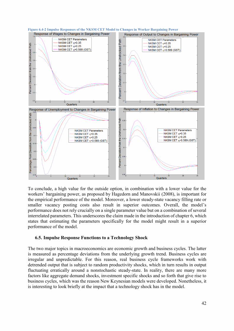
42
Figure 6.4-2 Impulse Responses of the NKSM CET Model to Changes in Worker Bargaining Power
To conclude, a high value for the outside option, in combination with a lower value for the
workers’ bargaining power, as proposed by Hagedorn and Manovskii (2008), is important for
the empirical performance of the model. Moreover, a lower steady-state vacancy filling rate or
smaller vacancy posting costs also result in superior outcomes. Overall, the model’s
performance does not rely crucially on a single parameter value but on a combination of several
interrelated parameters. This underscores the claim made in the introduction of chapter 6, which
states that estimating the parameters specifically for the model might result in a superior
performance of the model.
6.5. Impulse Response Functions to a Technology Shock
The two major topics in macroeconomics are economic growth and business cycles. The latter
is measured as percentage deviations from the underlying growth trend. Business cycles are
irregular and unpredictable. For this reason, real business cycle frameworks work with
detrended output that is subject to random productivity shocks, which in turn results in output
fluctuating erratically around a nonstochastic steady-state. In reality, there are many more
factors like aggregate demand shocks, investment specific shocks and so forth that give rise to
business cycles, which was the reason New Keynesian models were developed. Nonetheless, it
is interesting to look briefly at the impact that a technology shock has in the model.

43
In principle, technology shocks can be incorporated in the NSKM model in at least three ways,
as the literature on neoclassical growth theory distinguishes between three different definitions
of technological progress. Firstly, there is Solow-neutral technological progress, which is also
termed capital augmenting progress. Secondly, there is Harrod-neutral technological progress,
which is also referred to as labor-augmenting technological progress. In the context of
technology shocks, this setup is obtained by combining equation 5.4.2-1 with equation 5.1-2.
Since labor is the only input factor used in the production process, this is the conventional way
a technology shock is implemented in a DMP model.
However, the New Keynesian model developed by CEE is considerably more complex and has
several sectors. The third definition is Hicks-neutral technological progress, which can be
implemented in the intermediate goods sector of the CEE model. This framework is consistent
with the relationship described in equation 6.5-1 if 𝑧𝑡 was assumed to grow over time, rather
than being stationary. The latter, most frequently used case in macroeconomics is called a total
factor productivity (TFP) shock in the literature.43 This thesis implements a TFP shock because
in contrast to a labor augmenting technological shock, hardly any reformulation of the baseline
CEE model is necessary. All that changes is the production function described by equation
5.4.2-1, which now has the form
𝑌𝑗𝑡 = {
𝑧𝑡𝑘𝑗𝑡𝛼 𝑙𝑗𝑡
1−𝛼 − 𝜙, 𝑖𝑓 𝑘𝑗𝑡𝛼 𝑙𝑗𝑡
1−𝛼 ≥ 𝜙
0 , 𝑜𝑡ℎ𝑒𝑟𝑤𝑖𝑠𝑒, 6.5-1
where 𝑧𝑡 denotes the TFP shock denoted by
𝑧𝑡 = 𝑧𝑡−1𝜌
𝑧1−𝜌𝑒𝜖𝑡 , 6.5-2
with 𝜖𝑡~𝑁(0, 𝜎𝜖2).
In neoclassical growth models, only labor-augmenting technological growth is compatible with
the existence of a steady-state. From this perspective, it seems equally realistic to assume that
labor-augmenting technology is subject to random fluctuations. However, given the Cobb-
Douglas production function, the form of technological progress has no effect on the results.
All that changes is the magnitude at which the shock affects total output, because 0 < 𝛼 < 1.
Therefore, the impact of a TFP shock is slightly higher than the impact of an equally sized
labor-augmenting technology shock. However, CEE do not consider technology shocks since
the authors did not seek to evaluate the model along this dimension.44 Gertler et al. (2008)
formulate a labor-augmenting productivity shock in a way that results in technology being
nonstationary in levels, but stationary in growth rates. Furthermore, Christiano et al. (2013)
combine two separate shocks into one composite technology shock.
For the reasons described in the outline of chapter 6, this thesis does not estimate a VAR.
Consequently, no empirical evaluations of the impulse response functions to a technology shock
are available for the model developed here. One way of considering technology shocks is to
assess the differences in the impacts of the NKSM model versus the model developed by CEE.
43 A TFP shock directly affects the efficiency of capital and labor alike and can be seen as anything that changes
the effectiveness of the production process, for given amounts of inputs. Examples are oil price fluctuations,
changes in government regulations, bad weather or innovations due to research and development. 44 The CEE model is specifically tailored to monetary policy shocks. It is unlikely that the model would perform
as well with respect to other dimensions.

44
The following graphs provide IRFs of key macroeconomic variables to a TFP shock. The
parameters of the shock process are provided in Table 6.1-1, with the respective standard
deviations in parenthesis. Parameters for the labor-augmenting technological shock are also
provided but this shock is not implemented into the CEE model and only included for
completeness as well as for potential further research. To facilitate the comparison, the Taylor
rule proposed by CEE is used for all simulated models. All other parameter values are identical
to the ones used before.
Figure 6.5-1 Impulse Response Functions to a TFP Shock in the NKSM CET Model
Figure 6.5-2 Impulse Response Functions to a Neutral Technology Shock in the Cristiano et al. (2013) Model

45
Figure 6.5-1 shows that the response of the benchmark CEE model to a TFP shock is different
to the response of the augmented model. It is impossible to assess the quality of either model
without any empirical estimates for the impulse responses to a TFP shock. Therefore, Figure
6.5-2 provides the impulse responses to a neutral technology shock from Christiano et al.
(2013).
A crude comparison of Figure 6.5-1 with Figure 6.5-2 can assist in determining whether any of
the frameworks produces graphs that are likely to be close to the empirically observed patterns.
However, this is potentially misleading and should be done with caution because the authors
implement the shock in a different way. Given the magnitude at which output, inflation and the
interest rate respond to a positive TFP shock, it seems reasonable to assume that the augmented
model is better able to capture the effect of a TFP shock. According to the VAR estimate, after an
initial increase, output seems to slightly deteriorate for a short period of time before it starts to
surge again.
Both the benchmark CEE model as well as the NKSM model with CET parameterization
establish this behaviour. However, the benchmark model produces a substantially larger rise in
output. As already mentioned in footnote 44, the CEE model is designed to replicate the
observed hump-shaped response of many macroeconomic variables to a monetary policy shock.
Therefore, the authors incorporate frictions that account for this peculiarity.
Figure 6.5-2 shows that the reaction to a TFP shock does not seem to exhibit this kind of
sluggishness in the data. Nonetheless, the CEE model also produces a hump-shaped response
to a TFP shock. As a result, it appears as if the structure of the benchmark CEE model is
insufficient in the case of technology shocks.
To facilitate the comparison, the IRFs of the models as well as the simulated VAR are combined
in one figure. The graphs on the left-hand side of Figure 6.5-3 and Figure 6.5-4 correspond to
the estimates of Christiano et al. (2013). In line with Figure 6.5-2, the dashed green line belongs
to the sticky wage model of the authors, whereas the dotted blue line is the alternating offer
variant. In the NKSM CET parameterization, output as well as unemployment exhibit a fairly
similar pattern as the empirical VAR suggests. However, the response of inflation and the
federal funds rate is too sluggish in this case.
It seems possible that a slightly different parameterization that combines values from the CET
and GST estimates could produce graphs that are fairly close to the VAR impulse responses.
Since the technology shock considered in Christiano et al. (2013) is based on a different setup,
this exercise is omitted here. Overall, it looks as if the NKSM model developed in this thesis is
potentially more capable of replicating the empirically observed pattern of TFP shocks than the
benchmark CEE model. Further research is necessary to answer this question.

46
Figure 6.5-3 Impulse Response of Output, Unemployment and Inflation to a TFP Shock

47
Figure 6.5-4 Impulse Responses of the Interest Rate to a TFP Shock
6.6. Further Research proposals
Despite the fact that the model proposed in this thesis replicates the observed reaction of
important macroeconomic variables like output, investment, consumption and unemployment
reasonably well, there is considerable room for improvement in other key variables. For
instance, the sharp increase in wages, which in turn causes inflation to surge more quickly than
expected, needs to be addressed. In the context of the simple DMP model, wage stickiness
appears to be a good solution, because, empirically, average wages are sticky as well.45
However, what actually matters in the Search and Matching framework is the sluggishness of
wages of newly hired workers, because these wages are relevant for the job creation condition
and thus the hiring choice of firms.46 Pissarides (2009) points out that the DMP model’s
prediction for wages characterizes the behavior of salaries in new jobs quite well. Nonetheless,
the impulse response of inflation is counterfactual to empirical estimates. The model presented
here abstracts from job-to-job transition. It allows only flows from employment to
unemployment, and vice versa. In reality, on-the-job search and job-to-job transition is an
important factor.47
Another popular model extension changes the wage bargaining process. Using alternating offer
bargaining instead of conventional Nash bargaining results in wage negotiations that are
comparatively self-contained.48 As a result, unemployment conditions and wages become less
correlated, which in turn leads to empirically favorable results. Ultimately, this framework also
relies on sluggishness in wages, which derives from the alternating offer bargaining setup rather
than from Calvo-style nominal wage contracts.
45 Shimer (2005) as well as Hall (2005) were the first economists to make this proposal. 46 Haefke et al. (2013) show that wages of newly hired workers are considerably more flexible than wages of the
existing workforce. 47 Van Zanweghe (2009) emphasizes the importance of job-to-job transition. In essence, it mitigates the response
of inflation to an expansionary shock and increases the dissemination towards output. Nonetheless, the author also
uses a sticky wage model 48 Hall and Milgrom (2008) were the first to incorporate the alternating offer framework in a DMP model. The
game theoretical concept was initially solved by Rubinstein (1982).

48
Lubik (2009) illustrates that, in a DMP framework, the principal determinant of labor market
dynamics is an exogenous movement in the matching efficiency. Given this result, the
feasibility of the Search and Matching model as a theory for labor market dynamics becomes
questionable. In general, there exist various labor market models.49 Shimer (2005) proposes an
interesting concept which assumes that it is costly for workers and firms to move between cities
or different types of human capital or markets.50 This framework simultaneously allows for the
existence of unemployment and low wages in one local labor market while job vacancies and
high wages may coexist in another. Overall, there exist numerous competing frameworks that
all deliver promising results. From this perspective, the coming years will be characterized by
a vibrant debate in the literature.
7. Conclusion
This thesis develops and simulates a New Keynesian Dynamic Stochastic General Equilibrium
model that incorporates a variant of the Diamond Mortensen Pissarides Search and Matching
model of the labor market. There are two key research questions. Firstly, are nominal wage
rigidities still an important friction that is essential for the model’s performance? Secondly, is
the augmented framework capable of replicating the empirically observed fluctuations in
involuntary unemployment? The model is calibrated with parameter values from the existing
literature. This thesis simulates the response to an expansionary monetary policy shock as well
as to a TFP shock. However, the focus lies on the former shock, because the New Keynesian
DSGE model that provides the basis for this thesis is tailored to being able to replicate the
impulse responses to monetary policy shocks.
Regarding the expansionary monetary policy shock, the augmented model replicates the
impulse responses of output, unemployment, investment, consumption and the interest rate
quite well. Nonetheless, sticky wages remain crucial in certain parts of the model. For instance,
some form of sluggishness could alleviate the sharp increase in wages, which in turn causes
inflation to surge counterfactually fast. On the other hand, what actually matters in the Search
and Matching framework is the response of wages of newly hired workers, because these wages
are relevant for the job creation condition and thus the hiring choice of firms. Pissarides (2009)
points out that the DMP model’s prediction for wages replicates the behaviour of salaries in
new jobs quite well.
Instead of using generalized Nash bargaining for the determination of wages, researchers have
started to incorporate alternating offer bargaining. As shown in the literature, this framework
results in wage negotiations that are comparatively self-contained. Therefore, unemployment
conditions and wages become less correlated, which in turn leads to empirically favorable
results.
In comparison to conventionally used parameter values, a high value for the outside option, as
proposed by Hagedorn and Manovskii (2008), is important for the empirical performance of
the model. Unlike the Hagedorn and Manovskii suggestion, the model developed in this thesis
does not rely on a low bargaining power value. As explained, this is a result of the substantially
more complex model used in this thesis. Furthermore, the model’s ability to replicate the
49 Rogerson et al. (2005) provide an excellent survey of search-theoretic models of the labor market. Shimer (2008)
discusses the benefits and shortcomings of various labor market theories. 50 Shimer’s paper is essentially an extension of work on the matching processes between taxicabs and riders within
cities, developed by Lagos (2000).

49
observed impulse response functions is supported by a lower steady-state vacancy filling rate
or smaller vacancy posting costs. Overall, the model’s performance does not rely decisively on
a single parameter value. On the contrary, a combination of several interrelated parameters
appears to explain the superior performance of the parameterization according to Christiano et
al. (2013).
Generally, it looks as if the NKSM model developed in this thesis is potentially more capable
of replicating the empirically observed pattern of TFP shocks than the benchmark CEE model.
Nonetheless, further research is needed to answer this question.

50
A. Appendix
The appendix includes the derivations for all the important equations as well as the exact steps
in the log-linearization of these equations. Parts of the New Keynesian model that are not
derived in the appendix can be found in the working paper of Christiano et al. (2001). Moreover,
all Dynare and MATLAB files needed to replicate the simulations and graphs of this thesis are
listed as well.
A.1. Real Marginal Cost of a Cobb-Douglas Production Technology
The following section derives the real marginal cost equation from section 3.5. The cost
minimization problem in real terms has the form
𝑚𝑖𝑛 𝑟𝑡𝑘, 𝑤𝑡
= 𝑟𝑡𝑘𝑘𝑗𝑡 + 𝑤𝑡𝑅𝑡𝑙𝑗𝑡,
subject to 𝑌𝑗𝑡 = 𝑘𝑗𝑡𝛼 𝑙𝑗𝑡
1−𝛼, as defined in equation 6.5-1. Note that 𝑌𝑗𝑡 is an arbitrary level of output,
which is assumed to be equal to unity for simplicity. Therefore, the Lagrange has the form
ℒ = 𝑟𝑘𝑘 + 𝑤𝑅𝑙 − 𝜆(𝑘𝛼𝑙1−𝛼 − 1),
where the minimization problem was reformulated into a maximization problem and all
subscripts were omitted for convenience. This is feasible because each firm in the intermediate
goods sector faces the same cost minimization problem in each period. The corresponding
FOCs are:
𝜕ℒ
𝜕𝑘: 𝑟𝑘 − 𝜆𝛼𝑘𝛼−1𝑙1−𝛼 = 0 A1.i
𝜕ℒ
𝜕𝑙: 𝑤𝑅 − 𝜆(1 − 𝛼)𝑘𝛼𝑙−𝛼 = 0 A1.ii
𝜕ℒ
𝜕𝜆: 𝑘𝛼𝑙1−𝛼 − 1 = 0 A1.iii
Dividing equation A1.i by equation A1.ii yields
𝑟𝑘
𝑤𝑅=
𝛼𝑙
(1 − 𝛼)𝑘,
which can be solved for
𝑙 =
𝑟𝑘(1 − 𝛼)𝑘
𝑤𝑅𝛼. A1.iv
Substituting this into equation A1.iii gives after some rearrangement
𝑘 = (
𝑟𝑘(1 − 𝛼)
𝛼𝑤𝑅)
𝛼−1
, A1.v

51
which, after being plugged into equation A1.iv, solves for
𝑙 = (
𝑟𝑘(1 − 𝛼)
𝛼𝑤𝑅)
𝛼
. A1.vi
Equations A1.v and A1.vi are the regular conditional input factor demand functions that arise
in cost minimization with a Cobb-Douglas production function. As outlined in section 3.5, total
period 𝑡 real costs for an intermediate goods firm are 𝑠𝑡(𝑌𝑡, 𝑟𝑡𝑘, 𝑤𝑡𝑅𝑡) = 𝑟𝑡
𝑘𝑘 + 𝑤𝑡𝑙𝑗𝑡𝑅𝑡.
Using the conditional input factor demand functions, the cost function can be simplified to
equation 3.5-2 via the following steps. In line with above, subscripts are dropped for simplicity.
𝑠 = 𝑟𝑘 (𝑟𝑘(1 − 𝛼)
𝛼𝑤𝑅)
𝛼−1
+ 𝑤𝑅 (𝑟𝑘(1 − 𝛼)
𝛼𝑤𝑅)
𝛼
= 𝑟𝑘(𝑟𝑘)𝛼−1(𝑤𝑅)−(𝛼−1) ((1 − 𝛼)
𝛼)
𝛼−1
+𝑤𝑅(𝑤𝑅)−𝛼(𝑟𝑘)𝛼 ((1 − 𝛼)
𝛼)
𝛼
= (𝑟𝑘)𝛼(𝑤𝑅)1−𝛼 ((1 − 𝛼)
𝛼)
𝛼−1
+ (𝑤𝑅)1−𝛼(𝑟𝑘)𝛼 ((1 − 𝛼)
𝛼)
𝛼
= (𝑟𝑘)𝛼(𝑤𝑅)1−𝛼 (((1 − 𝛼)
𝛼)
𝛼−1
+ ((1 − 𝛼)
𝛼)
𝛼
)
= (𝑟𝑘)𝛼(𝑤𝑅)1−𝛼 (𝛼1−𝛼
(1 − 𝛼)1−𝛼+(1 − 𝛼)𝛼
𝛼𝛼)
= (𝑟𝑘)𝛼(𝑤𝑅)1−𝛼 (𝛼1−𝛼𝛼𝛼
(1 − 𝛼)1−𝛼𝛼𝛼+(1 − 𝛼)𝛼(1 − 𝛼)1−𝛼
𝛼𝛼(1 − 𝛼)1−𝛼)
= (𝑟𝑘)𝛼(𝑤𝑅)1−𝛼 (𝛼
(1 − 𝛼)1−𝛼𝛼𝛼+
1 − 𝛼
𝛼𝛼(1 − 𝛼)1−𝛼)
= (𝑟𝑘)𝛼(𝑤𝑅)1−𝛼 (1
(1 − 𝛼)1−𝛼𝛼𝛼).
The last expression, after reinserting the subscripts, can be rewritten to the final form
𝑠𝑡 = (1
1 − α)1−𝛼
(1
𝛼)𝛼
(𝑟𝑡𝑘)
𝛼(𝑤𝑡𝑅𝑡)
1−𝛼,
which is identical to the equation 3.5-2.

52
A.2. Log-Linearization
With few exceptions, no closed form solutions exist for non-linear difference equations that
arise in discrete time dynamic economic problems. Consequently, approximation techniques
are used with numerical methods to solve these problems. The simulations are obtained with
the Dynare software package (Adjemian, et al., 2011), that is run on top of MATLAB. However,
log-linearization of the non-linear difference equations is done manually.
Linearization is useful because it significantly mitigates the computational workload and
facilitates solving models that may otherwise be intractable. Taking the natural logarithm prior
to linearization results in an equation that is linear in terms of the log-deviations of the
corresponding variables from their steady-state values. If these deviations are sufficiently small,
they approximate the percentage deviation from a steady-state, which provides a convenient
economic interpretation.
Formally, the grapheme “tilde” over a variable is used to indicate the percentage deviation from
its steady-state value, defined as
��𝑡 =
𝑤𝑡 −𝑊
𝑊≈ 𝑙𝑜𝑔(𝑤𝑡) − log (𝑊), A2.i
where a variable without a hat or subscript symbolizes its non-stochastic steady-state value.51
As usual, capital letters denote nominal variables, whereas lower case letters correspond to real
variables. At the risk of creating possible confusion, notation is simplified throughout the text
and the Dynare code by also using capital letters for the steady-state of a variable. Nonetheless,
these two can be distinguished because nominal variables include a time subscript.
For example, the Cobb-Douglas production function of equation 6.5-1, 𝑦𝑗𝑡 = 𝑧𝑡𝑘𝑗𝑡𝛼 𝑙𝑗𝑡
1−𝛼, can be
rewritten in logarithmic form as
ln(𝑦𝑡) = ln(zt) + α ln(kt) + (1 − α) ln(lt),
which was simplified by using the basic properties of the natural logarithm and dropping the
firm specific subscript. Note that until now, no approximation took place. Linearization is
achieved with a first-order Taylor expansion.
Therefore,
ln(𝑌) +1
𝑌(𝑦𝑡 − 𝑌)
= ln(𝑍) +1
𝑍(𝑧𝑡 − 𝑍) + 𝛼 ln(𝐾) +
𝛼
𝐾(𝑘𝑡 − 𝐾) + (1 − 𝛼) ln(𝐿)
+1 − 𝛼
𝐿(𝑙𝑡 − 𝑙).
51 Note that CEE indicate the percentage deviation from the steady-state value with a “hat” rather than a “tilde”
over a variable.

53
Using the fact that ln(𝑌) = ln(𝑍) + 𝛼 ln(𝐾) + (1 − 𝛼)ln (𝐿), these terms cancel and the
equation above can be simplified to
��𝑡 = ��𝑡 + 𝛼��𝑡 + (1 − 𝛼)𝑙𝑡,
where the definition for the percentage deviation from the steady-state value of equation A2.i
was used.
However, there are more ways log-linearization can be achieved. Another convenient approach
computes a first order Taylor expansion of some arbitrary multivariate function 𝑓(𝑥𝑡, 𝑦𝑡) around the steady-state value directly as
𝑓(𝑥𝑡, 𝑦𝑡) ≈ 𝑓(𝑋, 𝑌) +𝜕𝑓(𝑋, 𝑌)
𝜕𝑥𝑋��𝑡 +
𝜕𝑓(𝑋, 𝑌)
𝜕𝑦𝑌��𝑡.
Take the generic resource constraint 𝑦𝑡 = 𝑖𝑡 + 𝑐𝑡 as a simple example. Applying the technique
described above yields
𝑌 + 𝑌𝑦𝑡 − 𝑌
𝑌= 𝐼 + 𝐶 + 𝐼
𝑖𝑡 − 𝐼
𝐼+ 𝐶��𝑡.
The steady-state terms, 𝑌 = 𝐼 + 𝐶, cancel and the equation becomes
𝑌��𝑡 = 𝐼𝑖𝑡 + 𝐶��𝑡.
Another frequently used representation of the same resource constraint is achieved by dividing
the equation above by 𝑌. Therefore,
��𝑡 =𝐼
𝑌𝑖𝑡 +
𝐶
𝑌��𝑡.
To prove that both procedures provide the same result, the logarithmic form of the resource
constraint is
ln(𝑦𝑡) = ln(𝑖𝑡 + 𝑐𝑡).
Linearization with a first-order Taylor expansion yields
ln(𝑌) +1
𝑌(𝑦𝑡 − 𝑌) = ln(𝐼 + 𝐶) +
1
𝐼 + 𝐶(𝑖𝑡 − 𝐼) +
1
𝐼 + 𝐶(𝑐𝑡 −).
Again, ln (𝑌) = ln (𝐼 + 𝐶) cancels and the equation above can be simplified to
��𝑡 =𝐼
𝑌𝑖𝑡 +
𝐶
𝑌��𝑡.
which is identical to the result above.

54
A.3. The Log-Linearized System of the CEE Model
All equations that are relevant for simulating the model developed in this thesis are log-
linearized with one of the two methods outlined in section A.2 of the appendix. Christiano et
al. (2001) use thirteen Euler and other equations to solve the dynamics of the system. Moreover,
the Dynare code uses seven auxiliary equations that facilitate finding the solution. The
following subsections describe all these equations. For the sake of brevity, only the more
complex derivations are shown in detail for the CEE model. The numeric listing is identical to
the Dynare code provided in section A.4.
A.3.1. The Inflation Phillips Curve
To facilitate a coherent characterization of the intermediate goods sector problem, the inflation
Phillips curve was already discussed in section 3.5. Therefore, no further details will be given
here. For ease of reference, equation 3.5-10 is quoted again:
��𝑡 =
1
1 + 𝛽��𝑡−1 +
𝛽
1 + 𝛽𝐸𝑡��𝑡+1 +
(1 − 𝛽𝜉𝑝)(1 − 𝜉𝑝)
𝜉𝑝𝐸𝑡��𝑡 A.3.1
A.3.2. The Money Demand Function
Equation 3.6-9 describes the household’s FOC for nominal cash balances. Log-linearization
yields, after dropping constant terms and solving for cash balances:
��𝑡 = −
1
𝜎𝑞[
𝑅
𝑅 − 1��𝑡 + ��𝑐,𝑡 ] A.3.2
A.3.3. The “Wage Phillips Curve”
The equation involving the aggregate wage rate is derived as the log-linearized equation 3.7-5,
together with 3.7-2. For ease of reference, these equations are quoted again:
Ε𝑡∑(𝛽𝜉𝑤)𝑙𝜓𝑐,𝑡+𝑙 (
��𝑡𝑋𝑡𝑙𝑃𝑡+𝑙
− 𝜆𝑤2𝜓0(𝑛𝑖,𝑡+𝑙)
𝜓𝑐,𝑡+𝑙)𝑛𝑖,𝑡+𝑙 = 0
∞
𝑙=0
,
𝑛𝑖𝑡 = (𝑊𝑡
𝑊𝑖𝑡)
𝜆𝑤𝜆𝑤−1
𝑙𝑡.
CEE use a few additional definitions in their working paper:
��𝑡 =
𝑄𝑡𝑃𝑡−1
, ��𝑡 =𝑊𝑡
𝑃𝑡−1 , ��𝑡 =
��𝑡
𝑊𝑡. A.3.3.i
In percentage terms, the deviation of the household’s real wage rate from its non-stochastic
steady-state value is given by ��𝑡 + ��𝑡. Moreover, ��𝑡 = ��𝑡 − ��𝑡, where 𝜋𝑡 corresponds to the
time 𝑡 inflation rate, denoted by 𝜋𝑡 = 𝑃𝑡/𝑃𝑡−1. This result follows from taking logs of the term
in the middle of the equation A.3.3.i, which yields

55
ln(��𝑡) = ln(𝑊𝑡) − ln(𝑃𝑡−1).
The term ln(𝑊𝑡) can be rewritten using the definition of real variables, 𝑤𝑡 = 𝑊𝑡/𝑃𝑡. Therefore,
ln(��𝑡) = ln(𝑤𝑡) − ln (𝑃𝑡) − ln(𝑃𝑡−1).
The time 𝑡 inflation rate in log-linearized terms has the form ��𝑡 = ��𝑡 − ��𝑡−1. Consequently,
��𝑡 = ��𝑡 − ��𝑡. A.3.3.ii
Log-linearization of equation 3.7-5, using equation 3.7-2 results in
��𝑡 + ��𝑡 =∑(𝛽𝜉𝑤)
𝑙
∞
𝑙=1
(��𝑡+𝑙 − ��𝑡+𝑙−1)
+(1 − 𝛽𝜉𝑤)(𝜆𝑤 − 1)
2𝜆𝑤 − 1∑(𝛽𝜉𝑤)
𝑗
∞
𝑗=𝑙
[�� 𝑡+𝑗 +𝜆𝑤
𝜆𝑤 − 1��𝑡+𝑗 − ��𝑐,𝑡+𝑗].
A.3.3.iii
Comparable to equation 3.5-7, equation 3.7-3 can be rewritten as
𝑊𝑡 = [(1 − 𝜉𝑤)��𝑡
11−𝜆𝑤 + 𝜉𝑤(𝜋𝑡−1𝑤𝑡−1)
11−𝜆𝑤]
1−𝜆𝑤
.
Dividing this equation by the price level of the current period, and log-linearizing, yields
(1 − 𝜉𝑤)��𝑡 = 𝜉𝑤��𝑡 − 𝜉𝑤(��𝑡−1(��𝑡 − ��𝑡−1)). A.3.3.iv
Merging equation A.3.3.iii with A.3.3.iv results, after some rearrangement, in the final equation
��𝑡−1 =
𝑏𝑤(1 + 𝛽𝜉𝑤2 ) − 𝜆𝑤
𝑏𝑤𝜉𝑤𝐸𝑡��𝑡 − 𝛽𝐸𝑡��𝑡+1
− 𝐸𝑡[𝛽(��𝑡+1 − ��𝑡) − (��𝑡 − ��𝑡−1)]
−1 − 𝜆𝑤𝑏𝑤𝜉𝑤
𝐸𝑡(��𝑐,𝑡 − 𝑙𝑡),
A.3.3
where 𝑏𝑤 =2𝜆𝑤−1
(1−𝜉𝑤)(1−𝛽𝜉𝑤).
A.3.4. The Household‘s Intertemporal Euler Equation
Equation 3.6-10 corresponds to the FOC with respect to the household’s beginning of
period 𝑡 + 1 money stock, which has the log-linearized form
𝐸𝑡(��𝑐,𝑡+1 + ��𝑡+1 − ��𝑡+1 − ��𝑐,𝑡) = 0 A.3.4
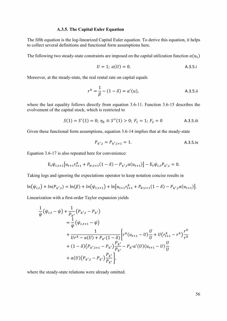
56
A.3.5. The Capital Euler Equation
The fifth equation is the log-linearized Capital Euler equation. To derive this equation, it helps
to collect several definitions and functional form assumptions here.
The following two steady-state constraints are imposed on the capital utilization function 𝑎(𝑢𝑡)
𝑈 = 1; 𝑎(𝑈) = 0. A.3.5.i
Moreover, at the steady-state, the real rental rate on capital equals
𝑟𝑘 =
1
𝛽− (1 − 𝛿) = 𝑎′(𝑢), A.3.5.ii
where the last equality follows directly from equation 3.6-11. Function 3.6-15 describes the
evolvement of the capital stock, which is restricted to
𝑆(1) = 𝑆′(1) = 0; 𝜂𝑘 ≡ 𝑆′′(1) > 0; 𝐹1 = 1; 𝐹2 = 0 A.3.5.iii
Given these functional form assumptions, equation 3.6-14 implies that at the steady-state
𝑃𝑘′,𝑡 = 𝑃𝑘′,𝑡+1 = 1. A.3.5.iv
Equation 3.6-17 is also repeated here for convenience:
Ε𝑡𝜓𝑐,𝑡+1[𝑢𝑡+1𝑟𝑡+1𝑘 + 𝑃𝑘′,𝑡+1(1 − 𝛿) − 𝑃𝑘′,𝑡𝑎(𝑢𝑡+1)] − Ε𝑡𝜓𝑐,𝑡𝑃𝑘′,𝑡 = 0.
Taking logs and ignoring the expectations operator to keep notation concise results in
ln(𝜓𝑐,𝑡) + 𝑙𝑛(𝑃𝑘′,𝑡) = ln(𝛽) + 𝑙𝑛(𝜓𝑐,𝑡+1) + ln [𝑢𝑡+1𝑟𝑡+1𝑘 + 𝑃𝑘′,𝑡+1(1 − 𝛿) − 𝑃𝑘′,𝑡𝑎(𝑢𝑡+1)].
Linearization with a first-order Taylor expansion yields
1
𝜓(𝜓𝑐,𝑡 − 𝜓) +
1
𝑃𝑘′(𝑃𝑘′,𝑡 − 𝑃𝑘′)
=1
𝜓(𝜓𝑐,𝑡+1 − 𝜓)
+1
𝑈𝑟𝑘 − 𝑎(𝑈) + 𝑃𝑘′(1 − 𝛿)[𝑟𝑘(𝑢𝑡+1 − 𝑈)
𝑈
𝑈+ 𝑈(𝑟𝑡+1
𝑘 − 𝑟𝑘)𝑟𝑘
𝑟𝑘
+ (1 − 𝛿)(𝑃𝑘′,𝑡+1 − 𝑃𝑘′)𝑃𝑘′
𝑃𝑘′− 𝑃𝑘′𝑎
′(𝑈)(𝑢𝑡+1 − 𝑈)𝑈
𝑈
+ 𝑎(𝑈)(𝑃𝑘′,𝑡 − 𝑃𝑘′)𝑃𝑘′
𝑃𝑘′ ],
where the steady-state relations were already omitted.

57
This can be greatly simplified using equations A.3.5.i to A.3.5.iv. The term preceding the square
brackets can be reformulated with the following steps:
1
𝑈𝑟𝑘 − 𝑎(𝑈) + 𝑃𝑘′(1 − 𝛿)=
1
𝑟𝑘 + (1 − 𝛿)=
1
1𝛽− (1 − 𝛿) + (1 − 𝛿)
= 𝛽. A.3.5.v
Consequently, the total equation can be written as
��𝑐,𝑡 + ��𝑘′,𝑡 = ��𝑐,𝑡+1
+ 𝛽[𝑟𝑘𝑈��𝑡+1 + 𝑈𝑟𝑘��𝑡+1𝑘 + (1 − 𝛿)𝑃𝑘′��𝑘′,𝑡+1 − 𝑃𝑘′𝑎
′(𝑈)𝑈��𝑡+1+ 𝑎(𝑈)𝑃𝑘′��𝑘′,𝑡].
Moreover, the term in square brackets can be simplified further. Since 𝑃𝑘′ = 1, the first and
fourth term cancel each other due to A.3.5.ii. The fifth drops out because of A.3.5.i. Thus,
��𝑐,𝑡 + ��𝑘′,𝑡 = ��𝑐,𝑡+1 + 𝛽[𝑟𝑘��𝑡+1𝑘 + (1 − 𝛿)��𝑘′,𝑡+1].
Applying similar steps as the ones carried out in equation A.3.5.v, this expression can be written
as
��𝑐,𝑡 + ��𝑘′,𝑡 = ��𝑐,𝑡+1 + [1 − 𝛽(1 − 𝛿)]��𝑡+1𝑘 + (1 − 𝛿)𝛽��𝑘′,𝑡+1.
Substituting for the return on capital, given by ��𝑡+1𝑘 = ��𝑡+1 + ��𝑡+1 + 𝑙𝑡+1 − ��𝑡+1, results in the
final solution, which after reinserting the expectations operator is identical to the equation
provided by CEE
0 = 𝐸𝑡{−��𝑘′,𝑡 − ��𝑐,𝑡 + ��𝑐,𝑡+1 + (1 − 𝛽(1 − 𝛿))[��𝑡+1 + ��𝑡+1 + 𝑙𝑡+1 − ��𝑡+1]
+ 𝛽(1 − 𝛿)��𝑘′,𝑡+1}. A.3.5
A.3.6. The Aggregate Resource Constraint
For convenience, the derivation is postponed to subsection A.4.1. This is useful because the
steps are identical except for an additional term that accounts for vacancy posting costs in the
augmented model. The log-linearized form of the resource constraint provided in equation 3.9-2
is given by
[1
𝛽− (1 − 𝛿)]
𝑠𝐾𝑠𝑐��𝑡 + ��𝑡 +
𝛿𝑠𝑘𝑠𝑐
𝑖𝑡 =𝛼
𝑠𝑐��𝑡 +
1 − 𝛼
𝑠𝑐��𝑡. A.3.6
A.3.7. The Loan Market Clearing Condition
Equation 3.9-1 in real terms has the form 𝜇𝑡𝑚𝑡 − 𝑞𝑡 = 𝑤𝑡𝑙𝑡. Log-linearization results in
��𝑡 + 𝑙𝑡 =1
𝜇𝑀 − 𝑄(𝑀(𝜇𝑡 − 𝜇)
𝜇
𝜇+ 𝜇(𝑚𝑡 −𝑀)
𝑀
𝑀− (𝑞𝑡 − 𝑄)
𝑄
𝑄).
At the steady-state, 𝑤𝐿 = 𝜇𝑀 − 𝑄.

58
Therefore, combining terms and rearranging yields
𝜇𝑀(𝜇𝑡 + ��𝑡) − 𝑄��𝑡 − 𝑤𝐿(��𝑡 + 𝑙𝑡) = 0. A.3.7
A.3.8. The Money Growth Rate
The money growth rate is defined as 𝜇𝑡−1 =𝑀𝑡
𝑀𝑡−1. Log-linearization gives
𝜇𝑡−1 + ��𝑡−1 − ��𝑡 − ��𝑡 = 0, A.3.8
where again, prior to log-linearization, the definition of real variables, 𝑤𝑡 = 𝑊𝑡/𝑃𝑡, was used
to rewrite the equation as
𝜇𝑡−1 =𝑚𝑡𝑃𝑡
𝑚𝑡−1𝑃𝑡−1.
A.3.9. The Generalized Habit Formation
CEE define the utility of consumption as 𝑐𝑡 − 𝐻𝑡, with 𝐻𝑡 = 𝜒𝐻𝑡−1 + 𝑏𝑐𝑡−1.52 Log-
linearization yields
��𝑡 =1
𝜒𝐻+𝑏𝐶(𝜒(𝐻𝑡−1 − 𝐻) + 𝑏(𝑐𝑡−1 − 𝑐)
𝐶
𝐶),
where the steady-state relations 1
𝜒𝐻+𝑏𝐶= 𝐻 and 𝐻(1 − 𝜒) = 𝑏𝑐 can be used to rewrite it as
��𝑡 − 𝜒��𝑡−1 − (1 − 𝜒)��𝑡−1 = 0. A.3.9
However, CEE estimate a value of 𝜒 = 0, which essentially renders this equation futile.
Equation A.3.9 is only kept in the system of equations to keep notation in line with CEE.
A.3.10. The Generalized Consumption Euler Equation
Equation 3.6-7, together with equations 3.6-8 and A.3.9 can be log-linearized to the form
𝐸𝑡
{
−𝛽𝜒��𝑐,𝑡+1 + ��𝑐𝑖 [��𝑡 −
𝑏
1 − 𝜒��𝑡]
−(𝑏 + 𝜒)𝛽��𝑐𝑖 [��𝑡+1 −
𝑏
1 − 𝜒𝐻𝑡+1] + ��𝑐,𝑡}
= 0, A.3.10
with ��𝑐𝑖 =
1−𝜒
1−𝜒−𝑏
1−𝛽𝜒
1−𝛽𝜒−𝛽𝑏 .53
52 Note that the working paper of CEE erroneously writes 𝐻𝑡 = 𝜓𝐻𝑡−1 + 𝑏𝑐𝑡−1. 53 Note that given 𝜒 = 0, equation A.3.A.3.10 collapses to the standard version because ��𝑡 = (1 − 𝜒)��𝑡−1.
Therefore, ��𝑡 − 𝑏/(1 − 𝜒)𝐻𝑡 becomes ��𝑡 − 𝑏��𝑡−1.

59
A.3.11. The Investment Euler Equation
The log-linearized form of 3.6-14 is
𝐸𝑡��𝑘′,𝑡 = 𝜂𝑘𝐸𝑡{𝑖𝑡 − 𝑖𝑡−1 − 𝛽[𝑖𝑡+1 − 𝑖𝑡]}, A.3.11
where equations A.3.5.iii and A.3.5.iv were used for the derivation.
A.3.12. The Capital Accumulation Equation
Capital evolves according to equation 3.6-3, which using the equation 3.6-15, together with the
corresponding functional form assumptions provided in A.3.5.iii yields the log-linearized form
��𝑡+1 = (1 − 𝛿)��𝑡 + 𝛿𝑖𝑡, A.3.12
where the steady-state relation 𝑖 = 𝛿𝑘 was used.
A.3.13. The Household’s Capital Utilization Decision
The Euler equation linked to the household’s capital utilization decision is given by equation
3.6-11. Using the functional form assumptions of equation A.3.5.i and the inverse of the
elasticity of the utilization rate to the rental rate of capital as defined in equation 6.3-1, the log-
linearized form becomes
𝐸𝑡[��𝑡𝑘 − 𝜎𝑎��𝑡] = 0 A.3.13
This completes the derivation of the thirteen equations used by CEE. The following seven
auxiliary equations augment the system in a way that facilitates the solution process in Dynare.
A.3.14. The Definition of Capacity Utilization
Recall from section 3.6 that the physical capital stock, ��𝑡, is associated with capital services via
the relationship 𝑘𝑡 = 𝑢𝑡��𝑡, with 𝑢𝑡 symbolizing the utilization rate of capital. Log- linearization
results in
��𝑡 = ��𝑡 − ��𝑡, A.3.14
where the Dynare code takes into account that the physical capital stock is assumed to be
predetermined in the system.
A.3.15. The Return on Capital
As already mentioned in the discussion of equation A.3.5, the return on capital has the following
log-linearized form
��𝑡+1𝑘 = ��𝑡+1 + ��𝑡+1 + 𝑙𝑡+1 − ��𝑡+1. A.3.15

60
A.3.16. The Taylor Rule
Using the properties of the natural logarithm, the Taylor rule described in equation 6.2-1 can
be expressed as
ln(𝑅𝑡) − ln(𝑅)= 𝜌𝑟[ln(𝑅𝑡−1) − ln(𝑅)]+ (1 − 𝜌𝑟)[𝜌𝜋(ln(𝜋𝑡) − ln(𝜋)) + 𝜌𝑌 (ln(𝑌𝑡) − ln(𝑌))] + 𝜖𝑡.
A first order Taylor expansion around steady-state yields, after dropping constant terms, the
form
��𝑡 = 𝜌𝑟��𝑡−1 + (1 − 𝜌𝑟)[𝜌𝜋��𝑡 + 𝜌𝑌Yt] + 𝜖𝑡. 0.a
Consequently, the CEE variant described in section 3.8 has the log-linearized form
��𝑡 = 𝜌𝑟��𝑡−1 + (1 − 𝜌𝑟)[𝜌𝜋Ε𝑡��𝑡+1 + 𝜌𝑌Yt] + 𝜖𝑡. 0.b
A.3.17. Real Marginal Cost
As derived in appendix A.1, cost minimization in the intermediate goods sector implies that
real marginal costs have the form of equation 3.5-2. Log-linearization yields
��𝑡 = 𝛼��𝑡𝑘 + (1 − 𝛼)��𝑡��𝑡. A.3.17
A.3.18. The Cobb-Douglas Production Function
Equation 5.4.2-1 describes the production function in the intermediate goods sector, which has
the following log-linearized form:
��𝑡 = 𝛼��𝑡 + (1 − 𝛼)𝑙𝑡. A.3.18
A.3.19. The Real Wage as Defined in CEE
CEE define the wage in their thirteen variable system as shown in equation A.3.3.i. For ease of
reference, the corresponding log-linearized form, equation A.3.3.ii, is quoted again:
��𝑡 = ��𝑡 − ��𝑡. A.3.19
A.3.20. Real Cash Balances
Consistent with equation A.3.19, real cash balances in log-linearized form give
��𝑡 = ��𝑡 − ��𝑡. A.3.20
A.4. The Log-Linearized System of the DMP Model
The following subsections list the system of log-linearized equations of the incorporated DMP
model, as described in chapter 5.

61
A.4.1. The Aggregate Resource Constraint
In addition to the standard resource constraint used in CEE, vacancy posting costs need to be
taken into account. Moreover, the Search and Matching framework now determines the
aggregate amount of the homogeneous labor input used in the intermediate production process.
A few considerations are needed to derive the final equation. As explained in section 3.5, capital
and labor is rented in perfectly competitive factor markets. Consequently, each producer faces
identical factor prices and constant returns to scale in the production function imply that there
is no need to distinguish between firms. Thus, the unweighted average of output can be
expressed as
𝑌∗ = ∫ 𝑌𝑗𝑑𝑗 = ∫ 𝑘𝑗
𝛼𝑙𝑗1−𝛼𝑑𝑗 = 𝑘𝛼𝑙1−𝛼,
1
0
1
0
A.4.1.i
where 𝑘 and 𝑙 represent the aggregate amount of capital and of the homogenous labor input:54
𝑘 = ∫ 𝑘𝑗𝑑𝑗
1
0
; 𝑙 = ∫ 𝑙𝑗𝑑𝑗.1
0
A.4.1.ii
Time subscripts are omitted in order to be consistent with the derivation provided in the working
paper of Christiano et al. (2001). Eventually, time subscripts will be reinserted to provide a
correct representation of the log-linearized resource constraint. The authors list two reasons
why this is not the best way to express the aggregate resource constraint. Firstly, total output
should be related to total labor, calculated as in equation 5.5-1. This is preferable because 𝑛𝑡 characterizes labor as measured in the data, whereas 𝑙𝑡 is the amount of the homogenous labor
input used in the intermediate goods production. Secondly, 𝑌∗ does not have any meaningful
economic interpretation, because it is simply a sum of differentiated intermediate goods. The
latter problem can be solved by substituting optimal demand for intermediate good 𝑗, characterized by equation 3.4-2, into A.4.1.i:
𝑌∗ = ∫ 𝑌𝑗𝑑𝑗 = ∫ (𝑃
𝑃𝑗)
𝜆𝑓𝜆𝑓−1
𝑌𝑑𝑗 = 𝑌𝑃
𝜆𝑓𝜆𝑓−1(𝑃∗)
𝜆𝑓1−𝜆𝑓 ,
1
0
1
0
where 𝑃∗ denotes the weighted average of all individual prices.55 Solving for 𝑌 and substituting
out 𝑌∗ with the last term in equation A.4.1.i. gives
𝑌 = (𝑃∗
𝑃)
𝜆𝑓𝜆𝑓−1
𝑘𝛼𝑙1−𝛼.
Instead of the unweighted average output, this equation now contains the aggregate output,
which is allocated between consumption, investment, the resources used up in capital utilization
54 CEE use capital letters, whereas here lower case letters are used to avoid confusion with steady-state values.
55 Note that the weights are not identical to the ones used in equation 3.4-3 because 𝑃∗ = [∫ 𝑃𝑗
𝜆𝑓
1−𝜆𝑓1
0𝑑𝑗]
1−𝜆𝑓
𝜆𝑓
.

62
as well as the total vacancy posting costs. Consequently, the model economy is facing the
following modified resource constraint:
𝑐 + 𝑖 + 𝑎(𝑢)�� + 𝜅𝑣 ≤ (𝑃∗
𝑃)
𝜆𝑓𝜆𝑓−1
𝑘𝛼𝑙1−𝛼.
The last modification needed regards the total labor force. Substituting equation 5.1-2, using
definitions 5.5-1 and A.4.1.ii, gives
𝑐 + 𝑖 + 𝑎(𝑢)�� + 𝜅𝑣 ≤ (𝑃∗
𝑃)
𝜆𝑓𝜆𝑓−1
𝑘𝛼(𝐴𝑛)1−𝛼, A.4.1.iii
which corresponds to the sought-after resource constraint of equation 5.5-2. CEE state that the
term in front of the production function is similar to the so called Solow residual, which is
essentially the TFP part, denoted as 𝑧𝑡, of the production function described in equation 6.5-1.
Yun (1996) showed that in a first order approximation, as used here, this “Solow residual” is a
constant. As CEE highlight, this result can be found by obtaining expressions for 𝑊∗/𝑊 and
𝑃∗/𝑃 respectively.
Equivalent to the way equation 3.4-3 was rewritten in the form of equation 3.5-7, 𝑃𝑡∗
and , 𝑊𝑡∗can be expressed as
𝑃𝑡∗ = [(1 − 𝜉𝑝)��𝑡
𝜆𝑓
1−𝜆𝑓 + 𝜉𝑝(𝜋𝑡−1𝑃𝑡−1∗ )
𝜆𝑓1−𝜆𝑓]
1−𝜆𝑓𝜆𝑓
.
Dividing this term by 𝑃𝑡 yields
𝑝𝑡∗ = [(1 − 𝜉𝑝)��𝑡
𝜆𝑓
1−𝜆𝑓 + 𝜉𝑝(𝜋𝑡−1𝑝𝑡−1∗ )
𝜆𝑓1−𝜆𝑓]
1−𝜆𝑓𝜆𝑓
, A.4.1.iv
where 𝑝∗ = 𝑃∗/𝑃𝑡. Log-linearizing this expression around the steady-state results in
𝑝𝑡∗ = (1 − 𝜉𝑝)��𝑡 + 𝜉𝑝(��𝑡−1 − ��𝑡 + 𝑝𝑡−1
∗ ).
After substituting equation 3.5-8 into the log-linearized expression one obtains
𝑝𝑡∗ = 𝜉𝑝��𝑡−1
∗ .
Let’s supddpose 𝑝0∗ = 0. Therefore, 𝑝𝑡
∗ = 0 for all future time periods and consequently, 𝑃𝑡∗ =
𝑃𝑡 for all possible realizations of t. Since the almost identical steps apply for 𝑊𝑡∗ and this part
is not required in the augmented model, this derivation is left out here.56 During log-
linearization, the transformations above can be used to rationalize considering 𝑃∗/𝑃 as constant
56 CEE provide this part in their working paper appendix (2001).

63
equal to unity. For this reason, the following steps obtain the log-linearized resource constraint
of equation A.4.1.iii. Using the properties of the natural logarithm, this constraint can be written
as
ln(𝑎(𝑢)�� + 𝑐 + 𝑖 + 𝜅𝑣) =𝜆𝑓
𝜆𝑓 − 1ln (
𝑃∗
𝑃) + (1 − 𝛼) ln(𝐴) + (1 − 𝛼) ln(𝑛) + 𝛼 ln(𝑘),
where the inequality sign was switched to an equality sign because at the optimum all output is
used up. After reinserting the omitted time subscripts, a linear first order Taylor expansion
yields,
ln(𝑎(𝑈)�� + 𝐶 + 𝐼 + 𝜅𝑉) +1
𝑌(𝑎′(𝑢)��𝑈��𝑡 + 𝑎(𝑈)����𝑡 + 𝑐��𝑡 + 𝑖𝑖𝑡 + 𝜅𝑉��𝑡)
= (1 − 𝛼) ln(𝐴) + (1 − 𝛼)��𝑡 + (1 − 𝛼) ln(𝑁) + (1 − 𝛼)��𝑡 + 𝛼 ln(𝐾) + 𝛼��𝑡
Using the relationship 𝑘𝑡 = 𝑢𝑡��𝑡 and equation A.3.A.3.5.i, this can be rewritten as
𝑎′(𝑢)𝐾
𝑌��𝑡 +
𝑐
𝑌��𝑡 +
𝑖
𝑌𝑖𝑡 +
𝜅𝑉
𝑌= (1 − 𝛼)(��𝑡 + ��𝑡) + 𝛼��𝑡 ,
where the steady-state terms of the log-linearized resource constraint are already cancelled
out. It helps to define
𝑠𝑐 = 𝑐/𝑌, 𝑠𝑖 = 𝑖/𝑌 = 𝛿 𝐾/𝑌, 𝑠𝑘 = 𝐾/𝑌, 𝑠𝑘𝑣 = 𝑘𝑉/𝑌.
Thus, in combination with equation A.3.A.3.5.ii, the log-linearized resource constraint can be
written in the final version, which has the following form:
[1
𝛽− (1 − 𝛿)]
𝑠𝑘𝑠𝑐��𝑡 + ��𝑡 +
𝛿𝑠𝑘𝑠𝑐
𝑖𝑡 +𝑠𝜅𝑣𝑠𝑐
��𝑡 =𝛼
𝑠𝑐��𝑡 +
1 − 𝛼
𝑠𝑐(��𝑡 + ��𝑡). A.4.1
A.4.2. The Labor Augmenting Technology Shock
Log-linearizing the labor augmenting technology shock of equation 5.1-3 yields
��𝑡 = 𝛿��𝑡−1 – 𝜖𝑡. A.4.2
A.4.3. The Price Charged for the Aggregate Labor Input
Equation 5.2-9 in log-linearized form yields
𝑝𝑡𝑤 = 𝑚��𝑡
𝑤 A.4.3
A.4.4. The DMP Production Function
The homogenous aggregate labor input is produced according to equation 5.1-2. Using
equation A.4.1.ii one obtains the following log-linearized form:
𝑙𝑡 = ��𝑡+��𝑡. A.4.4

64
A.4.5. The Law of Motion for Employment
The employment accumulation equation is described by equation 4-9, which has the log-
linearized form
𝑁��𝑡 = (1 − 𝜌)𝑁��𝑡−1 +𝑀��𝑡−1. A.4.5
A.4.6. The Unemployment Equation
Log-linearizing equation 4-1 results in
(𝑁/𝑈)��𝑡 = −��𝑡. A.4.5
A.4.7. The Matching Function
Since the matching function defined in equation 4-2 has the form of a standard Cobb-Douglas
function, the log-linearization was already described in section A.2 of the appendix. Applied to
the matching function, log-linearization yields
��𝑡 = ��𝑡 + 𝜉��𝑡 + (1 − 𝜉)��𝑡 A.4.7
A.4.8. Labor Market Tightness
Equation 4-3 has the following log-linearized form:
��𝑡 = ��𝑡 − ��𝑡 A.4.8
A.4.9. The Wage Equation
As already noted in section 4.3, the equilibrium real wage 𝑤𝑡 is obtained by maximizing the
generalized Nash product denoted by
max𝑤𝑡
(𝐽𝑡 − 𝑃𝑡)1−𝜂(𝐻𝑡 − 𝐼𝑡)
𝜂 .
For convenience, all relevant equations are stated again:
Value of employment 4.1-1: 𝐻𝑡 = 𝑤𝑡 + Ε𝑡𝛽[(1 − 𝜌)𝐻𝑡+1 + 𝜌𝐼𝑡+1] Value of unemployment 4.1-2: 𝐼𝑡 = 𝑜 + Ε𝑡𝛽[𝑓𝑡𝐻𝑡+1 + (1 − 𝑓𝑡)𝐼𝑡+1]
Value of a vacancy 4.2-1: 𝑃𝑡 = −𝜅 + Ε𝑡𝛽[𝑞(𝜃𝑡)𝐽𝑡+1 + (1 − 𝑞(𝜃𝑡))𝑃𝑡+1]
Value of a job 4.2-2: 𝐽𝑡 = 𝐴𝑡 − 𝑤𝑡 + Ε𝑡𝛽[(1 − 𝜌)𝐽𝑡+1 + 𝜌𝑃𝑡+1] Free entry of firms: 𝑃𝑡 = 0
Since the free entry condition is imposed, the value of a job equation reduces to the relationship
𝐽𝑡 = 𝐴𝑡 − 𝑤𝑡 + Ε𝑡𝛽(1 − 𝜌)𝐽𝑡+1. Therefore, it becomes evident that equation 5.2-8 is almost
identical to equation 4.2-2. The only difference is the additional marginal cost term as well as
the stochastic discount factor, which links the NK model to the DMP model, as described in
section 5.2.

65
For ease of reference, equation 5.2-8 is quoted again:
𝐽𝑡 = 𝑚𝑐𝑡𝑤𝐴𝑡 − 𝑤𝑡 + (1 − 𝜌)𝐸𝑡𝛽
𝜓𝑐,𝑡+1
𝜓𝑐,𝑡𝐽𝑡+1.
In the Nash product above, taking the first order condition with respect to the real wage 𝑤𝑡
yields
(1 − 𝜂)(−1)(𝐽𝑡 − 𝑃𝑡)−𝜂(𝐻𝑡 − 𝐼𝑡)
𝜂 + 𝜂(𝐽𝑡 − 𝑃𝑡)1−𝜂(𝐻𝑡 − 𝐼𝑡)
𝜂−1 = 0.
This expression can be simplified to
𝜂(𝐽𝑡 − 𝑃𝑡) = (1 − 𝜂)(𝐻𝑡 − 𝐼𝑡). A.4.9.i
Imposing the free entry condition and rearranging yields the form
𝐽𝑡 =
1 − 𝜂
𝜂(𝐻𝑡 − 𝐼𝑡), A.4.9.ii
which is identical to the Nash Sharing Search specification in Christiano et al. (2013). Taking
the stochastic discount factor into account, inserting the value functions into A.4.9.i results in
𝜂 (𝑚𝑐𝑡𝑤𝐴𝑡 − 𝑤𝑡 + Ε𝑡𝛽
𝜓𝑐,𝑡+1
𝜓𝑐,𝑡
[(1 − 𝜌)𝐽𝑡+1])
= (1 − 𝜂) (𝑤𝑡 + Ε𝑡𝛽𝜓𝑐,𝑡+1
𝜓𝑐,𝑡
[(1 − 𝜌)𝐻𝑡+1 + 𝜌𝐼𝑡+1] − 𝑜
− Ε𝑡𝛽𝜓𝑐,𝑡+1
𝜓𝑐,𝑡
[𝑓𝑡𝐻𝑡+1 + (1 − 𝑓𝑡)𝐼𝑡+1]).
Multiplying out the terms that involve 𝑤𝑡 gives
𝜂𝑚𝑐𝑡𝑤𝐴𝑡 − 𝜂𝑤𝑡 + ηΕ𝑡𝛽
𝜓𝑐,𝑡+1
𝜓𝑐,𝑡
[(1 − 𝜌)𝐽𝑡+1]
= (1 − 𝜂)𝑤𝑡
+ (1 − 𝜂) {Ε𝑡𝛽𝜓𝑐,𝑡+1
𝜓𝑐,𝑡
[(1 − 𝜌)𝐻𝑡+1 + 𝜌𝐼𝑡+1] − 𝑜
− Ε𝑡𝛽𝜓𝑐,𝑡+1
𝜓𝑐,𝑡
[𝑓𝑡𝐻𝑡+1 + (1 − 𝑓𝑡)𝐼𝑡+1]}.
Solving for 𝑤𝑡 yields
𝑤𝑡 = 𝜂𝑚𝑐𝑡𝑤𝐴𝑡 + ηΕ𝑡𝛽
𝜓𝑐,𝑡+1
𝜓𝑐,𝑡
[(1 − 𝜌)𝐽𝑡+1] + (1 − 𝜂)𝑜
− (1 − 𝜂)Ε𝑡𝛽𝜓𝑐,𝑡+1
𝜓𝑐,𝑡
[(1 − 𝜌)𝐻𝑡+1 + 𝜌𝐼𝑡+1]
+ (1 − η)Ε𝑡𝛽𝜓𝑐,𝑡+1
𝜓𝑐,𝑡
[𝑓𝑡𝐿𝑡+1 + (1 − 𝑓𝑡)𝐼𝑡+1].

66
Note that after imposing the free entry condition and forwarding by one period, equation A.4.9.i
has the form
𝜂Ε𝑡𝐽𝑡+1 = (1 − 𝜂)Ε𝑡(𝐻𝑡+1 − 𝐼𝑡+1). A.4.9.iii
The wage equation can be simplified using A.4.9.iii, together with equation 5.2-7, reformulated
as 𝜅
Ε𝑡𝛽𝜓𝑐,𝑡+1𝜓𝑐,𝑡
𝐽𝑡+1= 𝑞𝑡. Using the fact that
𝑓𝑡
𝑞𝑡= 𝜃𝑡, the equations can be combined to the form
𝜅𝜃𝑡 = 𝑓𝑡Ε𝑡𝛽
𝜓𝑐,𝑡+1
𝜓𝑐,𝑡𝐽𝑡+1. A.4.9.iv
Using equation A.4.9.iii, one can obtain
𝜂Ε𝑡𝛽𝜓𝑐,𝑡+1
𝜓𝑐,𝑡
(1 − 𝜌)𝐽𝑡+1 = (1 − 𝜂)Ε𝑡𝛽𝜓𝑐,𝑡+1
𝜓𝑐,𝑡
(1 − 𝜌)(𝐻𝑡+1 − 𝐼𝑡+1),
which can be rewritten as
ηΕ𝑡𝛽𝜓𝑐,𝑡+1
𝜓𝑐,𝑡(1 − 𝜌)𝐽𝑡+1 = (1 − 𝜂)Ε𝑡𝛽
𝜓𝑐,𝑡+1
𝜓𝑐,𝑡((1 − 𝜌)𝐻𝑡+1 − (1 − 𝜌)𝐼𝑡+1),
which in turn is identical to
ηΕ𝑡𝛽𝜓𝑐,𝑡+1
𝜓𝑐,𝑡
(1 − 𝜌)𝐽𝑡+1
= (1 − 𝜂)Ε𝑡𝛽𝜓𝑐,𝑡+1
𝜓𝑐,𝑡
((1 − 𝜌)𝐻𝑡+1 + 𝜌𝐼𝑡+1) − (1 − 𝜂)Ε𝑡𝛽𝜓𝑐,𝑡+1
𝜓𝑐,𝑡𝐼𝑡+1.
Likewise, (1 − 𝜂)Ε𝑡𝛽𝜓𝑐,𝑡+1
𝜓𝑐,𝑡[𝑓𝑡𝐻𝑡+1 + (1 − 𝑓𝑡)𝐼𝑡+1] can be written as
(1 − 𝜂)Ε𝑡𝛽𝜓𝑐,𝑡+1
𝜓𝑐,𝑡
[𝑓𝑡𝐻𝑡+1 − 𝑓𝑡𝐼𝑡+1] + (1 − 𝜂)Ε𝑡𝛽𝜓𝑐,𝑡+1
𝜓𝑐,𝑡𝐼𝑡+1 .
Thus, the wage equation has the form
𝑤𝑡 = 𝜂𝑚𝑐𝑡𝑤𝐴𝑡 + (1 − 𝜂)Ε𝑡𝛽
𝜓𝑐,𝑡+1
𝜓𝑐,𝑡
[(1 − 𝜌)𝐻𝑡+1 + 𝜌𝐼𝑡+1] − (1 − 𝜂)Ε𝑡𝛽𝜓𝑐,𝑡+1
𝜓𝑐,𝑡𝐼𝑡+1
− (1 − 𝜂)Ε𝑡𝛽𝜓𝑐,𝑡+1
𝜓𝑐,𝑡
[(1 − 𝜌)𝐻𝑡+1 + 𝜌𝐼𝑡+1] + (1 − 𝜂)𝑜
+ (1 − η)Ε𝑡𝛽𝜓𝑐,𝑡+1
𝜓𝑐,𝑡
[𝑓𝑡𝐻𝑡+1 − 𝑓𝑡𝐼𝑡+1] + (1 − 𝜂)Ε𝑡𝛽𝜓𝑐,𝑡+1
𝜓𝑐,𝑡𝐼𝑡+1
The terms (1 − 𝜂)Ε𝑡𝛽𝜓𝑐,𝑡+1
𝜓𝑐,𝑡𝐼𝑡+1 as well as (1 − 𝜂)Ε𝑡𝛽
𝜓𝑐,𝑡+1
𝜓𝑐,𝑡[(1 − 𝜌)𝐻𝑡+1 + 𝜌𝐼𝑡+1] cancel.
Moreover, using A.4.9.iii and A.4.9.iv results in (1 − η)Ε𝑡𝛽𝜓𝑐,𝑡+1
𝜓𝑐,𝑡[𝑓𝑡𝐻𝑡+1 − 𝑓𝑡𝐼𝑡+1] = 𝜂𝜅𝜃𝑡.

67
Combining these considerations, the final solution to the Nash bargaining process is
𝑤𝑡 = 𝜂(𝑚𝑐𝑡𝑤𝐴𝑡 + 𝜅𝜃𝑡) + (1 − 𝜂)𝑜, A.4.9.v
which is identical to equation 5.3-1.
Taking logs results in
ln(𝑤𝑡) = ln( 𝜂(𝑚𝑐𝑡𝑤𝐴𝑡 + 𝜅𝜃𝑡) + (1 − 𝜂)𝑜),
which after a linear first order Taylor expansion yields
ln(𝑊) +1
𝑊(𝑤𝑡 − 𝑤)
= ln(𝜂(𝑀𝐶𝑤 ∗ 𝐴 + 𝜅𝜃) + (1 − 𝜂)𝑜)
+1
𝑊(𝜂𝑀𝐶𝑤 ∗ 𝐴��𝑡 + 𝐴 ∗ 𝑀𝐶𝑤𝑚��𝑡
𝑤 + 𝜅𝜃��𝑡).
Canceling the steady-state terms and rearranging results in the final solution
𝑊��𝑡 = 𝜂𝑀𝐶𝑤 ∗ 𝐴(��𝑡 +𝑚��𝑡𝑤) + 𝜂𝑘𝜃��𝑡 . A.4.9
A.4.10. The Value of a Job Equation
For ease of reference, equation 5.2-8 is quoted again:
𝐽𝑡 = 𝑚𝑐𝑡𝑤𝐴𝑡 − 𝑤𝑡 + (1 − 𝜌)𝐸𝑡𝛽
𝜓𝑐,𝑡+1
𝜓𝑐,𝑡𝐽𝑡+1.
Taking the natural logarithm results in
ln (𝐽𝑡) = ln (𝑚𝑐𝑡𝑤𝐴𝑡 − 𝑤𝑡 + (1 − 𝜌)𝐸𝑡𝛽
𝜓𝑐,𝑡+1
𝜓𝑐,𝑡𝐽𝑡+1 ),
which after a linear first order Taylor expansion yields
ln(𝐽) + 𝐽𝑡 = ln (𝑀𝐶𝑡𝑤𝐴 −𝑊 + (1 − 𝜌)𝐸𝑡𝛽
𝜓𝑐
𝜓𝑐𝐽)
+1
𝐽(𝑀𝐶 ∗ 𝐴(��𝑡 +𝑚��𝑡
𝑤) +𝑊��𝑡 + (1 − 𝜌)𝐸𝑡𝛽1
𝜓𝐽𝜓𝑐 (
𝜓𝑐,𝑡+1 − 𝜓𝑐
𝜓𝑐)
+ (1 − 𝜌)𝐸𝑡𝛽𝜓𝑐
𝜓𝑐2𝐽(𝜓𝑐,𝑡 −𝜓𝑐) + (1 − 𝜌)𝐸𝑡𝛽
𝜓𝑐
𝜓𝑐𝐽 (𝐽𝑡+1 − 𝐽
𝐽)).
Cancelling steady-state terms and combining terms results in the final equation
𝐽𝐽𝑡 = 𝑀𝐶 ∗ 𝐴(��𝑡 +𝑚��𝑡𝑤) +𝑊��𝑡 + (1 − 𝜌)𝐸𝑡𝛽𝐽(��𝑐,𝑡+1 − ��𝑐 + 𝐽𝑡+1) A.4.10

68
A.4.11. The Job Creation Condition
Equation 5.2-7 states
𝜅
𝑞(𝜃𝑡)= 𝐸𝑡𝛽
𝜓𝑐,𝑡+1
𝜓𝑐,𝑡𝐽𝑡+1.
Taking logs results in
ln(𝜅) − ln(𝑞(𝜃𝑡)) = ln(𝛽) + ln(𝜓𝑐,𝑡+1) − ln(𝜓𝑐,𝑡) + ln (𝐽𝑡+1)
Linearization yields
ln(𝜅) − [ln(𝑞(𝜃)) +1
𝑞(𝜃)𝑞′(𝜃)𝜃 (
𝜃𝑡 − 𝜃
𝜃)]
= ln(𝛽) + ln(𝜓𝑐) +1
𝜓𝑐(𝜓𝑐,𝑡+1 − 𝜓𝑐) − [ln(𝜓𝑐) +
1
𝜓𝑐(𝜓𝑐,𝑡 − 𝜓𝑐)] + ln(𝐽)
+1
𝐽(𝐽𝑡+1 − 𝐽).
Dropping steady-state terms and using the elasticity of the job filling rate with respect to the
labor market tightness, defined as – 𝜉 =𝜕𝑞(𝜃)
𝜕𝜃
𝜃
𝑞(𝜃), the function can be simplified to
𝜉��𝑡 = ��𝑐,𝑡+1 − ��𝑐,𝑡 + 𝐽𝑡+1. A.4.11
A.5. Dynare and MATLAB Code
This part of the appendix lists all the relevant files needed for replicating the findings in this
thesis. The Dynare code needs to be alternated and saved several times. The MATLAB file
below provides the necessary names for each file (the lines following the Dynare command).
In general, all five models considered in this thesis need to be saved separately. Moreover, all
the alternative parameterizations have to be saved in an additional Dynare file.
In order to obtain the Dynare code for the benchmark CEE model, the percentage sign “%”
needs to be put in front of all the DMP model parts and all the CEE model functions have to be
made operational by removing the percentage sign. All files are available at the following
LinkedIn profile upon request: https://at.linkedin.com/pub/alexander-koll/89/643/a09
%%%%%%%%%%%%%%%%%%%%%%%%%%%%%%%%%%%%%%%%%%%%%%%%%%%%%%%%%%%%%%%%%%%%%%%%%%%%%%%%%%%%%%%%%%%%%%
%%%%%%%%%%%%%%%%%%%%%%%%%%%%%%%%%%%%%%%%%%%%%%%%%%%%%%%%%%
% This file augments the CEE2005 model (without implementing the lag expectations everywhere)
with a DMP labor market, Alexander Koll, JKU Linz, 2015 %
%%%%%%%%%%%%%%%%%%%%%%%%%%%%%%%%%%%%%%%%%%%%%%%%%%%%%%%%%%%%%%%%%%%%%%%%%%%%%%%%%%%%%%%%%%%%%%
%%%%%%%%%%%%%%%%%%%%%%%%%%%%%%%%%%%%%%%%%%%%%%%%%%%%%%%%%%
% THE code for the CEE part of the model is based on the file developed by Roberto Croce,
%Ohio State University, Columbus, Ohio, April 2009
% This file replicates CEE2005 (without implementing the lag expectations everywhere).
% A few corrections have been made and comments have been added by Jochen Güntner, JKU Linz,
%December 2014
% some further corrections and comments to the CEE model have been made by Alexander Koll, JKU
%Linz, April 2015
% the DMP labor market model is written by Alexander Koll

69
%%%%%%%%%%%%%
%% CEE part%%
%%%%%%%%%%%%%
% * indicates that the variable was present in the 13 variable system from the original CEE
%paper
var
pi % inflation *
s % real marginal cost for intermediate goods firms in the CEE model
qbar % transaction money / m1 *
q % real transaction money
r % nominal interest rate *
m2 % total money supply / m2 *
mu % money growth rate
psi % marginal utility of consumption *
c % consumption *
wbar % wage *
% w % real wage (now determined in the DMP model via Nash bargaining)
p_ki % marginal product of capital in marginal utility terms *
% l % labor * (now determined in the DMP model part)
h % habit formation *
kbar % capital stock *
k % capital services *
i % capital investment *
y % output
u % capacity utilization
rk % return to capital
z % TFP shock in the intermediate goods production sector (not part of CEE)
%%%%%%%%%%%%%
%% DMP part%%
%%%%%%%%%%%%%
l % aggregate labor input (produced by the DMP model firms)
% r % nominal interest rate (already defined in the CEE part)
pw % price paid by intermediate goods firms for the aggregate labor input
mc % marginal costs for DMP model firms
% psi % stochastic discount factor term (already from CEE)
w % real wage determined by Nash bargaining
% wc % Calvo wage
un % unemployment
n % employment (as measured in the data and determined in DMP model)
a % labor augmenting technology
v % vacancies
m % matching function
theta % labor market tightness
j % value of a job (=value of a firm)
;
varexo epsilon_TFP, epsilon, eR; % eR is from the Taylor rule, epsilon from AR1 shock
parameters
%%%%%%%%%%%%%%
%% CEE part %%
%%%%%%%%%%%%%%
R % steady-state nominal interest rate
beta % discount rate
alph % labor share of production
delt % capital depreciation rate
% b_w % simplifying parameter (defined below) redundant
xi_p % price stickiness
% xi_w % wage stickiness (redundant)
lam_w % household labor market power (only needed for DMP model steady-state MC)
mubar % steady-state money growth rate
mbar % steady-state m2
qbar_ss % steady-state m1
% wbar_ss % steady-state wage (redundant)
% lbar % steady-state labor supply
b % habit parameter 1
chi % habit parameter 2 (see Appendix of Cleveland Fed Working Paper version)
sig_c % simplifying parameter (defined below)
sig_a % relates capacity utilization to return on capital
sig_q % relates cash holding and the interest rate
e_CEE % price elasticity for MC and markup in CEE model (markup=e/(e-1))
MC_CEE % steady-state marginal cost (1/markup)
K_Y % steady-state capital-output ratio
K_H % steady-state capital-labor ratio
Y_H % steady-state output-labor ratio
C_Y % steady-state consumption output ratio

70
kappa_v_Y % steady-state total vacancy cost output ratio (from DMP model)
rho_r % interest rate smoothing policy parameter
rho_pi % Taylor rule inflation response
rho_y % Taylor rule output response
eta_k % investment adjustment cost parameter: (kappa in CEE: 1/eta_k is the elasticity of
% investment with respect to a 1% in the current price of installed capital)
%%%%%%%%%%%%%
%% DMP part%%
%%%%%%%%%%%%%
A, % steady-state technology
delta_l, % AR1 shock to technology parameter (labor augmenting technology)
delta_TFP % AR1 TFP shock
sigma_l, % AR1 shock sd (labor augmenting)
sigma_TFP % AR1 TFP shock sd
e_DMP, % elasticity for steady-state MC in DMP model firms
MC_DMP, % S.S. MC
L, % steady-state output of the aggregate labor input used in intermediate goods
production
W % steady-state wage
THETA % steady-state labor market tightness
qTHETA % steady-state job filling rate
% beta % discount factor (identical to CEE: depends on Households)
xi % matching function elasticity parameter
rho % job separation rate
kappa % costs per vacancy
Q % average vacancy filling rate
eta % bargaining power of worker
N % steady-state employment level
U % steady-state unemployment level
M % steady-state job matches
V % steady-state number of vacancies
o % outside option
J % Value of a firm at steady-state
;
%------------------------------------------------------------------------------------------%
% PARAMETER values %
%------------------------------------------------------------------------------------------%
%%%%%%%%%%%%%
%% CEE part%%
%%%%%%%%%%%%%
% 1) PREFERENCES
% (intertemporal elasticity of sub. in C = 1)
b = 0.65; % degree of habit persistence (CEE: both models)
% b = 0.8; % CET
% b = 0.803; % GST
beta = 1.03^(-1/4); % subjective discount factor (CEE: both models, corresponds to 0.9926)
% beta = 0.9968; % CET
% beta = 0.99; % GST
R = 1/beta; % steady-state nominal rate
% psi0 =1; % marginal disutility of hours
chi = 0.0; % habit parameter 2 (only specified because it is modelled like that
% in CEE: but technically useless)
% 2) TECHNOLOGY
alph = 0.36; % share of capital (CEE: both models) use this also for_alpha1.mod
% alph = 0.26; % CET
% alph = 0.33; % GST
delt = 0.025; % depreciation rate (identical in all models)
% 3) CALVO PARAMETERS
% xi_w = 0.64; % on wages (only for CEE Benchmark model)
% xi_w = 0.000000001; % for fully flex model: if set to zero, the Wage Phillips Equation is
% undefined: this shortcut allows sufficiently close results without deriving a new WPC)
xi_p = 0.60; % on prices (both CEE: the reestimated model parameters are not
% displayed in the paper by CEE because the degree of wage rigidity is driven to unity)
% xi_p = 0.79; % CET
% xi_p = 0.575; % GST
% 4) INDEXATION
lam_w = 1.05; % household labor market power (only needed for DMP model steady-state MC
lam_f = 1.2; % firm market power (CEE BM)
% lam_f = 1.45; % CEE working paper
% lam_f = 1.36; % CET
% lam_f = 1.351; % GST

71
% 5) ELASTICITIES OF SUBSTITUTIONS
e_CEE = -lam_f/(1-lam_f); % price-elasticity of demand for a differentiated
% good [calculated from lam_f=e_CEE/(e_CEE-1)]
MC_CEE = (e_CEE-1)/e_CEE; % marginal cost
% 6) OTHER CALIBRATIONS
% lbar = 1; % steady-state labor supplied by households [now
% determined in DMP model (only left here to show the old parameters as well]
sig_a = 0.01; % capital utilization adjustment parameter (both CEE)
% sig_a = 0.03; % CET
% sig_a = 5.76; % GST
mubar = 1.017; % steady state money growth rate, calibrated post WW2
% (just in CEE model, not part of the utility function in the other models)
qbar_ss = mubar*(1-0.36/(beta*(1-alph)));% steady-state M1
mbar = (1/0.44)*qbar_ss; % steady-state M2
sig_q = 10.62; % relates cash holding and the interest rate (9.966
% according to the working paper)
eta_k = 2.48; % investment adjustment cost parameter: (kappa in CEE: 1/eta_k is the
% elasticity of investment with respect to a 1% in the current price of installed capital)
% eta_k = 3.57; % CEE flex wage
% eta_k = 17.49 % CET
% eta_k = 1.179 % GST
% eta_k = 4.4; % lower investment adjustment cost: NKSM_low_I.mod
%%%%%%%%%%%%%
%% DMP part%%
%%%%%%%%%%%%%
e_DMP = -lam_w/(1-lam_w); % elasticity for steady-state MC in DMP model firms
MC_DMP = (e_DMP-1)/e_DMP; % marginal cost at steady-state
delta_l = 0.97; % AR1 shock to technology parameter (labor augmenting)
sigma_l = 0.07; % A1 shock sd (labor augmenting)
delta_TFP = 0.95; % AR1 TFP shock parameter
sigma_TFP = 0.04; % AR1 TFP shock sd
xi = 0.55; % matching function elasticity parameter: CET
% xi = 0.5; % GST
rho = 0.1; % job separation rate: CET
% rho = 0.105; % GST
Q = 0.7; % average vacancy filling rate: CET
% Q = 0.4517; % GST (also used for AK_CET_Vacancies: all other values like in CET
eta = 0.44; % workers bargaining power: Hosios (1990) efficiency condition
% for firms bargaining power says xi=eta: here the CET value is used
% eta = 0.589; % GST
%eta = 0.35; % for CET_barg1.mod
%eta=0.25; % for CET_barg2.mod
%eta = 0.589; % for CET_barg3.mod
o = 0.965; % outside option: HM setup
% o = 0.982; % GST
%------------------------------------------------------------------------------------------%
% STEADY-STATE RATIOS and VALUES %
%------------------------------------------------------------------------------------------%
%%%%%%%%%%%%%
%% DMP part%%
%%%%%%%%%%%%%
N= 0.945; % steady-state employment: CET
% N= 0.94 % GST
U = 1-N; % steady-state unemployment
M = rho*N; % steady-state matching: from N=(1-rho)N+M at the steady state
V = M/Q; % steady-state vacancies
THETA = U/V; % steady-state labor market tightness
qTHETA = M/V; % steady-state job filling rate
kappa = 0.30; % costs per vacancy: CET
% kappa = 0.2093; % GST
W = eta*MC_DMP*A+(1-eta)*o+eta*k*THETA; % steady-state wage rate
L=N; % stead state aggregate labor input: since L=A*N with A=1 in steady-state
J=(MC_DMP*A-W)/(1-(1-rho)*beta); % steady-state value of a job
%%%%%%%%%%%%%
%% CEE part%%
%%%%%%%%%%%%%
% underscore denotes a ratio
% 2) ENDOGENOUS VALUES (using A=1 at steady-state)
rk_bar = (1/beta-1+delt); % steady-state capital
rental rate
K_H = MC_CEE^(1/(alph*(1-alph)))*(rk_bar/alph)^(1/(alph-1)); % capital-labor ratio
Y_H = (K_H)^alph; % output-labor ratio
K_Y = K_H/Y_H; % capital-output ratio

72
C_Y = 1-delt*K_Y; % consumption output ratio
I_Y = delt*K_Y; % investment over output
K= (K_H)^(1/alph)/N % steady-state capital
kappa_v_Y =(kappa*V)/(K^alph*L^(1-alph)); % steady-state total vacancy cost/ output ratio
//wbar_ss = (1-alph)/alph*(K_H)*rk_bar;
% wbar_ss = MC_CEE^(1/(1-alph))*(1-alph)*alph^(alph/(1-alph))*rk_bar^(alph/(alph-1))/R;
% steady-state wage (redundant: determined in DMP model)
%------------------------------------------------------------------------------------------%
% Simplifying Parameters %
%------------------------------------------------------------------------------------------%
% b_w = (2*lam_w - 1)/((1-xi_w)*(1-beta*xi_w));
sig_c = (1-chi)/(1-chi-b)*(1-beta*chi)/(1-beta*chi-beta*b);
%------------------------------------------------------------------------------------------%
% MONETARY RULE %
%------------------------------------------------------------------------------------------%
rho_pi = 1.5; % monetary rule parameter (on inflation) as used by CEE
% rho_pi = 1.36; % CET
% rho_pi = 1.99; % GST
rho_y = 0.5; % monetary rule parameter (on output) as used by CEE
% rho_y = 0.01; % CET
% rho_y = 0.019; % GST
rho_r = 0.8; % monetary rule parameter (on lagged interest rate) as used by CEE
% rho_r = 0.82; % CET
% rho_r = 0.7; % GST
%------------------------------------------------------------------------------------------%
% Investment Shocks %
%------------------------------------------------------------------------------------------%
A = 1; % steady-state technology (normalized to 1)
delta_l = 0.97; % AR1 shock to technology parameter (labor augmenting)
sigma_l = 0.7; % A1 shock sd (labor augmenting)
delta_TFP = 0.95; % AR1 TFP shock parameter
sigma_TFP = 0.4; % AR1 TFP shock sd
model(linear);
%%%%%%%%%%%%%
%% CEE part%%
%%%%%%%%%%%%%
% A.3.1 Inflation Phillips curve
pi = (1/(1+beta))*pi(-1) + (beta/(1+beta))*pi(+1) + ((1-beta*xi_p)*(1-
xi_p)/((1+beta)*xi_p))*s;
% A.3.2. Money demand
q = (-1/sig_q)*(R/(R-1)*r + psi);
% A.3.3 Wage Phillips curve
%0 = w(-1) - ((b_w*(1+beta*xi_w^2)-lam_w)/(b_w*xi_w))*w + beta*w(+1) + (beta*(pi(+1) - pi)
% - (pi - pi(-1))) + ((1-lam_w)/(b_w*xi_w))*(psi-l);
% A.3.4 Household intertemporal Euler equation
0 = psi(+1) + r(+1) - pi(+1) - psi;
% A.3.5 Capital Euler equation
0 = -p_ki - psi + psi(+1) + (1-beta*(1-delt))*(rk(+1)) + beta*(1-delt)*p_ki(+1);
% A.3.6 Aggregate resource constraint (without variable capital utilization)
1/beta - (1-delt))*(K_Y/C_Y)*u + c + delt*(K_Y/C_Y)*i = (alph/C_Y)*k + ((1-alph)/C_Y)*l;
% A.3.7 Loan market clearing
0 = mubar*mbar*(mu + m2) - qbar_ss*q - W*L*(pw + l);
% A.3.8 Relation between money growth and the inflation rate
0 = mu(-1) + m2(-1) - pi - m2;
% A.3.9 Definition of habit formation
h = chi*h(-1) + (1-chi)*c(-1);
% A.3.10 Consumption Euler equation
0 = -beta*chi*psi(+1) + sig_c*(c - h*b/(1-chi)) - (b+chi)*beta*sig_c*(c(+1) - h(+1)*b/(1-chi))
+ psi;
% A.3.11 Investment Euler equation
p_ki = eta_k*(i - i(-1) - beta*(i(+1) - i));
% A.3.12 Capital accumulation equation
kbar = (1-delt)*kbar(-1) + delt*i;

73
% A.3.13 FOC for capital utilization
u -(1/sig_a)*rk = 0;
% A.3.14 Definition of capacity utilization
u = k - kbar(-1);
% A.3.15 Return on capital
rk = pw + r + l - k;
% A.3.16 Taylor rule
r = (1-rho_r)*(rho_pi*pi + rho_y*y) +rho_r*r(-1) - eR;
% r = (1-rho_r)*(rho_pi*pi(+1) + rho_y*y) +rho_r*r(-1) - eR; % this is the CEE variant; also
% use it for _Taylor.mod files
% A.3.17 Definition of real marginal cost
s = alph*rk + (1-alph)*(pw + r);
% A.3.18 Cobb-Douglas production function
y = z+alph*k + (1-alph)*l; % including the TFP shock, denoted by z
% Definition of further variables (compare CEE)
% A.3.19 Real Wage
qbar = q - pi;
A.3.20 Real Cash Balances
wbar = w - pi;
%%%%%%%%%%%%%%
%% DMP part %%
%%%%%%%%%%%%%%
% A.4.1 Aggregate resource constraint (with variable capital utilization)
(1/beta - (1-delt))*(K_Y/C_Y)*u + c + delt*(K_Y/C_Y)*i +(kappa_v_Y/C_Y)*v= (alph/C_Y)*k + ((1-
alph)/C_Y)*(n+a);
% A. 4.2 AR1 technology shock
0 = a - delta_l*a(-1) - epsilon; % labor augmenting (delete this for CEE variant)
0=z-delta_TFP*z(-1) - epsilon_TFP; % TFP shock (keep this for CEE as well)
% A.4.3 price charged for aggregate labor input equals marginal costs: competitive firms
pw=mc;
% A.4.4 The DMP production fct: aggregate labor input used in intermediate goods production
l=a+n;
% A.4.6 unemployment equation
0 = (N/U)*n+un;
% A.4.7 matching function
m = (1-xi)*v+xi*un;
% A.4.8 labor market tightness
theta = v-un;
% A.4.9 wage equation
W*w = eta*MC_DMP*A*(a+mc)+eta*kappa*THETA*theta;
% A.4.10 marginal cost equation(value of a job equation)
J*j=MC_DMP*A*(mc+a)-(W*w)+(1-rho)*beta*J*(j(+1)+psi(+1)-psi);
% A.4.11 job creation condition
xi*theta =psi(+1)-psi+j(+1);
end;
steady;
check;
shocks;
var eR; stderr 0.6;
var epsilon = sigma_l^2;
var epsilon_TFP= sigma_TFP^2;
end;
% stoch_simul(irf=25,nocorr,hp_filter=1600); % default: displays IRFs of the variables
stoch_simul(irf=25,nocorr,nodisplay,hp_filter=1600);% used for the matlab function that
% combines the IRFs automatically

74
The MATLAB code only needs to be copied into a new script and saved as a regular MATLAB
file (with the ending .m). Once the Dynare files are saved accordingly, the MATLAB file
produces all the figures used in this thesis.
%%% Alexander Koll, Johannes Kepler University Linz, May 2015 %%%%
%%%%%%%%%%%%%%%%%%%%%%%%%%%%%%%%%%%%%%%%%%%%%%%%%%%%%%%%%%%%%%%%%%%%%%%%%%%%%%
%%% Unemployment, the business cycle and monetary policy %%%
%%% Augmenting a medium sized New Keynesian DSGE model
%%% with labor market dynamic
%%%%%%%%%%%%%%%%%%%%%%%%%%%%%%%%%%%%%%%%%%%%%%%%%%%%%%%%%%%%%%%%%%%%%%%%%%%%%%%%%%%%%%%%
% this file produces all the Impulse Response Functions used throughout this thesis
% before running, make sure the files of all models are saved in the working directory
% with the names as written after each Dynare command below
% make sure the workspace in MATLAB is cleared to ensure no existing data interferes with the
simulation
clear
% close all % only needed in case the graphs cannot be opened
% close all open % like above
clc
%%%%%%%%%%%%%%%%%%%%%%%%%%%%%%%%%%%%%%%%%%%%%%%%%%%%%%%%%%%%%%%%%%%%%%%%%%%%%%%%%%%%%%%%%%%%%%
%%%%%%%%%%%%%%%%%%
%%% the following part contains all the model names that need to be saved %%% in the working
%%%directory of MATLAB
%%%%%%%%%%%%%%%%%%%%%%%%%%%%%%%%%%%%%%%%%%%%%%%%%%%%%%%%%%%%%%%%%%%%%%%%%%%%%%%%%%%%%%%%%%%%%%
%%%%%%%%%%%%%%%%%%
dynare CEE2005_flexW.mod noclearall
load('CEE2005_flexW_results.mat', 'oo_')
irf1=oo_.irfs;
save irf1
oo_1=oo_
load irf1
dynare CEE2005_timing.mod noclearall
load('CEE2005_timing_results.mat', 'oo_')
irf2=oo_.irfs;
oo_2=oo_
save irf2
load irf2
dynare AK_CEE.mod noclearall
load('AK_CEE_results.mat', 'oo_')
irf3=oo_.irfs;
oo_3=oo_
save irf3
load irf3
unemp3=un_eR*U % this is needed to obtain percentage point deviations
save irf3
load irf3
dynare AK_CET.mod noclearall
load('AK_CET_results.mat', 'oo_')
irf4=oo_.irfs;
oo_4=oo_
save irf4
load irf4
unemp4=un_eR*U
save irf4
load irf4
dynare AK_GST.mod noclearall
load('AK_GST_results.mat', 'oo_')
irf5=oo_.irfs;
oo_5=oo_
save irf5
load irf5
unemp5=un_eR*U
save irf5
load irf5
%%% lower investment adjustment costs
dynare NKSM_low_I.mod noclearall
load('NKSM_low_I_results.mat', 'oo_')
irf6=oo_.irfs;
oo_6=oo_

75
save irf6
load irf6
unemp6=un_eR*U
save irf6
load irf6
%%% impact of the steady-state vacancy filling rate
dynare AK_CET_Vacancies.mod noclearall
load('AK_CET_Vacancies_results.mat', 'oo_')
irf7=oo_.irfs;
oo_7=oo_
save irf7
load irf7
unemp7=un_eR*U
save irf7
load irf7
%%% impact of different Taylor rules
dynare CEE2005_timing_Taylor.mod noclearall
load('CEE2005_timing_Taylor_results.mat', 'oo_')
irf8=oo_.irfs;
oo_8=oo_
save irf8
load irf8
%%% impact of the capital share on the models performance
dynare CET_alpha1.mod noclearall
load('CET_alpha1_results.mat', 'oo_')
irf9=oo_.irfs;
oo_9=oo_
save irf9
load irf9
unemp9=un_eR*U
save irf9
load irf9
dynare CET_alpha2.mod noclearall
load('CET_alpha2_results.mat', 'oo_')
irf10=oo_.irfs;
oo_10=oo_
save irf10
load irf10
unemp10=un_eR*U
save irf10
load irf10
%%% impact of the worker bargaining power in the CET parameterization
dynare CET_barg1.mod noclearall
load('CET_barg1_results.mat', 'oo_')
irf11=oo_.irfs;
oo_11=oo_
save irf11
load irf11
unemp11=un_eR*U
save irf11
load irf11
dynare CET_barg2.mod noclearall
load('CET_barg2_results.mat', 'oo_')
irf12=oo_.irfs;
oo_12=oo_
save irf12
load irf12
unemp12=un_eR*U
save irf12
load irf12
dynare CET_barg3.mod noclearall
load('CET_barg3_results.mat', 'oo_')
irf13=oo_.irfs;
oo_13=oo_
save irf13
load irf13
unemp13=un_eR*U
save irf13
load irf13

76
% for TFP shocks
dynare AK_CET_TFP.mod noclearall
load('AK_CET_TFP_results.mat', 'oo_')
irf14=oo_.irfs;
oo_14=oo_
save irf14
load irf14
unemp14=un_epsilon_TFP*U
save irf14
load irf14
dynare AK_CEE_TFP.mod noclearall
load('AK_CEE_TFP_results.mat', 'oo_')
irf15=oo_.irfs;
oo_15=oo_
save irf15
load irf15
unemp15=un_epsilon_TFP*U
save irf5
load irf15
dynare AK_GST_TFP.mod noclearall
load('AK_GST_TFP_results.mat', 'oo_')
irf16=oo_.irfs;
oo_16=oo_
save irf16
load irf16
unemp16=un_epsilon_TFP*U
save irf16
load irf16
%%%%%%%% commands that produce the graphs from this thesis %%%%%%
set(gcf,'Position',[400 50 800 700])
%% this code sets the size of %the plots in a way that ensures readability
%%% Taylor rules: section 6.2 of this thesis
plot(oo_2.irfs.pi_eR,'k--');hold
all;plot(oo_8.irfs.pi_eR,'Color',[0.6,0.5,0.8],'marker','+');hold off;title('Response of
Inflation to a MP Shock', 'FontSize', 20);xlabel('Quarters', 'FontSize', 17);ylabel('Percent
Deviation from the Unshocked Path', 'FontSize', 17)
legend1=legend('Benchmark CEE','Benchmark CEE with Taylor Rule from CET','Location','Best');
set(legend1,'FontSize',17)
savefig('Response of Inflation to a MP shock for Different Taylor rules')
plot(oo_2.irfs.y_eR,'k--');hold
all;plot(oo_8.irfs.y_eR,'Color',[0.6,0.5,0.8],'marker','+');hold off;title('Response of Output
to a MP Shock', 'FontSize', 20);xlabel('Quarters', 'FontSize', 17);ylabel('Percent Deviation
from the Unshocked Path', 'FontSize', 17)
legend2=legend('Benchmark CEE','Benchmark CEE with Taylor Rule from CET','Location','Best');
set(legend2,'FontSize',17)
savefig('Response of Output to a MP shock for Different Taylor rules')
plot(oo_2.irfs.r_eR,'k--');hold
all;plot(oo_8.irfs.r_eR,'Color',[0.6,0.5,0.8],'marker','+');hold off;title('Response of the
Interest Rate to a MP Shock', 'FontSize', 20);xlabel('Quarters', 'FontSize',
17);ylabel('Percent Deviation from the Unshocked Path', 'FontSize', 17)
legend3=legend('Benchmark CEE','Benchmark CEE with Taylor Rule from
CET','Location','southeast');
set(legend3,'FontSize',17)
savefig('Response of the Interest Rate to a MP shock for Different Taylor rules')
%%% IRFs of shocks to Monetary Policy: section 6.3 of this thesis
plot(oo_1.irfs.pi_eR,'b:');hold all;plot(oo_2.irfs.pi_eR,'k--
');plot(oo_3.irfs.pi_eR,'r');plot(oo_4.irfs.pi_eR,'c');plot(oo_5.irfs.pi_eR,'m'); hold
off;title('Response of Inflation to a MP Shock', 'FontSize', 20);xlabel('Quarters',
'FontSize', 17);ylabel('Percent Deviation from the Unshocked Path', 'FontSize', 17)
legend4=legend('Benchmark Flexible Wage','Benchmark CEE','NKSM CEE Parameters','NKSM CET
Parameters','NKSM GST Parameters','Location','Best')
set(legend4,'FontSize',17)
axis([0 20 -0.4 0.6]) % this sets the axis limits for the various plots, the first two entries
%relate to the size of the x axes
savefig('Response of Inflation to a MP shock')
plot(oo_1.irfs.w_eR,'b:');hold all;plot(oo_2.irfs.w_eR,'k--
');plot(oo_3.irfs.w_eR,'r');plot(oo_4.irfs.w_eR,'c');plot(oo_5.irfs.w_eR,'m');hold
77
off;title('Response of Wages to a MP Shock', 'FontSize', 20);xlabel('Quarters', 'FontSize',
17);ylabel('Percent Deviation from the Unshocked Path', 'FontSize', 17)
legend4=legend('Benchmark Flexible Wage','Benchmark CEE','NKSM CEE Parameters','NKSM CET
Parameters','NKSM GST Parameters','Location','Best')
set(legend4,'FontSize',17)
axis([0 25 -0.4 1.6])
savefig('Response of Wages to a MP shock')
plot(oo_1.irfs.y_eR,'b:');hold all;plot(oo_2.irfs.y_eR,'k--
');plot(oo_3.irfs.y_eR,'r');plot(oo_4.irfs.y_eR,'c');plot(oo_5.irfs.y_eR,'m');hold
off;title('Response of Output to a MP Shock', 'FontSize', 20);xlabel('Quarters', 'FontSize',
17);ylabel('Percent Deviation from the Unshocked Path', 'FontSize', 17)
legend5=legend('Benchmark Flexible Wage','Benchmark CEE','NKSM CEE Parameters','NKSM CET
Parameters','NKSM GST Parameters','Location','Best')
set(legend5,'FontSize',17)
axis([0 20 -0.5 1])
savefig('Response of Output to a MP shock')
plot(unemp3,'r');hold all;plot(unemp4,'c');plot(unemp5,'m');hold off;title('Response of
Unemployment to a MP Shock', 'FontSize', 20);ylabel('Percentage Point Deviation from the
Unshocked Path', 'FontSize', 17)
legend6=legend('NKSM CEE Parameters','NKSM CET Parameters','NKSM GST
Parameters','Location','Best');xlabel('Quarters', 'FontSize', 17)
set(legend6,'FontSize',17)
axis([0 15 -0.25 0.2])
savefig('Response of Unemployment to a MP Shock')
plot(oo_1.irfs.r_eR,'b:');hold all;plot(oo_2.irfs.r_eR,'k--
');plot(oo_3.irfs.r_eR,'r');plot(oo_4.irfs.r_eR,'c');plot(oo_5.irfs.r_eR,'m');hold
off;title('Response of the Interest Rate to a MP Shock', 'FontSize', 20);xlabel('Quarters',
'FontSize', 17);ylabel('Percent Deviation from the Unshocked Path', 'FontSize',17)
legend7=legend('Benchmark Flexible Wage','Benchmark CEE','NKSM CEE Parameters','NKSM CET
Parameters','NKSM GST Parameters','Location','Best')
set(legend7,'FontSize',17)
axis([0 25 -0.7 0.2])
savefig('Response of the Interest Rate to a MP shock')
plot(oo_1.irfs.i_eR,'b:');hold all;plot(oo_2.irfs.i_eR,'k--
');plot(oo_3.irfs.i_eR,'r');plot(oo_4.irfs.i_eR,'c');plot(oo_5.irfs.i_eR,'m');hold
off;title('Response of Investment to a MP Shock', 'FontSize', 20);xlabel('Quarters',
'FontSize', 17);ylabel('Percent Deviation from the Unshocked Path', 'FontSize', 17)
legend8=legend('Benchmark Flexible Wage','Benchmark CEE','NKSM CEE Parameters','NKSM CET
Parameters','NKSM GST Parameters','Location','Best')
set(legend8,'FontSize',17)
axis([0 25 -1 2])
savefig('Response of Investment to a MP shock')
plot(oo_1.irfs.c_eR,'b:');hold all;plot(oo_2.irfs.c_eR,'k--
');plot(oo_3.irfs.c_eR,'r');plot(oo_4.irfs.c_eR,'c');plot(oo_5.irfs.c_eR,'m');hold
off;title('Response of Consumption to a MP Shock', 'FontSize', 20);xlabel('Quarters',
'FontSize', 17);ylabel('Percent Deviation from the Unshocked Path', 'FontSize', 17)
legend9=legend('Benchmark Flexible Wage','Benchmark CEE','NKSM CEE Parameters','NKSM CET
Parameters','NKSM GST Parameters','Location','Best')
set(legend9,'FontSize',17)
axis([0 25 -0.1 0.3])
savefig('Response of Consumption to a MP shock')
plot(oo_1.irfs.u_eR,'b:');hold all;plot(oo_2.irfs.u_eR,'k--
');plot(oo_3.irfs.u_eR,'r');plot(oo_4.irfs.u_eR,'c');plot(oo_5.irfs.u_eR,'m');hold
off;title('Response of Capital Utilization to a MP Shock', 'FontSize', 20);xlabel('Quarters',
'FontSize', 17);ylabel('Percent Deviation from the Unshocked Path', 'FontSize', 17)
legend10=legend('Benchmark Flexible Wage','Benchmark CEE','NKSM CEE Parameters','NKSM CET
Parameters','NKSM GST Parameters','Location','Best')
set(legend10,'FontSize',17)
axis([0 20 -0.6 1])
savefig('Response of Capital Utilization to a MP shock')
%%% Impulse Response Functions for a variant of the NKSM CET (lower investment adj. costs) and
the BM CEE Model:
%%% Figure 6.3.8 and Figure 6.3.9
plot(oo_2.irfs.y_eR,'k--');hold
all;plot(oo_6.irfs.y_eR,'Color',[0.6,0.5,0.8],'marker','+');hold off;title('Response of Output
to a MP Shock', 'FontSize', 20);ylabel('Percent Deviation from the Unshocked Path',
'FontSize', 17)
legend11=legend('Benchmark CEE','NKSM Lower Investment Adj.
Costs','Location','Best');xlabel('Quarters', 'FontSize', 17)

78
set(legend11,'FontSize',17)
savefig('Response of Output to Lower Investment Adjustment Cost')
plot(oo_2.irfs.r_eR,'k--');hold all;plot(oo_6.irfs.r_eR,'Color',[0.6,0.5,0.8],'marker','+');
hold off;title('Response of the Interest Rate to a MP Shock', 'FontSize',
20);xlabel('Quarters', 'FontSize', 17);ylabel('Percent Deviation from the Unshocked Path',
'FontSize', 17)
legend12=legend('Benchmark CEE','NKSM Lower Investment Adj. Costs','Location','Best')
set(legend12,'FontSize',17)
savefig ('Response of the Interest Rate to Lower Investment Adjustment Cost')
plot(oo_2.irfs.i_eR,'k--');hold all;plot(oo_6.irfs.i_eR,'Color',[0.6,0.5,0.8],'marker','+');
hold off;title('Response of Investment to a MP Shock', 'FontSize', 20);xlabel('Quarters',
'FontSize', 17);ylabel('Percent Deviation from the Unshocked Path', 'FontSize', 17)
legend13=legend('Benchmark CEE','NKSM Lower Investment Adj. Costs','Location','Best')
set(legend13,'FontSize',17)
savefig ('Response of Investment to Lower Investment Adjustment Cost')
plot(oo_2.irfs.c_eR,'k--');hold all;plot(oo_6.irfs.c_eR,'Color',[0.6,0.5,0.8],'marker','+');
hold off;title('Response of Consumption to a MP Shock', 'FontSize', 20);xlabel('Quarters',
'FontSize', 17);ylabel('Percent Deviation from the Unshocked Path', 'FontSize', 17)
legend14=legend('Benchmark CEE','NKSM Lower Investment Adj. Costs','Location','Best')
set(legend14,'FontSize',17)
savefig ('Response of Consumption to Lower Investment Adjustment Cost')
plot(unemp4,'c');hold all;plot(unemp6,'Color',[0.6,0.5,0.8],'marker','+'); hold
off;title('Response of Unemployment to a MP Shock', 'FontSize', 20);xlabel('Quarters',
'FontSize', 17);ylabel('Percent Deviation from the Unshocked Path', 'FontSize', 17)
legend15=legend('NKSM CET Parameters','NKSM Lower Investment Adj. Costs','Location','Best')
set(legend15,'FontSize',17)
axis([0 22 -0.25 0.1])
savefig('Response of Unemployment to Lower Investment Adjustment Cost')
%%% IRFs for different capital shares in the NKSM CET parameterization
%%% not provided in this thesis
plot(unemp4,'c'); hold on ;plot(unemp9,'m');plot(unemp10,'b');hold off;title('Response of
Unemployment to Different Capital Shares', 'FontSize', 20);xlabel('Quarters', 'FontSize',
17);ylabel('Percentage Point Deviation from the Unshocked Path', 'FontSize', 17)
legend16=legend('NKSM CET Parameters','NKSM CET \alpha=0.36','NKSM CET
\alpha=0.2','Location','Best')
set(legend16,'FontSize',17)
savefig('Response of Unemployment to Different Capital Shares')
plot(oo_4.irfs.y_eR,'c'); hold on ;plot(oo_9.irfs.y_eR,'m');plot(oo_10.irfs.y_eR,'b');hold
off;title('Response of Output to Different Capital Shares', 'FontSize', 20);xlabel('Quarters',
'FontSize', 17);ylabel('Percent Deviation from the Unshocked Path', 'FontSize', 20)
legend17=legend('NKSM CET Parameters','NKSM CET \alpha=0.36','NKSM CET
\alpha=0.2','Location','Best')
set(legend17,'FontSize',17)
savefig('Response of Output to Different Capital Shares')
plot(oo_4.irfs.pi_eR,'c'); hold on ;plot(oo_9.irfs.pi_eR,'m');plot(oo_10.irfs.pi_eR,'b');hold
off;title('Response of Inflation to Different Capital Shares', 'FontSize',
20);xlabel('Quarters', 'FontSize', 17);ylabel('Percent Deviation from the Unshocked Path',
'FontSize', 17)
legend18=legend('NKSM CET Parameters','NKSM CET \alpha=0.36','NKSM CET
\alpha=0.2','Location','Best')
set(legend18,'FontSize',17)
savefig('Response of Inflation to Different Capital Shares')
%%% produces graphs for different vacancy filling rates
%%% Figure 6.4.1
plot(unemp4,'c'); hold on ;plot(unemp7,'Color',[0.6,0.5,0.8],'marker','+');hold
off;title('Response of Unemployment to Different Vacancy Filling Rates', 'FontSize',
20);xlabel('Quarters', 'FontSize', 17);ylabel('Percentage Point Deviation from the Unshocked
Path', 'FontSize', 17)
legend19=legend('NKSM CET Parameters','NKSM CET with Vacancy Filling Rate of
GST','Location','Best')
set(legend19,'FontSize',17)
savefig('Response of Unemployment to Different Vacancy Filling Rates')
plot(oo_4.irfs.y_eR,'c'); hold on
;plot(oo_7.irfs.y_eR,'Color',[0.6,0.5,0.8],'marker','+');hold off;title('Response of Output to
Different Vacancy Filling Rates', 'FontSize', 20);xlabel('Quarters', 'FontSize',
17);ylabel('Percent Deviation from the Unshocked Path', 'FontSize', 17)

79
legend20=legend('NKSM CET Parameters','NKSM CET with Vacancy Filling Rate of
GST','Location','Best')
set(legend20,'FontSize',17)
savefig('Response of Output to Different Vacancy Filling Rates')
plot(oo_4.irfs.pi_eR,'c'); hold on
;plot(oo_7.irfs.pi_eR,'Color',[0.6,0.5,0.8],'marker','+');hold off;title('Response of
Inflation to Different Vacancy Filling Rates', 'FontSize', 20);xlabel('Quarters', 'FontSize',
17);ylabel('Percent Deviation from the Unshocked Path', 'FontSize', 17)
legend21=legend('NKSM CET Parameters','NKSM CET with Vacancy Filling Rate of
GST','Location','Best')
set(legend21,'FontSize',17)
savefig('Response of Inflation to Different Vacancy Filling Rates')
%%% IRFs for different values of the worker bargaining power (eta)
plot(unemp4,'c'); hold on
;plot(unemp11,'r');plot(unemp12,'Color',[0.6,0.5,0.8]);plot(unemp13,'m');hold
off;title('Response of Unemployment to Changes in Bargaining Power', 'FontSize',
20);xlabel('Quarters', 'FontSize', 17);ylabel('Percentage Point Deviation from the Unshocked
Path', 'FontSize', 17)
legend22=legend('NKSM CET Parameters','NKSM CET \eta=0.35','NKSM CET \eta=0.25','NKSM CET
\eta=0.589 (GST)','Location','Best')
set(legend22,'FontSize',17)
savefig('Response of Unemployment to Different Values of the Worker Bargaining Power')
plot(oo_4.irfs.y_eR,'c'); hold on
;plot(oo_11.irfs.y_eR,'r');plot(oo_12.irfs.y_eR,'Color',[0.6,0.5,0.8]);plot(oo_13.irfs.y_eR,'m
');hold off;title('Response of Output to Changes in Bargaining Power', 'FontSize',
20);xlabel('Quarters', 'FontSize', 17);ylabel('Percent Deviation from the Unshocked Path',
'FontSize', 20)
legend23=legend('NKSM CET Parameters','NKSM CET \eta=0.35','NKSM CET \eta=0.25','NKSM CET
\eta=0.589 (GST)','Location','Best')
set(legend23,'FontSize',17)
savefig('Response of Output to Different Values of the Worker Bargaining Power')
plot(oo_4.irfs.pi_eR,'c'); hold on
;plot(oo_11.irfs.pi_eR,'r');plot(oo_12.irfs.pi_eR,'Color',[0.6,0.5,0.8]);plot(oo_13.irfs.pi_eR
,'m');hold off;title('Response of Inflation to Changes in Bargaining Power', 'FontSize',
20);xlabel('Quarters', 'FontSize', 17);ylabel('Percent Deviation from the Unshocked Path',
'FontSize', 17)
legend24=legend('NKSM CET Parameters','NKSM CET \eta=0.35','NKSM CET \eta=0.25','NKSM CET
\eta=0.589 (GST)','Location','Best')
set(legend24,'FontSize',17)
savefig('Response of Inflation to Different Values of the Worker Bargaining Power')
plot(oo_4.irfs.w_eR,'c'); hold on
;plot(oo_11.irfs.w_eR,'r');plot(oo_12.irfs.w_eR,'Color',[0.6,0.5,0.8]);plot(oo_13.irfs.w_eR,'m
');hold off;title('Response of Wages to Changes in Bargaining Power', 'FontSize',
20);xlabel('Quarters', 'FontSize', 17);ylabel('Percent Deviation from the Unshocked Path',
'FontSize', 17)
legend24=legend('NKSM CET Parameters','NKSM CET \eta=0.35','NKSM CET \eta=0.25','NKSM CET
\eta=0.589 (GST)','Location','Best')
set(legend24,'FontSize',17)
savefig('Response of Wages to Different Values of the Worker Bargaining Power')
%%% IRFs for TFP shock (with identical Taylor rules as used by CEE)
plot(oo_1.irfs.r_epsilon_TFP,'b:');hold all;plot(oo_2.irfs.r_epsilon_TFP,'k--
');plot(oo_14.irfs.r_epsilon_TFP,'c');plot(oo_15.irfs.r_epsilon_TFP,'r');plot(oo_16.irfs.r_eps
ilon_TFP,'m'); hold off;title('Response of the Interest Rate to a TFP Shock', 'FontSize',
20);xlabel('Quarters', 'FontSize', 17);ylabel('Percent Deviation from the Unshocked Path',
'FontSize', 17)
legend25=legend('Benchmark Flexible Wage','Benchmark CEE','NKSM CET Parameters','NKSM CEE
Parameters','NKSM GST Parameters','Location','Best');
set(legend25,'FontSize',17)
savefig('Response of the Interest Rate to a TFP shock Taylor')
plot(oo_1.irfs.y_epsilon_TFP,'b:');hold all;plot(oo_2.irfs.y_epsilon_TFP,'k--
');plot(oo_14.irfs.y_epsilon_TFP,'c');plot(oo_15.irfs.y_epsilon_TFP,'r');plot(oo_16.irfs.y_eps
ilon_TFP,'m');hold off;title('Response of Output to a TFP Shock', 'FontSize',
20);xlabel('Quarters', 'FontSize', 17);ylabel('Percent Deviation from the Unshocked Path',
'FontSize', 17)
legend26=legend('Benchmark Flexible Wage','Benchmark CEE','NKSM CET Parameters','NKSM CEE
Parameters','NKSM GST Parameters','Location','Best')
set(legend26,'FontSize',17)
savefig('Response of Output to a TFP shock Taylor')

80
plot(unemp14,'c');hold all;plot(unemp15,'r');plot(unemp16,'m');hold off;title('Response of
Unemployment to a TFP Shock', 'FontSize', 20);xlabel('Quarters', 'FontSize',
17);ylabel('Percentage Point Deviation from Unshocked Path', 'FontSize', 17)
legend27=legend('NKSM CET Parameters','NKSM CEE Parameters','NKSM GST
Parameters','Location','Best')
set(legend27,'FontSize',17)
savefig('Response of Unemployment to a TFP Shock Taylor')
plot(oo_1.irfs.i_epsilon_TFP,'b:');hold all;plot(oo_2.irfs.i_epsilon_TFP,'k--
');plot(oo_14.irfs.i_epsilon_TFP,'c');plot(oo_15.irfs.i_epsilon_TFP,'r');plot(oo_16.irfs.i_eps
ilon_TFP,'m');hold off;title('Response of Investment to a TFP Shock', 'FontSize',
20);xlabel('Quarters', 'FontSize', 17);ylabel('Percent Deviation from the Unshocked Path',
'FontSize', 17)
legend28=legend('Benchmark Flexible Wage','Benchmark CEE','NKSM CET Parameters','NKSM CEE
Parameters','NKSM GST Parameters','Location','Best')
set(legend28,'FontSize',17)
savefig('Response of Investment to a TFP shock Taylor')
plot(oo_1.irfs.pi_epsilon_TFP,'b:');hold all;plot(oo_2.irfs.pi_epsilon_TFP,'k--
');plot(oo_14.irfs.pi_epsilon_TFP,'c');plot(oo_15.irfs.pi_epsilon_TFP,'r');plot(oo_16.irfs.pi_
epsilon_TFP,'m');hold off;title('Response of Inflation to a TFP Shock', 'FontSize',
20);xlabel('Quarters', 'FontSize', 17);ylabel('Percent Deviation from the Unshocked Path',
'FontSize', 17)
legend29=legend('Benchmark Flexible Wage','Benchmark CEE','NKSM CET Parameters','NKSM CEE
Parameters','NKSM GST Parameters','Location','Best')
set(legend29,'FontSize',17)
savefig('Response of Inflation to a TFP shock Taylor')
plot(oo_1.irfs.y_epsilon_TFP,'b:');hold all;plot(oo_2.irfs.y_epsilon_TFP,'k--
');plot(oo_14.irfs.y_epsilon_TFP,'c');plot(oo_15.irfs.y_epsilon_TFP,'r');plot(oo_16.irfs.y_eps
ilon_TFP,'m');hold off;title('Response of Output to a TFP Shock', 'FontSize',
20);xlabel('Quarters', 'FontSize', 17);ylabel('Percent Deviation from the Unshocked Path',
'FontSize', 17)
legend26=legend('Benchmark Flexible Wage','Benchmark CEE','NKSM CET Parameters','NKSM CEE
Parameters','NKSM GST Parameters','Location','Best')
set(legend26,'FontSize',17)
axis([0 15 -0.2 0.8])
savefig('Response of Output to a TFP shock Taylor 2')
plot(unemp14,'c');hold all;plot(unemp15,'r');plot(unemp16,'m');hold off;title('Response of
Unemployment to a TFP Shock', 'FontSize', 20);xlabel('Quarters', 'FontSize',
17);ylabel('Percentage Point Deviation from the Unshocked Path', 'FontSize', 17)
legend27=legend('NKSM CET Parameters','NKSM CEE Parameters','NKSM GST
Parameters','Location','Best')
set(legend27,'FontSize',17)
axis([0 15 -0.2 0.2])
savefig('Response of Unemployment to a TFP Shock Taylor 2')
plot(oo_1.irfs.pi_epsilon_TFP,'b:');hold all;plot(oo_2.irfs.pi_epsilon_TFP,'k--
');plot(oo_14.irfs.pi_epsilon_TFP,'c');plot(oo_15.irfs.pi_epsilon_TFP,'r');plot(oo_16.irfs.pi_
epsilon_TFP,'m');hold off;title('Response of Inflation to a TFP Shock', 'FontSize',
20);xlabel('Quarters', 'FontSize', 17);ylabel('Percent Deviation from the Unshocked Path',
'FontSize', 17)
legend29=legend('Benchmark Flexible Wage','Benchmark CEE','NKSM CET Parameters','NKSM CEE
Parameters','NKSM GST Parameters','Location','Best')
set(legend29,'FontSize',17)
axis([0 15 -0.8 0.2])
savefig('Response of Inflation to a TFP shock Taylor 2')
plot(oo_1.irfs.r_epsilon_TFP,'b:');hold all;plot(oo_2.irfs.r_epsilon_TFP,'k--
');plot(oo_14.irfs.r_epsilon_TFP,'c');plot(oo_15.irfs.r_epsilon_TFP,'r');plot(oo_16.irfs.r_eps
ilon_TFP,'m'); hold off;title('Response of the Interest Rate to a TFP Shock', 'FontSize',
20);xlabel('Quarters', 'FontSize', 17);ylabel('Percent Deviation from the Unshocked Path',
'FontSize', 17)
legend25=legend('Benchmark Flexible Wage','Benchmark CEE','NKSM CET Parameters','NKSM CEE
Parameters','NKSM GST Parameters','Location','Best')
set(legend25,'FontSize',17)
axis([0 15 -0.4 0.2])
savefig('Response of the Interest Rate to a TFP shock Taylor 2')

81
B. List of Figures
Figure 3.1-1 Model and VAR based Impulse Responses (CEE 2005) ................................................................... 6 Figure 3.3-1 The Model Economy .......................................................................................................................... 7 Figure 3.6-1 Habit Formation in the Utility Function .......................................................................................... 12 Figure 4-1 Dice-DFH Mean Vacancy Duration Measure ..................................................................................... 20 Figure 6.2-1 Impact of different Taylor Rules ..................................................................................................... 33 Figure 6.2-2 Impact of different Taylor Rules on the Interest Rate ..................................................................... 33 Figure 6.3-1 Impulse Response of Inflation for Flexible and Sticky Wages ......................................................... 34 Figure 6.3-2 Response of Wages to a Monetary Policy Shock ............................................................................ 35 Figure 6.3-3 Response of Output to a Monetary Policy Shock ............................................................................ 35 Figure 6.3-4 Response of Unemployment to a Monetary Policy Shock .............................................................. 36 Figure 6.3-5 Response of Capital Utilization to a Monetary Policy Shock ........................................................... 37 Figure 6.3-6 Impulse Response Functions of Several Variables to a Monetary Policy Shock ........................... 38 Figure 6.3-7 Impulse Response Functions for a variant of the NKSM CET and the BM CEE Model ................. 39 Figure 6.3-8 Impulse Response of Unemployment to a MP shock with lower Investment Adustment Costs ..... 39 Figure 6.4-1 Impulse Responses of the NKSM CET Model with Different Vacancy Filling Rates .................... 41 Figure 6.4-2 Impulse Responses of the NKSM CET Model to Changes in Worker Bargaining Power ............... 42 Figure 6.5-1 Impulse Response Functions to a TFP Shock in the NKSM CET Model ....................................... 44 Figure 6.5-2 Impulse Response Functions to a Neutral Technology Shock in the Cristiano et al. (2013) Model 44 Figure 6.5-3 Impulse Response of Output, Unemployment and Inflation to a TFP Shock .................................. 46 Figure 6.5-4 Impulse Responses of the Interest Rate to a TFP Shock .................................................................. 47

82
C. References
Adjemian, S., Bastani, H., Juillard, M., Karamé, F., Mihoubi, F., Perendia, G., . . . Villemot, S. (2011). Dynare:
Reference Manual, Version 4. Retrieved Jan 2015, from Dynare Working Papers:
http://www.dynare.org/manual/index_4.html
Andolfatto, D. (1996, Mar). Business Cycles and Labor-Market Search. Retrieved Nov 2014, from The
American Economic Review, Vol. 86, No. 1, pp.112-132:
http://www.econ.ucdavis.edu/faculty/kdsalyer/LECTURES/Ecn200e/Andolfatto_Search_RBC.pdf
Baldwin, R., Forslid, R., Martin, P., Ottaviano, G., & Robert-Nicoud, F. (2005). Economic Geography and
Public Policy. Princeton University Press.
Barro, R. J. (1977). Long-Term Contracting, Sticky Prices, and Monetary Policy. Journal of Monetary
Economics , 3, 305-316. Retrieved Mar 2015, from Journal of Monetary Economics 3, pp. 305-316:
ftp://ftp.soc.uoc.gr/students/master/macro/Barro%20-%20JME%20%281977%29.pdf
Barro, R. J. (2000). An Alternative Approach to Search Frictions. Journal of Political Economy, 108(5), 851-
873.
Barro, R. J., & Sala-i-Martin, X. (2004). Economic Growth (2nd ed.). MIT Press.
Basu, S., Fernald, J. G., & Shapiro, M. D. (2001). Productivity Growth in the 1990s: Technology, Utilization, or
Adjustment. NBER Working Paper Series, 8359. Retrieved Jan 2015, from
http://www.nber.org/papers/w8359.pdf
Batini, N., & Haldane, A. (1999). Monetary policy rules and inflation forecasts. Retrieved April 2015, from
http://www.bankofengland.co.uk/archive/Documents/historicpubs/qb/1999/qb990105.pdf
Blundell, R. (1992). Labour Supply and Taxation: A Survey. Fiscal Studies , 13(3), 15-40.
Calvo, G. A. (1983). Staggered Prices in a Utility-Maximizing Framework. Journal of Monetary Economics(12),
383-398. Retrieved Feb 2015, from Journal of Monetary Economics 12:
http://isites.harvard.edu/fs/docs/icb.topic500592.files/calvo.pdf
Christiano, L. J., Eichenbaum, M. S., & Trabandt, M. (2013, Aug). Unemployment and Business Cycles.
Retrieved Oct 2014, from NBER WORKING PAPER SERIES: http://www.nber.org/papers/w19265
Christiano, L. J., Eichenbaum, M., & Evans, C. (2001, July). Nominal Rigidities and the Dynamic Effects of a
Shock to Monetary Policy. Retrieved Dec 2014, from NBER Working Paper No. 8403:
http://www.nber.org/papers/w8403.pdf
Christiano, L. J., Eichenbaum, M., & Evans, C. L. (1999). Monetary Policy Shocks: What Have We Learned and
to What End? Handbook of Macroeconomics, edited by John B. Taylor and Michael Woodford,
1A(Elsevier Sci).
Christiano, L. J., Eichenbaum, M., & Evans, C. L. (2005). Nominal Rigidities and the Dynamic Effects of a
Shock to Monetary Policy. Journal of Political Economy(1), 1-45. Retrieved Oct. 22, 2014, from
Journal of Political Economy, vol.113, no.1:
http://www.jstor.org/stable/pdfplus/10.1086/426038?acceptTC=true
Christoffel, K., Kuester, K., & Linzert, T. (2009, Mar). The Role of Labor Markets for Euro Area Monetary
Policy. Retrieved Jan 2015, from ECB Working Paper Series:
https://www.ecb.europa.eu/pub/pdf/scpwps/ecbwp1035.pdf
Christofides, L. N., & Oswald, A. J. (1992). Real Wage Determination and Rent-Sharing in Collective
bargaining Agreements. Quarterly Journal of Economics, 107((3)), 985-1002.
Clarida, R., Galí, J., & Gertler, M. (1999, Dec.). The Science of Monetary Policy: A New Keynesian
Perspective. Journal of Economic Literature, XXXVII, 1661-1707. Retrieved April 2015
Davis, S. J., Faberman, J. R., & Haltiwanger, J. (2010). The Establishment-Level Behaviour of Vacancies and
Hiring. (N. W. SERIES, Ed.) Retrieved Mar 2015, from http://www.nber.org/papers/w16265.pdf
Diamond, P. A. (1982, Oct.). Aggregate Demand Management in Search Equilibrium. Journal of Political
Economy, 90(5), 881-89. Retrieved Nov 2014, from Journal of Political Economy, Vol. 90, No. 5, pp.
881-894: http://www.jstor.org/stable/1837124
Dice Holding. (2015). Dice-DFH Vacancy Duration Measure. Retrieved Mar 2015, from
http://dicehiringindicators.com/data-charts/
Dixit, A. K., & Stiglitz, J. E. (1977, Jun). Monopolistic Competition and Optimum Product Diversity. The
American Economic Review, 67(3), 297-308. Retrieved Aug 2013, from
http://www.nuff.ox.ac.uk/users/klemperer/IO_Files/monopolistic%20competition%20Dixit%20and%20
Stiglitz.pdf
Erceg, C. J., Henderson, D. W., & Levin, A. T. (2000). Optimal monetary policy with staggered wage and price
contracts. Journal of Monetary Economics, 46(2), 281-313.

83
Fred Database. (2015, Jan.). LNU03008276. Retrieved from Federal Reserve Bank of St. Louis:
http://research.stlouisfed.org/fred2/series/LNU03008276/downloaddata
Fuhrer, J., & Moore, G. (1995, Feb). Inflation Persistence. The Quarterly Journal of Economics, 110(1), 127-
159. Retrieved Apr 2015, from https://www.uni-erfurt.de/fileadmin/user-
docs/Makrooekonomie/SS2013/MA_MakroII/Fuhrer_and_Moore_1995_-_Inflation_Persistence.pdf
Gali, J., & Gertler, M. (2000, Feb). Inflation Dynamics: A Structural Econometric Analysis. Retrieved Apr 2015,
from NBER Working Paper 7551: http://www.nber.org/papers/w7551
Gertler, M., Sala, L., & Trigari, A. (2008, Dec). An Estimated Monetary DSGE Model with Unemployment and
Staggered Nominal Wage Bargaining. Journal of Money, Credit and Banking, 40(8). Retrieved Nov
2014, from Journal of Money, Credit and Banking, Vol. 40, No. 8:
http://www.econ.nyu.edu/user/gertlerm/GSTaug26.pdf
Greenwood, J., & Hercowitz, Z. (1991, Dec.). The Allocation of Capital and Time over the Business Cycle.
Retrieved April 2015, from http://www.jeremygreenwood.net/papers/gherc91.pdf
Haefke, C., Sonntag, M., & van Rens, T. (2013, Aug). Wage Rigidity and Job Creation. Journal of Monetary
Economics, 60(8), 887–899. Retrieved May 2015, from http://www.thijsvanrens.com/wage/
Hagedorn, M., & Manovskii, I. (2008). The Cyclical Behaviour of Equilibrium Unemployment and Vacancies
Revisited. Retrieved Aug 2014, from http://economics.sas.upenn.edu/~manovski/papers/BCUV.pdf
Hall, R. E. (2005). Job Loss, Job Finding and Unemployment in the U.S. over the Past Fifty Years. NBER
Macroeconomics Annual, 20. Retrieved Oct 2014, from NBER Macroeconomics Annual, Vol. 20:
http://www.nber.org/chapters/c0075.pdf
Hall, R. E., & Milgrom, P. R. (2008). The Limited Influence of Unemployment on the Wage Bargin. American
Economic Review, 98(4), 1653-1674. Retrieved Aug 2014, from http://web.stanford.edu/~rehall/Hall-
Milgrom_AER_Sept_2008.pdf
Hansen, L. P., & Renault, E. (2010, May). Pricing Kernels and Stochastic Discount Factors. Retrieved Feb
2015, from Encyclopedia of Quantitative Finance:
http://www.unc.edu/depts/econ/profs/renault/Hansen-Renault%20%28EQF-Wiley%29.pdf
Hildreth, A. K., & Oswald, A. J. (1997). Rent-Sharing and Wages: Evidece from Company and Establishment
Panels. Journal of Labor Economics, 15((2)), 318-337.
Ilut, C., Motto, R., Rostagno, M., & Christiano, L. (2008, Oct). Monetary Policy and Stock Market Boom-Bust
Cycles. Retrieved Nov 2014, from ECB Working Paper Series No 955:
http://www.ecb.europa.eu/pub/pdf/scpwps/ecbwp955.pdf
Krause, M. U., & Lubik, T. A. (2007). The (ir)relevance of real wage rigidity in the New Keynesian model with
search frictions. Journal of Monetary Economics(54), 706–727. Retrieved May 2014, from Journal of
Monetary Economics 54, pp.706–727.
Lagos, R. (2000). An Alternative Approach to Search Frictions. Journal of Political Economy, 108((5)), 851-
873.
Lubik, T. A. (2009). Estimating a Search and Matching Model of the Aggregate Labour Market. Economic
Quarterly, 95(2), 101–120. Retrieved Mar 2014, from Economic Quarterly, Volume 95, Number 2,
pp.101–120:
https://www.richmondfed.org/publications/research/economic_quarterly/2009/spring/pdf/lubik.pdf
Merz, M. (1995). Search in the labor market and the real business cycle. Journal of Monetary Economics, 36,
269-300. Retrieved Jun 2014, from http://individual.utoronto.ca/zheli/D14.pdf
Mortensen, D. T., & Pissarides, C. A. (1994, Jul.). Job Creation and Job Destruction in the Theory of
Unemployment. The Review of Economic Studies, 61(3), 397-415. Retrieved Aug 2014, from
http://www.jstor.org/stable/2297896
Petrongolo, B., & Pissarides, C. A. (2001, Jun). Looking into the Black Box: A Survey of the Matching
Function. Journal of Economic Literature, XXXIX, 390-431. Retrieved Mar 2015, from
http://personal.lse.ac.uk/petrongo/jel-final.pdf
Pissarides, C. A. (2009, Sept.). The Unemployment Volatility Puzzle: Is Wage Stickyness the Answer?
Econometrica, 77(5), pp. 1339-1369. Retrieved May 2014, from
http://personal.lse.ac.uk/pissarid/papers/WB_ECMA.pdf
Rogerson, R., Shimer, R., & Wright, R. (2005, Dec). Search-Theoretic Models of the Labor Market: A Survey.
Journal of Economic Literature, XLIII, 959-988. Retrieved Feb 2015, from
http://home.uchicago.edu/shimer/wp/search-survey.pdf
Rubinstein, A. (1982). Perfect Equilibrium in a Bargaining Model. Econometrica , 50((1)), 97-109.
Shimer, R. (2005). Mismatch. Retrieved April 2015, from http://www.nber.org/papers/w11888.pdf
Shimer, R. (2005, Mar.). The Cyclical Behavior of Equilibrium Unemployment and Vacancies. The American
Economic Review, 95(1), 25-49. Retrieved Jan 2015, from http://www.jstor.org/stable/4132669
Shimer, R. (2008). Labor Markets and Business Cycles. Retrieved from NBER Reporter: Research Summary No
3: http://www.nber.org/reporter/2008number3/shimer.html

84
Sidrauski, M. (1967). Rational Choice and Patterns of Growth in a Monetary Economy. American Economic
Review(57).
Sims, C. A., & Zha, T. (1999, September). Error Bands for Impulse Responses. Econometrica, 67(5), 1113-1155.
Retrieved February 2015, from http://onlinelibrary.wiley.com/doi/10.1111/1468-0262.00071/epdf
Taylor, J. B. (1993). Discretion versus policy rules in practice. Conference Series on Public Policy. 39, pp. 195-
214. Carnegie-Rochester. Retrieved June 2013, from
http://www.stanford.edu/~johntayl/Onlinepaperscombinedbyyear/1993/Discretion_versus_Policy_Rules
_in_Practice.pdf
Van Zanweghe, W. (2009, Jan). On-the-Job Search, Sticky Prices, and Persistence. Retrieved May 2015, from
https://www.kansascityfed.org/PUBLICAT/RESWKPAP/PDF/rwp09-03.pdf
Walsh, C. (2003). Labor Market Search, Sticky Prices, and Interest Rate Policies. Retrieved Jul 2014, from
http://escholarship.org/uc/item/6tg550dv
Walsh, C. E., & Ravenna, F. (2007, June). Vacancies, Unemployment, and the Phillips Curve. Retrieved Dec
2014, from Kiel Working Paper Collection No. 2: http://www.ifw-
kiel.de/pub/kap/kapcoll/kapcoll_02.htm
Woodford, M. (1996). Control of the Public Debt: A Requirement for Price Stability? Retrieved Februar 2015,
from NBER Working Paper Series: http://www.nber.org/papers/w5684.pdf
Yun, T. (1996, Apr). Nominal Price Rigidity, Money Supply Endogeneity, and Business Cycles. Journal of
Monetary Economics, 37, 345-370.
Zbaracki, M. J., Ritson, M., Levy, D., Shantanu, D., & Bergen, M. (2000, May). Managerial and Customer
Costs of Price Adjustment: Direct Evidence from Industrial Markets. Retrieved Feb 2015, from
http://cas.umkc.edu/econ/economics/faculty/Lee/courses/602/pricing/%5BZbaracki%20et%20al%2004
%5D%20Managerial%20customer%20costs.pdf