Embed Size (px)
Citation preview

1
UNDERSTANDING THE SUN-EARTH LIBRATION POINT ORBIT FORMATION FLYING CHALLENGES FOR WFIRST AND
STARSHADE
Cassandra M. Webster,* David C. Folta†
In order to fly an occulter in formation with a telescope at the Sun-Earth L2
(SEL2) Libration Point, one must have a detailed understanding of the dynamics
that govern the restricted three body system. For initial purposes, a linear approx-
imation is satisfactory, but operations will require a high-fidelity modeling tool
along with strategic targeting methods in order to be successful. This paper fo-
cuses on the challenging dynamics of the transfer trajectories to achieve the rela-
tive positioning of two spacecraft to fly in formation at SEL2, in our case, the
Wide-Field Infrared Survey Telescope (WFIRST) and a proposed Starshade. By
modeling the formation transfers using a high fidelity tool, an accurate ΔV ap-
proximation can be made to assist with the development of the subsystem design
required for a WFIRST and Starshade formation flight mission.
INTRODUCTION
The Wide-Field Infrared Survey Telescope (WFIRST) is a NASA observatory designed to an-
swer questions about dark energy and astrophysics1. Planned for a launch in 2026 to an orbit about
the Sun-Earth L2 (SEL2) Libration Point, WFIRST will use a 2.4 meter mirror along with Wide-
Field and Coronagraph Instruments to achieve its mission objectives. While the primary objective
using the Coronograph Instrument is to search for exoplanets, the use of an external occulter such
as a Starshade2 would make the detection of Earth-sized planets in habitable zones of nearby stars
possible.
A recent study was undertaken at NASA’s Goddard Space Flight Center (GSFC) to determine
the compatibility of flying a Starshade with WFIRST. This preliminary study investigated targeting
methods to determine the ΔV to transfer Starshade from one observation alignment to the next,
while following a desired observation sequence. While WFIRST will be in its mission LPO, Star-
shade will fly a specific trajectory to align with WFIRST to observe a Design Reference Mission
(DRM)3 of pre-determined target stars. The challenges of formation transfers at SEL2 include
achieving the observation locations with respect to WFIRST for each target star, while also man-
aging the unstable SEL2 environment. Orbit maintenance maneuvers will be required in order to
keep both WFIRST and Starshade in the SEL2 environment. Additionally, WFIRST will need to
perform routine Momentum Unloads (MUs) to unload stored momentum in the reaction wheels. A
* WFIRST Flight Dynamics Lead, NASA Goddard Space Flight Center, Code 595 Navigation and Mission Design
Branch, 8800 Greenbelt Road Mail Stop: Code 595 Greenbelt, MD 20770 † Senior Fellow, NASA Goddard Space Flight Center, Code 595 Navigation and Mission Design Branch, 8800 Greenbelt
Road Mail Stop: Code 595 Greenbelt, MD 20770
IWSCFF 17-74
https://ntrs.nasa.gov/search.jsp?R=20170005428 2020-06-21T06:16:50+00:00Z

2
simulation of alignment transfers and formation flying Starshade with WFIRST has been investi-
gated, and the required ΔV to reach an observation start and end time and position was determined.
With LPOs, the Circular Restricted Three Body Problem (CRTBP) can be used initially to
model the governing dynamics. Both the WFIRST and Starshade move in an unstable system be-
tween the gravitational forces of the Sun, Earth-Moon system, and their centrifugal forces with
respect to their Barycenter. The WFIRST mission orbit has been designed to meet requirements
specific to its own mission and to remain within the SEL2 environment. With routine Momentum
Unloads and Stationkeeping maneuvers, WFIRST will be able to maintain its mission orbit for 5
years. Starshade will face a more difficult challenge in this SEL2 system, as it will be acting against
the natural dynamics to achieve formation with WFIRST instead of following along a natural SEL2
orbit. Starshade will be subject to its own unstable dynamics as it transfers from one target location
to another for observational alignment with WFIRST. Using a high fidelity modeling tool, AGI’s
Systems Tool Kit (STK) and its Astrogator Module, the WFIRST mission orbit has been simulated.
Using the WFIRST orbit along with a reference DRM, an Ideal Starshade orbit is designed. The
Ideal Starshade orbit used in this investigation is offset from the WFIRST orbit by 37,000 km and
holds that distance for a length of observation time defined in the DRM for each target observation.
The Ideal Starshade orbit represents a vector in space with respect to the WFIRST’s position vector.
It follows an unnatural SEL2 trajectory, which can be modeled initially using the dynamics of the
CRTBP and then molded in a higher fidelity in a full ephemeris (numerical) simulation. Using the
Ideal Starshade trajectory as a reference, the Targeted Starshade trajectory is built using the begin-
ning and end positions of each observation defined in the DRM.
With both WFIRST and Starshade trajectories modeled in a high fidelity tool, a ΔV budget can
be determined for Starshade and we can initiate design work required for a WFIRST and Starshade
formation flight mission.
The WFIRST-Starshade Formation Concept
WFIRST is a large NASA observatory that will be flown to answer questions about dark energy,
exoplanets, and infrared astrophysics, and is planned to launch in 2026. WFIRST will utilize a 2.4
meter primary mirror (the same size as the Hubble Space Telescope’s) along with a Wide-Field
Instrument (WFI) and Coronagraph Instrument (CGI) to achieve its mission objectives. The WFI
will have a field of view 100 times greater than Hubble’s infrared instrument, which will allow
WFIRST to capture more areas of the sky in less time. With its large field of view, the WFI will be
able to measure light from a billion galaxies over the WFIRST mission lifetime, and it will perform
a survey of the inner Milky Way using microlensing to find close to 2,600 exoplanets. The CGI
will be used to perform high contrast imaging and spectroscopy of closer exoplanets. The CGI will
use internal occulting through different mirrors, lenses, and masks to filter starlight and image gas-
giant planets and possibly super-Earths. The ability to directly image another Earth-like planet,
however, will not be able to be done by the CGI alone since it does not have the contrasting power.
However, the CGI in combination with an external Starshade, is believed to provide the high con-
trast required to image an Earth-2.0 decades ahead of time.
Starshade is a 34 meter flower shaped occulter with razor-sharp petals that would be designed
to redirect diffraction from a star’s light (which would produce an undesirable glare) and create a
shadow for WFIRST to enter for an exoplanet observation using its CGI. Many researchers believe
that Starshade along with the CGI on WFIRST would allow for a direct image of an Earth 2.0.
Starshade would be launched several years after WFIRST, and would trail WFIRST in its LPO at
SEL2. After some time at SEL2, Starshade would perform a maneuver to put in a different LPO
that was 37,000 km or more away from WFIRST. At this point, Starshade can begin slewing di-
rectly between WFIRST and a target star to attempt an exoplanet observation. Starshade would

3
attempt to achieve all targeted observations over 2 years. Figure 1 shows a telescope/Starshade
observation concept and a proposed design for Starshade.
With the SEL2 environment being unstable, WFIRST will need to perform routine Stationkeep-
ing maneuvers along with Momentum Unloads to maintain its nominal mission orbit. WFIRST will
utilize a Quasi-Halo orbit to navigate the SEL2 environment, while Starshade will need to fight
against the natural dynamics in order to achieve the desired exoplanet observations4.
Analysis Goals
Formation flying in Sun-Earth Libration Point Orbits (LPOs) presents numerous challenges.
The purpose of this paper is to solve for the impulsive ΔV required for Starshade to maneuver from
one observation to the next, while achieving its formation and DRM with WFIRST. For this anal-
ysis, WFIRST is assumed to be on its nominal mission orbit, and Starshade only targets the obser-
vations in its DRM. There is no stationkeeping involved on Starshade’s part. The ΔV numbers are
meant to be used as a design point, and are not optimized.
DYNAMICS OF LIBRATION POINT ORBIT FORMATIONS
Libration Point orbits are governed by the gravitation between the primary and secondary bodies
in the system. In the case of WFIRST and Starshade, their orbits are a constant balancing act be-
tween the Sun and Earth/Moon. The Circular Restricted Three Body Problem (CRTBP) dynamics
are a feasible starting point for understanding how WFIRST and Starshade will behave at SEL2 in
their respective orbits.
Figure 1. Telescope/Starshade Concept and Starshade Design2.
4
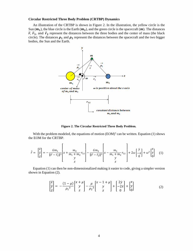
Circular Restricted Three Body Problem (CRTBP) Dynamics
An illustration of the CRTBP is shown in Figure 2. In the illustration, the yellow circle is the
Sun (𝒎𝟏), the blue circle is the Earth (𝒎𝟐), and the green circle is the spacecraft (𝒎). The distances �⃑� , �⃑� 𝟏, and �⃑� 𝟐 represent the distances between the three bodies and the center of mass (the black
circle). The distances 𝝆𝟏 and 𝝆𝟐 represent the distances between the spacecraft and the two bigger
bodies, the Sun and the Earth.
With the problem modeled, the equations of motion (EOM)5 can be written. Equation (1) shows
the EOM for the CRTBP.
Equation (1) can then be non-dimensionalized making it easier to code, giving a simpler version
shown in Equation (2).
[�̈��̈��̈�] = −
(1 − 𝜇)
𝜌13 [
𝑥 + 𝜇𝑦𝑧
] −𝜇
𝜌23 [
𝑥 − 1 + 𝜇𝑦𝑧
] + [2�̇�
−2�̇�0
] + [𝑥𝑦0]
(2)
Figure 2. The Circular Restricted Three Body Problem.
𝑟 ̈ = [�̈��̈��̈�
] = −𝐺𝑚1
‖𝑟 − 𝑟 1‖3
[
𝑥 +𝑚2
𝑚1 + 𝑚2
𝑦𝑧
𝑟12
]
−𝐺𝑚2
‖𝑟 − 𝑟 2‖3
[
𝑥 −𝑚1
𝑚1 + 𝑚2
𝑦𝑧
𝑟12
]
+ 2𝜔 [𝑦
−�̇�̇
0] + 𝜔2 [
𝑥𝑦0] (1)

5
Using the non-dimensionalized EOM in Equation (2), the motion of WFIRST and Starshade
can be propagated over time in the SEL2 system. An example of the motion of WFIRST using the
CRTBP is shown in the Rotating Libration Point (RLP) XY frame in Figure 2. This figure shows
both the LPO and the transfer manifold from Earth to SEL2 (shown in blue) with SEL2 marked as
the red diamond. The blue dots simply represent nodes or marked reference positions in the transfer
and LPO. These nodes are used later for ephemeris corrections purposes.
While Figure 3 gives a CRTBP representation of the behavior of WFIRST at SEL2, the propa-
gation begins to fall apart once Solar Radiation Pressure (SRP) and full ephemeris force models (of
the Sun and the Earth) are added to the design. The resulting motion in full ephemeris with SRP is
shown in Figure 4 in the RLP XY frame. Looking at the figure, we can see that the transfer manifold
and LPO are no longer periodic. The motion has now been disrupted by the addition of SRP and
the ephemeris for the Earth and the Sun. This design was implemented in a MATLAB Module6
that uses the Adaptive Trajectory Design (ATD)7 program.
Figure 3. WFIRST Propagated Motion at SEL2 in the CRTBP shown in the RLP XY Frame.

6
Looking at Figure 4, it is easy to see that the CRTBP motion starts to break down once the SRP
and force models are added to the motion. This is why it is important to do the modeling of WFIRST
and Starshade in a high fidelity force model tool.
WFIRST AND STARSHADE FORMATION FLYING DESIGN
Moving from the CRTBP into a higher fidelity model, the WFIRST nominal mission orbit, and
Starshade’s trajectory that follows the DRM, can be simulated together. WFIRST’s mission orbit
is designed to meet its specific mission requirements at SEL2, and is not to be changed or affected
by the implementation of Starshade. Starshade will follow a reference DRM and remain at a 37,000
km distance from WFIRST during all observations. This distance can vary over the transfer of
Starshade from one observation position to the next, but must meet the observation geometry at the
end of each transfer. To begin the discussion of Starshade’s trajectory design, we show in Figure 5
WFIRST in its nominal mission orbit at SEL2 in the high fidelity force model tool (with SRP and
full gravitational force models for the Earth, Moon, Sun, and Jupiter). The top picture is in the RLP
XY Plane. You can see the Moon’s orbit (the grey circle) and WFIRST’s transfer manifold and
Mission LPO in blue. The bottom picture is in the RLP YZ Plane. This view is from the Earth
looking at SEL2. In the bottom picture you can easily see WFIRST’s evolution through its Quasi-
Halo orbit.
Figure 4. WFIRST Propagated Motion at SEL2 in Full Ephemeris with SRP shown in the RLP
XY Frame.

7
Mission DRM and Ideal Occulter Design
The JPL Starshade team designed a DRM comprised of 48 target stars. Each target star has a
Hipparcos (HIP) number, and a length of observation time. The DRM also included the slew time
and an estimated ΔV to go from one observation to the next. The DRM is planned for 2 years.
Using MATLAB and an automated process called STK COM, the DRM was read into
MATLAB and individual stars were created in a STK scenario that referenced the target stars. STK
has an internal star catalog, and using the HIP number, stars can be inserted into the scenario. With
the DRM stars now in STK, the WFIRST spacecraft can be pointed at the stars at the appropriate
time intervals defined in the DRM.
Within STK, the Analysis Workbench can be used to create a point along the z axis (with align-
ment to the target star) of the WFIRST spacecraft at the desired Starshade distance of 37,000 km.
Using this reference point for each star, an ephemeris in an Earth J2000 frame could be generated
Figure 5. WFIRST Nominal Mission Orbit (in blue) Viewed in the RLP XY Plane (top) and RLP
YZ Plane (bottom) with Moon’s Orbit (in grey) in High Fidelity Force Modeling Tool.

8
for where Starshade needed to be for each specific observation. This ephemeris is the “Starshade
Ideal” ephemeris, and it represents the beginning and end locations for each DRM observation with
respect to WFIRST. A separate spacecraft can be created to read the “Starshade Ideal” ephemeris
and show the individual Starshade observations. Figure 6 shows the “Starshade Ideal” observations
in the red dashes with respect to WFIRST’s mission orbit in blue. Each red dash represents one
observation from the DRM. The dashes are different lengths depending on the length of the obser-
vation specified in the DRM. The DRM has observations planned that vary anywhere from less
than half of a day to more than 6 days.
WFIRST and Starshade Targeted Formation
With the “Starshade Ideal” spacecraft created, the start and end of each observations can be
turned into inertial target locations for use in a Differential Corrector. A separate spacecraft called
Figure 6. “Starshade Ideal” Observations (red) with WFIRST Mission Orbit (blue).
9
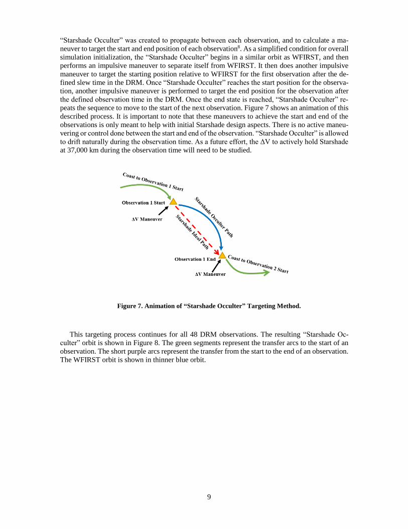
“Starshade Occulter” was created to propagate between each observation, and to calculate a ma-
neuver to target the start and end position of each observation8. As a simplified condition for overall
simulation initialization, the “Starshade Occulter” begins in a similar orbit as WFIRST, and then
performs an impulsive maneuver to separate itself from WFIRST. It then does another impulsive
maneuver to target the starting position relative to WFIRST for the first observation after the de-
fined slew time in the DRM. Once “Starshade Occulter” reaches the start position for the observa-
tion, another impulsive maneuver is performed to target the end position for the observation after
the defined observation time in the DRM. Once the end state is reached, “Starshade Occulter” re-
peats the sequence to move to the start of the next observation. Figure 7 shows an animation of this
described process. It is important to note that these maneuvers to achieve the start and end of the
observations is only meant to help with initial Starshade design aspects. There is no active maneu-
vering or control done between the start and end of the observation. “Starshade Occulter” is allowed
to drift naturally during the observation time. As a future effort, the ΔV to actively hold Starshade
at 37,000 km during the observation time will need to be studied.
This targeting process continues for all 48 DRM observations. The resulting “Starshade Oc-
culter” orbit is shown in Figure 8. The green segments represent the transfer arcs to the start of an
observation. The short purple arcs represent the transfer from the start to the end of an observation.
The WFIRST orbit is shown in thinner blue orbit.
Figure 7. Animation of “Starshade Occulter” Targeting Method.

10
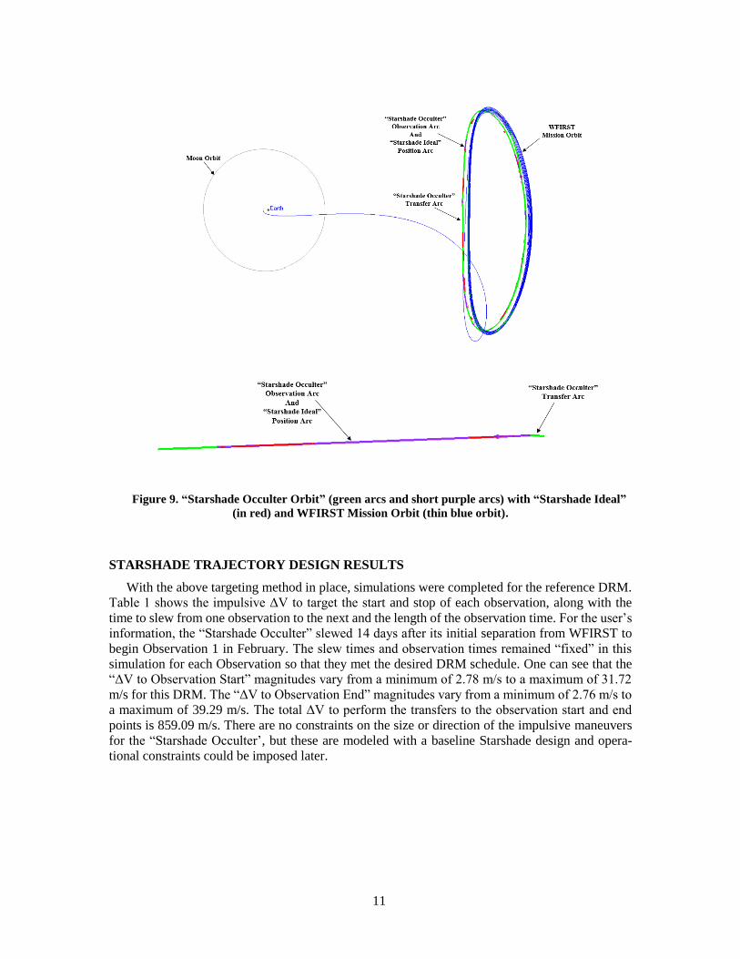
Figure 9 shows the “Starshade Occulter” orbit with the “Starshade Ideal” position arcs (in red)
in the top picture. Looking at the picture on the bottom of this Figure, you can see that the targeting
method was very effective in matching the start and end positions of each observation. The purple
(representing the “Starshade Occulter”) is directly on top of the red (representing the “Starshade
Ideal”).
Figure 8. “Starshade Occulter” Orbit (green arcs and short purple arcs) with WFIRST Mission
Orbit (thin blue orbit).
11
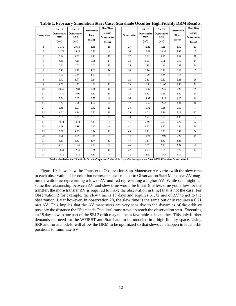
STARSHADE TRAJECTORY DESIGN RESULTS
With the above targeting method in place, simulations were completed for the reference DRM.
Table 1 shows the impulsive ΔV to target the start and stop of each observation, along with the
time to slew from one observation to the next and the length of the observation time. For the user’s
information, the “Starshade Occulter” slewed 14 days after its initial separation from WFIRST to
begin Observation 1 in February. The slew times and observation times remained “fixed” in this
simulation for each Observation so that they met the desired DRM schedule. One can see that the
“ΔV to Observation Start” magnitudes vary from a minimum of 2.78 m/s to a maximum of 31.72
m/s for this DRM. The “ΔV to Observation End” magnitudes vary from a minimum of 2.76 m/s to
a maximum of 39.29 m/s. The total ΔV to perform the transfers to the observation start and end
points is 859.09 m/s. There are no constraints on the size or direction of the impulsive maneuvers
for the “Starshade Occulter’, but these are modeled with a baseline Starshade design and opera-
tional constraints could be imposed later.
Figure 9. “Starshade Occulter Orbit” (green arcs and short purple arcs) with “Starshade Ideal”
(in red) and WFIRST Mission Orbit (thin blue orbit).
12
Table 1. February Simulation Start Case: Starshade Occulter High Fidelity DRM Results.
Figure 10 shows how the Transfer to Observation Start Maneuver ΔV varies with the slew time
to each observation. The color bar represents the Transfer to Observation Start Maneuver ΔV mag-
nitude with blue representing a lower ΔV and red representing a higher ΔV. While one might as-
sume the relationship between ΔV and slew time would be linear (the less time you allow for the
transfer, the more transfer ΔV is required to make the observation in time) that is not the case. For
Observation 2 for example, the slew time is 18 days and requires 31.72 m/s of ΔV to get to the
observation. Later however, in observation 28, the slew time is the same but only requires a 6.21
m/s ΔV. This implies that the ΔV maneuvers are very sensitive to the dynamics of the orbit or
possibly the distance the “Starshade Occulter’ must travel to reach the observation start. Executing
an 18 day slew in one part of the SEL2 orbit may not be as favorable as in another. This only further
demands the need for the WFIRST and Starshade to be modeled in a high fidelity space. Using
SRP and force models, will allow the DRM to be optimized so that slews can happen in ideal orbit
positions to minimize ΔV.

13
Investigating the observations that required an 18 day slew (Observations 2, 10, 16, and 28), we
can see where in the orbit the transfer maneuvers are being executed and analyze the effects of the
system dynamics. Looking at Figure 11, we can see the maneuvers for Observations 16 and 28 are
both occurring near the maximum RLP Y amplitude of the orbit. Observations 2 and 10 are hap-
pening as they are leaving the maximum RLP Y amplitude. Comparatively, the maneuvers are
happening in a relatively similar spot, but they vary drastically in magnitude. Since position didn’t
seem to affect the Transfer to Observation Start Maneuver ΔV’s for these observations, the distance
that the “Starshade Occulter” had to travel to each of these observations was investigated. Table 2
shows the distances (in kilometers) that the “Starshade Occulter” had to travel to get to the Obser-
vations.
Figure 10. Graph of Slew Times for February Simulation Start Case Observations as a function
of Transfer to Observation Start Maneuver ΔV with ΔV magnitude as the color bar.

14
Table 2. February Simulation Start Case: Starshade Occulter Travel
Distances for Observations.
Observation
Difference
in RLP X
(km)
Difference
in RLP Y
(km)
Difference
in RLP Z
(km)
Total
Distance
Traveled
(km)
Transfer to
Observation
Start
ΔV
(m/s)
2 102281.86 340147.25 10526.13 357972.35 31.72
10 10422.46 435343.03 15540.00 435863.34 20.63
16 142478.10 229989.41 45632.15 278870.30 6.89
28 154487.45 102839.51 66390.39 206754.38 9.05
Looking at Table 2, the Transfer to Observation Start Maneuver Δ’s went down as the
Observations continued. The total distance the Starsahde Occulter traveled went down as well
(except for in Observation 10). The other thing of note is that the RLP X values increased as the
Trasnfer to Observation Start Maneuver Δ’s decreased. To understand whether or not this was a
pattern, the Simulation Start time (and hence the start of the Observation schedule) was shifted by
one month from Feburary 11 to March 11. Since the DRM is fixed, and the slew times and
observation times cannot be varied, the only thing that can be changed is when we choose to start
Figure 11. February Simulation Start Case: Observations 2, 10, 16, and 28 locations in the SEL2
Environment (green) with respect to WFIRST (blue).

15
the Observation schedule. Table 3 shows the resultant values from changing the observation
schedule to start in March.
Table 3. March Simulation Start Case: Starshade Occulter High Fidelity DRM Results.
By shifting the start of the Observation schedule by one month, the total ΔV for the “Starshade
Occulter’ DRM is now 840.91 m/s (about 20 m/s less than the February Simulation Start Case).
Looking at Figure 12, we can see that the Transfer ΔV’s for Observation 2, 10, 16, and 28 all have
dropped as well (when compared to the February Simulation Start Case shown in Figure 10).

16
Figure 12. Graph of Slew Times for March Simulation Start Case Observations as a function of
Transfer to Observation Start Maneuver ΔV with ΔV magnitude as the color bar.
Knowing that the Transfer ΔV’s are lower for this new Observation schedule, the RLP distances
and magnitues were investigated again. The results are shown in Table 4.
Table 4. March Simulation Start: Starshade Occulter Travel Distances for Observations.
Observation
Difference
in RLP X
(km)
Difference
in RLP Y
(km)
Difference
in RLP Z
(km)
Total
Distance
Traveled
(km)
Transfer to
Observation
Start
ΔV
(m/s)
2 49655.28 405451.41 26247.15 411084.22 9.08
10 62968.35 291064.49 68481.20 307306.09 18.14
16 34888.64 413189.35 14732.99 415551.50 6.93
28 64191.86 393361.36 12569.08 401063.75 5.85
Looking at the total distance traveled for each observation in Table 4, we can see that even
though the Transfer ΔV magnitudes decreased (except for Observation 16) in the March Simulation
Start case, the distances did not go down (except for Observation 10). The locations for
Observations 2, 10, 16, and 18 were investigated for the March Simulation Start case as well and
are shown in Figure 13.
Looking at Figure 13, we can see that the Transfer to Observation Start Maneuvers are executed
in different places than they were for the February Simulation Start case. For most of these
observations in the February Simulation Start case, these maneuvers happened at the RLP Y
amplitude extremes (or close to them). In the March Simulation Start case, the lower ΔV Transfer
to Observation Start Manuevers appear to occur near RLP XZ plane crossings. This implies that
there may be a relationship between the Transfer to Observation Start Maneuver ΔV magnitudes
and their execution location in the SEL2 environment with respect to WFIRST.

17
Looking only at Observation 2 for both the February and March Simulation Start Cases, the
dynamics of slewing from the end of Observation 1 18 days to Observation 2 was investigated. The
state at the end of Observation 1 was allowed to naturally propagate 18 days to see where the
“Starhsade Occulter” fell with respect to its targeted Observation 2 start position and WFIRST.
Figure 14 shows the results for both the February and March Simulation Start Cases.
Figure 13. March Simulation Start Case: Observations 2, 10, 16, and 28 locations in the SEL2
Environment (green) with respect to WFIRST (blue).
Figure 14. Natural 18 Day Propagation for February and March “Starshade Occulter” (green)
with respect to Targeted Start of Observation 2 (red) and WFIRST (blue)

18
Looking at Figure 14, we can see that the “Starshade Occulter” in the February Simulation Start
Case naturally propagated close to WFIRST and 50,698.90 km away from its desired position to
start Observation 2. In the March Simulation Start Case, however, the “Starshade Occulter”
naturally propagated closer to its desired position to start Observation 2 (15,618.79 km) and
maintained a further distance from WFIRST. The natural dynamics of the “Starshade Occulter” in
the SEL2 environment in the February Simulation Start case forces the “Starshade Occulter” to
execute a large impulsive ΔV maneuver (31.72 m/s from Tables 1 and 2) to meet the starting
position of Observation 2 in 18 days. However, the natural dynamics of the “Starshade Occulter”
in the March Simulation Start Case takes the “Starsahde Occulter” close to its intended target, and
hence results in a smaller impulsive ΔV maneuver (9.08 m/s from Tables 3 and 4). This single
Observation helps emphasize the need to simulate in a high fidelity force model, and also pushes
for very strategic planning of the DRM. If the slew times and observation times are allowed to vary,
the overall ΔV budget for Starshade can be reduced.
To investigate this relationship further, the simulation start time was varied by month for an
entire year. Table 5 shows the total ΔV for the “Starshade Occulter” Transfer to Observation Start
and End Maneuvers for each Simulation Start Time. Looking at the table, we can see that starting
the start of the Observation schedule in January results in a 59 m/s ΔV savings versus starting in
February. Overall however, because the DRM must remain fixed with respect to its slew times and
observation times, the ΔV budget for Starshade would need to remain in the 800 m/s range if this
desired DRM does not change.
Table 5: Total “Starshade Occulter” ΔV for each Simulation Start Time
The Transfer to Observation Start Maneuver ΔV’s were then compared for Observations 2, 10,
16, and 28 for each month, and their locations in the SEL2 were also investigated. These minimum
Transfer to Observation Start Maneuver ΔV results and locations are shown in Figure 15. The line
in the graphs are a fitted polynomial to show how the Transfer to Observation Start Maneuver ΔV’s
rise and fall over each month. Looking at the figure, we can see that the maneuvers are being
executed relatively close to the RLP Y extremes. This may be a coincidence or it may simply fall
back to the natural dynamics of the “Starshade Occulter” with respect to WFIRST and its targeted
starting position for these observations.

19
Looking at Figure 15, we can see that there are minimum Transfer to Observation Start
Maneuver ΔV’s that occur among the Simulation Start times. For Observation 2, the minimum
occurs in the August Simulation Start Case. For Observation 10, the minimum occurs in the May
Simulation Start Case. For Observation 16, the February Simulation Start Case actually has the
minimum. Finally, for Observation 28, the minimum occurs in the September Simulation Start
Case.
If the DRM is allowed to change, these observations could be scheduled to occur around these
minimum ΔV opportunities in order to reduce the overall Starshade ΔV. By allowing the slew times
and observation times to vary, the ΔV for each observation may drop significantly and is something
to be investigated in the future.
CONCLUSIONS
The results have shown that designing the “Starshade Occulter” to meet a fixed DRM can result
in varying Transfer to Observation Start ΔV magnitudes for each observation. The natural dynam-
ics of the “Starshade Occulter” can either help minimize this ΔV, or require a significant ΔV in
order to achieve the desired Observation starting positions. The minimum ΔV Transfer to Obser-
vation Start Maneuvers are being directed in a way that places the “Starshade Occulter” onto a
manifold to places it closer to its intended Observation starting position while also keeping it sep-
arated from WFIRST. The higher ΔV Transfer to Observation Start Maneuvers are fighting against
the dynamics in order to reach the Observation point in the desired time.
Figure 15. Observations 2 (blue), 6 (red), 10 (yellow), and 28 (green) Transfer to Observation
Start Maneuver ΔV’s for each Simulation Start Time.
20
Once the dynamics are understood more clearly, an optimization can be performed to help min-
imize the total ΔV for the “Starshade Occulter”, thereby reducing the wet mass and total mass of
Starshade’s design. Varying the Simulation Start Time resulted in significant ΔV savings for the
“Starshade Occulter”, and the planning/timing of the slews and observations in the DRM should be
investigated further to help minimize the total ΔV.
SUMMARY
A high fidelity model was used to simulate a Starshade Occulter flying with WFIRST following
a fixed DRM. The impulsive ΔV maneuvers to transfer from the start and end of one Observation
to the next were determined as well. By varying the Simulation Start Times (and hence the begin-
ning of the DRM), the total ΔV for the “Starshade Occulter” can be minimized. The results also
showed that the natural dynamics of the “Starshade Occulter” can either minimize or maximize the
Transfer to Observation Start ΔV. The SEL2 environment can take the “Starshade Occulter” to
close to its intended targets, or far away from them. A deeper investigation into the dynamics at
each Observation, and allowing the DRM to vary the slew times and observation times, can help
optimize the fuel savings for Starshade. By helping the “Starshade Occulter” follow natural mani-
folds to transfer close to each Observation start, the ΔV can be minimized resulting in significant
mass savings for Starshade.
ACKNOWLEDGMENTS
I would like acknowledge Lauren McManus9 and Natasha Bosanac10 for their help in this anal-
ysis.
1 NASA WFIRST Mission Website, https://wfirst.gsfc.nasa.gov/about.html
2 Seager, Sara, Warfield, K. Cash, W., Domagal-Goldman, S., Kasdin, N. J., Kuchner, M., Roberge, A., Shaklam, S.,
Sparks, W., Thomson, M., Turnbull, M., Lisman, D., Baran, R., Bauman, R., Cady, E., Henegham, C., Martin, S., Scharf,
D., Trabert, R., Webb, D., Zarifian, P., “Exo-S: Starshade Probe-Class Exoplanet Direct Imagining Mission Concept
Final Report” https://exoplanets.nasa.gov/stdt/Exo-S_Starshade_Probe_Class_Final_Report_150312_URS250118.pdf,
March 2015.
3 Lisman, Doug, “WFIRST-Starshade Overview and Introduction to Accommodations Issues”. DRM Internal Memo.
August 09. 2016.
4 Millard, Lindsay D., Howell, Kathleen C. “Optimal reconfiguration maneuvers for spacecraft imaging arrays in multi-
body regimes”. http://www.sciencedirect.com/science/article/pii/S0094576508001884 December 2008
5 Pavlak, Thomas A. “Mission Design Applications in the Earth-Moon System: Transfer Trajectories and Stationkeeping”
https://engineering.purdue.edu/people/kathleen.howell.1/Publications/Masters/2010_Pavlak.pdf May 2010.
6 Bosanac, Natasha, “Sun-Earth Libration Point Trajectory Design Module Tutorial” Version 1. December 2016.
7 Folta, David, Haapala, Amanda, Pavlak, Tom, Howell, Kathleen “Adaptive Trajectory Design (ATD) / GSFC IRAD”
https://engineering.purdue.edu/people/kathleen.howell.1/Gallery/Posters/these_images/IRAD_2013.pdf August 2013.
8 Folta, D., Lowe, J., “Formation Flying Of A Telescope/Occulter System With Large Separations In An L2 Libration
Orbit”. IAC-08-C1.6.2
9 McManus, Lauren, [email protected], Analytical Graphics, Inc. 220 Valley Creek Blvd., Exton, PA 19314, USA
10 Bosanac, Natasha, [email protected], University of Colorado Boulder, Colorado Center for Astrody-
namics Research (CCAR), Boulder, CO 80309, USA
REFERENCES


![Orbit type: Sun Synchronous Orbit ] Orbit height: …...Orbit type: Sun Synchronous Orbit ] PSLV - C37 Orbit height: 505km Orbit inclination: 97.46 degree Orbit period: 94.72 min ISL](https://img.dokumen.tips/doc/110x75/5f781053e671b364921403bc/orbit-type-sun-synchronous-orbit-orbit-height-orbit-type-sun-synchronous.jpg)