Embed Size (px)
Citation preview

Understanding the Finite-Difference Time-DomainMethod
John B. Schneider
April 5, 2017

ii

Contents
1 Numeric Artifacts 71.1 Introduction . . . . . . . . . . . . . . . . . . . . . . . . . . . . . . . . . . . . . . 71.2 Finite Precision . . . . . . . . . . . . . . . . . . . . . . . . . . . . . . . . . . . . 81.3 Symbolic Manipulation . . . . . . . . . . . . . . . . . . . . . . . . . . . . . . . . 11
2 Brief Review of Electromagnetics 132.1 Introduction . . . . . . . . . . . . . . . . . . . . . . . . . . . . . . . . . . . . . . 132.2 Coulomb’s Law and Electric Field . . . . . . . . . . . . . . . . . . . . . . . . . . 132.3 Electric Flux Density . . . . . . . . . . . . . . . . . . . . . . . . . . . . . . . . . 152.4 Static Electric Fields . . . . . . . . . . . . . . . . . . . . . . . . . . . . . . . . . 172.5 Gradient, Divergence, and Curl . . . . . . . . . . . . . . . . . . . . . . . . . . . . 182.6 Laplacian . . . . . . . . . . . . . . . . . . . . . . . . . . . . . . . . . . . . . . . 212.7 Gauss’s and Stokes’ Theorems . . . . . . . . . . . . . . . . . . . . . . . . . . . . 242.8 Electric Field Boundary Conditions . . . . . . . . . . . . . . . . . . . . . . . . . 252.9 Conductivity and Perfect Electric Conductors . . . . . . . . . . . . . . . . . . . . 252.10 Magnetic Fields . . . . . . . . . . . . . . . . . . . . . . . . . . . . . . . . . . . . 262.11 Magnetic Field Boundary Conditions . . . . . . . . . . . . . . . . . . . . . . . . . 272.12 Summary of Static Fields . . . . . . . . . . . . . . . . . . . . . . . . . . . . . . . 272.13 Time Varying Fields . . . . . . . . . . . . . . . . . . . . . . . . . . . . . . . . . . 282.14 Summary of Time-Varying Fields . . . . . . . . . . . . . . . . . . . . . . . . . . 292.15 Wave Equation in a Source-Free Region . . . . . . . . . . . . . . . . . . . . . . . 292.16 One-Dimensional Solutions to the Wave Equation . . . . . . . . . . . . . . . . . 30
3 Introduction to the FDTD Method 333.1 Introduction . . . . . . . . . . . . . . . . . . . . . . . . . . . . . . . . . . . . . . 333.2 The Yee Algorithm . . . . . . . . . . . . . . . . . . . . . . . . . . . . . . . . . . 343.3 Update Equations in 1D . . . . . . . . . . . . . . . . . . . . . . . . . . . . . . . 353.4 Computer Implementation of a One-Dimensional
FDTD Simulation . . . . . . . . . . . . . . . . . . . . . . . . . . . . . . . . . . . 393.5 Bare-Bones Simulation . . . . . . . . . . . . . . . . . . . . . . . . . . . . . . . . 413.6 PMC Boundary in One Dimension . . . . . . . . . . . . . . . . . . . . . . . . . . 443.7 Snapshots of the Field . . . . . . . . . . . . . . . . . . . . . . . . . . . . . . . . . 453.8 Additive Source . . . . . . . . . . . . . . . . . . . . . . . . . . . . . . . . . . . 483.9 Terminating the Grid . . . . . . . . . . . . . . . . . . . . . . . . . . . . . . . . . 503.10 Total-Field/Scattered-Field Boundary . . . . . . . . . . . . . . . . . . . . . . . . 53
iii

iv CONTENTS
3.11 Inhomogeneities . . . . . . . . . . . . . . . . . . . . . . . . . . . . . . . . . . . 603.12 Lossy Material . . . . . . . . . . . . . . . . . . . . . . . . . . . . . . . . . . . . 66
4 Improving the FDTD Code 754.1 Introduction . . . . . . . . . . . . . . . . . . . . . . . . . . . . . . . . . . . . . . 754.2 Arrays and Dynamic Memory Allocation . . . . . . . . . . . . . . . . . . . . . . 754.3 Macros . . . . . . . . . . . . . . . . . . . . . . . . . . . . . . . . . . . . . . . . 774.4 Structures . . . . . . . . . . . . . . . . . . . . . . . . . . . . . . . . . . . . . . . 804.5 Improvement Number One . . . . . . . . . . . . . . . . . . . . . . . . . . . . . . 864.6 Modular Design and Initialization Functions . . . . . . . . . . . . . . . . . . . . . 904.7 Improvement Number Two . . . . . . . . . . . . . . . . . . . . . . . . . . . . . . 954.8 Compiling Modular Code . . . . . . . . . . . . . . . . . . . . . . . . . . . . . . 1024.9 Improvement Number Three . . . . . . . . . . . . . . . . . . . . . . . . . . . . . 103
5 Scaling FDTD Simulations to Any Frequency 1155.1 Introduction . . . . . . . . . . . . . . . . . . . . . . . . . . . . . . . . . . . . . . 1155.2 Sources . . . . . . . . . . . . . . . . . . . . . . . . . . . . . . . . . . . . . . . . 115
5.2.1 Gaussian Pulse . . . . . . . . . . . . . . . . . . . . . . . . . . . . . . . . 1155.2.2 Harmonic Sources . . . . . . . . . . . . . . . . . . . . . . . . . . . . . . 1165.2.3 The Ricker Wavelet . . . . . . . . . . . . . . . . . . . . . . . . . . . . . 117
5.3 Mapping Frequencies to Discrete Fourier Transforms . . . . . . . . . . . . . . . . 1205.4 Running Discrete Fourier Transform (DFT) . . . . . . . . . . . . . . . . . . . . . 1215.5 Real Signals and DFT’s . . . . . . . . . . . . . . . . . . . . . . . . . . . . . . . . 1235.6 Amplitude and Phase from Two Time-Domain Samples . . . . . . . . . . . . . . 1265.7 Conductivity . . . . . . . . . . . . . . . . . . . . . . . . . . . . . . . . . . . . . 1285.8 Transmission Coefficient for a Planar Interface . . . . . . . . . . . . . . . . . . . 132
5.8.1 Transmission through Planar Interface . . . . . . . . . . . . . . . . . . . . 1345.8.2 Measuring the Transmission Coefficient Using FDTD . . . . . . . . . . . 135
6 Differential-Equation Based ABC’s 1456.1 Introduction . . . . . . . . . . . . . . . . . . . . . . . . . . . . . . . . . . . . . . 1456.2 The Advection Equation . . . . . . . . . . . . . . . . . . . . . . . . . . . . . . . 1456.3 Terminating the Grid . . . . . . . . . . . . . . . . . . . . . . . . . . . . . . . . . 1466.4 Implementation of a First-Order ABC . . . . . . . . . . . . . . . . . . . . . . . . 1486.5 ABC Expressed Using Operator Notation . . . . . . . . . . . . . . . . . . . . . . 1536.6 Second-Order ABC . . . . . . . . . . . . . . . . . . . . . . . . . . . . . . . . . . 1566.7 Implementation of a Second-Order ABC . . . . . . . . . . . . . . . . . . . . . . 158
7 Dispersion, Impedance, Reflection, and Transmission 1617.1 Introduction . . . . . . . . . . . . . . . . . . . . . . . . . . . . . . . . . . . . . . 1617.2 Dispersion in the Continuous World . . . . . . . . . . . . . . . . . . . . . . . . . 1617.3 Harmonic Representation of the FDTD Method . . . . . . . . . . . . . . . . . . . 1627.4 Dispersion in the FDTD Grid . . . . . . . . . . . . . . . . . . . . . . . . . . . . 1657.5 Numeric Impedance . . . . . . . . . . . . . . . . . . . . . . . . . . . . . . . . . . 1697.6 Analytic FDTD Reflection and Transmission Coefficients . . . . . . . . . . . . . . 169

CONTENTS v
7.7 Reflection from a PEC . . . . . . . . . . . . . . . . . . . . . . . . . . . . . . . . 1737.8 Interface Aligned with an Electric-Field Node . . . . . . . . . . . . . . . . . . . . 175
8 Two-Dimensional FDTD Simulations 1818.1 Introduction . . . . . . . . . . . . . . . . . . . . . . . . . . . . . . . . . . . . . . 1818.2 Multidimensional Arrays . . . . . . . . . . . . . . . . . . . . . . . . . . . . . . . 1818.3 Two Dimensions: TMz Polarization . . . . . . . . . . . . . . . . . . . . . . . . . 1858.4 TMz Example . . . . . . . . . . . . . . . . . . . . . . . . . . . . . . . . . . . . . 1898.5 The TFSF Boundary for TMz Polarization . . . . . . . . . . . . . . . . . . . . . . 2028.6 TMz TFSF Boundary Example . . . . . . . . . . . . . . . . . . . . . . . . . . . . 2088.7 TEz Polarization . . . . . . . . . . . . . . . . . . . . . . . . . . . . . . . . . . . 2208.8 PEC’s in TEz and TMz Simulations . . . . . . . . . . . . . . . . . . . . . . . . . 2248.9 TEz Example . . . . . . . . . . . . . . . . . . . . . . . . . . . . . . . . . . . . . 227
9 Three-Dimensional FDTD 2419.1 Introduction . . . . . . . . . . . . . . . . . . . . . . . . . . . . . . . . . . . . . . 2419.2 3D Arrays in C . . . . . . . . . . . . . . . . . . . . . . . . . . . . . . . . . . . . 2419.3 Governing Equations and the 3D Grid . . . . . . . . . . . . . . . . . . . . . . . . 2449.4 3D Example . . . . . . . . . . . . . . . . . . . . . . . . . . . . . . . . . . . . . . 2529.5 TFSF Boundary . . . . . . . . . . . . . . . . . . . . . . . . . . . . . . . . . . . . 2679.6 TFSF Demonstration . . . . . . . . . . . . . . . . . . . . . . . . . . . . . . . . . 2729.7 Unequal Spatial Steps . . . . . . . . . . . . . . . . . . . . . . . . . . . . . . . . . 282
10 Dispersive Material 28910.1 Introduction . . . . . . . . . . . . . . . . . . . . . . . . . . . . . . . . . . . . . . 28910.2 Constitutive Relations and Dispersive Media . . . . . . . . . . . . . . . . . . . . . 290
10.2.1 Drude Materials . . . . . . . . . . . . . . . . . . . . . . . . . . . . . . . 29110.2.2 Lorentz Material . . . . . . . . . . . . . . . . . . . . . . . . . . . . . . . 29210.2.3 Debye Material . . . . . . . . . . . . . . . . . . . . . . . . . . . . . . . . 293
10.3 Debye Materials Using the ADE Method . . . . . . . . . . . . . . . . . . . . . . . 29410.4 Drude Materials Using the ADE Method . . . . . . . . . . . . . . . . . . . . . . . 29610.5 Magnetically Dispersive Material . . . . . . . . . . . . . . . . . . . . . . . . . . . 29810.6 Piecewise Linear Recursive Convolution . . . . . . . . . . . . . . . . . . . . . . . 30110.7 PLRC for Debye Material . . . . . . . . . . . . . . . . . . . . . . . . . . . . . . . 305
11 Perfectly Matched Layer 30711.1 Introduction . . . . . . . . . . . . . . . . . . . . . . . . . . . . . . . . . . . . . . 30711.2 Lossy Layer, 1D . . . . . . . . . . . . . . . . . . . . . . . . . . . . . . . . . . . . 30811.3 Lossy Layer, 2D . . . . . . . . . . . . . . . . . . . . . . . . . . . . . . . . . . . . 31011.4 Split-Field Perfectly Matched Layer . . . . . . . . . . . . . . . . . . . . . . . . . 31211.5 Un-Split PML . . . . . . . . . . . . . . . . . . . . . . . . . . . . . . . . . . . . . 31511.6 FDTD Implementation of Un-Split PML . . . . . . . . . . . . . . . . . . . . . . . 318

vi CONTENTS
12 Acoustic FDTD Simulations 32312.1 Introduction . . . . . . . . . . . . . . . . . . . . . . . . . . . . . . . . . . . . . . 32312.2 Governing FDTD Equations . . . . . . . . . . . . . . . . . . . . . . . . . . . . . 32512.3 Two-Dimensional Implementation . . . . . . . . . . . . . . . . . . . . . . . . . . 328
13 Parallel Processing 33113.1 Threads . . . . . . . . . . . . . . . . . . . . . . . . . . . . . . . . . . . . . . . . 33113.2 Thread Examples . . . . . . . . . . . . . . . . . . . . . . . . . . . . . . . . . . . 33313.3 Message Passing Interface . . . . . . . . . . . . . . . . . . . . . . . . . . . . . . 34013.4 Open MPI Basics . . . . . . . . . . . . . . . . . . . . . . . . . . . . . . . . . . . 34113.5 Rank and Size . . . . . . . . . . . . . . . . . . . . . . . . . . . . . . . . . . . . . 34313.6 Communicating Between Processes . . . . . . . . . . . . . . . . . . . . . . . . . 344
14 Near-to-Far-Field Transformation 35114.1 Introduction . . . . . . . . . . . . . . . . . . . . . . . . . . . . . . . . . . . . . . 35114.2 The Equivalence Principle . . . . . . . . . . . . . . . . . . . . . . . . . . . . . . 35114.3 Vector Potentials . . . . . . . . . . . . . . . . . . . . . . . . . . . . . . . . . . . 35214.4 Electric Field in the Far-Field . . . . . . . . . . . . . . . . . . . . . . . . . . . . . 35914.5 Simpson’s Composite Integration . . . . . . . . . . . . . . . . . . . . . . . . . . . 36314.6 Collocating the Electric and Magnetic Fields: The Geometric Mean . . . . . . . . 36314.7 NTFF Transformations Using the Geometric Mean . . . . . . . . . . . . . . . . . 366
14.7.1 Double-Slit Radiation . . . . . . . . . . . . . . . . . . . . . . . . . . . . 36614.7.2 Scattering from a Circular Cylinder . . . . . . . . . . . . . . . . . . . . . 37014.7.3 Scattering from a Strongly Forward-Scattering Sphere . . . . . . . . . . . 371
A Construction of Fourth-Order Central Differences A.377
B Generating a Waterfall Plot and Animation B.379
C Rendering and Animating Two-Dimensional Data C.383
D Notation D.387
E PostScript Primer E.389E.1 Introduction . . . . . . . . . . . . . . . . . . . . . . . . . . . . . . . . . . . . . . E.389E.2 The PostScript File . . . . . . . . . . . . . . . . . . . . . . . . . . . . . . . . . . E.390E.3 PostScript Basic Commands . . . . . . . . . . . . . . . . . . . . . . . . . . . . . E.390
Index 403

Chapter 1
Numeric Artifacts
1.1 IntroductionVirtually all solutions to problems in electromagnetics require the use of a computer. Even whenan analytic or “closed form” solution is available which is nominally exact, one typically must usea computer to translate that solution into numeric values for a given set of parameters. Becauseof inherent limitations in the way numbers are stored in computers, some errors will invariably bepresent in the resulting solution. These errors will typically be small but they are an artifact aboutwhich one should be aware. Here we will discuss a few of the consequences of finite precision.
Later we will be discussing numeric solutions to electromagnetic problems which are basedon the finite-difference time-domain (FDTD) method. The FDTD method makes approximationsthat force the solutions to be approximate, i.e., the method is inherently approximate. The resultsobtained from the FDTD method would be approximate even if we used computers that offeredinfinite numeric precision. The inherent approximations in the FDTD method will be discussed insubsequent chapters.
With numerical methods there is one note of caution which one should always keep in mind.Provided the implementation of a solution does not fail catastrophically, a computer is alwayswilling to give you a result. You will probably find there are times when, to get your programsimply to run, the debugging process is incredibly arduous. When your program does run, thenatural assumption is that all the bugs have been fixed. Unfortunately that often is not the case.Getting the program to run is one thing, getting correct results is another. And, in fact, gettingaccurate results is yet another thing—your solution may be correct for the given implementation,but the implementation may not be one which is capable of producing sufficiently accurate results.Therefore, the more ways you have to test your implementation and your solution, the better. Forexample, a solution may be obtained at one level of discretization and then another solution usinga finer discretization. If the two solutions are not sufficiently close, one has not yet converged tothe “true” solution and a finer discretization must be used or, perhaps, there is some systemic errorin the implementation. The bottom line: just because a computer gives you an answer does notmean that answer is correct.
Lecture notes by John Schneider. numerical-issues.tex
7

8 CHAPTER 1. NUMERIC ARTIFACTS
1.2 Finite PrecisionIf we sum one-eleventh eleven times we know that the result is one, i.e., 1/11 + 1/11 + 1/11 +1/11 + 1/11 + 1/11 + 1/11 + 1/11 + 1/11 + 1/11 = 1. But is that true on a computer? Considerthe C program shown in Program 1.1.
Program 1.1 oneEleventh.c: Test if 1/11 + 1/11 + 1/11 + 1/11 + 1/11 + 1/11 + 1/11 +1/11 + 1/11 + 1/11 equals 1.
1 /* Is summing 1./11. ten times == 1.0? */2 #include <stdio.h>3
4 int main() 5 float a;6
7 a = 1.0 / 11.0;8
9 if (a + a + a + a + a + a + a + a + a + a + a == 1.0)10 printf("Equal.\n");11 else12 printf("Not equal.\n");13
14 return 0;15
In this program the float variable a is set to one-eleventh. In line 9 the sum of eleven a’s iscompared to one. If they are equal, the program prints “Equal” but prints “Not equal” otherwise.The output of this program is “Not equal.” Thus, to a computer (at least one running a languagetypically used in the solution of electromagnetics problems), the sum of one-eleventh eleven timesis not equal to one. It is worth noting that had line 9 been written a=1/11;, a would have been setto zero since integer math would be used to evaluate the division. By using a = 1.0 / 11.0;,the computer uses floating-point math.
The floating-point data types in C or FORTRAN can only store a finite number of digits. Onmost machines four bytes (32 binary digits or bits) are used for single-precision numbers andeight bytes (64 digits) are used for double precision. Returning to the sum of one-elevenths, asan extreme example, assumed that a computer can only store two decimal digits. One eleventh isequal to 0.09090909. . . Thus, to two decimal places one-eleventh would be approximated by 0.09.Summing this eleven times yields
0.09 + 0.09 + 0.09 + 0.09 + 0.09 + 0.09 + 0.09 + 0.09 + 0.09 + 0.09 + 0.09 = 0.99
which is clearly not equal to one. If the number is stored with more digits, the result becomescloser to one, but it never gets there. Both the decimal and binary floating-point representationof one-eleventh have an infinite number of digits. Thus, when attempting to store one-eleventh

1.2. FINITE PRECISION 9
in a computer the number has to be truncated so that the computer stores an approximation ofone-eleventh. Because of this truncation summing one-eleventh eleven times does not yield one.
Since 1/10 is equal to 0.1, it might appear this number can be stored with a finite numberof digits. Although one-tenth has a finite number of digits when written in base ten (decimalrepresentation), it has an infinite number of digits when written in base two (binary representation).
In a floating-point decimal number each digit represents the number of a particular power often. Letting a blank represent a digit, a decimal number can be thought of in the follow way:
. . . . . . .
103 102 101 100 10−1 10−2 10−3 10−4
Each digits tells how many of a particular power of 10 there is in a number. The decimal pointserves as the dividing line between negative and non-negative exponents. Binary numbers aresimilar except each digit represents a power or two:
. . . . . . .
23 22 21 20 2−1 2−2 2−3 2−4
The base-ten number 0.110 is simply 1× 10⁻¹. To obtain the same value using binary numbers wehave to take 2−4 + 2−5 + 2−8 + 2−9 + . . ., i.e., an infinite number of binary digits. Another way ofwriting this is
0.110 = 0.0001100110011001100110011 . . .2 .
As before, when this is stored in a computer, the number has to be truncated. The stored value isno longer precisely equal to one-tenth. Summing ten of these values does not yield one (althoughthe difference is very small).
The details of how floating-point values are stored in a computer are not a primary concern.However, it is helpful to know how bits are allocated. Numbers are stored in exponential form andthe standard allocation of bits is:
total bits sign mantissa exponentsingle precision 32 1 23 8double precision 64 1 52 11
Essentially the exponent gives the magnitude of the number while the mantissa gives the digits ofthe number—the mantissa determines the precision. The more digits available for the mantissa,the more precisely a number can be represented. Although a double-precision number has twiceas many total bits as a single-precision number, it uses 52 bits for the mantissa whereas a single-precision number uses 23. Therefore double-precision numbers actually offer more than twice theprecision of single-precision numbers. A mantissa of 23 binary digits corresponds to a little lessthan seven decimal digits. This is because 223 is 8,388,608, thus 23 binary digits can representnumbers between 0 and 8,388,607. On the other hand, a mantissa of 52 binary digits correspondsto a value with between 15 and 16 decimal digits (252 = 4,503,599,627,370,496).
For the exponent, a double-precision number has three more bits than a single-precision num-ber. It may seem as if the double-precision exponent has been short-changed as it does not havetwice as many bits as a single-precision number. However, keep in mind that the exponent repre-sents the size of a number. Each additional bit essentially doubles the number of values that can berepresented. If the exponent had nine bits, it could represent numbers which were twice as large

10 CHAPTER 1. NUMERIC ARTIFACTS
as single-precision numbers. The three additional bits that a double-precision number possessesallows it to represent exponents which are eight times larger than single-precision numbers. Thistranslates into numbers which are 256 times larger (or smaller) in magnitude than single-precisionnumbers.
Consider the following equationa+ b = a.
From mathematics we know this equation can only be satisfied if b is zero. However, using com-puters this equation can be true, i.e., b makes no contribution to a, even when b is non-zero.
When numbers are added or subtracted, their mantissas are shifted until their exponents areequal. At that point the mantissas can be directly added or subtracted. However, if the differencein the exponents is greater than the length of the mantissa, then the smaller number will not haveany affect when added to or subtracted from the larger number. The code fragment shown inFragment 1.2 illustrates this phenomenon.
Fragment 1.2 Code fragment to test if a non-zero b can satisfy the equation a+ b = a.
1 float a = 1.0, b = 0.5, c;2
3 c = a + b;4
5 while(c != a) 6 b = b / 2.0;7 c = a + b;8 9
10 printf("%12g %12g %12g\n",a,b,c);
Here a is initialized to one while b is set to one-half. The variable c holds the sum of a and b.The while-loop starting on line 5 will continue as long as c is not equal to a. In the body of theloop, b is divided by 2 and c is again set equal to a+ b. If the computer had infinite precision, thiswould be an infinite loop. The value of b would become vanishingly small, but it would never bezero and hence a+ b would never equal a. However, the loop does terminate and the output of theprintf() statement in line 10 is:
1 5.96046e-08 1
This shows that both a and c are unity while b has a value of 5.96046× 10⁻⁸. Note that this valueof b corresponds to 1× 2−24. When b has this value, the exponents of a and b differ by more than23 (a is 1× 20).
One more example serves to illustrate the less-than-obvious ways in which finite precision cancorrupt a calculation. Assume the variable a is set equal to 2. Taking the square root of a and thensquaring a should yield a result which is close to 2 (ideally it would be 2, but since
√2 has an
infinite number of digits, some accuracy will be lost). However, what happens if the square root is

1.3. SYMBOLIC MANIPULATION 11
taken 23 times and then the number is squared 23 times? We would hope to get a result close totwo, but that is not the case. The program shown in Program 1.3 allows us to test this scenario.
Program 1.3 rootTest.c: Take the square root of a number repeatedly and then squaring thenumber an equal number of times.
1 /* Square-root test. */2 #include <math.h> // needed for sqrt()3 #include <stdio.h>4
5 #define COUNT 236
7 int main() 8 float a = 2.0;9 int i;
10
11 for (i = 0; i < COUNT; i++)12 a = sqrt(a); // square root of a13
14 for (i = 0; i < COUNT; i++)15 a = a * a; // a squared16
17 printf("%12g\n",a);18
19 return 0;20
The program output is one, i.e., the result is a = 1.0. Each time the square root is taken, the valuegets closer and closer to unity. Eventually, because of truncation error, the computer thinks thenumber is unity. At that point no amount of squaring the number will change it.
1.3 Symbolic ManipulationWhen using languages which are typically used in numerical analysis (such as C, C++, FOR-TRAN, or even Matlab), truncation error is unavoidable. The ratio of the circumference of a circleto its diameter is the number π = 3.141592 . . . This is an irrational number with an infinite num-ber of digits. Thus one cannot store the exact numeric value of π in a computer. Instead, onemust use an approximation consisting of a finite number of digits. However, there are softwarepackages, such a Mathematica, that allow one to manipulate symbols. Within Mathematica, ifa person writes Pi, Mathematica “knows” symbolically what that means. For example, the co-sine of 10000000001*Pi is identically negative one. Similarly, one could write Sqrt[2].Mathematica knows that the square of this is identically 2. Unfortunately, though, such symbolicmanipulations are incredibly expensive in terms of computational resources. Many cutting-edge

12 CHAPTER 1. NUMERIC ARTIFACTS
problems in electromagnetics can involve hundreds of thousand or even millions of unknowns. Todeal with these large amounts of data it is imperative to be as efficient—both in terms of memoryand computation time—as possible. Mathematica is wonderful for many things, but it is not theright tool for solving large numeric problems.
In Matlab one can write pi as a shorthand representation of π. However, this representation ofπ is different from that used in Mathematica. In Matlab, pi is essentially the same as the numericrepresentation—it is just more convenient to write pi than all the numeric digits. In C, providedyou have included the header file math.h, you can use M PI as a shorthand for π. Looking inmath.h reveals the following statement:
# define M_PI 3.14159265358979323846 /* pi */
This is similar to what is happening in Matlab. Matlab only knows what the numeric value ofpi is and that numeric value is a truncated version of the true value. Thus, taking the cosine of10000000001*pi yields −0.99999999999954 instead of the exact value of −1 (but, of course,the difference is trivial in this case).

Chapter 2
Brief Review of Electromagnetics
2.1 IntroductionThe specific equations on which the finite-difference time-domain (FDTD) method is based willbe considered in some detail later. The goal here is to remind you of the physical significance ofthe equations to which you have been exposed in previous courses on electromagnetics.
In some sense there are just a few simple premises which underlie all electromagnetics. Onecould argue that electromagnetics is simply based on the following:
1. Charge exerts force on other charge.
2. Charge in motion exerts a force on other charge in motion.
3. All material is made up of charged particles.
Of course translating these premises into a corresponding mathematical framework is not trivial.However one should not lose sight of the fact that the math is trying to describe principles that areconceptually rather simple.
2.2 Coulomb’s Law and Electric FieldCoulomb studied the electric force on charged particles. As depicted in Fig. 2.1, given two discreteparticles carrying chargeQ1 andQ2, the force experienced byQ2 due toQ1 is along the line joiningQ1 and Q2. The force is proportional to the charges and inversely proportional to the square of thedistance between the charges. A proportionality constant is needed to obtain Coulomb’s law whichgives the equation of the force on Q2 due to Q1:
F12 = a121
4πε0
Q1Q2
R212
(2.1)
where a12 is a unit vector pointing from Q1 to Q2, R12 is the distance between the charges, and1/4πε0 is the proportionality constant. The constant ε0 is known as the permittivity of free space
Lecture notes by John Schneider. em-review.tex
13

14 CHAPTER 2. BRIEF REVIEW OF ELECTROMAGNETICS
+Q
1
Q2
F12 = Q2
E
Figure 2.1: The force experienced by charge Q2 due to charge Q1 is along the line which passthrough both charges. The direction of the force is dictate by the signs of the charges. Electric fieldis assumed to point radially away from positive charges as is indicated by the lines pointing awayfrom Q1 (which is assumed here to be positive).
and equals approximately 8.854 × 10⁻¹² F/m. Charge is expressed in units of Coulombs (C) andcan be either negative or positive. When the two charges have like signs, the force will be repulsive:F12 will be parallel to a12. When the charges are of opposite sign, the force will be attractive sothat F12 will be anti-parallel to a12.
There is a shortcoming with (2.1) in that it implies action at a distance. It appears from thisequation that the force F12 is established instantly. From this equation one could assume that achange in the distance R12 results in an instantaneous change in the force F12, but this is not thecase. A finite amount of time is required to communicate the change in location of one charge tothe other charge (similarly, it takes a finite amount of time to communicate a change in the quantityof one charge to the other charge). To overcome this shortcoming it is convenient to employ theconcept of fields. Instead of Q1 producing a force directly on Q2, Q1 is said to produce a field.This field then produces a force on Q2. The field produced by Q1 is independent of Q2—it existswhether or not Q2 is there to experience it.
In the static case, the field approach does not appear to have any advantage over the direct useof Coulomb’s law. This is because for static charges Coulomb’s law is correct. Fields must betime-varying for the distinction to arise. Nevertheless, to be consistent with the time-varying case,fields are used in the static case as well. The electric field produced by the point charge Q1 is
E1 = arQ1
4πε0r2(2.2)
where ar is a unit vector which points radially away from the charge and r is the distance from thecharge. The electric field has units of volts per meter (V/m).
To find the force on Q2, one merely takes the charge times the electric field: F12 = Q2E1. Ingeneral, the force on any charge Q is the product of the charge and the electric field at which thecharge is present, i.e., F = QE.

2.3. ELECTRIC FLUX DENSITY 15
2.3 Electric Flux DensityAll material is made up of charged particles. The material may be neutral overall because it hasas many positive charges as negative charges. Nevertheless, there are various ways in which thepositive and negative charges may shift slightly within the material, perhaps under the influence ofan electric field. The resulting charge separation will have an effect on the overall electric field.Because of this it is often convenient to introduce a new field known as the electric flux density, D,which has units of Coulombs per square meter (C/m2).∗ Essentially the D field ignores the localeffects of charge which is bound in a material.
In free space, the electric field and the electric flux density are related by
D = ε0E. (2.3)
Gauss’s law states that integrating D over a closed surface yields the enclosed free charge∮S
D · ds = Qenc (2.4)
where S is the closed surface, ds is an incremental surface element whose normal is directedradially outward, and Qenc is the enclosed charge. As an example, consider the electric field givenin (2.2). Taking S to be a spherical surface with the charge at the center, it is simple to perform theintegral in (2.4): ∮
S
D · ds =
π∫θ=0
2π∫φ=0
ε0Q1
4πε0r2ar · arr2 sin θ dφ dθ = Q1. (2.5)
The result is actually independent of the surface chosen (provided it encloses the charge), but theintegral is especially easy to perform for a spherical surface.
We want the integral in (2.4) always to equal the enclosed charge as it does in free space.However, things are more complicated when material is present. Consider, as shown in Fig. 2.2,two large parallel plates which carry uniformly distributed charge of equal magnitude but oppositesign. The dashed line represents an integration surface S which is assumed to be sufficiently farfrom the edges of the plate so that the field is uniform over the top of S. This field is identified asE0. The fields are zero outside of the plates and are tangential to the sides of S within the plates.Therefore the only contribution to the integral would be from the top of S. The result of the integral∮Sε0E · ds is the negative charge enclosed by the surface (i.e., the negative charge on the bottom
plate which falls within S).Now consider the same plates, carrying the same charge, but with a material present between
the plates. Assume this material is “polarizable” such that the positive and negative charges canshift slightly. The charges are not completely free to move—they are bound charges. The positivecharges will be repelled by the top plate and attracted to the bottom plate. Conversely, the negativecharges will be repelled by the bottom plate and attracted to the top plate. This scenario is depictedin Fig. 2.3.∗Note that not everybody advocates using the D field. See for example Volume II of The Feynman Lectures on
Physics, R. P. Feynman, R. B. Leighton, and M. Sands, Addison-Wesley, 1964. Feynman only uses E and never resortsto D.

16 CHAPTER 2. BRIEF REVIEW OF ELECTROMAGNETICS
+ + + + + + + + + + + + + + + + + + +
− − − − − − − − − − − − − − − − − − −
ε0
D = ε0 E0
E0
Figure 2.2: Charged parallel plates in free space. The dashed line represents the integration surfaceS.
+ + + + + + + + + + + + + + + + + + +
− − − − − − − − − − − − − − − − − − −
E0
−
+
+
+−
−
−
+
+
+−
−
−
+
+
+−
−
−
+
+
+−
−
−
+
+
+−
−... ...
− − − − −
+ + + + +
boundsurfacecharge
Em
Figure 2.3: Charged parallel plates with a polarizable material present between the plates. Theelongated objects represent molecules whose charge orientation serves to produce a net boundnegative charge layer at the top plate and a bound positive charge layer at the bottom plate. Inthe interior, the positive and negative bound charges cancel each other. It is only at the surfaceof the material where one must account for the bound charge. Thus, the molecules are not drawnthroughout the figure. Instead, as shown toward the right side of the figure, merely the boundcharge layer is shown. The free charge on the plates creates the electric field E0. The boundcharge creates the electric field Em which opposes E0 and hence diminishes the total electric field.The dashed line again represents the integration surface S.

2.4. STATIC ELECTRIC FIELDS 17
With the material present the electric field due to the charge on the plates is still E0, i.e., thesame field as existed in Fig. (2.2). However, there is another field present due to the displacement ofthe bound charge in the polarizable material between the plates. The polarized material effectivelyacts to establish a layer of positive charge adjacent to the bottom plate and a layer of negativecharge adjacent to the top plate. The field due to these layers of charge is also uniform but it is inthe opposite direction of the field caused by the “free charge” on the plates. The field due to boundcharge is labeled Em in Fig. (2.3). The total field is the sum of the fields due to the bound andfree charges, i.e., E = E0 + Em. Because E0 and Em are anti-parallel, the magnitude of the totalelectric field E will be less than E0.
Since the material is neutral, we would like the integral of the electric flux over the surface Sto yield just the enclosed charge on the bottom plate—not the bound charge due to the material. Insome sense this implies that the integration surface cannot separate the positive and negative boundcharge of any single molecule. Each molecule is either entirely inside or outside the integrationsurface. Since each molecule is neutral, the only contribution to the integral will be from the freecharge on the plate.
With the material present, the integral of∮Sε0E · ds yields too little charge. This is because,
as stated above, the total electric field E is less than it would be if only free space were present. Tocorrect for the reduced field and to obtain the desired result, the electric flux density is redefined sothat it accounts for the presence of the material. The more general expression for the electric fluxdensity is
D = εrε0E = εE (2.6)
where εr is the relative permittivity and ε is called simply the permittivity. By accounting for thepermittivity of a material, Gauss’s law is always satisfied.
In (2.6), D and E are related by a scalar constant. This implies that the D and E fieldsare related by a simple proportionality constant for all frequencies, all orientations, and all fieldstrengths. Unfortunately the real world is not so simple. Clearly if the electric field is strongenough, it would be possible to tear apart the bound positive and negative charges. Since chargeshave some mass, they do not react the same way at all frequencies. Additionally, many materialsmay have some structure, such as crystals, where the response in one direction is not the same inother directions. Nevertheless, Gauss’s law is the law and thus always holds. When things get morecomplicated one must abandon a simple scalar for the permittivity and use an appropriate form toensure Gauss’s law is satisfied. So, for example, it may be necessary to use a tensor for permittiv-ity that is directionally dependent. However, with the exception of frequency-dependent behavior(i.e., dispersive materials), we will not be pursuing those complications. A scalar permittivity willsuffice.
2.4 Static Electric FieldsIgnoring possible nonlinear behavior of material, superposition holds for electromagnetic fields.Therefore we can think of any distribution of charges as a collection of point charges. We can getthe total field by summing the contributions from all the charges (and this summing will have to bein the form of an integration if the charge is continuously distributed).
Note from (2.2) that the field associated with a point charge merely points radially away fromthe charge. There is no “swirling” of the field. If we have more than a single charge, the total

18 CHAPTER 2. BRIEF REVIEW OF ELECTROMAGNETICS
field may bend, but it will not swirl. Imagine a tiny wheel with positive charge distributed aroundits circumference. The wheel hub of the wheel is held at a fixed location but the wheel is free tospin about its hub. For static electric fields, no matter where we put this wheel, there would be nonet force on the wheel to cause it to spin. There may be a net force pushing the entire wheel in aparticular direction (a translational force), but the forces which are pushing the wheel to spin in theclockwise direction are balanced by the forces pushing the wheel to spin in the counterclockwisedirection.
Another property of electrostatic fields is that the electric flux density only begins or terminateson free charge. If there is no charge present, the lines of flux continue.
The lack of swirl in the electric field and the source of electric flux density are fairly simpleconcepts. However, to be able to analyze the fields properly, one needs a mathematical statementof these concepts. The appropriate statements are
∇× E = 0 (2.7)
and∇ ·D = ρv (2.8)
where ∇ is the del or nabla operator and ρv is the electric charge density (with units of C/m3).Equation (2.7) is the curl of the electric field and (2.8) is the divergence of the electric flux density.These two equations are discussed further in the following section.
2.5 Gradient, Divergence, and CurlThe del operator is independent of the coordinate system used—naturally the behavior of the fieldsshould not depend on the coordinate system used to describe the field. Nevertheless, the del oper-ator can be expressed in different coordinates systems. In Cartesian coordinates del is
∇ ≡ ax∂
∂x+ ay
∂
∂y+ az
∂
∂z(2.9)
where the symbol ≡ means “defined as.”Del acting on a scalar field produces the gradient of the field. Assuming f is a some scalar
field, ∇f produces the vector field given by
∇f = ax∂f
∂x+ ay
∂f
∂y+ az
∂f
∂z. (2.10)
The gradient of f points in the direction of greatest change and is proportional to the rate of change.Assume we wish to find the amount of change in f for a small movement dx in the x direction.This can be obtained via∇f · axdx, to wit
∇f · axdx =∂f
∂xdx = (rate of change in x direction)× (movement in x direction). (2.11)
This can be generalized for movement in an arbitrary direction. Letting an incremental small lengthbe given by
d` = axdx+ aydy + azdz, (2.12)

2.5. GRADIENT, DIVERGENCE, AND CURL 19
Dy(x,y+∆y/2)
Dx(x−∆x/2,y) Dx(x+∆x/2,y)
Dy(x,y−∆y/2)
x
y
Figure 2.4: Discrete approximation to the divergence taken in the xy-plane.
the change in the field realized by moving an amount d` is
∇f · d` =∂f
∂xdx+
∂f
∂ydy +
∂f
∂zdz. (2.13)
Returning to (2.8), when the del operator is dotted with a vector field, one obtains the diver-gence of that field. Divergence can be thought of as a measure of “source” or “sink” strength ofthe field at a given point. The divergence of a vector field is a scalar field given by
∇ ·D =∂Dx
∂x+∂Dy
∂y+∂Dz
∂z. (2.14)
Let us consider a finite-difference approximation of this divergence in the xy-plane as shown inFig. 2.4. Here the divergence is measured over a small box where the field is assumed to be constantover each edge of the box. The derivatives can be approximated by central differences:
∂Dx
∂x+∂Dy
∂y≈Dx
(x+ ∆x
2, y)−Dx
(x− ∆x
2, y)
∆x
+Dy
(x, y + ∆y
2
)−Dy
(x, y − ∆y
2
)∆y
(2.15)
where this is exact as ∆x and ∆y go to zero. Letting ∆x = ∆y = δ, (2.15) can be written
∂Dx
∂x+∂Dy
∂y≈ 1
δ
(Dx
(x+
δ
2, y
)−Dx
(x− δ
2, y
)+Dy
(x, y +
δ
2
)−Dy
(x, y − δ
2
)).
(2.16)Inspection of (2.16) reveals that the divergence is essentially a sum of the field over the faces withthe appropriate sign changes. Positive signs are used if the field is assumed to point out of the boxand negative signs are used when the field is assumed to point into the box. If the sum of thesevalues is positive, that implies there is more flux out of the box than into it. Conversely, if the sumis negative, that means more flux is flowing into the box than out. If the sum is zero, there must

20 CHAPTER 2. BRIEF REVIEW OF ELECTROMAGNETICS
Ex(x,y+∆y/2)
Ey(x−∆x/2,y) Ey(x+∆x/2,y)
Ex(x,y−∆y/2)
x
y
(x,y)
Figure 2.5: Discrete approximation to the curl taken in the xy-plane.
be as much flux flowing into the box as out of it (that does not imply necessarily that, for instance,Dx (x+ δ/2, y) is equal toDx (x− δ/2, y), but rather that the sum of all four fluxes must be zero).
Equation (2.8) tells us that the electric flux density has zero divergence except where there ischarge present (as specified by the charge-density term ρv). If the charge density is zero, the totalflux entering some small enclosure must also leave it. If the charge density is positive at somepoint, more flux will leave a small enclosure surrounding that point than will enter it. On the otherhand, if the charge density is negative, more flux will enter the enclosure surrounding that pointthan will leave it.
Finally, let us consider (2.7) which is the curl of the electric field. In Cartesian coordinates it ispossible to treat this operation as simply the cross product between the vector operator ∇ and thevector field E:
∇× E =
∣∣∣∣∣∣ax ay az∂∂x
∂∂y
∂∂z
Ex Ey Ez
∣∣∣∣∣∣ = ax
(∂Ez∂y− ∂Ey
∂z
)+ ay
(∂Ex∂z− ∂Ez
∂x
)+ az
(∂Ey∂x− ∂Ex
∂y
).
(2.17)Let us consider the behavior of only the z component of this operator which is dictated by the fieldin the xy-plane as shown in Fig. 2.5. The z-component of∇× E can be written as
∂Ey∂x− ∂Ex
∂y≈Ey(x+ ∆x
2, y)− Ey
(x− ∆x
2, y)
∆x
−Ex
(x, y + ∆y
2
)− Ex
(x, y − ∆y
2
)∆y
. (2.18)
The finite-difference approximations of the derivatives are again based on the fields on the edgesof a box surrounding the point of interest. However, in this case the relevant fields are tangentialto the edges rather than normal to them. Again letting ∆x = ∆y = δ, (2.18) can be written
∂Ey∂x− ∂Ex
∂y≈ 1
δ
(Ey
(x+
δ
2, y
)− Ey
(x− δ
2, y
)− Ex
(x, y +
δ
2
)+ Ex
(x, y − δ
2
)).
(2.19)

2.6. LAPLACIAN 21
In the sum on the right side the sign is positive if the vector component points in the counter-clockwise direction (relative to rotations about the center of the box) and is negative if the vectorpoints in the clockwise direction. Thus, if the sum of these vector components is positive, thatimplies that the net effect of these electric field vectors is to tend to push a positive charge in thecounterclockwise direction. If the sum were negative, the vectors would tend to push a positivecharge in the clockwise direction. If the sum is zero, there is no tendency to push a positive chargearound the center of the square (which is not to say there would not be a translation force on thecharge—indeed, if the electric field is non-zero, there has to be some force on the charge).
2.6 LaplacianIn addition to the gradient, divergence, and curl, there is one more vector operator to consider.There is a vector identity that the curl of the gradient of any function is identically zero
∇×∇f = 0. (2.20)
This is simple to prove by merely performing the operations in Cartesian coordinates. One obtainsseveral second-order partial derivatives which cancel if the order of differentiation is switched.Recall that for a static distribution of charges, ∇ × E = 0. Since the curl of the electric field iszero, it should be possible to represent the electric field as the gradient of some scalar function
E = −∇V. (2.21)
The scalar function V is the electric potential and the negative sign is used to make the electricfield point from higher potential to lower potential (by historic convention the electric field pointsaway from positive charge and toward negative charge). By expressing the electric field this way,the curl of the electric field is guaranteed to be zero.
Another way to express the relationship between the electric field and the potential is via in-tegration. Consider movement from an arbitrary point a to an arbitrary point b. The change inpotential between these two points can be expressed as
Vb − Va =
b∫a
∇V · d`. (2.22)
The integrand represent the change in the potential for a movement d` and the integral merely sumsthe changes over the path from a to b. However, the change in potential must also be commensuratewith the movement in the direction of, or against, the electric field. If we move against the electricfield, potential should go up. If we move along the electric field, the potential should go down. Inother words, the incremental change in potential for a movement d` should be dV = −E · d` (ifthe movement d` is orthogonal to the electric field, there should be no change in the potential).Summing change in potential over the entire path yields
Vb − Va = −b∫
a
E · d`. (2.23)

22 CHAPTER 2. BRIEF REVIEW OF ELECTROMAGNETICS
The integrals in (2.22) and (2.23) can be equated. Since the equality holds for any two arbitrarypoints, the integrands must be equal and we are again left with E = −∇V .
The electric flux density can be related to the electric field via D = εE and the behavior of theflux density D is dictated by∇ ·D = ρv. Combining these with (2.21) yields
E =1
εD = −∇V. (2.24)
Taking the divergence of both sides yields
1
ε∇ ·D =
1
ερv = −∇ · ∇V. (2.25)
Rearranging this yields Poisson’s equation given by
∇2V = −ρvε
(2.26)
where∇2 is the Laplacian operator
∇2 ≡ ∇ · ∇ =∂2
∂x2+
∂2
∂y2+
∂2
∂z2. (2.27)
Note that the Laplacian is a scalar operator. It can act on a scalar field (such as the potential V asshown above) or it can act on a vector field as we will see later. When it acts on a vector field, theLaplacian acts on each component of the field.
In the case of zero charge density, (2.26) reduces to Laplace’s equation
∇2V = 0. (2.28)
We have a physical intuition about what gradient, divergence, and curl are telling us, but whatabout the Laplacian? To answer this, consider a function of a single variable.
Given the function V (x), we can ask if the function at some point is greater than, equal to, orless than the average of its neighboring values. The answer can be expressed in terms of the valueof the function at the point of interest and the average of samples to either side of that central point:
V (x+ δ) + V (x− δ)2
− V (x) =
positive if center point less than average of neighborszero if center point equals average of neighborsnegative if center point greater than average of neighbors
(2.29)Here the left-most term represents the average of the neighboring values and δ is some displace-ment from the central point. Equation (2.29) can be normalized by δ2/2 without changing the basictenants of this equation. Performing that normalization and rearranging yields
1
δ2/2
V (x+ δ) + V (x− δ)
2− V (x)
=
1
δ2(V (x+ δ)− V (x))− (V (x)− V (x− δ))
=V (x+δ)−V (x)
δ− V (x)−V (x−δ)
δ
δ
≈∂V (x+δ/2)
∂x− ∂V (x−δ/2)
∂x
δ
≈ ∂2V (x)
∂x2. (2.30)

2.6. LAPLACIAN 23
-4 -2 2 4
0.2
0.4
0.6
0.8
1
1.2
1.4
1.6
uniformsphere of charge
potential
distance from center
Figure 2.6: Potential along a path which passes through a uniform sphere of positive charge (arbi-trary units).
Thus the second partial derivative can be thought of as a way of measuring the field at a pointrelative to its neighboring points. You should already have in mind that if the second derivativeis negative, a function is tending to curve downward. Second derivatives are usually discussedin the context of curvature. However, you should also think in terms of the field at a point andits neighbors. At points where the second derivative is negative those points are higher than theaverage of their neighboring points (at least if the neighbors are taken to be an infinitesimally smalldistance away).
In lieu of these arguments, Poisson’s equation (2.26) should have physical significance. Wherethe charge density is zero, the potential cannot have a local minima or maxima. The potential isalways equal to the average of the neighboring points. If one neighbor is higher, the other must belower (and this concept easily generalizes to higher dimensions). Conversely, if the charge densityis positive over some region, the potential should increase as one moves deeper into that regionbut the rate of increase must be such that at any point the average of the neighbors is less thanthe center point. This behavior is illustrated in Fig. 2.6 which depicts the potential along a paththrough the center of a uniform sphere of charge.

24 CHAPTER 2. BRIEF REVIEW OF ELECTROMAGNETICS
2.7 Gauss’s and Stokes’ TheoremsEquation (2.4) presented Gauss’s law which stated the flux of D through a closed surface S is equalto the enclosed charge. There is an identity in vector calculus, known as Gauss’s theorem, whichstates that the integral of the flux of any vector field through a closed surface equals the integral ofthe divergence of the field over the volume enclosed by the surface. This holds for any vector field,but using the D field, Gauss’s theorem states∮
S
D · ds =
∫V
∇ ·Ddv (2.31)
where V is the enclosed volume and dv is a differential volume element. Note that the left-handside of (2.31) is the left-hand side of (2.4).
The right-hand side of (2.4) is the enclosed charge Qenc which could be determined either byevaluating the left-hand side of (2.4) or by integration of the charge density ρv over the volumeenclosed by S. (This is similar to determining the mass of an object by integrating its mass densityover its volume.) Thus,
Qenc =
∫V
ρvdv. (2.32)
Equating the right-hand sides of (2.31) and (2.32) yields∫V
∇ ·Ddv =
∫V
ρvdv. (2.33)
Since this must hold over an arbitrary volume, the integrands must be equal which yields (2.8).Another useful identity from vector calculus is Stokes’ theorem which states that the integral
of a vector field over any closed path is equal to the integral of the curl of that field over a surfacewhich has that path as its border. Again, this holds for any vector field, but using the electric fieldas an example one can write ∮
L
E · d` =
∫S
∇× E · ds. (2.34)
The surface normal is assumed to follow the right-hand convention so that when the fingers of theright hand are oriented along the path of the loop, the thumb points in the positive direction of thesurface normal.
Static electric fields are conservative which means that the net work required to move a chargein a closed path is always zero. Along some portion of the path positive work would have to bedone to push the charge against the field, but this amount of work would be given back by the fieldas the charge travels along the remaining portions of the path. The integrand on the left-hand sidein (2.34) is the field dotted with an incremental length. If the integrand were multiplied by a unitpositive charge, the integrand would represent work, since charge times field is force and forcetimes distance is work. Because the electric field is conservative, the integral on the left-hand sideof (2.34) must be zero. Naturally this implies that the integral on the right-hand side must also bezero. Since this holds for any loop L (or, similarly, any surface S), the integrand itself must bezero. Equating the integrand to zero yields (2.7).

2.8. ELECTRIC FIELD BOUNDARY CONDITIONS 25
2.8 Electric Field Boundary ConditionsConsider an interface between two homogeneous regions. Because electric flux density only beginsor ends on charge, the normal component of D can only change at the interface if there is chargeon the interface, i.e., surface charge is present. This can be stated mathematically as
n · (D1 −D2) = ρs (2.35)
where ρs is a surface charge density (C/m2), n is a unit vector normal to the surface, and D1 andD2 are the field to either side of the interface. One should properly argue this boundary conditionby an application of Gauss’s law for a small volume surrounding the surface, but such details areleft to other classes (this is just a review!). If no charge is present, the normal components must beequal
n ·D1 = n ·D2. (2.36)
The boundary conditions on the tangential component of the electric field can be determinedby integrating the electric field over a closed loop which is essentially a rectangle which encloses aportion of the interface. By letting the sides shrink to zero and keeping the “top” and “bottom” ofthe rectangle small but finite (so that they are tangential to the surface), one essentially has that thefield over the top must be the same as the field over the bottom (owing to the fact that total integralmust be zero since the field is conservative). Stated mathematical, the boundary condition is
n× (E1 − E2) = 0. (2.37)
2.9 Conductivity and Perfect Electric ConductorsIt is possible for the charge in materials to move under the influence of an electric field such thatcurrents flow. If the material has a non-zero conductivity σ, the current density is given by
J = σE. (2.38)
The current density has units of A/m2 and the conductivity has units of S/m.If charge is building up or decaying in a particular region, the divergence of the current density
must be non-zero. If the divergence is zero, that implies as much current leaves a point as enters itand there is no build-up or decay of charge. This can be stated as
∇ · J = −∂ρv∂t
. (2.39)
If the divergence is positive, the charge density must be decreasing with time (so the negative signwill bring the two into agreement). This equation is a statement of charge conservation.
Perfect electric conductors (PECs) are materials where it is assumed that the conductivity ap-proaches infinity. If the fields were non-zero in a PEC, that would imply the current was infinite.Since infinite currents are not allowed, the fields inside a PEC are required to be zero. This sub-sequently requires that the tangential electric field at the surface of a PEC is zero (since tangentialfields are continuous across an interface and the fields inside the PEC are zero). Correspondingly,the normal component of the electric flux density D at the surface of a PEC must equal the chargedensity at the surface of the PEC. Since the fields inside a PEC are zero, all points of the PEC mustbe at the same potential.

26 CHAPTER 2. BRIEF REVIEW OF ELECTROMAGNETICS
2.10 Magnetic FieldsMagnetic fields circulate around, but they do not terminate on anything—there is no (known)magnetic charge. Nevertheless, it is often convenient to define magnetic charge and magneticcurrent. These fictions allow one to simplify various problems such as integral formulations ofscattering problems. However for now we will stick to reality and say they do not exist.
The magnetic flux density B is somewhat akin to the electric field in that the force on a chargein motion is related to B. If a charge Q is moving with velocity u in a field B, it experiences aforce
F = Qu×B. (2.40)
Because B determines the force on a charge, it must account for all sources of magnetic field.When material is present, the charge in the material can have motion (or rotation) which influencesthe magnetic flux density.
Alternatively, similar to the electric flux density, we define the magnetic field H which ignoresthe local effects of material. These fields are related by
B = µrµ0H = µH (2.41)
where µr is the relatively permeability, µ0 is the permeability of free space equal to 4π×10−7 H/m,and µ is simply the permeability. Typically the relative permeability is greater than unity (althoughusually only by a small amount) which implies that when a material is present the magnetic fluxdensity is larger than when there is only free space.
Charge in motion is the source of magnetic fields. If a current I flows over an incrementaldistance d`, it will produce a magnetic field given by:
H =Id`× ar
4πr2(2.42)
where ar points from the location of the filament of current to the observation point and r is thedistance between the filament and the observation point. Equation (2.42) is known as the Biot-Savart equation. Of course, because of the conservation of charge, a current cannot flow over justa filament and then disappear. It must flow along some path. Thus, the magnetic field due to a loopof current would be given by
H =
∮L
Id`× ar4πr2
. (2.43)
If the current was flowing throughout a volume or over a surface, the integral would be correspond-ingly changed to account for the current wherever it flowed.
From (2.43) one sees that currents (which are just another way of saying charge in motion) arethe source of magnetic fields. Because of the cross-product in (2.42) and (2.43), the magnetic fieldessentially swirls around the current. If one integrates the magnetic field over a closed path, theresult is the current enclosed by that path∮
L
H · d` = Ienc. (2.44)

2.11. MAGNETIC FIELD BOUNDARY CONDITIONS 27
The enclosed current Ienc is the current that passes through the surface S which is bound by theloop L.
The left-hand side of (2.44) can be converted to a surface integral by employing Stokes’ theo-rem while the right-hand side can be related to the current density by integrating over the surfaceof the loop. Thus, ∮
L
H · d` =
∫S
∇×H · ds = Ienc =
∫S
J · ds. (2.45)
Since this must be true for every loop (and surface), the integrands of the second and fourth termscan be equated. This yields
∇×H = J. (2.46)
The last equation needed to characterize static fields is
∇ ·B = 0. (2.47)
This is the mathematical equivalent of saying there is no magnetic charge.
2.11 Magnetic Field Boundary ConditionsNote that the equation governing B is similar to the equation which governed D. In fact, sincethe right-hand side is always zero, the equation for B is simpler. The arguments used to obtain theboundary condition for the normal component of the D field can be applied directly to the B field.Thus,
n · (B1 −B2) = 0. (2.48)
For the magnetic field, an integration path is constructed along the same lines as the one used todetermine the boundary condition on the electric field. Note that the equations governing E and Hare similar except that the one for H has a non-zero right-hand side. If the current density is zeroover the region of interest, then there is really no distinction between the two and one can say thatthe tangential magnetic fields must be equal across a boundary. However, if a surface current existson the interface, there may be a discontinuity in the tangential fields. The boundary condition isgiven by
n× (H1 −H2) = K (2.49)
where K is the surface current density (with units of A/m).
2.12 Summary of Static FieldsWhen a system is not changing with respect to time, the governing equations are
∇ ·D = ρv, (2.50)∇ ·B = 0, (2.51)∇× E = 0, (2.52)∇×H = J. (2.53)

28 CHAPTER 2. BRIEF REVIEW OF ELECTROMAGNETICS
If a loop carries a current but is otherwise neutral, it will produce a magnetic field and only amagnetic field. If a charge is stationary, it will produce an electric field and only an electric field.The charge will not “feel” the loop current and the current loop will not feel the stationary charge(at least approximately). The magnetic field and electric field are decoupled. If a charge Q moveswith velocity u in the presence of both an electric field and a magnetic field, the force on the chargeis the sum of the forces due to the electric and magnetic fields
F = Q(E + u×B). (2.54)
2.13 Time Varying FieldsWhat happens when a point charge moves? We know that charge in motion gives rise to a magneticfield, but if the charge is moving, its associated electric field must also be changing. Thus, when asystem is time-varying the electric and magnetic fields must be coupled.
There is a vector identity that the divergence of the curl of any vector field is identically zero.Taking the divergence of both sides of (2.53) yields
∇ · ∇ ×H = ∇ · J = −∂ρv∂t
(2.55)
where the conservation of charge equation was used to write the last equality. Since the first termmust be zero, this implies that ∂ρv/∂t must also be zero. However, that is overly restrictive. Ingeneral, for a time-varying system, the charge density will change with respect to time. Thereforesomething must be wrong with (2.53) as it pertains to time-varying fields. It was Maxwell whorecognized that by adding the temporal derivative of the electric flux density to the right-hand sideof (2.53) the equation would still be valid for the time-varying case. The correct equation is givenby
∇×H = J +∂D
∂t(2.56)
The term ∂D/∂t is known as the displacement current while J is typically called the conductioncurrent. Equation (2.56) is known as Ampere’s law.
Taking the divergence of the right-hand side of (2.56) yields
∇ · J +∂∇ ·D∂t
= −∂ρv∂t
+∂∇ ·D∂t
= −∂ρv∂t
+∂ρv∂t
= 0 (2.57)
where use was made of (2.8) and the conservation of charge equation (2.39).The electromotive force (EMF) is the change in potential over some path. It has been observed
experimentally that when a magnetic field is time-varying there is a non-zero EMF over a closedpath which encloses the varying field (i.e., the electric field is no longer conservative).
The symbol λ is often use to represent total magnetic flux through a given surface, i.e.,
λ =
∫S
B · ds. (2.58)

2.14. SUMMARY OF TIME-VARYING FIELDS 29
For time-varying fields, the EMF over a closed path L can be written
Vemf =dλ
dt, (2.59)
−∮L
E · d` =d
dt
∫S
B · ds, (2.60)
−∫S
∇× E · ds =
∫S
∂B
∂t· ds, (2.61)
where Stokes’ theorem was used to write the last equation. Since this equality holds over anysurface, the integrands must be equal. This yields
∇× E = −∂B
∂t(2.62)
which is known as Faraday’s law.
2.14 Summary of Time-Varying FieldsWhen a system is changing with respect to time, the governing equations are
∇ ·D = ρv, (2.63)∇ ·B = 0, (2.64)
∇× E = −∂B
∂t, (2.65)
∇×H = J +∂D
∂t. (2.66)
Note that the divergence equations are unchanged from the static case. The two curl equationshave picked up terms which couple the electric and magnetic fields. Since the additional termsboth involve temporal derivatives, they go to zero in the static case and the equations reduce tothose which governed static fields.
For time-varying fields the same boundary conditions hold as in the static case.
2.15 Wave Equation in a Source-Free RegionEquations (2.63)–(2.66) provide a set of coupled differential equations. In the FDTD method wewill be dealing directly with the two curl equations. We will stick to the coupled equations andsolve them directly. However, it is also possible to decouple these equations. As an example,taking the curl of both sides of (2.65) yields
∇×∇× E = −∇× ∂B
∂t= −µ∇× ∂H
∂t. (2.67)
There is a vector identity that the curl of the curl of any field is given by
∇×∇× E = ∇(∇ · E)−∇2E. (2.68)

30 CHAPTER 2. BRIEF REVIEW OF ELECTROMAGNETICS
(This is true for any field, not just the electric field as shown here.) In a source-free region, thereis no free charge present, ρv = 0, and hence the divergence of the electric field is zero (∇ ·D =ε∇ · E = 0). Thus (2.67) can be written
∇2E = µ∂
∂t(∇×H). (2.69)
Keeping in mind that we are considering a source-free region so that J would be zero, we now use(2.66) to write
∇2E = µ∂
∂t
∂D
∂t, (2.70)
= µε∂2E
∂t2. (2.71)
Equation (2.71) is the wave equation for the electric field and is often written
∇2E− 1
c2
∂2E
∂t2= 0 (2.72)
where c = 1/√µε. Had we decoupled the equations to solve H instead of E, we would still obtain
the same equation (except with H replacing E).
2.16 One-Dimensional Solutions to the Wave EquationThe wave equation which governs either the electric or magnetic field in one dimension in a source-free region can be written
∂2f(x, t)
∂x2− µε∂
2f(x, t)
∂t2= 0. (2.73)
We make the claim that any function f(ξ) is a solution to this equation provided that f is twicedifferentiable and ξ is replaced with t± x/c where c = 1/
√µε. Thus, we have
f(ξ) = f(t± x/c) = f(x, t). (2.74)
The first derivatives of this function can be obtained via the chain rule. Keeping in mind that
∂ξ
∂t= 1, (2.75)
∂ξ
∂x= ±1
c, (2.76)
the first derivatives can be written
∂f(ξ)
∂t=
∂f(ξ)
∂ξ
∂ξ
∂t=∂f(ξ)
∂ξ, (2.77)
∂f(ξ)
∂x=
∂f(ξ)
∂ξ
∂ξ
∂x= ±1
c
∂f(ξ)
∂ξ. (2.78)

2.16. ONE-DIMENSIONAL SOLUTIONS TO THE WAVE EQUATION 31
Employing the chain rule in a similar fashion, the second derivatives can be written as
∂
∂t
(∂f(ξ)
∂t
)=
∂
∂t
(∂f(ξ)
∂ξ
)=∂2f(ξ)
∂ξ2
∂ξ
∂t=∂2f(ξ)
∂ξ2, (2.79)
∂
∂x
(∂f(ξ)
∂x
)=
∂
∂x
(±1
c
∂f(ξ)
∂ξ
)= ±1
c
∂2f(ξ)
∂ξ2
∂ξ
∂x=
1
c2
∂2f(ξ)
∂ξ2. (2.80)
Thus, (2.79) and (2.80) show that
∂2f
∂t2=
∂2f
∂ξ2(2.81)
∂2f
∂x2=
1
c2
∂2f
∂ξ2. (2.82)
Substituting these into (2.73) yields
1
c2
∂2f
∂ξ2− 1
c2
∂2f
∂ξ2= 0. (2.83)
The two terms on the left-hand side cancel, thus satisfying the equation.Consider a constant argument of f , say t − x/c = 0. Assume this argument is obtain by
simultaneously having t = 0 and x = 0. Now, let time advance by one second, i.e., t = 1 s. Howmust the position x change to maintain an argument of zero? Solving for x yields x = c(1 s).In other words to move along with the field so as to maintain the value f(0) (whatever that valuehappens to be), at time zero, we would be at position zero. At time one second, we would have tohave moved to the location x = c(1 s). Speed is change in position over change in time. Thus thespeed with which we are moving is x/t = c(1 s)/(1 s) = c.
In these notes c will typically be used to represent the speed of light in free space. Using thepermittivity and permeability of free space, we obtain c = 1/
√ε0µ0 ≈ 3× 10⁸ m/s.

32 CHAPTER 2. BRIEF REVIEW OF ELECTROMAGNETICS

Chapter 3
Introduction to the Finite-DifferenceTime-Domain Method: FDTD in 1D
3.1 IntroductionThe finite-difference time-domain (FDTD) method is arguably the simplest, both conceptually andin terms of implementation, of the full-wave techniques used to solve problems in electromagnet-ics. It can accurately tackle a wide range of problems. However, as with all numerical methods, itdoes have its share of artifacts and the accuracy is contingent upon the implementation. The FDTDmethod can solve complicated problems, but it is generally computationally expensive. Solutionsmay require a large amount of memory and computation time. The FDTD method loosely fits intothe category of “resonance region” techniques, i.e., ones in which the characteristic dimensions ofthe domain of interest are somewhere on the order of a wavelength in size. If an object is verysmall compared to a wavelength, quasi-static approximations generally provide more efficient so-lutions. Alternatively, if the wavelength is exceedingly small compared to the physical features ofinterest, ray-based methods or other techniques may provide a much more efficient way to solvethe problem.
The FDTD method employs finite differences as approximations to both the spatial and tem-poral derivatives that appear in Maxwell’s equations (specifically Ampere’s and Faraday’s laws).Consider the Taylor series expansions of the function f(x) expanded about the point x0 with anoffset of ±δ/2:
f
(x0 +
δ
2
)= f(x0) +
δ
2f ′(x0) +
1
2!
(δ
2
)2
f ′′(x0) +1
3!
(δ
2
)3
f ′′′(x0) + . . . , (3.1)
f
(x0 −
δ
2
)= f(x0)− δ
2f ′(x0) +
1
2!
(δ
2
)2
f ′′(x0)− 1
3!
(δ
2
)3
f ′′′(x0) + . . . (3.2)
where the primes indicate differentiation. Subtracting the second equation from the first yields
f
(x0 +
δ
2
)− f
(x0 −
δ
2
)= δf ′(x0) +
2
3!
(δ
2
)3
f ′′′(x0) + . . . (3.3)
Lecture notes by John Schneider. fdtd-intro.tex
33

34 CHAPTER 3. INTRODUCTION TO THE FDTD METHOD
Dividing by δ produces
f(x0 + δ
2
)− f
(x0 − δ
2
)δ
= f ′(x0) +1
3!
δ2
22f ′′′(x0) + . . . (3.4)
Thus the term on the left is equal to the derivative of the function at the point x0 plus a term whichdepends on δ2 plus an infinite number of other terms which are not shown. For the terms which arenot shown, the next would depend on δ4 and all subsequent terms would depend on even higherpowers of δ. Rearranging slightly, this relationship is often stated as
df(x)
dx
∣∣∣∣x=x0
=f(x0 + δ
2
)− f
(x0 − δ
2
)δ
+O(δ2). (3.5)
The “big-Oh” term represents all the terms that are not explicitly shown and the value in paren-theses, i.e., δ2, indicates the lowest order of δ in these hidden terms. If δ is sufficiently small,a reasonable approximation to the derivative may be obtained by simply neglecting all the termsrepresented by the “big-Oh” term. Thus, the central-difference approximation is given by
df(x)
dx
∣∣∣∣x=x0
≈f(x0 + δ
2
)− f
(x0 − δ
2
)δ
. (3.6)
Note that the central difference provides an approximation of the derivative of the function at x0,but the function is not actually sampled there. Instead, the function is sampled at the neighboringpoints x0 +δ/2 and x0−δ/2. Since the lowest power of δ being ignored is second order, the centraldifference is said to have second-order accuracy or second-order behavior. This implies that if δ isreduced by a factor of 10, the error in the approximation should be reduced by a factor of 100 (atleast approximately). In the limit as δ goes to zero, the approximation becomes exact.
One can construct higher-order central differences. In order to get higher-order behavior, moreterms, i.e., more sample points, must be used. Appendix A presents the construction of a fourth-order central difference. The use of higher-order central differences in FDTD schemes is certainlypossible, but there are some complications which arise because of the increased “stencil” of thedifference operator. For example, when a PEC is present, it is possible that the difference operatorwill extend into the PEC prematurely or it may extend to the other side of a PEC sheet. Becauseof these types of issues, we will only consider the use of second-order central difference.
3.2 The Yee AlgorithmThe FDTD algorithm as first proposed by Kane Yee in 1966 employs second-order central differ-ences. The algorithm can be summarized as follows:
1. Replace all the derivatives in Ampere’s and Faraday’s laws with finite differences. Discretizespace and time so that the electric and magnetic fields are staggered in both space and time.
2. Solve the resulting difference equations to obtain “update equations” that express the (un-known) future fields in terms of (known) past fields.

3.3. UPDATE EQUATIONS IN 1D 35
3. Evaluate the magnetic fields one time-step into the future so they are now known (effectivelythey become past fields).
4. Evaluate the electric fields one time-step into the future so they are now known (effectivelythey become past fields).
5. Repeat the previous two steps until the fields have been obtained over the desired duration.
At this stage, the summary is probably a bit too abstract. One really needs an example to demon-strate the simplicity of the method. However, developing the full set of three-dimensional equationswould be overkill and thus the algorithm will first be presented in one-dimension. As you will see,the extension to higher dimensions is quite simple.
3.3 Update Equations in 1DConsider a one-dimensional space where there are only variations in the x direction. Assume thatthe electric field only has a z component. In this case Faraday’s law can be written
−µ∂H
∂t= ∇× E =
∣∣∣∣∣∣ax ay az∂∂x
0 00 0 Ez
∣∣∣∣∣∣ = −ay∂Ez∂x
. (3.7)
Thus Hy must be the only non-zero component of the magnetic field which is time varying. (Sincethe right-hand side of this equation has only a y component, the magnetic field may have non-zerocomponents in the x and z directions, but they must be static. We will not be concerned with staticfields here.) Knowing this, Ampere’s law can be written
ε∂E
∂t= ∇×H =
∣∣∣∣∣∣ax ay az∂∂x
0 00 Hy 0
∣∣∣∣∣∣ = az∂Hy
∂x. (3.8)
The two scalar equations obtained from (3.7) and (3.8) are
µ∂Hy
∂t=
∂Ez∂x
, (3.9)
ε∂Ez∂t
=∂Hy
∂x. (3.10)
The first equation gives the temporal derivative of the magnetic field in terms of the spatial deriva-tive of the electric field. Conversely, the second equation gives the temporal derivative of theelectric field in terms of the spatial derivative of the magnetic field. As will be shown, the firstequation will be used to advance the magnetic field in time while the second will be used to ad-vance the electric field. A method in which one field is advanced and then the other, and then theprocess is repeated, is known as a leap-frog method.
The next step is to replace the derivatives in (3.9) and (3.10) with finite differences. To do this,space and time need to be discretized. The following notation will be used to indicate the locationwhere the fields are sampled in space and time
Ez(x, t) = Ez(m∆x, q∆t) = Eqz [m] , (3.11)
Hy(x, t) = Hy(m∆x, q∆t) = Hqy [m] , (3.12)

36 CHAPTER 3. INTRODUCTION TO THE FDTD METHOD
position, x
time, t
Future
Past
write difference equation
about this point
Ez [m−1]q+1 Ez [m+1]q+1Ez [m]q+1
Hy [m−1/2]q−1/2 Hy [m+1/2]q−1/2Hy [m−3/2]q−1/2
Hy [m−1/2]q+1/2 Hy [m+1/2]q+1/2Hy [m−3/2]q+1/2
Ez [m−1]q Ez [m]q Ez [m+1]q
Hy [m−1/2]q+3/2 Hy [m+1/2]q+3/2Hy [m−3/2]q+3/2
∆x
∆t
Figure 3.1: The arrangement of electric- and magnetic-field nodes in space and time. The electric-field nodes are shown as circles and the magnetic-field nodes as triangles. The indicated point iswhere the difference equation is expanded to obtain an update equation for Hy.
where ∆x is the spatial offset between sample points and ∆t is the temporal offset. The index mcorresponds to the spatial step, effectively the spatial location, while the index q corresponds tothe temporal step. When written as a superscript q still represents the temporal step—it is not anexponent. When implementing FDTD algorithms we will see that the spatial indices are used asarray indices while the temporal index, which is essentially a global parameter, is not explicitlyspecified for each field location. Hence, it is reasonable to keep the spatial indices as an explicitargument while indicating the temporal index separately.
Although we only have one spatial dimension, time can be thought of as another dimension.Thus this is effectively a form of two-dimensional problem. The question now is: How should theelectric and magnetic field sample points, also known as nodes, be arranged in space and time?The answer is shown in Fig. 3.1. The electric-field nodes are shown as circles and the magnetic-field nodes as triangles. Assume that all the fields below the dashed line are known—they areconsidered to be in the past—while the fields above the dashed line are future fields and henceunknown. The FDTD algorithm provides a way to obtain the future fields from the past fields.
As indicated in Fig. 3.1, consider Faraday’s law at the space-time point ((m+ 1/2)∆x, q∆t)
µ∂Hy
∂t
∣∣∣∣(m+1/2)∆x,q∆t
=∂Ez∂x
∣∣∣∣(m+1/2)∆x,q∆t
. (3.13)
The temporal derivative is replaced by a finite difference involvingHq+ 1
2y
[m+ 1
2
]andH
q− 12
y
[m+ 1
2
](i.e., the magnetic field at a fixed location but two different times) while the spatial derivative is re-placed by a finite difference involving Eq
z [m+ 1] and Eqz [m] (i.e., the electric field at two different

3.3. UPDATE EQUATIONS IN 1D 37
position, x
Future
Past
write difference equation
about this point
Ez [m−1]q+1 Ez [m+1]q+1Ez [m]q+1
Hy [m−1/2]q−1/2 Hy [m+1/2]q−1/2Hy [m−3/2]q−1/2
Hy [m−1/2]q+1/2 Hy [m+1/2]q+1/2Hy [m−3/2]q+1/2
Ez [m−1]q Ez [m]q Ez [m+1]q
time, t
Hy [m−1/2]q+3/2 Hy [m+1/2]q+3/2Hy [m−3/2]q+3/2
∆x
∆t
Figure 3.2: Space-time after updating the magnetic field. The dividing line between future andpast values has moved forward a half temporal step. The indicated point is where the differenceequation is written to obtain an update equation for Ez.
locations but one time). This yields
µHq+ 1
2y
[m+ 1
2
]−Hq− 1
2y
[m+ 1
2
]∆t
=Eqz [m+ 1]− Eq
z [m]
∆x
. (3.14)
Solving this for Hq+ 1
2y
[m+ 1
2
]yields
Hq+ 1
2y
[m+
1
2
]= H
q− 12
y
[m+
1
2
]+
∆t
µ∆x
(Eqz [m+ 1]− Eq
z [m]) . (3.15)
This is known as an update equation, specifically the update equation for the Hy field. It is ageneric equation which can be applied to any magnetic-field node. It shows that the future valueof Hy depends on only its previous value and the neighboring electric fields. After applying (3.15)to all the magnetic-field nodes, the dividing line between future and past values has advanced ahalf time-step. The space-time grid thus appears as shown in Fig. 3.2 which is identical to Fig. 3.1except for the advancement of the past/future dividing line.
Now consider Ampere’s law (3.10) applied at the space-time point (m∆x, (q+ 1/2)∆t) whichis indicated in Fig. 3.2:
ε∂Ez∂t
∣∣∣∣m∆x,(q+1/2)∆t
=∂Hy
∂x
∣∣∣∣m∆x,(q+1/2)∆t
. (3.16)
Replacing the temporal derivative on the left with a finite difference involving Eq+1z [m] and Eq
z [m]
and replacing the spatial derivative on the right with a finite difference involvingHq+ 1
2y
[m+ 1
2
]and

38 CHAPTER 3. INTRODUCTION TO THE FDTD METHOD
Hq+ 1
2y
[m− 1
2
]yields
εEq+1z [m]− Eq
z [m]
∆t
=Hq+ 1
2y
[m+ 1
2
]−Hq+ 1
2y
[m− 1
2
]∆x
. (3.17)
Solving for Eq+1z [m] yields
Eq+1z [m] = Eq
z [m] +∆t
ε∆x
(Hq+ 1
2y
[m+
1
2
]−Hq+ 1
2y
[m− 1
2
]). (3.18)
Equation (3.18) is the update equation for the Ez field. The indices in this equation are generic sothat the same equation holds for every Ez node. Similar to the update equation for the magneticfield, here we see that the future value of Ez depends on only its past value and the value of theneighboring magnetic fields.
After applying (3.18) to every electric-field node in the grid, the dividing line between whatis known and what is unknown moves forward another one-half temporal step. One is essentiallyback to the situation depicted in Fig. 3.1—the future fields closest to the dividing line between thefuture and past are magnetics fields. They would be updated again, then the electric fields wouldbe updated, and so on.
It is often convenient to represent the update coefficients ∆t/ε∆x and ∆t/µ∆x in terms of theratio of how far energy can propagate in a single temporal step to the spatial step. The maximumspeed electromagnetic energy can travel is the speed of light in free space c = 1/
√ε0µ0 and hence
the maximum distance energy can travel in one time step is c∆t (in all the remaining discussionsthe symbol c will be reserved for the speed of light in free space). The ratio c∆t/∆x is often calledthe Courant number which we label Sc. It plays an important role in determining the stability of asimulation (hence the use of S) and will be considered further later. Letting µ = µrµ0 and ε = εrε0,the coefficients in (3.18) and (3.15) can be written
1
ε
∆t
∆x
=1
εrε0
√ε0µ0√ε0µ0
∆t
∆x
=
√ε0µ0
εrε0
c∆t
∆x
=1
εr
õ0
ε0
c∆t
∆x
=η0
εr
c∆t
∆x
=η0
εrSc (3.19)
1
µ
∆t
∆x
=1
µrµ0
√ε0µ0√ε0µ0
∆t
∆x
=
√ε0µ0
µrµ0
c∆t
∆x
=1
µr
√ε0µ0
c∆t
∆x
=1
µrη0
c∆t
∆x
=1
µrη0
Sc (3.20)
where η0 =√µ0/ε0 is the characteristic impedance of free space.
In FDTD simulations there are restrictions on how large a temporal step can be. If it is too large,the algorithm produces unstable results (i.e., the numbers obtained are completely meaninglessand generally tend quickly to infinity). At this stage we will not consider a rigorous analysis ofstability. However, thinking about the way fields propagate in an FDTD grid, it seems logical thatenergy should not be able to propagate any further than one spatial step for each temporal step, i.e.,c∆t ≤ ∆x. This is because in the FDTD algorithm each node only affects its nearest neighbors. Inone complete cycle of updating the fields, the furthest a disturbance could propagate is one spatialstep. It turns out that the optimum ratio for the Courant number (in terms of minimizing numericerrors) is also the maximum ratio. Hence, for the one-dimensional simulations considered initially,we will use
Sc =c∆t
∆x
= 1. (3.21)

3.4. COMPUTER IMPLEMENTATION OF A ONE-DIMENSIONAL FDTD SIMULATION 39
position, x
Hy [m−1/2]q+1/2 Hy [m+1/2]q+1/2Hy [m−3/2]q+1/2
Ez [m−1]q Ez [m]q Ez [m+1]q
∆x
∆x
Figure 3.3: A one-dimensional FDTD space showing the spatial offset between the magnetic andelectric fields.
When first obtaining the update equations for the FDTD algorithm, it is helpful to think interms of space-time. However, treating time as an additional dimension can be awkward. Thus,in most situations it is more convenient to think in terms of a single spatial dimension where theelectric and magnetic fields are offset a half spatial step from each other. This is depicted in Fig.3.3. The temporal offset between the electric and magnetic field is always understood whetherexplicitly shown or not.
3.4 Computer Implementation of a One-DimensionalFDTD Simulation
Our goal now is to translate the update equations (3.15) and (3.18) into a usable computer program.The first step is to discard, at least to a certain extent, the superscripts—time is a global parameterand will be recorded in a single integer variable. Time is not something about which each nodeneeds to be concerned.
Next, keep in mind that in most computer languages the equal sign is used as “the assignmentoperator.” In C, the following is a perfectly valid statement
a = a+b;
In the usual mathematical sense, this statement is only true if b were zero. However, to a computerthis statement means take the value of b, add it to the old value of a, and place the result back inthe variable a. Essentially we are updating the value of a. In C this statement can be written moretersely as
a += b;
When writing a computer program to implement the FDTD algorithm, one does not bothertrying to construct a program that explicitly uses offsets of one-half. Nodes are stored in arraysand, as is standard practice, individual array elements are specified with integer indices. Thus,the computer program (or, perhaps more correctly, the author of the computer program) implicitlyincorporates the fact that electric and magnetic fields are offset while using only integer indices tospecify location. As you will see, spatial location and the array index will be virtually synonymous.
For example, assume two arrays, ez and hy, are declared which will contain the Ez and Hy
fields at 200 nodes
double ez[200], hy[200], imp0=377.0;

40 CHAPTER 3. INTRODUCTION TO THE FDTD METHOD
position, x
ez[0] hy[0] ez[2]ez[1] hy[2]hy[1]
index 0 index 2index 1
Figure 3.4: A one-dimensional FDTD space showing the assumed spatial arrangement of theelectric- and magnetic-field nodes in the arrays ez and hy. Note that an electric-field node isassumed to exist to the left of the magnetic-field node with the same index.
The variable imp0 is the characteristic impedance of free space and will be used in the followingdiscussion (it is initialized to a value of 377.0 in this declaration). One should think of the elementsin the ez and hy arrays as being offset from each other by a half spatial step even though the arrayvalues will be accessed using an integer index.
It is arbitrary whether one initially wishes to think of an ez array element as existing to theright or the left of an hy element with the same index (we assume “left” corresponds to descreasingvalues of x while “right” corresponds to increasing values). Here we will assume ez nodes are tothe left of hy nodes with the same index. This is illustrated in Fig. 3.4 where ez[0] is to the leftof hy[0], ez[1] is to the left of hy[1], and so on. In general, when a Courier font is used,e.g., hy[m], we are considering an array and any offsets of one-half associated with that arrayare implicitly understood. When Times-Italic font is use, e.g., H
q+ 12
y
[m+ 1
2
]we are discussing the
field itself and offsets will be given explicitly.Assuming a Courant number of unity (Sc = 1), the node hy[1] could be updated with a
statement such as
hy[1] = hy[1] + (ez[2] - ez[1]) / imp0;
In general, any magnetic-field node can be updated with
hy[m] = hy[m] + (ez[m + 1] - ez[m]) / imp0;
For the electric-field nodes, the update equation can be written
ez[m] = ez[m] + (hy[m] - hy[m - 1]) * imp0;
These two update equations, placed in appropriate loops, are the engines that drive an FDTDsimulation. However, there are a few obvious pieces missing from the puzzle before a usefulsimulation can be performed. These missing pieces include
1. Nodes at the end of the physical space do not have neighboring nodes to one side. For exam-ple, there is no hy[-1] node for the ez[0] node to use in its update equation. Similarly,if the arrays are declared with 200 element, there is no ez[200] available for hy[199]to use in its update equation (recall that the index of the last element in a C array is oneless than the total number of elements—the array index represents the offset from the firstelement of the array). Therefore a standard update equation cannot be used at these nodes.

3.5. BARE-BONES SIMULATION 41
2. Only a constant impedance is used so only a homogeneous medium can be modeled (in thiscase free space).
3. As of yet there is no energy present in the field. If the fields are initially zero, they willremain zero forever.
The first issue can be addressed using absorbing boundary conditions (ABC’s). There arenumerous implementations one can use. In later material we will be consider only a few of themore popular techniques.
The second restriction can be removed by allowing the permittivity and permeability to changefrom node to node. However, in the interest of simplicity, we will continue to use a constantimpedance for a little while longer.
The third problem can be overcome by initializing the fields to a non-zero state. However, thisis cumbersome and typically not a good approach. Better solutions are to introduce energy viaeither a hardwired source, an additive source, or a total-field/scattered-field (TFSF) boundary. Wewill consider implementation of each of these approaches.
3.5 Bare-Bones SimulationLet us consider a simulation of a wave propagating in free space where there are 200 electric- andmagnetic-field nodes. The code is shown in Program 3.1.
Program 3.1 1DbareBones.c: Bare-bones one-dimensional simulation with a hard source.
1 /* Bare-bones 1D FDTD simulation with a hard source. */2
3 #include <stdio.h>4 #include <math.h>5
6 #define SIZE 2007
8 int main()9
10 double ez[SIZE] = 0., hy[SIZE] = 0., imp0 = 377.0;11 int qTime, maxTime = 250, mm;12
13 /* do time stepping */14 for (qTime = 0; qTime < maxTime; qTime++) 15
16 /* update magnetic field */17 for (mm = 0; mm < SIZE - 1; mm++)18 hy[mm] = hy[mm] + (ez[mm + 1] - ez[mm]) / imp0;19
20 /* update electric field */21 for (mm = 1; mm < SIZE; mm++)

42 CHAPTER 3. INTRODUCTION TO THE FDTD METHOD
22 ez[mm] = ez[mm] + (hy[mm] - hy[mm - 1]) * imp0;23
24 /* hardwire a source node */25 ez[0] = exp(-(qTime - 30.) * (qTime - 30.) / 100.);26
27 printf("%g\n", ez[50]);28 /* end of time-stepping */29
30 return 0;31
In the declaration of the field arrays in line 10, “=0.” has been added to ensure that these arraysare initialized to zero. (For larger arrays this is not an efficient approach for initializing the arraysand we will address this fact later.) The variable qTime is an integer counter that serves as thetemporal index or time step. The total number of time steps in the simulation is dictated by thevariable maxTime which is set to 250 in line 11 (250 was chosen arbitrarily—it can be any valuedesired).
Time-stepping is accomplished with the for-loop that begins on line 14. Embedded within thistime-stepping loop are two additional (spatial) loops—one to update the magnetic field and theother to update the electric field. The magnetic-field update loop starting on line 17 excludes thelast magnetic-field node in the array, hy[199], since this node lacks one neighboring electricfield. For now we will leave this node zero. The electric-field update loop in line 21 starts with aspatial index m of 1, i.e., it does not include ez[0]which is the firstEz node in the grid. The valueof ez[0] is dictated by line 25 which is a Gaussian function that will have a maximum value ofunity when the time counter qTime is 30. The first time through the loop, when qTime is zero,ez[0] will be set to exp(−9) ≈ 1.2341× 10⁻⁴ which is small relative to the maximum value ofthe source. Line 27 prints the value of ez[50] to the screen, once for each time step. A plot ofthe output generated by this program is shown in Fig. 3.5.
Note that the output is a Gaussian. The excitation is introduced at ez[0] but the field isrecorded at ez[50]. Because c∆t = ∆x in this simulation (i.e., the Courant number is unity), thefield moves one spatial step for every time step. The separation between the source point and theobservation point results in the observed signal being delayed by 50 time steps from what it was atthe source. The source function has a peak at 30 time steps but, as can be seen from Fig. 3.5, thefield at the observation point is maximum at time step 80.
Consider a slight modification to Program 3.1 where the simulation is run for 1000 time stepsinstead of 250 (i.e., maxTime is set to 1000 in line 11 instead of 250). The output obtained in thiscase is shown in Fig. 3.6. Why are there multiple peaks here and why are they both positive andnegative?
The last magnetic-field node in the grid is initially zero and remains zero throughout the simu-lation. When the field encounters this node it essentially see a perfect magnetic conductor (PMC).To satisfy the boundary condition at this node, i.e., that the total magnetic field go to zero, a re-flected wave is created which reverses the sign of the magnetic field but preserves the sign of theelectric field. This phenomenon is considered in more detail in the next section. The second peakin Fig. 3.6 is this reflected wave. The reflected wave continues to travel in the negative direction

3.5. BARE-BONES SIMULATION 43
0
0.2
0.4
0.6
0.8
1
0 25 50 75 100 125 150 175 200
Ez[5
0] (V
/m)
Time Step
Figure 3.5: Output generated by Program 3.1.
-1
-0.5
0
0.5
1
0 100 200 300 400 500 600 700 800 900 1000
Ez[5
0] (V
/m)
Time Step
Figure 3.6: Output generated by Program 3.1 but with maxTime set to 1000.

44 CHAPTER 3. INTRODUCTION TO THE FDTD METHOD
until it encounters the first electric-field node ez[0]. This node has its value set by the sourcefunction and is oblivious to what is happening in the interior of the grid. In this particular case, bythe time the reflected field reaches the left end of the grid, the source function has essentially goneto zero and nothing is going to change that. Thus the node ez[0] behaves like a perfect electricconductor (PEC). To satisfy the boundary conditions at this node, the wave is again reflected, butthis time the electric field changes sign while the sign of the magnetic field is preserved. In thisway the field which was introduced into the grid continues to bounce back and forth until the simu-lation is terminated. The simulation is of a resonator with one PMC wall and one PEC wall. (Notethat the boundary condition at ez[0] is the same whether or not the source function has gone tozero. Any incoming field cannot change the value at ez[0] and hence a reflected wave must begenerated which has equal magnitude but opposite sign from the incoming field.)
3.6 PMC Boundary in One DimensionIn Program 3.1 one side of the grid (the “right side”) is terminated by a magnetic field which isalways zero. It was observed that this node acts as a perfect magnetic conductor (PMC) which pro-duces a reflected wave where the electric field is not inverted while the magnetic field is inverted.To understand fully why this is the case, let us consider the right side of a one-dimensional domainwhere 200 electric- and magnetic-field nodes are used to model free space. Assume the Courantnumber is unity and the impedance of free space is 377. The last node in the grid is hy[199] andit will always remain zero. The other nodes in the grid are updated using, in C notation:
ez[m] = ez[m] + (hy[m] - hy[m - 1]) * 377; (3.22)hy[m] = hy[m] + (ez[m + 1] - ez[m]) / 377; (3.23)
Assume that a Dirac delta pulse, i.e., a unit amplitude pulse existing at a single electric-field nodein space-time, is nearing the end of the grid. Table 3.1 shows the fields at progressive time-stepsstarting at a time q when the pulse has reached node ez[198].
At time q node ez[198] is unity while hy[197] was set to−1/377 at the previous update ofthe magnetic fields. When the magnetic fields are updated at time q+1/2 the update equation (3.23)dictates that hy[197] be set to zero (the “old” value of the magnetic field cancels the contributionfrom the electric field). Meanwhile, hy[198] becomes −1/377. All other magnetic-field nodeswill be zero.
Updating the electric field at time-step q + 1 results in ez[198] being set to zero whileez[199] is set to one—the pulse advances one spatial step to the right. If the normal updateequation could be used at node hy[199], at time q + 3/2 it would be set to −1/377. However,because there is no neighboring electric field to the right of hy[199], the update equation cannotbe used and, lacking an alternative way of calculating its value, hy[199] is left as zero. Thus attime q + 3/2 all the magnetic-field nodes in the grid are zero.
When the electric field is updated at time q+ 2 essentially nothing happens. The electric fieldsare updated from their old values and the difference of surrounding magnetic fields. However allmagnetic fields are zero. Thus the new electric field is the same as the old electric field.
At time q + 5/2 the unit pulse which exists at ez[199] causes hy[198] to become 1/377which is the negative of what it was two times steps ago. From this time forward, the pulsepropagates back to the left with the electric field maintaining unit amplitude.

3.7. SNAPSHOTS OF THE FIELD 45
timestep
nodeez[197] hy[197] ez[198] hy[198] ez[199] hy[199]
q − 1/2 −1/377 0 0q 0 1 0q + 1/2 0 −1/377 0q + 1 0 0 1q + 3/2 0 0 0q + 2 0 0 1q + 5/2 0 1/377 0q + 3 0 1 0q + 7/2 1/377 0 0q + 4 1 0 0
Table 3.1: Electric- and magnetic-field nodes at the “end” of arrays which have 200 elements, i.e.,the last node is hy[199] which is always set to zero. A pulse of unit amplitude is propagatingto the right and has arrived at ez[198] at time-step q. Time is advancing as one reads down thecolumns.
This discussion is for a single pulse, but any incident field could be treated as a string of pulsesand then one would merely have to superimpose their values. This dicussion further supposes theCourant number is unity. When the Courant number is not unity the termination of the grid stillbehaves as a PMC wall, but the pulse will not propagate without distortion (it suffers dispersionbecause of the properties of the grid itself as will be discussed in more detail in Sec. 7.4).
If the grid were terminated on an electric-field node which was always set to zero, that nodewould behave as a perfect electric conductor. In that case the reflected electric field would havethe opposite sign from the incident field while the magnetic field would preserve its sign. This iswhat happens to any field incident on the left side of the grid in Program 3.1.
3.7 Snapshots of the FieldIn Program 3.1 the field at a single point is recorded to a file. Alternatively, it is often useful to viewthe fields over the entire computational domain at a single instant of time, i.e., take a “snapshot”that shows the field throughout space. Here we describe one way in which this can be convenientlyimplemented in C.
The approach adopted here will open a separate file for each snapshot. Each file will have acommon base name, then a dot, and then a sequence number which will be called the frame number.So, for example, the files might be called sim.0, sim.1, sim.2, and so on. To accomplish this,the fragments shown in Fragments 3.2 and 3.3 would be added to a program (such as Program3.1).
Fragment 3.2 Declaration of variables associated with taking snapshots. The base name is storedin the character array basename and the complete file name for each frame is stored in filename.Here the base name is initialized to sim but, if desired, the user could be prompted for the base

46 CHAPTER 3. INTRODUCTION TO THE FDTD METHOD
name. The integer frame is the frame number for each snapshot and is initialized to zero.
1 char basename[80] = "sim", filename[100];2 int frame = 0;3 FILE *snapshot;
Fragment 3.3 Code to generate the snapshots. This would be placed inside the time-steppingloop. The initial if statement ensures the electric field is recorded every tenth time-step.
1 /* write snapshot if time-step is a multiple of 10 */2 if (qTime % 10 == 0) 3 /* construct complete file name and increment frame counter */4 sprintf(filename, "%s.%d", basename, frame++);5
6 /* open file */7 snapshot = fopen(filename, "w");8
9 /* write data to file */10 for (mm = 0; mm < SIZE; mm++)11 fprintf(snapshot, "%g\n", ez[mm]);12
13 /* close file */14 fclose(snapshot);15
In Fragment 3.2 the base name is initialized to sim but the user could be prompted for this.The integer variable frame is the frame (or snapshot) counter that will be incremented each timea snapshot is taken. It is initialized to zero. The file pointer snapshot is used for the output files.
The code shown in Fragment 3.3 would be placed inside the time-stepping loop of Program3.1. Line 2 checks, using the modulo operator (%) if the time step is a multiple of 10. (10 waschosen somewhat arbitrarily. If snapshots were desired more frequently, a smaller value would beused. If snapshots were desired less frequently, a larger value would be used.) If the time step isa multiple of 10, the complete output-file name is constructed in line 4 by writing the file nameto the string variable filename. (Since zero is a multiple of 10, the first snapshot that is takencorresponds to the fields at time zero. This data would be written to the file sim.0. Note that inLine 4 the frame number is incremented each time a file name is created. The file is opened in line7 and the data is written using the loop starting in line 10. Finally, the file is closed in line 14.
Fig. 3.7 shows the snapshots of the field at time steps 20, 30, and 40 using essentially the samecode as Program 3.1—the only difference being the addition of the code to take the snapshots.The corresponding files are sim.2, sim.3, and sim.4. In these snapshots the field can be seenentering the computational domain from the left and propagating to the right.

3.7. SNAPSHOTS OF THE FIELD 47
0
0.2
0.4
0.6
0.8
1
0 25 50 75 100 125 150 175 200
Ez (
V/m
)
Spatial Step
0
0.2
0.4
0.6
0.8
1
0 25 50 75 100 125 150 175 200
Ez (
V/m
)
Spatial Step
0
0.2
0.4
0.6
0.8
1
0 25 50 75 100 125 150 175 200
Ez (
V/m
)
Spatial Step
Figure 3.7: Snapshots taken at time-steps 20, 30, and 40 of the Ez field generated by Program 3.1.The field is seen to be propagating away from the hardwired source at the left end of the grid.

48 CHAPTER 3. INTRODUCTION TO THE FDTD METHOD
3.8 Additive SourceHardwiring the source, as was done in Program 3.1, has the severe shortcoming that no energy canpass through the source node. This problem can be rectified by using an additive source. ConsiderAmpere’s law with the current density term:
∇×H = J + ε∂E
∂t. (3.24)
The current density J can represent both the conduction current due to flow of charge in a materialunder the influence of the electric field, i.e., current given by σE, as well as the current associatedwith any source, i.e., an “impressed current.” At this point we are just interested in the sourceaspect of J and will return to the issue of finite conductivity in Sec. 3.12 and Sec. 5.7. Rearranging(3.24) slightly yields
∂E
∂t=
1
ε∇×H− 1
εJ. (3.25)
This equation gives the temporal derivative of the electric field in terms of the spatial derivativeof the magnetic field—which is as before—and an additional term which can be thought of as theforcing function for the system. This current can be specified to be whatever is desired.
To translate (3.25) into a form suitable for the FDTD algorithm, the spatial derivatives are againexpressed in terms of finite differences and then one solves for the future fields in terms of pastfields. Recall that for Ampere’s law, the update equation for Eq
z [m] was obtained by applying finitedifferences at the space-time point (m∆x, (q + 1/2)∆t). Going through the exact same procedurebut adding the source term yields
Eq+1z [m] = Eq
z [m] +∆t
ε∆x
(Hq+ 1
2y
[m+
1
2
]−Hq+ 1
2y
[m− 1
2
])− ∆t
εJq+ 1
2z [m] . (3.26)
The source current could potentially be distributed over a number of nodes, but for the sake ofintroducing energy to the grid, it suffices to apply it to a single node.
In order to preserve the original update equation (which is sometimes handy when writingloops), (3.26) can be separated into two steps: first the usual update is applied and then the sourceterm is added. For example:
Eq+1z [m] = Eq
z [m] +∆t
ε∆x
(Hq+ 1
2y
[m+
1
2
]−Hq+ 1
2y
[m− 1
2
])(3.27)
Eq+1z [m] = Eq+1
z [m]− ∆t
εJq+ 1
2z [m] . (3.28)
In practice the source current might only exist at a single node in the 1D grid (as will be the casein the examples to come). Thus, (3.28) would be applied only at the node where the source currentis non-zero.
Generally the amplitude and the sign of the source function are not a concern. When calculatingthings such as the scattering cross-section or the reflection coefficient, one always normalizes bythe incident field. Therefore we do not need to specify explicitly the value of ∆t/ε in (3.28)—itsuffices to merely treat this coefficient as being contained in the source function itself.
A program that implements an additive source and takes snapshots of the electric field is shownin Program 3.4. The changes from Program 3.1 are shown in bold. The source function is exactly

3.8. ADDITIVE SOURCE 49
the same as before except now, instead of setting the value of ez[0] to the value of this function,the source function is added to ez[50]. The source is introduced in line 29 and the updateequations are unchanged from before. (Note that in this chapter the programs will be somewhatverbose, simplistic, and repetitive. Once we are comfortable with the FDTD algorithm we will paymore attention to better coding practices.)
Program 3.4 1Dadditive.c: One-dimensional FDTD program with an additive source.
1 /* 1D FDTD simulation with an additive source. */2
3 #include <stdio.h>4 #include <math.h>5
6 #define SIZE 2007
8 int main()9
10 double ez[SIZE] = 0., hy[SIZE] = 0., imp0 = 377.0;11 int qTime, maxTime = 200, mm;12
13 char basename[80] = "sim", filename[100];14 int frame = 0;15 FILE *snapshot;16
17 /* do time stepping */18 for (qTime = 0; qTime < maxTime; qTime++) 19
20 /* update magnetic field */21 for (mm = 0; mm < SIZE - 1; mm++)22 hy[mm] = hy[mm] + (ez[mm + 1] - ez[mm]) / imp0;23
24 /* update electric field */25 for (mm = 1; mm < SIZE; mm++)26 ez[mm] = ez[mm] + (hy[mm] - hy[mm - 1]) * imp0;27
28 /* use additive source at node 50 */29 ez[50] += exp(-(qTime - 30.) * (qTime - 30.) / 100.);30
31 /* write snapshot if time a multiple of 10 */32 if (qTime % 10 == 0) 33 sprintf(filename, "%s.%d", basename, frame++);34 snapshot=fopen(filename, "w");35 for (mm = 0; mm < SIZE; mm++)36 fprintf(snapshot, "%g\n", ez[mm]);37 fclose(snapshot);38

50 CHAPTER 3. INTRODUCTION TO THE FDTD METHOD
39 /* end of time-stepping */40
41 return 0;42
Snapshots of Ez taken at time-steps 20, 30, and 40 are shown in Fig. 3.8. Note that the fieldoriginates from node 50 and that it propagates to either side of this node. Also notice that the peakamplitude is half of what it was when the source function was implemented as a hardwired source.
As something of an aside, in Program 3.4 note that the code that takes a snapshot of the electricfield was placed in the time-stepping but after the update equation. Thus one might ask: do thecontents of snapshot file sim.0 contain the fields at time zero or at time one? And, do the othersnapshots correspond to times that multiples of 10 or do the correspond to one plus a multiple of10? In nearly all practical cases it won’t matter. The precise location of t = 0 is rather aribtrary. So,when looking at the snapshots it is usually sufficient to know that the sequence of snapshots start“at the beginning of the simulation” and then are taken every 10 time steps. However, if one wantsto be more precise about this, absolute time is usually dictated by the source function. Now, thinkin terms of the hard-source implementation rather than the additive source. We have implementeda Gaussian source that has a peak amplitude at time-step 30. The way the code is written here,with the source being applied after the update equation and then the snapshot being taken last, wewould see the peak at the source node in frame sim.1. In other words the snapshots do indeedcorrespond to times that are multiples of 10. So, in some sense the electric fields start at a time stepof −1. The very first update update loop takes them up to time step 0, and then the source functionis applied to set the field at the source node at time-step 0. However, this is truly a minor pointand we will not worry about it in subsequent discussions. Whether the code that introduces thesource appears before or after the update loop and whether the code that generates output appearsbefore or after the update loop, often doesn’t matter—the important thing is generally just thatthese things are included in the time-stepping loop.
3.9 Terminating the GridIn most instances one is interested in modeling a problem which exists in an open domain, i.e.,an infinite space. This is true even when the specific region of interest, say the region where ascatterer is present, may be small. That scatterer is in an unbounded space. Thus far the code wehave written is only suitable for modeling a resonator since the nodes at the ends of the grid reflectany field incident upon them. We now wish to rectify this shortcoming. Absorbing boundaryconditions (ABC’s) will be used so that the grid, which will contain only a finite number of nodes,can behave as if it were infinite. In one dimension, when operating at the Courant limit of one, anexact ABC can be realized. Unfortunately in higher dimensions, or even in one dimension whennot operating at the Courant limit, ABC’s are only approximate. The better the ABC, the lessenergy it reflects back into the interior of the grid.
Before implementing an ABC, let us again consider the code shown in Program 3.4 but withthe maximum number of time steps set to 450. With the FDTD method, the more ways in which

3.9. TERMINATING THE GRID 51
0
0.2
0.4
0.6
0.8
1
0 25 50 75 100 125 150 175 200
Ez (
V/m
)
Spatial Step
0
0.2
0.4
0.6
0.8
1
0 25 50 75 100 125 150 175 200
Ez (
V/m
)
Spatial Step
0
0.2
0.4
0.6
0.8
1
0 25 50 75 100 125 150 175 200
Ez (
V/m
)
Spatial Step
Figure 3.8: Snapshots taken at time-steps 20, 30, and 40 of the Ez field generated by Program 3.4.An additive source is applied to node 50 and the field is seen to propagate away from it to eitherside.

52 CHAPTER 3. INTRODUCTION TO THE FDTD METHOD
0 20 40 60 80 100 120 140 160 180 2000
5
10
15
20
25
30
35
40
45
Space [spatial index]
Tim
e [
fra
me
nu
mb
er]
Figure 3.9: Waterfall plot of the electric field produced by Program 3.4. The computational domainhas 200 nodes with a PEC boundary on the left and a PMC boundary on the right. The vertical axisgives the frame number. Snapshots, i.e., frames, were recorded every 10 time steps.
the field can be visualized, the better. Watching the field propagate in the time-domain can provideinsights into the behavior of a system. Additionally, visualization of the propagation of the fieldscan be an invaluable aid when debugging FDTD code. Animations of the field are especially usefuland different display strategies will be discussed later.
Since we cannot include an animation here, we will use a “waterfall plot” of the electric fieldin the one-dimensional domain. A waterfall plot is a collection of standard “x vs. y” plots whereeach plot is offset slightly from the next (a direct vertical offset will be used here). This can bethought of as stacking all the frames of an animation, one above the next.
Figure 3.9 shows the waterfall plot corresponding to the output from Program 3.4 (with amaxTime of 450). Each line represents a snapshot of the field throughout the computationaldomain. One can see that electric field starts to propagate away from the source which is at node50. The curve/line corresponding to 5 on the vertical axis is the data from the sixth frame (i.e.,sim.5). Since the frames are recorded every ten time-steps, since sim.0 corresponds to the fieldat time zero, this line shows the field at the fiftieth time-step. This line has two peaks. One istraveling to the left and the other to the right. Once the left-going field encounters the end of thegrid at node zero, it is both reflected and inverted. It then travels to the right as time progresses.The peak which originally travels to the right from the source encounters the right end of the gridaround frame (or curve) 17. In this case, with the PMC boundary that exists there, the electricfield is not inverted—instead, the magnetic field, which is not plotted, is inverted. A reflected wavethen propagates back to the left. The field propagates back and forth, inverting its sign at the left

3.10. TOTAL-FIELD/SCATTERED-FIELD BOUNDARY 53
boundary and preserving its sign at the right boundary, until the simulation is halted. The Matlabcode that was used to generate this waterfall plot is given in Appendix B. Additionally, AppendixB provides Matlab code that can be used to animate snapshots of a one-dimensional domain.
Returning to the issue of grid termination, when the Courant number is unity, the distance thewave travels in one temporal step is equal to one spatial step, i.e., c∆t = ∆x. We are interested inmodeling an open domain where there is no energy entering the grid “from the outside.” Therefore,for node ez[0], its updated value should just be the previous value that existed at ez[1]. Sinceno energy is entering the grid from the left, the field at ez[1] must be propagating solely tothe left. At the next time step the value that was at ez[1] should now appear at ez[0]. Similararguments hold at the other end of the grid. The updated value of hy[199] should be the previousvalue of hy[198].
Thus, a simple ABC can be realized by adding the following line to Program 3.4 between lines23 and 24
ez[0] = ez[1];
Similarly, the following line would be added between lines 19 and 20
hy[SIZE-1] = hy[SIZE-2];
The waterfall plot which is obtained for the electric field after making these changes is shown inFig. 3.10. Note that the reflected fields are no longer present. The left- and right-going pulses reachthe end of the grid and then disappear as if they have continued to propagate off to infinity. (How-ever, there is still some persistent field that lingers throughout the grid. This field is small—aboutfive orders of magnitude smaller than the peak when using single precision—and is a consequenceof finite precision. These small fields are not visible on the scale of the plot and are not of muchpractical concern since typically other sources of error will be far larger.)
As mentioned previously, this simple ABC only works in limited situations. However, the basicpremise is employed in many of the more complicated ABC’s: the future value of the field at theend of the grid depends on some combination of the past and interior fields. We will return to thistopic in Chap. 6.
3.10 Total-Field/Scattered-Field BoundaryNote that any function f(ξ) which is twice differentiable is a solution to the wave equation. Inone dimension all that is required is that the argument ξ be replaced by t ± x/c. A proof wasgiven in Sec. 2.16. Thus far the excitation of the FDTD grids has occurred at a point—either thehardwired source at the left end of the grid, as shown in Program 3.1, or the additive source atnode 50, as shown in Program 3.4. Now our goal is to construct a source such that the excitationonly propagates in one direction, i.e., the source introduces an incident field that is propagatingto the right (the positive x direction). We will accomplish this using what is know as a total-field/scattered-field (TFSF) boundary.
We start by specifying the incident field as a function of space and time. A Gaussian pulse hasbeen used for the excitation in the previous examples. A Gaussian can still be used to specify the

54 CHAPTER 3. INTRODUCTION TO THE FDTD METHOD
0 20 40 60 80 100 120 140 160 180 2000
5
10
15
20
25
30
35
40
45
Space [spatial index]
Tim
e [
fra
me
nu
mb
er]
Figure 3.10: Waterfall plot of the electric field using the same computational domain as Fig. 3.9except a simple ABC has been used to terminate the grid. Note that the field propagates from theadditive source at node 50 and merely disappears when it reaches either end of the grid.

3.10. TOTAL-FIELD/SCATTERED-FIELD BOUNDARY 55
excitation, but to obtain a wave propagating to the right, the argument should be t− x/c instead ofmerely t. Previously the source was given by
f(t) = f(q∆t) = e−(q∆t−30∆t
10∆t
)2
= e−( q−3010 )
2
= f [q] (3.29)
where 30∆t is a delay and the term in the denominator of the exponent (10∆t) controls the width ofthe pulse. Note that the time-step width ∆t can be canceled from the numerator and denominatorof the exponent.
For the propagating incident field, t in (3.29) is replaced with t−x/c. In discretized space-timethis argument is given by
t− x
c= q∆t −
m∆x
c=
(q − m∆x
c∆t
)∆t = (q −m) ∆t (3.30)
where the assumption that the Courant number c∆t/∆x is unity has been used to write the lastequality. This expression can now be used for the argument in the previous source function toobtain a propagating wave which we will identify as E inc
z
E incz [m, q] = e
−(
(q−m)∆t−30∆t10∆t
)2
= e−( (q−m)−3010 )
2
(3.31)
This equation essentially assumes that the origin, i.e., the point x = 0, corresponds to the indexm = 0. However, the origin can be shifted to a different point and this fact will be exploitedlater. Keep in mind that there is nothing that dictates that we must always think of the origin ascorresponding to the left-most point in the grid.
The corresponding magnetic field is obtained by dividing the electric field by the characteristicimpedance. Additionally, to ensure that Einc
z × Hincy points in the desired direction of travel, the
magnetic field must be negative, i.e.,
H incy [m, q] = −
√ε
µE incz [m, q] = −1
ηe−( (q−m)−30
10 )2
(3.32)
where η =√µ/ε is the characteristic impedance of the medium. Note that the arguments do not
need to be integers. If one needs to calculate the magnetic field at the position m − 1/2 and timeq − 1/2, these are perfectly legitimate arguments.
In the total-field/scattered-field (TFSF) formulation, the computational domain is divided intotwo regions: (1) the total-field region which contains the incident field plus any scattered field and(2) the scattered-field region which contains only scattered field. The incident field is introducedon an fictitious seam, or boundary, between the total-field and the scattered-field regions. Thelocation of this boundary is somewhat arbitrary, but it is typically placed so that any scatterers arecontained in the total-field region.
When updating the fields, the update equations must be consistent. This is to say only scatteredfields should be used to update a node in the scattered-field region and only total fields should beused to update a node in the total-field region. Figure 3.11 shows a one-dimensional grid where theTFSF boundary is assumed to exist between nodes Hy
[49 + 1
2
]and Ez[50] (in Fig. 3.11 the nodes
are shown in the computer-array form with integer indices). The node Hy
[49 + 1
2
]is equivalent
to Hy
[50− 1
2
]and will be written using the latter form in the following discussion. Note that

56 CHAPTER 3. INTRODUCTION TO THE FDTD METHOD
position, xez[48]
hy[48]
ez[50]ez[49]
hy[50]hy[49]
total fieldscattered field
Figure 3.11: Portion of the one-dimensional arrays in the vicinity of a total-field/scattered-fieldboundary. Scattered field exists to the left of the boundary and total field exists to the right. Notethat node hy[49] has an index of 49 in a computer program but corresponds logically to thelocation (49 + 1
2)∆x or, equivalently, (50− 1
2)∆x.
no matter where the boundary is placed, there will only be two nodes adjacent to the boundary—one electric-field node and one magnetic-field node. Furthermore, although the location of thisboundary is arbitrary, once its location is selected, it is fixed throughout the simulation. Definingthe scattered-field region to be to the left of the boundary and the total-field region to be to theright, we see that hy[49] is the last node in the scattered-field region while ez[50] is the firstnode in the total-field region.
When updating the nodes adjacent to the boundary, there is a problem, i.e., an inconsistency,in that a neighbor to one side is not the same type of field as the field being updated. This is to saythat a total-field node will depend on a scattered-field node and, conversely, a scattered-field nodewill depend on a total-field node. The solution to this problem actually provides the way in whichfields are introduced into the grid using the TFSF boundary.
Consider the usual update equation of the electric field at location m = 50 which was given in(3.18) and is repeated below
tot︷ ︸︸ ︷Eq+1z [50] =
tot︷ ︸︸ ︷Eqz [50] +
∆t
ε∆x
tot︷ ︸︸ ︷
Hq+ 1
2y
[50 +
1
2
]−
scat︷ ︸︸ ︷Hq+ 1
2y
[50− 1
2
] . (3.33)
We have assumed the TFSF boundary is between Eq+1z [50] and H
q+ 12
y
[50− 1
2
]and the labels
above the individual components indicate if the field is in the total-field region or the scattered-field region. We see that Eq+1
z [50] and Hq+ 1
2y
[50 + 1
2
]are total-field nodes but H
q+ 12
y
[50− 1
2
]is a
scattered-field node—it lacks the incident field. This can be fixed by adding the incident field toHq+ 1
2y
[50− 1
2
]in (3.33). This added field must correspond to the magnetic field which exists at
location 50 − 1/2 and time step q + 1/2. Thus, a consistent update equation for Eq+1z [50] which
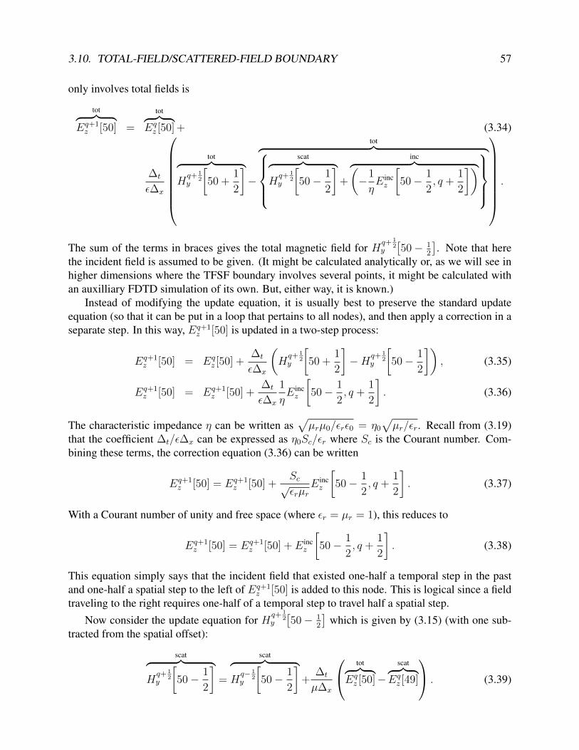
3.10. TOTAL-FIELD/SCATTERED-FIELD BOUNDARY 57
only involves total fields is
tot︷ ︸︸ ︷Eq+1z [50] =
tot︷ ︸︸ ︷Eqz [50] + (3.34)
∆t
ε∆x
tot︷ ︸︸ ︷
Hq+ 1
2y
[50 +
1
2
]−
tot︷ ︸︸ ︷scat︷ ︸︸ ︷
Hq+ 1
2y
[50− 1
2
]+
inc︷ ︸︸ ︷(−1
ηE incz
[50− 1
2, q +
1
2
])
.
The sum of the terms in braces gives the total magnetic field for Hq+ 1
2y
[50− 1
2
]. Note that here
the incident field is assumed to be given. (It might be calculated analytically or, as we will see inhigher dimensions where the TFSF boundary involves several points, it might be calculated withan auxilliary FDTD simulation of its own. But, either way, it is known.)
Instead of modifying the update equation, it is usually best to preserve the standard updateequation (so that it can be put in a loop that pertains to all nodes), and then apply a correction in aseparate step. In this way, Eq+1
z [50] is updated in a two-step process:
Eq+1z [50] = Eq
z [50] +∆t
ε∆x
(Hq+ 1
2y
[50 +
1
2
]−Hq+ 1
2y
[50− 1
2
]), (3.35)
Eq+1z [50] = Eq+1
z [50] +∆t
ε∆x
1
ηE incz
[50− 1
2, q +
1
2
]. (3.36)
The characteristic impedance η can be written as√µrµ0/εrε0 = η0
√µr/εr. Recall from (3.19)
that the coefficient ∆t/ε∆x can be expressed as η0Sc/εr where Sc is the Courant number. Com-bining these terms, the correction equation (3.36) can be written
Eq+1z [50] = Eq+1
z [50] +Sc√εrµr
E incz
[50− 1
2, q +
1
2
]. (3.37)
With a Courant number of unity and free space (where εr = µr = 1), this reduces to
Eq+1z [50] = Eq+1
z [50] + E incz
[50− 1
2, q +
1
2
]. (3.38)
This equation simply says that the incident field that existed one-half a temporal step in the pastand one-half a spatial step to the left of Eq+1
z [50] is added to this node. This is logical since a fieldtraveling to the right requires one-half of a temporal step to travel half a spatial step.
Now consider the update equation for Hq+ 1
2y
[50− 1
2
]which is given by (3.15) (with one sub-
tracted from the spatial offset):
scat︷ ︸︸ ︷Hq+ 1
2y
[50− 1
2
]=
scat︷ ︸︸ ︷Hq− 1
2y
[50− 1
2
]+
∆t
µ∆x
tot︷ ︸︸ ︷Eqz [50]−
scat︷ ︸︸ ︷Eqz [49]
. (3.39)

58 CHAPTER 3. INTRODUCTION TO THE FDTD METHOD
As was true for the update of the electric field adjacent to the TFSF boundary, this is not a consistentequation since the terms are scattered-field quantities except for Eq
z [50] which is in the total-fieldregion. To correct this, the incident field could be subtracted from Eq
z [50]. Rather than modifying(3.39), we choose to give the necessary correction as a separate equation. The correction would be
Hq+ 1
2y
[50− 1
2
]= H
q+ 12
y
[50− 1
2
]− ∆t
µ∆x
E incz [50, q]. (3.40)
With a Courant number of unity and free space, this equation becomes
Hq+ 1
2y
[50− 1
2
]= H
q+ 12
y
[50− 1
2
]− 1
η0
E incz [50, q]. (3.41)
As mentioned previously, there is nothing that requires the origin to be assigned to one par-ticular node in the grid. There is no reason that one has to associate the location x = 0 with theleft end of the grid. In the TFSF formulation it is usually most convenient to fix the origin relativeto the TFSF boundary itself. Let the origin x = 0 correspond to the node Ez[50]. Such a shiftrequires that 50 be subtracted from the spatial indices given previously for the incident field. Thecorrection equations thus become
Hq+ 1
2y
[50− 1
2
]= H
q+ 12
y
[50− 1
2
]− 1
η0
E incz [0, q], (3.42)
Eq+1z [50] = Eq+1
z [50] + E incz
[−1
2, q +
1
2
]. (3.43)
To implement a TFSF boundary, one merely has to translate (3.42) and (3.43) into the necessarystatements. A program that implements a TFSF boundary between hy[49] and ez[50] is shownin Program 3.5.
Program 3.5 1Dtfsf.c: One-dimensional simulation with a TFSF boundary between hy[49]and ez[50].
1 /* 1D FDTD simulation with a simple absorbing boundary condition2 * and a TFSF boundary between hy[49] and ez[50]. */3
4 #include <stdio.h>5 #include <math.h>6
7 #define SIZE 2008
9 int main()10 11 double ez[SIZE] = 0., hy[SIZE] = 0., imp0 = 377.0;12 int qTime, maxTime = 450, mm;13
14 char basename[80]="sim", filename[100];

3.10. TOTAL-FIELD/SCATTERED-FIELD BOUNDARY 59
15 int frame = 0;16 FILE *snapshot;17
18 /* do time stepping */19 for (qTime = 0; qTime < maxTime; qTime++) 20
21 /* simple ABC for hy[size - 1] */22 hy[SIZE - 1] = hy[SIZE - 2];23
24 /* update magnetic field */25 for (mm = 0; mm < SIZE - 1; mm++)26 hy[mm] = hy[mm] + (ez[mm + 1] - ez[mm]) / imp0;27
28 /* correction for Hy adjacent to TFSF boundary */29 hy[49] -= exp(-(qTime - 30.) * (qTime - 30.) / 100.) / imp0;30
31 /* simple ABC for ez[0] */32 ez[0] = ez[1];33
34 /* update electric field */35 for (mm = 1; mm<SIZE; mm++)36 ez[mm] = ez[mm] + (hy[mm] - hy[mm - 1]) * imp0;37
38 /* correction for Ez adjacent to TFSF boundary */39 ez[50] += exp(-(qTime + 0.5 - (-0.5) - 30.) *40 (qTime + 0.5 - (-0.5) - 30.) / 100.);41
42 /* write snapshot if time a multiple of 10 */43 if (qTime % 10 == 0) 44 sprintf(filename, "%s.%d", basename, frame++);45 snapshot = fopen(filename, "w");46 for (mm = 0; mm < SIZE; mm++)47 fprintf(snapshot, "%g\n", ez[mm]);48 fclose(snapshot);49 50 /* end of time-stepping */51
52 return 0;53
Note that this is similar to Program 3.4. Other than the incorporation of the ABC’s in line 22 and32, the only differences are the removal of the additive source (line 29 of Program 3.4) and theaddition of the two correction equations in lines 29 and 39. The added code is shown in bold. Inline 39, the half-step forward in time is obtained with qTime+0.5. The half-step back in space isobtained with the -0.5 which is enclosed in parentheses.
The waterfall plot of the fields generated by Program 3.5 is shown in Fig. 3.12. Note that the

60 CHAPTER 3. INTRODUCTION TO THE FDTD METHOD
0 20 40 60 80 100 120 140 160 180 2000
5
10
15
20
25
30
35
40
45
Space [spatial index]
Tim
e [
fra
me
nu
mb
er]
Figure 3.12: Waterfall plot of the electric fields produced by Program 3.5 which has a TFSFboundary between nodes hy[49] and ez[50].
field appears at node 50 and travels exclusively to the right—no field propagates to the left fromthe TFSF boundary. Since there is nothing to scatter the incident field in this simulation, Fig. 3.12shows only the incident field. The next step is, thus, the inclusion of some inhomogeneity in thegrid to generate scattered fields.
3.11 InhomogeneitiesThe FDTD update equations were obtained from approximations of Faraday’s and Ampere’s lawswhich were themselves differential equations. Differential equations pertain at a point. Thus, the εand µ which appear in these equations are the ones which exist at the location of the correspondingnode. It is certainly permissible that these values change from point to point. In fact, it is requiredthat they change when modeling inhomogeneous material.
Recall, from (3.19), that the electric-field update equation had a coefficient of η0Sc/εr. Assum-ing that the Courant number Sc is still unity, but allowing the relative permittivity to be a functionof position, the update equation could be implemented with a statement such as
ez[m] = ez[m] + (hy[m] - hy[m-1])*imp0/epsR[m];
where the array element epsR[m] contains the relative permittivity at the point m∆x, i.e., at apoint collocated with the node ez[m]. The size of the epsR array would be the same size as theelectric-field array and the elements have to be initialized to appropriate values.

3.11. INHOMOGENEITIES 61
The same concept applies to the relative permeability in the updating of the magnetic fieldswhere the update coefficient is given by Sc/µrη0 (ref. (3.20)). The relative permeability that existsat the point in space corresponding to the location of a particular magnetic-field node is the onethat should be used in the update equation for that node. Assuming an array muR has been createdand initialized with the values of the relative permeability, the magnetic-fields would be updatedwith an equation such as
hy[m] = hy[m] + (ez[m + 1] - ez[m]) / imp0 / muR[m];
A program that models a region of space near the interface between free space and a dielectricwith a relative permittivity of nine is shown in Program 3.6 (the permeability is that of free space).The incident field is still introduced via a TFSF boundary, which is in the free-space side of thecomputational domain, and the ABC on the left hand side is the same as before. However, thereare some other minor changes between this program and the program in Program 3.5. The electricand magnetic fields are no longer initialized when they are declared. Instead, two loops are usedto set the initial fields to zero. The magnetic field is now declared to have one fewer node than theelectric field. This was done so that the computational domain begins and ends on an electric-fieldnode. (There are no truly compelling reasons to have the computational domain begin and end withthe same field type, but such symmetry can simplify coding and some aspects of certain problems.)Because the grid now terminates on an electric field, the ABC at the right end of the grid must beapplied to this terminal electric-field node. This is accomplished with the statement in line 45.
Program 3.6 1Ddielectric.c: One-dimensional FDTD program to model an interface be-tween free-space and a dielectric that has a relative permittivity εr of 9.
1 /* 1D FDTD simulation with a simple absorbing boundary2 * condition, a TFSF boundary between hy[49] and ez[50], and3 * a dielectric material starting at ez[100] */4
5 #include <stdio.h>6 #include <math.h>7
8 #define SIZE 2009
10 int main()11 12 double ez[SIZE], hy[SIZE - 1], epsR[SIZE], imp0 = 377.0;13 int qTime, maxTime = 450, mm;14 char basename[80] = "sim", filename[100];15 int frame = 0;16 FILE *snapshot;17
18 /* initialize electric field */19 for (mm = 0; mm < SIZE; mm++)20 ez[mm] = 0.0;21

62 CHAPTER 3. INTRODUCTION TO THE FDTD METHOD
22 /* initialize magnetic field */23 for (mm = 0; mm < SIZE - 1; mm++)24 hy[mm] = 0.0;25
26 /* set relative permittivity */27 for (mm = 0; mm < SIZE; mm++)28 if (mm < 100)29 epsR[mm] = 1.0;30 else31 epsR[mm] = 9.0;32
33 /* do time stepping */34 for (qTime = 0; qTime < maxTime; qTime++) 35
36 /* update magnetic field */37 for (mm = 0; mm<SIZE - 1; mm++)38 hy[mm] = hy[mm] + (ez[mm + 1] - ez[mm]) / imp0;39
40 /* correction for Hy adjacent to TFSF boundary */41 hy[49] -= exp(-(qTime - 30.) * (qTime - 30.) / 100.) / imp0;42
43 /* simple ABC for ez[0] and ez[SIZE - 1] */44 ez[0] = ez[1];45 ez[SIZE-1] = ez[SIZE-2];46
47 /* update electric field */48 for (mm = 1; mm < SIZE - 1; mm++)49 ez[mm] = ez[mm] + (hy[mm] - hy[mm - 1]) * imp0 / epsR[mm];50
51 /* correction for Ez adjacent to TFSF boundary */52 ez[50] += exp(-(qTime + 0.5 - (-0.5) - 30.)*53 (qTime + 0.5 - (-0.5) - 30.) / 100.);54
55 /* write snapshot if time a multiple of 10 */56 if (qTime % 10 == 0) 57 sprintf(filename, "%s.%d", basename, frame++);58 snapshot = fopen(filename, "w");59 for (mm = 0; mm < SIZE; mm++)60 fprintf(snapshot, "%g\n", ez[mm]);61 fclose(snapshot);62 63 /* end of time-stepping */64
65 return 0;66
The relative-permittivity array epsR is initialize in the loop starting at line 27. If the spatial

3.11. INHOMOGENEITIES 63
0 20 40 60 80 100 120 140 160 180 2000
5
10
15
20
25
30
35
40
45
Space [spatial index]
Tim
e [
fra
me
nu
mb
er]
Figure 3.13: Waterfall plot of the electric fields produced by Program 3.6 which has a dielectricwith a relative permittivity of 9 starting at node 100. Free space is to the left of that.
index mm is less than 100, the relative permittivity is set to unity (i.e., free space), otherwise it is setto 9. The characteristic impedance of free space is η0 while the impedance for the dielectric is η0/3.Note that the update equations do not directly incorporate the dielectric impedance. Rather, the co-efficient that appears in the equation uses the impedance of free space and the relative permittivitythat pertains at that point.
When a wave is normally incident from a medium with a characteristic impedance η1 to amedium with a characteristic impedance η2, the reflection coefficient Γ and the transmission coef-ficient T are given by
Γ =η2 − η1
η2 + η1
, (3.44)
T =2η2
η2 + η1
. (3.45)
Therefore the reflection and transmission coefficients that pertain to this example are
Γ =η0/3− η0
η0/3 + η0
= −1
2, (3.46)
T =2η0/3
η0/3 + η0
=1
2. (3.47)
The waterfall plot of the data produced by Program 3.6 is shown in Fig. 3.13. Once the fieldencounters the interface at node 100, a reflected field (i.e., a scattered field) is created. Although

64 CHAPTER 3. INTRODUCTION TO THE FDTD METHOD
-0.5
-0.25
0
0.25
0.5
0 25 50 75 100 125 150 175 200
Ez (
V/m
)
Spatial Step
Time-step 100Time-step 140
Figure 3.14: Two of the snapshots produced by Program 3.6. The vertical line at node 100 corre-sponds to the interface between free space and the dielectric. The incident pulse had unit amplitude.Shown in this figure are the transmitted field (to the right of the interface) and the reflected field(to the left).
one cannot easily judge scales from the waterfall plot, it can be seen that the reflected field isnegative and appears to have about half the magnitude of the incident pulse (the peak of the incidentfield spans a vertical space corresponding to nearly two frames while the peak of the reflected fieldspans about one frame). Similarly, the transmitted pulse is positive and appears to have half themagnitude of the incident field. One can see this more clearly in Fig. 3.14 which shows the field attime-steps 100 and 140. The incident pulse had unit amplitude. At the time-steps shown here, thefield has split into the transmitted and reflected pulses, each of which has an magnitude of one-half.
Returning to the waterfall plot of Fig. 3.13, one can also see that the pulse in the dielectrictravels more slowly than the pulse in free space. With a relative permittivity of 9, the speed of lightshould be one-third of that in free space. Thus, from frame to frame the peak in the dielectric hasmoved one-third of the distance that the peak moves in free space.
There are two numerical artifacts present in Fig. 3.13, one which we need to fix and the otherwe need to understand. Note that when the reflected field encounters the left boundary it disap-pears. The ABC does its job and the field is absorbed. On the other hand, when the transmittedwave encounters the right boundary, at approximately frame 37, it is not completely absorbed. Areflected wave is produced which is visible in the upper right-hand corner of Fig. 3.13. Why isthe ABC no longer working? The problem is that the simple ABC used so far is based on the as-sumption that the wave travels one spatial step for every time step. In this dielectric, with a relativepermittivity of 9, the speed of light is one-third that of free space and hence the wave does nottravel one spatial step per time step—it travels a third of a spatial step. A possible fix might be to

3.11. INHOMOGENEITIES 65
update the electric field on the boundary with the value of the neighboring electric-field node fromthree time steps in the past. However, what if the relative permittivity of the dielectric were 2? Inthat case the speed of light would be 1/
√2 times that of free space. There would be no past value
of an interior node that could be used directly to update the boundary node. So, it is necessary torethink the implementation of the ABC so that it can handle these sorts of situations. This will beaddressed in another chapter.
The other artifact present in Fig. 3.13 is slightly less obvious. If you look at the trailing edgeof the transmitted pulse around frame 33, or so, you will see a slight wiggle. The incident fieldis a Gaussian pulse which asymptotically goes to zero to either side of the peak value. However,the transmitted pulse does not behave this way—at least not after propagating in the dielectric fora while (initially there are no wiggles visible at the trailing edge of the transmitted pulse). Thesewiggles are caused by dispersion in the FDTD grid. When the Courant number is anything otherthan unity, the FDTD grid is dispersive, meaning that different frequencies propagate at differentspeeds. Note that we have defined the Courant number as the c∆t/∆x where c is the speed of lightin free space. We will generally maintain the convention that c represents the speed of light infree space. However, one can think of the Courant number as a local quantity that equals the localspeed of light multiplied by the ratio ∆t/∆x. Because the speed of light is one-third of that of freespace, the local Courant number in the dielectric is not unity. Since the Gaussian pulse consists ofa range of frequencies, and these frequencies are propagating at different speeds, the pulse “breaksapart” as it propagates. In practice, one tries to ensure that the amount of dispersion is small, but itis unavoidable in multi-dimensional FDTD analysis. Dispersion will be considered further later.
Because of the discretized nature of the FDTD grid, the location of a material boundary canbe somewhat ambiguous. The relatively permittivity that pertains to a particular electric-field nodecan be assumed to exist over the space that extends from one of its neighboring magnetic-fieldnodes to the other neighboring magnetic-field node. This idea is illustrated in Fig. 3.15 whichshows a portion of the FDTD grid together with the permittivity associated with each node. Thepermittivities are indicated with the bar along the bottom of the figure.
If there is only a change in permittivity, the location of the interface between the different mediaseems rather clear. It coincides with the magnetic-field node that has ε1 to one side and ε2 to theother. However, what if there is a change in permeability too? The permeabilities are indicatedwith a bar along the top of the figure. It is seen that the interface associated with the change inpermeabilities is not aligned with the interface associated with the change in permittivities. Oneway to address this problem is to assume the true interface is aligned with an electric-field node.This node would then use the average of the permittivities of the media to either side. This scenariois depicted in Fig. 3.16. Alternatively, if one wants to have the boundary aligned with a magnetic-field node, then the node located on the boundary would use the average of the permeabilities toeither side while the electric-field nodes would use the permittivity of the first medium if they wereto the left of the boundary and use the permittivity of the second medium if they were to the right.

66 CHAPTER 3. INTRODUCTION TO THE FDTD METHOD
Ez
Hy Hy Hy HyHy
EzEzEzEz
ε1 ε1 ε2 ε2
µ1 µ2µ1 µ2µ1
ε2
Hy
Ez
position, x
Figure 3.15: One-dimensional grid depicting an abrupt change in both the permittivity and perme-ability. The actual location of the interface between the two media is ambiguous.
Ez
Hy Hy Hy HyHy
EzEzEzEz
ε1 ε1 ε2 ε2
µ1 µ2µ1 µ2µ1
εavg
Hy
Ez
position, x
Figure 3.16: One-dimensional grid depicting a change from one medium to another. An electric-field node is assumed to be collocated with the interface, hence the permittivity used there is theaverage of the permittivities to either side.
3.12 Lossy MaterialWhen a material has a finite conductivity σ, a conduction-current term is added to Ampere’s law(which is distinct from the source-current term mentioned in Sec. 3.8). Thus,
σE + ε∂E
∂t= ∇×H. (3.48)
The discretized form of Ampere’s law provided the update equation for the electric field. As before,assuming only a z component of the field and variation only in the x direction, this equation reducesto
σEz + ε∂Ez∂t
=∂Hy
∂x. (3.49)
As discussed in Sec. 3.3 and detailed in Fig. 3.2, this equation was expanded about the point(m∆x, (q + 1/2)∆t) to obtain the electric-field update equation. However, when loss is present,the undifferentiated electric field appears on the left side of the equation. With the assumedarrangement of the nodes shown in Fig. 3.2, there is no electric field at the space-time point(m∆x, (q + 1/2)∆t). This problem can be circumvented by using the averaging (in time) of theelectric field to either side of the desired point, i.e.,
Eq+ 1
2z [m] ≈ Eq+1
z [m] + Eqz [m]
2. (3.50)
Thus a suitable discretization of Ampere’s law when loss is present is
σEq+1z [m] + Eq
z [m]
2+ ε
Eq+1z [m]− Eq
z [m]
∆t
=Hq+ 1
2y
[m+ 1
2
]−Hq+ 1
2y
[m− 1
2
]∆x
. (3.51)

3.12. LOSSY MATERIAL 67
As before, this can be solved forEq+1z [m], which is the “future” field, in terms of purely past fields.
The result is
Eq+1z [m] =
1− σ∆t
2ε
1 + σ∆t
2ε
Eqz [m] +
∆t
ε∆x
1 + σ∆t
2ε
(Hq+ 1
2y
[m+
1
2
]−Hq+ 1
2y
[m− 1
2
]). (3.52)
When σ is zero this reduces to the previous update equation (3.18).In previous update equations it was possible to express the coefficients in terms of the Courant
number, i.e., the ratio of the temporal step to the spatial step. In (3.52) it appears the term σ∆t/2εrequires that the temporal step be specified (together with the conductivity and permittivity). How-ever, there is a way to express this such that the temporal step does not need to be stated explicitly.This will be considered in detail in Sec. 5.7.
As we will see, it is occasionally helpful to incorporate a magnetic conduction current in Fara-day’s law. Similar to the electric conduction current, the magnetic conduction current is assumedto be the product of the magnetic conductivity σm and the magnetic field. Faraday’s law becomes
−σmH− µ∂H
∂t= ∇× E. (3.53)
We again restrict consideration to an Hy component which varies only in the x direction. Thisreduces to
σmHy + µ∂Hy
∂t=∂Ez∂x
. (3.54)
As before, this is expanded/discretized at the space-time point ((m + 1/2)∆x, q∆t). Since thereis no magnetic field available at integer time steps, the magnetic field is averaged in time to get anapproximation of the field at time q∆t. This yields
σmHq+ 1
2y
[m+ 1
2
]+H
q− 12
y
[m+ 1
2
]2
+ µHq+ 1
2y
[m+ 1
2
]−Hq− 1
2y
[m+ 1
2
]∆t
=
Eqz [m+ 1]− Eq
z [m]
∆x
. (3.55)
Solving for Hq+ 1
2y
[m+ 1
2
]yields the update equation
Hq+ 1
2y
[m+
1
2
]=
1− σm∆t
2µ
1 + σm∆t
2µ
Hq− 1
2y
[m+
1
2
]+
∆t
µ∆x
1 + σm∆t
2µ
(Eqz [m+ 1]− Eq
z [m]) . (3.56)
When σm is zero this reduces to (3.15).Program 3.7 models a lossy dielectric half-space that starts at node 100. As before, the relative
permittivity is 9. However there is also an electric loss present such that σ∆t/2ε is 0.01. Theprogram uses two coefficient arrays, ceze and cezh. The terms in the ceze array multiplythe previous (or “self”) term while the cezh array contains the terms that multiply the spatialdifference of the magnetic fields. Think of these arrays as consisting of coefficients (or constants),hence the “c” at the start of their name, that appear in the Ez update equation, hence the ez partof the name, and multiplying either the electric field (ceze) or the magnetic field (cezh). Thevalues of these arrays are set in the loop that starts at line 27. Since the simple ABC previously

68 CHAPTER 3. INTRODUCTION TO THE FDTD METHOD
employed at the right edge of the grid does not work, it has been removed but the left side of thegrid is terminated as before. The magnetic field update is unchanged from before. A waterfall plotof the data produced by Program 3.7 is shown in Fig. 3.17. The pulse decays as it propagates inthe lossy region and eventually decays to a rather negligible value. Thus the lack of an ABC at theright side of the grid is not really a concern in this particular instance.
Program 3.7 1Dlossy.c: One-dimensional simulation with a lossy dielectric region.
1 /* 1D FDTD simulation of a lossy dielectric region. */2
3 #include <stdio.h>4 #include <math.h>5
6 #define SIZE 2007 #define LOSS 0.018
9 int main()10 11 double ez[SIZE], hy[SIZE - 1], ceze[SIZE], cezh[SIZE],12 imp0 = 377.0;13 int qTime, maxTime = 450, mm;14 char basename[80] = "sim", filename[100];15 int frame = 0;16 FILE *snapshot;17
18 /* initialize electric field */19 for (mm = 0; mm < SIZE; mm++)20 ez[mm] = 0.0;21
22 /* initialize magnetic field */23 for (mm = 0; mm < SIZE - 1; mm++)24 hy[mm] = 0.0;25
26 /* set electric-field update coefficients */27 for (mm = 0; mm < SIZE; mm++)28 if (mm < 100) /* free space */29 ceze[mm] = 1.0;30 cezh[mm] = imp0;31 else /* lossy dielectric */32 ceze[mm] = (1.0 - LOSS) / (1.0 + LOSS);33 cezh[mm] = imp0 / 9.0 / (1.0 + LOSS);34 35
36 /* do time stepping */37 for (qTime = 0; qTime < maxTime; qTime++) 38

3.12. LOSSY MATERIAL 69
39 /* update magnetic field */40 for (mm = 0; mm < SIZE - 1; mm++)41 hy[mm] = hy[mm] + (ez[mm + 1] - ez[mm]) / imp0;42
43 /* correction for Hy adjacent to TFSF boundary */44 hy[49] -= exp(-(qTime - 30.) * (qTime - 30.) / 100.) / imp0;45
46 /* simple ABC for ez[0] */47 ez[0] = ez[1];48
49 /* update electric field */50 for (mm = 1; mm < SIZE - 1; mm++)51 ez[mm] = ceze[mm] * ez[mm] + cezh[mm] * (hy[mm] - hy[mm - 1]);52
53 /* correction for Ez adjacent to TFSF boundary */54 ez[50] += exp(-(qTime + 0.5 - (-0.5) - 30.) *55 (qTime + 0.5 - (-0.5) - 30.) / 100.);56
57 /* write snapshot if time a multiple of 10 */58 if (qTime % 10 == 0) 59 sprintf(filename, "%s.%d", basename, frame++);60 snapshot=fopen(filename, "w");61 for (mm = 0; mm < SIZE; mm++)62 fprintf(snapshot, "%g\n", ez[mm]);63 fclose(snapshot);64 65 /* end of time-stepping */66
67 return 0;68
When loss is present the characteristic impedance of the medium becomes
η =
√√√√µ(
1− j σmωµ
)ε(1− j σ
ωε
) = η0
√√√√µr
(1− j σm
ωµ
)εr(1− j σ
ωε
) (3.57)
When σm/µ = σ/ε the terms in parentheses are equal and hence cancel. With those terms canceled,the characteristic impedance is indistinguishable from the lossless case. Therefore
η|σmµ
=σε
= η|σm=σ=0 = η0
√µrεr. (3.58)
As shown in (3.44), the reflection coefficient for a wave normally incident on a planar boundaryis proportional to the difference of the impedances to either side of the interface. If the materialon one side is lossless while the material on the other side is lossy with σm/µ = σ/ε, then theimpedances are matched provided the ratios of εr and µr are also matched across the boundary.

70 CHAPTER 3. INTRODUCTION TO THE FDTD METHOD
0 20 40 60 80 100 120 140 160 180 2000
5
10
15
20
25
30
35
40
45
Space [spatial index]
Tim
e [
fra
me
nu
mb
er]
Figure 3.17: Waterfall plot of the electric fields produced by Program 3.7 which has a lossy dielec-tric region with a relative permittivity of 9 starting at node 100.
With the impedances matched, there will be no reflection from the interface. Therefore a lossylayer could be used to terminate the grid. The fields will dissipate in this lossy region and, if theregion is large enough, may be small by the time they encounter the end of the grid. Upon reflectionfrom the end of the grid, the fields would have to propagate back through the lossy layer where theywould decay even further. With proper design the reflected fields can be made inconsequentiallysmall when they eventually get back to the lossless portion of the grid.
A lossy layer with the impedance matched to the previous region can be implemented easily inone dimension. Program 3.8 shows a program where a lossless dielectric layer with εr = 9 startsat node 100. The lossless region extends to node 180. At node 180, and beyond, the material hasboth a nonzero electric and a magnetic conductivity. The conductivities are matched in the sensethat σm/µ = σ/ε. Thus the terms σm∆t/2µ and σ∆t/2ε in the update-equations are also matched.In this program these terms are set to 0.02. The coefficients used in the magnetic-field updateequations are stored in the arrays chyh and chye.
The waterfall plot of the data generated by Program 3.8 is shown in Fig. 3.18. The fieldsthat enter the lossless region propagate to the right and eventually encounter the lossy region.Because the impedances of the lossless and lossy media are matched, the fields enter the lossyregion without reflection (actually, that is true in the continuous world, but only approximately truein the discretized FDTD world—there is some small reflection present). As the fields propagate inthe lossy region they dissipate to the point where they are almost negligible when they reenter thelossless region. There is no reflected field evident in the upper right corner of the plot.

3.12. LOSSY MATERIAL 71
Program 3.8 1Dmatched.c: Program with a lossless dielectric region followed by a lossy layerthat has its impedance matched to the lossless dielectric.
1 /* 1D FDTD simulation of a lossless dielectric region2 * followed by a lossy layer which matches the impedance3 * of the dielectric. */4
5 #include <stdio.h>6 #include <math.h>7
8 #define SIZE 2009 #define LOSS 0.02
10 #define LOSS_LAYER 18011
12 int main()13 14 double ez[SIZE], hy[SIZE - 1], ceze[SIZE], cezh[SIZE],15 chyh[SIZE - 1], chye[SIZE - 1], imp0 = 377.0;16 int qTime, maxTime = 450, mm;17 char basename[80] = "sim", filename[100];18 int frame = 0;19 FILE *snapshot;20
21 /* initialize electric field */22 for (mm = 0; mm < SIZE; mm++)23 ez[mm] = 0.0;24
25 /* initialize magnetic field */26 for (mm = 0; mm < SIZE - 1; mm++)27 hy[mm] = 0.0;28
29 /* set electric-field update coefficients */30 for (mm = 0; mm < SIZE; mm++)31 if (mm < 100) 32 ceze[mm] = 1.0;33 cezh[mm] = imp0;34 else if (mm < LOSS_LAYER) 35 ceze[mm] = 1.0;36 cezh[mm] = imp0 / 9.0;37 else 38 ceze[mm] = (1.0 - LOSS) / (1.0 + LOSS);39 cezh[mm] = imp0 / 9.0 / (1.0 + LOSS);40 41
42 /* set magnetic-field update coefficients */43 for (mm = 0; mm < SIZE - 1; mm++)44 if (mm < LOSS_LAYER)

72 CHAPTER 3. INTRODUCTION TO THE FDTD METHOD
45 chyh[mm] = 1.0;46 chye[mm] = 1.0 / imp0;47 else 48 chyh[mm] = (1.0 - LOSS) / (1.0 + LOSS);49 chye[mm] = 1.0 / imp0 / (1.0 + LOSS);50 51
52 /* do time stepping */53 for (qTime = 0; qTime < maxTime; qTime++) 54
55 /* update magnetic field */56 for (mm = 0; mm < SIZE - 1; mm++)57 hy[mm] = chyh[mm] * hy[mm] +58 chye[mm] * (ez[mm + 1] - ez[mm]);59
60 /* correction for Hy adjacent to TFSF boundary */61 hy[49] -= exp(-(qTime - 30.) * (qTime - 30.) / 100.) / imp0;62
63 /* simple ABC for ez[0] */64 ez[0] = ez[1];65
66 /* update electric field */67 for (mm = 1; mm < SIZE - 1; mm++)68 ez[mm] = ceze[mm] * ez[mm] +69 cezh[mm] * (hy[mm] - hy[mm - 1]);70
71 /* correction for Ez adjacent to TFSF boundary */72 ez[50] += exp(-(qTime + 0.5 - (-0.5) - 30.)*73 (qTime + 0.5 - (-0.5) - 30.) / 100.);74
75 /* write snapshot if time a multiple of 10 */76 if (qTime % 10 == 0) 77 sprintf(filename, "%s.%d", basename, frame++);78 snapshot=fopen(filename, "w");79 for (mm = 0; mm < SIZE; mm++)80 fprintf(snapshot, "%g\n", ez[mm]);81 fclose(snapshot);82 83 /* end of time-stepping */84
85 return 0;86

3.12. LOSSY MATERIAL 73
0 20 40 60 80 100 120 140 160 180 2000
5
10
15
20
25
30
35
40
45
Space [spatial index]
Tim
e [
fra
me
nu
mb
er]
Figure 3.18: Waterfall plot of the electric fields produced by Program 3.8 which has a dielectricregion starting at node 100 with a relative permittivity of 9. This lossless region is followed by alossy layer with matched impedance. The lossy region starts at node 180.

74 CHAPTER 3. INTRODUCTION TO THE FDTD METHOD

Chapter 4
Improving the FDTD Code
4.1 IntroductionThe C code presented in the previous chapter adequately served its purpose—it implemented thedesired FDTD functionality in a relatively straightforward way. However, as the algorithms getmore involved, for instance, when implementing simulations of two- or three-dimensional prob-lems, the readability, portability, and maintainability will be improved if our implementation isslightly more sophisticated. In this chapter we will implement the algorithms of the previous chap-ter in a way which may seem, at first, to be overly complicated. However, as the complexity ofthe algorithms increases in coming chapters, we will see that the effort required to understand thismore sophisticated approach will have been worth it.
4.2 Arrays and Dynamic Memory AllocationIn C an array is stored in a block of contiguous memory. Memory itself is fundamentally a one-dimensional quantity since memory is ultimately accessed with a single memory address. Let usconsider a one-dimensional array of doubles ez where the size is specified at run-time rather thanat compile-time. The compiler needs to know about the existence of this array, but at compile-timeit does not need to know the amount or the location of memory where the array will be stored. Wecan specify the size of the array when the program is run and we can allow the computer to decidethe location of the necessary amount of memory. The compiler is told about the potential existenceof the array with a pointer. Once the pointer is associated with the appropriate block of memory, itis virtually indistinguishable from a one-dimensional array.
The code shown in Fragment 4.1 demonstrates how the array ez can be created at run-time.In line 1 ez is declared as a pointer—it can store an address but when the program initially startsit does not point to anything meaningful. Line 2 declares two integer variables: num elementswhich will contain the number of elements in the array, and mm which will be used as a loopcounter. Lines 4 and 5 determine the number of elements the user desires.
Lecture notes by John Schneider. fdtd-improved-code.tex
75

76 CHAPTER 4. IMPROVING THE FDTD CODE
Fragment 4.1 Fragment of code demonstrating how the size of the array ez can be set at run-time. The header file stdlib.h would typically have to be included to provide the prototype forthe calloc() function.
1 double *ez;2 int num_elements, mm;3
4 printf("Enter the size of the array: ");5 scanf("%d", &num_elements);6
7 ez = calloc(num_elements, sizeof(double));8
9 for (mm=0; mm < num_elements; mm++)10 ez[mm] = 3.0 * mm;
Line 7 is the key to getting ez to behave as an array. In this line the pointer ez is set equal to thememory address that is returned by the function calloc().∗ calloc() takes two arguments.The first specifies the number of elements in the array while the second specifies the amount ofmemory needed for a single element. Here the sizeof() operator is used to obtain the size ofa double variable. (Although not shown in this fragment, when using the calloc() functionone typically has to include the header file stdlib.h to provide the function prototype.) Ifcalloc() is unable to provide the requested memory it will return NULL. †
After the call of calloc() in line 7, ez points to the start of a contiguous block of memorywhere the array elements can be stored. To demonstrate this, lines 9 and 10 write the value of threetimes the array index to each element of the array (so that ez[0] would be 0.0, ez[1] would be3.0, ez[2] would be 6.0, and so on).
Some compilers will actually complain about the code as it is written in Fragment 4.1. The“problem” is that technically calloc() returns a void pointer—it is simply the address of thestart of a block of memory, but we have not said what is stored at that memory. We want a pointerto doubles since we will be storing double precision variables in this memory. The compilerreally already knows this since we are storing the address in ez which is a pointer to doubles.Nevertheless, some compilers will give a warning because of line 7. Therefore, to ensure thatcompilers do not complain, it would be best to replace line 7 with
ez = (double *)calloc(num_elements, sizeof(double));
In this way the void pointer returned by calloc() is converted (or cast) to a pointer to doubles.
∗calloc() is closely related to the function malloc() which also allocates a block of memory and returnsthe address of the start of that block. However calloc() returns memory which has been cleared, i.e., set to zero,while malloc() returns memory which may contain anything. Since we want the field arrays initially to be zero, itis better to use calloc() than malloc().†Robust code would check the return value and take appropriate measures if NULL were returned. For now we will
assume that calloc() succeeded.

4.3. MACROS 77
4.3 MacrosC provides a preprocessor which “processes” your code prior to the compiler itself. Preprocessordirectives start with the pound sign (#) and instruct the preprocessor to do things such as includea header file (with an #include statement) or substitute one string for another. Program 3.1 hadthree preprocessor directives. Two were used to include the files stdio.h and math.h and oneused a #define statement to tell the preprocessor to substitute 200 for all occurrences of thestring SIZE.
Compilers allow you to see what the source code is after passing through the preprocessor.Using the GNU C compiler, one adds the -E flag to the compiler command to obtain the outputfrom the preprocessor. So, for example, one can see the source code as it appears after passingthrough the preprocessor with the command
gcc -E 1DbareBones.c
In this case you will observe that there are many, many more lines of output than there are in youroriginal program. This is because of the inclusion of the header files. Your original program willappear at the end of the output except now SIZE does not appear anywhere. Instead, any place ithad appeared you will now see 200.
The #define statement can also be used to create a macro. Unlike the simple string substi-tution used before, a macro can take one or more arguments. These arguments dictate how stringsgiven as arguments should re-appear in the output. For example, consider the following macro
#define SQR(X) ((X) * (X))
This tells the preprocessor that every time SQR appears in the source code, the preprocessor shouldtake whatever appeared as an argument and replace that with the argument multiplied by itself.Here the argument X is just serving as a place holder. Consider the following code
a = 6.0 * SQR(3.0 + 4.0);
After passing through the preprocessor, this code would appear as
a = 6.0 * ((3.0 + 4.0) * (3.0 + 4.0));
The result would be that a would be set equal to 6× 72 = 294.It may seem that there are an excess number of parentheses in this macro, but one must be
careful with macros to ensure the desired results are obtained. Consider this macro
#define BAD_SQR(X) X * X
If a program then contained this statement
a = 6.0 * BAD_SQR(3.0 + 4.0);
the preprocessor translates this to
a = 6.0 * 3.0 + 4.0 * 3.0 + 4.0;

78 CHAPTER 4. IMPROVING THE FDTD CODE
Since multiplication has a higher precedence than addition, in this case a would be set equal to18 + 12 + 4 = 34. There is no harm in using extra parentheses, so do not hesitate to use them toensure you are getting precisely what you want.
It is also worth noting that the macro definition itself will typically not be terminated by asemicolon. If one includes a semicolon, it could easily produce unintended results. As an example,consider
#define BAD_SQR1(X) ((X) * (X));
If a program then contained this statement
a = BAD_SQR1(4.0) + 10.0;
the preprocessor would translate this to
a = ((4.0) * (4.0)); + 10;
Note that the “+ 10” is consider a separate statement since there is a semicolon between it andthe squared term.‡ Thus, a will be set to 16.0.
Macros may have any number of arguments. As an example, consider
#define FOO(X, Y) (Y) * cos((X) * (Y))
Given this macro, the following code
a = FOO(cos(2.15), 7.0 * sqrt(4.0));
would be translated by the preprocessor to
a = (7.0 * sqrt(4.0)) * cos((cos(2.15)) * (7.0 * sqrt(4.0)))
Macros can span multiple lines provided the newline character at the end of each line is“quoted” with a backslash. Said another way, a backslash must be the last character on a lineif the statement is to continue on the next line.
There is another “trick” that one can do with macros. One can say they want the string versionof an argument in the preprocessor output, essentially the argument will appear enclosed in quotesin the output. To understand why this is useful, it first helps to recall that in C, if one puts twostring next to each other, the compiler treats the two separate strings as a single string. Thus, thefollowing commands are all equivalent
printf("Hello world.\n");printf("Hello " "world.\n");printf("Hello "
"world.\n");
Each of these produce the output
Hello world.
‡When using the GNU C compiler, this “bad” code will compile without error. If one adds the -Wall flag whencompiling, the GNU compiler will provide a warning that gives the line number and a statement such as “warning:statement with no effect.” Nevertheless, the code will compile.

4.3. MACROS 79
Note that there is no comma between the separated strings in the printf() statements and theamount of whitespace between the strings is irrelevant.
If we want the preprocessor to produce the string version of an argument in the output, we affix# to the argument name in the place where it should appear in the output. For example, we coulduse a macro to print what is being calculated and show the result of the calculation as well:
#define SHOW_CALC(X) \printf(#X " = %g\n", X)
The first line of this macro is terminated with a backslash telling the preprocessor that the definitionis continued on the next line. Now, if the code contained
SHOW_CALC(6.0 + 24.0 / 8.0);
the preprocessor would convert this to
printf("6.0 + 24.0 / 8.0" " = %g\n", 6.0 + 24.0 / 8.0);
When the program is run, the following would be written to the screen
6.0 + 24.0 / 8.0 = 9
We are now at a point where we can construct a fairly sophisticated macro to do memoryallocation. The macro will check if the allocation of memory was successful. If not, the macro willreport the problem and terminate the program. The following fragment shows the desired code.
Fragment 4.2 Macro for allocating memory for a one-dimensional array. The trailing backslashesmust appear directly before the end of the line. (By “quoting” the newline character at the end ofthe line we are telling the preprocessor the definition is continued on the next line.)
1 #define ALLOC_1D(PNTR, NUM, TYPE) \2 PNTR = (TYPE *)calloc(NUM, sizeof(TYPE)); \3 if (!PNTR) \4 perror("ALLOC_1D"); \5 fprintf(stderr, \6 "Allocation failed for " #PNTR ". Terminating...\n");\7 exit(-1); \8
The macro ALLOC 1D() takes three arguments: a pointer (called PNTR), an integer specifyingthe number of elements (NUM), and a data type (TYPE). The macro uses calloc() to obtain thedesired amount of memory. It then checks if the allocation was successful. Recall that calloc()will return NULL if it failed to allocate the requested memory. In C, the exclamation mark isalso the “not operator.” So, if the value of PNTR is NULL (or, thought of another way, “false”),then !PNTR would be true. If the memory allocation failed, two error messages are printed (onemessage is generated using the system function perror(), the other uses fprintf() and

80 CHAPTER 4. IMPROVING THE FDTD CODE
writes the output to stderr, which is typically the screen). The program is then terminated withthe exit() command.
With this macro in our code we could create an array ez with 200 elements with statementssuch as
double *ez;
ALLOC_1D(ez, 200, double);
Technically the semicolon in the second statement is not necessary (since this macro translates toa block of code that ends with a close-brace), but there is no harm in having it.
4.4 StructuresIn C one can group data together, essentially create a compound data type, using what is knownas a structure. A program can have different types of structures, i.e., ones that bundle togetherdifferent kinds of data. For example, a program might use structures that bundle together a person’sage, weight, and name as well as structures that bundle together a person’s name, social securitynumber, and income. Just as we can have multiple variables of a given type and each variableis a unique instance of that data type, we can have multiple variables that corresponds to a givenstructure, each of which is a unique instance of that structure.
Initially, when declaring a structure, we first tell the compiler the composition of the structure.As an example, the following command defines a person structure that contains three elements:a character pointer called name that will be used to store the name of a person, an integer calledage that will correspond to the person’s age, and an integer called weight that will correspondto the person’s weight.
struct person char *name;int age;int weight;
;
This statement is merely a definition—no structure has been created yet. To create a personstructure called bob and another one called sue, a command such as the following could be used:
struct person bob, sue;
Actually, one could combine these two statements and create bob and sue with the following:
struct person char *name;int age;int weight;
bob, sue;
However, in the code to come, we will use a variant of the two-statement version of creatingstructures. It should also be pointed out that elements do not need to be declared with individualstatements of their own. For example, we could write

4.4. STRUCTURES 81
int age, weight;
instead of the two separate lines shown above.To access the elements of a structure we write the name of the structure, a dot, and then the
name of the element. For example, bob.age would be the age element of the structure bob,and sue.age would be the age element of the structure sue (despite the fact that these are bothage elements, they are completely independent variables).
Now, let’s write a program that creates two person structures. The program has a func-tion called showPerson1() to show the elements of a person and another function calledchangePerson1() that reduces the person’s age by two and decreases the weight by five. Eachof these functions takes a single argument, a person structure. The program is shown in Program4.3.
Program 4.3 struct-demo1.c: Program to demonstrate the basic use of structures.
1 /* Program to demonstrate the use of structures. Here structures are2 passed as arguments to functions.*/3
4 #include <stdio.h>5
6 struct person 7 char *name;8 int age;9 int weight;
10 ;11
12 void changePerson1(struct person p);13 void showPerson1(struct person p);14
15 int main() 16 struct person bob, sue;17
18 sue.name = "Sue";19 sue.age = 21;20 sue.weight = 120;21
22 bob.name = "Bob";23 bob.age = 62;24 bob.weight = 180;25
26 showPerson1(sue);27
28 printf("*** Before changePerson1() ***\n");29 showPerson1(bob);30 changePerson1(bob);31 printf("*** After changePerson1() ***\n");

82 CHAPTER 4. IMPROVING THE FDTD CODE
32 showPerson1(bob);33
34 return 0;35 36
37 /* Function to display the elements in a person. */38 void showPerson1(struct person p) 39 printf("name: %s\n", p.name);40 printf("age: %d\n", p.age);41 printf("weight: %d\n", p.weight);42 return;43 44
45 /* Function to modify the elements in a person. */46 void changePerson1(struct person p) 47 p.age = p.age - 2;48 p.weight = p.weight - 5;49 printf("*** In changePerson1() ***\n");50 showPerson1(p);51 return;52
In line 16 of the main() function we declare the two person structures bob and sue. Thisallocates the space for these structures, but as yet their elements do not have meaningful values.In 18 we set the name of element of sue. The following two lines set the age and weight.The elements for bob are set starting at line 22. In line 26 the showPerson1() function iscalled with an argument of sue. This function, which starts on line 38, shows the name, age, andweight of a person.
After showing the elements of sue, in line 29 of main(), showPerson1() is used to showthe elements of bob. In line 30 the function changePerson1() is called with an argument ofbob. This function, which is given starting on line 46, subtracts two from the age and five fromthe weight. After making these modifications, in line 50, showPerson1() is called to displaythe modified person.
Finally, returning to line 32 of the main() function, the showPerson1() function is calledonce again with an argument of bob. Note that this is after bob has supposedly been modified bythe changePerson1() function. The output produced by Program 4.3 is
name: Sueage: 21weight: 120
*** Before changePerson1() ***name: Bobage: 62weight: 180
*** In changePerson1() ***name: Bob

4.4. STRUCTURES 83
age: 60weight: 175
*** After changePerson1() ***name: Bobage: 62weight: 180
Here we see that the initial values of sue and bob are as we would anticipate. Also, whenshowPerson1() is called from within changePerson1(), we see the modified values forbob, i.e., his age has been reduced by two and his weight has been reduced by five. However,the last three lines of output show that, insofar as the bob structure in the main() function isconcerned, nothing has changed! bob has not been modified by changePerson1().
Although this behavior may not have been what we would have anticipated, it is correct. Whena structure is given as an argument, the function that is called is given a complete copy of theoriginal structure. Thus, when that function modifies the elements of the structure, it is modifyinga copy of the original—it is not affecting the original itself.
If we want a function that we call to be able to modify a structure, we must pass a pointer to thatstructure. We will modify the code to permit this but let use first introduce the typedef statementthat allows to write slightly cleaner code. Having to write struct person everywhere we wantto specify a person structure is slightly awkward. C allows us to use the typedef statement todefine an equivalent. The following statement tells the compiler that Person is the equivalent ofstruct person
typedef struct person Person;
Note that there is no requirement that we use the same word for the structure and the typedef-equivalent. Additionally, even when using the same word, there is no need to use different capital-ization (since the structure and its equivalent are maintained in different name spaces).
Now, let us assume we want to create two pointers to structures, one named susan and onerobert. These can be created with
struct person *susan, *robert;
Assuming the typedef statement given above has already appeared in the program, we couldinstead write:
Person *susan, *robert;
susan and robert are pointers to structures but, initially, they do not actually point to anystructures. We cannot set their elements because there is is no memory allocated for the storage ofthese elements. Thus, we must allocate memory for these structures and ensure the pointers pointto the memory.
To accomplish this, we can include in our program a statement such as
ALLOC_1D(susan, 1, Person);
Recalling the ALLOC 1D() macro presented in Sec. 4.3, this statement will allocate the memoryfor one Person and associate that memory with the pointer susan. We can now set the elementassociated with susan. However, accessing the elements of a pointer to a Person is differentthan directly accessing the elements of a Person. To set the age element of susan we wouldhave to write either

84 CHAPTER 4. IMPROVING THE FDTD CODE
(*susan).age = 21;
or
susan->age = 21;
Program 4.4 is similar to Program 4.3 in many respects except here, rather than using structuresdirectly, the program primarily deals with pointers to structures. As will be shown, this allows otherfunctions to change the elements within any given structure—the function merely has to be passeda pointer to the structure rather than (a copy of) the structure.
Program 4.4 struct-demo2.c: Program to demonstrate the basic use of pointers to struc-tures.
1 /* Program to demonstrate the use of pointers to structures. */2
3 #include <stdlib.h>4 #include <stdio.h>5
6 #define ALLOC_1D(PNTR, NUM, TYPE) \7 PNTR = (TYPE *)calloc(NUM, sizeof(TYPE)); \8 if (!PNTR) \9 perror("ALLOC_1D"); \
10 fprintf(stderr, \11 "Allocation failed for " #PNTR ". Terminating...\n");\12 exit(-1); \13 14
15 struct person 16 char *name;17 int age;18 int weight;19 ;20
21 typedef struct person Person;22
23 void changePerson2(Person *p);24 void showPerson2(Person *p);25
26 int main() 27 Person *robert, *susan;28
29 ALLOC_1D(susan, 1, Person);30 ALLOC_1D(robert, 1, Person);31
32 susan->name = "Susan";33 susan->age = 21;

4.4. STRUCTURES 85
34 susan->weight = 120;35
36 robert->name = "Robert";37 robert->age = 62;38 robert->weight = 180;39
40 showPerson2(susan);41
42 printf("*** Before changePerson2() ***\n");43 showPerson2(robert);44 changePerson2(robert);45 printf("*** After changePerson2() ***\n");46 showPerson2(robert);47
48 return 0;49 50
51 /* Function to display the elements in a person. */52 void showPerson2(Person *p) 53 printf("name: %s\n", p->name);54 printf("age: %d\n", p->age);55 printf("weight: %d\n", p->weight);56 return;57 58
59 /* Function to modify the elements in a person. */60 void changePerson2(Person *p) 61 p->age = p->age - 2;62 p->weight = p->weight - 5;63 printf("*** In changePerson2() ***\n");64 showPerson2(p);65 return;66
The typedef statement in line 21 allows us to write simply Person instead of struct person.This is followed by the prototypes for functions showPerson2() and changePerson2().These functions are similar to the corresponding functions in the previous program except now thearguments are pointers to structures instead of structures. Thus, the syntactic changes are necessaryin the functions themselves (e.g., we have to write p->age instead of p.age). Starting on line29 the ALLOC 1D() macro is used to allocate the memory for the susan and robert pointersthat were declared in line 27. The values of the elements are then set, the contents of the structuresdisplayed, robert is modified, and the contents or robert are shown again.
The output produced by Program 4.4 is
name: Susanage: 21

86 CHAPTER 4. IMPROVING THE FDTD CODE
weight: 120
*** Before changePerson2() ***name: Robertage: 62weight: 180
*** In changePerson2() ***name: Robertage: 60weight: 175
*** After changePerson2() ***name: Robertage: 60weight: 175
Note that in this case, the changes made by changePerson2() are persistent—when the main()function shows the elements of robert we see the modified values (unlike with the previous pro-gram).
4.5 Improvement Number OneNow let us use some of the features discussed in the previous sections in a revised version of the“bare-bones” program that appeared in Sec. 3.5. Here we will bundle much of the data associatedwith an FDTD simulation into a structure that we will call a Grid structure. (We will often referto this structure as simply the Grid or a Grid.) Here will define the Grid as follows:
struct Grid double *ez; // electric field arraydouble *hy; // magnetic field arrayint sizeX; // size of computational domainint time, maxTime; // current and max time stepdouble cdtds; // Courant number
;
In the “improved” program that we will soon see, there will not appear to be much reason forcreating this structure. Why bother? The motivation will be more clear when we start to modularizethe code so that different functions handle different aspects of the FDTD simulation. By bundlingall the relevant information about the simulation into a structure, we can simply pass as an argumentto each function a pointer to this Grid.
First, let us create a header file fdtd1.h in which we will put the definition of a Gridstructure. In this file we will also include the (1D) macro for allocating memory. Finally, in a questto keep the code as clean as possible, we will also define a few additional preprocessor directives: amacro for accessing the ez array elements, a macro for accessing the hy array elements, and somesimple #define statements to facilitate references to sizeX, time, maxTime, and cdtds.The complete header file is shown in Program 4.5.

4.5. IMPROVEMENT NUMBER ONE 87
Program 4.5 fdtd1.h: Header file for the first “improved” version of a simple 1D FDTD pro-gram.
1 #ifndef _FDTD1_H2 #define _FDTD1_H3
4 #include <stdio.h>5 #include <stdlib.h>6
7 struct Grid 8 double *ez;9 double *hy;
10 int sizeX;11 int time, maxTime;12 double cdtds;13 ;14
15 typedef struct Grid Grid;16
17 /* memory allocation macro */18 #define ALLOC_1D(PNTR, NUM, TYPE) \19 PNTR = (TYPE *)calloc(NUM, sizeof(TYPE)); \20 if (!PNTR) \21 perror("ALLOC_1D"); \22 fprintf(stderr, \23 "Allocation failed for " #PNTR ". Terminating...\n");\24 exit(-1); \25 26
27 /* macros for accessing arrays and such */28 /* NOTE!!!! Here we assume the Grid structure is g. */29 #define Hy(MM) g->hy[MM]30 #define Ez(MM) g->ez[MM]31 #define SizeX g->sizeX32 #define Time g->time33 #define MaxTime g->maxTime34 #define Cdtds g->cdtds35
36 #endif /* matches #ifndef _FDTD1_H */
Line 1 checks if this header file, i.e., fdtd1.h, has previously been included. Including mul-tiple copies of a header file can cause errors or warnings (such as when a term that was previouslydefined in a #define statement is again mentioned in a different #define statement). In thesimple code with which we are working with now, multiple inclusions are not a significant concern,but we want to develop the techniques to ensure multiple inclusions do not cause problems in thefuture. Line 1 checks for a previous inclusion by testing if the identifier (technically a compiler

88 CHAPTER 4. IMPROVING THE FDTD CODE
directive) FDTD1 H is not defined. If it is not defined, the next statement on line 2 defines it.Thus, FDTD1 H serves as something of a flag. It will be defined if this file has been previouslyincluded and will not be defined otherwise. Therefore, owing to the #ifndef statement at thestart of the file, if this header file has previously been included the preprocessor will essentiallyignore the rest of the file. The #ifndef statement on line 1 is paired with the #endif statementon line 36 at the end of the file.
Assuming this file has not previously been included, next, the header files stdio.h andstdlib.h are included. Since the macro ALLOC 1D() uses both calloc() and some printingfunctions, both these headers have to be included anywhere ALLOC 1D() is used.
The commands for defining the Grid structure start on line 7. Following that, the ALLOC 1D()macro begins on line 18. The macros given on lines 29 and 30 allow us to access the field arrays ina way that is easier to read. (Importantly, note that these statements assume that the Grid in theprogram has been given the name g! We will, in fact, make a habit of using the variable name g fora Grid in the code to follow.) So, for example, the macro on line 30 allows us to write Ez(50)instead of writing the more cumbersome g->ez[50]. Note that the index for the array elementis now enclosed in parentheses and not square brackets. The definitions in lines 31 through 34allow us to write SizeX instead of g->sizeX, Time instead of g->time, MaxTime insteadof g->maxTime, and Cdtds instead of g->cdtds.
An improved version of Program 3.1 is shown in Program 4.6.
Program 4.6 improved1.c: Source code for an improved version of the bare-bones 1D FDTDprogram.
1 /* Improved bare-bones 1D FDTD simulation. */2
3 #include "fdtd1.h"4 #include <math.h>5
6 int main()7 8 Grid *g;9 double imp0 = 377.0;
10 int mm;11
12 ALLOC_1D(g, 1, Grid);13
14 SizeX = 200; // size of grid15 MaxTime = 250; // duration of simulation16 Cdtds = 1.0; // Courant number (unused)17
18 ALLOC_1D(g->ez, SizeX, double);19 ALLOC_1D(g->hy, SizeX, double);20
21 /* do time stepping */22 for (Time = 0; Time < MaxTime; Time++)

4.5. IMPROVEMENT NUMBER ONE 89
23
24 /* update magnetic field */25 for (mm = 0; mm < SizeX - 1; mm++)26 Hy(mm) = Hy(mm) + (Ez(mm + 1) - Ez(mm)) / imp0;27
28 /* update electric field */29 for (mm = 1; mm < SizeX; mm++)30 Ez(mm) = Ez(mm) + (Hy(mm) - Hy(mm - 1)) * imp0;31
32 /* hardwire a source node */33 Ez(0) = exp(-(Time - 30.0) * (Time - 30.0) / 100.0);34
35 printf("%g\n", Ez(50));36 /* end of time-stepping */37
38 return 0;39
In line 8 the pointer to the Grid structure g is declared. Because we have just declared a pointerto a Grid, we next need to obtain the memory to store the elements of the structure itself. Thisallocation is done in line 12.
Because the Grid contains pointers ez and hy, we do not need to declare those field arraysseparately. The size of the computational domain is set in line 14 while the duration of the simula-tion is set in 15. After the preprocessor has processed the code, these lines will actually be
g->sizeX = 200;g->maxTime = 250;
At this point in the program the pointers ez and hy do not have any memory associated withthem—we cannot store anything yet in the field arrays. Therefore the next step is the allocation ofmemory for the field arrays which is accomplished in lines 18 and 19.
The rest of the code is largely the same as given in Program 3.1. The only difference being aslight change in notation/syntax. Program 3.1 and Program 4.6 produce identical results.
This new version of the bare-bones simulation is split into two files: the header file fdtd1.hand the source file improved1.c. This is depicted in Fig. 4.1. The main() function in fileimproved1.c handles all the calculations associated with the FDTD simulation. Since there isonly a single source file, there is no obvious advantage to creating a header file. However, as wefurther modularize the code, the header file will provide a convenient way to ensure that differentsource files share common definitions of various things. For example, many source files may needto know about the details of a Grid structure. These details can be written once in the header fileand then the header file can be included into different source files as appropriate. Examples of thiswill be provided in the following sections.

90 CHAPTER 4. IMPROVING THE FDTD CODE
improved1.c
main()
fdtd1.h
Figure 4.1: The files associated with the first improved version of the FDTD code. The headerfile fdtd1.h is included in the source file improved1.c as indicated by the dashed line. Thesource file improved1.c contains the main() function which performs all the executable state-ments associated with the simulation.
4.6 Modular Design and Initialization FunctionsThus far all the programs have been written using a single source file that contains a single function(the main() function), or in the case of the previous section, one source file and one header file.As the complexity of the FDTD simulation increases this approach becomes increasingly unwieldyand error prone. A better approach is to modularize the program so that different functions performspecific tasks—not everything is done within main(). For example, we may want to use onefunction to update the magnetic field, another to update the electric field, another to introduceenergy into the grid, and another to handle the termination of the grid.
Additionally, with C it is possible to put different functions in different source files and compilethe source files separately. By putting different functions in different source files, it is possible tohave different functions that are within one source file share variables which are “hidden” from allfunctions that do not appear in that file. You can think of these variables as being private, knownonly to the functions contained in the file. As will be shown, such sharing of variables can beuseful when one wants to initialize the behavior of a function that will be called multiple times(but the initialization only needs to be done once).
To illustrate how functions within a file can share variables that are otherwise hidden fromother parts of a program, assume there is a function that we want to call several times. Furtherassume this function performs a calculation based on some parameters but these parameters onlyneed to be set once—they will not vary from the value to which they are initially set. For this typeof scenario, it is often convenient to split the function into two functions: one function handlesthe initialization of the parameters (the “initialization function”) and the other function handles

4.6. MODULAR DESIGN AND INITIALIZATION FUNCTIONS 91
the calculation based on those parameters (the “calculation function”). Now, the question is: Howcan the initialization function make the parameters visible to the calculation function and how canthe values of these parameters persist between one invocation of the function and the next? Theanswer lies in global variables.
Generally the use of global variables is discouraged as they can make programs hard to under-stand and difficult to debug. However, global variables can be quite useful when used properly.To help minimize the problems associated with global variables, we will further modularizing theprogram so that the initialization function and calculation function mentioned above are stored ina separate file from the rest of the program. In this way the global variables that these functionsshare are not visible to any other function.
As a somewhat contrived example of this approach to setting parameters, assume we want towrite a program that will calculate the values of a harmonic function where the user can specify theamplitude and the phase, i.e., we want to calculate f(x) = a cos(x + φ) where a is the amplitudeand φ is the phase. Note that we often just write f(x) for a function like this even though thefunction depends on a and φ as well as x. We usually do not write f(x, a, φ) because we think ofa and φ as fixed values (even though they have to be specified at some point) while x is the valuewe are interested in varying. Assume we want to write our program so that there is a functionharmonic1() that is the equivalent of f(x) = a cos(x+φ). harmonic1() should take a singleargument that corresponds to the value of x. We will use a separate function, harmonicInit1()that will set the amplitude and phase.
A file that contains a suitable the main() function and the associated statements to real-ize the parameter setting discussed above is shown in Program 4.7. The function prototypes forharmonicInit1() and harmonic1() are given in lines 12 and 13, respectively. Note, how-ever, that these functions do not appear in this file. Between lines 19 and 23 the user is promptedfor the amplitude and phase (and the phase is converted from degrees to radians). These valuesare passed as arguments to the harmonicInit1() function. As we will see a little later, thisfunction sets persistent global parameters to these values so that they are visible to the functionharmonic1() whenever it is called. The for-loop that starts on line 28 generates the desiredoutput values. Here we set the variable x to values between 0 and 2π. In line 30 the value of x isprinted together with the value of harmonic1(x). Note that the harmonic1() function is notpassed the amplitude or phase as an argument.
Program 4.7 param-demo1.c: File containing the main() function and appropriate headermaterial that is used to demonstrate the setting of persistent parameters in an auxilliary function.Here harmonicInit1() and harmonic1() are serving this auxilliary role. The code associ-ated with those functions is in a separate file (see Program 4.8).
1 /* param-demo1.c: Program that demonstrates the setting of2 * "persistent" parameters via the arguments of an initialization3 * function. Here the parameters control the amplitude and phase of a4 * harmonic function f(x) = a cos(x + phi). This program generates5 * num_points of the harmonic function with the "x" value of the6 * varying between zero and 2*pi.7 */

92 CHAPTER 4. IMPROVING THE FDTD CODE
8
9 #include <stdio.h>10 #include <math.h> // To obtain M_PI, i.e., 3.14159...11
12 void harmonicInit1(double amp, double phase);13 double harmonic1(double x);14
15 int main() 16 double amp, phase, x;17 int mm, num_points = 100;18
19 printf("Enter the amplitude: ");20 scanf(" %lf", &);21 printf("Enter the phase [in degrees]: ");22 scanf(" %lf", &phase);23 phase *= M_PI / 180.0;24
25 /* Set the amplitude and phase. */26 harmonicInit1(amp, phase);27
28 for (mm = 0; mm < num_points; mm++) 29 x = 2.0 * M_PI * mm / (float)(num_points - 1);30 printf("%f %f\n", x, harmonic1(x));31 32
33 return 0;34
The file containing the functions harmonicInit1() and harmonic1() is shown in Pro-gram 4.8. In line 12 two static double variables are declared: amp is the amplitude and phase isthe phase. These variables are visible to all the functions in this file but are not visible to any otherfunctions (despite the common name, these variables are distinct from those with the same name inthe main() function). Furthermore, the value of these variables will “persist.” They will remainunchanged (unless we explicitly change them) and available for our use through the duration ofthe running of the program. (Note that, it may perhaps be somewhat confusing, but the “static”qualifier in line 12 does not mean constant. The value of these variables can be changed. Rather, itmeans these global variables are local to this file.)
The harmonicInit1() function starts on line 17. It takes two arguments. Here thosearguments are labeled the amp and the phase. We must distinguish these variable namesfrom the corresponding global variables. We accomplish this by putting the prefix the on thecorresponding global variable name. The global variables are set to the desired values in lines 18and 19. The harmonic1() function that begins on line 25 then uses these global values in thecalculation of a cos(x+ φ).
Program 4.8 harmonic-demo1.c: File containing the functions harmonicInit1() and

4.6. MODULAR DESIGN AND INITIALIZATION FUNCTIONS 93
harmonic1().
1 /*2 * harmonic-demo1.c: Functions to calculate a harmonic function of a3 * given amplitude and phase. The desired amplitude and phase are4 * passed as arguments to harmonicInit1(). harmonicInit1() sets the5 * corresponding static global variables so that these values will be6 * available for the harmonic1() function to use whenever it is7 * called.8 */9
10 #include <math.h> // for cos() function11
12 /* Global static variables that are visible only to functions inside13 this file. */14 static double amp, phase;15
16 // initialization function17 void harmonicInit1(double the_amp, double the_phase) 18 amp = the_amp;19 phase = the_phase;20
21 return;22 23
24 // calculation function25 double harmonic1(double x) 26 return amp * cos(x + phase);27
Now, let us change these programs in order to further separate the main() function from theharmonic function. There is no reason that the main() function should have to prompt the userfor the amplitude or phase. These values are simply passed along to the harmonic initializationfunction and never actually used in main(). Thus, a better approach would be to let the harmonicinitialization function prompt the user for whatever input it needs. The main() function wouldmerely call the initialization function and leave all the details up to it. So in the future, if one wantedto change the harmonic function so the user could specify a frequency as well as the amplitude andphase, that code could be added to the harmonic functions but the main() function would nothave to be changed in any way.
The new version of the main() function is shown in Program 4.9. Note that there is now nomention of amplitude or phase in main(). That information has all been relegated to the harmonicfunctions themselves.
Program 4.9 param-demo2.c: Modified file containing the main() function which demon-strates the use of an initialization function to set parameters. In this version of the code the ini-

94 CHAPTER 4. IMPROVING THE FDTD CODE
tilization function harmonicInit2() takes no arguments. The code for harmonicInit2()and harmonic2() is given in Program 4.10.
1 /* param-demo2.c: Program that demonstrates the setting of2 * "persistent" parameters via an initialization function. Here the3 * initialization function handles all the details of obtaining the4 * parameters associated with the harmonic function.5 */6
7 #include <stdio.h>8 #include <math.h> // To obtain M_PI, i.e., 3.14159...9
10 void harmonicInit2();11 double harmonic2(double x);12
13 int main() 14 double x;15 int mm, num_points = 100;16
17 /* Initialize the harmonic function. */18 harmonicInit2();19
20 for (mm = 0; mm < num_points; mm++) 21 x = 2.0 * M_PI * mm / (float)(num_points - 1);22 printf("%f %f\n", x, harmonic2(x));23 24
25 return 0;26
The file containing harmonicInit2() and harmonic2() is shown in Program 4.10. Asbefore, the amplitude and phase are global static variables that are declared in line 13. Notethat harmonicInit2() takes no arguments. Instead, this function prompts the user for theamplitude and phase and sets the global variables appropriately. Having done this, these values arevisible to the function harmonic2() (which is unchanged from the function harmonic1()given previously).
Program 4.10 harmonic-demo2.c: File containing the functions harmonicInit2() andharmonic2().
1 /*2 * harmonic-demo2.c: Functions to calculate a harmonic function of a3 * given amplitude and phase. harmonicInit2() prompts the user for4 * the amplitude and phase and sets the global variables so these

4.7. IMPROVEMENT NUMBER TWO 95
5 * values will be available for the harmonic2() function to use6 * whenever it is called.7 */8
9 #include <math.h> // for cos() function10
11 /* Global static variables that are visible only to functions inside12 this file. */13 static double amp, phase;14
15 // initialization function16 void harmonicInit2() 17
18 printf("Enter the amplitude: ");19 scanf(" %lf", &);20 printf("Enter the phase [in degrees]: ");21 scanf(" %lf", &phase);22 phase *= M_PI / 180.0;23
24 return;25 26
27 // calculation function28 double harmonic2(double x) 29 return amp * cos(x + phase);30
In Sec. 4.8 we will discuss the compilation of multi-file programs such as these.
4.7 Improvement Number TwoLet us consider a further refinement to the simple bare-bones FDTD simulation. In this version ofthe code the updating of the electric and magnetic fields will be handled by separate functions. Thegrid arrays will be initialized with a separate function and the source function will be calculatedusing a separate function. The arrangement of the functions among the various files is depicted inFig. 4.2.
Program 4.11 shows the contents of the file improved2.c. As indicated in Fig. 4.2, main()calls gridInit2(). This function initializes the Grid structure g. The function gridInit2()is contained in the separate file gridinit2.c. The magnetic fields are updated using the func-tion updateH2() while the electric fields are updated using updateE2(). Both these func-tions are contained in the file update2.c. The source function is calculated using the functionezInc() that is contained in the file ezinc2.c.
Program 4.11 improved2.c: Further code improvement of the bare-bones 1D FDTD simula-tion. Here the initialization of the grid as well as the updating of the fields are handled by separate

96 CHAPTER 4. IMPROVING THE FDTD CODE
improved2.c
main()
fdtd2.hezinc2.h
ezinc2.c
ezIncInit()
ezInc()
update2.c
updateE2()
updateH2()
gridinit2.c
gridInit2()
Figure 4.2: The files associated with the second improved version of the FDTD code. The headerfiles fdtd2.h and ezinc2.h are included in the source files to which they are joined by adashed line. The file improved2.c contains the main() function but the initialization of thegrid, the calculation of the source function, and the updating of the fields are no longer done inmain(). Instead, other functions are called to accomplish these tasks. The heavy black linesindicates which functions call which other functions. In this case, main() originates calls to allthe other functions.

4.7. IMPROVEMENT NUMBER TWO 97
functions. The argument for these functions is merely the Grid pointer g. Additionally, the sourcefunction is initialized and calculated by separate functions.
1 /* Version 2 of the improved bare-bones 1D FDTD simulation. */2
3 #include "fdtd2.h"4 #include "ezinc2.h"5
6 int main()7 8 Grid *g;9
10 ALLOC_1D(g, 1, Grid); // allocate memory for Grid11 gridInit2(g); // initialize the grid12
13 ezIncInit(g); // initialize source function14
15 /* do time stepping */16 for (Time = 0; Time < MaxTime; Time++) 17 updateH2(g); // update magnetic field18 updateE2(g); // update electric field19 Ez(0) = ezInc(Time, 0.0); // apply source function20 printf("%g\n", Ez(50)); // print output21 // end of time-stepping22
23 return 0;24
Line 8 declares g to be a pointer to a Grid. Since a Grid structure has as elements the fieldarrays, the time step, the duration of the simulations, and the maximum number of time steps,none of these variables need to be declared explicitly. Note, however, that line 8 merely creates apointer but as yet this pointer does not point to anything meaningful. Line 10 uses ALLOC 1D()to allocated memory for the Grid and ensures g points to that memory. Assuming there were noerrors in the allocation, this line is effectively the equivalent of
g = calloc(1, sizeof(Grid));
As shown in lines 11, 17, and 18, gridInit2(), updateH2(), and updateE2() eachhave a single argument: g (a pointer to the Grid). The parameters of the source function areinitialized by calling ezIncInit() in line 13.
The header file fdtd2.h is shown in Program 4.12. This file is largely the same as fdtd1.h.The only significant difference is the function prototypes that are provided in lines 36–38 for threeof the functions called by main() (note that the prototypes for the functions related to the sourceare provided in ezinc2.h).

98 CHAPTER 4. IMPROVING THE FDTD CODE
Program 4.12 fdtd2.h: Header file to accompany the second version of the improved codeshowin in Program 4.11. The differences between this file and fdtd1.h are shown in bold.
1 #ifndef _FDTD2_H2 #define _FDTD2_H3
4 #include <stdio.h>5 #include <stdlib.h>6
7 struct Grid 8 double *ez;9 double *hy;
10 int sizeX;11 int time, maxTime;12 double cdtds;13 ;14
15 typedef struct Grid Grid;16
17 /* memory allocation macro */18 #define ALLOC_1D(PNTR, NUM, TYPE) \19 PNTR = (TYPE *)calloc(NUM, sizeof(TYPE)); \20 if (!PNTR) \21 perror("ALLOC_1D"); \22 fprintf(stderr, \23 "Allocation failed for " #PNTR ". Terminating...\n");\24 exit(-1); \25 26
27 /* macros for accessing arrays and such */28 #define Hy(MM) g->hy[MM]29 #define Ez(MM) g->ez[MM]30 #define SizeX g->sizeX31 #define Time g->time32 #define MaxTime g->maxTime33 #define Cdtds g->cdtds34
35 /* function prototypes */36 void gridInit2(Grid *g);37 void updateH2(Grid *g);38 void updateE2(Grid *g);39
40 #endif /* matches #ifndef _FDTD2_H */
Program 4.13 shows the contents of the file update2.c. The static global variable imp0 rep-resents the characteristic impedance of free space and is set to 377.0 in line 6. This variable is never

4.7. IMPROVEMENT NUMBER TWO 99
changed throughout the program. The magnetic field is updated with the function updateH2()which is given between lines 9 and 16. Note that the update equation uses Hy() and Ez() to referto the elements of the field arrays. The macros in fdtd2.h translate these to the necessary syntax(which is essentially g->hy[] and g->ez[]). The electric field is updated using updateE2()which is given between lines 19 and 26.
Program 4.13 update2.c: Source code for the functions updateH2() and updateE2().
1 /* Functions to update the electric and magnetic fields. */2
3 #include "fdtd2.h"4
5 /* characteristic impedance of free space */6 static double imp0 = 377.0;7
8 /* update magnetic field */9 void updateH2(Grid *g)
10 int mm;11
12 for (mm = 0; mm < SizeX - 1; mm++)13 Hy(mm) = Hy(mm) + (Ez(mm + 1) - Ez(mm)) / imp0;14
15 return;16 17
18 /* update electric field */19 void updateE2(Grid *g) 20 int mm;21
22 for (mm = 1; mm < SizeX - 1; mm++)23 Ez(mm) = Ez(mm) + (Hy(mm) - Hy(mm - 1)) * imp0;24
25 return;26
Program 4.14 shows the source code for the function gridInit2(). This function is used toset the value of various elements of the Grid. (For this rather simple simulation, this program isitself quite simple.) Line 6 sets the size of the Grid, SizeX, to 200. Actually, after the preprocessorhas processed the code, this line will be
g->sizeX = 200;
Line 7 sets the duration of the simulation to 250 time-steps. Line 8 sets the Courant number tounity. Lines 10 and 11 use the ALLOC 1D() macro to allocate the necessary memory for theelectric and magnetic field arrays.

100 CHAPTER 4. IMPROVING THE FDTD CODE
Program 4.14 gridinit2.c: Source code for the function gridInit2().
1 /* Function to initialize the Grid structure. */2
3 #include "fdtd2.h"4
5 void gridInit2(Grid *g) 6 SizeX = 200; // set the size of the grid7 MaxTime = 250; // set duration of simulation8 Cdtds = 1.0; // set Courant number9
10 ALLOC_1D(g->ez, SizeX, double); // allocate memory for Ez11 ALLOC_1D(g->hy, SizeX, double); // allocate memory for Hy12
13 return;14
Finally, Program 4.15 shows the contents of the file ezinc2.c which contains the code toimplement the functions ezIncInit() and ezInc(). The function ezinc() is Gaussianpulse whose width and delay are parameters that are set by ezIncInit(). The implementationof this source function is slightly different than in the original bare-bones code in that here theuser is prompted for the width and delay. Additionally, the source function ezInc() takes twoarguments, the time and the location, so that this function can be used in a TFSF formulation.When ezInc() is called from main(), the location is simply hardwired to zero (ref. line 19 ofProgram 4.11).
Program 4.15 ezinc2.c: File for the functions ezIncInit() and ezInc(). ezInc() is atraveling-wave implementation of a Gaussian pulse. There are three private static global variablesin this code. These variables, representing the width and delay of the pulse as well as the Courantnumber, are determined and set by the initialization function ezIncInit(). The Courant num-ber is taken from the Grid pointer that is passed as an argument while the user is prompted toprovide the width and delay.
1 /* Functions to calculate the source function (i.e., the incident2 * field). */3
4 #include "ezinc2.h"5
6 /* global variables -- but private to this file */7 static double delay, width = 0, cdtds;8
9 /* prompt user for source-function width and delay. */10 void ezIncInit(Grid *g)11

4.7. IMPROVEMENT NUMBER TWO 101
12 cdtds = Cdtds;13 printf("Enter delay: ");14 scanf(" %lf", &delay);15 printf("Enter width: ");16 scanf(" %lf", &width);17
18 return;19 20
21 /* calculate source function at given time and location */22 double ezInc(double time, double location) 23 if (width <= 0) 24 fprintf(stderr,25 "ezInc: must call ezIncInit before ezInc.\n"26 " Width must be positive.\n");27 exit(-1);28 29 return exp(-pow((time - delay - location / cdtds) / width, 2));30
In Program 4.15 the variable width is used to determine if initialization has been done.width is initialized to zero when it is declared in line 7. If it is not positive when ezInc()is called, an error message is printed and the program terminates. In practice one should check thatall the parameters have been set to reasonable values, but here we only check the width.
The private variable cdtds declared in line 7 is distinct from Cdtds which the preprocessorexpands to g->cdtds. That is to say the Courant number cdtds that is an element within theGrid is different from the private variable cdtds in this file. But, of course, we want these valuesto be the same and line 12 assures this.
The header file to accompany ezinc2.c is shown in Program ezinc2.h. As well as provid-ing the necessary function prototypes, this file ensures the inclusion of fdtd2.h (which providesthe description a Grid structure).
Program 4.16 ezinc2.h: Header file that accompanies ezinc2.c and is also included in thefile that specifies main() (i.e., the file improved2.c.
1 /* Header file to accompany ezinc2.c. */2
3 #ifndef _EZINC2_H4 #define _EZINC2_H5
6 #include <math.h>7 #include <stdio.h>8 #include <stdlib.h>9 #include "fdtd2.h"
10

102 CHAPTER 4. IMPROVING THE FDTD CODE
11 void ezIncInit(Grid *g);12 double ezInc(double time, double location);13
14 #endif /* matches #ifndef _EZINC2_H */
4.8 Compiling Modular CodeWhen a program is divided between multiple files it is typically not necessary to recompile everyfile if there was a change in only some of them. Each source file can be compiled individually to an“object file” or object code. An object file, by itself, is not executable. (To create executable code,all the object code must be linked together.) To create an object file with the GNU C compiler, oneuses the -c flag. Thus, for example, to obtain the object file for ezinc2.c, one would issue acommand such as
gcc -Wall -O -c ezinc2.c
The flag -Wall means to show all warnings, while -O tells the compiler to optimize the code(greater optimization can be obtained by instead using -O2 or -O3—the greater optimizationusually comes at the cost of slower compilation and larger object and executable files). When thiscommand is issued the compiler will create the object file ezinc2.o.
The object files for all the components of the program can be created separately by reissuingcommands similar to the one shown above, e.g.,
gcc -Wall -O -c ezinc2.cgcc -Wall -O -c improved2.cgcc -Wall -O -c update2.cgcc -Wall -O -c gridinit2.c
These commands would create the object files ezinc2.o, improved2.o, update2.o, andgridinit2.o. Alternatively, one can create all the object files at once using a command such as
gcc -Wall -O -c ezinc2.c improved2.c update2.c gridinit2.c
No matter how the object files are created, they need to be linked together to obtain an exe-cutable. The command to accomplish this is
gcc ezinc2.o improved2.o update2.o gridinit2.o -lm -o improved2
The flag -lm tells the compiler to link to the math library (which is necessary because of the mathfunctions used in ezinc2.c). The -o flag allows one to specify the name of the output/executablefile, in this case improved2.
For small programs there is not much advantage to incremental compilation. However, as thesoftware increases in size and complexity, there may be a significant savings in time realized byrecompiling only the code that has changed. For example, assume a change was made in the filegridinit2.c but in no other. Also assume that the object code for each file has previously beencreated. To obtain an executable that reflects this change one merely needs to recompile this onefile and then link the resulting object file to the others, i.e.,

4.9. IMPROVEMENT NUMBER THREE 103
gcc -Wall -O -c gridinit2.cgcc ezinc2.o improved2.o update2.o gridinit2.o -lm -o improved2
The details of incremental compilations can actually be handled by utilities that detect the filesthat need to be recompiled and react accordingly. Those who are interested in an example of sucha utility may be interested in the make utility which is available on most Unix-based machines.Another helpful utility, which goes hand-in-hand with make is makedepend which sorts outthe dependence of all the source files on the header files. make is a rather old utility—goingback to the early days of Unix—and there are alternatives available such as SCons available fromwww.scons.org.
4.9 Improvement Number ThreeNow let us modularize the program that contained the matched lossy layer (Program 3.8). Asshown in Fig. 4.3, we will use separate functions for initializing the grid, taking snapshots, applyingthe TFSF boundary, updating the grid, and applying the ABC. Additionally, the calculation of theincident source function will be handled by a separate function. This source function will be calledby the function that implements the TFSF boundary, but no other. Each box in Fig. 4.3 represents aseparate file that contains one or more functions. The dashed lines indicate the inclusion of headerfiles and the heavy lines indicate function calls from one file to another.
The source code improved3.c which contains the main() function is shown in Program4.17. Note that nearly all activities associated with the FDTD simulation are now done by separatefunctions. main() merely serves to ensure that proper initialization is done and then implementsthe time-stepping loop in which the various functions are called.
Program 4.17 improved3.c: Source code containing the main() function. Nearly all theFDTD related activities have been relegated to separate functions which are called from main().
1 /* FDTD simulation where main() is primarily used to call other2 * functions that perform the necessary operations. */3
4 #include "fdtd3.h"5
6 int main()7 8 Grid *g;9
10 ALLOC_1D(g, 1, Grid); // allocate memory for Grid11
12 gridInit3(g); // initialize the grid13 abcInit(g); // initialize ABC14 tfsfInit(g); // initialize TFSF boundary15 snapshotInit(g); // initialize snapshots

104 CHAPTER 4. IMPROVING THE FDTD CODE
improved3.c
main()fdtd3.h
ezinc3.h
ezinc3.c
ezIncInit()
ezInc()
update3.c
updateE3()
updateH3()
gridinit3.c
gridInit3()
tfsf.c
tfsfInit()
tfsfUpdate()
abc.c
abcInit()
abc()
snapshot.c
snapshotInit()
snapshot()
Figure 4.3: The files associated with the third improvement of the FDTD code. The header filefdtd3.h is explicitly included in the source files to which it is joined by a dashed line. (Whereverezinc3.h appears it also ensures fdtd3.h is included.) The file improved3.c containsthe main() function but the initialization of the grid, the application of the absorbing boundarycondition, the calculation of the source function, the updating of the fields, and the taking of thesnapshots is no longer done in main(). Instead, other functions are called to accomplish thesetasks.

4.9. IMPROVEMENT NUMBER THREE 105
16
17 /* do time stepping */18 for (Time = 0; Time < MaxTime; Time++) 19 updateH3(g); // update magnetic field20 tfsfUpdate(g); // correct field on TFSF boundary21 abc(g); // apply ABC22 updateE3(g); // update electric field23 snapshot(g); // take a snapshot (if appropriate)24 // end of time-stepping25
26 return 0;27
We have any number of options in terms of how functions should be initialized or what argu-ments they should be passed. Thus, one should not consider this code to be optimum in any way.Rather this code is being used to illustrate implementation options.
As in the previous program, main() starts by defining a Grid pointer and allocating space forthe actual structure. Then, in lines 12–15, four initialization functions are called. gridInit3()initializes the Grid (this will be discussed in more detail shortly). abcInit() handles any ini-tialization associated with the ABC (as we will see, in this particular case there is nothing for thisinitialization function to do). tfsfInit() initializes the TFSF boundary while snapshotInit()does the necessary snapshot initialization. Following these initialization steps is the time-steppingloop where the various functions are called that do the actual calculations.
The header fdtd3.h is shown in Program 4.18. Looking just at improved3.c you wouldbe unaware that the Grid structure has changed. However, four pointers have been added thatwill contain the update-equation coefficients. As can be seen in lines 8 and 9 of Program 4.18,these pointers are named ceze, cezh, chyh, and chye. Besides this and besides providing thefunction prototypes for the new functions, this header file is largely the same as fdtd2.h.
Program 4.18 fdtd3.h: Header file to accompany improved3.c. Differences from fdtd2.hare shown in bold.
1 #ifndef _FDTD3_H2 #define _FDTD3_H3
4 #include <stdio.h>5 #include <stdlib.h>6
7 struct Grid 8 double *ez, *ceze, *cezh;9 double *hy, *chyh, *chye;
10 int sizeX;11 int time, maxTime;12 double cdtds;

106 CHAPTER 4. IMPROVING THE FDTD CODE
13 ;14
15 typedef struct Grid Grid;16
17 /* macros for accessing arrays and such */18 #define Hy(MM) g->hy[MM]19 #define Chyh(MM) g->chyh[MM]20 #define Chye(MM) g->chye[MM]21
22 #define Ez(MM) g->ez[MM]23 #define Ceze(MM) g->ceze[MM]24 #define Cezh(MM) g->cezh[MM]25
26 #define SizeX g->sizeX27 #define Time g->time28 #define MaxTime g->maxTime29 #define Cdtds g->cdtds30
31 /* memory allocation macro */32 #define ALLOC_1D(PNTR, NUM, TYPE) \33 PNTR = (TYPE *)calloc(NUM, sizeof(TYPE)); \34 if (!PNTR) \35 perror("ALLOC_1D"); \36 fprintf(stderr, \37 "Allocation failed for " #PNTR ". Terminating...\n");\38 exit(-1); \39 40
41 /* Function prototypes */42 void abcInit(Grid *g);43 void abc(Grid *g);44
45 void gridInit3(Grid *g);46
47 void snapshotInit(Grid *g);48 void snapshot(Grid *g);49
50 void tfsfInit(Grid *g);51 void tfsfUpdate(Grid *g);52
53 void updateE3(Grid *g);54 void updateH3(Grid *g);55
56 #endif /* matches #ifndef _FDTD3_H */
The function gridInit3() is contained in the file gridinit3.c shown in Program 4.19.Keep in mind that it does not matter what file names are—file names do not have to match the

4.9. IMPROVEMENT NUMBER THREE 107
contents of the file in any way, but, of course, it is best to use names that are descriptive of thecontents.
The preprocessor directives in lines 5–7 are simply to provide convenient names to the amountof loss, the starting location of the lossy layer, and the relatively permittivity of the half space.These parameters are the same as they were in Program 3.8.
Program 4.19 gridinit3.c: The gridInit3() function to initialize the Grid.
1 /* Function initialize Grid structure. */2
3 #include "fdtd3.h"4
5 #define LOSS 0.026 #define LOSS_LAYER 180 // node at which lossy layer starts7 #define EPSR 9.08
9 void gridInit3(Grid *g) 10 double imp0 = 377.0;11 int mm;12
13 SizeX = 200; // size of domain14 MaxTime = 450; // duration of simulation15 Cdtds = 1.0; // Courant number16
17 ALLOC_1D(g->ez, SizeX, double);18 ALLOC_1D(g->ceze, SizeX, double);19 ALLOC_1D(g->cezh, SizeX, double);20 ALLOC_1D(g->hy, SizeX - 1, double);21 ALLOC_1D(g->chyh, SizeX - 1, double);22 ALLOC_1D(g->chye, SizeX - 1, double);23
24 /* set electric-field update coefficients */25 for (mm = 0; mm < SizeX; mm++)26 if (mm < 100) 27 Ceze(mm) = 1.0;28 Cezh(mm) = imp0;29 else if (mm < LOSS_LAYER) 30 Ceze(mm) = 1.0;31 Cezh(mm) = imp0 / EPSR;32 else 33 Ceze(mm) = (1.0 - LOSS) / (1.0 + LOSS);34 Cezh(mm) = imp0 / EPSR / (1.0 + LOSS);35 36
37 /* set magnetic-field update coefficients */38 for (mm = 0; mm < SizeX - 1; mm++)

108 CHAPTER 4. IMPROVING THE FDTD CODE
39 if (mm < LOSS_LAYER) 40 Chyh(mm) = 1.0;41 Chye(mm) = 1.0 / imp0;42 else 43 Chyh(mm) = (1.0 - LOSS) / (1.0 + LOSS);44 Chye(mm) = 1.0 / imp0 / (1.0 + LOSS);45 46
47 return;48
Lines 13–15 set the size of the Grid, the duration of the simulation, and the Courant number.Lines 17–22 allocate the necessary memory for the various arrays. The coefficient arrays are thenset as they were in Program 3.8.
The functions to update the electric and magnetic fields, i.e., updateE3() and updateH3()are contained in the file update3.c. The contents of this file are shown in Program 4.20. Thefunctions are largely unchanged from those that appeared in Program 4.13. The only significantdifferences are the appearance of the coefficient arrays in the update equations that start on lines10 and 21.
Program 4.20 update3.c: Functions to update the electric and magnetic fields.
1 /* Functions to update the electric and magnetic fields. */2
3 #include "fdtd3.h"4
5 /* update magnetic field */6 void updateH3(Grid *g) 7 int mm;8
9 for (mm = 0; mm < SizeX - 1; mm++)10 Hy(mm) = Chyh(mm) * Hy(mm) +11 Chye(mm) * (Ez(mm + 1) - Ez(mm));12
13 return;14 15
16 /* update electric field */17 void updateE3(Grid *g) 18 int mm;19
20 for (mm = 1; mm < SizeX - 1; mm++)21 Ez(mm) = Ceze(mm) * Ez(mm) +22 Cezh(mm) * (Hy(mm) - Hy(mm - 1));23

4.9. IMPROVEMENT NUMBER THREE 109
24 return;25
The function to apply the absorbing boundary conditions is rather trivial and is shown in Pro-gram 4.21. Also shown in Program 4.21 is the initiliztaion function abcInit(). In this particularcase the ABC is so simple that there is no initializataion that needs to be done and hence this func-tion simply returns. In Chap. 6 we will begin to consider more sophisticated ABC’s that do indeedrequire some initialization. Thus, this call the initialization function is done in anticipation of that.As was the case in Program 3.8, the ABC is only applied to the left side of the grid. The right sideof the grid is terminated with a lossy layer.
Program 4.21 abc.c: Absorbing boundary condition used by improved3.c. For this partic-ular simple ABC there is nothing for the initialization function to do and hence it simply returns.
1 /* Functions to terminate left side of grid. */2
3 #include "fdtd3.h"4
5 // Initialize the ABC -- in this case, there is nothing to do.6 void abcInit(Grid *g) 7
8 return;9
10
11 // Apply the ABC -- in this case, only to the left side of grid.12 void abc(Grid *g) 13
14 /* simple ABC for left side of grid */15 Ez(0) = Ez(1);16
17 return;18
The code associated with the TFSF boundary is shown in Program 4.22. Line 7 declares astatic global variable tfsfBoundary which specifies the location of the TFSF boundary. Thisvariable is initialized to zero with the understanding that when the code is initialized it will be setto some meaningful (positive) value.
Program 4.22 tfsf.c: Code to implement the TFSF boundary.
1 /* Function to implement a 1D FDTD boundary. */2

110 CHAPTER 4. IMPROVING THE FDTD CODE
3 #include <math.h>4 #include "fdtd3.h"5 #include "ezinc3.h"6
7 static int tfsfBoundary = 0;8
9 void tfsfInit(Grid *g) 10
11 printf("Enter location of TFSF boundary: ");12 scanf(" %d", &tfsfBoundary);13
14 ezIncInit(g); // initialize source function15
16 return;17 18
19 void tfsfUpdate(Grid *g) 20 /* check if tfsfInit() has been called */21 if (tfsfBoundary <= 0) 22 fprintf(stderr,23 "tfsfUpdate: tfsfInit must be called before tfsfUpdate.\n"24 " Boundary location must be set to positive value.\n");25 exit(-1);26 27
28 /* correct Hy adjacent to TFSF boundary */29 Hy(tfsfBoundary) -= ezInc(Time, 0.0) * Chye(tfsfBoundary);30
31 /* correct Ez adjacent to TFSF boundary */32 Ez(tfsfBoundary + 1) += ezInc(Time + 0.5, -0.5);33
34 return;35
The initialization function tfsfInit() begins on line 9. The user is prompted to enter thelocation of the TFSF boundary. Then the initialization function for the source ezIncInit() iscalled to set the parameters that control the shape of the pulse.
The code to calculate the source function, i.e., the functions ezIncInit() and ezInc()is identical to that shown in Program 4.15. However, there would be one slight change to the file:instead of including ezinc2.h, line 4 of Program 4.15 would be changed to include ezinc3.h.We assume this modified program is in the file ezinc3.c which is not shown. The header fileezinc3.h would be nearly identical to the code shown in Program 4.16 except the “2” in lines 3,4, and 9, would be changed to “3” (thus ensuring the proper inclusion of the header file fdtd3.hinstead of fdtd2.h). Again, since this is such a minor change, the contents of ezinc3.h arenot shown.
The function tfsfUpdate() which begins on line 19 is called once every time-step. This

4.9. IMPROVEMENT NUMBER THREE 111
function applies the necessary correction to the nodes adjacent to the TFSF boundary. Because ofthe implicit timing within this file, this function needs to be called after the magnetic-field update,but before the electric-field update. The function first checks that the boundary location is positive.If it is not, an error message is printed and the program terminates, otherwise the fields adjacent tothe boundary are corrected.
Finally, the code associated with taking snapshots of the field is shown in Program 4.23.snapshotInit() allows the user to specify the time at which snapshots should start, the tem-poral stride between snapshots, the node at which a snapshot should start, the node at which itshould end, the spatial stride between nodes, and the base name of the output files. Assuming theuser entered a base name of sim, then, as before, the output files would be named sim.0, sim.1,sim.2, and so on. If the user said the startTime is 105 and the temporalStride is 10, thensnapshots would be taken at time-steps 105, 115, 125, and so on. Similarly, if the user specifiedthat the startNode and endNode are 0 and 180, respectively, and the spatialStride is 1,then the value of every node between 0 and 180, inclusive, would be recorded to the snapshot file.If the spatialStride were 2, every other node would be recorded. If it were 3, every thirdnode would be recorded. (Because of this, the endNode only corresponds to the actual last nodein the snapshot file if its offset from the startNode is an even multiple of the spatial stride.)
Program 4.23 snapshot.c: Code for taking snapshots of the electric field.
1 /* Function to take a snapshot of a 1D grid. */2
3 #include "fdtd3.h"4
5 static int temporalStride = 0, spatialStride, startTime,6 startNode, endNode, frame = 0;7 static char basename[80];8
9 void snapshotInit(Grid *g) 10
11 printf("For the snapshots:\n");12 printf(" Duration of simulation is %d steps.\n", MaxTime);13 printf(" Enter start time and temporal stride: ");14 scanf(" %d %d", &startTime, &temporalStride);15 printf(" Grid has %d total nodes (ranging from 0 to %d).\n",16 SizeX, SizeX-1);17 printf(" Enter first node, last node, and spatial stride: ");18 scanf(" %d %d %d", &startNode, &endNode, &spatialStride);19 printf(" Enter the base name: ");20 scanf(" %s", basename);21
22 return;23 24
25 void snapshot(Grid *g)

112 CHAPTER 4. IMPROVING THE FDTD CODE
26 int mm;27 char filename[100];28 FILE *snapshot;29
30 /* ensure temporal stride set to a reasonable value */31 if (temporalStride <= 0) 32 fprintf(stderr,33 "snapshot: snapshotInit must be called before snapshot.\n"34 " Temporal stride must be set to positive value.\n");35 exit(-1);36 37
38 /* get snapshot if temporal conditions met */39 if (Time >= startTime &&40 (Time - startTime) % temporalStride == 0) 41 sprintf(filename, "%s.%d", basename, frame++);42 snapshot = fopen(filename, "w");43 for (mm = startNode; mm <= endNode; mm += spatialStride)44 fprintf(snapshot, "%g\n", Ez(mm));45 fclose(snapshot);46 47
48 return;49
As shown in line 9, snapshotInit() takes a single argument, a pointer to a Grid structure.This function prompts the user to set the appropriate snapshot control values. The snapshot filesthemselves are created by the function snapshot() which starts on line 25. This function startsby checking that the temporal stride has been set to a reasonable value. If not, an error messageis printed and the program terminates. The program then checks if time is greater than or equalto startTime and the difference between the current time and the startTime is a multiple oftemporalStride. If not, the function returns. If those conditions are met, then, as we haveseen before, a snapshot file is written and the frame counter is advanced. However, now thereis some control over which nodes are actually written. Note that the function snapshot() iscalled every time-step. We could easily have checked in the main() function if the time-stepwas such that a snapshot should be generated and only then called snapshot(). Reasons foradopting either approach could be made but be aware that the overhead for calling a function istypically small. Thus, the savings realized by calling snapshot() less often (but still ultimatelygenerating the same number of snapshots) is likely to be trivial. The approach used here keeps allthe snapshot-related data in the snapshot code itself.
After compiling all this code (and linking it), the executable will produce the same results aswere obtained from Program 3.8 (assuming, of course, the user enters the same parameters aswere used in Program 3.8). With the new version of the code there are several improvements wecould potentially use to our advantage. Assume, for instance, we wanted to do simulations of twodifferent scenarios. We could create two Grid structures, one for scenario. Each grid would have

4.9. IMPROVEMENT NUMBER THREE 113
its own gridInit() function, but other than that all the code could be used by either grid. Theupdate functions could be applied, without any modification, to any grid. The snapshot functioncould be applied to any grid, and so on.

114 CHAPTER 4. IMPROVING THE FDTD CODE

Chapter 5
Scaling FDTD Simulations to AnyFrequency
5.1 IntroductionThe FDTD method requires the discretization of time and space. Samples in time are ∆t apartwhereas, in simulations with one spatial dimension, samples in space are ∆x apart. It thus appearsthat one must specify ∆t and ∆x in order to perform a simulation. However, as shown in Sec. 3.3,it is possible to write the coefficients ∆t/ε∆x and ∆t/µ∆x in terms of the material parametersand the Courant number (ref. (3.19) and (3.20)). Since the Courant number contains the ratio ofthe temporal step to the spatial step, it allows one to avoid explicitly stating a definite temporalor spatial step—all that matters is their ratio. This chapter continues to examine ways in whichFDTD simulations can be treated as generic simulations that can be scaled to any size/frequency.As will be shown, the important factors which dictate the behavior of the fields in a simulationare the Courant number and the points per wavelength for any given frequency. We conclude thechapter by considering how one can obtain the transmission coefficient for a planar interface froma FDTD simulation.
5.2 Sources
5.2.1 Gaussian PulseIn the previous chapter the source function, whether hardwired, additive, or incorporated in a TFSFformulation, was always a Gaussian. In the continuous world this function can be expressed as
fg(t) = e−(t−dgwg
)2
(5.1)
where dg is the temporal delay and wg is a pulse-width parameter. The Gaussian has its peak valueat t = dg (when the exponent is zero) and has a value of e−1 when t = dg ± wg. Since (5.1) isonly a function of time, i.e., a function of q∆t in the discretized world, it again appears as if thetemporal step ∆t must be given explicitly. However, if one specifies the delay and pulse width in
Lecture notes by John Schneider. fdtd-dimensionless.tex
115

116 CHAPTER 5. SCALING FDTD SIMULATIONS TO ANY FREQUENCY
terms of temporal steps, the term ∆t appears in both the numerator and the denominator of theexponent. For example, in the last chapter dg was 30∆t and wg was 10∆t so the source functioncould be written
fg(q∆t) = fg[q] = e−( q−3010 )
2
. (5.2)
Note that ∆t does not appear on the right-hand side.The discretized version of a function f(q∆t) will be written f [q], i.e., the temporal step will
be dropped from the argument since it does not appear explicitly in the expression for the functionitself. The key to being able to discard ∆t from the source function was the fact that the sourceparameters were expressed in terms of the number of temporal steps.
5.2.2 Harmonic SourcesFor a harmonic source, such as
fh(t) = cos(ωt), (5.3)
there is no explicit numerator and denominator in the argument. Replacing t with q∆t it againappears as if the temporal step must be given explicitly. However, keep in mind that with electro-magnetic fields there is an explicit relationship between frequency and wavelength. For a planewave propagating in free space, the wavelength λ and frequency f are related by
fλ = c ⇒ f =c
λ. (5.4)
Thus the argument ωt (i.e., 2πft) can also be written as
ωt =2πc
λt. (5.5)
For a given frequency, the wavelength is a fixed length. Being a length, it can be expressed in termsof the spatial step, i.e.,
λ = Nλ∆x (5.6)
where Nλ is the number of points per wavelength. This does not need to be an integer.By relating frequency to wavelength and the wavelength to Nλ, the discretized version of the
harmonic function can be written
fh(q∆t) = cos
(2πc
Nλ∆x
q∆t
)= cos
(2π
Nλ
c∆t
∆x
q
), (5.7)
or, simply,
fh[q] = cos
(2πScNλ
q
). (5.8)
The expression on the right now contains the Courant number and the parameter Nλ. In this formone does not need to state an explicit value for the temporal step. Rather, one specifies the Courantnumber Sc and the number of spatial steps per wavelength Nλ. Note that Nλ we will always bedefined in terms of the number of spatial steps per the wavelength in free space. Furthermore, thewavelength is the one in the continuous world—we will see later that the wavelength in the FDTDgrid is not always the same.
5.2. SOURCES 117
The period for a harmonic function is the inverse of the frequency
T =1
f=λ
c=Nλ∆x
c. (5.9)
The number of time steps in a period is thus given by
T
∆t
=Nλ∆x
c∆t
=Nλ
Sc. (5.10)
A harmonic wave traveling in the positive x direction is given by
fh(x, t) = cos(ωt− kx) = cos
(ω
(t− k
ωx
)). (5.11)
Since k = ω√µ0µrε0εr = ω
√µrεr/c, the argument can be written
ω
(t− k
ωx
)= ω
(t−√µrεr
cx
). (5.12)
Expressing all quantities in terms of the discrete values which pertain in the FDTD grid yields
ω
(t−√µrεr
cx
)=
2πc
Nλ∆x
(q∆t −
√µrεr
cm∆x
)=
2π
Nλ
(Scq −√µrεrm). (5.13)
Therefore the discretized form of (5.11) is given by
fh[m, q] = cos
(2π
Nλ
(Scq −√µrεrm)
). (5.14)
This equation could now be used as the source in a total-field/scattered-field implementation.(However, note that when the temporal and spatial indices are zero this source has a value ofunity. If that is the initial “turn-on” value of the source, that may cause artifacts which are unde-sirable. This will be considered further when dispersion is discussed. It is generally better to rampthe source up gradually. A simple improvement is offered by using a sine function instead of acosine since sine is initially zero.)
5.2.3 The Ricker WaveletOne of the features of the FDTD technique is that it allows the modeling of a broad range of fre-quencies using a single simulation. Therefore it is generally advantageous to use pulsed sources—which can introduce a wide spectrum of frequencies—rather than a harmonic source. The Gaussianpulse is potentially an acceptable source except that it contains a dc component. In fact, for a Gaus-sian pulse dc is the frequency with the greatest energy. Generally one would not use the FDTDtechnique to model dc fields. Sources with dc components also have the possibility of introducingartifacts which are not physical (e.g., charges which sit in the grid). Therefore we consider a dif-ferent pulsed source which has no dc component and which can have its most energetic frequencyset to whatever frequency (or discretization) is desired.

118 CHAPTER 5. SCALING FDTD SIMULATIONS TO ANY FREQUENCY
The Ricker wavelet is equivalent to the second derivative of a Gaussian; it is simple to imple-ment; it has no dc component; and, its spectral content is fixed by a single parameter. The Rickerwavelet is often written
fr(t) =(
1− 2πfP [t− dr]
2)
exp(−πfP [t− dr]
2)
(5.15)
where fP is the “peak frequency” and dr is the temporal delay. As will be more clear when thespectral representation of the function is shown below, the peak frequency is the frequency withthe greatest spectral content.
The delay dr can be set to any desired amount, but it is convenient to express it as a multiple of1/fP , i.e.,
dr = Md1
fP(5.16)
where Md is the delay multiple (which need not be an integer). An FDTD simulation is typicallyassumed to start at t = 0, but fr(t) is not zero for t < 0—rather fr(t) asymptotically approacheszero for large and small values of the argument, but never actually reaches zero (other than attwo discrete zero-crossings). However, with a delay of dr = 1/fP (i.e., Md = 1), |fr(t < 0)| isbound by 0.001, which is small compared to the peak value of unity. Thus, the transient caused by“switching on” fr(t) at t = 0 is relatively small with this amount of delay. Said another way, sincethe magnitude of fr(t) is small for t < 0, these values can be approximated by assuming they arezero. For situations that may demand a smoother transition (i.e., a smaller initial turn-on value),the bound on |fr(t < 0)| can be made arbitrarily small by increasing dr. For example, with a delaymultiple Md of 2, |fr(t < 0)| is bound by 10−15.
The Fourier transform of (5.15) is
Fr(ω) = − 2
fP√π
(ω
2πfP
)2
exp
(−jdrω −
[ω
2πfP
]2). (5.17)
Note that the delay dr only appears as the imaginary part of the exponent. Thus it affects only thephase of Fr(ω), not the magnitude.
The functions fr(t) and |Fr(ω)| are shown in Fig. 5.1. For the sake of illustration, fP is arbi-trarily chosen to be 1 Hz and the delay is 1 s. Different values of fP change the horizontal scale butthey do not change the general shape of the curve. To obtain unit amplitude at the peak frequency,Fr(ω) has been scaled by fP e
√π/2.
The peak frequency fP has a corresponding wavelength λP . This wavelength can be expressedin terms of the spatial step such that λP = NP∆x, where NP does not need to be an integer. Thus
fP =c
λP=
c
NP∆x
(5.18)
The Courant number Sc is c∆t/∆x so the spatial step can be expressed as ∆x = c∆t/Sc. Usingthis in (5.18) yields
fP =Sc
NP∆t
. (5.19)
The delay can thus be expressed as
dr = Md1
fP= Md
NP∆t
Sc. (5.20)

5.2. SOURCES 119
0 0.5 1 1.5 2 2.5 3
Frequency [Hz]
0
0.2
0.4
0.6
0.8
1
1.2
No
rma
lize
d s
pe
ctr
um
, |F
r(ω
)| f
Pe
√π
/2
0 1 2
Time [s]
-0.5
0
0.5
1
f r(t
)Figure 5.1: Normalized spectrum of the Ricker wavelet with fP = 1 Hz. The correspondingtemporal form fr(t) is shown in the inset box where a delay of 1 s has been assumed. For othervalues of fP , the horizontal axis in the time domain is scaled by 1/fP . For example, if fP were 1MHz, the peak would occur at 1 µs rather than at 1 s. In the spectral domain, the horizontal axis isdirectly scaled by fP so that if fP were 1 MHz, the peak would occur at 1 MHz.
Letting time t be q∆t and expressing fP and dr as in (5.19) and (5.20), the discrete form of (5.15)can be written as
fr[q] =
(1− 2π2
[Scq
NP
−Md
]2)
exp
(−π2
[Scq
NP
−Md
]2). (5.21)
Note that the parameters that specify fr[q] are the Courant number Sc, the points per wavelengthat the peak frequency NP , and the delay multiple Md—there is no ∆t in (5.21). This functionappears to be independent of the temporal and spatial steps, but it does depend on their ratio viathe Courant number Sc.
Equation (5.15) gives the Ricker wavelet as a function of only time. However, as was discussedin Sec. 3.10, when implementing a total-field/scattered-field boundary, it is necessary to parame-terize an incident field in both time and space. As shown in Sec. 2.16, one can always obtain atraveling plane-wave solution to the wave equation simply by tweaking the argument of any func-tion that is twice differentiable. Given the Ricker wavelet fr(t), fr(t ± x/c) is a solution to thewave equation where c is the speed of propagation. The plus sign corresponds to a wave travelingin the negative x direction and the negative sign corresponds to a wave traveling in the positivex direction. (Although only 1D propagation will be considered here, this type of tweaking canalso be done in 2D and 3D.) Therefore, a traveling Ricker wavelet can be constructed by replacingthe argument t in (5.15) with t ± x/c. The value of the function now depends on both time and

120 CHAPTER 5. SCALING FDTD SIMULATIONS TO ANY FREQUENCY
location, i.e., it is a function of two variables:
fr(t± x/c) = fr(x, t),
=
(1− 2π2f 2
P
[t± x
c− dr
]2)
exp
(−π2f 2
P
[t± x
c− dr
]2). (5.22)
As before, (5.20) and (5.19) can be used to rewrite dr and fP in terms of the Courant number, thepoints per wavelength at the peak frequency, the temporal step, and the delay multiple. Replacingt with q∆t, x with m∆x, and employing the identity x/c = m∆x/c = m∆t/Sc, yields
fr[m, q] =
(1− 2π2
[Scq ±mNP
−Md
]2)
exp
(−π2
[Scq ±mNP
−Md
]2). (5.23)
This gives the value of the Ricker wavelet at temporal index q and spatial index m. Note that whenm is zero (5.23) reduces to (5.21).
5.3 Mapping Frequencies to Discrete Fourier TransformsAssume the field was recorded during an FDTD simulation and then the recorded field was trans-formed to the frequency domain via a discrete Fourier transform. The discrete transform will yielda set of complex numbers that represents the amplitude of discrete spectral components. The ques-tion naturally arises: what is the correspondence between the indices of the transformed set andthe actual frequency?
In any simulation, the highest frequency fmax that can exist is the inverse of the shortest periodthat can exist. In a discrete simulation one must have at least two samples per period. Since thetime samples are ∆t apart, the shortest possible period is 2∆t. Therefore
fmax =1
2∆t
. (5.24)
The change in frequency from one discrete frequency to the next is the spectral resolution ∆f . Thespectral resolution is dictated by the total number of samples which we will call NT (an integervalue). In general NT would correspond to the number of time steps in an FDTD simulation. Thespectral resolution is given by
∆f =fmax
NT/2. (5.25)
The factor of two is a consequence of the fact that there are both positive and negative frequencies.Thus one can think of the entire spectrum as ranging from −fmax to fmax, i.e., an interval of2fmax which is then divided by NT . Alternatively, to find ∆f we can divide the maximum positivefrequency by NT/2 as done in (5.25). Plugging (5.24) into (5.25) yields
∆f =1
NT∆t
. (5.26)
In Sec. 5.2.2 it was shown that a given frequency f could be written c/λ = c/Nλ∆x where Nλ
is the number of points per wavelength (for the free-space wavelength). After transforming to the

5.4. RUNNING DISCRETE FOURIER TRANSFORM (DFT) 121
spectral domain, this frequency would have a corresponding index given by
Nfreq =f
∆f
=NT c∆t
Nλ∆x
=NT
Nλ
c∆t
∆x
=NT
Nλ
Sc. (5.27)
Thus, the spectral index is dictated by the duration of the simulation NT , the Courant number Sc,and the points per wavelength Nλ.
Note that in practice different software packages may index things differently. The most typicalpractice is to have the first element in the spectral array correspond to dc, the next NT/2 elementscorrespond to the positive frequencies, and then the next (NT/2) − 1 elements correspond to thenegative frequencies (which will always be the complex conjugates of the positive frequencies inany real FDTD simulation). The negative frequencies typically are stored from highest frequencyto lowest (i.e., fastest varying to slowest) so that the last value in the array corresponds to thenegative frequency closest to dc (−∆f ). Additionally, note that in (5.27) dc corresponds to anNfreq of zero (since Nλ is infinity for dc). However when using Matlab the dc term in the arrayobtained using the fft() command has an index of one. The first element in the array has anindex of one—there is no “zero” element in Matlab arrays. So, one must understand and keep inmind the implementation details for a given software package.
From (5.19), the most energetic frequency in a Ricker wavelet can be written
fP =Sc
NP∆t
. (5.28)
The spectral index corresponding to this is given by
Nfreq =fP∆f
=NT
NP
Sc. (5.29)
This is identical to (5.27) except the generic value Nλ has been replaced by NP which is the pointsper wavelength at the peak frequency.
A discrete Fourier transform yields an array of numbers which inherently has integer indices.The array elements correspond to discrete frequencies at multiples of ∆f . However, Nfreq givenin (5.27) need not be thought of as an integer value. As an example, assume there were 65536times steps in a simulation in which the Courant number was 1/
√2. Further assume that we are
interested in the frequency which corresponds to 30 points per wavelength (Nλ = 30). In this caseNfreq equals 65536/(30
√2) = 1544.6983 · · · . There is no reason why one cannot think in terms of
this particular frequency. However, this frequency is not directly available from a discrete Fouriertransform of the temporal data since the transform will only have integer values of Nfreq. For thissimulation an Nfreq of 1544 corresponds 30.0136 · · · points per wavelength while an Nfreq of 1545corresponds 29.9941 · · · points per wavelength. One can interpolate between these values if theneed is to measure the spectral output right at 30 points per wavelength.
5.4 Running Discrete Fourier Transform (DFT)If one calculates the complete Fourier transform of the temporal data of length NT points, oneobtains information about the signal at NT distinct frequencies (if one counts both positive and

122 CHAPTER 5. SCALING FDTD SIMULATIONS TO ANY FREQUENCY
negative frequencies). However, much of that spectral information is of little practical use. Be-cause of the dispersion error inherent in the FDTD method and other numerical artifacts, one doesnot trust results which correspond to frequencies with too coarse a discretization. When takingthe complete Fourier transform one often relies upon a separate software package such as Mathe-matica, Matlab, or perhaps the FFTw routines (a suite of very good C routines to perform discreteFourier transforms). However, if one is only interested in obtaining spectral information at a fewfrequencies, it is quite simple to implement a discrete Fourier transform (DFT) which can be in-corporated directly into the FDTD code. The DFT can be performed as the simulation progressesand hence the temporal data does not have to be recorded. This section outlines the steps involvedin computing such a “running DFT.”
Let us consider a discrete signal g[q] which is, at least in theory, periodic with a period of NT
so that g[q] = g[q+NT ] (in practice only one period of the signal is of interest and this correspondsto the data obtained from an FDTD simulation). The discrete Fourier series representation of thissignal is
g[q] =∑
k=〈NT 〉
akejk(2π/NT )q (5.30)
where k is an integer index and
ak =1
NT
∑q=〈NT 〉
g[q]e−jk(2π/NT )q (5.31)
The summations are taken over NT consecutive points—we do not care which ones, but in practicefor our FDTD simulations ak would be calculated with q ranging from 0 to NT − 1 (the termbelow the summation symbols in (5.30) and (5.31) indicates the summations are done over NT
consecutive integers, but the actual start and stop points do not matter). The term ak gives thespectral content at the frequency f = k∆f = k/(NT∆t). Note that ak is obtained simply bytaking the sum of the sequence g[q] weighted by an exponential.
The exponential in (5.31) can be written in terms of real and imaginary parts, i.e.,
<[ak] =1
NT
NT−1∑q=0
g[q] cos
(2πk
NT
q
), (5.32)
=[ak] = − 1
NT − 1
NT∑q=0
g[q] sin
(2πk
NT
q
), (5.33)
where <[] indicates the real part and =[] indicates the imaginary part. In practice, g[q] would be aparticular field component and these calculations would be performed concurrently with the time-stepping. The value of <[ak] would be initialized to zero. Then, at each time step <[ak] would beset equal to its previous value plus the current value of g[q] cos(2πkq/NT ), i.e., we would performa running sum. Once the time-stepping has completed, the stored value of <[ak] would be dividedbyNT . A similar procedure is followed for=[ak] where the only difference is that the value used inthe running sum is −g[q] sin(2πkq/NT ). Note that the factor 2πk/NT is a constant for a particularfrequency, i.e., for a particular k.
Similar to the example at the end of the previous section, let us consider how we would extractinformation at a few specific discretizations. Assume that NT = 8192 and Sc = 1/
√2. Further

5.5. REAL SIGNALS AND DFT’S 123
assume we want to find the spectral content of a particular field for discretizations of Nλ = 20, 30,40, and 50 points per wavelength. Plugging these values into (5.27) yields corresponding spectralindices (i.e., Nfreq or index k in (5.31)) of
Nλ = 20 ⇒ k = 289.631,
Nλ = 30 ⇒ k = 193.087,
Nλ = 40 ⇒ k = 144.815,
Nλ = 50 ⇒ k = 115.852.
The spectral index must be an integer. Therefore, rounding k to the nearest integer and solving forthe corresponding Nλ we find
k = 290 ⇒ Nλ = 19.9745,
k = 193 ⇒ Nλ = 30.0136,
k = 145 ⇒ Nλ = 39.9491,
k = 116 ⇒ Nλ = 49.9364.
Note that these values ofNλ differ slightly from the “desired” values. Assume that we are modelingan object with some characteristic dimension of twenty cells, i.e., a = 20∆x. Given the initial listof integer Nλ values, we could say that we were interested in finding the field at frequencies withcorresponding wavelengths of a, 3
2a, 2a, and 5
2a. However, using the non-integer Nλ’s that are
listed above, the values we obtain correspond to 0.99877a, 1.500678a, 1.997455a, and 2.496818a.As long as one is aware of what is actually being calculated, this should not be a problem. Ofcourse, as mentioned previously, if we want to get closer to the desired values, we can interpolatebetween the two spectral indices which bracket the desired value.
5.5 Real Signals and DFT’sIn nearly all FDTD simulations we are concerned with real signals, i.e., g[q] in (5.30) and (5.31) arereal. For a given spectral index k (which can be thought of as a frequency), the spectral coefficientak is as given in (5.31). Now, consider an index of NT − k. In this case the value of aNT−k is givenby
aNT−k = =1
NT
∑q=〈NT 〉
g[q]e−j(NT−k)(2π/NT )q,
=1
NT
∑q=〈NT 〉
g[q]e−j2πejk(2π/NT )q,
=1
NT
∑q=〈NT 〉
g[q]ejk(2π/NT )q,
aNT−k = a∗k, (5.34)
where a∗k is the complex conjugate of ak. Thus, for real signals, the calculation of one value of akactually provides the value of two coefficients: the one for index k and the one for index NT − k.

124 CHAPTER 5. SCALING FDTD SIMULATIONS TO ANY FREQUENCY
Another important thing to note is that, similar to the continuous Fourier transform where thereare positive and negative frequencies, with the discrete Fourier transform there are also pairs offrequencies that should typically be considered together. Let us assume that index k goes from0 to NT − 1. The k = 0 frequency is dc. Assuming NT is even, k = NT/2 is the Nyquistfrequency where the spectral basis function exp(jπq) alternates between positive and negative oneat each successive time-step. Both a0 and aNT /2 will be real. All other spectral components can becomplex, but for real signals it will always be true that aNT−k = a∗k.
If we are interested in the amplitude of a spectral component at a frequency of k, we reallyneed to consider the contribution from both k and NT −k since the oscillation at both these indicesis at the same frequency. Let us assume we are interested in reconstructing just the k′th frequencyof a signal. The spectral components would be given in the time domain by
f [q] = ak′ejk′(2π/NT )q + aNT−k′e
j(NT−k′)(2π/NT )q
= ak′ejk′(2π/NT )q + a∗k′e
j2πe−jk′(2π/NT )q
= 2<[ak′ ] cos
(2k′π
NT
q
)− 2=[ak′ ] sin
(2k′π
NT
q
)= 2|ak′| cos
(2k′π
NT
q + tan−1
(=[ak′ ]
<[ak′ ]
))(5.35)
Thus, importantly, the amplitude of this harmonic function is given by 2|ak′ | (and not merely |ak′|).Let us explore this further by considering the x component of an electric field at some arbitrary
point that is given by
E[q] = Ex0 cos[ωk′q + θe]ax,
= <[Ex0ejθeejωk′q]ax,
=1
2[Ex0e
jωk′q + E∗x0e−jωk′q]ax, (5.36)
where
ωk′ = k′2π
NT
, (5.37)
Ex0 = Ex0ejθe , (5.38)
and k′ is some arbitrary integer constant. Plugging (5.36) into (5.31) and dropping the unit vectoryields
ak =1
2NT
∑q=〈NT 〉
[Ex0ejωk′q + E∗x0e
−jωk′q]e−jωkq,
=1
2NT
∑q=〈NT 〉
[Ex0ej(ωk′−ωk)q + E∗x0e
−j(ωk′+ωk)q],
=1
2NT
∑q=〈NT 〉
[Ex0ej(k′−k)(2π/NT )q + E∗x0e
−j(k′+k)(2π/NT )q]. (5.39)

5.5. REAL SIGNALS AND DFT’S 125
Without loss of generality, let us now assume q varies between 0 and NT −1 while k and k′ arerestricted to be between 0 and NT − 1. Noting the following relationship for geometric series
N−1∑q=0
xq = 1 + x+ x2 + · · ·+ xN−1 =1− xN
1− x(5.40)
we can express the sum of the first exponential expression in (5.39) as
NT−1∑q=0
ej(k′−k)(2π/NT )q =
1− ej(k′−k)2π
1− ej(k′−k)(2π/NT ). (5.41)
Since k and k′ are integers, the second term in the numerator on the right side, exp(j(k′ − k)2π),equals 1 for all values of k and k′ and thus this numerator is always zero. Provided k 6= k′,the denominator is non-zero and we conclude that for k 6= k′ the sum is zero. For k = k′, thedenominator is also zero and hence the expression on the right does not provide a convenient wayto determine the value of the sum. However, when k = k′ the terms being summed are simply1 for all values of q. Since there are NT terms, the sum is NT . Given this, we can write the“orthogonality relationship” for the exponentials
NT−1∑q=0
ej(k′−k)(2π/NT )q =
0 k′ 6= kNT k′ = k
(5.42)
Using this orthogonality relationship in (5.39), we find that for the harmonic signal given in (5.36),one of the non-zero spectral coefficients is
ak′ =1
2Ex0. (5.43)
Conversely, expressing the (complex) amplitude in terms of the spectral coefficient from the DFT,we have
Ex0 = 2ak′ . (5.44)
For the sake of completeness, now consider the sum of the other complex exponential term in(5.39). Here the orthogonality relationship is
NT−1∑q=0
e−j(k′+k)(2π/NT )q =
0 k 6= NT − k′NT k = NT − k′
(5.45)
Using this in (5.39) tells us
aNT−k′ =1
2E∗x0. (5.46)
Or, expressing the (complex) amplitude in terms of this spectral coefficient from the DFT, we have
Ex0 = 2a∗NT−k′ . (5.47)
Now, let us consider the calculation of the time-averaged Poynting vector Pavg which is givenby
Pavg =1
2<[E× H∗
](5.48)

126 CHAPTER 5. SCALING FDTD SIMULATIONS TO ANY FREQUENCY
where the carat indicates the phasor representation of the field, i.e.,
E = Ex0ax + Ey0ay + Ez0az,
= 2ae,x,kax + 2ae,y,kay + 2ae,z,kaz (5.49)
where ae,w,k is the kth spectral coefficient for the w component of the electric field with w ∈x, y, z. Defining things similarly for the magnetic field yields
H = Hx0ax + Hy0ay + Hz0az,
= 2ah,x,kax + 2ah,y,kay + 2ah,z,kaz. (5.50)
The time-averaged Poynting vector can now be written in terms of the spectral coefficients as
Pavg = 2<[ [ae,y,ka
∗h,z,k − ae,z,ka∗h,y,k
]ax +
[ae,z,ka
∗h,x,k − ae,x,ka∗h,z,k
]ay +
[ae,x,ka
∗h,y,k − ae,y,ka∗h,x,k
]az
]. (5.51)
Thus, importantly, when directly using these DFT coefficients in the calculation of the Poyntingvector, instead of the usual “one-half the real part of E cross H,” the correct expression is “twotimes the real part of E cross H.”
5.6 Amplitude and Phase from Two Time-Domain SamplesIn some applications the FDTD method is used in a quasi-harmonic way, meaning the source isturned on, or ramped up, and then run continuously in a harmonic way until the simulation is ter-minated. Although this prevents one from obtaining broad spectrum output, for applications thathave highly inhomogeneous media and where only a single frequency is of interest, the FDTDmethod used in a quasi-harmonic way may still be the best numerical tool to analyze the problem.The FDTD method is often used in this when in the study of the interaction of electromagneticfields with the human body. (Tissues in the human body are typically quite dispersive. Imple-menting dispersive models that accurately describe this dispersion over a broad spectrum can bequite challenging. When using a quasi-harmonic approach one can simply use constant coefficientsfor the material constants, i.e., use the values that pertain at the frequency of interest which alsocorresponds to the frequency of the excitation.)
When doing a quasi-harmonic simulation, the simulation terminates when the fields havereached steady state. Steady state can be defined as the time beyond which temporal changes inthe amplitude and phase of the fields are negligibly small. Thus, one needs to know the amplitudeand phase of the fields at various points. Fortunately the amplitude and phase can be calculatedfrom only two sample points of the time-domain field.
Let us assume the field at some point (x, y, z) is varying harmonically as
f(x, y, z, t) = A(x, y, z) cos(ωt+ φ(x, y, z)). (5.52)
where A is the amplitude and φ is the phase, both of which are initially unknown. We will dropthe explicit argument of space in the following with the understanding that we are talking aboutthe field at a fixed point.

5.6. AMPLITUDE AND PHASE FROM TWO TIME-DOMAIN SAMPLES 127
Consider two different samples of the field in time
f(t1) = f1 = A cos(ωt1 + φ), (5.53)f(t2) = f2 = A cos(ωt2 + φ). (5.54)
We will assume that the samples are taken roughly a quarter of a cycle apart to ensure the samplesare never simultaneously zero. A quarter of a cycle is given by T/4 where T is the period. We canexpress this in terms of time steps as
T
4=
1
4f=
λ
4c=Nλ∆x
4c
∆t
∆t
=Nλ
4Sc∆t. (5.55)
Since we only allow an integer number of time-steps between t1 and t2, the temporal separationbetween t1 and t2 would be int(Nλ/4Sc) time-steps.
Given these two samples, f1 and f2, we wish to determine A and φ. Using the trig identity forthe cosine of the sum of two values, we can express these fields as
f1 = A(cos(ωt1) cos(φ)− sin(ωt1) sin(φ)), (5.56)f2 = A(cos(ωt2) cos(φ)− sin(ωt2) sin(φ)). (5.57)
We are assuming that f1 and f2 are known and we know the times at which the samples were taken.Using (5.56) to solve for A we obtain
A =f1
cos(ωt1) cos(φ)− sin(ωt1) sin(φ). (5.58)
Plugging (5.58) into (5.57) and rearranging terms ultimately leads to
sin(φ)
cos(φ)= tan(φ) =
f2 cos(ωt1)− f1 cos(ωt2)
f2 sin(ωt1)− f1 sin(ωt2). (5.59)
The time at which we take the first sample, t1, is almost always arbitrary. We are free to call that“time zero,” i.e., t1 = 0. By doing this we have cos(ωt1) = 1 and sin(ωt1) = 0. Using these valuesin (5.59) and (5.58) yields
φ = tan−1
(cos(ωt2)− f2
f1
sin(ωt2)
), (5.60)
andA =
f1
cos(φ). (5.61)
Note that these equations assume that f1 6= 0 and, similarly, that φ 6= ±π/2 radians (which is thesame as requiring that cos(φ) 6= 0).
If f1 is identically zero, we can say that φ is ±π/2 (where the sign can be determined by theother sample point: φ = −π/2 if f2 > 0 and φ = +π/2 if f2 < 0). If f1 is not identically zero, wecan use (5.60) to calculate the phase since the inverse tangent function has no problem with largearguments. However, if the phase is close to ±π/2, the amplitude as calculated by (5.61) would

128 CHAPTER 5. SCALING FDTD SIMULATIONS TO ANY FREQUENCY
involve the division of two small numbers which is generally not a good way to determine a value.Rather than doing this, we can use (5.57) to express the amplitude as
A =f2
cos(ωt2) cos(φ)− sin(ωt2) sin(φ). (5.62)
This equation should perform well when the phase is close to ±π/2.At this point we have the following expressions for the phase and magnitude (the reason for
adding a prime to the phase and magnitude will become evident shortly):
φ′ =
−π/2 if f1 = 0 and f2 > 0π/2 if f1 = 0 and f2 < 0
tan−1
(cos(ωt2)− f2
f1
sin(ωt2)
)otherwise
(5.63)
and
A′ =
f1
cos(φ′)if |f1| ≥ |f2|
f2
cos(ωt2) cos(φ′)−sin(ωt2) sin(φ′)otherwise
(5.64)
There is one final step in calculating the magnitude and phase. The inverse-tangent function returnsvalues between −π/2 and π/2. As given by (5.64), the amplitude A′ can be either positive ornegative. Generally we think of phase as varying between −π and π and assume the amplitude isnon-negative. To obtained such values we can obtain the final values for the amplitude and phaseas follows
(A, φ) =
(A′, φ′) if A′ > 0(−A′, φ′ − π) if A′ < 0 and φ′ ≥ 0(−A′, φ′ + π) if A′ < 0 and φ′ < 0
(5.65)
Finally, we have assumed that t1 = 0. Correspondingly, that means that t2 can be expressed ast2 = N2∆t where N2 is the (integer) number of time steps between the samples f1 and f2. Thusthe argument of the trig functions above can be written as
ωt2 = 2πScN2
Nλ
(5.66)
where Nλ is the number of points per wavelength of the excitation (and frequency of interest).
5.7 ConductivityWhen a material is lossless, the phase constant β for a harmonic plane wave is given by ω
√µε
and the spatial dependence is given by exp(±jβx). When the material has a non-zero electri-cal conductivity (σ 6= 0), the material is lossy and the wave experiences exponential decay as itpropagates. The spatial dependence is given by exp(±γx) where
γ = jω
√µε(
1− j σωε
)= α + jβ (5.67)

5.7. CONDUCTIVITY 129
where α (the real part of γ) is the attenuation constant and β (the imaginary part of γ) is the phaseconstant. The attenuation and phase constants can be expressed directly in terms of the materialparameters and the frequency:
α =ω√µε√
2
([1 +
( σωε
)2]1/2
− 1
)1/2
, (5.68)
β =ω√µε√
2
([1 +
( σωε
)2]1/2
+ 1
)1/2
. (5.69)
When the conductivity is zero, the attenuation constant is zero and the phase constant reduces tothat of the lossless case, i.e., γ = jβ = jω
√µε.
Assume a wave is propagating in the positive x direction in a material with non-zero electricalconductivity. The wave amplitude will decay as exp(−αx). The skin depth δskin is the distanceover which the wave decays an amount 1/e. Starting with a reference point of x = 0, the fieldswould have decayed an amount 1/e when x is 1/α (so that the exponent is simply −1). Thus, δskin
is given by
δskin =1
α. (5.70)
Since the skin depth is merely a distance, it can be expressed in terms of the spatial step, i.e.,
δskin =1
α= NL∆x (5.71)
where NL is the number of spatial steps in the skin depth (think of the subscript L as standing forloss). NL does not need to be an integer.
It is possible to use (5.68) to solve for the conductivity in terms of the attenuation constant.The resulting expression is
σ = ωε
([1 +
2α2
ω2µε
]2
− 1
)1/2
. (5.72)
As shown in Sec. 3.12, when the electrical conductivity is non-zero the electric-field update equa-tion contains the term σ∆t/2ε. Multiplying both side of (5.72) by ∆t/2ε yields
σ∆t
2ε=ω∆t
2
([1 +
2α2
ω2µε
]2
− 1
)1/2
. (5.73)
Assume that one wants to obtain a certain skin depth (or decay rate) at a particular frequency whichis discretized with Nλ points per wavelength, i.e., ω = 2πf = 2πc/Nλ∆x. Thus the term ω∆t/2can be rewritten
ω∆t
2=
π
Nλ
c∆t
∆x
=π
Nλ
Sc. (5.74)
Similarly, using the same expression for ω and using α = 1/NL∆x, one can write
2α2
ω2µε=
2(
1NL∆x
)2
(2πcNλ∆x
)2
µ0µrε0εr
=N2λ
2π2N2Lεrµr
. (5.75)

130 CHAPTER 5. SCALING FDTD SIMULATIONS TO ANY FREQUENCY
Using (5.74) and (5.75) in (5.73) yields
σ∆t
2ε=
π
Nλ
Sc
([1 +
N2λ
2π2N2Lεrµr
]2
− 1
)1/2
. (5.76)
Note that neither the temporal nor the spatial steps appear in the right-hand side.As an example how (5.76) can be used, assume that one wants a skin depth of 20∆x for a
wavelength of 40∆x. Thus NL = 20 and Nλ = 40 and the skin depth is one half of the free-spacewavelength. Further assume the Courant number Sc is unity, εr = 4, and µr = 1. Plugging thesevalues into (5.76) yields σ∆t/2ε = 0.0253146.
Let us write a program where a TFSF boundary introduces a sine wave with a frequency thatis discretized at 40 points per wavelength. We will only implement electrical loss (the magneticconductivity is zero). Snapshots will be taken every time step after the temporal index is within 40steps from the final time step. The lossy layer starts at node 100. To implement this program, wecan re-use nearly all the code that was described in Sec. 4.9. To implement this, we merely haveto change the gridInit3() function and the functions associated with the source function. Thenew gridInit3() function is shown in Program 5.1. The harmonic source function is given bythe code presented in Program 5.2.
Program 5.1 gridinitlossy.c A Grid initialization function for modeling a lossy halfspace. Here the conductivity results in a skin depth of 20 cells for an excitation that is discretizedusing 40 cells per wavelength.
1 #include "fdtd3.h"2
3 #define LOSS 0.02531464 #define LOSS_LAYER 1005 #define EPSR 4.06
7 void gridInit3(Grid *g) 8 double imp0 = 377.0;9 int mm;
10
11 SizeX = 200; // size of domain12 MaxTime = 450; // duration of simulation13 Cdtds = 1.0; // Courant number14
15 /* Allocate memory for arrays. */16 ALLOC_1D(g->ez, SizeX, double);17 ALLOC_1D(g->ceze, SizeX, double);18 ALLOC_1D(g->cezh, SizeX, double);19 ALLOC_1D(g->hy, SizeX - 1, double);20 ALLOC_1D(g->chyh, SizeX - 1, double);21 ALLOC_1D(g->chye, SizeX - 1, double);22

5.7. CONDUCTIVITY 131
23 /* set electric-field update coefficients */24 for (mm=0; mm < SizeX; mm++)25 if (mm < 100) 26 Ceze(mm) = 1.0;27 Cezh(mm) = imp0;28 else 29 Ceze(mm) = (1.0 - LOSS) / (1.0 + LOSS);30 Cezh(mm) = imp0 / EPSR / (1.0 + LOSS);31 32
33 /* set magnetic-field update coefficients */34 for (mm=0; mm < SizeX - 1; mm++) 35 Chyh(mm) = 1.0;36 Chye(mm) = 1.0 / imp0;37 38
39 return;40
Program 5.2 ezincharm.c Functions to implement a harmonic source. When initialized, theuser is prompted to enter the number of points per wavelength (in the results to follow it is assumedthe user enters 40).
1 #include "ezinc3.h"2
3 /* global variables -- but private to this file */4 static double ppw = 0, cdtds;5
6 /* prompt user for source-function points per wavelength */7 void ezIncInit(Grid *g)8
9 cdtds = Cdtds;10 printf("Enter points per wavelength: ");11 scanf(" %lf", &ppw);12
13 return;14 15
16 /* calculate source function at given time and location */17 double ezInc(double time, double location) 18 if (ppw <= 0) 19 fprintf(stderr,20 "ezInc: must call ezIncInit before ezInc.\n"21 " Points per wavelength must be positive.\n");

132 CHAPTER 5. SCALING FDTD SIMULATIONS TO ANY FREQUENCY
22 exit(-1);23 24
25 return sin(2.0 * M_PI / ppw * (cdtds * time - location));26
Assuming the user specified that the TFSF boundary should be at node 50 and there should be40 points per wavelength for the harmonic source, Fig. 5.2(a) shows the resulting maximum ofthe magnitude of the electric field as a function of position. For each position, all the snapshotswere inspected and the maximum recorded. Figure 5.2(b) shows a superposition of 41 snapshotstaken one time-step apart. One can see the exponential decay starting at node 100. Between node50 and node 100 there is a standing-wave pattern caused by the interference of the incident andreflected waves. From the start of the grid to node 50 the magnitude is flat. This is caused by thefact that there is only scattered field here—there is nothing to interfere with the reflected wave andwe see the constant amplitude associated with a pure traveling wave. The ratio of the amplitude atnodes 120 and 100 was found to be 0.3644 whereas the ideal value of 1/e is 0.3679 (thus there isapproximately a one percent error in this simulation).
If one were interested in non-zero magnetic conductivity σm, the loss term which appears inthe magnetic-field update equations is σm∆t/2µ. This term can be handled in exactly the sameway as the term resulting from electric conductivity.
5.8 Example: Obtaining the Transmission Coefficient for a Pla-nar Interface
In this last section, we demonstrate how the transmission coefficient for a planar dielectric bound-ary can be obtained from the FDTD method. This serves to highlight many of the points that wereconsidered in the previous section. We will compare the results to the exact solution. The disparitybetween the two provides motivation to determine the dispersion relation in the FDTD (which iscovered in Chap. 7).
The majority of instructional material concerning electromagnetics is expressed in terms ofharmonic, or frequency-domain, signals. A temporal dependence of exp(jωt) is understood andtherefore one only has to consider the spatial variation. In the frequency domain, the fields andquantities such as the propagation constant and the characteristic impedance are represented bycomplex numbers. These complex numbers give the magnitude and phase of the value and willbe functions of frequency. In the following discussion a caret (hat) will be used to indicate acomplex quantity and one should keep in mind that complex numbers are inherently tied to thefrequency domain. Given the frequency-domain representation of the field at a point, the temporalsignal is recovered by multiplying by exp(jωt) and taking the real part. Thus a 1D harmonic fieldpropagating in the +x direction could be written in any of these equivalent forms
Ez(x, t) = <[E+z (x, t)
]= <
[E+z (x)ejωt
]= <
[E+
0 e−γxejωt
]= <
[E+
0 e−(α+jβ)xejωt
], (5.77)
where <[] indicates the real part. E+z (x) is the frequency-domain representation of the field (i.e.,
a phasor that is a function of position), γ is the propagation constant which has a real part α and
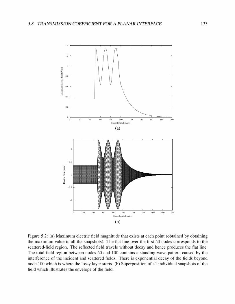
5.8. TRANSMISSION COEFFICIENT FOR A PLANAR INTERFACE 133
0
0.2
0.4
0.6
0.8
1
1.2
1.4
0 20 40 60 80 100 120 140 160 180 200
Max
imu
m E
lect
ric
Fie
ld [
V/m
]
Space [spatial index]
(a)
-1
-0.5
0
0.5
1
0 20 40 60 80 100 120 140 160 180 200
Ele
ctri
c F
ield
[V
/m]
Space [spatial index]
(b)
Figure 5.2: (a) Maximum electric field magnitude that exists at each point (obtained by obtainingthe maximum value in all the snapshots). The flat line over the first 50 nodes corresponds to thescattered-field region. The reflected field travels without decay and hence produces the flat line.The total-field region between nodes 50 and 100 contains a standing-wave pattern caused by theinterference of the incident and scattered fields. There is exponential decay of the fields beyondnode 100 which is where the lossy layer starts. (b) Superposition of 41 individual snapshots of thefield which illustrates the envelope of the field.

134 CHAPTER 5. SCALING FDTD SIMULATIONS TO ANY FREQUENCY
incident
field
reflected
field
transmitted
field
Ez
Ez
Ez
Hy
Hy
Hy
i
i
r
t
r
t
x = 0
m m
Figure 5.3: Planar interface between two media. The interface is at x = 0 and a wave is incidenton the interface from the left. When the impedances of the two media are not matched, a reflectedwave must exist in order to satisfy the boundary conditions.
an imaginary part β, and E+0 is a complex constant that gives the amplitude of the wave (it is
independent of position; the superscript “+” is merely used to emphasize that we are discussing awave propagating in the +x direction). Note that if more than a single frequency is present, E+
0
does not need to be the same for each frequency.More generally, E+
0 will be a function of frequency (we could write this expressly as E+0 (ω) but
the caret implicitly indicates dependence on frequency). To construct a temporal that consists of amultiple frequencies, or even a continuous spectrum of frequencies, one must sum the contributionsfrom each frequency such as is done with a Fourier integral.
In FDTD simulations the time-domain form of the signal is obtained directly. However, oneoften is interested in the behavior of the fields as a function of frequency. As has been discussedin Sec. 5.3, one merely has to take the Fourier transform of a signal to obtain its spectral content.This transform, by itself, is typically of little use. One has to normalize the signal in some way.Knowing what came out of a system is rather meaningless unless one knows what went into thesystem. Here we will work through a couple of simple examples to illustrate how a broad range ofspectral information can be obtained from FDTD simulations.
5.8.1 Transmission through a Planar Interface (Continuous World)Consider the planar interface at x = 0 between two media as depicted in Fig. 5.3. We restrictconsideration to electric polarization in the z direction and assume the incident field originates inthe first medium. In the frequency domain, the incident, reflected, and transmitted fields are givenby
Eiz(x) = E+
a1e−γ1x incident, (5.78)
Erz(x) = E−a1e
+γ1x = ΓE+a1e
+γ1x reflected, (5.79)Etz(x) = E+
a2e−γ2x = T E+
a1e−γ2x transmitted, (5.80)

5.8. TRANSMISSION COEFFICIENT FOR A PLANAR INTERFACE 135
where Γ is the reflection coefficient, T is the transmission coefficient, and γn is the propagationconstant given by jω
√µn(1− jσmn /ωµn)εn(1− jσn/ωεn) where the n indicates the medium and
σm is the magnetic conductivity. The amplitude of the incident field E+a1 is, in general, complex
and a function of frequency. By definition Γ and T are
Γ =Erz(x)
Eiz(x)
∣∣∣∣∣x=0
=E−a1
E+a1
, (5.81)
T =Etz(x)
Eiz(x)
∣∣∣∣∣x=0
=E+a2
E+a1
. (5.82)
The fact that these are defined at x = 0 is important.The magnetic field is related to the electric field by
H iy(x) = − 1
η1
Eiz(x), (5.83)
Hry(x) =
1
η1
Erz(x), (5.84)
H ty(x) = − 1
η2
Etz(x), (5.85)
where the characteristic impedance ηn is given by√µn(1− jσmn /ωµn)/εn(1− jσn/ωεn). Since
the magnetic and electric fields are purely tangential to the planar interface, the sum of the incidentand reflected field at x = 0 must equal the transmitted field at the same point. Matching theboundary condition on the electric field yields
1 + Γ = T , (5.86)
while matching the boundary conditions on the magnetic field produces
1
η1
(1− Γ) =1
η2
T . (5.87)
Solving these for T yields
T =2η2
η1 + η2
. (5.88)
Using this in (5.86) the reflection coefficient is found to be
Γ =η2 − η1
η2 + η1
. (5.89)
5.8.2 Measuring the Transmission Coefficient Using FDTDNow consider two FDTD simulations. The first simulation will be used to record the incidentfield. In this simulation the computational domain is homogeneous and the material propertiescorrespond to that of the first medium. The field is recorded at some observation point x1. Sincenothing is present to interfere with the incident field, the recorded field will be simply the incident

136 CHAPTER 5. SCALING FDTD SIMULATIONS TO ANY FREQUENCY
field at this location, i.e, Eiz(x1, t). In the second simulation, the second medium is present. We
record the fields at the same observation point but we ensure the point was chosen such that it islocated in the second medium (i.e., the interface is to the left of the observation point). Performingan FDTD simulation in this case yields the transmitted field Et
z(x1, t). The goal now is to obtainthe transmission coefficient using the temporal recordings of the field obtained from these twosimulations.
Note that in this section we will not distinguish between the way in which field propagate inthe continuous world and the way in which they propagate in the FDTD grid. In Chap. 7 we willdiscuss in some detail how these differ.
One cannot use Etz(x1, t)/E
iz(x1, t) to obtain the transmission coefficient. The transmission
coefficient is inherently a frequency-domain concept and currently we have time-domain signals.The division of these temporal signals is essentially meaningless (e.g., the result is undefined whenthe incident signal is zero).
The incident and transmitted fields must be converted to the frequency domain using a Fouriertransform. Thus one obtains
Eiz(x1) = F
(Eiz(x1, t)
), (5.90)
Etz(x1) = F
(Etz(x1, t)
), (5.91)
where F indicates the Fourier transform. The division of these two functions is meaningful—atleast at all frequencies where Ei
z(x1) is non-zero. (At frequencies where Eiz(x1) is zero, there is
no incident spectral energy and hence one cannot obtain the transmitted field at those particularfrequencies. In practice it is relatively easy to introduce energy into an FDTD grid that spans abroad range of frequencies.)
Since the observation point was not specified to be on the boundary, the ratio of these fieldfields is
Etz(x1)
Eiz(x1)
=E+a2e−γ2x1
E+a1e−γ1x1
=E+a2
E+a1
e(γ1−γ2)x1 = T e(γ1−γ2)x1 . (5.92)
Solving this for T yields
T (ω) = e(γ2−γ1)x1Etz(x1)
Eiz(x1)
. (5.93)
To demonstrate how the transmission coefficient can be reconstructed from FDTD simulations,let us consider an example where the first medium is free space and the second one has a relativepermittivity εr of 9. In this case γ1 = jω
√µ0ε0 = jβ0 and γ2 = jω
√µ09ε0 = j3β0. Therefore
(5.93) becomes
T (ω) = ej(3β0−β0)x1Etz(x1)
Eiz(x1)
= ej2β0x1Etz(x1)
Eiz(x1)
. (5.94)
The terms in the exponent can be written
2β0x1 = 22π
λx1 =
4π
Nλ∆x
N1∆x =4π
Nλ
N1 (5.95)
where N1 is the number of spatial steps between the interface and the observation point at x1 and,as was discussed in Chap. 5, Nλ is the number of spatial steps per a free-space wavelength of λ.

5.8. TRANSMISSION COEFFICIENT FOR A PLANAR INTERFACE 137
The continuous-world transmission coefficient can be calculated quite easily from (5.88) andthis provides a reference solution. Ideally the FDTD simulation would yield this same value forall frequencies. For this particular example the characteristic impedance of the first medium isη1 = η0 while for the second medium it is η2 = η0/3. Thus the transmission coefficient is
Texact =2η0/3
η0 + η0/3= 1/2. (5.96)
Note that this is a real number and independent of frequency (so the tilde on T is somewhat mis-leading).
For the FDTD simulations, let us record the field 80 spatial steps away from the interface, i.e.,N1 = 80, and run the simulation for 8192 time steps, i.e., NT = 8192. The simulation is run at theCourant limit Sc = 1. The source is a Ricker wavelet discretized so that the peak spectral contentexists at 50 points per wavelength (NP = 50). From Sec. 5.3, recall the relationship between thepoints per wavelength Nλ and frequency index Nfreq which is repeated below:
Nfreq =NT
Nλ
Sc. (5.97)
With a Courant number of unity and 8192 time steps, the points per wavelength for any givenfrequency (or spectral index) is given by
Nλ =8192
Nfreq
. (5.98)
Combining this with (5.93) and (5.95) yields
TFDTD = ej(
4πN1Nfreq8192
)Etz(x1)
Eiz(x1)
. (5.99)
Ideally (5.96) and (5.99) will agree at all frequencies. To see if that is the case, Fig. 5.4 showsthree plots related to the incident and transmitted fields. Figure 5.4(a) shows the first 500 timesteps of the temporal signals recorded at the observation point both with and without the interfacepresent (i.e., the transmitted and incident fields, respectively). Figure 5.4(b) shows the magnitudeof the Fourier transforms of the incident and transmitted fields for the first 500 frequencies. Sincea Ricker wavelet was used, the spectra are essentially in accordance with the discussion of Sec.5.2.3. There is no spectral energy at dc and the spectral content exponentially approaches zero athigh frequencies.
Figure 5.4(c) plots the magnitude of the ratio of the transmitted and incident field as a functionof frequency. Ideally this would be 1/2 for all frequencies. Note the rather small vertical scale ofthe plot. Near dc the normalized transmitted field differs rather significantly from the ideal value,but this is in a region where the results should not be trusted because there is not enough incidentenergy at these frequencies. At the higher frequencies some oscillations are present. The normal-ized field generally remains within two percent of the ideal value over this range of frequencies.
Figure 5.5(a) provides the same information as Fig. 5.4(c) except now the result is plottedversus the discretization Nλ. In this figure dc is off the scale to the right (since in theory dc has aninfinite number of points per wavelength). As the frequency goes up, the wavelength gets shorter

138 CHAPTER 5. SCALING FDTD SIMULATIONS TO ANY FREQUENCY
0 50 100 150 200 250 300 350 400 450 500−0.5
0
0.5
1
1.5
Temporal Index
Ez[ x
1, t]V
/m
(a) Temporal Fields
Incident field Transmitted field
0 50 100 150 200 250 300 350 400 450 5000
5
10
15
20
25
Frequency Index
| E
z[ x
1,ω
]|
(b) Transform vs. Frequency Index
Incident field Transmitted field
0 50 100 150 200 250 300 350 400 450 5000.44
0.46
0.48
0.5
0.52
0.54
Frequency Index
| E
t z[ x
1,ω
]/ E
i z[ x
1,ω
]|
(c) Normalized Transmitted Field vs. Frequency Index
Figure 5.4: (a) Time-domain fields at the observation point both with and the without the interfacepresent. The field without the interface is the incident field and the one with the interface is thetransmitted field. (b) Magnitude of the Fourier transforms of the incident and transmitted fields.The transforms are plotted versus the frequency index Nfreq. It can be seen that the fields do nothave much spectral content near dc nor at high frequencies. (c) Magnitude of the transmitted fieldnormalized by the incident field versus the frequency index. Ideally this would be 1/2 for allfrequencies. Errors are clearly evident when the spectral content of the incident field is small.

5.8. TRANSMISSION COEFFICIENT FOR A PLANAR INTERFACE 139
and hence the number of points per wavelength decreases. Thus high frequencies are to the leftand low frequencies are to the right. The highest frequency in this plot corresponds to an Nfreq of500. In terms of the discretization, this is Nλ = NT/Nfreq = 16.384. This may not seem like aparticularly coarse discretization, but one needs to keep in mind that this is the discretization infrees pace. Within the dielectric, which here has εr = 9, the wavelength is three times smallerand hence within the dielectric the fields are only discretized at approximately five points perwavelength (which is considered a very coarse discretization). From this figure it is clear thatthe FDTD simulations provide results which are close to the ideal over a fairly broad range offrequencies.
Figure 5.5(b) shows the real and imaginary part of the reflection coefficient, i.e., TFDTD definedin (5.99), as a function of the discretization. Ideally the imaginary part would be zero and the realpart would be 1/2. As can be seen, although the magnitude of the transmission coefficient is nearly1/2 over the entire spectrum, the phase differs rather significantly as the discretization decreases(i.e., the frequency increases).
The Matlab code used to generate Fig. 5.4 is shown in Program 5.3 while the code which gen-erated Fig. 5.5 is given in Program 5.4. It is assumed the incident field from the FDTD simulationis recorded to a file named inc-8192 while the transmitted field, i.e., the field when the dielectricis present, is recorded in die-8192. The code in Program 5.3 has to be run prior to that of 5.4 inorder to load and initialize the data.
Let us now consider the same scenario but let the observation point be four steps away fromthe boundary instead of 80, i.e., N1 = 4. Following the previous steps, the incident and transmittedfields are recorded, their transforms are taken, then divided, and finally the phase is adjusted toobtain the transmission coefficient. The result for this observation point is shown in Fig. 5.6. Thereal and imaginary parts stay closer to the ideal values over a larger range of frequencies thanwhen the observation point was 80 cells from the boundary. The fact that the quality of the resultsare frequency sensitive as well as sensitive to the observation point is a consequence of numericdispersion in the FDTD grid, i.e., different frequencies propagate at different speeds. (This is thesubject of Chap. 7.)
Program 5.3 Matlab session used to generate Fig. 5.4.
1 incTime = dlmread(’inc-8192’); % incident field file2 dieTime = dlmread(’die-8192’); % transmitted field file3
4 inc = fft(incTime); % take Fourier transforms5 die = fft(dieTime);6
7 nSteps = length(incTime); % number of time steps8 freqMin = 1; % minimun frequency index of interest9 freqMax = 500; % maximum frequency of interest
10 freqIndex = freqMin:freqMax; % range of frequencies of interest11 % correct for offset of 1 in matlab’s indexing12 freqSlice = freqIndex + 1;13 courantNumber = 1;14 % points per wavelength for freqencies of interest

140 CHAPTER 5. SCALING FDTD SIMULATIONS TO ANY FREQUENCY
0 50 100 150 200 250 3000
0.1
0.2
0.3
0.4
0.5
0.6
0.7
0.8
0.9
1
Points per Wavelength
| E
t z[ x
1,ω
]/ E
i z[ x
1,ω
]|
(a) Normalized Transmitted Field vs. Discretization
0 50 100 150 200 250 300−1
−0.8
−0.6
−0.4
−0.2
0
0.2
0.4
0.6
0.8
1
Points per Wavelength
Tra
nsm
issio
n C
oe
ffic
ien
t, T
(ω)
(a) Real and Imaginary Part of Transmission Coefficient
Real part Imaginary part
Figure 5.5: (a) The magnitude of the normalized transmitted field as a function of the (free space)discretization Nλ. Ideally this would be 1/2 for all discretizations. (b) Real and imaginary part ofthe transmission coefficient transformed back to the interface x = 0 versus discretization. Ideallythe real part would be 1/2 and the imaginary part would be zero for all discretization. For theseplots the observation point was 80 cells from the interface (N1 = 80).
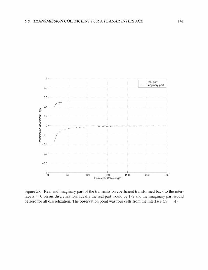
5.8. TRANSMISSION COEFFICIENT FOR A PLANAR INTERFACE 141
0 50 100 150 200 250 300−1
−0.8
−0.6
−0.4
−0.2
0
0.2
0.4
0.6
0.8
1
Points per Wavelength
Tra
nsm
issio
n C
oe
ffic
ien
t, T
(ω)
Real part Imaginary part
Figure 5.6: Real and imaginary part of the transmission coefficient transformed back to the inter-face x = 0 versus discretization. Ideally the real part would be 1/2 and the imaginary part wouldbe zero for all discretization. The observation point was four cells from the interface (N1 = 4).

142 CHAPTER 5. SCALING FDTD SIMULATIONS TO ANY FREQUENCY
15 nLambda = nSteps ./ freqIndex * courantNumber;16 clf17 subplot(3, 1, 1)18 hold on19 plot(incTime(freqSlice), ’-.’);20 plot(dieTime(freqSlice));21 legend(’Incident field’, ’Transmitted field’);22 xlabel(’Temporal Index’);23 ylabel(’\it E_z[\it x_1,\it t] V/m’);24 title(’(a) Temporal Fields’);25
26 subplot(3,1,2)27 hold on28 plot(freqIndex, abs(inc(freqSlice)), ’-.’);29 plot(freqIndex, abs(die(freqSlice)));30 legend(’Incident field’, ’Transmitted field’);31 xlabel(’Frequency Index’);32 ylabel(’|\it E_z[\it x_1,\omega]|’);33 title(’(b) Transform vs. Frequency Index’);34 hold off35
36 subplot(3, 1, 3)37 hold on38 plot(freqIndex, abs(die(freqSlice) ./ inc(freqSlice)));39 xlabel(’Frequency Index’);40 ylabel(’|\it Eˆt_z[\it x_1,\omega]/...41 \it Eˆi_z[\it x_1,\omega]|’);42 title(’(c) Normalized Transmitted Field vs. Frequency Index’);43 hold off
Program 5.4 Matlab session used to generate Fig. 5.5. The commands shown in Program 5.3would have to be run prior to these commands in order to read the data, generate the Fouriertransforms, etc.
1 clf2
3 subplot(2, 1, 1)4 hold on5 plot(nLambda, abs(die(freqSlice) ./ inc(freqSlice)));6 xlabel(’Points per Wavelength’);7 ylabel(’|\it Eˆt_z[\it x_1,\omega]/...8 \it Eˆi_z[\it x_1,\omega]|’);9 title(’(a) Normalized Transmitted Field vs. Discretization’);
10 axis([0 300 0 1])

5.8. TRANSMISSION COEFFICIENT FOR A PLANAR INTERFACE 143
11 hold off12
13 % Array obtained from exp() must be transposed to make arrays14 % conformal. Simply using ’ (a prime) for trasposition will yield15 % the conjugate transpose. Instead, use .’ (dot-prime) to get16 % transposition without conjugation.17 subplot(2, 1, 2)18 hold on19 plot(nLambda, real(exp(j*pi*freqIndex/25.6).’ .* ...20 die(freqSlice) ./ inc(freqSlice)));21 plot(nLambda, imag(exp(j*pi*freqIndex/25.6).’ .* ...22 die(freqSlice) ./ inc(freqSlice)), ’-.’);23 xlabel(’Points per Wavelength’);24 ylabel(’Transmission Coefficient, \it T(\omega)’);25 title(’(b) Real and Imaginary Part of Transmission Coefficient’);26 legend(’Real part’, ’Imaginary part’);27 axis([0 300 -1 1])28 grid on29 hold off
Although we have only considered the transmission coefficient in this example, the reflectioncoefficient could be obtained in a similar fashion. We have intentionally considered a very simpleproblem in order to be able to compare easily the FDTD solution to the exact solution. How-ever one should keep in mind that the FDTD method could be used to analyze the reflection ortransmission coefficient for a much more complicated scenario, e.g., one in which the materialproperties varied continuously, and perhaps quite erratically (with some discontinuities present),over the transition from one half-space to the next. Provided a sufficiently small spatial step-sizewas used, the FDTD method can solve this problem with essentially no more effort than was usedto model the abrupt interface. However, to obtain the exact solution, one may have to work muchharder.

144 CHAPTER 5. SCALING FDTD SIMULATIONS TO ANY FREQUENCY

Chapter 6
Differential-Equation Based AbsorbingBoundary Conditions
6.1 IntroductionA simple absorbing boundary condition (ABC) was used in Chap. 3 to terminate the grid. It re-lied upon the fact that the fields were propagating in one dimension and the speed of propagationwas such that the fields moved one spatial step for every time step, i.e., the Courant number wasunity. The node on the boundary was updated using the value of the adjacent interior node fromthe previous time step. However, when a dielectric was introduced, and the local speed of propa-gation was no longer equal to c, this ABC ceased to work properly. One would also find in higherdimensions that this simple ABC would not work even in free space. This is because the Courantnumber cannot be unity in higher dimensions and this ABC does not account for fields which maybe obliquely incident on the edge of the grid. The goal now is to find a more general technique toterminate the grid.
Although the ABC we will discuss here is not considered state-of-the-art, it provides a rela-tively simple way to terminate the grid that is more than adequate in many circumstances. Addi-tionally, some of the mathematical tools we will develop in this chapter can be used in the analysisof a wide range of FDTD-related topics.
6.2 The Advection EquationThe wave equation that governs the propagation of the electric field in one dimension is
∂2Ez∂x2
− µε∂2Ez∂t2
= 0, (6.1)(∂2
∂x2− µε ∂
2
∂t2
)Ez = 0. (6.2)
The second form represents the equation in terms of an operator operating onEz where the operatoris enclosed in parentheses. This operator can be factored into the product of two operators and is
Lecture notes by John Schneider. fdtd-abc.tex
145

146 CHAPTER 6. DIFFERENTIAL-EQUATION BASED ABC’S
equivalent to (∂
∂x−√µε ∂
∂t
)(∂
∂x+√µε∂
∂t
)Ez = 0. (6.3)
Note that it does not matter which operator in (6.3) is written first. They commute and will alwaysultimately yield (6.1). If either of these operators acting individually on the field yields zero, thewave equation is automatically satisfied. Thus an Ez that satisfies either of the following equationswill also be a solution to the wave equation:
∂Ez∂x−√µε∂Ez
∂t= 0, (6.4)
∂Ez∂x
+√µε∂Ez∂t
= 0. (6.5)
These equations are sometimes called advection equations. Note that a solution to the wave equa-tion will not simultaneously satisfy both these advection equations (except in trivial cases). It maysatisfy one or the other but not both. In fact, fields may be a solution to the wave equation and yetsatisfy neither of the advection equations.∗
A solution to (6.4) is Ez(t+√µεx), i.e., a wave traveling in the negative x direction. The proof
proceeds along the same lines as the proof given in Sec. 2.16. Equate the argument with ξ so that
ξ = t+√µεx. (6.6)
Derivatives of the argument with respect to time or space are given by
∂ξ
∂t= 1 and
∂ξ
∂x=√µε. (6.7)
Thus,
∂Ez∂x
=∂Ez∂ξ
∂ξ
∂x=√µε∂Ez∂ξ
, (6.8)
∂Ez∂t
=∂Ez∂ξ
∂ξ
∂t=∂Ez∂ξ
. (6.9)
Plugging the right-hand sides of (6.8) and (6.9) into (6.4) yields zero and the equation is satisfied.It is worth mentioning that although Ez(t+
√µεx) is a solution to (6.4), it is not a solution to (6.5).
6.3 Terminating the GridLet us now consider how an advection equation can be used to provide an update equation for anode at the end of the computational domain. Let the node Eq+1
z [0] be the node on the boundaryfor which an update equation is sought. Since interior nodes can be updated before the boundarynode, assume that all the adjacent nodes in space-time are known, i.e., Eq+1
z [1], Eqz [0], and Eq
z [1]are known. At the left end of the grid, the fields should only be traveling to the left. Thus the fieldssatisfy the advection equation (6.4). The finite-difference approximation of this equation providesthe necessary update equation, but the way to discretize the equation is not entirely obvious. A

6.3. TERMINATING THE GRID 147
position, x
write difference equation
about this point
Ez [0]q+1 Ez [1]q+1
Ez [0]q Ez [1]q
time, t
avg. in
time
avg. in
space
avg. in
time
avg. in
space
Figure 6.1: Space-time in the neighborhood of the left end of the grid. Only the electric fields areshown. The open circles indicated where an electric field is needed for the advection equation.Since there are none there, averaging is used to approximate the field at those points.
stable ABC will result if the equation is expanded about the space-time point (∆x/2, (q+1/2)∆t).This point is shown in Fig. 6.1.
At first it seems like this in an unacceptable point about which to expand the advection equationsince moving forward or backward in time or space a half step does not correspond to the locationof an electric field point. To fix this, the electric field will be averaged in either time or spaceto obtain an estimate of the value at the desired location in space-time. For example, to obtainan approximation of Eq+1
z [1/2], the average (Eq+1z [0] + Eq+1
z [1])/2, would be used. Similarly, anapproximation of Eq
z [1/2] would be (Eqz [0] + Eq
z [1])/2. Therefore the temporal derivative wouldbe approximated with the following finite difference:
√µε∂Ez∂t
∣∣∣∣∆x/2,(q+1/2)∆t
≈ √µεEq+1z [0]+Eq+1
z [1]2
− Eqz[0]+Eqz[1]2
∆t
(6.10)
Averaging in time is used to obtain the fields at the proper locations for the spatial finite differ-ence. The resulting finite difference is
∂Ez∂x
∣∣∣∣∆x/2,(q+1/2)∆t
≈Eq+1z [1]+Eqz[1]
2− Eq+1
z [0]+Eqz[0]2
∆x
(6.11)
Combining (6.10) and (6.11) yields the finite-difference form of the advection equation
Eq+1z [1]+Eqz[1]
2− Eq+1
z [0]+Eqz[0]2
∆x
−√µεEq+1z [0]+Eq+1
z [1]2
− Eqz[0]+Eqz[1]2
∆t
= 0. (6.12)
∗As an example, consider Ez(x, t) = cos(ωt) sin(βx) where β = ω√µε.

148 CHAPTER 6. DIFFERENTIAL-EQUATION BASED ABC’S
Letting√µε =
√µrεr/c and solving for Eq+1
z [0] yields
Eq+1z [0] = Eq
z [1] +
Sc√µrεr− 1
Sc√µrεr
+ 1
(Eq+1z [1]− Eq
z [0])
(6.13)
where Sc is the Courant number c∆t/∆x. Equation (6.13) provides a first-order absorbing bound-ary condition that updates the field on the boundary using the values of past and interior fields. Thisis known as a first-order ABC because it was constructed from a first-order differential equation.Note that when Sc/
√µrεr is unity, which would be the case of free space and a unit Courant num-
ber, (6.13) reduces to Eq+1z [0] = Eq
z [1] which is the simple grid-termination technique presentedin Sec. 3.9.
At the other end of the grid, i.e., at the right end of the grid, an equation that is nearly identicalto (6.13) pertains. Equation (6.5) would be expanded in the neighborhood of the last node of thegrid. Although (6.4) and (6.5) differ in the sign of one term, when (6.5) is applied it is “looking”in the negative x direction. That effectively cancels the sign change. Hence the update equationfor the last node in the grid, which is identified here as Eq+1
z [M ], would be
Eq+1z [M ] = Eq
z [M − 1] +
Sc√µrεr− 1
Sc√µrεr
+ 1
(Eq+1z [M − 1]− Eq
z [M ]). (6.14)
Recall that for a lossless medium, the coefficient in the electric-field update equation that mul-tiplied the magnetic fields was ∆t/ε∆x and this could be expressed as Scη0/εr. On the other hand,the coefficient in the magnetic-field update equation that multiplied the electric fields was ∆t/µ∆x
and this could be expressed as Sc/η0µr. Therefore, taking the product of these two coefficients andtaking the square root yields (
∆t
ε∆x
∆t
µ∆x
)1/2
=Sc√µrεr
. (6.15)
Note that this is the term that appears in (6.13) and (6.14). Thus by knowing the update coefficientsthat pertain at the ends of the grid, one can calculate the coefficients that appear in the ABC.
6.4 Implementation of a First-Order ABCProgram 3.6 modeled two half spaces: free space and a dielectric. That program was written asa “monolithic” program with a main() function in which all the calculations were performed.For that program we did not have a suitable way to terminate the grid within the dielectric. Let usre-implement that program but use the modular design that was discussed in Chap. 4 and use theABC presented in the previous section.
Recalling the modular design used to model a lossy layer that was discussed in Sec. 4.9, we sawthat the ABC was so simple there was no need to do any initialization of the ABC. Nevertheless,recalling the code shown in Program 4.17, an ABC initialization function was called, but it merelyreturned without doing anything. Now that we wish to implement a first-order ABC, the ABCinitialization function actually needs to perform some calculations: it will calculate any of theconstants associated with the ABC.

6.4. IMPLEMENTATION OF A FIRST-ORDER ABC 149
Naturally, the code associated with the various “blocks” in our modular design will need tochange from what was presented in Sec. 4.9. However, the overall framework remains essentiallythe same! The arrangement of files associated with our model of halfspace that uses a first-orderABC is shown in Fig. 6.2. Note that this figure and Fig. 4.3 are nearly the same. They both havethe same layout. All the functions have the same name, but the implementation of some of thosefunctions have changed. Note that the file names have changed for the files containing the main()function, the gridInit() function, and the abc() and abcInit() function.
The code associated with the TFSF boundary, the snapshots, the source function, and the updateequations are all unchanged from that which was described in Chap. 4. The grid initializationfunction gridInit() constructs a half-space dielectric consistent with Program 3.6. The codeis shown in Program 6.1.
Program 6.1 gridhalfspace.c: Function to initialize the Grid such that there are two half-spaces: free space to the left and a dielectric with εr = 9 to the right.
1 /* Function to initialize the Grid structure. */2
3 #include "fdtd3.h"4
5 #define EPSR 9.06
7 void gridInit(Grid *g) 8 double imp0 = 377.0;9 int mm;
10
11 SizeX = 200; // size of domain12 MaxTime = 450; // duration of simulation13 Cdtds = 1.0; // Courant number14
15 ALLOC_1D(g->ez, SizeX, double);16 ALLOC_1D(g->ceze, SizeX, double);17 ALLOC_1D(g->cezh, SizeX, double);18 ALLOC_1D(g->hy, SizeX - 1, double);19 ALLOC_1D(g->chyh, SizeX - 1, double);20 ALLOC_1D(g->chye, SizeX - 1, double);21
22 /* set electric-field update coefficients */23 for (mm = 0; mm < SizeX; mm++)24 if (mm < 100) 25 Ceze(mm) = 1.0;26 Cezh(mm) = imp0;27 else 28 Ceze(mm) = 1.0;29 Cezh(mm) = imp0 / EPSR;30 31

150 CHAPTER 6. DIFFERENTIAL-EQUATION BASED ABC’S
abcdemo1.c
main()fdtd3.h
ezinc3.h
ezinc3.c
ezIncInit()
ezInc()
update3.c
updateE3()
updateH3()
gridhalfspace.c
gridInit()
tfsf.c
tfsfInit()
tfsfUpdate()
abcfirst.c
abcInit()
abc()
snapshot.c
snapshotInit()
snapshot()
Figure 6.2: Files associated with the modular implementation of a simulation of a dielectric halfspace. Since a first-order ABC is now being used, some of these files differ from those of Fig. 4.3.Nevertheless, the overall structure of the program is unchanged and all the function names are thesame as before.

6.4. IMPLEMENTATION OF A FIRST-ORDER ABC 151
32 /* set magnetic-field update coefficients */33 for (mm = 0; mm < SizeX - 1; mm++) 34 Chyh(mm) = 1.0;35 Chye(mm) = 1.0 / imp0;36 37
38 return;39
The contents of the file abcdemo1.c are shown in Program 6.2. The difference betweenabcdemo1.c and improved3.c, which is given in Program 4.17, is shown in bold. In fact, theonly change in the code is the location of the call of the ABC function abc(). Function abc() isnow called in line 23 which is after the updating of the electric fields. Since the ABC relies on the“future” value of a neighboring interior electric field, this field must be updated before the node onthe grid boundary can be updated. (The ABC function presented in Program 4.17 could, in fact,have been written in such a way that it would be called after the electric-field update. After all,the first-order ABC reduces to the simple ABC when the Courant number is one and the mediumis free space. Nevertheless, the code in Program 4.17 was written to be consistent with the way inwhich the simple ABC was originally presented in Chap. 3.)
Program 6.2 abcdemo1.c: One-dimensional FDTD simulation employing a first-order ABC(although the actual ABC code is contained in the file abcfirst.c which is shown in Program6.3). The difference between this program and Program 4.17 is shown in bold.
1 /* FDTD simulation where main() is primarily used to call other2 * functions that perform the necessary operations. */3
4 #include "fdtd3.h"5
6 int main()7 8 Grid *g;9
10 ALLOC_1D(g, 1, Grid); // allocate memory for Grid11
12 gridInit(g); // initialize the grid13 abcInit(g); // initialize ABC14 tfsfInit(g); // initialize TFSF boundary15 snapshotInit(g); // initialize snapshots16
17 /* do time stepping */18 for (Time = 0; Time < MaxTime; Time++) 19
20 updateH3(g); // update magnetic field21 tfsfUpdate(g); // correct field on TFSF boundary

152 CHAPTER 6. DIFFERENTIAL-EQUATION BASED ABC’S
22 updateE3(g); // update electric field23 abc(g); // apply ABC -- after E-field update24 snapshot(g); // take a snapshot (if appropriate)25
26 /* end of time-stepping */27
28 return 0;29
The code for abcInit() and abc() is contained in the file abcfirst.c which is shownin Program 6.3. The initialization function calculates the coefficients that appeared in (6.13) and(6.14). Recall from (6.15) that these coefficients can be obtained as a function of the electric- andmagnetic-field update-equation coefficients. Since the material at the left and right side of the gridmay be different, there are separate coefficients for the two sides.
Program 6.3 abcfirst.c: Implementation of a first-order absorbing boundary condition.
1 /* Function to implement a first-order ABC. */2
3 #include "fdtd3.h"4 #include <math.h>5
6 static int initDone = 0;7 static double ezOldLeft = 0.0, ezOldRight = 0.0;8 static double abcCoefLeft, abcCoefRight;9
10 /* Initizalization function for first-order ABC. */11 void abcInit(Grid *g) 12 double temp;13
14 initDone = 1;15
16 /* calculate coefficient on left end of grid */17 temp = sqrt(Cezh(0) * Chye(0));18 abcCoefLeft = (temp - 1.0) / (temp + 1.0);19
20 /* calculate coefficient on right end of grid */21 temp = sqrt(Cezh(SizeX - 1) * Chye(SizeX - 2));22 abcCoefRight = (temp - 1.0) / (temp + 1.0);23
24 return;25 26
27 /* First-order ABC. */28 void abc(Grid *g)

6.5. ABC EXPRESSED USING OPERATOR NOTATION 153
29 /* check if abcInit() has been called */30 if (!initDone) 31 fprintf(stderr,32 "abc: abcInit must be called before abc.\n");33 exit(-1);34 35
36 /* ABC for left side of grid */37 Ez(0) = ezOldLeft + abcCoefLeft * (Ez(1) - Ez(0));38 ezOldLeft = Ez(1);39
40 /* ABC for right side of grid */41 Ez(SizeX - 1) = ezOldRight +42 abcCoefRight * (Ez(SizeX - 2) - Ez(SizeX - 1));43 ezOldRight = Ez(SizeX - 2);44
45 return;46
As shown in (6.13) and (6.14), for the first-order ABC both the “past” and the future valueof the interior neighbor nearest to the boundary are needed. However, once we update the fields,past values are overwritten. Thus, the function abc(), which applies the ABC to the two endsof the grid, locally stores the “past” values of the nodes that are adjacent to the ends of the grid.For the left side of the grid the past neighbor is stored as ezOldLeft and on the right it isstored as ezOldRight. These are static global variables that are retained from one invocation ofabc() to the next. Thus, even though the interior fields have been updated, these past values willstill be available. (Once the nodes at the ends of the grid have been updated, ezOldLeft andezOldRight are set to the current value of the neighboring nodes as shown in lines 38 and 43.When abc() is called next, these are indeed the “old” values of these neighbors.)
Figure 6.3 shows the waterfall plot of the snapshots generated by Program 6.2. One can seethat this is the same as Fig. 3.13 prior to the transmitted field encountering the right end of the grid.After that time there is a reflected field evident in Fig. 3.13 but none is visible here. The ABC hasabsorbed the incident field and hence the grid behaves as if it were infinite. In reality this ABCis only approximate and there is some reflected field at the right boundary. We will return to thispoint in Sec. 6.6
6.5 ABC Expressed Using Operator NotationLet us define an identity operator I , a forward spatial shift operator s1
x, and a backward temporalshift operator s−1
t . When they act on a node in the grid their affect is given by
IEq+1z [m] = Eq+1
z [m] , (6.16)s1xE
q+1z [m] = Eq+1
z [m+ 1] , (6.17)s−1t Eq+1
z [m] = Eqz [m] . (6.18)

154 CHAPTER 6. DIFFERENTIAL-EQUATION BASED ABC’S
0 20 40 60 80 100 120 140 160 180 2000
5
10
15
20
25
30
35
40
45
Space [spatial index]
Tim
e [
fra
me
nu
mb
er]
Figure 6.3: Waterfall plot of the snapshots generated by Program 6.2. Comparing this to Fig. 3.13one sees they are the same until the transmitted field encounters the right end of the grid. At thatpoint 3.13 shows there is a reflected field. However, because of the ABC used here, no reflectedfield is visible.

6.5. ABC EXPRESSED USING OPERATOR NOTATION 155
Note that these operators all commute, e.g., s1xs−1t = s−1
t s1x. Furthermore, the identity operator
times another operator is merely that operator, e.g., Is1x = s1
x likewise II = I . Using theseoperators a spatial average of a node can be represented by
Eq+1z [m] + Eq+1
z [m+ 1]
2=
(I + s1
x
2
)Eq+1z [m] , (6.19)
while a temporal average can be written
Eq+1z [m] + Eq
z [m]
2=
(I + s−1
t
2
)Eq+1z [m] . (6.20)
When applying the advection equation, the finite differences, as originally formulated, neededelectric-field nodes where none were present in space-time. Therefore, averaging had to be usedto obtain approximations to the fields at the desired locations. This required averaging in timefollowed by a spatial finite difference or averaging in space followed by a temporal finite difference.Consider the finite difference approximation to the temporal derivative at the point (∆x/2, (q +1/2)∆t). Starting from the node Eq+1
z [0], this requires adding the node one spatial step to the rightand then dividing by two. Then, going back one step in time, these same two nodes are againaveraged and then subtracted from the previous average. The result is divided by the temporal stepto obtain the temporal finite difference. Expressed in operator notation this is
∂Ez∂t
∣∣∣∣∆x/2,(q+1/2)∆t
=
(I − s−1
t
∆t
)(I + s1
x
2
)Eq+1z [0] (6.21)
=1
2∆t
(I − s−1
t + s1x − s−1
t s1x
)Eq+1z [0] (6.22)
=1
2∆t
(Eq+1z [0]− Eq
z [0] + Eq+1z [1]− Eq
z [1]). (6.23)
The second term in parentheses in (6.21) accomplishes the averaging while the first term in paren-theses yields the temporal finite difference. The result, shown in (6.23), is the same as (6.10) (otherthan the factor of
√µε).
A similar approach can be used for the spatial finite difference about the same point except nowthe averaging is done in time
∂Ez∂x
∣∣∣∣∆x/2,(q+1/2)∆t
=
(s1x − I∆x
)(I + s−1
t
2
)Eq+1z [0] (6.24)
=1
2∆x
(−I + s1
x − s−1t + s−1
t s1x
)Eq+1z [0] (6.25)
=1
2∆x
(−Eq+1
z [0] + Eq+1z [1]− Eq
z [0] + Eqz [1]). (6.26)
This is exactly the same as (6.11).From (6.21) and (6.24) we see the finite-difference form of the advection equation can be
expressed as (s1x − I∆x
)(I + s−1
t
2
)−√µε
(I − s−1
t
∆t
)(I + s1
x
2
)Eq+1z [0] = 0. (6.27)

156 CHAPTER 6. DIFFERENTIAL-EQUATION BASED ABC’S
Solving this equation for Eq+1z [0] yields the update equation (6.13). The term in braces is the
finite-difference equivalent of the first advection operator that appeared on the left-hand side of(6.3).
6.6 Second-Order ABCEquation (6.27) provides an update equation which is, in general, approximate. In many circum-stance the field reflected by a first-order ABC is unacceptably large. A more accurate updateequation can be obtained by applying the advection operator twice. Consider(
∂
∂x−√µε ∂
∂t
)(∂
∂x−√µε ∂
∂t
)Ez = 0. (6.28)
Without employing too many mathematical details, assume the field Ez is not a proper solution tothe advection equation. For example, the speed at which it is propagating is not precisely 1/
√µε.
If the field is close to a proper solution, the advection operator operating on the field should yielda number which is close to zero. However, if the advection operator acts on it again, the resultshould be something smaller still—the equation is closer to the truth.
To demonstrate this, consider a wave Ez(t+x/c′) which is traveling in the negative x directionwith a speed c′ 6= c. Following the notation used in Sec. 6.2, the advection operator operating onthis fields yields (
1
c′− 1
c
)∂Ez∂ξ
. (6.29)
If the advection operator again operates on this, the result is(1
c′− 1
c
)2∂2Ez∂ξ2
. (6.30)
If c and c′ are close, (6.30) will be smaller than (6.29) for a broad class of signals. Hence therepeated application of the advection operator may still only be approximately satisfied, but oneanticipates that it will perform better than the first-order operator alone.
The finite-difference form of the second-order advection operator operating on the nodeEq+1z [0]
is [(s1x − I∆x
)(I + s−1
t
2
)−√µε
(I − s−1
t
∆t
)(I + s1
x
2
)(
s1x − I∆x
)(I + s−1
t
2
)−√µε
(I − s−1
t
∆t
)(I + s1
x
2
)]Eq+1z [0] = 0. (6.31)
One expands this equation and solves for Eq+1z [0] to obtain the second-order ABC. The result is
Eq+1z [0] =
−1
1/S ′c + 2 + S ′c
(1/S ′c − 2 + S ′c)
[Eq+1z [2] + Eq−1
z [0]]
+ 2(S ′c − 1/S ′c)[Eqz [0] + Eq
z [2]− Eq+1z [1]− Eq−1
z [1]]
− 4(1/S ′c + S ′c)Eqz [1] − Eq−1
z [2] (6.32)

6.6. SECOND-ORDER ABC 157
where S ′c = ∆t/(√µε∆x) = Sc/
√µrεr. This update equation requires two interior points at time
step q + 1 as well as the boundary node and these same interior points at time steps q and q − 1.Typically these past values would not be available to use in the update equation and must thereforebe stored in some auxiliary manner such as had to be done in Program 6.3 (there just a singlepoint on either end of the grid needed to be stored). Two 3 × 2 arrays (one used at either end ofthe computational domain) could be used to store the values at the three spatial locations and twoprevious time steps required by (6.32). Alternatively, four 1D arrays (two used at either end) ofthree points each could also be used to stored the old values. (It may be noted that Eq
z [0] would notneed to be stored since it would be available when updating the boundary node. However, for thesake of symmetry when writing the loops which store the boundary values, it is simplest to storethis value explicitly.)
When S ′c is unity, as would be the case for propagation in free space with a Courant number ofunity, (6.32) reduces to
Eq+1z [0] = 2Eq
z [1]− Eq−1z [2] . (6.33)
This may appear odd at first but keep in mind that the field is only traveling to the left and it movesone spatial step per time step, thus Eq
z [1] and Eq−1z [2] are equal. Therefore this effectively reduces
to Eq+1z [0] = Eq
z [1] which is again the original grid termination approach used in Sec. 3.9.As was the case for first-order, for the right side of the grid, the second-order termination is
essentially the same as the one on the left side. One merely uses interior nodes to the left of theboundary instead of to the right.
To demonstrate the improvement realized by using a second-order ABC instead of a first-orderone, consider the same computational domain as was used in Program 6.2, i.e., a pulse is incidentfrom free space to a dielectric half-space with a relative permittivity of 9 which begins at node 100.Figure 6.4 shows the electric field in the computational domain at time-step 550 (MaxTime wasincreased from the 450 shown in Program 6.1). Ideally the transmitted pulse would be perfectlyabsorbed and the reflected fields should be zero. However, for both the first- and second-orderABC’s there is a reflected field, but it is significantly smaller in the case of the second-order ABC.

158 CHAPTER 6. DIFFERENTIAL-EQUATION BASED ABC’S
-0.004
-0.003
-0.002
-0.001
0
0.001
0.002
0.003
0 25 50 75 100 125 150 175 200
Ez (
V/m
)
Spatial index
First-Order ABCSecond-Order ABC
Figure 6.4: Plot of the fields at time step 550 when the grid is terminated with either a first- orsecond-order ABC. This snapshot is taken after the transmitted pulse has encountered the rightedge of the grid. Hence this shows the field reflected by the ABC. Ideally the reflected fieldsshould be zero.
6.7 Implementation of a Second-Order ABCIn order to implement a second-order ABC, one merely has to modify the functions abcInit()and abc(). Thus, none of the code depicted in Fig. 6.2 needs to change except for that whichis directly related to the ABC itself. If instead of using the file abcfirst.c, one uses the codeshown in Program 6.4, which we assume is stored in a file called abcsecond.c, then a second-order ABC will be realized.
Program 6.4 abcsecond.c The abcInit() and abc() functions for implementation of asecond-orde ABC.
1 /* Functions to implement a second-order ABC. */2
3 #include "fdtd3.h"4 #include <math.h>5
6 static int initDone = 0;7 static double *ezOldLeft1, *ezOldLeft2,8 *ezOldRight1, *ezOldRight2;9 static double *abcCoefLeft, *abcCoefRight;
10
11 /* Initizalization function for second-order ABC. */

6.7. IMPLEMENTATION OF A SECOND-ORDER ABC 159
12 void abcInit(Grid *g) 13 double temp1, temp2;14
15 initDone = 1;16
17 ALLOC_1D(ezOldLeft1, 3, double);18 ALLOC_1D(ezOldLeft2, 3, double);19 ALLOC_1D(ezOldRight1, 3, double);20 ALLOC_1D(ezOldRight2, 3, double);21
22 ALLOC_1D(abcCoefLeft, 3, double);23 ALLOC_1D(abcCoefRight, 3, double);24
25 /* calculate coefficients on left end of grid */26 temp1 = sqrt(Cezh(0) * Chye(0));27 temp2 = 1.0 / temp1 + 2.0 + temp1;28 abcCoefLeft[0] = -(1.0 / temp1 - 2.0 + temp1) / temp2;29 abcCoefLeft[1] = -2.0 * (temp1 - 1.0 / temp1) / temp2;30 abcCoefLeft[2] = 4.0 * (temp1 + 1.0 / temp1) / temp2;31
32 /* calculate coefficients on right end of grid */33 temp1 = sqrt(Cezh(SizeX - 1) * Chye(SizeX - 2));34 temp2 = 1.0 / temp1 + 2.0 + temp1;35 abcCoefRight[0] = -(1.0 / temp1 - 2.0 + temp1) / temp2;36 abcCoefRight[1] = -2.0 * (temp1 - 1.0 / temp1) / temp2;37 abcCoefRight[2] = 4.0 * (temp1 + 1.0 / temp1) / temp2;38
39 return;40 41
42 /* Second-order ABC. */43 void abc(Grid *g) 44 int mm;45
46 /* check if abcInit() has been called */47 if (!initDone) 48 fprintf(stderr,49 "abc: abcInit must be called before abc.\n");50 exit(-1);51 52
53 /* ABC for left side of grid */54 Ez(0) = abcCoefLeft[0] * (Ez(2) + ezOldLeft2[0])55 + abcCoefLeft[1] * (ezOldLeft1[0] + ezOldLeft1[2] -56 Ez(1) - ezOldLeft2[1])57 + abcCoefLeft[2] * ezOldLeft1[1] - ezOldLeft2[2];58

160 CHAPTER 6. DIFFERENTIAL-EQUATION BASED ABC’S
59 /* ABC for right side of grid */60 Ez(SizeX-1) =61 abcCoefRight[0] * (Ez(SizeX - 3) + ezOldRight2[0])62 + abcCoefRight[1] * (ezOldRight1[0] + ezOldRight1[2] -63 Ez(SizeX - 2) - ezOldRight2[1])64 + abcCoefRight[2] * ezOldRight1[1] - ezOldRight2[2];65
66 /* update stored fields */67 for (mm = 0; mm < 3; mm++) 68 ezOldLeft2[mm] = ezOldLeft1[mm];69 ezOldLeft1[mm] = Ez(mm);70
71 ezOldRight2[mm] = ezOldRight1[mm];72 ezOldRight1[mm] = Ez(SizeX - 1 - mm);73 74
75 return;76
Lines 7–9 declare six static, global pointers, each of which will ultimately serve as an array ofthree points. Four of the arrays will store previous values of the electric field (two arrays dedicatedto the left side and two to the right). The remaining two arrays store the coefficients used in theABC (one array for the left, one for the right). The memory for these arrays is allocated in theabcInit() function in lines 17–23. That is followed by calculation of the coefficients on thetwo side of the grid.
Within the function abc(), which is called once per time-step, the values of the nodes on theedge of the grid are updated by the statements starting on lines 54 and 60. Finally, starting on line67, the stored values are updated. The array exOldLeft1 represents the field one time-step inthe past while exOldLeft2 represents the field two time-steps in the past. Similar naming isemployed on the right.

Chapter 7
Dispersion, Impedance, Reflection, andTransmission
7.1 IntroductionA dispersion relation gives the relationship between frequency and the speed of propagation. Thisrelationship is rather simple in the continuous world and is reviewed in the next section. Unfor-tunately dispersion in the FDTD is not as simple. Nevertheless, it provides a great deal of insightinto the inherent limitations of the FDTD method and hence it is important that one have at least abasic understanding of it.
The tools developed in the analysis of FDTD dispersion can also be used to determine thecharacteristic impedance of the grid. Furthermore, as will be shown, knowing the dispersion rela-tionship one can obtain exact analytic expressions for the reflection and transmission coefficientsin the FDTD grid.
7.2 Dispersion in the Continuous WorldConsider a plane wave propagating in the +x direction in a lossless medium. In time-harmonicform the temporal and spatial dependence of the wave are given by exp(j[ωt − βx]) where ω isthe frequency and β is the phase constant (wave number). The speed of the wave can be found bydetermining how fast a given point on the wave travels. In this context “point” is taken to meana point of constant phase. The phase is dictated by ωt − βx. Setting this equal to a constant anddifferentiating with respect to time gives
d
dt(ωt− βx) =
d
dt(constant), (7.1)
ω − βdxdt
= 0. (7.2)
In this expression x is taken to be the position which provides a particular phase. In that senseit is not an independent variable. The location x which yields the desired phase will change as a
†Lecture notes by John Schneider. fdtd-dispersion.tex
161

162 CHAPTER 7. DISPERSION, IMPEDANCE, REFLECTION, AND TRANSMISSION
function of time. Therefore, dx/dt is the speed of the wave, or, more properly, the phase speed cp.Solving (7.2) for the phase speed yields
cp =dx
dt=ω
β. (7.3)
This is apparently a function of frequency, but for a plane wave the phase constant β is given byω√µε. Thus the phase speed is
cp =ω
ω√µε
=1
√µrµ0εrε0
=c
√µrεr
(7.4)
where c is the speed of light in free space. Note that, in the continuous world for a lossless medium,the phase speed is independent of frequency and the dispersion relationship is
cp =ω
β=
c√µrεr
. (7.5)
Since c is a constant, and we are assuming µr and εr contact for the given material, all frequenciespropagate at the same speed. Unfortunately this is not the case in the discretized FDTD world—different frequencies have different phase speeds.∗
7.3 Harmonic Representation of the FDTD MethodThe spatial shift-operator sx and the temporal shift-operator st were introduced in Sec. 6.5. Gen-eralizing these slightly, let a fractional superscript represent a corresponding fractional step. Forexample,
s1/2x Hq
y [m] = Hqy
[m+
1
2
], (7.6)
s1/2t E
q+ 12
z [m] = Eq+1z [m] , (7.7)
s−1/2t E
q+ 12
z [m] = Eqz [m] . (7.8)
Using these shift operators the finite-difference version of Ampere’s law (ref. (3.17)) can be written
ε
(s
1/2t − s
−1/2t
∆t
)Eq+ 1
2z [m] =
(s
1/2x − s−1/2
x
∆x
)Hq+ 1
2y [m] . (7.9)
Note that both fields have a temporal index of q+ 1/2. The index can be changed to q if the 1/2 isaccounted for by a temporal shift. Thus Ampere’s law can also be written
s1/2t ε
(s
1/2t − s
−1/2t
∆t
)Eqz [m] = s
1/2t
(s
1/2x − s−1/2
x
∆x
)Hqy [m] . (7.10)
∗Later we will consider FDTD models of materials that are dispersive in the continuous world, i.e., materials forwhich ε or µ are functions of frequency. In fact, we have already considered dispersive behavior to some degree sincelossy materials have phase speeds that are a function of frequency.

7.3. HARMONIC REPRESENTATION OF THE FDTD METHOD 163
Let us define the finite-difference operator ∂i as
∂i =
(s
1/2i − s
−1/2i
∆i
)(7.11)
where i is either x or t. Using this notation the Yee version of Ampere’s law can be written
εs1/2t ∂tE
qz [m] = s
1/2t ∂xH
qy [m] . (7.12)
Rather than obtaining an update equation from this, the goal is to determine the phase speedfor a given frequency. To that end, we assume there is a single harmonic wave propagating suchthat
Eqz [m] = E0e
j(ωq∆t−βm∆x), (7.13)
Hqy [m] = H0e
j(ωq∆t−βm∆x), (7.14)
where β is the phase constant which exists in the FDTD grid and E0 and H0 are constant ampli-tudes. A tilde will be used to indicate quantities in the FDTD grid which will typically (but notalways!) differ from the corresponding value in the continuous world. Thus, the phase constant βin the FDTD grid will differ, in general, from the phase constant β in the continuous world. Aswas done in Sec. 5.8 a caret (hat) will be used to indicate a harmonic quantity.
We will assume the frequency ω is the same in both the FDTD grid and the continuous world.Note that one has complete control over the frequency of the excitation—one merely has to ensurethat the phase of the source changes a particular number of radians every time step. However, onedoes not have control over the phase constant, i.e., the spatial frequency. The grid dictates what βwill be for a given temporal frequency.
The plane-wave space-time dependence which appears in (7.13) and (7.14) essentially servesas an eigenfunction for the FDTD governing equations. If the governing equations operate on afunction with this dependence, they will yield another function which has the same space-timedependence, albeit scaled by some value. To illustrate this, consider the temporal shift-operatoracting on the electric field
s±1/2t Eq
z [m] = E0ej[ω(q±1/2)∆t−βm∆x]
= e±jω∆t/2E0ej[ωq∆t−βm∆x]
= e±jω∆t/2Eqz [m] . (7.15)
Similarly, the spatial shift-operator acting on the electric field yields
s±1/2x Eq
z [m] = E0ej[ωq∆t−β(m±1/2)∆x]
= e∓jβ∆x/2E0ej[ωq∆t−βm∆x]
= e∓jβ∆x/2Eqz [m] . (7.16)
Thus, for a plane wave, one can equate the shift operators with multiplication by an appropriateterm:
s±1/2t ⇔ e±jω∆t/2, (7.17)
s±1/2x ⇔ e∓jβ∆x/2. (7.18)

164 CHAPTER 7. DISPERSION, IMPEDANCE, REFLECTION, AND TRANSMISSION
Carrying this a step further, for plane-wave propagation the finite-difference operators ∂t and ∂xare equivalent to
∂t =e+jω∆t/2 − e−jω∆t/2
∆t
= j2
∆t
sin
(ω∆t
2
), (7.19)
∂x =e−jβ∆x/2 − e+jβ∆x/2
∆x
= −j 2
∆x
sin
(β∆x
2
). (7.20)
We define Ω and Kx as
Ω =2
∆t
sin
(ω∆t
2
), (7.21)
Kx =2
∆x
sin
(β∆x
2
). (7.22)
Note that as the discretization goes to zero, Ω approaches ω and Kx approaches β (and, in fact,β would approach β, the phase constant in the continuous world). Using this notation, taking afinite-difference with respect to time is equivalent to multiplication by jΩ while a finite differencewith respect to space is equivalent to multiplication by −jKx, i.e.,
∂t ⇔ jΩ (7.23)∂x ⇔ −jKx. (7.24)
Using (7.17), (7.23), and (7.24) in Ampere’s law (7.12) yields
jεΩejω∆t/2Eqz [m] = −jKxe
jω∆t/2Hqy [m] . (7.25)
The temporal shift exp(jω∆t/2) is common to both side and hence can be canceled. Using theassumed form of the electric and magnetic fields from (7.13) and (7.14) in (7.25) yields
εΩE0ej(ωq∆t−βm∆x) = −KxH0e
j(ωq∆t−βm∆x). (7.26)
Canceling the exponential space-time dependence which is common to both sides produces
εΩE0 = −KxH0. (7.27)
Solving for the ratio of the electric and magnetic field amplitudes yields
E0
H0
= −Kx
εΩ= − ∆t
ε∆x
sin(β∆x
2
)sin(ω∆t
2
) . (7.28)
It appears that (7.28) is the “numeric impedance” since it is the ratio of the electric field to themagnetic field. In fact it is the numeric impedance, but it is only part of the story. As will be shown,the impedance in the FDTD method is exact. This fact is far from obvious if one only considers(7.28). It is also worth considering the corresponding continuous-world quantity β/(εω):
β
εω=ω/cpεω
=1
εcp=
√µε
ε=
õ
ε= η (7.29)
Thus the fact that the grid numeric impedance is given by Kx/(εΩ) is consistent with continuous-world behavior. (The negative sign in (7.28) merely accounts for the orientation of the fields.)

7.4. DISPERSION IN THE FDTD GRID 165
7.4 Dispersion in the FDTD Grid
Another equation relating E0 and H0 can be obtained from Faraday’s law. Expressed in terms ofshift operators, the finite-difference form of Faraday’s law (ref. (3.14)) is
µs1/2x ∂tH
qy [m] = s1/2
x ∂xEqz [m] . (7.30)
As before, assuming plane-wave propagation, the shift operators can be replaced with multiplica-tive equivalents. The resulting equation is
jµΩe−jω∆x/2Hqy [m] = −jKxe
−jω∆x/2Eqz [m] . (7.31)
Canceling terms common to both sides and rearranging yields
E0
H0
= −µΩ
Kx
= −µ∆x
∆t
sin(ω∆t
2
)sin(β∆x
2
) . (7.32)
Equating (7.28) and (7.32) and cross-multiplying gives
µεΩ2 = K2x. (7.33)
This is the FDTD dispersion relation. Alternatively, expanding terms and rearranging slightlyyields
sin2
(ω∆t
2
)=
∆2t
εµ∆2x
sin2
(β∆x
2
). (7.34)
Taking the square root of both sides of either form of the dispersion relation yields√µεΩ = Kx, (7.35)
or
sin
(ω∆t
2
)=
∆t√εµ∆x
sin
(β∆x
2
). (7.36)
These equations dictate the relationship between ω and β. Contrast this to the dispersion relation(7.5) which pertains to the continuous world. The two appear quite dissimilar! However, the twoequations do agree in the limit as the discretization gets small.
The first term in the Taylor series expansion of sin(ξ) is ξ. Thus ξ provides a good approxi-mation of sin(ξ) when ξ is small. Assume that the spatial and temporal steps are small enough sothat the arguments of the sine functions in (7.36) are small. Retaining the first-order term in theTaylor-series expansion of the sine functions in (7.36) yields
ω∆t
2=
∆t√εµ∆x
β∆x
2. (7.37)
From this β is seen to beβ = ω
√µε, (7.38)

166 CHAPTER 7. DISPERSION, IMPEDANCE, REFLECTION, AND TRANSMISSION
which is exactly the same as in the continuous world. However, this is only true when the dis-cretization goes to zero. For finite discretization, the phase speed in the FDTD grid and in thecontinuous world differ.
In the continuous world the phase speed is cp = ω/β. In the FDTD world the same relationholds, i.e., cp = ω/β where the tilde indicates this is the phase speed in the discretized world. Inone dimension, a closed form solution for β is possible (a similar dispersion relation holds in twoand three dimensions, but there a closed-form solution is not possible). Bringing the coefficient tothe other side of (7.36) and taking the arc sine yields
β∆x
2= sin−1
[∆x√µε
∆t
sin
(ω∆t
2
)]. (7.39)
As was shown in Sec. 5.2.2 (ref. (5.7) and (5.8)), the factor ω∆t/2 is equivalent to πSc/Nλ whereSc = c∆t/∆x. Thus (7.39) can be written
β∆x
2= sin−1
[√µrεr
Scsin
(πScNλ
)]. (7.40)
Consider the ratio of the phase speed in the grid to the true phase speed
cpcp
=ω/β
ω/β=β
β=
β∆x
2
β∆x
2
. (7.41)
The phase constant in the continuous world can be written
β = ω√µε = 2π
c
λ
√µ0ε0µrεr =
2π
λ
√µrεr =
2π
Nλ∆x
√µrεr (7.42)
where Nλ is the number of points per free-space wavelength. Using this in the numerator of thelast term on the right-hand side of (7.41) and using (7.40) in the denominator, this ratio becomes
cpcp
=π√µrεr
Nλ sin−1[√
µrεrSc
sin(πScNλ
)] . (7.43)
This equation is a function of the material parameters (εr and µr), the Courant number (Sc), andthe number of points per wavelength (Nλ).
For propagation in free space, i.e., εr = µr = 1, when there are 20 points per wavelength andthe Courant number Sc is 1/2, the ratio of the numeric to the exact phase speed is approximately0.9969 representing an error of 0.31 percent. Thus, for every wavelength of travel, the FDTD wavewill accumulate about 1.12 degrees of phase error (0.0031× 360). If the discretization is loweredto 10 points per wavelength, the ratio drops to 0.9873, or about a 1.27 percent error. Note that asthe discretization was halved, the error increased by roughly a factor of four. This is as should beexpected for a second-order method.
Consider the case of propagation in free space and a Courant number of 1. In that case the ratiocollapses to
cpcp
=π
Nλ sin−1[sin(
πNλ
)] = 1. (7.44)

7.4. DISPERSION IN THE FDTD GRID 167
0.65
0.7
0.75
0.8
0.85
0.9
0.95
1
1.05
2 4 6 8 10 12 14 16 18 20
ph
ase
sp
ee
d r
atio
(F
DT
D/e
xa
ct)
Points per wavelength
Ideal
Courant number 0.75Courant number 0.50Courant number 0.25
Figure 7.1: Ratio of the FDTD and exact phase speeds (cp/cp) versus the discretization. Propa-gation in free space is assumed. Ideally the ratio would be unity for all discretizations. Courantnumbers of 1/4, 1/2, and 3/4 are considered.
Thus the phase speed in the FDTD grid is exactly what it is in the continuous world! This is truefor all discretization.
Figure 7.1 shows a plot of the ratio of the FDTD and exact phase speeds as a function ofdiscretization. Three different Courant numbers are used. Ideally the ratio would be unity for alldiscretizations. As can be seen, the greater the Courant number, the closer the curve is to ideal.A large Courant number is thus desirable for two reasons. First, the larger the Courant number,the greater the temporal step and hence the more quickly a simulation advances (i.e., each updaterepresents a greater advance in time). Second, the larger the Courant number, the smaller thedispersion error. In one dimension a Courant number of unity is the greatest possible and, sincethere is no dispersion error with this Courant number, the corresponding time step is known as themagic time-step. Unfortunately a magic time-step does not exist in higher dimensions.
Figure 7.2 shows snapshots of Ricker wavelets propagating to the right that have been dis-cretized at either 20 or 10 points per wavelength at the most energetic frequency (i.e., the param-eter NP discussed in Sec. 5.2.3 is either 20 or 10). The wavelets are propagating in grids thathave a Courant number of either 1 or 0.5. In Figs. 7.2(a) and (b) the discretizations are 20 and 10,respectively, and the Courant number is unity. Since this corresponds to the magic time-step, thewavelets propagate without distortion. The discretizations in Figs. 7.2(c) and (d) are also 20 and10, respectively, but now the Courant number is 0.5. The snapshots in (a) and (b) were taken after100 time-steps while the snapshots in (c) and (d) were taken after 200 time-steps (since the timestep is half as large in (c) and (d) as it is in (a) and (b), this ensures the snapshots are depictingthe field at the same time). In Fig. 7.2(c) the distortion of the Ricker wavelet is visible in that the

168 CHAPTER 7. DISPERSION, IMPEDANCE, REFLECTION, AND TRANSMISSION
-0.6
-0.4
-0.2
0
0.2
0.4
0.6
0.8
1
0 20 40 60 80 100 120 140 160 180
Ele
ctri
c F
ield
[V
/m]
spatial index
-0.6
-0.4
-0.2
0
0.2
0.4
0.6
0.8
1
0 20 40 60 80 100 120 140 160 180
Ele
ctri
c F
ield
[V
/m]
spatial index
(a) NP = 20, Sc = 1 (b) NP = 10, Sc = 1
-0.6
-0.4
-0.2
0
0.2
0.4
0.6
0.8
1
0 20 40 60 80 100 120 140 160 180
Ele
ctri
c F
ield
[V
/m]
spatial index
-0.6
-0.4
-0.2
0
0.2
0.4
0.6
0.8
1
0 20 40 60 80 100 120 140 160 180
Ele
ctri
c F
ield
[V
/m]
spatial index
(c) NP = 20, Sc = 0.5 (d) NP = 10, Sc = 0.5
Figure 7.2: Snapshots of Ricker wavelets with different discretization propagating in grids withdifferent Courant numbers. (a) 20 points per wavelength at the most energetic frequency, i.e.,NP = 20, Sc = 1, (b) NP = 10, Sc = 1, (c) NP = 20, Sc = 0.5, and (d) NP = 10, Sc = 0.5. Thesnapshots were taken after 100 time-steps for (a) and (b), and after 200 time-steps for (c) and (d).
function is no longer symmetric about the peak. In Fig. 7.2(d) the distortion caused by dispersionis rather extreme and the function is no longer recognizable as a Ricker wavelet. The reason thatFig. 7.2(d) is so much more distorted than Fig. 7.2(c) is that the spectral energy lies at a coarserdiscretization. The more coarsely a harmonic is discretized, the more dispersion it will suffer—thehigher frequencies propagate more slowly than the lower frequencies. This causes the ringing thatis evident on the trailing side of the pulse.

7.5. NUMERIC IMPEDANCE 169
Ez
Hy Hy Hy HyHy
EzEzEzEz
ε1 ε1 ε2 ε2
µ µµ µµ
ε2
Hy
Ez
position, x
x=0transmitted fieldincident + reflected field
Figure 7.3: One-dimensional simulation where the permittivity changes abruptly at x = 0. The in-terface between the two media coincides with a magnetic-field node. The permeability is assumedto be constant throughout the computational domain. The figure depicts the nodes and the materialvalues associated with their updates. The field to the left of the interface is the sum of the incidentand reflected fields. The transmitted field exists to the right of the boundary.
7.5 Numeric ImpedanceLet us return to (7.28) which nominally gave the numeric impedance and which is repeated below
E0
H0
= −Kx
εΩ. (7.45)
The dispersion relation (7.35) expressed Kx in terms of Ω. Plugging this into (7.45) yields
E0
H0
= −√µεΩ
εΩ=
õ
ε= η. (7.46)
Thus, despite the inherent approximations in the FDTD method, the impedance in the grid isexactly the same as in the continuous world (this also holds in higher dimensions).
7.6 Analytic FDTD Reflection and Transmission CoefficientsSection 5.8.2 discussed the way in which an FDTD simulation could be used to measure the trans-mission coefficient associated with a planar interface. In this section, instead of using a simulationto measure the transmission coefficient, an expression will be derived that gives the transmissioncoefficient for the FDTD grid.
Consider a one-dimensional FDTD simulation as shown in Fig. 7.3. The permittivity changesabruptly at the magnetic field which is assumed to coincide with the interface at x = 0. Thepermeability is constant throughout the computational domain.
Assume there is an incident unit-amplitude plane wave propagating in the +x direction. Be-cause of the change in permittivity, a reflected field will exist to the left of the boundary whichpropagates in the −x direction. Additionally, there will be a transmitted field which propagates to

170 CHAPTER 7. DISPERSION, IMPEDANCE, REFLECTION, AND TRANSMISSION
the right of the boundary. The incident, reflected, and transmitted electrics fields are given by
Eiz[m, q] = Ei
z[m]ejωq∆t = e−jβ1m∆xejωq∆t , (7.47)
Erz [m, q] = Er
z [m]ejωq∆t = ˆΓejβ1m∆xejωq∆t , (7.48)
Etz[m, q] = Et
z[m]ejωq∆t = ˆTe−jβ2m∆xejωq∆t (7.49)
where ˆΓ and ˆT are the FDTD reflection and transmission coefficients, respectively. Note that allfields will have the common temporal phase factor exp(jωq∆t). Therefore this term will not beexplicitly written (its existence is implicit in the fact that we are doing harmonic analysis).
As shown in the previous section, the characteristic impedance in the FDTD grid is exact.Therefore the magnetic fields can be related to the electric fields in the same manner as they are inthe continuous world, i.e.,
H iy[m] = − 1
η1
e−jβ1m∆x , (7.50)
Hry [m] =
ˆΓ
η1
ejβ1m∆x , (7.51)
H ty[m] = −
ˆT
η2
e−jβ2m∆x . (7.52)
The incident and reflected waves exist to the left of the interface and the transmitted field existsto the right of the interface. The magnetic field at the interface, i.e., the node at x = 0 is, in a sense,common to both the left and the right half-spaces. The field at this node can be described equallywell as the sum of the incident and reflected waves or by the transmitted wave. This node enforcesthe continuity of the magnetic field across the boundary. Hence, just as in the continuous world,the fields are governed by the equation
− 1
η1
+ˆΓ
η1
= −ˆT
η2
. (7.53)
In the continuous world enforcing the continuity of the tangential electric and magnetic fieldsat a boundary yields two equations. These two equations can be used to solve for the reflectionand transmission coefficients as was shown in Sec. 5.8.1. In FDTD, however, there are no electricfield nodes that coincide with the interface (at least not with this geometry). Therefore continuityof the electric fields cannot be enforced directly nor is there a readily available second equationwith which to solve for the reflection and transmission coefficients.
The necessary second equation is obtained by considering the update equation for the magneticfield at the interface. This node depends on the electric field to either side of the interface and henceties the two half-spaces together. Specifically, the harmonic form of Faraday’s law which governsthe magnetic-field node at the interface can be used to write the following
µs1/2x ∂tH
qy [m]
∣∣∣x=0
= s1/2x ∂xEz[m]
∣∣∣x=0
, (7.54)
µjΩHy[m]∣∣∣x=0
=1
∆x
(s1/2x − s−1/2
x
)Eqz [m]
∣∣∣∣x=0
, (7.55)
jΩHy[m]∣∣∣x=0
=1
µ∆x
(ˆTe−jβ2∆x/2 −
[ejβ1∆x/2 + ˆΓe−jβ1∆x/2
]). (7.56)

7.6. ANALYTIC FDTD REFLECTION AND TRANSMISSION COEFFICIENTS 171
In the last form of the equation, we have used the fact that the transmitted field is present whenspace is shifted a half spatial-step in the +x direction relative to the boundary. Conversely the fieldis the sum of the incident and reflected waves when space is shifted a half spatial-step in the −xdirection relative to the boundary.
Equation (7.56) provides the second equation which, when coupled to (7.53), can be used tosolve for the transmission and reflection coefficients. However, what is Hy[m]
∣∣∣x=0
? Since thisnode is on the interface, the expression for either the transmitted field or the sum of the incidentand reflected field can be used. Using the transmitted field (evaluated at m = 0), the equationbecomes
jΩ
(−
ˆT
η2
)=
1
µ∆x
(ˆTe−jβ2∆x/2 −
[ejβ1∆x/2 + ˆΓe−jβ1∆x/2
]). (7.57)
Regrouping terms yields
ejβ1∆x/2 + ˆΓe−jβ1∆x/2 =
(e−jβ2∆x/2 + j
Ωµ∆x
η2
)ˆT. (7.58)
After multiplying through by −η1 exp(−jβ1∆x/2), (7.53) becomes
e−jβ1∆x/2 − ˆΓe−jβ1∆x/2 =η1
η2
e−jβ1∆x/2 ˆT. (7.59)
Adding the left- and right-hand sides of (7.58) and (7.59) yields an expression that does not dependon the reflection coefficient. Multiplying this expression through by η2 yields
η2
(ejβ1∆x/2 + e−jβ1∆x/2
)=(η1e−jβ1∆x + η2e
−jβ2∆x/2 + jΩµ∆x
)ˆT. (7.60)
Let us consider the third term in parentheses on the right-hand side. Recall from (7.35) that Ω =Kx/√µε. Taking the material and propagation constants that pertain in the second medium,† we
can write
jΩµ∆x = jKx2√µε2
µ∆x, (7.61)
= j
õ
ε2
2
∆x
sin
(β2∆x
2
)∆x, (7.62)
= jη22
(ejβ2∆x/2 − e−jβ2∆x/2
j2
), (7.63)
= η2
(ejβ2∆x/2 − e−jβ2∆x/2
), (7.64)
where (7.22) was used to go from (7.61) to (7.62). Plugging this final form into (7.60), employingEuler’s formula, and solving for the transmission coefficient yields
ˆT =2η2 cos
(β1∆x
2
)η1e−jβ1∆x/2 + η2ejβ2∆x/2
. (7.65)
†As will be more obvious at the end of this derivation, we could instead select the material properties that pertainin the first medium and still obtain the same final result.

172 CHAPTER 7. DISPERSION, IMPEDANCE, REFLECTION, AND TRANSMISSION
This can be compared to the exact transmission coefficient which is given in (5.88). At first itmay appear that these are quite dissimilar. However, if the discretization is sufficiently small, thecosine and complex exponentials are close to unity (and become one as the discretization goesto zero). Hence the FDTD reflection coefficient reduces to the exact reflection coefficient as thediscretization goes to zero.
The complex exponentials in (7.65) make it appear that the FDTD transmission coefficient iscomplex. This would impart a phase shift to the transmitted field that is not present in the contin-uous world. However, this is not the case—(7.65) can be simplified further. The one-dimensionaldispersion relation (7.36) dictates that
sin
(β∆x
2
)=
√εµ∆x
∆t
sin
(ω∆t
2
). (7.66)
Now consider the denominator of (7.65)
η1e−jβ1∆x/2 + η2e
jβ2∆x/2
= η1
(cos
(β1∆x
2
)− j sin
(β1∆x
2
))+ η2
(cos
(β2∆x
2
)+ j sin
(β2∆x
2
))(7.67)
Using (7.66) to convert the sine terms and employing the definition of impedance, the denominatorcan be written
η1 cos
(β1∆x
2
)+ η2 cos
(β2∆x
2
)
−j√µ
ε1
√ε1µ∆x
∆t
sin
(ω∆t
2
)+ j
õ
ε2
√ε2µ∆x
∆t
sin
(ω∆t
2
). (7.68)
Upon canceling the ε’s, the imaginary parts cancel and hence the denominator is purely real. There-fore another expression for the FDTD transmission coefficient is
ˆT =2η2 cos
(β1∆x
2
)η2 cos
(β2∆x
2
)+ η1 cos
(β1∆x
2
) . (7.69)
Combining this with (7.53) yields the reflection coefficient
ˆΓ =η2 cos
(β2∆x
2
)− η1 cos
(β1∆x
2
)η2 cos
(β2∆x
2
)+ η1 cos
(β1∆x
2
) . (7.70)
Because the permeability is assumed to be constant throughout the computational domain, thereflection and transmission coefficients can be written as
ˆT =2√ε1 cos
(β1∆x
2
)√ε1 cos
(β2∆x
2
)+√ε2 cos
(β1∆x
2
) , (7.71)
ˆΓ =
√ε1 cos
(β2∆x
2
)−√ε2 cos
(β1∆x
2
)√ε1 cos
(β2∆x
2
)+√ε2 cos
(β1∆x
2
) . (7.72)

7.7. REFLECTION FROM A PEC 173
10 15 20 25 30 35 40
Points per wavelength, Nλ
−0.42
−0.4
−0.38
−0.36
−0.34
−0.32
Ref
lect
ion C
oef
fici
ent,
Γ
ExactFDTD
ε1 = 1.0 ε
2 = 4.0
Figure 7.4: Reflection coefficient versus discretization for a wave traveling from free space to adielectric with a relative permittivity of 4.0 (i.e., εr1 = 1.0 and εr2 = 4.0). The discretization Nλ
shown on the horizontal axis is that which pertains to free space. (These values should be halvedto give the discretization pertaining to the dielectric.)
Figure 7.4 shows a plot of the FDTD reflection coefficient versus the points per wavelength (infree space) when a wave is incident from free space to a dielectric with a relative permittivity of4.0. For these materials the exact reflection coefficient, which is independent of the discretizationand is also shown in the plot, is Γ = (1− 2)/(1 + 2) = −1/3. When the discretization is 10 pointsper wavelength the FDTD reflection coefficient is nearly −0.42 which corresponds to an error ofapproximately 26 percent. This error is rather large, but one must keep in mind that in the dielectricthe discretization is only five points per wavelength. This coarse discretization affects the qualityof the results throughout the computational domain, not just in the dielectric. Thus, even thoughone may ultimately be interested in the fields over only a portion of the computational domain,nevertheless, one must assure that a proper level of discretization is maintained throughout thegrid.
7.7 Reflection from a PECA perfect electric conductor is realized by setting to zero electric field nodes. Let us assume thatone wants to continue to define the interface as shown in Fig. 7.3, i.e., the boundary is assumedto coincide with a magnetic-field node. The new scenario is shown in Fig. 7.5. The electric-field

174 CHAPTER 7. DISPERSION, IMPEDANCE, REFLECTION, AND TRANSMISSION
Ez
Hy HyHy
Ez=0Ez
ε1 ε1
µ µµHy
Ez
position, x
x=0incident + reflected field
Figure 7.5: One-dimensional space with a perfect electric conductor realized by setting an electricfield node to zero. No fields propagate beyond the zeroed node. The reference point x = 0 is stillassumed to coincide with a magnetic-field node.
node to the right of the interface is set to zero. We now seek to find the reflection coefficient forthis case. There is no transmitted field so the transmission coefficient ˆT must be zero. That mightlead one to think, given (7.53), that the reflection coefficient must be −1 as it is in the continuousworld for a PEC boundary. However, that is not correct. Implicit in (7.53) is the assumption thatthe magnetic field is continuous across the interface. When a PEC is present, this is no longer thecase. In the continuous world the discontinuity in the magnetic field is accounted for by a surfacecurrent.
When a PEC is present there is only one unknown, the reflection coefficient can be obtainedfrom a single equation since the transmission coefficient is known a priori. This equation is pro-vided, as before, by the update equation of the magnetic-field node at the interface. To this end,(7.56) is used with the transmission coefficient set to zero. Also, instead of using the transmittedform of the magnetic field at the interface as was done to obtain (7.57), the sum of the incident andreflected fields is used to obtain:
jΩ
(− 1
η1
+ˆΓ
η1
)=
1
µ∆x
(0−
[ejβ1∆x/2 + ˆΓe−jβ1∆x/2
]). (7.73)
Solving for the reflection coefficient yields
ˆΓPEC =jΩµ∆x − η1e
jβ1∆x/2
jΩµ∆x + η1e−jβ1∆x/2. (7.74)
As was shown in (7.61)–(7.64), the factor jΩµ∆x can be expressed in terms of the impedance and adifference of complex exponentials. Employing such a conversion allows the reflection coefficientto be written as
ˆΓPEC = −e−jβ1∆x . (7.75)
Note that the magnitude of the reflection coefficient is unity so that the entire incident field, regard-less of the frequency, is reflected from the interface.
It appears that the FDTD reflection coefficient for a PEC is introducing a shift that is not presentin the continuous world. However, this is being a bit unfair to the FDTD method. The locationof the PEC boundary really corresponds to the electric-field node that was set to zero. Thus, oneshould really think of the PEC boundary existing at x = ∆x/2.

7.8. INTERFACE ALIGNED WITH AN ELECTRIC-FIELD NODE 175
Ez
Hy Hy Hy HyHy
EzEzEzEz
ε1 ε1 ε2 ε2
µ µµ µµ
εa
Hy
Ez
position, x
x=0transmitted fieldincident + reflected field
Figure 7.6: One-dimensional space with a discontinuity in permittivity. The interface in the con-tinuous world corresponds to an electric-field node in the FDTD grid. The permittivity to the leftof the interface is ε1 and is ε2 to the right. These values are dictated by those in the continuousworld. The permittivity of the node at the interface is εa.
In the continuous world, let us consider a scenario where the origin is located a distance ∆x/2in front of a PEC boundary. In that case the incident and reflected fields must sum to zero atx = ∆x/2, i.e.,
E inc(x) + Eref(x)∣∣x=∆x/2
= 0, (7.76)
e−jβ1∆x/2 + Γejβ1∆x/2 = 0. (7.77)
Thus, in the continuous world the reflection coefficient is
Γ = −e−jβ1∆x . (7.78)
When first comparing (7.75) and (7.78) it may appear that in this case the FDTD reflection coeffi-cient is exact. However the two differ owing to the fact that phase constants β1 and β1 are differentin the two domains.
7.8 Interface Aligned with an Electric-Field NodeThere are situations which necessitate that a discontinuity in permittivity be modeled as coincidingwith an electric field node. The permittivity that should be used to either side of the interface isunambiguous but the permittivity of the node at the interface is open to question since it is neither inone half-space nor the other. This scenario was mentioned in Sec. 3.11 where it was suggested thatthe average permittivity be used for the node at the interface. In this section we wish to providea more rigorous analysis to justify this permittivity. For now, let the permittivity of the node atthe interface be εa as depicted in Fig. 7.6. The goal now is to find the reflection or transmissioncoefficients for this geometry and find the value of εa which yields the best agreement with thecontinuous-world values.
Although the origin x = 0 has shifted from that which was assumed in the previous section,the incident, reflected, and transmitted fields are still assumed to be given by (7.47)–(7.49) and(7.50)–(7.52). The electric-field node at the interface is a member of both half-spaces, i.e., thefield is the same whether considered to be the sum of the incident and reflected field or simply tobe the transmitted field. This yields a boundary condition of
1 + ˆΓ = ˆT. (7.79)

176 CHAPTER 7. DISPERSION, IMPEDANCE, REFLECTION, AND TRANSMISSION
Another equation relating the transmission and reflection coefficients is obtained via the updateequation for the electric-field node at the interface. Ampere’s law evaluated at the interface is
jεaΩˆT =
1
∆x
(−
ˆT
η2
e−jβ2∆x/2 −
[− 1
η1
ejβ1∆x/2 +ˆΓ
η1
e−jβ1∆x/2
]). (7.80)
Using (7.79) ˆT can be replaced with 1 + ˆΓ. Then solving for ˆΓ yields
ˆΓ =η2e
jβ1∆x/2 − η1e−jβ2∆x/2 − jη1η2εaΩ∆x
η2e−jβ1∆x/2 + η1e−jβ2∆x/2 + jη1η2εaΩ∆x
. (7.81)
The term Ω∆x can be written as
Ω∆x =2
∆t
sin
(ω∆t
2
)∆x, (7.82)
= 2c∆x
c∆t
sin
(ω∆t
2
), (7.83)
= 2c1
Scsin
(2πc
Nλ∆x
∆t
2
), (7.84)
= 2c1
Scsin
(π
Nλ
Sc
). (7.85)
The conversion of ω∆t/2 to πSc/Nλ was discussed in connection with (5.74). Using this last formof Ω∆x, the third term in the numerator and denominator of (7.81) can be written
jη1η2εaΩ∆x = j
õ
ε0εr1
õ
ε0εr22cε0εra
1
Scsin
(π
Nλ
Sc
), (7.86)
= jεra√εr1εr2
µ
ε02cε0
1
Scsin
(π
Nλ
Sc
), (7.87)
= jεra√εr1εr2
2µc1
Scsin
(π
Nλ
Sc
), (7.88)
where εra is the relative permittivity of the node at the interface.Assume that the permeability throughout the computational domain is the permeability of free
space so that µc in (7.88) can be written µ0c = µ0/√µ0ε0 =
√µ0/ε0 = η0. The reflection
coefficient (7.81) can now be written as
ˆΓ =
1√εr2η0e
jβ1∆x/2 − 1√εr1η0e−jβ2∆x/2 − j εra√
εr1εr2η0
2Sc
sin(
πNλSc
)1√εr2η0e−jβ1∆x/2 + 1√
εr1η0e−jβ2∆x/2 + j εra√
εr1εr2η0
2Sc
sin(
πNλSc
) . (7.89)
Multiplying numerator and denominator by√εr1εr2/η0 yields
ˆΓ =
√εr1e
jβ1∆x/2 −√εr2e−jβ2∆x/2 − jεra 2Sc
sin(
πNλSc
)√εr1e−jβ1∆x/2 +
√εr2e−jβ2∆x/2 + jεra
2Sc
sin(
πNλSc
) . (7.90)

7.8. INTERFACE ALIGNED WITH AN ELECTRIC-FIELD NODE 177
As is often the case, the expression for a quantity in the FDTD grid bears little resemblance tothat in the continuous world. However, as the discretization goes to zero (i.e., Nλ goes to infinity),(7.90) does indeed reduce to the reflection coefficient in the continuous world.
The first two terms in the numerator and denominator of (7.90) depend on the material constantsto either side of the interface while the third term depends on the permittivity at the interface, theCourant number, and the number of points per wavelength (in continuous-world free space). Wenow seek the value of εa (or the corresponding relative permittivity εra) which minimizes thedifference between the reflection coefficient in the continuous world and the one in the FDTDworld. It is important to note that in general the FDTD reflection coefficient in this case is trulycomplex—there will be a phase shift imparted that does not exist in the continuous world.
Before going further with the analysis, let us consider an example with specific parameters andgraphically solve for the optimum value of εa. Let εr1 = 1, εr2 = 4, and the discretization be10 points per wavelength. In this case the reflection coefficient in the continuous world is −1/3(independent of frequency). Figure 7.7 shows the FDTD reflection coefficient in the complex planefor various values of εra. The continuous-world result, i.e., the exact result, is a single point on thenegative real axis. As εra varies a curve is obtained in the complex plane which is closest to theexact value when εra is 2.5 which is the arithmetic average of 1 and 4. Thus the optimum value forthe interface permittivity is the average of the permittivities to either side. However, these resultsare only for a specific discretization and for one set of permittivities. Is the average value theoptimum one for all permittivities and discretizations?
To answer this question, let us return to (7.81) and separate the numerator and denominatorinto real and imaginary parts. The result is
ˆΓ =η2 cos(κ1)− η1 cos(κ2) + j [η2 sin(κ1) + η1 sin(κ2)− η1η2εaΩ∆x]
η2 cos(κ1) + η1 cos(κ2)− j [η2 sin(κ1) + η1 sin(κ2)− η1η2εaΩ∆x](7.91)
where
κ1 = β1∆x/2, (7.92)κ2 = β2∆x/2. (7.93)
The continuous-world reflection coefficient is purely real and thus any imaginary part is an error.Furthermore, the imaginary part goes to zero as the discretization goes to zero. Let us consider justthis imaginary part of the numerator and denominator. The sin(κ) terms can be related to the Kterms which have been used previously—one merely had to multiply (and divide) by 2/∆x. Thusthe imaginary part can be written
η22
∆x
sin(κ1)∆x
2+η1
2
∆x
sin(κ2)∆x
2−η1η2εaΩ∆x = η1η2
∆x
2
(1
η1
K1 +1
η2
K2 − 2εaΩ
). (7.94)
From the dispersion relation 7.33 we know that K1 =√µε1Ω and K2 =
√µε2Ω. This allows the
imaginary part of the numerator and denominator of the reflection coefficient to be written
η1η2∆x
2Ω (ε1 + ε2 − 2εa) . (7.95)
Setting εa equal to (ε1 + ε2)/2 will yield zero for this imaginary term. Hence the average permit-tivity is the optimum value for all permittivities and discretizations! Using the average permittivity

178 CHAPTER 7. DISPERSION, IMPEDANCE, REFLECTION, AND TRANSMISSION
-0.35 -0.3 -0.25 -0.2 -0.15
Real part of Γ
-0.1
-0.05
0
0.05
0.1
Imag
inar
y p
art
of
Γ
Exact
εra
= 4.0
εra
= 3.5
εra
= 3.0
εra
= 2.5
εra
= 2.0
εra
= 1.5
εra
= 1.0
FDTD
εra
εr1
= 1.0 εr2
= 4.0
Figure 7.7: Curve showing the FDTD reflection coefficient in the complex plane as a functionof εra as εra varies between the relative permittivity to the left of the interface (εra = 1) and therelative permittivity to the right of the interface (εra = 4). The value of εra which minimizes thedifference between the FDTD reflection coefficient and the exact value of −1/3 is the averagepermittivity, i.e., εra = 2.5.

7.8. INTERFACE ALIGNED WITH AN ELECTRIC-FIELD NODE 179
yields reflection and transmission coefficients of
ˆΓ =η2 cos(κ1)− η1 cos(κ2)
η2 cos(κ1) + η1 cos(κ2), (7.96)
ˆT =2η2 cos(κ1)
η2 cos(κ1) + η1 cos(κ2). (7.97)
Note that these equations appear almost identical to those which pertained to the case of an abruptinterface (i.e., when no averaging is done and the resulting reflection and transmission coefficientsare (7.70) and (7.69)). However, these equations differ in the arguments of the cosine terms and,in fact, it can be shown that the abrupt boundary is slightly more accurate than the one which isimplemented with the average permittivity at the interface. Nevertheless, when the situation callsfor the interface to coincide with a tangential electric field, the average permittivity is the optimumone to use.

180 CHAPTER 7. DISPERSION, IMPEDANCE, REFLECTION, AND TRANSMISSION

Chapter 8
Two-Dimensional FDTD Simulations
8.1 IntroductionOne of the truly compelling features of the FDTD method is that the simplicity the method enjoysin one dimension is largely maintained in higher dimensions. The complexity of other numericaltechniques often increases substantially as the number of dimensions increases. With the FDTDmethod, if you understand the algorithm in one dimension, you should have no problem under-standing the basic algorithm in two or three dimensions. Nevertheless, introducing additionaldimensions has to come at the price of some additional complexity.
This chapter provides details concerning the implementation of two-dimensional simulationswith either the magnetic field or the electric field orthogonal to the normal to the plane of propa-gation, i.e., TMz or TEz polarization, respectively. Multidimensional simulations require that wethink in terms of a multidimensional grid and thus we require multidimensional arrays to store thefields. Since we are primarily interested in writing programs in C, we begin with a discussion ofmultidimensional arrays in the C language.
8.2 Multidimensional ArraysWhether an array is one-, two-, or three-dimensional, it ultimately is using a block of contiguousmemory where each element has a single address. The distinction between the different dimensionsis primarily a question of how we want to think about, and access, array elements. For higher-dimensional arrays, we want to specify two, or more, indices to dictate the element of interest.However, regardless of the number of indices, ultimately a single address dictates which memoryis being accessed. The translation of multiple indices to a single address can be left to the compileror that translation is something we can do ourselves.
The code shown in Fragment 8.1 illustrates how one can think and work with what is effec-tively a two-dimensional array even though the memory allocation is essentially the same as wasused with the one-dimensional array considered in Fragment 4.1. In Fragment 8.1 the user isprompted to enter the desired number of rows and columns which are stored in num rows andnum columns, respectively. In line 8 the pointer ez is set to the start of a block of memory
†Lecture notes by John Schneider. fdtd-multidimensional.tex
181

182 CHAPTER 8. TWO-DIMENSIONAL FDTD SIMULATIONS
which can hold num rows × num columns doubles. Thus sufficient space is available to storethe desired number of rows and columns, but this pointer is dereferenced with a single index (oroffset).
Fragment 8.1 Fragment of code demonstrating the construction of a two-dimensional array.
1 #define Ez(I, J) ez[(I) * num_columns + (J)]
...2 double *ez;3 int num_rows, num_columns, m, n;4
5 printf("Enter the number of row and columns: ");6 scanf("%d %d", &num_rows, &num_columns);7
8 ez = calloc(num_rows * num_columns, sizeof(double));9
10 for (m=0; m < num_rows; m++)11 for (n=0; n < num_columns; n++)12 Ez(m, n) = m * n;
In this code the trick to thinking and working in two dimensions, i.e., working with two indicesinstead of one, is the macro which is shown in line 1. This macro tells the preprocessor thatevery time the string Ez appears with two arguments—here the first argument is labeled I and thesecond argument is labeled J—the compiler should translate that to ez[(I) * num columns+ (J)]. Note the uppercase E in Ez distinguishes this from the pointer ez. I and J in themacro are just dummy arguments. They merely specify how the first and second arguments shouldbe used in the translated code. Thus, if Ez(2, 3) appears in the source code, the macro tellsthe preprocessor to translate that to ez[(2) * num columns + (3)]. In this way we havespecified two indices, but the macro translates those indices into an expression which evaluatesto a single number which represents the offset into a one-dimensional array (the array ez). Eventhough Ez is technically a macro, we will refer to it as an array. Note that, as seen in line 12, Ez’sindices are enclosed in parentheses, not brackets.
To illustrate this further, assume the user specified that there are 4 columns (num columns is4) and 3 rows. When the row number increments by one, that corresponds to moving 4 locationsforward in memory. The following shows the arrangement of the two-dimensional array Ez(m,n) where m is used for the row index and n is used for the column index.
n=0 n=1 n=2 n=3m=0 Ez(0, 0) Ez(0, 1) Ez(0, 2) Ez(0, 3)m=1 Ez(1, 0) Ez(1, 1) Ez(1, 2) Ez(1, 3)m=2 Ez(2, 0) Ez(2, 1) Ez(2, 2) Ez(2, 3)
The Ez array really corresponds to the one-dimensional ez array. The macro calculates the indexfor the ez array based on the arguments (i.e., indices) of the Ez array. The following shows thesame table of values, but in terms of the ez array.

8.2. MULTIDIMENSIONAL ARRAYS 183
n=0 n=1 n=2 n=3m=0 ez[0] ez[1] ez[2] ez[3]m=1 ez[4] ez[5] ez[6] ez[7]m=2 ez[8] ez[9] ez[10] ez[11]
Again, in this example, when the row is incremented by one, the array index is incremented by 4(which is the number of columns). This is due to the fact that we are storing the elements by rows.An entire row of values is stored, then the next row, and so on. Each row contains num columnselements.
Instead of storing things by rows, we could have easily employed “column-centric storage”where an entire column is stored contiguously. This would be accomplished by using the macro
#define Ez(I, J) ez[(I) + (J) * num_rows]
This would be used instead of line 1 in Fragment 8.1. If this were used, each time the row isincremented by one the index of ez is incremented by one. If the column is incremented by one,the index of ez would be incremented by num rows. In this case the elements of the ez arraywould correspond to elements of the Ez array as shown below:
n=0 n=1 n=2 n=3m=0 ez[0] ez[3] ez[6] ez[9]m=1 ez[1] ez[4] ez[7] ez[10]m=2 ez[2] ez[5] ez[8] ez[11]
Note that when the row index is incremented by one, the index of ez is also incremented byone. However, when the column is incremented by one, the index of ez is incremented by 3,which is the number of rows. This type of column-centric storage is used in FORTRAN. However,multidimensional arrays in C are generally assumed to be stored in row-order. Thus column-centric storage will not be considered further and we will use row-centric macros similar to theone presented in Fragment 8.1.
When an array is stored by rows, it is most efficient to access the array one row at a time—notone column at a time. Lines 10 through 12 of Fragment 8.1 demonstrate this by using two loops toset the elements of Ez to the product of the row and column indices. The inner loop is over the rowand the outer loop sets the column. This is more efficient than if these loops were interchanged(although there is likely to be no difference for small arrays). This is a consequence of the waymemory is stored both on the disk and in the CPU cache.
Memory is accessed in small chunks known as pages. If the CPU needs access to a certainvariable that is not already in the cache, it will generate a page fault (and servicing a page faulttakes more time than if the variable were already in the cache). When the page gets to the cacheit contains more than just the variable the CPU wanted—it contains other variables which werestored in memory adjacent to the variable of interest (the page may contain many variables). If thesubsequent CPU operations involve a variable that is already in the cache, that operation can bedone very quickly. It is most likely that that variable will be in the cache, and the CPU will nothave to generate a page fault, if that variable is adjacent in memory to the one used in the previousoperation. Thus, assuming row-centric storage, working with arrays row-by-row is the best way toavoid needless page faults.

184 CHAPTER 8. TWO-DIMENSIONAL FDTD SIMULATIONS
It is important to note that we should not feel constrained to visualize our arrays in terms of thestandard way in which arrays are displayed! Typically two-dimensional arrays are displayed in atable with the first element in the upper, left-hand corner of the table. The first index gives the rownumber and the second index gives the column number. FDTD simulations are modeling a physicalspace, not a table of numbers. In two dimensions we will be concerned with spatial dimensions xand y. It is convention to give the x location as the first argument and the y location as the secondargument, i.e., Ez(x, y). It is also often the case that it is convenient to think of the lower left-handcorner of some finite rectangular region of space as the origin. It is perfectly acceptable to usethe array mechanics which have been discussed so far but to imagine them corresponding to anarrangement in space which corresponds to our usual notion of variation in the x and y directions.So, for example, in the case of a 3 by 4 array, one can visualize the nodes as being arranged in thefollowing way:
n=3 Ez(0,3) Ez(1,3) Ez(2,3) n=3 ez[3] ez[7] ez[11]n=2 Ez(0,2) Ez(1,2) Ez(2,2) n=2 ez[2] ez[6] ez[10]n=1 Ez(0,1) Ez(1,1) Ez(2,1) ⇐⇒ n=1 ez[1] ez[5] ez[9]n=0 Ez(0,0) Ez(1,0) Ez(2,0) n=0 ez[0] ez[4] ez[8]
m=0 m=1 m=2 m=0 m=1 m=2
Nothing has changed in terms of the implementation of the macro to realize this two-dimensionalarray—the only difference is the way the elements have been displayed. The depiction here isnatural when thinking in terms of variations in x and y, where the first index corresponds to x andthe second index corresponds to y. The previous depiction was natural to the way most peoplediscuss tables of data. Regardless of how we think of the arrays, it is still true that the second indexis the one that should vary most rapidly in the case of nested loops (i.e., one should strive to haveconsecutive operations access consecutive elements in memory).
As mentioned in Sec. 4.2, it is always best to check that an allocation of memory was success-ful. If calloc() is unable to allocated the requested memory, it will return NULL. After everyallocation we could add code to check that the request was successful. However, as we did inone-dimension, a better approach is again offered with the use of macros. Fragment 8.2 shows amacro that can be used to allocate memory for a two-dimensional array.
Fragment 8.2 Macro for allocating memory for a two-dimensional array.
1 #define ALLOC_2D(PNTR, NUMX, NUMY, TYPE) \2 PNTR = (TYPE *)calloc((NUMX) * (NUMY), sizeof(TYPE)); \3 if (!PNTR) \4 perror("ALLOC_2D"); \5 fprintf(stderr, \6 "Allocation failed for " #PNTR ". Terminating...\n");\7 exit(-1); \8
The macro ALLOC 2D() is similar to ALLOC 1D(), which was presented in Fragment 4.2, exceptit takes four arguments instead of three. The first argument is a pointer, the second is the number

8.3. TWO DIMENSIONS: TMZ POLARIZATION 185
of rows, the third is the number of columns, and the fourth is the data type. As an example of howthis macro could be used, line 8 of Fragment 8.1 could be replaced with
ALLOC_2D(ez, num_rows, num_columns, double);
8.3 Two Dimensions: TMz PolarizationThe one-dimensional problems considered thus far assumed a non-zero z component of the electricfield and variation only in the x direction. This required the existence of a non-zero y componentof the magnetic field. Here the field is assumed to vary in both the x and y directions, but not thez direction. From the outset we will include the possibility of a magnetic conductivity σm. Withthese assumptions Faraday’s law becomes
−σmH− µ∂H
∂t= ∇× E =
∣∣∣∣∣∣ax ay az∂∂x
∂∂y
0
0 0 Ez
∣∣∣∣∣∣ = ax∂Ez∂y− ay
∂Ez∂x
. (8.1)
Since the right-hand side only has non-zero components in the x and y directions, the time-varyingcomponents of the magnetic field can only have non-zero x and y components (we are not con-cerned with static fields nor a rather pathological case where the magnetic current σmH cancelsthe time-varying field ∂H/∂t). The magnetic field is transverse to the z direction and hence this isdesignated the TMz case. Ampere’s law becomes
σE + ε∂E
∂t= ∇×H =
∣∣∣∣∣∣ax ay az∂∂x
∂∂y
0
Hx Hy 0
∣∣∣∣∣∣ = az
(∂Hy
∂x− ∂Hx
∂y
). (8.2)
The scalar equations obtained from (8.1) and (8.2) are
−σmHx − µ∂Hx
∂t=
∂Ez∂y
, (8.3)
σmHy + µ∂Hy
∂t=
∂Ez∂x
, (8.4)
σEz + ε∂Ez∂t
=∂Hy
∂x− ∂Hx
∂y. (8.5)
Note that, ignoring the conduction terms for a moment, the temporal derivative of the magneticfield is related to the spatial derivative of the electric field and vice versa. The only differencefrom the one-dimensional case is the additional field component Hx and the derivatives in the ydirection.
Space-time is now discretized so that (8.3)–(8.5) can be expressed in terms of finite-differences.From these difference equations the future fields can be expressed in terms of past fields. Followingthe notation used in Sec. 3.3, the following notation will be used:
Hx(x, y, t) = Hx(m∆x, n∆y, q∆t) = Hqx[m,n] , (8.6)
Hy(x, y, t) = Hy(m∆x, n∆y, q∆t) = Hqy [m,n] , (8.7)
Ez(x, y, t) = Ez(m∆x, n∆y, q∆t) = Eqz [m,n] . (8.8)

186 CHAPTER 8. TWO-DIMENSIONAL FDTD SIMULATIONS
As before, the index m corresponds to the spatial step in the x direction while the index q corre-sponds to the temporal step. Additionally the index n represents the spatial step in the y direction.The spatial step sizes in the x and y directions are ∆x and ∆y, respectively (these need not beequal).
In order to obtain the necessary update-equations, each of the field components must be stag-gered in space. However, it is not necessary to stagger all the field components in time. The electricfield must be offset from the magnetic field, but the magnetic field components do not need to bestaggered relative to each other—all the magnetic field components can exist at the same time. Asuitable spatial staggering of the electric and magnetic field components is shown in Fig. 8.1.
When we say the dimensions of a TMz grid is M × N , that corresponds to the dimensionsof the Ez array. We will ensure the grid is terminated such that there are electric-field nodes onthe edge of the grid. Thus, the Hx array would by M × (N − 1) while the Hy array would be(M − 1)×N .
In the arrangement of nodes shown in Fig. 8.1 we will assume the electric field nodes fall atinteger spatial steps and the magnetic field nodes are offset a half spatial step in either the x or ydirection. As with one dimension, the electric field is assumed to exist at integer multiples of thetemporal step while both magnetic fields components are offset a half time-step from the electricfields. With this arrangement in mind, the finite difference approximation of (8.3) expanded aboutthe space-time point (m∆x, (n+ 1/2)∆y, q∆t) is
−σmHq+ 1
2x
[m,n+ 1
2
]+H
q− 12
x
[m,n+ 1
2
]2
− µHq+ 1
2x
[m,n+ 1
2
]−Hq− 1
2x
[m,n+ 1
2
]∆t
=
Eqz [m,n+ 1]− Eq
z [m,n]
∆y
. (8.9)
This can be solved for the future valueHq+ 1
2x
[m,n+ 1
2
]in terms of the “past” values. The resulting
update equation is
Hq+ 1
2x
[m,n+
1
2
]=
1− σm∆t
2µ
1 + σm∆t
2µ
Hq− 1
2x
[m,n+
1
2
]− 1
1 + σm∆t
2µ
∆t
µ∆y
(Eqz [m,n+ 1]− Eq
z [m,n]) .
(8.10)As was the case in one dimension, the material parameters µ and σm are those which pertain at thegiven evaluation point.
The update equation for the y component of the magnetic field is obtained by the finite-difference approximation of (8.4) expanded about the space-time point ((m+ 1/2)∆x, n∆y, q∆t).The resulting equation is
Hq+ 1
2y
[m+
1
2, n
]=
1− σm∆t
2µ
1 + σm∆t
2µ
Hq− 1
2y
[m+
1
2, n
]+
1
1 + σm∆t
2µ
∆t
µ∆x
(Eqz [m+ 1, n]− Eq
z [m,n]) .
(8.11)Again, the material parameters µ and σm are those which pertain at the given evaluation point.Note that Hy nodes are offset in space from Hx nodes. Hence the µ and σm appearing in (8.10)and (8.11) are not necessarily the same even when m and n are the same.

8.3. TWO DIMENSIONS: TMZ POLARIZATION 187
sameindices
sameindices
sameindices
sameindices
sameindices
∆x
∆y
Ez(m,n)
y
xz
Hy(m,n)
Hx(m,n)
Ez(m,n)Hy(m+1/2,n)
Hx(m,n+1/2)
y
xz
Figure 8.1: Spatial arrangement of electric- and magnetic-field nodes for TMz polarization. Theelectric-field nodes are shown as circles and the magnetic-field nodes as squares with a line thatindicates the orientation of the field component. The somewhat triangularly shaped dashed linesindicate groupings of nodes that have the same array indices. For example, in the lower left cornerof the grid all the nodes would have indices in a computer program of (m = 0, n = 0). In thiscase the spatial offset of the fields is implicitly understood. This grouping is repeated throughoutthe grid. However, groups at the top of the grid lack an Hx node and groups at the right edge lackan Hy node. The diagram at the bottom left of the figure indicates nodes with their offsets givenexplicitly in the spatial arguments whereas the diagram at the bottom right indicates how the samenodes would be specified in a computer program where the offsets are understood implicitly.

188 CHAPTER 8. TWO-DIMENSIONAL FDTD SIMULATIONS
The electric-field update equation is obtained via the finite-difference approximation of (8.5)expanded about (m∆x, n∆y, (q + 1/2)∆t):
Eq+1z [m,n] =
1− σ∆t
2ε
1 + σ∆t
2ε
Eqz [m,n] +
1
1 + σ∆t
2ε
(∆t
ε∆x
Hq+ 1
2y
[m+
1
2, n
]−Hq+ 1
2y
[m− 1
2, n
]− ∆t
ε∆y
Hq+ 1
2x
[m,n+
1
2
]−Hq+ 1
2x
[m,n− 1
2
]). (8.12)
A uniform grid is one in which the spatial step size is the same in all directions. Assuming auniform grid such that ∆x = ∆y = δ, we define the following quantities
Chxh(m,n+ 1/2) =1− σm∆t
2µ
1 + σm∆t
2µ
∣∣∣∣∣mδ,(n+1/2)δ
, (8.13)
Chxe(m,n+ 1/2) =1
1 + σm∆t
2µ
∆t
µδ
∣∣∣∣∣mδ,(n+1/2)δ
, (8.14)
Chyh(m+ 1/2, n) =1− σm∆t
2µ
1 + σm∆t
2µ
∣∣∣∣∣(m+1/2)δ,nδ
, (8.15)
Chye(m+ 1/2, n) =1
1 + σm∆t
2µ
∆t
µδ
∣∣∣∣∣(m+1/2)δ,nδ
, (8.16)
Ceze(m,n) =1− σ∆t
2ε
1 + σ∆t
2ε
∣∣∣∣∣mδ,nδ
, (8.17)
Cezh(m,n) =1
1 + σ∆t
2ε
∆t
εδ
∣∣∣∣∣mδ,nδ
. (8.18)
These quantities appear in the update equations and employ the following naming convention: thefirst letter identifies the quantity as a constant which does not vary in time (one can also think ofthis C as representing the word coefficient), the next two letters indicate the field being updated,and the last letter indicates the type of field this quantity multiplies. For example, Chxh appears inthe update equation for Hx and it multiples the previous value of the magnetic field. On the otherhand, Chxe , which also appears in the update equation for Hx, multiplies the electric fields.
To translate these update equations into a form that is suitable for use in a computer program,we follow the approach that was used in one dimension: explicit references to the time step aredropped and the spatial offsets are understood. As illustrated in Fig. 8.1, an Hy node is assumedto be a half spatial step further in the x direction than the corresponding Ez node with the sameindices. Similarly, anHx node is assumed to be a half spatial step further in the y direction than thecorresponding Ez node with the same indices. Thus, in C, the update equations could be written
Hx(m, n) = Chxh(m, n) * Hx(m, n) -Chxe(m, n) * (Ez(m, n + 1) - Ez(m, n));
Hy(m, n) = Chyh(m, n) * Hy(m, n) +Chye(m, n) * (Ez(m + 1, n) - Ez(m, n));

8.4. TMZ EXAMPLE 189
Ez(m, n) = Ceze(m, n) * Ez(m, n) +Cezh(m, n) * ((Hy(m, n) - Hy(m - 1, n)) - (Hx(m, n) - Hx(m, n - 1)));
The reason that the “arrays” appearing in these equations start with an uppercase letter and useparentheses (instead of two pairs of brackets that would be used with traditional two-dimensionalarrays in C) is because these terms are actually macros consistent with the usage described inSec. 8.2. In order for these equations to be useful, they have to be contained within loops thatcycle over the spatial indices and these loops must themselves be contained within a time-steppingloop. Additional considerations are initialization of the arrays, the introduction of energy, andtermination of the grid. This issues are covered in the following sections.
8.4 TMz ExampleTo illustrate the simplicity of the FDTD method in two dimensions, let us consider a simulation of aTMz grid which is 101 nodes by 81 nodes and filled with free space. The grid will be terminated onelectric field nodes which will be left at zero (so that the simulation is effectively of a rectangularresonator with PEC walls). A Ricker wavelet with 20 points per wavelength at its most energeticfrequency is hardwired to the electric-field node at the center of the grid.
Before we get to the core of the code, we are now at a point where it is convenient to split themain header file into multiple header files: one defining the Grid structure, one defining variousmacros, one giving the allocation macros, and one providing the function prototypes. Not all the“.c” files need to include each of these header files.
The arrangement of the code is shown in Fig. 8.2. In this figure the header files fdtd-grid1.h,fdtd-alloc1.h, fdtd-macro-tmz.h, and fdtd-proto1.h are shown in a single boxbut they exist as four separate files (as will be shown below).
The contents of fdtd-grid1.h are shown in Program 8.3. The Grid structure, whichbegins on line 6, now has elements for any of the possible electric or magnetic field components aswell as their associated coefficient arrays. Note that just because all the pointers are declared, theydo not have to be used or point to anything useful. The Grid structure shown here could be usedfor a 1D simulation—it provides elements for everything that was needed to do a 1D simulation—but most of the pointers would be unused, i.e., those elements that pertain to anything other than a1D simulation would be ignored.
The way we will distinguish between what different grids are being used for is by setting the“type” field of the grid. Note that line 4 creates a GRIDTYPE enumeration. This commandmerely serves to set the value of oneDGrid to zero, the value of teZGrid to one, and the valueof tmZGrid to two. (The value of threeDGrid would be three, but we are not yet concernedwith three-dimensional grids.) A Grid will have its type set to one of these values. Functionscan then check the type and act accordingly.
Program 8.3 fdtd-grid1.h Contents of the header file that defines the Grid structure. Thisstructure now contains pointers for each of the possible field values. However, not all these pointerswould be used for any particular grid. The pointers that are meaningful would be determined bythe “type” of the grid. The type takes on one of the values of the GRIDTYPE enumeration.
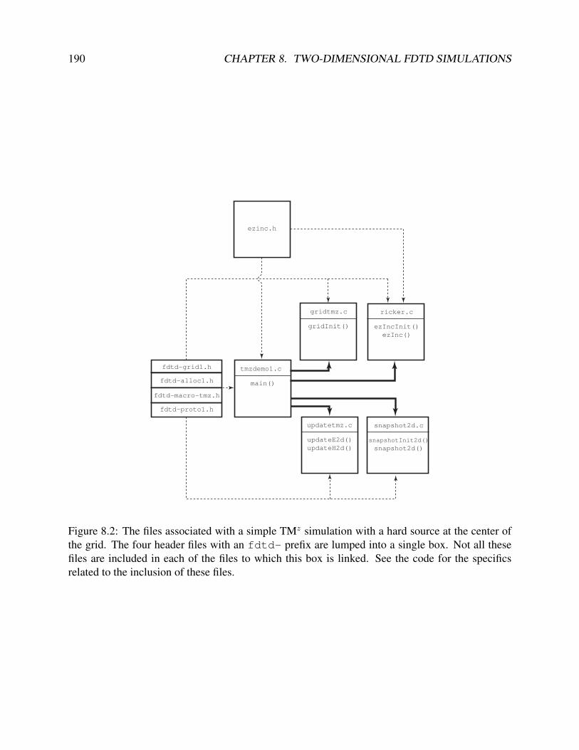
190 CHAPTER 8. TWO-DIMENSIONAL FDTD SIMULATIONS
tmzdemo1.c
main()
fdtd-proto1.h
ezinc.h
ricker.c
ezIncInit()
ezInc()
updatetmz.c
updateE2d()
updateH2d()
gridtmz.c
gridInit()
snapshot2d.c
snapshotInit2d()
snapshot2d()
fdtd-alloc1.h
fdtd-macro-tmz.h
fdtd-grid1.h
Figure 8.2: The files associated with a simple TMz simulation with a hard source at the center ofthe grid. The four header files with an fdtd- prefix are lumped into a single box. Not all thesefiles are included in each of the files to which this box is linked. See the code for the specificsrelated to the inclusion of these files.

8.4. TMZ EXAMPLE 191
1 #ifndef _FDTD_GRID1_H2 #define _FDTD_GRID1_H3
4 enum GRIDTYPE oneDGrid, teZGrid, tmZGrid, threeDGrid;5
6 struct Grid 7 double *hx, *chxh, *chxe;8 double *hy, *chyh, *chye;9 double *hz, *chzh, *chze;
10 double *ex, *cexe, *cexh;11 double *ey, *ceye, *ceyh;12 double *ez, *ceze, *cezh;13 int sizeX, sizeY, sizeZ;14 int time, maxTime;15 int type;16 double cdtds;17 ;18
19 typedef struct Grid Grid;20
21 #endif
The contents of fdtd-alloc1.h are shown in Program 8.4. This header file merely providesthe memory-allocation macros that have been discussed previously.
Program 8.4 fdtd-alloc1.h Contents of the header file that defines the memory allocationmacros suitable for 1D and 2D arrays.
1 #ifndef _FDTD_ALLOC1_H2 #define _FDTD_ALLOC1_H3
4 #include <stdio.h>5 #include <stdlib.h>6
7 /* memory allocation macros */8 #define ALLOC_1D(PNTR, NUM, TYPE) \9 PNTR = (TYPE *)calloc(NUM, sizeof(TYPE)); \
10 if (!PNTR) \11 perror("ALLOC_1D"); \12 fprintf(stderr, \13 "Allocation failed for " #PNTR ". Terminating...\n");\14 exit(-1); \15 16

192 CHAPTER 8. TWO-DIMENSIONAL FDTD SIMULATIONS
17 #define ALLOC_2D(PNTR, NUMX, NUMY, TYPE) \18 PNTR = (TYPE *)calloc((NUMX) * (NUMY), sizeof(TYPE)); \19 if (!PNTR) \20 perror("ALLOC_2D"); \21 fprintf(stderr, \22 "Allocation failed for " #PNTR ". Terminating...\n");\23 exit(-1); \24 25
26 #endif
The contents of fdtd-macro-tmz.h are shown in Program 8.5. This file provides themacros used to access the field arrays and elements of a pointer to a Grid structure. Thus far allthe macros we have used assumed the Grid pointer was called g. The macros provided in lines8–35 no longer make this assumption. Instead, one specifies the name of the pointer as the firstargument. To this point in our code there is no need for this added degree of freedom. We onlyconsidered code that has one pointer to a Grid and we have consistently named it g. However,as we will see when we discuss the TFSF boundary, it is convenient to have the ability to refer todifferent grids.
The macros in lines 39–66 do assume the Grid pointer is named g. These macros are actuallydefined in terms of the first set of macros where the first argument has been set to g. Note thatalthough we are discussing a 2D TMz problem, this file still provides macros that can be used fora 1D array. Again, we will see, when we implement a 2D TFSF boundary, that there are validreasons for doing this. Since any function that is using these macros will also need to know abouta Grid structure, line 4 ensures that the fdtd-grid1.h header file is also included.
Program 8.5 fdtd-macro-tmz.h Header file providing macros suitable for accessing the el-ements and arrays of either a 1D or 2D Grid. There are two distinct sets of macros. The firstset takes an argument that speficies the name of the pointer to the Grid structure. The second setassumes the name of the pointer is g.
1 #ifndef _FDTD_MACRO_TMZ_H2 #define _FDTD_MACRO_TMZ_H3
4 #include "fdtd-grid1.h"5
6 /* macros that permit the "Grid" to be specified */7 /* one-dimensional grid */8 #define Hy1G(G, M) G->hy[M]9 #define Chyh1G(G, M) G->chyh[M]
10 #define Chye1G(G, M) G->chye[M]11
12 #define Ez1G(G, M) G->ez[M]13 #define Ceze1G(G, M) G->ceze[M]

8.4. TMZ EXAMPLE 193
14 #define Cezh1G(G, M) G->cezh[M]15
16 /* TMz grid */17 #define HxG(G, M, N) G->hx[(M) * (SizeYG(G)-1) + (N)]18 #define ChxhG(G, M, N) G->chxh[(M) * (SizeYG(G)-1) + (N)]19 #define ChxeG(G, M, N) G->chxe[(M) * (SizeYG(G)-1) + (N)]20
21 #define HyG(G, M, N) G->hy[(M) * SizeYG(G) + (N)]22 #define ChyhG(G, M, N) G->chyh[(M) * SizeYG(G) + (N)]23 #define ChyeG(G, M, N) G->chye[(M) * SizeYG(G) + (N)]24
25 #define EzG(G, M, N) G->ez[(M) * SizeYG(G) + (N)]26 #define CezeG(G, M, N) G->ceze[(M) * SizeYG(G) + (N)]27 #define CezhG(G, M, N) G->cezh[(M) * SizeYG(G) + (N)]28
29 #define SizeXG(G) G->sizeX30 #define SizeYG(G) G->sizeY31 #define SizeZG(G) G->sizeZ32 #define TimeG(G) G->time33 #define MaxTimeG(G) G->maxTime34 #define CdtdsG(G) G->cdtds35 #define TypeG(G) G->type36
37 /* macros that assume the "Grid" is "g" */38 /* one-dimensional grid */39 #define Hy1(M) Hy1G(g, M)40 #define Chyh1(M) Chyh1G(g, M)41 #define Chye1(M) Chye1G(g, M)42
43 #define Ez1(M) Ez1G(g, M)44 #define Ceze1(M) Ceze1G(g, M)45 #define Cezh1(M) Cezh1G(g, M)46
47 /* TMz grid */48 #define Hx(M, N) HxG(g, M, N)49 #define Chxh(M, N) ChxhG(g, M, N)50 #define Chxe(M, N) ChxeG(g, M, N)51
52 #define Hy(M, N) HyG(g, M, N)53 #define Chyh(M, N) ChyhG(g, M, N)54 #define Chye(M, N) ChyeG(g, M, N)55
56 #define Ez(M, N) EzG(g, M, N)57 #define Ceze(M, N) CezeG(g, M, N)58 #define Cezh(M, N) CezhG(g, M, N)59
60 #define SizeX SizeXG(g)

194 CHAPTER 8. TWO-DIMENSIONAL FDTD SIMULATIONS
61 #define SizeY SizeYG(g)62 #define SizeZ SizeZG(g)63 #define Time TimeG(g)64 #define MaxTime MaxTimeG(g)65 #define Cdtds CdtdsG(g)66 #define Type TypeG(g)67
68 #endif /* matches #ifndef _FDTD_MACRO_TMZ_H */
Finally, the contents of fdtd-proto1.h are shown in Program 8.6. This file provides theprototypes for the various functions associated with the simulation. Since a pointer to a Gridappears as an argument to these functions, any file that includes this header will also need toinclude fdtd-grid1.h as is done in line 4.
Program 8.6 fdtd-proto1.h Header file providing the function prototypes.
1 #ifndef _FDTD_PROTO1_H2 #define _FDTD_PROTO1_H3
4 #include "fdtd-grid1.h"5
6 /* Function prototypes */7 void gridInit(Grid *g);8
9 void snapshotInit2d(Grid *g);10 void snapshot2d(Grid *g);11
12 void updateE2d(Grid *g);13 void updateH2d(Grid *g);14
15 #endif
The file tmzdemo1.c, which contains the main() function, is shown in Program 8.7. Theprogram begins with the inclusion of the necessary header files. Note that only three of the fourfdtd- header files are explicitly included. However, both the header files fdtd-macro-tmz.hand fdtd-proto1.h ensure that the “missing” file, fdtd-grid1.h, is included.
Fields are introduced into the grid by hardwiring the value of an electric-field node as shownin line 22. Because the source function is used in main(), the header file ezinc.h had to beincluded in this file. Other than those small changes, this program looks similar to many of the 1Dprograms which we have previously considered.
Program 8.7 tmzdemo1.c FDTD implementation of a TMz grid with a Ricker wavelet sourceat the center of the grid. No ABC have been implemented so the simulation is effectively of a

8.4. TMZ EXAMPLE 195
resonator.
1 /* TMz simulation with Ricker source at center of grid. */2
3 #include "fdtd-alloc1.h"4 #include "fdtd-macro-tmz.h"5 #include "fdtd-proto1.h"6 #include "ezinc.h"7
8 int main()9
10 Grid *g;11
12 ALLOC_1D(g, 1, Grid); // allocate memory for Grid13
14 gridInit(g); // initialize the grid15 ezIncInit(g);16 snapshotInit2d(g); // initialize snapshots17
18 /* do time stepping */19 for (Time = 0; Time < MaxTime; Time++) 20 updateH2d(g); // update magnetic field21 updateE2d(g); // update electric field22 Ez(SizeX / 2, SizeY / 2) = ezInc(Time, 0.0); // add a source23 snapshot2d(g); // take a snapshot (if appropriate)24 // end of time-stepping25
26 return 0;27
The contents of gridtmz.c, which contains the grid initialization function gridInit(),is shown in Program 8.8. On line 9 the type of grid is defined. This is followed by statementswhich set the size of the grid, in both the x and y directions, the duration of the simulation, andthe Courant number. Then, on lines 15 through 23, space is allocated for the field arrays andtheir associated coefficients array. Note that although the Ez array is SizeX×SizeY, Hx isSizeX×(SizeY − 1), and Hy is (SizeX − 1)×SizeY. The remainder of the program merelysets the coefficient arrays. Here there is no need to include the header file fdtd-proto1.h sincethis function does not call any of the functions listed in that file.
Program 8.8 gridtmz.c Grid initialization function for a TMz simulation. Here the grid issimply homogeneous free space.
1 #include "fdtd-macro-tmz.h"2 #include "fdtd-alloc1.h"

196 CHAPTER 8. TWO-DIMENSIONAL FDTD SIMULATIONS
3 #include <math.h>4
5 void gridInit(Grid *g) 6 double imp0 = 377.0;7 int mm, nn;8
9 Type = tmZGrid;10 SizeX = 101; // x size of domain11 SizeY = 81; // y size of domain12 MaxTime = 300; // duration of simulation13 Cdtds = 1.0 / sqrt(2.0); // Courant number14
15 ALLOC_2D(g->hx, SizeX, SizeY - 1, double);16 ALLOC_2D(g->chxh, SizeX, SizeY - 1, double);17 ALLOC_2D(g->chxe, SizeX, SizeY - 1, double);18 ALLOC_2D(g->hy, SizeX - 1, SizeY, double);19 ALLOC_2D(g->chyh, SizeX - 1, SizeY, double);20 ALLOC_2D(g->chye, SizeX - 1, SizeY, double);21 ALLOC_2D(g->ez, SizeX, SizeY, double);22 ALLOC_2D(g->ceze, SizeX, SizeY, double);23 ALLOC_2D(g->cezh, SizeX, SizeY, double);24
25 /* set electric-field update coefficients */26 for (mm = 0; mm < SizeX; mm++)27 for (nn = 0; nn < SizeY; nn++) 28 Ceze(mm, nn) = 1.0;29 Cezh(mm, nn) = Cdtds * imp0;30 31
32 /* set magnetic-field update coefficients */33 for (mm = 0; mm < SizeX; mm++)34 for (nn = 0; nn < SizeY - 1; nn++) 35 Chxh(mm, nn) = 1.0;36 Chxe(mm, nn) = Cdtds / imp0;37 38
39 for (mm = 0; mm < SizeX - 1; mm++)40 for (nn = 0; nn < SizeY; nn++) 41 Chyh(mm, nn) = 1.0;42 Chye(mm, nn) = Cdtds / imp0;43 44
45 return;46
The functions for updating the fields are contained in the file updatetmz.c which is shownin Program 8.9. In line 7 the Type is checked (i.e., g->type is checked). If it is oneDGrid

8.4. TMZ EXAMPLE 197
then only the Hy field is updated and it only has a single spatial index. If the grid is not a 1D grid,it is assumed to be a TMz grid. Thus, starting on line 12, Hx and Hy are updated and they nowhave two spatial indices.
Program 8.9 updatetmz.c Functions to update the fields. Depending on the type of grid, thefields can be treated as either one- or two-dimensional.
1 #include "fdtd-macro-tmz.h"2
3 /* update magnetic field */4 void updateH2d(Grid *g) 5 int mm, nn;6
7 if (Type == oneDGrid) 8 for (mm = 0; mm < SizeX - 1; mm++)9 Hy1(mm) = Chyh1(mm) * Hy1(mm)
10 + Chye1(mm) * (Ez1(mm + 1) - Ez1(mm));11 else 12 for (mm = 0; mm < SizeX; mm++)13 for (nn = 0; nn < SizeY - 1; nn++)14 Hx(mm, nn) = Chxh(mm, nn) * Hx(mm, nn)15 - Chxe(mm, nn) * (Ez(mm, nn + 1) - Ez(mm, nn));16
17 for (mm = 0; mm < SizeX - 1; mm++)18 for (nn = 0; nn < SizeY; nn++)19 Hy(mm, nn) = Chyh(mm, nn) * Hy(mm, nn)20 + Chye(mm, nn) * (Ez(mm + 1, nn) - Ez(mm, nn));21 22
23 return;24 25
26 /* update electric field */27 void updateE2d(Grid *g) 28 int mm, nn;29
30 if (Type == oneDGrid) 31 for (mm = 1; mm < SizeX - 1; mm++)32 Ez1(mm) = Ceze1(mm) * Ez1(mm)33 + Cezh1(mm) * (Hy1(mm) - Hy1(mm - 1));34 else 35 for (mm = 1; mm < SizeX - 1; mm++)36 for (nn = 1; nn < SizeY - 1; nn++)37 Ez(mm, nn) = Ceze(mm, nn) * Ez(mm, nn) +38 Cezh(mm, nn) * ((Hy(mm, nn) - Hy(mm - 1, nn)) -39 (Hx(mm, nn) - Hx(mm, nn - 1)));

198 CHAPTER 8. TWO-DIMENSIONAL FDTD SIMULATIONS
40 41
42 return;43
The function for updating the electric field, updateE2d(), only is responsible for updatingthe Ez field. However, as shown in line 30, it still must check the grid type. If this is a 1D grid, Ezonly has a single spatial index and only depends on Hy. If it is not a 1D grid, it is assumed to be aTMz grid and Ez now depends on both Hx and Hy.
The function to implement the Ricker wavelet is shown in Program 8.10. The header fileezinc.h is virtually unchanged from Program 4.16. The one minor change is that instead of in-cluding fdtd2.h, now the file fdtd-macro-tmz.h is included. Thus ezinc.h is not shown.The initialization function ezIncInit() prompts the user to enter the points per wavelength atwhich the Ricker wavelet has maximum energy. In line 10 it also makes a local copy of the Courantnumber (since the Grid is not passed to the ezInc() function and would not otherwise knowthis value).
Program 8.10 ricker.c Function to implement a Ricker wavelet. This is a traveling-waveversion of the function so ezInc() takes arguments of both time and space.
1 #include "ezinc.h"2
3 static double cdtds, ppw = 0;4
5 /* initialize source-function variables */6 void ezIncInit(Grid *g)7
8 printf("Enter the points per wavelength for Ricker source: ");9 scanf(" %lf", &ppw);
10 cdtds = Cdtds;11 return;12 13
14 /* calculate source function at given time and location */15 double ezInc(double time, double location) 16 double arg;17
18 if (ppw <= 0) 19 fprintf(stderr,20 "ezInc: ezIncInit() must be called before ezInc.\n"21 " Points per wavelength must be positive.\n");22 exit(-1);23 24
25 arg = M_PI * ((cdtds * time - location) / ppw - 1.0);

8.4. TMZ EXAMPLE 199
26 arg = arg * arg;27
28 return (1.0 - 2.0 * arg) * exp(-arg);29
Finally, snapshot2d.c is shown in Program 8.11. The function snapshotInit2d()obtains information from the user about the output that is desired. The goal is to write the data sothat the electric field can be visualized over the entire 2D computational domain.
Program 8.11 snapshot2d.c Function to record the 2D field to a file. The data is stored asbinary data.
1 #include <stdio.h>2 #include <stdlib.h>3 #include "fdtd-macro-tmz.h"4
5 static int temporalStride = -2, frame = 0, startTime,6 startNodeX, endNodeX, spatialStrideX,7 startNodeY, endNodeY, spatialStrideY;8 static char basename[80];9
10 void snapshotInit2d(Grid *g) 11
12 int choice;13
14 printf("Do you want 2D snapshots? (1=yes, 0=no) ");15 scanf("%d", &choice);16 if (choice == 0) 17 temporalStride = -1;18 return;19 20
21 printf("Duration of simulation is %d steps.\n", MaxTime);22 printf("Enter start time and temporal stride: ");23 scanf(" %d %d", &startTime, &temporalStride);24 printf("In x direction grid has %d total nodes"25 " (ranging from 0 to %d).\n", SizeX, SizeX - 1);26 printf("Enter first node, last node, and spatial stride: ");27 scanf(" %d %d %d", &startNodeX, &endNodeX, &spatialStrideX);28 printf("In y direction grid has %d total nodes"29 " (ranging from 0 to %d).\n", SizeY, SizeY - 1);30 printf("Enter first node, last node, and spatial stride: ");31 scanf(" %d %d %d", &startNodeY, &endNodeY, &spatialStrideY);32 printf("Enter the base name: ");33 scanf(" %s", basename);

200 CHAPTER 8. TWO-DIMENSIONAL FDTD SIMULATIONS
34
35 return;36 37
38 void snapshot2d(Grid *g) 39 int mm, nn;40 float dim1, dim2, temp;41 char filename[100];42 FILE *out;43
44 /* ensure temporal stride set to a reasonable value */45 if (temporalStride == -1) 46 return;47 if (temporalStride < -1) 48 fprintf(stderr,49 "snapshot2d: snapshotInit2d must be called before snapshot.\n"50 " Temporal stride must be set to positive value.\n");51 exit(-1);52 53
54 /* get snapshot if temporal conditions met */55 if (Time >= startTime &&56 (Time - startTime) % temporalStride == 0) 57 sprintf(filename, "%s.%d", basename, frame++);58 out = fopen(filename, "wb");59
60 /* write dimensions to output file --61 * express dimensions as floats */62 dim1 = (endNodeX - startNodeX) / spatialStrideX + 1;63 dim2 = (endNodeY - startNodeY) / spatialStrideY + 1;64 fwrite(&dim1, sizeof(float), 1, out);65 fwrite(&dim2, sizeof(float), 1, out);66
67 /* write remaining data */68 for (nn = endNodeY; nn >= startNodeY; nn -= spatialStrideY)69 for (mm = startNodeX; mm <= endNodeX; mm += spatialStrideX) 70 temp = (float)Ez(mm, nn); // store data as a float71 fwrite(&temp, sizeof(float), 1, out); // write the float72 73
74 fclose(out); // close file75 76
77 return;78
Similar to the snapshot code in one dimension, the Ez field is merely recorded (in binary

8.4. TMZ EXAMPLE 201
format) to a file at the appropriate time-steps. It is up to some other program or software to renderthis data in a suitable way. In order to understand what is happening in the two-dimensional grid,it is extremely helpful to display the fields in a manner that is consistent with the underlying two-dimensional format. This can potentially be quite a bit of data. To deal with it efficiently, it is oftenbest to store the data directly in binary format, which we will refer to as “raw” data. In line 58 theoutput file is opened as a binary file (hence “b” which appears in the second argument of the callto fopen()).
The arrays being used to store the fields are doubles. However, storing a complete double canbe considered overkill when it comes to generating graphics. We certainly do not need 15 digitsof precision when viewing the fields. Instead of writing doubles, the output is converted to a float.(By using floats instead of doubles, the file size is reduced by a factor of two.) Within each outputdata file, first the dimensions of the array are written, as floats, as shown in lines 64 and 65. Afterthat, starting in line 68 of Program 8.11, two nested loops are used to write each element of thearray. Note that the elements are not written in what might be considered a standard way. Theelements are written consistent with how you would read a book in English: from left to right, topto bottom. As mentioned previously, this is not the most efficient way to access arrays, but thereare some image-processing tools which prefer that data be stored this way.
Once this data is generated, there are several ways in which the data can be displayed. It ispossible to read the data directly using Matlab and even create an animation of the field. AppendixC presents a Matlab function that can be used to generate a movie from the data generated byProgram 8.7.
After compiling Program 8.7 in accordance with all the files shown in Fig. 8.2, let us assumethe executable is named tmzdemo1. The following shows a typical session where this program isrun on a UNIX system (where the executable is entered at the command-line prompt of “>”). Theuser’s entries are shown in bold.
> tmzdemo1Enter the points per wavelength for Ricker source: 20Do you want 2D snapshots? (1=yes, 0=no) 1Duration of simulation is 300 steps.Enter start time and temporal stride: 10 10In x direction grid has 101 total nodes (ranging from 0 to 100).Enter first node, last node, and spatial stride: 0 100 1In y direction grid has 81 total nodes (ranging from 0 to 80).Enter first node, last node, and spatial stride: 0 80 1Enter the base name: sim
In this case the user set the Ricker wavelet to have 20 points per wavelength at the most energeticfrequency. Snapshots were generated every 10 time-steps beginning at the 10th time-step. Thesnapshots were taken of the entire computational domain since the start- and stop-points were thefirst and last nodes in the x and y directions and the spatial stride was unity. The snapshots had acommon base name of sim.
Figure 8.3 shows three snapshots of the electric field that are generated by Program 8.7. Theseimages are individual frames generated by the code presented in Appendix C (the frames are incolor when viewed on a suitable output device). These frames correspond to snapshots taken attime-steps 30, 70, and 110. Logarithmic scaling is used so that the maximum normalized valueof one corresponds to the color identified as zero on the color-bar to the right of each image. A

202 CHAPTER 8. TWO-DIMENSIONAL FDTD SIMULATIONS
normalization value of unity was used for these images. Three decades are displayed so that theminimum visible normalized field is 10−3. This value is shown with a color corresponding to −3on the color-bar (any values less than the minimum are also displayed using this same color).
At time-step 30, the field is seen to be radiating concentrically away from the source at thecenter of the grid. At time-step 70 the field is just starting to reach the top and bottom edgesof the computational domain. Since the electric-field nodes along the edge of the computationaldomain are not updated (due to these nodes lacking a neighboring magnetic-field node in theirupdate equations), these edges behave as PEC boundaries. Hence the field is reflected back fromthese walls. The reflection of the field in clearly evident at time-step 110. As the simulationprogresses, the field bounces back and forth. (The field at a given point can be recorded and thenFourier transformed. The peaks in the transform correspond to the resonant modes of this particularstructure.)
To model an infinite domain, the second-order ABC discussed in Sec. 6.6 can be applied toevery electric field node on the boundary. In one dimension the ABC needed to be applied to onlytwo nodes. In two dimensions, there would essentially be four lines of nodes to which the ABCmust be applied: nodes along the left, right, top, and bottom. However, in all cases the form ofthe ABC is the same. For a second-order ABC, a node on the boundary depends on two interiornodes as well as the field at the boundary and those same two interior nodes at two previous timesteps. As before, the old values would have to be stored in supplementary arrays—six old valuesfor each node on the boundary. This is accomplished fairly easily by extrapolating the 1D case sothat there are now four storage arrays (one for the left, right, top, and bottom). These would bethree-dimensional arrays. In addition to two indices which indicate displacement from the edge(i.e., displacement into the interior) and the time step, there would be a third index to indicatedisplacement along the edge. So, for example, this third index would specify the particular nodealong the top or bottom (and hence would vary between 0 and “SizeX - 1”) or the node alongthe left or right (and hence would vary between 0 and “SizeY - 1”).
For nodes in the corner of the computational domain, there is some ambiguity as to whichnodes are the neighboring “interior” nodes which should be used by the ABC. However, the cornernodes never couple back to the interior and hence it does not matter what one does with thesenodes. They can be left zero or assumed to contain meaningless numbers and that will not affectthe values in the interior of the grid. The magnetic fields that are adjacent to corner nodes areaffected by the values of the field in the corners. However, these nodes themselves are not used beany other nodes in their updates. The electric fields which are adjacent to these magnetic fields areupdated using the ABC; they ignore the field at the neighboring magnetic-field nodes. Thereforeno special consideration will be given to resolving the corner ambiguity.
8.5 The TFSF Boundary for TMz PolarizationFor a distant source illuminating a scatterer, it is not feasible to discretize the space surroundingthe source, discretize the space between the source and the scatterer, and discretize the spacesurrounding the scatterer. Even if a large enough computer could be obtained that was capable ofstoring all that discretized space, one simply would not want to use the FDTD grid to propagatethe field from the source to the scatterer. Such an endeavor would be slow, incredibly inefficient,and suffer from needless numerical artifacts. Instead, one should discretize the space surrounding

8.5. THE TFSF BOUNDARY FOR TMZ POLARIZATION 203
(a)
(b)
(c)
Figure 8.3: Display of Ez field generated by Program 8.7 at time steps (a) 30, (b) 70, and (c) 110.A Ricker source with 20 points per wavelength at its most energetic frequency is hard-wired to theEz node at the center of the grid.

204 CHAPTER 8. TWO-DIMENSIONAL FDTD SIMULATIONS
the scatterer and introduce the incident field via a total-field/scattered-field boundary. When thesource is distant from the scatterer, the incident field is nearly planar and thus we will restrictconsideration to incident plane waves.
Section 3.10 showed how the TFSF concept could be implemented in a one-dimensional prob-lem. The TFSF boundary separated the grid into two regions: a total-field (TF) region and ascattered-field (SF) region. There were two nodes adjacent to this boundary. One was in the SFregion and depended on a node in the TF region. The other was in the TF region and depended ona node in the SF region. To obtain self-consistent update equations, when updating nodes in theTF region, one must use the total field which pertains at the neighboring nodes. Conversely, whenupdating nodes in the SF region, one must use the scattered field which pertains at neighboringnodes. In one dimension, the two nodes adjacent to the boundary must have the incident fieldeither added to or subtracted from the field which exists at their neighbor on the other side of theboundary. Thus, in one dimension we required knowledge of the incident field at two locations forevery time step.
In two dimensions, the grid is again divided into a TF region and a SF region. In this casethe boundary between the two regions is no longer a point. Figure 8.4 shows a TMz grid with arectangular TFSF boundary. (The boundary does not have to be rectangular, but the implementationdetails are simplest when the boundary has straight sides and hence we will restrict ourselves toTFSF boundaries which are rectangular.) In this figure the TF region is enclosed within the TFSFboundary which is drawn with a dashed line. The SF region is any portion of the grid that isoutside this boundary. Nodes that have a neighbor on the other side of the boundary are enclosedin a solid rectangle with rounded corners. Note that these encircled nodes are tangential to theTFSF boundary (we consider the Ez field, which points out of the page, to be tangential to theboundary if we envision the boundary extending into the third dimension). The fields that arenormal to the boundary, such as the Hy nodes along the top and bottom of the TFSF boundary,do not have neighbors which are across the boundary (even though the field could be consideredadjacent to the boundary).
In the implementation used here, the TF region is defined by the indices of the “first” and “last”electric-field nodes which are in the TF region. These nodes are shown in Fig. 8.4 where the “first”node is the one in the lower left corner and the “last” one is in the upper right corner. Note thatelectric fields and magnetic fields with the same indices are not necessarily on the same side ofthe boundary. For example, the Ez nodes on the right side of the TF region have one of theirneighboring Hy nodes in the SF region. This is true despite the fact that these Hy nodes share thesame x-index as the Ez nodes.
Further note that in this particular construction of a TFSF boundary, the electric fields tantentialto the TFSF boundary are always in the TF region. These nodes will have at least one neighboringmagnetic field node that is in the SF region. Thus, the correction necessary to obtain a consistentupdate of these electric field nodes would involve adding the incident field the neighboring mag-netic fields on the other side of the TFSF boundary. Conversely, the magnetic field nodes that aretangential to the TFSF boundary are always in the SF region. These nodes will have one neighbor-ing electric field node that is in the TF region. Thus, the correction necessary to obtain a consistentupdate of these magnetic field nodes would involve subtracting the incident field from the electricfield node on the other side of the TFSF boundary.
As in the one-dimensional case, to implement the TFSF method, one must know the incidentfield at every node which has a neighbor on the other side of the TFSF boundary. The incident

8.5. THE TFSF BOUNDARY FOR TMZ POLARIZATION 205
Total-Field Region
Scattered-Field Region
TF/SF Boundary
first nodein TF region
last nodein TF region
Figure 8.4: Depiction of a total-field/scattered-field boundary in a TMz grid. The size of the TFregion is defined by the indices of the first and last electric field nodes which are within the region.Note that at the right-hand side of the boundary the Hy nodes with the same x-index (i.e., the same“m” index) as the “last” node will be in the SF region. Similarly, at the top of the grid, Hx nodeswith the same y-index as the last node will be in the SF region. Therefore one must pay attentionto the field component as well as the indices to determine if a node is in the SF or TF region.

206 CHAPTER 8. TWO-DIMENSIONAL FDTD SIMULATIONS
field must be known at all these points and for every time-step. In Section 3.10 analytic expres-sions were used for the incident field, i.e., the expressions that describes propagation of the incidentfield in the continuous world. However, the incident field does not propagate the same way in theFDTD grid as the continuous world (except in the special case of one-dimensional propagationwith a Courant number of unity). Therefore, if the continuous-world expressions were used forthe incident field, there would be a mismatch between the fields in the grid and the fields givenby the continuous-world expressions. This mismatch would cause fields to leak across the bound-ary. Another drawback to using the continuous-world expressions is that they typically involve atranscendental function (such as a trigonometric function or an exponential). Calculation of thesefunctions is somewhat computationally expensive—at least compared to a few simple algebraiccalculations. If the transcendental functions have to be calculated at numerous points for everytime-step, this can impose a potentially significant computational cost. Fortunately, provided thedirection of the incident-field propagation coincides with one of the axes of the grid, there is a wayto ensure that the incident field exactly matches the way in which the incident field propagates inthe two-dimensional FDTD grid. Additionally, the calculation of the incident field can be doneefficiently.
The trick to calculating the incident field is to perform an auxiliary one-dimensional FDTDsimulation which calculates the incident field. This auxiliary simulation uses the same Courantnumber and material parameters as pertain in the two-dimensional grid but is otherwise completelyseparate from the two-dimensional grid. The one-dimensional grid is merely used to find theincident fields needed to implement the TFSF boundary. (Each Ez and Hy node in the 1D gridcan be thought as providing Einc
z and H incy , respectively, at the appropriate point in space-time as
dictated by the discretization and time-stepping.)Figure 8.5 shows the auxiliary 1D grid together with the 2D grid. The base of the vertical
arrows pointing from the 1D grid to the 2D grid indicate the nodes in the 1D grid from whichthe nodes in the 2D grid obtain the incident field (only nodes in the 2D grid adjacent to the TFSFboundary require knowledge of the incident field). Since the incident field propagates in the +xdirection, there is no incident Hx field. Hence nodes that depend on an Hx node on the other sideof the TFSF boundary do not need to be corrected since H inc
x = 0.Despite the representation in Fig. 8.5, the 1D grid does not need to be the same width as the
2D grid, but it must be at least as long as necessary to provide the incident field for all the nodestangential to the TFSF boundary (i.e., it must be large enough to provide the values associated withthe base of each of the vertical arrows shown in Fig. 8.5). Additionally, the 1D grid must includea source on the left and the right side of the grid must be suitably terminated so that the incidentfield does not reflect back. Here we will assume fields are introduced into the 1D grid via a hardsource at the left end.
Using an auxiliary 1D grid, the TFSF boundary could be realized as follows. First, outside ofthe time-stepping loop, a function would be called to initialize the TFSF code. This initializationwould allocate arrays of the necessary size for the 1D auxiliary grid and set all the necessaryconstants. Then, within the time-stepping loop, the following steps would be taken (where we usethe additional subscripts 1D and 2D to distinguish between arrays associated with the 1D and 2Dgrids):
1. Update the magnetic fields in the two-dimensional grid using the usual update equations (i.e.,do not account for the existence of TFSF boundary): H
q− 12
x2D ⇒ Hq+ 1
2x2D and H
q− 12
y2D ⇒ Hq+ 1
2y2D .

8.5. THE TFSF BOUNDARY FOR TMZ POLARIZATION 207
hardsource
incident field obtained from 1D simulation
auxiliary 1D simulation
grid terminatedwith suitable
ABC
direction of propagation
Figure 8.5: A one-dimensional auxiliary grid is used to calculate the incident field which is as-sumed to be propagating in the +x direction. The vertical arrows indicate the nodes whose valuesare needed to implement the TFSF boundary. The incidentHx field is zero and hence no correctionis needed in association with Ez nodes that have a neighboring Hx node on the other side of theboundary. The 1D grid is driven by a hard source at the left side. The 1D grid must be suitablyterminated at the right side to model an infinite domain. The size of the 1D grid is somewhatindependent of the size of the 2D grid—it must be large enough to provide incident field associ-ated with each of the vertical arrows shown above but otherwise may be larger or smaller than theoverall width of the 2D grid.

208 CHAPTER 8. TWO-DIMENSIONAL FDTD SIMULATIONS
2. Call a function to make all calculations and corrections associated with the TFSF boundary:
(a) Correct the two-dimensional magnetic fields tangential to the TFSF boundary using theincident electric field from the one-dimensional grid, i.e., using Eq
z1D.
(b) Update the magnetic field in the one-dimensional grid: Hq− 1
2y1D ⇒ H
q+ 12
y1D .
(c) Update the electric field in the one-dimensional grid: Eqz1D ⇒ Eq+1
z1D .
(d) Correct the electric field in the two-dimensional grid using the incident magnetic fieldfrom the one-dimensional grid, i.e., using H
q+ 12
y1D . (Since there is no Hx1D in this partic-ular case with grid-aligned propagation, no correction is necessary in association withEz nodes that have a neighboring Hx node on the other side of the TFSF boundary.)
3. Update the electric field in the two-dimensional grid using the usual update equations (i.e.,do not account for the existence of TFSF boundary): Eq
z2D ⇒ Eq+1z2D .
8.6 TMz TFSF Boundary ExampleFigure 8.6 shows three snapshots of a computational domain that incorporates a TFSF boundary.The size of the grid is 101 nodes wide and 81 nodes high. The incident field is a Ricker waveletwith 30 points per wavelength at its most energetic frequency. The indices for the first electric-fieldnode in the TF region are (5, 5) and the indices of the last node in the TF region are (95, 75). Thereis no scatterer present and hence there are no fields visible in the SF region.
In Fig. 8.6(a) the incident field is seen to have entered the left side of the TF region. There isan abrupt discontinuity in the field as one cross the TFSF boundary. This discontinuity is visibleto the left of the TF region as well as along a portion of the top and bottom of the region. In Fig.8.6(b) the pulse is nearly completely within the TF region. In Fig. 8.6(c) the incident pulse hasencountered the right side of the TF region. At this point the incident field seemingly disappears!The corrections to the fields at the right side of the boundary are such that the incident field doesnot escape the TF region.
Figure 8.7 shows three snapshots of a computational domain that is similar to the one shown inFig. 8.6. The only difference is that a PEC plate has been put into the grid. The plate is realized bysetting to zero the Ez nodes along a vertical line. This line of nodes is offset 20 cells from the leftside of the computational domain and runs vertically from 20 cells from the bottom of the domainto 20 cells from the top. (The way in which one models a PEC in 2D grids will be discussed furtherin Sec. 8.8.)
Second-order ABC’s are used to terminate the grid. (In Fig. 8.6 the fields were normalized to1.0. In Fig. 8.7 they have been normalized to 2.0.)
In Fig. 8.7(a) the incident field has just barely reached the plate. There is no scattering evidentyet and hence no scattered fields are visible in the SF region. In Fig. 8.7(b) the interaction of thefield with the plate is obvious. One can see how the fields have diffracted around the edges ofthe plate. As can be seen, the field scattered from the plate has had time to propagate into the SFregion. Figure 8.7(c) also shows the non-zero field in the SF region (together with the total fieldthroughout the TF region). The ABC’s must absorb the scattered field, but they do not have tocontend with the incident field since, as shown in Fig. 8.6, the incident field never escapes the TF

8.6. TMZ TFSF BOUNDARY EXAMPLE 209
(a)
(b)
(c)
Figure 8.6: Display of Ez field in a computational domain employing a TFSF boundary. Snapshotsare taken at time-steps (a) 30, (b) 100, and (c) 170. The pulsed, plane-wave source corresponds toa Ricker wavelet with 30 points per wavelength at its most energetic frequency.

210 CHAPTER 8. TWO-DIMENSIONAL FDTD SIMULATIONS
(a)
(b)
(c)
Figure 8.7: Display of Ez field in a computational domain employing a TFSF boundary. There is aPEC vertical plate which is realized by setting to zero the Ez field over a lines that is 41 cells highand 20 cells from the left edge of the computational domain. Snapshots are taken at time steps (a)30, (b) 100, and (c) 170. A second-order ABC is used to terminate the grid.

8.6. TMZ TFSF BOUNDARY EXAMPLE 211
tmzdemo2.c
main()
updatetmz.c
updateE2d()
updateH2d()
gridInit()
tfsftmz.c
tfsfInit()
tfsfUpdate()
abctmz.c
abcInit()
abc()
snapshot2d.c
snapshotInit2d()
snapshot2d()
gridtmz.c
ricker.c
ezIncInit()
ezInc()
gridInit1d()
grid1dez.c
Figure 8.8: Organization of files associated with a TMz simulation that employs a TFSF boundaryand a second-order ABC. The header files are not shown.
region (but, of course, the scattered field at any point along the edge of the computational domaincould be as large or larger than the incident field—it depends on how the scatterer scatters thefield).
The organization of code used to generate the results shown in Fig. 8.7 is depicted in Fig.8.8. The header files are not shown. The contents of the files updatetmz.c, ricker.c, andsnapshot2d.c are unchanged from the previous section (refer to Programs 8.9, 8.10, and 8.11,respectively). The file gridtmz.c has changed only slightly from the code shown in Program8.8 in that a line of electric-field update coefficients are now set to zero corresponding to thelocation of the PEC. Since this change is so minor, this file is not presented here. The header filesfdtd-alloc1.h, fdtd-grid1.h and fdtd-macro-tmz.h are also unchanged from theprevious section (refer to Programs 8.4, 8.3, and 8.5).
The contents of tmzdemo2.c are shown in Program 8.12. This program differs from Program8.7 only in the call to the TFSF and ABC functions. Also, a different prototype header file isincluded. These difference are shown in bold.
Program 8.12 tmzdemo2.c Program to perform a TMz simulation where the field is introducedvia a TFSF boundary and the grid is terminated with a second-order ABC. The differences betweenthis code and Program 8.7 are shown in bold.
1 /* TMz simulation with a TFSF boundary and a second-order ABC. */2
3 #include "fdtd-alloc1.h"4 #include "fdtd-macro-tmz.h"5 #include "fdtd-proto2.h"6
7 int main()

212 CHAPTER 8. TWO-DIMENSIONAL FDTD SIMULATIONS
8 9 Grid *g;
10
11 ALLOC_1D(g, 1, Grid); // allocate memory for grid12 gridInit(g); // initialize 2D grid13
14 abcInit(g); // initialize ABC15 tfsfInit(g); // initialize TFSF boundary16 snapshotInit2d(g); // initialize snapshots17
18 /* do time stepping */19 for (Time = 0; Time < MaxTime; Time++) 20 updateH2d(g); // update magnetic fields21 tfsfUpdate(g); // apply TFSF boundary22 updateE2d(g); // update electric fields23 abc(g); // apply ABC24 snapshot2d(g); // take a snapshot (if appropriate)25 // end of time-stepping26
27 return 0;28
After initialization of the 2D grid in line 11, the ABC, TFSF, and snapshot functions are ini-tialized. Time-stepping begins in line 19. Within the time-stepping loop, first the magnetic fieldsare updated. As already mentioned, the function updateH2d() is unchanged from before. Wemerely pass to it the the Grid pointer g. Next, the function tfsfUpdate() is used to updatethe fields adjacent to the TFSF boundary. This function takes (the 2D Grid pointer) g as an ar-gument. As we will see, the TFSF function also keeps track of an auxiliary 1D that is completelyhidden from main(). The electric fields are then updated, the ABC is applied, and a snapshot isgenerated (if the time-step is appropriate).
The header file fdtd-proto2.h is shown in Program 8.13. The only substantial changesfrom Program 8.6 are the addition of the prototypes for the TFSF, ABC functions, and a functionused to initialize the 1D grid.
Program 8.13 fdtd-proto2.h Header file that now includes the prototypes for the TFSF andABC functions. The differences between this file and 8.6 are shown in bold.
1 #ifndef _FDTD_PROTO2_H2 #define _FDTD_PROTO2_H3
4 #include "fdtd-grid1.h"5
6 /* Function prototypes */7 void abcInit(Grid *g);8 void abc(Grid *g);

8.6. TMZ TFSF BOUNDARY EXAMPLE 213
9
10 void gridInit1d(Grid *g);11 void gridInit(Grid *g);12
13 void snapshotInit2d(Grid *g);14 void snapshot2d(Grid *g);15
16 void tfsfInit(Grid *g);17 void tfsfUpdate(Grid *g);18
19 void updateE2d(Grid *g);20 void updateH2d(Grid *g);21
22 #endif
The code to implement the TFSF boundary is shown in Program 8.14. There are five globalvariables in this program. The four declared on lines 7 and 8 give the indices of the first and lastpoints in the TF region. The global variable g1, declared on line 10, is a Grid pointer that will beused for the auxiliary 1D grid.
The function tfsfInit() starts by allocating space for g1. Once that space has been allo-cated we could set the Courant number, the maximum number of time steps, and the size of thegrid. However, it is important that these values match, at least in some ways, the value of the 2Dgrid that has already been declared. Thus, in line 15, the contents of the 2D grid structure are copyto the 1D grid structure. To accomplish this copying the C function memcpy() is used. Thisfunction takes three arguments: the destination memory address, the source memory address, andthe amount of memory to be copied. After this copying has been completed, there are some thingsabout the g1 which are incorrect. For example, its type corresponds to a 2D TMz grid. Also, thepointers for its arrays are the same as those for the 2D grid. We do not want the 1D grid writing tothe same arrays as the 2D grid! Therefore these values within the Grid pointer g1 need to be fixand this is accomplished with the grid-initialization function gridInit1D() called in 16. Wewill consider the details of that function soon. Just prior to returning, tfsfInit() initializes thesource function by calling ezIncInit().
As we saw in the main() function in Program 8.12, tfsfUpdate() is called once pertime-step, after the magnetic fields have been updated and before the electric field is updated. Notethat the fields throughout the grid are not consistent until after the electric field has been updatedin the 2D grid (i.e., after step three in the algorithm described on page 206). This is because justprior to calling tfsfUpdate() the magnetic fields have not been corrected to account for theTFSF boundary. Just after tfsfUpdate() has returned the electric field has been corrected inanticipation of the next update.
Program 8.14 tfsftmz.c Source code to implement a TFSF boundary for a TMz grid. Theincident field is assumed to propagate along the x direction and is calculated using an auxiliary 1Dsimulation.

214 CHAPTER 8. TWO-DIMENSIONAL FDTD SIMULATIONS
1 #include <string.h> // for memcpy2 #include "fdtd-macro-tmz.h"3 #include "fdtd-proto2.h"4 #include "fdtd-alloc1.h"5 #include "ezinc.h"6
7 static int firstX = 0, firstY, // indices for first point in TF region8 lastX, lastY; // indices for last point in TF region9
10 static Grid *g1; // 1D auxilliary grid11
12 void tfsfInit(Grid *g) 13
14 ALLOC_1D(g1, 1, Grid); // allocate memory for 1D Grid15 memcpy(g1, g, sizeof(Grid)); // copy information from 2D array16 gridInit1d(g1); // initialize 1d grid17
18 printf("Grid is %d by %d cell.\n", SizeX, SizeY);19 printf("Enter indices for first point in TF region: ");20 scanf(" %d %d", &firstX, &firstY);21 printf("Enter indices for last point in TF region: ");22 scanf(" %d %d", &lastX, &lastY);23
24 ezIncInit(g); // initialize source function25
26 return;27 28
29 void tfsfUpdate(Grid *g) 30 int mm, nn;31
32 // check if tfsfInit() has been called33 if (firstX <= 0) 34 fprintf(stderr,35 "tfsfUpdate: tfsfInit must be called before tfsfUpdate.\n"36 " Boundary location must be set to positive value.\n");37 exit(-1);38 39
40 // correct Hy along left edge41 mm = firstX - 1;42 for (nn = firstY; nn <= lastY; nn++)43 Hy(mm, nn) -= Chye(mm, nn) * Ez1G(g1, mm + 1);44
45 // correct Hy along right edge46 mm = lastX;47 for (nn = firstY; nn <= lastY; nn++)

8.6. TMZ TFSF BOUNDARY EXAMPLE 215
48 Hy(mm, nn) += Chye(mm, nn) * Ez1G(g1, mm);49
50 // correct Hx along the bottom51 nn = firstY - 1;52 for (mm = firstX; mm <= lastX; mm++)53 Hx(mm, nn) += Chxe(mm, nn) * Ez1G(g1, mm);54
55 // correct Hx along the top56 nn = lastY;57 for (mm = firstX; mm <= lastX; mm++)58 Hx(mm, nn) -= Chxe(mm, nn) * Ez1G(g1, mm);59
60 updateH2d(g1); // update 1D magnetic field61 updateE2d(g1); // update 1D electric field62 Ez1G(g1, 0) = ezInc(TimeG(g1), 0.0); // set source node63 TimeG(g1)++; // increment time in 1D grid64
65 /* correct Ez adjacent to TFSF boundary */66 // correct Ez field along left edge67 mm = firstX;68 for (nn = firstY; nn <= lastY; nn++)69 Ez(mm, nn) -= Cezh(mm, nn) * Hy1G(g1, mm - 1);70
71 // correct Ez field along right edge72 mm = lastX;73 for (nn = firstY; nn <= lastY; nn++)74 Ez(mm, nn) += Cezh(mm, nn) * Hy1G(g1, mm);75
76 // no need to correct Ez along top and bottom since77 // incident Hx is zero78
79 return;80
The function tfsfUpdate(), which is called once per time-step, starts by ensuring that theinitialization function has been called. It then corrects Hy along the left and right edges and Hx
along the top and bottom edges. Then, in line 60, the magnetic field in the 1D grid is updated, thenthe 1D electric field. Then the source is realized by hard-wiring the first electric-field node in the1D grid to the source function (in this case a Ricker wavelet). This is followed by incrementing thetime-step in the 1D grid. Now that the 1D grid has been updated, starting in line 67, the electricfields adjacent to the TFSF boundary are corrected. Throughout tfsfUpdate() any macro thatpertains to g1 must explicitly specify the Grid as an argument.
The function used to initialize the 1D grid is shown in Program 8.15. After inclusion of theappropriate header files, NLOSS is defined to be 20. The 1D grid is terminated with a lossy layerrather than an ABC. NLOSS represents the number of nodes in this lossy region.

216 CHAPTER 8. TWO-DIMENSIONAL FDTD SIMULATIONS
Program 8.15 grid1dez.c Initialization function for the 1D auxilliary grid used by the TFSFfunction to calculate the incident field.
1 #include <math.h>2 #include "fdtd-macro-tmz.h"3 #include "fdtd-alloc1.h"4
5 #define NLOSS 20 // number of lossy cells at end of 1D grid6 #define MAX_LOSS 0.35 // maximum loss factor in lossy layer7
8 void gridInit1d(Grid *g) 9 double imp0 = 377.0, depthInLayer, lossFactor;
10 int mm;11
12 SizeX += NLOSS; // size of domain13 Type = oneDGrid; // set grid type14
15 ALLOC_1D(g->hy, SizeX - 1, double);16 ALLOC_1D(g->chyh, SizeX - 1, double);17 ALLOC_1D(g->chye, SizeX - 1, double);18 ALLOC_1D(g->ez, SizeX, double);19 ALLOC_1D(g->ceze, SizeX, double);20 ALLOC_1D(g->cezh, SizeX, double);21
22 /* set the electric- and magnetic-field update coefficients */23 for (mm = 0; mm < SizeX - 1; mm++) 24 if (mm < SizeX - 1 - NLOSS) 25 Ceze1(mm) = 1.0;26 Cezh1(mm) = Cdtds * imp0;27 Chyh1(mm) = 1.0;28 Chye1(mm) = Cdtds / imp0;29 else 30 depthInLayer = mm - (SizeX - 1 - NLOSS) + 0.5;31 lossFactor = MAX_LOSS * pow(depthInLayer / NLOSS, 2);32 Ceze1(mm) = (1.0 - lossFactor) / (1.0 + lossFactor);33 Cezh1(mm) = Cdtds * imp0 / (1.0 + lossFactor);34 depthInLayer += 0.5;35 lossFactor = MAX_LOSS * pow(depthInLayer / NLOSS, 2);36 Chyh1(mm) = (1.0 - lossFactor) / (1.0 + lossFactor);37 Chye1(mm) = Cdtds / imp0 / (1.0 + lossFactor);38 39 40
41 return;42

8.6. TMZ TFSF BOUNDARY EXAMPLE 217
Recall that in tfsfInit() the values from the 2D grid were copied to the 1D grid (ref. line15 of Program 8.14). Thus at the start of this function the value of SizeX is set to that of the 2Dgrid. (The value of SizeY is also set to that of the 2D grid, but this value is ignored in the contextof a 1D grid.) In line 12 the size is increased by the number of nodes in the lossy layer. This is thefinal size of the 1D grid: 20 cells greater than the x dimension of the 2D grid.
The grid type is specified as being a oneDGrid in line 13. (There is no need to set the Courantnumber since that was copied from the 2D grid.) This is followed by memory allocation for thevarious arrays in lines 15 to 20.
The update-equation coefficients are set by the for-loop that begins on line 23. (The finalelectric-field node does not have its coefficient set as it will not be updated.) The region of the1D grid corresponding to the width of the 2D grid is set to free space. Recalling the discussion ofSec. 3.12, the remainder of the grid is set to a lossy layer where the electric and magnetic loss arematched so that the characteristic impedance remains that of free space. However, unlike in Sec.3.12, here the amount of loss is small at the start of the layer and grows towards the end of thegrid: The loss increases quadratically as one approaches the end of the grid. The maximum “lossfactor” (which corresponds to σ∆t/2ε in the electric-field update equations or σm∆t/2µ in themagnetic-field update equations) is set by the #define statement on line 6 to 0.35. By graduallyramping up the loss, the reflections associated with having an abrupt change in material constantscan be greatly reduced. Further note that although the loss factor associated with the electric andmagnetic fields are matches, because the electric and magnetic fields are spatially offset, the lossfactor that pertains at electric and magnetic field nodes differ even when they have the same spatialindex. The loss factor is based on the variable depthInLayer which represents how deep aparticular node is within the lossy layer. The greater the depth, the greater the loss.
Finally, the file abctmz.c is shown in Program 8.16. There are four arrays used to store theold values of field needed by the ABC—one array for each side of the grid. For each node alongthe edge of the grid, six values must be stored. Thus the arrays that store values along the leftand right sides have a total of 6× SizeY elements while the arrays that store values along the topand bottom have 6× SizeX elements. Starting on line 17 four macros are defined that simplifyaccessing the elements of these arrays. The macros take three arguments. One arguments specifiesdisplacement along the edge of the grid. Another specifies the displacement into the interior. Thethird argument specifies the number of steps back in time.
Program 8.16 abctmz.c Function to apply a second-order ABC to a TMz grid.
1 /* Second-order ABC for TMz grid. */2 #include <math.h>3 #include "fdtd-alloc1.h"4 #include "fdtd-macro-tmz.h"5
6 /* Define macros for arrays that store the previous values of the7 * fields. For each one of these arrays the three arguments are as8 * follows:9 *
10 * first argument: spatial displacement from the boundary

218 CHAPTER 8. TWO-DIMENSIONAL FDTD SIMULATIONS
11 * second argument: displacement back in time12 * third argument: distance from either the bottom (if EzLeft or13 * EzRight) or left (if EzTop or EzBottom) side14 * of grid15 *16 */17 #define EzLeft(M, Q, N) ezLeft[(N) * 6 + (Q) * 3 + (M)]18 #define EzRight(M, Q, N) ezRight[(N) * 6 + (Q) * 3 + (M)]19 #define EzTop(N, Q, M) ezTop[(M) * 6 + (Q) * 3 + (N)]20 #define EzBottom(N, Q, M) ezBottom[(M) * 6 + (Q) * 3 + (N)]21
22 static int initDone = 0;23 static double coef0, coef1, coef2;24 static double *ezLeft, *ezRight, *ezTop, *ezBottom;25
26 void abcInit(Grid *g) 27 double temp1, temp2;28
29 initDone = 1;30
31 /* allocate memory for ABC arrays */32 ALLOC_1D(ezLeft, SizeY * 6, double);33 ALLOC_1D(ezRight, SizeY * 6, double);34 ALLOC_1D(ezTop, SizeX * 6, double);35 ALLOC_1D(ezBottom, SizeX * 6, double);36
37 /* calculate ABC coefficients */38 temp1 = sqrt(Cezh(0, 0) * Chye(0, 0));39 temp2 = 1.0 / temp1 + 2.0 + temp1;40 coef0 = -(1.0 / temp1 - 2.0 + temp1) / temp2;41 coef1 = -2.0 * (temp1 - 1.0 / temp1) / temp2;42 coef2 = 4.0 * (temp1 + 1.0 / temp1) / temp2;43
44 return;45 46
47 void abc(Grid *g)48 49 int mm, nn;50
51 /* ABC at left side of grid */52 for (nn = 0; nn < SizeY; nn++) 53 Ez(0, nn) = coef0 * (Ez(2, nn) + EzLeft(0, 1, nn))54 + coef1 * (EzLeft(0, 0, nn) + EzLeft(2, 0, nn)55 - Ez(1, nn) - EzLeft(1, 1, nn))56 + coef2 * EzLeft(1, 0, nn) - EzLeft(2, 1, nn);57

8.6. TMZ TFSF BOUNDARY EXAMPLE 219
58 /* memorize old fields */59 for (mm = 0; mm < 3; mm++) 60 EzLeft(mm, 1, nn) = EzLeft(mm, 0, nn);61 EzLeft(mm, 0, nn) = Ez(mm, nn);62 63 64
65 /* ABC at right side of grid */66 for (nn = 0; nn < SizeY; nn++) 67 Ez(SizeX - 1, nn) = coef0 * (Ez(SizeX - 3, nn) + EzRight(0, 1, nn))68 + coef1 * (EzRight(0, 0, nn) + EzRight(2, 0, nn)69 - Ez(SizeX - 2, nn) - EzRight(1, 1, nn))70 + coef2 * EzRight(1, 0, nn) - EzRight(2, 1, nn);71
72 /* memorize old fields */73 for (mm = 0; mm < 3; mm++) 74 EzRight(mm, 1, nn) = EzRight(mm, 0, nn);75 EzRight(mm, 0, nn) = Ez(SizeX - 1 - mm, nn);76 77 78
79 /* ABC at bottom of grid */80 for (mm = 0; mm < SizeX; mm++) 81 Ez(mm, 0) = coef0 * (Ez(mm, 2) + EzBottom(0, 1, mm))82 + coef1 * (EzBottom(0, 0, mm) + EzBottom(2, 0, mm)83 - Ez(mm, 1) - EzBottom(1, 1, mm))84 + coef2 * EzBottom(1, 0, mm) - EzBottom(2, 1, mm);85
86 /* memorize old fields */87 for (nn = 0; nn < 3; nn++) 88 EzBottom(nn, 1, mm) = EzBottom(nn, 0, mm);89 EzBottom(nn, 0, mm) = Ez(mm, nn);90 91 92
93 /* ABC at top of grid */94 for (mm = 0; mm < SizeX; mm++) 95 Ez(mm, SizeY - 1) = coef0 * (Ez(mm, SizeY - 3) + EzTop(0, 1, mm))96 + coef1 * (EzTop(0, 0, mm) + EzTop(2, 0, mm)97 - Ez(mm, SizeY - 2) - EzTop(1, 1, mm))98 + coef2 * EzTop(1, 0, mm) - EzTop(2, 1, mm);99
100 /* memorize old fields */101 for (nn = 0; nn < 3; nn++) 102 EzTop(nn, 1, mm) = EzTop(nn, 0, mm);103 EzTop(nn, 0, mm) = Ez(mm, SizeY - 1 - nn);104

220 CHAPTER 8. TWO-DIMENSIONAL FDTD SIMULATIONS
105 106
107 return;108
The initialization function starting on line 26 allocates space for the arrays and calculates thecoefficients used by the ABC. It is assumed the grid is uniform along the edge and the coefficientsare calculated based on the parameters that pertain at the first node in the grid (as indicated by thestatements starting on line 38).
The abc() function, which starts on line 47 and is called once per time step, systematicallyapplies the ABC to each node along the edge of the grid. After the ABC is applied to an edge, the“old” stored values are updated.
8.7 TEz PolarizationIn TEz polarization the non-zero fields areEx, Ey, andHz, i.e., the electric field is transverse to thez direction. The fields may vary in the x and y directions but are invariant in z. These fields, andthe corresponding governing equations, are completely decoupled from those of TMz polarization.The governing equations are
σEx + ε∂Ex∂t
=∂Hz
∂y, (8.19)
σEy + ε∂Ey∂t
= −∂Hz
∂x, (8.20)
−σmHz − µ∂Hz
∂t=
∂Ey∂x− ∂Ex
∂y. (8.21)
As usual, space-time is discretized so that (8.19)–(8.21) can be expressed in terms of finite-differences. From these difference equations the future fields can be expressed in terms of pastfields. The following notation will be used:
Ex(x, y, t) = Ex(m∆x, n∆y, q∆t) = Eqx[m,n] , (8.22)
Ey(x, y, t) = Ey(m∆x, n∆y, q∆t) = Eqy [m,n] (8.23)
Hz(x, y, t) = Hz(m∆x, n∆y, q∆t) = Hqz [m,n] . (8.24)
As before the indices m, n, and q specify the step in the x, y, and t “directions.”A suitable arrangement of nodes is shown in Fig. 8.9. The triangularly shaped dashed lines in
the lower left of the grid enclose nodes which would have the same indices in a computer program.Note that the grid is terminated such that there are tangential electric field nodes adjacent to
the boundary. (When it comes to the application of ABC’s, these are the nodes to which the ABCwould be applied.) When we say a TEz grid has dimensions M×N , the arrays are dimensioned asfollows: Ex is (M−1)×N , Ey isM×(N−1), andHz is (M−1)×(N−1). Therefore, althoughthe grid is described as M ×N , no array actually has these dimensions! Each magnetic-field nodehas four adjacent electric-field nodes that “swirl” about it. One can think of these four nodes as
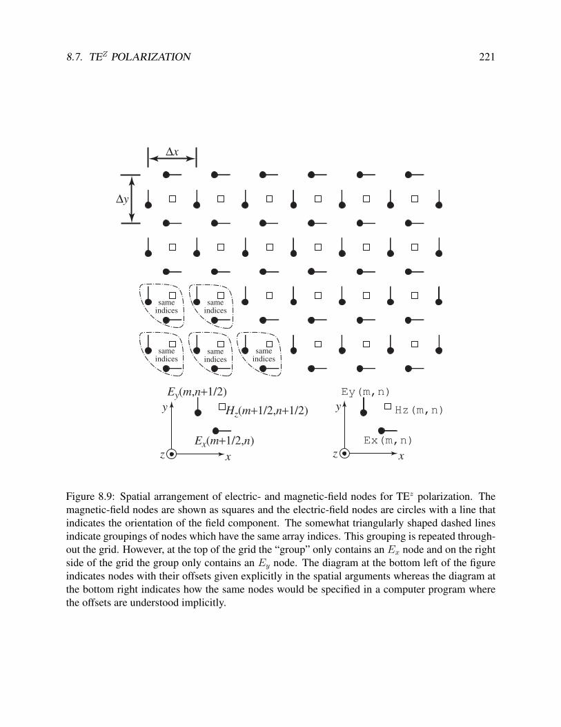
8.7. TEZ POLARIZATION 221
∆x
∆y
sameindices
sameindices
sameindices
sameindices
sameindices
Hz(m,n)y
xz
Ey(m,n)
Ex(m,n)
Hz(m+1/2,n+1/2)
Ey(m,n+1/2)
Ex(m+1/2,n)
y
xz
Figure 8.9: Spatial arrangement of electric- and magnetic-field nodes for TEz polarization. Themagnetic-field nodes are shown as squares and the electric-field nodes are circles with a line thatindicates the orientation of the field component. The somewhat triangularly shaped dashed linesindicate groupings of nodes which have the same array indices. This grouping is repeated through-out the grid. However, at the top of the grid the “group” only contains an Ex node and on the rightside of the grid the group only contains an Ey node. The diagram at the bottom left of the figureindicates nodes with their offsets given explicitly in the spatial arguments whereas the diagram atthe bottom right indicates how the same nodes would be specified in a computer program wherethe offsets are understood implicitly.

222 CHAPTER 8. TWO-DIMENSIONAL FDTD SIMULATIONS
Hz(m+1/2,n+1/2)
Ey(m,n+1/2)
Ex(m+1/2,n)
y
xz
Ez(m,n)
Hy(m+1/2,n)
Hx(m,n+1/2)
sameindices
sameindices
sameindices
sameindices
sameindices
Figure 8.10: Superposition of a TMz and TEz grid. The symbols used for the nodes is as before.The dashed boxes enclose nodes which have the same indices. Although this is nominally identifiedas an M ×N grid, only the Ez array has M ×N nodes.
defining a square with the magnetic field at the center of the square (if the grid is not uniform, thesquare becomes a rectangle). An M × N grid would consist of (M − 1) × (N − 1) completesquares.
The way in which the TEz arrays are dimensioned may seem odd but it is done with an eyetoward having a consistent grid in three dimensions. As an indication of where we will ultimatelyend up, we can overlay a TMz and TEz grid as shown in Fig. 8.10. As will be shown in thediscussion of 3D grids, a 3D grid is essentially layers of TMz and TEz grids which are offset fromeach other in the z direction. The update equations of these offset grids will have to be modified toaccount for variations in the z directions. This modification will provide the coupling between theTMz and TEz grids which is lacking in 2D.
Given the governing equations (8.19)–(8.21) and the arrangement of nodes shown in Fig. 8.9,the Hz update equation is
Hq+ 1
2z
[m+
1
2, n+
1
2
]=
1− σm∆t
2µ
1 + σm∆t
2µ
Hq− 1
2z
[m+
1
2, n+
1
2
]− 1
1 + σm∆t
2ε
(∆t
ε∆x
Eqy
[m+ 1, n+
1
2
]− Eq
y
[m,n+
1
2
]− ∆t
µ∆y
Eqx
[m+
1
2, n+ 1
]− Eq
x
[m+
1
2, n
]).(8.25)
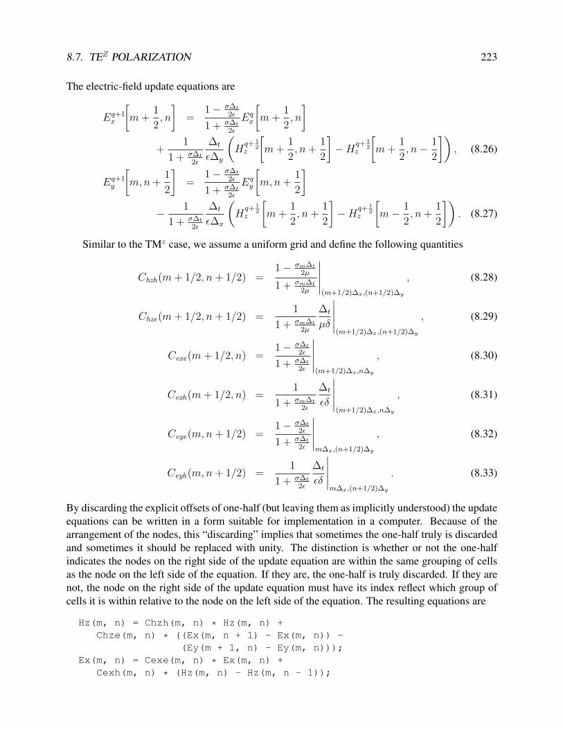
8.7. TEZ POLARIZATION 223
The electric-field update equations are
Eq+1x
[m+
1
2, n
]=
1− σ∆t
2ε
1 + σ∆t
2ε
Eqx
[m+
1
2, n
]+
1
1 + σ∆t
2ε
∆t
ε∆y
(Hq+ 1
2z
[m+
1
2, n+
1
2
]−Hq+ 1
2z
[m+
1
2, n− 1
2
]), (8.26)
Eq+1y
[m,n+
1
2
]=
1− σ∆t
2ε
1 + σ∆t
2ε
Eqy
[m,n+
1
2
]− 1
1 + σ∆t
2ε
∆t
ε∆x
(Hq+ 1
2z
[m+
1
2, n+
1
2
]−Hq+ 1
2z
[m− 1
2, n+
1
2
]). (8.27)
Similar to the TMz case, we assume a uniform grid and define the following quantities
Chzh(m+ 1/2, n+ 1/2) =1− σm∆t
2µ
1 + σm∆t
2µ
∣∣∣∣∣(m+1/2)∆x,(n+1/2)∆y
, (8.28)
Chze(m+ 1/2, n+ 1/2) =1
1 + σm∆t
2µ
∆t
µδ
∣∣∣∣∣(m+1/2)∆x,(n+1/2)∆y
, (8.29)
Cexe(m+ 1/2, n) =1− σ∆t
2ε
1 + σ∆t
2ε
∣∣∣∣∣(m+1/2)∆x,n∆y
, (8.30)
Cexh(m+ 1/2, n) =1
1 + σm∆t
2ε
∆t
εδ
∣∣∣∣∣(m+1/2)∆x,n∆y
, (8.31)
Ceye(m,n+ 1/2) =1− σ∆t
2ε
1 + σ∆t
2ε
∣∣∣∣∣m∆x,(n+1/2)∆y
, (8.32)
Ceyh(m,n+ 1/2) =1
1 + σ∆t
2ε
∆t
εδ
∣∣∣∣∣m∆x,(n+1/2)∆y
. (8.33)
By discarding the explicit offsets of one-half (but leaving them as implicitly understood) the updateequations can be written in a form suitable for implementation in a computer. Because of thearrangement of the nodes, this “discarding” implies that sometimes the one-half truly is discardedand sometimes it should be replaced with unity. The distinction is whether or not the one-halfindicates the nodes on the right side of the update equation are within the same grouping of cellsas the node on the left side of the equation. If they are, the one-half is truly discarded. If they arenot, the node on the right side of the update equation must have its index reflect which group ofcells it is within relative to the node on the left side of the equation. The resulting equations are
Hz(m, n) = Chzh(m, n) * Hz(m, n) +Chze(m, n) * ((Ex(m, n + 1) - Ex(m, n)) -
(Ey(m + 1, n) - Ey(m, n)));Ex(m, n) = Cexe(m, n) * Ex(m, n) +
Cexh(m, n) * (Hz(m, n) - Hz(m, n - 1));

224 CHAPTER 8. TWO-DIMENSIONAL FDTD SIMULATIONS
Total-Field Region
Scattered-Field Region
indices specifyingstart of TF region
indices specifyingend of TF region
Figure 8.11: TFSF boundary in a TEz grid. The rounded boxes indicate the nodes that have aneighboring node on the other side of the boundary and hence have to have their update equationscorrected.
Ey(m, n) = Ceye(m, n) * Ey(m, n) -Ceyh(m, n) * (Hz(m, n) - Hz(m - 1, n));
A TFSF boundary can be incorporated in a TEz grid. Conceptually the implementation is thesame as has been shown in 1D and in the TMz grid. Nodes that are tangential to the boundary willhave a neighboring node on the other side of the boundary. The incident field will have to be eitheradded to or subtracted from that neighboring node to obtain consistent equations. A portion of aTEz grid showing the TFSF boundary is shown in Fig. 8.11. We will specify the size of the TFregion as indicated in the figure. Indices that specify the start of the TF region correspond to thefirst Ex and Ey nodes which are in the TF region. Referring to Figs. 8.4 and 8.10, these indiceswould also correspond to the first Ez node in the TF region. The indices which specify the endof the TF region correspond to Ex and Ey nodes which are actually in the SF region. These twonodes, as shown in Fig. 8.10, are not tangential to the TFSF boundary and hence do to have to becorrected. However, note that the Ez node in the overlain grid that has these indices does lie in theTF region (and does, when dealing with a 3D or TMz grid, have to be corrected to account for thepresence of the boundary).
8.8 PEC’s in TEz and TMz SimulationsWhen modeling a PEC in a TMz grid, if an Ez node falls within the PEC, it is set to zero. Figure8.12 shows a portion of a TMz grid that depicts how Ez would set to zero. The curved boundary

8.8. PEC’S IN TEZ AND TMZ SIMULATIONS 225
Figure 8.12: TMz grid with a PEC object. The PEC is assumed to exist below and to the right ofthe curved boundary. The PEC is realized by setting to zero the Ez nodes that fall within the PEC.The nodes that would be set to zero are surrounded by gray boxes.
is the surface of the PEC and it is assumed that the PEC extends down and to the right of thisboundary. The Ez nodes which would be set to zero are indicated with gray boxes. Although thegoal is to model a continuously varying boundary, the discrete nature of the FDTD grid gives riseto a “staircased” approximation of the surface.
When we say a node is “set to zero” this could mean various things. For example, it may meanthat the field is initially zero and then never updated. It could mean that it is updated, but theupdate coefficients are set to zero. Or, it could even mean that the field is updated with non-zerocoefficients, but then additional code is used to set the field to zero each time-step. The means bywhich a field is set to zero is not particularly important to us right now.
A thin PEC plate can be modeled in a TMz grid by setting to zero nodes along a vertical orhorizontal line. If the physical plate being modeled is not aligned with the grid, one would haveto zero nodes in a manner that approximates the true slope of the plate. Again, this would yield astaircased approximate to the true surface. (One may have to be careful to ensure that there are no“gaps” in the model of a thin PEC that is not aligned with the grid. Fields should only be able toget from one side of the PEC to the other by propagating around the ends of the PEC.)
In a TEz grid, the realization of a PEC is slightly more complicated. For a PEC object which

226 CHAPTER 8. TWO-DIMENSIONAL FDTD SIMULATIONS
Figure 8.13: TEz grid with a PEC object. The PEC is assumed to exist below and to the right of thecurved boundary. The PEC is realized be setting to zero any electric field which has a neighboringHz node within the PEC. The nodes that would be set to zero are surrounded by gray rectangles.
has a specified cross section, one should not merely set to zero the electric-field nodes that fallwithin the boundary of the PEC (as was done in the TMz case). Instead, one should consider thePEC as consisting of a collection of patches of metal. If an Hz node falls within the PEC, then foursurrounding electric-field nodes should be set to zero. Thus, if an Hz node is in the PEC we fill thesquare surrounding that node with PEC and this causes the four surrounding electric field nodes tobe zero. The TEz representation of a PEC object is depicted in Fig. 8.13. The object is the sameas shown in Fig. 8.12. In both figures the curved boundary is a portion of a circle that is center onwhat would correspond to the location of an Ez node (regardless of whether or not an Ez node isactually present). The nodes that are set to zero are enclosed in gray rectangles.
A horizontal PEC plate would be implemented by zeroing a horizontal line of Ex nodes whilea vertical plate would be realized by zeroing a vertical line of Ey nodes. A tilted plate would berealized as a combination of zeroed Ex and Ey nodes.
For both TEz and TMz grids, all the magnetic fields are updated in the usual way. Magneticfields are oblivious to the presence of PEC’s.

8.9. TEZ EXAMPLE 227
8.9 TEz ExampleIn this section we present the computer code to model a circular PEC scatterer in a TEz grid. Thescatterer is illuminated by a pulsed plane wave that is introduced via a TFSF boundary. We willuse a grid that is nominally 92 by 82 (keeping in mind that for TEz polarization none of the fieldarrays will actually have these dimensions). The code is organized in essentially the same way aswas the TMz code presented in Sec. 8.6.
The PEC scatterer is assumed to have a radius of 12 cells and be centered on an Hz node. Theindices of the center are (45, 40). The PEC is realized by checking if an Hz node is within thecircle (specifically, if the distance from the center to the node is less than the radius). As we willsee, if an Hz is within the circle, the four surrounding electric-field nodes are set to zero by settingthe corresponding update coefficients to zero.
Program 8.17 contains the main() function. Other than the difference of one header file, thisprogram is identical to the TMz code presented in Program 8.12. However, despite similar names,the functions that are called here differ from those used by Program 8.12—different files are linkedtogether for the different simulations.
Program 8.17 tezdemo.c The main() function for a simulation involving a TEz grid.
1 /* TEz simulation with a TFSF boundary and a second-order ABC. */2
3 #include "fdtd-alloc1.h"4 #include "fdtd-macro-tez.h"5 #include "fdtd-proto2.h"6
7 int main()8 9 Grid *g;
10
11 ALLOC_1D(g, 1, Grid); // allocate memory for grid12 gridInit(g); // initialize 2D grid13
14 abcInit(g); // initialize ABC15 tfsfInit(g); // initialize TFSF boundary16 snapshotInit2d(g); // initialize snapshots17
18 /* do time stepping */19 for (Time = 0; Time < MaxTime; Time++) 20 updateH2d(g); // update magnetic fields21 tfsfUpdate(g); // apply TFSF boundary22 updateE2d(g); // update electric fields23 abc(g); // apply ABC24 snapshot2d(g); // take a snapshot (if appropriate)25 // end of time-stepping26
27 return 0;

228 CHAPTER 8. TWO-DIMENSIONAL FDTD SIMULATIONS
28
The code to construct the TEz grid is shown in Program 8.18, i.e., the code to set the elementsof the Grid pointer g. The simulation is run at the Courant limit of 1/
√2 as shown in line 16.
Between lines 31 and 41 the update coefficients for all the electric field nodes are set to that of freespace. Then, starting at line 49, each Hz node is checked to see if it is within the PEC scatterer. Ifit is, the coefficients for the surrounding nodes are set to zero. Starting at line 71 all the magnetic-field coefficients are set to that of free space. There is no need to change these coefficients toaccount for the PEC—the PEC is realized solely by dictating the behavior of the electric field.
Program 8.18 gridtezpec.c Function to initialize a TEz grid. A circular PEC scatterer ispresent.
1 #include "fdtd-macro-tez.h"2 #include "fdtd-alloc1.h"3 #include <math.h>4
5 void gridInit(Grid *g) 6 double imp0 = 377.0;7 int mm, nn;8
9 /* terms for the PEC scatterer */10 double rad, r2, xLocation, yLocation, xCenter, yCenter;11
12 Type = teZGrid;13 SizeX = 92; // size of domain14 SizeY = 82;15 MaxTime = 300; // duration of simulation16 Cdtds = 1.0 / sqrt(2.0); // Courant number17
18 ALLOC_2D(g->hz, SizeX - 1, SizeY - 1, double);19 ALLOC_2D(g->chzh, SizeX - 1, SizeY - 1, double);20 ALLOC_2D(g->chze, SizeX - 1, SizeY - 1, double);21
22 ALLOC_2D(g->ex, SizeX - 1, SizeY, double);23 ALLOC_2D(g->cexh, SizeX - 1, SizeY, double);24 ALLOC_2D(g->cexe, SizeX - 1, SizeY, double);25
26 ALLOC_2D(g->ey, SizeX, SizeY - 1, double);27 ALLOC_2D(g->ceye, SizeX, SizeY - 1, double);28 ALLOC_2D(g->ceyh, SizeX, SizeY - 1, double);29
30 /* set electric-field update coefficients */31 for (mm = 0; mm < SizeX - 1; mm++)32 for (nn = 0; nn < SizeY; nn++)

8.9. TEZ EXAMPLE 229
33 Cexe(mm, nn) = 1.0;34 Cexh(mm, nn) = Cdtds * imp0;35 36
37 for (mm = 0; mm < SizeX; mm++)38 for (nn = 0; nn < SizeY - 1; nn++) 39 Ceye(mm, nn) = 1.0;40 Ceyh(mm, nn) = Cdtds * imp0;41 42
43 /* Set to zero nodes associated with PEC scatterer.44 * Circular scatterer assumed centered on Hz node45 * at (xCenter, yCenter). If an Hz node is less than46 * the radius away from this node, set to zero the47 * four electric fields that surround that node.48 */49 rad = 12; // radius of circle50 xCenter = SizeX / 2;51 yCenter = SizeY / 2;52 r2 = rad * rad; // square of radius53 for (mm = 1; mm < SizeX - 1; mm++) 54 xLocation = mm - xCenter;55 for (nn = 1; nn < SizeY - 1; nn++) 56 yLocation = nn - yCenter;57 if (xLocation * xLocation + yLocation * yLocation < r2) 58 Cexe(mm, nn) = 0.0;59 Cexh(mm, nn) = 0.0;60 Cexe(mm, nn + 1) = 0.0;61 Cexh(mm, nn + 1) = 0.0;62 Ceye(mm + 1, nn) = 0.0;63 Ceyh(mm + 1, nn) = 0.0;64 Ceye(mm, nn) = 0.0;65 Ceyh(mm, nn) = 0.0;66 67 68 69
70 /* set magnetic-field update coefficients */71 for (mm = 0; mm < SizeX - 1; mm++)72 for (nn = 0; nn < SizeY - 1; nn++) 73 Chzh(mm, nn) = 1.0;74 Chze(mm, nn) = Cdtds / imp0;75 76
77 return;78

230 CHAPTER 8. TWO-DIMENSIONAL FDTD SIMULATIONS
The header file fdtd-macro-tez.h that defines the macros used in the TEz simulations isshown in Program 8.19. The header files that define the function prototypes (fdtd-proto2.h),the allocation macros (fdtd-alloc1.h), and the Grid structure (fdtd-grid1.h) are un-changed from before and hence are not repeated here (refer to Programs 8.13, 8.4, and 8.3, respec-tively).
Program 8.19 fdtd-macro-tez.h Macros used for TEz grids.
1 #ifndef _FDTD_MACRO_TEZ_H2 #define _FDTD_MACRO_TEZ_H3
4 #include "fdtd-grid1.h"5
6 /* macros that permit the "Grid" to be specified */7 /* one-dimensional grid */8 #define Hz1G(G, M) G->hz[M]9 #define Chzh1G(G, M) G->chzh[M]
10 #define Chze1G(G, M) G->chze[M]11
12 #define Ey1G(G, M) G->ey[M]13 #define Ceye1G(G, M) G->ceye[M]14 #define Ceyh1G(G, M) G->ceyh[M]15
16 /* TEz grid */17 #define HzG(G, M, N) G->hz[(M) * (SizeYG(G) - 1) + (N)]18 #define ChzhG(G, M, N) G->chzh[(M) * (SizeYG(G) - 1) + (N)]19 #define ChzeG(G, M, N) G->chze[(M) * (SizeYG(G) - 1) + (N)]20
21 #define ExG(G, M, N) G->ex[(M) * SizeYG(G) + (N)]22 #define CexeG(G, M, N) G->cexe[(M) * SizeYG(G) + (N)]23 #define CexhG(G, M, N) G->cexh[(M) * SizeYG(G) + (N)]24
25 #define EyG(G, M, N) G->ey[(M) * (SizeYG(G) - 1) + (N)]26 #define CeyeG(G, M, N) G->ceye[(M) * (SizeYG(G) - 1) + (N)]27 #define CeyhG(G, M, N) G->ceyh[(M) * (SizeYG(G) - 1) + (N)]28
29 #define SizeXG(G) G->sizeX30 #define SizeYG(G) G->sizeY31 #define SizeZG(G) G->sizeZ32 #define TimeG(G) G->time33 #define MaxTimeG(G) G->maxTime34 #define CdtdsG(G) G->cdtds35 #define TypeG(G) G->type36
37 /* macros that assume the "Grid" is "g" */38 /* one-dimensional grid */

8.9. TEZ EXAMPLE 231
39 #define Hz1(M) Hz1G(g, M)40 #define Chzh1(M) Chzh1G(g, M)41 #define Chze1(M) Chze1G(g, M)42
43 #define Ey1(M) Ey1G(g, M)44 #define Ceye1(M) Ceye1G(g, M)45 #define Ceyh1(M) Ceyh1G(g, M)46
47 /* TEz grid */48 #define Hz(M, N) HzG(g, M, N)49 #define Chzh(M, N) ChzhG(g, M, N)50 #define Chze(M, N) ChzeG(g, M, N)51
52 #define Ex(M, N) ExG(g, M, N)53 #define Cexh(M, N) CexhG(g, M, N)54 #define Cexe(M, N) CexeG(g, M, N)55
56 #define Ey(M, N) EyG(g, M, N)57 #define Ceye(M, N) CeyeG(g, M, N)58 #define Ceyh(M, N) CeyhG(g, M, N)59
60 #define SizeX SizeXG(g)61 #define SizeY SizeYG(g)62 #define SizeZ SizeZG(g)63 #define Time TimeG(g)64 #define MaxTime MaxTimeG(g)65 #define Cdtds CdtdsG(g)66 #define Type TypeG(g)67
68 #endif /* matches #ifndef _FDTD_MACRO_TEZ_H */
The functions to update the fields are shown in Program 8.20. These functions can updatefields in either one- or two-dimensional grid. If the grid type is oneDGrid, here it is assumedthe non-zero fields are Ey and Hz. If that is not the case, it is assume the grid is a TEz grid withnon-zero fields Ex, Ey, and Hz. As has been the case in the past the electric field updates, startingat line 37, update all the nodes except the nodes at the edge of the grid. However, since all themagnetic-field nodes have all their neighbors, as shown starting on line 15, all the magnetic-fieldnodes in the grid are updated.
Program 8.20 updatetez.c: Functions to update fields in a TEz grid.
1 #include "fdtd-macro-tez.h"2
3 /* update magnetic field */4 void updateH2d(Grid *g)

232 CHAPTER 8. TWO-DIMENSIONAL FDTD SIMULATIONS
5 int mm, nn;6
7 if (Type == oneDGrid) 8
9 for (mm = 0; mm < SizeX - 1; mm++)10 Hz1(mm) = Chzh1(mm) * Hz1(mm)11 - Chze1(mm) * (Ey1(mm + 1) - Ey1(mm));12
13 else 14
15 for (mm = 0; mm < SizeX - 1; mm++)16 for (nn = 0; nn < SizeY - 1; nn++)17 Hz(mm, nn) = Chzh(mm, nn) * Hz(mm, nn) +18 Chze(mm, nn) * ((Ex(mm, nn + 1) - Ex(mm, nn))19 - (Ey(mm + 1, nn) - Ey(mm, nn)));20 21
22 return;23 24
25 /* update electric field */26 void updateE2d(Grid *g) 27 int mm, nn;28
29 if (Type == oneDGrid) 30
31 for (mm = 1; mm < SizeX - 1; mm++)32 Ey1(mm) = Ceye1(mm) * Ey1(mm)33 - Ceyh1(mm) * (Hz1(mm) - Hz1(mm - 1));34
35 else 36
37 for (mm = 0; mm < SizeX - 1; mm++)38 for (nn = 1; nn < SizeY - 1; nn++)39 Ex(mm, nn) = Cexe(mm, nn) * Ex(mm, nn) +40 Cexh(mm, nn) * (Hz(mm, nn) - Hz(mm, nn - 1));41
42 for (mm = 1; mm < SizeX - 1; mm++)43 for (nn = 0; nn < SizeY - 1; nn++)44 Ey(mm, nn) = Ceye(mm, nn) * Ey(mm, nn) -45 Ceyh(mm, nn) * (Hz(mm, nn) - Hz(mm - 1, nn));46 47
48 return;49
The second-order absorbing boundary condition is realized with the code in the file abctez.c

8.9. TEZ EXAMPLE 233
which is shown in Program 8.21. Because of the way the grid is constructed, the ABC is appliedto Ey nodes along the left and right side of the computational domain and to Ex nodes along thetop and bottom.
Program 8.21 abctez.c: Contents of file that implements the second-order absorbing bound-ary condition for the TEz grid.
1 /* Second-order ABC for TEz grid. */2 #include <math.h>3 #include "fdtd-alloc1.h"4 #include "fdtd-macro-tez.h"5
6 /* Define macros for arrays that store the previous values of the7 * fields. For each one of these arrays the three arguments are as8 * follows:9 *
10 * first argument: spatial displacement from the boundary11 * second argument: displacement back in time12 * third argument: distance from either the bottom (if EyLeft or13 * EyRight) or left (if ExTop or ExBottom) side14 * of grid15 *16 */17 #define EyLeft(M, Q, N) eyLeft[(N) * 6 + (Q) * 3 + (M)]18 #define EyRight(M, Q, N) eyRight[(N) * 6 + (Q) * 3 + (M)]19 #define ExTop(N, Q, M) exTop[(M) * 6 + (Q) * 3 + (N)]20 #define ExBottom(N, Q, M) exBottom[(M) * 6 + (Q) * 3 + (N)]21
22 static int initDone = 0;23 static double coef0, coef1, coef2;24 static double *eyLeft, *eyRight, *exTop, *exBottom;25
26 void abcInit(Grid *g) 27 double temp1, temp2;28
29 initDone = 1;30
31 /* allocate memory for ABC arrays */32 ALLOC_1D(eyLeft, (SizeY - 1) * 6, double);33 ALLOC_1D(eyRight, (SizeY - 1) * 6, double);34 ALLOC_1D(exTop, (SizeX - 1) * 6, double);35 ALLOC_1D(exBottom, (SizeX - 1) * 6, double);36
37 /* calculate ABC coefficients */38 temp1 = sqrt(Cexh(0, 0) * Chze(0, 0));39 temp2 = 1.0 / temp1 + 2.0 + temp1;

234 CHAPTER 8. TWO-DIMENSIONAL FDTD SIMULATIONS
40 coef0 = -(1.0 / temp1 - 2.0 + temp1) / temp2;41 coef1 = -2.0 * (temp1 - 1.0 / temp1) / temp2;42 coef2 = 4.0 * (temp1 + 1.0 / temp1) / temp2;43
44 return;45 46
47 void abc(Grid *g)48 49 int mm, nn;50
51 /* ABC at left side of grid */52 for (nn = 0; nn < SizeY - 1; nn++) 53 Ey(0, nn) = coef0 * (Ey(2, nn) + EyLeft(0, 1, nn))54 + coef1 * (EyLeft(0, 0, nn) + EyLeft(2, 0, nn)55 - Ey(1, nn) - EyLeft(1, 1, nn))56 + coef2 * EyLeft(1, 0, nn) - EyLeft(2, 1, nn);57
58 /* memorize old fields */59 for (mm = 0; mm < 3; mm++) 60 EyLeft(mm, 1, nn) = EyLeft(mm, 0, nn);61 EyLeft(mm, 0, nn) = Ey(mm, nn);62 63 64
65 /* ABC at right side of grid */66 for (nn = 0; nn < SizeY - 1; nn++) 67 Ey(SizeX - 1, nn) = coef0 * (Ey(SizeX - 3, nn) + EyRight(0, 1, nn))68 + coef1 * (EyRight(0, 0, nn) + EyRight(2, 0, nn)69 - Ey(SizeX - 2, nn) - EyRight(1, 1, nn))70 + coef2 * EyRight(1, 0, nn) - EyRight(2, 1, nn);71
72 /* memorize old fields */73 for (mm = 0; mm < 3; mm++) 74 EyRight(mm, 1, nn) = EyRight(mm, 0, nn);75 EyRight(mm, 0, nn) = Ey(SizeX - 1 - mm, nn);76 77 78
79 /* ABC at bottom of grid */80 for (mm = 0; mm < SizeX - 1; mm++) 81 Ex(mm, 0) = coef0 * (Ex(mm, 2) + ExBottom(0, 1, mm))82 + coef1 * (ExBottom(0, 0, mm) + ExBottom(2, 0, mm)83 - Ex(mm, 1) - ExBottom(1, 1, mm))84 + coef2 * ExBottom(1, 0, mm) - ExBottom(2, 1, mm);85
86 /* memorize old fields */

8.9. TEZ EXAMPLE 235
87 for (nn = 0; nn < 3; nn++) 88 ExBottom(nn, 1, mm) = ExBottom(nn, 0, mm);89 ExBottom(nn, 0, mm) = Ex(mm, nn);90 91 92
93 /* ABC at top of grid */94 for (mm = 0; mm < SizeX - 1; mm++) 95 Ex(mm, SizeY - 1) = coef0 * (Ex(mm, SizeY - 3) + ExTop(0, 1, mm))96 + coef1 * (ExTop(0, 0, mm) + ExTop(2, 0, mm)97 - Ex(mm, SizeY - 2) - ExTop(1, 1, mm))98 + coef2 * ExTop(1, 0, mm) - ExTop(2, 1, mm);99
100 /* memorize old fields */101 for (nn = 0; nn < 3; nn++) 102 ExTop(nn, 1, mm) = ExTop(nn, 0, mm);103 ExTop(nn, 0, mm) = Ex(mm, SizeY - 1-nn);104 105 106
107 return;108
The contents of the file tfsftez.c are shown in Program 8.22. This closely follows theTFSF code that was used for the TMz grid. Again, a 1D auxiliary grid is used to describe theincident field. The 1D grid is available via in the Grid pointer g1 which is only visible to thefunctions in this file. Space for the structure is allocated in line 16. In the following line thecontents of the 2D structure are copied to the 1D structure. This is done to set the size of the gridand the Courant number. Then, in line 18, the function gridInit1d() is called to complete theinitialization of the 1D grid.
The function tfsfUpdate(), which starts on line 31, is called once per time-step. Afterensuring that the initialization function has been called, the magnetic fields adjacent to the TFSFboundary are corrected. Following this, as shown starting on line 52, the magnetic field in the 1Dgrid is updated, then the 1D electric field is updated, then the source function is applied to the firstnode in the 1D grid, and finally the time-step of the 1D grid is incremented. Starting on line 58,the electric fields in the 2D grid adjacent to the TFSF boundary are corrected.
The header file ezinctez.h differs from ezinc.h used in the TMz code only in that it in-cludes fdtd-macro-tez.h instead of fdtd-macro-tmz.h. Hence it is not shown here noris the code used to realize the source function which is a Ricker wavelet (which is also essentiallyunchanged from before).
Program 8.22 tfsftez.c: Implementation of a TFSF boundary for a TEz grid. The incidentfield propagates in the x direction and an auxiliary 1D grid is used to compute the incident field.

236 CHAPTER 8. TWO-DIMENSIONAL FDTD SIMULATIONS
1 /* TFSF implementation for a TEz grid. */2
3 #include <string.h> // for memcpy4 #include "fdtd-macro-tez.h"5 #include "fdtd-proto2.h"6 #include "fdtd-alloc1.h"7 #include "ezinctez.h"8
9 static int firstX = 0, firstY, // indices for first point in TF region10 lastX, lastY; // indices for last point in TF region11
12 static Grid *g1; // 1D auxilliary grid13
14 void tfsfInit(Grid *g) 15
16 ALLOC_1D(g1, 1, Grid); // allocate memory for 1D Grid17 memcpy(g1, g, sizeof(Grid)); // copy information from 2D array18 gridInit1d(g1); // initialize 1d grid19
20 printf("Grid is %d by %d cell.\n", SizeX, SizeY);21 printf("Enter indices for first point in TF region: ");22 scanf(" %d %d", &firstX, &firstY);23 printf("Enter indices for last point in TF region: ");24 scanf(" %d %d", &lastX, &lastY);25
26 ezIncInit(g); // initialize source function27
28 return;29 30
31 void tfsfUpdate(Grid *g) 32 int mm, nn;33
34 // check if tfsfInit() has been called35 if (firstX <= 0) 36 fprintf(stderr,37 "tfsfUpdate: tfsfInit must be called before tfsfUpdate.\n"38 " Boundary location must be set to positive value.\n");39 exit(-1);40 41
42 // correct Hz along left edge43 mm = firstX - 1;44 for (nn = firstY; nn < lastY; nn++)45 Hz(mm, nn) += Chze(mm, nn) * Ey1G(g1, mm + 1);46
47 // correct Hz along right edge

8.9. TEZ EXAMPLE 237
48 mm = lastX;49 for (nn = firstY; nn < lastY; nn++)50 Hz(mm, nn) -= Chze(mm, nn) * Ey1G(g1, mm);51
52 updateH2d(g1); // update 1D magnetic field53 updateE2d(g1); // update 1D electric field54 Ey1G(g1, 0) = ezInc(TimeG(g1), 0.0); // set source node55 TimeG(g1)++; // increment time in 1D grid56
57 // correct Ex along the bottom58 nn = firstY;59 for (mm = firstX; mm < lastX; mm++)60 Ex(mm, nn) -= Cexh(mm, nn) * Hz1G(g1, mm);61
62 // correct Ex along the top63 nn = lastY;64 for (mm = firstX; mm < lastX; mm++)65 Ex(mm, nn) += Cexh(mm, nn) * Hz1G(g1, mm);66
67 // correct Ey field along left edge68 mm = firstX;69 for (nn = firstY; nn < lastY; nn++)70 Ey(mm, nn) += Ceyh(mm, nn) * Hz1G(g1, mm - 1);71
72 // correct Ey field along right edge73 mm = lastX;74 for (nn = firstY; nn < lastY; nn++)75 Ey(mm, nn) -= Ceyh(mm, nn) * Hz1G(g1, mm);76
77 // no need to correct Ex along top and bottom since78 // incident Ex is zero79
80 return;81
The function to initialize the 1D auxiliary grid is shown in Program 8.23. As was the case forthe TMz case, the grid is terminated on the right with a lossy layer that is 20 cells wide. The restof the grid corresponds to free space. (The first node in the grid is the hard-wired source node andhence the left side of the grid does not need to be terminated.)
Program 8.23 grid1dhz.c: Initialization function used for the 1D auxiliary grid for the TEz
TFSF boundary.
1 /* Create a 1D grid suitable for an auxilliary grid used as part of2 * the implementation of a TFSF boundary in a TEz simulations. */

238 CHAPTER 8. TWO-DIMENSIONAL FDTD SIMULATIONS
3
4 #include <math.h>5 #include "fdtd-macro-tez.h"6 #include "fdtd-alloc1.h"7
8 #define NLOSS 20 // number of lossy cells at end of 1D grid9 #define MAX_LOSS 0.35 // maximum loss factor in lossy layer
10
11 void gridInit1d(Grid *g) 12 double imp0 = 377.0, depthInLayer = 0.0, lossFactor;13 int mm;14
15 SizeX += NLOSS; // size of domain16 Type = oneDGrid; // set grid type17
18 ALLOC_1D(g->hz, SizeX - 1, double);19 ALLOC_1D(g->chzh, SizeX - 1, double);20 ALLOC_1D(g->chze, SizeX - 1, double);21 ALLOC_1D(g->ey, SizeX, double);22 ALLOC_1D(g->ceye, SizeX, double);23 ALLOC_1D(g->ceyh, SizeX, double);24
25 /* set electric-field update coefficients */26 for (mm = 0; mm < SizeX - 1; mm++) 27 if (mm < SizeX - 1 - NLOSS) 28 Ceye1(mm) = 1.0;29 Ceyh1(mm) = Cdtds * imp0;30 Chzh1(mm) = 1.0;31 Chze1(mm) = Cdtds / imp0;32 else 33 depthInLayer += 0.5;34 lossFactor = MAX_LOSS * pow(depthInLayer / NLOSS, 2);35 Ceye1(mm) = (1.0 - lossFactor) / (1.0 + lossFactor);36 Ceyh1(mm) = Cdtds * imp0 / (1.0 + lossFactor);37 depthInLayer += 0.5;38 lossFactor = MAX_LOSS * pow(depthInLayer / NLOSS, 2);39 Chzh1(mm) = (1.0 - lossFactor) / (1.0 + lossFactor);40 Chze1(mm) = Cdtds / imp0 / (1.0 + lossFactor);41 42 43
44 return;45
Figure 8.14 shows snapshots of the magnetic field throughout the computational domain atthree different times. The snapshot in Fig. 8.14(a) was taken after 60 time steps. The leading edgeof the incident pulse has just started to interact with the scatterer. No scattered fields are evident

8.9. TEZ EXAMPLE 239
in the SF region. The snapshot in Fig. 8.14(b) was taken after 100 time steps. The entire scattereris now visible and scattered fields have just started to enter the SF region. The final snapshot wastaken after 140 time steps.
To obtain these snapshots, the snapshot code of Program 8.11 has to be slightly modified. Sincewe are now interested in obtaining Hz instead of Ez, the limits of the for-loops starting in line 68of Program 8.11 would have to be changed to that which pertain to the Hz array. Furthermore,one would have to change Ez(mm, nn) in line 70 to Hz(mm, nn). Because these changes areminor, the modified version of the program is not shown.

240 CHAPTER 8. TWO-DIMENSIONAL FDTD SIMULATIONS
(a)
(b)
(c)
Figure 8.14: Pulsed TEz illumination of a circular scatter. Display of the Hz field at time-steps (a)60, (b) 100 and (c) 140. The field has been normalized by 1/377 (i.e., the characteristic impedanceof free space) and is shown with three decades of logarithmic scaling. The incident field is a Rickerwavelet discretized such that there are 30 points per wavelength at the most energetic frequency.

Chapter 9
Three-Dimensional FDTD
9.1 IntroductionWith an understanding of the FDTD implementation of TEz and TMz grids, the additional stepsneeded to implement a three-dimensional (3D) grid are almost trivial. A 3D grid can be viewedas stacked layers of TEz and TMz grids which are offset a half spatial step in the z direction. Theupdate equations for the Hz and Ez nodes are nearly identical to those which have been givenalready—the only difference is an additional index to specify the z location. The update equationsfor the other field components require slight changes to account for variations in the z direction(i.e., in the governing equations the partial derivative with respect to z is no longer zero).
We begin this chapter by discussing the implementation of 3D arrays in C. This is followedby details concerning the arrangement of nodes in 3D and the associated update equations. Thechapter concludes with the code for an incremental dipole in a homogeneous space.
9.2 3D Arrays in CFor fields in a 3D space, it is, of course, natural to specify the location of a node using three indicesrepresenting the displacement in the x, y, and z directions. However, as was done for 2D grids, wewill use a macro to translate the given indices into an offset into a 1D array. The memory associatedwith the 1D array will be allocated dynamically and the amount of memory will be precisely whatis needed to store all the elements of the 3D “array.” (We will refer to the macro as a 3D arraysince, other than the cleaner specification of the indices, its use in the code is indistinguishablefrom a traditional 3D array.)
For 3D arrays, incrementing the third index by one changes the variable being specified tothe next consecutive variable in memory. Thinking of the third index as corresponding to the zdirection, this implies that nodes that are adjacent to each other in the z direction are also adjacentto each other in memory. On the other hand, when the first or second index is incremented by one,that will not correspond to the next variable in memory. When the second index is incremented,one must move forward in memory an amount corresponding to the number of variables in thethird dimension. For example, if the array size in the third dimension was 32 elements, then
Lecture notes by John Schneider. fdtd-3d.tex
241

242 CHAPTER 9. THREE-DIMENSIONAL FDTD
Ez(0,0,0)
Ez(1,0,0)
Ez(2,0,0)
Ez(0,1,0)
Ez(1,1,0)
Ez(2,1,0)
Ez(0,2,0)
Ez(1,2,0)
Ez(2,2,0)
Ez(0,3,0)
Ez(1,3,0)
Ez(2,3,0)
Ez(0,0,1)
Ez(1,0,1)
Ez(2,0,1)
Ez(0,1,1)
Ez(1,1,1)
Ez(2,1,1)
Ez(0,2,1)
Ez(1,2,1)
Ez(2,2,1)
Ez(0,3,1)
Ez(1,3,1)
Ez(2,3,1)
Ez(0,0,2)
Ez(1,0,2)
Ez(2,0,2)
Ez(0,1,2)
Ez(1,1,2)
Ez(2,1,2)
Ez(0,2,2)
Ez(1,2,2)
Ez(2,2,2)
Ez(0,3,2)
Ez(1,3,2)
Ez(2,3,2)
n=0
m=0
n=3n=2n=1
m=1
m=2
p=0
p=2
p=1
yx
z
Figure 9.1: Depiction of elements of an array with dimensions 3×4×3 in the x, y, and z directions,respectively. The indices m, n, and p, are used to specify the x, y, and z locations, respectively.The element at the “origin” has indices (0, 0, 0) and is shown in the upper left corner of the bottomplane.
incrementing the second index by one would require that the offset in memory be advanced by32. This is the same as in the 2D case where we can think of the size of the third dimension ascorresponding to the number of columns (or, said another way, the number of elements in a row).
When the first index is incremented by one, the offset in memory must account for the arraysize in both the second and third dimension. To illustrate this, consider Fig. 9.1 which shows theelements of the 3D array Ez. The array is 3×4×3, corresponding to the dimensions in the x, y andz directions. In reality, these elements will map to elements of a 1D array called ezwhich is shownin 9.2. Since ez is a 1D array, it takes a single index (or offset). Note that if one holds the m and nindices fixed (corresponding to the x and y directions) but increments the p index (correspondingto a movement in the z direction), the index of ez changes by one. However, if m and p are heldfixed and n is incremented by one, the index of ez changed by 3 which correspond to the numberof elements in the z directions. Finally, if n and p are held fixed but m is incremented by one,the index of ez changed by 12 which is the product of the dimensions in the y and z directions.Three-dimensional arrays can be thought of as a collection of 2D arrays. For the way in whichwe perform the indexing, the 2D arrays correspond to constant-x planes. Each of these 2D arraysmust be large enough to hold the product of the number of elements along the y and z directions.
The construct we use for 3D arrays largely parallels that which was used for 2D arrays. Theallocation macro ALLOC 3D() is shown in Fragment 9.1. The only difference between this andthe allocation macros shown previously is the addition of another argument to specify the size ofthe array in the third dimension (this is the argument NUMZ). This dimension is multiplied by theother two dimensions and used as the first argument of calloc().

9.2. 3D ARRAYS IN C 243
ez[0]
ez[12]
ez[24]
ez[3]
ez[15]
ez[27]
ez[6]
ez[18]
ez[30]
ez[9]
ez[21]
ez[33]
ez[1]
ez[13]
ez[25]
ez[4]
ez[16]
ez[28]
ez[7]
ez[19]
ez[31]
ez[10]
ez[22]
ez[34]
ez[2]
ez[14]
ez[26]
ez[5]
ez[17]
ez[29]
ez[8]
ez[20]
ez[32]
ez[11]
ez[23]
ez[35]
n=0
m=0
n=3n=2n=1
m=1
m=2
p=0
p=2
p=1
yx
z
Figure 9.2: The 1D array ez is used to store the elements of Ez. The three indices for eachelements of Ez shown in Fig. 9.1 map to the single index shown here.
Fragment 9.1 Macro for allocating memory for a 3D array.
1 #define ALLOC_3D(PNTR, NUMX, NUMY, NUMZ, TYPE) \2 PNTR = (TYPE *)calloc((NUMX) * (NUMY) * (NUMZ), sizeof(TYPE)); \3 if (!PNTR) \4 perror("ALLOC_3D"); \5 fprintf(stderr, \6 "Allocation failed for " #PNTR ". Terminating...\n"); \7 exit(-1); \8
To illustrate the construction and use of a 3D array, the code in Fragment 9.2 shows howone could create a 6 × 7 × 8 array. In this example the array dimensions are set in #define-statements in lines 1–3. Line 5 provides the macro Ez() which takes three (dummy) arguments.The preprocessor will replace all occurrences of Ez() with the expression involving ez[] shownat the right. The pointer ez is defined in line 6 and initially at run-time does not have any memoryassociated with it. However, after line 9 has executed ez will point to a block of memory that issufficient to hold all the elements of the array and, at this point, ez can be treated as a 1D array (butwe never use ez directly in the code—instead, we use the macro Ez() to access array elements).The nested for-loops starting at line 11 merely set each element equal to the product of the indicesfor that element. Note that this order of nesting is the one that should be used in practice: theinner-most loop should be over the z index and the outer-most loop should be over the x index.(This order helps minimize page faults and hence maximize performance.)

244 CHAPTER 9. THREE-DIMENSIONAL FDTD
Fragment 9.2 Demonstration of the construction and manipulation of a 6× 7× 8 array.
1 #define num_rows 82 #define num_columns 73 #define num_planes 64
5 #define Ez(M, N, P) ez[((M) * num_columns + (N)) * num_rows + (P)]
...
6 double *ez;7 int m, n, p;8
9 ALLOC_3D(ez, num_planes, num_columns, num_rows, double);10
11 for (m = 0; m < num_planes; m++)12 for (n = 0; n < num_columns; n++)13 for (p = 0; p < num_rows; p++)14 Ez(m, n, p) = m * n * p;
9.3 Governing Equations and the 3D GridAs has been the case previously, Ampere’s and Faraday’s laws are the relevant governing equationsin constructing the FDTD algorithm. These equations are
−σmH− µ∂H
∂t= ∇× E =
∣∣∣∣∣∣ax ay az∂∂x
∂∂y
∂∂z
Ex Ey Ez
∣∣∣∣∣∣ , (9.1)
σE + ε∂E
∂t= ∇×H =
∣∣∣∣∣∣ax ay az∂∂x
∂∂x
∂∂z
Hx Hy Hz
∣∣∣∣∣∣ . (9.2)
The components of these equations, when approximated by finite-differences at the appropriatepoints in space-time, yield the discretized update equations.
The necessary arrangement of nodes is show in Fig. 9.3. This grouping of six nodes can beconsidered the fundamental building block of a 3D grid. The following notation is used:
Hx(x, y, z, t) = Hx(m∆x, n∆y, p∆z, q∆t) = Hqx[m,n, p] , (9.3)
Hy(x, y, z, t) = Hy(m∆x, n∆y, p∆z, q∆t) = Hqy [m,n, p] , (9.4)
Hz(x, y, z, t) = Hz(m∆x, n∆y, p∆z, q∆t) = Hqz [m,n, p] , (9.5)
Ex(x, y, z, t) = Ex(m∆x, n∆y, p∆z, q∆t) = Eqx[m,n, p] , (9.6)
Ey(x, y, z, t) = Ey(m∆x, n∆y, p∆z, q∆t) = Eqy [m,n, p] , (9.7)
Ez(x, y, z, t) = Ez(m∆x, n∆y, p∆z, q∆t) = Eqz [m,n, p] . (9.8)

9.3. GOVERNING EQUATIONS AND THE 3D GRID 245
Hz(m+1/2,n+1/2,p)
Ey(m,n+1/2,p)
Ex(m+1/2,n,p)
Hy(m+1/2,n,p+1/2)Hx(m,n+1/2,p+1/2)
y
x
z
Ez(m,n,p+1/2)
Figure 9.3: Arrangement of nodes in three dimensions. In a computer program all these nodeswould have the same m, n, and p indices (the one-halves would be discarded from the equations—the offset would be understood). Electric-field nodes are displaced a half step in the direction inwhich they point while magnetic-field nodes are displaced a half step in the two directions theydo not point. It is also implicitly understood that the electric- and magnetic-field nodes are offsetfrom each other a half step in time.
In Fig. 9.3 the temporal location of the nodes is not specified. It is assumed the electric-fieldnodes exist at integer multiples of the time step and the magnetic-field nodes exists one-half ofa temporal step away from the electric field nodes. As we will see when we implement the 3Dalgorithm in a computer program, the halves are suppressed and these six nodes will all have thesame indices. Note that, for any given set of indices the electric-field nodes are displaced a halfstep in the direction in which they point while magnetic-field nodes are displaced a half step in thetwo directions they do not point.
Another view of a portion of the 3D grid is shown in Fig. 9.4. This type of depiction is typicallycall the Yee cube or Yee cell. This cube consists of electric-field nodes on the edges of the cube(hence four nodes of each electric-field component) and magnetic-field nodes on the faces (twonodes of each magnetic-field component). In a 3D grid one can shift the origin of this cube so thatmagnetic-field nodes are along the edges and electric-field nodes are on the faces. Although this isdone by some authors, we will use the arrangement shown in Fig. 9.4.
With the arrangement of nodes shown in Figs. 9.3 and 9.4, the components of (9.1) and (9.2)

246 CHAPTER 9. THREE-DIMENSIONAL FDTD
Ey(m,n+1/2,p+1)
Ex(m+1/2,n+1,p)
y
x
z
Ez(m,n+1,p+1/2)
Ez(m+1,n,p+1/2)
Ex(m+1/2,n,p+1)
Ey(m+1,n+1/2,p)
∆z
∆y
∆x
Figure 9.4: The nodes in a 3D FDTD grid are often drawn in the form of a Yee cube or Yee cell. Inthis depiction the nodes do not all have the same indices. As drawn here the cube would consist offour Ex nodes, four Ey nodes, and four Ez nodes, i.e., the electric fields are along the cube edges.Magnetic fields are on the cube faces and hence there would be two Hx nodes, two Hy nodes, andtwo Hz nodes.
expressed at the appropriate evaluation points are
−σmHx − µ∂Hx
∂t=
∂Ez∂y− ∂Ey
∂z
∣∣∣∣x=m∆x,y=(n+1/2)∆y ,z=(p+1/2)∆z ,t=q∆t
, (9.9)
−σmHy − µ∂Hy
∂t=
∂Ex∂z− ∂Ez
∂x
∣∣∣∣x=(m+1/2)∆x,y=n∆y ,z=(p+1/2)∆z ,t=q∆t
, (9.10)
−σmHz − µ∂Hz
∂t=
∂Ey∂x− ∂Ex
∂y
∣∣∣∣x=(m+1/2)∆x,y=(n+1/2)∆y ,z=p∆z ,t=q∆t
, (9.11)
σEx + ε∂Ex∂t
=∂Hz
∂y− ∂Hy
∂z
∣∣∣∣x=(m+1/2)∆x,y=n∆y ,z=p∆z ,t=(q+1/2)∆t
, (9.12)
σEy + ε∂Ey∂t
=∂Hx
∂z− ∂Hz
∂x
∣∣∣∣x=m∆x,y=(n+1/2)∆y ,z=p∆z ,t=(q+1/2)∆t
, (9.13)
σEz + ε∂Ez∂t
=∂Hy
∂x− ∂Hx
∂y
∣∣∣∣x=m∆x,y=n∆y ,z=(p+1/2)∆z ,t=(q+1/2)∆t
. (9.14)
In these equations, ignoring loss for a moment, the temporal derivative of each field-component isalways given by the spatial derivative of two components of the “other field.” Also, the componentsof one field are related to the two orthogonal components of the other field. As has been donepreviously, the loss term can be approximated by the average of the field at two times steps.
Given our experience with 1- and 2D grids, the 3D update equations can be written simply by

9.3. GOVERNING EQUATIONS AND THE 3D GRID 247
inspection of the governing equations in the continuous world. The update equations are
Hq+ 1
2x
[m,n+
1
2, p+
1
2
]=
1− σm∆t
2µ
1 + σm∆t
2µ
Hq− 1
2x
[m,n+
1
2, p+
1
2
]+
1
1 + σm∆t
2µ
(∆t
µ∆z
Eqy
[m,n+
1
2, p+ 1
]− Eq
y
[m,n+
1
2, p
]− ∆t
µ∆y
Eqz
[m,n+ 1, p+
1
2
]− Eq
z
[m,n, p+
1
2
]), (9.15)
Hq+ 1
2y
[m+
1
2, n, p+
1
2
]=
1− σm∆t
2µ
1 + σm∆t
2µ
Hq− 1
2y
[m+
1
2, n, p+
1
2
]+
1
1 + σm∆t
2µ
(∆t
µ∆x
Eqz
[m+ 1, n, p+
1
2
]− Eq
z
[m,n, p+
1
2
]− ∆t
µ∆z
Eqx
[m+
1
2, n, p+ 1
]− Eq
x
[m+
1
2, n, p
]), (9.16)
Hq+ 1
2z
[m+
1
2, n+
1
2, p
]=
1− σm∆t
2µ
1 + σm∆t
2µ
Hq− 1
2z
[m+
1
2, n+
1
2, p
]+
1
1 + σm∆t
2ε
(∆t
µ∆y
Eqx
[m+
1
2, n+ 1, p
]− Eq
x
[m+
1
2, n, p
]− ∆t
ε∆x
Eqy
[m+ 1, n+
1
2, p
]− Eq
y
[m,n+
1
2, p
]). (9.17)
Eq+1x
[m+
1
2, n, p
]=
1− σ∆t
2ε
1 + σ∆t
2ε
Eqx
[m+
1
2, n, p
]+
1
1 + σ∆t
2ε
(∆t
ε∆y
Hq+ 1
2z
[m+
1
2, n+
1
2, p
]−Hq+ 1
2z
[m+
1
2, n− 1
2, p
]− ∆t
ε∆z
Hq+ 1
2y
[m+
1
2, n, p+
1
2
]−Hq+ 1
2y
[m+
1
2, n, p− 1
2
]), (9.18)
Eq+1y
[m,n+
1
2, p
]=
1− σ∆t
2ε
1 + σ∆t
2ε
Eqy
[m,n+
1
2
]+
1
1 + σ∆t
2ε
(∆t
ε∆z
Hq+ 1
2x
[m,n+
1
2, p+
1
2
]−Hq+ 1
2x
[m,n+
1
2, p− 1
2
]− ∆t
ε∆x
Hq+ 1
2z
[m+
1
2, n+
1
2, p
]−Hq+ 1
2z
[m− 1
2, n+
1
2, p
]), (9.19)

248 CHAPTER 9. THREE-DIMENSIONAL FDTD
Eq+1z
[m,n, p+
1
2
]=
1− σ∆t
2ε
1 + σ∆t
2ε
Eqz
[m,n, p+
1
2
]+
1
1 + σ∆t
2ε
(∆t
ε∆x
Hq+ 1
2y
[m+
1
2, n, p+
1
2
]−Hq+ 1
2y
[m− 1
2, n, p+
1
2
]− ∆t
ε∆y
Hq+ 1
2x
[m,n+
1
2, p+
1
2
]−Hq+ 1
2x
[m,n− 1
2, p+
1
2
]). (9.20)
The coefficients in the update equations are assumed constant (in time) but may be functionsof position. Consistent with the notation adopted previously and assuming a uniform grid in which∆x = ∆y = ∆z = δ, the magnetic-field update coefficients can be expressed as
Chxh(m,n+ 1/2, p+ 1/2) =1− σm∆t
2µ
1 + σm∆t
2µ
∣∣∣∣∣mδ,(n+1/2)δ,(p+1/2)δ
, (9.21)
Chxe(m,n+ 1/2, p+ 1/2) =1
1 + σm∆t
2µ
∆t
µδ
∣∣∣∣∣mδ,(n+1/2)δ,(p+1/2)δ
, (9.22)
Chyh(m+ 1/2, n, p+ 1/2) =1− σm∆t
2µ
1 + σm∆t
2µ
∣∣∣∣∣(m+1/2)δ,nδ,(p+1/2)δ
, (9.23)
Chye(m+ 1/2, n, p+ 1/2) =1
1 + σm∆t
2µ
∆t
µδ
∣∣∣∣∣(m+1/2)δ,nδ,(p+1/2)δ
, (9.24)
Chzh(m+ 1/2, n+ 1/2, p) =1− σm∆t
2µ
1 + σm∆t
2µ
∣∣∣∣∣(m+1/2)δ,(n+1/2)δ,pδ
, (9.25)
Chze(m+ 1/2, n+ 1/2, p) =1
1 + σm∆t
2µ
∆t
µδ
∣∣∣∣∣(m+1/2)δ,(n+1/2)δ,pδ
. (9.26)

9.3. GOVERNING EQUATIONS AND THE 3D GRID 249
For the electric-field update equations the coefficients are
Cexe(m+ 1/2, n, p) =1− σ∆t
2ε
1 + σ∆t
2ε
∣∣∣∣∣(m+1/2)δ,nδ,pδ
, (9.27)
Cexh(m+ 1/2, n, p) =1
1 + σ∆t
2ε
∆t
εδ
∣∣∣∣∣(m+1/2)δ,nδ,pδ
, (9.28)
Ceye(m,n+ 1/2, p) =1− σ∆t
2ε
1 + σ∆t
2ε
∣∣∣∣∣mδ,(n+1/2)δ,pδ
, (9.29)
Ceyh(m,n+ 1/2, p) =1
1 + σ∆t
2ε
∆t
εδ
∣∣∣∣∣mδ,(n+1/2)δ,pδ
, (9.30)
Ceze(m,n, p+ 1/2) =1− σ∆t
2ε
1 + σ∆t
2ε
∣∣∣∣∣mδ,nδ,(p+1/2)δ
, (9.31)
Cezh(m,n, p+ 1/2) =1
1 + σ∆t
2ε
∆t
εδ
∣∣∣∣∣mδ,nδ,(p+1/2)δ
. (9.32)
These coefficients can be related to the Courant number c∆t/δ. For a uniform grid in three di-mensions the Courant limit is 1/
√3. There are rigorous derivations of this limit but there is also a
simple empirical argument. It takes three time-steps to communicate information across the diag-onal of a cube in the grid. The distance traveled across this diagonal is
√3δ. To ensure stability we
must have that the distance traveled in the continuous world over these three time steps is less thanthe distance over which the grid can communicate information. Thus, we must have c3∆t ≤
√3δ
or, rearranging, Sc ≤ 1/√
3.As has been done previously, the explicit reference to time is dropped. Additionally, so that
the indexing can be easily handled within a computer program, the spatial offsets of one-half aredropped explicitly but left implicitly understood. Thus, all one-halves are discarded from the leftside of the update equations. Nodes on the right side of the equation will also have the one-halvesdropped if the node is within the same group of nodes as the node being updated (where a group ofnodes is as shown in Fig. 9.3). However, if the node on the right side is contained within a groupthat is a neighbor to the group that contains the node being updated, the one-half is replaced witha one. To illustrate further the grouping of nodes in three dimensions, Fig. 9.5 shows six groupsof nodes and the corresponding set of indices for each group. The update-equation coefficients areevaluated at a point that is collocated with the node being updated. Thus, the 3D update equationscan be written (assuming a suitable collection of macros which will be considered later):
Hx(m, n, p) = Chxh(m, n, p) * Hx(m, n, p) +Chxe(m, n, p) * ((Ey(m, n, p + 1) - Ey(m, n, p)) -
(Ez(m, n + 1, p) - Ez(m, n, p)));Hy(m, n, p) = Chyh(m, n, p) * Hy(m, n, p) +
Chye(m, n, p) * ((Ez(m + 1, n, p) - Ez(m, n, p)) -(Ex(m, n, p + 1) - Ex(m, n, p)));
Hz(m, n, p) = Chzh(m, n, p) * Hz(m, n, p) +

250 CHAPTER 9. THREE-DIMENSIONAL FDTD
y
x
z
(0,0,0)
(1,0,1)
(1,0,0)
(0,0,1) (0,1,1)
(0,1,0)
Figure 9.5: Arrangement of six groups of nodes where all of the nodes within the group have thesame set of indices. The nodes in a group are joined by gray lines and their indices are shown asan ordered triplet in the center of the group.
Chze(m, n, p) * ((Ex(m, n + 1, p) - Ex(m, n, p)) -(Ey(m + 1, n, p) - Ey(m, n, p)));
Ex(m, n, p) = Cexe(m, n, p) * Ex(m, n, p) +Cexh(m, n, p) * ((Hz(m, n, p) - Hz(m, n - 1, p)) -
(Hy(m, n, p) - Hy(m, n, p - 1)));Ey(m, n, p) = Ceye(m, n, p) * Ey(m, n, p) +
Ceyh(m, n, p) * ((Hx(m, n, p) - Hx(m, n, p - 1)) -(Hz(m, n, p) - Hz(m - 1, n, p)));
Ez(m, n, p) = Ceze(m, n, p) * Ez(m, n, p) +Cezh(m, n, p) * ((Hy(m, n, p) - Hy(m - 1, n, p)) -
(Hx(m, n, p) - Hx(m, n - 1, p)));
In our construction of 3D grids, the faces of the grid will always be terminated such that thereare two electric-field components tangential to the face and one magnetic field normal to it. This isillustrated in Fig. 9.6. The computational domain shown in this figure is one which we describe ashaving dimensions of 5× 9× 7 in the x, y, and z directions, respectively. Even though we call thisa 5× 9× 7 grid, none of the arrays associated with this computational domain actually have these

9.3. GOVERNING EQUATIONS AND THE 3D GRID 251
y
x
z
Ey and Ez
Ex and Ez
Ex and Ey
Figure 9.6: Faces of a computational domain which is 5 × 9 × 7 in the x, y, and z directions,respectively. On the constant-x face the tangential fields are Ey and Ez, on the constant-y facethey are Ex and Ez, and on the constant-z face they are Ex and Ey. There are also magnetic-fieldnodes which exist on these faces but their orientation is normal to the face.
dimensions! The fields of a computational domain that is M ×N × P would have dimensions of
Ex : (M − 1)×N × P (9.33)Ey : M × (N − 1)× P (9.34)Ez : M ×N × (P − 1) (9.35)Hx : M × (N − 1)× (P − 1) (9.36)Hy : (M − 1)×N × (P − 1) (9.37)Hz : (M − 1)× (N − 1)× P (9.38)
Note that the electric fields have one less element in the direction in which they point than thenominal size of this grid. This is because of the inherent displacement of electric-field nodes in thedirection in which they point. Rather than having an additional node essentially sticking beyondthe rest of the grid, the array is truncated in this direction. Recall that the displacement of themagnetic-field nodes is in the two directions in which they do not point. Thus the magnetic-fieldarrays are truncated in the two directions they do not point. In terms of Yee cubes, an M ×N ×Pgrid would consists of (M − 1)× (N − 1)× (P − 1) complete cubes.

252 CHAPTER 9. THREE-DIMENSIONAL FDTD
9.4 3D ExampleHere we provide the code to implement a simple 3D simulation in which a short dipole source isembedded in a homogeneous domain. The dipole is merely an additive source applied to an Exnode in the center of the grid. First-order ABC’s are used to terminate the grid. Since there aretwo tangential electric fields on each face of the computational domain, the ABC must be appliedto two fields per face.
The main() function is shown in Program 9.3. The overall structure is little changed fromprevious simulations. The ABC, the grid, the source function, and the snapshot code are initializedby calling initialization functions outside of the time-stepping loop. Within the time-stepping loopthe magnetic fields are updated, the electric fields are updated, the source function is applied to theEx node at the center of the grid, the ABC is applied, and then, assuming it is the appropriate timestep, a snapshot is taken. Actually, as we will see, two different snapshots are taken. There aremany ways one might choose to display these 3D vector fields. We will merely record one fieldcomponent over a 2D plane (or perhaps multiple planes).
Program 9.3 3ddemo.c 3D simulation of an electric dipole realized with an additive sourceapplied to an Ex node.
1 /* 3D simulation with dipole source at center of grid. */2
3 #include "fdtd-alloc.h"4 #include "fdtd-macro.h"5 #include "fdtd-proto.h"6 #include "ezinc.h"7
8 int main()9
10 Grid *g;11
12 ALLOC_1D(g, 1, Grid); // allocate memory for grid structure13 gridInit(g); // initialize 3D grid14
15 abcInit(g); // initialize ABC16 ezIncInit(g);17 snapshot3dInit(g); // initialize snapshots18
19 /* do time stepping */20 for (Time = 0; Time < MaxTime; Time++) 21 updateH(g); // update magnetic fields22 updateE(g); // update electric fields23 Ex((SizeX - 1) / 2, SizeY / 2, SizeZ / 2) += ezInc(Time, 0.0);24 abc(g); // apply ABC25 snapshot3d(g); // take a snapshot (if appropriate)26 // end of time-stepping27

9.4. 3D EXAMPLE 253
28 return 0;29
The code used to realize the source function, i.e., the Ricker wavelet, is unchanged from be-fore and hence not shown (ref. Program 8.10). The header fdtd-alloc.h merely provides thethree allocation macros ALLOC 1D(), ALLOC 2D(), and ALLOC 3D() and hence is not shownhere. Similarly, the header fdtd-grid1.h, which defines the elements of the Grid structure,is unchanged from before and thus not shown (ref. Program 8.3). The header fdtd-proto.hprovides the prototypes for the various functions. Since these prototypes simply show that eachfunction takes a single argument (i.e., a pointer to a Grid structure), that header file is also notshown.
The header fdtd-macro.h shown in Program 9.4 provides macros for all the types of gridswe have considered so far. In this particular program we only need the macros for the 3D arrays,but having created this collection of macros we are well prepared to use it, unchanged, to tacklea wide variety of FDTD problems. As was done in the previous chapter, there are macros whichassume that the Grid structure is named g while there is another set of macros that allows thename of the Grid to be specified explicitly.
Program 9.4 fdtd-macro.h Header that provides the macros to access the elements of any ofthe arrays that have been considered thus far. One set of macros assumes the name of the Grid isg. Another set allows the name of the Grid to be specified as an additional argument.
1 #ifndef _FDTD_MACRO_H2 #define _FDTD_MACRO_H3
4 #include "fdtd-grid1.h"5
6 /* macros that permit the "Grid" to be specified */7 /* one-dimensional grid */8 #define Hy1G(G, M) G->hy[M]9 #define Chyh1G(G, M) G->chyh[M]
10 #define Chye1G(G, M) G->chye[M]11
12 #define Ez1G(G, M) G->ez[M]13 #define Ceze1G(G, M) G->ceze[M]14 #define Cezh1G(G, M) G->cezh[M]15
16 /* TMz grid */17 #define Hx2G(G, M, N) G->hx[(M) * (SizeYG(G) - 1) + N]18 #define Chxh2G(G, M, N) G->chxh[(M) * (SizeYG(G) - 1) + N]19 #define Chxe2G(G, M, N) G->chxe[(M) * (SizeYG(G) - 1) + N]20
21 #define Hy2G(G, M, N) G->hy[(M) * SizeYG(G) + N]22 #define Chyh2G(G, M, N) G->chyh[(M) * SizeYG(G) + N]

254 CHAPTER 9. THREE-DIMENSIONAL FDTD
23 #define Chye2G(G, M, N) G->chye[(M) * SizeYG(G) + N]24
25 #define Ez2G(G, M, N) G->ez[(M) * SizeYG(G) + N]26 #define Ceze2G(G, M, N) G->ceze[(M) * SizeYG(G) + N]27 #define Cezh2G(G, M, N) G->cezh[(M) * SizeYG(G) + N]28
29 /* TEz grid */30 #define Ex2G(G, M, N) G->ex[(M) * SizeYG(G) + N]31 #define Cexe2G(G, M, N) G->cexe[(M) * SizeYG(G) + N]32 #define Cexh2G(G, M, N) G->cexh[(M) * SizeYG(G) + N]33
34 #define Ey2G(G, M, N) G->ey[(M) * (SizeYG(G) - 1) + N]35 #define Ceye2G(G, M, N) G->ceye[(M) * (SizeYG(G) - 1) + N]36 #define Ceyh2G(G, M, N) G->ceyh[(M) * (SizeYG(G) - 1) + N]37
38 #define Hz2G(G, M, N) G->hz[(M) * (SizeYG(G) - 1) + N]39 #define Chzh2G(G, M, N) G->chzh[(M) * (SizeYG(G) - 1) + N]40 #define Chze2G(G, M, N) G->chze[(M) * (SizeYG(G) - 1) + N]41
42 /* 3D grid */43 #define HxG(G, M, N, P) G->hx[((M) * (SizeYG(G) - 1) + N) * (SizeZG(G) - 1) + P]44 #define ChxhG(G, M, N, P) G->chxh[((M) * (SizeYG(G) - 1) + N) * (SizeZG(G) - 1) + P]45 #define ChxeG(G, M, N, P) G->chxe[((M) * (SizeYG(G) - 1) + N) * (SizeZG(G) - 1) + P]46
47 #define HyG(G, M, N, P) G->hy[((M) * SizeYG(G) + N) * (SizeZG(G) - 1) + P]48 #define ChyhG(G, M, N, P) G->chyh[((M) * SizeYG(G) + N) * (SizeZG(G) - 1) + P]49 #define ChyeG(G, M, N, P) G->chye[((M) * SizeYG(G) + N) * (SizeZG(G) - 1) + P]50
51 #define HzG(G, M, N, P) G->hz[((M) * (SizeYG(G) - 1) + N) * SizeZG(G) + P]52 #define ChzhG(G, M, N, P) G->chzh[((M) * (SizeYG(G) - 1) + N) * SizeZG(G) + P]53 #define ChzeG(G, M, N, P) G->chze[((M) * (SizeYG(G) - 1) + N) * SizeZG(G) + P]54
55 #define ExG(G, M, N, P) G->ex[((M) * SizeYG(G) + N) * SizeZG(G) + P]56 #define CexeG(G, M, N, P) G->cexe[((M) * SizeYG(G) + N) * SizeZG(G) + P]57 #define CexhG(G, M, N, P) G->cexh[((M) * SizeYG(G) + N) * SizeZG(G) + P]58
59 #define EyG(G, M, N, P) G->ey[((M) * (SizeYG(G) - 1) + N) * SizeZG(G) + P]60 #define CeyeG(G, M, N, P) G->ceye[((M) * (SizeYG(G) - 1) + N) * SizeZG(G) + P]61 #define CeyhG(G, M, N, P) G->ceyh[((M) * (SizeYG(G) - 1) + N) * SizeZG(G) + P]62
63 #define EzG(G, M, N, P) G->ez[((M) * SizeYG(G) + N) * (SizeZG(G) - 1) + P]64 #define CezeG(G, M, N, P) G->ceze[((M) * SizeYG(G) + N) * (SizeZG(G) - 1) + P]65 #define CezhG(G, M, N, P) G->cezh[((M) * SizeYG(G) + N) * (SizeZG(G) - 1) + P]66
67 #define SizeXG(G) G->sizeX68 #define SizeYG(G) G->sizeY69 #define SizeZG(G) G->sizeZ

9.4. 3D EXAMPLE 255
70 #define TimeG(G) G->time71 #define MaxTimeG(G) G->maxTime72 #define CdtdsG(G) G->cdtds73 #define TypeG(G) G->type74
75 /* macros that assume the "Grid" is "g" */76 /* one-dimensional grid */77 #define Hy1(M) Hy1G(g, M)78 #define Chyh1(M) Chyh1G(g, M)79 #define Chye1(M) Chye1G(g, M)80
81 #define Ez1(M) Ez1G(g, M)82 #define Ceze1(M) Ceze1G(g, M)83 #define Cezh1(M) Cezh1G(g, M)84
85 /* TMz grid */86 #define Hx2(M, N) Hx2G(g, M, N)87 #define Chxh2(M, N) Chxh2G(g, M, N)88 #define Chxe2(M, N) Chxe2G(g, M, N)89
90 #define Hy2(M, N) Hy2G(g, M, N)91 #define Chyh2(M, N) Chyh2G(g, M, N)92 #define Chye2(M, N) Chye2G(g, M, N)93
94 #define Ez2(M, N) Ez2G(g, M, N)95 #define Ceze2(M, N) Ceze2G(g, M, N)96 #define Cezh2(M, N) Cezh2G(g, M, N)97
98 /* TEz grid */99 #define Hz2(M, N) Hz2G(g, M, N)
100 #define Chzh2(M, N) Chzh2G(g, M, N)101 #define Chze2(M, N) Chze2G(g, M, N)102
103 #define Ex2(M, N) Ex2G(g, M, N)104 #define Cexe2(M, N) Cexe2G(g, M, N)105 #define Cexh2(M, N) Cexh2G(g, M, N)106
107 #define Ey2(M, N) Ey2G(g, M, N)108 #define Ceye2(M, N) Ceye2G(g, M, N)109 #define Ceyh2(M, N) Ceyh2G(g, M, N)110
111 /* 3D grid */112 #define Hx(M, N, P) HxG(g, M, N, P)113 #define Chxh(M, N, P) ChxhG(g, M, N, P)114 #define Chxe(M, N, P) ChxeG(g, M, N, P)115
116 #define Hy(M, N, P) HyG(g, M, N, P)

256 CHAPTER 9. THREE-DIMENSIONAL FDTD
117 #define Chyh(M, N, P) ChyhG(g, M, N, P)118 #define Chye(M, N, P) ChyeG(g, M, N, P)119
120 #define Hz(M, N, P) HzG(g, M, N, P)121 #define Chzh(M, N, P) ChzhG(g, M, N, P)122 #define Chze(M, N, P) ChzeG(g, M, N, P)123
124 #define Ex(M, N, P) ExG(g, M, N, P)125 #define Cexe(M, N, P) CexeG(g, M, N, P)126 #define Cexh(M, N, P) CexhG(g, M, N, P)127
128 #define Ey(M, N, P) EyG(g, M, N, P)129 #define Ceye(M, N, P) CeyeG(g, M, N, P)130 #define Ceyh(M, N, P) CeyhG(g, M, N, P)131
132 #define Ez(M, N, P) EzG(g, M, N, P)133 #define Ceze(M, N, P) CezeG(g, M, N, P)134 #define Cezh(M, N, P) CezhG(g, M, N, P)135
136 #define SizeX SizeXG(g)137 #define SizeY SizeYG(g)138 #define SizeZ SizeZG(g)139 #define Time TimeG(g)140 #define MaxTime MaxTimeG(g)141 #define Cdtds CdtdsG(g)142 #define Type TypeG(g)143
144 #endif
The file update3d.c is shown in Program 9.5. When updateE() or updateH() arecalled they begin by checking the Type of the grid. These same functions can be called whetherupdating a 1D, 2D, or 3D grid. However, for the 1D grid there is the assumption that one is dealingwith a z-polarized wave and for 2D propagation one has either TMz- or TEz-polarization. (Arotation of coordinate systems can be used to map any 1D simulation to one that is z-polarized orany 2D simulation to one that is either TEz- or TMz-polarized.)
Program 9.5 update3d.c Function that can be used to update any of the grids.
1 #include "fdtd-macro.h"2 #include <stdio.h>3
4 /* update magnetic field */5 void updateH(Grid *g) 6 int mm, nn, pp;7

9.4. 3D EXAMPLE 257
8 if (Type == oneDGrid) 9
10 for (mm = 0; mm < SizeX - 1; mm++)11 Hy1(mm) = Chyh1(mm) * Hy1(mm)12 + Chye1(mm) * (Ez1(mm + 1) - Ez1(mm));13
14 else if (Type == tmZGrid) 15
16 for (mm = 0; mm < SizeX; mm++)17 for (nn = 0; nn < SizeY - 1; nn++)18 Hx2(mm, nn) = Chxh2(mm, nn) * Hx2(mm, nn)19 - Chxe2(mm, nn) * (Ez2(mm, nn + 1) - Ez2(mm, nn));20
21 for (mm = 0; mm < SizeX - 1; mm++)22 for (nn = 0; nn < SizeY; nn++)23 Hy2(mm, nn) = Chyh2(mm, nn) * Hy2(mm, nn)24 + Chye2(mm, nn) * (Ez2(mm + 1, nn) - Ez2(mm, nn));25
26 else if (Type == teZGrid) 27
28 for(mm = 0; mm < SizeX - 1; mm++)29 for(nn = 0; nn < SizeY - 1; nn++)30 Hz2(mm, nn) = Chzh2(mm, nn) * Hz2(mm, nn) -31 Chze2(mm, nn) * ((Ey2(mm + 1, nn) - Ey2(mm, nn)) -32 (Ex2(mm, nn + 1) - Ex2(mm, nn)));33
34 else if (Type == threeDGrid) 35
36 for (mm = 0; mm < SizeX; mm++)37 for (nn = 0; nn < SizeY - 1; nn++)38 for (pp = 0; pp < SizeZ - 1; pp++)39 Hx(mm, nn, pp) = Chxh(mm, nn, pp) * Hx(mm, nn, pp) +40 Chxe(mm, nn, pp) * ((Ey(mm, nn, pp + 1) - Ey(mm, nn, pp)) -41 (Ez(mm, nn + 1, pp) - Ez(mm, nn, pp)));42
43 for (mm = 0; mm < SizeX - 1; mm++)44 for (nn = 0; nn < SizeY; nn++)45 for (pp = 0; pp < SizeZ - 1; pp++)46 Hy(mm, nn, pp) = Chyh(mm, nn, pp) * Hy(mm, nn, pp) +47 Chye(mm, nn, pp) * ((Ez(mm + 1, nn, pp) - Ez(mm, nn, pp)) -48 (Ex(mm, nn, pp + 1) - Ex(mm, nn, pp)));49
50 for (mm = 0; mm < SizeX - 1; mm++)51 for (nn = 0; nn < SizeY - 1; nn++)52 for (pp = 0; pp < SizeZ; pp++)53 Hz(mm, nn, pp) = Chzh(mm, nn, pp) * Hz(mm, nn, pp) +54 Chze(mm, nn, pp) * ((Ex(mm, nn + 1, pp) - Ex(mm, nn, pp)) -

258 CHAPTER 9. THREE-DIMENSIONAL FDTD
55 (Ey(mm + 1, nn, pp) - Ey(mm, nn, pp)));56
57 else 58 fprintf(stderr, "updateH: Unknown grid type. Terminating...\n");59 60
61 return;62 /* end updateH() */63
64
65 /* update electric field */66 void updateE(Grid *g) 67 int mm, nn, pp;68
69 if (Type == oneDGrid) 70
71 for (mm = 1; mm < SizeX - 1; mm++)72 Ez1(mm) = Ceze1(mm) * Ez1(mm)73 + Cezh1(mm) * (Hy1(mm) - Hy1(mm - 1));74
75 else if (Type == tmZGrid) 76
77 for (mm = 1; mm < SizeX - 1; mm++)78 for (nn = 1; nn < SizeY - 1; nn++)79 Ez2(mm, nn) = Ceze2(mm, nn) * Ez2(mm, nn) +80 Cezh2(mm, nn) * ((Hy2(mm, nn) - Hy2(mm - 1, nn)) -81 (Hx2(mm, nn) - Hx2(mm, nn - 1)));82
83 else if (Type == teZGrid) 84
85 for(mm = 1; mm < SizeX - 1; mm++)86 for(nn = 1; nn < SizeY - 1; nn++)87 Ex2(mm, nn) = Cexe2(mm, nn) * Ex2(mm, nn) +88 Cexh2(mm, nn) * (Hz2(mm, nn) - Hz2(mm, nn - 1));89
90 for(mm = 1; mm < SizeX - 1; mm++)91 for(nn = 1; nn < SizeY - 1; nn++)92 Ey2(mm, nn) = Ceye2(mm, nn) * Ey2(mm, nn) -93 Ceyh2(mm, nn) * (Hz2(mm, nn) - Hz2(mm - 1, nn));94
95 else if (Type == threeDGrid) 96
97 for (mm = 0; mm < SizeX - 1; mm++)98 for (nn = 1; nn < SizeY - 1; nn++)99 for (pp = 1; pp < SizeZ - 1; pp++)
100 Ex(mm, nn, pp) = Cexe(mm, nn, pp) * Ex(mm, nn, pp) +101 Cexh(mm, nn, pp) * ((Hz(mm, nn, pp) - Hz(mm, nn - 1, pp)) -

9.4. 3D EXAMPLE 259
102 (Hy(mm, nn, pp) - Hy(mm, nn, pp - 1)));103
104 for (mm = 1; mm < SizeX - 1; mm++)105 for (nn = 0; nn < SizeY - 1; nn++)106 for (pp = 1; pp < SizeZ - 1; pp++)107 Ey(mm, nn, pp) = Ceye(mm, nn, pp) * Ey(mm, nn, pp) +108 Ceyh(mm, nn, pp) * ((Hx(mm, nn, pp) - Hx(mm, nn, pp - 1)) -109 (Hz(mm, nn, pp) - Hz(mm - 1, nn, pp)));110
111 for (mm = 1; mm < SizeX - 1; mm++)112 for (nn = 1; nn < SizeY - 1; nn++)113 for (pp = 0; pp < SizeZ - 1; pp++)114 Ez(mm, nn, pp) = Ceze(mm, nn, pp) * Ez(mm, nn, pp) +115 Cezh(mm, nn, pp) * ((Hy(mm, nn, pp) - Hy(mm - 1, nn, pp)) -116 (Hx(mm, nn, pp) - Hx(mm, nn - 1, pp)));117
118 else 119 fprintf(stderr, "updateE: Unknown grid type. Terminating...\n");120 121
122 return;123 /* end updateE() */
The code to realize the first-order ABC is shown in Program 9.6. A first-order ABC requiresthat a single “old” value be recorded for each electric field that is tangential to a face of the grid.There are two tangential components per face. For example, at the “x = 0” face, Ey and Ez are thetangential components. These fields are stored in arrays named Eyx0(n, p) and Ezx0(n, p).The “x0” part of the name specifies that these values are at the start of the grid in the x-direction.Since these old fields are recorded over a constant-x face, only the indices corresponding to they and z directions are specified (hence these arrays only take two indices). The array Eyx1(n,p) and Ezx1(n, p) correspond to the tangential field at the end of the grid in the x-direction.There are similarly named arrays for the other two directions.
Program 9.6 abc3dfirst.c The code used to implement a first-order ABC on each face ofthe 3D domain.
1 #include "fdtd-alloc.h"2 #include "fdtd-macro.h"3
4 /* Macros to access stored "old" value */5 #define Eyx0(N, P) eyx0[(N) * (SizeZ) + (P)]6 #define Ezx0(N, P) ezx0[(N) * (SizeZ - 1) + (P)]7 #define Eyx1(N, P) eyx1[(N) * (SizeZ) + (P)]8 #define Ezx1(N, P) ezx1[(N) * (SizeZ - 1) + (P)]9

260 CHAPTER 9. THREE-DIMENSIONAL FDTD
10 #define Exy0(M, P) exy0[(M) * (SizeZ) + (P)]11 #define Ezy0(M, P) ezy0[(M) * (SizeZ - 1) + (P)]12 #define Exy1(M, P) exy1[(M) * (SizeZ) + (P)]13 #define Ezy1(M, P) ezy1[(M) * (SizeZ - 1) + (P)]14
15 #define Exz0(M, N) exz0[(M) * (SizeY) + (N)]16 #define Eyz0(M, N) eyz0[(M) * (SizeY - 1) + (N)]17 #define Exz1(M, N) exz1[(M) * (SizeY) + (N)]18 #define Eyz1(M, N) eyz1[(M) * (SizeY - 1) + (N)]19
20 /* global variables not visible outside of this package */21 static double abccoef = 0.0;22 static double *exy0, *exy1, *exz0, *exz1,23 *eyx0, *eyx1, *eyz0, *eyz1,24 *ezx0, *ezx1, *ezy0, *ezy1;25
26 /* initialization function */27 void abcInit(Grid *g)28 29
30 abccoef = (Cdtds - 1.0) / (Cdtds + 1.0);31
32 /* allocate memory for ABC arrays */33 ALLOC_2D(eyx0, SizeY - 1, SizeZ, double);34 ALLOC_2D(ezx0, SizeY, SizeZ - 1, double);35 ALLOC_2D(eyx1, SizeY - 1, SizeZ, double);36 ALLOC_2D(ezx1, SizeY, SizeZ - 1, double);37
38 ALLOC_2D(exy0, SizeX - 1, SizeZ, double);39 ALLOC_2D(ezy0, SizeX, SizeZ - 1, double);40 ALLOC_2D(exy1, SizeX - 1, SizeZ, double);41 ALLOC_2D(ezy1, SizeX, SizeZ - 1, double);42
43 ALLOC_2D(exz0, SizeX - 1, SizeY, double);44 ALLOC_2D(eyz0, SizeX, SizeY - 1, double);45 ALLOC_2D(exz1, SizeX - 1, SizeY, double);46 ALLOC_2D(eyz1, SizeX, SizeY - 1, double);47
48 return;49 /* end abcInit() */50
51 /* function that applies ABC -- called once per time step */52 void abc(Grid *g)53 54 int mm, nn, pp;55
56 if (abccoef == 0.0)

9.4. 3D EXAMPLE 261
57 fprintf(stderr,58 "abc: abcInit must be called before abc. Terminating...\n");59 exit(-1);60 61
62 /* ABC at "x0" */63 mm = 0;64 for (nn = 0; nn < SizeY - 1; nn++)65 for (pp = 0; pp < SizeZ; pp++) 66 Ey(mm, nn, pp) = Eyx0(nn, pp) +67 abccoef * (Ey(mm + 1, nn, pp) - Ey(mm, nn, pp));68 Eyx0(nn, pp) = Ey(mm + 1, nn, pp);69 70 for (nn = 0; nn < SizeY; nn++)71 for (pp = 0; pp < SizeZ - 1; pp++) 72 Ez(mm, nn, pp) = Ezx0(nn, pp) +73 abccoef * (Ez(mm + 1, nn, pp) - Ez(mm, nn, pp));74 Ezx0(nn, pp) = Ez(mm + 1, nn, pp);75 76
77 /* ABC at "x1" */78 mm = SizeX - 1;79 for (nn = 0; nn < SizeY - 1; nn++)80 for (pp = 0; pp < SizeZ; pp++) 81 Ey(mm, nn, pp) = Eyx1(nn, pp) +82 abccoef * (Ey(mm - 1, nn, pp) - Ey(mm, nn, pp));83 Eyx1(nn, pp) = Ey(mm - 1, nn, pp);84 85 for (nn = 0; nn < SizeY; nn++)86 for (pp = 0; pp < SizeZ - 1; pp++) 87 Ez(mm, nn, pp) = Ezx1(nn, pp) +88 abccoef * (Ez(mm - 1, nn, pp) - Ez(mm, nn, pp));89 Ezx1(nn, pp) = Ez(mm - 1, nn, pp);90 91
92 /* ABC at "y0" */93 nn = 0;94 for (mm = 0; mm < SizeX - 1; mm++)95 for (pp = 0; pp < SizeZ; pp++) 96 Ex(mm, nn, pp) = Exy0(mm, pp) +97 abccoef * (Ex(mm, nn + 1, pp) - Ex(mm, nn, pp));98 Exy0(mm, pp) = Ex(mm, nn + 1, pp);99
100 for (mm = 0; mm < SizeX; mm++)101 for (pp = 0; pp < SizeZ - 1; pp++) 102 Ez(mm, nn, pp) = Ezy0(mm, pp) +103 abccoef * (Ez(mm, nn + 1, pp) - Ez(mm, nn, pp));

262 CHAPTER 9. THREE-DIMENSIONAL FDTD
104 Ezy0(mm, pp) = Ez(mm, nn + 1, pp);105 106
107 /* ABC at "y1" */108 nn = SizeY - 1;109 for (mm = 0; mm < SizeX - 1; mm++)110 for (pp = 0; pp < SizeZ; pp++) 111 Ex(mm, nn, pp) = Exy1(mm, pp) +112 abccoef * (Ex(mm, nn - 1, pp) - Ex(mm, nn, pp));113 Exy1(mm, pp) = Ex(mm, nn - 1, pp);114 115 for (mm = 0; mm < SizeX; mm++)116 for (pp = 0; pp < SizeZ - 1; pp++) 117 Ez(mm, nn, pp) = Ezy1(mm, pp) +118 abccoef * (Ez(mm, nn - 1, pp) - Ez(mm, nn, pp));119 Ezy1(mm, pp) = Ez(mm, nn - 1, pp);120 121
122 /* ABC at "z0" (bottom) */123 pp = 0;124 for (mm = 0; mm < SizeX - 1; mm++)125 for (nn = 0; nn < SizeY; nn++) 126 Ex(mm, nn, pp) = Exz0(mm, nn) +127 abccoef * (Ex(mm, nn, pp + 1) - Ex(mm, nn, pp));128 Exz0(mm, nn) = Ex(mm, nn, pp + 1);129 130 for (mm = 0; mm < SizeX; mm++)131 for (nn = 0; nn < SizeY - 1; nn++) 132 Ey(mm, nn, pp) = Eyz0(mm, nn) +133 abccoef * (Ey(mm, nn, pp + 1) - Ey(mm, nn, pp));134 Eyz0(mm, nn) = Ey(mm, nn, pp + 1);135 136
137 /* ABC at "z1" (top) */138 pp = SizeZ - 1;139 for (mm = 0; mm < SizeX - 1; mm++)140 for (nn = 0; nn < SizeY; nn++) 141 Ex(mm, nn, pp) = Exz1(mm, nn) +142 abccoef * (Ex(mm, nn, pp - 1) - Ex(mm, nn, pp));143 Exz1(mm, nn) = Ex(mm, nn, pp - 1);144 145 for (mm = 0; mm < SizeX; mm++)146 for (nn = 0; nn < SizeY - 1; nn++) 147 Ey(mm, nn, pp) = Eyz1(mm, nn) +148 abccoef * (Ey(mm, nn, pp - 1) - Ey(mm, nn, pp));149 Eyz1(mm, nn) = Ey(mm, nn, pp - 1);150

9.4. 3D EXAMPLE 263
151
152 return;153 /* end abc() */
The function to initialize the 3D grid is shown in Program 9.7. Here the grid is simply homoge-neous free space. The function starts by setting various parameters of the grid, such as the size andthe number of time steps, in lines 9–14. The function then allocates space for the various arrays(lines 17–35). Finally, the function initializes the values of the coefficient arrays to correspond tofree space (lines 38–79).
Program 9.7 grid3dhomo.c Function to initialize a homogeneous 3D grid.
1 #include "fdtd-macro.h"2 #include "fdtd-alloc.h"3 #include <math.h>4
5 void gridInit(Grid *g) 6 double imp0 = 377.0;7 int mm, nn, pp;8
9 Type = threeDGrid;10 SizeX = 32; // size of domain11 SizeY = 31;12 SizeZ = 31;13 MaxTime = 300; // duration of simulation14 Cdtds = 1.0 / sqrt(3.0); // Courant number15
16 /* memory allocation */17 ALLOC_3D(g->hx, SizeX, SizeY - 1, SizeZ - 1, double);18 ALLOC_3D(g->chxh, SizeX, SizeY - 1, SizeZ - 1, double);19 ALLOC_3D(g->chxe, SizeX, SizeY - 1, SizeZ - 1, double);20 ALLOC_3D(g->hy, SizeX - 1, SizeY, SizeZ - 1, double);21 ALLOC_3D(g->chyh, SizeX - 1, SizeY, SizeZ - 1, double);22 ALLOC_3D(g->chye, SizeX - 1, SizeY, SizeZ - 1, double);23 ALLOC_3D(g->hz, SizeX - 1, SizeY - 1, SizeZ, double);24 ALLOC_3D(g->chzh, SizeX - 1, SizeY - 1, SizeZ, double);25 ALLOC_3D(g->chze, SizeX - 1, SizeY - 1, SizeZ, double);26
27 ALLOC_3D(g->ex, SizeX - 1, SizeY, SizeZ, double);28 ALLOC_3D(g->cexe, SizeX - 1, SizeY, SizeZ, double);29 ALLOC_3D(g->cexh, SizeX - 1, SizeY, SizeZ, double);30 ALLOC_3D(g->ey, SizeX, SizeY - 1, SizeZ, double);31 ALLOC_3D(g->ceye, SizeX, SizeY - 1, SizeZ, double);32 ALLOC_3D(g->ceyh, SizeX, SizeY - 1, SizeZ, double);33 ALLOC_3D(g->ez, SizeX, SizeY, SizeZ - 1, double);

264 CHAPTER 9. THREE-DIMENSIONAL FDTD
34 ALLOC_3D(g->ceze, SizeX, SizeY, SizeZ - 1, double);35 ALLOC_3D(g->cezh, SizeX, SizeY, SizeZ - 1, double);36
37 /* set electric-field update coefficients */38 for (mm = 0; mm < SizeX - 1; mm++)39 for (nn = 0; nn < SizeY; nn++)40 for (pp = 0; pp < SizeZ; pp++) 41 Cexe(mm, nn, pp) = 1.0;42 Cexh(mm, nn, pp) = Cdtds * imp0;43 44
45 for (mm = 0; mm < SizeX; mm++)46 for (nn = 0; nn < SizeY - 1; nn++)47 for (pp = 0; pp < SizeZ; pp++) 48 Ceye(mm, nn, pp) = 1.0;49 Ceyh(mm, nn, pp) = Cdtds * imp0;50 51
52 for (mm = 0; mm < SizeX; mm++)53 for (nn = 0; nn < SizeY; nn++)54 for (pp = 0; pp < SizeZ - 1; pp++) 55 Ceze(mm, nn, pp) = 1.0;56 Cezh(mm, nn, pp) = Cdtds * imp0;57 58
59 /* set magnetic-field update coefficients */60 for (mm = 0; mm < SizeX; mm++)61 for (nn = 0; nn < SizeY - 1; nn++)62 for (pp = 0; pp < SizeZ - 1; pp++) 63 Chxh(mm, nn, pp) = 1.0;64 Chxe(mm, nn, pp) = Cdtds / imp0;65 66
67 for (mm = 0; mm < SizeX - 1; mm++)68 for (nn = 0; nn < SizeY; nn++)69 for (pp = 0; pp < SizeZ - 1; pp++) 70 Chyh(mm, nn, pp) = 1.0;71 Chye(mm, nn, pp) = Cdtds / imp0;72 73
74 for (mm = 0; mm < SizeX - 1; mm++)75 for (nn = 0; nn < SizeY - 1; nn++)76 for (pp = 0; pp < SizeZ; pp++) 77 Chzh(mm, nn, pp) = 1.0;78 Chze(mm, nn, pp) = Cdtds / imp0;79 80

9.4. 3D EXAMPLE 265
81 return;82 /* end gridInit() */
As mentioned, there are many ways one might display 3D vector data. Here we merely recordthe Ex field over a constant-x and a constant-y plane. In this way, the core of the snapshot code isquite similar to that which was used in the 2D simulations. The snapshot code to accomplish thisis shown in Program 9.8.
Program 9.8 snapshot3d.c Functions used to record 2D snapshots of the Ex field. At theappropriate time steps, two snapshots are taken: one over a constant-x plane and another over aconstant-y plane. These snapshots are written to separate files.
1 #include <stdio.h>2 #include <stdlib.h>3 #include "fdtd-macro.h"4
5 static int temporalStride = -2, frameX = 0, frameY = 0, startTime;6 static char basename[80];7
8 void snapshot3dInit(Grid *g) 9
10 int choice;11
12 printf("Do you want 2D snapshots of the 3D grid? (1=yes, 0=no) ");13 scanf("%d", &choice);14 if (choice == 0) 15 temporalStride = -1;16 return;17 18
19 printf("Duration of simulation is %d steps.\n", MaxTime);20 printf("Enter start time and temporal stride: ");21 scanf(" %d %d", &startTime, &temporalStride);22 printf("Enter the base name: ");23 scanf(" %s", basename);24
25 return;26 /* end snapshot3dInit() */27
28
29 void snapshot3d(Grid *g) 30 int mm, nn, pp;31 float dim1, dim2, temp;32 char filename[100];33 FILE *out;

266 CHAPTER 9. THREE-DIMENSIONAL FDTD
34
35 /* ensure temporal stride set to a reasonable value */36 if (temporalStride == -1) 37 return;38 if (temporalStride < -1) 39 fprintf(stderr,40 "snapshot2d: snapshotInit2d must be called before snapshot.\n"41 " Temporal stride must be set to positive value.\n");42 exit(-1);43 44
45 /* get snapshot if temporal conditions met */46 if (Time >= startTime &&47 (Time - startTime) % temporalStride == 0) 48
49 /************ write the constant-x slice ************/50 sprintf(filename, "%s-x.%d", basename, frameX++);51 out = fopen(filename, "wb");52
53 /* write dimensions to output file */54 dim1 = SizeY; // express dimensions as floats55 dim2 = SizeZ; // express dimensions as floats56 fwrite(&dim1, sizeof(float), 1, out);57 fwrite(&dim2, sizeof(float), 1, out);58
59 /* write remaining data */60 mm = (SizeX - 1) / 2;61 for (pp = SizeZ - 1; pp >= 0; pp--)62 for (nn = 0; nn < SizeY; nn++) 63 temp = (float)Ex(mm, nn, pp); // store data as a float64 fwrite(&temp, sizeof(float), 1, out); // write the float65 66
67 fclose(out); // close file68
69 /************ write the constant-y slice ************/70 sprintf(filename, "%s-y.%d", basename, frameY++);71 out = fopen(filename, "wb");72
73 /* write dimensions to output file */74 dim1 = SizeX - 1; // express dimensions as floats75 dim2 = SizeZ; // express dimensions as floats76 fwrite(&dim1, sizeof(float), 1, out);77 fwrite(&dim2, sizeof(float), 1, out);78
79 /* write remaining data */80 nn = SizeY / 2;

9.5. TFSF BOUNDARY 267
81 for (pp = SizeZ - 1; pp >= 0; pp--)82 for (mm = 0; mm < SizeX - 1; mm++) 83 temp = (float)Ex(mm, nn, pp); // store data as a float84 fwrite(&temp, sizeof(float), 1, out); // write the float85 86
87 fclose(out); // close file88 89
90 return;91 /* end snapshot3d() */
Figure 9.7 shows snapshots of Ex taken over two different planes at time step 40. The Rickerwavelet is such that there are 15 points per wavelength at the most energetic frequency. The fieldhas been normalized by 0.3 and three decades of scaling are used. In Fig. 9.7(a), taken over aconstant-x plane, the field is seen to radiate isotropically away from the dipole source—the dipoleis normal to the plane. In Fig. 9.7(b), taken over a constant-y plane, the source is contained in theplane and oriented horizontally. Therefore the radiated field is stronger above and below the dipolethan along the line of the dipole.
9.5 TFSF BoundaryA total-field scattered-field boundary can be used in 3D grids to introduce the incident field. Al-though we have only considered using the TFSF boundary to introduce plane waves, it is worthnoting that in principle any field could be introduced over the boundary. So, for example, if theincident field were due to a dipole source which was located physically outside of the grid, thefield due to that source could be introduced over the TFSF boundary. But, whatever the type ofincident field, one should be careful to ensure that the description of the incident field over theboundary matches the way the field actually behaves in the grid. Simply using the expression forthe incident field in the continuous world will invariably cause some leakage across the boundary(the amount of leakage can always be reduced by using a finer discretization and may be accept-ably small for various applications). Here we will restrict consideration to an incident plane waveand a one-dimensional auxiliary grid will be used to determine the incident field. Furthermore, wewill assume the direction of wave propagation is along one of the grid axes.
Figure 9.8 shows a 3D computational domain in which a TFSF boundary exists. The TFSFboundary can be any shape, but we will restrict consideration to the cuboid shape shown in thefigure. The boundary has six faces. Each face has two electric-field components and two magnetic-field components tangential to the boundary. These are the fields that must have their values cor-rected to account for the presence of the TFSF boundary since they will have at least one neighboron the opposite side of the boundary.
To illustrate the dependence of nodes across the boundary, 2D slices are taken through a com-putational domain with nominal dimensions 9 × 7 × 8. Figure 9.9 shows the orientation of twoconstant-x slices. These slices are separated by a half spatial-step in the x direction. The fieldscontained in these slices are shown in Fig. 9.10. The TFSF boundary is shown as a dashed line and

268 CHAPTER 9. THREE-DIMENSIONAL FDTD
−3
−2.5
−2
−1.5
−1
−0.5
0
5 10 15 20 25 30
5
10
15
20
25
30
y location
z location
(a)
−3
−2.5
−2
−1.5
−1
−0.5
0
5 10 15 20 25 30
5
10
15
20
25
30
x location
z location
(b)
Figure 9.7: Color map of the Ex field at time-step 40. (a) Field over a constant-x plane that passesthrough the source node. (b) Field over a constant-y plane that passes through the source node.The field has been normalize by 0.3 and three decades of scaling are used. These images weregenerated using the Matlab commands in Appendix C. The image could be interpolated to smooththe obvious pixelization but that is not done here in order to emphasizes the inherent discrete natureof the simulation.

9.5. TFSF BOUNDARY 269
y
x
z
TFSF
Boundary
Figure 9.8: Three-dimensional computational domain which contains a TFSF boundary.
nodes that must be corrected owing to the existence of a neighbor on the other side of the boundaryare enclosed in a “box” with rounded edges. Figure 9.10(a) shows the plane that contains Ey, Ez,and Hx while Fig. 9.10(b) contains Ex, Hy, and Hz. These two slices can be overlain to show theview seen looking along the x axis. The TFSF boundary would be specified by the first and lastnode associated with the boundary, i.e., two ordered triplets. The correspondence of these nodes tothe boundary dimensions are indicated by the nodes enclosed by a dashed line and labeled “First”and “Last.” In the example shown here, the indices of the first node would be (2, 2, 2) and the in-dices of the last node would be (6, 4, 5). (However, from just these two slices we cannot determinethe extent of the TF region in the x direction. Instead, that will be shown in subsequent figures.)
Note that along the “bottom” and “top” of the TFSF boundary in Fig. 9.10(a) there are twopairs of nodes that must be corrected while in Fig. 9.10(b) there are three pairs of nodes that mustbe corrected. Similarly, there are different numbers of pairs along the two sides. The constructionof the TFSF boundary used here is such that corrections are only applied to electric fields withinthe total-field region and are only applied to magnetic fields in the scattered-field region.
Figure 9.11 shows the orientation of two constant-y slices and Fig. 9.12 shows the fields overthese two slices. The slices are separated by a half spatial-step in the y direction. As before, theseslices can be overlain to see the view looking along the axis (in this case the y axis). From thisview one can see that the first and last indices in the x direction are 2 and 6, respectively.
Figure 9.13 shows the orientation of two constant-z slices and Fig. 9.14 shows the fields overthese two slices. The slices are separated by a half spatial-step in the z direction. These slicescorrespond to the TEz and TMz grids which were studied in Chap. 8.
Figures 9.10, 9.12, and 9.14 show all the possible dependencies across the TFSF boundary.However, in some applications not all these dependencies may be relevant. For example, considerthe case when the incident electric field is polarized in the z direction and propagating in the xdirection. In this case there are only two non-zero components of the incident field: Ez and Hy.

270 CHAPTER 9. THREE-DIMENSIONAL FDTD
y
x
z Slice containing
Ey, Ez, and HxSlice containing
Ex, Hy, and Hz
Figure 9.9: Constant-x slices of the computational domain used to illustration the relationship ofnodes across the TFSF boundary. The slices are separated by a half spatial-step in the x direction.
Thus, not all of the fields tangential to the TFSF boundary would have to be corrected. Onlythose fields that depend on an Ez or Hy node on the other side of the boundary would need to becorrected.
Continuing with the assumption of an incident field whose only non-zero components are Ezand Hy, one sees from Fig. 9.10(a) that Hx nodes on the constant-y faces would have to be cor-rected since they depend on Ez nodes on the other side of the boundary (these are the nodes alongthe left and right side of the TFSF boundary in Fig. 9.10(a)). However, the correspondingEz nodeswould not have to be corrected because there is no incident Hx field. From Fig. 9.10(b) it is seenthat Ex nodes on the constant-z faces would have to be be corrected since they depend on Hy
on the other side of the boundary. But, the corresponding Hy nodes do not have to be correctedbecause there is no incident Ex field.
Figure 9.12(a) shows that Ex must be corrected over constant-z faces (the top and bottom ofthe TFSF boundary in the figure). (This agrees with the conclusion drawn from inspection of Fig.9.10(a). There is redundant information in these figures.) Figure 9.12(a) also shows that both Ezand Hy must be corrected on constant-x faces. Inspection of Fig. 9.12(b) shows that there is noneed to correct Ey, Hx, or Hz over constant-x or constant-z faces since there is no incident field atthe nodes that neighbor these components.
Figure 9.14(a) indicates, for the assumed incident field, there is no need to correct Ex, Ey, orHz over constant-x and constant-y faces. Figure 9.14(b) shows that Hx must be corrected overconstant-y faces. This is the same conclusion one draws from inspection of Fig. 9.10(a). It alsoshows, as was seen in Fig. 9.12(a), that both Ez and Hy must be corrected over constant-x faces.

9.5. TFSF BOUNDARY 271
Hx(m,n,p)
Ey(m,n,p)
Ez(m,n,p)z
x
Total-Field Region
Scattered-Field Region
Last
First
y
(a)
Ex(m,n,p)Hz(m,n,p)
Hy(m,n,p)z
yx
Total-Field Region
Scattered-Field Region
First
Last
(b)
Figure 9.10: Fields over the constant-x slices depicted in Fig. 9.9. (a) Slice containing Ey, Ez, andHx. (b) Slice containing Ex, Hy, and Hz.

272 CHAPTER 9. THREE-DIMENSIONAL FDTD
y
x
z
Slice containing
Ex, Ez, and Hy
Slice containing
Ey, Hx, and Hz
Figure 9.11: Constant-y slices of the computational domain used to illustration the relationship ofnodes across the TFSF boundary. The slices are separated by a half spatial-step in the y direction.
9.6 TFSF DemonstrationTo demonstrate the implementation of a 3D TFSF boundary, we will model an incident field thatis polarized in the z direction and propagating in the x direction. This corresponds to the scenariodescribed in the previous section. Because of the given polarization and direction of propagation,many of the dependencies shown in Figs. 9.10–9.14 will not require any coding.
The grid will be 35× 35× 35. A Courant number equal to the limit of 1/√
3 will be used. Twosimulations will be performed. In one there will be no scatterer and in the other a spherical PECscatterer will be present. In 3D, the simplest way to model a solid PEC is to test if the center of agiven Yee cube is within the PEC. If it is, as will be shown below, the 12 electric-field nodes onthe edges of the cube are set to zero.
Program 9.9 shows the main body of the program. This program is essentially the same asthe 2D program that contained a TFSF boundary (ref. Program 8.12). As shown in line 14, theTFSF code is initialized by calling an initialization function outside of the time-stepping loop. Thecorrections to the TFSF boundary are applied by the function tfsf() which, as shown in line 21,is called once per time-step. To work properly, this function must be called after the magnetic-fieldupdate, but before the electric-field update. After the magnetic fields are updated, the functiontfsf() applies the necessary correction to the fields tangential to the TFSF boundary. Immedi-ately after returning from this function, the electric fields are not in a consistent state in that thecorrection has been applied to the electric fields in anticipation of the impending update. This isthe same as the case for the 2D implementation of a TFSF boundary discussed in Sec. 8.6.
Program 9.9 3d-tfsf-demo.c Main body of a program to implement a TFSF boundary in3D.

9.6. TFSF DEMONSTRATION 273
Hy(m,n,p)
Ex(m,n,p)
Ez(m,n,p)z
y
Total-Field Region
Scattered-Field Region
Last
First
x
(a)
Ey(m,n,p)Hz(m,n,p)
Hx(m,n,p)z
xy
Total-Field Region
Scattered-Field Region
First
Last
(b)
Figure 9.12: Fields over the constant-y slices depicted in Fig. 9.11. (a) Slice containing Ex, Ez,and Hy. (b) Slice containing Ey, Hx, and Hz.

274 CHAPTER 9. THREE-DIMENSIONAL FDTD
y
x
z
Slice containing
Ex, Ey, and Hz
Slice containing
Ez, Hx, and Hy
Figure 9.13: Constant-z slices of the computational domain used to illustration the relationship ofnodes across the TFSF boundary. The slices are separated by a half spatial-step in the z direction.
1 /* 3D simulation with a TFSF boundary. */2
3 #include "fdtd-alloc.h"4 #include "fdtd-macro.h"5 #include "fdtd-proto.h"6
7 int main()8 9 Grid *g;
10
11 ALLOC_1D(g, 1, Grid); // allocate memory for grid structure12 gridInit(g); // initialize 3D grid13
14 tfsfInit(g); // initialize TFSF boundary15 abcInit(g); // initialize ABC16 snapshot3dInit(g); // initialize snapshots17
18 /* do time stepping */19 for (Time = 0; Time < MaxTime; Time++) 20 updateH(g); // update magnetic fields21 tfsf(g); // apply correction to TFSF boundary22 updateE(g); // update electric fields23 abc(g); // apply ABC24 snapshot3d(g); // take a snapshot (if appropriate)25 // end of time-stepping26

9.6. TFSF DEMONSTRATION 275
Hz(m,n,p)
Ex(m,n,p)
Ey(m,n,p)y
z
Total-Field Region
Scattered-Field Region
Last
First
x
(a)
Ez(m,n,p)Hy(m,n,p)
Hx(m,n,p)y
xz
Total-Field Region
Scattered-Field Region
First
Last
(b)
Figure 9.14: Fields over the constant-z slices depicted in Fig. 9.13. (a) Slice containing Ex, Ey,and Hz. (b) Slice containing Ez, Hx, and Hy.

276 CHAPTER 9. THREE-DIMENSIONAL FDTD
27 return 0;28
Program 9.10 provides the code for the TFSF functions. The function tfsfInit() take asingle Grid argument, i.e., the 3D grid. There are seven static local variables in this program.Six of those specify the first and last points in the total-field region. The seventh is the Gridpointer g1 that is used for the 1D auxiliary grid that represents the incident field. The initializationfunction tfsfInit() starts by allocating memory for g1 and then copying the values from the3D grid to the 1D grid. As discussed in connection with the 2D TFSF boundary, this is done toensure the duration and Courant number are the same in both grids. Then, in line 21, the functiongridInit1D() is called to complete the initialization of the 1D grid. This function is unchangedfrom that shown in Program 8.15. Starting in line 23, tfsfInit() prompts the user for indicesfor the first and last points in the total-field region. Finally, the source function initialization iscalled (line 29). In the results to be shown, the source function was a Ricker wavelet discretizedsuch that there were 20 points per wavelength at the most energetic frequency.
Program 9.10 tfsf-3d-ez.c Three-dimensional TFSF implementation that assumes the elec-tric field is polarized in the z direction and propagation is in the x direction.
1 /* TFSF boundary for a 3D grid. A 1D auxiliary grid is used to2 * calculate the incident field which is assumed to be propagating in3 * the x direction and polarized in the z direction. */4
5 #include <string.h> // for memcpy6 #include "fdtd-macro.h"7 #include "fdtd-proto.h"8 #include "fdtd-alloc.h"9 #include "ezinc.h"
10
11 static int12 firstX = 0, firstY, firstZ, // indices for first point in TF region13 lastX, lastY, lastZ; // indices for last point in TF region14
15 static Grid *g1; // 1D auxilliary grid16
17 void tfsfInit(Grid *g) 18
19 ALLOC_1D(g1, 1, Grid); // allocate memory for 1D Grid20 memcpy(g1, g, sizeof(Grid)); // copy information from 3D array21 gridInit1d(g1); // initialize 1d grid22
23 printf("Grid is %d by %d by %d.\n", SizeX, SizeY, SizeZ);24 printf("Enter indices for first point in TF region: ");25 scanf(" %d %d %d", &firstX, &firstY, &firstZ);

9.6. TFSF DEMONSTRATION 277
26 printf("Enter indices for last point in TF region: ");27 scanf(" %d %d %d", &lastX, &lastY, &lastZ);28
29 ezIncInit(g); // initialize source function30
31 return;32 /* end tfsfInit() */33
34
35 void tfsf(Grid *g) 36 int mm, nn, pp;37
38 // check if tfsfInit() has been called39 if (firstX <= 0) 40 fprintf(stderr,41 "tfsf: tfsfInit must be called before tfsfUpdate.\n"42 " Boundary location must be set to positive value.\n");43 exit(-1);44 45
46 /****** constant x faces -- scattered-field nodes ******/47
48 // correct Hy at firstX-1/2 by subtracting Ez_inc49 mm = firstX;50 for (nn = firstY; nn <= lastY; nn++)51 for (pp = firstZ; pp < lastZ; pp++)52 Hy(mm - 1, nn, pp) -= Chye(mm, nn, pp) * Ez1G(g1, mm);53
54 // correct Hy at lastX + 1/2 by adding Ez_inc55 mm = lastX;56 for (nn = firstY; nn <= lastY; nn++)57 for (pp = firstZ; pp < lastZ; pp++)58 Hy(mm, nn, pp) += Chye(mm, nn, pp) * Ez1G(g1, mm);59
60 /**** constant y faces -- scattered-field nodes ****/61
62 // correct Hx at firstY-1/2 by adding Ez_inc63 nn = firstY;64 for (mm = firstX; mm <= lastX; mm++)65 for (pp = firstZ; pp < lastZ; pp++)66 Hx(mm, nn - 1, pp) += Chxe(mm, nn - 1, pp) * Ez1G(g1, mm);67
68 // correct Hx at lastY+1/2 by subtracting Ez_inc69 nn = lastY;70 for (mm = firstX; mm <= lastX; mm++)71 for (pp = firstZ; pp < lastZ; pp++)72 Hx(mm, nn, pp) -= Chxe(mm, nn, pp) * Ez1G(g1, mm);

278 CHAPTER 9. THREE-DIMENSIONAL FDTD
73
74 /**** constant z faces -- scattered-field nodes ****/75
76 // nothing to correct on this face77
78 /**** update the fields in the auxiliary 1D grid ****/79 updateH(g1); // update 1D magnetic field80 updateE(g1); // update 1D electric field81 Ez1G(g1, 0) = ezInc(TimeG(g1), 0.0); // set source node82 TimeG(g1)++; // increment time in 1D grid83
84 /**** constant x faces -- total-field nodes ****/85
86 // correct Ez at firstX face by subtracting Hy_inc87 mm = firstX;88 for (nn = firstY; nn <= lastY; nn++)89 for (pp = firstZ; pp < lastZ; pp++)90 Ez(mm, nn, pp) -= Cezh(mm, nn, pp) * Hy1G(g1, mm - 1);91
92 // correct Ez at lastX face by adding Hy_inc93 mm = lastX;94 for (nn = firstY; nn <= lastY; nn++)95 for (pp = firstZ; pp < lastZ; pp++)96 Ez(mm, nn, pp) += Cezh(mm, nn, pp) * Hy1G(g1, mm);97
98 /**** constant y faces -- total-field nodes ****/99
100 // nothing to correct on this face101
102 /**** constant z faces -- total-field nodes ****/103
104 // correct Ex at firstZ face by adding Hy_inc105 pp = firstZ;106 for (mm = firstX; mm < lastX; mm++)107 for (nn = firstY; nn <= lastY; nn++)108 Ex(mm, nn, pp) += Cexh(mm, nn, pp) * Hy1G(g1, mm);109
110 // correct Ex at lastZ face by subtracting Hy_inc111 pp = lastZ;112 for (mm = firstX; mm < lastX; mm++)113 for (nn = firstY; nn <= lastY; nn++)114 Ex(mm, nn, pp) -= Cexh(mm, nn, pp) * Hy1G(g1, mm);115
116 return;117 /* end tfsf() */
The function tfsf() begins on line 35. This function, which is called once per time-step,

9.6. TFSF DEMONSTRATION 279
applies the corrections to the various faces of the TFSF boundary as described in the previoussection.
The code to implement the 3D grid is shown in Program 9.11. This code is almost identicalto the code for the homogeneous grid that was given in Program 9.7. The the only significantdifference is the possible inclusion of the PEC sphere. The variables associated with the sphereare listed in lines 10 and 11. The users is queried if the sphere is present. If it is, the variableisSpherePresent is set to one. Otherwise it is set to zero. The radius of the sphere, whichis stored in radius, is set to 8 cells while the indices for the center of the sphere are set to(17, 17, 17). The grid is initially set to uniform free space. However, if the sphere is present, asshown starting at line 67, the center of each Yee cube is checked. If it is within a distance ofradius cells from the center of the sphere, all 12 electric-field nodes on the edges of the cubeare set to zero. (In the for-loops associated with this check, the squared values of the distances areused so as to avoid having to calculate square roots.) The update coefficients for the magnetic fieldare unaffected by the presence of the PEC.
Program 9.11 grid3dsphere.c Function to initialize a Grid structure. The user is promptedto determine if a PEC sphere of radius 8-cells should be present. If it is not, the grid is homoge-neous free space.
1 #include "fdtd-macro.h"2 #include "fdtd-alloc.h"3 #include <math.h>4
5 void gridInit(Grid *g) 6 double imp0 = 377.0;7 int mm, nn, pp;8
9 // sphere parameters10 int m_c = 17, n_c = 17, p_c = 17, isSpherePresent;11 double m2, n2, p2, r2, radius = 8.0;12
13 Type = threeDGrid;14 SizeX = 35; // size of domain15 SizeY = 35;16 SizeZ = 35;17 MaxTime = 300; // duration of simulation18 Cdtds = 1.0 / sqrt(3.0); // Courant number19
20 printf("If the sphere present: (1=yes, 0=no) ");21 scanf(" %d", &isSpherePresent);22
23 /* memory allocation */24 ALLOC_3D(g->hx, SizeX, SizeY - 1, SizeZ - 1, double);25 ALLOC_3D(g->chxh, SizeX, SizeY - 1, SizeZ - 1, double);26 ALLOC_3D(g->chxe, SizeX, SizeY - 1, SizeZ - 1, double);27 ALLOC_3D(g->hy, SizeX - 1, SizeY, SizeZ - 1, double);

280 CHAPTER 9. THREE-DIMENSIONAL FDTD
28 ALLOC_3D(g->chyh, SizeX - 1, SizeY, SizeZ - 1, double);29 ALLOC_3D(g->chye, SizeX - 1, SizeY, SizeZ - 1, double);30 ALLOC_3D(g->hz, SizeX - 1, SizeY - 1, SizeZ, double);31 ALLOC_3D(g->chzh, SizeX - 1, SizeY - 1, SizeZ, double);32 ALLOC_3D(g->chze, SizeX - 1, SizeY - 1, SizeZ, double);33
34 ALLOC_3D(g->ex, SizeX - 1, SizeY, SizeZ, double);35 ALLOC_3D(g->cexe, SizeX - 1, SizeY, SizeZ, double);36 ALLOC_3D(g->cexh, SizeX - 1, SizeY, SizeZ, double);37 ALLOC_3D(g->ey, SizeX, SizeY - 1, SizeZ, double);38 ALLOC_3D(g->ceye, SizeX, SizeY - 1, SizeZ, double);39 ALLOC_3D(g->ceyh, SizeX, SizeY - 1, SizeZ, double);40 ALLOC_3D(g->ez, SizeX, SizeY, SizeZ - 1, double);41 ALLOC_3D(g->ceze, SizeX, SizeY, SizeZ - 1, double);42 ALLOC_3D(g->cezh, SizeX, SizeY, SizeZ - 1, double);43
44 /* set electric-field update coefficients */45 for (mm = 0; mm < SizeX - 1; mm++)46 for (nn = 0; nn < SizeY; nn++)47 for (pp = 0; pp < SizeZ; pp++) 48 Cexe(mm, nn, pp) = 1.0;49 Cexh(mm, nn, pp) = Cdtds * imp0;50 51
52 for (mm = 0; mm < SizeX; mm++)53 for (nn = 0; nn < SizeY - 1; nn++)54 for (pp = 0; pp < SizeZ; pp++) 55 Ceye(mm, nn, pp) = 1.0;56 Ceyh(mm, nn, pp) = Cdtds * imp0;57 58
59 for (mm = 0; mm < SizeX; mm++)60 for (nn = 0; nn < SizeY; nn++)61 for (pp = 0; pp < SizeZ - 1; pp++) 62 Ceze(mm, nn, pp) = 1.0;63 Cezh(mm, nn, pp) = Cdtds * imp0;64 65
66 // zero the nodes associated with the PEC sphere67 if (isSpherePresent) 68 r2 = radius * radius;69 for (mm = 2; mm < SizeX - 2; mm++) 70 m2 = (mm + 0.5 - m_c) * (mm + 0.5 - m_c);71 for (nn = 2; nn < SizeY - 2; nn++) 72 n2 = (nn + 0.5 - n_c) * (nn + 0.5 - n_c);73 for (pp = 2; pp < SizeZ - 2; pp++) 74 p2 = (pp + 0.5 - p_c) * (pp + 0.5 - p_c);

9.6. TFSF DEMONSTRATION 281
75 // if distance to center of a cube is less than radius76 // of the sphere, zero all the surrounding electric77 // field nodes78 if (m2 + n2 + p2 < r2) 79 // zero surrounding Ex nodes80 Cexe(mm, nn, pp) = 0.0;81 Cexe(mm, nn + 1, pp) = 0.0;82 Cexe(mm, nn, pp + 1) = 0.0;83 Cexe(mm, nn + 1, pp + 1) = 0.0;84 Cexh(mm, nn, pp) = 0.0;85 Cexh(mm, nn + 1, pp) = 0.0;86 Cexh(mm, nn, pp + 1) = 0.0;87 Cexh(mm, nn + 1, pp + 1) = 0.0;88 // zero surrounding Ey nodes89 Ceye(mm, nn, pp) = 0.0;90 Ceye(mm + 1, nn, pp) = 0.0;91 Ceye(mm, nn, pp + 1) = 0.0;92 Ceye(mm + 1, nn, pp + 1) = 0.0;93 Ceyh(mm, nn, pp) = 0.0;94 Ceyh(mm + 1, nn, pp) = 0.0;95 Ceyh(mm, nn, pp + 1) = 0.0;96 Ceyh(mm + 1, nn, pp + 1) = 0.0;97 // zero surrounding Ez nodes98 Ceze(mm, nn, pp) = 0.0;99 Ceze(mm + 1, nn, pp) = 0.0;
100 Ceze(mm, nn + 1, pp) = 0.0;101 Ceze(mm + 1, nn + 1, pp) = 0.0;102 Cezh(mm, nn, pp) = 0.0;103 Cezh(mm + 1, nn, pp) = 0.0;104 Cezh(mm, nn + 1, pp) = 0.0;105 Cezh(mm + 1, nn + 1, pp) = 0.0;106 107 108 109 110 111
112
113 /* set magnetic-field update coefficients */114 for (mm = 0; mm < SizeX; mm++)115 for (nn = 0; nn < SizeY - 1; nn++)116 for (pp = 0; pp < SizeZ - 1; pp++) 117 Chxh(mm, nn, pp) = 1.0;118 Chxe(mm, nn, pp) = Cdtds / imp0;119 120
121 for (mm = 0; mm < SizeX - 1; mm++)
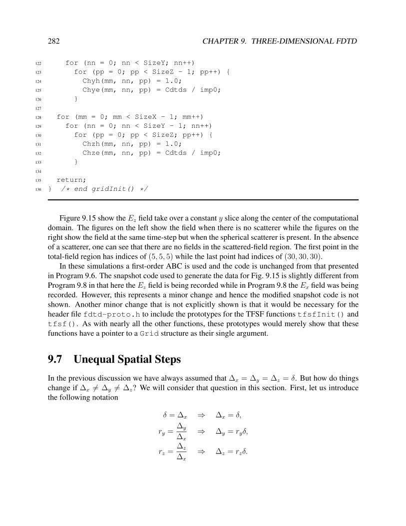
282 CHAPTER 9. THREE-DIMENSIONAL FDTD
122 for (nn = 0; nn < SizeY; nn++)123 for (pp = 0; pp < SizeZ - 1; pp++) 124 Chyh(mm, nn, pp) = 1.0;125 Chye(mm, nn, pp) = Cdtds / imp0;126 127
128 for (mm = 0; mm < SizeX - 1; mm++)129 for (nn = 0; nn < SizeY - 1; nn++)130 for (pp = 0; pp < SizeZ; pp++) 131 Chzh(mm, nn, pp) = 1.0;132 Chze(mm, nn, pp) = Cdtds / imp0;133 134
135 return;136 /* end gridInit() */
Figure 9.15 show the Ez field take over a constant y slice along the center of the computationaldomain. The figures on the left show the field when there is no scatterer while the figures on theright show the field at the same time-step but when the spherical scatterer is present. In the absenceof a scatterer, one can see that there are no fields in the scattered-field region. The first point in thetotal-field region has indices of (5, 5, 5) while the last point had indices of (30, 30, 30).
In these simulations a first-order ABC is used and the code is unchanged from that presentedin Program 9.6. The snapshot code used to generate the data for Fig. 9.15 is slightly different fromProgram 9.8 in that here the Ez field is being recorded while in Program 9.8 the Ex field was beingrecorded. However, this represents a minor change and hence the modified snapshot code is notshown. Another minor change that is not explicitly shown is that it would be necessary for theheader file fdtd-proto.h to include the prototypes for the TFSF functions tfsfInit() andtfsf(). As with nearly all the other functions, these prototypes would merely show that thesefunctions have a pointer to a Grid structure as their single argument.
9.7 Unequal Spatial StepsIn the previous discussion we have always assumed that ∆x = ∆y = ∆z = δ. But how do thingschange if ∆x 6= ∆y 6= ∆z? We will consider that question in this section. First, let us introducethe following notation
δ = ∆x ⇒ ∆x = δ,
ry =∆y
∆x
⇒ ∆y = ryδ,
rz =∆z
∆x
⇒ ∆z = rzδ.

9.7. UNEQUAL SPATIAL STEPS 283
10 20 30
5
10
15
20
25
30
(a) time−step 20, no scatterer
x location
z lo
ca
tio
n
10 20 30
5
10
15
20
25
30
(b) time−step 20, with sphere
x location
z lo
ca
tio
n
10 20 30
5
10
15
20
25
30
(c) time−step 40, no scatterer
x location
z lo
ca
tio
n
10 20 30
5
10
15
20
25
30
(d) time−step 40, with sphere
x location
z lo
ca
tio
n
10 20 30
5
10
15
20
25
30
(e) time−step 60, no scatterer
x location
z lo
ca
tio
n
10 20 30
5
10
15
20
25
30
(f) time−step 60, with sphere
x location
z lo
ca
tio
n
Figure 9.15: The Ez field over a constant-y plane taken from a 3D simulation in which the incidentelectric field is z-polarized and propagation is in the x direction. In the figures on the left noscatterer is present. Figures (a), (c), and (e) are taken at time-steps, 20, 40, and 60, respectively.The figures on the right show the field at the same time-steps, but a spherical scatterer is present.

284 CHAPTER 9. THREE-DIMENSIONAL FDTD
Furthermore, we will defined scaled field quantities such that
ex = ∆xEx, hx = ∆xHx,
ey = ∆yEy, hy = ∆yHy,
ez = ∆zEz, hz = ∆zHz.
With these definitions in place, let us consider a rewritten form of (9.18)
1
∆x
∆xEq+1x
[m+
1
2, n, p
]=
1− σ∆t
2ε
1 + σ∆t
2ε
1
∆x
∆xEqx
[m+
1
2, n, p
]+
1
1 + σ∆t
2ε
(∆t
ε∆y∆z
∆zH
q+ 12
z
[m+
1
2, n+
1
2, p
]−∆zH
q+ 12
z
[m+
1
2, n− 1
2, p
]− ∆t
ε∆y∆z
∆yH
q+ 12
y
[m+
1
2, n, p+
1
2
]−∆yH
q+ 12
y
[m+
1
2, n, p− 1
2
]). (9.39)
Multiplying through by ∆x and employing the definitions given above, this update equation be-comes
eq+1x
[m+
1
2, n, p
]=
1− σ∆t
2ε
1 + σ∆t
2ε
eqx
[m+
1
2, n, p
]+
1
1 + σ∆t
2ε
∆t
εδ
1
ryrz
(hq+ 1
2z
[m+
1
2, n+
1
2, p
]− hq+
12
z
[m+
1
2, n− 1
2, p
]−hq+ 1
2y
[m+
1
2, n, p+
1
2
]− hq+
12
y
[m+
1
2, n, p− 1
2
]). (9.40)
Importantly, all the (scaled) magnetic fields are multiplied by the same coefficient.From inspection of (9.18), it might have appeared that when the spatial step sizes are not equal,
another set of coefficients would have to be introduced (i.e., one for the term involving 1/∆y andone for the term involving 1/∆z). This is true if the field components are not scaled by theirrespective lengths. However, by scaling the fields, it is still only necessary to have two coefficientsper update equation.
The complete set up update equations for the scaled fields are:
hq+ 1
2x
[m,n+
1
2, p+
1
2
]=
1− σm∆t
2µ
1 + σm∆t
2µ
hq− 1
2x
[m,n+
1
2, p+
1
2
]+
1
1 + σm∆t
2µ
∆t
µδ
1
ryrz
(eqy
[m,n+
1
2, p+ 1
]− eqy
[m,n+
1
2, p
]−eqz
[m,n+ 1, p+
1
2
]− eqz
[m,n, p+
1
2
]), (9.41)

9.7. UNEQUAL SPATIAL STEPS 285
hq+ 1
2y
[m+
1
2, n, p+
1
2
]=
1− σm∆t
2µ
1 + σm∆t
2µ
hq− 1
2y
[m+
1
2, n, p+
1
2
]+
1
1 + σm∆t
2µ
∆t
µδ
ryrz
(eqz
[m+ 1, n, p+
1
2
]− eqz
[m,n, p+
1
2
]−eqx
[m+
1
2, n, p+ 1
]− eqx
[m+
1
2, n, p
]), (9.42)
hq+ 1
2z
[m+
1
2, n+
1
2, p
]=
1− σm∆t
2µ
1 + σm∆t
2µ
hq− 1
2z
[m+
1
2, n+
1
2, p
]+
1
1 + σm∆t
2ε
∆t
µδ
rzry
(eqx
[m+
1
2, n+ 1, p
]− eqx
[m+
1
2, n, p
]−eqy
[m+ 1, n+
1
2, p
]− eqy
[m,n+
1
2, p
]). (9.43)
eq+1x
[m+
1
2, n, p
]=
1− σ∆t
2ε
1 + σ∆t
2ε
eqx
[m+
1
2, n, p
]+
1
1 + σ∆t
2ε
∆t
εδ
1
ryrz
(hq+ 1
2z
[m+
1
2, n+
1
2, p
]− hq+
12
z
[m+
1
2, n− 1
2, p
]−hq+ 1
2y
[m+
1
2, n, p+
1
2
]− hq+
12
y
[m+
1
2, n, p− 1
2
]). (9.44)
eq+1y
[m,n+
1
2, p
]=
1− σ∆t
2ε
1 + σ∆t
2ε
eqy
[m,n+
1
2
]+
1
1 + σ∆t
2ε
∆t
εδ
ryrz
(hq+ 1
2x
[m,n+
1
2, p− 1
2
]− hq+
12
x
[m,n+
1
2, p− 1
2
]−hq+ 1
2z
[m+
1
2, n+
1
2, p
]− hq+
12
z
[m− 1
2, n+
1
2, p
]), (9.45)
eq+1z
[m,n, p+
1
2
]=
1− σ∆t
2ε
1 + σ∆t
2ε
eqz
[m,n, p+
1
2
]+
1
1 + σ∆t
2ε
∆t
εδ
rzry
(hq+ 1
2y
[m+
1
2, n, p+
1
2
]− hq+
12
y
[m− 1
2, n, p+
1
2
]−hq+ 1
2x
[m,n+
1
2, p+
1
2
]− hq+
12
x
[m,n− 1
2, p+
1
2
]). (9.46)
Thinking now in terms of coefficients, note that all the “self-term” coefficients are virtuallyunchanged from those given previously, i.e., Chxh , Chyh , Chzh , Cexe , Ceye , and Ceze are as given

286 CHAPTER 9. THREE-DIMENSIONAL FDTD
in (9.21), (9.23), (9.25), (9.27), (9.29), and (9.27), respectively. (There is a slight difference inthat those expressions listed the evaluation points merely in terms of a uniform spatial step size ofδ—one would now have to think in terms of ∆x, ∆y, and ∆z, for displacements in the x, y, and zdirections, respectively.)
The “cross” coefficients, such as Chze and Ceyh , are nearly the same as before where the onlydifferences are that δ specifically represents the spatial step ∆x, the scale factors ry and rz nowappear, and the locations are specifically in terms of ∆x, ∆y, and ∆z. These scaled coefficients arenow
Chxe(m,n+ 1/2, p+ 1/2) =1
1 + σm∆t
2µ
∆t
µδ
1
ryrz
∣∣∣∣∣m∆x,(n+1/2)∆y ,(p+1/2)∆z
, (9.47)
Chye(m+ 1/2, n, p+ 1/2) =1
1 + σm∆t
2µ
∆t
µδ
ryrz
∣∣∣∣∣(m+1/2)∆x,n∆y ,(p+1/2)∆z
, (9.48)
Chze(m+ 1/2, n+ 1/2, p) =1
1 + σm∆t
2µ
∆t
µδ
rzry
∣∣∣∣∣(m+1/2)∆x,(n+1/2)∆y ,p∆z
, (9.49)
Cexh(m+ 1/2, n, p) =1
1 + σ∆t
2ε
∆t
εδ
1
ryrz
∣∣∣∣∣(m+1/2)∆x,n∆y ,p∆z
, (9.50)
Ceyh(m,n+ 1/2, p) =1
1 + σ∆t
2ε
∆t
εδ
ryrz
∣∣∣∣∣m∆x,(n+1/2)∆y ,p∆z
, (9.51)
Cezh(m,n, p+ 1/2) =1
1 + σ∆t
2ε
∆t
εδ
rzry
∣∣∣∣∣m∆x,n∆y ,(p+1/2)∆z
. (9.52)
Finally, stability dictates that
∆t ≤1
c√
1∆2x
+ 1∆2y
+ 1∆2z
(9.53)
which, after employing the definitions given above and rearranging, can be written as
c∆t
δ≤ 1√
1 + 1r2y
+ 1r2z
(9.54)
Note that when ry = rz = 1 all the update equations and coefficients are identical to what waspreviously given for a uniform grid. This may seem rather odd because now we are discussingscaled fields instead of the fields themselves, e.g., we are dealing with ex = ∆xEx instead of Ex.(The scaled “electric” and “magnetic” fields have units of volts and amperes, respectively, insteadof volts per meter and ampere per meter, and hence these fields are really voltages and currents.)However, one must keep in mind that for these scaled fields the source terms would correspondinghave to be scaled. For example, if there were an additive source current in the update equation forEx, in the scaled version of the update equation this source term would also be scaled by ∆x. Thus,

9.7. UNEQUAL SPATIAL STEPS 287
if one were to compare the values in a simulation involving the scaled and unscaled x-componentof the electric field, the scaled values would be larger by a factor of ∆x. When the scaled field isdivided by ∆x one obtains the same electric field that would be obtained directly from a simulationwith unscaled fields.
Returning to the question raised at the beginning of the section: But how do things change if∆x 6= ∆y 6= ∆z? The answer is that very little changes. The same code can be used for simulationswith either equal or unequal spatial steps. The only differences will be in the Courant number, asgiven by (9.54), in the coefficients of the “cross” coefficients, as given by (9.47)–(9.52), and thefact that one is now modeling the scaled fields rather than the fields themselves. Source termsshould also be appropriately scaled but that will not be considered further here.

288 CHAPTER 9. THREE-DIMENSIONAL FDTD

Chapter 10
Dispersive Material
10.1 IntroductionFor many problems one can obtain acceptably accurate results by assuming material parameters areconstants. However, constant material parameters are inherently an approximation. For example,it is impossible to have a lossless dielectric with constant permittivity (except, of course, for freespace). If such a material did exist it would violate causality. (For a material to behave causally, theKramers-Kronig relations show that for any deviation from free-space behavior the imaginary partof the permittivity or permeability, i.e., the loss, cannot vanish for all frequencies. Nevertheless, asfar as causality is concerned, the loss can be arbitrarily small.)
A non-unity, scalar, constant relative permittivity is equivalent to assuming the polarizationof charge within a material is instantaneous and in perfect proportion to the applied electric field.Furthermore, the reaction is the same at all frequencies, is the same in all directions, is the same forall times, and the same proportionality constant holds for all field strengths. In reality, essentiallynone of the these assumptions are absolutely correct. The relationship between the electric fluxdensity D and the electric field E can reflect all the complexity of the real world. Instead of simplyhaving D = εE where ε is a scalar constant, one can make ε a tensor to describe different behaviorsin different directions (off diagonal terms would indicate the amount of coupling from one directionto another). The permittivity can also be written as a nonlinear function of the applied electric fieldto account for nonlinear media. The material parameters can be functions of time (such as mightpertain to a material which is being heated). Finally, one should not forget that the permittivity canbe a function of position to account for spatial inhomogeneities.
When the speed of light in a material is a function of frequency, the material is said to bedispersive. The fact that the FDTD grid is dispersive has been discussed in Chap. 7. That dispersionis a numerical artifact and is distinct from the subject of this chapter. We have also consideredlossy materials. Even when the conductivity of a material is assumed to be constant, the materialis dispersive (ref. (5.69) which shows that the phase constant is not linearly proportional to thefrequency which must be the case for non-dispersive propagation).
When the permittivity or permeability of a material are functions of frequency, the material isdispersive. In time-harmonic form one can account for the frequency dependence of permittivityby writing D(ω) = ε(ω)E(ω), where a caret is used to indicate a quantity in the frequency domain.
†Lecture notes by John Schneider. fdtd-dispersive-material.tex
289

290 CHAPTER 10. DISPERSIVE MATERIAL
This expression is simple in the frequency domain, but the FDTD method is a time-domain tech-nique. The multiplication of harmonic functions is equivalent to convolution in the time domain.Therefore it requires some additional effort to model these types of dispersive materials. We startwith a brief review of dispersive materials and then consider two ways in which to model suchmaterials in the FDTD method.
10.2 Constitutive Relations and Dispersive MediaThe electric flux density and magnetic field are related to the electric field and the magnetic fluxdensity via
D = ε0E + P, (10.1)
H =B
µ0
−M, (10.2)
where P and M account for the electric and magnetic dipoles, respectively, induced in the media.Keep in mind that force on a charge is a function of E and B so in some sense E and B are the“real” fields. The polarization vector P accounts for the local displacement of bound charge in amaterial. Because of the way in which P is constructed, by adding it to ε0E the resulting electricflux density D has the local effect of bound charge removed. In this way, the integral of D overa closed surface yields the free charge (thus Gauss’s law, as expressed using the D field, is truewhether material is present or not).
The magnetic field H ignores the local effect of bound charge in motion. Thus, the integrationof H over a closed loop yields the current flowing through the surface enclosed by that loop wherethe current is due to either the flow of free charge or displacement current (i.e., the integral formof Ampere’s law). Rearranging the terms in (10.2) and multiplying by µ0 yields an expression forthe magnetic flux density∗, i.e.,
B = µ0(H + M). (10.3)
At a given frequency, for a linear, isotropic medium, the polarization vectors can be related tothe electric and magnetic fields via an electric or magnetic susceptibility
P(ω) = ε0χe(ω)E(ω), (10.4)M(ω) = χm(ω)H(ω), (10.5)
where χe(ω) and χm(ω) are the electric and magnetic susceptibility, respectively.† Thus we canwrite
D(ω) = ε0E(ω) + ε0χe(ω)E(ω), (10.6)B(ω) = µ0H(ω) + µ0χm(ω)H(ω). (10.7)
∗Note that there are those (e.g., Feynman) who advocate that one should avoid using D and H. Others (e.g.,Sommerfeld) have discussed the unfortunate naming of the magnetic field and the magnetic flux density. However,those issues are peripheral to the main subject of interest here and we will employ the notation and usage as iscommonly found in engineering electromagnetics.†Here we will assume that χe(ω) and χm(ω) are not functions of time. Thus frequency response of the material
“today” is the same as it will be “tomorrow.”

10.2. CONSTITUTIVE RELATIONS AND DISPERSIVE MEDIA 291
For the time being we restrict discussion to the electric fields where the permittivity ε(ω) is definedas
ε(ω) = ε0εr(ω) = ε0(ε∞ + χe(ω)). (10.8)
where εr is the relative permittivity and, as will be seen, the constant ε∞ accounts for the effect ofthe charged material at high frequencies where the susceptibility function goes to zero.
The time-domain electric flux density can be obtain by inverse transforming (10.6). The prod-uct of χe and E in the frequency domain yields a convolution in the time domain. The fields areassumed to be zero prior to t = 0, so this yields
D(t) = ε0E(t) +
t∫τ=0
χe(τ)E(t− τ)dτ (10.9)
where χe(t) is the inverse transform of χe(ω):
χe(t) =1
2π
∞∫−∞
χe(ω)ejωtdω. (10.10)
The time-domain function ε0χe(t) corresponds to the polarization vector P(t) for an impulsiveelectric field—effectively the impulse response of the medium.
We now consider three common susceptibility functions. As will be shown these are based oneither simple mechanical or electrical models.
10.2.1 Drude MaterialsIn the Drude model, which often provides a good model of the behavior of conductors, charges areassumed to move under the influence of the electric field but they experience a damping force aswell. This can be described by the following simple mechanical model
Md2x
dt2= QE(t)−Mg
dx
dt(10.11)
where M is the mass of the charge, g is the damping coefficient, Q is the amount of charge, and xis the displacement of the charge (the displacement is assumed to be in an arbitrary direction andnot restricted to the x axis despite the use of the symbol x). The left side of this equation is masstimes acceleration and the right side is the sum of the forces on the charge, i.e., a driving force anda damping force. Rearranging this and converting to the frequency domain yields
M(jω)2x(ω) +Mg(jω)x(ω) = QE(ω). (10.12)
Thus the displacement can be expressed as
x(ω) = − Q
M (ω2 − jgω)E(ω). (10.13)
The polarization vector P is related to the dipole moment of individual charges. IfN is the numberof dipoles per unit volume, the polarization vector is given by
P = NQx. (10.14)

292 CHAPTER 10. DISPERSIVE MATERIAL
Note that P has units of charge per units area (C/m2) and thus, as would be expected from (10.1),has the same units as electric flux. Combining (10.13) and (10.14) yields
P(ω) = −ε0NQ2
Mε0
ω2 − jgωE(ω). (10.15)
The electric susceptibility for Drude materials is thus given by
χe(ω) = −ω2p
ω2 − jgω(10.16)
where ω2p = NQ2/(Mε0). However, we are not overly concerned with the specifics behind any
one constant. For example, some authors may elect to combine the mass and damping coefficientwhich were kept as separate quantities in (10.11) (the product of the two dictates the dampingforce). Regardless of how the constants are defined, ultimately the Drude susceptibility will takethe form shown in (10.16).
The relative permittivity for a Drude material can thus be written
εr(ω) = ε∞ −ω2p
ω2 − jgω. (10.17)
Note that as ω goes to infinity the relative permittivity reduces to ε∞. Consider a rather specialcase in which ε∞ = 1 and g = 0. When ω = ωp/
√2 the relative permittivity is −1. It is
possible, at least to some extent, to construct a material which has not only this kind of behaviorfor permittivity but also for the behavior for the permeability, i.e., µr = εr = −1. This kindof material, which is known by various names including meta material, double-negative material,backward-wave material, and left-handed material, possesses many interesting properties. Someproperties of these “meta materials” are also rather controversial as some people have made claimsthat others dispute (such as the ability to construct a “perfect” lens using a planar slab of thismaterial).
The impulse response for the medium is the inverse Fourier transform of (10.16):
χe(t) =ω2p
g
(1− e−gt
)u(t) (10.18)
where u(t) is the unit step function. The factor g is seen to determine the rate at which the responsegoes to zero, i.e., its inverse is the relaxation time. The factor ωp is known as the plasma frequency.
10.2.2 Lorentz MaterialLorentz material is based on a second-order mechanical model of charge motion. In this case, inaddition to a damping force, there is a restoring force (effectively a spring force which wants tobring the charge back to its initial position). The sum of the forces can be expressed as
Md2x
dt2= QE(t)−Mg
dx
dt−MKx. (10.19)

10.2. CONSTITUTIVE RELATIONS AND DISPERSIVE MEDIA 293
The terms in commons with those in (10.11) as they had in the case of the Drude model. Theadditional term represents the restoring force (which is proportional to the displacement) and isscaled by the spring constant K.
Converting to the frequency domain and rearranging yields
−Mω2x(ω) + jMgωx(ω) +MKx(ω) = QE(ω). (10.20)
Thus the displacement is given by
x(ω) =Q
M (K + jgω − ω2)E(ω). (10.21)
Relating displacement to the polarization vector via P = NQx yields
P(ω) = ε0NQ2
Mε0 (K + jgω − ω2)E(ω). (10.22)
From this the susceptibility is identified as
χe(ω) =NQ2
Mε0 (K + jgω − ω2)(10.23)
However, as before, the important thing is the form of the function, not the individual constants.We thus write this as
χe(ω) =ε`ω
2`
ω2` + 2jg`ω − ω2
(10.24)
where ω` is the undamped resonant frequency, g` is the damping coefficient, and ε` (together withε∞) accounts for the relatively permittivity at zero frequency. The corresponding relative permit-tivity is given by
εr(ω) = ε∞ +ε`ω
2`
ω2` + 2jg`ω − ω2
. (10.25)
Note that when the frequency goes to zero the relative permittivity becomes ε∞+ ε` whereas whenthe frequency goes to infinity the relative permittivity is simply ε∞.
The time-domain form of the susceptibility function is given by the inverse transform of (10.24).This yields
χe(t) =ε`ω
2`√
ω2` − g2
`
e−g`t sin
(t√ω2` − g2
`
)u(t). (10.26)
10.2.3 Debye MaterialDebye materials can be thought of as a simple RC circuit where the amount of polarization is re-lated to the voltage across the capacitor. The “source” driving the circuit is the electric field. For astep in the source, there may be a constant polarization. As the frequency goes to infinity, the po-larization goes to zero (leaving just the constant residual high-frequency term). The susceptibilityis thus written
χe(ω) =εd
1 + jωτd(10.27)

294 CHAPTER 10. DISPERSIVE MATERIAL
where τd is the time constant and εd (together with ε∞) accounts for the relative permittivity whenthe frequency is zero. The relative permittivity is given by
εr(ω) = ε∞ +εd
1 + jωτd. (10.28)
The time-domain form of the susceptibility function is
χe(t) =εdτde−t/τdu(t). (10.29)
10.3 Debye Materials Using the ADE MethodThe finite-difference approximation of the differential equation that relates the polarization and theelectric field can be used to obtain the polarization at future times in terms of its past value andan expression involving the electric field. By doing so, one can obtain a consistent FDTD modelthat requires that a quantity related to the polarization be stored as an additional variable. Thisapproach is known as the auxiliary differential equation (ADE) method.
In the frequency domain Ampere’s law can be written
ε0ε∞jωE + σE + Jp = ∇× H (10.30)
where the polarization current Jp is given by
Jp = jωP = jωε0χeE. (10.31)
For a Debye material this becomes
Jp = jωε0εd
1 + jωτE. (10.32)
Multiplying through by 1 + jωτ yields
Jp + jωτ Jp = jωε0εdE. (10.33)
Converting to the time domain produces
Jp + τ∂Jp∂t
= ε0εd∂E
∂t. (10.34)
Discretizing this about the time-step q + 1/2 yields
Jq+1p + Jqp
2+ τ
Jq+1p − Jqp
∆t
= ε0εdEq+1 − Eq
∆t
. (10.35)
Since we are assuming an isotropic medium, the polarization current is aligned with the electricfield. Hence in (10.35) the x component of Jp depends only on the x component of E (and similarlyfor the y and z components).

10.3. DEBYE MATERIALS USING THE ADE METHOD 295
Solving (10.35) for Jq+1p yields
Jq+1p =
1− ∆t
2τ
1 + ∆t
2τ
Jqp +∆t
τ
1 + ∆t
2τ
ε0εd∆t
(Eq+1 − Eq
). (10.36)
Whatever the time-constant τ is, it can be expressed in terms of some multiple of the time-step,i.e., τ = Nτ∆t where Nτ does not need to be an integer. As will be shown, it is convenient tomultiply both sides of (10.36) by the spatial step size. We will assume a uniform grid in which∆x = ∆y = ∆z = δ. Thus (10.36) can be written
δJq+1p =
1− 12Nτ
1 + 12Nτ
δJqp +1Nτ
1 + 12Nτ
ε0εdδ
∆t
(Eq+1 − Eq
). (10.37)
Consider the factor ε0εdδ/∆t:
ε0εdδ
∆t
=
√ε0µ0εdδ√µ0
ε0∆t
=εdδ
η0c∆t
=εdη0Sc
. (10.38)
Therefore (10.37) can be written
δJq+1p = Cjj δJ
qp + Cje
(Eq+1 − Eq
), (10.39)
where
Cjj =1− 1
2Nτ
1 + 12Nτ
, (10.40)
Cje =1Nτ
1 + 12Nτ
εdη0Sc
. (10.41)
Recall that Ampere’s law is discretized about the time-step (q + 1/2)∆t. Since the polarizationcurrent appears in Ampere’s law, we thus need an expression for δJq+1/2
p . This is simply given bythe average of δJq+1
p (which is given by (10.39)) and δJqp:
δJq+1/2p =
δJq+1p + δJqp
2=
1
2
([1 + Cjj ]δJ
qp + Cje
(Eq+1 − Eq
)). (10.42)
The discrete time-domain form of Ampere’s law expanded about the time-step (q + 1/2) is
ε0ε∞Eq+1 − Eq
∆t
+ σEq+1 + Eq
2+ Jq+1/2
p = ∇×Hq+1/2. (10.43)
Multiplying through by δ and using (10.42) in (10.43) yields
ε∞ε0δ
∆t
(Eq+1 − Eq
)+σδ
2
(Eq+1 + Eq
)+
1
2
([1 + Cjj ]δJ
qp + Cje
(Eq+1 − Eq
))= δ∇×Hq+1/2.
(10.44)

296 CHAPTER 10. DISPERSIVE MATERIAL
The curl of the magnetic field, which involves spatial derivatives, will have a δ in the denominatorof the finite differences. Thus δ∇ × Hq+1/2 will involve merely the difference of the variousmagnetic-field components.
Regrouping terms in (10.44) produces
Eq+1
(ε∞ε0δ
∆t
+σδ
2+
1
2Cje
)= Eq
(ε∞ε0δ
∆t
− σδ
2+
1
2Cje
)+ δ∇×Hq+1/2 − 1
2[1 + Cjj ] δJ
qp.
(10.45)The term multiplying the electric fields can be written as
ε∞ε0δ
∆t
(1± σ∆t
2ε∞ε0+
Cje∆t
2ε∞ε0δ
)=
ε∞η0Sc
(1± σ∆t
2ε∞ε0+Cjeη0Sc
2ε∞
). (10.46)
Therefore (10.45) can be written
Eq+1 =1− σ∆t
2ε∞ε0+
Cjeη0Sc2ε∞
1 + σ∆t
2ε∞ε0+
Cjeη0Sc2ε∞
Eq +
η0Scε∞
1 + σ∆t
2ε∞ε0+
Cjeη0Sc2ε∞
(δ∇×Hq+1/2 − 1
2[1 + Cjj ] δJ
qp
).
(10.47)The way in which the term σ∆t/(2ε0) could be expressed in terms of the skin depth was discussedin Sec. 5.7.
The FDTD model of a Debye material would be implemented as follows:
1. Update the magnetic fields in the usual way. Hq−1/2 ⇒ Hq+1/2.
2. For each electric-field component, do the following:
(a) Copy the electric field to a temporary variable. Etmp = Eq.
(b) Update the electric field using (10.47). Eq ⇒ Eq+1.
(c) Update the polarization current (actually δ times the polarization current) using (10.39).Jqp ⇒ Jq+1
p . This update requires both Eq+1 and Eq (which is stored in Etmp).
3. Repeat.
The polarization current (actually the product of the spatial step-size and the polarization current,i.e., δJp) must be stored as a separate quantity. Of course it only needs to be stored for nodes atwhich it is non-zero.
If the polarization current is initially zero and Cje is zero, the polarization current will alwaysbe zero and the material behaves as a standard non-dispersive material (although, of course, dis-persion is always present in the grid itself). Thus the update equations presented here can be usedthroughout a simulation which is a mix of dispersive and non-dispersive media. One merely has toset the constants to the appropriate values for a given location.
10.4 Drude Materials Using the ADE MethodThe electric susceptibility for a Drude material is given in (10.16) and can also be written
χe(ω) =ω2p
jω(jω + g). (10.48)

10.4. DRUDE MATERIALS USING THE ADE METHOD 297
The associated polarization current is
Jp = jωP = jωε0χeE = jωε0ω2p
jω(jω + g)E. (10.49)
Canceling jω and cross multiplying by g + jω yields
gJp + jωJp = ε0ω2pE. (10.50)
Expressed in the time-domain, this is
gJp +∂Jp∂t
= ε0ω2pE. (10.51)
Discretizing time and expanding this about the time-step q + 1/2 yields
gJq+1p + Jqp
2+
Jq+1p − Jqp
∆t
= ε0ω2p
Eq+1 + Eq
2. (10.52)
Solving for Jq+1p we obtain
Jq+1p =
1− g∆t
2
1 + g∆t
2
Jqp +1
1 + g∆t
2
ε0ω2p∆t
2
(Eq+1 + Eq
). (10.53)
The damping or loss term g is the inverse of the relaxation time and hence can be expressed as amultiple of the number of time steps, i.e.,
g =1
Ng∆t
(10.54)
where Ng does not need to be integer. Consider the term multiplying the electric field
ε0ω2p∆t
2=
√ε0µ04π2f 2
p∆t√µ0
ε02
=2π2c2∆t
η0λ2pc
=2π2c∆t
η0(Npδ)2=
2π2Scη0N2
p δ(10.55)
where fp is the plasma frequency in Hertz, λp is the free-space wavelength at this frequency, andNp is the number of points per wavelength at the plasma frequency. Since this term contains δ inthe denominator, we multiply (10.53) by δ to obtain
δJq+1p = Cjj δJ
qp + Cje
(Eq+1 + Eq
)(10.56)
where
Cjj =1− 1
2Ng
1 + 12Ng
, (10.57)
Cje =1
1 + 12Ng
2π2Scη0N2
p
. (10.58)

298 CHAPTER 10. DISPERSIVE MATERIAL
Note the similarity between (10.39) and (10.56). These equations have nearly identical forms butthe constants are different and there is a different sign associated with the “old” value of the electricfield.
The general discretized form of Ampere’s law expanded about the time-step (q + 1/2) is un-changed from (10.43) and is repeat below
ε0ε∞Eq+1 − Eq
∆t
+ σEq+1 + Eq
2+ Jq+1/2
p = ∇×Hq+1/2. (10.59)
As before, δJq+1/2p can be obtained by the average of δJq+1
p and δJqp:
δJq+1/2p =
δJq+1p + δJqp
2=
1
2
([1 + Cjj ]δJ
qp + Cje
(Eq+1 + Eq
)). (10.60)
Multiplying through by δ and using (10.60) for the polarization current yields
ε∞ε0δ
∆t
(Eq+1 − Eq
)+σδ
2
(Eq+1 + Eq
)+
1
2
([1 + Cjj ]δJ
qp + Cje
(Eq+1 + Eq
))= δ∇×Hq+1/2.
(10.61)Note that, other than the constants being those for a Drude material, the only way in which thisexpression differs from (10.44) is the sign of the “old” electric field associated with the polarizationcurrent. Therefore (10.47) again yields the expression for the “future” electric field if we make theappropriate change of sign. The result is
Eq+1 =1− σ∆t
2ε∞ε0− Cjeη0Sc
2ε∞
1 + σ∆t
2ε∞ε0+
Cjeη0Sc2ε∞
Eq +
η0Scε∞
1 + σ∆t
2ε∞ε0+
Cjeη0Sc2ε∞
(δ∇×Hq+1/2 − 1
2[1 + Cjj ] δJ
qp
).
(10.62)The implementation of an FDTD algorithm for Drude material now parallels that for Debye
material:
1. Update the magnetic fields in the usual way. Hq−1/2 ⇒ Hq+1/2.
2. For each electric-field component, do the following
(a) Copy the electric field to a temporary variable. Etmp = Eq.
(b) Update the electric field using (10.62). Eq ⇒ Eq+1.
(c) Update the polarization current (actually δ times the polarization current) using (10.56).Jq ⇒ Jq+1. This update requires both Eq+1 and Eq (which is stored in Etmp).
3. Repeat.
10.5 Magnetically Dispersive MaterialIn the frequency domain Faraday’s law is
∇× E = −jωB− σmH (10.63)

10.5. MAGNETICALLY DISPERSIVE MATERIAL 299
where σm is the magnetic conductivity. Generalizing (10.7) slightly, the permeability can be writ-ten as
µ(ω) = µ0µr(ω) = µ0(µ∞ + χm(ω)). (10.64)
where the factor µ∞ accounts for the permeability at high frequencies. Faraday’s law can thus bewritten
∇× E = −jωµ0µ∞H(ω)− σmH− Jm. (10.65)
where the magnetic polarization current Jm is given by
Jm = jωµ0M = jωµ0χm(ω)H(ω). (10.66)
The derivation of the equations which govern an FDTD implementation of a magneticallydispersive material parallel that of electrically dispersive material. Here we consider the case ofDrude dispersion where
χm(ω) = −ω2p
ω2 − jgω=
ω2p
jω(jω + g). (10.67)
(The plasma frequency ωp and damping term g for magnetic susceptibility are distinct from thoseof electric susceptibility.) Thus the polarization current and magnetic field are related by
Jm = jωµ0
ω2p
jω(jω + g)H =
µ0ω2p
(jω + g)H. (10.68)
Multiplying by g + jω yields(g + jω)Jm = µ0ω
2pH. (10.69)
The time-domain equivalent of this is
gJm +∂Jm∂t
= µ0ω2pH. (10.70)
Discretizing time and expanding this about the time-step q yields
gJq+1/2m + J
q−1/2m
2+
Jq+1/2m − J
q−1/2m
∆t
= µ0ω2p
Hq+1/2 + Hq−1/2
2. (10.71)
Solving for Jq+1/2m yields
Jq+1/2m =
1− g∆t
2
1 + g∆t
2
Jq−1/2m +
1
1 + g∆t
2
µ0ω2p∆t
2
(Hq+1/2 + Hq−1/2
). (10.72)
Consider the term multiplying the magnetic field
µ0ω2p∆t
2=
õ0
ε0
√ε0µ04π2f 2
p∆t
2=
2π2η0c2∆t
λ2pc
=2π2η0c∆t
(Npδ)2=
2π2η0ScN2p δ
. (10.73)
where, as before, fp is the plasma frequency in Hertz, λp is the free-space wavelength at this fre-quency, and Np is the number of points per wavelength at the plasma frequency. Again expressing

300 CHAPTER 10. DISPERSIVE MATERIAL
the damping coefficient in terms of some multiple of the time step, i.e., g = 1/(Ng∆t), multiply-ing all terms in (10.72) by δ, and employing the final form of the term given in (10.73), the updateequation for the polarization current can be written as
δJq+1/2m = Cjj δJ
q−1/2m + Cjh
(Hq+1/2 + Hq−1/2
)(10.74)
where
Cjj =1− 1
2Ng
1 + 12Ng
, (10.75)
Cjh =1
1 + 12Ng
2π2η0ScN2p
. (10.76)
To obtain the magnetic polarization current at time-step q, the current at time-steps q + 1/2 andq − 1/2 are averaged:
δJqm =δJ
q+1/2m + δJ
q−1/2m
2=
1
2
([1 + Cjj ]δJ
q−1/2m + Cjh
(Hq+1/2 + Hq−1/2
)). (10.77)
The discretized form of Faraday’s law expanded about time-step q is
−µ0µ∞Hq+1/2 −Hq−1/2
∆t
− σmHq+1/2 −Hq−1/2
2− Jqm = ∇× Eq. (10.78)
Multiplying through by −δ and using (10.77) for the polarization current yields
µ∞µ0δ
∆t
(Hq+1/2 −Hq−1/2
)+σmδ
2
(Hq+1/2 + Hq−1/2
)+
1
2
([1 + Cjj ]δJ
q−1/2m + Cjh
(Hq+1/2 + Hq−1/2
))= −δ∇× Eq. (10.79)
After regrouping terms we obtain
Hq+1/2
(µ∞µ0δ
∆t
+σmδ
2+
1
2Cjh
)=
Hq−1/2
(µ∞µ0δ
∆t
− σmδ
2+
1
2Cjh
)− δ∇× Eq − 1
2[1 + Cjj ] δJ
q−1/2m . (10.80)
The factor µ0δ/∆t is equivalent to η0/Sc so that the update equation for the magnetic field can bewritten
Hq+1/2 =1− σm∆t
2µ∞µ0− CjhSc
2η0µ∞
1 + σm∆t
2µ∞µ0+
CjhSc2η0µ∞
Hq−1/2 +
Scη0µ∞
1 + σm∆t
2µ∞µ0+
CjhSc2η0µ∞
(−δ∇× Eq − 1
2[1 + Cjj ] δJ
q−1/2m
).
(10.81)An FDTD model of a magnetically dispersive material would be implemented as follows:
1. For each magnetic-field component, do the following

10.6. PIECEWISE LINEAR RECURSIVE CONVOLUTION 301
(a) Copy the magnetic field to a temporary variable. Htmp = Hq−1/2.
(b) Update the magnetic field using (10.81). Hq−1/2 ⇒ Hq+1/2.
(c) Update the polarization current (actually δ times the polarization current) using (10.74).Jq−1/2m ⇒ J
q+1/2m . This update requires both Hq+1/2 and Hq−1/2 (which is stored in
Htmp).
2. Update the electric fields in whatever way is appropriate (which may include the dispersiveimplementations described previously) Eq ⇒ Eq+1.
3. Repeat.
10.6 Piecewise Linear Recursive ConvolutionAn alternative implementation of dispersive material is offered by the piecewise linear recursiveconvolution (PLRC) method. Recall that multiplication in the frequency domain is equivalent toconvolution in the time domain. Thus, the frequency-domain relationship
D(ω) = ε0ε∞E(ω) + ε0χe(ω)E(ω) (10.82)
is equivalent to the time-domain relationship
D(t) = ε0ε∞E(t) + ε0
t∫ζ=0
E(t− ζ)χe(ζ)dζ (10.83)
where ζ is a dummy variable of integration. In discrete form the electric flux density at time-stepq∆t can be written
Dq = ε0ε∞Eq + ε0
q∆t∫ζ=0
E(q∆t − ζ)χe(ζ)dζ. (10.84)
Although in an FDTD simulation the electric field E would only be available at discrete pointsin time, we wish to treat the field as if it varies continuously insofar as the integral is concerned.This is accomplished by assuming the field varies linearly between sample points. For example,assume the continuous variable t is between i∆t and (i+ 1)∆t. Over this range the electric field isapproximated by
E(t) = Ei +Ei+1 − Ei
∆t
(t− i∆t) for i∆t ≤ t ≤ (i+ 1)∆t. (10.85)
When t is equal to i∆t we obtain Ei and when t is (i + 1)∆t we obtain Ei+1. The field varieslinearly between these points.
To obtain a more general representation of the electric field, let us define the pulse functionpi(t) which is given by
pi(t) =
1 if i∆t ≤ t < (i+ 1)∆t,0 otherwise. (10.86)

302 CHAPTER 10. DISPERSIVE MATERIAL
Using this pulse function the electric field can be written as
E(t) =M−1∑i=0
[Ei +
Ei+1 − Ei
∆t
(t− i∆t)
]pi(t). (10.87)
This provides a piecewise-linear approximation of the electric field over M segments. Despite thesummation, the pulse function ensures that only one segment is turned on for any given value of t.Hence the summation can be thought of as serving more to collect together the various segmentsrather than as serving to add several terms.
In the integrand of (10.84) the argument of the electric field is q∆t − ζ where q∆t is constantwith respect to the variable of integration ζ . When ζ varies from i∆t to (i+ 1)∆t the electric fieldshould vary from the discrete points Eq−i to Eq−i−1. Thus, the electric field can be represented by
E(q∆t − ζ) = Eq−i +Eq−i−1 − Eq−i
∆t
(ζ − i∆t) for i∆t ≤ ζ ≤ (i+ 1)∆t. (10.88)
Using the pulse function, the field over all values of ζ can be written
E(q∆t − ζ) =
q−1∑i=0
[Eq−i +
Eq−i−1 − Eq−i
∆t
(ζ − i∆t)
]pi(ζ). (10.89)
Note the limits of the summation. The upper limit of integration is q∆t which corresponds to theend-point of the segment which varies from (q − 1)∆t to q∆t. This segment has an index of q − 1(segment 0 varies from 0 to ∆t, segment 1 varies from ∆t to 2∆t, and so on). The lower limit usedhere is not actually dictated by the electric field. Rather, when we combine the electric field withthe susceptibility function the product is zero for ζ less than zero since the susceptibility is zerofor ζ less than zero (due to the material impulse response being causal). Hence we start the lowerlimit of the summation at zero.
Substituting (10.89) into (10.84) yields
Dq = ε0ε∞Eq + ε0
q∆t∫ζ=0
q−1∑i=0
[Eq−i +
Eq−i−1 − Eq−i
∆t
(ζ − i∆t)
]pi(ζ)χe(ζ)dζ. (10.90)
The summation and integration can be interchanged. However, the pulse function dictates that theintegration only needs to be carried out over the range of values where the pulse function is unity.Thus we can write
Dq = ε0ε∞Eq + ε0
q−1∑i=0
(i+1)∆t∫ζ=i∆t
[Eq−i +
Eq−i−1 − Eq−i
∆t
(ζ − i∆t)
]χe(ζ)dζ. (10.91)
The samples of the electric field are constants with respect to the variable of integration and can betaken outside of the integral. This yields
Dq = ε0ε∞Eq +
ε0
q−1∑i=0
Eq−i
(i+1)∆t∫ζ=i∆t
χe(ζ)dζ
+Eq−i−1 − Eq−i
∆t
(i+1)∆t∫ζ=i∆t
(ζ − i∆t)χe(ζ)dζ
.(10.92)

10.6. PIECEWISE LINEAR RECURSIVE CONVOLUTION 303
To simplify the notation, we define the following
χi =
(i+1)∆t∫ζ=i∆t
χe(ζ)dζ, (10.93)
ξi =1
∆t
(i+1)∆t∫ζ=i∆t
(ζ − i∆t)χe(ζ)dζ. (10.94)
This allows us to write
Dq = ε0ε∞Eq + ε0
q−1∑i=0
[Eq−iχi +
(Eq−i−1 − Eq−i) ξi] . (10.95)
In discrete form and using the electric flux density, Ampere’s law can be written
∇×Hq+1/2 =Dq+1 −Dq
∆t
. (10.96)
Equation (10.95) gives Dq in terms of the electric field. This equation can also be used to expressDq+1 in terms of the electric field: one merely replaces q with q + 1. This yields
Dq+1 = ε0ε∞Eq+1 + ε0
q∑i=0
[Eq−i+1χi +
(Eq−i − Eq−i+1
)ξi]. (10.97)
In order to obtain an update equation for the electric field, we must express Eq+1 in terms of otherknown (or past) quantities. As things stand now, there is an Eq+1 “buried” inside the the summationin (10.97). To express that explicitly, we extract the i = 0 term and then have the summation startfrom i = 1. This yields
Dq+1 = ε0ε∞Eq+1 + ε0Eq+1χ0 + ε0
(Eq − Eq+1
)ξ0
+ε0
q∑i=1
[Eq−i+1χi +
(Eq−i − Eq−i+1
)ξi]. (10.98)
Ultimately we want to combine the summations in (10.95) and (10.98) and thus the limits of thesummations must be the same. The limits of the summation in (10.98) can be adjusting by using anew index i′ = i− 1 (thus i = i′ + 1). Substituting i′ for i, (10.98) can be written
Dq+1 = Eq+1ε0(ε∞ + χ0 − ξ0) + Eqε0ξ0
+ε0
q−1∑i′=0
[Eq−i′χi
′+1 +(Eq−i′−1 − Eq−i′
)ξi′+1]. (10.99)
Since i′ is just an index, we can return to calling is merely i.

304 CHAPTER 10. DISPERSIVE MATERIAL
The temporal finite-difference of the flux density is obtained by combining (10.95) and (10.99).The result is
Dq+1 −Dq
∆t
=1
∆t
(Eq+1ε0(ε∞ − χ0 + ξ0) + Eqε0(−ε∞ + ξ0)
−ε0q−1∑i=0
[Eq−i∆χi +
(Eq−i−1 − Eq−i)∆ξi
])(10.100)
where
∆χi = χi − χi+1, (10.101)∆ξi = ξi − ξi+1. (10.102)
The summation in (10.100) does not contain Eq+1. Hence, using (10.100) to replace the rightside of (10.96) and solving for Eq+1 yields
Eq+1 =ε∞ − ξ0
ε∞ + χ0 − ξ0Eq +
∆t
ε0
ε∞ + χ0 − ξ0∇×Hq+1/2 +
1
ε∞ + χ0 − ξ0Ψq (10.103)
where Ψq, known as the recursive accumulator, is given by
Ψq =
q−1∑i=0
[Eq−i∆χi +
(Eq−i−1 − Eq−i)∆ξi
](10.104)
Equation (10.103) is used to update the electric field. It appears that a summation must becomputed which requires knowledge of all the previous values of the electric field. Clearly thiswould be prohibitive if this were the case in practice. Fortunately, provided the material impulseresponse can be expressed in terms of exponentials, there is a recursive formulation which can beused to efficiently express this summation.
Consider Ψq with the i = 0 term written explicitly, i.e.,
Ψq = Eq(∆χ0 −∆ξ0) + Eq−1∆ξ0 +
q−1∑i=1
[Eq−i∆χi +
(Eq−i−1 − Eq−i)∆ξi
]. (10.105)
Employing a change of indices for the summation so that the new limits range from 0 to q− 2, thiscan be written:
Ψq = Eq(∆χ0 −∆ξ0) + Eq−1∆ξ0 +
q−2∑i=0
[Eq−i−1∆χi+1 +
(Eq−i−2 − Eq−i−1
)∆ξi+1
]. (10.106)
Now consider Ψq−1 by writing (10.104) with q replaced by q − 1:
Ψq−1 =
q−2∑i=0
[Eq−i−1∆χi +
(Eq−i−2 − Eq−i−1
)∆ξi]
(10.107)
Note the similarity between the summation in (10.106) and the right-hand side of (10.107). Theseare the same except in (10.106) the summation involves ∆χi+1 and ∆ξi+1 while in (10.107) the

10.7. PLRC FOR DEBYE MATERIAL 305
summation involves ∆χi and ∆ξi. As we will see, for certain materials it is possible to relate thesevalues to each other in a simple way. Specifically, we will find that these are related by
∆χi+1 = Crec∆χi, (10.108)
∆ξi+1 = Crec∆ξi, (10.109)
where Crec is a “recursion constant” (which is yet to be determined). Given that this recursionrelationship exists for ∆χi+1 and ∆ξi+1, (10.106) can be written
Ψq = Eq(∆χ0 −∆ξ0) + Eq−1∆ξ0 + Crec
q−2∑i=0
[Eq−i−1∆χi +
(Eq−i−2 − Eq−i−1
)∆ξi],
= Eq(∆χ0 −∆ξ0) + Eq−1∆ξ0 + CrecΨq−1, (10.110)
or, after replacing q with q + 1, this becomes
Ψq+1 = Eq+1(∆χ0 −∆ξ0) + Eq∆ξ0 + CrecΨq. (10.111)
The PLRC algorithm is now, at least in the abstract sense, complete. The implementation is asfollows:
1. Update the magnetic field in the usual way (perhaps using a dispersive formulation).
2. Update the electric field using (10.103) (being sure to first store the previous value of theelectric field).
3. Updated the recursive accumulator as specified by (10.111) (using both the updated electricfield and the stored value).
4. Repeat.
It now remains to determine the various constants for a given material. Specifically, one must knowχ0, ξ0, ε∞ (which appear in (10.103)), as well as ∆χ0, ∆ξ0, and Crec (which appear in (10.111)).
10.7 PLRC for Debye MaterialThe time-domain form of the susceptibility function for Deybe materials was given in (10.29).Using this in (10.93) and (10.94) yields
χi = εd(1− e−∆t/τd
)e−i∆t/τd , (10.112)
ξi =εdτd∆t
(1−
[∆t
τd+ 1
]e−∆t/τd
)e−i∆t/τd . (10.113)
Setting i equal to zero yields
χ0 = εd(1− e−∆t/τd
), (10.114)
ξ0 =εdτd∆t
(1−
[∆t
τd+ 1
]e−∆t/τd
). (10.115)

306 CHAPTER 10. DISPERSIVE MATERIAL
The time-constant τd can be expressed in terms of multiples of the time step ∆t, e.g., τd = Nd∆t.Note that the time step is always divided by τd in these expressions so that the only importantconsideration is the ratio of these quantities, i.e., ∆t/τd = 1/Nd.
From (10.112) we observe
χi+1 = εd(1− e−∆t/τd
)e−(i+1)∆t/τd ,
= e−∆t/τdεd(1− e−∆t/τd
)e−i∆t/τd ,
= e−∆t/τdχi. (10.116)
Now consider ∆χi which is given by
∆χi = χi − χi+1,
= χi − e−∆t/τdχi,
= χi(1− e−∆t/τd). (10.117)
Thus ∆χi+1 can be written as
∆χi+1 = χi+1(1− e−∆t/τd),
= e−∆t/τdχi(1− e−∆t/τd),
= e−∆t/τd∆χi. (10.118)
Similar arguments pertain to ξi and ∆ξi resulting in
∆ξi+1 = e−∆t/τd∆ξi. (10.119)
From (10.118) and (10.119), and in accordance with the description of Crec given in (10.108)and (10.109), we conclude that
Crec = e−∆t/τd . (10.120)
The factor exp(−∆t/τd), i.e., Crec , appears in several of the terms given above. Writing the ratio∆t/τd as 1/Nd, all the terms involved in the implementation of the PLRC method can be expressedas
Crec = e−1/Nd , (10.121)χ0 = εd (1− Crec) , (10.122)
ξ0 = εdNd
(1−
[1
Nd
+ 1
]Crec
), (10.123)
∆χ0 = χ0(1− Crec), (10.124)∆ξ0 = ξ0(1− Crec). (10.125)
Nearly all the terms involved in the PLRC method are unitless and independent of scale. Theonly term which is not is ∆t/ε0 which multiplies the curl of the magnetic field in (10.103). How-ever, this is a term which has appeared in all the electric-field update equations we have ever con-sidered and, after extracting the 1/δ inherent in the finite-difference form of the curl operator, it canbe expressed in terms of the Courant number and characteristic impedance, i.e., ∆t/(δε0) = Scη0.

Chapter 11
Perfectly Matched Layer
11.1 IntroductionThe perfectly matched layer (PML) is generally considered the state-of-the-art for the terminationof FDTD grids. There are some situations where specially designed ABC’s can outperform a PML,but this is very much the exception rather than the rule. The theory behind a PML is typically perti-nent to the continuous world. In the continuous world the PML should indeed work “perfectly” (asits name implies) for all incident angles and for all frequencies. However, when a PML is imple-mented in the discretized world of FDTD, there are always some imperfections (i.e., reflections)present.
There are several different PML formulations. However, all PML’s essentially act as a lossymaterial. The lossy material, or lossy layer, is used to absorb the fields traveling away from theinterior of the grid. The PML is anisotropic and constructed in such a way that there is no lossin the direction tangential to the interface between the lossless region and the PML (actually therecan be loss in the non-PML region too, but we will ignore that fact for the moment). However, inthe PML there is always loss in the direction normal to the interface.
The PML was originally proposed by J.-P. Berenger in 1994. In that original work he spliteach field component into two separate parts. The actual field components were the sum of thesetwo parts but by splitting the field Berenger could create an (non-physical) anisotropic mediumwith the necessary phase velocity and conductivity to eliminate reflections at an interface betweena PML and non-PML region. Since Berenger first paper, others have described PML’s using dif-ferent approaches such as the complex coordinate-stretching technique put forward by Chew andWeedon, also in 1994.
Arguably the best PML formulation today is the Convolutional-PML (CPML). CPML con-structs the PML from an anisotropic, dispersive material. CPML does not require the fields to besplit and can be implemented in a relatively straightforward manner.
Before considering CPML, it is instructive to first consider a simple lossy layer. Recall that alossy layer provided an excellent ABC for 1D grids. However, a traditional lossy layer does notwork in higher dimensions where oblique incidence is possible. We will discuss this and show howthe split-field PML fixes this problem.
†Lecture notes by John Schneider. fdtd-pml.tex
307

308 CHAPTER 11. PERFECTLY MATCHED LAYER
11.2 Lossy Layer, 1DA lossy layer was previously introduced in Sec. 3.12. Here we will revisit lossy material butinitially focus of the continuous world and time-harmonic fields. For continuous, time-harmonicfields, the governing curl equations can be written
∇×H = jωεE + σE = jω(ε− j σ
ω
)E = jωεE, (11.1)
∇× E = −jωµH− σmH = −jω(µ− j σm
ω
)H = −jωµH, (11.2)
where the complex permittivity and permeability are given by
ε = ε− j σω, (11.3)
µ = µ− j σmω. (11.4)
For now, let us restrict consideration to a 1D field that is z-polarized so that the electric field isgiven by
E = aze−γx = azEz(x) (11.5)
where the propagation constant γ is yet to be determined. Given the electric field, the magneticfield is given by
H = − 1
jωµ∇× E = −ay
γ
jωµEz(x). (11.6)
Thus the magnetic field only has a y component, i.e., H = ayHy(x).The characteristic impedance of the medium η is the ratio of the electric field to the magnetic
field (actually, in this case, the negative of that ratio). Thus,
η = −Ez(x)
Hy(x)=jωµ
γ. (11.7)
Since γ has not yet been determined, we have not actually specified the characteristic impedanceyet. To determine γ we use the other curl equation where we solve for the electric field in terms ofthe magnetic field we just obtained:
E =1
jωε∇×H =
1
jωε
γ2
jωµe−γxaz. (11.8)
However, we already know the electric field since we started with that as a given, i.e., E =exp(−γx)az. Thus, in order for (11.8) to be true, we must have
γ2
(jω)2µε= 1, (11.9)
or, solving for γ (and only keeping the positive root)
γ = jω√µε. (11.10)

11.2. LOSSY LAYER, 1D 309
Because µ and ε are complex, γ will be complex and we write γ = α+jβ where α is the attenuationconstant and β is the phase constant (or wave number).
Returning to the characteristic impedance as given in (11.7), we can now write
η =jωµ
jω√µε
=
õ
ε. (11.11)
Alternatively, we can write
η =
√√√√µ(
1− j σmωµ
)ε(1− j σ
ωε
) . (11.12)
Let us now consider a z-polarized plane wave normally incident from a lossless material to alossy material. There is a planar interface between the two media at x = 0. The (known) incidentfield is given by
Eiz = e−jβ1x H i
y = − 1
η1
e−jβ1x (11.13)
where β1 = ω√µ1ε1. The reflected field is given by
Erz = Γejβ1x Hr
y =Γ
η1
ejβ1x (11.14)
where the only unknown is the reflection coefficient Γ. The transmitted field is given by
Etz = Te−γ2x H t
y = − Tη2
e−γ2x (11.15)
where the only unknown is the transmission coefficient T .Both the electric field and the magnetic field are tangential to the interface at x = 0. Thus,
the boundary conditions dictate that the sum of the incident and reflected field must equal thetransmitted field at x = 0. Matching the electric fields at the interface yields
1 + Γ = T. (11.16)
Matching the magnetic fields yields
− 1
η1
+Γ
η1
= − Tη2
(11.17)
or, rearranging slightly,1− Γ =
η1
η2
T. (11.18)
Adding (11.16) and (11.18) and rearranging yields
T =2η2
η2 + η1
. (11.19)
Plugging this back into (11.16) yields
Γ =η2 − η1
η2 + η1
. (11.20)

310 CHAPTER 11. PERFECTLY MATCHED LAYER
Consider the case where the media are related by
µ2
ε2=µ1
ε1and
σmµ2
=σ
ε2. (11.21)
We will call these conditions the “matching conditions.” Under these conditions the impedancesequal:
η2 =
√√√√√µ2
(1− j σm
ωµ2
)ε2
(1− j σ
ωε2
) =
√√√√√µ1
(1− j σ
ωε2
)ε1
(1− j σ
ωε2
) =
õ1
ε1= η1. (11.22)
When the impedances are equal, from (11.20) we see that the reflection coefficient must be zero(and the transmission coefficient is unity). We further note that this is true independent of thefrequency.
As we have seen previously, this type of lossy layer can be implemented in an FDTD grid. Tominimize numeric artifacts it is best to gradually increase the conductivity within the lossy region.Any field that makes it to the end of the grid will be reflected, but, because of the loss, this reflectedfield can be greatly attenuated. Furthermore, as the field propagates back through the lossy regiontoward the lossless region, it is further attenuated. Thus the reflected field from this lossy region(and the termination of the grid) can be made relatively inconsequential.
11.3 Lossy Layer, 2DSince a lossy layer works so well in 1D and is so easy to implement, it is natural to ask if it can beused in 2D. The answer, we shall see, is that a simple lossy layer cannot be matched to the losslessregion for obliquely traveling waves.
Consider a TMz field where the incident electric field is given by
Ei = aze−jk1·r, (11.23)
= aze−jβ1 cos(θi)x−jβ1 sin(θi)y, (11.24)
= aze−jβ1xx−jβ1yy. (11.25)
Knowing that the angle of incidence equals the angle of reflection (owing to the required phasematching along the interface), the reflected field is given by
Er = azΓejβ1xx−jβ1yy. (11.26)
Combining the incident and reflected field yields
E1 = az(e−jβ1xx + Γejβ1xx
)e−jβ1yy = azE1z. (11.27)
The magnetic field in the first medium is given by
H1 = − 1
jωµ1
∇× E1, (11.28)
= axβ1y
ωµ1
(e−jβ1xx + Γeβ1xx
)e−jβ1yy + ay
β1x
ωµ1
(−e−jβ1xx + Γeβ1xx
)e−jβ1yy. (11.29)

11.3. LOSSY LAYER, 2D 311
The transmitted electric field is
Et = azTe−γ2·r (11.30)
= azTe−γ2xx−γ2yy, (11.31)
= azEtz. (11.32)
Plugging this expression into Maxwell’s equations (or, equivalently, the wave equation) ultimatelyyields the constraint equation
γ22x + γ2
2y = −ω2µ2ε2. (11.33)
Owing to the boundary condition that the fields must match at the interface, the propagation in they direction (i.e., tangential to the boundary) must be the same in both media. Thus, γ2y = jβ1y.Plugging this into (11.33) and solving for γ2x yields
γ2x =√β2
1y − ω2µ2ε2 = α2x + jβ2x. (11.34)
Note that when β1y = 0, i.e., there is no propagation in the y direction and the field is normallyincident on the interface, this reduces to γ2x = jω
√µ2ε2 which is what we had for the 1D case.
On the other hand, when σ = σm = 0 we obtain γ2x = j(ω2µ2ε2 − β2
1y
)1/2 where the termin parentheses is purely real (so that γ2x will either be purely real or purely imaginary). Thetransmitted magnetic field is given by
Ht = − 1
jωµ2
∇× Et, (11.35)
= axβ1y
ωµ2
Etz − ay
γ2x
jωµ2
Etz. (11.36)
Enforcing the boundary condition on the electric field and the y-component of the magneticfield at x = 0 yields
1 + Γ = T, (11.37)β1x
ωµ1
(−1 + Γ) = − γ2x
jωµ2
T, (11.38)
or, rearranging the second equation,
1− Γ =µ1γ2x
jµ2β1x
T. (11.39)
Adding (11.37) and (11.39) and rearranging yields
T =j 2µ2
γ2x
j µ2
γ2x+ µ1
β1x
. (11.40)
Using this in (11.37) yields the reflection coefficient
Γ =j µ2
γ2x− µ1
β1x
j µ2
γ2x+ µ1
β1x
. (11.41)

312 CHAPTER 11. PERFECTLY MATCHED LAYER
The reflection coefficient will be zero only if the terms in the numerator cancel. Let us considerthese terms individually. Additionally, let us enforce a more restrictive form of the matchingconditions where now µ2 = µ1, ε2 = ε1 and, as before, σ/ε2 = σm/µ2. The first term in thenumerator can be written
jµ2
γ2x
=µ2√
ω2µ2ε2 − β21y
, (11.42)
=µ1
(1− j σ
ωε1
)√ω2µ1ε1
(1− j σ
ωε1
)2
− β21y
, (11.43)
=µ1√
ω2µ1ε1 −β2
1y(1−j σ
ωε1
)2
. (11.44)
The second term in the numerator of the reflection coefficient is
µ1
β1x
=µ1√
ω2µ1ε1 − β21y
. (11.45)
Clearly (11.44) and (11.45) are not equal (unless we further require that σ = 0, but then the lossylayer is not lossy). Thus, for oblique incidence, the numerator of the reflection coefficient cannotbe zero and there will always be some reflection from this lossy medium.
11.4 Split-Field Perfectly Matched LayerTo obtain a perfect match between the lossless and lossy regions, Berenger proposed a non-physicalanisotropic material known as a perfectly matched layer (PML). In a PML there is no loss in thedirection tangential to the interface but there is loss normal to the interface.
First, consider the governing equations for the components of the magnetic fields for TMz
polarization. We have
jωµ2Hy + σmxHy =∂Ez∂x
(11.46)
jωµ2Hx + σmyHx = −∂Ez∂y
(11.47)
where σmx and σmy are the magnetic conductivities associated not with the x and y components ofthe magnetic field, but rather with propagation in the x or y direction. (Note that for 1D propagationin the x direction the non-zero fields are Hy and Ez while for 1D propagation in the y directionthey are Hx and Ez.)
For the electric field the governing equation is
jωε2Ez + σEz =∂Hy
∂x− ∂Hx
∂y(11.48)
11.4. SPLIT-FIELD PERFECTLY MATCHED LAYER 313
Here there is a single conductivity and no possibility to have explicitly anisotropic behavior of theelectrical conductivity. Thus, it would still be impossible to match the lossy region to the losslessone.
Berenger’s fix was to split the electric field into two (non-physical) components. To get the“actual” field, we merely sum these components. Thus we write
Ez = Ezx + Ezy (11.49)
These components are governed by
jωε2Ezx + σxEzx =∂Hy
∂x, (11.50)
jωε2Ezy + σyEzy = −∂Hx
∂y. (11.51)
Note that there are now two electrical conductivities: σx and σy. If we set σx = σy = σ andadd these two equations together, we recover the original equation (11.48). Further note that ifσy = σmy = 0 but σx 6= 0 and σmx 6= 0, then a wave with components Hx and Ezy would notattenuate while a wave with components Hy and Ezx would attenuate.
Let us define the terms Sw and Smw as
Sw = 1 +σwjωε2
(11.52)
Smw = 1 +σmwjωµ2
(11.53)
where w is either x or y. We can then write the governing equations as
jωε2SxEzx =∂Hy
∂x, (11.54)
jωε2SyEzy = −∂Hx
∂y, (11.55)
jωµ2SmxHy =∂
∂x(Ezx + Ezy) , (11.56)
jωµ2SmyHx = − ∂
∂y(Ezx + Ezy) . (11.57)
Taking the partial of (11.56) with respect to x and then substituting in the left-hand side of (11.54)yields
−ω2µ2ε2SxSmxEzx =∂2
∂x2(Ezx + Ezy) . (11.58)
Taking the partial of (11.57) with respect to y and then substituting in the left-hand side of (11.55)yields
−ω2µ2ε2SySmyEzy =∂2
∂y2(Ezx + Ezy) . (11.59)
Adding these two expressions together after dividing by the S terms yields
−ω2µ2ε2 (Ezx + Ezy) =
(1
SmxSx
∂2
∂x2+
1
SmySy
∂2
∂y2
)(Ezx + Ezy) (11.60)

314 CHAPTER 11. PERFECTLY MATCHED LAYER
or, after rearranging and recalling that Ezx + Ezy = Ez,(1
SmxSx
∂2
∂x2+
1
SmySy
∂2
∂y2+ ω2µ2ε2
)Ez = 0. (11.61)
To satisfy this equation the transmitted field in the PML region would be given by
Etz = Te−j
√SmxSxβ2xx−j
√SmySyβ2yy (11.62)
where we must also haveβ2
2x + β22y = ω2µ2ε2. (11.63)
Using (11.56), the y component of the magnetic field in the PML is given by
H ty =
1
jωµ2Smx
∂Etz
∂x(11.64)
= −√SmxSxβ2x
ωµ2SmxEtz, (11.65)
= − β2x
ωµ2
√SxSmx
Etz. (11.66)
As always, the tangential fields must match at the interface. Matching the electric fields againyields (11.37). Matching the y component of the magnetic fields yields
1− Γ =µ1β2x
µ2β1x
√SxSmx
T. (11.67)
Using this and (11.37) to solve for the transmission and reflection coefficients yields
T =2β1x
µ1
β1x
µ1+ β2x
µ2
√SxSmx
, (11.68)
Γ =
β1x
µ1− β2x
µ2
√SxSmx
β1x
µ1+ β2x
µ2
√SxSmx
. (11.69)
It is now possible to match the PML to the non-PML region so that Γ is zero. We begin bysetting µ2 = µ1 and ε2 = ε1. Thus we have ω2µ2ε2 = ω2µ1ε1 and
β2x =(ω2µ2ε2 − β2
2y
)1/2, (11.70)
=(ω2µ1ε1 − β2
2y
)1/2. (11.71)
Recall that within the PML the propagation in the y direction is not given by β2y but rather by√SySmyβ2y. Phase matching along the interface requires that√
SySmyβ2y = β1y. (11.72)

11.5. UN-SPLIT PML 315
If we let Sy = Smy = 1, which can be realized by setting σy = σmy = 0, then the phase matchingcondition reduces to
β2y = β1y. (11.73)
Then, from (11.71), we have
β2x =(ω2µ1ε1 − β2
1y
)1/2, (11.74)
= β1x. (11.75)
Returning to (11.69), we now have
Γ =
β1x
µ1− β1x
µ1
√SxSmx
β1x
µ1+ β1x
µ1
√SxSmx
, (11.76)
=1−
√SxSmx
1 +√
SxSmx
. (11.77)
The last remaining requirement to achieve a perfect match is to have Sx = Smx. This can berealized by having σx/ε2 = σmx/µ2.
To summarize, the complete set of matching conditions for a constant-x interface are
ε2 = ε1 (11.78)µ2 = µ1 (11.79)σy = σmy = 0 (11.80)σxε2
=σmxµ2
. (11.81)
Under these conditions propagation in the PML is governed by
e−jSxβ1xx−jβ1yy = exp
(−j(
1 +σ
jωε1
)β1xx− jβ1yy
), (11.82)
= exp
(−β1xσ
ωε1x
)e−jβ1xx−jβ1yy. (11.83)
This shows that there is exponential decay in the x direction but otherwise the phase propagates inexactly the same way as it does in the non-PML region.
11.5 Un-Split PMLIn the previous section we had Sw and Smw where w ∈ x, y. However, once the matchingcondition has been applied, i.e., σw/ε2 = σmw/µ2, then we have Sw = Smw. Hence we will dropthe m from the subscript. Additionally, with the understanding that we are talking about the PMLregion, we will drop the subscript 2 from the material constants. We thus write
Sw = 1 +σwjωε
. (11.84)

316 CHAPTER 11. PERFECTLY MATCHED LAYER
The conductivity in the PML is not dictated by underlying parameters in the physical space beingmodeled. Rather, this conductivity is set so as to minimize the reflections from the termination ofthe grid. In that sense σw is somewhat arbitrary. Therefore let us normalize the conductivity by therelative permittivity that pertains at that particular location, i.e.,
Sw = 1 +σ′wjωε0
(11.85)
where σ′w = σw/εr. However, since the conductivity has not yet been specified, we drop the primeand merely write
Sw = 1 +σwjωε0
(11.86)
Note that there could potentially be a problem with Sw when the frequency goes to zero. Inpractice, in the curl equations this term is also multiplied by ω and in that sense this is not amajor problem. However, if we want to move these Sw terms around, low frequencies may causeproblems. To fix this, we add an additional factor to ensure that Sw remains finite as the frequencygoes to zero.
We can further generalize Sw by allowing the leading term to take on values other than unity.This is effectively equivalent to allowing the relative permittivity in the PML to change. Thegeneral expression for Sw we will use is
Sw = κw +σw
aw + jωε0. (11.87)
For the sake of considering 3D problems we also assume w ∈ x, y, z.Dividing by the S terms, the governing equations for TMz polarization are
jωεEzx =1
Sx
∂Hy
∂x, (11.88)
jωεEzy = − 1
Sy
∂Hx
∂y, (11.89)
jωµHy =1
Sx
∂Ez∂x
, (11.90)
jωµHx = − 1
Sy
∂Ez∂y
. (11.91)
Adding the first two equations together we obtain
jωεEz =1
Sx
∂Hy
∂x− 1
Sy
∂Hx
∂y. (11.92)
Note that in all these equations each Sw term is always paired with the derivative in the “w”direction.
Let us define a new del operator ∇ that incorporates this pairing
∇ ≡ ax1
Sx
∂
∂x+ ay
1
Sy
∂
∂y+ az
1
Sz
∂
∂z. (11.93)

11.5. UN-SPLIT PML 317
Using this operator Maxwell’s curl equations become
jωεE = ∇ ×H, (11.94)−jωµH = ∇ × E. (11.95)
Note that these equations pertain to the general 3D case. This is known as the stretch-coordinatePML formulation since, as shown in (11.93), the complex S terms scale the various coordinatedirections. Additionally, note there is no explicit mention of split fields in these equations. If wecan find a way to implement these equations directly in the FDTD algorithm, we can avoid splittingthe fields.
From these curl equations we obtain scalar equations such as (using the x-component of (11.94)and (11.95) as examples)
jωεEx =1
Sy
∂Hz
∂y− 1
Sz
∂Hy
∂z, (11.96)
jωµHx = − 1
Sy
∂Ez∂y
+1
Sz
∂Ey∂z
. (11.97)
Converting these to the time-domain yields
ε∂Ex∂t
= Sy ?∂Hz
∂y− Sz ?
∂Hy
∂z, (11.98)
µ∂Hx
∂t= −Sy ?
∂Ez∂y
+ Sz ?∂Ey∂z
, (11.99)
where “?” indicates convolution and Sw is the inverse Fourier transform of 1/Sw, i.e.,
Sw = F−1
[1
Sw
]. (11.100)
The reciprocal of Sw is given by
1
Sw=
1
κw + σwaw+jωε0
=aw + jωε0
awκw + σw + jωκwε0. (11.101)
This is of the form (a + jωb)/(c + jωd) and we cannot do a partial fraction expansion since theorder of the numerator and denominator are the same. Instead, we can divide the denominator intothe numerator to obtain
a+ jωb
c+ jωd=b
d+
a− c bd
c+ jωd=b
d+
ac− b
d
1 + jω dc
. (11.102)
Recall the following Fourier transform pairs:
1 ⇔ δ(t), (11.103)1
1 + jωτ⇔ 1
τe−t/τu(t), (11.104)

318 CHAPTER 11. PERFECTLY MATCHED LAYER
where δ(t) is the Dirac delta function and u(t) is the unit step function. Thus, we have
F−1
[b
d+
ac− b
d
1 + jω dc
]=b
dδ(t) +
ad− bcd2
e−ct/du(t). (11.105)
For the problem at hand, we have a = aw, b = ε0, c = awκw + σw, and d = κwε0. Using thesevalues in (11.105) yields
Sw =1
κwδ(t)− σw
κ2wε0
exp
(−t[awε0
+σwκwε0
])u(t). (11.106)
Let us define ζw(t) as
ζw(t) = − σwκ2wε0
exp
(−t[awε0
+σwκwε0
])u(t) (11.107)
so thatSw =
1
κwδ(t) + ζw(t). (11.108)
Recall that the convolution of a Dirac delta function with another function yields the originalfunction, i.e.,
δ(t) ? f(t) = f(t). (11.109)
Incorporating this fact into (11.98) yields
ε∂Ex∂t
=1
κy
∂Hz
∂y− 1
κz
∂Hy
∂z
+ ζy(t) ?∂Hz
∂y− ζz(t) ?
∂Hy
∂z. (11.110)
Note that the first line of this equation is almost the usual governing equation. The only differ-ences are the κ’s. However, these are merely real constants. In the FDTD algorithm it is trivial toincorporate these terms in the update-equation coefficients. The second line again involves convo-lutions. Fortunately, these convolution are rather “benign” and, as we shall see, can be calculatedefficiently using recursive convolution.
11.6 FDTD Implementation of Un-Split PMLWe now wish to develop an FDTD implementation of the PML as formulated in the previoussection. We start by defining the function Ψq
Euwas
ΨqEuw
= ζw(t) ?∂Hv
∂w
∣∣∣∣t=q∆t
(11.111)
=
q∆t∫τ=0
ζw(τ)∂Hv(q∆t − τ)
∂wdτ (11.112)

11.6. FDTD IMPLEMENTATION OF UN-SPLIT PML 319
where Euw in the subscript indicates this function will appear in the update of the Eu componentof the electric field and it is concerned with the spatial derivative in the w direction. In (11.112) thederivative is of theHv component of the magnetic field where w, u, and v are such that w, u, v ∈x, y, z and w 6= u 6= v.
In (11.112) note that ζw(τ) is zero for τ < 0 hence the integrand would be zero for τ < 0.This fixes the lower limit of integration to zero. On the other hand, we assume the fields are zeroprior to t = 0, i.e., Hv(t) is zero for t < 0. In the convolution the argument of the magnetic fieldis q∆t − τ . This argument will be negative when τ > q∆t. Thus the integrand will be zero forτ > q∆t and this fixes the upper limit of integration to q∆t.
Let us assume the integration variable τ in (11.112) varies continuously but, since we areconsidering fields in the FDTD method, Hv varies discretely. We can still express Hv in terms ofa continuously varying argument t, but it takes on discrete values. Specifically ∂Hv(t)/∂w can berepresented by
∂Hv(t)
∂w=
Imax∑i=0
∂Hv(i∆t)
∂wpi(t) (11.113)
where pi(t) is the unit pulse function given by
pi(t) =
1 if i∆t ≤ t < (i+ 1)∆t,0 otherwise. (11.114)
To illustrate this further, for notational convenience let us write f(t) = ∂Hv(t)/∂w. The stepwiserepresentation of this function is shown in Fig. 11.1(a). Although not necessary, as is typical withFDTD simulations, this function is assumed to be zero for the first time-step. At t = ∆t thefunction is f1 and it remains constant until t = 2∆t when it changes to f2. At t = 3∆t the functionis f3, and so on.
The convolution contains the function f(q∆t−τ). At time-step zero (i.e., q = 0), this is merelyf(−τ) which is illustrated in Fig. 11.1(b). Here all the sample points fn are flipped symmetricallyabout the origin. We assume that the function is constant to the right of these sample points so thatthe function is f1 for −∆t ≤ τ < 0, it is f2 for −2∆t ≤ τ < −∆, f3 for −3∆t ≤ τ < −2∆t, andso on.
Fig. 11.1(c) shows an example of f(q∆t − τ) when q 6= 0, specifically for q = 4. Recall thatin (11.112) the limits of integration are from zero to q∆t—we do not need to concern ourselveswith τ less than zero nor greater than q∆t. As shown in Fig. 11.1(c), the first “pulse” extending tothe right of τ = 0 has a value of fq, the pulse extending to the right of τ = ∆t has a value of fq−1,the one to the right of τ = 2∆t has a value of fq−2, and so on. Thus, this shifted function can bewritten as
f(q∆t − τ) =
q−1∑i=0
fq−ipi(τ). (11.115)
Returning to the derivative of the magnetic field, we write
∂Hv(q∆t − τ)
∂w=
q−1∑i=0
∂Hq−iv
∂wpi(τ) (11.116)
whereHq−iv is the magnetic field at time-step q−i and, when implemented in the FDTD algorithm,
the spatial derivative will be realized as a spatial finite difference.

320 CHAPTER 11. PERFECTLY MATCHED LAYER
t, ∆t
f0
f5f4
f3
f2
f1
f(t)
1 2 3 4 50−1−2−3−4−5
(a)
τ, ∆t1 2 3 4 50
f0
f5f4
f3
f2
f1
f(−τ)
−1−2−3−4−5
(b)
τ, ∆t1 2 3 4 50
f0
f5f4
f3
f2
f1
f(4∆t−τ)
−1−2−3−4−5
(c)
Figure 11.1: (a) Stepwise representation of a function f(t). The function is a constant f0 for0 ≤ t < ∆t, f1 for ∆t ≤ t < 2∆t, f2 for 2∆t ≤ t < 3∆t, and so on. (b) Stepwise representationof a function f(−τ). Here the constants fn are flipped about the origin but the pulses still extendfor one time-step to the right of the corresponding point. Hence the function is a constant f1
for −∆t ≤ τ < 0, f2 for −2∆t ≤ τ < −∆t, etc. (c) Stepwise representation of the functionf(q∆t − τ) when q = 4.

11.6. FDTD IMPLEMENTATION OF UN-SPLIT PML 321
At time-step q, ΨEuw is given by
ΨqEuw
=
q∆t∫τ=0
ζw(τ)
q−1∑i=0
∂Hq−iv
∂wpi(τ)dτ (11.117)
Interchanging the order of summation and integration yields
ΨqEuw
=
q−1∑i=0
∂Hq−iv
∂w
q∆t∫τ=0
ζw(τ)pi(τ)dτ, (11.118)
=
q−1∑i=0
∂Hq−iv
∂w
(i+1)∆t∫τ=i∆t
ζw(τ)dτ, (11.119)
where, in going from (11.118) to (11.119), the pulse function was used to establish the limits ofintegration.
Consider the following integral
−(i+1)∆∫i∆
e−atdt =1
ae−at
∣∣∣∣(i+1)∆
i∆
(11.120)
=1
a
(e−a(i+1)∆ − e−ai∆
)(11.121)
=1
a
(e−a∆ − 1
)e−ai∆ (11.122)
=1
a
(e−a∆ − 1
) (e−a∆
)i(11.123)
Keeping this in mind, the integration in (11.119) can be written as
(i+1)∆t∫τ=i∆t
ζw(τ)dτ = − σwκ2wε0
(i+1)∆t∫τ=i∆t
exp
(−τ[awε0
+σwκwε0
])dτ (11.124)
= Cw(bw)i (11.125)
where
bw = exp
(−[awε0
+σwκwε0
]∆t
), (11.126)
Cw =σw
σwκw + κ2waw
(bw − 1) . (11.127)
Note that in (11.125) bw is raised to the power i which is an integer index. It is now possible toexpress Ψq
Euwas
ΨqEuw
=
q−1∑i=0
∂Hq−iv
∂wCw(bw)i. (11.128)

322 CHAPTER 11. PERFECTLY MATCHED LAYER
Let us explicitly separate the i = 0 term from the rest of the summation:
ΨqEuw
= Cw∂Hq
v
∂w+
q−1∑i=1
∂Hq−iv
∂wCw(bw)i. (11.129)
Replacing the index i with i′ = i− 1 (so that i = i′ + 1), this becomes
ΨqEuw
= Cw∂Hq
v
∂w+
q−2∑i′=0
∂Hq−i′−1v
∂wCw(bw)i
′+1. (11.130)
Dropping the prime from the index and rearranging slightly yields
ΨqEuw
= Cw∂Hq
v
∂w+ bw
[q−1]−1∑i=0
∂H[q−1]−iv
∂wCw(bw)i. (11.131)
Comparing the summation in this expression to the one in (11.128) one sees that this expressioncan be written as
ΨqEuw
= Cw∂Hq
v
∂w+ bwΨq−1
Euw. (11.132)
Note that ΨEuw at time-step q is a function of ΨEuw at time-step q− 1. Thus ΨEuw can be updatedrecursively—there is no need to store the entire history of ΨEuw to obtain the next value. As istypical with FDTD, one merely needs to know ΨEuw at the previous time step.
We now have all the pieces in place to implement a PML in the FDTD method. The algorithmto update the electric fields is
1. Update the ΨEuw terms employing the recursive update equation given by (11.132). Recallthat these ΨEuw functions represent the convolutions given in the second line of (11.110).
2. Update the electric fields in the standard way. However, incorporate the κ’s where appropri-ate. Essentially one employs the update equation implied by the top line of (11.110) (wherethat equation applies to Ex and similar equations apply to Ey and Ez).
3. Apply, i.e., add or subtract, ΨEuw to the electric field as indicated by the second line of(11.110).
This completes the update of the electric field.The magnetic fields are updated in a completely analogous manner. First the Ψ functions that
pertain to the magnetic fields are updated (in this case there are ΨHuw functions that involve thespatial derivatives of the electric fields), then the magnetic fields are updated in the usual way(accounting for any κ’s), and finally the Ψ functions are applied to the magnetic fields (i.e., addedor subtracted).

Chapter 12
Acoustic FDTD Simulations
12.1 IntroductionThe FDTD method employs finite-differences to approximate Ampere’s and Faraday’s laws. Am-pere’s and Faraday’s laws are first-order differential equations that couple the electric and mag-netics fields. As we have seen, with a judicious discretization of space and time, the resultingequations can be solved for “future” fields in terms of known past fields.
Other physical phenomena are also described by coupled first-order differential equationswhere the temporal derivative of one field is related to the spatial derivative of another field. Bothacoustics and elastic wave propagation are such phenomena. Here we will consider only acous-tic propagation. Specifically we will consider small-signal acoustics which can be described interms of the scalar pressure field P (x, y, z, t) and the vector velocity v(x, y, z, t). The materialparameters are the speed of sound ca and the density ρ (both of which can vary as a function ofposition).
The governing acoustic equations in three dimensions are
∂P
∂t= −ρc2
a∇ · v, (12.1)
∂v
∂t= −1
ρ∇P, (12.2)
or, expanded in terms of the components,
∂P
∂t= −ρc2
a
(∂vx∂x
+∂vy∂y
+∂vz∂z
), (12.3)
∂vx∂t
= −1
ρ
∂P
∂x, (12.4)
∂vy∂t
= −1
ρ
∂P
∂y, (12.5)
∂vz∂t
= −1
ρ
∂P
∂z. (12.6)
†Lecture notes by John Schneider. fdtd-acoustics.tex
323

324 CHAPTER 12. ACOUSTIC FDTD SIMULATIONS
Equation (12.2) is essentially a variation of Newton’s second law, F = ma, where instead ofacceleration a there is the derivative of the velocity, instead of mass m there is the mass density,and instead of force F there is the derivative of pressure. Pressure is force per area and the negativesign accounts for the fact that if pressure is building in a particular direction that tends to causeacceleration in the opposite direction. Equation (12.1) comes from an equation of state for thematerial (with various approximations assumed along the way).
Taking the divergence of (12.2) and interchanging the order of temporal and spatial differenti-ation yields
∂
∂t∇ · v = −1
ρ∇2P. (12.7)
Taking the temporal derivative of (12.1) and using (12.7) yields
∂2P
∂t2= −ρc2
a
∂
∂t∇ · v = c2
a∇2P. (12.8)
Rearranging this yields the wave equation
∇2P − 1
c2a
∂2P
∂t2= 0. (12.9)
Thus the usual techniques and solutions one is familiar with from electromagnetics carry over toacoustics. For example, a harmonic plane wave given by
P (x, y, z, t) = P0e−jβ·rejωt (12.10)
is a valid solution to the governing equations where P0 is a constant and the wave vector β can bewritten
β = βxax + βyay + βzaz = βaβ = (ω/ca)aβ. (12.11)
Substituting (12.10) into (12.4) and assuming exp(jωt) temporal dependence yields
jωvx =1
ρ(−jβx)P. (12.12)
Rearranging terms gives
vx =βxρωP. (12.13)
Following the same steps for the y and z components produces
vy =βyρωP, (12.14)
vz =βzρωP. (12.15)
Thus the harmonic velocity is given by
v = vxax + vyay + vzaz =1
ρω(βxax + βyay + βzaz)P =
β
ρωP aβ. (12.16)

12.2. GOVERNING FDTD EQUATIONS 325
Since the wave number, i.e., the magnitude of the wave vector, is given by β = ω/ca, the ratio ofthe magnitude of pressure to the velocity is given by∣∣∣∣Pv
∣∣∣∣ = ρca. (12.17)
The term on the right-hand side is known as the characteristic impedance of the medium which isoften written as Z.
12.2 Governing FDTD EquationsTo obtain an FDTD algorithm for acoustic propagation, the pressure and components of velocityare discretized in both time and space. In electromagnetics there were two vector fields and hencesix field-components that had to be arranged in space-time. In acoustics there is one scalar fieldand one vector field. Thus there are only four field-components.
To implement a 3D acoustic FDTD algorithm, a suitable arrangement of nodes is as shown inFig. 12.1. A pressure node is surrounded by velocity components such that the components areoriented along the line joining the component and the pressure node. This should be contrastedto the arrangement of nodes in electromagnetic grids where the components of the magnetic fieldswirled around the components of the electric field, and vice versa. In electromagnetics one ismodeling coupled curl equations where the partial derivatives are related to behavior orthogonal tothe direction of the derivative. In acoustics, where the governing equations involve the divergenceand gradient, the partial derivatives are associated with behavior in the direction of the derivative.
The arrangement of nodes in a 2D grid is illustrated in Fig. 12.2. This should be comparedto the 2D electromagnetic grids, i.e., Fig. 8.1 for the TMz case and Fig. 8.9 for the TEz case.(Because pressure is inherently a scalar field, there are not two different polarization associatedwith 2D acoustic simulations—nor is there a notion of polarization in three dimensions.)
In addition to the spatial offsets, the pressure nodes are assumed to be offset a half temporalstep from the velocity nodes (but all the velocity components exist at the same time-step). Thefollowing notation will be used with an implicit understanding of spatial offsets
P (x, y, z, t) = P (m∆x, n∆y, p∆z, q∆t) = P q[m,n, p], (12.18)vx(x, y, z, t) = vx ([m+ 1/2]∆x, n∆y, p∆z, [q + 1/2]∆t) = vq+1/2
x [m,n, p], (12.19)vy(x, y, z, t) = vy (m∆x, [n+ 1/2]∆y, p∆z, [q + 1/2]∆t) = vq+1/2
y [m,n, p], (12.20)
vz(x, y, z, t) = vz (m∆x, n∆y, [p+ 1/2]∆z, [q + 1/2]∆t) = vq+1/2z [m,n, p]. (12.21)
We will assume the spatial step sizes are the same, i.e., ∆x = ∆y = ∆z = δ.Replacing the derivatives in (12.3) with finite differences and using the discretization of (12.18)–
(12.21) yields the following update equation:
P q[m,n, p] = P q−1[m,n, p]− ρc2a
∆t
δ
(vq−1/2x [m,n, p]− vq−1/2
x [m− 1, n, p] +
vq−1/2y [m,n, p]− vq−1/2
y [m,n− 1, p] +
vq−1/2z [m,n, p]− vq−1/2
z [m,n, p− 1]). (12.22)

326 CHAPTER 12. ACOUSTIC FDTD SIMULATIONS
x
z
yP(m,n,p)
vx(m+1/2,n,p)
vz(m,n,p+1/2)
vy(m,n+1/2,p)
Figure 12.1: An acoustic unit cell in three dimensions showing the arrangement of velocity nodesrelative to the pressure node with the same spatial indices.
The sound speed and the density can be functions of space. Let us assume that the density andsound speed are specified at the grid points corresponding to the location of pressure nodes. Addi-tionally, assume that the sound speed can be defined in terms of a background sound speed c0 anda relative sound speed cr:
ca = crc0. (12.23)
The background sound speed corresponds to the fastest speed of propagation at any location in thegrid so that cr ≤ 1. The coefficient of the spatial finite-difference in (12.22) can now be written
ρc2a
∆t
δ= ρc2
rc0c0∆t
δ= ρc2
rc0Sc (12.24)
where, similar to electromagnetics, the Courant number is Sc = c0∆t/δ. The explicit spatialdependence of the density and sound speed can be emphasized by writing the coefficient as
ρ[m,n, p]c2r[m,n, p]c0Sc (12.25)
where ρ[m,n, p] is the density that exists at the same point as the pressure node P [m,n, p] andcr[m,n, p] is the relative sound speed at this same point. Note that the Courant number Sc andthe background sound speed c0 are independent of position. Furthermore, the entire coefficient isindependent of time.
The update equation for the x component of velocity is obtained from the discretized versionof (12.4) which yields
vq+1/2x [m,n, p] = vq−1/2
x [m,n, p]− 1
ρ
∆t
δ(P q[m+ 1, n, p]− P q[m,n, p]) (12.26)
The coefficient of this equation does not contain the Courant number but that can be obtained bymultiplying and dividing by the background sound speed
1
ρ
∆t
δ=
1
ρc0
c0∆t
δ=
1
ρc0
Sc. (12.27)

12.2. GOVERNING FDTD EQUATIONS 327
∆y
∆x
sameindices
sameindices
sameindices
sameindices
sameindices
Pr(m,n)
y
xz
Vx(m,n)
Vy(m,n)
P(m,n)
vx(m+1/2,n)
vy(m,n+1/2)y
xz
Figure 12.2: The arrangement of nodes in a 2D acoustic simulation. In a computer FDTD imple-mentation the nodes shown within the dashed enclosures will have the same spatial indices. This isillustrated by the two depictions of a unit cell at the bottom of the figure. The one on the left showsthe nodes with the spatial offsets given explicitly. The one on the right shows the correspondingnode designations that would be used in a computer program. (Here Pr is used for the pressurearray.)

328 CHAPTER 12. ACOUSTIC FDTD SIMULATIONS
We wish to define the density only at the pressure nodes. Since the x-component of the velocityis offset from the pressure a half spatial step in the x direction, what is the appropriate velocityto use? The answer, much as it was in the case of an interface between two different materialsin electromagnetics, is the average of the densities to either side of the pressure node (where thenotion of “either side” is dictated by the orientation of the velocity node). Therefore the coefficientcan be written
1(ρ[m+1,n,p]+ρ[m,n,p]
2
)c0
Sc =2Sc
(ρ[m+ 1, n, p] + ρ[m,n, p])c0
. (12.28)
The update equations for the velocity components can now be written as
vq+1/2x [m,n, p] = vq−1/2
x [m,n, p]−2Sc
(ρ[m,n, p] + ρ[m+ 1, n, p])c0
(P q[m+ 1, n, p]− P q[m,n, p]) ,(12.29)
vq+1/2y [m,n, p] = vq−1/2
y [m,n, p]−2Sc
(ρ[m,n, p] + ρ[m,n+ 1, p])c0
(P q[m,n+ 1, p]− P q[m,n, p]) ,(12.30)
vq+1/2z [m,n, p] = vq−1/2
z [m,n, p]−2Sc
(ρ[m,n, p] + ρ[m,n, p+ 1])c0
(P q[m,n, p+ 1]− P q[m,n, p]) .(12.31)
12.3 Two-Dimensional ImplementationLet us consider a 2D simulation in which the fields vary in the x and y directions. The grid wouldbe as shown in Fig. 12.2 and it is assumed that ∆x = ∆y = δ. Assume the arrays pr, vx, and vyhold the pressure, x component of the velocity, and the y component of the velocity, respectively.Similar to the electromagnetic implementation, assume the macros Pr, Vx, and Vy have beencreated to facilitate accessing these arrays (ref. Sec. 8.2). The update equations can be written
Vx(m,n) = Vx(m,n) - Cvxp(m,n)*(Pr(m+1,n) - Pr(m,n));Vy(m,n) = Vy(m,n) - Cvyp(m,n)*(Pr(m,n+1) - Pr(m,n));Pr(m,n) = Pr(m,n) - Cprv(m,n)*((Vx(m,n) - Vx(m-1,n))
+ (Vy(m,n) - Vy(m,n-1)));
where the coefficient arrays are given by
Cvxp(m,n) =1
ρc0
Sc
∣∣∣∣(m+1/2)δ,nδ
=2Sc
(ρ[m+ 1, n] + ρ[m,n])c0
, (12.32)
Cvyp(m,n) =1
ρc0
Sc
∣∣∣∣mδ,(n+1/2)δ
=2Sc
(ρ[m,n] + ρ[m,n+ 1])c0
, (12.33)
Cprv(m,n) = ρ[m,n]c2r[m,n]c0Sc. (12.34)
These update equations are little different from those for the TMz case. Referring to Sec. 8.3for lossless materials, the TMz update equations are

12.3. TWO-DIMENSIONAL IMPLEMENTATION 329
Hy(m,n) = Hy(m,n) + Chye(m,n)*(Ez(m+1,n) - Ez(m,n));Hx(m,n) = Hx(m,n) - Chxe(m,n)*(Ez(m,n+1) - Ez(m,n));Ez(m,n) = Ez(m,n) + Cezh(m,n)*((Hy(m,n) - Hy(m-1,n))
-(Hx(m,n) - Hx(m,n-1)));
There is a one-to-one mapping between these sets of equations. One can equate values as follows
vx ⇔ −Hy, (12.35)vy ⇔ Hx, (12.36)P ⇔ Ez, (12.37)
Cvxp ⇔ Chye , (12.38)Cvyp ⇔ Chxe , (12.39)Cprv ⇔ Cezh . (12.40)
Thus, converting 2D programs that were written to model electromagnetic field propagation toones that can model acoustic propagation is surprisingly straightforward. Essentially, all one hasto do is change some labels and a few signs.
For TEz simulations, the updated equations for a lossless medium were
Hz(m,n) = Hz(m,n) +Chze(m,n)*((Ex(m,n+1)-Ex(m,n))-(Ey(m+1,n)-Ey(m,n)));
Ex(m,n) = Ex(m,n) + Cexh(m,n)*(Hz(m,n)-Hz(m,n-1));Ey(m,n) = Ey(m,n) - Ceyh(m,n)*(Hz(m,n)-Hz(m-1,n));
In this case the conversion from the electromagnetic equations to the acoustic equations can beaccomplished with the following mapping
vx ⇔ Ey, (12.41)vy ⇔ −Ex, (12.42)P ⇔ Hz, (12.43)
Cvxp ⇔ Ceyh , (12.44)Cvyp ⇔ Cexh , (12.45)Cprv ⇔ Chze . (12.46)
For three dimensions 3D acoustic code is arguably simpler than the electromagnetic case sincethere are not two vector fields. However porting 3D electromagnetic algorithms to the acousticcase is not as trivial as in two dimensions.

330 CHAPTER 12. ACOUSTIC FDTD SIMULATIONS

Chapter 13
Parallel Processing
The FDTD method is said to be “trivially parallelizable,” meaning that there are several simpleways in which the algorithm can be divided into tasks that can be executed simultaneously. Forexample, in a 3D simulation one might write an FDTD program that simultaneously updates theEx, Ey, and Ez components of the electric field. These updates depend on the magnetic field andprevious values of themselves—they are not a function of each other and hence can be updated inparallel. Then, Hx, Hy, and Hz might be updated simultaneously. Alternatively, one might dividethe computational domain into distinct, non-overlapping regions and assign different processorsto update the fields in those regions. This way fields in each of the regions could be updatedsimultaneously.
Here we will example two approaches to parallelizing a program. The threading approachtypically use one computer to run a program. A threaded program is designed in such a way as tosplit the total computation between two or more “threads.” If the computer has multiple processors,these threads can be executed simultaneously. Each of the threads can share the same memoryspace, i.e., the same set of variables. An alternative approach to parallelization uses the MessagePassing Interface (MPI) protocol. This protocol allows different computers to run programs thatpass information back and forth. MPI is ideally suited to partitioning the computational domaininto multiple non-overlapping regions. Different computers are used to update the fields in thedifferent regions. To update the fields on the interfaces with different regions, the computers haveto pass information back and forth about the tangential fields along those interfaces.
In this chapter we provide some simple examples illustrating the use of threads and MPI.
13.1 ThreadsThere are different threading packages available. Perhaps the most common is the POSIX threads(pthreads) package. To use pthreads, you must include the header file pthread.h in your pro-gram. When linking, you must link to the pthread library (which is accomplished with the compilerflag -lpthread).
There are many functions related to pthreads. On a UNIX-based system on which pthreads areinstalled, a list of these functions can typically be obtained with the command man -k pthreadand then one can see the individual man-pages to obtain details about a specific function.
Lecture notes by John Schneider. parallel-processing.tex
331

332 CHAPTER 13. PARALLEL PROCESSING
Despite all these functions, it is possible to do a great deal of useful programming using onlytwo functions: pthread create() and pthread join(). As the name implies, a thread iscreated by the function pthread create(). You can think of a thread as a separate processthat happens to share all the variables and memory with the rest of your program. One of thearguments of pthread create() will specify what this thread should do, specifically whatfunction it should run.
The prototype of pthread create() is:
1 int pthread_create(2 pthread_t *thread_id, // ID number for thread3 const pthread_attr_t *attr, // controls thread attributes4 void *(*function)(void *), // function to be executed5 void *arg // argument of function6 );
The first argument is a pointer to the thread identifier (which is simply a number but we do notactually care about the details of how the ID is specified). This ID is set by pthread create(),i.e., one would typically be interested in the returned value—it is not something that is set prior topthread create() being called.
The second argument is a pointer to a variable that controls the attributes of the thread. In thiscase, the value of this variable is established prior to the call of the function. This pointer can beset to NULL in which case the thread is created with the default attributes. Attributes control thingslike the “joinability” of the thread and the scheduling of threads. Typically one can simply use thedefault settings. The pthread t and pthread attr t data types are defined in pthread.h.
The third and fourth arguments specify what function the thread should call and what argu-ment should be passed to the function. Notice that the prototype says the function takes a voidpointer as an argument and returns a void pointer. Keep in mind that “void” pointers are, in fact,simply generic pointers to memory. We can typecast these pointers to what they actually are.Thus, in practice, it would be perfectly acceptable for the function to take, for example, an ar-gument of a pointer to a structure and return a pointer to a double. One would merely have todo the appropriate typecasting. If the function does not take an argument, the fourth argument ofpthread create() is set to NULL.
Once a new thread is created using pthread create(), the program continues executionat the next command—the program does not wait for the thread to complete whatever the threadhas been assigned to do. The function pthread join() is used to block further execution ofcommands until the specified thread has completed. pthread join() can also be used to accessthe return-value of the function that was run in a thread. The prototype of pthread join() is:
1 int pthread_join(2 pthread_t thread_id, // ID of thread to "join"3 void **value_pntr // address of function’s return value4 );

13.2. THREAD EXAMPLES 333
13.2 Thread ExamplesTo demonstrate the use of pthreads, let us first consider a standard serial implementation of aprogram where first one function is called and then another is called. The program is shown inProgram 13.1.
Program 13.1 serial-example.c: Standard serial implementation of a program where firstone function is called and then another. (These function are merely intended to perform a lengthycalculation. They do not do anything particularly useful.)
1 /* serial (i.e., non-threaded) implementation */2 #include <stdio.h>3
4 void func1();5 void func2();6
7 double a, b; // global variables8
9 int main() 10
11 func1(); // call first function12 func2(); // call second function13
14 printf("a: %f\n", a);15 printf("b: %f\n", b);16
17 return 0;18 19
20 /* do some lengthy calculation which sets the value of the the global21 variable "a"*/22 void func1() 23 int i, j;24
25 for (j=0;j<4000;j++)26 for (i=0;i<1000000;i++)27 a = 3.1456*j+i;28
29 return;30 31
32 /* do another lengthy calculation which happens to be the same as33 done by func1() except here the value of global variable "b" is set34 */35 void func2() 36 int i, j;

334 CHAPTER 13. PARALLEL PROCESSING
37
38 for (j=0;j<4000;j++)39 for (i=0;i<1000000;i++)40 b = 3.1456*j+i;41
42 return;43
In this program the functions func1() and func2() do not take any arguments nor do theyexplicitly return any values. Instead, the global variables a and b are used to communicate valuesback to the main function. Neither func1() nor func2() are intended to do anything useful.There are merely used to perform some lengthy calculation. Assuming the executable versionof this program is named serial-example, the execution time can be obtained, on a typicalUNIX-based system, by issuing the command “time serial-example”.
Now, let us consider a threaded implementation of this same program. The appropriate code isshown in Program 13.2.
Program 13.2 threads-example1.c: A threaded implementation of the program shown inProgram 13.1.
1 /* threaded implementation */2 #include <stdio.h>3 #include <pthread.h>4
5 void *func1();6 void *func2();7
8 double a, b;9
10 int main() 11 pthread_t thread1, thread2; // ID’s for threads12
13 /* create threads which run in parallel -- one for each function */14 pthread_create(&thread1, NULL, func1, NULL);15 pthread_create(&thread2, NULL, func2, NULL);16
17 /* wait for first thread to complete */18 pthread_join(thread1,NULL);19 printf("a: %f\n", a);20
21 /* wait for second thread to complete */22 pthread_join(thread2,NULL);23 printf("b: %f\n", b);24
25 return 0;

13.2. THREAD EXAMPLES 335
26 27
28 void *func1() 29 int i, j;30
31 for (j=0;j<4000;j++)32 for (i=0;i<1000000;i++)33 a = 3.1456*j+i;34
35 return NULL;36 37
38 void *func2() 39 int i, j;40
41 for (j=0;j<4000;j++)42 for (i=0;i<1000000;i++)43 b = 3.1456*j+i;44
45 return NULL;46
In Program 13.2 func1() and func2() are slightly different from the functions of the samename used in 13.1. In both these programs these functions perform the same calculations, butin 13.1 these functions returned nothing. However pthread create() assumes the functionreturns a void pointer (i.e., a generic pointer to memory). Since in this example these functions donot need to return anything, they simply return NULL (which is effectively zero).
If Program 13.2 is run on a computer that has two (or more) processors, one should observethat the execution time (as measured by a “wall clock”) is about half of what it was for Program13.2. Again, assuming the executable version of Program 13.2 is named threads-example1,the execution time can be obtained by issuing the command “time threads-example1”.This timing command will typically return three values: the “wall-clock” time (the actual time thatelapsed from the start to the completion of the program), the CPU time (the sum of time spent byall processors used to run the program), and system time (time used by the operating system torun things necessary for your program to run, but not directly associated with your program). Youshould observe that ultimately nearly the same amount of CPU time was used by both the threadedand serial programs but the threaded program required about half the wall-clock time. In the caseof the second program two processors were working simultaneously and hence the wall-clock timewas half as much, or nearly so. In fact, there is slightly more computation involved in the threadedprogram than the serial program since there is some computational overhead associated with thethreads.
Let us now modify the first function so that it returns a value, specifically a pointer to a doublewhere we simply store an arbitrary number (in this case 10.0). The appropriate code is shown inProgram 13.3.

336 CHAPTER 13. PARALLEL PROCESSING
Program 13.3 threads-example2.c: Modified version of Program 13.2 where now func1()has a return value.
1 /* threaded implementation -- returning a value */2 #include <stdio.h>3 #include <stdlib.h> // needed for malloc()4 #include <pthread.h>5
6 double *func1(); // now returns a pointer to a double7 void *func2();8
9 double a, b;10
11 int main() 12 double *c; // used for return value from func113 pthread_t thread1, thread2; // ID’s for threads14
15 // typecast the return value of func1 to a void pointer16 pthread_create(&thread1, NULL, (void *)func1, NULL);17 pthread_create(&thread2, NULL, func2, NULL);18
19 // typecast the address of c to a void pointer to a pointer20 pthread_join(thread1,(void **)&c);21 printf("a,c: %f %f\n", a, *c);22
23 pthread_join(thread2,NULL);24 printf("b: %f\n", b);25
26 return 0;27 28
29 double *func1() 30 int i, j;31
32 double *c; // c is a pointer to a double33
34 // allocate space to store a double35 c=(double *)malloc(sizeof(double));36 *c = 10.0;37
38 for (j=0;j<4000;j++)39 for (i=0;i<1000000;i++)40 a = 3.1456*j+i;41
42 return c;43 44

13.2. THREAD EXAMPLES 337
45 void *func2() 46 int i, j;47
48 for (j=0;j<4000;j++)49 for (i=0;i<1000000;i++)50 b = 3.1456*j+i;51
52 return NULL;53
Note that in this new version of func1() we declare c to be a pointer to a double and then, inline 35, allocate space where the double can be stored and then, finally, store 10.0 at this location.This is rather complicated and it might seem that a simpler approach would be merely to declarec to be a double and then return the address of c, i.e., end the function with return &c. Unfor-tunately this would not work. The problem with that approach is that declaring c to be a doublewould make it a local variable (one only known to func1()) whose memory would disappearwhen the function returned.
The second argument of pthread join() in line 20 provides the pointer to the return valueof the function that was executed by the thread. Since c by itself is a pointer to a double, &c isa pointer to a pointer to a double, i.e., of type (double **). However, pthread join()assumes the second argument is a void pointer to a pointer and hence a typecast is used to keep thecompiler from complaining.
In the next example, shown in Program 13.4, func1() and func2() are modified so thatthey each take an argument. These arguments are the double variables e and d that are set inmain().
Program 13.4 threads-example3.c: Functions func1() and func2() have been modi-fied so that they now take arguments.
1 /* threaded implementation -- passing arguments and2 returning a value */3 #include <stdio.h>4 #include <stdlib.h>5 #include <pthread.h>6
7 double *func1(double *);8 void *func2(double *);9
10 double a, b;11
12 int main() 13 double *c; // used for return value from func114 double d=3.0, e=2.0; // arguments passed to functions15 pthread_t thread1, thread2; // ID’s for threads

338 CHAPTER 13. PARALLEL PROCESSING
16
17 pthread_create(&thread1, NULL, (void *)func1, (void *)&d);18 pthread_create(&thread2, NULL, (void *)func2, (void *)&e);19
20 pthread_join(thread1,(void **)&c);21 printf("a,c: %f %f\n", a, *c);22
23 pthread_join(thread2,NULL);24 printf("b: %f\n", b);25
26 return 0;27 28
29 double *func1(double *arg) 30 int i, j;31
32 double *c;33
34 c=(double *)malloc(sizeof(double));35 *c = 10.0;36
37 for (j=0;j<4000;j++)38 for (i=0;i<1000000;i++)39 a = (*arg)*j+i;40
41 return c;42 43
44 void *func2(double *arg) 45 int i, j;46
47 for (j=0;j<4000;j++)48 for (i=0;i<1000000;i++)49 b = (*arg)*j+i;50
51 return NULL;52
In all these examples func1() and func2() have performed essentially the same computa-tion. The only reason there were two separate functions is that func1() set the global variable awhile func2() set the global variable b. However, knowing that we can both pass arguments andobtain return values, it is possible to have a single function in our program. It can be called mul-tiple times and simultaneously. Provided the function does not use global variables, the differentcalls will not interfere with each other.
A program that uses a single function to accomplish what the previous programs used twofunction for is shown in Program 13.5.

13.2. THREAD EXAMPLES 339
Program 13.5 threads-example4.c: The global variables have been removed and a singlefunction func() is called twice. The function func() and main() communicate by passingarguments and checking returns values (instead of via global variables).
1 /* threaded implementation -- passing an argument and checking2 return the value from a single function */3 #include <stdio.h>4 #include <stdlib.h>5 #include <pthread.h>6
7 double *func(double *);8
9 int main() 10 double *a, *b; // used for return values11 double d=3.0, e=2.0;12 pthread_t thread1, thread2; // ID’s for threads13
14 pthread_create(&thread1, NULL, (void *)func, (void *)&d);15 pthread_create(&thread2, NULL, (void *)func, (void *)&e);16
17 pthread_join(thread1,(void **)&a);18 printf("a: %f\n", *a);19
20 pthread_join(thread2,(void **)&b);21 printf("b: %f\n", *b);22
23 return 0;24 25
26 double *func(double *arg) 27 int i, j;28
29 double *a;30
31 a=(double *)malloc(sizeof(double));32
33 for (j=0;j<4000;j++)34 for (i=0;i<1000000;i++)35 *a = (*arg)*j+i;36
37 return a;38
Threads provide a simple way to obtain parallelization. However, one may find that in practicethey do not provide the benefits one might expect when applied to FDTD programs. FDTD is

340 CHAPTER 13. PARALLEL PROCESSING
both computational expensive and memory-bandwidth intensive. A great deal of data must bepassed between memory and the CPU. Often the bottleneck is not the CPU but rather the speed ofthe “bus” that carries data between memory and the CPU. Multi-processor machines do not havemultiple memory busses. Thus, splitting an FDTD computation between multiple CPU’s on thesame computer will have those CPU’s all requesting memory from a bus that is already acting atfull capacity. These CPU’s will have to wait on the arrival of the requested memory. Therefore,in practice when using threaded code with N threads on a computer with N processors, one isunlikely to see a computation-time reduction that is anywhere close to the hypothetical maximumreduction of 1/N .
13.3 Message Passing InterfaceThe message passing interface (MPI) is a standardized protocol, or set of protocols, which havebeen implemented on a wide range of platforms. MPI facilitates the communication betweenprocesses whether they are running on a single host or multiple hosts. As with pthreads, MPIprovides a large number of functions. These functions allow the user to control many aspectsof the communication or they greatly simplify what would otherwise be quite cumbersome tasks(such as the efficient distribution of data to a large number of hosts). Despite the large number ofMPI functions, just six are needed to begin exploiting the benefits of parallelization.
Before considering those six functions, it needs to be said that one must have the supportingMPI framework installed on each of the hosts to be used. Different implementations of the MPIprotocol (or the MPI 2 protocol) are available from the Web. For example, LAM MPI is availablefrom www.lam-mpi.org but it is no longer being actively developed. Instead, several MPI-developers have joined together to work on OpenMPI which is available from www.open-mpi.org. Alternatively, MPICH2 is available from www.mcs.anl.gov/research/projects/mpich2. Installation of these packages is relatively trivial (at least that is the case when usingLinux or Mac OS X), but some of the details associated with getting jobs to run can be somewhatcomplicated (for example, ensuring that access is available to remote machines without requiringexplicit typing of a password).
There is a great deal of MPI documentation available from the Web (there are also a fewbooks written on the subject). A good resource for getting started is computing.llnl.gov/tutorials/mpi/. In fact, Lawrence Livermore has many useful pages related to threads, MPI,and other aspects of high-performance and parallel processing. You can find the material by goingto computing.llnl.gov and following the link to “Training.”
Returning to the six functions needed to use MPI in a meaningful way, two of them concerninitializing and closing the MPI set-up, two deal with sending and receiving information, and twodeal with determining the number of processes and which particular process number is associatedwith the given invocation. Programs which use MPI must include the header file mpi.h. Beforeany other MPI functions are called, the function MPI Init() must be called. The last MPIfunction called should be MPI Finalize(). Thus, a valid, but useless, MPI program is shownin Program 13.6.
Program 13.6 useless-mpi.c: A trivial, but valid, MPI program.

13.4. OPEN MPI BASICS 341
1 #include <mpi.h>2 #include <stdio.h>3
4 int main(int argc, char *argv[]) 5
6 MPI_Init(&argc,&argv);7
8 printf("I don’t do anything useful yet.\n");9
10 MPI_Finalize();11
12 return 0;13
When an MPI program is run, each process runs the same program. In this case, there is nothingto distinguish between the processes. They will all generate the same line of output. If there were100 processes, you would see 100 lines of “I don’t do anything useful yet.”
13.4 Open MPI BasicsAt this point we need to ask the question: What does it mean to run an MPI program? Ultimatelymany copies of the same program are run. Each copy may reside on a different computer and, infact, multiple copies may run on the same computer. The details concerning how one gets thesecopies to run are somewhat dependent on the MPI package one uses. Here we will briefly describethe steps associated with the Open MPI package.
When Open MPI is installed, several executable files will be placed on your system(s), e.g.,mpicc, mpiexe, mpirun, etc. On most systems by default these files will be installed in thedirectory /usr/local/bin (but one can specify that the files should be installed elsewhere ifso desired). One must ensure that the directory where these excutables reside is in the search path.
When using MPI it is usually necessary to compile the source code in a special way. Insteadof using the gcc compiler on UNIX/Linux machines, one would use mpicc (mpicc is merely awrapper that ultimately calls the underlying compiler that one would have used normally). So, forexample, to compile the MPI program given above, one would issue a command such as
mpicc -Wall -O useless-mpi.c -o useless-mpi
One can now run the executable file useless-mpi. The command to do this is eithermpirun or mpiexec (these commands are synonymous). There are numerous arguments thatcan be specified with the most important being the number of processes. The following commandsays to run four copies of useless-mpi:
mpiexec -np 4 useless-mpi

342 CHAPTER 13. PARALLEL PROCESSING
But where, precisely, is this run? In this case four copies of the program are run on the local host.That is not precisely what we want—we are interested in distributing the job to different machines.There are multiple ways in which one can excercise control of the running of MPI programs andwe will explore just a few.
First, let us assume a “multicomputer” consists of five nodes with names node01, node02,node03, node04, and node05. To make things more interesting, let us further assume thatnode01 is one particular brand of computer and the other nodes are a different brand (e.g., per-haps node01 is an Intel-based machine while the other nodes are PowerPC-based machines).Additionally assume that node01 has four processors while each of the other nodes has two pro-cessors.
We can specify some of this information in a “hostfile.” For now, let us exclude node01 sinceit is a different architecture. A hostfile that describes a multicomputer consisting of the remainingfour nodes might be
node05 slots=2node04 slots=2node03 slots=2node02 slots=2
Let us assume this information is stored in the file my hostfile. The slots are the number ofprocessors on a particular machine. If one does not specify the number of slots, it is assumed to beone.
Let us further assume the executable useless-mpi exists in a director called ˜/Ompi(where the tilde is recognized as a shorthand for the user’s home directory on a UNIX/Linuxmachine). If all the computers mount the same file structure, this may actually be the exactsame directory that all the machines are sharing. In that case there would only be one copy ofuseless-mpi. Alternatively, each of the computers may have their own local copy of a di-rectory named ˜/Ompi. In that case there would have to be a local copy of the excutable fileuseless-mpi present on each of the individual computers.
One could now run eight copies of the program by issuing the following command:
mpirun -np 8 -hostfile my_hostfile ˜/Ompi/useless-mpi
This command could be issued from any of the nodes. Note that the number of processes does nothave to match the number of slots. The following command will launch 12 copies of the program
mpirun -np 12 -hostfile my_hostfile ˜/Ompi/useless-mpi
However, it will generally be best if one can match the job to the physical configuration of themulticomputer, i.e., one job per “slot.”
In order to incorporate node01 into the multicomputer, things become slightly more compli-cated because executables compiled for node01 will not run on the other nodes and vice versa.Thus one must compile separate versions of the program on the different machines. Let’s assumethat was done and on each of the nodes a copy of useless-mpi was place in the local directory/tmp (i.e., there is a copy of this directory and this executable on each of the nodes). The hostfilemy hostfile could then be changed to

13.5. RANK AND SIZE 343
node05 slots=2node04 slots=2node03 slots=2node02 slots=2node01 slots=4
Note that there are four slots specified for node01 instead of two. The command to run 12 copiesof the program would now be
mpirun -np 12 -hostfile my_hostfile /tmp/useless-mpi
By introducing more arguments to the command line, one can exercise more fine-grained con-trol of the executation of the program. Let us again assume that there is one common directory˜/Ompi that all the machines share. Let us further assume two version of useless-mpi havebeen compiled: one for PowerPC-based machines called useless-mpi-ppc and one for Intel-based machines called useless-mpi-intel. We can use a command that does away with thehostfile and instead provide all the details explicitly:
mpirun -host node05,node04,node03,node02 \-np 8 ˜/Ompi/useless-mpi-ppc \-host node01 -np 4 ˜/Ompi/useless-mpi-intel
Note that the backslashes here are quoting the end of the line. This command can be given on asingle line or can be given on multiple lines, as shown here, if one “quotes” the carriage return.
13.5 Rank and SizeTo do more meaningful tasks, it is typically necessary for each processor to know how many to-tal processes there are and which process number is assigned to a particular invocation. In thisway, each processor can do something different based on its process number. In MPI the pro-cess number is known as the rank. The number of processes can be determined with the functionMPI Comm size() and the rank can be determined with MPI Comm rank(). The code shownin Program 13.7 is a slight modification of the previous program that now incorporates these func-tions.
Program 13.7 find-rank.c: An MPI program where each process can determine the totalnumber of processes and its individual rank (i.e., process number).
1 #include <mpi.h>2 #include <stdio.h>3
4 int main(int argc, char *argv[]) 5 int rank, size;6
7 MPI_Init(&argc,&argv);

344 CHAPTER 13. PARALLEL PROCESSING
8
9 MPI_Comm_size(MPI_COMM_WORLD, &size);10 MPI_Comm_rank(MPI_COMM_WORLD, &rank);11 printf("I have rank %d out of %d total.\n",rank,size);12
13 MPI_Finalize();14
15 return 0;16
Assume this is run with four total processes. The output will be similar to this:
I have rank 1 out of 4 total.I have rank 0 out of 4 total.I have rank 2 out of 4 total.I have rank 3 out of 4 total.
Note that the size is 4, but rank ranges between 0 and 3 (i.e., size− 1). Also note that there isno guarantee that the processes will report in rank order.
The argument MPI COMM WORLD is known as an MPI communicator. A communicator essen-tially specifies the processes which are grouped together. One can create different communicators,i.e., group different sets of processes together, and this can simplify handling certain tasks fora particular problem. However, we will simply use MPI COMM WORLD which specifies all theprocesses.
13.6 Communicating Between ProcessesTo communicate between processes we can use the commands MPI Send() and MPI Recv().MPI Send() has arguments of the form:
MPI_Send(&buffer, // address where data storedcount, // number of items to sendtype, // type of data to senddest, // rank of destination processtag, // programmer-specified IDcomm); // MPI communicator
where buffer is an address where the data to be sent is stored (for example, the address of thestart of an array), count is the number of elements or items to be sent, type is the type ofdata to be sent, dest is the rank of the process to which this information is being sent, tag isa programmer-specified number to identify this data, and comm is an MPI communicator (whichwe will leave as MPI COMM WORLD). The type is similar to the standard C data types, but it isspecified using MPI designations. Some of those are: MPI INT, MPI FLOAT, and MPI DOUBLE,corresponding to the C data types of int, float, and double (other types, some of which are specificto MPI, such as MPI BYTE and MPI PACKED, exist too).
MPI Recv() has arguments of the form:

13.6. COMMUNICATING BETWEEN PROCESSES 345
MPI_Recv(&buffer,count,type,source,tag,comm,&status);
In this case buffer is the address where the received data is to be stored. The meaning of count,type, tag, and comm are unchanged from before. source is the rank of the process sendingthe data. The status is a pointer to a structure, specifically an MPI status structure which isspecified in mpi.h. This structure contains the rank of the source and the tag number.
Program 13.8 demonstrates the use of MPI Send() and MPI Recv(). Here the processwith rank 0 serves as the master process. It collects input from the user which will subsequentlybe sent to the other processes. Specifically, the parent process prompts the user for as many values(doubles) as there are number of processes minus one. The master process then sends one numberto each of the other processes. These processes do a calculation based on the number they receiveand then send the result back to the master. The master prints this received data and then theprogram terminates.
Program 13.8 sendrecv.c: An MPI program that sends information back and forth between amaster process and slave processes.
1 #include <mpi.h>2 #include <stdlib.h>3 #include <stdio.h>4
5 int main(int argc, char *argv[]) 6 int i, rank, size, tag_out=10, tag_in=11;7 MPI_Status status;8
9 MPI_Init(&argc,&argv);10
11 MPI_Comm_size(MPI_COMM_WORLD, &size);12 MPI_Comm_rank(MPI_COMM_WORLD, &rank);13
14 if (rank==0) 15 /* "master" process collects and distributes input */16 double *a, *b;17
18 /* allocate space for input and result */19 a=malloc((size-1)*sizeof(double));20 b=malloc((size-1)*sizeof(double));21
22 /* prompt user for input */23 printf("Enter %d numbers: ",size-1);24 for (i=0; i<size-1; i++)25 scanf("%lf",a+i);26
27 /* send values to other processes */28 for (i=0; i<size-1; i++)29 MPI_Send(a+i,1,MPI_DOUBLE,i+1,tag_out,MPI_COMM_WORLD);

346 CHAPTER 13. PARALLEL PROCESSING
30
31 /* receive results calculated by other process */32 for (i=0; i<size-1; i++)33 MPI_Recv(b+i,1,MPI_DOUBLE,i+1,tag_in,MPI_COMM_WORLD,&status);34
35 for (i=0; i<size-1; i++)36 printf("%f\n",b[i]);37
38 else 39 /* "slave" process */40 int j;41 double c, d;42
43 /* receive input from the master process */44 MPI_Recv(&c,1,MPI_DOUBLE,0,tag_out,MPI_COMM_WORLD,&status);45
46 /* do some silly number crunching */47 for (j=0;j<4000;j++)48 for (i=0;i<100000;i++)49 d = c*j+i;50
51 /* send the result back to master */52 MPI_Send(&d,1,MPI_DOUBLE,0,tag_in,MPI_COMM_WORLD);53 54
55 MPI_Finalize();56
57 return 0;58
The six commands covered so far are sufficient to parallelize any number of problems. How-ever, there is some computational overhead associated with parallelizing the code. Additionally,there is often a significant cost associated with communication between processes, especially ifthose processes are running on different hosts and the network linking those hosts is slow.
The functions MPI Send() and MPI Recv() are blocking commands. They do not returnuntil they have accomplished the requested send or receive. In some cases, especially if there is alarge amount of data to transmit, this can be costly. There are also nonblocking or “immediate”versions of these functions. For these functions control is returned to the calling function without aguarantee of the send or receive having been accomplished. In this way the program can continuesome other useful task while the communication is taking place. When one must ensure thatthe communication is finished, the function MPI Wait() provides a blocking mechanism thatsuspends execution until the specified communication is completed. The immediate send andreceive functions are of the form:
MPI_Isend(&buffer,count,type,dest,tag,comm,&request);MPI_Irecv(&buffer,count,type,source,tag,comm,&request);

13.6. COMMUNICATING BETWEEN PROCESSES 347
The arguments to these functions are the same as the blocking version except the final argument isnow a pointer to an MPI Request structure instead of an MPI Status. The wait command hasthe following form:
MPI_Wait(&request,&status);
Note that the communication for which the waiting is being done is specified by the “request,”not the “status.” So, if there are multiple transmissions which are being done asynchronously,one may have to create an array of MPI Request’s. If one is not concerned with the status of thetransmissions, one does not have to define a separate status for each transmission.
The code shown in Program 13.9 illustrates the use of non-blocking send and receive. In thiscase the master process sends the numbers to the other processes via MPI Isend(). However, themaster does not bother to ensure that the send was performed. Instead, the master will ultimatelywait for the other process to communicate the result back. The fact that the other processes aresending information back serves as confirmation that the data was sent from the master. Aftersending the data, the master process then calls MPI Irecv(). There is one call for each of the“slave” processes. After calling these functions, MPI Wait() is used to ensure the data has beenreceived before printing the results. The code associated with the slave processes is unchangedfrom before.
Program 13.9 nonblocking.c: An MPI program that uses non-blocking sends and receives.
1 #include <mpi.h>2 #include <stdlib.h>3 #include <stdio.h>4
5 int main(int argc, char *argv[]) 6 int i, rank, size, tag_out=10, tag_in=11;7 MPI_Status status;8 MPI_Request *request_snd, *request_rcv;9
10 MPI_Init(&argc,&argv);11
12 MPI_Comm_size(MPI_COMM_WORLD, &size);13 MPI_Comm_rank(MPI_COMM_WORLD, &rank);14
15 if (rank==0) 16 /* "master" process collects and distributes input */17 double *a, *b;18
19 /* allocate space for input and result */20 a=malloc((size-1)*sizeof(double));21 b=malloc((size-1)*sizeof(double));22
23 /* allocate space for the send and receive requests */24 request_snd=malloc((size-1)*sizeof(MPI_Request));

348 CHAPTER 13. PARALLEL PROCESSING
25 request_rcv=malloc((size-1)*sizeof(MPI_Request));26
27 /* prompt user for input */28 printf("Enter %d numbers: ",size-1);29 for (i=0; i<size-1; i++)30 scanf("%lf",a+i);31
32 /* non-blocking send of values to other processes */33 for (i=0; i<size-1; i++)34 MPI_Isend(a+i,1,MPI_DOUBLE,i+1,tag_out,MPI_COMM_WORLD,request_snd+i);35
36 /* non-blocking reception of results calculated by other process */37 for (i=0; i<size-1; i++)38 MPI_Irecv(b+i,1,MPI_DOUBLE,i+1,tag_in,MPI_COMM_WORLD,request_rcv+i);39
40 /* wait until we have received all the results */41 for (i=0; i<size-1; i++)42 MPI_Wait(request_rcv+i,&status);43
44 for (i=0; i<size-1; i++)45 printf("%f\n",b[i]);46
47 else 48 /* "slave" process */49 int j;50 double c, d;51
52 /* receive input from the master process */53 MPI_Recv(&c,1,MPI_DOUBLE,0,tag_out,MPI_COMM_WORLD,&status);54
55 /* do some silly number crunching */56 for (j=0;j<4000;j++)57 for (i=0;i<100000;i++)58 d = c*j+i;59
60 /* send the result back to master */61 MPI_Send(&d,1,MPI_DOUBLE,0,tag_in,MPI_COMM_WORLD);62 63
64 MPI_Finalize();65
66 return 0;67
Compared to the previous version of this program, this version runs over 30 percent fasteron a dual-processor G5 when using five processes. (By “over 30 percent faster” is meant that if

13.6. COMMUNICATING BETWEEN PROCESSES 349
the execution time for the previous code is normalized to 1.0, the execution time using the non-blocking calls is approximately 0.68.)

350 CHAPTER 13. PARALLEL PROCESSING

Chapter 14
Near-to-Far-Field Transformation
14.1 IntroductionAs we have seen, the FDTD method provides the fields throughout some finite region of space, i.e.,the fields throughout the computational domain. However, in practice, we are often interested inthe fields far away from the region we have modeled. For example, an FDTD implementation mayhave modeled an antenna or some scatterer. But, the fields in the immediate vicinity of that antennaor scatterer may not be the primary concern. Rather, the distant or “far” fields may be the primaryconcern. In this chapter we show how the near fields, which are essentially the fields within theFDTD grid, can be used to obtain the far fields. We start with a brief review of the underlyingtheory that pertains in the continuous world and then discuss the implementation details for theFDTD method.
14.2 The Equivalence PrincipleRecall the boundary conditions that pertain to the electric and magnetic fields tangential to aninterface:
n′ × (E1 − E2) = −Ms, (14.1)n′ × (H1 −H2) = Js, (14.2)
where n′ is normal to the interface, pointing toward region 1. The subscript 1 indicates the fieldsimmediately adjacent to one side of the interface and the subscript 2 indicates the fields just on theother side of the interface. The “interface” can either be a physical boundary between two mediaor a fictitious boundary with the same medium to either side. The current Ms is a magnetic surfacecurrent, i.e., a current that only flows tangential to the interface. In practice there is no magneticcharge and thus no magnetic current. Therefore (14.1) states that the tangential components of Emust be continuous across the boundary. However, in theory, we can imagine a scenario where thetangential fields are discontinuous. If this were the case, the magnetic current Ms must be non-zero to account for this discontinuity. In a little while we will see why it is convenient to envisionsuch a scenario. The current Js in (14.2) is the usual electric surface current.
Lecture notes by John Schneider. fdtd-near-to-far.tex
351

352 CHAPTER 14. NEAR-TO-FAR-FIELD TRANSFORMATION
As depicted in Fig. 14.1(a), consider a space in which there is a source or scatterer that radiates(or scatters) some fields. We can define a fictitious boundary that surrounds this source or scatterer.Let us then imagine that the fields exterior to this boundary are unchanged but the fields interiorto the boundary are set to zero as depicted in Fig. 14.1(b). By setting the fields interior to theboundary to zero, we will create discontinuities in the tangential components on either side ofthe fictitious boundary. These discontinuities are perfectly fine provided we account for them byhaving the appropriate surface currents flow over the boundary. These currents are given by (14.1)and (14.2) where the fields in region 2 are now zero. Thus,
Ms = −n′ × E1, (14.3)Js = n′ ×H1. (14.4)
As you may recall and as will be discussed in further detail below, it is fairly simple to findthe fields radiated by a current (whether electric or magnetic) when that current is radiating ina homogeneous medium. Unfortunately, as shown in Fig. 14.1(b), the surface currents are notradiating in a homogeneous medium. But, in fact, since the fields within the fictitious boundaryare zero, we can place anything, or nothing, within the boundary and that will have no effect onthe fields exterior to the boundary. So, let us maintain the same surface currents but discard anyinhomogeneity that were within the boundary. That leaves a homogeneous region as depicted inFig. 14.1(c) and it is fairly straightforward to find these radiated fields.
14.3 Vector PotentialsBefore proceeding further, let us briefly review vector potentials. First, consider the case (whichcorresponds to the physical world) where there is no magnetic charge—electric currents can flowbut magnetic currents cannot. Thus,
∇ ·BA = ∇ · µHA = 0 (14.5)
where the subscript A indicates we are considering the case of no magnetic charge. There is avector identity that the divergence of the curl of any vector field is identically zero. Therefore(14.5) will automatically be satisfied if we write
HA =1
µ∇×A (14.6)
where A is a yet-to-be-determined field known as the magnetic vector potential. Now, usingFaraday’s law we obtain
∇× EA = −jωµHA = −jω∇×A. (14.7)
Using the terms on the left and the right and regrouping yields
∇× (EA + jωA) = 0. (14.8)
The curl of the gradient of any function is identically zero. Thus we can set the term in parenthesesequal to the (negative of the) gradient of some unknown scalar electric potential function Φe andin this way (14.8) will automatically be satisfied. Therefore we have
EA + jωA = −∇Φe (14.9)

14.3. VECTOR POTENTIALS 353
scatterer
or
source
radi
ated
fie
lds
radiated fields
fictitiousboundary
E1,H1 E2,H2
(a)
scatterer
or
source
fictitiousboundary
E1,H1
n’^
0,0
Js = n’×H1
^
Ms = −n’×E1
^
(b)
fictitiousboundary
E1,H1
n’^
0,0
Js = n’×H1
^
Ms = −n’×E1
^
ε0,µ0
ε0,µ0
(c)
Figure 14.1: (a) A space containing a source or scatterer that is surrounded by a fictitious boundarywhich is indicated by the dashed line. The fields are continuous across this boundary. (b) The fieldsare set to zero within the boundary. Surface currents must be used to account for the discontinuityacross the boundary. (c) Since the fields are zero within the boundary, any inhomogeneities withinthe boundary can be discarded.

354 CHAPTER 14. NEAR-TO-FAR-FIELD TRANSFORMATION
or, after rearranging,EA = −jωA−∇Φe. (14.10)
Using the remaining curl equation, Ampere’s law, we can write
∇×HA = J + jωεEA (14.11)
∇× 1
µ∇×A = J + jωε(−jωA−∇Φe) (14.12)
Multiplying through by µ and expanding the curl operations yields
∇(∇ ·A)−∇2A = µJ + ω2µεA− jωµε∇Φe. (14.13)
Regrouping terms yields
∇2A + ω2µεA = −µJ +∇(∇ ·A + jωµεΦe). (14.14)
So far we have said what the curl of A must be, but that does not fully describe the field. To fullydescribe a vector field one must specify the curl, the divergence, and the value at a point (whichwe will ultimately assume is zero at a infinite distance from the origin). We are free to make thedivergence of A any convenient value. Let us use the “Lorentz gauge” of
∇ ·A = −jωµεΦe. (14.15)
By doing this, (14.14) reduces to∇2A + k2A = −µJ. (14.16)
where k = ω√µε.
Distinct from the scenario described above, let us imagine a situation where there is no freeelectric charge. Magnetic currents can flow, but electric currents cannot. Thus the divergence ofthe electric flux density is
∇ ·DF = ∇ · εEF = 0 (14.17)
where here the subscript F is used to indicate the case of no electric charge. Again, this equationwill be satisfied automatically if we represent the electric field as the curl of some potential functionF. To this end we write
EF = −1
ε∇× F (14.18)
where F is known as the electric vector potential.Following steps similar to the ones we used to obtain (14.16), one can obtain the differential
equation that governs F, namely,∇2F + k2F = −εM. (14.19)
Thus both A and F are governed by the wave equation. We see that the source of A, i.e., theforcing function that creates A is the electric current J. Similarly, the source of F is the magneticcurrent M. (We have not yet restricted these currents to be surface currents. At this point theycan be any current distribution, whether distributed throughout a volume, over a surface, or alonga line.)
Note that both the Laplacian (∇2) and the constant k2 that appear in (14.16) and (14.19) arescalar operators. They do not change the orientation of a vector. Thus, the x component of J gives

14.3. VECTOR POTENTIALS 355
rise to the x component of A, the y component of M gives rise to the y component of F, and soon. In this way, (14.16) and (14.19) could each be broken into their three Cartesian componentsand we would be left with six scalar equations.
These equations have relatively straightforward solutions. Let us consider a slightly simpli-fied problem, the solution of which can easily be extended to the full general problem. Considerthe case of an incremental current of length d` that is located at the origin and oriented in the zdirection. In this case (14.16) reduces to
∇2Az(r) + k2Az(r) = −µId`δ(r) (14.20)
where I is the amount of current and δ(r) is the 3D Dirac delta function. The Dirac delta functionis zero expect when its argument is zero. For an argument of zero, δ(r) is singular, i.e., infinite.However, this singularity is integrable. A volume integral of any region of space that includes theDirac delta function at the origin (i.e., r = 0) will yield unit volume. For any observation pointother than the origin, (14.20) can be written
∇2Az(r) + k2Az(r) = 0 r 6= 0. (14.21)
It is rather easy to show that a general solution to this is
Az(r) = C1e−jkr
r+ C2
ejkr
r. (14.22)
We discard the second term on the right-hand side since that represents a spherical wave propagat-ing in toward the origin. Thus we are left with
Az(r) = C1e−jkr
r(14.23)
where we must now determine the constant C1 based on the “driving function” on the right side of(14.20).
To obtain C1, we integrate both side of (14.20) over a small spherical volume of radius r0 andtake the limit as r0 approaches zero:
limr0→0
∫V
[∇2Az + k2Az
]dv = lim
r0→0
∫V
−µId`δ(r)dv. (14.24)
Using the sifting property of the delta function, the right-hand side of (14.24) is simply −µId`.For the left-hand side, we first expand the integral associated with the second term in the squarebrackets
limr0→0
r0∫r=0
π∫θ=0
2π∫φ=0
k2C1e−jkr
rr2 sin θ dφ dθ dr. (14.25)
Including the term r2 sin θ, which is contributed by the volume element dv, the entire integrand isproportional to r. Therefore as r0 (the upper limit of integration in r) goes to zero, this integralgoes to zero.

356 CHAPTER 14. NEAR-TO-FAR-FIELD TRANSFORMATION
The remaining integral on the left side of (14.24) is
limr0→0
∫V
∇ · ∇Azdv = limr0→0
∮S
∇Az · ds (14.26)
where we have used the divergence theorem to convert the volume integral to a surface integral(and used the fact that∇2 = ∇ · ∇). The integrand of the surface integral is given by
∇Az|r=r0 = r∂Az∂r
∣∣∣∣r=r0
= r
(−e−jkr0
r20
− jke−jkr0
r0
)C1. (14.27)
The surface element ds is given by r r20 sin θdφ dθ so that the entire surface integral is given by
limr0→0
π∫θ=0
2π∫φ=0
C1e−jkr0(−1− jkr0) sin θdφ dθ = lim
r0→0−C1e
−jkr0(1 + jkr0)4π = −C14π. (14.28)
Equating this with the right-hand side of (14.20), we can solve for C1. The final result is
C1 =µId`
4π. (14.29)
It should be noted that there is actually nothing special about having r0 approach zero. Thesame coefficient is obtained for any value of r0. Letting r0 approach zero merely simplifies theproblem a bit.
We now have that a filamentary current I of length d` located at the origin and oriented in thez direction produces the vector potential
Az(r) =µId`
4π
e−jkr
r. (14.30)
This is simply a spherical wave radiating symmetrically away from the origin. If the source islocated at the point r′ instead of the origin, one merely needs to account for this displacement. Thevector potential in that case is
Az(r) =µId`
4π
e−jk|r−r′|
|r− r′|. (14.31)
If the current was oriented in the x or y direction, that would produce a vector potential that onlyhad a x or y component, respectively.
For a current source, the “strength” of the source is, in one way of thinking, determined by theamount of current that is flowing times the length over which that current flows. For a filamentwe have that the “source strength” is given by Id`. For a surface current the equivalent conceptis Jsds where Js is the surface current density in Amperes/meter and ds is an incremental surfacearea. Similarly, for a volumetric current, the equivalent term is Jdv where J is the current densityin Amperes/meter2 and dv is an incremental volume.
Instead of having just a point source, currents can be distributed throughout space. To get thecorresponding vector potentials, we merely have to sum the contributions of the current wherever it

14.3. VECTOR POTENTIALS 357
exists, accounting for the location (displacement from the origin), the orientation, and the amountof current.
For surface currents, the vector potentials are given by
A(r) = µ
∮S
Js(r′)e−jk|r−r
′|
4π|r− r′|ds′, (14.32)
F(r) = ε
∮S
Ms(r′)e−jk|r−r
′|
4π|r− r′|ds′, (14.33)
where, as before, r is the observation point, r′ is the location of the source point (i.e., the locationof the currents), and S is the surface over which the current flows.
Equations (14.32) and (14.33) give the vector potentials at an arbitrary observation point r inthree dimensions. The surface S is a surface that exists in the 3D space (such as the surface ofsphere or a cube).
Let us consider the two-dimensional case. We can consider the 2D case as a special case in 3Din which there is no variation in the z direction. The observation point is a point in the xy planespecified by the vector ρ. Thus, the magnetic vector potential could be written as
A(ρ) = µ
∮L
∞∫z′=−∞
Js(ρ′)
e−jk√|ρ−ρ′|2+z′2
4π√|ρ− ρ′|2 + z′2
dz′d`′, (14.34)
= µ
∮L
Js(ρ′)
∞∫z′=−∞
e−jk√|ρ−ρ′|2+z′2
4π√|ρ− ρ′|2 + z′2
dz′
d`′. (14.35)
The term in parentheses can be integrated to obtain∞∫
z′=−∞
e−jk√|ρ−ρ′|2+z′2
4π√|ρ− ρ′|2 + z′2
dz′ = −j4H
(2)0 (k|ρ− ρ′|) (14.36)
where H(2)0 is the zeroth-order Hankel function of the second kind. This represents a cylindrical
wave radiating from the point ρ′. Similar steps can be done for F and in this way z is eliminatedfrom the expressions for the vector potentials. We are left with a 2D representation of the fields,namely,
A(ρ) = −j µ4
∮L
J(ρ′)H(2)0 (k|ρ− ρ′|)d`′, (14.37)
F(ρ) = −j ε4
∮L
M(ρ′)H(2)0 (k|ρ− ρ′|)d`′. (14.38)
where the explicit s subscript has been dropped from the currents.The approximation of the zeroth-order Hankel function of the second kind as the argument ξ
gets large is
H(2)0 (kξ) ≈
√j2
πkξe−jkξ. (14.39)

358 CHAPTER 14. NEAR-TO-FAR-FIELD TRANSFORMATION
Now let ξ = |ρ− ρ′| where ρ is large enough that the following approximations are valid:
ξ ≈ρ− ρ′ cosψ for the phase,ρ for the magnitude. (14.40)
where, referring to Fig. 14.2, ψ is the angle between the observation angle and the angle to thesource point. (Because we are taking the cosine of ψ, and cosine is an even function, it doesn’tmatter if we define ψ as φ−φ′ or φ′−φ but we will take ψ to be φ−φ′.) Thus the Hankel functioncan be written
H(2)0 (k|ρ− ρ′|) ≈
√j2
πkρe−jkρejkρ
′ cosψ. (14.41)
The A vector potential for a 2D problem can thus be written
A(ρ) = −j µ4
∮L
J(ρ′)H(2)0 (k|ρ− ρ′|)d`′, (14.42)
≈ −j µ4
√j2
πkρe−jkρ
∮L
J(ρ′)ejkρ′ cosψd`′, (14.43)
= −j µ4
√j2
πkρe−jkρN2D, (14.44)
whereN2D =
∮L
J(ρ′)ejkρ′ cosψd`′. (14.45)
Correspondingly, the F vector potential can be written
F(ρ) = −j ε4
∮L
M(ρ′)H(2)0 (k|ρ− ρ′|)d`′, (14.46)
≈ −j ε4
√j2
πkρe−jkρ
∮L
M(ρ′)ejkρ′ cosψd`′, (14.47)
= −j ε4
√j2
πkρe−jkρL2D, (14.48)
whereL2D =
∮L
M(ρ′)ejkρ′ cosψd`′. (14.49)
Nominally N2D and L2D are functions of ρ. However, within these functions the only thing thatdepends on ρ is ψ. The angle ψ only changes for large changes in ρ—incremental changes of ρwill not affect ψ. Thus, derivatives of N2D or L2D with respect to ρ, φ, or z (i.e., derivatives withrespect to the unprimed coordinates) are zero. The geometry is depicted in Fig. 14.2.

14.4. ELECTRIC FIELD IN THE FAR-FIELD 359
φφ'
y
x
ρρ'
to observationpoint
sourcepoint
ρ−ρ'− −
integrationboundary L
ψ
Figure 14.2: Geometry associated with the near-to-far-field transformation in 2D.
It is convenient to think of the currents, and subsequently N2D and L2D (and ultimately thepotentials), in terms of cylindrical coordinates, i.e.,
J(ρ) = Jρaρ + Jφaφ + Jzaz, (14.50)M(ρ) = Mρaρ +Mφaφ +Mzaz. (14.51)
Combining the contributions from both A and F, the electric and magnetic fields are given by
E(ρ) = −jω[A +
1
k2∇(∇ ·A)
]− 1
ε∇× F, (14.52)
H(ρ) = −jω[F +
1
k2∇(∇ · F)
]+
1
µ∇×A. (14.53)
By plugging (14.44) and (14.48) into (14.52) and (14.53) and performing the various operationsin cylindrical coordinates and discarding any terms that fall off faster than 1/
√ρ, one can obtain
expressions for the electric and magnetic fields in the far field. (Note that the ∇ operator acts onthe unprimed coordinates and, as mentioned above, N2D and L2D are not considered functions ofthe unprimed coordinates.)
14.4 Electric Field in the Far-FieldFollowing the steps outlined in the previous section, the scattered electric field Es at the far-fieldpoint ρ can be obtained from the scattered “near” fields using
Es(ρ) =
√j
8πk
e−jkρ√ρaφ (ωµ0N2D · aφ + kL2D · az)− az (ωµ0N2D · az − kL2D · aφ) ,
(14.54)

360 CHAPTER 14. NEAR-TO-FAR-FIELD TRANSFORMATION
where, as stated previously,
N2D =
∮L
J(ρ′)ejkρ′ cosψd`′, (14.55)
L2D =
∮L
M(ρ′)ejkρ′ cosψd`′, (14.56)
L is the closed path of integration, ψ, given by φ − φ′, is the angle between the source point andobservation point, M = −n′ × E, J = n′ × H, and n′ is a unit vector normal to the integra-tion contour on the same side of the contour as the observation point (i.e., the outward normal).Unprimed coordinates correspond to the observation point while primed coordinates indicate the“source” location (i.e., points along the contour).
Let us now restrict consideration to TMz polarization where the non-zero field are Hx, Hy, andEz. Since the outward normal is restricted to exist in the xy plane, n′ × H only has a non-zerocomponent in the z direction while −n′×E only has non-zero components in the xy plane. Thus,for this polarization only the z component of the electric field is non-zero—the φ component of(14.54) is zero. The electric field can be written
Esz(ρ) = −
√j
8πk
e−jkρ√ρ
∮L
(ωµ0J(ρ′) · az − kM(ρ′) · aφ) ejkρ′ cosψd`′. (14.57)
Usually the scattering width is of more interest than the field itself. For TMz polarization thetwo-dimensional scattering width is defined to be
σ2D(φ) = lim|ρ−ρ′|→∞
2πρ|Es
z(ρ)|2
|Eiz|2
(14.58)
Noting that ωµ0 = kη0 and plugging (14.57) into (14.58) and normalizing by the wavelength yields
σ2D(φ)
λ=
1
8π|Eiz|2
∣∣∣∣∣∣∮L
η0J(ρ′) · az −M(ρ′) · aφ ejkr′ cos(φ−φ′)kd`′
∣∣∣∣∣∣2
. (14.59)
The term r′ cos(φ−φ′) which appears in the exponent can be written as aρ ·ρ = aρ ·(x′ax+y′ay) =x′ cosφ + y′ sinφ. This last form is especially useful since φ is fixed by the observation directionand therefore the sine and cosine functions can be determined outside of any loop (rather than overand over again as we move along the integration contour).
For TMz polarization the unit vector normal to the integration path is restricted to lie in the xyplane, i.e., n′ = n′xax + n′yay where (n′2x + n′2y)
1/2 = 1. Thus, the electric current J is given by
J = n′ ×H =
∣∣∣∣∣∣ax ay azn′x n′y 0Hx Hy 0
∣∣∣∣∣∣ = az(n′xHy − n′yHx). (14.60)
The dot product of az and J yields
J · az = n′xHy − n′yHx. (14.61)

14.4. ELECTRIC FIELD IN THE FAR-FIELD 361
-x = m′∆x
6y = n′∆y
(0, 0) (Lx∆x, 0)
(Lx∆x, Ly∆y)(0, Ly∆y)
Side L4
?n′ = −ay
Side L3-n′ = ax
Side L2
6n′ = ay
Side L1n′ = −ax
Figure 14.3: Depiction of integration boundary for near-to-far-field transformation in the FDTDgrid.
The magnetic current is given by
M = −n′ × E =
∣∣∣∣∣∣ax ay azn′x n′y 00 0 Ez
∣∣∣∣∣∣ = −(axn′yEz − ayn
′xEz) (14.62)
The dot product of aφ and M yields
M · aφ = −ax · aφn′yEz + ay · aφn′xEz = (n′y sinφ+ n′x cosφ)Ez (14.63)
Incorporating (14.61) and (14.63) into (14.59) yields a general expression for the scatteringwidth:
σ2D(φ)
λ=
1
8π|Eiz|2
∣∣∣∣∣∣∮L
η0(n′xHy − n′yHx)− (n′y sinφ+ n′x cosφ)Ez
ejkr
′ cos(φ−φ′)kd`′
∣∣∣∣∣∣2
.
(14.64)We now want to specialize this equation to a rectangular box which is typical of the integrationboundary which would be employed in an FDTD simulation.
Assume the integration boundary corresponds to the dashed box shown in Fig. 14.3. The widthof this rectangle is Lx∆x and the height is Ly∆y. In an FDTD grid there are Lx + 1 samples ofthe fields along the top and bottom (i.e., spanning the width) and Ly + 1 total samples along theleft and right (i.e., spanning the height). The integration over the closed path L consists of theintegration over the four sides of this box, i.e., L = L1 + L2 + L3 + L4. Using this geometry, thequantities needed to perform each integral are presented in the following two tables.

362 CHAPTER 14. NEAR-TO-FAR-FIELD TRANSFORMATION
n′ J · az M · aφSide L1 n′x = −1 n′y = 0 −Hy − cosφEz
Side L2 n′x = 0 n′y = 1 −Hx sinφEz
Side L3 n′x = 1 n′y = 0 Hy cosφEz
Side L4 n′x = 0 n′y = −1 Hx − sinφEz
φ′ ρ′ aρ · ρ′
Side L1 π/2 n′∆y n′∆y sinφ
Side L2 tan−1(Ly/m′)
√(m′∆x)2 + (Ly∆y)2 m′∆x cosφ+ Ly∆y sinφ
Side L3 tan−1(n′/Lx)√
(Lx∆x)2 + (n′∆y)2 Lx∆x cosφ+ n′∆y sinφ
Side L4 0 m′∆x cosφ m′∆y
Note that in the second table the value n′ represents the vertical displacement along Side L1 orL3. It varies between 0 and Ly and should not be confused with the outward normal n′ and itscomponents n′x and n′y.
Assume that the spatial step sizes are equal so that ∆x = ∆y = δ. Further assume that theproblem has be discretized using Nλ points per wavelength so that the wavenumber can be writtenk = 2π/λ = 2π/(Nλδ). Combining all together, the scattering width is given by
σ2D(φ)
λ=
1
8π|Eiz|2
∣∣∣∣∣∣Lx∫
m′=0
[η0Hx(m
′, 0) + sinφEz(m′, 0)] e
j 2πNλ
m′ cosφ
− [η0Hx(m′, Ly) + sinφEz(m
′, Ly)] ej 2πNλ
(m′ cosφ+Ly sinφ) 2π
Nλ
dm′
+
Ly∫n′=0
− [η0Hy(0, n
′)− cosφEz(0, n′)] e
j 2πNλ
n′ sinφ
+ [η0Hy(Lx, n′)− cosφEz(Lx, n
′)] ej 2πNλ
(Lx cosφ+n′ sinφ) 2π
Nλ
dn′∣∣∣∣2(14.65)
Again we note that the integration variable for the second integral is n′ which corresponds todisplacement along the vertical sides. The fields in this expression are phasor (frequency-domain)quantities and hence are complex. Although this equation may look rather messy, as describedin the next two sections, the phasors can be obtained rather simply with a running DFT and theintegration can be calculated with a sum.
Because of the staggered nature of the FDTD grid, the electric and magnetic fields will notbe collocated on the integration boundary—they will be offset in both space and time. A spatialaverage of either the electric or magnetic field will have to be performed to obtain the fields atthe proper location. In the past, a simple arithmetic average was typically used to account for thespatial offsets. However, as will discussed, one can do better by using a harmonic average in space.For the temporal offset, a simple phase correction can be used to collocate the fields in time.

14.5. SIMPSON’S COMPOSITE INTEGRATION 363
integration boundary
inte
gra
tio
n b
ou
nd
ary
Ez(m,n)q
Ez(m,n)q
Hy
q+1/2(m−1,n) Hy
q+1/2(m,n)
Hx
q+1/2(m,n−1)
Hx
q+1/2(m,n)
xz
y
Figure 14.4: Depiction of a TMz grid showing the integration boundary. The boundary is assumedto be aligned with electric-field nodes. The expanded views show the offset of the magnetic-fieldnodes from the boundary.
14.5 Simpson’s Composite IntegrationAssume we wish to integrate the function f(x) over the interval 0 ≤ x ≤ L where L is an eveninteger. The integral can be obtained using Simpson’s composite integration as follows
L∫0
f(x)dx ≈ 1
3
f(0) + 2
L/2−1∑m=1
f(2m) + 4
L/2∑m=1
f(2m− 1) + f(L)
(14.66)
Note that this approximation requires a total of L + 1 samples of the function (so we need anodd number of samples). Using Simpson’s approximation yields quite a bit of additional accuracyover what would be obtained using a straight Riemann sum and it costs essentially nothing (it justrequires slightly more bookkeeping).
14.6 Collocating the Electric and Magnetic Fields: The Geo-metric Mean
Figure 14.4 depicts an integration boundary in a TMz grid. The boundary is assumed to be alignedwith the electric-field nodes, i.e., theEz nodes. The expanded views show a portion of the boundaryalong the right side and the bottom. The field notation employs superscripts to indicate timesteps while spatial indices are given as arguments within parentheses. Half-step spatial offsets

364 CHAPTER 14. NEAR-TO-FAR-FIELD TRANSFORMATION
are implicitly understood. Thus, the nodes in space-time and the corresponding notation are
H(q−1/2)∆tx (m∆x, [n+ 1/2]∆y) = Hq−1/2
x (m,n), (14.67)H(q−1/2)∆ty ([m+ 1/2]∆x, n∆y) = Hq−1/2
y (m,n), (14.68)
Eq∆tz (m∆x, n∆y) = Eq
z(m,n), (14.69)
where ∆x and ∆y are the spatial steps in the x and y directions, respectively, and ∆t is the temporalstep. The index q indicates the temporal step and we assume it varies between 1 and NT which isthe total number of time-steps.
Near-to-far-field (NTFF) transforms require that the fields be defined over a single surfaceand use the same phase reference. For harmonic fields, the temporal offset can be easily ac-counted for with a phase factor. Assume the magnetic fields have been recorded at times ofq = 1/2, 3/2, 5/2, . . . while the electric field has been recorded at times of q = 1, 2, 3, . . . Forthe harmonic transforms of interest here, the time-domain near-fields are Fourier transformed tothe frequency domain. For example, the harmonic electric field on the boundary is given by
Ekz (m,n) = F [Eq
z(m,n)] , (14.70)
=1
NT
∑q=〈NT 〉
Eqz(m,n)e
−jk 2πNT
q. (14.71)
where F is the discrete Fourier transform. For situations where the entire spectrum is not of inter-est, typically a running discrete Fourier transform will be used only at the particular frequenciesof interest. A frequency is specified by the index k which varies between zero (dc) and NT − 1.Regardless of the implementation used, the resulting spectral terms Ek
z will be the same.The time-domain series Eq
z(m,n) can be obtained from Ekz (m,n) via
Eqz(m,n) =
∑k=〈NT 〉
Ekz (m,n)e
jk 2πNT
q. (14.72)
Because of the temporal offset between the electric and magnetic fields, the desired field is actuallyEq−1/2z (m,n), thus, plugging q − 1/2 into (14.72) yields
Eq−1/2z (m,n) =
∑k=〈NT 〉
(Ekz (m,n)e
−jk πNT
)ejk 2πNT
q. (14.73)
In practice one calculates Ekz (m,n) and the spectral representation of the magnetic fields in the
same way, i.e., as in (14.71). Then one multiplies Ekz (m,n) by exp(−jkπ/NT ) to account for the
temporal offset.The spatial offset is slightly more problematic than the temporal offset. As shown in Fig. 14.4,
the integration boundary can be aligned with only one of the fields. The magnetic field tangentialto the integration boundary is found from the nodes that are a spatial half-step to either side of theboundary.
To obtain the magnetic field on the boundary, the traditional approach has been to use a spatialaverage of the nodes to either side of the boundary. For example, along the right side of theboundary, the harmonic magnetic field would be given by
Hky (m,n) =
1
2F[Hq−1/2y (m− 1, n) +Hq−1/2
y (m,n)]. (14.74)

14.6. COLLOCATING THE ELECTRIC AND MAGNETIC FIELDS: THE GEOMETRIC MEAN365
Because of this spatial average, Hy(m,n) and Ez(m,n) are assumed to be collocated and, with thetemporal phase correction, can be used to determine the equivalent currents over the integrationboundary (which are then used in the NTFF transform itself).
Unfortunately the arithmetic mean used in (14.74) introduces errors. To illustrate this, assumea harmonic plane wave is propagating in the grid. The temporal frequency ω is 2πk′/NT where k′
is an integer constant and, as before, NT is the total number of time-steps in a simulation. The ycomponent of the magnetic field is given by
Hq−1/2y (m,n) = cos
(ω
[q − 1
2
]∆t − ξ
), (14.75)
=ej(k′ 2πNT
[q− 12
]∆t+ξ)
+ e−j
(k′ 2πNT
[q− 12
]∆t+ξ)
2, (14.76)
where ξ = βx(m + 1/2)∆x + βyn∆y, and βx and βy are the x and y components of the wavevector, respectively. Taking the discrete Fourier transform of (14.76), i.e.,
Hky (m,n) =
1
NT
∑q=〈NT 〉
Hq−1/2y (m,n)e
−jk 2πNT
(q− 12), (14.77)
one notes that the sum yields zero when k is anything other than k′ or NT − k′. The values of kthat yield non-zero correspond to the positive and negative frequency of the continuous world and,like the continuous world, the corresponding spectral values are complex conjugates. Without lossof generality, we will continue the discussion in terms of the spectral component corresponding tothe positive frequency, i.e.,
Hk′
y (m,n) =1
2exp(−j[βx(m+ 1/2)∆x + βyn∆y]). (14.78)
(Note that since the time-domain functions are real-valued, in practice one does not need to calcu-late the transform at any of the negative frequencies. They are merely the complex conjugates ofthe values at the positive frequencies.)
Because the Fourier transform is a linear operator, using (14.76) in (14.74) yields
Hk′
y (m,n)= e−jβyn∆ye−jβx(m−
12)∆x + e−jβx(m+ 1
2)∆x
4, (14.79)
=1
2e−j(βxm∆x+βyn∆y) cos
(βx∆x
2
). (14.80)
The exact expression for the magnetic field on the integration boundary is exp(−j[βxm∆x +βyn∆y])/2. Thus, the cosine term represents an error—one which vanishes only in the limit asthe spatial-step size goes to zero.
Instead of taking the Fourier transform of the average of the time-domain fields, let us take theFourier transform of the fields to either side of the boundary. We define the transforms as
H+y (m,n) = F
[Hq−1/2y (m,n)
], (14.81)
H−y (m,n) = F[Hq−1/2y (m− 1, n)
]. (14.82)

366 CHAPTER 14. NEAR-TO-FAR-FIELD TRANSFORMATION
Still assuming a single harmonic plane wave, for the “positive frequency” corresponding to k = k′,H+y (m,n) and H−y (m,n) are given by
H+y (m,n) =
1
2e−j(βx(m+1/2)∆x+βyn∆y), (14.83)
H−y (m,n) =1
2e−j(βx(m−1/2)∆x+βyn∆y). (14.84)
Were one to calculate the arithmetic mean of H+y (m,n) and H−y (m,n), the result would be the
same as given in (14.80). However, consider the geometric mean (where the geometric mean of aand b is
√ab) of H+
y (m,n) and H−y (m,n):
Hk′
y (m,n) =(H+y (m,n)H−y (m,n)
)1/2
, (14.85)
=1
2e−j(βxm∆x+βyn∆y). (14.86)
This is precisely the correct answer. There is no error introduced by the geometric mean. A noteof caution: when calculating the square root of these complex quantities, one must ensure thatthe proper branch cut is selected. Thus, when H+
y (m,n) and H−y (m,n) have phases near ±π thegeometric mean should also have a phase near ±π rather than near zero.
In practice, at any given frequency there will be an angular spectrum of wave vectors presentand hence any averaging, whether geometric or arithmetic, will introduce some errors. However,for a single wave vector the geometric mean is exact and it has been our experience that the ge-ometric mean provides superior results for nearly all discretizations and scattering angles. Thefollowing section demonstration the use of the geometric mean in several scenarios.
14.7 NTFF Transformations Using the Geometric Mean
14.7.1 Double-Slit RadiationTo demonstrate the difference between the arithmetic and geometric mean, we begin by consider-ing the radiation from a double-slit aperture in a perfect electrical-conductor (PEC) screen which isilluminated by a normally incident pulsed plane wave. TMz polarization is assumed. As shown inFig. 14.5(a), in this case the boundary over which the fields are measured is three-sided and existson only one side of the screen.
Given the fields over the three-sided boundary, one then assumes the fields “interior” to thisboundary (i.e., the region which includes the slits) are zero while the fields exterior to the boundaryare unchanged. To account for the discontinuity in the fields across the integration boundary,surface currents must be present. Since the fields are zero within the boundary, one can replace theactual interior with anything without affecting the exterior fields. One thus assumes that the slits arenot present—that the PEC plane is unbroken. The surface currents over the three-sided boundaryare now radiating in the presence of an infinite plane. The far-field radiation can be calculated witha three-sided integral where one uses the Green’s function for a source above an infinite plane.This, equivalently, from image theory, is simply the radiation from the original (measured) currentand the image of the current. Both the measured current and the image current are radiating in free

14.7. NTFF TRANSFORMATIONS USING THE GEOMETRIC MEAN 367
space. In this way the three-sided boundary can be replaced with a closed four-sided boundary asshown in Fig. 14.5(b). The corresponding currents over this surface, i.e., the measured currentsover half the boundary and the image currents over the other half, are transformed to the far field.
The incident field is introduced over a total-field/scattered-field (TFSF) boundary which onlyexists to the left side of the screen. The grid is terminated with an eight-cell perfectly matchedlayer (PML).
The right side of the integration surface is D cells away from the PEC screen. The length ofthe right side of the integration boundary is held fixed at 75 cells. In principle, the location ofthe integration boundary should make no difference to the far-fields. However, when using thearithmetic mean, the far-fields are sensitive to the boundary location, i.e., sensitive to the value ofD. Note that were a single component of the field integrated over the aperture, as advocated by[1], averaging is not an issue. However, that approach is restricted to screens which are planarand there are no inhomogeneities present other than the screen. The approach we advocate canaccommodate any screen or scatterer geometry provided it can be contained within the integrationboundary. Nevertheless, we will employ the aperture-based approach as a reference solution.
The simulation uses “slits” which are 15 cells wide. The PEC between the slits is 30 cellswide. The excitation is a Ricker wavelet discretized such that there are 30 cells per wavelength atthe most energetic frequency. The simulation is run at the 2D Courant limit (1/
√2) for 1024 time
steps.Figure 14.6(a) shows the far-field radiation pattern which is obtained using the arithmetic mean.
The pattern is symmetric about zero degrees which corresponds to the direction normal to thescreen. The radiation pattern is calculated using
1
λlimρ→∞
[2πρ|Ez(φ)|2
|Eiz|2
](14.87)
where φ is the scattering angle, ρ is the distance from the slits, Ez(φ) is the field radiated in the φdirection, and Ei
z is the complex amplitude of the incident plane wave at the frequency of interest.Results are shown for a frequency corresponding to 10.0566 cells per wavelength. Figure 14.6(a)shows the pattern when D is either 5, 6, or 7 cells.
Note that there are significant differences in the central peak depending on the displacement Dbetween the right-side integration boundary and the PEC screen. Figure 14.6(b) shows an expandedview of the pattern in the neighborhood of the peak. As can be seen, displacing the integrationboundary by two cells causes a change in the peak of approximately 9 percent. The results as afunction of displacement are nearly periodic, e.g., displacements of 5 and 15 cells (not shown)yield nearly the same results as do displacements of 6 and 16 cells, and so on. (The period of10 cells is a consequence of examining a frequency corresponding to approximately 10 cells perwavelength.) Also shown as plus signs in Fig. 14.6(b) are the results obtained when the transformuses the electric field (i.e., the equivalent magnetic current) over the aperture. No averaging isinvolved in this case. The aperture-based results are seen to agree well with the arithmetic-meanresults when the displacement D is 5 cells. Unfortunately one does not know a priori that thisagreement will exist nor does this displacement provide similar agreement for other frequencies.
On the other hand, when using the geometric mean, there is almost no variation in the radiationpattern as the integration boundary is displaced. Figure 14.6(c) shows the same results as presentedin Fig. 14.6(b) except now the geometric mean of the harmonic fields is used to obtain the magnetic

368 CHAPTER 14. NEAR-TO-FAR-FIELD TRANSFORMATION
xz
y
TF
SF
bo
un
dar
y
integ
ration
bo
un
dary
D∆x
φ
PE
CP
EC
PE
C
(a)
xz
y
integ
ration
bo
un
dary
Ez
Hy
Hx
imageEz=−Ez
Hyimage
=Hy
Hximage
=−Hx
imagefields
measuredfields
D∆xD∆x
(b)
Figure 14.5: (a) Geometry of the double-slit experiment. A pulsed plane wave is introduced via aTFSF boundary on the left side of the screen. The field are recorded over the three-sided integrationboundary to the left of the screen. (b) Image theory is used to create a four-sided closed surfaceover which the currents are transformed to the far-field. The dashed line corresponds to the locationwhere the PEC plane had been.
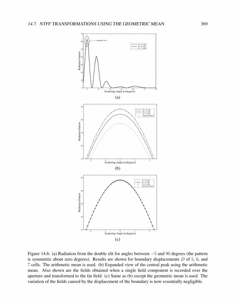
14.7. NTFF TRANSFORMATIONS USING THE GEOMETRIC MEAN 369
0 15 30 45 60 75 90
Scattering Angle φ [degrees]
0
10
20
30
40
50
60
70
Rad
iati
on P
atte
rn
D = 5 cellsD = 6 cellsD = 7 cells
expanded view
(a)
-2 -1 0 1 2
Scattering Angle φ [degrees]
45
50
55
60
65
Rad
iati
on
Pat
tern
D = 5 cellsD = 6 cellsD = 7 cellsAperture-Based
(b)
-2 -1 0 1 2
Scattering Angle φ [degrees]
45
50
55
60
65
Rad
iati
on
Pat
tern
D = 5 cellsD = 6 cellsD = 7 cellsAperture-Based
(c)
Figure 14.6: (a) Radiation from the double slit for angles between −5 and 90 degrees (the patternis symmetric about zero degrees). Results are shown for boundary displacements D of 5, 6, and7 cells. The arithmetic mean is used. (b) Expanded view of the central peak using the arithmeticmean. Also shown are the fields obtained when a single field component is recorded over theaperture and transformed to the far field. (c) Same as (b) except the geometric mean is used. Thevariation of the fields caused by the displacement of the boundary is now essentially negligible.

370 CHAPTER 14. NEAR-TO-FAR-FIELD TRANSFORMATION
x
y
z
incident
plane wave
circular scatterer
radius = 8
TFSFboundary
integrationboundary
Figure 14.7: Geometry of the circular PEC cylinder.
fields on the integration boundary. The variation between these peaks is less than 0.022, i.e., areduction in variation by a factor of approximately 270. This demonstrates that, unlike with thearithmetic mean, the location of the integration boundary is effectively irrelevant when using theGM-NTFF transform.
Naturally, at finer discretizations, the difference between the geometric mean and the arithmeticmean are less dramatic, but the geometric mean consistently performs better than the arithmeticmean.
(Simpson’s rule was used for all integrations except for the integration of the aperture fieldswhere a Riemann sum was used.)
14.7.2 Scattering from a Circular CylinderConsider scattering from a PEC circular cylinder under TMz polarization as shown in Fig. 14.7.The Dey-Mittra scheme is employed to help reduce the effects of staircasing [2]. The cylinder haseight cells along its radius. A pulsed plane wave which travels in the x direction is introduced viaa TFSF boundary. The simulation is run 512 time steps. Because the Dey-Mittra scheme is used,the Courant number was reduced to approximately 35 percent of the 2D limit in order to ensurestability [3].
Figure 14.8 shows the wavelength-normalized scattering width of the cylinder as a function ofscattering angle obtained using the series solution for a circular cylinder [4], the arithmetic-meanNTFF transform, and the GM-NTFF transform. (The normalized scattering width is the same asthe radiation pattern given in (14.87) where ρ is now taken to be the distance from the center of thecylinder.) The discretization is such that there are 9.92526 cells per wavelength at the frequencybeing considered here. One should keep in mind that the discretization of the cylinder introducessome errors and hence the “exact” solution for a circular cylinder is not truly exact for the scatterer

14.7. NTFF TRANSFORMATIONS USING THE GEOMETRIC MEAN 371
0 15 30 45 60 75 90 105 120 135 150 165 180
Scattering Angle φ [degrees]
1
10
Sca
tter
ing
Wid
th σ
2D
/λ
ExactArithmetic MeanGeometric Mean
Figure 14.8: Scattering width of a circular cylinder. The radius is eight cells and the frequencycorresponds to 9.92526 cells per wavelength.
present in the simulation. Therefore, the reference solution does not provide a perfect way withwhich to judge the solutions. Nevertheless, one hopes that the FDTD scatterer, when employingthe Dey-Mittra scheme, is a close approximation to a true circular scatterer and thus the exactsolution from the continuous world provides a reasonable basis for comparison.
The difference between the solutions in Fig. 14.8 are seen to be relatively small. Figure 14.9shows a plot of the magnitude of the difference between the exact solution and the FDTD-basedsolutions. Although there are angles where the arithmetic mean performs better than the geometricmean, in general the geometric mean is better. The integrated error for angles between 0 and π is0.6936 for the arithmetic mean and 0.3221, i.e., the error is reduced by more than a factor of twoby using the geometric mean.
14.7.3 Scattering from a Strongly Forward-Scattering SphereFinally, consider scattering from a dielectric sphere, depicted in Fig. 14.10, which has a relativepermittivity εr of 1.21. Such a sphere was considered in [5] and can also be found in Sec. 8.7 of[6]. In this case the transformation traditionally entails finding the tangential fields over the sixsides of a cuboid which bounds the sphere. The sphere is discretized such that there are 60 cellsalong the radius. A staircase representation is used (where a node is simply either inside or outsidethe sphere). The simulation is run at 95 percent of the 3D Courant limit (0.95/
√3) for 2048 time
steps. The grid is terminated with an eight-cell perfectly-matched layer.Figure 14.11 shows the normalized scattering cross section as a function of the equatorial angle
φ. The frequency corresponds to 20.06 cells per wavelength. The exact solution was obtained viathe Mie series (see, e.g., [7]). As was the case in 2D, both the arithmetic and geometric meanperform reasonably well, but the geometric mean is generally more accurate than the arithmeticmean. In Fig. 14.11 visible errors are only present near the back-scattering direction of φ = 180

372 CHAPTER 14. NEAR-TO-FAR-FIELD TRANSFORMATION
0 15 30 45 60 75 90 105 120 135 150 165 180
Scattering Angle φ [degrees]
0
0.2
0.4
0.6
0.8
1
Err
or
Mag
nit
ud
eArithmetic MeanGeometric Mean
Figure 14.9: Magnitude of the difference between the FDTD-based solutions and the nominallyexact solution.
y
x
z
Hi=Hy ay
^
Ei=Ez az
^
ki=kx ax
^
φ
i
i
i
Figure 14.10: Geometry of the dielectric sphere. The relative permittivity εr is 1.21. This incidentfield is polarized in the z direction and travels in the x direction. The equatorial angle φ is in thexy-plane with φ = 0 corresponding to the +x direction.

14.7. NTFF TRANSFORMATIONS USING THE GEOMETRIC MEAN 373
0 15 30 45 60 75 90 105 120 135 150 165 180
Equatorial angle φ [degrees]
0.0001
0.001
0.01
0.1
1
10
100
1000
Norm
aliz
ed c
ross
sec
tion σ
/λ2
ExactArithmetic meanGeometric mean
Figure 14.11: Scattering cross section of a dielectric sphere versus the equatorial angle φ. Thesphere is discretized with 60 cells along the radius and the frequency used here corresponds to20.06 cells per wavelength.
degrees. Note that there is a large difference, approximately five orders of magnitude, between thescattering in the forward and backward directions.
In order to improve the results in the back-scattering direction Li et al. [5] advocated calculatingthe transformation using the five faces other than the forward-scattering face. Figure 14.12 showsthe normalized backscattering cross section versus wavelength (expressed in terms of number ofcells per wavelength) calculated using the arithmetic mean. The normalized cross section is givenby
1
λ2limr→∞
[4πr2 |Ez(θ, φ)|2
|Eiz|2
](14.88)
where r is the distance from the center of the sphere, θ is the azimuthal angle and φ is the equatorialangle. For backscatter, θ is π/2 and φ is π.
The NTFF transform results shown in Fig. 14.12 were calculated using either the fields overall six faces of the integration boundary or the fields over the five faces advocated by Li et al. Theresults in this figure correspond to those shown in Fig. 1(b) of [5] for the sphere with a radiusof 3 µm. (However, for the sake of generality, here the results are plotted in terms of unitlessquantities.) Note that the six-sided arithmetic-mean results presented here are better than thosepresented in [5]. We were able to duplicate the results presented in [5] by not applying a temporalphase-correction factor (or, similarly, by applying a correction factor which is twice the factorgiven here). Nevertheless, the recommendation of Li et al. is true that the five-sided computation

374 CHAPTER 14. NEAR-TO-FAR-FIELD TRANSFORMATION
20 25 30 35 40
Cells per wavelength
0.01
0.1
1
Norm
aliz
ed b
acksc
atte
ring c
ross
sec
tion σ
b/λ
2ExactArithmetic, 6-sided transform
Arithmetic, 5-sided transform
Figure 14.12: Backscatter from a sphere with εr = 1.21 versus the wavelength (expressed in termsof number of cells). The FDTD transformations are calculated using the arithmetic mean and eithera five- or six-sided transformation boundary.
is better than the six-sided one for calculating the backscattering when using the arithmetic mean.However, for directions other than backscatter or for other sizes, one does not know a priori if aface should or should not be discarded.
Figure 14.13 is the same as Fig. 14.12 except the transformation is done using the GM-NTFFtransform. In this case discarding data from the forward-scattering face actually slightly degradesthe quality of the transform. Thus, when using the geometric mean there is no need to discard data.One can use it confidently for all scattering angles and all sizes.
To summarize, unlike the traditional arithmetic mean, for a single harmonic plane wave thegeometric mean accounts for the spatial offset of the fields in a way that is exact. In practice,where a spectrum of wave vectors are present, the geometric mean typically performs significantlybetter than the arithmetic mean. The geometric mean is much less sensitive to the integration-boundary location than is the arithmetic mean. For strongly forward-scattering objects, the useof the geometric mean obviates the need to discard the fields over the forward face (as has beenadvocated previously) when calculating the backscatter. The geometric mean does entail a slightincrease in computational cost because for each node along the integration boundary a DFT mustbe calculated for three fields instead of two. However, this cost is typically minor compared to theoverall simulation cost.

14.7. NTFF TRANSFORMATIONS USING THE GEOMETRIC MEAN 375
20 25 30 35 40
Cells per wavelength
0.001
0.01
0.1
1
Norm
aliz
ed b
acksc
atte
ring c
ross
sec
tion σ
b/λ
2
ExactGeometric, 6-sided
Geometric, 5-sided transform
Figure 14.13: Backscatter from a sphere with εr = 1.21 versus the wavelength (expressed in termsof number of cells). The transformations use the geometric mean and the fields over either five orsix faces of the integration boundary.

.376 CHAPTER 14. NEAR-TO-FAR-FIELD TRANSFORMATION

Appendix A
Construction of Fourth-Order CentralDifferences
Assuming a uniform spacing of δ between sample points, we seek an approximation of the deriva-tive of a function at x0 which falls midway between two sample point. Taking the Taylor seriesexpansion of the function at the four sample points nearest to x0 yields
f
(x0 +
3δ
2
)= f(x0) +
3δ
2f ′(x0) +
1
2!
(3δ
2
)2
f ′′(x0) +1
3!
(3δ
2
)3
f ′′′(x0) + . . . , (A.1)
f
(x0 +
δ
2
)= f(x0) +
δ
2f ′(x0) +
1
2!
(δ
2
)2
f ′′(x0) +1
3!
(δ
2
)3
f ′′′(x0) + . . . , (A.2)
f
(x0 −
δ
2
)= f(x0)− δ
2f ′(x0) +
1
2!
(δ
2
)2
f ′′(x0)− 1
3!
(δ
2
)3
f ′′′(x0) + . . . , (A.3)
f
(x0 −
3δ
2
)= f(x0)− 3δ
2f ′(x0) +
1
2!
(3δ
2
)2
f ′′(x0)− 1
3!
(3δ
2
)3
f ′′′(x0) + . . . (A.4)
Subtracting (A.3) from (A.2) and (A.4) from (A.1) yields
f
(x0 +
δ
2
)− f
(x0 −
δ
2
)= δf ′(x0) +
2
3!
(δ
2
)3
f ′′′(x0) + . . . (A.5)
f
(x0 +
3δ
2
)− f
(x0 −
3δ
2
)= 3δf ′(x0) +
2
3!
(3δ
2
)3
f ′′′(x0) + . . . (A.6)
The goal now is to eliminate the term containing f ′′′(x0). This can be accomplished by multiplying(A.5) by 27 and then subtracting (A.6). The result is
27f
(x0 +
δ
2
)− 27f
(x0 −
δ
2
)− f
(x0 +
3δ
2
)+ f
(x0 −
3δ
2
)= 24δf ′(x0) +O(δ5). (A.7)
Solving for f ′(x0) yields
df(x)
dx
∣∣∣∣x=x0
=9
8
f(x0 + δ
2
)− f
(x0 − δ
2
)δ
− 1
24
f(x0 + 3δ
2
)− f
(x0 − 3δ
2
)δ
+O(δ4). (A.8)
A.377

A.378 APPENDIX A. CONSTRUCTION OF FOURTH-ORDER CENTRAL DIFFERENCES
The first term on the right-hand side is the contribution from the sample points nearest x0 and thesecond term is the contribution from the next nearest points. The highest-order term not shown isfourth-order in terms of δ.

Appendix B
Generating a Waterfall Plot and Animation
Assume we are interested in plotting multiple snapshots of one-dimensional data. A waterfall plotdisplays all the snapshots in a single image where each snapshot is offset slightly from the next.On the other hand, animations display one image at a time, but cycle through the images quicklyenough so that one can clearly visualize the temporal behavior of the field. Animations are awonderful way to ascertain what is happening in an FDTD simulation but, since there is no way toput an animation on a piece of paper, waterfall plots also have a great deal of utility.
We begin by discussing waterfall plots. First, the data from the individual frames must beloaded into Matlab. The m-file for a function to accomplish this is shown in Program B.1. Thisfunction, readOneD(), reads each frame and stores the data into a matrix—each row of whichcorresponds to one frame. readOneD() takes a single argument corresponding to the base nameof the frames. For example, issuing the command z = readOneD(’sim’); would create amatrix z where the first row corresponded to the data in file sim.0, the second row to the data infile sim.1, and so on.
Note that there is a waterfall() function built into Matlab. One could use that to displaythe data by issuing the command waterfall(z). However, the built-in command is arguablyoverkill. Its hidden-line removal and colorization slow the rendering and do not necessarily aide inthe visualization of the data.
The plot shown in Fig. 3.9 did not use Matlab’s waterfall() function. Instead, it wasgenerated using a function called simpleWaterfall() whose m-file is shown in ProgramB.2. This command takes three arguments. The first is the matrix which would be created byreadOneD(), the second is the vertical offset between successive plots, and the third is a verticalscale factor.
Given these two m-files, Fig. 3.9 was generated using the following commands:
z = readOneD(’sim’);simpleWaterfall(z, 1, 1.9) % vertical offset = 1, scale factor = 1.9xlabel(’Space [spatial index]’)ylabel(’Time [frame number]’)
Program B.1 readOneD.m Matlab code to read one-dimensional data from a series of frames.
B.379

B.380 APPENDIX B. GENERATING A WATERFALL PLOT AND ANIMATION
1 function z = readOneD(basename)2 %readOneD(BASENAME) Read 1D data from a series of frames.3 % [Z, dataLength, nFrames] = readOneD(BASENAME) Data4 % is read from a series of data files all which have5 % the common base name given by the string BASENAME,6 % then a dot, then a frame index (generally starting7 % with zero). Each frame corresponds to one row of Z.8
9 % read the first frame and establish length of data10 nFrames = 0;11 filename = sprintf(’%s.%d’, basename, nFrames);12 nFrames = nFrames + 1;13 if exist(filename, ’file’)14 z = dlmread(filename, ’\n’);15 dataLength = length(z);16 else17 return;18 end19
20 % loop through other frames and break out of loop21 % when next frame does not exist22 while 123 filename = sprintf(’%s.%d’,basename,nFrames);24 nFrames = nFrames + 1;25 if exist(filename, ’file’)26 zTmp = dlmread(filename, ’\n’);27 if length(zTmp) ˜= dataLength % check length matches28 error(’Frames have different sizes.’)29 break;30 end31 z = [z zTmp]; % append new data to z32 else33 break;34 end35 end36
37 % reshape z to appropriate dimensions38 z = reshape(z, dataLength, nFrames - 1);39 z = z’;40
41 return;
Program B.2 simpleWaterfall.m Matlab function to generate a simple waterfall plot.

B.381
1 function simpleWaterfall(z, offset, scale)2 %simpleWaterfall Waterfall plot from offset x-y plots.3 % simpleWaterfall(Z, OFFSET, SCALE) Plots each row of z4 % where successive plots are offset from each other by5 % OFFSET and each plot is scaled vertically by SCALE.6
7 hold off % release any previous plot8 plot(scale * z(1, :)) % plot the first row9 hold on % hold the plot
10
11 for i = 2:size(z, 1) % plot the remaining rows12 plot(scale * z(i, :) + offset * (i - 1))13 end14
15 hold off % release the plot16
17 return
A function to generate an animation of one-dimensional data sets is shown in Program B.3.There are multiple ways to accomplish this goal and thus one should keep in mind that ProgramB.3 is not necessarily the best approach for a particular situation. The function in Program B.3is called oneDmovie() and it takes three arguments: the base name of the snapshots, and theminimum and maximum values of the vertical axis. The function uses a loop, starting in line25, to read each of the snapshots. Each snapshot is plotted and the plot recorded as a frame of aMatlab “movie” (see the Matlab command movie() for further details). The oneDmovie()function returns an array of movie frames. As an example, assume the base name is “sim” andthe user wants the plots to range from −1.0 to 1.0. The following commands would display theanimation 10 times (the second argument to the movie() command controls how often the movieis repeated):
reel = oneDmovie(’sim’,-1,1);movie(reel,10)
An alternative implementation might read all the data first, as was done with the waterfall plot, andthen determine the “global” minimum and maximum values from the data itself. This would freethe user from specify those value as oneDmovie() currently requires. Such an implementationis left to the interested reader.
Program B.3 oneDmovie.m Matlab function which can be used to generate an animation formultiple one-dimensional data sets. For further information on Matlab movies, see the Matlabcommand movie.
1 function reel = oneDmovie(basename, y_min, y_max)2 % oneDmovie Create a movie from data file with a common base3 % name which contain 1D data.

B.382 APPENDIX B. GENERATING A WATERFALL PLOT AND ANIMATION
4 %5 % basename = common base name of all files6 % y_min = minimum value used for all frames7 % y_max = maximum value used for all frames8 %9 % reel = movie which can be played with a command such as:
10 % movie(reel, 10)11 % This would play the movie 10 times. To control the frame12 % rate, add a third argument specifying the desired rate.13
14 % open the first frame (i.e., first data file).15 frame = 1;16 filename = sprintf(’%s.%d’, basename, frame);17 fid = fopen(filename, ’rt’);18
19 % to work around rendering bug under Mac OS X see:20 % <www.mathworks.com/support/solutions/21 % data/1-VW0GM.html?solution=1-VW0GM>22 figure; set(gcf, ’Renderer’, ’zbuffer’);23
24 % provided fid is not -1, there is another file to process25 while fid ˜= -126 data=fscanf(fid, ’%f’); % read the data27 plot(data) % plot the data28 axis([0 length(data) y_min y_max]) % scale axes appropriately29 reel(frame) = getframe; % capture the frame for the movie30
31 % construct the next file name and try to open it32 frame = frame + 1;33 filename = sprintf(’%s.%d’, basename, frame);34 fid = fopen(filename, ’rb’);35 end36
37 return

Appendix C
Rendering and Animating Two-DimensionalData
The function shown below is Matlab code that can be used to generate a movie from a sequenceof binary (raw) files. The files (or frames) are assumed to be named such that they share a com-mon base name then have a dot followed by a frame number. Here the frame number is assumedto start at zero. The function can have one, two, or three arguments. This first argument is thebase name, the second is the value which is used to normalize all the data, and the third argumentspecifies the number of decades of data to display. Here the absolute value of the data is plottedin a color-mapped imaged. Logarithmic (base 10) scaling is used so that the value which is nor-malized to unity will correspond to zero on the color scale and the smallest normalized value willcorrespond, on the color scale, to the negative of the number of decades (e.g., if the number ofdecades were three, the smallest value would correspond to −3). This smallest normalized valueactually corresponds to a normalized value of 10−d where d is the number of decades. Thus the(normalized) values shown in the output varying from 10−d to 1. The default normalization andnumber of decades are 1 and 3, respectively.
Program C.1 raw2movie.m Matlab function to generate a movie given a sequence of raw files.
1 function reel = raw2movie(basename, z_norm, decades)2 % raw2movie Creates a movie from "raw" files with a common base3 % name.4 %5 % The absolute value of the data is used together with6 % logarithmic scaling. The user may specify one, two, or7 % three arguments.8 % raw2movie(basename, z_norm, decades) or9 % raw2movie(basename, z_norm) or
10 % raw2movie(basename):11 % basename = common base name for all files12 % z_norm = value used to normalize all frames, typically this13 % would be the maximum value for all the frames.
C.383

C.384 APPENDIX C. RENDERING AND ANIMATING TWO-DIMENSIONAL DATA
14 % Default value is 1.15 % decades = decades to be used in the display. The normalized16 % data is assumed to vary between 1.0 and 10ˆ(-decades)17 % so that after taking the log (base 10), the values18 % vary between 0 and -decades. Default value is 3.19 %20 % return value:21 % reel = movie which can be played with a command such as:22 % movie(reel, 10)23 % pcolor() is used to generate the frames.24 %25 % raw file format:26 % The raw files are assumed to consist of all floats (in27 % binary format). The first two elements specify the horizontal28 % and vertical dimensions. Then the data itself is given in29 % English book-reading order, i.e., from the upper left corner30 % of the image and then scanned left to right. The frame number31 % is assumed to start at zero.32
33 % set defaults if we have less than three arguments34 if nargin < 3, decades = 3; end35 if nargin < 2, z_norm = 1.0; end36
37 % open the first frame38 frame = 0;39 filename = sprintf(’%s.%d’, basename, frame);40 fid = fopen(filename, ’rb’);41
42 if fid == -143 error([’raw2movie: initial frame not found: ’, filename])44 end45
46 % to work around rendering bug under Mac OS X implementation.47 figure; set(gcf, ’Renderer’, ’zbuffer’);48
49 % provided fid is not -1, there is another file to process50 while fid ˜= -151 size_x = fread(fid, 1, ’single’);52 size_y = fread(fid, 1, ’single’);53
54 data = flipud(transpose(...55 reshape(...56 fread(fid, size_x * size_y, ’single’), size_x, size_y)...57 ));58
59 % plot the data60 if decades ˜= 0

C.385
61 pcolor(log10(abs((data + realmin) / z_norm)))62 shading flat63 axis equal64 axis([1 size_x 1 size_y])65 caxis([-decades 0])66 colorbar67 else68 pcolor(abs((data + realmin) / z_norm))69 shading flat70 axis equal71 axis([1 size_x 1 size_y])72 caxis([0 1])73 colorbar74 end75
76 % capture the frame for the movie (Matlab wants index to start77 % at 1, not zero, hence the addition of one to the frame)78 reel(frame + 1) = getframe;79
80 % construct the next file name and try to open it81 frame = frame + 1;82 filename = sprintf(’%s.%d’, basename, frame);83 fid = fopen(filename,’ rb’);84
85 end

C.386 APPENDIX C. RENDERING AND ANIMATING TWO-DIMENSIONAL DATA

Appendix D
Notation
c speed of light in free spaceNfreq index of spectral component corresponding to a frequency with discretization Nλ
Nλ number of points per wavelength for a given frequency(the wavelength is the one pertaining to propagation in free space)
NL number of points per skin depth (L for loss)NP number of points per wavelength at peak frequency of a Ricker waveletNT number of time steps in a simulationSc Courant number (c∆t/∆x in one dimension)st Temporal shift operatorsx Spatial shift operator (in the x direction)
D.387

D.388 APPENDIX D. NOTATION

Appendix E
PostScript Primer
E.1 IntroductionPostScript was developed by Adobe Systems Incorporated and is both a page-description languageand a programming language. Unlike a JPEG or GIF file which says what each pixel in an imageshould be, PostScript is “vector based” and thus a PostScript file specifies graphic primitives, suchas lines and arcs. There primitives are described by various PostScript commands. The quality ofthe image described by a PostScript file will depend on the output device. For example, a laserprinter with 1200 dots per inch will draw a better curved line than would a laser printer with 300dots per inch (although both will typically produce very good output).
The goal here is to show how one can easily generate PostScript files which convey informa-tion about an FDTD simulation. Thus we are more interested in the page-description aspects ofPostScript rather than its programming capabilities. (There is a wonderful book and Web site byBill Casselman that describe PostScript extremely well while illustrating a host of mathematicalconcepts. The book is entitled Mathematical Illustrations: A Manual of Geometry and PostScriptwhich you can find at www.math.ubc.ca/˜cass/graphics/manual/. It is well worthchecking out.)
PostScript is a Forth-like language in that it uses what is known as postfix notation. If you haveused an RPN (reverse Polish notation) calculator, you are familiar with postfix notation. You putarguments onto a “stack” and then select an operation which “pops” the arguments from the stackand operates on them. For example, to add 3 and 12 you would enter the following:
3<ENTER>12+
When 3 is typed on the keypad, it is placed at the top of the stack. It is pushed onto the next stacklocation by hitting the ENTER key. When 12 is typed, it is put at the top of the stack. Hitting theplus sign tells the calculator you want to add the top two numbers on the stack, i.e., the 3 and 12.These numbers are popped (i.e., taken) from the stack, and the result of the addition (15) is placedat the top of the stack.
Lecture notes by John Schneider. postscript-primer.tex
E.389

E.390 APPENDIX E. POSTSCRIPT PRIMER
The PostScript language is much like this. Arguments are given before the operations. Giv-ing arguments before operations facilitates the construction of simple interpreters. PostScript in-terpreters typically have the task of translating the commands in a PostScript file to some formof viewable graphics. For example, there are PostScript printers which translate (interpret) aPostScript file into a printed page. Most computers have PostScript interpreters which permitthe graphics described in a PostScript file to be displayed on the screen. There are free PostScriptinterpreters available via the Web (you should do a search for GhostScript if you are in need of aninterpreter).
E.2 The PostScript FileA file which contains PostScript commands, which we will call a PostScript file, is a plain ASCIIfile which must start with “%!PS”. These characters are often referred to as a “magic word.”Magic words appear at the start of many computer files and identify the contents of the file. This%!PS magic word identifies the contents of the file as PostScript to the interpreter. (The names ofPostScript file often end with the suffix .ps, but the interpreter does not care what the file nameis.) The last command in a PostScript file is typically showpage. This command essentially tellsthe interpreter that all the commands have been given and the page (or screen image or whatever)should be rendered.
What comes between %!PS and showpage are the commands which specify how the pageshould appear. Before exploring some of these commands it is important to know that a PostScriptinterpreter, by default, thinks in terms of units of “points” which are not points in the geometricsense, but rather 1/72 of an inch. Points are a traditional unit used in the printing industry (thus a“12-point font” is one for which a typical capital letter is 12/72 of an inch high). A default “page”is 8.5 by 11 inches and thus 612 by 792 points. The origin is the lower left corner of the page.
E.3 PostScript Basic CommandsThe PostScript command moveto takes two arguments: the x and y coordinates to which thecurrent point should be moved. You can think of the current point as akin to the point where the tipof a pen is moved. To define a line we can give the command lineto. lineto also takes twoarguments: the x and y coordinates of the point to which the line should be drawn. In PostScript,after issuing the lineto command we have merely defined the path of the line—we have notactually drawn anything yet. You can think of this as the pen having drawn the line in invisible ink.We have to issue one more command to make the line visible, the stroke command.
A complete PostScript file (which we will identify as a “Program”) which draws a line fromthe point (100, 200) to the point (300, 600) is shown in Program E.1.
Program E.1 PostScript commands to draw a single tilted line.
%!PS100 200 moveto

E.3. POSTSCRIPT BASIC COMMANDS E.391
(0,0)
(0,796)
(612,0)
(612,796)
Figure E.1: Simple line rendered by the PostScript commands giving in Program E.1 and E.2. Thesurrounding box and corner labels have been added for the sake of clarity.
300 600 linetostrokeshowpage
The image drawn by these commands is shown in Fig. E.1. The surrounding border and coordinatelabels have been added for clarity. The only thing which would actually be rendered is the tiltedline shown within the border.
Instead of using the command lineto to specify the point to which we want the line tobe drawn, the command rlineto can be used where now the arguments specify the relativemovement from the current point (hence the “r” for relative). The arguments of rlineto specifythe relative displacement from the current point. In the commands in Program E.1, the line whichwas drawn went 200 points in the x direction and 400 points in the y direction from the startingpoint. Thus instead of writing 300 600 lineto, one could obtain the same result using 200400 rlineto. PostScript does not care about whitespace and the percent sign is used to indicatethe start of a comment (the interpreter ignores everything from the percent sign to the end of theline). Thus, another file which would also yield the output shown in Fig. E.1 is shown in ProgramE.2. (The magic word must appear by itself on the first line of the file.)
Program E.2 PostScript commands to draw a single tilted line. Here the rlineto command isused. The resulting image is identical to the one produced by Progam E.1 and is shown in Fig. E.1.

E.392 APPENDIX E. POSTSCRIPT PRIMER
%!PS% tilted line using the rlineto command100 200 moveto 300 600 lineto stroke showpage
When creating graphics it is often convenient to redefine the origin of the coordinate system toa point which is more natural to the object being drawn. PostScript allows us to translate the originto any point on the page using the translate command. This command also takes two argu-ments corresponding to the point in the current coordinate system where the new origin should belocated. For example, let us assume we want to think in terms of both positive and negative coor-dinates. Therefore we wish to place the origin in the middle of the page. This can be accomplishedwith the command 306 396 translate. The PostScript commands shown in Program E.3demonstrate the use of the translate command.
Program E.3 PostScript commands which first translate the origin to the center of the page andthen draw four lines which “radiate away” from the origin. The corner labels show the cornercoordinates after the translation of the origin to the center of the page.
%!PS306 398 translate % translate origin to center of page100 100 moveto 50 50 rlineto stroke-100 100 moveto -50 50 rlineto stroke-100 -100 moveto -50 -50 rlineto stroke100 -100 moveto 50 -50 rlineto strokeshowpage
Program E.3 yields the results shown in Fig. E.2.As you might imagine, thinking in terms of units of points (1/72 of an inch) is not always
convenient. PostScript allows us to scale the dimensions by any desired value using the scalecommand. In fact, one can use a different scale factor in both the x and the y directions and thusscale takes two arguments. However, we will stick to using equal scaling in both directions.
In the previous example, all the locations were specified in terms of multiples of 50. Thereforeit might make sense to scale the dimensions by a factor of 50 (in both the x and y direction). Thisscaling should be done after the translation of the origin. We might anticipate that the commandsshown in Program E.4 would render the same output as shown in Fig. E.2.
Program E.4 PostScript file where the units are scaled by a factor of 50 in both the x and ydimensions.

E.3. POSTSCRIPT BASIC COMMANDS E.393
(-306,-398)
(-306,398)
(306,-398)
(306,398)
Figure E.2: Output rendered by Program E.3 which translates the origin to the center of the page.This output is also produced by Program E.5 and Program E.6.
%!PS306 398 translate50 50 scale % scale units in x and y direction by 502 2 moveto 1 1 rlineto stroke-2 2 moveto -1 1 rlineto stroke-2 -2 moveto -1 -1 rlineto stroke2 -2 moveto 1 -1 rlineto strokeshowpage
However this file yields the output shown in Fig. E.3. Note that the lines which radiate from originare now much thicker. In fact, they are 50 times thicker than they were in the previous image. Bydefault, a line in PostScript has a thickness of unity i.e., one point. The scale command scaledthe line thickness along with all the other dimensions so that now the line thickness is 50 points.
Although we have only given integer dimensions so far, as far as PostScript is concerned allvalues are actually real numbers (i.e., floating-point numbers). We can control the line thicknesswith the setlinewidth command which takes a single argument. If we want the line thicknessstill to be one point, the line thickness should be set to the inverse of the scale factor, i.e., 1/50 =0.02. Also, it is worth noting that the stroke command does not have to be given after each drawingcommand. We just have to ensure that it is given before the end of the file (or before the line stylechanges to something else). Thus, a PostScript file which scales the dimensions by 50 and producesthe same output as shown in Fig. E.2 is shown in Program E.4

E.394 APPENDIX E. POSTSCRIPT PRIMER
(-306,-398)
(-306,398)
(306,-398)
(306,398)
Figure E.3: Output rendered by Program E.4 which scales the units by 50.
Program E.5 PostScript file where the units are scaled by a factor of 50 and the line thickness iscorrected to account for this scaling. Note that a single stroke command is given.
%!PS306 398 translate50 50 scale0.02 setlinewidth % correct line thickness to account for scaling2 2 moveto 1 1 rlineto-2 2 moveto -1 1 rlineto-2 -2 moveto -1 -1 rlineto2 -2 moveto 1 -1 rlineto strokeshowpage
PostScript permits the use of named variables and, as we shall see, named procedures. Thisis accomplished using the def command which takes, essentially, two arguments: the first beingthe literal string which is the variable or procedure name and the second being the value or proce-dure (where the procedure would be enclosed in braces). A literal string is a backslash characterfollowed by the string. For example, the following sets the variable scalefactor to 50:
/scalefactor 50 def
After issuing this command, we can use scalefactor in place of 50 everywhere in the file.The PostScript language includes a number of mathematical functions. One can add using
add, subtract using sub, multiply using mul, and divide using div. Each of these functions

E.3. POSTSCRIPT BASIC COMMANDS E.395
takes two arguments consistent with an RPN calculator. To calculate the inverse of 50, one couldissue the following command:
1 50 div
This places 1 on the stack, then 50, and then divides the two. The result, 0.02, remains at the topof the stack.
The program shown in Program E.6 uses the def and div commands and is arguably a bitcleaner and better self-documenting than the one shown in Program E.5. Program E.6 also pro-duces the output shown in Fig. E.2.
Program E.6 PostScript file which uses the def command to define a scale-factor which is setto 50. The inverse of the scale-factor is obtained by using the div command to divide 1 by thescale-factor.
%!PS306 398 translate% define "scalefactor" to be 50/scalefactor 50 def% scale x and y directions by the scale factorscalefactor scalefactor scale% set line width to inverse of the scale factor1 scalefactor div setlinewidth2 2 moveto 1 1 rlineto-2 2 moveto -1 1 rlineto-2 -2 moveto -1 -1 rlineto2 -2 moveto 1 -1 rlineto strokeshowpage
The arc command takes five arguments: the x and y location of the center of the arc, theradius of the arc, and the angles (in degrees) at which the arc starts and stops. For example, thefollowing command would draw a complete circle of radius 0.5 about the point (2, 2):
2 2 0.5 0 360 arc stroke
Let us assume we wish to draw several circles, each of radius 0.5. We only wish to change thecenter of the circle. Rather than specifying the arc command each time with all its five arguments,we can use the def command to make the program more compact. Consider the program shownin Program E.7. Here the def command is used to say that the literal circle is equivalent to0.5 0 360 arc stroke, i.e., three of the arguments are given to the arc command—onejust has to provide the two missing arguments which are the x and y location of the center of thecircle. The output produced by this program is shown in Fig. E.4.

E.396 APPENDIX E. POSTSCRIPT PRIMER
(-306,-398)
(-306,398)
(306,-398)
(306,398)
Figure E.4: Output rendered by Program E.7.
Program E.7 PostScript file which renders the output shown in Fig. E.4.
%!PS306 398 translate/scalefactor 50 defscalefactor scalefactor scale1 scalefactor div setlinewidth/circle 0.5 0 360 arc stroke def2 2 circle-2 2 circle-2 -2 circle2 -2 circleshowpage
In addition to stroke-ing a path, PostScript allows paths to be fill-ed using the fill com-mand. So, instead of drawing a line around the perimeter of the circles shown in Fig. E.4, one canobtain filled circles by issuing the fill command instead of the stroke command. ProgramE.8 and the corresponding output shown in Fig. E.5 illustrate this.
Program E.8 PostScript file which defines a stroke-ed and fill-ed circle. The correspondingoutput is shown in Fig. E.5.

E.3. POSTSCRIPT BASIC COMMANDS E.397
(-306,-398)
(-306,398)
(306,-398)
(306,398)
Figure E.5: Output rendered by Program E.8.
%!PS306 398 translate/scalefactor 50 defscalefactor scalefactor scale1 scalefactor div setlinewidth/circle 0.5 0 360 arc stroke def/circlef 0.5 0 360 arc fill def2 2 circlef-2 2 circle-2 -2 circlef2 -2 circleshowpage
The PostScript commands we have considered are shown in Table E.1.Instead of using an editor to write a PostScript file directly, we can use another program to
generate the PostScript file for us. Specifically, let us consider a C program which generates aPostScript file. This program is supposed to demonstrate how one could use PostScript to displaya particular aspect of an FDTD grid. For example, let us assume we are using a TMz grid whichis 21 cells by 21 cells. There is a PEC cylinder with a radius of 5 which is centered in the grid.We know that the Ez nodes which fall within the cylinder should be set to zero and this zeroingoperation would be done with a for-loop. However, precisely which nodes are being set to zero?The code shown in Program E.9 could be incorporated into an FDTD program. This code producesthe PostScript output file grid.ps which renders the image shown in Fig. E.6. The first severallines of the file grid.ps are shown in Fragment E.10.

E.398 APPENDIX E. POSTSCRIPT PRIMER
Command Descriptionx y moveto move current point to (x, y)x y lineto draw a line from current point to (x, y)δx δy rlineto from current point draw a line over δx and up δyx y translate translate the origin to the point (x, y)sx sy scale scale x and y coordinates by sx and systroke “apply ink” to a previously defined pathfill fill the interior of a previously defined pathw setlinewidth set the line width to wd1 d2 div calculate d1/d2; result is placed at top of stackxc yc r a1 a2 arc draw an arc of radius r centered at (xc, yc)
starting at angle a1 and ending at angle a2 (degrees)/literal definition def define the literal string to have the given definition;
braces are needed if the definition contains any whitespace
Table E.1: An assortment of PostScript commands and their arguments.
Program E.9 C program which generates a PostScript file. The file draws either a cross or a filledcircle depending on whether a node is outside or inside a circular boundary, respectively. Therendered image is shown in Fig. E.6.
1 /* C program to generate a PostScript file which draws a cross2 * if a point is outside of a circular boundary and draws a3 * filled circle if the point is inside the boundary.4 */5
6 #include <stdio.h>7 #include <math.h>8
9 int is_inside_pec(double x, double y);10
11 int main() 12 int m, n;13
14 FILE *out;15
16 out = fopen("grid.ps","w"); // output file is "grid.ps"17
18 /* header material for PostScript file */19 fprintf(out,"%%!PS\n"20 "306 396 translate\n"21 "/scalefactor 20 def\n"22 "scalefactor scalefactor scale\n"23 "1 scalefactor div setlinewidth\n"

E.3. POSTSCRIPT BASIC COMMANDS E.399
24 "/cross moveto\n"25 " -.2 0 rmoveto .4 0 rlineto\n"26 " -.2 -.2 rmoveto 0 .4 rlineto stroke def\n"27 "/circle .2 0 360 arc fill def\n"28 );29
30 for (m=-10; m<=10; m++)31 for (n=-10; n<=10; n++)32 if (is_inside_pec(m,n)) 33 fprintf(out,"%d %d circle\n",m,n);34 else 35 fprintf(out,"%d %d cross\n",m,n);36 37
38 fprintf(out,"showpage\n");39
40 return 0;41 42
43 /* Function returns 1 if point (x,y) is inside a circle (or on44 * the perimeter of circle) and returns 0 otherwise.45 */46 int is_inside_pec(double x, double y) 47 double radius = 5.0;48
49 return x*x + y*y <= radius*radius;50
Fragment E.10 First several lines of the file grid.ps which is produced by Program E.9.
%!PS306 396 translate/scalefactor 20 defscalefactor scalefactor scale1 scalefactor div setlinewidth/cross moveto
-.2 0 rmoveto .4 0 rlineto-.2 -.2 rmoveto 0 .4 rlineto stroke def
/circle .2 0 360 arc fill def-10 -10 cross-10 -9 cross-10 -8 cross-10 -7 cross

E.400 APPENDIX E. POSTSCRIPT PRIMER
(-306,-398)
(-306,398)
(306,-398)
(306,398)
Figure E.6: Grid depiction rendered by the file grid.ps which is produced by Program E.9.Crosses corresponds to nodes which are outside a circular boundary of radius 5. Filled circlescorrespond to nodes inside the boundary (or identically on the perimeter of the boundary).

E.3. POSTSCRIPT BASIC COMMANDS E.401
-10 -6 cross...

402 APPENDIX E. POSTSCRIPT PRIMER

Bibliography
[1] D. Sullivan and J. L. Young. Far-field time-domain calculation from aperture radiators usingthe FDTD method. IEEE Transactions on Antennas and Propagation, 49(3):464–469, March2001.
[2] S. Dey and R. Mittra. A locally conformal finite-difference time-domain (FDTD) algorithmfor modeling three-dimensional perfectly conducting objects. IEEE Microwave Guided WaveLetters, 7(9):273–275, September 1997.
[3] S. Benkler, N. Chavannes, and N. Kuster. A new 3-D conformal PEC FDTD scheme with user-defined geometric precision and derived stability criterion. IEEE Transactions on Antennasand Propagation, 54(6):1843–1849, June 2006.
[4] C. A. Balanis. Advanced Engineering Electromagnetics. John Wiley & Sons, New York, 1989.
[5] X. Li, A. Taflove, and V. Backman. Modified FDTD near-to-far-field transformation for im-proved backscattering calculation of strongly forward-scattering objects. IEEE Antennas andWireless Propagation Letters, 4:35–38, 2005.
[6] A. Taflove and S. Hagness. Computational Electrodynamics: The Finite-Difference Time-Domain Method, 3 ed. Artech House, Boston, MA, 2005.
[7] A. Ishimaru. Electromagnetic Wave Propagation, Radiation, and Scattering. Prentice Hall,Englewood Cliffs, New Jersey, 1991.
403