1

Understanding Notions of Stationarity inNon-Smooth Optimization

Jiajin Li, Anthony Man-Cho So, Senior Member, IEEE, and Wing-Kin Ma, Fellow, IEEE

Abstract—Many contemporary applications in signal process-ing and machine learning give rise to structured non-convexnon-smooth optimization problems that can often be tackledby simple iterative methods quite effectively. One of the keysto understanding such a phenomenon—and, in fact, one of thevery difficult conundrums even for experts—lie in the study of“stationary points” of the problem in question. Unlike smoothoptimization, for which the definition of a stationary point israther standard, there is a myriad of definitions of stationarity innon-smooth optimization. In this article, we give an introductionto different stationarity concepts for several important classesof non-convex non-smooth functions and discuss the geometricinterpretations and further clarify the relationship among thesedifferent concepts. We then demonstrate the relevance of theseconstructions in some representative applications and how theycould affect the performance of iterative methods for tacklingthese applications.

Index Terms—non-smooth analysis, subdifferential, stationar-ity.

I. INTRODUCTION

In recent years, we have witnessed a fast-growing bodyof literature that utilizes non-convex non-smooth optimizationtechniques to tackle machine learning and signal processingapplications. Although such a development seems to runcontrary to the long-held belief that non-convex optimizationproblems pose serious analytic and algorithmic challenges,it is proven to be practically relevant and opens up anexciting avenue for dealing with contemporary applications.For instance, various low-rank matrix recovery problems ad-mit natural non-convex optimization formulations that canbe readily tackled by lightweight first-order methods (e.g.,(sub)gradient descent or block coordinate descent) and aremore scalable than their convex approximations; see, e.g., [1]–[5]. On the other hand, many modern statistical estimationproblems involve non-convex loss functions and/or regular-izers. While such problems are non-convex, they possesscertain convexity properties (which can be made precise) thatcan be exploited in computation, and there are algorithmsthat can compute solutions to these problems with goodempirical performance; see, e.g., [6]–[10]. Another examplethat has drawn immense interest is deep neural networks

This work is supported in part by the Hong Kong Research Grants Council(RGC) General Research Fund (GRF) projects CUHK 14208117 and CUHK14208819, and in part by the CUHK Research Sustainability of Major RGCFunding Schemes project 3133236.

J. Li and A. M.-C. So is with the Department of Systems Engineering andEngineering Management, The Chinese University of Hong Kong, Shatin,N.T., Hong Kong. E-mail: {jjli, manchoso}@se.cuhk.edu.hk.

W.-K. Ma is with the Department of Electronic Engineering, The ChineseUniversity of Hong Kong, Shatin, N.T., Hong Kong. E-mail: wkma@ieee.org.

with non-smooth activation functions (e.g., the rectified linearunit (ReLU) x 7→ max{x, 0}). To train such networks, oneoften needs to optimize a loss function that is recursivelydefined via compositions of linear mappings with nonlinearactivation functions. Despite the non-convexity and possi-ble non-smoothness of the loss function, various stochasticalgorithms (e.g., stochastic (sub)gradient descent or Adam-type algorithms) for optimizing it can still yield excitingempirical performance on a host of machine learning tasks;see, e.g., [11]–[13]. There are many other applications whosenatural optimization formulations are non-convex yet highlystructured, such as dictionary learning [14], [15], non-negativematrix factorization [16], [17], and phase retrieval [18], [19].It is becoming increasingly clear that by carefully exploitingthe structure of the non-convex formulation at hand, onecan design algorithms that have better empirical performanceand runtime than those for solving the corresponding convexapproximations.

To better understand such phenomenon, a general approachis to study the “stationary points” of the problem in questionand investigate how existing iterative methods behave aroundthese stationary points. For smooth optimization, the definitionof a stationary point is rather standard. Indeed, consider theunconstrained minimization problem

infx∈Rn

f(x) (1)

with f : Rn → R. Suppose that f is smooth and let ∇f :Rn → Rn be its gradient. A point x ∈ Rn is said to bestationary if

∇f(x) = 0,

which means that x is either a local minimum, a localmaximum, or a saddle point. However, for non-smooth op-timization, one can find a myriad of definitions of a stationarypoint in the literature; see, e.g., [20], [21] and the referencestherein. It is far from clear how these different definitionsof stationarity are related and, more fundamentally, whythey need to be introduced. This not only creates potentialconfusion among readers but also obscures the nature ofthe solutions that are being computed by different iterativemethods.

In this paper, our main objective is to give an introduc-tion to the theory of subdifferentiation for non-convex non-smooth functions, with a focus on motivating the differentconstructions of the subdifferential and developing the corre-sponding stationarity concepts for several important functionclasses, as well as discussing the geometric interpretationsand further clarifying the relationship among the different

2

constructions. We will also demonstrate the relevance of theseconstructions in some representative applications and howthey could affect the performance of iterative methods fortackling these applications. Readers may just be as intriguedby what classes of iterative algorithms can lead to efficientcomputation of a stationary point under the aforementionedconcepts. Unfortunately, owing to the need for exposition ofmore sophisticated concepts and also to the page limitation,we decide not to cover algorithms in this introductory article.

II. CONVEX NON-SMOOTH FUNCTIONS

To set the stage for our later developments, let us review thetheory of subdifferentiation for convex non-smooth functions.For simplicity, we restrict our discussion to finite-valuedconvex functions f : Rn → R. Recall that if f is convex andsmooth, then its gradient ∇f at x ∈ Rn provides an affineminorant of f at x ∈ Rn; i.e.,

f(y) ≥ f(x) +∇f(x)T (y − x) for all y ∈ Rn.

In the non-smooth case, a suitable generalization of gradient isthe notion of subgradient; i.e., a vector s ∈ Rn is a subgradientof f at x ∈ Rn if

f(y) ≥ f(x) + sT (y − x) for all y ∈ Rn.

Since the subgradient at a point may not be unique, we areled to the notion of subdifferential, which is the set

∂f(x) ={s ∈ Rn : f(y) ≥ f(x) + sT (y − x)

for all y ∈ Rn} . (2)

As it turns out, the subdifferential (2) can be constructedby considering the directional derivative of f . Given a pointx ∈ Rn and a direction d ∈ Rn, the difference quotient q off at x is defined by

t 7→ q(t) =f(x+ td)− f(x)

tfor t > 0. (3)

Observe that by the convexity of f , the function q is increasingin t (see, e.g., [22, Chapter 0, Proposition 6.1]) and boundedaround 0 (see, e.g., [22, Chapter B, Theorem 3.1.2]). Thus, thedirectional derivative of f at x ∈ Rn in the direction d ∈ Rn,which is defined by

f ′(x,d) = limt↘0

f(x+ td)− f(x)

t, (4)

exists and is equal to f ′(x,d) = inft>0 q(t). One of the keyproperties of f ′ is the following:

Fact 1 ( [22, Chapter D, Proposition 1.1.2]) For any x ∈ Rn,the function d 7→ f ′(x,d) is finite sublinear (recall that afunction h : Rn → R∪ {+∞} is sublinear if it is convex andsatisfies h(tx) = t · h(x) for all x ∈ Rn and t > 0).

A fundamental result in convex analysis is that there is acorrespondence between closed sublinear functions and closedconvex sets; see [22, Chapter C]. In particular, upon invok-ing [22, Chapter C, Theorem 3.1.1], we know that f ′(x, ·) isthe support function of the non-empty closed convex set

∂f(x) ={s ∈ Rn : sTd ≤ f ′(x,d) for all d ∈ Rn

}; (5)

i.e., f ′(x,d) = sups∈∂f(x) sTd. By the finiteness of f ′(x, ·),

the set ∂f(x) is bounded ( [22, Chapter C, Proposition 2.1.3]).Hence, ∂f(x) is in fact compact. It can be shown that (5)and (2) describe the same set; see [22, Chapter D, Theorem1.2.2]. Interestingly, even though we define the set (2) withoutreference to differentiation, its support function turns out to bethe directional derivative f ′(x, ·).

In applications we often need to compute an element ofthe subdifferential of a given function. Let us now give thesubdifferentials of some concrete convex functions f .

– (Smooth function). Suppose that f is differentiable at x.Then, ∂f(x) = {∇f(x)}; see [22, Chapter D, Corollary2.1.4].

– (Norm). Let f be a norm on Rn. Then,

∂f(x) = {s ∈ Rn : sTx = f(x), f∗(s) ≤ 1},

where f∗ is the dual norm of f defined by f∗(s) =supd∈Rn:f(d)≤1 d

Ts; see [22, Chapter D, Example 3.1].In particular, for the `1-norm f(·) = ‖ · ‖1, we have∂(‖x‖1) = Sign(x), where Sign is the element-wise signfunction given by

[Sign(x)]i =

{{xi/|xi|} if xi 6= 0,

[−1, 1] otherwise;

for the `2-norm f(·) = ‖ · ‖2, we have

∂(‖x‖2) =

{{x/‖x‖2} if x 6= 0,B(0, 1) otherwise,

where B(0, 1) is the unit ball centered at the origin.– (Max function). Suppose that f takes the form f(·) =

maxy∈Y g(·,y), where Y ⊆ R` is compact and g : Rn×Y → R is such that Rn 3 x 7→ g(x,y) is convex foreach y ∈ Y and Y 3 y 7→ g(x,y) is continuous for eachx ∈ Rn. Let Y (x) = {y ∈ Y : f(x) = g(x,y)} be theset of optimal solutions to maxy∈Y g(x,y). Then,

∂f(x) = conv

⋃y∈Y (x)

∂g(x,y)

; (6)

cf. [22, Chapter D, Theorem 4.4.2].The above result is extremely useful, as many convexfunctions can be represented as the maximum of a col-lection of convex functions. For instance, let Sn denotethe set of n×n real symmetric matrices and consider thelargest eigenvalue function Sn 3 M 7→ λ(M). By theCourant-Fischer theorem, we have the characterization

λ(M) = maxu∈Rn:‖u‖2=1

uTMu.

Since the function M 7→ uTMu is linear with gradientuuT , it follows from (6) that

∂λ(M) = conv{uuT : ‖u‖2 = 1,Mu = λ(M)u

}.

– (Sum rule). Suppose that f takes the form f = α1f1 +α2f2, where f1, f2 : Rn → R are convex functions andα1, α2 > 0 are positive scalars. Then, ∂f = α1∂f1 +α2∂f2; see [22, Chapter D, Theorem 4.1.1].

3

– (Composition with affine mapping). Suppose that ftakes the form f = g◦A, where g : Rm → R is a convexfunction and A : Rn → Rm is an affine mapping givenby A(x) = A0x + b with A0 ∈ Rm×n and b ∈ Rm.Then,

∂f(x) = AT0 ∂g(A(x)) =

{AT

0 s : s ∈ ∂g(A(x))}

;

see [22, Chapter D, Theorem 4.2.1]. The above resultcan be viewed as a chain rule for subdifferentials. Notethat we restrict ourselves to the composition of a convexfunction with an affine mapping here, as the resultingfunction is guaranteed to be convex and hence its sub-differential (2) is well defined. To obtain more generalchain rules, we need to define a notion of subdifferentialfor non-convex functions. This will be our objective insubsequent sections.

– (Indicator). Although our development so far focuseson finite-valued convex functions, it can be extended toconvex functions that take values in R ∪ {+∞}. Oneimportant example of such functions is the indicator of aclosed convex set. Specifically, let C ⊆ Rn be a closedconvex set and define the indicator of C by

IC(x) =

{0 if x ∈ C,

+∞ otherwise. (7)

Using the construction (2) of the subdifferential, it canbe verified that

∂IC(x) = {s ∈ Rn : sT (y−x) ≤ 0 for all y ∈ C} (8)

if x ∈ C and ∂IC(x) = ∅ otherwise. The set on theright-hand side of (8) is known as the normal cone to Cat x and is denoted by NC(x). Each element s ∈ NC(x)is called a normal direction to C at x. The terminology ismotivated by the observation that for every s ∈ NC(x),the set C is completely contained in the halfspace {y ∈Rn : sT (y − x) ≤ 0}, whose boundary is a hyperplanethat passes through x and has normal s; see the figurebelow.

NC(x)x

C

NC(x)

x

C

Fig. 1. Normal cone of a closed convex set.

Using the notion of subdifferential, we can formulate theoptimality condition of the minimization of a convex non-smooth function. Specifically, let g : Rn → R be a convexfunction and C ⊆ Rn be a closed convex set. Consider theproblem

infx∈C

g(x), (9)

which can be put into the form (1) by letting f = g+ IC . Wethen have the following result:

Fact 2 (cf. [20, Theorem 8.15]) The following are equivalent:(a) x is an optimal solution to (9).(b) 0 ∈ ∂g(x) +NC(x) (cf. (8)).(c) g′(x,y − x) ≥ 0 for all y ∈ C.

Although the main focus of this paper is on notions ofstationarity, let us briefly digress and discuss the algorithmicaspects of Problem (9). We say that d ∈ Rn is a descentdirection of the convex function g at x ∈ Rn if there existsa t > 0 satisfying g(x + td) < g(x) for all t ∈ (0, t). Ascan be easily verified, this is equivalent to g′(x,d) < 0. Inview of Fact 2(c), we are thus motivated to use feasible descentmethods to solve Problem (9). Roughly speaking, at the currentiterate xk ∈ C, such methods find a direction dk and stepsize αk > 0 such that the next iterate xk+1 = xk + αkd

k

satisfies g(xk+1) < g(xk) and xk+1 ∈ C. As simple asthe above description may seem, there are various subtletiesin its implementation. For instance, since g′(xk,d) < 0 isequivalent to maxs∈∂g(xk) s

Td < 0 (see (5)), one may betempted to compute the entire subdifferential ∂g(xk) in eachiteration. However, this could be rather expensive. Moreover,even for the unconstrained minimization of a convex non-smooth function, some natural descent methods (such as astraightforward extension of the steepest descent method forsmooth minimization) are not necessarily convergent; see,e.g., [23]. It turns out that the above difficulties can beovercome. We refer the reader to [24] for developments inthis direction.

Another idea for solving Problem (9) is to use projectedsubgradient methods. At the current iterate xk ∈ C, suchmethods proceed by first finding a subgradient sk ∈ ∂g(xk)and choosing a step size αk > 0, and then obtaining thenext iterate via xk+1 = ΠC(xk − αks

k), where ΠC is theprojector onto C. It should be noted that subgradient methodsare generally not descent methods. For instance, consider thefunction R2 3 (x1, x2) 7→ f(x1, x2) = |x1| + 2|x2|, whosecontour plot is given in Figure 2. It can be easily seen that(1, 2) ∈ ∂f(1, 0), but d = −(1, 2) is not a descent direction.

Fig. 2. Contour plot of f(x1, x2) = |x1|+ 2|x2|.

In spite of this, by choosing step sizes that decay at anappropriate rate, it can be shown that subgradient methodswill converge to an optimal solution and their convergence

4

rates can be estimated. We refer the reader to [25], [26] fordetails.

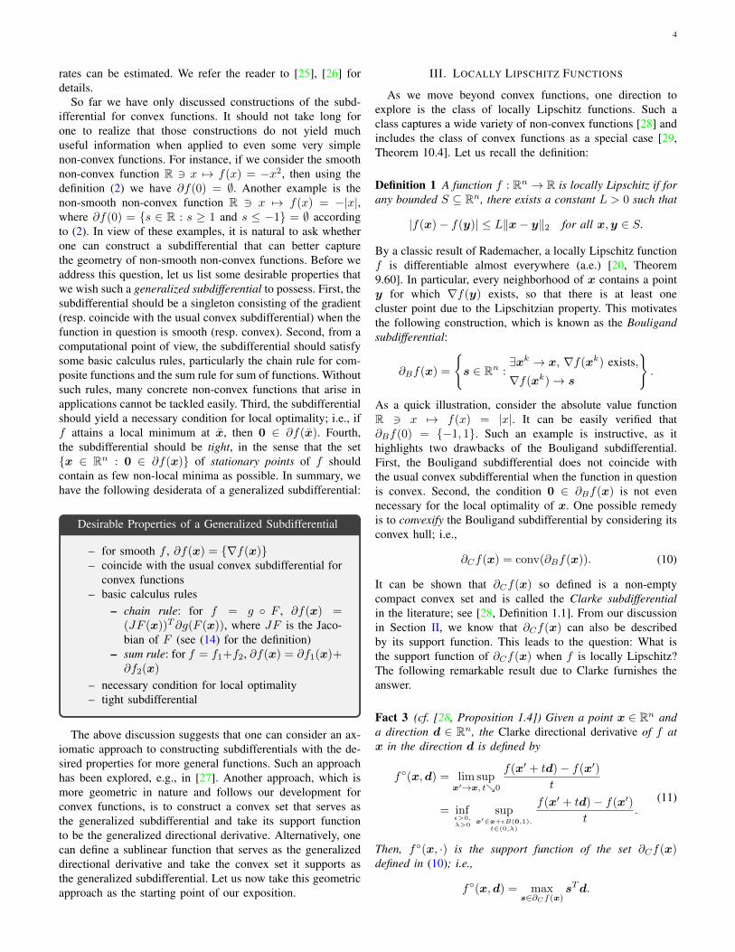
So far we have only discussed constructions of the subd-ifferential for convex functions. It should not take long forone to realize that those constructions do not yield muchuseful information when applied to even some very simplenon-convex functions. For instance, if we consider the smoothnon-convex function R 3 x 7→ f(x) = −x2, then using thedefinition (2) we have ∂f(0) = ∅. Another example is thenon-smooth non-convex function R 3 x 7→ f(x) = −|x|,where ∂f(0) = {s ∈ R : s ≥ 1 and s ≤ −1} = ∅ accordingto (2). In view of these examples, it is natural to ask whetherone can construct a subdifferential that can better capturethe geometry of non-smooth non-convex functions. Before weaddress this question, let us list some desirable properties thatwe wish such a generalized subdifferential to possess. First, thesubdifferential should be a singleton consisting of the gradient(resp. coincide with the usual convex subdifferential) when thefunction in question is smooth (resp. convex). Second, from acomputational point of view, the subdifferential should satisfysome basic calculus rules, particularly the chain rule for com-posite functions and the sum rule for sum of functions. Withoutsuch rules, many concrete non-convex functions that arise inapplications cannot be tackled easily. Third, the subdifferentialshould yield a necessary condition for local optimality; i.e., iff attains a local minimum at x, then 0 ∈ ∂f(x). Fourth,the subdifferential should be tight, in the sense that the set{x ∈ Rn : 0 ∈ ∂f(x)} of stationary points of f shouldcontain as few non-local minima as possible. In summary, wehave the following desiderata of a generalized subdifferential:

Desirable Properties of a Generalized Subdifferential

– for smooth f , ∂f(x) = {∇f(x)}– coincide with the usual convex subdifferential for

convex functions– basic calculus rules

– chain rule: for f = g ◦ F , ∂f(x) =(JF (x))T∂g(F (x)), where JF is the Jaco-bian of F (see (14) for the definition)

– sum rule: for f = f1+f2, ∂f(x) = ∂f1(x)+∂f2(x)

– necessary condition for local optimality– tight subdifferential

The above discussion suggests that one can consider an ax-iomatic approach to constructing subdifferentials with the de-sired properties for more general functions. Such an approachhas been explored, e.g., in [27]. Another approach, which ismore geometric in nature and follows our development forconvex functions, is to construct a convex set that serves asthe generalized subdifferential and take its support functionto be the generalized directional derivative. Alternatively, onecan define a sublinear function that serves as the generalizeddirectional derivative and take the convex set it supports asthe generalized subdifferential. Let us now take this geometricapproach as the starting point of our exposition.

III. LOCALLY LIPSCHITZ FUNCTIONS

As we move beyond convex functions, one direction toexplore is the class of locally Lipschitz functions. Such aclass captures a wide variety of non-convex functions [28] andincludes the class of convex functions as a special case [29,Theorem 10.4]. Let us recall the definition:

Definition 1 A function f : Rn → R is locally Lipschitz if forany bounded S ⊆ Rn, there exists a constant L > 0 such that

|f(x)− f(y)| ≤ L‖x− y‖2 for all x,y ∈ S.

By a classic result of Rademacher, a locally Lipschitz functionf is differentiable almost everywhere (a.e.) [20, Theorem9.60]. In particular, every neighborhood of x contains a pointy for which ∇f(y) exists, so that there is at least onecluster point due to the Lipschitzian property. This motivatesthe following construction, which is known as the Bouligandsubdifferential:

∂Bf(x) =

{s ∈ Rn :

∃xk → x, ∇f(xk) exists,

∇f(xk)→ s

}.

As a quick illustration, consider the absolute value functionR 3 x 7→ f(x) = |x|. It can be easily verified that∂Bf(0) = {−1, 1}. Such an example is instructive, as ithighlights two drawbacks of the Bouligand subdifferential.First, the Bouligand subdifferential does not coincide withthe usual convex subdifferential when the function in questionis convex. Second, the condition 0 ∈ ∂Bf(x) is not evennecessary for the local optimality of x. One possible remedyis to convexify the Bouligand subdifferential by considering itsconvex hull; i.e.,

∂Cf(x) = conv(∂Bf(x)). (10)

It can be shown that ∂Cf(x) so defined is a non-emptycompact convex set and is called the Clarke subdifferentialin the literature; see [28, Definition 1.1]. From our discussionin Section II, we know that ∂Cf(x) can also be describedby its support function. This leads to the question: What isthe support function of ∂Cf(x) when f is locally Lipschitz?The following remarkable result due to Clarke furnishes theanswer.

Fact 3 (cf. [28, Proposition 1.4]) Given a point x ∈ Rn anda direction d ∈ Rn, the Clarke directional derivative of f atx in the direction d is defined by

f◦(x,d) = lim supx′→x, t↘0

f(x′ + td)− f(x′)

t

= infε>0,λ>0

supx′∈x+εB(0,1),

t∈(0,λ)

f(x′ + td)− f(x′)

t.

(11)

Then, f◦(x, ·) is the support function of the set ∂Cf(x)defined in (10); i.e.,

f◦(x,d) = maxs∈∂Cf(x)

sTd.

5

In particular, we have

∂Cf(x) ={s ∈ Rn : sTd ≤ f◦(x,d) for all d ∈ Rn

},

(12)and the function d 7→ f◦(x,d) is finite sublinear for allx ∈ Rn. Additionally, we have f ′(x,d) ≤ f◦(x,d) if thedirectional derivative of f exists.

We remark that a locally Lipschitz function may not bedirectionally differentiable. In other words, the differencequotient in (3) may not have a limit even though it is boundeddue to the Lipschitzian property. Here, we give an example toshowcase such possibility.

Consider the function

R 3 x 7→ f(x) =

{x sin(log( 1

x )) if x > 0,0 otherwise.

It is clear that f is smooth on R \ {0}. Its derivativeat any x > 0 is given by f ′(x) = sin(log( 1

x )) −cos(log( 1

x )), which is bounded by 2. Using this andthe structure of f , it can be shown that f is locallyLipschitz. However, the directional derivative of f atx = 0 does not exist. In fact, the difference quotientq(t) = f(t)

t = sin(log( 1t )) does not converge, as can

be seen by considering the sequence tn = e−(n+12 )π

and computing

q(tn) = sin

((n+

1

2

)π

)=

{1 if n is even,−1 otherwise.

It is instructive to compare the two notions of directionalderivatives in (4) and (11) from a geometric point of view. Theformer considers the variation of f along a ray emanating fromx in the direction d (i.e., f(x+ tkd) vs. f(x) with tk ↘ 0),while the latter considers the variation of f in the directiond for points in the neighborhood of x (i.e., f(xk + tkd) vs.f(xk) with tk ↘ 0 and xk → x). In particular, the latter isable to explore the behavior of f in a neighborhood of x ratherthan just along a ray emanating from x. Generally, f◦(x,d) isan upper bound on the difference quotient in the neighborhoodof x. As we shall see, such an idea turns out to be very fruitfulwhen studying the local behavior of non-smooth functions.

Our discussion above reveals a fundamental difference inthe theory of subdifferentiation for convex functions and non-convex functions. Specifically, in the convex case, subdifferen-tiation entails linearization of the function at hand; in the non-convex case, subdifferentiation can be seen as a convexificationprocess. This allows the use of concepts from convex analysisto study the subdifferentials of non-convex functions.

Recall that in Section II, we have introudced several proper-ties that the generalized subdifferential should possess. Now,let us check whether the Clarke subdifferential possesses thoseproperties.

– (Smooth function). If f is smooth (i.e., continuouslydifferentiable) at x, then f◦(x,d) = ∇f(x)Td for alld ∈ Rn and ∂Cf(x) = {∇f(x)}; see [28, Proposition1.13].

– (Convex function). As mentioned above, convex func-tions are locally Lipschitz. In this case, the Clarkesubdifferential and Clarke directional derivative take onparticularly simple forms. Indeed, the Clarke subdiffer-ential coincides with the usual convex subdifferential (2)due to [29, Theorems 17.2 and 25.6]. In addition, thedirectional derivative of a convex function, which alwaysexists, is equal to the Clarke directional derivative; i.e.,

f◦(x,d) = f ′(x,d). (13)

– (Sum rule). The following example demonstrates thatthe sum rule ∂C(f1 + f2) = ∂Cf1 + ∂Cf2 does not holdin general. Consider the function f : R → R given byf(x) = max{x, 0}+min{0, x}. Let us compute ∂Cf1(0),∂Cf2(0), and ∂Cf(0):

f(x) =f1(x)+f2(x)

∂Cf(0) = {1}

f2(x) = min{x,0}

∂Cf2(0) = [0,1]∂Cf1(0) = [0,1]

f1(x) = max{x,0}

Observe that

∂Cf(0) = {1} ( ∂Cf1(0) + ∂Cf2(0) = [0, 2].

The failure of the sum rule is one of the obstacles tocomputing the Clarke subgradient. Nevertheless, not allis lost, as we still have the following weaker version ofthe sum rule:

∂C(f1 + f2) ⊆ ∂Cf1 + ∂Cf2;

see [28, Proposition 1.12].– (Tightness). It is known that if f attains a local minimum

at x, then 0 ∈ ∂Cf(x); see [30, Proposition 2.3.2]. ByFact 3, this is equivalent to f◦(x,d) ≥ 0 for all d ∈ Rn.However, the Clarke subdifferential may contain sta-tionary points that are not local minima. For instance,consider the function R 3 x 7→ f(x) = −|x|. It is easyto see that ∂Cf(0) = [−1, 1]. It follows that x = 0 isa stationary point (as 0 ∈ ∂Cf(0)). However, the pointx = 0 is clearly not a local minimum (in fact, it is a globalmaximum). Moreover, observe that the correspondingClarke directional derivatives are f◦(0, 1) = f◦(0,−1) =1, which shows that neither d = 1 nor d = −1is a descent direction according to Clarke’s definition.However, the ordinary directional derivatives exist andare given by f ′(0, 1) = f ′(0,−1) = −1. It follows thatboth d = 1 and d = −1 are descent directions. One mayargue that the above example is not persuasive enough,as similar phenomena occur in the smooth case (e.g.,R 3 x 7→ f(x) = −x2). Hence, let us provide another,perhaps more convincing, example:

6

Consider the function

R 3 x 7→ f(x) =

{x+ x2 sin( 1

x ) if x > 0,x otherwise.

x

f(x)

-1 0 1

1

For x > 0, f ′(x) = 1 + 2x sin( 1x ) − cos( 1

x )is bounded on compact sets. Using this and thestructure of f , it can be shown that f is locallyLipschitz. On one hand, we have ∂Cf(0) = [0, 2],which means that x = 0 is a stationary point. Onthe other hand, we have f ′(0, 1) = f ′(0,−1) = 1.Hence, the point x = 0 is neither a local minimumnor a local maximum.

Observe that in the above examples, the ordinary di-rectional derivative exists but is strictly smaller thanthe corresponding Clarke directional derivatives (i.e.,f ′(x,d) < f◦(x,d)). This, together with (12), suggeststhat one may obtain a tighter subdifferential by usingother directional derivatives.

In view of the aforementioned drawbacks of the Clarkesubdifferential, it is natural to ask whether the notion is usefulin applications. As it turns out, the Clarke subdifferential canstill be a very powerful tool for studying certain sub-classesof locally Lipschitz functions.

IV. SUBDIFFERENTIALLY REGULAR FUNCTIONS

In this section, we introduce a representative function classcalled subdifferentially regular functions. The Clarke subdif-ferential for such functions preserves many of the nice prop-erties of the subdifferential for convex functions. This greatlyfacilitates the manipulation of such functions in computationalprocedures.

Definition 2 ([30, Definition 2.3.4]) A locally Lipschitz func-tion f : Rn → R is subdifferentially regular (or simply regular)at x ∈ Rn if for every d ∈ Rn, the ordinary directionalderivative (4) exists and coincides with the generalized one in(11):

f ′(x,d) = f◦(x,d).

If f is regular at every x ∈ Rn, then we simply say that f isregular.

As a first example, we note that a convex function f is regular.This follows immediately from (13). In this case, we have∂Cf = ∂f . Another important example of a regular functionis the max function given by f = maxi∈{1,...,m} gi, where gi :Rn → R (i = 1, . . . ,m) is smooth; see [20, Example 7.28].

In particular, this implies that a smooth function is regular.Upon letting I(x) = {i ∈ {1, . . . ,m} : f(x) = gi(x)} bethe set of indices whose corresponding functions gi is activeat x, we have ∂Cf(x) = conv{∇gi(x) : i ∈ I(x)}; see [20,Exercise 8.31]. We remark that a similar result holds for maxfunctions involving an infinite collection of smooth functions.The interested reader is referred to [20, Theorem 10.31] fordetails.

One of the nice properties of regular functions is that theysatisfy the following basic calculus rules.

Fact 4 (cf. [20, Theorem 10.6, Corollary 10.9])(a) (Chain Rule). Suppose that f : Rn → R takes the form

f = g ◦ F , where g : Rm → R is a locally Lipschitzfunction and F : Rn → Rm is a smooth mapping. Givena point x ∈ Rn, if g is regular at F (x), then f is regularat x and

∂Cf(x) = (JF (x))T∂Cg(F (x)),

where JF is the Jacobian of F ; i.e.,

JF (x) =

[∂fi∂xj

(x)

]m,ni,j=1

∈ Rm×n. (14)

In particular, for a real-valued function F : Rn → R,the gradient of F at x is given by ∇F (x) = (JF (x))T .

(b) (Sum Rule). Suppose that f = f1 + f2 + · · · + fm,where fi : Rn → R (i = 1, . . . ,m) are locally Lipschitzfunctions. Given a point x ∈ Rn, if f1, . . . , fm areregular at x, then so is f and

∂Cf(x) = ∂Cf1(x) + ∂Cf2(x) + · · ·+ ∂Cfm(x).

We remark that it is possible to develop (possibly weaker)versions of the above calculus rules under weaker assumptions.For instance, a variant of the above chain rule holds in thesetting where g is lower semi-continuous1 and F is a locallyLipschitz mapping (and thus not necessarily smooth), whilea variant of the above sum rule holds in the setting wheref1, . . . , fm are lower semi-continuous. We refer the readerto [20, Theorems 10.6 and 10.49] for details.

To illustrate the usefulness of the above calculus rules, letus turn our attention to another fundamental class of regularfunctions, namely weakly convex functions. Such functionshave recently received much attention, as they arise in manycontemporary signal processing and machine learning appli-cations. We begin with the definition.

Definition 3 A function f : Rn → R is called ρ-weaklyconvex (with ρ ≥ 0) if the function x 7→ h(x) = f(x)+ ρ

2‖x‖22

is convex.

It is immediate from the definition that a convex function is0-weakly convex. As it turns out, weakly convex functionsare locally Lipschitz and regular; see [31, Propositions 4.4and 4.5]. This implies that the basic calculus rules in Fact 4

1Recall that a function f : Rn → R is lower semi-continuous iflim infy→x f(y) = f(x), or equivalently, the epigraph epi(f) = {(x, t) ∈Rn × R : f(x) ≤ t} of f is closed in Rn × R; see [20, Theorem 1.6].

7

can be applied to weakly convex functions. In particular, wecan compute the subdifferential of a weakly convex functionf as follows. By definition, the function Rn 3 x 7→ h(x) =f(x) + ρ

2‖x‖22 is convex for some ρ ≥ 0. Using the fact that

x 7→ ρ2‖x‖

22 is regular and applying the sum rule, we have

∂Ch(x) = ∂Cf(x)+{ρx}. Since ∂Ch equals the usual convexsubdifferential ∂h of h, we obtain

∂Cf(x) = ∂h(x)− {ρx}.

Weakly convex functions are ubiquitous in applications. Oneprototypical example is the composite function f = g ◦ F ,where g : Rm → R is convex and Lipschitz continuous onRm and F : Rn → Rm is a smooth map with Lipschitzcontinuous Jacobian [32]. Note that the chain rule in Fact 4yields a formula for ∂Cf . Below are some concrete examplesof such a composite function that arise in applications.

– (Robust low-rank matrix recovery). In various signalprocessing [33] and machine learning [34] applications,a fundamental computational task is to recover a low-rank matrix X? ∈ Rn1×n2 from a small number of noisylinear measurements of the form

y = A(X?) + s?,

where A : Rn1×n2 → Rm is a known linear operator,s? ∈ Rm is a noise vector, and y ∈ Rm is the vectorof observed values. For simplicity, let us assume that theground-truth matrix X? is an n × n symmetric positivesemidefinite matrix of rank r ≥ 1. In the setting wherethe noise vector represents outliers in the measurements,the `1-loss function is usually preferred over the `2-lossfor recovering the ground-truth signal. This gives rise tothe following weakly convex formulation for recoveringX? [5]:

minU∈Rn×r

f(U) =1

m

∥∥y −A(UUT )∥∥1.

By applying the chain rule in Fact 4, we can compute

1

m

[(A∗(Sign(A(UUT )− y)))TU

+A∗(Sign(A(UUT )− y))U]⊆ ∂Cf(U),

where A∗ is the adjoint of A; see [5].– (Robust sign retrieval). Phase retrieval is a classic

inverse problem that arises in areas such as crystallog-raphy [19], optical imaging [35], and audio signal pro-cessing [36]. Here, let us consider a real-valued versionof the problem, in which we are interested in recoveringa vector x? ∈ Rn from noisy measurements of the form

bi = (aTi x?)2 + s?i for i = 1, . . . ,m, (15)

where a1, . . . ,am ∈ Rn are measurement vectors, s? ∈Rm is the noise vector, and b1, . . . , bm ∈ R are theobserved values. One approach to tackling this problemis to consider the weakly convex formulation

minx∈Rn

f(x) =1

m

m∑i=1

∣∣(aTi x)2 − bi∣∣ ,

which aims at handling outliers in the measurements [37],[38]. Using the calculus rules in Fact 4, we have

2

m

m∑i=1

(aTi x) · Sign((aTi x)2 − bi) · ai ⊆ ∂Cf(x);

see [38].– (Robust blind deconvolution). The blind deconvolution

problem, which is found in diverse fields such as astron-omy [39] and image processing [40], [41], aims to recovera pair of signals in two low-dimensional structured spacesfrom observations of their noisy pairwise convolutions.Again, let us focus on a real-valued version of thisproblem for simplicity. Formally, we consider the task ofrobustly recovering a pair (w?,x?) ∈ Rn1 × Rn2 fromm bilinear measurements:

bi = (aTi w?)(cTi x

?) + s?i for i = 1, . . . ,m,

where a1, . . . ,am ∈ Rn1 and c1, . . . , cm ∈ Rn2 aremeasurement vectors, b1, . . . , bm ∈ R are the observedvalues, and s? ∈ Rm is the noise vector. One non-smoothformulation of the problem reads

minw∈Rn1 ,x∈Rn2

f(w,x) =1

m

m∑i=1

∣∣(aTi w)(cTi x)− bi∣∣ ,

in which the `1-loss promotes strong recovery and stabil-ity guarantees under certain statistical assumptions [42].By invoking the chain rule in Fact 4, we obtain

1

m

m∑i=1

Sign((aTi w)(cTi x)− bi)·((cTi x)

[ai0

]+ (aTi w)

[0ci

])⊆ ∂Cf(w,x);

see [42].Another illustrative example is given by the family of

weakly convex sparse regularizers [43], [44], such as loga-rithmic sum penalty [45], smoothly clipped absolute deviation(SCAD) [46], and minimax concave penalty (MCP) [47].These regularizers take the form

Rn 3 x 7→ R(x) =

n∑i=1

φ(|xi|),

where φ : R → R is a non-decreasing concave but weaklyconvex function. Although we cannot apply the chain rulein Fact 4 directly, by using the fact that the absolute valuefunction is locally Lipschitz, we can still apply an extendedversion of the chain rule (see [20, Theorem 10.49]) to computean element of the subdifferential of R. Let us demonstrate thisvia the following concrete example:

Let R : Rn → R be the logarithmic sum penaltyfunction; i.e.,

R(x) =

d∑i=1

log (|xi|+ θ) ,

where θ > 0 is a smoothing parameter. Consider the

8

following regularized least-squares regression prob-lem:

minx∈Rn

f(x) =1

2m

m∑i=1

(bi − a>i x

)2+ λR(x),

where λ ≥ 0 is a regularization parameter. Observethat f is regular, as the sum of regular functions isregular; see Fact 4. By the extended chain rule, anyvector s ∈ Rn with

si ∈Sign(xi)

|xi|+ θfor i = 1, . . . , n

satisfies s ∈ ∂CR(x). It is then straightforward toobtain an element of the subdifferential of f via thesum rule in Fact 4.

In all the above examples, the ability to explicitly calculatethe subdifferential of the weakly convex objective functionat hand makes it possible to use simple subgradient methodsto minimize the function. Moreover, if the objective functionsatisfies a regularity condition called sharpness, then a suitablyinitialized subgradient method with properly chosen step sizeswill converge at a linear rate to an optimal solution to the prob-lem [32] (see also [5], [38]). We also refer the reader to [48],which discusses stochastic methods for tackling optimizationproblems involving weakly convex objective functions, andto [49], which develops Riemannian subgradient-type methodsfor weakly convex optimization over the Stiefel manifold.

Although the class of weakly convex functions provides apowerful modeling tool for applications in signal processingand machine learning, there are still other widely-used func-tions that do not belong to this class. Here are two examples.

– (Canonical robust sign retrieval). Besides the squared-amplitude measurement model in (15), another measure-ment model of interest for phase retrieval problems is

bi = |aTi x?|+ s?i for i = 1, . . . ,m,

where x? ∈ Rn is the signal to be recovered,a1, . . . ,am ∈ Rn are measurement vectors, s? ∈ Rmis the noise vector, and b1, . . . , bm ∈ R are the observedvalues. Such an amplitude measurement model is used,e.g., in optical wavefront reconstruction; see [50] fordetails. The corresponding robust phase retrieval problemthen takes the form

minx∈Rn

f(x) =1

m

m∑i=1

∣∣|aTi x| − bi∣∣ .The function f is not weakly convex as it is not evensubdifferentially regular [51].

– (Deep Neural Network). Deep learning is a powerfulparadigm in machine learning that allows one to learna complicated mapping by decomposing it into a seriesof nested simple mappings, and it has attracted immenseinterest in various areas of science and engineering [52].As an illustration, consider a simple prediction problem,in which one is given N observed feature-label pairs(xi, yi) ∈ Rn×R, where i = 1, . . . , N , and the goal is to

learn the feature-label relationship. One can model sucha relationship using the one-hidden-layer neural networkshown in Figure 3. Here, W = [w1, . . . ,wk] is the

Fig. 3. Illustration of one-hidden-layer neural network.

matrix of weight parameters, where wj ∈ Rn denotes theweight with respect to the j-th neuron, and σ : R → Ris a (typically non-smooth) activation function (e.g., theReLU function x 7→ max{x, 0}). Using the square-lossfunction, the weights that best model the relationship inthe given feature-label pairs can be found by solving thefollowing optimization problem:

minW∈Rn×k

f(W ) =1

2N

N∑i=1

k∑j=1

σ(wTj xi)− yi

2

.

(16)Unfortunately, neural networks with non-smooth activa-tion functions typically give rise to objective functionsthat are not subdifferentially regular [53]. For example,consider the instance of Problem (16) in which N =n = k = 1, x1 = y1 = 1, and σ : R → R is the ReLUfunction (i.e., σ(x) = max{x, 0}). Then, the objectivefunction in (16) becomes f(w) = 1

2 (max{w, 0} − 1)2,whose graph is shown below.

w

f(w)

-1 1

1/2

It is a simple exercise to show that f◦(0, 1) >0 > f ′(0, 1). Hence, by Definition 2, we see that fis not subdifferentially regular. Roughly speaking, thegraph of a subdifferentially regular function cannot have“downward-facing cusps” [53].

In view of the above examples, we are naturally interested indeveloping other sharper generalized subdifferential conceptsthat can deal with broader function classes.

V. DIRECTIONALLY DIFFERENTIABLE FUNCTIONS

As we have seen in Section III, the Clarke directionalderivative f◦ does not always yield useful information aboutthe descent directions of a function at a given point. For

9

instance, for a directionally differentiable locally Lipschitzfunction f with directional derivative f ′, we always havef ′ ≤ f◦ and hence the Clarke subdifferential is in somesense too large; see Fact 3. We circumvent this problem inSection IV by imposing the assumption f ′ = f◦ on thefunctions we consider, thereby leading us to the class ofsubdifferentially regular functions. In this section, we presentanother approach, which begins by constructing subdifferen-tials that are smaller than the Clarke subdifferential and thentrying to refine them so that they possess some of the desirableproperties mentioned in Section II. One advantage of such anapproach is that it allows us to tackle functions that are notnecessarily subdifferentially regular.

To begin, consider a directionally differentiable locallyLipschitz function f : Rn → R; i.e., the directional derivativef ′(x,d) exists for all x ∈ Rn and d ∈ Rn. Since f ′ ≤ f◦ byFact 3, the following set suggests itself as a natural candidatefor a subdifferential of f :

∂f(x) ={s ∈ Rn : sTd ≤ f ′(x,d) for all d ∈ Rn

}. (17)

The set ∂f(x) is known as the Frechet subdifferential and itselements the Frechet subgradients of f at x. It is immediatefrom (17) that ∂f(x) ⊆ ∂Cf(x) for any x ∈ Rn (see (12)),and that the Frechet subdifferential coincides with the usualconvex subdifferential when f is convex (see (5)). In fact,the Frechet subdifferential is closely related to the convexsubdifferential. Specifically, the former can be obtained byusing higher-order minorants in the construction (2) of theconvex subdifferential (see [20, Exercises 8.4 and 9.15]):

∂f(x) =

{s ∈ Rn :

f(y) ≥ f(x) + sT (y − x)

+ o(‖y − x‖2) for all y ∈ Rn

}.

The inequality with the little-oh term in the above expressionmeans that

lim infy→x

f(y)− f(x)− sT (y − x)

‖y − x‖2≥ 0.

Moreover, observe that for any x ∈ Rn, we have f ′(x, td) =t·f ′(x,d) for any d ∈ Rn and t > 0. Hence, by [20, Theorem8.24], the set ∂f(x) is closed and convex. In addition, sincef ′(x,d) <∞ for all d ∈ Rn due to the Lipschitzian propertyof f , the support function of ∂f(x) is given by conv(f ′(x, ·));i.e.,

conv(f ′(x, ·))(d) = sups∈∂f(x)

sTd,

where conv(f ′(x, ·)) is the pointwise supremum of all convexfunctions g satisfying g(d) ≤ f ′(x,d) for all d ∈ Rn. Werefer the interested reader to [54], [55] for a detailed treatmentof the Frechet subdifferential.

Although the above discussion suggests that the Frechetsubdifferential possesses many attractive properties, it is stillrather limited. Consider, for instance, the directionally differ-entiable Lipschitz function R 3 x 7→ f(x) = −|x|. Then, asimple calculation yields ∂f(0) = ∅. In particular, the Frechetsubdifferential can be empty, even at points that could be ofinterest (in this case, x = 0 is the global maximum). Moreover,by taking a sequence xk ↘ 0, we have −1 ∈ ∂f(xk) for all

k but −1 6∈ ∂f(0); i.e., the mapping ∂f is not closed. Thisshows that the Frechet subdifferential is not stable with respectto small perturbations of the point in question, which can causeinstabilites in computation. One way of addressing this issue isto “close” the mapping ∂f by defining the following limitingsubdifferential of f :

∂f(x) =

{s ∈ Rn :

∃xk → x and sk ∈ ∂f(xk)

such that sk → s

}. (18)

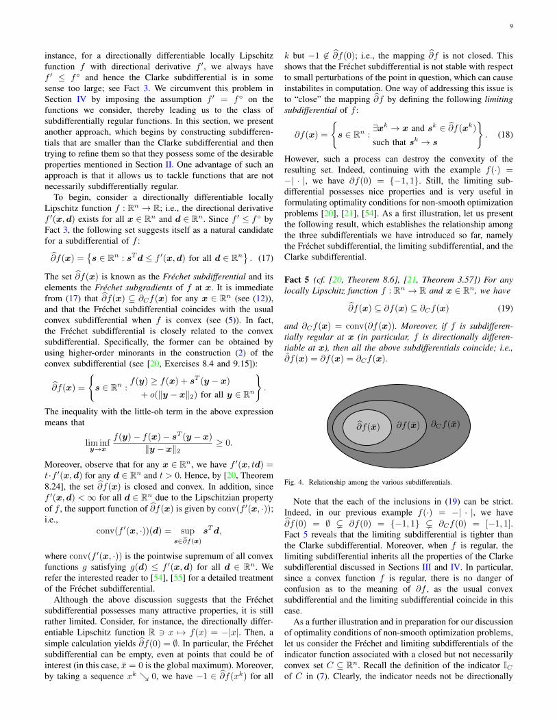
However, such a process can destroy the convexity of theresulting set. Indeed, continuing with the example f(·) =−| · |, we have ∂f(0) = {−1, 1}. Still, the limiting sub-differential possesses nice properties and is very useful informulating optimality conditions for non-smooth optimizationproblems [20], [21], [54]. As a first illustration, let us presentthe following result, which establishes the relationship amongthe three subdifferentials we have introduced so far, namelythe Frechet subdifferential, the limiting subdifferential, and theClarke subdifferential.

Fact 5 (cf. [20, Theorem 8.6], [21, Theorem 3.57]) For anylocally Lipschitz function f : Rn → R and x ∈ Rn, we have

∂f(x) ⊆ ∂f(x) ⊆ ∂Cf(x) (19)

and ∂Cf(x) = conv(∂f(x)). Moreover, if f is subdifferen-tially regular at x (in particular, f is directionally differen-tiable at x), then all the above subdifferentials coincide; i.e.,∂f(x) = ∂f(x) = ∂Cf(x).

∂f(x) ∂f(x) ∂Cf(x)

Fig. 4. Relationship among the various subdifferentials.

Note that the each of the inclusions in (19) can be strict.Indeed, in our previous example f(·) = −| · |, we have∂f(0) = ∅ ( ∂f(0) = {−1, 1} ( ∂Cf(0) = [−1, 1].Fact 5 reveals that the limiting subdifferential is tighter thanthe Clarke subdifferential. Moreover, when f is regular, thelimiting subdifferential inherits all the properties of the Clarkesubdifferential discussed in Sections III and IV. In particular,since a convex function f is regular, there is no danger ofconfusion as to the meaning of ∂f , as the usual convexsubdifferential and the limiting subdifferential coincide in thiscase.

As a further illustration and in preparation for our discussionof optimality conditions of non-smooth optimization problems,let us consider the Frechet and limiting subdifferentials of theindicator function associated with a closed but not necessarilyconvex set C ⊆ Rn. Recall the definition of the indicator ICof C in (7). Clearly, the indicator needs not be directionally

10

differentiable or locally Lipschitz. Nevertheless, a formalcalculation using the definition of the Frechet subdifferentialin (17) yields

∂IC(x) =

{s ∈ Rn :

sT (y − x) ≤ o(‖y − x‖2)

for all y ∈ C

}(20)

if x ∈ C and ∂IC(x) = ∅ otherwise. The defining conditionof the set on the right-hand side of (20) can also be written as

lim supy→x,y∈C

sT (y − x)

‖y − x‖2≤ 0.

The formula (20) for ∂IC(x) is indeed valid and can beestablished in a rigorous manner [20, Exercise 8.14]. The seton the right-hand side of (20) is called the Frechet normalcone to C at x and is denoted by NC(x); cf. the discussionfollowing (8). Now, using (18) and (20), we can compute thelimiting subdifferential of IC as

∂IC(x) =

{s ∈ Rn :

∃xk → x and sk ∈ NC(xk)

such that sk → s

}; (21)

see [20, Definition 6.3 and Exercise 8.14]. Following theterminology used above, the set on the right-hand side of (21)is called the limiting normal cone of C at x and is denoted byNC(x). Figures 5 and 6 show the Frechet and limiting normalcones of two closed non-convex sets. It is worth noting that thetwo normal cones do not always coincide; see Figure 6, whereNC(x) consists of the zero vector only and NC(x) consistsof the two rays emanating from x. In general, we always haveNC(x) ⊆ NC(x) [20, Proposition 6.5].

Cx

NC(x) = NC(x)

Fig. 5. A closed non-convex set with NC(x) = NC(x).

NC (x)

NC (x) = {0}

C

x

Fig. 6. A closed non-convex set with NC(x) ( NC(x).

A. Concepts of Stationarity

Armed with the above development, we are now ready toaddress our primary goal of this paper, which is to introduce

and compare different stationarity concepts for non-convexnon-smooth optimization problems. To begin, consider Prob-lem (9), where g : Rn → R is a directionally differentiablelocally Lipschitz function and C ⊆ Rn is a closed set. Wesay that x ∈ Rn is a directional stationary (resp. limitingstationary and Clarke stationary) point of Problem (9) if 0 ∈∂(g+IC)(x) (resp. 0 ∈ ∂(g+IC)(x) and 0 ∈ ∂C(g+IC)(x)).The following result gives a necessary condition for localoptimality of a feasible solution to Problem (9):

Fact 6 (cf. [20, Theorems 8.15 and 10.1, Corollary 6.29]) Ifx is a local minimum of (9), then x is a directional stationary(d-stationary) point of (9). If in addition g and IC are regularat x, then

f ′(x,d) ≥ 0 for all d ∈ N ◦C(x),

where

N ◦C(x) ={d ∈ Rn : sTd ≤ 0 for all s ∈ NC(x)

}is called the polar of NC(x).

Note that if x is a d-stationary point of (9), then by Facts 5and 6 it is also a limiting stationary (l-stationary) and Clarkestationary (C-stationary) point of (9). In particular, we havethe following implications:

d-stationarity =⇒ l-stationarity =⇒ C-stationarity.

We now give two examples to show that the reverse implica-tions need not hold in general; see [9].

−10

f2(x) = max{−x−1,min{−x,0}}

0

0.5

f1(x) = max{−|x|,x−1}

– For the univariate function f1 : R → R, wehave ∂Cf1(0) = [−1, 1] and ∂f1(0) = {−1, 1}.It follows that the point x = 0 is C-stationarybut fails to be l-stationary. The unique l-stationarypoint is x? = 0.5 and is also a local minimum.

– For the univariate function f2 : R→ R, we have∂f2(0) = {−1, 0} and ∂f2(0) = ∅. It follows thatthe point x = 0 is l-stationary but not d-stationary.The unique d-stationary point is x? = −1 and isalso a local minimum.

The above discussion suggests that among the three notionsof stationarity, d-stationarity is the sharpest. However, thedevelopment of algorithms for computing a d-stationary pointof the non-convex non-smooth optimization problem (9) isstill in the infancy stage. We will briefly discuss a recenteffort in this direction in the next sub-section and refer thereader to [9], [56] for further reading. By contrast, underthe assumption that g + IC satisfies the so-called Kurdyka-Łojasiewicz property, various algorithms will produce iterates

11

that are provably convergent to a limiting stationary pointof (9); see, e.g., [57].

B. Application: Least Squares Piecewise Affine Regression

In this sub-section, we discuss a representative applicationcalled Least Squares Piecewise Affine Regression, in whichthe objective function is piecewise linear-quadratic (PLQ) andhence directionally differentiable (see [20, Proposition 10.21]).Specifically, the objective function takes the form

minW∈C

f(W ) =1

2N

N∑s=1

(ys − max

1≤i≤kwTi xs

)2

, (22)

where W = [w1, . . . ,wk] ∈ Rn×k is the matrix of decisionvariables and C ⊆ Rn×k is the feasible set. By setting hs(u) =(ys−u)2 (the square loss) and gs(W ) = max1≤i≤kw

Ti xs (a

piecewise affine function), we can write the above problem inthe following compact form:

minW∈C

f(W ) =1

2N

N∑s=1

hs(gs(θ)).

The above problem can be used to model the one-layerneural network with the ReLU activation function, in whichk = 1, C = Rn, and gs takes the simple form gs(w) =max{wTxs, 0}; cf. (16). Our interest in Problem (22) stemsfrom the following:

Fact 7 (cf. [58, Proposition 16]) The least squares piecewiseaffine regression problem (22) possesses the following proper-ties:

(a) It attains a finite global minimum value.(b) The set of d-stationary points is finite.(c) Every d-stationary point is a local minimizer.

The above result provides further evidence that the notion of d-stationarity is in some sense the sharpest, as every d-stationarypoint of Problem (22) is a local minimum. In view of this, it isnatural to ask whether we can propose an iterative algorithm tofind such points. In [9] the authors proposed a non-monotonemajorized-minimization (MM) algorithm with a semi-smoothNewton method as its inner solver to find a d-stationary pointof a class of so-called composite difference-convex-piecewiseoptimization problems, of which Problem (22) is an instance.They also showed that the MM algorithm will converge toa d-stationary point of such problems under mild conditions(which are satisfied by (22)). One of the motivations forintroducing such an algorithm is that it is not known whetherthe basic chain rule holds for the objective function in (22).For the purpose of experimentation, let us pretend the basicchain rule holds and use it to compute a pseudo-subgradient(actually back-propagation in deep learning) of the objectivefunction:

∂f(wi)

∂wi=

1

2

N∑s=1

(max1≤i≤k

wTi xs − ys

)xsI{

i∈argmaxi

wTi xs

}.Then, we can try using the subgradient method with such apseudo-subgradient to tackle Problem (22). However, such an

0 100 200 300 400 500

Repeating Experiments

0

0.01

0.02

0.03

0.04

0.05

0.06

0.07

0.08

Opt

imal

val

ues

for

diffe

rent

ial i

nitia

l poi

nts

Subgradient MethodMajorized-Minimization

Fig. 7. Objective values computed by the MM and subgradient algorithms,N = 10.

approach does not quite work empirically. Indeed, let us followthe experimental setup in [9] and consider the 2-dimensionalconvex piecewise linear model

y = max {x1 + x2, x1 − x2,−2x1 + x2,−2x1 − x2}+ ε

with different sample sizes N = 10, 50, 100. We test theMM and subgradient algorithms on synthetic data. Using thesame initial points for the two algorithms, all the experimentresults reported here were collected over 500 independenttrials over random seeds. From Figures 7 and 8, we observe

N = 10 N=50 N=1000

50

100

150

200

250

300

350

MMSubgradient

Fig. 8. Number of initial points that lead to the smallest objective values.

that there is an apparent gap between these two algorithms.In particular, the figures show that the subgradient algorithmreaches many limit points that are unsatisfactory. Nevertheless,the MM algorithm can be rather slow. As a future work, itwould be interesting to design practically efficient first-orderalgorithms that can provably return a d-stationary point for thisapplication, and more generally, for other signal processing,machine learning, and statistical applications; see, e.g., [8]–[10], [56], [58] and the references therein.

VI. CONCLUSION

In this article, we elucidated the constructions of vari-ous subdifferentials for several important sub-classes of non-

12

smooth functions and discussed their corresponding station-arity concepts. We also showcased several representative ex-amples and applications to illustrate the differences amongvarious constructions. We hope that this introductory articlewill serve as a good starting point for readers who would liketo utilize the mathematical tools from non-smooth analysis inthe design and analysis of iterative methods for non-smoothoptimization problems.

REFERENCES

[1] Y. Koren, R. Bell, and C. Volinsky, “Matrix Factorization Techniquesfor Recommender Systems,” Computer, vol. 42, no. 8, pp. 30–37, 2009.

[2] R. Ge, J. D. Lee, and T. Ma, “Matrix Completion has No SpuriousLocal Minima,” in Advances in Neural Information Processing Systems29: Proceedings of the 2016 Conference, D. D. Lee, M. Sugiyama, U. V.Luxburg, I. Guyon, and R. Garnett, Eds., 2016, pp. 2973–2981.

[3] S. Tu, R. Boczar, M. Simchowitz, M. Soltanolkotabi, and B. Recht,“Low–Rank Solutions of Linear Matrix Equations via Procrustes Flow,”in Proceedings of the 33rd International Conference on Machine Learn-ing (ICML 2016), 2016, pp. 964–973.

[4] Y. Li, Y. Chi, H. Zhang, and Y. Liang, “Nonconvex Low–Rank Ma-trix Recovery with Arbitrary Outliers via Median–Truncated GradientDescent,” Information and Inference: A Journal of the IMA, p. iaz009,2019.

[5] X. Li, Z. Zhu, A. M.-C. So, and R. Vidal, “Nonconvex Robust Low–Rank Matrix Recovery,” SIAM Journal on Optimization, vol. 30, no. 1,pp. 660–686, 2020.

[6] P.-L. Loh and M. J. Wainwright, “High–Dimensional Regression withNoisy and Missing Data: Provable Guarantees with Nonconvexity,” TheAnnals of Statistics, vol. 40, no. 3, pp. 1637–1664, 2012.

[7] ——, “Regularized M–Estimators with Nonconvexity: Statistical andAlgorithmic Theory for Local Optima,” Journal of Machine LearningResearch, vol. 16, no. Mar, pp. 559–616, 2015.

[8] M. Ahn, J.-S. Pang, and J. Xin, “Difference–of–Convex Learning:Directional Stationarity, Optimality, and Sparsity,” SIAM Journal onOptimization, vol. 27, no. 3, pp. 1637–1665, 2017.

[9] Y. Cui, J.-S. Pang, and B. Sen, “Composite Difference–Max Programsfor Modern Statistical Estimation Problems,” SIAM Journal on Opti-mization, vol. 28, no. 4, pp. 3344–3374, 2018.

[10] M. Nouiehed, J.-S. Pang, and M. Razaviyayn, “On the Pervasivenessof Difference–Convexity in Optimization and Statistics,” MathematicalProgramming, Series B, vol. 174, no. 1–2, pp. 195–222, 2019.

[11] A. Krizhevsky, I. Sutskever, and G. E. Hinton, “ImageNet Classificationwith Deep Convolutional Neural Networks,” in Advances in Neural In-formation Processing Systems 25: Proceedings of the 2012 Conference,P. Bartlett, F. C. N. Pereira, C. J. C. Burges, L. Bottou, and K. Q.Weinberger, Eds., 2012, pp. 1097–1105.

[12] D. P. Kingma and J. L. Ba, “Adam: A Method for Stochastic Optimiza-tion,” in Proceedings of the 3rd International Conference on LearningRepresentations (ICLR 2015), 2015.

[13] X. Chen, S. Liu, R. Sun, and M. Hong, “On the Convergence of A Classof Adam–Type Algorithms for Non–Convex Optimization,” in Proceed-ings of the 7th International Conference on Learning Representations(ICLR 2019), 2019.

[14] J. Sun, Q. Qu, and J. Wright, “Complete Dictionary Recovery Over theSphere I: Overview and the Geometric Picture,” IEEE Transactions onInformation Theory, vol. 63, no. 2, pp. 853–884, 2017.

[15] ——, “Complete Dictionary Recovery Over the Sphere II: Recovery byRiemannian Trust–Region Method,” IEEE Transactions on InformationTheory, vol. 63, no. 2, pp. 885–914, 2017.

[16] C.-J. Lin, “Projected Gradient Methods for Nonnegative Matrix Factor-ization,” Neural Computation, vol. 19, no. 10, pp. 2756–2779, 2007.

[17] Y. Li, Y. Liang, and A. Risteski, “Recovery Guarantee of Non–NegativeMatrix Factorization via Alternating Updates,” in Advances in Neural In-formation Processing Systems 29: Proceedings of the 2016 Conference,D. D. Lee, M. Sugiyama, U. V. Luxburg, I. Guyon, and R. Garnett, Eds.,2016, pp. 4987–4995.

[18] T. Bendory, Y. C. Eldar, and N. Boumal, “Non–Convex Phase Retrievalfrom STFT Measurements,” IEEE Transactions on Information Theory,vol. 64, no. 1, pp. 467–484, 2018.

[19] V. Elser, T.-Y. Lan, and T. Bendory, “Benchmark Problems for PhaseRetrieval,” SIAM Journal on Imaging Sciences, vol. 11, no. 4, pp. 2429–2455, 2018.

[20] R. T. Rockafellar and R. J.-B. Wets, Variational Analysis, 2nd ed., ser.Grundlehren der mathematischen Wissenschaften. Berlin Heidelberg:Springer–Verlag, 2004, vol. 317.

[21] B. S. Mordukhovich, Variational Analysis and Generalized Differenti-ation I: Basic Theory, 2nd ed., ser. Grundlehren der mathematischenWissenschaften. Berlin Heidelberg: Springer–Verlag, 2013, vol. 330.

[22] J.-B. Hiriart-Urruty and C. Lemarechal, Fundamentals of Convex Analy-sis, ser. Grundlehren Text Editions. Berlin/Heidelberg: Springer–Verlag,2001.

[23] P. Wolfe, “A method of conjugate subgradients for minimizing non-differentiable functions,” Mathematical Programming Study, vol. 3, pp.145–173, 1975.

[24] K. C. Kiwiel, Methods of Descent for Nondifferentiable Optimization,ser. Lecture Notes in Mathematics. Berlin Heidelberg: Springer–Verlag,1985, vol. 1133.

[25] J. L. Goffin, “On convergence rates of subgradient optimization meth-ods,” Mathematical Programming, vol. 13, no. 1, pp. 329–347, 1977.

[26] N. Z. Shor, Minimization Methods for Non–Differentiable Functions,ser. Springer Series in Computational Mathematics. Berlin Heidelberg:Springer–Verlag, 1985, vol. 3.

[27] A. D. Ioffe, “On the theory of subdifferentials,” Advances in NonlinearAnalysis, vol. 1, no. 1, pp. 47–120, 2012.

[28] F. H. Clarke, “Generalized Gradients and Applications,” Transactions ofthe American Mathematical Society, vol. 205, no. Apr., pp. 247–262,1975.

[29] R. T. Rockafellar, Convex Analysis, ser. Princeton Landmarks in Mathe-matics and Physics. Princeton, New Jersey: Princeton University Press,1997.

[30] F. H. Clarke, Optimization and Nonsmooth Analysis, ser. Classics in Ap-plied Mathematics. Philadelphia, Pennsylvania: Society for Industrialand Applied Mathematics, 1990.

[31] J.-P. Vial, “Strong and Weak Convexity of Sets and Functions,” Mathe-matics of Operations Research, vol. 8, no. 2, pp. 231–259, 1983.

[32] D. Davis, D. Drusvyatskiy, K. J. MacPhee, and C. Paquette, “Sub-gradient Methods for Sharp Weakly Convex Functions,” Journal ofOptimization Theory and Applications, vol. 179, no. 3, pp. 962–982,2018.

[33] M. A. Davenport and J. Romberg, “An Overview of Low–Rank MatrixRecovery from Incomplete Observations,” IEEE Journal of SelectedTopics in Signal Processing, vol. 10, no. 4, pp. 608–622, 2016.

[34] N. Srebro, J. D. M. Rennie, and T. S. Jaakkola, “Maximum–MarginMatrix Factorization,” in Advances in Neural Information ProcessingSystems 17: Proceedings of the 2004 Conference, L. K. Saul, Y. Weiss,and L. Bottou, Eds., 2004, pp. 1329–1336.

[35] Y. Shechtman, Y. C. Eldar, O. Cohen, H. N. Chapman, J. Miao, andM. Segev, “Phase Retrieval with Application to Optical Imaging,” IEEESignal Processing Magazine, vol. 32, no. 3, pp. 87–109, 2015.

[36] I. Waldspurger, “Phase Retrieval for Wavelet Transforms,” IEEE Trans-actions on Information Theory, vol. 63, no. 5, pp. 2993–3009, 2017.

[37] J. C. Duchi and F. Ruan, “Solving (Most) of a Set of Quadratic Equal-ities: Composite Optimization for Robust Phase Retrieval,” Informationand Inference: A Journal of the IMA, vol. 8, no. 3, pp. 471–529, 2019.

[38] D. Davis, D. Drusvyatskiy, and C. Paquette, “The Nonsmooth Landscapeof Phase Retrieval,” IMA Journal of Numerical Analysis, p. drz031,2020.

[39] D. Kundur and D. Hatzinakos, “Blind image deconvolution,” IEEESignal Processing Magazine, vol. 13, no. 3, pp. 43–64, 1996.

[40] T. F. Chan and C.-K. Wong, “Total variation blind deconvolution,” IEEETransactions on Image Processing, vol. 7, no. 3, pp. 370–375, 1998.

[41] A. Levin, Y. Weiss, F. Durand, and W. T. Freeman, “Understanding BlindDeconvolution Algorithms,” IEEE Transactions on Pattern Analysis andMachine Intelligence, vol. 33, no. 12, pp. 2354–2367, 2011.

[42] V. Charisopoulos, D. Davis, M. Dıaz, and D. Drusvyatskiy, “Compositeoptimization for robust blind deconvolution,” 2019, manuscript, availableat https://arxiv.org/abs/1901.01624.

[43] X. Shen and Y. Gu, “Nonconvex sparse logistic regression with weaklyconvex regularization,” IEEE Transactions on Signal Processing, vol. 66,no. 12, pp. 3199–3211, 2018.

[44] B. Wen, X. Chen, and T. K. Pong, “A proximal difference–of–convexalgorithm with extrapolation,” Computational Optimization and Appli-cations, vol. 69, no. 2, pp. 297–324, 2018.

[45] E. J. Candes, M. B. Wakin, and S. P. Boyd, “Enhancing sparsity byreweighted `1 minimization,” Journal of Fourier Analysis and Applica-tions, vol. 14, no. 5-6, pp. 877–905, 2008.

[46] J. Fan and R. Li, “Variable Selection via Nonconcave Penalized Like-lihood and Its Oracle Properties,” Journal of the American StatisticalAssociation, vol. 96, no. 456, pp. 1348–1360, 2001.

13

[47] C.-H. Zhang, “Nearly Unbiased Variable Selection under MinimaxConcave Penalty,” The Annals of Statistics, vol. 38, no. 2, pp. 894–942,2010.

[48] D. Davis and D. Drusvyatskiy, “Stochastic model-based minimizationof weakly convex functions,” SIAM Journal on Optimization, vol. 29,no. 1, pp. 207–239, 2019.

[49] X. Li, S. Chen, Z. Deng, Q. Qu, Z. Zhu, and A. M.-C. So, “Weakly Con-vex Optimization over Stiefel Manifold Using Riemannian Subgradient-Type Methods,” 2019, manuscript, available at https://arxiv.org/abs/1911.05047.

[50] D. R. Luke, J. V. Burke, and R. G. Lyon, “Optical wavefront reconstruc-tion: Theory and numerical methods,” SIAM Review, vol. 44, no. 2, pp.169–224, 2002.

[51] A. Aravkin, J. Burke, and D. He, “On the global minimizers of realrobust phase retrieval with sparse noise,” 2019, manuscript, available athttps://arxiv.org/abs/1905.10358.

[52] I. Goodfellow, Y. Bengio, and A. Courville, Deep Learning, ser.Adaptive Computation and Machine Learning Series. Cambridge,Massachusetts: MIT Press, 2016.

[53] D. Davis, D. Drusvyatskiy, S. Kakade, and J. D. Lee, “Stochasticsubgradient method converges on tame functions,” Foundations of Com-putational Mathematics, vol. 20, no. 1, pp. 119–154, 2020.

[54] A. Y. Kruger, “On Frechet Subdifferentials,” Journal of MathematicalSciences, vol. 116, no. 3, pp. 3325–3358, 2003.

[55] B. S. Mordukhovich, N. M. Nam, and N. D. Yen, “Frechet subdifferentialcalculus and optimality conditions in nondifferentiable programming,”Optimization, vol. 55, no. 5–6, pp. 685–708, 2006.

[56] J.-S. Pang, M. Razaviyayn, and A. Alvarado, “Computing B–StationaryPoints of Nonsmooth DC Programs,” Mathematics of Operations Re-search, vol. 42, no. 1, pp. 95–118, 2017.

[57] H. Attouch, J. Bolte, and B. F. Svaiter, “Convergence of DescentMethods for Semi–Algebraic and Tame Problems: Proximal Algorithms,Forward–Backward Splitting, and Regularized Gauss–Seidel Methods,”Mathematical Programming, Series A, vol. 137, no. 1–2, pp. 91–129,2013.

[58] Y. Cui and J.-S. Pang, “On the Finite Number of Directional StationaryValues of Piecewise Programs,” arXiv preprint arXiv:1803.00190, 2018.