Embed Size (px)
Citation preview

Understanding Movements in Aggregate andProduct-Level Real Exchange Rates�
Ariel Bursteinyand Nir Jaimovichz
October 2009
Abstract
Is the practice of pricing-to-market by exporters important to account for the largemovements of relative prices across countries over time? To address this question wedocument new facts on aggregate and product-level real exchange rates using wholesaleprice data and information on the country of production for individual products soldin multiple locations in Canada and the United States over the period 2004-2006.Aggregate real exchange rates, constructed by averaging across goods the movementsin Canada-U.S. relative prices, closely follow the appreciation of the Canadian dollarover this period. Relative prices across countries at the level of individual products areeven more volatile, roughly four times as large as the Canada-U.S. nominal exchangerate at quarterly frequencies. For goods produced in one country and exported toother countries, these movements in relative prices re�ect the practice of pricing-to-market by which producers vary over time the markup at which they sell their outputacross locations. Pricing-to-market is not mechanically accounted for by sticky pricesin the buyer�s currency, as prices change frequently and by large magnitudes. In light ofthese �ndings, we construct a simple model of international trade and pricing-to-marketwith �exible prices that can rationalize the large observed movements in aggregate andproduct-level real exchange rates for traded and nontraded goods. The internationalborder plays a key role in generating pricing-to-market by segmenting competitorsacross countries.
�We thank Mai Bui, Jim Castillo, Yamila Simonovsky, and Daniel Weinstein for superb research assistancewith our data. We also thank Andy Atkeson, Javier Cravino, Charles Engel, Emi Nakamura and DavidWeinstein for very useful comments.
yUCLA and NBER.zStanford University and NBER.

1. Introduction
One of the central questions in international macroeconomics is why relative prices across
countries, as measured by real exchange rates (RERs), are so volatile over time and more
speci�cally why do they so closely track movements in nominal exchange rates across coun-
tries (e.g. Mussa 1986). This behavior is particularly puzzling for tradeable goods (e.g.
Engel 1999). Researchers have long argued that these observations can partly be explained
by the decision of individual �rms to engage in pricing-to-market � that is, to systemati-
cally vary over time the markup at which they sell their output in di¤erent locations (e.g.
Dornbusch 1987 and Krugman 1987). In this paper we use detailed information on prices in
Canada and the U.S. at the level of individual products to shed new light on the following
questions: How important is pricing-to-market in accounting for the observed movements in
international relative prices? Does pricing-to-market arise mechanically from nominal prices
that remain sticky in each country in response to changes in nominal exchange rates? Is
pricing-to-market more prevalent across countries than within countries? In order to ra-
tionalize our answers to these questions, we then build a model of international trade and
pricing-to-market.
Our empirical work is based on scanner data for the period 2004-2006 from a major
retailer that sells primarily nondurable goods in multiple locations in Canada and the United
States. For each product, we observe the retailer�s purchase cost from the vendor, i.e. the
wholesale price, in each location and over time. We also identify the country of production
of individual products that are sold in Canada and the U.S. Under the assumption that
goods produced in a common location and sold in multiple locations are subject to common
percentage changes in the marginal cost, movements in relative prices across locations for
these goods must arise from changes in relative markups. With this information, we can
thus assess the extent to which movements in relative prices of individual products across
locations re�ect the practice of pricing-to-market by producers and wholesalers.
Our �ndings demonstrate that pricing-to-market plays an important role in accounting
for movements in international relative prices. To substantiate this claim, we show that
movements in aggregate RERs, constructed by averaging changes in relative prices across
countries (expressed in a common currency) over a large set of products sold in both Canada
and the U.S., closely track movements in Canada-U.S. relative unit labor costs (which are
mainly accounted for changes in the Canada-US nominal exchange rate). For nontraded
goods that are produced in each country and sold in both countries, these movements in
2

aggregate RERs can simply re�ect changes in relative costs across countries. However, the
fact that this pattern holds as well for traded goods produced in a common location and sold
in both countries implies that in response to the appreciation of Canada-U.S. labor costs,
markups in Canada increase systematically relative to markups in the U.S.
Pricing-to-market does not stem, in a pure accounting sense, from large movements in
nominal exchange rates and small movements in nominal prices in each country. Instead,
nominal prices of individual products change frequently and by large magnitudes.1 Moreover,
changes in international relative prices at the level of individual products, product-level RERs,
are very large, roughly four times as volatile (at quarterly frequencies) as the Canada-U.S.
nominal exchange rate, even for traded goods. Hence, while cross-country di¤erences in
markups on average track movements in nominal exchange rates and relative labor costs, the
idiosyncratic product-speci�c component of pricing-to-market is signi�cant. We also show
that movements in product-level RERs between regions in the same country are substantial
as well, but only roughly half as large as those between regions in di¤erent countries, and they
average out when aggregated across many products. Hence, the idiosyncratic and aggregate
components of pricing-to-market are more prevalent across countries than within countries.
Our evidence on pricing-to-market complements previous studies based on price indices
from national statistical agencies or unit values at the level of goods categories or industries
(see e.g. Goldberg and Knetter 1995, Atkeson and Burstein 2008, and references therein).
One concern of inferring pricing-to-market using aggregate price data is that movements in
international relative prices can result from di¤erences in the product composition of the
indices, and not from changes in relative price across locations for common goods. Here we
address this concern by using relative price movements for matched individual products sold
in multiple locations.
On this note, there is a recent and rapidly growing literature documenting the behavior of
international relative prices using detailed product-level information. For example, Crucini
et. al. (2005), Crucini and Shintani (2008), Broda and Weinstein (2007), and Gopinath
et. al. (2008) measure the extent of di¤erences in price levels across locations, as well as
the volatility and persistence of relative price changes. Our empirical contribution to these
papers is to measure the extent to which movements in relative prices of matched individual
products across locations re�ect pricing-to-market by producers and wholesalers. We can
do so because of two unique features of our data. First, by observing wholesale prices we
1This observation is consistent with the evidence in Bils and Klenow (2004) based on U.S. consumerprices. For further work on the relation between price stickiness and international prices, see Gopinath andRigobon (2008), Gopinath and Itskhoki (2009), and Kehoe and Midrigan (2008).
3

can more accurately measure movements in relative markups at the producer level than if
we used retail prices, which contain a signi�cant non-tradeable distribution component (see
e.g. Burstein et. al. 2003). Second, by identifying the country of production of individual
products sold in Canada and the U.S., we can infer changes in relative markups from observed
movements in relative prices for goods that are produced in one country and exported to
others. Hence, our data enable us to isolate movements in relative prices arising from pricing-
to-market, from those due to movements in production or retail distribution costs (and not
markups) across locations. Fitzgerald and Haller (2008), like us, provide evidence of pricing-
to-market by individual exporters in response to changes in nominal exchange rates, using
domestic and export prices of individual Irish producers. Goldberg and Hellerstein (2007),
Hellerstein (2008), and Nakamura (2008) quantify the role of variable markups and local
costs in accounting for incomplete pass-through of changes in costs and exchange rates into
U.S. retail prices in the beer and co¤ee industries. Instead, we focus on the role of changes
in relative markups across locations (i.e. di¤erences in pass-through across locations) in
accounting for movements in relative prices between regions in Canada and the U.S.
Our empirical �ndings raise the following questions: Why do relative markups systemat-
ically track movements in relative costs across countries, even if nominal prices of individual
products change frequently and by large amounts? Why is pricing-to-market more prevalent
across countries than within countries? What is the role of the international border in giving
rise to pricing-to-market across countries? We address these questions and others using a
model of international trade and pricing-to-market.
Our model follows the recent work of Atkeson and Burstein (2007 and 2008), that builds
on the pricing-to-market models with �exible prices pioneered by Dornbusch (1987) and
Krugman (1987),2 and upon the Ricardian models of international trade with heterogeneous
producers and variable markups by Bernard et. al. (2004). We extend the model of Atkeson
and Burstein (2007), in which producers compete in multiple countries à la Bertrand with
limit pricing and are subject to international trade costs when selling abroad, along several
dimensions. We highlight two key extensions. First, we introduce time-varying cost and
demand shocks in order to account for idiosyncratic movements in product-level RERs that
are larger than movements in relative unit labor costs and aggregate RERs. Second, we
introduce multiple regions within countries in order to account for the movements in relative
prices within and across countries.
2For other recent models of pricing-to-market, see for example Bergin and Feenstra (2001), Alessandria(2004), Corsetti and Dedola (2005), and Drozd and Nosal (2008).
4

We �rst provide a simple analytical characterization to illustrate the model�s ability
to generate pricing-to-market and match our key pricing observations. Pricing-to-market
arises in our model because, with Bertrand competition and limit pricing, producers set
prices that are determined not only by their own marginal cost, but also by the marginal
cost of their latent competitor and by idiosyncratic demand shocks. Exporters facing a
di¤erent local latent competitor in each country set prices that move, on average, one-to-
one with changes in aggregate relative costs across countries. Moreover, producers also
change relative prices across locations in response to idiosyncratic demand shocks (if these
are not correlated across locations), and in response to idiosyncratic shocks to the latent
competitor�s cost (if the latent competitor di¤ers across locations). Therefore, our model
can produce persistent movements in aggregate RERs that track international aggregate
relative costs, and underlying these movements in aggregate RERs it can generate large
idiosyncratic movements in product-level RERs across locations, both for exported goods
and for domestically-produced goods. These implications, as well as several others that we
discuss below, are present in our data. We discuss alternative models that fail to account
for our stylized facts along several dimensions. We also use our model to discuss what our
empirical �ndings on prices imply for the signi�cance of international trade costs (see Engel
and Rogers 1996 and Gorodnichenko and Tesar 2008 for related work on inferring the role
of international trade costs from price data).
Finally, we relax some of the assumptions that make the model analytically tractable, and
numerically solve a parameterized version of the model that matches key observations on the
volume of trade and movements of prices in Canada and the U.S. We show that our analytical
results are largely una¤ected, and that our model can give rise to a signi�cant degree of
pricing-to-market. In our baseline parameterization, the model generates an increase in
Canada-U.S. markups for exported products that is roughly 70% as large as the increase in
Canada-U.S. relative costs in the period 2004 � 2006. The model can generate this largedegree of pricing-to-market in response to a change in relative costs across countries even if
prices are fully �exible and move by large magnitudes in response to idiosyncratic cost and
demand shocks.
Our paper is organized as follows. Section 2 describes our data. Section 3 reports our
main �ndings on international price movements. Section 4 presents our model. Section 5
examines the pricing implications of an analytically tractable version of the model. Section 6
presents the quantitative results of a parameterized version of the model. Section 7 concludes.
5

2. Data Description
Our analysis is based on scanner data from a large food and drug retail chain that operates
hundreds of stores in Canadian provinces and U.S. states.3 The Canadian stores are located
in British Columbia, Alberta and Manitoba, and the U.S. stores are in multiple states cov-
ering a large area of the U.S. territory. We have weekly data over the period 2004-2006,
covering roughly 60,000 products de�ned by their universal product code (UPC).
The retailer classi�es products as belonging to one of 200 categories. We exclude from
our analysis �non-branded� products such as fruits and vegetables, deli sandwiches, deli
salads, and sushi because information on the identity and country-of-origin of the producer
is harder to obtain. For the same reason, we abstract from retailer brands within each
product category. We also leave out magazines because advertising revenues account for a
substantial share of the publisher�s total revenues. This leaves us with 93 product categories,
including beverages, cleaning products, personal care, and processed food.
For each store we have information on quantities sold, sales revenue, and the retailer�s
cost of purchasing the goods from the vendors, net of discounts and inclusive of shipping
costs. Using this data, we construct retail and wholesale prices, as described in Appendix
1. In order to measure the extent of pricing-to-market at the producer level, we focus our
analysis primarily on wholesale prices, which are the closest measure of producer prices in
our data. Local distribution services are substantially less sizeable at the wholesale level than
at the retail level. Based on information from the U.S. Wholesale and Retail Census, the
average 1998-2006 gross margin as a percentage of sales for groceries and related products
is 16% at the wholesale level and 48% combining the wholesale and retail levels.4 In Section
3.4, we brie�y report our central empirical �ndings based on retail prices.
Given that our data covers one single retail chain, we are not able to measure the extent
of pricing-to-market by producers and wholesalers across di¤erent retail chains for common
products. If pricing-to-market is more prevalent across di¤erent retailers, then our results
understate the extent of pricing-to-market in the data.5
3Data from this retailer have been used by Chetty et. al. (2008), Eichenbaum et. al. (2008), Einav et.al. (2008), and Gopinath et. al. (2008).
4This information is available at www.census.gov/econ/www/retmenu.html5See Nakamura (2008) for a discussion of retail pricing within and across retail chains.
6

2.1. Aggregation across space and time
Aggregation across space The retail chain groups di¤erent stores into relatively con-
centrated geographic areas within a province or a state that share a common pricing policy.
Based on information from the retailer and on our own calculations, we identify 17 pric-
ing regions in Canada and 73 pricing regions in the U.S. Given the similarity of retail and
wholesale prices across stores within pricing regions, we choose to focus on these as our geo-
graphic unit. Considering all individual stores within each pricing region would substantially
increase the size of our dataset without essentially adding new information.
We thus construct a weekly wholesale price for each pricing region as the median whole-
sale price across stores within the pricing region. For most products in our data, there is
considerable variation in wholesale prices across pricing regions. This is because vendors
charge di¤erent prices for the same product in di¤erent regions.
Our baseline statistics are computed for the �ve pricing regions in British Columbia in
Canada, and 14 pricing regions in Northern California in the U.S. These regions are roughly
comparable in geographic scope and cover the stores where the country of production was
identi�ed (more on this below). We also report our statistics based on the pricing regions
in the Center-West geographic area. This includes all 17 pricing regions in Canada, and 51
pricing regions in the U.S. located in California, Oregon, Washington, Idaho, Montana, and
Wyoming, chosen to match roughly the geographic coverage in Canada.
Aggregation across time Our statistics are based on prices at quarterly frequencies.
These are constructed as average weekly prices within the quarter.6 In doing so, we are
abstracting from sales and promotions that give rise to highly temporary price changes. In
Section 3.4 we show that relative prices across locations are more volatile at weekly fre-
quencies than at quarterly frequencies. Therefore, our baseline statistics based on quarterly
prices understate the extent of pricing-to-market in our data.
In computing our price statistics, we abstract from very short-lived products in our data,
and only include those with at least four consecutive growth rates, and product categories
with at least 50 growth rates per quarter.7 Our results are largely unchanged to variations
in this �ltering criteria.
6We also constructed our price statistics using median and mode weekly prices within each quarter. Theselead to even larger movements in product-level RERs (both within and across countries), and do not have asigni�cant impact on the movements of aggregate RERs.
7The replacement bias studied in Nakamura and Steinsson (2009) is less likely to be of a concern in ourdata because prices change quite frequently.
7

2.2. Matching products
In order to measure movements in international relative prices, we need to match products in
Canada and the U.S. We proceed in two steps. First, we match products that have identical
UPC codes in both countries. This gives us 1; 213 identical product matches across countries.
Since our emphasis is on understanding price �uctuations over time, as opposed to dif-
ferences in price levels at a point in time, we also consider a broader set of internationally
matched products beyond these identical products. Our key assumption in this matching
procedure is that two products that are matched and produced in a common location share
a common percentage change in marginal cost for sales in Canada and the U.S. Under this
assumption, changes in relative prices across locations for goods produced in a common lo-
cation can be interpreted as movements in relative markups by individual producers (i.e.,
pricing-to-market).
Speci�cally, to broaden the set of matched products, we include items that have di¤erent
UPC codes but share, in both countries, the same brand, manufacturer, and at least one
additional characteristic in the product description. Our procedure does not require that
matched products share a common size and exact product description. Given the degree of ar-
bitrariness in our matching process, we classify our matches from �conservative�to �liberal�
(more on this below). Our conservative matches include, for example, �Schweppes Raspberry
Ginger Ale 2Lts�in Canada with �Schweppes Ginger Ale 24 Oz�in the U.S., �Purex Baby
Soft� in Canada with �Purex Baby Soft Classic Detergent� in the U.S., �Crest toothpaste
sensitivity protection�in Canada with �Crest sensitivity toothpaste whitening scope�in the
U.S., and �Gatorade strawberry ice liquid sports drink� in Canada with �Gatorade sports
drink �erce strawberry� in the U.S. Individual products can be matched more than once.
For example, Coca-Cola 2lt in Canada is matched with Coca-Cola 12 Oz and Coca-Cola 24
Oz in the U.S. This process yields roughly 14; 000 product matches across countries.
Our baseline results use the union of the set of identical and the set of conservative
product matches. To show that our main �ndings are not driven by non-identical matches,
we also report results based on identical product matches (for statistics for which we have
su¢ cient observations). In our sensitivity analysis, we also report our results based on liberal
matches. Our �ndings are largely robust to these alternative matching procedures.
2.3. Inferring country of production
Next, we identify the country of production for matched products sold in Canada and the
U.S. For each of our matched products, our procedure was as follows. First, in the U.S.,
8

we used the country-of-origin label information that was available in the retailer�s online
store for sales in Northern California. Second, in Canada, given that the country-of-origin
information was not available on-line, we hired two research assistants who physically visited
the retailer store in Vancouver, British Columbia, and recorded the country-of-origin label
information.8 Third, our research assistants veri�ed the label information by calling many
of the individual manufacturers.9 This procedure was carried out during the months of
May-June 2008.
We group our matched products into four country-of-production sets. The �rst set con-
sists of matched products that are produced in the U.S. for both U.S. and Canadian sales,
such as Pantene shampoo, Ziploc bags, and Rold Gold Pretzels. The second set consists of
matched products that are produced in Canada for both U.S. and Canadian sales, such as
Sapporo beer, Atkins advantage bar, and Seagram whisky. The third set consists of matched
products that are produced in the U.S. for U.S. sales and in Canada for Canadian sales, such
as Coca-Cola, Haagen-Dazs ice-cream, Yoplait yoghurt, and Bounce softener. The fourth
set consists of matched products that are produced in other countries for U.S. and Canadian
sales, such as Myojo instant noodles (Japan), Absolut vodka (Sweden), and Delverde pasta
(Italy).
There are two important caveats to our approach. First, it is possible that a product�s
country of production varies over time. Second, it is possible that a product�s country of
production varies across regions within the U.S. and Canada. With respect to the �rst
caveat, we have informal evidence based on interviews with the retail managers that for
most products there is small variation over time in the country of production. To address
the second caveat, we de�ne our baseline geographic area to include only the pricing regions
in British Columbia and Northern California, where the information on country of production
was obtained.8Given that our retail chain does not sell liquor products in Vancouver, we obtained their country-of-
origin information from other stores. We use this information when examining price movements of liquorproducts in other Canadian cities.
9According to the U.S. Federal Trade Commission�s rules, for a product to be labelled �Made in USA�,the product must be �all or virtually all�made in the U.S. In Canada we do not know of such a legal labelrequirement. If there was a bias in reporting goods as locally produced when they are not, then productsthat are labelled as foreign produced would be very likely to be so. Hence, given that our inference onpricing-to-market is based on goods that are produced in a common country, we believe that for these goodsthe country-of-origin information is quite accurate. Note also that foreign produced goods can potentiallyhave a local packaging component. As discussed in Section 5.4, these local distribution components wouldhave to be extremely large to account entirely for the large movements in RERs observed in our data.
9

2.4. Descriptive statistics
Table 1 provides descriptive statistics for our matched products. We report the information
for our identical and conservative matches separately, for the set of pricing regions in the
Center-West, and for those in British Columbia and Northern California. Our set of identical
matches covers roughly 5% of the retailer�s total sales (evaluated at wholesale prices) over
our set of product categories (Row 1), and the union of conservative and identical matches
covers 52% of total expenditures in Canada and 36% in the U.S. (Row 14).10
Rows 2-7 and 15-20 summarize our country of production information for the set of
products we cover. Rows 2-4 and 15-17 report expenditure shares by country of production,
and rows 5-7 and 18-20 report the number of products by country of production. There
is a signi�cant degree of home bias in consumption. In particular, based on our set of
identical and conservative matches, 90% of expenditures and matched products in the U.S.
are domestically produced, while imports from Canada and the rest of the world (ROW)
account for only 1% and 10% of expenditures, respectively. In Canada, roughly two-thirds of
expenditures (or half of the number of products) are domestically produced, while imports
from the U.S. and ROW account for 30% and 3% of expenditures, respectively.11 The large
size of the U.S. economy relative to Canada is re�ected in the smaller share of U.S. imports
from Canada in comparison to the share of Canadian imports from the U.S.
Rows 8-11 and 21-24 report the number of matched products, divided into our four
country-of-production sets. We have roughly 1; 000 identical matches in the Center-West
area, and 800 in British-Columbia and Northern California. Including conservative matches
increases the number of matches to 11; 000 in Center-West and 9; 000 in British-Columbia
and Northern California.12
Of these identical and conservative matched products, roughly half are produced in the
U.S. for both U.S. and Canada sales (U.S. exports), and as many as 45% are domestically
produced in each country. The share of matched products that are exported either by Canada
10We do not cover 100% of the expenditures for the following three reasons. First, we abstract fromretailer brands. Second, many products cannot be matched across Canada and the US. Third, for some ofthe matched products we lack information on the country of production.11Our data provide a good representation of bilateral trade shares for Canada and U.S. based on more
aggregate data. In particular, the import shares reported in Table 1 are similar to OECD-based importshares for comparable industries including beverages, chemicals, food products, and tobacco over the period1997-2002.12Note that, while the total number of products in Rows 5-7 is equal to the total number of identical
matched products in Rows 8-11, Panel A, it is lower than the total number of conservative matches in Rows21-24, Panel B. This is because, as discussed above, in our conservative matching procedure some productsare matched more than once.
10

or by ROW countries is less than 5%, and hence is signi�cantly smaller than the number of
those that are exported by the U.S. or domestically produced. Therefore, our statistics for
Canadian and ROW exporters are more prone to small sample limitations.
3. Empirical �ndings on price movements
In this section we report our central empirical �ndings on aggregate- and product-level RER
movements and on the extent of pricing-to-market. We �rst show that movements in Canada-
U.S. aggregate RERs closely track relative unit labor costs. For exported products that are
produced in a common country and sold in both countries, this is evidence of pricing-to-
market by individual producers or wholesalers. Second, we show that these movements in
relative prices are not the result of sticky nominal prices and volatile exchange rates. Instead,
product-level RERs are very volatile, even for exported products, because price changes are
frequent, large, and not very correlated across international locations. Third, we show that
movements in relative prices are larger between countries than between pricing regions of the
same country. We provide extensive robustness checks to these three �ndings. Finally, we
show that the extent of pricing-to-market di¤ers for U.S., Canadian, and ROW exports, and
that exported goods in product categories with low international correlation of price changes
also tend to be the ones that experience large aggregate RER movements in response to a
change in relative unit labor costs. These two last �ndings provide some support for the
model we develop in Section 4.
De�nitions Our data contains time series information on prices of individual products
sold in multiple regions in U.S. and Canada. We denote individual products by n = 1; 2; ::,
time periods by t = 1; :::; T , countries by i = 1 (U.S.) and i = 2 (Canada), and regions by
r = A; :::; Ri.
The price (in U.S. dollars) of product n sold in country i, region r, in period t, is
denoted by Pnirt. We refer to relative prices across regions for individual products as product-
level RERs. The relative price of product n between region r in country i and region r0
in country j is denoted by Qnijrr0t = Pnirt=Pnjr0t. The logarithmic percentage change in
the price of an individual product between periods t and t � 1 is denoted by �Pnirt =log (Pnirt) � log (Pnirt�1). Similarly, the percentage change over time in the relative pricebetween region r in country i and region r0 in country j is denoted by:
�Qnijrr0t = log (Qnijrr0t)� log (Qnijrr0t�1) = �Pnirt ��Pnjr0t:
11

For products that are produced in a common location and hence share a common percentage
change in marginal cost, �Qnijrr0t 6= 0 indicates that producers and wholesalers price-to-
market by varying their markups across these two locations.
We also construct a measure of movements in aggregate RERs across countries by av-
eraging the change in product-level RERs over a large set of individual products and pairs
of regions across the two countries. Aggregate RERs average out the idiosyncratic changes
in product-level RERs and hence capture the time-varying components that are common to
many products. More speci�cally, the change in the Canada-U.S. aggregate RER between
periods t� 1 and t for products belonging to a set N and sold in both countries is de�ned as
�Qt =Xn2N
R1Xr0=A
R2Xr=A
nrr0t�1�Qn21rr0t, (3.1)
where nrr0t denotes the average expenditure share of product n in region r in country 1 and
region r0 in country 2, in period t. These shares add up to one across all pairs of regions and
products in the set N . Further details are provided in Appendix 1.13
3.1. Aggregate real exchange rates
Figure 1 depicts the cumulative movement of aggregate RERs, separately for each of the
following country-of-production sets: all exported products, U.S. exports, Canada-ROW
exports, and domestically-produced products. We do not consider separately Canada and
ROW exports because the number of products is too low to smooth-out the idiosyncratic
movements in prices. We focus on the pricing regions in British Columbia and Northern
California, where our information on country-of-origin was obtained.
Over our sample period 2004 � 2006, relative unit labor costs as constructed by theOECD increased in Canada by roughly 15% (mainly accounted for by an appreciation of the
Canadian dollar relative to the U.S. dollar of a similar magnitude). Over this period, prices
in Canada rose substantially relative to prices in the U.S., leading to the observed increase
in Canada-U.S. aggregate RERs in the four panels in Figure 1. For domestically-produced
products, the aggregate RER increased by roughly 10%. For all exported products, the
aggregate RER rose roughly 13%. The magnitude of the movements in aggregate RERs is
quite similar if we consider identical matches or our broader set of identical plus conservative
13We also constructed aggregate RERs based on aggregate price indices de�ned as weighted-averagechanges in prices over a set of products and regions within a country, following the procedure of the U.S. Bu-reau of Labor Statistics. The resulting movements in aggregate RERs are very similar to those constructedusing (3.1).
12

product matches. The large aggregate RER movements for exported goods is evidence of
pricing-to-market by which exporters systematically raise markups in Canada relative to the
U.S. in response to an increase in Canada-U.S. costs.
We also constructed intra-national aggregate RERs, averaging movements in product-
level RERs across many products for pairs of regions within countries. The lower-right panel
of Figure 1 displays the cumulative change in intra-national aggregate RERs within the
Center-West geographic areas in Canada and the U.S., as de�ned in section 2.1. Note that
intra-national aggregate RERs are roughly constant over time as idiosyncratic movements
in product-level RERs wash-out. Region-speci�c shocks within countries seem to play a
minor role in driving movements in aggregate RERs. In comparison, the large movements in
international aggregate RERs suggest that changes in relative costs across countries (which
in our data are mainly accounted for by changes in nominal exchange rates) are central in
driving movements in aggregate RERs.
Sticky prices and aggregate RERs If prices are sticky in the buyer�s currency, an
appreciation of the Canadian dollar mechanically increases Canadian prices relative to U.S.
prices measured in the same currency, as observed in Figure 1.
In our data, however, individual prices in Canada and the U.S. move very frequently.
Using our raw weekly wholesale data, the fraction of price adjustment across all products
and weeks is 0:5, so that prices change on average every 2 weeks. Moreover, the fraction
of observations across all of our matched products and weeks in which either the Canadian
price or the U.S. price changes is even higher at 0:72 (and 0:73 for only exported products).
This implies that, on average, the probability that Canadian and U.S. prices remain both
unchanged (as required by the sticky local prices hypothesis above) over a period of N weeks
is roughly 0:28N . For N = 13 (i.e. a quarter) we obtain a number close to zero.
We also compute frequencies of price adjustment based on price series exclusive of sales or
other highly temporary variation. Here we follow Eichenbaum et. al. (2008) and construct
reference prices as the modal, or most common price across weeks within each quarter. The
fraction of modal price adjustment across all products and quarters is 0:5 in Canada and
U.S., so that modal prices change on average every 2 quarters. The fraction of matched
products for which either the Canadian modal price or the U.S. modal price change in a
quarter is still high at 0:75.
The fact that prices in our data change quite frequently suggest that sticky local currency
prices have at most a limited role in accounting mechanically for the two-years, steady rise
13

in Canada-U.S. aggregate RERs in Figure 1.
3.2. International product-level real exchange rates
We now show that, underlying the smooth rise in Canada-U.S. aggregate RERs and the
largely constant intra-national aggregate RERs displayed in Figure 1, there are very large
idiosyncratic movements in product-level RERs.
To �x ideas, Figure 2 depicts movements of prices and product-level RERs for one
identically-matched product in our sample. The product belongs to the product category
�Tea�and is produced in the U.S. for sales in both the U.S. and Canada. The top panel dis-
plays the 11 quarterly growth rates of prices (all expressed in U.S. dollars), �Pnirt, in three
regions: two regions in the U.S. (both in Northern California), and one region in Canada (in
British Columbia). The bottom panel displays the percentage change in the relative price
between the two U.S. regions, �Qn11rr0t, and one region in the U.S. and one in Canada,
�Qn12rr0t. The lower panel also displays quarterly changes in relative unit labor costs be-
tween Canada and the U.S. One can observe for this particular product that relative prices
between Canada and the U.S. change by large magnitudes over time, more so than relative
unit labor costs.
Figure 3 presents histograms of the movements in international product-level RERs be-
tween British Columbia and Northern California like those displayed in Figure 2, but now
across all pairs of regions and our entire set of identical and conservative matched products.
The upper panel considers only products that are produced in a common country and ex-
ported to the other country. The lower panel considers matched products that are produced
locally in each country and are not internationally traded. Observe that in both panels,
movements in product-level RERs are quite large.
To quantify this information, we construct a measure of volatility of international product-
level RERs (i.e. between regions of di¤erent countries). The international variance of
product-level RERs over a set of products N is de�ned as:
Varinter =Xn2N
R1Xr=A
R2Xr0=A
T�1Xt=1
1
�n
��Qn12rr0t ��Qinter
�2, (3.2)
where �Qinter denotes the average change in relative prices over these products, regions, and
time periods, and �n denotes the number of observations over which this statistic is evaluated.
We report in Rows 3; 9 and 15 of Table 2 the standard deviation of international RERs,pVarinter, instead of the variance, to facilitate the comparison of our results with standard
14

measures of nominal and real exchange rate volatility. We report our statistics for the various
country-of-production sets separately, for identical and conservative product matches.
Combining all of our country-of-production sets, the standard deviation of international
product-level RERs is 13% for either our identical or identical plus conservative matches. To
put this �gure in perspective, the standard deviation of quarterly changes in the Canada-
U.S. relative unit labor costs, nominal exchange rate, and the CPI-based RER between 1998
and 2007 is roughly 3%. Our �nding that product-level RERs are highly volatile over time
is consistent with the evidence in Broda and Weinstein (2007).
Product-level RERs across countries are very volatile not only for matched products that
are domestically produced in each country, but also for matched products that are produced
in one country and exported to other countries. In particular, based on our set of identical
and conservative matches, the international standard deviation of product-level RERs is
equal to 11% for U.S. exports, 14% for Canadian exports, 14% for ROW exports, and 13%
for matched products that are domestically produced in each country. Product-level RERs
are also very volatile if we only consider identical product matches.
Product-level RER�s are volatile because price changes are not very correlated between
countries. To see this, we can express (3.2) as:
Varinter =�Var�P1 +Var�P2
� 1�
2�Var�P1
�0:5 �Var�P2
�0:5Var�P1 +Var�P2
Correl�P inter!, (3.3)
where Var�Pi denotes the variance of price changes �Pnirt for products sold over the various
pricing regions in country i, and Correlinter denotes the correlation of price changes between
pairs of regions in country 1 and country 2. In our data, the variance of U.S. dollar denomi-
nated nominal price changes, Var�Pi , is roughly equal in the U.S. and Canada. For exported
products, for example, the standard deviation of price changes is 7:8% in Canada and 8:1%
in the U.S. Hence, Varinter is roughly equal to 2Var�P1�1� Correl�P inter
�. If price changes
are perfectly correlated across countries, then Varinter = 0. If price changes are uncorrelated
across countries, then Varinter = 2Var�P1 .
Rows 6, 12, and 18 of Table 2 report the value of Correl�P inter for the various country-of-
production sets, for identical and conservative product matches. We can see across all rows
and columns that Correl�P inter is very low, even for exported products. For example, based
on identical and conservative matches for all exported products, Correlinter = 0:09.
The large observed idiosyncratic movements in RERs across countries (or, similarly, the
low correlation of price changes) for products that are locally produced in each country
could simply re�ect movements in marginal costs across production locations. However,
15

for products that are produced in one country and exported to others, this is evidence of
pricing-to-market by which exporters vary their markups across locations. These movements
in relative markups do not arise mechanically from sticky prices in local currency, but instead
are the result of large di¤erences in nominal price changes across countries.
3.3. Inter- and intra-national product-level real exchange rates
For our selected �Tea�product in Figure 2, one can observe that relative prices are more
volatile between the pricing regions in British Columbia and Northern California than be-
tween the two pricing regions in Northern California. More generally, Figure 3 displays
histograms of relative price movements across our entire set of identical and conservative
matched products, between pairs of pricing regions in British Columbia and Northern Cali-
fornia, as well as between pairs of pricing regions within British Columbia and within North-
ern California. Movements in product-level RERs are larger between countries than between
pricing regions of the same country.
To quantify this pattern, we de�ne the intra-national (i.e. between regions of the same
country) variance of product-level RERs in country i analogously to Varinter in (3.2), as
Varintrai =Xn2N
RiXr=A
RiXr0 6=r
T�1Xt=1
1
�n
��Qniirr0t ��Qintra;i
�2. (3.4)
Rows 1 and 2 in Table 2 report the standard deviation of intra-national product-level RERs,qVarintrai , for our various country-of-production sets.
Product-level RERs are almost two times as volatile across countries than within coun-
tries. For example, based on identical and conservative matches, the standard deviation of
product-level RERs for all exported products is 5% within Canada, 6% within the U.S., and
11% across countries. If we consider only identical product matches, intra-national product-
level RERs are slightly more volatile, but still substantially less volatile than inter-national
product-level RERs.14
These statistics are constructed based only on the pricing regions in British Columbia
and Northern California. We can extend the geographic scope of our analysis by consider-
14Our �nding that V arintraUS > V arintraCan echoes the �ndings in Gorodnichenko and Tesar (2008) who use moreaggregated price data. Broda and Weinstein (2007) report a higher level of VarintraCan and a smaller di¤erencebetween VarintraCan and Var
inter than we do. Even though they use retail prices while we use wholesale prices,our results are largely unchanged with retail prices. Two other di¤erences between their data and ours are:(i) prices in their data are averages across multiple retailers, which can lead to a higher VarintraCan throughchanges in composition of retail sales over time, and (ii) U.S. prices in their data are averages of pricesacross multiple regions, which can reduce Varinter by eliminating the region speci�c component of U.S. pricechanges.
16

ing all pricing regions in our data. We follow the literature (e.g. Engel and Rogers 1996)
and consider the following regression. The dependent variable is the standard deviation of
product-level RERs across all pairs of pricing regions within and across countries. The inde-
pendent variables include a constant, the logarithm of distance between the pairs of regions,
product-category dummies, and a dummy that equals one if the two regions lie in di¤erent
countries. The distance coe¢ cient is positive and signi�cant (suggesting that regions that
are farther apart experience larger deviations from relative PPP), and the dummy coe¢ cient
is equal to 5:8% and statistically signi�cant. Note that the value of this dummy coe¢ cient is
very similar to the di¤erence in the standard deviation of inter- and intra-national product-
level RERs based only on data from British Columbia and Northern California. This con�rms
our previous �ndings that pricing-to-market is roughly twice as prevalent across countries
than within countries.
To better understand why relative prices are more volatile across countries than within
countries, we can express the ratio of inter- to intra-national RER variances de�ned in (3.2)
and (3.4) as:
Varinter
Varintrai
=
�Var�P1 +Var�P2
2Var�Pi
�0B@1� 2(Var�P1 )0:5(Var�P2 )
0:5
Var�P1 +Var�P2Correlinter
1� Correlintrai
1CA : (3.5)
In obtaining expression (3.5), we used expression (3.3) and the analogous expression for
Varintrai , Varintrai =2Var�Pi�1� Correl�P intrai
�, where Correlintrai denotes the correlation of price
changes between the various pairs of regions in country i.
Given that in our data Var�Pi is roughly equal in the U.S. and Canada, di¤erences in
inter- and intra-national RER volatilities are mainly accounted for by di¤erences in the
correlation of price changes within and across countries. Rows 4 � 6, 10 � 12, and 16 � 18display the values of Correlintrai and Correlinter for our various sets of products. Note that
in all cases, prices are more correlated within Canada than within the U.S., and prices are
more correlated within countries than across countries. For example, based on identical and
conservative matches for all exported products, CorrelintraUS = 0:73, CorrelintraCan = 0:80, and
Correlinter = 0:09.
Hence, understanding why pricing-to-market is more prevalent across countries than
within countries amounts to understanding why producers set prices that are less correlated
across countries than within countries.
17

3.4. Robustness
Table 3 reports our statistics on product-level RERs if we change our baseline procedure along
several dimensions. First, we vary our set of matched products by including �liberal�matches,
which loosen the conditions that de�ne a matched product. Recall that our key assumption
in this matching procedure, in order to assess the extent of pricing-to-market, is that two
products that are matched and produced in a common location share a common percentage
change in marginal cost for sales in Canada and the U.S. Liberal matches include pairs
of goods that are produced by the same manufacturer but share fewer characteristics than
under our benchmark matching procedure. For example, we match all pairs of Gatorade sport
drinks even if they are of di¤erent �avors. This procedure increases the number of matched
products at the expense of increasing the subjectiveness of our matching procedure. The
results in Panel A reveal that our key statistics remain roughly unchanged. All remaining
panels in Table 3 are based on our set of identical and conservative product matches.
Second, we vary the geographic scope in the construction of our statistics. Panel B
is based on the pricing regions in the Center-West geographic area for our identical and
conservative product matches (recall that in Panel C of Table 2, we considered this geographic
area only for identical product matches). Panel C is based on a single pricing region in both
British Columbia and Seattle, Washington which, given their geographic closeness, increases
the likelihood that goods consumed in these districts with a common country-of-origin are
actually produced in the same location (and hence, share a common change in marginal
cost). Panel D is based on a single pricing region in British Columbia, Manitoba, Northern
California, and Illinois, to ensure that our intra-national price �ndings are not driven by
sampling prices from nearby pricing regions. Our �ndings that movements in product-level
RERs are large, even for exported products, and roughly two times as volatile across countries
than within countries are robust to these variations in geographic coverage.
Third, we construct our measure of product-level RERs net of movements in the category-
wide RER. Panel E shows that our �ndings on product-level RERs are roughly unchanged
relative to our baseline results, highlighting the large extent of pricing-to-market that is
idiosyncratic to individual products. Our �ndings on product-level RERs are also roughly
unchanged if we construct movements in product-level RERs net of movements in nominal
wages in each country, as in Engel and Rogers (1996), or if we de�ne product-level RERs as
ratios of nominal prices without converting them into a common currency.
Fourth, we construct our statistics based on weekly wholesale prices instead of average
weekly prices within a quarter (see Panel F). Relative prices based on weekly data are even
18

more volatile than when based on quarterly data. For example, for all exported products,
the international standard deviation of product-level RERs is 0:19 using weekly data and
0:11 using quarterly data. Hence, pricing-to-market is more prevalent if we measure it using
weekly prices. This is driven by sales and promotions (even at the wholesale level), which
lead to temporary movements in prices. Given that our model abstracts from temporary
sales and promotions, we choose to focus on quarterly prices in our baseline statistics.
Fifth, we construct our statistics based on retail prices instead of wholesale prices. As
previously documented in Eichenbaum et. al. (2008), modal retail prices in this dataset
change less frequently than wholesale prices. However, the fraction of matched products and
quarters for which either the Canadian or U.S. modal price change is still quite high at 0:62
(recall that it was 0:75 using wholesale prices). Moreover, Panel G (identical matches) and
Panel H (identical and conservative matches) in Table 3 reveal that movements in product-
level RERs based on retail prices are also very large and three to four times as volatile as
relative unit labor costs.
Finally, in those cases of our robustness analysis where we have enough data to compute
aggregate RERs that smooth-out idiosyncratic product-level price movements, we �nd that
the Canada-U.S. aggregate RER increases substantially in response to the appreciation of
Canada-U.S. relative unit labor costs, even for traded goods, as in Figure 1 of our baseline
con�guration.
3.5. Additional �ndings
Comparison across country-of-production The results in Table 2 reveal di¤erences in
the measures of intra- and international product-level RER volatilities and price correlations
for products belonging to our four di¤erent country-of-production sets. Directly comparing
these measures, however, is not straightforward due to the fact that most of the categories in
our data do not contain producers from all four possible production sets. For example, our
product category �Dry Dog Food�only contains matches for products that are domestically
produced in each country. This implies that when we compare our statistics across country-
of-production sets, we are mixing di¤erences between country-of-production and di¤erences
between product categories.
In order to address this concern, we construct our statistics based on categories that
include products from both country-of-production sets we wish to compare. In particular,
we only include those product categories for which products in each of the two country-
of-production sets accounts for at least 5% of total expenditures. We compare the value
19

of Correl�P inter between the following pairs of country-of-production sets: (i) U.S. exports
and Canada-ROW exports, (ii) U.S. exports and domestically-produced goods, and (iii) all
exports and domestically-produced goods. Given that this exercise requires a large number
of product matches, we use the set of identical plus conservative product matches.
Our two �ndings are as follows. First, exported products display a higher international
correlation of price movements relative to domestically-produced goods (10:7% higher, on
average, over the 25 comparable product categories). Second, U.S. exports have a higher
international correlation of price movements relative to Canada-ROW exports (6% on average
over the 14 comparable product categories). This suggests that U.S. exporters engage in a
higher degree of pricing-to-market than Canada and ROW exporters.15 These results should
be taken with caution, given the small number of categories that have a combination of
products from di¤erent location-of-production sets.
Note that in Figure 1 there are di¤erences in the magnitude of aggregate RER movements
across our country-of-production sets. Again, these direct comparisons mix di¤erences be-
tween country-of-production sets and di¤erences between product categories. Unfortunately,
we do not have su¢ cient data within each product category to accurately compare the mag-
nitude of movements in aggregate RERs across these country-of-production sets.16
Relation between product-level and aggregate real exchange rate movements
We now ask the question: do exported goods that display a high degree of idiosyncratic
pricing-to-market also display a high degree of pricing-to-market in response to movements
in relative unit labor costs? As we show later, our model has a clear prediction regarding
this relationship.
To address this question, we investigate whether groups of exported products that exhibit
a low international correlation of price changes also experience large aggregate RER move-
ments in response to a change in the relative unit labor costs. We group individual products
by their product categories as de�ned by the retailer. This approach has the advantage that
products within a category share many similar characteristics.
We identify product categories with a minimum expenditure share and a minimum num-
15Our �ndings are consistent with those in Knetter (1990 and 1993). Those papers use information onexport unit values to show that pricing-to-market by U.S. exporters is lower than pricing-to-market byexporters from other major industrialized countries. Relatedly, Gopinath and Rigobon (2008) show that ahigh fraction of U.S. exporters selling abroad and ROW exporters selling in the U.S. set their invoice in U.S.dollars.16In particular, in order to smooth aggregate RER movements, we require a minimum of 100 growth rates
per quarter/product category for multiple quarters, as outlined in the data appendix. This leaves us withvery few product categories which have data for more than one country-of-production sets.
20

ber of observations accounted for by exported products (in order to minimize small sample
uncertainty for product categories with very few observations) as described in Appendix
1. We include both identical and conservative matches to increase the number of obser-
vations. We end up with 21 product categories. For each product category j, we then
calculate Correl�P interj and the average quarterly change in the category-wide RER (denoted
by �Qj) relative to the change in the relative unit labor cost for the quarters with available
information.
We consider a regression of �Qj on a constant and Correl�P inter across our 21 product
categories. This yields a regression coe¢ cient on Correl�P inter equal to �2:4 with a t-statisticof �2:6 (and hence signi�cant at the 5% level). Our data therefore suggest that product
categories with low (high) international correlation of price movements, also exhibit large
(small) movements in aggregate RERs in response to a change in relative unit labor costs
across countries. This �nding should be taken with caution given the small number of
product categories meeting the minimum data requirements.
4. Model
We now present a stylized model of international trade and multinational production that
we use to isolate key forces that can rationalize our empirical �ndings on prices. We consider
two extreme assumptions on pricing: perfect competition (or, more generally, pricing with
constant markups) and Bertrand competition with limit pricing. We focus on the model�s
ability to generate pricing-to-market by producers (in particular, exporters) in response to
both idiosyncratic shocks and aggregate movements in relative unit labor costs. We also
examine what forces give rise to movements in relative prices across locations that are larger
between countries than within countries.
4.1. Environment
Geography Three countries (indexed by i) produce and trade a continuum of goods sub-
ject to frictions in international goods markets. In our quantitative analysis, countries 1,
2, and 3 correspond to the U.S., Canada, and ROW, respectively. Countries 1 and 2 each
contain two symmetric regions (indexed by r = A and B).
21

Preferences Consumers in country i, region r, value a continuum of varieties (indexed by
n) according to the CES aggregator:
yirt =
�Z 1
0
(ynirt)(��1)=� dn
��=(��1), � � 1. (4.1)
Utility maximization leads to standard CES demand functions with an elasticity of demand
determined by �.
Each variety is potentially supplied byK distinct producers. The output of each potential
producer is valued by the representative consumer according to:
ynirt =KXk=1
aknirtyknirt .
We refer to aknirt > 0 as the idiosyncratic demand shock for product k, variety n, country i;
region r, in period t. Di¤erent products within a variety are perfect substitutes (in the sense
of having an elasticity of substitution equal to in�nity), but have di¤erent valuations aknirt.
As we show below, the assumption of perfect substitutability across products, while extreme,
gives an analytically tractable account of movements in product-level and aggregate RERs.17
With these preferences, consumers in country i, region r choose to purchase the product
k with the highest demand/price ratio, aknirt=Pknirt, and buy a quantity equal to yknirt =
(aknirt)��1 (Pknirt=Pirt)
�� yirt. Here, Pirt denotes the price of the consumption composite, and
Pknirt denotes the price of product k, variety n, country i, region r, in period t.
Idiosyncratic demands shocks are distributed independently across products and time,
but are potentially correlated across regions within the same country.18 In particular, demand
shocks for a product in a country are distributed according to:�log akniAtlog akniBt
�� N
�0;
��2a �a�
2a
�a�2a �2a
��;
where �a denotes the standard deviation, and �a the intra-national correlation of demand
shocks. We assume that demand shocks are uncorrelated across countries for simplicity.
In Appendix 3 we show that our main qualitative results are unchanged if we relax this
assumption.
17Atkeson and Burstein (2008) study a version of this model in which products within each variety areimperfect substitutes. While this assumption makes the model less analytically tractable, its qualitative im-plications for pricing are not substantially di¤erent than those under the assumption of perfect substitubility.18We abstract from variety-wide demand shocks because, as we show below, in our model they have no
implications on prices.
22

Technologies Each variety has Ki potential producers from country i 2 f1; 2; 3g, giving atotal of K = K1+K2+K3 potential producers of each variety in the world. These potential
producers of each variety have technologies to produce the same good with di¤erent marginal
costs. Speci�cally, each potential producer has a constant returns production technology of
the form y = l=z, where l is labor and z is the inverse of a productivity realization that is
idiosyncratic to that producer.
Firms from countries 1 and 2 can serve the other country either by domestically producing
and exporting, or by engaging in MP and producing abroad.19 Exports are subject to
iceberg costs D � 1.20 Productivity for MP is 1=z0, where z0=z � 1 is the producer-speci�ce¢ ciency loss associated with MP. Firms from country 3 can serve countries 1 and 2 only
by domestically producing and exporting (subject to an iceberg cost D� � 1 that can be
di¤erent from D). International trade is costless when D = D� = 1. For simplicity, we
abstract from frictions in intra-national goods markets by assuming that producers face
equal costs of supplying the two regions within each country. In Appendix 3, we show that
our qualitative results are unchanged if we relax this assumption. We assume that it is
technologically infeasible for any third party to ship goods across regions or countries to
arbitrage price di¤erentials. In other words, as suggested by our data, �rms can segment
markets and charge di¤erent prices in each location.21
We denote by cknirt the marginal cost of supplying a unit of product k, variety n, to
country i, region r, in period t, conditional on the optimal choice by the producer on ex-
porting or engaging in MP. Marginal cost is determined by the product of the inverse of
the producer�s idiosyncratic productivity (either z or z0), the wage rate (denoted by Wi in
country i, expressed in terms of a common numeraire), and international trade costs if the
good is exported. Speci�cally, for a country 1 producer with idiosyncratic productivity 1=z
and 1=z0 for domestic and foreign production, respectively, the marginal cost of supplying
to each country is:
Marginal cost for country 1 producers =
8<:W1z , domestic sales in country 1DW1z , exports to country 2W2z
0 , foreign prod. and foreign sales to country 2
19Neiman (2008) studies a related model of international pricing and compares the implications on exchangerate pass-through of multinational production and outsourcing.20In our model, international trade costs have identical implications for trade volumes and prices as home-
bias for national goods built into preferences.21One can show that, under our pricing assumptions, if demand shocks are su¢ ciently small (i.e. a low
value of �a), then deviations from the law of one price across countries are limited by the size of tradecosts D. In this case, no third party has an incentive, in equilibrium, to ship goods to arbitrage these pricedi¤erentials across countries.
23

If z0 > z, a producer faces a non-trivial choice of supplying to country 2: it can export
its product subject to iceberg costs, or produce abroad subject to a productivity loss. We
assume that producers that are indi¤erent between exporting or engaging in MP, choose
to export. Marginal cost for country 2 producers is de�ned analogously. Marginal cost for
country 3 producers exporting to countries 1 or 2 is D�W3z.
We now describe our assumptions on the realization of productivity and wages, that
determine the distribution of marginal costs across producers and countries over time.
Productivity We denote by zknt the inverse of productivity for a �rm that domestically
produces product k, variety n, in period t. We assume that zknt is the product of a permanent
component, �zkn, and a temporary component, ~zknt, so that zknt = �zkn~zknt. Analogously, for
foreign production, z0knt = �z0kn~z
0knt:
In order to gain analytical tractability, we make the following distributional assumptions.
First, following Ramondo and Rodriguez-Clare (2008), the permanent component of produc-
tivity is determined from the draw of two independent random variables, �u � exp (1) and
�u0 � exp (�). We then de�ne �z = (min f�u; �u0g)� and �z0 = (�u0)� : A higher value of � lowersthe average draw of �u0, and hence increases the competitiveness of foreign production relative
to domestic production. In particular, the probability that �u0 � �u, so that producers face a
higher productivity of supplying the foreign market via exports, is equal to 1= (1 + �), which
is decreasing in �.
Second, the temporary components of productivity, ~zknt and ~z0knt, are drawn indepen-
dently every period from a lognormal distribution. In particular, the logarithm of ~zknt and
~z0knt are normally distributed with mean 0 and standard deviation �z.
Wages Our approach is partial equilibrium in that we take as given the movements in
the cost of labor, Wi. This is without loss of generality for the model�s pricing implications
because in our model, price changes are independent of the source of the shock that leads
to a given change in relative labor costs. In particular, we assume that the logarithm of the
wage in each country is drawn every period from a normal distribution that is independent
over time and countries, with standard deviation �w. These movements in unit labor costs
can also be thought of as stemming from changes in aggregate productivity, or from changes
in nominal exchange rates in the presence of sticky wages. We do not address in this paper
the general equilibrium question of what shocks lead to these large and persistent changes
in relative labor costs across countries.
24

4.2. Pricing
Recall that consumers in each region purchase the product with the highest demand/price
ratio, aknirt=Pknirt. We consider two alternative assumptions on the type of competition that
determines prices: perfect competition (or, more generally, pricing with constant markups)
and Bertrand competition.
Perfect competition The active producer within each region is that with the highest
demand/cost ratio aknirt=cknirt. We denote the demand shock and marginal cost of the
highest demand/cost producer by a1stnirt and c1stnirt, respectively. With perfect competition,
price equals marginal cost, so the price of the active product of variety n in country i, region
r, is:
Pnirt = c1stnirt. (4.2)
Bertrand competition Each variety is supplied by the producer with the highest aknirt=Pknirt,
as under perfect competition. However, the price charged equals:
Pnirt = min
��
� � 1c1stnirt ,
a1stnirta2ndnirt
c2ndnirt
�. (4.3)
Here, a2ndnirt and c2ndnirt indicate the demand shock and marginal cost of the �latent competitor�,
which is the producer with the second highest demand/cost ratio of supplying that variety to
the speci�c country and region. The optimal price is the minimum between (i) the monopoly
price and, (ii) the maximum price at which consumers choose the active product when the
latent competitor sets its price equal to marginal cost.
4.3. Mapping of data to model
While our model is admittedly extremely stylized, we view the mapping to our price data
as follows. Recall that our retailer classi�es individual products into di¤erent categories
(e.g. �Peanut butter and spreads�and �Pretzels�). In our model, each product category is
associated to a CES aggregator like (4.1), and can di¤er in the values of parameters K, D,
D�, �, etc. Each of the individual products within a product category corresponds in our
model to a variety n. Under our simplifying assumption that goods within each variety have
an in�nite elasticity of substitution, there is only one active product within each variety.
Even though products in our dataset are sold to consumers through a retailer, our model
abstracts from retail considerations. Extending our model to incorporate a retail sector with
retail markups and/or distribution margins that are constant over time in percentage terms
25

would not alter its implications on pricing at the wholesale level. This assumption of constant
retail markups receives some support by the �ndings in Eichenbaum et. al. (2008), who show
that in their data, the retailer does not signi�cantly vary its markups over wholesale prices
over time at quarterly frequencies.
In our model, we do not distinguish between producer prices and wholesale prices (as
in Goldberg and Hellerstein 2007 and Nakamura 2008). Extending our model to include
constant wholesale margins would not change its pricing predictions. Moreover, in Section 5
we argue that time-varying region- and product-speci�c wholesale margins would have to be
extremely volatile to account for the large relative wholesale price movements in our data.
We focus on the pricing implications of our model for matched products that are sold
by the same producer in multiple geographic locations across time periods, as in our data
analysis in Sections 2 and 3. For each of our four country-of-production sets, we use price data
generated from the model to construct the same statistics we constructed using the actual
data. Given that the statistics are based on price changes, for each pair of consecutive peridos
we only use the set of products that are active and belong to the same country-of-production
in both periods.
5. Model: Analytic results
This section is organized as follows. In Propositions 1 and 2 we characterize the movements in
product-level and aggregate RERs under perfect competition (Proposition 1) and Bertrand
competition (Proposition 2). Proofs to these Propositions are presented in Appendix 2. We
then discuss the ability of our model, as well as alternative models, to qualitatively account
for our empirical observations in Section 3.
We characterize the movements in prices under perfect competition in the following propo-
sition:
Proposition 1 (Perfect competition): Consider our model economy with perfect compe-
tition. For all set of matched products, the variance of price changes is Var�P = 2 (�2z + �2w);
the correlation of price changes and the variance of relative price changes between regions
in the same country are Correl�P intra = 1 and Var intra = 0, respectively. For matched ex-
ported products (those in sets Nx1, Nx2, and Nx3), the correlation of price changes and the
variance of relative price changes between regions in di¤erent countries are Correl�P inter = 1
and Var inter = 0, respectively. For matched domestically-produced products (those in set Nd),
the correlation of price changes and the variance of relative price changes between regions
in di¤erent countries are Correl�P inter = 0 and Var inter = 2Var�P , respectively. The change
26

in the aggregate RER in response to a movement in relative wages is �Qt = 0 for exported
products, and �Qt = �W2t ��W1t for matched domestically-produced products.
Under perfect competition exporters do not engage in pricing-to-market either in response
to idiosyncratic shocks or aggregate changes in labor costs. Instead, they set prices that are
perfectly correlated across locations, so relative prices are constant over time. This is because
changes in prices equal changes in marginal costs, and changes in marginal cost are the same
irrespective of where the good is sold. In contrast, producers that domestically produce in
each country face country-speci�c marginal cost shocks and hence set prices that �uctuate
across locations. Note that since our price statistics only include products that remain active
and in the same country-of-production set over two consecutive time periods, they are not
a¤ected by switching in the identity of active producers in the face of large shocks.
Under Bertrand competition, changes over time in the identity of latent competitors do
a¤ect price movements for continuing products (see equation 4.3). In this section we solve for
our price statistics abstracting from switching over time in the identity of latent competitors.
In particular, we assume that cost, demand, and wage shocks are arbitrarilly small. In this
limit of our model, the identity of active and latent producers is determined only by the
permanent component of productivity, �zkn, �z0kn, and the level of international trade costs
D (Lemma 1 in Appendix 2 provides analytic expressions for the set of matched products,
exporters, and latent competitors from each country). We also assume that the elasticity of
demand � is su¢ ciently close to one so that the monopoly price is high and the monopoly
price in (4.3) never binds. In Section 6 we relax these assumptions and numerically calculate
these statistics.
We summarize our results in the following proposition:
Proposition 2 (Bertrand competition): Consider the limit of our model economy with
Bertrand competition as �z, �a, and �w approach zero but remain positive, and � is arbi-
trarilly close to one. The variance of price changes for all set of matched products is given
by:
Var�P = 2�2�2a + �2z + �2w
�(5.1)
The correlation of price changes between regions in the same country for all set of matched
products is
Correl�P intra =2�a�
2a + �2z + �2w
2�2a + �2z + �2w. (5.2)
The correlation of price changes between regions in di¤erent countries for matched products
27

in the set Nxi is
Correl�P interi =�2z + �2w
2�2a + �2z + �2wri: (5.3)
The variance of relative price changes between regions in the same country for all set of
matched products is
Varintra = 8�2a (1� �a) and (5.4)
The variance of relative price changes between regions in di¤erent countries in the set Nxi
is
Varinteri = 4�2�2a +
��2z + �2w
�(1� ri)
�(5.5)
The change in the aggregate RER in response to a movement in relative wages for matched
products in the set Nxi is
�Qit = (1� ri)� (W2t=W1t)+1
mi;�i
��s3i1 � s3i
��W1t +
�s3i � s3i2
��W2t +
�s3i2 � s3i1
��W3t
�.
(5.6)
Here, mij denotes the mass of exporters from country i to country j, slij denotes the mass of
exporters from country i facing a latent competitor from country l when selling in country
j, sli denotes the mass of exporters from country i facing the same latent competitor from
country l when selling in countries 1 and 2, and ri = 1mij
P3l=1 s
li denotes the fraction of
exporters from country i facing the same latent competitor when selling in countries 1 and
2.
Consider the correlation of price changes between regions in di¤erent countries for ex-
ported products, displayed in equation (5.3). To understand this expression, suppose �rst
that price changes are driven only by cost shocks (�a = 0). Exporters facing the same latent
competitor in both countries set prices that are perfectly correlated across countries (i.e.
they do not engage in pricing-to-market) because the latent competitor is hit by the same
cost shock in both countries. In contrast, exporters facing a di¤erent latent competitor in
each country set prices that are uncorrelated across countries (i.e. they do engage in pricing-
to-market) because the cost shocks to each latent competitor are uncorrelated. Hence, in
this case Correl�P interi = 0 � (1� ri) + 1 � ri.Suppose instead that price movements are driven solely by demand shocks (�2z = �2w = 0).
Given that these shocks are uncorrelated across countries, changes in prices by exporters are
uncorrelated across countries (i.e. Correl�P interi = 0). With both cost and demand shocks,
the correlation of price changes (given by expression 5.3) is a weighted average between ri
and 0, with a weight over ri determined by the contribution of cost shocks in the variance
of price changes, (�2z + �2w) = (2�2a + �2z + �2w).
28

In calculating the correlation of price changes for matched products between regions
within the same country, we need to take into account that all producers face the same
latent competitor in both regions and that demand shocks are correlated across regions.
Hence the correlation of price changes between regions in response to costs and demand
shocks is 1 and �a, respectively. A weighted average of these two correlations, using the
same weights as above, implies expression (5.2). Note that pricing-to-market across regions
in the same country is more prevalent if demand shocks are not highly correlated across
regions (i.e. low �a).
Combining (5.4) and (5.5), we obtain an expression that summarizes the extent to which
pricing-to-market is more prevalent across countries than within countries:
Varinteri
Varintra=1 +
(�2z+�2w)2�2a
(1� ri)
1� �a(5.7)
A high inter- to intra-national ratio of RER variances for exports can result from (i) a
low fraction of exporters facing the same latent competitor in both countries, (ii) a high
contribution of cost shocks in overall price �uctuations, and (iii) a high correlation of demand
shocks within countries.
To help understand the movements in relative prices resulting from an aggregate change
in relative labor costs across countries, as displayed in expression (5.6), suppose that interna-
tional trade costs from countries 1 and 2 to the rest of the world, D�, are very high. Then, it
is very unlikely that producers selling in countries 1 and 2 face a country 3 latent competitor
(s3ij ' 0), and the change in the aggregate RER for country i exporters is simpli�ed to:
�Qit = (1� ri)� (W2t=W1t) (5.8)
This expression indicates that aggregate RERs are more responsive to movements in relative
wages (i.e. there is more pricing-to-market) the lower the fraction of producers facing the
same latent competitor in both countries (i.e.: low ri). This is because a low ri indicates
that exporters are likely to face local latent competitors in each country, so that prices are
more responsive to the local wage in the destination country. In the extreme, with costless
international trade (D = 1), we have ri = 1 (see Lemma 2 in Appendix 2) and �Qit = 0
because �rms face the same latent competitor in both countries with a common wage change.
Consider now the general case with a lower D� so that some exporters from countries 1
and 2 face latent competitors from country 3 (s3ij ' 0). Suppose that the wages in countries2 and 3 increase by the same magnitude (i.e. �W3t = �W2t). Then, the change in the
29

aggregate RER is:
�Qit =
�1� ri +
s3i � s3i1mi;�i
��(W2t=W1t) (5.9)
One can show that (s3i � s3i1) =mi;�i � 0, so movements in the aggregate RER are smaller thanin (5.8). To understand this, note that (s3i1 � s3i ) indicates the mass of country i exporters
facing a latent competitor from country 3 in country 1 and a local latent competitor in
country 2. Even though these exporters face di¤erent latent competitors in each country,
their relative wage remains unchanged. Therefore, in response to the change in W2=W1,
these exporters do not change the relative price at which they sell their output in the two
countries. Our quantitative analysis, however, suggests that this term is relatively small.
In Appendix 3, we extend the results of Proposition 2 in a version of our model in
which demand shocks for each product are correlated across countries, producers are subject
to di¤erent productivity shocks in each region within a country, and goods can be traded
within countries subject to an intra-national trade cost. Relative prices are more volatile
across countries than within countries the lower is the fraction of producers facing the same
latent competitor across countries than within countries, and the less correlated are demand
shocks across countries than within countries.
Discussion In Propositions 1 and 2, we derived the implications of our model for price
movements under two alternative assumptions: perfect competition (or, more generally,
constant markups), and Bertrand competition. We now assess the ability of the models, as
well as alternative models, to account qualitatively for our empirical observations in Section
3. We also discuss the role of international trade costs in shaping our price statistics.
Our data reveals that product-level price movements for matched products are highly
correlated across regions within countries, and roughly uncorrelated across regions in di¤erent
countries (the counterpart of this observation is that product-level RERs move over time,
more so across countries than within countries). These patterns hold both for matched
products that are exported and for matched products that are domestically produced in
each country. The constant markup model with time-variation in costs is consistent with the
data in predicting that product-level RERs should �uctuate across countries for matched
products that are domestically produced in each country. However, this model does not
account for the movements of product-level RERs across countries for traded products. This
observation points instead to models of pricing-to-market in which exporters systematically
vary their markups in Canada relative to the U.S., as is the case in our model with Bertrand
competition. Additionally, with Bertrand competition, if idiosyncratic cost and demand
30

shocks are more correlated within than across countries, and if producers are less likely to
compete with the same latent competitor across countries than within countries, movements
in product-level RERs are larger across countries than within countries.22
Our data also display large swings in Canada-U.S. aggregate RERs that closely track
movements in aggregate relative costs across countries, both for matched products that
are actually traded, as well as for matched products that are domestically produced in
each country. The constant markup model is consistent with this feature of the data for
domestically-produced products, but not for traded products. With Bertrand competition,
if exporters compete with local latent producers in each country, prices are responsive to the
local wage in each country. Hence, when Canada-U.S. relative labor costs increase, exporters
price-to-market by raising their markups and prices in Canada relative to the U.S.
The Bertrand model also predicts a negative relation between the international correlation
of price changes, Correl�P interi , and the magnitude of movements in aggregate RERs, �Qi.
Ceteris-paribus, the smaller the fraction ri of exporters facing the same latent competitor in
both countries, the lower is Correl�P interi and the higher is �Qi. This negative relationship
is supported by our data in Section 3 when we compare Correl�P inter and �Q across various
product categories.23
We now discuss the role of the international border, parameterized by D, in shaping our
pricing results. In our model, higher international trade costs reduce not only the volume
of international trade, but also the fraction of exporters from country i facing the same
latent competitor in both countries ri (see Lemma 2 in Appendix 2). Therefore, everything
else being equal, a higher level of D lowers the international correlation of price changes
for exported products, increases the ratio of inter/intra-national volatility of product-level
RERs, and increases the movements in aggregate RERs for traded products in response to a
22Our model with D > 1, both under perfect and Bertrand competition, is also consistent with the �ndingsin Gopinath et. al. (2008) in predicting that international dispersion in price levels is higher than intra-national dispersion in price levels. Our model can be extended to allow for constant region/variety-speci�ccost di¤erences that equally a¤ect all K potential suppliers within that variety in that region. We can showthat the magnitude of these cost di¤erences can be chosen to match any level of inter-to-intra dispersion inprice levels, without changing any of our model�s implications on price movements.23An alternative way of gauging the central mechanism of the model is to obtain direct measures of the
extent to which exporters face local competitors in each country, and to relate these to observed movementsin RERs. Constructing these measures requires taking a stand on the relevant scope of competition for eachproduct, including other product categories within the retailer, other retailers, and local producers outsideof the retail industry. For example, the relevant set of competitors for Myojo instant noodles includesother Asian noodles, other types of pasta, general food (all of these within and across retailers), as well asAsian or other general restaurants and food suppliers in the geographic region. Our procedure of comparingmovements in product-level and aggregate RERs to assess our model�s implications has the advantage thatit circumvents this di¢ cult measurement problem.
31

change in relative costs across countries. Note that observing a high ratio Varinter=Varintra is
not su¢ cient to conclude that international trade costs play a signi�cant role in pricing (see,
e.g. Engel and Rogers 1996), because it can also result from cost and demand shocks that are
more correlated within countries than across countries.24,25 On the other hand, movements
in aggregate RERs across countries wash-out idiosyncratic cost and demand shocks, and are
thus more informative on the role of international trade costs on pricing.26
Our analysis also suggests that data on product-level and aggregate RER �uctuations
for domestically-produced matched products are not informative enough to gauge the extent
of pricing-to-market and international trade costs. This is because, in order to account for
these data, we cannot discriminate between our model with variable markups and a model
with constant markups in which producers engaged in MP are hit by di¤erent cost shocks in
both countries. In such a model, conditional on the producers�choice of serving the foreign
market via exports or MP, trade costs have no bearing on the size of price changes.
While our model provides a simple account of pricing-to-market when competitors are
segmented across locations, other assumptions on demand and market structure might also
give rise to movements in markups across locations like the ones observed in the data. Here
we discuss the ability of three alternative models of international pricing to account for our
empirical observations. First, consider a model in which international market segmenta-
tion plays a minor role in pricing, and pricing-to-market is driven by region-speci�c demand
shocks. This model can account for the observed patterns of intra- and international cor-
relations of price changes if these shocks are more correlated within countries than across
countries. However, it does not generate movements of aggregate RERs for traded goods
that closely track movements in international relative labor costs, and it does not have sharp
predictions on the relationship between the extent of idiosyncratic and aggregate pricing-to-
24This last implication is closely related to Gorodnichenko and Tesar (2008). They show that di¤erencesin intra-and-international RER movements can result from di¤erences in intra-national RER movementsacross countries. We extend this result and show that, even with symmetric countries, international RERmovements can exceed intra-national RER movements if product-level shocks are more correlated withinthan across countries.25Our model abstract from other forces that can make pricing-to-market more prevalent across countries
than within countries. For example, wholesalers might engage in more price discrimination across retailbranches belonging to a common retail chain and located in two di¤erent countries than across retail brancheslocated in the same country.26Can one assess the importance of international trade costs relative to intra-national trade costs using our
price data? In principle one could do so by comparing movements in aggregate RERs within countries andacross countries in response to changes in production costs. However, as suggested by the small movementsin intra-national RERs displayed in Figure 1, it is hard to identify in the data large changes in relative costsacross regions within countries that are comparable in size to changes in relative costs across countries drivenby changes in exchange rates.
32

market for exported products (as measured by Correl�P inter and �Q). Second, consider a
model in which pricing-to-market is driven by sticky prices in local currency. This model
can generate large movements in aggregate RERs in response to changes in unit labor costs
driven by nominal exchange rate movements. However, nominal prices in our data change
quite frequently and by large magnitudes. Third, consider a model with constant markups in
which movements in wholesale prices across locations are driven by shocks to wholesale dis-
tribution costs that are region- and product-speci�c. Since wholesale gross margins represent
a modest share of wholesale sales (16% for U.S. groceries and related products, as discussed
above), then this model can only account for a small fraction of the overall change in ag-
gregate RERs in response to a change in relative unit labor costs, and requires extremely
large changes in distribution margins across regions to account for the large volatility of
product-level RERs observed in our data.27
6. Model: Quantitative results
In establishing our analytical results under Bertrand competition, we have assumed that
shocks to cost, demand, and wages are small. However, in our data, changes in prices over
time are quite large. In this section we relax this assumption, but to do so we must solve
the model numerically. We thus consider a parameterized version of the model that matches
key observations on the volume of trade and the magnitude of price changes in Canada and
the U.S. We assess the model�s ability to generate substantial pricing-to-market and hence
account quantitatively for the large movements in product-level and aggregate RERs for
traded goods.
Model parameterization Based on our analysis in Section 5, the parameters of our
model can be divided broadly into two groups. First, the number of potential producers
per variety from each country (K1; K2; and K3), the dispersion across producers in the
permanent component of productivity (�), international trade costs between countries 1 and
2 (D) and between these two countries and country 3 (D�), and the average productivity
loss in MP (�), determine the shares of international trade and MP in each country, through
the expressions presented in Lemma 1 of Appendix 2. The parameter � a¤ects these shares
27Note that an increase in international trade costs (due to, for example, an increase in the price of fuel) ina model with constant markups would lead to an increase in the price of exports relative to domestic sales.While such a change in trade costs can lead to an increase in Canadian prices relative to U.S. prices forU.S. exporters, it will generate a reduction in Canadian prices relative to U.S. prices for Canadian exporters,which is the opposite of what we observe in our data.
33

only through D� and (D�)�, and K3 a¤ects those shares only through K3= (D�)�. These
parameters also determine the measures of latent competitors in each country. Second, the
elasticity of substitution across varieties (�), the volatility of temporary productivity and
demand shocks (�z and �a), the intra-national correlation of demand shocks across regions
within a country (�a), and the movement of wages in each country, determine how prices
change over time.
We choose parameter values to target some key features of expenditure shares and prices
of the typical product category in our data. In particular, we set K2; K3= (D�)� ; (D)� ;
and � to match the following four observations: (i) the U.S. expenditure share of imports
from Canada is 2%, (ii) the Canadian expenditure share of imports from the U.S. is 25%,
(iii) the average expenditure share in the U.S. and Canada of imports from the rest of the
world is 10%, and (iv) the ratio of Canadian expenditures in matched traded products rel-
ative to expenditures in matched products that are domestically produced in each country
is 1. Observations (i)-(iii) correspond roughly to the average import shares in gross out-
put between 1997 and 2002 in beverages, chemical products, food products, and tobacco
reported by Source OECD. These values are quite close to the import shares for our sam-
ple of products (identical and conservative matches) displayed in Table 1. Observation (iv)
roughly corresponds to the median ratio of expenditure in traded and domestically-produced
matched products across the product categories in the data which contain both of these type
of products. We set K1 = 28, which implies that the calibrated value of K2 is equal to 4.
We experimented with higher and lower values of K1. Conditional on matching our targets,
our results remain roughly unchanged. We set � = 0:3, which is at the high range of values
considered in Eaton and Kortum (2002).
We assume that one period in our model corresponds to a quarter. We set �z and �a
to match the magnitude of product-level price movements and intra-national correlation of
price changes for U.S. exporters across all product categories in our baseline statistics. In
particular, we target Var�P = 0:082 and Correl�P intra = 0:75, which are roughly equal to the
corresponding average values in Canada and the U.S. In our baseline parameterization, we
assume that demand shocks are uncorrelated across regions (�a = 0). We also set � = 1:01,
as we did in deriving our analytical results. In spite of the low value of �, the model implies
an average markup of 30% because many producers charge the limit price determined by
demand and marginal cost of the latent competitor. Table 4 summarizes the parameter
values and targets of our baseline parameterization.
We generate arti�cial data from our model for 12 quarters. Initial wages are normalized
34

to one (and trade shares are calibrated at these wage levels). We assume that W1 remains
constant, and that wages in Canada and ROW (expressed in a common numeraire) increase
proportionally to the appreciation of the Canada-U.S. relative unit labor cost in the period
2004� 2006.
Pricing implications: Baseline parameterization Column 1 in Table 5 reports our
pricing �ndings when demand shocks are uncorrelated across regions (�a = 0). Recall that
the only statistics targeted in our calibration procedure are the size of price changes, Var�P ,
and the intra-national correlation of price changes, Correl�P intra, for U.S. exporters. The
main quantitative �ndings are as follows.
First, the model generates substantial product-speci�c pricing-to-market in response to
idiosyncratic cost and demand shocks. The correlation of price changes between Canada and
U.S. for U.S. exporters is Correl�P inter = 0:26, which is signi�cantly below the benchmark
value of one in the absence of pricing-to-market. The counterpart of this low correlation of
price changes is a high volatility of relative price changes across countries,pV arinter = 0:1.
Relative prices are more volatile across countries than within countries (i.e. the ratio of
inter-to-intra-national standard deviation of product-level RERs is 1:7) due to the presence
of international trade costs that reduce the extent to which producers face the same latent
competitor in di¤erent countries.
Note that the extent of pricing-to-market generated by the model for U.S. exporters is
slightly less than in the data. In particular, the correlation of price changes across countries
for U.S. exporters is 0:1 in our data and 0:26 in our baseline parameterization. In order to
account for the lower level of Correl�P inter in the data while still matching our target trade
volumes and price statistics, we can raise the correlation of demand shocks within countries,
�a, and increase the size of demand shocks relative to cost shocks, as suggested by our
analytic expressions (5.1), (5.2), and (5.3). The results of this alternative parameterization
are reported in column 2, Table 5. Note that raising �a also increases the ratio of inter-to-
intra-national standard deviations of product-level RERs from 1:7 to 1:9. This illustrates
our �nding that this ratio is determined not only by the extent to which trade costs segment
competitors across countries, but also by the extent to which demand shocks are more
correlated within than across countries.
Second, the model generates substantial product-speci�c pricing-to-market by Canadian
and ROW exporters, as re�ected by their low international correlation of price changes across
countries. Note that Correl�P inter is higher for U.S. exporters than for Canadian and ROW
35

exporters, as in our data. This is because, in our model, U.S. exporters engage in less
pricing-to-market than do exporters from Canada and ROW. This is, in turn, due to the
relatively high number of U.S. potential producers (K1 > K2 and K1 > K3), which implies
that U.S. producers are more likely to export and, conditional on exporting, are more likely
to compete with the same U.S. latent producer in both countries. In contrast, if we had
assumed K1 = K2 = K3 and D = D�, the model would imply that Correl�P inter is equal
for all matched exported products. Note that the model also generates a low correlation of
price changes across locations for domestically-produced matched products, as in our data.
Third, the model generates substantial pricing-to-market in response to aggregate move-
ments in labor costs across countries. Figure 4 displays the cumulative change in relative
labor costs W2=W1, and the cumulative change in Canada-U.S. aggregate RERs, �Q, for
each country-of-production set. Panel B in Table 5 reports the ratio of cumulative change in
aggregate RERs and relative unit labor costs in the last quarter of our simulation. This ratio
ranges between 0:64 and 0:78 across our country-of-production sets. Recall that in models
with constant markups, this ratio would be equal to zero for exported products.
For U.S. exporters, the ratio of RER movements to relative wage movements is 0:64.
The rise in Canada-U.S. relative prices re�ects the fact that exporters facing local latent
competitors in each country set prices that are responsive to the local wage in the destination
country, and less so to the wage in the production country. Even though pricing-to-market in
our model is substantial, the increase in the Canada-U.S. aggregate RERs for U.S. exported
products is smaller than the one observed in the data (0:85). Extending the model to include
a moderate share of local distribution costs at the wholesale level would result in a larger
rise in aggregate RERs closer to the level observed in our data.
Note also that Canadian and ROW exporters in our model display larger movements in
aggregate RERs than do U.S. exported products. This is because there is a relatively large
number of U.S. producers (i.e. K1 > K2 and K1 > K3), that are likely to face U.S. latent
competitors in both countries. The model also generates large movements in aggregate RERs
for domestically-produced goods, as in the data.
Pricing implications: Sensitivity analysis We now examine the sensitivity of our
results to alternative targets and parameter values. The �ndings are presented in columns
3-7 of Table 5.
Column 3 reports the results when time-varying shocks are very small. In particular,
we target Var�P ' 0 and �W2 = �W3 ' 0 in our calibration. This is the assump-
36

tion we made in Section 4 to calculate our statistics analytically. For example, using ex-
pression (5.3), Correl�P inter = 0:21 for U.S. exporters is the product of r1 = 0:28 (i.e.
the fraction of U.S. exporters facing the same latent competitor in both countries), and
(�2z + �2w) = (2�2a + �2z + �2w) = 0:75 (i.e., the importance of cost shocks in price movements).
On the other hand, for Canadian exporters we have r2 = 0:185, leading to Correl�P inter =
0:14.
Relative to our baseline with large shocks, this alternative parameterization generates
slightly more pricing-to-market in response to idiosyncratic shocks (for U.S. exporters, Correl�P inter
= 0:21 with small shocks and 0:26 with large shocks) and in response to aggregate move-
ments in relative labor costs (the change in aggregate RERs for U.S. exporters is 0:71 with
small shocks and 0:64 with large shocks). To understand these di¤erences, recall that small
time-varying shocks reduce the extent of switching of exporters and latent competitors over
time. Switchers are more likely to compete with foreign producers (i.e., they switch because
the cost or demand of the latent competitor changes). Had they not switched, they would
likely have changed relative markups across countries in response to the competitor�s change
in cost or demand. Recall that our price statistics do not include products whose export
status switches over time. Hence, the price statistics under our parameterization with large
shocks excludes producers that would have chosen to vary relative markups in the face of
small shocks. This explains why our parameterization with larger shocks results in less
pricing-to-market than our parameterization with small shocks.
Column 4 reports our results if we reduce the competitiveness of MP by lowering �
from 0:35 to 0:15. This increases the ratio of expenditures in matched exports to matched
domestically-produced goods from 1 to 2. Ceteris-paribus, a lower level of � increases the
volume of international trade and the fraction of exporters facing the same latent competitor
in both countries, leading to smaller product-level and aggregate RERs. However, in order
to match the shares of trade in the data, trade costs must be reduced, lowering the fraction
of exporters facing the same latent competitor in both countries. These two o¤setting e¤ects
imply that our results remain basically unchanged.
Columns 5 and 6 report our results if we consider higher and lower dispersions of perma-
nent costs across products, parameterized by �. The results, while remaining very similar,
show that the accuracy of our analytical approximation deteriorates as we lower �. To see
this, note that the analytical results in column 3 are closer to those in column 6 than column
5. This is because a higher level of � increases the role of permanent di¤erences in costs
for determining the identity of exporters and latent competitors, and reduces the extent of
37

switching in response to time-varying shocks.
Finally, column 7 reports our �ndings when we increase the elasticity of substitution
across varieties from � = 1:01 to � = 2. Relative to our baseline parameterization, there is
less pricing-to-market in response to idiosyncratic shocks (Correl�P inter increases from 0:26
to 0:32 for U.S. exporters and remains roughly unchanged for Canadian exporters) and in
response to aggregate changes in relative labor costs (aggregate movements in RERs fall from
0:64 to 0:53 for U.S. exporters and from 0:75 to 0:69 for Canadian exporters). To understand
these di¤erences, note that with a higher level of �, the optimal monopoly price becomes
more binding in (4.3), and this reduces the extent of variable markups in pricing decisions.
Note, however, that movements in product-level and aggregate RERs for exported products
remain sizeable relative to models with constant markups.
7. Conclusions
In this paper, we provide new observations on aggregate and product-level RERs using non-
durable goods price data from a Canada-U.S. retailer, distinguishing between goods that are
produced in one country and exported to others, and goods that are produced locally in each
country. While the data is limited to one particular retailer and a narrow set of product
categories, it provides detailed price information at the level of matched individual products
and locations in two countries. Our data reveals large deviations from relative purchasing
power parity for traded goods and substantial regional pricing-to-market, particularly across
countries. To help rationalize our observations, we construct a simple model of pricing-to-
market and international trade. The international border plays an important role in our
model by segmenting competitors across countries, leading to the practice of pricing-to-
market by exporters in response to idiosyncratic shocks and changes in aggregate relative
labor costs.
We have kept our model highly stylized in order to gain analytical tractability and identify
key forces that account for movements in product-level and aggregate RERs. In doing so, we
have abstracted from important industrial organization considerations such as richer demand
systems, multi-product pricing, interactions between retailers and wholesalers, and long-term
relationships between producers and retailers. Incorporating these elements into our analysis
is an important task for future research. Goldberg and Hellerstein (2007), Hellerstein (2008),
and Nakamura (2008) are examples of recent models of incomplete pass-through with richer
demand systems. An important question is whether alternative models of demand and
market structure can give rise to movements in relative markups across locations like the
38

ones observed in the data.
In our model with variable markups, movements in international relative prices for traded
goods are not e¢ cient because they do not move one-to-one with relative costs. The extent of
these relative price movements is determined by the magnitude of international border costs
and changes in relative unit labor costs, which are themselves shaped by international trade
policies and exchange rate policies. Our framework can be used to study the optimal design
of these policies taking into account their e¤ects on welfare from movements in international
relative prices for traded goods.
References
[1] Alessandria, George. 2004. �International Deviations from the Law of one Price: TheRole of Search Frictions and Market Share.� International Economic Review, 45(4):1263-1291.
[2] Atkeson, Andrew and Ariel Burstein. 2007. �Pricing-to-Market in a RicardianModel of International Trade.�American Economic Review, 97(2): 362-367.
[3] Atkeson, Andrew and Ariel Burstein. 2008. �Pricing-to-Market, Trade Costs, andInternational Relative Prices.�American Economic Review, 98(5): 1998-2031.
[4] Bergin, Paul, and Robert Feenstra. 2001. �Pricing-to-market, Staggered Prices,and Real Exchange Rate Persistence.�Journal of International Economics, 54(2):333-359.
[5] Bernard, Andrew, Jonathan Eaton, J. Bradford Jensen, and Samuel Kortum.2003. �Plants and Productivity in International Trade.�American Economic Review,93(4): 1268-1290.
[6] Broda, Christian, and David Weinstein. 2007. �Understanding International PriceDi¤erences using Barcode Data.�Mimeo. Univesity of Chicago.
[7] Bils, Mark, and Pete Klenow. 2004. �Some Evidence on the Importance of StickyPrices.�Journal of Political Economy, 112, 947-985.
[8] Burstein, Ariel, Joao Neves, and Sergio Rebelo. 2002. �Distribution Costs andReal Exchange Rate Dynamics During Exchange-Rate-Based Stabilizations.� Journalof Monetary Economics, 50(6): 1189-1214.
[9] Chetty, Raj, Adam Looney and Kory Kroft. 2008. �Salience and Taxation: The-ory and Evidence.�forthcoming American Economic Review.
[10] Corsetti, Giancarlo and Luca Dedola. 2005. �Macroeconomics of InternationalPrice Discrimination.�Journal of International Economics, 67(1): 129-155.
[11] Crucini, Mario, Chris I. Telmer, and Marios Zachariadis. 2005. �UnderstandingEuropean Real Exchange Rates.�American Economic Review, 95(3): 724-738.
[12] Crucini, Mario and Mototsugu Shintani. 2008. �Persistence in law of one pricedeviations: Evidence from micro-data.� Journal of Monetary Economics, 55(3): 629-644.
39

[13] Dornbusch, Rudiger. 1987. �Exchange Rates and Prices.�American Economic Re-view, 77(1): 93-106.
[14] Drozd, Lukasz, and Jaromir Nosal. 2008. �Understanding International Prices:Customers as Capital.�Mimeo. University of Wisconsin.
[15] Eaton, Jonathan and Samuel Kortum. 2002. �Technology, Geography, and Trade.�Econometrica. 70(5): 1741-1779.
[16] Eiran, Liran, Ephraim Leibtag and Aviv Nevo. 2008. �Not-so-classical Measure-ment Errors: A Validation Study of Homescan.�Stanford University.
[17] Eichenbaum, Martin, Nir Jaimovich and Sergio Rebelo. 2008. �Reference Pricesand Nominal Rigidities.�Mimeo. Stanford University.
[18] Engel, Charles. 1999. �Accounting for U.S. Real Exchange Rate Changes.�Journalof Political Economy, 107(3): 507-538.
[19] Engel, Charles and John Rogers. 1996. �How Wide Is the Border?� AmericanEconomic Review, 86(5): 1112-25.
[20] Fitzgerald, Doireann and Stefanie Heller. 2008. �Exchange Rates and ProducerPrices: Evidence from Micro-Data.�Mimeo. Stanford University.
[21] Goldberg, Pinelopi K., and Michael Knetter. 1997. �Goods Prices and ExchangeRates: What Have We Learned?�Journal of Economic Literature, 35(3): 1243-1272.
[22] Goldberg, Pinelopi K., and Rebecca Hellerstein. 2007. �A Framework for Iden-tifying the Sources of Local Currency Price Stability with an Empirical Application.�NBER Working paper 13183.
[23] Gopinath, Gita, and Oleg Itskhoki. 2008. �Frequency of Price Adjustment andPass-through.�Quarterly Journal of Economics, forthcoming.
[24] Gopinath, Gita and Roberto Rigobon. 2008. �Sticky Borders.�Quarterly Journalof Economics, 123(2): 531-575.
[25] Gopinath, Gita, Pierre-Olivier Gourinchas, and Chang-Tai Hsieh. 2008.�Cross-Border Prices, Costs and Mark-ups.�Mimeo. National Bureau of Economic Re-search
[26] Gorodnichenko, Yuriy, and Linda Tesar. 2008. �Border E¤ect or Country E¤ect?Seattle May not be so Far from Vancouver After All.�Working Paper. University ofMichigan.
[27] Hellerstein, Rebecca. 2008. �Who Bears the Cost of a Change in the Exchange Rate?Pass-Through Accounting for the Case of Beer.� Journal of International Economics,76(1): 14-32.
[28] Kehoe, Patrick, and Virgiliu Midrigan. 2008. �Sticky Prices and Real ExchangeRates in the Cross-Section.�Mimeo. New York University.
[29] Klenow, Pete, and Olexei Kryvtsov. 2008. �State-Dependent or Time-DependentPricing: Does It Matter for Recent U.S. In�ation?�Quarterly Journal of Economics,123: 863:904.
40

[30] Knetter, Michael. 1989. �Price Discrimination by U.S. and German Exporters.�American Economic Review, 79(1): 198-210.
[31] Knetter, Michael. 1993. �International Comparisons of Price-to-Market Behavior.�American Economic Review, 83(3): 473-86.
[32] Krugman, Paul. 1987. �Pricing to Market When the Exchange Rate Changes.� inReal Financial Linkages Among Open Economies, eds. S. W. Arndt and J. Richardson,London: MIT Press.
[33] Mussa, Michael. 1986. �Nominal Exchange Rate Regimes and the Behavior of RealExchange Rates." Carnegie-Rochester Series on Public Policy, 25: 117-214.
[34] Nakamura, Emi. 2008. �Pass-Through in Retail and Wholesale.�American EconomicReview, 98(2): 430-437.
[35] Nakamura, Emi. 2008. �Accounting for Incomplete Pass-through.�Mimeo. ColumbiaUniversity.
[36] Nakamura, Emi, and Jón Steinsson. �Lost in Transit: Product Replacement Biasand Pricing to Market.�Mimeo. Columbia University.
[37] Neiman, Brent. 2008. �Intra�rm Trades and International Macro Dynamics.�Mimeo.Harvard University.
[38] Ramondo, Natalia, and Andres Rodriguez-Clare. 2008. �The Gains from Open-ness: Trade, Multinational Production, and Di¤usion.�Mimeo. University of Texas,Austin.
Appendix 1: Data
Constructing time series of prices For each product, the retailer keeps records of theretail price and the replacement cost (wholesale price) in each store and week over the period2004-2006. This replacement cost is net of discounts and inclusive of shipping costs. It isthe most comprehensive measure of wholesale prices available to the retailer, and is used bythe retailer in its pricing decisions. The data are presented to us in the following way. Foreach product/store/week, we observe the total revenues and total pro�ts generated to theretailer from sales of that product (i.e., excluding other operational expenses by the retailer).Subtracting pro�ts from total revenues, we obtain the retailer�s total cost of acquiring theproduct from the vendor. Dividing total costs by total quantities, we recover the unit priceat which the retailer can acquire the product i,e., the wholesale price. Our measure of retailprices is constructed as the ratio of total revenues to quantities.Each store is assigned to one of the 73 pricing regions in the U.S., and one of the 17
pricing regions in Canada. For each product/region pair, we calculate the weekly price asthe median weekly price across all stores in that pricing region for which we have data inthat speci�c week, and we calculate quantity sold as the sum of quantities across all storesin the pricing region. Weekly data are aggregated to quarterly data by averaging the dataover the weeks within the quarter. In our calculations, we only include products with atleast four consecutive observations of price changes.
41

Calculating product-level statistics We �rst calculate the percentage change over timein the relative price between all pairs of pricing regions, for matched products belonging toa set n 2 N . The set N corresponds to the product category and/or to the country ofproduction of the good. We then group all the growth rates of all matched products into oneof the three following sets according to the country of the pricing region: (i) both pricingregions in the U.S. (vector 1), (ii) both pricing regions in Canada (vector 2), and (iii) onepricing region in Canada and the other in the U.S. (vector 3). Varintrai is equal to the varianceof vector 1 for i =U.S. and vector 2 for i =Canada. Varinter is the variance of vector 3. Tocalculate the correlation of price changes, we proceed as above but construct each of thethree vectors using the percentage change in the nominal U.S. dollar price, rather than thepercentage change in relative price.
Calculating aggregate real exchange rates We �rst construct nrr0t, the average ex-penditure share of product n in region r in country 1 and region r0 in country 2, in periodt, as follows:
nrr0t =Pn1rtyn1rt + Pn2r0tyn2r0tPn (Pn1rtyn1rt + Pn2r0tyn2r0t)
,
where ynirt is the quantity of product n sold in country i, region r, in period t. To constructthe change in the aggregate RER over a set of products N , we �rst identify, for each pairof quarters t and t + 1, the set of products ~Nt 2 N for which we observe the product-levelRER growth rate between these two quarters. The change in the aggregate RER, �Qt, isgiven by
�Qt =Xn2 ~Nt
R1Xr0=A
R2Xr=A
nrr0t�1�Qn21rr0t.
We construct �Qt separately for each of the product categories. In each quarter, we requirea minimum of 100 growth rates. Quarter-category pairs without su¢ cient data are treatedas missing. Aggregate RERs are constructed as a weighted average of RERs of the variousproduct categories. In Section 5.3, we study movements of RERs at the product-categorylevel. Here, we require that each product category has at least 5% expenditure share onexported products, and in order to smooth product-level RER movements at the categorylevel we also require a minimum of 1; 500 growth rates per quarter, for at least 8 quarters.
Appendix 2: Lemmas 1, 2, and Proofs
Lemma 1: Consider the limit of our model economy as �z, �a, and �w are positive butarbitrarily close to zero. Then, the following variables can be expressed as analytic functionsof the model�s parameters: (i) the mass of exporters from country i to country j, mij, (ii)the mass of exporters from country i facing a latent competitor from country l when sellingin country j, slij, and (iii) the mass of exporters from country i facing the same latentcompetitor from country l when selling in countries 1 and 2, sli. These variables depend only
42

on the parameters K1, K2, K3, D, D�, �, and �. Furthermore, the identity of active andlatent producers is the same in both regions within each country.Proof of Lemma 1: As �z, �a, and �w approach zero, aknirt= (zkntWit) and aknirt= (z0kntWit)converge in distribution to time-invariant random variables 1=�zkn and 1=�z0kn that are expo-nentially distributed. This result follows directly from Slutzky�s lemma. With mij, s1ij, andsli continuous functions of aknirt= (zkntWit) and aknirt= (z0kntWit), the limit of mij, s1ij, and s
li
can be evaluated using the convenient properties of exponentially distributed random vari-ables �zkn and �z0kn, in terms of the parameters K1, K2, K3, D, D�, �, and �. In deriving theseexpressions, we also characterize the sets Nx1t, Nx2t, Nx3t, and Ndt. With our assumptionthat �zkn and �z0kn are common to both regions within each country, the identity of active andlatent producers in our limit economy is the same in both regions within each country.Characterizing sets of matched products: The set of matched products that are supplied
in countries 1 and 2 by the same producer located in country 1 (and hence is exported tocountry 2) is given by:
Nx1 =nn 2 N s.t. Dmin f�zkngK1
k=1 � minnf�z0kng
K1
k=1 [ f�zkngK1+K2
k=K1+1[ fD��zkngKk=K1+K2+1
oo.
(7.1)That is, in order for a variety n to belong to this set, the exporter with the minimummarginal cost of supplying country 2, Dmin f�zkngK1
k=1 must have a lower marginal cost than(i) all potential multinationals from country 1, f�z0kng
K1
k=1, (ii) all local producers from country2, f�zkngK1+K2
k=K1+1, and (iii) all potential exporters from country 3, fD��zkngKk=K1+K2+1
. Notethat if conditions (ii) and (iii) are satis�ed for a product, then this product will be also solddomestically. Therefore, any product that is exported from country 1 to country 2 is alsoactive in country 1, and the set Nx1, coincides with the set of all exported products fromcountry 1 to country 2. Hence, m12 is equal to the mass of the set Nx1. Similarly, the set ofmatched products that are supplied by the same producer located in country 2 is given by:
Nx2 =nn 2 N s.t. Dmin f�zkngK1+K2
k=K1+1� min
nf�zkngK1
k=1 [ f�z0kngK1+K2
k=K1+1[ fD��zkngKk=K1+K2+1
oo.
(7.2)The set of matched products that are supplied in both countries 1 and 2 by country 3
producers, Nx3, is given by:
Nx3 =nn 2 N s.t. D�min f�zkngKk=K1+K2+1
� minnf�zkngK1
k=1 [ f�zkngK1+K2
k=K1+1
oo. (7.3)
That is, in order for a product to be exported from country 3 to both countries, it has to besuch that the producer from country 3 with the minimummarginal cost,D�min f�zkngKk=K1+K2+1
has a lower marginal cost than all potential local producers in country 1 and country 2,min
nf�zkngK1
k=1 [ f�zkngK1+K2
k=K1+1
o.
Finally, the set of matched products, Ndt, that are supplied by the same domestic pro-
43

ducer in each region is composed of two sets, Nd1 and Nd2: The �rst set, Nd1, is given by:
Nd1 =
8>><>>:n 2 N s.t min f�zkngK1
k=1 � minnfD�zkn; �z0kng
K1+K2
k=K1+1[D� f�zkngKk=K1+K2+1
o& min f�z0kng
K1
k=1 � minnDmin f�zkngK1
k=1 [ f�zkngK1+K2
k=K1+1[D� f�zkngKk=K1+K2+1
o& argmin f�zkngK1
k=1 = argmin f�z0kngK1
k=1
9>>=>>;(7.4)
There are two conditions that need to be satis�ed in order for a variety to belong to theset Nd1. First, a producer from country 1 has to sell domestically. This happens if theproducer with the lowest local marginal cost, min f�zkngK1
k=1, has a lower marginal cost than(i) all producers from country 2 who either export from country 2 or produce in country1, fD�zkn; �z0kng
K1+K2
k=K1+1, and (ii) all exporters from country 3; D� f�zkngKk=K1+K2+1
: Second, aproducer from country 1 has to sell in the foreign market via MP. This occurs if it has alower marginal cost than (i) all exporters from country 1 (including itself, since it choseto not to export but instead to engage in MP), f�zkngK1
k=1, (ii) all domestic producers fromcountry 2, f�zkngK1+K2
k=K1+1, and (iii) all exporters from country 3, D� f�zkngKk=K1+K2+1
: Finally,for consistency, the same producer from country 1 sells in both countries, argmin f�zkngK1
k=1 =argmin f�z0kng
K1
k=1. The set Nd2 is de�ned in an analogous way for country 2 producers.Characterizing measures of latent competitors: We now de�ne the measures of exporters
from country 1 facing the same latent competitor in both countries. These expressionsare symmetric for country 2 exporters. The mass of country 1 exporters facing a latentcompetitor from country 1 when selling in country 2, s112, is:
s112 = Pr�Dmin
2f�zkngK1
k=1 � minnf�z0kng
K1
k=1 [ f�zkngK1+K2
k=K1+1[D� f�zkngKk=K1+K2+1
o�:
These are the varieties for which the lowest and second-lowest cost exporting producers fromcountry 1 have a lower cost than all other producers supplying country 2. Note that country1 exporters facing a country 1 latent competitor in country 2, face the same latent competitorin country 1. There is no country 1 exporter that jointly faces a country 2 latent competitorin country 1 and a country 1 latent competitor in country 2. Therefore, s11 = s112. Similarly,the mass of country 1 exporters facing a latent competitor from country 2 when selling incountry 1, s211, is:
s211 = Pr
0@ Dmin f�zkngK1
k=1 � minnf�z0kng
K1
k=1 [ f�zkngK1+K2
k=K1+1[ fD��zkngKk=K1+K2+1
o& Dmin f�zkngK1+K2
k=K1+1� min
nmin2 f�zkngK1
k=1 [ f�z0kngK1+K2
k=K1+1[ fD��zkngKk=K1+K2+1
o 1A ,and s21 = s211.The mass of country 1 exporters facing a latent competitor from country 3 when selling
in country 1 is:
s311 = Pr
0@ Dmin f�zkngK1
k=1 � minnf�z0kng
K1
k=1 [ f�zkngK1+K2
k=K1+1[ fD��zkngKk=K1+K2+1
o& min fD��zkngKk=K1+K2+1
� minnmin2 f�zkngK1
k=1 [D f�zkngK1+K2
k=K1+1[ f�z0kng
K1+K2
k=K1+1
o 1A .
44

Similarly, the mass of country 1 exporters facing a latent competitor from country 3 whenselling in country 2 is:
s312 = Pr
0@ Dmin f�zkngK1
k=1 � minnf�z0kng
K1
k=1 [ f�zkngK1+K2
k=K1+1[ fD��zkngKk=K1+K2+1
o& min fD��zkngKk=K1+K2+1
� minnDmin2 f�zkngK1
k=1 [ f�z0kngK1
k=1 [ f�zkngK1+K2
k=K1+1
o 1A .The mass of country 1 exporters facing the same latent competitor from country 3 whenselling in countries 1 and 2 is:
s31 = Pr
0@ Dmin f�zkngK1
k=1 � minnf�z0kng
K1
k=1 [ f�zkngK1+K2
k=K1+1[ fD��zkngKk=K1+K2+1
o& min fD��zkngKk=K1+K2+1
� minnmin2 f�zkngK1
k=1 [ f�zkngK1+K2
k=K1+1
o 1A .Note that s31 � s311 and s
31 � s312. We provide analytic solutions for these expressions in the
online appendix.
Lemma 2: In the limit of our model economy as �z, �a, and �w approach zero, ri is equalto 1 if D = 1, and ri is weakly decreasing in D.Proof of Lemma 2: Recall from Lemma 1 that in this limit of our model, the identity ofactive and latent producers is determined only by the permanent components of marginalcost. This has the following implications. Exporters from country i = 1; 2 facing a latentcompetitor from their home country i when selling in country j, face the same latent com-petitor when selling domestically. This is because if two producers from country i are thelowest cost producers of supplying a good in country j 6= i, they must also be the lowestcost producers of supplying the home country. Therefore, s112 = s11 and s
221 = s22. Similarly,
exporters from country i = 1; 2 facing a foreign latent competitor from country j = 2; 1 inthe domestic market, face the same foreign latent competitor when selling abroad in countryj = 2; 1, respectively. Therefore, s211 = s21 and s
122 = s12. Then, r1 and r2 can be expressed as:
ri =�sii;�i + s�iii + s3i
�=�s1i;�i + s2i;�i + s3i;�i
�;
where we used the fact that mij =P3
l=1 slij.
With D = 1, producers have the same costs for domestic and export sales. Hence, theset of active producers and latent competitors is the same in both countries. This impliesthat sli = slii = sli;�i. Therefore, we have
ri =�sii�i + s�iii + s3i
�=�s1i;�1 + s2i;�1 + s3i;�1
�= 1;
because s�iii = s�1i;�1and s3i = s3i;�1. Using our expressions for s
lij and s
li from Lemma 1 we
show in the online appendix that sii�i=mij, s�iii =mij, s3i =mij are all weakly decreasing in D.Hence, ri is also weakly decreasing in D. Q.E.D.
Proof of Proposition 1: Under perfect competition, prices of active products are set equalto the marginal cost of the lowest cost producer, so the percentage price change of activeproducts is �Pnirt = �c1stnirt. The change in marginal cost is equal to the sum of the change
45

in the wage and the temporary component of the active producer�s idiosyncratic marginalcost, �c1stnirt = �W 1st
nirt + �z1stnirt. With i.i.d. lognormal shocks, the asymptotic variance
of �Pnirt is 2 (�2z + �2w). Given that producers are subject to a common cost shock insupplying both regions in the same country, we have correl (�PniAt;�PniBt) = 1. Exportersare subject to the same marginal cost shock for domestic and foreign sales, so the correlationof price changes across two regions in di¤erent countries is correl (�Pn1At;�Pn2At) = 1. Formatched products that are produced domestically in each country, shocks to the temporarycomponent of the �rm�s idiosyncratic marginal cost and shocks to the wage are independentlydistributed across countries, so correl (�Pn1At;�Pn2At) = 0. We then calculate the intra-national and international variance of product-level RERs as V ar (�QniiABt) = 2Var�P�1� Correl�P intra
�and V ar (�Qn12AAt) = 2Var�P
�1� Correl�P inter
�, respectively.
Consider now movements in the aggregate RER between two periods of time, constructedas a weighted average of product-level RERs between two countries across a large set of prod-ucts, as de�ned in (3.1). For simplicity, we compute this average only over products sold inregion A in country 1 and region A in country 2. This is without loss of generality given ourassumption that regions within countries are symmetric. For exported products, product-level RERs are constant over time, �Qn12AAt = 0. Hence, aggregate RERs are also constantover time, �Qt = 0. For matched products that are produced domestically in each country,�Qn12AAt = �c1stn2At � �c1stn1At = (�W 1st
n2At +�z1stn2At) � (�W 1st
n1At +�z1stn1At). Given that the
mean of �z1stn2At��z1stn1At over a large number of products is equal to zero, the change in theaggregate RER is �Qt = �W2t ��W1t. Q.E.D.
Proof of Proposition 2: Under Bertrand competition, prices of active products are givenby (4.3). With � is su¢ ciently close to one, the limit price a1stnirt=
�a2ndnirt
�c2ndnirt is always binding.
Hence, changes in prices of active products are given by:
�Pnirt = �a1stnirt ��a2ndnirt +�c
2ndnirt. (7.5)
With i:i:d lognormal cost and demand shocks, the asymptotic variance of �Pnirt is (5.1).Consider now the correlation of price changes across two regions in the same country:
correl (�PniAt;�PniBt) = cov��c2ndniAt +�a
1stniAt ��a2ndniAt;�c
2ndniBt +�a
1stniBt ��a2ndniBt
�=Var�P .(7.6)
From Lemma 1, active producers face the same latent competitor in both regions within thesame country, so �c2ndniAt = �c2ndniBt, and cov
��c2ndniAt;�c
2ndniBt
�= 2 (�2z + �2w). On the other
hand, cov��a1stniAt ��a2ndniAt;�a
1stniBt ��a2ndniBt
�= 4�2a�a. Plugging-in these results into (7.6),
and using (5.1), we obtain (5.2).Consider now the correlation of price changes across region A, country 1 and region A,
country 2:
correl (�Pn1At;�Pn2At) = cov��c2ndn1At +�a
1stn1At ��a2ndn1At;�c
2ndn1At +�a
1stn1At ��a2ndn1At
�=Var�P .(7.7)
With our assumption that demand shocks are uncorrelated across countries, we need only tofocus on cov
��c2ndn1At;�c
2ndn2At
�. For producers facing the same latent competitor in both coun-
tries (a fraction r of all the matched products), �c2ndn1At = �c2ndn2At, so cov
��c2ndn1At;�c
2ndn2At
�=
46

2 (�2z + �2w). For producers facing a di¤erent latent competitor in each country (a fraction1 � r of all the matched products), �c2ndn1At 6= �c2ndn2At, and with i:i:d: lognormal shocks,cov��c2ndn1At;�c
2ndn2At
�= 0. Plugging-in these results into (7.7), and using (5.1), we obtain
(5.3). We can then calculate the variance of product-level RERs, Varintra and Varinter as inthe proof of Proposition 1.Consider now the change in the aggregate RERs across two periods. For matched ex-
ported products in the set Nxi, we have:
�Qit =
ZNxi
n21AAt�1�Qn21AAtdn (7.8)
=
ZNxi
n21AAt�1���a1stn2At ��a2ndn2At +�c
2ndn2At
����a1stn1At ��a2ndn1At +�c
2ndn1At
��dn
=
ZNxi
n21AAt�1��W 2nd
n2At ��W 2ndn1At
�dn
=1
mi;�i
��s1i2 � s1i1
��W1t +
�s2i2 � s2i1
��W2t +
�s3i2 � s3i1
��W3t
�,
where slij and mi;�i are de�ned in Lemma 1, and n21AAt�1 is the average share of productn in total expenditures in countries 1 and 2, region A, over the products in set Nxi. Thesecond line in (7.8) is derived using (7.5). The third line is derived using the assumptionthat the mean of �a and �z over a large number of products is equal to zero, which impliesthat on average the change in the marginal cost of the latent competitor in country i, regionr, is equal to the change in the wage of the latent competitor in this location, W 2nd
n2At. Thefourth line in (7.8) uses notation introduced in Lemma 1 for the fraction of exporters fromcountry i facing a latent competitor from country l when selling in country j, slij=mi;i, andthe result that with � su¢ ciently close to 1 the measure of products in any given set is equalto the expenditure share on these products. Finally, using mij =
P3l=1 s
lij and the de�nition
of ri, we obtain (5.6). Q.E.D.
Appendix 3: Model extensions
Our baseline model assumes that product-level demand shocks are uncorrelated across coun-tries and that producers have equal marginal costs of supplying both regions within coun-tries. Here we relax these assumptions and assume that (i) the cross-country correlationof product-level demand shocks is �intera � 0, and that (ii) regions within countries havedi¤erent realizations of production costs; each region is ex-ante symmetric but subject toa di¤erent idiosyncratic productivity shock and a common wage shock and producers canship goods across regions subject to an intra-national trade cost. For simplicity, the cost ofshipping goods internationally to each of the two regions in the foreign country is equal. Wefocus on the case of small time-varying shocks and Bertrand pricing (as in Proposition 2).Under assumption (ii), producers can face a di¤erent local latent competitor in each
region within a country. Note that producers will never face two di¤erent foreign latentcompetitors in two regions within a country because we assume that exporters face the same
47

marginal cost of serving the two foreign regions. We denote by rintrai the fraction of producersin the set Nxi facing the same latent competitor in both regions within the same country,and by �rintrai the fraction of producers facing two di¤erent latent competitors from the samecountry. In our baseline model, rintrai = 1 and �rintrai = 0. A higher intra-national trade costlowers rintrai and raises �rintrai . Similarly, for products that are matched across countries, wedenote by rinteri the fraction of producers facing the same latent competitor in both countries,and by �rinteri the fraction of producers facing two di¤erent latent competitors from the samecountry. In our baseline model, �rinteri = 0. A higher intra-national trade cost lowers rinteri
and raises �rinteri .We use the same logic applied above to derive the correlation of price changes across
regions within a country:
Correl�Pji =2�2a�
ja + �2z + �2w
2�2a + �2z + �2wrji +
�2w2�2a + �2z + �2w
�rji , for j = intra or inter.
Observe that, given that producers do not always face the same latent competitor in bothregions within a country (rintrai < 1), the intra-national correlation of price movements islower than in our baseline model.The ratio of inter-to-intra-national variances of product-level RERs is:
Varinteri
Varintra=1� �intera rinteri +
(�2z+�2w)2�2a
(1� rinteri )� �rinteri�2w2�2a
1� �intraa rintrai + (�2z+�2w)
2�2a(1� rintrai )� �rintrai
�2w2�2a
A high inter/intra-national ratio of RER variances can result from (i) a higher likelihoodthat producers face the same latent competitor across regions within the same country thanacross regions in di¤erent countries (rintrai > rinteri ), and (ii) a higher correlation of demandshocks within countries than across countries (�intera > �intera ).The expression that describes the change in aggregate RERs in response to a movement
in relative unit labor costs is given by (5.6), where ri is substituted by rinteri � �rinteri .
48
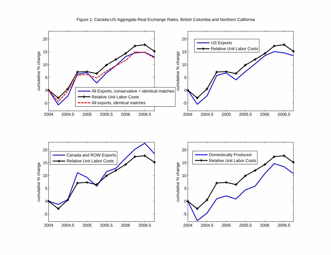
2004 2004.5 2005 2005.5 2006 2006.5
-5
0
5
10
15
20cu
mul
ativ
e %
cha
nge
All Exports, conservative + identical matchesRelative Unit Labor CostsAll exports, identical matches
2004 2004.5 2005 2005.5 2006 2006.5
-5
0
5
10
15
20
cum
ulat
ive
% c
hang
e
US ExportsRelative Unit Labor Costs
2004 2004.5 2005 2005.5 2006 2006.5
-5
0
5
10
15
20
cum
ulat
ive
% c
hang
e
Canada and ROW ExportsRelative Unit Labor Costs
Figure 1: Canada-US Aggregate-Real Exchange Rates, British Columbia and Northern California
2004 2004.5 2005 2005.5 2006 2006.5
-5
0
5
10
15
20
cum
ulat
ive
% c
hang
e
Domestically ProducedRelative Unit Labor Costs

2004.5 2005 2005.5 2006 2006.5
-15
-10
-5
0
5
10
Qua
rterly
Per
cent
age
Cha
nge
Price changes
Δ PUS region 1
Δ PUS region 2
Δ PCan region 1
Figure 2: Price Movements for a US Exported Product in the "Tea" Category
2004.5 2005 2005.5 2006 2006.5
-20
-15
-10
-5
0
5
10
15
20
Qua
rterly
Per
cent
age
Cha
nge
Product-level RERs
Δ Relative unit labor costs
Δ Qintra
Δ Qinter

-0.25 -0.2 -0.15 -0.1 -0.05 0 0.05 0.1 0.15 0.2 0.250
0.05
0.1
0.15
0.2
0.25
0.3All exported matched products, identical + conservative, British Columbia and North California
Δ Q intra CanΔ Q intra USΔ Q inter
Figure 3: Histogram of Movements of Product-Level Real Exchange Rates
-0.25 -0.2 -0.15 -0.1 -0.05 0 0.05 0.1 0.15 0.2 0.250
0.05
0.1
0.15
0.2
0.25
0.3
All domestically produced matched products, identical + conservative, British Columbia and North California
Δ Q intra CanΔ Q intra USΔ Q inter

2004 2004.5 2005 2005.5 2006 2006.5-5
0
5
10
15
20
% c
umul
ativ
e ch
ange
US exports
2004 2004.5 2005 2005.5 2006 2006.5-5
0
5
10
15
20Canadian exports
2004 2004.5 2005 2005.5 2006 2006.5-5
0
5
10
15
20Domestically produced
2004 2004.5 2005 2005.5 2006 2006.5-5
0
5
10
15
20Rest of the world exports
Figure 4: Model Aggregate Real Exchange Rates
Relative unit labor costsAggregate RER

Table 1: Descriptive Statistics
Panel A: Identical Matches
Center‐West Center‐West British NorthCanada US Columbia California
1 Expenditure share of matched products 0.04 0.05 0.04 0.06out of total expenditure
Expenditure share of products produced in:
2 U.S. 0.60 0.76 0.63 0.733 Canada 0.24 0.03 0.21 0.054 ROW (Same Country) 0.16 0.21 0.16 0.22
Number of products produced in:
5 U.S. 573 628 444 5436 Canada 128 39 105 237 ROW (Same Country) 332 302 179 234
Number of matched products by country‐of‐production set
8 US exports (produced in US for sales in Canada and US) 573 552 444 4809 Canada exports (produced in Canada for sales in Canada and US) 44 39 25 23
10 ROW Exports (produced in ROW for sales in Canada and US) 332 302 179 23411 Domestically produced (in Canada for Canada sales and in US for US sales) 84 76 80 63
12 Number of product categories 60 55 17 53
13 Number of pricing regions: 17 51 5 14
Panel B: Identical + Conservative Matches
Center‐West Center‐West British NorthCanada US Columbia California
14 Expenditure share of matched products 0.52 0.36 0.51 0.36out of total expenditure
Expenditure share of products produced in:
15 U.S. 0.29 0.89 0.30 0.8716 Canada 0.68 0.02 0.67 0.0117 ROW (Same Country) 0.03 0.09 0.03 0.11
Number of products produced in:
18 U.S. 1522 5278 1477 418519 Canada 1925 238 1727 16120 ROW (Same Country) 418 636 303 470
Number of matched products by country‐of‐production set
21 U.S. exports (produced in U.S. for sales in Canada and US) 5496 5496 4504 450422 Canada exports (produced in Canada for sales in Canada and U.S.) 191 191 124 12423 ROW exports (produced in ROW for sales in Canada and U.S.) 367 367 236 23624 Domestically produced (in Canada for Canada sales and in U.S. for U.S. sales) 5385 5385 4187 4187
25 Number of product categories 93 93 93 93
26 Number of pricing regions: 17 51 5 14
Center‐West includes all pricing regions in Canada (British Columbia, Alberta, and Manitoba), and 51 pricing regions in the U.S. located in California, Oregon, Idaho, Montana, and Wyoming

Table 2: Movements in Product‐Level Real‐Exchange Rates
Panel A: Identical + Conservative Matches, North California and British Columbia
All All Exports US Exports Can Exports ROW Exports Domestic
1 Stdintra US 0.06 0.06 0.06 0.08 0.08 0.07
2 Stdintra Can 0.05 0.05 0.05 0.04 0.07 0.05
3 Stdinter 0.13 0.11 0.10 0.14 0.14 0.13
4 Correlintra US 0.75 0.73 0.73 0.71 0.73 0.79
5 Correlintra Can 0.84 0.80 0.80 0.89 0.77 0.88
6 Correlinter 0.07 0.09 0.10 0.05 0.09 0.07
Panel B: Identical Matches, North California and British Columbia
All All Exports US Exports Can Exports ROW Exports Domestic
7 Stdintra US 0.09 0.09 0.09 0.08 0.10 0.07
8 Stdintra Can 0.07 0.08 0.07 0.04 0.09 0.05
9 Stdinter 0.13 0.13 0.12 0.09 0.15 0.10
10 Correlintra US 0.52 0.53 0.56 0.36 0.47 0.45
11 Correlintra Can 0.72 0.72 0.72 0.78 0.71 0.79
12 Correlinter 0.09 0.10 0.10 0.00 0.09 ‐0.03
Panel C: Identical Matches, Center‐West Canada and Center‐West US
All All Exports US Exports Can Exports ROW Exports Domestic
13 Stdintra US 0.07 0.07 0.07 0.06 0.09 0.06
14 Stdintra Can 0.07 0.07 0.06 0.03 0.09 0.05
15 Stdinter 0.13 0.13 0.12 0.08 0.15 0.10
16 Correlintra US 0.68 0.68 0.68 0.45 0.70 0.56
17 Correlintra Can 0.76 0.76 0.76 0.85 0.75 0.83
18 Correlinter 0.11 0.12 0.13 0.00 0.10 ‐0.06

Table 3: Movements in Product‐Level Real‐Exchange Rates, Robustness
All All exp. US exp. Can. exp. ROW exp. Domestic All All exp. US exp. Can. exp. ROW exp. Domestic
1 Stdintra US 0.06 0.06 0.05 0.10 0.07 0.07 0.06 0.06 0.06 0.09 0.09 0.07
2 Stdintra Can 0.04 0.04 0.03 0.02 0.08 0.04 0.04 0.04 0.04 0.05 0.07 0.04
3 Stdinter 0.13 0.11 0.11 0.17 0.14 0.15 0.12 0.11 0.11 0.15 0.14 0.13
4 Correlintra US 0.77 0.74 0.75 0.68 0.74 0.79 0.77 0.73 0.75 0.72 0.65 0.78
5 Correlintra Can 0.93 0.89 0.90 0.96 0.74 0.94 0.87 0.86 0.88 0.88 0.77 0.88
6 Correlinter 0.07 0.05 0.06 ‐0.04 0.09 0.09 0.07 0.06 0.05 0.08 0.08 0.07
All All exp. US exp. Can. exp. ROW exp. Domestic All All exp. US exp. Can. exp. ROW exp. Domestic
7 Stdintra US 0.08 0.08 0.08 0.10 0.09 0.08
8 Stdintra Can 0.04 0.05 0.04 0.04 0.07 0.04
9 Stdinter 0.12 0.11 0.11 0.15 0.15 0.12 0.12 0.11 0.11 0.20 0.15 0.13
10 Correlintra US 0.61 0.59 0.57 0.84 0.62 0.62
11 Correlintra Can 0.87 0.82 0.82 0.92 0.78 0.91
12 Correlinter 0.07 0.06 0.05 0.08 0.10 0.08 0.06 0.07 0.08 ‐0.03 0.06 0.05
All All exp. US exp. Can. exp. ROW exp. Domestic All All exp. US exp. Can. exp. ROW exp. Domestic
13 Stdintra US 0.06 0.06 0.05 0.09 0.07 0.06 0.07 0.07 0.07 0.09 0.07 0.07
14 Stdintra Can 0.04 0.04 0.04 0.03 0.05 0.04 0.05 0.04 0.05 0.06 0.07 0.05
15 Stdinter 0.12 0.11 0.11 0.21 0.13 0.13 0.19 0.19 0.23 0.19 0.21 0.20
16 Correlintra US 0.78 0.76 0.76 0.71 0.74 0.79 0.85 0.84 0.85 0.76 0.72 0.85
17 Correlintra Can 0.88 0.86 0.86 0.95 0.84 0.90 0.96 0.97 0.95 0.94 0.94 0.94
18 Correlinter 0.07 0.09 0.09 0.00 0.13 0.06 0.06 0.09 0.03 0.03 0.06 0.04
All All exp. US exp. Can. exp. ROW exp. Domestic All All exp. US exp. Can. exp. ROW exp. Domestic
19 Stdintra US 0.08 0.08 0.08 0.05 0.09 0.05 0.08 0.07 0.07 0.08 0.07 0.10
20 Stdintra Can 0.05 0.05 0.05 0.03 0.05 0.04 0.05 0.05 0.05 0.04 0.05 0.04
21 Stdinter 0.12 0.12 0.12 0.07 0.13 0.09 0.14 0.14 0.14 0.17 0.13 0.14
22 Correlintra US 0.73 0.73 0.73 0.59 0.71 0.77 0.75 0.75 0.75 0.89 0.77 0.75
23 Correlintra Can 0.80 0.80 0.81 0.70 0.76 0.82 0.85 0.83 0.83 0.81 0.05 0.87
24 Correlinter 0.06 0.07 0.07 0.15 0.06 ‐0.04 0.08 0.03 0.03 0.18 0.01 0.13
NC: Northern California, BC: British Columbia
H: Retail Prices, Identical + Conserv. Matches, NC and BC
C: One pricing region in Seattle and in British Columbia
E: Prices Demeaned by Category‐wide price
B: Center‐West pricing regions
D: Four pricing regions: BC, Manitoba, NC, Illinois
A: Liberal Matches
F: Weekly Prices
G: Retail Prices, Identical Matches, NC and BC

Table 4 : Baseline Parameterization: Parameter Values and Targets
Panel A: Parameter values
Parameters that determine trade patterns
1 K 1 28
2 K 2 4
3 K 3 5
4 D 1.585 D* 1.156 λ 0.357 θ 0.3
Parameters that determine price movements Uncorrelated Correlated demand shocks
8 σ z 0.054 0.034
9 0.780 0.33310 ρ a 0 0.64
Panel B: Targets
T d h S
z2/z
2 a2
Trade shares Source
11 Exports Can to US , share of US expenditures, selected industries 2% Source OECD12 Exports US to Can , share of Can expenditures, selected industries 25% Source OECD13 Average Exports ROW to Can, ROW to US, 10% Source OECD
share of US,Can expenditures, selected industries14 Expenditures in Nd / Expenditures in Nx1 and Nx2 , Canada 1% Our data
Prices
15 Standard deviation price changes, US exporters, 8% Our data average US and Canada, Region 2
16 Intra‐national correlation of price changes, US exporters 0.82 Our data average US and Canada , Region 2
17 International correlation of price changes, US exporters 0.08 Our data average US reference and Canada reference , Region 2
18 Canada‐US relative unit labor costs, overall apreciation 2004‐2006 15% OECD
z2/z
2 a2

Table 5: Quantitative Results, Baseline and Sensitivity Analysis
1 2 3 4 5 6 7
Baseline Correlated demand Small shocks Lower MP θ = 0.45 θ = 0.2 η = 2ρ a = 0 shocks, ρ a > 0 λ = 0.15
Panel A: Product‐level price statistics
US Exports
1 Correlation intranational prices 0.75 0.74 0.75 0.75 0.74 0.75 0.752 Correlation international prices 0.26 0.11 0.20 0.25 0.24 0.31 0.323 Variance inter / intra RER 1.72 1.87 1.90 1.74 1.73 1.67 1.68
Canadian Exports
4 Correlation intranational prices 0.73 0.73 0.75 0.74 0.73 0.74 0.705 Correlation international prices 0.19 0.08 0.14 0.18 0.16 0.22 0.206 Variance inter / intra RER 1.85 1.96 1.99 1.90 1.85 1.84 1.65
ROW Exports
7 Correlation intranational prices 0.74 0.74 0.76 0.74 0.74 0.75 0.728 Correlation international prices 0.17 0.08 0.12 0.14 0.15 0.21 0.229 Variance inter / intra RER 1 87 1 95 2 02 1 92 1 86 1 86 1 719 Variance inter / intra RER 1.87 1.95 2.02 1.92 1.86 1.86 1.71
Domestically produced
10 Correlation intranational prices 0.74 0.74 0.76 0.74 0.74 0.75 0.7111 Correlation international prices 0.18 0.07 0.14 0.14 0.15 0.22 0.1112 Variance inter / intra RER 1.85 1.94 2.00 1.90 1.85 1.81 1.81
Panel B: Aggregate price statistics
Change in RER / Change in relative costs
13 US Exports 0.64 0.63 0.71 0.64 0.66 0.60 0.53
14 Canadian Exports 0.75 0.73 0.81 0.76 0.77 0.71 0.69
15 ROW Exports 0.76 0.74 0.83 0.79 0.78 0.72 0.67
16 Domestically produced 0.78 0.79 0.81 0.83 0.80 0.75 0.87
In cases 2‐7 we adjust the remaining parameters to match the other calibration targets.