Embed Size (px)
Citation preview

UNIVERSITAT POLITÈCNICA DE CATALUNYA
Programa de Doctorat:
AUTOMÀTICA, ROBÒTICA I VISIÓ
Tesi Doctoral
Understanding Human-Centric Images:
From Geometry to Fashion
Edgar Simo Serra
Directors:Francesc Moreno Noguer
Carme Torras
May 2014


Abstract
Understanding humans from photographs has always been a fundamentalgoal of computer vision. Early works focused on simple tasks such as de-tecting the location of individuals by means of bounding boxes. As the fieldprogressed, harder and more higher level tasks have been undertaken. Forexample, from human detection came the 2D and 3D human pose estima-tion in which the task consisted of identifying the location in the image orspace of all different body parts, e.g., head, torso, knees, arms, etc. Humanattributes also became a great source of interest as they allow recognizingindividuals and other properties such as gender or age. Later, the attentionturned to the recognition of the action being performed. This, in general,relies on the previous works on pose estimation and attribute classification.Currently, even higher level tasks are being conducted such as predictingthe motivations of human behaviour or identifying the fashionability of anindividual from a photograph.
In this thesis we have developed a hierarchy of tools that cover all theserange of problems, from low level feature point descriptors to high levelfashion-aware conditional random fields models, all with the objective ofunderstanding humans from monocular RGB images. In order to buildthese high level models it is paramount to have a battery of robust andreliable low and mid level cues. Along these lines, we have proposed twolow-level keypoint descriptors: one based on the theory of the heat diffu-sion on images, and the other that uses a convolutional neural network tolearn discriminative image patch representations. We also introduce distinctlow-level generative models for representing human pose: in particular wepresent a discrete model based on a directed acyclic graph and a continuousmodel that consists of poses clustered on a Riemannian manifold. As midlevel cues we propose two 3D human pose estimation algorithms: one thatestimates the 3D pose given a noisy 2D estimation, and an approach thatsimultaneously estimates both the 2D and 3D pose. Finally, we formulatehigher level models built upon low and mid level cues for understanding hu-mans from single images. Concretely, we focus on two different tasks in thecontext of fashion: semantic segmentation of clothing, and predicting thefashionability from images with metadata to ultimately provide fashion ad-vice to the user.
In summary, to robustly extract knowledge from images with the pres-ence of humans it is necessary to build high level models that integrate lowand mid level cues. In general, using and understanding strong features iscritical for obtaining reliable performance. The main contribution of thisthesis is in proposing a variety of low, mid and high level algorithms forhuman-centric images that can be integrated into higher level models forcomprehending humans from photographs, as well as tackling novel fashion-oriented problems.
Keywords: human-centric imaging, feature descriptors, human pose es-timation, generative models, semantic segmentation, conditional randomfields, convolutional neural networks, fashion.


Acknowledgements
I would like to firstly thank both my advisors Francesc and Carme, to whom I owe thisopportunity. I would also like to thank everyone who supported me during this longjourney, and in particular, Rasputin and Nuryev.
This work has been partly sponsored by the following:
- A four-year PhD scholarship (BES-2012-054905).
- A four-month scholarship to visit the Toyota Technological Institute at Chicago(EEBB-I-14-08177).
- A four-month scholarship to visit the Nakamura Laboratory in Japan (EEBB-I-15-09283).
- Projects CINNOVA (201150E088), PAU+ (DPI2011-27510), ViSEN (ERA-NetChistera PCIN-2013-047), and Intellact (FP7-ICT2009-6-269959).
- My own stubbornness.
iii


In loving memory of Misi


Contents
Contents vii
List of Figures ix
List of Tables xii
1 Introduction 11.1 Contributions . . . . . . . . . . . . . . . . . . . . . . . . . . . . . . . . . 2
Publications . . . . . . . . . . . . . . . . . . . . . . . . . . . . . . . . . . 31.2 Thesis Overview . . . . . . . . . . . . . . . . . . . . . . . . . . . . . . . 4
2 Overview 72.1 Low Level Cues . . . . . . . . . . . . . . . . . . . . . . . . . . . . . . . . 7
Image Features . . . . . . . . . . . . . . . . . . . . . . . . . . . . . . . . 8Simple Priors . . . . . . . . . . . . . . . . . . . . . . . . . . . . . . . . . 10
2.2 Mid Level Cues . . . . . . . . . . . . . . . . . . . . . . . . . . . . . . . . 10Image Features . . . . . . . . . . . . . . . . . . . . . . . . . . . . . . . . 10Prior Models . . . . . . . . . . . . . . . . . . . . . . . . . . . . . . . . . 13Bag-of-Words . . . . . . . . . . . . . . . . . . . . . . . . . . . . . . . . . 14
2.3 High Level Cues . . . . . . . . . . . . . . . . . . . . . . . . . . . . . . . 142.4 Machine Learning Models . . . . . . . . . . . . . . . . . . . . . . . . . . 14
Logistic Regression . . . . . . . . . . . . . . . . . . . . . . . . . . . . . . 15Support Vector Machines . . . . . . . . . . . . . . . . . . . . . . . . . . 15Deep Networks . . . . . . . . . . . . . . . . . . . . . . . . . . . . . . . . 16Conditional Random Fields . . . . . . . . . . . . . . . . . . . . . . . . . 18
3 Feature Point Descriptors 213.1 Introduction . . . . . . . . . . . . . . . . . . . . . . . . . . . . . . . . . . 213.2 Deformation and Illumination Invariant (DaLI) Descriptor . . . . . . . . 23
Related Work . . . . . . . . . . . . . . . . . . . . . . . . . . . . . . . . . 25Deformation and Light Invariant Descriptor . . . . . . . . . . . . . . . . 26Deformation and Varying Illumination Dataset . . . . . . . . . . . . . . 34Results . . . . . . . . . . . . . . . . . . . . . . . . . . . . . . . . . . . . . 39
3.3 Deep Architectures for Descriptors . . . . . . . . . . . . . . . . . . . . . 49
vii

viii Contents
Related Work . . . . . . . . . . . . . . . . . . . . . . . . . . . . . . . . . 50Learning Deep Descriptors . . . . . . . . . . . . . . . . . . . . . . . . . . 50Results . . . . . . . . . . . . . . . . . . . . . . . . . . . . . . . . . . . . . 53
3.4 Summary . . . . . . . . . . . . . . . . . . . . . . . . . . . . . . . . . . . 59
4 Generative 3D Human Pose Models 634.1 Introduction . . . . . . . . . . . . . . . . . . . . . . . . . . . . . . . . . . 634.2 Related Work . . . . . . . . . . . . . . . . . . . . . . . . . . . . . . . . . 654.3 Linear Latent Model . . . . . . . . . . . . . . . . . . . . . . . . . . . . . 67
Deformation Modes . . . . . . . . . . . . . . . . . . . . . . . . . . . . . . 67Results . . . . . . . . . . . . . . . . . . . . . . . . . . . . . . . . . . . . . 68
4.4 Directed Acyclic Graphs . . . . . . . . . . . . . . . . . . . . . . . . . . . 69Discrete Joint Model . . . . . . . . . . . . . . . . . . . . . . . . . . . . . 70Results . . . . . . . . . . . . . . . . . . . . . . . . . . . . . . . . . . . . . 71
4.5 Geodesic Finite Mixture Models . . . . . . . . . . . . . . . . . . . . . . . 73Method . . . . . . . . . . . . . . . . . . . . . . . . . . . . . . . . . . . . 74Results . . . . . . . . . . . . . . . . . . . . . . . . . . . . . . . . . . . . . 77
4.6 Summary . . . . . . . . . . . . . . . . . . . . . . . . . . . . . . . . . . . 80
5 3D Human Pose Estimation 835.1 Introduction . . . . . . . . . . . . . . . . . . . . . . . . . . . . . . . . . . 835.2 Related work . . . . . . . . . . . . . . . . . . . . . . . . . . . . . . . . . 855.3 3D Pose Estimation from Noisy 2D Observations . . . . . . . . . . . . . 86
Method . . . . . . . . . . . . . . . . . . . . . . . . . . . . . . . . . . . . 87Results . . . . . . . . . . . . . . . . . . . . . . . . . . . . . . . . . . . . . 92
5.4 Joint 2D and 3D Pose Estimation . . . . . . . . . . . . . . . . . . . . . . 94Method . . . . . . . . . . . . . . . . . . . . . . . . . . . . . . . . . . . . 95Results . . . . . . . . . . . . . . . . . . . . . . . . . . . . . . . . . . . . . 100
5.5 Summary . . . . . . . . . . . . . . . . . . . . . . . . . . . . . . . . . . . 102
6 Probabilistically Modelling Fashion 1056.1 Introduction . . . . . . . . . . . . . . . . . . . . . . . . . . . . . . . . . . 1056.2 Segmentation of Garments in Fashion Images . . . . . . . . . . . . . . . 107
Related Work . . . . . . . . . . . . . . . . . . . . . . . . . . . . . . . . . 108Clothing a Person . . . . . . . . . . . . . . . . . . . . . . . . . . . . . . . 109Experimental Evaluation . . . . . . . . . . . . . . . . . . . . . . . . . . . 115
6.3 Modelling Fashionability . . . . . . . . . . . . . . . . . . . . . . . . . . . 120Related Work . . . . . . . . . . . . . . . . . . . . . . . . . . . . . . . . . 122Fashion144k Dataset . . . . . . . . . . . . . . . . . . . . . . . . . . . . . 123Discovering Fashion from Weak Data . . . . . . . . . . . . . . . . . . . . 126Experimental Evaluation . . . . . . . . . . . . . . . . . . . . . . . . . . . 129
6.4 Summary . . . . . . . . . . . . . . . . . . . . . . . . . . . . . . . . . . . 136
7 Conclusions 1377.1 Future Work . . . . . . . . . . . . . . . . . . . . . . . . . . . . . . . . . 1387.2 Trends in Computer Vision and Machine Learning . . . . . . . . . . . . 139
Bibliography 141

List of Figures
2.1 Human detection with HOG descriptors . . . . . . . . . . . . . . . . . . . . 10
2.2 Examples of saliency detection . . . . . . . . . . . . . . . . . . . . . . . . . 11
2.3 Architecture of a convolutional neural network . . . . . . . . . . . . . . . . 12
2.4 2D human pose estimation . . . . . . . . . . . . . . . . . . . . . . . . . . . . 13
2.5 Convolutional Neural Network architecture . . . . . . . . . . . . . . . . . . 18
2.6 Example of a Conditional Random Field model . . . . . . . . . . . . . . . . 20
3.1 SIFT descriptor . . . . . . . . . . . . . . . . . . . . . . . . . . . . . . . . . . 22
3.2 Comparing DaLI against SIFT, DAISY, LIOP, and GIH. . . . . . . . . . . . 23
3.3 Visualization of a DaLI descriptor. . . . . . . . . . . . . . . . . . . . . . . . 24
3.4 Flowchart of the algorithm used to calculate the DaLI and DaLI-PCA de-scriptors . . . . . . . . . . . . . . . . . . . . . . . . . . . . . . . . . . . . . . 25
3.5 DaLI descriptor . . . . . . . . . . . . . . . . . . . . . . . . . . . . . . . . . . 27
3.6 Invariance of the DaLI and DI descriptors to non-rigid deformations andillumination changes . . . . . . . . . . . . . . . . . . . . . . . . . . . . . . . 29
3.7 Evaluation of the descriptor robustness on synthetic sequences . . . . . . . 30
3.8 Representation of an image patch . . . . . . . . . . . . . . . . . . . . . . . . 32
3.9 Different mesh triangulations . . . . . . . . . . . . . . . . . . . . . . . . . . 32
3.10 Preserving edge information . . . . . . . . . . . . . . . . . . . . . . . . . . . 34
3.11 Deformable and varying illumination dataset . . . . . . . . . . . . . . . . . 36
3.12 Extracting patches from points of interest . . . . . . . . . . . . . . . . . . . 37
3.13 DaLI performance for different parameter values So, β, σ and wmax . . . . . 38
3.14 The first 7 frequencies of the first 20 components of the PCA basis . . . . . 40
3.15 PCA approximation of the DaLI descriptor . . . . . . . . . . . . . . . . . . 41
3.16 Mean detection rates obtained by scaling regions of interest with differentfactors. . . . . . . . . . . . . . . . . . . . . . . . . . . . . . . . . . . . . . . 42
3.17 Detection rate when simultaneously varying deformation level and illumina-tion conditions . . . . . . . . . . . . . . . . . . . . . . . . . . . . . . . . . . 43
3.18 DaLI descriptor results for varying only deformation or illumination . . . . 44
3.19 Sample results from the dataset . . . . . . . . . . . . . . . . . . . . . . . . . 45
3.20 True positive, false positive, false negative and true negative image patch pairs 46
3.21 Mean detection accuracy on two real world videos . . . . . . . . . . . . . . 47
3.22 Overview of the network architectures used . . . . . . . . . . . . . . . . . . 51
ix

x List of Figures
3.23 Pairs of corresponding samples from the Multi-view Stereo Correspondencedataset . . . . . . . . . . . . . . . . . . . . . . . . . . . . . . . . . . . . . . 53
3.24 Precision-recall curves for different network architectures . . . . . . . . . . . 55
3.25 Precision-recall curves for different network hyperparameters . . . . . . . . 55
3.26 Precision-recall curves for different levels of mining . . . . . . . . . . . . . . 57
3.27 Precision-recall curves for different number of filters and fully-connected layers 57
3.28 Precision-recall curves for the generalized results over the three dataset splits 58
3.29 Samples of matches retrieved with our descriptor . . . . . . . . . . . . . . . 60
4.1 Example of a GPDM with a 3-dimensional latent space. . . . . . . . . . . . 64
4.2 Examples of 3D body shape scans . . . . . . . . . . . . . . . . . . . . . . . 66
4.3 Effect of σthreshold in linear latent models. . . . . . . . . . . . . . . . . . . . 68
4.4 Dimensionality of the Linear Latent Space . . . . . . . . . . . . . . . . . . . 69
4.5 Directed Acyclic Graph models for 3D human pose . . . . . . . . . . . . . . 71
4.6 Directed Acyclic Graph modeltraining and sampling . . . . . . . . . . . . . 72
4.7 Geodesics and mixture models . . . . . . . . . . . . . . . . . . . . . . . . . 73
4.8 Sampling from the Geodesic Finite Mixture Model . . . . . . . . . . . . . . 78
4.9 Human pose regression with the GFMM . . . . . . . . . . . . . . . . . . . . 80
5.1 Example of a multiview 3D pose estimation approach . . . . . . . . . . . . 84
5.2 Convolutional Neural Network for 3D Pose Estimation . . . . . . . . . . . . 85
5.3 3D human pose estimation from noisy observations. . . . . . . . . . . . . . . 86
5.4 Flowchart of the method for obtaining 3D human pose from single images . 87
5.5 Exploration of the solution space . . . . . . . . . . . . . . . . . . . . . . . . 91
5.6 Exploring the space of articulated shapes. . . . . . . . . . . . . . . . . . . . 91
5.7 Choosing human-like hypothesis via anthropomorphism. . . . . . . . . . . . 92
5.8 Comparison of different error functions for 3D human pose estimation. . . . 93
5.9 3D Human Pose Estimation Results . . . . . . . . . . . . . . . . . . . . . . 95
5.10 Results on the TUD Stadmitte sequence. . . . . . . . . . . . . . . . . . . . . 96
5.11 Simultaneous estimation of 2D and 3D pose. . . . . . . . . . . . . . . . . . . 96
5.12 Overview of our method for simultaneous 2D and 3D pose estimation . . . . 97
5.13 2D part detectors. . . . . . . . . . . . . . . . . . . . . . . . . . . . . . . . . 98
5.14 Sample frames from the HumanEva dataset. . . . . . . . . . . . . . . . . . . 101
5.15 Two sample frames from the TUD Stadmitte sequence . . . . . . . . . . . . 102
6.1 Garment segmentation example . . . . . . . . . . . . . . . . . . . . . . . . . 106
6.2 Fine-grained annotations of the Fashionista dataset. . . . . . . . . . . . . . 107
6.3 Visualization of object masks and limbs. . . . . . . . . . . . . . . . . . . . . 110
6.4 Visualization of clothelets . . . . . . . . . . . . . . . . . . . . . . . . . . . . 111
6.5 Wordnet-based similarity function . . . . . . . . . . . . . . . . . . . . . . . 114
6.6 Confusion matrix for our approach on the Fashionista v0.3 dataset. . . . . . 116
6.7 Per class results for our model. . . . . . . . . . . . . . . . . . . . . . . . . . 118
6.8 Visualization of different features . . . . . . . . . . . . . . . . . . . . . . . . 120
6.9 Qualitative clothing segmentation results . . . . . . . . . . . . . . . . . . . 121
6.10 Example of an outfit recommendation . . . . . . . . . . . . . . . . . . . . . 122
6.11 Anatomy of a post from the Fashion144k dataset . . . . . . . . . . . . . . . 122
6.12 Normalization of votes . . . . . . . . . . . . . . . . . . . . . . . . . . . . . . 126
6.13 Visualization of the density of posts and fashionability by country . . . . . 126

List of Figures xi
6.14 An overview of the CRF model and the features used by each of the nodes . 1276.15 Illustration of the type of deep network architecture used to learn features . 1286.16 Visualization of mean beauty and dominant ethnicity by country . . . . . . 1306.17 True and false positive fashionability prediction examples . . . . . . . . . . 1326.18 Visualization of the dominant latent clusters . . . . . . . . . . . . . . . . . . 1336.19 Visualizing pairwise potentials between nodes in the CRF . . . . . . . . . . 1346.20 Examples of recommendations provided for our model . . . . . . . . . . . . 1356.21 Visualization of the temporal evolution of the different trends in Manila and
Los Angeles . . . . . . . . . . . . . . . . . . . . . . . . . . . . . . . . . . . . 135

List of Tables
2.1 Different types of computer vision cues . . . . . . . . . . . . . . . . . . . . . 8
3.1 DaLI computation time and mesh complexity for different triangulations . . 33
3.2 DaLI parameters . . . . . . . . . . . . . . . . . . . . . . . . . . . . . . . . . 35
3.3 Evaluation results on the dataset for all descriptors . . . . . . . . . . . . . . 46
3.4 Comparison of performance and descriptor size . . . . . . . . . . . . . . . . 48
3.5 Effect of normalizing image patches for various descriptors . . . . . . . . . . 49
3.6 Effect of network architectures . . . . . . . . . . . . . . . . . . . . . . . . . 54
3.7 Comparison of network hyperparameters . . . . . . . . . . . . . . . . . . . . 54
3.8 Effect of mining samples on performance . . . . . . . . . . . . . . . . . . . . 56
3.9 Effect of number of filters and fully-connected layer . . . . . . . . . . . . . . 56
3.10 Precision-recall area under the curve for the generalized results . . . . . . . 58
4.1 Comparison of generative pose models . . . . . . . . . . . . . . . . . . . . . 66
4.2 Influence of the number of latent states . . . . . . . . . . . . . . . . . . . . 71
4.3 Comparison of the Geodesic Finite Mixture Model with other approaches. . 79
5.1 Comparison of results on the HumanEva dataset. . . . . . . . . . . . . . . . 94
5.2 Results on the HumanEva dataset. . . . . . . . . . . . . . . . . . . . . . . . 100
5.3 Comparison against the state-of-the-art. . . . . . . . . . . . . . . . . . . . . 102
6.1 Overview of the different types of potentials used in the proposed CRF model109
6.2 Comparison against the state-of-the-art. . . . . . . . . . . . . . . . . . . . . 115
6.3 Evaluation on the foreground segmentation task . . . . . . . . . . . . . . . . 117
6.4 Influence of pose. . . . . . . . . . . . . . . . . . . . . . . . . . . . . . . . . . 117
6.5 Oracle performance for different superpixel levels . . . . . . . . . . . . . . . 118
6.6 Different results using only unary potentials in our model . . . . . . . . . . 118
6.7 Importance of the different potentials in the full model . . . . . . . . . . . . 119
6.8 Statistics of the Fashion144k dataset . . . . . . . . . . . . . . . . . . . . . . 124
6.9 Mean fashionability of cities with at least 1000 posts . . . . . . . . . . . . . 125
6.10 Overview of the different features used . . . . . . . . . . . . . . . . . . . . . 125
6.11 Effect of various attributes on the fashionability . . . . . . . . . . . . . . . . 130
6.12 Fashionability prediction results . . . . . . . . . . . . . . . . . . . . . . . . . 131
6.13 Evaluation of features for predicting fashionability . . . . . . . . . . . . . . 132
xii
Chapter 1
Introduction
I may not have gone where Iintended to go, but I think I haveended up where I intended to be.
Douglas Adams
Computer vision is a relatively new field with roughly half a century of tradition.It is a well known anecdote that it originally started out as a summer project for a firstyear undergraduate student in 1966, whose task was to “connect a television camera toa computer and get the machine to describe what it sees.” Had computer vision notbeen grossly underestimated and the project succeeded, this thesis would not have beenpossible and the author would be likely enjoying a long drink at the beach. However,seeing that this thesis is indeed finally completed, we come to the conclusion the projectwas not able to complete its ambitious task. Not only that, currently computer visionis a thriving field that is getting closer and closer to solving the 1966 summer problem.
In the beginning, computer vision was seen as more of a mathematical problem,which was additionally limited by the computational resources of the time. Duringthat period, many of the tools and basic approaches we still use today were developed.Only in the last decade has the technology advanced sufficiently to tackle lofty computervision problems and obtain reliable results that are making it into real world applicationseverywhere. One may argue that this started with the SIFT descriptor (Lowe, 2004),the most cited paper in computer vision1, which eventually allowed the appearance ofother notable works such as the deformable parts model (Felzenszwalb et al., 2008) forobject detection. These models began to obtain significant results in identifying objectsin natural photographs.
With the progress of time, datasets have increased in size and machine learning hasplayed a larger and larger role in computer vision, to the point that it has now becomean indispensable tool. One of the most important recent breakthroughs has been theuse of Convolutional Neural Networks (CNN) for classification (Krizhevsky et al., 2012)
1Indeed, as it is common among computer vision researchers, we compulsively track the number ofcitations the SIFT paper has, which at the time of this writing is of 28,407 citations.
1

2 Chapter 1. Introduction
which has outperformed existing approaches by a large margin. This has created animportant resurgence of Artificial Neural Networks (ANN) in computer vision, as theyare the basis for these techniques. In compliance with the current trends we rely heavilyon machine learning throughout this thesis.
One particular area of computer vision is the understanding of human-centric im-ages. This encompasses many different problems such as detection of individuals, 2D/3Dpose estimation, attribute prediction, gaze prediction, clothing segmentation, etc. Inparticular, tasks such as face detection are already a reality and omnipresent for almostall types of digital cameras, while other problems such as assessing image memorabilityare still in their incipiency. In this thesis we focus on 3D human pose estimation, clothessegmentation, and predicting fashionability. For this purpose we have developed gen-erative models for 3D human pose and feature point descriptors, which by themselvesare unable to perform these tasks, but play a fundamental role in the algorithms thatare able to do so.
Although our ultimate objective is higher level comprehension of human-centricimages and problems such as the estimation of fashionability, this is unable to be per-formed without leveraging robust low level cues. Therefore it is critical to have a stronggrasp of mid and low level algorithms. For this purpose we exploit a swath of existingfeatures while supplementing them with our own. We show that our features are ableto complement the existing ones while palliating their deficiencies.
1.1 Contributions
We organize the contributions into four groups: feature point descriptors, generative 3Dhuman pose models, 3D human pose estimation, and probabilistically modelling fashion.
1. Feature point descriptors. We propose two different feature point descriptors:one based on heat diffusion and another based on Convolutional Neural Networks(CNN). In the first approach we model the image patch as a 3D surface. After-wards we calculate the heat diffusion for logarithmically sampled time intervalsand perform a Fast Fourier Transform on the resulting heat maps. We show thatthis approach is robust to both deformation and illumination changes. This de-scriptor, which we call DaLI , was published in (Simo-Serra et al., 2015b). Thesecond work consists of using CNN to learn discriminative representations of im-age patches. This is done by using a Siamese CNN architecture, trained withpairs of corresponding patches. We propose learning with a sampling-based ap-proach that in combination with heavy mining, which we denote “fracking”, is ableto significantly outperform hand-crafted features. This work is currently undersubmission (Simo-Serra et al., 2014c).
2. Generative 3D human pose models. We present two different generativemodels for parameterizing the 3D human pose: a Directed Acyclic Graph (DAG)and a mixture model for Riemannian manifolds. The DAG model uses discrete 3Dposes obtained from clustering and learns the joint distribution of the resulting 3Dposes and a latent space. By not having any loops, it is possible to efficiently mapfrom the latent pose space to the 3D space and vice versa. This work was publishedas part of (Simo-Serra et al., 2012). For the second approach we model the 3Dhuman pose by considering that it can be represented as data on a Riemannianmanifold. This model is shown to preserve physical properties, such as distances

1.1. Contributions 3
between joints, much better than competing approaches. Additionally, we showthat this scales well to large datasets and allows real-time sampling from themodel. This work was published in (Simo-Serra et al., 2014b), with an extensionfor estimating velocities published in (Simo-Serra et al., 2015c).
3. 3D human pose estimation. We propose two different algorithms for 3D hu-man pose estimation from single monocular images. In the first work we assumewe have a noisy estimation of the 2D human pose and use a linear formulationthat allows us to project forward these estimations to the 3D space. We then usethe distances between the 3D joints to estimate the anthropomorphism of the hy-potheses and obtain a final solution. This work was published in (Simo-Serraet al., 2012). The second approach performs the 2D and 3D human pose esti-mation jointly in a single probabilistic framework. This is done by extending thepictorial structures Bayesian formulation (Felzenszwalb and Huttenlocher, 2005)to 3D, which naturally leads to a hybrid generative-discriminative model. To esti-mate the 3D pose we sample from a generative 3D pose model and then evaluatethe hypotheses using a bank of discriminative 2D part detectors. We perform thisalternate optimization until convergence. This work was published in (Simo-Serraet al., 2013).
4. Probabilistically modelling fashion. We finally tackle two different problemsin the context of fashion: semantic segmentation of clothing, and predicting thefashionability of people in images. In the first problem we attempt to do fine-grained recognition of garments in an image. We propose a Conditional RandomFields (CRF) model that labels the different superpixels in the image. This is doneby leveraging a set of strong unary potentials in combination with flexible pairwisepotentials that are able to significantly outperform the state-of-the-art. This workwas published in (Simo-Serra et al., 2014a). For the second problem of estimatingfashionability, we have created a novel large dataset called Fashion144k generatedby crawling posts from the largest online social fashion website. We aggregatevotes or “likes” as a proxy for the fashionability of the posts and propose a largeassortment of features that we compress using a deep Neural Network. Finallywe interlace the features using a CRF model. The resulting model is then ableto naturally learn different types of users, outfits, and settings, which are usedto predict the fashionability of a post, and even give fashion advice. This workwas published in (Simo-Serra et al., 2015a). Both these last two works are thefruition of collaborating with Prof. Raquel Urtasun and Prof. Sanja Fidler, fromthe University of Toronto.
Our focus is on high performance, and when necessary, fast models. We publish thecode and the datasets when possible2 in order to ensure our contributions are beneficialto the community. We hope this will encourage other researchers to use and compareagainst our approaches.
Publications
The following is a list of the publications derived from this thesis:
2http://www.iri.upc.edu/people/esimo/

4 Chapter 1. Introduction
Simo-Serra, E., Ramisa, A., Alenyà, G., Torras, C., and Moreno-Noguer, F.Single Image 3D Human Pose Estimation from Noisy Observations. In IEEEConference on Computer Vision and Pattern Recognition, 2012.
Simo-Serra, E., Quattoni, A., Torras, C., and Moreno-Noguer, F. A Joint Modelfor 2D and 3D Pose Estimation from a Single Image. In IEEE Conference onComputer Vision and Pattern Recognition, 2013.
Simo-Serra, E., Torras, C., and Moreno-Noguer, F. Geodesic Finite MixtureModels. In British Machine Vision Conference, 2014.
Simo-Serra, E., Fidler, S., Moreno-Noguer, F., and Urtasun, R. A High Per-formance CRF Model for Clothes Parsing. In Asian Conference on ComputerVision, 2014.
Simo-Serra, E., Torras, C., and Moreno-Noguer, F. DaLI: Deformation andLight Invariant Descriptor. International Journal of Computer Vision, 1:1–1,2015.
Simo-Serra, E., Torras, C., and Moreno-Noguer, F. Lie Algebra-Based Kine-matic Prior for 3D Human Pose Tracking. In Machine Vision and Applications,2015.
Simo-Serra, E., Trulls, E., Ferraz, L., Kokkinos, I., and Moreno-Noguer, F.Fracking Deep Convolutional Image Descriptors. In International Conference onLearning Representations, 2015.
Simo-Serra, E., Fidler, S., Moreno-Noguer, F., and Urtasun, R. Neuroaestheticsin Fashion: Modeling the Perception of Fashionability. In IEEE Conference onComputer Vision and Pattern Recognition, 2015.
Additionally a publication is still under submission
Simo-Serra, E., Trulls, E., Ferraz, L., Kokkinos, I., and Moreno-Noguer, F.Fracking Deep Convolutional Image Descriptors. arXiv preprint arXiv:1412.6537,2014.
1.2 Thesis Overview
We group the work done conceptually into four major chapters as done for our contri-butions and then organize them from low to high level. Each of these chapters has anintroductory section, several sections explaining different techniques, each correspond-ing roughly to a single publication, and a summary of the work. We additionally includea chapter to give an overview of our efforts as well as establishing some groundwork forsome techniques we will use throughout the thesis. Finally the last chapter provides ageneral wrap-up and concludes the thesis.

1.2. Thesis Overview 5
Chapter 2: Overview. This introductory chapter gives a high level overview of thecurrent state of the art of computer vision for human-centric images. We alsointroduce basic concepts of tools that we will use throughout the thesis.
Chapter 3: Feature Point Descriptors. This chapter focuses on our work on fea-ture point descriptors. It gives a short introduction and then has two majorsections that cover our 2015 IJCV and a paper under submission respectively.
Chapter 4: Generative Models for 3D Human Pose. This chapter focuses on thethree different 3D human pose models that we use in the rest of the thesis, espe-cially in Chapter 5. We first give an introduction followed by an in-depth reviewof models used in the past decade. The following two sections refer to the modelsused in our 2012 and 2013 CVPR papers. Afterward, we describe the approachof our 2014 BMVC paper in detail. We conclude with a summary of the differentmodels.
Chapter 5: 3D Human Pose Estimation. This chapter focuses on our two approachesfor estimating 3D human pose from single images. We first overview the ap-proaches and elaborate on the related work in the field. The following two sec-tions are devoted to our 2012 and 2013 CVPR papers, respectively. Lastly, wesummarize the results.
Chapter 6: Probabilistically Modelling Fashion. In this chapter we look at theproblem of modelling fashion. We start with the motivation of this problem andits impact in society before going into details of our 2014 ACCV and 2015 CVPRpapers, respectively. The results are summarized at the end.
Chapter 7: Conclusions. The last chapter gives a high-level discussion of our con-tributions, how our work stands in the field, and current developments. We alsopose open questions and sketch directions for future research.


Chapter 2
Overview
Scientific progress goes “boink”?
Hobbes
In this thesis we attempt to tackle very challenging high level computer visionproblems. In order to do this, it is necessary to rely on robust low and mid level cues.In this chapter we will explain and give notions of the different cues and algorithms thatcan form part of these high level computer vision models. Of course the concepts of highand low are relative. In this chapter, and by extension the rest of this thesis, we shallconsider as high level models those that perform tasks such as the ones we will presentin Chapter 6, i.e., semantic segmentation of clothing and predicting fashionability froman image. Mid level cues will include pose estimation models such as those presentedin Chapter 5 and foreground-background segmentation algorithms. Finally, low levelcues will refer to features such as the prior distributions we describe in Chapter 4 orthe feature point descriptors we will present in the next chapter.
We shall additionally discuss several machine learning models used throughout thisthesis. In particular we will focus on logistic regression classifiers, Support VectorMachines (SVM), deep networks, and Conditional Random Fields (CRF). We shallformulate the different models, explain how they can be learnt, and briefly state someusage cases and applications of them.
This overview is not meant to be an exhaustive list of all the different cues andmachine learning models commonly used in computer vision. Instead, it is meant tobe a rough overview with a focus on the tasks considered in this thesis. A list of thedifferent cues we will discuss and their relationship to this thesis can be seen in Table 2.1.
This chapter is divided into four sections that address low, mid, high level cues, andmachine learning models, respectively.
2.1 Low Level Cues
We understand low level cues as simple features or priors that do not encode veryprolific information. They are meant to be “austere” and fast to compute, and are
7

8 Chapter 2. Overview
Level Feature Type C3 C4 C5 C6
Low
Colour Maps X X
Gabor Filter Maps X
Edge Detector Maps
Region Histogram Regions X
Descriptors Sparse, Maps X X X
PDF Prior Likelihood Prior X X X
Mid
Detectors Maps, Bounding Boxes X X
Foreground Segmentation Maps X
Saliency Maps
Order 2 Pooling Regions X
GIST Image
CNN Regions, Image X
Pose Spatial Prior X X
Attributes Generic X
Bag-of-Words Regions, Image X
High Semantic Segmentation Maps X
Table 2.1: Different types of computer vision cues. Overview of some commonlyused cues in computer vision and their relationship with this thesis. We categorizethem into low, mid and high level cues and based on their types. “Maps” generate2D or 3D matrices where a value or vector corresponds to each pixel, respectively.“Regions” correspond to larger areas such as superpixels. “Image” type cues providea single vector that corresponds to the entire image. In the right four columns weindicate to which chapter the cue relates to.
always integrated into some larger model as they, by themselves, are unable to completeany task. However, this does not mean they are useless. For certain problems, just bycombining and leveraging different weak low level cues it is possible to obtain significantperformance. As an example we refer to the approach of (Krähenbühl and Koltun,2011) that performs semantic segmentation with good results by only employing simplecolor features with some smoothing terms in a Conditional Random Fields framework.
Image Features
There are a variety of potential low level image features. The most simple one is todirectly use the RGB color values. This is most commonly used in Convolutional NeuralNetworks (Krizhevsky et al., 2012) after normalizing the values, that is, subtracting themean and dividing by the standard deviation of the pixel values. It is also possible toconvert the RGB values to other color spaces such as HSV, YUV or CIE L*a*b. Ingeneral, it is not clear which color space is the best for a specific application and thusit requires experimental validation.

2.1. Low Level Cues 9
Since individual pixels do not contain much information, it is standard to insteadgroup them into different regions which conceptually correspond to parts of the sameobject in the image (Achanta et al., 2012). This grouping is known as pooling and hastwo major effects: it first allows a much more efficient representation of the image as it isnow reduced to a set of non-overlapping regions, and secondly, each region contains moreinformation and thus becomes increasingly discriminative. One of the most popularalgorithms is the gPb superpixel approach (P.Arbelaez et al., 2011). When workingwith these larger image regions that no longer consist of a single pixel but rather agroup of pixels, it is common to compute histograms of their color values. This gives acompact representation of the color of the image patch. Furthermore, these histogramsare normalized so that the total sum of all their elements is 1, allowing the differentimage regions to be directly compared regardless of the number of pixels they have.
Instead of trying to encode color information, it is also standard to try to directlyencode textural information. One of the most common representations is using 2DGabor filters, which are Gaussian kernel functions modulated by a sinusoidal planewaves and can be written as such:
g(x, y; f, θ, φ, γ, ) =f2
πγηexp
(
−x′2 + γ2y′2
2σ2
)
exp(i2πfx′ + φ
)(2.1)
x′ = x cos θ + y sin θ
y′ = −x sin θ + y cos θ ,
where f is the frequency of the sinusoidal factor, θ represents the orientation, φ is thephase offset, σ is the standard deviation of the Gaussian envelope, and γ is the spatialaspect ratio. By computing the responses of a bank of Gabor filters with differentorientations and frequencies it is possible to get a local representation of the imagetexture. It is also standard in this case to calculate the normalized histogram of theresponses as a texture representation of an image region or superpixel as describedbefore.
Another approach is to detect edges in the image. This is commonly done by firstblurring the image to reduce the image noise, before proceeding to convolve the imagewith simple Sobel filters. This filters are designed to detect lines of different orientation,e.g., horizontal and vertical lines. The output map resulting from convolving the imagewith the Sobel filters can then be used as an indication of where edges are in the image.This information is generally useful when attempting to distinguish contours of objects.
A slightly more advanced approach consists in using feature point descriptors. Theseare generally compact vector representations of small image patches. The most wellknown approach is the SIFT descriptor (Lowe, 2004). This descriptor first computesthe gradient of a grayscale image, and then uses a rectangular grid in which all thesections build a histogram of the gradient values. These values are then weightedby a Gaussian centered on the patch. All the histograms are finally concatenated intoa single vector which is normalized such that the sum of all the elements is one. AsSIFT was originally designed to be used sparsely, there have been several alternativesproposed to be calculated densely on the image. The most popular one is the Histogramof Oriented Gradients (HOG) descriptor (Dalal and Triggs, 2005) shown in Fig. 2.1(e),while a more efficient modern variant is the DAISY descriptor (Tola et al., 2010), whichuses overlapping circles instead of a rectangular grid.

10 Chapter 2. Overview
(a) (b) (c) (d) (e) (f) (g)
Figure 2.1: Human detection with HOG descriptors. The HOG detectors cuemainly on silhouette contours. (a) The average gradient image over the training data.(b) Each “pixel” shows the maximum positive SVM weight in the block centered on thepixel. (c) Likewise for the negative SVM weights. (d) A test image. (e) Its computedHOG descriptors. (f,g) The HOG descriptors weighted by the positive and negativeSVM weights, respectively. Figure reproduced from (Dalal and Triggs, 2005).
Simple Priors
It is also standard to use simple priors in addition to image features in computer vision.A very common prior is to use the location of a pixel within an image. This is based onthe knowledge that for images taken by humans, in general, the subject is well focusedand centered on the image. By using the position within the image as a feature it ispossible to capture this relationship. For image patches either a histogram is calculatedor the mean position for all the pixels in the patch is used.
When dealing with any sort of variable, there are usually some values that are morelikely than others. An example would be the orientation of humans in images. Ingeneral they will be standing upright; it is less likely that they will be horizontal. Inorder to capture the prior distribution it is common to use mixture models to estimatethe Probability Density Function (PDF) of the variable. This will help a model takeinto account which states or values are more likely.
2.2 Mid Level Cues
The cues we will discuss in this section are more elaborated than the low level ones,being generally the result of some more complex algorithm. Yet, they are able to captureconcepts which are more useful when performing higher level tasks. The downside isthat they are slower to compute.
Image Features
Object detectors are often used as image feature. The most simple detectors consistin using a template of the object to be detected and convolving it with the image. Ingeneral, this is not done directly on the raw pixel values but on extracted descriptors,and the response correlates with the presence of the object. An example is the caseof human detection (Dalal and Triggs, 2005) which was performed by convolving atemplate of Histogram of Oriented Gradients (HOG) descriptors at different scales. A

2.2. Mid Level Cues 11
Input Method 1 Method 2 Annotations Input Method 1 Method 2 Annotations
Figure 2.2: Examples of saliency detection. For input images we show the resultof applying Method 1 (Hou and Zhang, 2007) and Method 2 (Itti and Koch, 2000).In order to obtain a ground truth of the saliency, all the images were labelled by fourannotators. The black area of the annotations corresponds to non-salient regions, thegrey area was a region identified as salient by at least one of four annotators, and thewhite area is the region selected by all four annotators. Figure reproduced from (Houand Zhang, 2007).
representation of the approach can be seen in Fig. 2.1. As a feature it can be either usedthe output of the algorithm, in this case a bounding box of the object, or the associatedlikelihood map, which gives a spatial prior of where the objects is most likely to be inthe image.
Another widely used approach is to run a segmentation algorithm to first attemptto distinguish between what is likely to be the central object and what is likely tobe the background in the image. One possible algorithm that can be used with thispurpose is a Conditional Random Fields (CRF) model in which each pixel can have astate of being either foreground or background. Then, by using Gaussian prior on thecolor values for foreground and background, in addition with simple potentials betweenneighbouring pixels, it is possible to obtain fast segmentation results (Krähenbühl andKoltun, 2011). It is also possible to use more accurate and robust algorithms, althoughat a higher computational cost (Carreira and Sminchisescu, 2012).
An interesting feature proposed recently consists of trying to identify salient regionsof the image. This is inspired by how the human visual cortex is able to quickly discerninteresting objects to focus attention on. Saliency maps are in particular useful to descrythe predominant regions of an image in order to focus on them (Todt and Torras, 2004).One of the more standardized approaches consists of extracting the spectral residueof an image and then constructing the saliency map in the spatial domain (Hou andZhang, 2007). Several saliency maps are depicted in Fig. 2.2.

12 Chapter 2. Overview
Figure 2.3: Architecture of a convolutional neural network. This network takes224x224 RGB images as input, and outputs a 1000-dimensional vector that correspondsto the probability of the image belonging to one of 1000 different classes. It has 5 convo-lutional layers and 3 densely connected layers. This network was originally designed forthe ILSVRC2012 challenge for a 1000 class classification challenge, where it obtainedthe first place. Figure reproduced from (Krizhevsky et al., 2012).
Instead of computing simple histograms of basic features, it is also possible to usehigher order pooling. For example, (Carreira et al., 2012) performs second order poolingof SIFT descriptors with impressive results. In this approach the outer product ofall descriptors extracted from an image region is computed. Then, either the max orthe average of the resulting vector is used as a cue. More specifically, given a set of ndescriptors x1, . . . ,xn of a region, the pooling is simply
Gavg(x1, . . . ,xn) =1
n
∑
i
xTi · xi , (2.2)
for the average pooling case, and
Gmax(x1, . . . ,xn) = maxi
xTi · xi , (2.3)
for the max pooling case. This approach yields stronger statistics of the region, allowingsimple classifiers using these features to be much more discriminative than insteadrelying on more complex classifiers with simple features.
For full images, calculating a global descriptor which represents the entire image in-stead of a local area is also a possibility. One of the most popular global descriptorsof this type is the GIST descriptor (Oliva and Torralba, 2001). This descriptor usesspectral and coarsely localized information in order to approximate a set of percep-tual dimensions of the image such as naturalness, openness, etc. This results in a544-dimension descriptor that is what is considered a “hand-crafted” feature, i.e., itis manually designed instead of beingautomatically learnt by a computer algorithm.Recently, learning deep Convolutional Neural Networks (CNN) to extract features hasbeen used to obtain similar features with great results (Girshick et al., 2014). The net-works to extract these features are usually trained on very large datasets for the task ofimage classification. After being trained, one or more of the final layers of the networkare removed and the output of the new last layer is used as a mid level representation ofthe image. One of the most popular networks to extract these features is the “AlexNet”

2.2. Mid Level Cues 13
Figure 2.4: 2D human pose estimation. Some examples of 2D human pose esti-mations on different images. For each image pair, the bounding boxes of all individualparts are shown on the left, and the resulting joint skeleton is shown on the right. Fig-ure reproduced from (Yang and Ramanan, 2011).
from (Krizhevsky et al., 2012), shown in Fig. 2.3. In this particular case the second-to-last 4096-dimensional layer is used as a global representation of the image. Thesefeatures have been found to generalize very well to tasks other than the one originallytrained for (Donahue et al., 2013). See (Rubio et al., 2015) for an example of usingthese features in a robotics application.
Prior Models
When dealing with human-centric image tasks, having an estimation of the pose canbe a very useful feature. In general a fast state-of-the-art algorithm such as (Yang andRamanan, 2011) is used to estimate the 2D joints of all the individuals in an image.This model relies on a mixture of HOG templates for detecting different body parts.Then, it models co-occurrence and spatial relationships with a tree structure that allowsefficient inference with dynamic programming. Once the pose is estimated, the locationof the joints within the image can be used as a spatial prior. Furthermore, the relativepose of the human can also be used as a feature when performing tasks such as actionrecognition. Some examples of 2D human pose estimation can be seen in Fig. 2.4.
Another useful source of information consists in computing attributes representingsome mid level information (Farhadi et al., 2009). For example, in the case of facerecognition, this kind of information would consist in whether or not a person wears
14 Chapter 2. Overview
glasses and her/his gender or ethnicity. In general, these attributes are obtained bytraining discriminative models on annotated datasets.
Bag-of-Words
A widely used approach to obtain features for regions or entire images is the bag-of-words model. This model was originally designed for extracting features from text, inwhich the bag-of-words is was just a dictionary of words. For a given input text, thenumber of occurrences that appear in the text of each word in the dictionary is counted.This is a simple way of obtaining a sparse representation that can then be used asfeatures when training classifiers or other algorithms.
This approach is not limited to discrete features such as words in text, but canalso be used for continuous features such as Gabor filter histograms or feature pointdescriptors. In this case, instead of using a dictionary of words, a codebook made of alist of representative features is constructed. A query feature is then made discrete byassigning it to the most similar entry in the codebook. This allows for a more globalrepresentation to be learned for either regions or whole images. The downside of thisrepresentation is that it does not take into account the spatial layout of the input data.
2.3 High Level Cues
Usually, high level cues represent the ultimate goal to be achieved. However, they canalso be used as features in certain applications. We will briefly mention the possibilityof using semantic segmentation algorithms as features for other models. Semantic seg-mentation differs from foreground segmentation in the sense there are more than twoclasses (foreground and background) and thus it is no longer possible to use efficientalgorithms such as graphcuts (Boykov et al., 2001) to solve the problem. The outputof a semantic segmentation algorithm is a label for all the pixels in the image and ishighly related to the detection task, that is, regions in the image that belong the sameclass can be considered a detection of that particular object. It is not uncommon forthese algorithms to use detectors as features.
2.4 Machine Learning Models
There is no doubt that machine learning plays a fundamental role in modern computervision. From classifying objects in images to reasoning about the scene, it allows ex-ploiting large sets of data to generate models that are capable of making predictionsor taking decisions. There are several approaches to machine learning. In this sectionwe shall consider the supervised learning problem which consists of designing modelsthat are able to predict labels from input features. These models have a number of pa-rameters which instead of being set manually, are algorithmically chosen such that theyminimize the divergence between the model predictions and the known labels for anno-tated data.
In this section we present four different commonly used supervised models: logisticregression, support vector machines, deep networks, and conditional random fields. Foreach of the models we formulate the prediction rules and the learning function that is

2.4. Machine Learning Models 15
optimized when learning the parameters of the model. We will also give some notionson how they can be used and learned in practice, along with several examples.
Logistic Regression
The logistic regression is a linear model that despite its name is used for classificationand not regression. In particular, it outputs a single [0, 1] value that is interpretable asa probability. The model parameters are a vector of weights wT = [w1, . . . , wn] of thesame length as the input xT = [x1, . . . , xn], which may or may not include a bias term.The probability of x belonging to class y = +1 is written as:
flr(x) =1
1 + e−wTx. (2.4)
The model parameters are optimized by minimizing the negative log-likelihood of thepredictions with an additional regularization term:
minw
1
2wTw + C
∑
(x,y)
log(
1 + e−ywTx)
, (2.5)
where C > 0 is the regularization parameter, y = {−1,+1} is the label of a particulartraining sample, and x are the features of the same sample. This optimization can besolved by using gradient-based methods. In particular we use the trust region Newtonmethod implementation of LIBLINEAR (Fan et al., 2008).
We note that the standard formulation is for the two-class case. In order to generalizeto the m-class case it is common to use a one-vs-all approach in which for each of thepossible m classes, a logistic regression is trained to predict only that particular class,using all the other classes as negatives. By concatenating all the individual logisticregression outputs a m-dimensional vector is obtained. The class with the largest valuewill be the prediction for the sample.
Support Vector Machines
In contrast to logistic regression, Support Vector Machines (SVM) are non-probabilisticmodels. While they can be linear, usually non-linear variants are used. The decisionfunction, or predicted class of x is:
fsvm(x) = sgn(wTφ(x) + b
), (2.6)
where φ(x) maps x into a high-dimension space, and b is a bias, which is made explicitin this case.
The model parameters w and b are found by maximizing the margin or the cleanestpossible split between the training examples of different classes in the dataset. This isdone by introducing slack variables ξi, which measure the degree of misclassification ofthe data sample xi. We consider two possible labels for each sample yi = {−1,+1}.Thus the parameters are optimized by:
minw,b,ξ
1
2wTw + C
N∑
i=1
ξi (2.7)
subject to yi(wTφ(xi) + b
)≥ 1− ξi ,
ξi ≥ 0, i = 1, . . . , N

16 Chapter 2. Overview
where C > 0 is the regularization parameter, and N is the number of training samples.Due to the high dimensionality of w usually the dual problem is optimized:
minα
1
2αTQα− eTα (2.8)
subject to yTα = 0
0 ≤ αi ≤ C, i = 1, . . . , N
where e = [1, . . . , 1]T is a vector of all ones, Q is an N×N positive semidefinite matrix,Qij = yiyjK(xi,xj), and K(xi,xj) = φ(xi)
Tφ(xj) is the kernel function.After the optimization process, the optimal w satisfies:
w =N∑
i=1
yiαiφ(xi) , (2.9)
which when combined with Eq. (2.6) yields an equivalent decision function for an inputx based on the dual:
fsvm(x) = sgn
(N∑
i=1
yiαiK(xi,x) + b
)
. (2.10)
We notice that in this case we have a new hyperparameter which is the choice ofkernel function K(xi,x). While there are many different options available, we considerthe widely used Radial Basis Function (RBF) kernel defined by:
K(xi,x) = exp(−γ|xi − x|2
), (2.11)
where γ is the smoothness parameter of the kernel.The optimization of the parameters of a SVM is a convex quadratic programming
problem in both the primal (Eq. (2.7)) and the dual (Eq. (2.8)). We use the heuristic-based approach of LIBSVM (Chang and Lin, 2011) to optimize the dual.
Deep Networks
Artificial Neural Networks (ANN) have a long tradition in computer science. However,only recently has their usage exploded in the field of computer vision. In particular thenetworks used, broadly coined “deep networks”, have two important properties: theyuse convolutional layers to lower the number of parameters, and they have many layers,hence the name “deep”. This recent widespread usage has been instigated by the verygood performance obtained in specific computer vision tasks. This is due to many smallimprovements in combination with a significant increase in the available computationalpower. Up until now the training of networks with over 50 million parameters hasbeen infeasible in a reasonable amount of time. Despite many minor improvementsnecessary for the improved performance of these networks, the underlying mathematicsand formulation remains unchanged from several decades back.
An ANN is a directed acyclic graphical model, in which the nodes are called “neu-rons”. The standard feed-forward network we shall consider is a network consisting ofvarious layers. Each layer is only connected to both the previous layer and the nextlayer. We can then write the output of a layer l as:
xl = σ(
(wl)Txl−1 + bl)
, (2.12)

2.4. Machine Learning Models 17
where wl is the weight vector of the layer, bl is the bias term, xl−1 is the output of theneurons in the previous layer, and σ(·) is a non-linear activation function. Commonlythe hyperbolic tangent or rectified linear unit (ReLU) activation function is used. Formore than one layer the chain rule is applied, i.e., the output of a layer is used as theinput for the next layer.
In general these networks have a large number of parameters or weights w. In orderto learn these weights a technique called back-propagation is used. We assume we havea loss function ∆(y,y∗) where y is the prediction of the network and y∗ is the groundtruth or true label we want to predict. Back-propagation consists of computing ∂∆
∂w.
This is done by first computing the error of the last layer L as:
δL =∂∆
∂y⊙ σ′
((wL)TxL−1 + bL
), (2.13)
where y = xL is the output of the last layer, ⊙ is the Hadamard product or element-wiseproduct of two vectors, and σ′ in the derivative of the activation function. The errorsof the other layers can then be written as a function of the next layer as:
δl =((
wl+1)
δl+1)
⊙ σ′(
(wl)Txl−1 + bl)
(2.14)
Finally the derivatives for the weight k of the neuron j in the layer l can be computedas:
∂∆
∂wljk
= wl−1k δlj , (2.15)
and the bias for the neuron j becomes:
∂∆
∂blj= δlj . (2.16)
When learning the network, the features are propagated through the network for eachsample using Eq. (2.12) in what is called a forward pass. Afterwards the loss ∆(y,y∗)is computed for that given sample’s true label y∗ and the output of the network y,and is used to then perform a backwards pass. This consists of propagating the errorbackwards through the network by first using Eq. (2.13) for the top layer and thenEq. (2.14) for the remaining layers. Finally the partial derivatives of all the weightswith respect to the loss are computed and used to update the weights and bias terms:
wi+1 = wi − λ∂∆
∂wi(2.17)
where λ is the learning rate hyperparameter which controls the rate at which the weightsare changed. This is done iteratively until some convergence criterion is met.
The usual approach to optimize the network is to use stochastic gradient descent,which is a variant of gradient descent in which only a subset of samples are used ateach iteration to provide an estimate of ∂∆
∂wi . This approach, in general, converges fasterthan standard gradient descent, which is fundamental for networks that can have over50 million parameters.
In computer vision, instead of the fully connected network previously described, itis common to use what are known as Convolutional Neural Networks (CNN). Themain difference here is that the output of a layer is obtained by convolving a filter,

18 Chapter 2. Overview
INPUT 32x32
Convolutions SubsamplingConvolutions
C1: feature maps 6@28x28
Subsampling
S2: f. maps6@14x14
S4: f. maps 16@5x5
C5: layer120
C3: f. maps 16@10x10
F6: layer 84
Full connection
Full connection
Gaussian connections
OUTPUT 10
Figure 2.5: Convolutional Neural Network (CNN) architecture. The convolu-tional layers consist of several filters that are convolved with the input. By performingconvolutions, fewer parameters are needed as they are shared when generating the out-put feature maps. In order to improve efficiency, subsampling layers are used in whichanother convolution operator is applied in order to reduce the size of the feature maps.After the convolutional layers, fully connected layers are used in which spatial informa-tion is lost. Figure reproduced from (Lecun et al., 1998).
that is, the weights w are not independent for each output neuron but shared for allthe neurons in the layer. In this way 2D spatial information is conserved. In generalinstead of having a single 2D output feature map, more than one filter is used. Whilethe number of parameters decreases when using convolutional layers, the number ofcalculations necessary increases. For this purpose it is common to also use subsamplinglayers in which a convolution operator is used to decrease the size of the feature map.An example of a convolutional neural network can be seen in Fig. 2.5.
In particular the CNN models used in computer vision tend to have many layers,and parameters in the order of tens of millions. In order to learn these models a largeamount of data is necessary. To avoid overfitting the model to the training data manydifferent techniques are used. The most common method consists of data augmentation.In this case a set of synthetic deformations are applied to the image, e.g., cropping,rotating, flipping horizontally, etc., in order to increase the number of training samples.This has been shown to help the network to generalize better.
As the specifics of each deep network are highly dependent on the task, we shalldefer the explanation of details to the chapters in which they are used.
Conditional Random Fields
When it comes to probabilistic models, one of the most important ones in computervision is the Conditional Random Fields (CRF) model (Lafferty et al., 2001). These area class of models used for structured prediction, that is, modelling output data that hasa specific structure which takes the context into account. An example would be semanticsegmentation of clothing in which although the pixels are being labelled, if there arepixels that belong to say the “boots” class, then there should be no pixels belonging tofor example “heels”, “sneakers” or “pumps” classes. In particular they are discriminativeundirected probabilistic graphical models which encode known relationships betweenobservations and construct consistent interpretations.
As indicated by its name, a CRF is modelling the conditional distribution p(y|x) ofa random variable over the corresponding sequence labels y, globally conditioned on a

2.4. Machine Learning Models 19
random variable over sequences to be labeled or observations x. Note that p(x) is notexplicitly modelled as it is observed. Additionally the components of y are consideredto come from a finite set of discrete states, however, x can come from a continuousdistribution.
Definition 2.4.1 Let G be a factor graph over y. Then p(y|x) is a Conditional Ran-dom Field (CRF) if for any fixed x, the distribution p(y|x) factorizes according to G.
If F = {ψA} is the set of factors in G, and each factor takes the exponential familyform, then the conditional distribution can be written as,
p(y|x) =1
Z(x)
∏
ψA∈G
exp(wTAfA(xA,yA)
), (2.18)
where Z(x) =∑
y
∏
ψA∈G exp(wTAfA(xA,yA)
)is the partition function which ensures
this is a probability, and wA and fA(xA,yA) are the weights and feature functions forthe factor ψA, respectively. Note that weights can be shared among different factors;it is not uncommon for templates to be used for many different cliques in the graph.Furthermore, it is also typical to write the factors as potential functions, i.e., φ(y) =wTf(x,y), where x is dropped for notation simplicity.
In order to perform inference we can compute the Maximum A Posterior (MAP)estimate which consists of:
y∗ = argmaxy
p(y|x) = argmaxy
∑
ψA∈G
wTAfA(xA,yA) . (2.19)
Exact inference therefore consists of evaluating all the possible assignments of y. Forparticular cases such as tree structures it is possible to efficiently compute the exactmarginals. However, the general case is an NP-hard problem making it infeasible toevaluate all the states. Instead, it is usually solved by using approximation algorithms.We shall use a message passing algorithm called distributed convex belief propaga-tion (Schwing et al., 2011) to perform inference. It belongs to the set of LP-relaxationapproaches and has convergence guarantees, unlike other algorithms such as loopy be-lief propagation.
In order to perform learning we first formulate the conditional log-likelihood:
∑
ψA∈G
wTAfA(xA,yA)− logZ(x) . (2.20)
The learning problem can then be posed as minimizing the negative log-likelihood withan additional regularization term
minw
CwTw +∑
(x,y)
logZ(x)−∑
ψA∈G
wTAfA(xA,yA)
, (2.21)
where C is once again the regularization parameter.To learn the weights we will consider the primal-dual method of (Hazan and Urtasun,
2010), which is a structured prediction framework. It is based on message passingand has the characteristic that it has guaranteed convergence. It has been shown to bemore efficient than other structured prediction learning algorithms.

20 Chapter 2. Overview
Figure 2.6: Example of a Conditional Random Field (CRF) model. This CRFattempts to localize the different objects in the scene using appearance and geometrycues. Additionally, relative geometry of the different objects is considered. Furthermoreit is simultaneously performing scene classification using the context provided from thedifferent objects in the scene. Figure reproduced from (Lin et al., 2013).
The main advantage of CRF models is the flexibility in defining the graph G anddesign of the different feature functions fA(x,y). Both must be heavily tailored to theapplication to capture the context and structure of the problem. As an example wedescribe the problem of joint 3D pose estimation of objects and scene detection from(Lin et al., 2013) shown in Fig. 2.6. In this particular case, there are two types of randomvariables y: the scene variable s, which represents the type of scene; and the objectvariables y(i), which encode the 3D location of the object in the scene. Appearancefactors are defined on all the nodes. The objects additionally have geometrical features,and there are factors capturing the geometric relationship between them. Finally thereare factors between the scene and object nodes that capture the co-occurrences betweenthem.

Chapter 3
Feature Point Descriptors
Representing a small part of an image, usually referred to as an image patch, as acompact vector allows performing many different useful tasks, e.g., finding the relativepose between two images or locating objects in images. Feature point descriptors are away of representing these patches. It is well known that images contain a large amountof redundant information, by finding a smaller description of these patches it is possibleto compare them in a more discriminative and efficient manner.
In this chapter we introduce two different descriptors developed as part of this thesis:the Deformation and Illumination Invariant (DaLI) descriptor and Convolutional NeuralNetwork (CNN) based descriptors. We will discuss the implementation of both andsummarize their strengths and possible usages.
3.1 Introduction
Feature point descriptors, i.e. the invariant and discriminative representation of localimage patches, is a major research topic in computer vision. The field reached maturitywith SIFT (Lowe, 2004), and has since become the cornerstone of a wide range ofapplications in recognition and registration. Descriptors are usually identified by theirinvariant properties. For example a descriptor that is invariant to rotation will be ableto recognize patches independent of their orientation. On the other hand an illuminationinvariant descriptor would be useful facial recognition, but it would not be able todistinguish between night and day.
We show a summary of the aforementioned ubiquitous SIFT (Lowe, 2004) descriptorwhich initiated the widespread usage of descriptors in Fig. 3.1. By convolving the imagepatch with Gaussians to approximate the image gradient, computing histograms indifferent spatial bins, and then normalizing the resulting vector, Lowe was able to createa strong representation of a local image patch. The resulting descriptor is invariantto uniform scaling and orientation, while additionally being partially invariant to affinedistortion and illumination changes.
While the most commonly used descriptors rely on convolving with Gaussians, wehave focused on developing alternative descriptors that allow for more expressive rep-
21

22 Chapter 3. Feature Point Descriptors
Image Gradients SIFT Descriptor
Figure 3.1: SIFT descriptor. The well known SIFT descriptor consists of 3D his-tograms of image gradients over spatial coordinates and gradient orientations. Left:The image gradients are weighted by a Gaussian window, indicated by the red cir-cle. The length of the arrows corresponds to the sum of gradient magnitudes on agiven direction. Right: The gradients in each of the 4× 4 spatial blocks are collected inhistograms with 8 bins each to form the final 128D SIFT descriptor. Released by Indifunder CC-BY-SA-3.0, edited by the author.
resentations of local image patches. In particular we have developed a descriptor basedon embedding an image as a 3D mesh and then simulating the heat diffusion along thesurface. We show that this representation is robust to non-rigid deformations. Further-more, by performing a logarithmic sampling of the diffusion of heat at different timeintervals and then computing the Fast Fourier Transform, we can make the descriptoralso robust to illumination changes. We have created a deformation and illuminationdataset in order to evaluate this descriptor and show it outperforms all other descrip-tors for this task.
Our second line of work consists of instead of hand-crafting these features, attempt-ing to learn them using Convolutional Neural Networks (CNN). As it is not possible tolearn these networks directly such as done for classification problems, we propose learn-ing the network using a Siamese architecture. This consists of considering two imagepatches and whether or not they should correspond to the same point simultaneously.Both image patches are propagated forward through the network giving two differentdescriptors. Then we calculate the L2 distance between both descriptors and apply aloss function that is meant to minimize the distance for two patches corresponding tothe same object and maximize the distance for two patches corresponding to differ-ent objects. Afterwards, the error gradients are propagated backwards through thenetwork for each patch. We use a dataset of patches extracted from Structure fromMotion (Winder et al., 2009) for training, validation and testing. We will show thatour sampling scheme in conjunction with large amounts of mining of samples is able toobtain a very large increase of performance over SIFT.

3.2. Deformation and Illumination Invariant (DaLI) Descriptor 23
Reference Image SIFT DAISY LIOP GIH DaLIn=1
n=2
n=3
n=4
n=5
n=6
n=7
n=8
n=9
n=10
Figure 3.2: Comparing DaLI against SIFT (Lowe, 2004), DAISY (Tola et al.,2010), LIOP (Wang et al., 2011) and GIH (Ling and Jacobs, 2005). Inputimages correspond to different appearances of the object shown in the reference images,under the effect of non-rigid deformations and severe changes of illumination. Colouredcircles indicate if the match has been correctly found among the first n top candidates,where n ≤ 10 is parameterized by the legend on the right. A feature is consideredas mismatched when n > 10 and we indicate this with a cross. Note that the DaLIdescriptor yields a significantly larger number of correct matches.
3.2 Deformation and Illumination Invariant (DaLI)Descriptor
Building invariant feature point descriptors is a central topic in computer vision witha wide range of applications such as object recognition, image retrieval and 3D recon-struction. Over the last decade, great success has been achieved in designing descrip-tors invariant to certain types of geometric and photometric transformations. For in-stance, the SIFT descriptor (Lowe, 2004) and many of its variants (Bay et al., 2006; Keand Sukthankar, 2004; Mikolajczyk and Schmid, 2005; Morel and Yu, 2009; Tola et al.,2010) have been proven to be robust to affine deformations of both spatial and inten-sity domains. In addition, affine deformations can effectively approximate, at least ona local scale, other image transformations including perspective and viewpoint changes.However, as shown in Fig. 3.2, this approximation is no longer valid for arbitrary de-formations occurring when viewing an object that deforms non-rigidly.
In order to match points of interest under non-rigid image transformations, recentapproaches propose optimizing complex objective functions that enforce global consis-tency in the spatial layout of all matches (Cheng et al., 2008; Cho et al., 2009; Leordeanuand Hebert, 2005; Sanchez et al., 2010; Serradell et al., 2012; Torresani et al., 2008).Yet, none of these approaches explicitly builds a descriptor that goes beyond invari-ance to affine transformations. An interesting exception is (Ling and Jacobs, 2005),that proposes embedding the image in a 3D surface and using a Geodesic IntensityHistogram (GIH) as a feature point descriptor. However, while this approach is robustto non-rigid deformations, its performance drops under light changes. This is becausea GIH considers deformations as one-to-one image mappings where image pixels onlychange their position but not the magnitude of their intensities.
To overcome the inherent limitation of using geodesic distances, we propose a noveldescriptor based on the Heat Kernel Signature (HKS) recently introduced for non-rigid 3D shape recognition (Gębal et al., 2009; Rustamov, 2007; Sun et al., 2009), andwhich besides invariance to deformation, has been demonstrated to be robust to global

24 Chapter 3. Feature Point Descriptors
DaLI Descriptor Slices at Frequencies w = {0, 1, 2, 3, 4, 5}
x2
y2
z2
Figure 3.3: Visualization of a DaLI descriptor. The central idea is to embedimage patches on 3D surfaces and describe them based on heat diffusion processes. Theheat diffusion is represented as a stack of images in the frequency domain. The imagesshow various slices of our descriptor for two different patches.
isotropic (Bronstein and Kokkinos, 2010) and even affine scalings (Raviv et al., 2011).In general, the HKS is particularly interesting in our context of images embedded on3D surfaces, because illumination changes produce variations on the intensity dimen-sion that can be seen as local anisotropic scalings, for which (Bronstein and Kokkinos,2010) still shows a good resilience.
Our main contribution is thus using the tools of diffusion geometry to build a de-scriptor for 2D image patches that is invariant to both non-rigid deformations and pho-tometric changes. An example of two descriptors are shown in Fig. 3.3. To constructour descriptor we consider an image patch P surrounding a point of interest, as a surfacein the (u, v, βI(u)) space, where (u, v) are the spatial coordinates, I(u) is the intensityvalue at (u, v), and β is a parameter which is set to a large value to favor anisotropicdiffusion and retain the gradient magnitude information. Drawing inspiration from theHKS (Gębal et al., 2009; Sun et al., 2009), we then describe each patch in terms of theheat it dissipates onto its neighborhood over time. To increase robustness against 2Dand intensity noise, we use multiple such descriptors in the neighborhood of a point,and weigh them by a Gaussian kernel. As shown in Fig. 3.2, the resulting descriptor(which we call DaLI, for Deformation and Light Invariant) outperforms state-of-the-artdescriptors in matching points of interest between images that have undergone non-rigiddeformations and photometric changes.
We propose alternatives to both alleviate the high cost of the heat kernel compu-tation and to reduce the dimensionality of the descriptor. In particular we investigatetopologies with varying vertex densities. This allows reducing the effective size of theunderlying mesh, and hence to speed up the DaLI computation time by a factor of over4 with respect to a simple square mesh grid. In addition, we have also compacted thesize of the final descriptor by a factor of 50× using a Principal Component Analysis(PCA) for dimensionality reduction. As a result, the descriptor we propose here can becomputed and matched much faster when compared to (Moreno-Noguer, 2011), whilepreserving the discriminative power.
For evaluation, we acquired a challenging dataset that contains 192 pairs of realimages, manually annotated, of diverse materials under different degrees of deformationand being illuminated by radically different illumination conditions. Fig. 3.2-left shows

3.2. Deformation and Illumination Invariant (DaLI) Descriptor 25
Meshing0.03%
Laplace-Beltrami0.70%
Eigendecomposition92.81%
SpectralExpansion
5.50%
Fast FourierTransform
0.96%
PrincipalComponent
Analysis
DaLI-PCADescriptor
ImagePatch
Heat Kernel Signature
DaLIDescriptor
Figure 3.4: Flowchart of the algorithm used to calculate the DaLI and DaLI-PCA descriptors. The percentages below each of the steps indicate the total amountof the contribution of that step to the computation time. Observe that 99% of the com-putation time corresponds to the Heat Kernel Signature calculation and specificallyalmost entirely to the eigendecomposition of the Laplace-Beltrami operator.
two samples of our dataset. We believe this is the first deformation and illuminationdataset for evaluating image descriptors using real-world objects, and have made thedataset along with the code of the DaLI descriptor publicly available1.
Related Work
The SIFT descriptor (Lowe, 2004) has become the main reference among feature pointdescriptors, showing great success in capturing local affine deformations including scal-ing, rotation, viewpoint change and certain lighting changes. Since it is relatively slowto compute, most of the subsequent works have focused on developing faster descrip-tors (Bay et al., 2006; Calonder et al., 2012; Ke and Sukthankar, 2004; Mikolajczyk andSchmid, 2005; Tola et al., 2010). Scale and rotation invariance has also been demon-strated in (Kokkinos et al., 2012) using a combination of logarithmic sampling andmulti-scale signal processing, although that requires large image patches which makethe resulting descriptor more sensitive to other deformations. Indeed, as discussedin (Vedaldi and Soatto, 2005), little effort has been devoted to building descriptorsrobust to more general deformations.
The limitations of the affine-invariant descriptors when solving correspondences be-tween images of objects that have undergone non-rigid deformations are compensatedby enforcing global consistency, both spatial and photometric, among all features (Be-longie et al., 2002; Berg et al., 2005; Cheng et al., 2008; Cho et al., 2009; Leordeanuand Hebert, 2005; Sanchez et al., 2010; Serradell et al., 2012; Torresani et al., 2008), orintroducing segmentation information within the descriptor itself (Trulls et al., 2013,2014). In any event, none of these methods specifically handles the non-rigid nature ofthe problem, and they rely on solving complex optimization functions for establishingmatches.
An alternative approach is to directly build a deformation invariant descriptor. Withthat purpose, recent approaches in two-dimensional shape analysis have proposed us-ing different types of intrinsic geometry. For example, (Bronstein et al., 2007; Ling andJacobs, 2007) define metrics based on the inner-distance, and (Ling et al., 2010) pro-poses using geodesic distances. However, all these methods require the shapes to besegmented out from the background and represented by binary images, which is difficultto do in practice. In (Ling and Jacobs, 2005), it was shown that geodesic distances, incombination with an appropriate 3D embedding of the image, were adequate to achieve
1http://www.iri.upc.edu/people/esimo/research/dali/

26 Chapter 3. Feature Point Descriptors
deformation invariance in intensity images. Nonetheless, this method assumes that pix-els only change their image locations and not their intensities and, as shown in Fig. 3.2,is prone to failure under illumination changes.
There have also been efforts to build illumination invariant descriptors. Such worksconsider strategies based on intensity ordering and spatial sub-division (Fan et al.,2012; Gupta and Mittal, 2007, 2008; Gupta et al., 2010; Heikkilä et al., 2009; Tanget al., 2009; Wang et al., 2011). While these approaches are invariant to monotonicallyincreasing intensity changes, their success rapidly falls when dealing with photometricartifacts produced by complex surface reflectance or strong shadows.
The DaLI descriptor we propose can simultaneously handle such relatively complexphotometric and spatial warps. Following (Ling and Jacobs, 2005), we represent theimages as 2D surfaces embedded in the 3D space. This is in fact a common prac-tice, although it has been mostly employed for low level vision tasks such as imagedenoising (Sochen et al., 1998; Yezzi, 1998) or segmentation (Yanowitz and Bruckstein.,1989). The fundamental difference between our approach and (Ling and Jacobs, 2005)is that we then describe each feature point on the embedded surface considering theheat diffusion over time (Gębal et al., 2009; Lévy, 2006; Sun et al., 2009) instead of us-ing a Geodesic Intensity Histogram. As we will show in the results section this yieldssubstantially improved robustness, especially to illumination changes. Heat diffusiontheory has been used by several approaches for the analysis of 3D textured (Kovnatskyet al., 2011) and non-textured shapes (de Goes et al., 2008; Lévy, 2006; Reuter et al.,2006; Rustamov, 2007), but to the best of our knowledge, it has not been used beforeto describe patches in intensity images.
One of the main limitations of the methods based on the heat diffusion theory isthe high complexity cost they require. The bottleneck of their computation lies on aneigendecomposition of a nv × nv Laplacian matrix (see Fig. 3.5), where nv is the num-ber of vertices of the underlying mesh. This has been addressed by propagating theeigenvectors across different mesh resolutions (Shi et al., 2006; Wesseling, 2004) or us-ing matrix exponential approximations (Vaxman et al., 2010). In this work, an annularmulti-resolution grid will be used to improve the efficiency of the DaLI computation.Additionally, PCA will be used to reduce the dimensionality of the original DaLI de-scriptor (Moreno-Noguer, 2011), hence speeding up the matching process as well.
Deformation and Light Invariant Descriptor
Our approach is inspired by current methods (Gębal et al., 2009; Sun et al., 2009) thatsuggest using diffusion geometry for 3D shape recognition. In this section we showhow this theory can be adapted to describe 2D local patches of images that undergonon-rigid deformations and photometric changes. A general overview of the differentsteps needed to compute the DaLI and DaLI-PCA descriptors can be seen in Fig. 3.4and are explained more in detail below.
Invariance to Non-Rigid Deformations
Let us assume we want to describe a 2D image patch P , of size SP × SP and centeredon a point of interest p. In order to apply the diffusion geometry theory to intensitypatches we regard them as 2D surfaces embedded in 3D space (Fig. 3.5 bottom-left).More formally, let f : P → M be the mapping of the patch P to a 3D Riemannian

3.2. Deformation and Illumination Invariant (DaLI) Descriptor 27
DaLI Descriptor Slices at Frequencies w = {0, 2, 4, 6}
x1
y1
x2
y2
z2
Image Embedding Descriptor for Single Pixels
0 5 10 15 200
2
4
6
Freq(w)
SI−
HK
S
x1
y1
x2
y2
z2
Figure 3.5: DaLI descriptor. Our central idea is to embed image patches in 3Dsurfaces and describe them based on heat diffusion processes. We represent the heatdiffusion as a stack of images in the frequency domain. The top images show variousslices of our descriptor for two different patches. The bottom-right graph depicts thevalue of the descriptor for the pixels marked by colour circles in the upper images. Notethat corresponding pixels have very similar signatures. However, the signature maysignificantly change from one pixel to its immediate neighbor. For instance, z2 is atone pixel distance from x2, but their signatures are rather different. As a consequence,using the signature of a single point as a descriptor is very sensitive to 2D noise in thefeature detection process. We address this by simultaneously considering the signatureof all the pixels within the patch, weighted by a Gaussian function of the distance tothe center of the patch.
manifold M. We explicitly define this mapping by:
f : u → (u, v, βI(u)) ∀u ∈ P , (3.1)
where I(u) is the pixel intensity at u = (u, v)⊤, and β is a parameter that, as we willdiscuss later, controls the amount of gradient magnitude preserved in the descriptor.
Several recent methods (Gębal et al., 2009; Lévy, 2006; Reuter et al., 2006; Rusta-mov, 2007; Sun et al., 2009) have used the heat diffusion geometry for capturing thelocal properties of 3D surfaces and performing shape recognition. Similarly, we describeeach patch P based on the heat diffusion equation over the manifold M:
(
△M +∂
∂t
)
h(u, t) = 0 ,
where △M is the Laplace-Beltrami operator, a generalization of the Laplacian to non-Euclidean spaces, and h(u, t) is the amount of heat on the surface point u at time t.

28 Chapter 3. Feature Point Descriptors
The solution k(u,v, t) of the heat equation with an initial heat distribution ho(u, t) =δ(u − v) is called the heat kernel, and represents the amount of heat that is diffusedbetween points u and v at time t, considering a unit heat source at u at time t = 0.For a compact manifold M, the heat kernel can be expressed by following spectral ex-pansion (Chavel, 1984; Reuter et al., 2006):
k(u,v, t) =∞∑
i=0
e−λitφi(u)φi(v) , (3.2)
where {λi} and {φi} are the eigenvalues and eigenfunctions of △M, and φi(u) is thevalue of the eigenfunction φi at the point u. Based on this expansion, (Sun et al., 2009)proposes describing a point p on M using the Heat Kernel Signature
HKS(p, t) = k(p,p, t) =∞∑
i=0
e−λitφ2i (p) , (3.3)
which is shown to be isometrically-invariant, and adequate for capturing both the localproperties of the shape around p (when t → 0) and the global structure of M (whent→ ∞).
However, while on smooth surfaces the HKS of neighboring points are expected tobe very similar, when dealing with the wrinkled shapes that may result from embeddingimage patches, the heat kernel turns to be highly unstable along the spatial domain(Fig. 3.5 bottom-right). This makes the HKS particularly sensitive to noise in the 2Dlocation of the keypoints. To handle this situation, we build the descriptor of a pointp by concatenating the HKS of all points u within the patch P , properly weighted bya Gaussian function of the distance to the center of the patch. We therefore define thefollowing Deformation Invariant (DI) descriptor:
DI(p, t) = [HKS(u, t) ·G(u;p, σ)]∀u∈P , (3.4)
where G(u;p, σ) is a 2D Gaussian function centered on p having a standard deviationσ, evaluated at u. Note that for a specific time instance t, DI(p, t) is a SP × SP array.
The price we pay for achieving robustness to 2D noise is an increase of the descriptorsize. That is, if HKS(p, t) is a function defined on the temporal domain R
+ discretizedinto nt equidistant intervals, the complete DI descriptor DI(p)= [DI(p, t1), . . . ,DI(p, tnt)]will be defined on SP × SP × nt, the product of the spatial and temporal domains.However, note that for our purposes this is still feasible, because we do not need tocompute a descriptor for every pixel of the image, but just for a few hundreds of pointsof interest. Furthermore, as we will next discuss, the descriptor may be highly com-pacted if we represent it in frequency domain instead of time domain, and even furthercompacted by using dimensionality reduction techniques such as Principal ComponentAnalysis (PCA).
Invariance to Illumination Changes
An inherent limitation of the descriptor introduced in Eq. (3.4) is that it is not illumi-nation invariant. This is because light changes scale the manifold M along the intensityaxis, and the HKS is sensitive to scaling. It can be shown that an isotropic scaling ofthe manifold M by a factor α, scales the eigenvectors and eigenvalues of Eq. (3.2) by

3.2. Deformation and Illumination Invariant (DaLI) Descriptor 29
Illumination Changes
Defo
rm
atio
nLevel
1.0 0.9 0.8 0.7 0.6 0.5 0.4 0.3 0.2 0.1 0.010
10
20
30
40
50
60
70
80
90
100
Intensity Gain
Descripto
r C
hange(%
)
DaLIDI
Def0
Def1
Def2
Def3
Def4
Def5
Def6
Def7
Def8
Def9
Def10
Def11
Figure 3.6: Invariance of the DaLI and DI descriptors to non-rigid defor-mations and illumination changes. Top row and left column images: Differentdegrees of deformation and light changes applied on the top left reference patch P0.Deformations are applied according to a function Def(·) ∈ {Def0, . . . ,Def11}, whereDef11 corresponds to the maximal deformation. Light changes are produced by scalingthe intensity of P0 by a gain g ∈ [0, 1]. Bottom Graph: Given a deformation Def(·)and a gain factor g, we compute the percentage of change of the DI descriptor by‖DI(P0)−DI(Def(gP0))‖/‖DI(P0)‖. The percentage of change for DaLI is computed ina similar way. Observe that DaLI is much less sensitive than DI, particularly to illumi-nation changes.
factors 1/α and 1/α2, respectively (Reuter et al., 2006). The HKS of a point αp ∈ αMcan then be written as
HKS(αp, t)=∞∑
i=0
e−λiα2tφ
2i (p)
α2=
1
α2HKS(p,
t
α2) , (3.5)
which is an amplitude and time scaled version of the original HKS.
Nonetheless, under isotropic scalings, several alternatives have been proposed to re-move the dependence of the HKS on the scale parameter α. For instance, (Reuter et al.,2006) suggests normalizing the eigenvalues in Eq. (3.2). In this work we followed (Bron-stein and Kokkinos, 2010), that applies three consecutive transformations on the HKS.First, the time-dimension is logarithmically sampled, which turns the time scaling intoa time-shift, that is, the right-hand side of Eq. (3.5) begets α−2HKS(p,−2 logα+ log t).Second, the amplitude scaling factor is removed by taking logarithm and derivativew.r.t. log t. The Heat Kernel then becomes ∂
∂ log t logHKS(p,−2 logα + log t). Thetime-shift term −2 logα is finally removed using the magnitude of the Fourier trans-form, which yields SI-HKS(p, w), a scale invariant version of the original HKS in thefrequency domain. In addition, since most of the signal information is concentrated inthe low-frequency components, the size of the descriptor can be highly reduced com-

30 Chapter 3. Feature Point Descriptors
Def.+Ill.
Ill. (Def.)
Def.
Ill. (No Def.)
0 50 100 150 200 250 3000
2
4
6
8
10
12DaLI (SI−HKS)
Dis
tance
Frame
Def.+Ill.
Def.
Ill. (Def.)
Ill. (No Def.)
0 50 100 150 200 250 3000
2
4
6
8Normalized DaLI (SI−HKS)
Dis
tance
Frame
Def.+Ill.
Def.
Ill. (Def.)
Ill. (No Def.)
0 100 200 3000
50
100
150DaLI (HKS)
Dis
tance
Frame
Def.+Ill.
Def.
Ill. (Def.)
Ill. (No Def.)
0 50 100 150 200 250 3000
10
20
30
40
50
60Normalized DaLI (HKS)
Dis
tance
Frame
Def.+Ill.
Def.
Ill. (Def.)
Ill. (No Def.)
Figure 3.7: Evaluation of the descriptor robustness on synthetic sequences.In the top-left we show two sample images (the reference image and one specific frame)from all four different scenarios we consider. In the top-right we show an 3D view of therendering process, with the light position placed near the mesh and producing patternsof different brightness on top of the surface. The bottom row depicts the descriptordistance between every input frame and the reference image for different descriptorvariants.
pared to that of HKS(p, t) by eliminating the high-frequency components past a certainfrequency threshold wmax.
As we will show in the results section, another advantage of the SI-HKS signa-ture is that although it is specifically designed to remove the dependence of the HKSon isotropic scalings, it is quite resilient to anisotropic transformations, such as thoseproduced by photometric changes that only affect the intensity dimension of the mani-fold M. Thus, we will use this signature to define our Deformation and Light Invariant(DaLI) descriptor:
DaLI(p, w) = [SI-HKS(u, w) ·G(u;p, σ)]∀u∈P .
Again, the full DaLI(p) descriptor is defined as a concatenation of wmax slices in thefrequency domain, each of size SP × SP .
Fig. 3.5-top shows several DaLI slices at different frequencies for a patch and adeformed version of it. As said above, observe that most of the signal is concentratedin the low frequency components. In Fig. 3.6 we compare the sensitivity of the DI andDaLI descriptors to deformation and light changes, simulated here by a uniform scalingof the intensity channel. Note that DaLI, in contrast to DI, remains almost invariant tolight changes, and it also shows a better performance under deformations. In the resultssection, we will show that this invariance is also accompanied by a high discriminability,yielding significantly better results in keypoint matching than existing approaches.

3.2. Deformation and Illumination Invariant (DaLI) Descriptor 31
In order to get deeper insight about the properties of the DaLI descriptor, we havefurther evaluated the HKS and SI-HKS descriptor variants on a synthetic experiment,in which we have rendered various sequences of images of a textured 3D wave-likemesh under different degrees of deformation and varying illumination conditions. Thesurface’s reflectance is assumed to be Lambertian and the light source is moved nearthe surface, producing lighting patterns that combine both shading and the effects ofthe inverse-square falloff law.
We have analyzed four particular situations: Def.+Ill., varying both deformationand the light source position; Def., varying deformation and keeping the light source atinfinity; Ill. (Def.), starting with a largely deformed state which is kept constant alongthe sequence and varying the light source position; and Ill. (No Def.), varying the lightsource position while keeping the surface flat. The mesh deformation in the first twosequences, corresponds to a sinusoidal warp, in which the amplitude of the deformationincreases with the frame number. The varying lighting conditions in all experimentsexcept the second, are produced by smoothly moving the light source on a hemispherevery close to the surface. Two frames from each of these sequences are shown in thetop-left of Fig. 3.7.
For the evaluation, we computed the L2 norm between pairs of descriptors atthe center of the first and n-th frames of the sequence. The results are depicted inFig. 3.7-bottom. When computing the distances, we consider two situations: normal-izing the intensity of the input images so that the pixels follow a distribution N (0, 1),and directly using the input image intensities. The most interesting outcome of thisexperiment is how the non-normalized SI-HKS descriptor has comparable distances forall the scenarios. On the other hand, the normalized versions (SI-HKS and HKS) seemto distinguish largely between whether there is or is not deformation. It is also worthnoting that this normalization creates some instability at the earlier frames while thenon-normalized SI-HKS descriptor starts at nearly 0 error and increases smoothly forall scenarios. Note also the low performance of the non-normalized HKS descriptor un-der illumination changes as seen by the exponential curves for the illumination scenariosIll. (Def) and Ill. (No Def), and the large fluctuations for both the deformation Def andthe illumination changing scenario Def. + Ill . This indicates the importance of the log-arithmic sampling and Fourier transform process we apply to make HKS illuminationinvariant.
Handling In-Plane Rotation
Although DaLI tolerates certain amounts of in-plane rotation, it is not designed for thispurpose. This is because with the aim of increasing robustness to 2D noise, we built thedescriptor using all the pixels within the patch, and their spatial relations have beenretained. Thus, if the patch is rotated, the descriptor will also be rotated.
In order to handle this situation, during the matching process we will considerseveral rotated copies of the descriptors. Therefore, given DaLI(p1) and DaLI(p2) wewill compare them based on the following metric
d(p1,p2) = argminθi
‖Rθi(DaLI(p1))− DaLI(p2)‖
where ‖ ·‖ denotes the L2 norm and Rθi(DaLI(p)) rotates DaLI(p) by an angle θi. Thisparameter is chosen among a discrete set of values θ.

32 Chapter 3. Feature Point Descriptors
(a) (b) (c)
Figure 3.8: Representation of an image patch. (a) Image patch. (b) Represen-tation of the patch as a triangular mesh. For clarity of presentation we only depict the(u, v) dimension of the mesh. Note that besides the vertices placed on the center of thepixels (filled circles) we have introduced additional intra-pixel vertices (empty circles),that provide finer heat diffusion results and higher tolerance to in-plane rotations. (c)Definition of the angles used to compute the discrete Laplace-Beltrami operator.
(a) Dense Square (b) Dense Circular (c) Annular
Figure 3.9: Different mesh triangulations. Upper half of three different triangu-lations of a 11 × 11 image patch. The shading on the left half of the mesh indicatesthe density of the meshing. Dark red shading indicates high density and lighter redshading corresponds to low density. (a) Dense Square Mesh, with the same topologyas in Fig. 3.8. By using circular meshes (b, c), we reduce the number of vertices andthus, the computation time of the heat kernel. In the case of the annular mesh (c), afurther reduction of the number of nodes is achieved by having a variable resolutionof the mesh that is more dense at the center. The edges of the annular mesh preservesymmetry around the central point in order to favor uniform heat diffusion.
This rotation handling will not be necessary when using Principal Component Anal-ysis to compress the descriptor size as we describe in Section 3.2.
Implementation Details
We next describe a number of important details to be considered for the implementationof the DaLI descriptor.
Geometry of the embedding. For the numerical computation of the heat diffu-sion, it is necessary to discretize the surface. We therefore represent the manifold Mon which the image patch is embedded using a triangulated mesh. Fig. 3.8(b) showsthe underlying structured 8-neighbour representation we use. Although it requires in-troducing additional virtual vertices between the pixels, its symmetry with respect to

3.2. Deformation and Illumination Invariant (DaLI) Descriptor 33
Mesh Type # Pixels # Vertices (nv) # Faces (nf ) Time (s)
Dense Square 1681 3281 6400 1.988
Dense Circular 1345 2653 5144 1.509
Annular 1345 1661 3204 0.460
Table 3.1: DaLI computation time and mesh complexity for different trian-gulations. We consider a circular patch with outer radius S = 20, and inner radiusSo = 10 (for the Annular mesh).
both axes provides robustness to small amounts of rotation, and more uniform diffu-sions than other configurations.
As seen in Fig. 3.4, nearly all the computation time of the DaLI descriptor is spentcalculating the Laplace-Beltrami eigenfunctions of the triangulated mesh. In the fol-lowing subsection we will show that this computation turns to have a cubic cost on thenumber of vertices of the mesh, hence, important speed gains can be achieved by lower-ing this number. For this purpose we further considered a circular mesh (Fig. 3.9(b)),and a mesh with a variable density, like the one depicted in Fig. 3.9(c), where a lowerresolution annulus is used for the pixels further away from the center.
By using an annular mesh with an inner radius So = S/2, where S is the size ofthe outer radius, we were able to speed up the computation of the DaLI descriptor bya factor of four compared to the Dense Squared configuration (see Table 3.1). Mostimportantly, this increase in speed did not result in poorer recognition rates.
Another important variable of our design is the magnitude of the parameter β inEq. (3.1), that controls the importance of the intensity coordinate with respect to the(u, v) coordinates. In particular, as shown in Fig. 3.10, large values of β allow our de-scriptor to preserve edge information. This is a remarkable feature of the DaLI descrip-tor, because besides being deformation and illumination invariant, edge information isuseful to discriminate among different patches.
Discretization of the Laplace-Beltrami operator In order to approximate theLaplace-Beltrami eigenfunctions on the triangular mesh we use the cotangent schemedescribed in (Pinkall and Polthier, 1993). We next detail the main steps.
Let {p1, . . . ,pnv} be the vertices of a triangular mesh, associated to an image patchembedded on a 3D manifold. We approximate the discrete Laplacian by a nv × nvmatrix L = A−1M where A is a diagonal matrix in which Aii is proportional to thearea of all triangles sharing the vertex pi. M is a nv ×nv sparse matrix computed by:
Mij =
∑
kmik if i = j
−mij if pi and pj are adjacent
0 otherwise
where mij = cot γ+ij + cot γ−ij , and γ+ij and γ−ij are the two opposite angles depicted inFig. 3.8(c), and the subscript ‘k’ refers to all neighboring vertices of pi.
The eigenvectors and eigenvalues of the discrete La-place-Beltrami operator can thenbe computed from the solution of the generalized eigenproblem MΦ = ΛAΦ, where Λ

34 Chapter 3. Feature Point Descriptors
w = 0 w = 2 w = 4 w = 6 w = 8
β=
10
β=
100
β=
1000
Figure 3.10: Preserving edge information. Larger values of the parameter β inEq. (3.1) allow the descriptor to retain edge information. Each row depicts the DaLIdescriptor at frequencies w = {0, 2, 4, 6, 8} for a different value of β computed on thecar image from Fig. 3.5. Observe that for low values of β there is blurring on the higherfrequencies of the descriptor.
is a diagonal matrix with the eigenvalues {λi} and the columns of Φ correspond to theeigenvectors {φi} in Eq. (3.2).
Note that the computational cost of the eigendecomposition is cubic in the sizeof M, i.e., O(n3v). As discussed in the previous subsection, we mitigate this cost bychoosing mesh topologies where the number of vertices is reduced. In addition, sincethe eigenvectors φi with smallest eigenvalues have the most importance when calculatingthe HKS from Eq. (3.3), we can approximate the actual value by only using a subsetformed by the nλ eigenvectors with smallest eigenvalues. Both these strategies allowthe HKS calculation to be tractable in terms of memory and computation time.
Finally, Table 3.2 summarizes all the parameters that control the shape and size ofthe DaLI descriptor. The way we set their default values, shown between the parenthe-ses, will be discussed in Section 3.2.
Deformation and Varying Illumination Dataset
In order to properly evaluate the deformation and illumination invariant properties ofthe DaLI descriptor and compare it against other state-of-the-art descriptors, we havecollected and manually annotated a new dataset of deformable objects under varyingillumination conditions. The dataset consists of twelve objects of different materialswith four deformation levels and four illumination conditions each, for a total of 192unique images. All images have a resolution of 640× 480 pixels and are grayscale.
The types of objects in the dataset are 4 shirts, 4 newspapers, 2 bags, 1 pillowcaseand 1 backpack. They were chosen in order to evaluate all methods against as manydifferent types of deformation as possible. The objects can be seen in the top of Fig. 3.11.
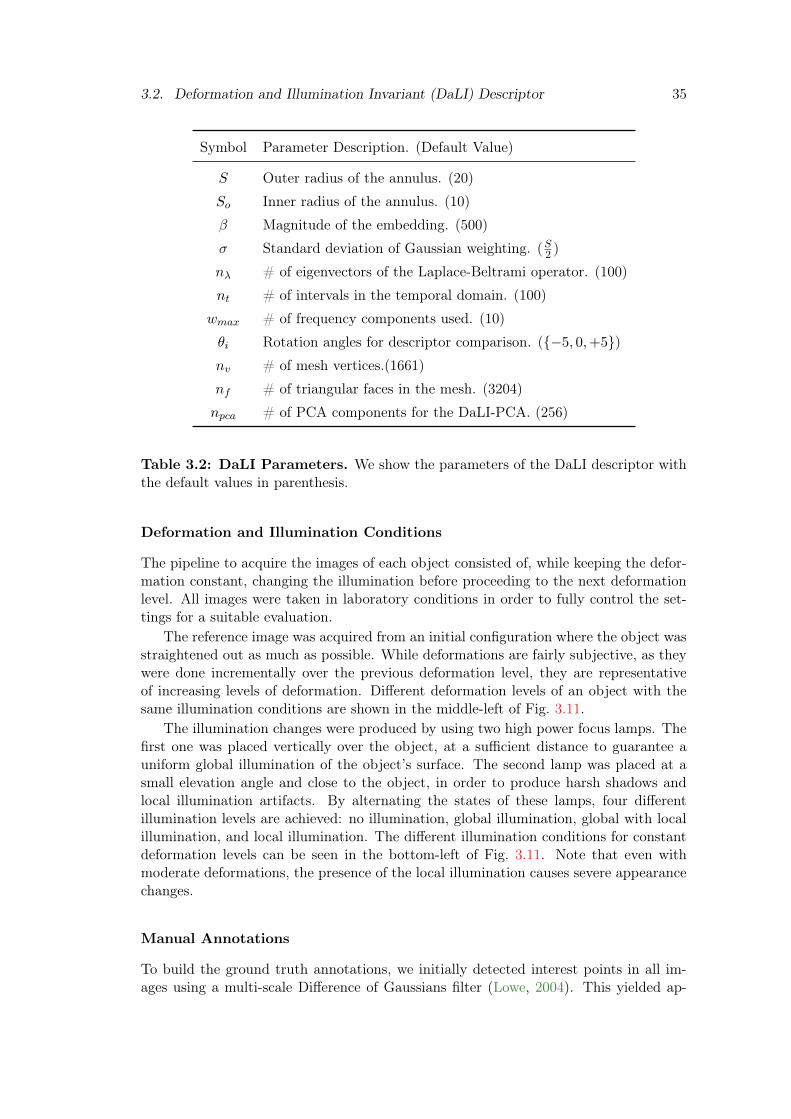
3.2. Deformation and Illumination Invariant (DaLI) Descriptor 35
Symbol Parameter Description. (Default Value)
S Outer radius of the annulus. (20)
So Inner radius of the annulus. (10)
β Magnitude of the embedding. (500)
σ Standard deviation of Gaussian weighting. (S2 )
nλ # of eigenvectors of the Laplace-Beltrami operator. (100)
nt # of intervals in the temporal domain. (100)
wmax # of frequency components used. (10)
θi Rotation angles for descriptor comparison. ({−5, 0,+5})
nv # of mesh vertices.(1661)
nf # of triangular faces in the mesh. (3204)
npca # of PCA components for the DaLI-PCA. (256)
Table 3.2: DaLI Parameters. We show the parameters of the DaLI descriptor withthe default values in parenthesis.
Deformation and Illumination Conditions
The pipeline to acquire the images of each object consisted of, while keeping the defor-mation constant, changing the illumination before proceeding to the next deformationlevel. All images were taken in laboratory conditions in order to fully control the set-tings for a suitable evaluation.
The reference image was acquired from an initial configuration where the object wasstraightened out as much as possible. While deformations are fairly subjective, as theywere done incrementally over the previous deformation level, they are representativeof increasing levels of deformation. Different deformation levels of an object with thesame illumination conditions are shown in the middle-left of Fig. 3.11.
The illumination changes were produced by using two high power focus lamps. Thefirst one was placed vertically over the object, at a sufficient distance to guarantee auniform global illumination of the object’s surface. The second lamp was placed at asmall elevation angle and close to the object, in order to produce harsh shadows andlocal illumination artifacts. By alternating the states of these lamps, four differentillumination levels are achieved: no illumination, global illumination, global with localillumination, and local illumination. The different illumination conditions for constantdeformation levels can be seen in the bottom-left of Fig. 3.11. Note that even withmoderate deformations, the presence of the local illumination causes severe appearancechanges.
Manual Annotations
To build the ground truth annotations, we initially detected interest points in all im-ages using a multi-scale Difference of Gaussians filter (Lowe, 2004). This yielded ap-
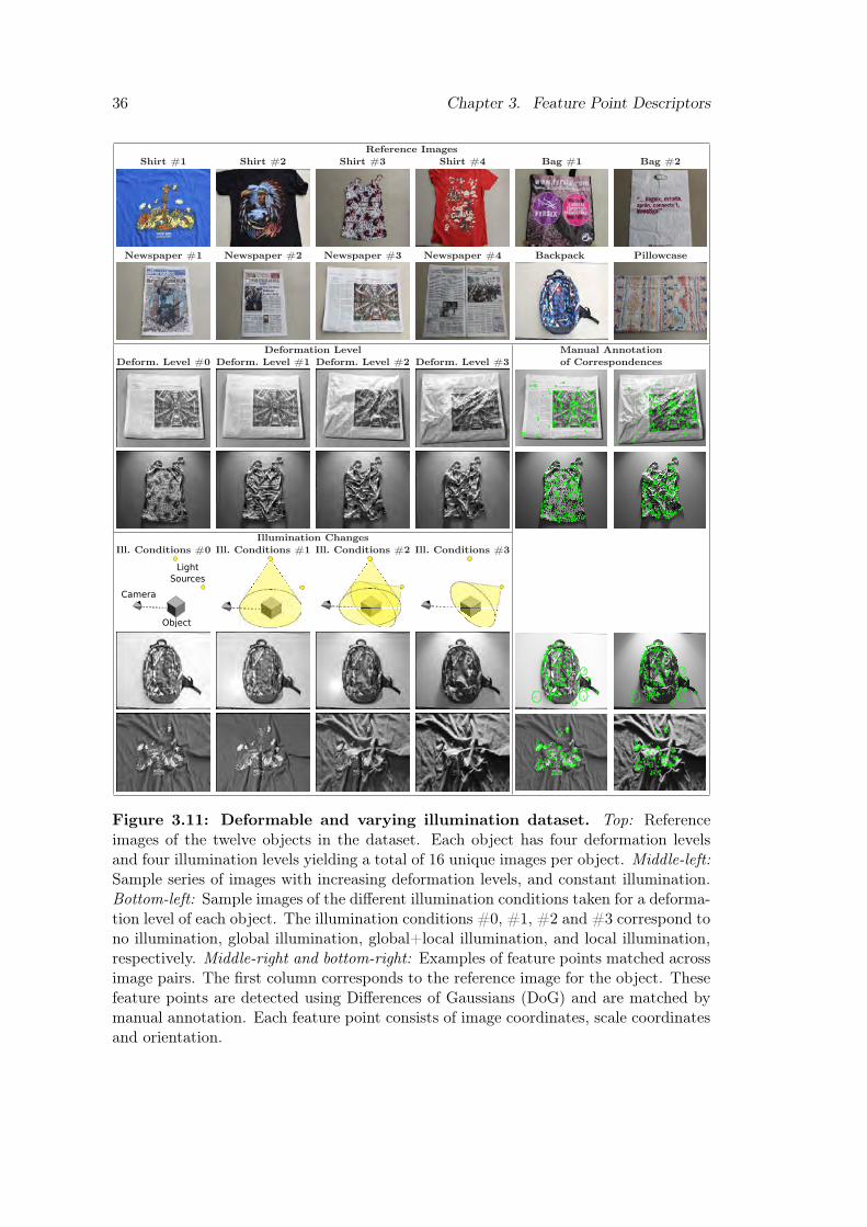
36 Chapter 3. Feature Point Descriptors
Reference Images
Shirt #1 Shirt #2 Shirt #3 Shirt #4 Bag #1 Bag #2
Newspaper #1 Newspaper #2 Newspaper #3 Newspaper #4 Backpack Pillowcase
Deformation Level Manual Annotation
Deform. Level #0 Deform. Level #1 Deform. Level #2 Deform. Level #3 of Correspondences
Illumination Changes
Ill. Conditions #0 Ill. Conditions #1 Ill. Conditions #2 Ill. Conditions #3
Light
Sources
Camera
Object
Figure 3.11: Deformable and varying illumination dataset. Top: Referenceimages of the twelve objects in the dataset. Each object has four deformation levelsand four illumination levels yielding a total of 16 unique images per object. Middle-left:Sample series of images with increasing deformation levels, and constant illumination.Bottom-left: Sample images of the different illumination conditions taken for a deforma-tion level of each object. The illumination conditions #0, #1, #2 and #3 correspond tono illumination, global illumination, global+local illumination, and local illumination,respectively. Middle-right and bottom-right: Examples of feature points matched acrossimage pairs. The first column corresponds to the reference image for the object. Thesefeature points are detected using Differences of Gaussians (DoG) and are matched bymanual annotation. Each feature point consists of image coordinates, scale coordinatesand orientation.

3.2. Deformation and Illumination Invariant (DaLI) Descriptor 37
Original Patch Rotated Scaled Cropped
Figure 3.12: Extracting patches from points of interest. Top: Outline of theprocess used to obtain patches for evaluating image descriptors. For each feature point,we initially extract a square patch centered on the feature, and whose size is proportionalto the scale factor of the interest point. The patch is then rotated according to theorientation of the feature point, and finally scaled to a constant size and cropped tobe in a circular shape. Bottom: Sample patches from the dataset, already rotated andscaled to a constant size in order to make them rotation and scale invariant.
proximately between 500− 600 feature points per image, each consisting of a 2D imagecoordinate and its associated scale.
These feature points were then manually matched for each deformation level againstthe undeformed reference image, resulting in three pairs of matched feature points. Allmatches were done with top-light illumination conditions (Ill. Conditions #1, Fig. 3.11)to facilitate the annotation task and maximize the number of repeated features betweeneach pair of images. The matching process yielded between 100 and 200 point correspon-dences for each pair of reference and deformed images. The same feature points areused for all illumination conditions for each deformation level. The middle-right im-ages of Fig. 3.11 show a few samples of our annotation. Note that the matched pointsare generally not near the borders of the image to avoid having to clip when extractingimage patches.
As we will discuss in the experimental section, in this work we seek to compare therobustness of the DaLI and other descriptors to only deformation and light changes.Yet, although the objects in the dataset are not globally rotated, the deformations doproduce local rotations. In order to compensate for this we use the SIFT descriptoras done in (Mikolajczyk and Schmid, 2005) to compute the orientation of each featurepoint, and align all corresponding features. When a feature point has more than onedominant orientation, we consider each of them to augment the set of correspondences.
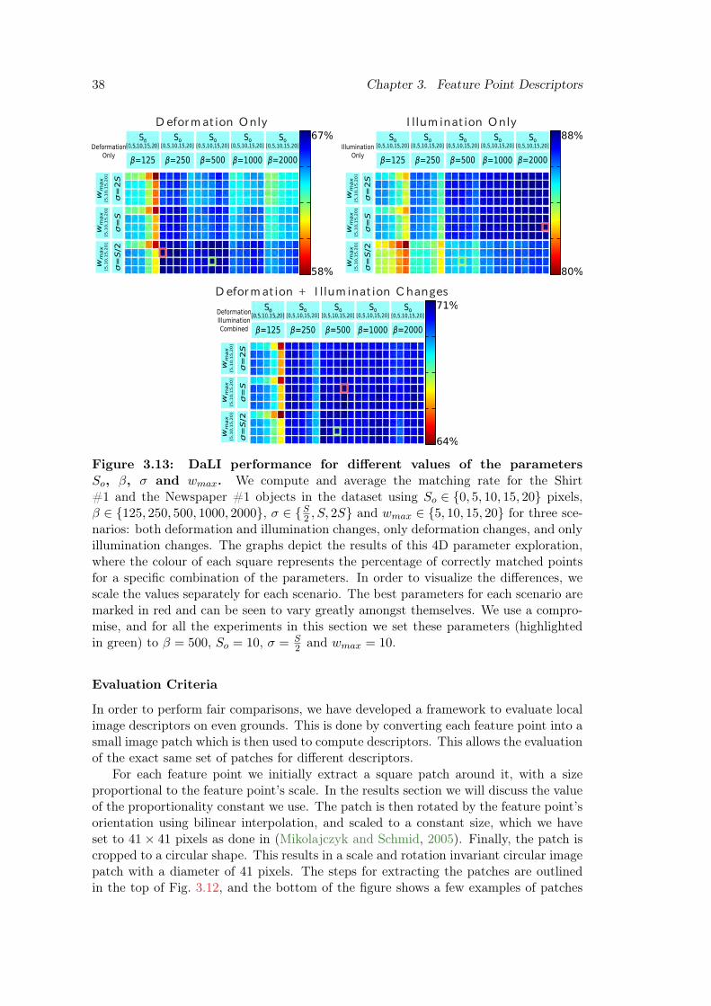
38 Chapter 3. Feature Point Descriptors
Deformat ion Only I llum inat ion Only
Deformation
Only β=125 β=250 β=500 β=1000 β=2000
σ=2S
σ=S
σ=S/2
So[0,5,10,15,20]
So[0,5,10,15,20]
So[0,5,10,15,20]
So[0,5,10,15,20]
wmax
[5,10,15,20]
wmax
[5,10,15,20]
wmax
[5,10,15,20]
67%
58%
Illumination
Only β=125 β=250 β=500 β=1000 β=2000
σ=2S
σ=S
σ=S/2
So[0,5,10,15,20]
So[0,5,10,15,20]
So[0,5,10,15,20]
So[0,5,10,15,20]
So[0,5,10,15,20]
wmax
[5,10,15,20]
wmax
[5,10,15,20]
wmax
[5,10,15,20]
88%
80%
Deformation
Illumination
Combined β=125 β=250 β=500 β=1000 β=2000
σ=2S
σ=S
σ=S/2
So[0,5,10,15,20]
So[0,5,10,15,20]
So[0,5,10,15,20]
So[0,5,10,15,20]
wmax
[5,10,15,20]
wmax
[5,10,15,20]
wmax
[5,10,15,20]
71%
64%
Deformat ion + I llum inat ion Changes
Figure 3.13: DaLI performance for different values of the parametersSo, β, σ and wmax. We compute and average the matching rate for the Shirt#1 and the Newspaper #1 objects in the dataset using So ∈ {0, 5, 10, 15, 20} pixels,β ∈ {125, 250, 500, 1000, 2000}, σ ∈ {S2 , S, 2S} and wmax ∈ {5, 10, 15, 20} for three sce-narios: both deformation and illumination changes, only deformation changes, and onlyillumination changes. The graphs depict the results of this 4D parameter exploration,where the colour of each square represents the percentage of correctly matched pointsfor a specific combination of the parameters. In order to visualize the differences, wescale the values separately for each scenario. The best parameters for each scenario aremarked in red and can be seen to vary greatly amongst themselves. We use a compro-mise, and for all the experiments in this section we set these parameters (highlightedin green) to β = 500, So = 10, σ = S
2 and wmax = 10.
Evaluation Criteria
In order to perform fair comparisons, we have developed a framework to evaluate localimage descriptors on even grounds. This is done by converting each feature point into asmall image patch which is then used to compute descriptors. This allows the evaluationof the exact same set of patches for different descriptors.
For each feature point we initially extract a square patch around it, with a sizeproportional to the feature point’s scale. In the results section we will discuss the valueof the proportionality constant we use. The patch is then rotated by the feature point’sorientation using bilinear interpolation, and scaled to a constant size, which we haveset to 41× 41 pixels as done in (Mikolajczyk and Schmid, 2005). Finally, the patch iscropped to a circular shape. This results in a scale and rotation invariant circular imagepatch with a diameter of 41 pixels. The steps for extracting the patches are outlinedin the top of Fig. 3.12, and the bottom of the figure shows a few examples of patches

3.2. Deformation and Illumination Invariant (DaLI) Descriptor 39
from the dataset.Given these “normalized patches” we then assess the performance of the descriptors
as follows. For each pair of reference/deformed images, we extract the descriptors of allfeature points in both images. We then compute the L2 distance between all descriptorsfrom the reference and the deformed image. This gives a distance matrix, which isrectangular instead of square due to the creation of additional feature points whenthere are multiple dominant orientations. Patches that have different orientations butshare the same location are treated as a unique patch. As evaluation metric we use adescriptor-independent detection rate, which is defined for the n top matches as:
Detection Rate(n) =100 ·Nc(n)
N, (3.6)
where Nc(n) is the number of feature points from the reference image that have thecorrect match among the top n candidates in the deformed image, and N is the totalnumber of feature points in the reference image.
For the experimental results we will discuss in the following section, we considerthree different evaluation scenarios: deformation and illumination, only deformation,and only illumination. In the first case we compare all combinations of deformation andillumination with respect to the reference image which has no additional illumination(ill. conditions #0) and no deformation (deform. level #0). This represents a total of15 comparisons for each object. In the second case we consider only varying levels ofdeformation for each illumination condition, which yields 12 different comparisons perobject (three comparisons per illumination level). When only considering illumination,each deformation level is compared to all illumination conditions. Again, this gives riseto 12 comparisons per object (three comparisons per deformation level).
Results
We next present the experimental results, in which we discuss the following main issues:an optimization of the descriptor parameters, a PCA-based strategy for compressingthe descriptor representation, and the actual comparison of DaLI against other state-of-the-art descriptors, for matching points of interest in the proposed dataset. Finally,we analyze specific aspects such as the performance of all descriptors in terms of theirsize, the benefits of normalizing the intensity of input images, and a real application inwhich the descriptors are compared when matching points of interest in real sequencesof a deforming cloth and a bending paper.
Choosing Descriptor’s Parameters
We next study the influence and set the values of the DaLI parameters of Table 3.2. Asthe size SP of the patch is fixed, causing the descriptor radius S to be also fixed, wewill look at finding the appropriate value of other parameters, namely the magnitudeβ of the embedding, the degree σ of smoothing within the patch, the inner radius ofthe annulus So and the dimensionality wmax of the descriptor in the frequency domain.In order to find their optimal values, we used two objects in the dataset (Shirt #1 andNewspaper #1), and computed matching rates of their feature points for a wide rangeof values for each of these parameters.
It is worth to point out that the number of eigenvectors nλ of the Laplace-Beltramioperator was set to 100 in all cases. Note that this value represents a very small portion

40 Chapter 3. Feature Point Descriptors
PCA 1 2 3 4 5 6 7 8 9 10 11 12 13 14 15 16 17 18 19 20
w = 0
w = 1
w = 2
w = 3
w = 4
w = 5
w = 6
Figure 3.14: The first 7 frequencies of the first 20 components of the PCAbasis. These are computed from images of two objects from the dataset (Shirt #1and Newspaper #1). Each vector is normalized for visualization purposes. Positivevalues are displayed in green while negative values are displayed in blue. Most of thecomponents do not contain much information at frequencies w > 6 and thus they arenot displayed, although they are considered in the DaLI-PCA descriptor.
of all potential eigenvectors, in the order of two thousands (equal to the number ofvertices nv). Using a lesser number of them would eventually deteriorate the results,while not providing a significant gain in efficiency, and using more of them, almostdid not improve the performance. Similarly, the number nt of intervals in which thetemporal domain is split is set to 100. Again, this parameter had almost no influence,neither in the performance of the descriptor nor in its computation time.
Figure 3.13 depicts the results of the parameter sweeping experiment. We display therates for three scenarios: when considering both deformation and illumination changes,only deformation changes, and only illumination changes. The most influential param-eters are the weighting factor σ and to a lesser extent the magnitude of the embeddingβ. We see that for a wide range of parameters, the results obtained are very similarwhen considering both illumination and deformation, however, there is a balance tobe struck between both deformation and illumination invariance. By increasing defor-mation invariance, illumination invariance is reduced and vice-versa. Finally we use acompromise, and the parameters we choose for all the rest of experiments are β = 500,So = 10, σ = S
2 and wmax = 10, besides the nλ = 100 and nt = 100 we mentionedearlier.
Compression with PCA
The DaLI descriptor has the downside of having a very high dimensionality, as its size isproportional to the product of the number of vertices nv used to represent the patch andthe number of frequency components wmax. For instance, using patches with a diameterof 41 pixels and considering the first 10 frequency slices, results in a 13,450-dimensionaldescriptor (1345 pixels by 10 frequency slices), requiring thus large amounts of memoryand yielding slow comparisons. However, since the descriptor is largely redundant, itcan be compacted using dimensionality reduction techniques such as (C. Strecha andFua, 2012; Cai et al., 2011; Philbin et al., 2010).
As a simple proof of concept, we have used Principal Component Analysis for

3.2. Deformation and Illumination Invariant (DaLI) Descriptor 41
100 200 300 400 500 600 700 800 900 10000.65
0.7
0.75
0.8
0.85
Dimension
Pre
cis
ion
Def.+Ill.
Illumination
Deformation
Mean
w = 0 w = 1 w = 2 w = 3 w = 4 w = 5 w = 6
DaLI
PC
AD
iff.
Figure 3.15: PCA approximation of the DaLI descriptor. Top: DaLI-PCAperformance for different compression levels. Note that the overall mean precision doesnot vary much for npca > 256 components. Bottom: Comparison of an original DaLIdescriptor with its compressed DaLI-PCA version obtained using 256 PCA components.For visualization purposes the values are normalized and the difference shown in thethird row is scaled by 5×.
performing such compression. The PCA covariance matrix is estimated on 10,436DaLI descriptors extracted from images of the Shirt #1 and Newspaper #1. Thenpca ≪ nv · wmax largest eigenvectors are then used for compressing an incoming full-size DaLI descriptor. The resulting compacted descriptor, which we call DaLI-PCA, canbe efficiently compared with other descriptors using the Euclidean distance. Fig. 3.14shows the first 7 frequencies of the first 20 vectors of the PCA-basis. It is interestingto note that most of the information can be seen to be in the lower frequencies. Thiscan be considered an experimental justification for the frequency cut off applied withthe wmax parameter, which we have previously set to 10.
In order to choose the appropriate dimension npca of the PCA-basis, we have usedour dataset to evaluate the matching rate of DaLI-PCA descriptors for different com-pression levels. The results are summarized in Fig. 3.15-top, and show that usingfewer dimensions favors deformation invariance (actually, PCA can be understood asa smoothing that undoes some of the harm of deformations) while using more dimen-sions favors illumination invariance. The response to joint deformation and illuminationchanges does not improve after using between 200−300 components, and this has beenthe criterion we used to set npca = 256 for the rest of the experiments in this section.In Fig. 3.15-bottom we compare the frequency slices for an arbitrary DaLI descriptorand its approximation with 256 PCA-modes. Observe that the differences are almostnegligible.
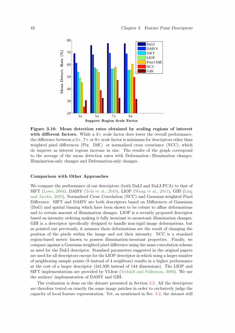
42 Chapter 3. Feature Point Descriptors
Mean
Dete
ct.
Rate
(%)
3x 5x 7x 9x20
30
40
50
60
70
80
DaLI
DAISY
SIFT
LIOP
Pixel Diff.
NCC
GIH
Support Region Scale Factor
Figure 3.16: Mean detection rates obtained by scaling regions of interestwith different factors. While a 3× scale factor does lower the overall performance,the difference between a 5×, 7× or 9× scale factor is minimum for descriptors other thanweighted pixel differences (Pix. Diff.) or normalized cross covariance (NCC), whichdo improve as interest regions increase in size. The results of the graph correspondto the average of the mean detection rates with Deformation+Illumination changes,Illumination-only changes and Deformation-only changes.
Comparison with Other Approaches
We compare the performance of our descriptors (both DaLI and DaLI-PCA) to that ofSIFT (Lowe, 2004), DAISY (Tola et al., 2010), LIOP (Wang et al., 2011), GIH (Lingand Jacobs, 2005), Normalized Cross Correlation (NCC) and Gaussian-weighted PixelDifference. SIFT and DAISY are both descriptors based on Differences of Gaussians(DoG) and spatial binning which have been shown to be robust to affine deformationsand to certain amount of illumination changes. LIOP is a recently proposed descriptorbased on intensity ordering making it fully invariant to monotonic illumination changes.GIH is a descriptor specifically designed to handle non-rigid image deformations, butas pointed out previously, it assumes these deformations are the result of changing theposition of the pixels within the image and not their intensity. NCC is a standardregion-based metric known to possess illumination-invariant properties. Finally, wecompare against a Gaussian-weighted pixel difference using the same convolution schemeas used for the DaLI descriptor. Standard parameters suggested in the original papersare used for all descriptors except for the LIOP descriptor in which using a larger numberof neighboring sample points (8 instead of 4 neighbors) results in a higher performanceat the cost of a larger descriptor (241,920 instead of 144 dimensions). The LIOP andSIFT implementations are provided by VLfeat (Vedaldi and Fulkerson, 2008). We usethe authors’ implementation of DAISY and GIH.
The evaluation is done on the dataset presented in Section 3.2. All the descriptorsare therefore tested on exactly the same image patches in order to exclusively judge thecapacity of local feature representation. Yet, as mentioned in Sec. 3.2, the dataset still

3.2. Deformation and Illumination Invariant (DaLI) Descriptor 43
Ill. Conditions #0 Ill. Conditions #1 Ill. Conditions #2 Ill. Conditions #3
Defo
rm
.Level#
0
DaLI−PCA
DaLI
DAISY
SIFT
LIOP
Pixel Diff.
NCC
GIH
Mean
Dete
ct.
Rate
(%)
2 4 6 8 100
50
100
n
Mean
Dete
ct.
Rate
(%)
2 4 6 8 100
50
100
n
Mean
Dete
ct.
Rate
(%)
2 4 6 8 100
50
100
n
Defo
rm
.Level#
1
Mean
Dete
ct.
Rate
(%)
2 4 6 8 100
50
100
n
Mean
Dete
ct.
Rate
(%)
2 4 6 8 100
50
100
n
Mean
Dete
ct.
Rate
(%)
2 4 6 8 100
50
100
n
Mean
Dete
ct.
Rate
(%)
2 4 6 8 100
50
100
n
Defo
rm
.Level#
2
Mean
Dete
ct.
Rate
(%)
2 4 6 8 100
50
100
n
Mean
Dete
ct.
Rate
(%)
2 4 6 8 100
50
100
n
Mean
Dete
ct.
Rate
(%)
2 4 6 8 100
50
100
nM
ean
Dete
ct.
Rate
(%)
2 4 6 8 100
50
100
n
Defo
rm
.Level#
3
Mean
Dete
ct.
Rate
(%)
2 4 6 8 100
50
100
n
Mean
Dete
ct.
Rate
(%)
2 4 6 8 100
50
100
n
Mean
Dete
ct.
Rate
(%)
2 4 6 8 100
50
100
n
Mean
Dete
ct.
Rate
(%)
2 4 6 8 100
50
100
n
Figure 3.17: Detection rate when simultaneously varying deformation leveland illumination conditions. Each graph represents the average of the mean detec-tion rate between the reference image (ill. conditions #0 and deform. level #0) and allimages in the dataset under specific light and deformation conditions.
requires setting the scale factor to use for the points of interest. This value correspondsto the relative size of each image patch with respect to the scale value obtained fromthe DoG feature point detector. For this purpose, we evaluated the response of alldescriptors for scale factors of 3×, 5×, 7× and 9×. The results are shown in Fig. 3.16.Although the SIFT implementation uses a default value of 3×, we have observed thatthe performance of all descriptors improves by increasing the patch size. Note that thisdoes not result in a higher computational cost, as the final size of the patch is normalizedto a circular shape with a diameter of 41 pixels. The maximum global response for all

44 Chapter 3. Feature Point Descriptors
Deform. Level #1 Deform. Level#2 Deform. Level #3
Defo
rm
ation-o
nly
DaLI−PCA
DaLI
DAISY
SIFT
LIOP
Pixel Diff.
NCC
GIH
Mean
Dete
ct.
Rate
(%)
2 4 6 8 100
50
100
n
Mean
Dete
ct.
Rate
(%)
2 4 6 8 100
50
100
n
Mean
Dete
ct.
Rate
(%)
2 4 6 8 100
50
100
n
Ill. Conditions #1 Ill. Conditions #2 Ill. Conditions #3
Illu
min
ation-o
nly
DaLI−PCA
DaLI
DAISY
SIFT
LIOP
Pixel Diff.
NCC
GIH
Mean
Dete
ct.
Rate
(%)
2 4 6 8 100
50
100
n
Mean
Dete
ct.
Rate
(%)
2 4 6 8 100
50
100
n
Mean
Dete
ct.
Rate
(%)
2 4 6 8 100
50
100
n
Figure 3.18: DaLI descriptor results for varying only deformation or illumi-nation. Top: Results when varying only the deformation while keeping the illuminationconditions constant. It can be seen that both DaLI and DAISY largely outperformthe rest of descriptors. Bottom: Results of varying only the illumination conditionswhile keeping the deformation level constant. Note that only DaLI remains robustto illumination changes. The performance of DAISY falls roughly a 20% compared toDaLI.
descriptors is achieved when using a 7× scale factor, which is the value we use for allthe experiments reported below.
The results for concurrent deformation and illumination are summarized in Fig. 3.17.DaLI consistently outperforms all other descriptors, although the more favorable re-sults are obtained under large illumination changes. The performance of DAISY isvery similar to that of DaLI when images are not affected by illumination artifacts. Inthis situation, the detection rates of DAISY are approximately between 2 − 5% belowto those obtained by DaLI. However, when illumination artifacts become more severe,the performance of DAISY rapidly drops, yielding detection rates which are more than20% below DaLI. SIFT, LIOP, and Pixel Difference yield similar results, with SIFTbeing better at weak illumination changes and LIOP better at handling strong illu-mination changes. Yet, these three methods are one step behind DaLI and DAISY.NCC generally performs worse except in situations with large illumination changes,where it even outperforms DAISY. On the other hand, GIH performs quite poorly evenwhen no light changes are considered. This reveals another limitation of this approach,in that it assumes the effect of deformations is to locally change the position of imagepixels, while in real deformations some of the pixels may disappear due to occlusions.Although our approach does not explicitly address occlusions, we can partially handle

3.2. Deformation and Illumination Invariant (DaLI) Descriptor 45
Reference Image SIFT DAISY LIOP GIH DaLI
n=10n 10
n=9
=8
n=7
n=8
=8
n=6
n=5
n=4
n=3
n=2
n=1
Figure 3.19: Sample results from the dataset. As in Fig. 3.2, the colour of thecircles indicates the position n of the correct match among the top candidates. If n > 10we consider the point as unmatched and mark it with a cross.
them by weighing the contribution of the pixels within each patch, by a function de-creasing with the distance to the center. Thus, most of the information of our descriptoris concentrated in a small region surrounding the point of interest, hence making it lesssensitive to occlusions. The results also show that the compressed DaLI-PCA followsa similar pattern as DaLI, and specially outperforms DAISY under severe illuminationconditions.
In Fig. 3.18 we give stronger support to our arguments by independently evaluatingdeformations and illumination changes. These graphs confirm that under deformation-only changes, DaLI outperforms DaLI-PCA and DAISY by a small margin of roughly3%. Next, SIFT, LIOP, and Pixel Difference yield similar results, roughly 20% belowDaLI in absolute terms. GIH and NCC yield also similar results, although their per-formance is generally very poor. When only illumination changes are considered, bothDaLI and DaLI-PCA significantly outperform other descriptors, by a margin larger than20% when dealing with complex illumination artifacts. The only notable difference inthis scenario is that the NCC descriptor outperforms SIFT and Pixel Difference. AsGIH is not invariant to illumination changes, it obtains poor results. Similarly, sinceLIOP is designed to be invariant to monotonic lighting changes, it does not performthat well in real images that undergo complex illumination artifacts.
In summary, the experiments have shown that DaLI globally obtains the best per-formance. Its best relative response when compared with other descriptors is obtainedwhen the deformations are mild and the light changes drastic. Some sample results onparticular images taken from the dataset can be seen in Fig. 3.19. Additionally, nu-meric results for the best candidate (n = 1 in Eq. 3.6) under different conditions for all

46 Chapter 3. Feature Point Descriptors
Descriptor Deformation Illumination Deformation+Illumination
DaLI-PCA 67.425 85.122 68.368
DaLI 70.577 89.895 72.912
DAISY 67.373 75.402 66.197
SIFT 55.822 60.760 53.431
LIOP 58.763 60.014 52.176
Pixel Diff. 54.714 65.610 54.382
NCC 38.643 62.042 41.998
GIH 37.459 28.556 31.230
Table 3.3: Evaluation results on the dataset for all descriptors. Results areobtained by averaging the first match percentage values over all images being testedunder all different conditions.
True Positive Pairs False Positive Pairs
False Negative Pairs True Negative Pairs
Figure 3.20: True positive, false positive, false negative and true negativeimage patch pairs. These were obtained using the DaLI descriptor on the dataset.Note that most of the false negatives are due to large orientation changes across featurepoints.
descriptors are shown in Table 3.3.
Finally, examples of particular patch matches are depicted in Fig. 3.20. The truepositives pairs can be seen to be matched despite large changes. On the other hand,the false negatives seem largely generated by differences in orientations of the featurepoints: they correspond to the same patch, only rotated. The false positives share somesimilarity, although they are mainly from heavily deformed images.
Descriptor Size Performance
Since larger descriptors may a priori have an unfair advantage, we next provide resultsof an additional experiment in which we compare descriptors having similar sizes. TheLIOP we calculate in this case uses 4 neighbours instead of the 8 neighbours we consid-ered before, which results in a smaller size, although also in a lower performance. GIH

3.2. Deformation and Illumination Invariant (DaLI) Descriptor 47
Deforming Cloth
20 40 60 80 100 120 140 16020
40
60
80
100
Me
an
De
tect.
Ra
te (
%)
Frame
DaLI
DAISY
SIFT
Paper Bending
20 40 60 80 100 120 140 16020
40
60
80
100
Mean D
ete
ct. R
ate
(%
)
Frame
DaLI
DAISY
SIFT
Figure 3.21: Mean detection accuracy on two real world videosfrom (Moreno-Noguer and Fua, 2013). For each sequence we show three ex-ample frames from each video in the top row. In the bottom row we plot the accuracyfor each frame for three descriptors: DaLI, DAISY and SIFT. Additionally the meanfor each descriptor is displayed as a dashed line.
is originally 176-dimensional, thus the results are the same as in Table 3.3. NCC andPixel Diff, are not considered for this experiment as their size is 41× 41 = 1681.
Results are shown in Table 3.4. We can see that the 128-dimensional DaLI-PCAoutperforms all other descriptors except the 256-dimensional DaLI-PCA. It is worth

48 Chapter 3. Feature Point Descriptors
Descriptor Size Deformation Illumination Deformation+Illumination
DaLI-PCA 128 67.45 82.34 67.71
SIFT 128 55.82 60.76 53.43
LIOP 144 54.01 44.89 44.45
DAISY 200 67.37 75.40 66.20
GIH 176 37.46 28.56 31.23
DaLI-PCA 256 67.43 85.12 68.37
Table 3.4: Comparison of performance and descriptor size.
noting the large performance gain obtained over the standard SIFT descriptor.
Effects of Intensity Normalization
We next extend the analysis we introduced in Sect. 3.2 in which we evaluated SI-HKSand HKS with and without pre-normalizing the intensity of input images. We willalso consider SIFT and DAISY, which have been the most competitive descriptors inprevious experiments. Since SIFT/DAISY implementations require the pixels to bein a [0, 1] range, we have normalized each image patch so that the pixels follow thedistribution N (0.5, (2 · 1.956)−1). This makes it so that on average 95% of the pixelswill fall in [0, 1]. Pixels outside of this range are set to either 0 or 1.
We compare the DaLI descriptor (both its SI-HKS and HKS variants), DAISY andSIFT, with and without normalization. Results are shown in Table 3.5. We can seethat for DAISY and SIFT, since they perform a final normalization stage, the results donot have any significant change. In the case of the DaLI descriptor, though, we observethat there is a rather significant performance increase when using the SI-HKS variantover the HKS one, even with patch normalization. This demonstrates again that therole of the Fourier Transforms applied in HKS to make it illumination invariant go farbeyond a simple normalization. In addition, SI-HKS compresses the descriptor in thefrequency domain and is one order of magnitude smaller than the HKS variant.
Evaluation on Real World Sequences
This section describes additional experiments on two real world sequences of deformingobjects, taken from (Moreno-Noguer and Fua, 2013). One consists of a T-Shirt beingwaved in front of a camera (Deforming Cloth) and the other consists of a piece of paperbeing bended in front of a camera (Paper Bending). We use points of interest computedwith the Differences of Gaussians detector (DoG) and follow the same patch extractionapproach as in the rest of the paper. The points of interest are calculated for the firstframe in each sequence and then propagated using the provided 3D ground truth to theother frames. We use the same descriptor parameters as in the rest of the experiments,and seek to independently match the points of interest in the first frame to those of allthe other frames.

3.3. Deep Architectures for Descriptors 49
Descriptor Normalization? Deformation IlluminationDeformation+Illumination
DaLI (SI-HKS) No 70.58 89.90 72.91
DaLI (SI-HKS) Yes 70.38 88.60 72.28
DaLI (HKS) No 66.27 84.21 67.83
DaLI (HKS) Yes 67.20 84.62 69.42
DAISY No 67.37 75.40 66.20
DAISY Yes 67.08 75.59 66.27
SIFT No 55.82 60.76 53.43
SIFT Yes 55.05 61.83 53.21
Table 3.5: Effect of normalizing image patches for various descriptors.
As we can observe in Fig. 3.21, DaLI outperforms both DAISY and SIFT2 . Weobtain a 5.5% improvement over DAISY on the Deforming Cloth sequence and a 4.1%improvement on the Paper Bending sequence. Note that these sequences do not haveas complicated illumination artifacts as our dataset, an unfavorable situation for ourdescriptor. Yet, DaLI still consistently outperforms other approaches along the wholesequence.
3.3 Deep Architectures for Descriptors
While most descriptors use hand-crafted features (Lowe, 2004; Bay et al., 2006; Kokkinoset al., 2012; Trulls et al., 2013), including the DaLI descriptor (Simo-Serra et al., 2015b)presented in the previous section, there has recently been interest in using machinelearning algorithms to learn descriptors from large databases.
In this section we draw inspiration on the recent success of Deep ConvolutionalNeural Networks on large-scale image classification problems (Krizhevsky et al., 2012;Szegedy et al., 2013) to build discriminative descriptors for local patches. Specifically,we propose an architecture based on a Siamese structure of two CNNs that share theparameters. We compute the L2 norm on their output, i.e. the descriptors, and use aloss that enforces the norm to be small for corresponding patches and large otherwise.We demonstrate that this approach allows us to learn compact and discriminative rep-resentations.
To implement this approach we rely on the dataset of (Brown et al., 2011), whichcontains over 1.5M grayscale 64×64 image patches from different views of 500K different3D points. With such large datasets it becomes intractable to exhaustively exploreall corresponding and non-corresponding pairs. Random sampling is typically used;however, most correspondences are not useful and hinder the learning of a discriminantmapping. We address this issue with aggressive mining of “hard" positives and negativesand which proves fundamental in order to obtain discriminative learned descriptors. In
2Again, we only compare against DAISY and SIFT, as these are the descriptors which have beenmore competitive in the experiments with the full dataset.

50 Chapter 3. Feature Point Descriptors
particular, in some of the tests we obtain up to a 169% increase in performance withSIFT as a baseline.
Related Work
Recent developments in the design of local image descriptors are moving from carefully-engineered features (Lowe, 2004; Bay et al., 2006) to learning features from large volumesof data. This line of works includes unsupervised techniques based on hashing as wellas supervised approaches using Linear Discriminant Analysis (Brown et al., 2011; Gonget al., 2012; C. Strecha and Fua, 2012), boosting (Trzcinski et al., 2012), and convexoptimization (Simonyan et al., 2014).
We explore solutions based on deep convolutional networks (CNNs). CNNs havebeen used in computer vision for decades, but are currenly experiencing a resurgencekickstarted by the accomplishments of (Krizhevsky et al., 2012) on large-scale imageclassification. The application of CNNs to the problem of descriptor learning has al-ready been explored by some researchers (Jahrer et al., 2008; Osendorfer et al., 2013).These works are however preliminary, and many open questions remain regarding thepractical application of CNNs for learning descriptors, such as the most adequate net-work architectures and application-dependent training schemes. We aim to providea rigorous analysis of several of these topics. In particular, we use a Siamese net-work (Bromley et al., 1994) to train the models, and experiment with different networkconfigurations inspired by the state-of-the-art in deep learning.
Additionally, we demonstrate that aggressive mining of both “hard” positive and neg-ative matching pairs greatly enhances the learning process. Mining hard negatives isa well-known procedure in sliding-window detectors (Felzenszwalb et al., 2010), wherethe number of negative samples is virtually unlimited and yet most negatives are easilydiscriminated. Similar techniques have been applied to CNNs for object detection (Gir-shick et al., 2014; Szegedy et al., 2013).
Learning Deep Descriptors
Given an intensity patch x ∈ RN , the descriptor of x is a non-linear mapping D(x)
that is expected to be discriminative, i.e. descriptors for image patches correspondingto the same point should be similar, and dissimilar otherwise.
In the context of multiple-view geometry, descriptors are typically computed forsalient points where scale and orientation can be reliably estimated, for invariance.Patches then capture local projections of 3D scenes. Let us consider that each imagepatch xi has an index pi that uniquely identifies the 3D point which roughly projectsonto the 2D patch, from a specific viewpoint. Therefore, taking the L2 norm as asimilarity metric between descriptors, for an ideal descriptor we would wish that
dD(x1,x2) = ‖D(x1)−D(x2)‖2 =
{
0 if p1 = p2
∞ if p1 6= p2. (3.7)
We propose learning descriptors using a Siamese network (Bromley et al., 1994),i.e. optimizing the model for pairs of corresponding or non-corresponding patches,as shown in Fig. 3.22a. We propagate the patches through the model to extract thedescriptors and compute their L2 norm, which is a standard similarity measure for

3.3. Deep Architectures for Descriptors 51
(a) Siamese network.
Name Layer 1 Layer 2 Layer 3 Layer 4
CNN3_NN132x7x7 64x6x6 128x5x5 128
x2 pool x3 pool x4 pool -
CNN332x7x7 64x6x6 128x5x5 -
x2 pool x3 pool x4 pool -
CNN2a_NN132x5x5 64x5x5 128 -
x3 pool x4 pool - -
CNN2b_NN132x9x9 64x5x5 128 -
x4 pool x5 pool - -
CNN264x5x5 128x5x5 - -
x4 pool x11 pool - -
CNN1_NN132x9x9 128 - -
x14 pool - - -
(b) Various convolutional neural network architectures.
Figure 3.22: Overview of the network architectures used. Left: Schematic of aSiamese network, where pairs of input patches are processed by two copies of the sameCNN. Right: Different CNN configurations considered.
image descriptors. We then compute the loss function on this distance. Given a pair ofpatches x1 and x2 we define a loss function of the form
l(x1,x2, δ) = δ · lP (dD(x1,x2)) + (1− δ) · lN (dD(x1,x2)) , (3.8)
where δ is the indicator function, which is 1 if p1 = p2, and 0 otherwise. lP and lNare the partial loss functions for patches corresponding to the same 3D point and todifferent points, respectively. When performing back-propagation, the gradients areindependently accumulated for both descriptors, but jointly applied to the weights, asthey are shared.
Although it would be ideal to optimize directly for Eq. (3.7), we relax it, using amargin m for lN (·). In particular, we consider the hinge embedding criterion (Mobahiet al., 2009)
lP (dD(x1,x2)) = dD(x1,x2) (3.9)
lN (dD(x1,x2)) = max(0,m− dD(x1,x2)) . (3.10)
Convolutional Neural Network Descriptors
When designing the structure of the CNN we are limited by the size of the input data,in our case 64×64 patches from the dataset of (Brown et al., 2011). Note that largerpatches would allow us to consider deeper networks, and possibly more informative de-scriptors, but at the same time they would be also more susceptible to occlusions. Weconsider networks of up to three convolutional layers, followed by up to a single addi-tional fully-connected layer. We target descriptors of size 128, the same as SIFT (Lowe,2004); this value also constrains the architectures we can explore.

52 Chapter 3. Feature Point Descriptors
As usual, each convolutional layer consists four sub-layers: filter layer, non-linearitylayer, pooling layer and normalization layer. Since sparser connectivity has been shownto improve performance while lowering parameters and increasing speed (Culurcielloet al., 2013), except for the first layer, the filters are not densely connected to theprevious layers. Instead, they are sparsely connected at random, so that the meannumber of connections each input layer has is constant.
Regarding the non-linear layer, we use hyperbolic tangent (Tanh), as we found itperforms better than Rectified Linear Units (ReLU). We use L2 pooling for the poolingsublayers, which were shown to outperfom the more standard max pooling (Sermanetet al., 2012). Normalization has been shown to be important for deep networks (Jarrettet al., 2009) and fundamental for descriptors (Mikolajczyk and Schmid, 2005). We usesubtractive normalization for a 5×5 neighbourhood with a Gaussian kernel. We willlater justify these decisions empirically.
An overview of the architectures we consider is given in Fig. 3.22b. We choose aset of six networks, from 2 up to 4 layers. The architecture hyperparameters (numberof layers and convolutional/pooling filter size) are chosen so that no padding is needed.We consider models with a final fully-connected layer as well as fully convolutionalmodels, where the last sublayer is a pooling layer. Our implementation is based onTorch7 (Collobert et al., 2011).
Stochastic Sampling Strategy and Mining
Our goal is to optimize the network parameters from an arbitrarily large set of trainingpatches. Let us consider a dataset with N patches and M ≤ N unique 3D patch indices,each with ni associated image patches. Then, the number of matching image patchesor positives NP and the number of non-matching images patches or negatives NN inthe dataset is
NP =M∑
i=1
ni(ni − 1)
2and NN =
M∑
i=1
ni(N − ni) . (3.11)
In general both NP and NN are intractable to exhaustively iterate over. We approachthe problem with random sampling. For gathering positives samples we can randomlychoose a set of BP 3D point indices {p1, · · · , pBP
}, and choose two patches with corre-sponding 3D point indices randomly. For negatives it is sufficient to choose BN randompairs with non-matching indices.
However, when the pool of negative samples is very large random sampling willproduce many negatives with a very small loss, which do not contribute to the globalloss, and thus stifle the learning process. Instead, we can iterate over non-correspondingpatch pairs to search for “hard” negatives, i.e. with a high loss. In this manner itbecomes feasible to train discriminative models faster while also increasing performance.This technique is commonplace in sliding-window classification.
Therefore, at each epoch we generate a set of BN randomly chosen patch pairs,and after forward-propagation through the network and computing their loss we keeponly a subset of the BM
N “hardest” negatives, which are back-propagated through thenetwork in order to update the weights. Additionally, the same procedure can beused over the positive samples, i.e. we can sample BP corresponding patch pairs andprune them down to the BM
P “hardest” positives. We show that the combination of
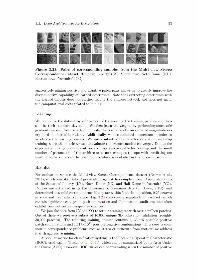
3.3. Deep Architectures for Descriptors 53
Figure 3.23: Pairs of corresponding samples from the Multi-view StereoCorrespondence dataset. Top row: ‘Liberty’ (LY). Middle row: ‘Notre Dame’ (ND).Bottom row: ‘Yosemite’ (YO).
aggressively mining positive and negative patch pairs allows us to greatly improve thediscriminative capability of learned descriptors. Note that extracting descriptors withthe learned models does not further require the Siamese network and does not incurthe computational costs related to mining.
Learning
We normalize the dataset by subtraction of the mean of the training patches and divi-sion by their standard deviation. We then learn the weights by performing stochasticgradient descent. We use a learning rate that decreases by an order of magnitude ev-ery fixed number of iterations. Additionally, we use standard momentum in order toaccelerate the learning process. We use a subset of the data for validation, and stoptraining when the metric we use to evaluate the learned models converges. Due to theexponentially large pool of positives and negatives available for training and the smallnumber of parameters of the architectures, no techniques to cope with overfitting areused. The particulars of the learning procedure are detailed in the following section.
Results
For evaluation we use the Multi-view Stereo Correspondence dataset (Brown et al.,2011), which consists of 64×64 grayscale image patches sampled from 3D reconstructionsof the Statue of Liberty (LY), Notre Dame (ND) and Half Dome in Yosemite (YO).Patches are extracted using the Difference of Gaussians detector (Lowe, 2004), anddetermined as a valid correspondence if they are within 5 pixels in position, 0.25 octavesin scale and π/8 radians in angle. Fig. 3.23 shows some samples from each set, whichcontain significant changes in position, rotation and illumination conditions, and oftenexhibit very noticeable perspective changes.
We join the data from LY and YO to form a training set with over a million patches.Out of these we reserve a subset of 10,000 unique 3D points for validation (roughly30,000 patches). The resulting training dataset contains 1,133,525 possible positivepatch combinations and 1.117×10¹² possible negative combinations. This skew is com-mon in correspondence problems such as stereo or structure from motion; we addressit with aggressive mining.
A popular metric for classification systems is the Receiving Operator Characteristic(ROC), used e.g. in (Brown et al., 2011), which can be summarized by its Area Underthe Curve (AUC). However, ROC curves can be misleading when the number of positive

54 Chapter 3. Feature Point Descriptors
Architecture Parameters PR AUC
SIFT — 0.361
CNN1_NN1 68,352 0.032
CNN2 27,776 0.379
CNN2a_NN1 145,088 0.370
CNN2b_NN1 48,576 0.439
CNN3_NN1 62,784 0.289
CNN3 46,272 0.558
Table 3.6: Effect of network architectures. We look at the effects of networkdepth, and fully convolutional networks vs networks with a fully-connected layer. ThePR AUC is calculated on the validation set for the top-performing iteration.
Architecture PR AUC
SIFT 0.361
CNN3 0.558
CNN3 ReLU 0.442
CNN3 No Norm 0.511
CNN3 MaxPool 0.420
Table 3.7: Comparison of network hyperparameters. We compare the fullyconvolutional CNN3 architecture with different hyperparameters settings such as Tanhand ReLU rectification layers, without normalization, and with max pooling instead ofL2 pooling. The best results are obtained for Tanh units, normalization, and L2 pooling(i.e. ‘CNN3’). The PR AUC is computed on the validation set for the top-performingiteration.
and negative samples are very different (Davis and Goadrich, 2006), and is alreadynearly saturated for the baseline descriptor SIFT. A richer metric is the Precision-Recallcurve (PR). We benchmark our models with PR curves and their AUC. In particular,for each of the 10,000 unique points in the validation set we randomly sample twocorresponding patches and 1,000 non-corresponding patches, and use them to computethe PR curve. We rely on the validation set for the LY+YO split to examine differentconfigurations, network architectures and mining techniques.
Finally, we evaluate the top-performing models over the test set. We follow thesame procedure as for validation, compiling the results for 10,000 points with 1,000non-corresponding matches each, now over 10 different folds. We run three differ-ent splits, for generalization: LY+YO (tested on ND), LY+ND (tested on YO), andYO+ND (tested on LY).
We will consider all hyperparameters to be the same unless otherwise mentioned,i.e. a learning rate of 0.01 that decreases ever 10, 000 iterations by a factor of 10. Weconsider negative mining with BN = 256 and BM
N = 128, and no positive mining; i.e.BP = BM
P = 128.

3.3. Deep Architectures for Descriptors 55
Recall0 0.1 0.2 0.3 0.4 0.5 0.6 0.7 0.8 0.9 1
Pre
cis
ion
0
0.1
0.2
0.3
0.4
0.5
0.6
0.7
0.8
0.9
1PR curve, validation set
SIFTCNN1_NN1CNN2CNN2a_NN1CNN2b_NN1CNN3_NN1CNN3
Figure 3.24: Precision-recall curves for different network architectures. Welook at the effect of network depth (up to 3 CNN layers), and fully convolutionalnetworks vs networks with final fully-connected layer (NN1). Fully-convolutional modelsoutperform models with fully-connected neural network at the end.
Recall0 0.1 0.2 0.3 0.4 0.5 0.6 0.7 0.8 0.9 1
Pre
cis
ion
0
0.1
0.2
0.3
0.4
0.5
0.6
0.7
0.8
0.9
1PR curve, validation set
SIFTCNN3CNN3_ReLUCNN3_NoNormCNN3_MaxPool
Figure 3.25: Precision-recall curves for different network hyperparameters.We analyze fully convolutional CNN3 models with Tanh and ReLU, without normal-ization, and with max pooling instead of L2 pooling. The best results are obtained forTanh units, normalization, and L2 pooling (‘CNN3’ model).
Depth and Fully Convolutional Architectures
The network depth is constrained by the size of the patch. We consider only up to 3 con-volutional layers (CNN1-3). Additionally, we consider adding a single fully-connected

56 Chapter 3. Feature Point Descriptors
RP RN Cost PR AUC
1 1 — 0.366
1 2 20% 0.558
2 2 35% 0.596
4 4 48% 0.703
8 8 67% 0.746
16 16 80% 0.538
Table 3.8: Effect of mining samples on performance. Mining factors indicatethe samples considered (BP , BN ), i.e. 1: 128, 2: 256, 4: 512, 8: 1024, and 16: 2048, ofwhich 128 are used for training. Column 3 indicates the fraction of the computationalcost spent mining.
Architecture Output Parameters PR AUC
SIFT 128D — 0.361
CNN3 128D 46,272 0.596
CNN3 Wide 128D 110,496 0.552
CNN3_NN1 128D 62,784 0.456
CNN3_NN1 32D 50,400 0.389
Table 3.9: Effect of number of filters and fully-connected layer. The bestresults are obtained with fully-convolutional networks with a fewer number of filters.
layer at the end (NN1). Fully-connected layers increase the number of parameters bya large factor, which increases the difficulty of learning and can lead to overfitting. Weshow the results of the various architectures we evaluate in Table 3.6 and Fig. 3.24.Deeper networks outperform shallower ones, and architectures with a fully-connectedlayer at the end do worse than fully convolutional architectures. In the following ex-periments with consider only models with 3 convolutional layers.
Hidden Units Mapping, Normalization, and Pooling
It is generally accepted that Rectified Linear Units (ReLU) perform much better inclassification tasks (Krizhevsky et al., 2012) than other non-linear functions. They are,however, ill-suited for regression tasks (such as the problem in hand), as they can onlyoutput positive values. We consider both the standard Tanh and ReLU. For the ReLUcase we still use Tanh for the last layer. We also consider not using the normalizationsublayer for each of the convolutional layers. Finally, we consider using max poolingrather than L2 pooling. We show results for the fully-convolutional CNN3 architecturein Table 3.7 and Fig. 3.25. The best results are obtained with Tanh, normalization andL2 pooling (‘CNN3’ in the table/plot). We will use this configuration in the followingexperiments.

3.3. Deep Architectures for Descriptors 57
Recall0 0.1 0.2 0.3 0.4 0.5 0.6 0.7 0.8 0.9 1
Pre
cis
ion
0
0.1
0.2
0.3
0.4
0.5
0.6
0.7
0.8
0.9
1PR curve, validation set
SIFTCNN3, no miningCNN3, mined 1/2CNN3, mined 2/2CNN3, mined 4/4CNN3, mined 8/8CNN3, mined 16/16
Figure 3.26: Precision-recall curves for different levels of mining. The bestresults are obtained with 8/8 factors, i.e. pools of 1024 samples filtered down to 128.
Recall0 0.1 0.2 0.3 0.4 0.5 0.6 0.7 0.8 0.9 1
Pre
cis
ion
0
0.1
0.2
0.3
0.4
0.5
0.6
0.7
0.8
0.9
1PR curve, validation set
SIFTCNN3 (mined 2/2)CNN3 Wide (mined 2/2)CNN3_NN1 128D (mined 2/2)CNN3_NN1 32D (mined 2/2)
Figure 3.27: Precision-recall curves for different number of filters and fully-connected layers. We show several results for different number of filters and fully-connected layers for dimensionality reduction. The best results are obtained with fully-convolutional networks.
Mining
We analyze the effect of both positive and negative mining by training different modelsin which a large, initial pool of BP positives and BN negatives are pruned to a smallernumber of ‘hard’ positive and negative matches, used to update the parameters of thenetwork. We keep this batch size for parameter learning constant, with BM
N = 128 and

58 Chapter 3. Feature Point Descriptors
Train Test SIFTCNN3 CNN3 CNN3 CNN3 Improvement
mine-1/2 mine-2/2 mine-4/4 mine-8/8 (Best vs SIFT)
LY+YOS ND 0.349 0.535 0.555 0.630 0.667 91.1%
LY+ND YOS 0.425 0.383 0.390 0.502 0.545 28.2%
YOS+ND LY 0.226 0.460 0.483 0.564 0.608 169.0%
Table 3.10: Precision-recall area under the curve for the generalized resultsover the three dataset splits.
Recall0 0.1 0.2 0.3 0.4 0.5 0.6 0.7 0.8 0.9 1
Pre
cis
ion
0
0.1
0.2
0.3
0.4
0.5
0.6
0.7
0.8
0.9
1PR curve, training LY+YO, test ND
SIFTCNN3, mined 1/2CNN3, mined 2/2CNN3, mined 4/4CNN3, mined 8/8
Recall0 0.1 0.2 0.3 0.4 0.5 0.6 0.7 0.8 0.9 1
Pre
cis
ion
0
0.1
0.2
0.3
0.4
0.5
0.6
0.7
0.8
0.9PR curve, training LY+ND, test YO
SIFTCNN3, mined 1/2CNN3, mined 2/2CNN3, mined 4/4CNN3, mined 8/8
Recall0 0.1 0.2 0.3 0.4 0.5 0.6 0.7 0.8 0.9 1
Pre
cis
ion
0
0.1
0.2
0.3
0.4
0.5
0.6
0.7
0.8
0.9
1PR curve, training YO+ND, test LY
SIFTCNN3, mined 1/2CNN3, mined 2/2CNN3, mined 4/4CNN3, mined 8/8
Figure 3.28: Precision-recall curves for the generalized results over the threedataset splits.
BMP = 128, and increase the ratio of both negative mining RN = BN/B
MN and positive
mining RP = BP /BMP . We keep all other parameters constant. We use the notation
RP /RN , for brevity.
Large mining factors have a high computational cost, up to 80% of the total com-putational cost, which includes mining (i.e. forward propagation of all BP and BNsamples) and learning (i.e. backpropagating the “hard” positive and negative samples).In order to speed up the learning process we initialize the CNN3 models with positivemining, i.e. 2/2, 4/4, 8/8 and 16/16, with an early iteration of a model trained onlywith negative mining (1/2).
Results are shown in Table 3.8 and Fig. 3.26. We see that for this particular problemaggressive mining is fundamental. This is likely due to the extremely large numberof both negatives and positives in the dataset, in combination with models with a lownumber of parameters. We observe a drastic increase in performance up to 8/8 miningfactors.
Number of Filters and Descriptor Dimension
We analyze increasing the number of filters in the CNN3 model, and adding a fully-connected layer that can be used to decrease the dimensionality of the descriptor. Weconsider increasing the number of filters in layers 1 and 2 from 32 and 64 to 64 and96, respectively. Additionally, we double the number of internal connections betweenlayers. This more than doubles the number of parameters in this network. To analyzedescriptor dimensions we consider the CNN3_NN1 model and change the number ofoutputs in the last fully-connected layer from 128 to 32. In this case we consider posi-tive mining with BP = 256 (i.e. 2/2). Results can be seen in Table 3.9 and Fig. 3.27.
3.4. Summary 59
The best results are obtained with fewer filters and fully-convolutional networks. Addi-tionally we notice that mining is also instrumental for models the NN1 layer (compareresults with Table 3.6).
Generalization
In this section we consider the three dataset splits. We train the best performingmodels, i.e. CNN3 with different mining ratios, on a combination of two sets, andtest them on the remaining set. We select the training iteration that performs bestover the validation set. The test datasets are very large (up to 633K patches) andwe use the same procedure as for validation, evaluating 10,000 unique points, eachwith 1,000 random non-corresponding matches. We repeat this process over 10 folds,thus considering 100,000 sets of one corresponding patch vs 1,000 non-correspondingpatches. We show results in terms of PR AUC in Table 3.10, and the correspondingPR curves are pictured in Fig. 3.28.
We report consistent improvements over the baseline, i.e. SIFT. The performancevaries significantly from split to split; this is due to the nature of the different sets.‘Yosemite’ contains mostly fronto-parallel translations with illumination changes and noocclusions (Fig. 3.23, row 3); SIFT performs well on this data. Our learned descriptorsoutperform SIFT on the high-recall regime (over 20% of the samples; see Fig. 3.28),and is 28% better overall in terms of PR AUC. The effect is much more dramatic on‘Notredame’ and ‘Liberty’, which contains significant patch translation and rotation,as well as viewpoint changes around outcropping non-convex objects which result inocclusions (see Fig. 3.23, rows 1-2). Our learned descriptors outperform SIFT by 91%and 169% testing over ND and LY, respectively.
Qualitative analysis
Fig. 3.29 shows samples of matches retrieved with our CNN3-mined-4/4 network, overthe validation set for the first split. In this experiment the corresponding patches wereranked in the first position in 76.5% of cases; a remarkable result, considering that everytrue match had to be chosen from a pool of 1,000 false correspondences. The right-handimage shows cases where the ground truth match was not ranked first; notice thatmost of these patches exhibit significant changes of appearance. We include a failurecase (highlighted in red), caused by a combination of large viewpoint and illuminationchanges; however, these misdetections are very uncommon.
3.4 Summary
In this chapter we have presented two vastly different approaches at tackling the sameproblem: discriminative representation of local image patches, i.e., feature point descrip-tors. Our first approach is more traditional in the sense it is a hand-crafted descriptor forthe specific problem of deformation and illumination invariant feature point descriptors.For our second approach we propose a data-driven approach in which given enough datawe are able to learn the descriptor. Both approaches are complementary and can beused in a variety of different applications.
On one hand, heat diffusion theory has been recently shown effective for 3D shaperecognition tasks. We have proposed using these techniques to build DaLI, a feature
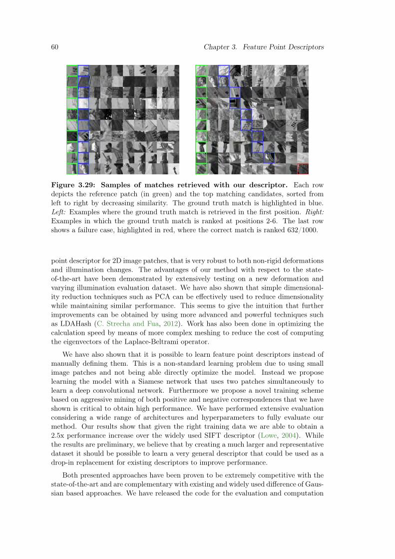
60 Chapter 3. Feature Point Descriptors
Figure 3.29: Samples of matches retrieved with our descriptor. Each rowdepicts the reference patch (in green) and the top matching candidates, sorted fromleft to right by decreasing similarity. The ground truth match is highlighted in blue.Left: Examples where the ground truth match is retrieved in the first position. Right:Examples in which the ground truth match is ranked at positions 2-6. The last rowshows a failure case, highlighted in red, where the correct match is ranked 632/1000.
point descriptor for 2D image patches, that is very robust to both non-rigid deformationsand illumination changes. The advantages of our method with respect to the state-of-the-art have been demonstrated by extensively testing on a new deformation andvarying illumination evaluation dataset. We have also shown that simple dimensional-ity reduction techniques such as PCA can be effectively used to reduce dimensionalitywhile maintaining similar performance. This seems to give the intuition that furtherimprovements can be obtained by using more advanced and powerful techniques suchas LDAHash (C. Strecha and Fua, 2012). Work has also been done in optimizing thecalculation speed by means of more complex meshing to reduce the cost of computingthe eigenvectors of the Laplace-Beltrami operator.
We have also shown that it is possible to learn feature point descriptors instead ofmanually defining them. This is a non-standard learning problem due to using smallimage patches and not being able directly optimize the model. Instead we proposelearning the model with a Siamese network that uses two patches simultaneously tolearn a deep convolutional network. Furthermore we propose a novel training schemebased on aggressive mining of both positive and negative correspondences that we haveshown is critical to obtain high performance. We have performed extensive evaluationconsidering a wide range of architectures and hyperparameters to fully evaluate ourmethod. Our results show that given the right training data we are able to obtain a2.5x performance increase over the widely used SIFT descriptor (Lowe, 2004). Whilethe results are preliminary, we believe that by creating a much larger and representativedataset it should be possible to learn a very general descriptor that could be used as adrop-in replacement for existing descriptors to improve performance.
Both presented approaches have been proven to be extremely competitive with thestate-of-the-art and are complementary with existing and widely used difference of Gaus-sian based approaches. We have released the code for the evaluation and computation

3.4. Summary 61
of the DaLI descriptor3 to encourage other researchers to compare against and use ourdescriptor in other applications. While we have not at the time of this writing releasedthe code for our deep descriptor framework, we intend to release it for the same reasons.
3http://www.iri.upc.edu/people/esimo/research/dali/


Chapter 4
Generative 3D Human Pose Models
In this chapter we give an overview of different models for 3D Human Pose estimation inorder of increasing complexity and expressiveness. This is not meant to be a completelist and only mentions models used throughout the course of this thesis. In particularwe shall discuss linear latent models, Directed Acyclic Graph (DAG) models, and wewill give a slightly longer description of the Geodesic Finite Mixture Model (GFMM).
4.1 Introduction
There has been a long tradition of generative models in the task of 3D human poseestimation. This is due to the space of possible 3D poses being extremely large. Addi-tionally, for 3D pose estimation there is no natural grid such as pixels used in 2D poseestimation. This makes it unnatural to define discriminative models such as the picto-rial structures model (Felzenszwalb and Huttenlocher, 2005) widely used in the 2D forthe 3D case. Furthermore, when tracking 3D poses, there is a strong spatial pose priorwhich encourages searching the solution space near the solution of the previous frame,which can be incorporated elegantly into generative models.
In this chapter we shall focus on three different approaches used in this thesis: linearlatent models, Directed Acyclic Graph (DAG) models, and Geodesic Finite MixtureModels (GFMM) We will give a special focus to the latter model which is a novel modelproposed in this thesis. For all these poses we consider the static scenario, i.e., we donot consider motion nor any other temporal information. Additionally all models makeuse of latent variables to model the pose.
Each model has a different set of strengths and weaknesses. We focus on four differ-ent model attributes: complexity, scalability, consistency, and whether it is modellingthe Probability Density Function (PDF) of the data. Complexity roughly correspondsto the level of technical and algorithmic complexity of the model. As to be expected,linear models have very low complexity in both formulation and speed, however, theytend to be much weaker representations. As dataset sizes are getting larger and larger,scalability or the ability of the model to benefit from large amounts of data is becom-ing more and more important. Additionally for 3D human pose estimation, we know
63

64 Chapter 4. Generative 3D Human Pose Models
(a) Probability Density Function (b) Trajectory reconstruction
(c) Random trajectories drawn from the model
Figure 4.1: Example of a GPDM with a 3-dimensional latent space. Modelare learnt from a walking sequence of 2.5 gaits on the CMU mocap dataset (mo-cap.cs.cmu.edu). Figures reproduced from (Wang et al., 2005).
the data lies on a manifold for a given individual. Consistency refers to whether or notan algorithm is able to generate poses only on this manifold, or if it can erroneouslyalso generate outside the manifold and thus generate non-anthropomorphic poses. Fi-nally, not all models attempt to represent the PDF of the data. In particular linearmodels are unable to, while more expressive models are able to. Although there aremore model attributes that can be taken into account, we find that these four are themost representative of 3D pose models.
For the entire chapter we shall write a 3D pose as the vector x = [pT1 , · · · ,p
Tnv],
where pi are the 3D positions of the skeleton joints. In general the objective is to modelthe distribution of these poses, that is p(x).

4.2. Related Work 65
4.2 Related Work
One of the more successful families of models for 3D human pose estimation have beenthe Gaussian Process family of models. Of which the most important is the GaussianProcess Latent Variable Model (GPLVM) (Lawrence, 2005), in which a continuouslow-dimensional latent space is learnt for a single cycle of a motion. This has beenextended to dynamics with the Gaussian Process Dynamic Model (GPDM) proposedby Wang et al. (Wang et al., 2005; Urtasun et al., 2006; Wang et al., 2008; A. Yao andUrtasun, 2011), which was also extended to include topological constraints (Urtasunet al., 2007). A visualization of a 3-dimensional GPDM is shown in Fig. 4.1. Hierarchicalvariants (hGPLVM) have also been used in a tracking by detection approach (Andrilukaet al., 2010). However, Gaussian Processes do not scale well to large datasets due to theirO(n3) complexity for prediction. Sparse approximations do exist (Quiñonero-candelaet al., 2005), but in general do not perform as well.
There have been other approaches such as learning Conditional Restricted Boltz-mann Machines (CRBM) (Taylor et al., 2010). However, these methods have a verycomplex learning procedure that makes use of several approximations and thus it is noteasy to train good models. Li et al. (Li et al., 2010) proposed the Globally CoordinatedMixture of Factor Analyzers (GCMFA) model which is similar to the GPLVM in thesense it is performing a strong non-linear dimensionality reduction. Yet, as in GPLVMmodels it does not scale well to large datasets. A more simple approach would be theGaussian Mixture Model (GMM) that have been used extensively to encode the rela-tionship between joints (Sigal et al., 2004; Daubney and Xie, 2011; Sigal et al., 2012).This is usually done in the angular space. However, as this space is not a vector spacedue to an inherent periodicity, they introduce heuristics to mitigate the effect it hason the GMM. On the other hand our proposed GFMM does not have this issue andadditionally provides a much better approximation of the underlying manifold, withoutany notable computational slowdown.
Additionally recently there have been many development on statistics on Rieman-nian manifolds (Pennec, 2006) that have made their way into computer vision (Fletcheret al., 2004; Pennec et al., 2006; Davis et al., 2007), and in particular human mo-tion (Sommer et al., 2010; Brubaker et al., 2012). The most popular model is thePrincipal Geodesic Analysis (PGA) model (Fletcher et al., 2004), in which the data isprojected onto a linear space which is an approximation of the manifold. As this spaceis linear, another linear model, in particular a linear latent model, can be constructedin this approximated space. While this is a simple scalable and consistent approach, itis not modelling a probability density function.
Not all work has been done on joint-based models. As it is quite common to usesilhouettes for 3D human pose tracking, shape-based models have been also proposed.Some of the more simple ones model the body with a set of cylinders which are fitted toa joint model (Sigal et al., 2004, 2012). However, there do exist approaches that directlywork with 3D meshes obtained from laser scans. One of the more well-known approachesapplies a Principal Component Analysis (PCA) to the 3D meshes (Anguelov et al., 2005;Hasler et al., 2009). An example of 3D scans is shown in Fig. 4.2. The downside of usingsilhouettes to match 3D mesh models is that it is usually dependent on backgroundsubtraction in order to get reliable silhouette estimates. On the other hand the jointbased models we consider can be used with other types of image evidence as we willshow in the next chapter.

66 Chapter 4. Generative 3D Human Pose Models
Figure 4.2: Examples of 3D body shape scans. These scans are used to obtaina set of deformation basis to represent body shape and 3D pose independently. Figurereproduced from (Hasler et al., 2009).
Model Complexity Scales? Consistent? PDF?
GMM (Sigal et al., 2004) Low Yes No Yes
PGA (Fletcher et al., 2004) Low Yes Yes No
GPLVM (Lawrence, 2005) Low No No Yes
GPDM (Wang et al., 2005) Medium No No Yes
hGPLVM (Andriluka et al., 2010) Medium No No Yes
CRBM (Taylor et al., 2010) High Yes No Yes
GCMFA (Li et al., 2010) High No No Yes
PCA Low Yes No No
DAG Medium Yes No Yes
GFMM Low Yes Yes Yes
Table 4.1: Comparison of different generative pose models. We analyze severalcommonly used human pose models. We consider the complexity of the models whichwe classify as low, medium or high. Models are considered to scale if they can handlewell large amounts of data (∼100k samples) and to be consistent if they use geodesicdistances instead of other metrics. Additionally we show whether or not a model isactually modelling the Probability Density Function (PDF) of the data. The bottomthree correspond to the models used in this thesis.
We show an overview of the aforementioned models in Table 4.1. We focus on fourmodel attributes: complexity, scalability, consistency, and whether or not the modelrepresents the Probability Density Function (PDF) of the data. We also include thethree models used in this thesis: latent linear model (PCA), Directed Acyclic Graph(DAG) and Geodesic Finite Mixture Model (GFMM). We can see that our models canall scale well to large data while having a medium to low complexity. Additionally theGFMM is consistent with the 3D human pose manifold.

4.3. Linear Latent Model 67
4.3 Linear Latent Model
Latent linear models are well known in the field of 3D pose estimation and shape recov-ery (Moreno-Noguer et al., 2009, 2010; Moreno-Noguer and Porta, 2011; Moreno-Noguerand Fua, 2013). Their extremely low complexity makes them very attractive for manydifferent applications. They consist in finding a linear transformation that projects datapoints to a, generally smaller, latent space. This is very useful as the true degrees offreedom of high dimensional data is usually much smaller than the dimensionality ofthe data. In general, there is no linear mapping between the pose manifold and the 3Dpose, however, the coarse approximation can be considered sufficient when combinedwith additional constraints such as illumination (Moreno-Noguer and Fua, 2013).
One of the more simple yet widely used approaches consists in finding a linear latentspace using Principal Component Analysis (Tenenbaum et al., 2000). This consists infinding a new linear basis for the data where the vectors are sorted by covariance. Bythen discarding the vectors with lower covariance it is possible to find a lower dimensionlinear subspace that conserves most of the data variability. In the context of deformableobject, the vectors of the new basis can be interpreted as different deformation modesof the object. This approach is unsupervised, i.e., no labels are needed for the data.An alternative is Linear Discriminant Analysis, in which a projection that attempts tomaximize the difference between the class of each sample is found. This is a supervisedapproach, that is, each sample has a label that we wish to predict.
Deformation Modes
We first assume that the 3D pose can be represented as a linear combination of a mean3D pose x0 and nm deformation models Q = [q1, · · · ,qnm ]
x = x0 +
nm∑
i=1
αiqi = x0 +Qα , (4.1)
where α = [α1, . . . , αnm ]T are the unknown weights that define the current 3D pose and
can be interpreted as parameters of the learnt latent space corresponding tho the pose x.The matrix Q can be found by simply calculating the eigenvalues of the covariance
of the training data. Assuming we have N poses xi we can rewrite them in matrix formas
X =
(x1 − x0)T
(x2 − x0)T
...
(xN − x0)T
, (4.2)
where x0 =1N
∑
i xi.The covariance C of the training data can then be calculated by
C =1
N − 1XTX . (4.3)
The eigenvectors V and eigenvalues λ can then be computed by
V−1CV = diag(λ) . (4.4)

68 Chapter 4. Generative 3D Human Pose Models
5 10 15 20 25 30 35 400.99
0.991
0.992
0.993
0.994
0.995
0.996
0.997
0.998
0.999
1
nm
Re
lative
Co
va
ria
nce
Figure 4.3: Effect of σthreshold in linear latent models. We plot how the parame-ter σthreshold affects the amount of covariance retained or relative covariance of the datafor the HumanEva walking action. In particular with nm = 21 we are able to retain99.99% of the covariance.
Without loss of generality we can assume the eigenvectors V are sorted in descendingorder by their eigenvalues λ.
Finally the matrix Q is just the first nm vectors of the eigenvectors V. As a criteriafor selecting the value of nm, the percent of the total variance explained by those vectorscan be used. Thus nm can be chosen by
argminnm
nm subject to σthreshold <
∑nm
i=1 di∑N
i=1 di. (4.5)
Thus instead of choosing the value of nm directly, it is chosen based on a more inter-pretable threshold σthreshold, which is the only hyperparameter of the model. Typicalvalues for σthreshold are around 0.99.
Results
We plot the effect of σthreshold in Fig. 4.3. This is the only hyperparameter of themodel and is critical for good performance as it serves as a lower-bound for 3D poseestimation error. From our experiments we found that setting nm = 21, correspondingto σthreshold = 0.9999, offers a good balance between dimensionality and low error. Wealso show a qualitative example of how the dimensionality affects the reconstructionquality in Fig. 4.4.
The main advantage of these linear models is they are very fast to compute and veryeasy to use. They are completely unsupervised and depend on a single hyperparameter.The main disadvantage is they only allow for linear relationships and are not trulymodelling p(x), i.e., they only model a mapping, not an actually Probability DensityFunction (PDF). Additionally were we to sample from the latent space α there is noguarantee that the poses will be anthropomorphic or human-like. Thus if samplingadditional criteria will have to be used to select only the anthropomorphic poses.
In Section 5.3 we shall show an application in which we benefit from the linearformulation. In particular we are able to combine the linear pose model with a linear

4.4. Directed Acyclic Graphs 69
Dimension of the Latent Space nm
1 2 3 4 5
−1200−1000
−800−600
−200 0 200
0
200
400
600
800
1000
1200
1400
1600
−1200−1000
−800−600
−200 0 200
0
200
400
600
800
1000
1200
1400
1600
−1200−1000
−800−600
−200 0 200
0
200
400
600
800
1000
1200
1400
1600
−1200−1000
−800−600
−200 0 200
0
200
400
600
800
1000
1200
1400
1600
−1200−1000
−800−600
−200 0 200
0
200
400
600
800
1000
1200
1400
1600
6 7 8 9 10
−1200−1000
−800−600
−200 0 200
0
200
400
600
800
1000
1200
1400
1600
−1200−1000
−800−600
−200 0 200
0
200
400
600
800
1000
1200
1400
1600
−1200−1000
−800−600
−200 0 200
0
200
400
600
800
1000
1200
1400
1600
−1200−1000
−800−600
−200 0 200
0
200
400
600
800
1000
1200
1400
1600
−1200−1000
−800−600
−200 0 200
0
200
400
600
800
1000
1200
1400
1600
Figure 4.4: Dimensionality of the Linear Latent Space. We show the effects ofthe dimensionality of the linear latent space for reconstructing. We show the groundtruth in black and the reconstructed pose for nm = {1, . . . , 10}. The first three dimen-sions serve to appropriately position the joints. Additional dimensions improve smallerdetails such as matching the hands and the feet.
camera projection model in order to project noisy 2D joint observations into the latentspace. As the formulation is linear, there is an exact solution, which generates a set of3D hypothesis that can be used to perform 3D pose estimation.
4.4 Directed Acyclic Graphs
Using probabilistic graphical models is very common in computer vision. In particularstar-shaped models (Felzenszwalb et al., 2008, 2010) and tree-shaped models (Yang andRamanan, 2011) have been widely used as exact inference can be performed. In the caseof general graphical models, inference is no longer exact due to the presence of loopsand must be performed by message passing algorithms (Sigal et al., 2012; Andrilukaet al., 2012). We instead opt to use Directed Acyclic Graphs (DAG), that can capturemore complicated relationships in comparison to tree models while still having exactinference, as there no loops in the graphical model.
This model attempts to characterize p(x) through a latent space. That is p(x) is notmodelled directly, instead it is modelled as p(x) = p(x|h)p(h) where h is a latent space.In order to be tractable the poses are discretized using a clustering algorithm such ask-means into a set of base poses XL. Additionally we define the lower dimensional

70 Chapter 4. Generative 3D Human Pose Models
latent space as another discrete set H. The problem can then be seen as learning acompression function φ(XL) : XL → H that maps points in the high dimensional local3D pose space to a lower dimensional space.
Discrete Joint Model
In order to obtain the discrete pose set XL the x poses in 3D are first transformed to alocal reference such that they only represent local deformations. Then they are mappedfrom the R
N×3 continuous pose space x to a discrete domain by doing vector quantiza-tion of groups of 3D joint positions. More specifically, the joints are grouped into fivecoarse parts: right arm (ra), left arm (la), right leg (rl), left leg (ll) and torso+head(th). Thus, every pose can be mapped to a discrete vector T = [ra, la, rl, ll, th] ∈ K5
where ra, la, rl, ll, th are cluster indexes belonging to K = {1, 2, .., k} of the correspond-ing 3D joint positions.
We will now define a joint distribution over latent variables H ∈ H = {1, .., n}(where n is the number of latent states), and observed variables T . The model is givenby the following generative process:
- Sample a latent state i according to p (h0)
- For all the parts associated with arm and leg positions, sample discrete locations:< ra, la, rl, ll > and states < j, l,m, n > according to the conditional distribu-tions: p (hra = j, ra | i), p (hla = l, la | i), p (hrl = m, rl | i) and p (hll = n, ll | i)
- Sample a pair of latent states: < q,w > (associated with the positions of theupper body and lower body joints) according to p (hu = q | hra = j, hla = l) andp (hl = w | hrl = m,hll = n)
- Sample a discrete location th and a state r from p(h(th) = r, th | hu = q, hl = w
)
Given this generative model we define the probability of a discrete 3D positionT = [ra, la, rl, ll, th] as:
p (T ) =∑
H
p (T,H)
=∑
H
p (h0) p (hra, ra | h0) p (hla, la | h0)
p (hrl, rl | h0) p (hll, ll | h0) p (hu | hra, hla)
p (hll, ll | h0) p (hu | hra, hla)
p (hl | hrl, hll) p (hth, th | hu, hl) .
The graphical model corresponding to this joint distribution is illustrated in Fig. 4.5a,where the graph G specifies the dependencies between the latent states. Since H isunobserved, Expectation Maximization can be used to estimate the model parametersfrom a set of training poses. Given that G is a Directed Acyclic Graph we can computeall required expectations efficiently with dynamic programming (Huang, 2008). Oncewe have learned the parameters of the model we define our compression function to be:
φ(XL) = argmaxH
p(XL, H
),
and our decompression function to be:
φ−1(H) = argmaxXL
p(XL, H
).

4.4. Directed Acyclic Graphs 71
hth
hu hl
hra hla hrl hll
h0
T th
ra la
llrl
G
(a) UL grouping
hth
hr hl
hra hrl hla hll
h0
T th
ra la
llrl
G
(b) RL grouping
Figure 4.5: Directed Acyclic Graph models for 3D human pose. We usea probabilistic graphical model with latent variables G to represent the possible 3Dhuman pose T from a large set of discrete poses. Latent variables can either be mappedto the conjoint motion of various parts or be used as internal states containing internalstructure of the pose. We show two different type of body part groupings: (a) Upperand Lower body grouping, and (b) Right and Left side grouping.
States 1 2 3 4 5 6 7
UL 123 108 87 64 61 51 46
RL 123 107 84 68 77 49 49
Table 4.2: Influence of the number of latent states. We evaluate them using theaverage reconstruction error (in mm). We compare the upper-lower grouping (UL) toa right-left grouping (RL), which can be seen to perform roughly the same. The valuesused are highlighted in bold.
Note that the decompression function is not technically speaking the true inverse ofφ(XL), clearly no such inverse exists since φ(XL) is many to one. However, we canregard φ−1(H) as a “probabilistic inverse” that returns the most probable pre-image ofH. Our compression function maps points in K5 to points in H8. For example, whenk=300 and n=9 we reduce the search space size from 1011 to 106.
Results
One of the major concerns when building the DAG is what structure the graph shouldhave. This is an open problem and in general is left as a design decision. We experimentwith using two different groupings: grouping right and left sides of the body (RL), andgrouping upper and lower body (UL). An overview of both groupings can be seen inFig. 4.5. Another hyperparameter is the number of latent states for each node. In orderto minimize the number of hyperparameters we use the same number of states for allnodes. We experiment on the HumanEVA dataset (Sigal et al., 2010b). We evaluate

72 Chapter 4. Generative 3D Human Pose Models
0 5 10 15 20 25 30 35 40 45 5018
20
22
24
26
28
30
32
34
36
38
Iteration
Lo
g−l
ike
liho
od
Val Error
Train Error
(a) Training of the model (b) Samples from the model
Figure 4.6: Directed Acylcic Graph (DAG) model training and sampling.We train the DAG model for the training action with 6 latent states and UL grouping.(a) Log-likelihood of the model for the training and validation splits. (b) Samples fromthe trained model. As we have trained with all three subjects simultaneously we seethree different body sizes among the samples.
using the method by compressing and decompressing the testing poses to obtain thereconstruction error ǫrec defined as
ǫrec(XL) = XL − φ−1(φ(XL)) . (4.6)
We show results for both groupings and number of latent states in Table 4.2. We can seethat in this case both groupings perform nearly the same. While it is likely the graphicalstructure chosen is not optimal, the architecture does not seem to influence to heavilyin the results. On the other hand the number of latent states is very important to beable to accurately model human pose. However, adding more latent states increases thesize of the model, causing it to overfit. For our experiments we chose 6 latent stateswith a Upper and Lower body grouping (UL) that seems to provide a reasonable mixof good performance without having too many degrees of freedom.
The results of training the model can be seen in Fig. 4.6. We can see with 6 latentstates per node the model overfits fairly quickly. We rely on a validation split in order toavoid the overfitting. Samples taken from the model can be seen in Fig. 4.6b. As we trainwith all 3 subjects simultaneously, three different body sizes can be identified. Most ofthe variability is, as expected of the walking action, located at the limb extremities.
The advantage of this model with respect to the linear latent model is clear: weare actually able to model and sample from p(x) through the latent space. Thereforewe do not need to perform any additional selection based on anthropomorphism norother criterion. However, the model still has several disadvantages. Namely we aremodelling the pose directly in 3D coordinates. This means that limb lengths may varyfor different individuals, i.e., it is not an individual agnostic representation. Additionallythe discretization is also not exempt of issues. It creates artefacts in the 3D pose whensampling in addition to increase the number of hyperparameters of the model. Despitethis, we believe it is a step forward with respect to using linear latent models for thetask of 3D pose generation.

4.5. Geodesic Finite Mixture Models 73
−3 −2 −1 0 1 2 3
−3
−2
−1
0
1
2
3
(a) SO(2) Geodesics (b) Geodesic Finite Mixture Model
Figure 4.7: Geodesics and Mixture Models. (a) Representation of geodesics onthe S2 manifold. The tangent space ensures that ‖ logo(x)‖ is the true geodesic distance
of −→ox. However, ‖ logo(a)− logo(b)‖ is not the geodesic distance of−→ab. (b) Illustration
of the proposed mixture model approach. Each mixture component has its own tangentspace, ensuring the consistency of the model while minimizing accuracy loss.
4.5 Geodesic Finite Mixture Models
In order to deal with problems that arose when using both the linear latent modeland the Directed Acyclic Graph (DAG) model, we investigated into using Riemannianmanifolds for representing the pose and modelling directly on the manifold. This allowsus to obtain a individual-agnostic model in the continuous domain that can scale wellto large datasets. More importantly, this model is consistent with the human posemanifold, i.e., it will only generate poses that have no limb deformation.
It is well known that human motion can be represented as points on a Riemannianmanifold (Brubaker et al., 2012; Sommer et al., 2010). We consider the task of obtaininga probabilistic generative model of the poses, that is, approximate the ProbabilityDensity Function (PDF) of points on this manifold for a potentially large dataset.As we consider the situation in which the data lies on a known Riemannian manifold.We are able to create an efficient completely data-driven algorithm consistent with themanifold, i.e., an algorithm that yields a PDF defined exclusively on the manifold.
A standard procedure to operate on a manifold is to use the logarithmic mapto project the data points onto the tangent space of the mean point on the mani-fold (Fletcher et al., 2004; Sommer et al., 2010; Huckemann et al., 2010). After thislinearization, Euclidean statistics are computed and projected back to the manifold us-ing the exponential map. This process is iteratively repeated until convergence of thecomputed statistics. Unfortunately, while this approximation is effective to model datawith a reduced extent, it is prone to fail when dealing with data that covers wide re-gions of the manifold.
In the proposed finite mixture model, we overcome this limitation by simultaneouslyconsidering multiple tangent spaces, distributed along the whole manifold as seen inFig. 4.7. We draw inspiration on the unsupervised algorithm from (Figueiredo andJain, 2002), which given data lying in an Euclidean space, automatically computes thenumber of model components that minimize a message length cost. By representingeach component as a distribution on the tangent space at its corresponding mean onthe manifold, we are able to generalize the algorithm to Riemannian manifolds and atthe same time mitigate the accuracy loss produced when using a single tangent space.

74 Chapter 4. Generative 3D Human Pose Models
Furthermore, since our model is semi-parametric, we can handle an arbitrarily largenumber of samples. This is in contrast to existing non-parametric approaches (Pelletier,2005) whose complexity grows with the training set size.
In this section we will show that our manifold-based finite mixture model can beeffectively used both for non-linear data modeling and regression. In addition, we willshow that the modeling of articulated structures can greatly benefit from our approach,allowing for instance, hallucinating subsets of missing joints of the human body withoutany specific training.
Method
We next describe our approach, starting with some basic notions on Riemannian geom-etry and statistics on manifolds. We then integrate these tools in a mixture modelingalgorithm to build consistent generative models.
Manifolds, Geodesics and Tangent Spaces
Manifolds arise naturally in many real-world problems. One of the more well-known isthe manifold representing spatial rotations. For example, when studying human motion,it is a common practice to use the spatial rotations of the different body parts to obtain asubject-agnostic representation of the whole body pose. This is usually done with anglerepresentations that have an inherent periodicity and thus are not a vector space. Byconsidering the Riemannian manifold of spatial rotations it is possible to use tangentspaces as a local vector space representation, and use powerful statistical tools basedon Euclidean metrics. For an in depth description of Riemannian manifolds we referthe reader to (Boothby, 2003).
Geodesic distances, which we shall denote as d(·, ·), are the shortest distance alongthe manifold between two arbitrary points. This distance is generally not equivalent toan Euclidean one. The tangent space is a local vector space representation where theEuclidean distances between the origin and arbitrary points correspond to the geodesicdistances on the manifold. Yet, as seen in Fig. 4.7a, this correspondence does not holdfor two arbitrary points. A point v ∈ M on the tangent space TcM at c ∈ M canbe mapped to the manifold M and back to the TcM by using the exponential andlogarithmic maps respectively:
expp :TcM −→ M
v 7−→ expc (v) = x(4.7)
logp :M −→ TcM
x 7−→ logc (x) = v(4.8)
In general there is no closed-form of the expc and logc maps for an arbitrary man-ifold. There are, though, approximations for computing them in Riemannian mani-folds (Dedieu and Nowicki, 2005; Sommer et al., 2009). Additionally, efficient closed-form solutions exist for certain manifolds (Said et al., 2007). An interesting mappingfor us will be the one between the unit sphere S2 and its tangent space TcS
2. Letx = (x1, x2, x3)
⊤, y = (y1, y2, y3)⊤ be two unit spoke directions in S2 and v = (v1, v2)
⊤

4.5. Geodesic Finite Mixture Models 75
a point in TcS2. The expc and logc maps are in this case:
expc(v) = R−1c
(
v1sin ‖v‖
‖v‖, v2
sin ‖v‖
‖v‖, cos ‖v‖
)
(4.9)
logp(x) =
(
y1θ
sinθ, y2
θ
sinθ
)
(4.10)
where Rc is the rotation of c to the north pole, ‖v‖= (v21 + v22)1
2 , y = Rcx andθ = arccos(y3).
Statistics on Tangent Spaces
While it is possible to define distributions on manifolds (Pennec, 2006), we shall focuson approximating Gaussian PDFs using the tangent space. Since it is a vector space,we can compute statistics that, by definition of the tangent space, are consistent withthe manifold. For instance, the mean of N points xi on a manifold can be calculatedas (Karcher, 1977)
µ = argminc
N∑
i=1
d (xi, c)2 . (4.11)
This is optimized iteratively using the expc and logc maps,
µ(t+ 1) = expµ(t)
(
δ
N
N∑
i=1
logµ(t) (xi)
)
, (4.12)
until ‖µ(t+ 1)− µ(t)‖ < ǫ for some threshold ǫ, with δ being the step size parameter.Given the mean, it is then possible to estimate the covariance on the tangent space:
Σ =1
N
N∑
i=1
logµ(xi) logµ(xi)⊤ . (4.13)
Knowing the mean value and the concentration matrix (Γ = Σ−1) we can write thedistribution that maximizes entropy on the tangent space as a normal distributioncentered on the point µ ∈ M, corresponding to the origin (ν = 0) in the tangent space:
Nµ(ν, Σ−1) = a exp
(
−logµ(x)
⊤Σ−1 logµ(x)
2
)
(4.14)
where a is normalization term that ensures the normal distribution over the tangentspace integrates to unity. If TµM ≡ R
D this term simplifies to
a−1 =√
(2π)D det(Σ) . (4.15)
As the normalization term is dependent on the tangent space, it is not always easyto obtain. However, it is possible to approximate this normalization factor based onmaximum entropy criterion computed directly on the manifold (Pennec, 2006). Sincethis situation is very unusual, it is not further explored in this thesis.

76 Chapter 4. Generative 3D Human Pose Models
Unsupervised Finite Mixture Modeling
Our approach for fitting the mixture model relies on (Figueiredo and Jain, 2002), avariant of the EM algorithm that uses the Minimum Message Length criterion (MML)to estimate the number of clusters and their parameters in an unsupervised manner.
Given an input dataset, this algorithm starts by randomly initializing a large numberof mixtures. During the Maximization (M) step, a MML criterion is used to annihilatecomponents that are not well supported by the data. In addition, upon EM convergence,the least probable mixture component is also forcibly annihilated and the algorithmcontinues until a minimum number of components is reached. (Figueiredo and Jain,2002) is designed to work with data in an Euclidean space. To use it in Riemannianmanifolds, we modify the M-step as follows.
Each mixture component is defined by its mean µk and concentration matrix Γk =Σ−1k as a normal distribution on its own tangent space Tµk
M:
p(x|θk) ≈ Nµk
(0, Σ−1
k
)(4.16)
with θk = (µk,Σk). Remember that the mean µk is defined on the manifold M, whilethe concentration matrix Γk is defined on the tangent space Tµk
M at the mean νk = 0.Also note that the dimensionality of the space embedding the manifold is larger than
the actual dimension of the manifold, which in its turn is equal to the dimension ofthe tangent space. That is, dim(Embedding(M)) > dim(TcM) = dim(M) = D.This dimensionality determines the total number of parameters Dθ specifying eachcomponent, and, as we will explain below, plays an important role during componentannihilation process. For full covariance matrices it can be easily found that Dθ =D +D(D + 1)/2.
We next describe how the EM algorithm is extended from Euclidean to Riemmanianmanifolds. Specifically, let us assume that K components survived after iteration t− 1.Then, in the E-step we compute the responsibility that each component k takes forevery sample xi:
w(i)k =
αk(t− 1)p(xi|θk(t− 1))∑K
k=1 αk(t− 1)p(xi|θk(t− 1)), (4.17)
for k = 1, . . . ,K and i = 1, . . . , N , and where αk(t− 1) are the relative weights of eachcomponent k.
In the M-step we update the weight αk, the mean µk and covariance Σk for each ofthe components as follows:
αk(t) =1
N
N∑
i
w(i)k =
wkN
(4.18)
µk(t) = argminc
N∑
i=1
d
(N
wkw
(i)k x(i), c
)2
(4.19)
Σk(t) =1
wk
N∑
i=1
(
logµk(t)(x(i))
)(
logµk(t)(x(i))
)⊤w
(i)k (4.20)
After each M-step, we follow the same annihilation criterion as in (Figueiredo and Jain,2002), and eliminate those components whose accumulated responsibility wk is below aDθ/2 threshold. A score for the remaining components based on the Minimum Message
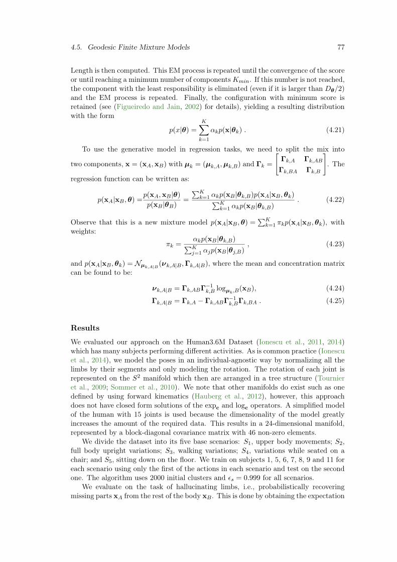
4.5. Geodesic Finite Mixture Models 77
Length is then computed. This EM process is repeated until the convergence of the scoreor until reaching a minimum number of componentsKmin. If this number is not reached,the component with the least responsibility is eliminated (even if it is larger than Dθ/2)and the EM process is repeated. Finally, the configuration with minimum score isretained (see (Figueiredo and Jain, 2002) for details), yielding a resulting distributionwith the form
p(x|θ) =K∑
k=1
αkp(x|θk) . (4.21)
To use the generative model in regression tasks, we need to split the mix into
two components, x = (xA,xB) with µk = (µk,A,µk,B) and Γk =
[
Γk,A Γk,AB
Γk,BA Γk,B
]
. The
regression function can be written as:
p(xA|xB,θ) =p(xA,xB|θ)
p(xB|θB)=
∑Kk=1 αkp(xB|θk,B)p(xA|xB,θk)
∑Kk=1 αkp(xB|θk,B)
. (4.22)
Observe that this is a new mixture model p(xA|xB,θ) =∑K
k=1 πkp(xA|xB,θk), withweights:
πk =αkp(xB|θk,B)
∑Kj=1 αjp(xB|θj,B)
, (4.23)
and p(xA|xB,θk) = Nµk,A|B(νk,A|B,Γk,A|B), where the mean and concentration matrix
can be found to be:
νk,A|B = Γk,ABΓ−1k,B logµk,B
(xB), (4.24)
Γk,A|B = Γk,A − Γk,ABΓ−1k,BΓk,BA . (4.25)
Results
We evaluated our approach on the Human3.6M Dataset (Ionescu et al., 2011, 2014)which has many subjects performing different activities. As is common practice (Ionescuet al., 2014), we model the poses in an individual-agnostic way by normalizing all thelimbs by their segments and only modeling the rotation. The rotation of each joint isrepresented on the S2 manifold which then are arranged in a tree structure (Tournieret al., 2009; Sommer et al., 2010). We note that other manifolds do exist such as onedefined by using forward kinematics (Hauberg et al., 2012), however, this approachdoes not have closed form solutions of the expc and logc operators. A simplified modelof the human with 15 joints is used because the dimensionality of the model greatlyincreases the amount of the required data. This results in a 24-dimensional manifold,represented by a block-diagonal covariance matrix with 46 non-zero elements.
We divide the dataset into its five base scenarios: S1, upper body movements; S2,full body upright variations; S3, walking variations; S4, variations while seated on achair; and S5, sitting down on the floor. We train on subjects 1, 5, 6, 7, 8, 9 and 11 foreach scenario using only the first of the actions in each scenario and test on the secondone. The algorithm uses 2000 initial clusters and ǫs = 0.999 for all scenarios.
We evaluate on the task of hallucinating limbs, i.e., probabilistically recoveringmissing parts xA from the rest of the body xB. This is done by obtaining the expectation

78 Chapter 4. Generative 3D Human Pose Models
(a) Scenario 1 (b) Scenario 2 (c) Scenario 3
(d) Scenario 4 (e) Scenario 5
Figure 4.8: Sampling from the Geodesic Finite Mixture Model. We samplefrom the different mixtures trained on each of the scenarios. For visualization pur-poses, we perform 3D reconstruction using the limb lengths of subject 1. Note thatthe mixtures themselves represent poses and are independent of limb lengths. For eachscenario, in the top left 30 samples are presented along with 5 particular examples. Wecan see there is a lot of diversity that our model is able to capture.

4.5. Geodesic Finite Mixture Models 79
Scenario 1 Scenario 2 Scenario 3
MGJE MJE MLLE MGJE MJE MLLE MGJE MJE MLLE
GFMM 0.446 105.8 0.0 0.468 110.1 0.0 0.349 81.7 0.0
vMF 0.481 114.5 0.0 0.568 134.8 0.0 0.470 110.2 0.0
1-TM 0.522 123.0 0.0 0.640 148.7 0.0 0.535 124.9 0.0
GMM 1.111 103.1 19.0 1.167 106.6 27.5 1.152 77.6 11.3
Scenario 4 Scenario 5
MGJE MJE MLLE MGJE MJE MLLE
GFMM 0.458 108.2 0.0 0.597 135.7 0.0
vMF 0.496 118.0 0.0 0.698 162.3 0.0
1-TM 0.548 130.2 0.0 0.765 175.1 0.0
GMM 1.272 101.0 14.2 1.401 127.3 24.8
Table 4.3: Comparing the Geodesic Finite Mixture Model (GFMM) withother approaches. We compare against von Mises Fisher distributions (vMF), asingle tangent space (1-TM) and an Euclidean Gaussian Mixture Model (GMM) in thelimb reconstruction task. We show results using three different metrics: Mean GeodesicJoint Error (MGJE), Mean Joint Error (MJE), and Mean Limb Length Error (MLLE).
of the posterior p(xA|xB,θ) using a combination of the conditional means (Eq. (4.24))at each tangent space with
xA = argminc
K∑
k=1
d(πkνk,A|B, c
)2(4.26)
We compare our method with von Mises Fisher distributions (vMF), a single tangentspace (1-TM) and a Gaussian Mixture Model in Euclidean space (GMM). To compen-sate the fact that our approach is individual-agnostic, was trained with the GMM withsame individual that was being tested. We define three metrics: Mean Geodesic JointError (MGJE), that accounts for the rotation error; Mean Joint Error (MJE), repre-senting the Euclidean distance with the ground truth in mm; and Mean Limb LengthError (MLLE), which is the amount of limb length deformation in mm. All four modelsare trained using exactly the same parameters for all scenarios. The results are sum-marized in Table 4.3. Observe that while the MJE is similar for both our method andGMM, our approach has roughly one third of the MGJE error. Additionally, as ourmodel is coherent with the manifold, there is no limb deformation (MLLE). Our modelalso consistently outperforms the vMF and 1-TM approaches, which once again showsthat multiple tangent spaces with Gaussians can better capture the underlying distri-bution. The 1-TM approach has the worst MJE error but we can see it has a MGJEmuch closer to our model than the GMM. We also outperform the vMF model. Weshow four specific examples of the estimated distributions for our model in Fig. 4.9.
In summary we have proposed a novel data-driven approach for modeling the prob-ability density function of data located on a Riemannian manifold. By using a mixture

80 Chapter 4. Generative 3D Human Pose Models
(a) Scenario 1 (b) Scenario 2 (c) Scenario 3
(d) Scenario 4 (e) Scenario 5
Figure 4.9: Human pose regression with the GFMM. We use the trained mix-tures to perform regression on the left arm (3 limbs) of subjects on the Human3.6Mdataset. On the left we plot 30 random samples from the full mixture. On the top-rightwe plot 30 random samples from the mixture of the conditional distribution correspond-ing to a particular frames. On the bottom-right the mean of the mixture is shown in red.The black lines indicate the input sample. As shown in Scenario 4, the distribution canbe multimodal, however, one of the modes is very close to the true limb position.
of distributions, each with its own tangent space, we are able to ensure the consistencyof the model while avoiding most of the linearization error caused by using one singletangent space. The approach has been experimentally validated on various syntheticexamples that highlight their ability to both correctly approximate manifold distribu-tions and discover the underlying data structure. Furthermore, the approach has beentested on a large and complex dataset, where it is shown to outperform the traditionallyused Euclidean Gaussian Mixture Model, von Mises distributions and using a singletangent space in a regression task.
4.6 Summary
In this chapter we have presented three generative models of varying complexity andexpressiveness that are suitable for 3D human pose. The linear latent model finds alinear transformation of the data that maximizes the covariance of the training data.

4.6. Summary 81
The Directed Acyclic Graph (DAG) model on the other hand defines a joint distributionover pose and a set of latent variables p(XL, H), and calculates expectations withdynamic programming. Finally the Geodesic Finite Mixture Model (GFMM) directlyrepresents the data p(x) with a Gaussian Mixture Model in which each mixture isdefined on a separate local linear representation of the pose manifold.
Each have different strengths and weaknesses making them adequate for differenttasks. The linear latent model is very simple and fast to calculate, however, it doesnot necessarily produce realistic poses. The DAG model is able to model the posesefficiently, but it relies on using discrete states for the poses. The GFMM on the otherhand is a fully continuous generative model that is very efficient to sample on, but itrelies on having a large amount of data to be able to train good models. In general,the optimal model for a particular framework or problem will depend heavily on manydifferent constraints such as time complexity, or required accuracy. The approaches wehave discussed in this chapter have very different properties that allow them to covermost if not all usage cases.
In the next chapter we will show full end-to-end systems that are able to exploitthese different generative models to predict 3D human poses from single images.


Chapter 5
3D Human Pose Estimation
Estimating the 3D human pose using a single image is a severely under-constrainedproblem, as many different body poses may have very similar image projections. In thischapter we shall explain two different methods for approaching this problem. The firstone consists of estimating the 2D human pose, and then propagating the uncertaintyof the 2D estimation to 3D, where the hypothesis can be disambiguated based onanthropomorphism to obtain a single solution. The second approach is based on jointlyestimating the 2D and 3D pose using a combination of 2D discriminative body partdetectors with a strong 3D generative model. By iteratively generating hypothesis andthen ranking them based on how well they match the detector responses, we are ableto find a single 2D and 3D human pose estimation.
5.1 Introduction
Computer vision has always had a focus on problems centered around humans and theirenvironment. One of the more traditional computer vision problems has been thatof detecting humans in static images (Dalal and Triggs, 2005). This problem was thenextended to also estimating the 2D human pose from these images in which the PictorialStructures (Felzenszwalb and Huttenlocher, 2005) and its variations (Ramanan, 2006;Andriluka et al., 2009; Yang and Ramanan, 2011; Andriluka et al., 2012) played afundamental role. However, as humans are not 2D structures, many ambiguities cannot be resolved with pure 2D models, leading to the advent of the 3D human poseestimation problem. In order to simplify the problem, most approaches either tacklethe 3D human pose tracking problem (Lawrence and Moore, 2007; Urtasun et al., 2006;Zhao et al., 2011; Andriluka et al., 2010), the multiview 3D pose estimation problem (Boand Sminchisescu, 2010; Burenius et al., 2013; Kazemi et al., 2013) (shown in Fig. 5.1)or a combination of both (Daubney and Xie, 2011; Yao et al., 2012a). On the otherhand the single image monocular problem has only recently gained popularity.
In order to disambiguate the problem, one common approach is to assume that an
83

84 Chapter 5. 3D Human Pose Estimation
Figure 5.1: Example of a multiview 3D pose estimation approach. In this ap-proach a random forest is first used to classify each pixel in each image as belongingto a part or the background. The results are then back-projected to a 3D volume.Corresponding mirror symmetric parts are found across views by using latent vari-ables. Finally, a part-based model is used to estimate the 3D pose Figure reproducedfrom (Kazemi et al., 2013).
underlying deformation model is available. Linear models (Balan et al., 2007) or sophis-ticated dimensionality reduction methods have been used for this purpose (Lawrenceand Moore, 2007; Sminchisescu and Jepson, 2004; Urtasun et al., 2006). Alternatively,other techniques have focused on learning the mapping from 2D image observations to3D poses (Okada and Soatto, 2008; Rogez et al., 2008; Sigal et al., 2009). In any event,most of these generative and discriminative approaches rely on the fact that 2D fea-tures, such as edges, silhouettes or joints may be easily obtained from the image.
In this thesis, we get rid of the strong assumption that data association may be easilyachieved, and propose two novel approaches for estimating the 3D pose of a personfrom a single image acquired with a calibrated but potentially moving camera. For thispurpose we use a HOG-based discriminative appearance model trained independentlyon the PARSE dataset for 2D human pose estimation (Yang and Ramanan, 2011).By training the 2D appearance model independently, we are able to avoid overfittingthe model to the 3D human pose estimation datasets that have very low appearancevariability. Poor generalization is a general trait of models with appearance trainedexclusively on the 3D dataset (Sminchisescu and Jepson, 2004).
The first approach we present consists of initially using a 2D human pose estimationalgorithm (Yang and Ramanan, 2011) to obtain a noisy estimation of the 2D pose. Thenby combining a linear latent pose model with a linear camera projection model, we areable to project the noisy 2D pose estimation into the latent space with a closed-formformulation to obtain a large set of pose hypothesis. As the linear latent model is nota probabilistic model, we rely on an anthropomorphism classifier to disambiguate theresulting poses to obtain a final solution. By exploiting linear formulations and fastclassifiers, the algorithm is extremely efficient with the runtime dominated by the 2Dhuman pose estimation. The downside of this approach is the fact it is a pipelinedapproach, i.e., if the 2D pose estimation is incorrect, the 3D pose estimation will alsobe incorrect.
Our second approach relaxes the hypothesis that we have a 2D human pose esti-mation and instead relies directly on a bank of discriminative independent 2D bodypart detectors. We use a Bayesian formulation very similar to the pictorial structuresmodel which consists of the aforementioned 2D body part detectors in conjunction witha strong 3D pose generative model. In particular we use a Directed Acyclic Graph(DAG) to model the pose. By alternatively sampling from the generative model and

5.2. Related work 85
Figure 5.2: Convolutional Neural Network for 3D Pose Estimation. Thenetwork is initially pre-trained for the 2D human detection task using layers fcd1,fcd2, and fcd3. Afterwards training is continued for the 3D human pose estimationtask, which is treated as a regression problem and uses layers fcr1, fcr2, and fcr3.Figure reproduced from (Li and Chan, 2014).
then evaluating using the discriminative model we are able to jointly estimate the 2Dand 3D pose.
We evaluate both of our approaches numerically on the HumanEva dataset (Sigalet al., 2010b) and qualitatively on the TUD Stadtmitte sequence (Andriluka et al.,2010). Results for both approaches are competitive with the state-of-the-art despiteour relaxation of restrictions.
5.2 Related work
Without using prior information, monocular 3D human pose estimation is known to bean ill-posed problem. In order to be disambiguate between the possible solutions, manymethods to favor the most likely shapes have been proposed.
One of the most straightforward approaches consists of modeling the pose deforma-tions as linear combinations of modes learned from training data (Balan et al., 2007).Since linear models are prone to fail in the presence of non-linear deformations, more ac-curate dimensionality reduction approaches based on spectral embedding (Sminchisescuand Jepson, 2004), Gaussian Mixtures (Howe et al., 1999) or Gaussian Processes (Ur-tasun et al., 2006; Lawrence and Moore, 2007; Zhao et al., 2011) have been proposed.However, these approaches rely on good initializations, and therefore, they are typicallyused in a tracking context. Other approaches follow a discriminative strategy and uselearning algorithms such as support vector machines, mixtures of experts or randomforest to directly learn the mappings from image evidence to the 3D pose space (Agar-wal and Triggs, 2006; Okada and Soatto, 2008; Rogez et al., 2008; Sigal et al., 2009).
Most of the aforementioned solutions, though, oversimplify the 2D feature extractionproblem, and typically rely on background subtraction approaches or on the fact thatimage evidence, such as edges or silhouettes, may be easily obtained from an image, oreven assume known 2D (Salzmann and R.Urtasun, 2010; Ramakrishna et al., 2012).
With regard to the problem of directly predicting 2D poses on images, we find that

86 Chapter 5. 3D Human Pose Estimation
Uncertain 2D Detection Ambiguous 3D Poses Disambiguated Pose
−5000500100015002000−1000−5000
−500
0
500
1000
1500
500600700800900−600−400−200
0
200
400
600
800
1000
1200
1400
1600
Figure 5.3: 3D human pose estimation from noisy observations. The leftimage shows the bounding box results of a body part detector and green dots indicatethe true position of the joints. Note, in the middle, how the bounding box centers donot match the joint positions. Using the heat map scores of the classifier we representthe output of the 2D detector by Gaussian distributions, as shown on the right. Usingthe distribution of all the joints we sample the solution space and propose an initial setof ambiguous poses. By simultaneously imposing geometric and kinematic constraintsthat ensure the anthropomorphism, we are able to pick an accurate 3D pose (shown inmagenta on the right) very similar to the ground truth (black).
one of the most successful methods is the pictorial structure model (Felzenszwalb andHuttenlocher, 2005) (later extended to the deformable parts model (Felzenszwalb et al.,2008)), which represents objects as a collection of parts in a deformable configurationand allows for efficient inference. Modern approaches detect each individual part usingstrong detectors (Andriluka et al., 2009; Singh et al., 2010; Tian and Sclaroff, 2010; Yangand Ramanan, 2011) in order to obtain good 2D pose estimations. The deformableparts model has also been extended to use 3D models for 3D viewpoint estimation ofrigid objects (Pepik et al., 2012).
Recently there has been an explosion in deep network approaches in the computervision community that have made their way to 3D human pose estimation from singleimages (Li and Chan, 2014) using the architecture shown in Fig. 5.2. However, in generalmost works still focus on the 2D human pose estimation problem (Jain et al., 2014a;Toshev and Szegedy, 2014; Jain et al., 2014b). Currently 3D human pose estimationusing deep networks suffers from an overfitting to the unnatural images of the trainingdataset. That is, in order to obtain a 3D ground truth, the subjects wear specialclothing in conjunction with markers used in the 3D capture system. Appearancemodels learnt on these images do not generalize well to natural images. In contrast wepropose using 2D body part detectors trained independently on natural images, whichallow our appearance model to generalize much better.
5.3 3D Pose Estimation from Noisy 2D Observations
In order to robustly retrieve 3D human poses we proposed a new approach in which noisyobservations are modeled as Gaussian distributions in the image plane and propagatedforward to the shape space as shown in Fig. 5.3. This yields tight bounds on the solutionspace, which we explore using a probabilistic sampling strategy that guarantees thesatisfaction of both geometric and anthropomorphic constraints. To favor efficiency, the

5.3. 3D Pose Estimation from Noisy 2D Observations 87
Single Monocular2D Image
RawImage
2D PartDetector
2D GaussiansU
Gaussianα
Linear ProjectionU → X → α
CMASampling
Set ofα samples Linear Projection
α → X
Set ofX samples
GmeansClustering
EXPLORATION OF AMBIGUOUS HYPOTHESES
Set of(X,d) vectors
Calculatedistance vectors
Linear Projectiond → β
Set of(X,β) samples Sort by OCSVM
run on β vectors
Sorted set ofX samples
Choose bestsample
HYPOTHESES DISAMBIGUATION
Subset ofX samples
3D PoseX
3D PoseEstimation
Figure 5.4: Flowchart of the method for obtaining 3D human pose fromsingle images.
exploration is performed hierarchically, starting from relatively lax and computationallyefficient constraints up to highly restrictive and costly ones, until one single shapesample is retained. Our methodology outperforms approaches that optimize using onlygeometric constraints.
Drawing inspiration from (Andriluka et al., 2010; Sigal and Black, 2006) we proposeretrieving 3D poses from the 2D body part positions estimated by state-of-the-art de-tectors (Andriluka et al., 2009; Felzenszwalb et al., 2008; Singh et al., 2010; Tian andSclaroff, 2010; Yang and Ramanan, 2011). Although these detectors require a much re-duced number of training samples, as they individually train each of the parts, theyhave shown impressive results in a wide range of challenging scenarios. However, theirsolutions have an associated uncertainty which, combined with the inherent ambiguityof the single view 3D detection, may lead to large errors in the estimated 3D shape.This is addressed in (Sigal and Black, 2006) by restricting the method to highly con-trolled settings, and in (Andriluka et al., 2010) by imposing temporal consistency. Otherapproaches (Guan et al., 2009; Salzmann and R.Urtasun, 2010; Taylor, 2000) guaran-tee the single frame solution, but simplify the 2D detection process by either manuallyclicking the position of the 2D joints or directly using the ground truth values obtainedfrom motion capture systems.
In contrast, the approach we propose naturally deals with the uncertain observa-tions of off-the-shelf body part detectors by modeling the position of each body partusing a Gaussian distribution that is propagated to the shape space. This sets boundson the solution search space, which we exhaustively explore to seek for the 3D poseconfiguration that best satisfies geometric (reprojection and length) and kinematic (an-thropomorphic) constraints. To the best of our knowledge, (Daubney and Xie, 2011)is the only approach that has previously considered noisy observations, but only thoserelated to the root node and not to all the nodes, as we do. In addition, the mentionedwork imposes temporal constraints, while we are able to estimate the 3D pose usingone single frame.
Method
Figure 5.4 outlines our approach, which can be split into three major parts: 2Dpart detection, stochastic exploration of ambiguous hypotheses and disambiguation.The 2D body part estimation is based on the state-of-the-art detector (Yang and Ra-manan, 2011) which is adapted to our usage by obtaining information from the classifierheatmaps to provide local 2D Gaussian inputs. Following (Moreno-Noguer et al., 2010),

88 Chapter 5. 3D Human Pose Estimation
this uncertainty is propagated from the image plane to the shape space, thus reduc-ing the size of the search space. We then use stochastic sampling to efficiently explorethis region and propose a set of hypotheses that satisfy both reprojection and lengthconstraints. This set of hypotheses must then be disambiguated by using some addi-tional criteria. We show that only minimizing the reprojection and length errors doesnot generally give the best results and propose a new method based on coordinate-freegeometry to help disambiguate while ensuring anthropomorphic-like shapes.
2D Body Part Detection
For body part detection we used (Yang and Ramanan, 2011) which learns a mixture-of-parts tree model encoding both co-occurrence and spatial relations. Each part is mod-eled as a mixture of HOG-based filters that account for the different appearances thepart can take due to, for example, viewpoint change or deformation. Since the partsmodel is a tree, inference can be efficiently done using dynamic programming, even fora significant number of parts. The output of the detector is a bounding box for eachbody part, which we convert to a Gaussian distribution by computing the covariancematrix of the classification scores within the box. This is done because the method wepropose below to estimate the 3D pose takes as input probability distributions.
Estimating Ambiguous Solutions
The Gaussian distributions of each body part will be propagated to the shape spaceand used to propose a set of 3D hypotheses that both reproject correctly onto the imageand retain the inter-joint distances of training shapes. However, due to the errors in theestimation of the 2D part location, there is no guarantee that minimizing these errorswill yield the best pose estimate. We will show that this requires applying additionalanthropomorphic constraints.
The approach we use to propagate the error and propose ambiguous solutions is in-spired in (Moreno-Noguer et al., 2010), originally applied to non-rigid surface recovery.However, note that dealing with 3D human poses has an additional degree of complex-ity, because most joints can only be linked to two other joints. In contrast, when dealingwith triangulated surfaces, each node is typically linked to six nodes. Therefore, theset of feasible human body configurations is much larger than the set of surface con-figurations. This will require using more sophisticated machinery such as integratingkinematic constraints within the process.
We start out by assuming the matrix A of internal camera parameters to be knownand that the 3D points of the nv joints are expressed in the camera reference frame.We can then write the projection constraints of 3D points x = [pT
1 , · · · ,pTnv] to their
2D correspondences u = [uT1 , · · · ,u
Tnv]i as:
wi
[
ui
1
]
= Api =
[
A2×3
aT3
]
pi , (5.1)
where wi is a projective scalar, A2×3 are the first two rows of A, and aT3 is the last one.
Since from the last row we have wi = aT3 pi, we can write:
(uiaT3 −A2×3)pi = 0 . (5.2)

5.3. 3D Pose Estimation from Noisy 2D Observations 89
For each 3D-to-2D correspondence we have 2 linear constraints on pi. As we have nvcorrespondences, one for each joint, the 2nv constraints can be written as a linear system
Mx = 0 , (5.3)
where M is a 2nv × 3nv matrix obtained from the known values of u, and A.We also assume we have trained a linear latent model with nm dimensions and thus
have:x = x0 +Qα , (5.4)
where x0 is the mean shape, Q is the nv × nm set of basis of the linear latent model,and α are the nm weights in the latent space.
We can combine both the linear projection model from Eq.(5.3) and the linear latentmodel from Eq.(5.4) to obtain
MQα+Mx0 = 0 , (5.5)
in which any set of weights α that is a solution will project at the right set of 2Dcorrespondences u.
We must now propagate the 2D Gaussian distributions found on the camera planeto the α latent space weights. Following (Moreno-Noguer et al., 2010), the mean of thissubspace can be computed as the least-squares solution of Eq. (5.5),
µα = (BTB)−1BTb , (5.6)
where B = MQ is a 2nv×nm matrix and b = −Mx0 is a 2nv vector. The componentsof B and b are linear functions of the known parameters ui, Q and A. The same canbe done for the 2nv× 2nv covariance matrix Σu built using the covariances Σui
of eachbody part. Its propagation yields a nm × nm matrix Σα on the modal weights space,
Σα = JBΣuJTB , (5.7)
where JB is the nm × 2nv Jacobian of (BTB)−1BTb.The Gaussian distribution N (µα,Σα) represents a region of the shape space con-
taining 3D poses that will most likely project close to the detected 2D joint positionsui. We will now sample this region and propose a representative set of hypotheses.Note however, that the mean µα computed in Eq. (5.6) is unreliable, as it is com-puted from the ui’s which are not necessarily the true means of the distributions. Wetherefore do not draw all samples at once. Instead, we propose an evolution strategyin which we draw successive batches by sampling from a multivariate Gaussian whosemean and covariance are iteratively updated using the Covariance Matrix Adaptation(CMA) algorithm (Hansen, 2006) so as to simultaneously minimize reprojection andlength errors.
More specifically, at iteration k we draw ns random samples {αki }ns
i=1 from thedistribution N (µkα,M
2Σkα), where M is a constant that guarantees a certain confidence
level (we set M = 4 in all experiments). Each sample αki is assigned a weight πki
proportional to εlr = εl · εr , the product of the length and reprojection errors:
εl =∑
i,j∈N
∥∥∥lij − ltrainij
∥∥∥σ−1
ij , (5.8)
εr =
nv∑
i
√
(ui − ui)TΣ−1ui
(ui − ui), (5.9)

90 Chapter 5. 3D Human Pose Estimation
where ltrainij is the mean distance in all training samples between the i-th and j-th joints,
σij is the standard deviation, lij is the length between joints i and j in the sample αki ,
and the ui’s are their corresponding 2D projections.
Given the weights πki for all samples, we then update the mean and covariance ofthe distribution following the CMA strategy. The mean vector µk+1
α is estimated as aweighted average of the samples. The update of the covariance matrix Σk+1
α consists ofthree terms: a scaled covariance matrix from the preceding step, a covariance matrixthat estimates the variances of the best sampling points in the current generation, and acovariance that exploits information of the correlation between the current and previousgenerations. For further details, we refer the reader to (Hansen, 2006).
After each iteration a subset of the samples with smaller weights is retained andprogressively accumulated for additional analysis. Note that instead of trying to opti-mize the error function, we use the error function with the CMA optimizer as a wayto explore the solution space. When a specific number of samples (104 in practice) hasbeen obtained, the problem then becomes how to disambiguate them to find one thatrepresents an anthropomorphic pose.
As the detector input does not provide information on the orientation of the subject,we consider the possibility of the pose facing both directions by swapping the detectedparts representing the left and right side of the body. This leads to two differentdistributions which we can then sample from.
Figure 5.5 shows an example of how the solution space is explored. Note thatalthough the CMA algorithm converges relatively far from the optimal solution withminimal reconstruction error, some of the samples accumulated through the explorationprocess are good approximations. This is the key difference between using a plain CMA,which just seeks for one single solution, and our approach, that accumulates all sam-ples and subsequently uses more stringent –although computationally more expensive–constraints to disambiguate.
After exploring the solution space, we have obtained a large number of samples thatrepresent possible poses that have both low reprojection and length errors. However,since many of these samples are very similar, we reduce their number using a Gaussian-means clustering algorithm (Hamerly and Elkan, 2003). As shown in Fig. 5.6, we thenconsider the medoid of each cluster to be the candidate ambiguous shape. With thisprocedure, we can effectively reduce the number of samples from 104 to around 102.
Hypotheses Disambiguation
The set of ambiguous shapes has been obtained by imposing relatively simple but com-putationally efficient constraints based on reprojection and length errors. In this sectionwe will describe more discriminative criteria based on the kinematics of the anthropo-morphic pose to further disambiguate them until obtaining a single solution.
For this purpose, we will first propose using a coordinate-free kinematic representa-tion of the candidate shapes, based on the Euclidean Distance Matrix. Given the 3Dposition of the nv joints, we define the nv × nv matrix D such that, dij = ‖pi − pj‖.It can be shown that this representation is unique for a given configuration. In addi-tion, as it is a symmetric matrix with zero entries at the diagonal, it can be compactlyrepresented by the nv(nv − 1)/2 vector
dKin = [d12, · · · , d1nv , d23, d24, · · · , d(nv−1)nv]T. (5.10)

5.3. 3D Pose Estimation from Noisy 2D Observations 91
α1
α4
−2000 −1500 −1000 −500 0
−3000
−2500
−2000
−1500
−1000
−500
0
500
1000
Small
Error
LargeOptimal PCA
Initialization
Convergence
Best Candidate
Figure 5.5: Exploration of the solution space. The figure plots the distributionof samples on the modal weights space and how the covariance matrix is progressivelyupdated using the CMA algorithm. The two distributions represent both hypothesesof the directions the pose can be facing. In addition, the graph depicts the initial andthe final configurations obtained with the CMA, and an optimal solution computedby directly projecting the ground-truth pose onto the PCA modes. The Best Candi-date corresponds to the solution estimated by our approach. Note that although theCMA does not converge close to the optimal solution, some of the samples accumulatedthrough the process lie very close, and thus, are potentially good solutions.
2D Projection Clusters Set of Candidate Articulated Poses
−1000−800
−600−400 −600
−400−200
0200
400
0
200
400
600
800
1000
1200
1400
1600
1800
−1000−800
−600−400 −600
−400−200
0200
400
0
200
400
600
800
1000
1200
1400
1600
1800
−1000−800
−600−400 −600
−400−200
0200
400
0
200
400
600
800
1000
1200
1400
1600
1800
−1000−800
−600−400 −600
−400−200
0200
400
0
200
400
600
800
1000
1200
1400
1600
1800
−1000−800
−600−400 −600
−400−200
0200
400
0
200
400
600
800
1000
1200
1400
1600
1800
Figure 5.6: Exploring the space of articulated shapes. The first two plotsrepresent the 2D projection and 3D view of the shape samples we generate. The colourof the 3D samples indicates the cluster to which they belong. The four graphs onthe right represent the medoids of the clusters, which are taken to be the final set ofambiguous candidate shapes.
Given this unique representation of the pose kinematics, we then propose the treat-ment of the anthropomorphism as a regression problem. Specifically, we want to be ableto calculate how different a 3D pose is from a set of training poses. We deal with thisproblem by using a one-class Support Vector Machine (OCSVM). The scores computedwith this classifier can then be used to distinguish between clusters to determine themost anthropomorphic one.
In order to be able to properly determine the degree of anthropomorphism, andgiven that we have a limited amount of training data, we need to reduce the size of our

92 Chapter 5. 3D Human Pose Estimation
Sample #1 Sample #2
Pose Aligned Pose Aligned
300400500600700−800−600−400
200
400
600
800
1000
1200
1400
1600
200400−800−600−400
200
400
600
800
1000
1200
1400
1600
05001000−1000−500
0
200
400
600
800
1000
1200
1400
1600
−2000200400600800−1000−500
0
200
400
600
800
1000
1200
1400
1600
Sample #1 Sample #2
Error Value (εlr) 6.883 6.885
SVM Output 2.8e-04 -7.6e-03
Reconst. Err. (mm) 199.9 214.9
Aligned Err. (mm) 56.4 167.7
Figure 5.7: Choosing human-like hypothesis via anthropomorphism. The an-thropomorphism factor obtained from the OCSVM can be used to choose more human-like models. In the top figures, the black lines represent the ground truth while thecoloured lines represent the different poses. Note that although Sample #1 is far morehuman-like than Sample #2, both the error given by εlr (consisting of reprojection errorand limb length errors) and the reconstruction error are almost the same. In contrast,the output of the SVM (+1: anthropomorphic; -1:non-anthropomorphic) indicates thatSample #1 resembles more a human-like pose. A good way to validate anthropomor-phism is by aligning the pose to the ground truth and measuring the reconstructionerror after alignment.
pose representation and avoid the curse of dimensionality. For this purpose, we will useagain PCA, and we will not directly train the classifier on the whole Euclidean distancevector, but with a linear projection β of it.
One important thing to note is that the projection of the distance vectors dKin to thesubspace β implies a loss of information that can lead to non-anthropomorphic formsbeing projected close to anthropomorphic forms. In order to account for this effect, itis important to remove the clusters with the worst error value εlr. As shown in Fig. 5.7,this increases the likelihood that the results returned by the OCSVM correspond to ananthropomorphic form.
Results
We evaluated the algorithm on two different datasets: the HumanEva dataset (Sigalet al., 2010a), which provides ground truth, and the TUD Stadtmitte sequence (An-driluka et al., 2010), which is a challenging urban environment with multiple people,

5.3. 3D Pose Estimation from Noisy 2D Observations 93
0
200
400
600
800
Opt. BRec. OA BRep. BErr. BLen.Reconstr
uction E
rror
(mm
)
0
200
400
600
800
Opt. BRec. OA BRep. BErr. BLen.
Alig
ned E
rror
(mm
)
Figure 5.8: Comparison of different error functions for 3D human pose es-timation. Left: Reconstruction errors on the HumanEva dataset for the sequence “S2walk”. Right: Same errors after rigid alignment of the shapes with the ground truthposes. It is more representative of the anthropomorphism of the pose compared to theplain reconstruction error, which only considers the distance between the joints of theretrieved pose and the ground truth. See text for a detailed description of the labels.
but without ground truth for a quantitative evaluation.
Evaluation on the HumanEva dataset
We quantitatively evaluated the performance of our method, using the walking andjogging actions of the HumanEva dataset. For training the PCA and SVM, we used themotion captured data, independently for each action, for subjects “S1”, “S2” and “S3”,and used the “validation” sequences for testing.
Fig. 5.8 shows the distribution of the results on the “S2 walk” sequence. In Fig. 5.8-Leftwe plot the average reconstruction error of our approach (OA), and compare it againstthe reconstruction error of Opt: the best approximation we could achieve using PCA;BRec: sample with minimum reconstruction error among all samples generated duringthe exploration process; BRep: the sample with minimum reprojection error; BLen:the sample with minimum length error; and BErr: the sample that minimizes εlr (con-sisting of reprojection error and limb length errors). Note that neither minimizing thereprojection error, the length error nor εlr guarantees retrieving a good solution. Weaddress this by also maximizing the similarity with anthropomorphic shapes. By doingthis, the mean error per joint of the shapes we retrieve is around 230mm. Yet, mostof this error is due to slight depth offsets which are hard to control due to the noise inthe input data. In fact, if we perform a rigid alignment between these shapes and theground truth ones, the error is reduced to about 100mm (Fig. 5.8-Right).
Finally, numeric results comparing with the state-of-the-art are given in Table 5.1.Note that this comparison is for guidance only, as different methods train and evaluatedifferently. For instance, although (Bo and Sminchisescu, 2010) yields significantlybetter results, it relies on strong assumptions, such as background subtraction, whichboth our approach and (Andriluka et al., 2010; Daubney and Xie, 2011) do not consider.Therefore, we believe that to truly position our approach, we should compare ourselvesagainst (Andriluka et al., 2010; Daubney and Xie, 2011). In fact, the performance of allthree methods is very similar, but we remind the reader that (Andriluka et al., 2010;Daubney and Xie, 2011) impose temporal consistency along the sequence, while we
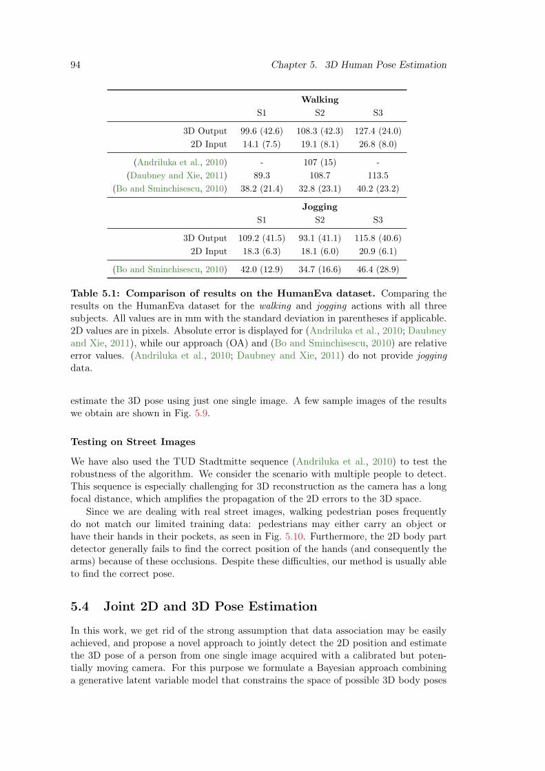
94 Chapter 5. 3D Human Pose Estimation
Walking
S1 S2 S3
3D Output 99.6 (42.6) 108.3 (42.3) 127.4 (24.0)
2D Input 14.1 (7.5) 19.1 (8.1) 26.8 (8.0)
(Andriluka et al., 2010) - 107 (15) -
(Daubney and Xie, 2011) 89.3 108.7 113.5
(Bo and Sminchisescu, 2010) 38.2 (21.4) 32.8 (23.1) 40.2 (23.2)
Jogging
S1 S2 S3
3D Output 109.2 (41.5) 93.1 (41.1) 115.8 (40.6)
2D Input 18.3 (6.3) 18.1 (6.0) 20.9 (6.1)
(Bo and Sminchisescu, 2010) 42.0 (12.9) 34.7 (16.6) 46.4 (28.9)
Table 5.1: Comparison of results on the HumanEva dataset. Comparing theresults on the HumanEva dataset for the walking and jogging actions with all threesubjects. All values are in mm with the standard deviation in parentheses if applicable.2D values are in pixels. Absolute error is displayed for (Andriluka et al., 2010; Daubneyand Xie, 2011), while our approach (OA) and (Bo and Sminchisescu, 2010) are relativeerror values. (Andriluka et al., 2010; Daubney and Xie, 2011) do not provide joggingdata.
estimate the 3D pose using just one single image. A few sample images of the resultswe obtain are shown in Fig. 5.9.
Testing on Street Images
We have also used the TUD Stadtmitte sequence (Andriluka et al., 2010) to test therobustness of the algorithm. We consider the scenario with multiple people to detect.This sequence is especially challenging for 3D reconstruction as the camera has a longfocal distance, which amplifies the propagation of the 2D errors to the 3D space.
Since we are dealing with real street images, walking pedestrian poses frequentlydo not match our limited training data: pedestrians may either carry an object orhave their hands in their pockets, as seen in Fig. 5.10. Furthermore, the 2D body partdetector generally fails to find the correct position of the hands (and consequently thearms) because of these occlusions. Despite these difficulties, our method is usually ableto find the correct pose.
5.4 Joint 2D and 3D Pose Estimation
In this work, we get rid of the strong assumption that data association may be easilyachieved, and propose a novel approach to jointly detect the 2D position and estimatethe 3D pose of a person from one single image acquired with a calibrated but poten-tially moving camera. For this purpose we formulate a Bayesian approach combininga generative latent variable model that constrains the space of possible 3D body poses

5.4. Joint 2D and 3D Pose Estimation 95
Ground Truth Part Detection Opt. PCA Best Reconst. Best Error Ours
−2000
−1000
0
1000500 1000
−500
0
500
1000
1500
−2000
−1000
0
1000500 1000
−500
0
500
1000
1500
−2000
−1000
0
1000500 1000
−500
0
500
1000
1500
−2000
−1000
0
1000500 1000
−500
0
500
1000
1500
S1, Walk, Frame 280 Err: 9.8± 5.3 px Err: 24.8mm Err: 46.6mm Err: 805.0mm Err: 55.3mm
−1000−800
−600−400
−200−100 0100200
0
200
400
600
800
1000
1200
1400
1600
−1000−800
−600−400
−200−100 0100200
0
200
400
600
800
1000
1200
1400
1600
−1000−800
−600−400
−200−100 0100200
0
200
400
600
800
1000
1200
1400
1600
−1000−800
−600−400
−200−100 0100200
0
200
400
600
800
1000
1200
1400
1600
S2, Walk, Frame 20 Err: 13.7± 5.2 px Err: 22.1mm Err: 102.4mm Err: 284.5mm Err: 102.4mm
−600−400
−200−1000−500
200
400
600
800
1000
1200
1400
1600
−600−400
−200−1000−500
200
400
600
800
1000
1200
1400
1600
−600−400
−200−1000−500
200
400
600
800
1000
1200
1400
1600
−600−400
−200−1000−500
200
400
600
800
1000
1200
1400
1600
S2, Jog, Frame 155 Err: 13.0± 8.8 px Err: 15.4mm Err: 68.8mm Err: 157.3mm Err: 68.8mm
600800
1000−1000−500
200
400
600
800
1000
1200
1400
1600
1800
600800
1000−1000−500
200
400
600
800
1000
1200
1400
1600
1800
600800
1000−1000−500
200
400
600
800
1000
1200
1400
1600
1800
600800
1000−1000−500
200
400
600
800
1000
1200
1400
1600
1800
S3, Jog, Frame 280 Err: 17.5± 13.0 px Err: 26.3mm Err: 72.6mm Err: 105.3mm Err: 89.5mm
Figure 5.9: 3D Human Pose Estimation Results. Leftmost two columns: Rawimage with 2D ground truth projection, and the 2D detection results with the associ-ated average pixel distance from ground truth. Rightmost four columns: Opt. PCA:projection of the ground truth on the PCA; Best Reconstruction: the sample with low-est reconstruction error; Best Error: the sample with the lowest error εlr (consistingof reprojection error and limb length errors); and Ours: the solution obtained. Beloweach solution we indicate the corresponding reconstruction error (in mm). Note thatminimizing εlr does not guarantee retrieving a good solution.
with a HOG-based discriminative model that constrains the 2D location of the bodyparts. The two models are simultaneously updated using an evolutionary strategy. Inthis manner 3D constraints are used to update image evidence while 2D observationsare used to update the 3D pose. As shown in Fig. 5.11 these strong ties make it pos-sible to accurately detect and estimate the 3D pose even when image evidence is verypoor.
Method
Figure 5.12 shows an overview of our model for simultaneous 2D people detection and3D pose estimation. It consists of two main components: a 3D generative kinematicmodel, which generates pose hypotheses, and a discriminative part model, which weights

96 Chapter 5. 3D Human Pose EstimationFra
me
7045
−500
0
500
−1500−1000−50005001000
200
400
600
800
1000
1200
1400
1600
Fra
me
7141
01000
20003000
−50005001000150020002500
500
1000
1500
Figure 5.10: Results on the TUD Stadtmitte sequence. Left three columns: Rawinput image, followed by the detected Gaussians and the reprojection of the estimated3D pose on the scene. Right column: Estimated 3D pose.
Raw 2D with Detectors 3D Output Example Result
Figure 5.11: Simultaneous estimation of 2D and 3D pose. First column: Rawinput image. Second column: Ground truth 2D pose (green) and the result of ourapproach (red). Additionally, we plot a few part detectors and their correspondingscore, used to estimate 3D pose. Reddish areas represent regions with highest responses.Third column: 3D view of the resulting pose. Note that despite the detectors notbeing very precise, our generative model allows estimating a pose very close to theactual solution. Last Column: We show an example of a challenging scene with severalpedestrians.
the hypotheses based on image appearance. Drawing inspiration from the approachproposed in (Andriluka et al., 2009) for 2D articulated shapes, we represent this modelusing a Bayesian formulation.
With this purpose, we represent 3D poses as a set of N connected parts. Letl = {l1, . . . , lN} be their 2D configuration with li = (ui, vi, si). (ui, vi) is the imageposition of the center of the part, and si a scale parameter which will be defined below.In addition let d = {d1, . . . ,dN} be the set of image evidence maps, i.e., the maps forevery part detector at different scales and for the whole image. Assuming conditional

5.4. Joint 2D and 3D Pose Estimation 97
...
+
Best Estimation Found
Use discriminative evidence to generate samples that are most likely
Sampling Projection
DISCRIMINATION BY 2D PART DETECTORSPROBABILISTIC GENERATIVE MODEL SAMPLING
hth
hu hl
hra hla hrl hll
h0
Figure 5.12: Overview of our method for simultaneous 2D and 3D pose esti-mation. Our approach consists of two main building blocks: a probabilistic generativemodel and a set of discriminative 2D part detectors. Our optimization framework si-multaneously solves for both the 2D and 3D pose using an evolutionary strategy. Aset of weighted samples are generated from the probabilistic generative model and aresubsequently reweighted by the score given by the 2D part detectors. This process isrepeated until convergence of the method. The rightmost figure shows results at con-vergence where the red shapes are the estimated poses and the green ones correspondto the ground truth.
independence of the evidence maps given l, and that the part map di only depends onli, the likelihood of the image evidence given a specific body configuration becomes:
p (d | l) =N∏
i=1
p (di | li) . (5.11)
In (Andriluka et al., 2009), Eq. (5.11) is further simplified under the assumptionthat the body configuration may be represented using a tree topology. This yields anadditional efficiency gain, as it introduces independence constraints between branches,e.g., the left arm/leg does not depend on the right arm/leg. Yet, this causes the issue ofthe double counting, where the same arm/leg is considered to be both the left and rightone. In (Andriluka et al., 2012) this is addressed by first solving an optimal tree andafterwards attempting to correct these artefacts using loopy belief propagation. Insteadof using two stages, we directly represent our 3D model using a Directed Acyclic Graph,which enforces anthropomorphic constraints, and helps preventing the double countingproblem.
Let x = {p1, . . . ,pN} be the 3D model that projects on the 2D pose l, where pi =(xi, yi, zi) is the 3D position of i-th part center. We write the posterior of x given theimage evidence d by:
p (x | d) ∝N∏
i=1
(p (di | li) p (li | pi)) p (x) .
In order to handle the complexity of directly modeling p (x), we propose approxi-mating x through a generative model based on latent variables h. This allows us tofinally write the problem as:
p (x | d) ∝ p (h) p (x | h)︸ ︷︷ ︸
generative
N∏
i=1
(p (di | li) p (li | pi))
︸ ︷︷ ︸
discriminative

98 Chapter 5. 3D Human Pose Estimation
Octave 1 4 7 10 13 16 19 22 25 28 31
Hea
dLef
tH
and
Lef
tFoot
Figure 5.13: 2D Part Detectors. We visualize the response at different octaves forthree different part detectors. We overlay the projection of the 3D ground truth in whiteto get an idea of the accuracy. The outputs are normalized for visualization purposes,with the dark blue and bright red areas corresponding to lower and higher responsesrespectively. Note that while some detectors, such as the head one in the first row,generally give good results, others do not, such as the left hand detector in the middlerow. Our approach can handle these issues by combining these 2D part detectors witha generative model.
where the discriminative and generative components become clearly separated. We willnext describe each of these components.
Discriminative Detectors
Recent literature proposes two principal alternatives for discriminative detectors: theshape context descriptors built by applying boosting on the limbs (Andriluka et al.,2009), and the HOG template matching approach (Yang and Ramanan, 2011). Forour purposes we have found the HOG-based template matching to be more adequatebecause it matches our joint-based 3D model better as we can place a detector at eachjoint part instead of having to infer the limb positions from the joints. In addition,the HOG template matching yields smoother responses, which is preferable when doinginference.
As mentioned above, each part li has an associated scale parameter si. This pa-rameter is used to pick a specific scale among the evidence maps. Intuitively, if a partis far away, it should be evaluated by a detector at a small scale (high resolution). Wetherefore approximate the scale si as:
s−1i = α−1βzi (5.12)

5.4. Joint 2D and 3D Pose Estimation 99
where α is the focal length of the camera and is used for normalization purposes. Theparameter β will be learned off-line and used during inference. Note that despite thisparameter constant, the scale at which each part is evaluated is different as it dependson the zi coordinate.
Let t = {t1, . . . , tN} be the set of templates in the HOG space associated to eachbody part. These templates are provided in (Yang and Ramanan, 2011)1. Given abody part li, its image evidence di is computed by evaluating the template ti overthe entire image for a range of scales si. Figure 5.13 illustrates the response of threepart detectors at different scales. By interpreting each detector as a log-likelihood, theimage evidence of a configuration L can be computed as:
log p (l | d) ≈ score(l) =N∑
i=1
kidi(ui, vi, si) , (5.13)
where ki is a weight associated to each detector, which is learned offline. It is meantto adapt the 2D detectors and 3D generative model due to the fact they were trainedindependently on different datasets.
Additionally, when evaluating a part detector at a point, we consider a small windowfrom which we use the largest detector value in order to give additional noise toleranceto the detector. We find this necessary as small 2D errors can have large consequencesin 3D positioning.
Latent Generative Model
We use the Directed Acyclic Graph model explained in Section 4.4. This model dis-creticizes the poses to be able to learn the joint distribution of the 3D poses and alatent space by using Expectation Maximization. Given that the model does not con-tain loops, efficient inference can be done using dynamic programming. This allows themodel to be used in a generative fashion in which the latent space is sampled and thenthe most likely 3D pose for the latent space configuration is efficiently estimated.
Inference
The inference problem consists of computing:
<X∗>= argmaxx
N∏
i=1
(p (di | li) p (li | pi)) p (x | h) p (h) . (5.14)
We treat this as a global optimization problem where, given a set of 2D detectionscorresponding to the different parts from a single image, we optimize over both a rigidtransformation and the latent states. Drawing inspiration in (Moreno-Noguer andFua, 2013; Moreno-Noguer et al., 2010), we do this using a variation of the CovarianceMatrix Adaptation Evolutionary Strategy (CMA-ES) (Hansen, 2006), which is a blackbox global optimizer that uses a Gaussian distribution in the search space to minimize
1Indeed, each of the part detectors provided in (Yang and Ramanan, 2011) is formed by severaltemplates and we use their maximum score for each coordinate (u, v, s). For ease of explanation werefer to them as a single template.

100 Chapter 5. 3D Human Pose Estimation
(Yang and Ramanan, 2011) Ideal Detector Our Approach
Err. 2D 2D 3D Pose 2D 3D Pose
All 21.7 11.0 106.6 51.6 19.5 237.3 55.3
C1 19.5 11.1 113.8 52.3 18.9 239.1 55.2
C2 22.9 11.1 109.7 51.2 19.6 245.8 55.4
C3 22.8 10.8 96.2 51.2 20.0 227.1 55.4
S1 21.8 10.2 96.8 63.4 19.9 277.2 69.3
S2 21.8 10.8 108.0 44.8 18.6 206.6 46.8
S3 21.6 12.3 119.0 43.7 20.1 221.4 46.6
A1 20.9 10.7 106.0 56.2 19.3 254.4 60.3
A2 22.7 11.3 107.2 46.6 19.7 219.0 50.0
Table 5.2: Results on the HumanEva dataset. We show results for the walking(A1) and jogging (A2) actions with all subjects (S1,S2,S3) and cameras (C1,C2,C3).We compare with the 2D error obtained using the 2D model from (Yang and Ramanan,2011), based on the same part detectors we use. 2D, 3D and Pose Errors are definedin the text. Ideal detector corresponds to our approach using Gaussians with 20pxcovariance as 2D input instead of the 2D detections.
a function. In our case we perform:
argmaxR,t,H
score
(
projR,t
(φ−1 (h)
)
)
+ log(p(φ−1 (h) ,h
)),
where projR,t(·) is the result of applying a rotation R, a translation t and projectingonto the image plane. We then take x∗=Rφ−1(h∗) + t, that is, we obtain the mostprobable xL∗ given h∗ and perform a rigid transformation to the world coordinates toobtain x∗.
Results
We numerically evaluate our algorithm on the HumanEva benchmark (Sigal et al.,2010b), which provides 3D ground truth for various actions. In addition, we providequalitative results on the TUD Stadtmitte sequence (Andriluka et al., 2010), a clutteredstreet sequence. For both cases, we compute the 2D observations using the detectorsfrom (Yang and Ramanan, 2011) trained independently on the PARSE dataset (Ra-manan, 2006).
We consider three error metrics: 2D error, 3D error and 3D pose error. The 2Derror measures the mean pixel difference between the 2D projection of the estimated3D shape, and the ground truth. 3D error is the mean euclidean distance, in mm, withthe ground truth, and the 3D pose error is the mean euclidean distance with the groundtruth after performing a rigid alignment of the two shapes. This error is indicative ofthe local deformation error. We evaluate three times on every 5 images using all threecameras and all three subjects for both the walking and jogging actions, for a total of1318 unique images.
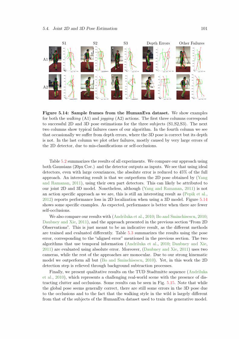
5.4. Joint 2D and 3D Pose Estimation 101
S1 S2 S3 Depth Errors Other Failures
A1
−4000−3800−3600
−1100−1000
−900−800−700
−800
−600
−400
−200
0
200
400
600
−3700−3600−3500−3400−3300
−400−200
0
−800
−600
−400
−200
0
200
400
600
−4400−4200−4000
−1000−800
−600
−800
−600
−400
−200
0
200
400
600
−3600−3400−3200−3000
−400−200
0
−800
−600
−400
−200
0
200
400
−5200−5000−4800
0200
400
−600
−400
−200
0
200
400
600
800
A2
−3900−3800−3700−3600−3500
400600
800
−800
−600
−400
−200
0
200
400
600
−3800−3600−3400
−800−600
−400
−800
−600
−400
−200
0
200
400
−3500−3400−3300−3200−3100
400600
−800
−600
−400
−200
0
200
400
600
−3200−3000−2800
−1000
100200300
−800
−600
−400
−200
0
200
400
−3800−3600−3400
−600−400
−200
−800
−600
−400
−200
0
200
400
600
Figure 5.14: Sample frames from the HumanEva dataset. We show examplesfor both the walking (A1) and jogging (A2) actions. The first three columns correspondto successful 2D and 3D pose estimations for the three subjects (S1,S2,S3). The nexttwo columns show typical failures cases of our algorithm. In the fourth column we seethat occasionally we suffer from depth errors, where the 3D pose is correct but its depthis not. In the last column we plot other failures, mostly caused by very large errors ofthe 2D detector, due to mis-classifications or self-occlusions.
Table 5.2 summarizes the results of all experiments. We compare our approach usingboth Gaussians (20px Cov.) and the detector outputs as inputs. We see that using idealdetectors, even with large covariances, the absolute error is reduced to 45% of the fullapproach. An interesting result is that we outperform the 2D pose obtained by (Yangand Ramanan, 2011), using their own part detectors. This can likely be attributed toour joint 2D and 3D model. Nonetheless, although (Yang and Ramanan, 2011) is notan action specific approach as we are, this is still an interesting result as (Pepik et al.,2012) reports performance loss in 2D localization when using a 3D model. Figure 5.14shows some specific examples. As expected, performance is better when there are fewerself-occlusions.
We also compare our results with (Andriluka et al., 2010; Bo and Sminchisescu, 2010;Daubney and Xie, 2011), and the approach presented in the previous section “From 2DObservations”. This is just meant to be an indicative result, as the different methodsare trained and evaluated differently. Table 5.3 summarizes the results using the poseerror, corresponding to the “aligned error” mentioned in the previous section. The twoalgorithms that use temporal information (Andriluka et al., 2010; Daubney and Xie,2011) are evaluated using absolute error. Moreover, (Daubney and Xie, 2011) uses twocameras, while the rest of the approaches are monocular. Due to our strong kinematicmodel we outperform all but (Bo and Sminchisescu, 2010). Yet, in this work the 2Ddetection step is relieved through background subtraction processes.
Finally, we present qualitative results on the TUD Stadtmitte sequence (Andrilukaet al., 2010), which represents a challenging real-world scene with the presence of dis-tracting clutter and occlusions. Some results can be seen in Fig. 5.15. Note that whilethe global pose seems generally correct, there are still some errors in the 3D pose dueto the occlusions and to the fact that the walking style in the wild is largely differentfrom that of the subjects of the HumanEva dataset used to train the generative model.

102 Chapter 5. 3D Human Pose Estimation
Walking (A1,C1)
S1 S2 S3
Joint 2D and 3D 65.1 (17.4) 48.6 (29.0) 73.5 (21.4)
From 2D Observations 99.6 (42.6) 108.3 (42.3) 127.4 (24.0)
(Daubney and Xie, 2011) 89.3 108.7 113.5
(Andriluka et al., 2010) - 107 (15) -
(Bo and Sminchisescu, 2010) 38.2 (21.4) 32.8 (23.1) 40.2 (23.2)
Jogging (A2,C1)
S1 S2 S3
Joint 2D and 3D 74.2 (22.3) 46.6 (24.7) 32.2 (17.5)
From 2D Observations 109.2 (41.5) 93.1 (41.1) 115.8 (40.6)
(Bo and Sminchisescu, 2010) 42.0 (12.9) 34.7 (16.6) 46.4 (28.9)
Table 5.3: Comparison against state-of-the-art approaches. We present resultsfor both the walking and jogging actions for all three subjects and camera C1. From2D Observations refers to the first approach presented in this chapter.
Frame 7056 Frame 7126
Figure 5.15: Two sample frames from the TUD Stadtmitte sequence (An-driluka et al., 2010).
5.5 Summary
We have presented two different approaches for 3D human pose estimation from singlemonocular images. This is an extremely challenging problem as it is severely under-constrained. Despite the difficulty we have been able to obtain very promising resultswith both approaches, each with a different set of strengths and weaknesses.
In the first approach a 2D pose estimation model is used to initially obtain a noisyobservation that can be used for 3D pose estimation. The method consists of a linearprojection model that constrains the possible 3D positions given the 2D observations incombination with a linear latent model for the 3D pose. By fusing both linear models,we are able to obtain a linear formulation of the camera constraints on the latent space.This allows a noisy 2D pose estimation to be projected to the 3D pose space in which ahypergaussian is obtained. Afterwards anthropomorphism is used as a criteria to discernthe most realistic pose obtained from sampling from the hypotheses. The advantage ofthis formulation is in its simplicity, which allows it to be very computationally efficient,

5.5. Summary 103
limited only by the speed of the 2D pose estimation model. However, by being apipelined approach, the quality of the 3D output is limited by that of the 2D input.
For our second approach we employ 2D discriminative detectors directly as the modelinput and then perform 2D and 3D pose estimation jointly. This is done by extendingthe Bayesian formulation of pictorial structures to 3D and reformulating it as a hybridgenerative-discriminative model. For the generative model we use a Directed AcyclicGraph, which allows probabilistic representing 3D human poses through a discrete latentspace. The discriminative model consists of reweighting 2D detectors for the 3D humanpose estimation task. We treat the inference as a global optimization problem andsolve it iteratively using state-of-the-art techniques. By performing 2D and 3D poseestimation jointly, the 3D is able to correct errors caused by occlusions in the 2Ddetections.
Our findings with both approaches show that it is indeed possible to obtain good 3Dhuman pose estimation results despite the complexity of the problem. This is done byleveraging the prior knowledge of human motion with generative models. Stronger priorsallow much more accurate pose estimation by eliminating non-realistic pose hypotheses.We are also able to see that performing 2D and 3D pose estimation jointly is beneficialto performance. By delaying the pose estimation decision to the end and leveraging allthe available information, the noise in the 2D part detectors is minimized.
In the next chapter we will show that the output of pose estimators can be used tocreate strong features when performing higher order reasoning.


Chapter 6
Probabilistically Modelling Fashion
The finest clothing made is aperson’s skin, but, of course,society demands something morethan this.
Mark Twain
In this chapter we will discuss higher level computer vision tasks in a fashion context.These high level task push the boundaries of what is possible with modern computervision and machine learning, while being the contributions that are able to influencepeople in their daily life.
In particular we shall focus on two tasks: semantic segmentation of clothings infashion photographs, and prediction of fashionability while providing fashion advice.The first task is based on a standard problem in computer vision, however, the appli-cation domain is vastly different. In particular the large number of classes with highintra-class variability in combination with the fine-grained level of annotations make itan extremely challenging problem. In our second task we tackle the novel problem ofpredicting fashionability of an individual in an image with some associated metadata.We also take it a step further and attempt to give advice to the user on which outfitswould suit her/him better.
All the work in this chapter is a result of collaborating with Prof. Raquel Urtasunand Prof. Sanja Fidler, from the University of Toronto.
6.1 Introduction
Fashion has a tremendous impact on our society. Clothing typically reflects the person’ssocial status and thus puts pressure on how to dress to fit a particular occasion. Itsimportance becomes even more pronounced due to online social sites like Facebookand Instagram where one’s photographs are shared with the world. We also live ina technological era where a significant portion of the population looks for their dreampartner on online dating sites. People want to look good; business or casual, elegant
105

106 Chapter 6. Probabilistically Modelling Fashion
Input Truth (Yamaguchi et al., 2012) Ours
Figure 6.1: Garment segmentation example. We show our approach in a scenariowhere no a priori knowledge of which garments are worn is provided. We compareagainst state-of-the-art. Despite some mistakes, our result looks visually much morenatural than the competing method.
or sporty, sexy but not slutty, and of course trendy, particularly so when putting theirpicture online. This is reflected in the growing online retail sales, reaching 370 billiondollars in the US by 2017, and 191 billion euros in Europe (Forbes Magazine, 2013).
Computer vision researchers have started to be interested in the subject due tothe high impact of the application domain (Bossard et al., 2012; Bourdev et al., 2011;Chen et al., 2012; Gallagher and Chen, 2008; Hasan and Hogg, 2010; Jammalamadakaet al., 2013; Liu et al., 2012b; Wang and Ai, 2011). The main focus has been to inferclothing from photographs. This can enable a variety of applications such as virtualgarments in online shopping. Being able to automatically parse clothing is also keyin order to conduct large-scale sociological studies related to family income or urbangroups (Murillo et al., 2012; Song et al., 2011).
In the context of fashion, Yamaguchi et al. (Yamaguchi et al., 2012), created Fash-ionista, a dataset of images and clothing segmentation labels. Great performance wasobtained when the system was given information about which garment classes, but nottheir location, are present for each test image. Unfortunately, the performance of thestate-of-the-art methods (Yamaguchi et al., 2012; Jammalamadaka et al., 2013) is ratherpoor when this kind of information is not provided at test time. This has been veryrecently partially addressed in (Yamaguchi et al., 2013) by utilizing over 300,000 weaklylabeled images, where the weak annotations are in the form of image-level tags. Inthis chapter, we show an approach which outperforms the state-of-the-art significantlywithout requiring these additional annotations, by exploiting the specific domain of thetask: clothing a person. An example of our result can be seen in Fig. 6.1.
In this chapter we also present a second task in which our goal is to predict howfashionable a person looks on a particular photograph. The fashionability is affected bythe garments the subject is wearing, but also by a large number of other factors such ashow appealing the scene behind the person is, how the image was taken, how visuallyappealing the person is, her/his age, etc. The garment itself being fashionable is alsonot a perfect indicator of someone’s fashionability as people typically also judge howwell the garments align with someone’s “look”, body characteristics, or even personality.

6.2. Segmentation of Garments in Fashion Images 107
background heels blazer stockings blouse hat
hair wedges cardigan tights top purse
skin shoes jumper shorts skirt belt
Figure 6.2: Fine-grained annotations of the Fashionista dataset (Yamaguchiet al., 2012). Many of the different classes are very difficult to distinguish even forhumans. Observe the subtle differences between some classes such as footwear (heels,wedges, and shoes), blazer and cardigan, or stockings and tights. We also point out thatthis dataset has been annotated via superpixels, and thus the ground truth containserrors when superpixels do not align with the actual garments. We have not modifiedthe ground truth segmentation in any way.
6.2 Segmentation of Garments in Fashion Images
The complexity of the task of human semantic segmentation comes from the inherentvariability of pose and cloth appearances, the presence of self-occlusions as well as thepotentially large number of classes. Consider for example Fig. 6.2: an autonomoussystem needs to distinguish between blazers and cardigans, stockings and tights, andheels, wedges and shoes, where the intra-class variability is fundamentally much largerthan the inter-class variability. This fine-grained categorization is difficult to resolveeven for humans who are not familiar with the fashion industry. The problem is furtheraggravated by the power law distribution of classes, as certain categories have very fewexamples. Thus, extra-care has to be taken into account to not over-predict the classesthat are very likely to appear in each image, e.g., skin, hair.
In this section we address some of these challenges and formulate the problem asthe one of inference in a Conditional Random Field (CRF), which takes into accountthe complex dependencies between clothing and human pose. Specifically, we developa rich set of potentials which encode the person’s global appearance and shape toperform figure/ground segmentation, shape and location likelihoods for each garment,which we call clothelets, and long-range similarity between segments to encourage, forexample, T-Shirt pixels on the body to agree with the T-shirt pixels on the person’sarm. We further exploit the fact the people are symmetric and dress as such as wellby introducing symmetry-based potentials between different limbs. We also use a va-riety of different local features encoding cloth appearance as well as local shape of theperson’s parts. We demonstrate the effectiveness of our approach on the Fashionistadataset (Yamaguchi et al., 2012) and show that our approach significantly outperformsthe existing state-of-the-art.

108 Chapter 6. Probabilistically Modelling Fashion
Related Work
There has been a growing interest in recognizing outfits and clothing from still images.One of the first approaches on the subject was Chen et al. (Chen et al., 2006), whichmanually built a composite clothing model, that was then matched to input images.This has led to more recent applications for learning semantic clothing attributes (Chenet al., 2012), which are in turn used for describing and recognizing the identity of individ-uals (Bourdev et al., 2011; Gallagher and Chen, 2008), their style (Bossard et al., 2012),and performing sociological studies such as predicting the occupation (Song et al., 2011)or urban tribes (Murillo et al., 2012). Other tasks like outfit recommendations (Liuet al., 2012a) have also been investigated. However, in general, these approaches donot perform accurate segmentation of clothing, which is the goal of our approach. In-stead, they rely on more coarse features such as bounding boxes and focus on producinggeneric outputs based on the presence/absence of a specific type of outfit. It is likelythat the performance of such systems would improve if accurate clothing segmentationwould be possible.
Recent advances in 2D pose estimation (Bourdev and Malik, 2009; Yang and Ra-manan, 2011) have enabled a more advanced segmentation of humans (Dong et al.,2013). However, most approaches have focused on figure/ground labeling (Ladickyet al., 2013; Wang and Koller, 2011). Additionally, pose information has been used asa feature in clothing related tasks such as finding similar worn outfits in the context ofonline shopping (Liu et al., 2012b).
Segmentation and classification of garments has been addressed in the restrictivecase in which the labels are known beforehand (Yamaguchi et al., 2012). The originalpaper tackled this problem in the context of fashion photographs which depicted oneperson typically in an upright pose. This scenario has also been extended to the casewhere more than one individual can be present in the image (Jammalamadaka et al.,2013). In order to perform the segmentation, conditional random fields are used withpotentials linking clothing and pose. However, the performance of these approachesdrops significantly when no information about the outfit is known a priori (i.e., notags are provided at test time). The paper doll approach (Yamaguchi et al., 2013) usesover 300,000 weakly labeled training images and a small set of fully labeled examplesin order to enrich the model of (Yamaguchi et al., 2012) with a prior over image labels.As we will show in the experimental evaluation, our method can handle this scenariowithout having to resort to additional training images. Furthermore, it consistentlyoutperforms (Yamaguchi et al., 2012, 2013).
CRFs have been very successful in semantic segmentation tasks. Most approachescombine detection and segmentation by using detectors as additional image evidence (Yaoet al., 2012b; Fidler et al., 2013). Co-occurrence potentials have been employed to en-force consistency among region labels (Ladicky et al., 2010). Part-based detectors havealso been aligned to image contours to aid in object segmentation (Brox et al., 2011).All these strategies have been applied to generic segmentation problems, where one isinterested in segmenting classes such as car, sky or trees. Pixel-wise labeling of clothingis, however, a much more concrete task, where strong domain specific information, suchas 2D body pose, can be used to reduce ambiguities.

6.2. Segmentation of Garments in Fashion Images 109
Type Name Description
unary Simple features (φsimplei,j (yi)) Assortment of simple features.
unary Object mask (φobji,j (yi)) Figure/ground segmentation ask.
unary Clothelets (φclothi,j (yi)) Pose-conditioned garment likelihood masks.
unary Ranking (φo2pi,j (yi)) Rich set of region ranking features.
unary Bias (φbiasj (yi) and φbiasp,j (lp)) Class biases.
pairwise Similarity (φsimilm,n (ym, yn)) Similarity between superpixels.
pairwise Compatibility (φcompi,p (yi, lp)) Edges between limb segments and superpixels.
Table 6.1: Overview of the different types of potentials used in the proposedCRF model.
Clothing a Person
Our proposed Conditional Random Field (CRF) takes into account complex dependen-cies that exist between garments and human pose. We obtain pose by employing a 2Darticulated model by Yang et al. (Yang and Ramanan, 2011) which predicts the mainkeypoints such as head, shoulders, knees, etc. As (Yamaguchi et al., 2012), we willexploit these keypoints to bias the clothing labeling in a plausible way (e.g., a hat istypically on the head and not the feet). To manage the complexity of the segmentationproblem we represent each input image with a small number of superpixels (P.Arbe-laez et al., 2011). Our CRF contains a variable encoding the garment class (includingbackground) for each superpixel. We also add limb variables which encode the garmentassociated with a limb in the human body and correspond to edges in the 2D articulatedmodel. We use the limb variables to propagate information while being computationallyefficient.
Our CRF contains a rich set of potentials which exploit the domain of the task. Weuse the person’s global appearance and shape to perform figure/ground segmentationin order to narrow down the scope of cloth labeling. We further use shape and locationlikelihoods for each garment, which we call clothelets. We exploit the fact that peopleare symmetric and typically dress as such by forming long-range consistency potentialsbetween detected symmetric keypoints of the human pose. We finally also use a varietyof different features that encode appearance as well as local shape of superpixels.
We will now discuss the different potentials in the model. All our potentials belongto the exponential function family, however, for notation simplicity we will write thelogarithm of the potentials and not make explicit the dependency with the observedvariables.
Pose-aware Model
Given an input image represented with superpixels, our goal is to assign a clothing label(or background) to each of them.
More formally, let yi ∈ {1, · · · , C} be the class associated with the i-th superpixel,and let lp be the p-th limb segment defined by the edges in the articulated body model.Each limb lp is assumed to belong to one class, lp ∈ {1, · · · , C}. To encode bodysymmetries in an efficient manner, we share limb variables between the left and right

110 Chapter 6. Probabilistically Modelling Fashion
Image Person Mask Limbs Image Person Mask Limbs
Figure 6.3: Visualization of object masks (Carreira and Sminchisescu, 2012)and limbs (obtained via (Yang and Ramanan, 2011)). Note that CPMC typicallygenerates high quality results, e.g. the one in the left image, but can also completelymiss large parts of the body as shown in the image on the right.
part of the human body, e.g., the left and the right leg share the same limb variables.We propose several domain inspired potentials, the overview of which is presented inTable 6.1. We emphasize that the weights associated with each potential in our CRFwill be learned using structure prediction. We now explain each potential in more detail.
Simple Features: Following (Yamaguchi et al., 2012), we concatenate a diverse setof simple local features and train a logistic regression classifier for each class. In par-ticular, we use colour features, normalized histograms of RGB and CIE L*a*b* colour;texture features, Gabor filter responses; and location features: both normalized 2D im-age coordinates and pose-relative coordinates. The output of the logistic functions arethen used as unary features in the CRF. This results in a unary potential with as manydimensions as classes:
φsimplei,j (yi) =
{
wsimplej σsimplej (fi), if yi = j
0, otherwise, (6.1)
where wsimplej is the weight for class j, σsimplej (fi) is the score of the classifier for classj, and fi is the concatenation of all the features for superpixel i. Notice we have usedC different unary potentials, one for each class. By doing this, we allow the weights ofa variety of potentials and classes be jointly learned within the model.
Figure/Ground Segmentation: To facilitate clothing parsing we additionally com-pute how likely it is that each superpixel belongs to a person. We do this by com-puting a set of bottom-up region proposals using the Constrained Parametric Min-Cuts(CPMC) approach (Carreira and Sminchisescu, 2012), which repetitively solves a fig-ure/ground energy minimization problem with different parameters and seeds via para-metric min-cuts. We take top K (we set K = 100) regions per image and use Order 2Pooling (O2P) (Carreira et al., 2012) to score each region into figure/ground (person-vs-background). Since we know that there is a person in each image, we take at leastthe top scoring segment per image, no matter its score. For images with multiple highscoring segments, we take the union of all segments with scores higher than a learnedthreshold (Carreira et al., 2012). We define a unary potential to encourage the super-pixels that lie inside the foreground mask to take any of the clothing labels (and not

6.2. Segmentation of Garments in Fashion Images 111
Image Background Skin Socks Jacket Bag
Figure 6.4: Visualization of clothelets. We show several clothelets for two differentinput images.
background):
φobji,j (yi) =
{
wcmpc1 σcpmc · |¬Mfg ∩ Si|/|Si|, if yi = 1
wcpmcj σcpmc · |Mfg ∩ Si|/|Si|, otherwise, (6.2)
where yi = 1 encodes the background class, wcpmcj is the weight for class j, σcpmc is thescore of the foreground region, Si, Mfg are binary masks defining the superpixel andforeground, respectively, and ¬Mfg is a mask of all pixels not in foreground. Fig. 6.3shows examples of masks obtained by (Carreira et al., 2012). Note that while in somecases it produces very accurate results, in others, it performs poorly. These inaccuratemasks are compensated by other potentials.
Clothelets: Our next potential exploits the statistical dependency between the loca-tion on the human body and garment type. Its goal is to make use of the fact thate.g. jeans typically cover the legs and not the head. We compute a likelihood of eachgarment appearing in a particular relative location of the human pose. In particular,for each training example we take a region around the location of each joint (and limb),the size of which corresponds to the size of the joint part template encoded in (Yangand Ramanan, 2011). We average the GT segmentation masks for each class across thetraining examples. In order to capture garment classes that stray away from the pose,we use boxes that are larger than the part templates in (Yang and Ramanan, 2011).At test time, the masks for each class are overlaid relative to the inferred pose and nor-malized by the number of non-zero elements. Areas with no information are assignedto the background class. The potential is then defined as
φclothi,j (yi) =
{
wclothj (clotheletji · Si)/|Si|, if yi = j
0, otherwise, (6.3)

112 Chapter 6. Probabilistically Modelling Fashion
where wclothj is the weight for class j, clotheletji is the clothelet for the j-th class, and ·is the dot product. Fig. 6.4 depicts clothelets for a few sample classes. Note that theselikelihoods are conditioned on the pose.
Shape Features: This potential uses a set of rich features that exploit both the shapeand local appearance of garments. In particular, we use eSIFT and eMSIFT proposedby (Carreira et al., 2012) for region description. Given a region, both descriptors extractSIFT inside the region and enrich it with the relative location and scale within theregion. Second-order pooling is used to define the final region descriptor. eSIFT andeMSIFT differ slightly in how the descriptors are pooled, eSIFT pools over both theregion and background of the region, while eMSIFT pools over the region alone.
While (Carreira et al., 2012) defines the features over full object proposals, herewe compute them over each superpixel. As such, they capture more local shape of thepart/limb and local appearance of the garment. We train a logistic classifier for eachtype of feature and class and use the output as our potential:
φo2pi,j (yi) =
{
wo2pj σo2pj (ri), if yi = j
0, otherwise, (6.4)
with wo2pj is the weight for class j, σo2pj (ri) the classifier score for class j, and ri thefeature vector for superpixel i.
Bias: We use a simple bias for the background to encode the fact that it is the classthat appears more frequently. Learning a weight for this bias is equivalent to learninga threshold for the foreground, however within the full model. Thus:
φbias(yi) =
{
wbias, if yi = 1
0, otherwise, (6.5)
where wbias is the single bias weight.
Similarity: In CRFs, neighboring superpixels are typically connected via a (contrast-sensitive) Potts model encouraging smoothness of the labels. For clothing parsing, wewant these connections to act on a longer range. That is, a jacket is typically split inmultiple disconnected segments due to a T-shirt, tie, and/or a bag. Our goal is to en-courage superpixels that are similar in appearance to agree on the label, even thoughthey may not be neighbors in the image.
We follow (Uijlings et al., 2013) and use size similarity, fit similarity that measureshow well two superpixels fit each other; and colour and texture similarity, with thetotal of 12 similarity features between each pair of superpixels. We then train a logisticregression to predict if two superpixels should have the same label or not. In order toavoid setting connections on the background, we only connect superpixels that overlapwith the bounding box of the 2D pose detection. Note that connecting all pairs ofsimilar superpixels would slow down inference considerably. To alleviate this problem,we compute the minimum spanning tree using the similarity matrix and use the top 10edges to connect 10 pairs of superpixels in each image. We form a pairwise potential

6.2. Segmentation of Garments in Fashion Images 113
between each connected pair:
φsimilm,n (ym, yn) =
{
wsimili σsimilm,n , if ym = yn = i
0, otherwise, (6.6)
where wsimili is the weight for class i, and σsimilm,n is the output of the similarity classifier.
Limb Segment Bias: We use a per-class bias on each limb segment to capture alocation specific bias, e.g., hat only appears in the head:
φbiasp,j (lp) =
{
wbiasp,j , if lp = j
0, otherwise, (6.7)
where wbiasp,j is a weight for part limb p and class j that allows us to compute whichclasses are more frequent in each limb.
Compatibility Segmentation-Limbs: We define potentials connecting limb seg-ments with nearby superpixels encouraging them to agree in their labels. Towards thisgoal, we first define a Gaussian mask centered between two joints. More formally, fortwo consecutive joints with coordinates Ja = (ua, va) and Jb = (ub, vb), we define themask based on the following Normal distribution:
M(Ja, Jb) = N
(
Ja + Jb2
, R
(
q1‖Ja − Jb‖ 0
0 q2
)
RT
)
, (6.8)
where R is a 2D rotation matrix with an angle arctan(ua−ubva−vb
), and q1 and q2 are twohyperparameters controlling the spread of the mask longitudinally and transversely,respectively. In order to additionally encode symmetry, a single limb segment is usedfor both left and right sides of the body, e.g., left and right shins will share the samekeypoint. The strength of the connection is based on the overlap between the superpixelsand the Gaussian mask:
φcompi,p (yi, lp) =
{
wcompj,p M(Ja, Jb) · Si, if yi 6= 1 and yi = kp = j
0, otherwise, (6.9)
where wcompi,p is the weight for part p and class j. For computational efficiency, edgeswith connection strengths below a threshold are not set in the model. Some examplesof the limb segment masks are shown in Fig. 6.3. We can see the masks fit the bodytightly to avoid overlapping with background superpixels.
Full Model: We define the energy of the full model to be the sum of three types ofenergies encoding unary and pairwise potentials that depend on the superpixel labeling,as well as an energy term linking the limb segments and the superpixels:
E(y, l) = Eunary(y) + Esimilarity(y) + Elimbs(y, l) . (6.10)
This energy is maximized during inference. The unary terms are formed by the concate-nation of appearance features, figure/ground segmentation, clothelets, shape features

114 Chapter 6. Probabilistically Modelling Fashion
0.3
0.4
0.5
0.6
0.7
0.8
0.9
1
Clothing classes Similarity (dlch)
jumper vs sweater 1.000
jumper vs sweatshirt 0.697
jumper vs top 0.557
jumper vs stockings 0.507
jumper vs heels 0.465
jumper vs sunglasses 0.341
jumper vs watch 0.317
Figure 6.5: Wordnet-based similarity function. We use the inverse of theLeacock-Chodorow Similarity between the classes in the Fashionista dataset to weighour loss function. We display the similarity matrix between all the classes on the left.Some individual values of the similarity between the jumper class and several otherclasses can be seen on the right.
and background bias for a total of K = (1 + 5C) features
Eunary(y) =N∑
i=1
K∑
j=1
φunaryi,j (yi) , (6.11)
where N is the number of superpixels. The pairwise features encode the similaritybetween different pairs of superpixels as we describe above
Esimilarity(y) =∑
(m,n)∈pairs
φsimilm,n (ym, yn) . (6.12)
The limb-superpixel compatibility term is defined as
Elimbs(y, l) =M∑
p=1
C∑
j=1
(
φbiasp,j (lp) +N∑
i=1
φcomp(yi, lp)
)
, (6.13)
for a total of (M + C) features, with M the number of limb segments.
Learning and Inference
Our model is a multi-label CRF which contains cycles and thus inference is NP-hard.We use a message passing algorithm, distributed convex belief propagation (Schwinget al., 2011) to perform inference. It belongs to the set of LP-relaxation approaches, andhas convergence guarantees. This is not the case in other message passing algorithmssuch as loopy-BP.
To learn the weights, we use the primal-dual method of (Hazan and Urtasun, 2010)(we use the implementation of (Schwing et al., 2012)), shown to be more efficient thanother structure prediction learning algorithms.
As loss-function, we use the semantic similarity between the different classes in orderto penalize mistakes between unrelated classes more than similar ones. We do this

6.2. Segmentation of Garments in Fashion Images 115
29 Classes 56 Classes
Method Y2012 Ours Y2012 Y2013 Ours
Jaccard index 12.32 20.52 7.22 9.22 12.28
Table 6.2: Comparison against the state-of-the-art. We compare on two differentdatasets: Fashionista v0.2 with 56 classes and Fashionista v0.3 with 29 classes, againstY2012 (Yamaguchi et al., 2012) and Y2013 (Yamaguchi et al., 2013).
via Wordnet (Miller, 1995), which is a large lexical database in which sets of cognitivesynonyms (synsets) are interlinked by means of semantic and lexical relationships. Wecan unambiguously identify each of the classes with a single synset, and then proceed tocalculate similarity scores between these synsets that represent the semantic similaritybetween the classes, in order to penalize mistakes with dissimilar classes more.
In particular, we choose the corpus-independent Leacock-Chodorow Similarity score.This score takes into account the shortest path length p between both synsets and themaximum depth of the taxonomy d at which they occur. It is defined as the relationship− log(p/2d). A visualization of the dissimilarity between all the classes in the datasetcan be seen in Fig. 6.5. We therefore define the loss-function as:
∆y(yi, y∗i ) =
{
0, if yi = y∗idlch(yi, y
∗i ), otherwise
(6.14)
with dlch(·, ·) being the inverse Leacock-Chodorow Similarity score between both classes.For the limb segments we use a 0-1 loss:
∆k(ki, k∗i ) =
{
0, if ki = k∗i1, otherwise
(6.15)
Experimental Evaluation
We evaluate our approach on both a the Fashionista dataset v0.3 (Yamaguchi et al.,2012), and the setting of (Yamaguchi et al., 2013) with the Fashionista dataset v0.2.Both datasets are taken from chictopia.com in which a single person appears wearinga diverse set of garments. The dataset provides both annotated superpixels as wellas 2D pose annotations. A set of evaluation metrics and the full source code of ap-proaches (Yamaguchi et al., 2012, 2013) are provided. Version 0.2 has 685 images andv0.3 has 700 images. Note that v0.3 is not a superset of v0.2.
We have modified the Fashionista v0.3 dataset in two ways. First we have com-pressed the original 54 classes into 29. This is due to the fact that many classes thatappear have very few occurrences. In fact, in the original dataset, 13 classes have 10or fewer examples and 6 classes have 3 or fewer instances. This means that when per-forming a random split of the samples into training and test subsets, there is a highprobability that some classes will only appear in one of the subsets. We therefore com-press the classes by considering both semantic similarity and the number of instances.
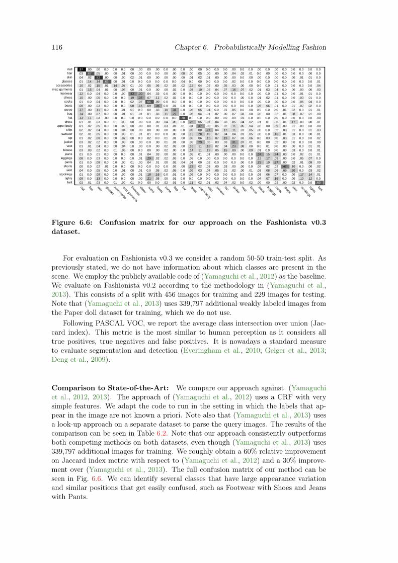
116 Chapter 6. Probabilistically Modelling Fashion
.97 .00 .00 0.0 0.0 0.0 .00 .00 .00 .00 0.0 .00 0.0 .00 .00 0.0 0.0 0.0 .00 0.0 0.0 .00 0.0 .00 0.0 0.0 0.0 0.0 0.0
.03 .67 .05 .00 .00 .01 .00 .00 0.0 0.0 .00 .00 .08 .00 .05 .00 .00 .00 .04 .02 .01 0.0 .00 .00 0.0 0.0 0.0 .00 0.0
.04 .02 .82 .00 .00 .00 .02 .01 .00 .00 .00 .00 .00 .01 .02 .01 .00 .00 .00 0.0 .00 .00 0.0 .00 0.0 .00 .01 .01 0.0
.01 .14 .14 .63 .00 .01 0.0 0.0 0.0 0.0 0.0 0.0 .04 0.0 .00 0.0 0.0 0.0 .02 0.0 0.0 0.0 0.0 0.0 0.0 0.0 0.0 0.0 .01
.10 .02 .15 .01 .14 .07 .01 .00 .05 .06 .02 .03 .02 .12 .04 .02 .00 .05 .03 .00 .00 0.0 0.0 .01 0.0 0.0 0.0 0.0 .04
.01 .15 .04 .01 .00 .06 .00 .01 0.0 .00 .00 .02 0.0 .07 .10 .02 .04 .07 .16 .07 .02 .01 .03 .04 0.0 .00 .00 .00 .03
.12 0.0 .04 0.0 0.0 .00 .43 .30 .04 .03 0.0 .00 0.0 0.0 0.0 0.0 0.0 0.0 0.0 0.0 0.0 .00 0.0 .01 0.0 0.0 .01 .01 0.0
.10 .00 .05 0.0 0.0 0.0 .19 .35 .07 .11 .02 .02 0.0 0.0 0.0 0.0 0.0 0.0 0.0 .00 0.0 .01 .02 .01 0.0 0.0 .03 .01 0.0
.01 0.0 .04 0.0 0.0 0.0 .02 .07 .66 .09 0.0 0.0 0.0 0.0 0.0 0.0 0.0 0.0 0.0 0.0 0.0 .00 0.0 .00 0.0 0.0 .05 .04 0.0
.08 .00 .03 0.0 0.0 0.0 .08 .15 .09 .35 0.0 .01 0.0 0.0 0.0 0.0 0.0 0.0 0.0 0.0 0.0 .08 .06 .01 0.0 .01 .02 .02 0.0
.17 .00 .11 0.0 0.0 .01 .01 0.0 .00 .03 .10 .31 0.0 .05 .05 .04 0.0 .01 .05 0.0 .00 0.0 0.0 0.0 .01 .02 0.0 .01 .01
.14 .00 .07 0.0 .00 .01 .01 .01 .01 .03 .11 .27 0.0 .05 .04 .01 .02 .00 .02 .03 .00 .02 .00 .02 .01 .08 .02 .01 .00
.13 .11 .03 .00 0.0 0.0 0.0 0.0 0.0 0.0 0.0 0.0 .70 0.0 0.0 0.0 .00 0.0 .00 .01 0.0 0.0 0.0 0.0 0.0 0.0 0.0 0.0 .00
.01 .01 .03 0.0 .01 .03 .00 .00 0.0 .00 .04 .05 0.0 .26 .05 .07 .04 .03 .05 .04 .02 .01 .01 .05 .01 .17 .00 .00 .01
.01 .02 .05 0.0 .00 .02 .00 .00 .00 .01 .03 .01 .01 .04 .37 .02 .05 .02 .11 .05 .04 .02 .00 .09 .00 .01 .00 0.0 .00
.02 .02 .04 0.0 .00 .04 .00 .00 .00 .00 .00 .00 0.0 .09 .08 .27 .04 .12 .11 .01 .05 .00 0.0 .02 .03 .01 0.0 .01 .03
.02 .01 .05 0.0 .00 .03 .01 .01 .01 0.0 0.0 .00 .00 .13 .20 .10 .07 .04 .04 .01 .05 .00 0.0 .16 .01 .03 0.0 .00 .01
.01 .02 .08 0.0 .00 .07 .00 0.0 .02 0.0 .01 .01 .00 .08 .06 .15 .07 .19 .07 .03 .06 0.0 .03 0.0 .03 .01 0.0 0.0 .02
.03 .02 .02 0.0 .00 .03 .00 .00 0.0 .00 .01 .01 .00 .03 .29 .05 .03 .03 .31 .07 .01 0.0 .00 .02 .00 0.0 0.0 0.0 .00
.01 .01 .04 0.0 .00 .04 0.0 .00 0.0 .00 .02 .02 .00 .16 .11 .18 .02 .04 .23 .08 .00 0.0 .01 0.0 .00 .00 0.0 .01 .01
.03 .03 .02 0.0 .01 .05 .00 0.0 .00 .00 .02 .00 0.0 .14 .11 .13 .05 .15 .09 .00 .09 .01 0.0 0.0 .00 .03 0.0 0.0 .01
.01 0.0 .01 0.0 .00 0.0 .00 .01 .04 .03 .00 .02 0.0 .05 .01 .01 .00 .00 .00 0.0 0.0 .37 .15 .24 .03 0.0 .02 .01 .01
.08 0.0 .03 0.0 0.0 0.0 0.0 .01 .29 .02 .02 .03 0.0 .02 0.0 .00 0.0 0.0 0.0 0.0 0.0 .12 .17 .09 .00 0.0 .05 .07 0.0
.01 0.0 .08 0.0 0.0 .00 .01 .00 .04 .01 .00 .02 .04 .01 .00 .02 0.0 0.0 0.0 .00 0.0 .25 .10 .27 .00 .02 .01 .09 .00
.00 0.0 .02 .01 0.0 0.0 .00 0.0 0.0 0.0 0.0 .02 .00 .22 .02 .03 .00 .03 .00 .00 0.0 .02 .02 .02 .47 .10 0.0 .00 .02
.04 0.0 .05 0.0 0.0 .01 .00 .01 0.0 .05 .02 .05 0.0 .09 .03 .04 .05 .01 .02 .00 .01 .03 .08 .06 .09 .20 0.0 .03 .02
.01 0.0 .09 0.0 0.0 .00 .00 .01 .18 .16 0.0 .01 0.0 .06 0.0 0.0 0.0 0.0 0.0 0.0 0.0 .03 .06 .07 0.0 .00 .17 .14 .01
.09 0.0 .13 0.0 0.0 0.0 .00 .00 .21 .05 .00 .01 0.0 0.0 0.0 0.0 0.0 0.0 0.0 0.0 0.0 .04 .07 .16 0.0 .00 .10 .12 0.0
.02 .01 .03 0.0 .01 .00 .01 0.0 .00 0.0 .02 .01 0.0 .11 .02 .01 .02 .04 .02 0.0 .02 .00 .00 .02 .00 .02 0.0 0.0 .60
null
hair
skin
glasses
accessories
misc garments
footwear
shoes
socks
boots
purse
bag
hat
dress
upper body
shirt
sweater
top
jacket
vest
blouse
jeans
leggings
pants
shorts
skirt
stockings
tights
belt
null
hair
skin
glassesaccessoriesm
isc garments
footwear
shoes
socks
boots
purse
bag
hat
dress
upper bodyshirt
sweater
top
jacketvest
blousejeans
leggingspants
shorts
skirt
stockingstights
belt
Figure 6.6: Confusion matrix for our approach on the Fashionista v0.3dataset.
For evaluation on Fashionista v0.3 we consider a random 50-50 train-test split. Aspreviously stated, we do not have information about which classes are present in thescene. We employ the publicly available code of (Yamaguchi et al., 2012) as the baseline.We evaluate on Fashionista v0.2 according to the methodology in (Yamaguchi et al.,2013). This consists of a split with 456 images for training and 229 images for testing.Note that (Yamaguchi et al., 2013) uses 339,797 additional weakly labeled images fromthe Paper doll dataset for training, which we do not use.
Following PASCAL VOC, we report the average class intersection over union (Jac-card index). This metric is the most similar to human perception as it considers alltrue positives, true negatives and false positives. It is nowadays a standard measureto evaluate segmentation and detection (Everingham et al., 2010; Geiger et al., 2013;Deng et al., 2009).
Comparison to State-of-the-Art: We compare our approach against (Yamaguchiet al., 2012, 2013). The approach of (Yamaguchi et al., 2012) uses a CRF with verysimple features. We adapt the code to run in the setting in which the labels that ap-pear in the image are not known a priori. Note also that (Yamaguchi et al., 2013) usesa look-up approach on a separate dataset to parse the query images. The results of thecomparison can be seen in Table 6.2. Note that our approach consistently outperformsboth competing methods on both datasets, even though (Yamaguchi et al., 2013) uses339,797 additional images for training. We roughly obtain a 60% relative improvementon Jaccard index metric with respect to (Yamaguchi et al., 2012) and a 30% improve-ment over (Yamaguchi et al., 2013). The full confusion matrix of our method can beseen in Fig. 6.6. We can identify several classes that have large appearance variationand similar positions that get easily confused, such as Footwear with Shoes and Jeanswith Pants.

6.2. Segmentation of Garments in Fashion Images 117
Method CPMC Y2012 Clothelets Y2013 Ours
Pixel Accuracy - 77.98 77.09 84.68 84.88
Person/Bck. Accuracy 85.39 93.79 94.77 95.79 97.37
Table 6.3: Evaluation on foreground segmentation task. We compareCPMC (Carreira et al., 2012), Y2012 (Yamaguchi et al., 2012), clothelets, Y2013 (Yam-aguchi et al., 2013) and our approach for segmenting the foreground on the Fashionistav0.2 dataset.
Method 29 Classes 56 Classes
Y2012
Estimated 12.32 7.22
GT Pose 12.39 7.41
No Pose 10.54 5.22
Ours
Estimated 20.52 12.28
GT Pose 21.01 12.46
No Pose 16.56 9.64
Table 6.4: Influence of pose. We compare against Y2012 (Yamaguchi et al., 2012)in three different scenarios: estimated 2D pose, ground truth 2D pose and no poseinformation at all.
Foreground Segmentation: We also evaluate person-background segmentation re-sults. Note that the binary segmentation in our model is obtained by putting all fore-ground garment classes to the person class. In Table 6.3, we show results for both pixelaccuracy considering all the different classes, and the two class case of foreground/back-ground segmentation accuracy. We see that the best results are obtained by the ap-proaches reasoning jointly about the person and clothing. Even a simple model thatuses only clothelets outperform the object mask by nearly 10% despite simply being aunary. Our approach outperforms the baseline CPMC (Carreira et al., 2012) by 12%,and achieves a 4% over (Yamaguchi et al., 2012) and 2% over (Yamaguchi et al., 2013).
Pose Influence: We next investigate the importance of having an accurate poseestimate. Towards this goal, we analyze three different scenarios. In the first one, thepose is estimated by (Yang and Ramanan, 2011). The second case uses the ground-truthpose, while the last one does not use pose information at all. As shown in Table 6.4,the poses in this dataset are not very complex as performance does not increase greatlywhen using ground truth instead of estimated pose. However, without pose information,performance drops 20%. This shows that our model is truly pose-aware.
A breakdown of the effect of pose on all the classes is shown in Fig. 6.7. Some classeslike hat, belt or boots benefit greatly from pose information while others like shorts,tights or skin do not really change.

118 Chapter 6. Probabilistically Modelling Fashion
0
0.2
0.4
0.6
0.8
1
nullhair
skinglasses
accessories
misc garm
ents
footwear
shoes
socks
boots
purse
baghat
dress
upper body
shirtsw
eater
topjacket
vestblouse
jeans
leggings
pants
shorts
skirtstockings
tights
belt
Ours (GT Pose)
Ours (Estimated Pose)
Ours (No Pose)
Figure 6.7: Per class results for our model. We evaluate with Jaccard indexmetric on Fashionista v0.3.
Threshold 0.16 0.10 0.05
Mean superpixels/image 50 120 290
Jaccard index 69.44 83.07 100
Table 6.5: Oracle performance for different superpixel levels. We show resultsfor the Fashionista v0.3 dataset.
Method Simple features Clothelets eSIFT eMSIFT
29 Classes 13.80 8.91 16.65 13.65
56 Classes 7.93 3.02 9.29 7.80
Table 6.6: Different results using only unary potentials in our model. BotheSIFT and eMSIFT are ranking features from (Carreira et al., 2012).
Oracle Performance: Unlike (Yamaguchi et al., 2012), we do not use the fine levelsuperpixels, but instead use coarser superpixels to speed up learning and inference.Table 6.5 shows that using coarser superpixels lowers the maximum achievable perfor-mance. However, by having larger areas, the local features become more discriminative.We also note that the dataset (Yamaguchi et al., 2012) was annotated by labeling thefiner superpixels. As some superpixels do not follow boundaries well, the ground truthcontains a large number of errors. We did not correct those, and stuck with the originalannotations.
Importance of the Features: We also evaluate the influence of every potential in ourmodel in Table 6.6. The eSIFT features obtain the best results under the Jaccard indexmetric. The high performance of eSIFT can be explained by the fact that it also takesinto account the super pixel’s background, thus capturing local context of garments.This feature alone surpasses the simple features from (Yamaguchi et al., 2012) despite

6.2. Segmentation of Garments in Fashion Images 119
Method Jaccard index
Full Model 12.28
No similarity (φsimilm,n (ym, yn)) 11.64
No limb segments (φcompi,p (yi, lp)) 12.24
No simple features (φsimplei,j (yi)) 10.07
No clothelets (φclothi,j (yi)) 11.94
No object mask (φobji,j (yi)) 10.02
No eSIFT (φo2p(eSIFT )i,j (yi)) 10.70
No eMSIFT (φo2p(eMSIFT )i,j (yi)) 12.25
Table 6.7: Importance of the different potentials in the full model. Weevaluate the model after removing individually all the different potentials to evaluatetheir usefulness. We consider the 56 class setting.
that it does not use pose information. By combining all the features we are able toimprove the results greatly. We show some qualitative examples of the different featureactivations in Fig. 6.8. We also evaluate the model in a leave-one-out fashion. That is,for each unary we evaluate the rest of the unaries in the model without it. Results areshown in Table 6.7.
Qualitative Results: We show qualitative results for both our approach and thecurrent state-of-the-art in Fig. 6.9. We can see a visible improvement over (Yamaguchiet al., 2012), especially on person/background classification due to the strength of theproposed clothelets and person masks which in combination give strong cues on personsegmentation. There are also several failure cases of our algorithm. One of the mainfailure cases is a breakdown of the superpixels caused by clothing texture. An excessof texture leads to an oversegmentation where the individual superpixels are no longerdiscriminative enough to individually identify (Fig. 6.9-bottom-left), while too muchsimilarity with the background leads to very large superpixels that mix foregroundand background. Additionally it can be seen that failures in pose detection can lead tomissed limbs (Fig. 6.9-bottom-right).
Computation Time: Our full model takes several hours to train and roughly 20minutes to evaluate on the full test set (excluding feature computation), on a singlemachine. On the same machine (Yamaguchi et al., 2012) takes more than twice thetime for inference. Additionally, (Yamaguchi et al., 2012) uses grid-search for training,which does not scale to a large amount of weights, that as we have shown, are able toprovide an increase in performance. Even with only 2 weights, (Yamaguchi et al., 2012)is several times slower to train than our model. Furthermore, (Yamaguchi et al., 2013)reports a training time of several days in a distributed environment.

120 Chapter 6. Probabilistically Modelling Fashion
Input Truth Person Mask eSIFT Similarity Simple Feat. Full Model
Figure 6.8: Visualization of different features. We show various feature acti-vations for example images. For similarity we display the connections between thesuperpixels. While both the simple features from (Yamaguchi et al., 2012) and eSIFTprovide decent segmentation results, they have poorly defined boundaries. These arecorrected via person masks (Carreira et al., 2012) and clothelets. Further correctionsare obtained by pairwise potentials such as symmetry and similarity. These resultshighlight the importance of combining complementary features. For class colours werefer to Fig. 6.9.
6.3 Modelling Fashionability
In this section we focus on predicting how fashionable a person looks on a particularphotograph. Our aim here is to give a rich feedback to the user: not only whether thephotograph is appealing or not, but also to make suggestions of what clothing or eventhe scenery the user could change in order to improve her/his look, as illustrated inFig. 6.10. We parametrize the problem with a Conditional Random Field that jointlyreasons about several important fashionability factors: the type of outfit and garments,the type of user, the setting/scenery of the photograph, and fashionability of the user’sphotograph. Our model exploits several domain-inspired features, such as beauty, ageand mood inferred from the image, the scene type of the photograph, and if available,meta-data in the form of where the user is from, how many online followers she/he has,the sentiment of comments by other users, etc.
Since no dataset with such data exists, we created our own from online resources. Wecollected 144,169 posts from the fashion website chictopia.com to create our Fashion144k

6.3. Modelling Fashionability 121
Input Truth Y2012 Ours Input Truth Y2012 Ours
background glasses footwear boots hat shirt jacket
hair jeans shorts tights accessories shoes purse
skin sweater vest leggings skirt belt dress
misc_garments socks bag upper_body top blouse pants
stockings
Figure 6.9: Qualitative clothing segmentation results. Results on Fashionistav0.2 with 29 classes, comparing our approach with the state-of-the-art Y2012 (Yam-aguchi et al., 2012). In the top four rows we show good results obtained by our model.In the bottom row we show failure cases that are in general caused by 2D pose estima-tion failure, superpixel failures or chain failures of too many potentials.
dataset. In a post, a user publishes a photograph of her/himself wearing a new outfit,typically with a visually appealing scenery behind the user. Each post also containstext in the form of descriptions and garment tags, as well as other users’ comments. Italso contains votes or “likes” which we use as a proxy for fashionability. We refer the

122 Chapter 6. Probabilistically Modelling Fashion
Claustrophobic Setting
User Cluster 20
Brown/Blue Jacket (2)
Black Casual (7)
Black Boots/Tights (4)
Black/Blue Going out (3)
Prediction
Recommendation
Figure 6.10: Example of an outfit recommendation. We show how our model isable to provide outfit recommendations for hte post on the left. In this case the useris wearing what we have identified as “Brown/Blue Jacket”. This photograph obtains ascore of 2 out of 10 in fashionability. Additionally the user is classified as belonging tocluster 20 and took a picture in the “Claustrophobic” setting. If the user were to weara “Black Casual” outfit as seen on the right, our model predicts she would improve herfashionability to 7 out of 10. This prediction is conditioned on the user, setting andother factors allowing the recommendations to be tailored to each particular user.
COMMENTS
LOS ANGELES, CA
CHIC
EVERDAY
FALL
TAGS
WHITE-BOOTS
COLOURS
466 FANS
288 VOTES
62 FAVOURITESWhite Cheap Monday Boots
Chilli Beans Sunglasses
Missguided Romper
Daniel Wellington Watch
GARMENTS
Nice!!
Love the top!
cute
NOVEMBER 10, 2014
...
Figure 6.11: Anatomy of a post from the Fashion144k dataset. It consistsalways of at least a single image with additional metadata that can take the form oftags, list of nouns and adjectives, discrete values or arbitrary text.
reader to Fig. 6.11 for an illustration of a post.
As another contribution, we provide a detailed analysis of the data, in terms offashionability scores across the world and the types of outfits people in different partsof the world wear. We also analyze outfit trends through the last six years of postsspanned by our dataset. Such analysis is important for the users, as they can adapt tothe trends in “real-time” as well as to the fashion industry which can adapt their newdesigns based on the popularity of garments types in different social and age groups.
Related Work
Fashion has a high impact on our everyday lives. This also shows in the growinginterest in clothing-related applications in the vision community. Early work focusedon manually building composite clothing models to match to images (Chen et al., 2006).In (Jammalamadaka et al., 2013; Simo-Serra et al., 2014a; Yamaguchi et al., 2013, 2012;
6.3. Modelling Fashionability 123
Yang et al., 2014), the main focus was on clothing parsing in terms of a diverse setof garment types. Most of these works follow frameworks for generic segmentationwith additional pose-informed potentials. They showed that clothing segmentation is avery challenging problem with the state-of-the-art capping at 12% accuracy (Simo-Serraet al., 2014a).
More related to our line of work are recent applications such as learning semanticclothing attributes (Chen et al., 2012), identifying people based on their outfits, pre-dicting occupation (Song et al., 2011) and urban tribes (Murillo et al., 2012), outfitrecommendations (Liu et al., 2012a), and predicting outfit styles (Kiapour et al., 2014).Most of these approaches address very specific problems with fully annotated data. Incontrast, the model we propose is more general, allowing to reason about several prop-erties of one’s photo: the aesthetics of clothing, the scenery, the type of clothing theperson is wearing, and the overall fashionability of the photograph. We do not requireany annotated data, as all necessary information is extracted by automatically mininga social website.
Our work is also related to the recent approaches that aim at modeling the humanperception of beauty. In (Dhar et al., 2011; Gygli et al., 2013; Isola et al., 2014; Khoslaet al., 2014) the authors addressed the question of what makes an image memorable,interesting or popular. This line of work mines large image datasets in order to corre-late visual cues to popularity scores (defined as e.g., the number of times a Flickr imageis viewed), or “interestingness” scores acquired from physiological studies. In our work,we tackle the problem of predicting fashionability. We also go a step further from pre-vious work by also identifying the high-level semantic properties that cause a particularaesthetics score, which can then be communicated back to the user to improve her/hislook. The closest to our work is (Khosla et al., 2013) which is able to infer whether aface is memorable or not, and modify it such that it becomes. The approach is howeververy different from ours, both in the domain and in formulation.
Fashion144k Dataset
We collected a novel dataset that consists of 144,169 user posts from a clothing-orientedsocial website chictopia.com. In a post, a user publishes one to six photographs ofher/himself wearing a new outfit. Generally each photograph shows a different angle ofthe user or zooms in on different garments. Users sometimes also add a description ofthe outfit, and/or tags of the types and colours of the garments they are wearing. Notall users make this information available, and even if they do, the tags are usually notcomplete, i.e. not all garments are tagged. Users typically also reveal their geographiclocation, which, according to our analysis, is an important factor on how fashionability isbeing perceived by the visitors of the post. Other users can then view these posts, leavecomments and suggestions, give a “like” vote, tag the post as a “favorite”, or become a“follower” of the user. There are no “dislike” votes making the data challenging to workwith from the learning perspective. An example of a post can be seen in Fig. 6.11.
We parsed all the useful information of each post to create Fashion144k. The oldestentry in our dataset dates to March 2nd in 2008, the first post to the chictopia website.The last crawled post is May 22nd 2014. We refer the reader to Table 6.8 for detailedstatistics of the dataset. We can see the large diversity in meta-data. Perhaps expected,the website is dominated by female users (only 5% are male).
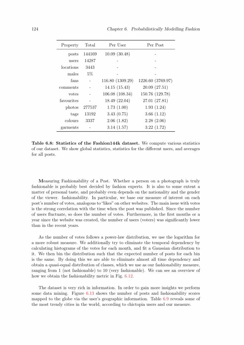
124 Chapter 6. Probabilistically Modelling Fashion
Property Total Per User Per Post
posts 144169 10.09 (30.48) -
users 14287 - -
locations 3443 - -
males 5% - -
fans - 116.80 (1309.29) 1226.60 (3769.97)
comments - 14.15 (15.43) 20.09 (27.51)
votes - 106.08 (108.34) 150.76 (129.78)
favourites - 18.49 (22.04) 27.01 (27.81)
photos 277537 1.73 (1.00) 1.93 (1.24)
tags 13192 3.43 (0.75) 3.66 (1.12)
colours 3337 2.06 (1.82) 2.28 (2.06)
garments - 3.14 (1.57) 3.22 (1.72)
Table 6.8: Statistics of the Fashion144k dataset. We compute various statisticsof our dataset. We show global statistics, statistics for the different users, and averagesfor all posts.
Measuring Fashionability of a Post. Whether a person on a photograph is trulyfashionable is probably best decided by fashion experts. It is also to some extent amatter of personal taste, and probably even depends on the nationality and the genderof the viewer. fashionability. In particular, we base our measure of interest on eachpost’s number of votes, analogous to “likes” on other websites. The main issue with votesis the strong correlation with the time when the post was published. Since the numberof users fluctuate, so does the number of votes. Furthermore, in the first months or ayear since the website was created, the number of users (voters) was significantly lowerthan in the recent years.
As the number of votes follows a power-law distribution, we use the logarithm fora more robust measure. We additionally try to eliminate the temporal dependency bycalculating histograms of the votes for each month, and fit a Gaussian distribution toit. We then bin the distribution such that the expected number of posts for each binis the same. By doing this we are able to eliminate almost all time dependency andobtain a quasi-equal distribution of classes, which we use as our fashionability measure,ranging from 1 (not fashionable) to 10 (very fashionable). We can see an overview ofhow we obtain the fashionability metric in Fig. 6.12.
The dataset is very rich in information. In order to gain more insights we performsome data mining. Figure 6.13 shows the number of posts and fashionability scoresmapped to the globe via the user’s geographic information. Table 6.9 reveals some ofthe most trendy cities in the world, according to chictopia users and our measure.

6.3. Modelling Fashionability 125
City Name Posts Fashionability
Manila 4269 6.627
Los Angeles 8275 6.265
Melbourne 1092 6.176
Montreal 1129 6.144
Paris 2118 6.070
Amsterdam 1111 6.059
Barcelona 1292 5.845
Toronto 1471 5.765
Bucharest 1385 5.667
New York 4984 5.514
London 3655 5.444
San Francisco 2880 5.392
Madrid 1747 5.371
Vancouver 1468 5.266
Jakarta 1156 4.398
Table 6.9: Mean fashionability of cities with at least 1000 posts. We computethe mean fashionability of all the posts from the different cities in the dataset. We thenshow the most fashionable cities with at least 1000 posts.
Feature Dim. Description
Fans 1 Number of user’s fans.
∆T 1 Time between post creation and download.
Comments 5 Sentiment analysis (Socher et al., 2013) of comments.
Location 266 Distance from location clusters (Simo-Serra et al., 2014b).
Personal 21 Face recognition attributes.
Style 20 Style of the photography (Karayev et al., 2014).
Scene 397 Output of scene classifier trained on (Xiao et al., 2010).
Tags 209 Bag-of-words with post tags.
Colours 604 Bag-of-words with colour tags.
Singles 121 Bag-of-words with split colour tags.
Garments 1352 Bag-of-words with garment tags.
Table 6.10: Overview of the different features used.

126 Chapter 6. Probabilistically Modelling Fashion
0 2 4 6 8 100
5000
10000
15000
20000
Binned Votes
0 1 2 3 4 5 6 7 80
2000
4000
6000
8000
Logarithm of Votes
0 200 400 600 800 10000
5000
10000
15000
20000
25000
30000
35000
Votes
4 2 0 2 40
2000
4000
6000
8000
10000
12000
14000
16000
Time Normalized Votes
Logarithm Non-linearBinning
TimeNormalization
Figure 6.12: Normalization of votes. We objectively model fashionability using thevotes. In order to remove the temporal component of the votes we perform a non-linearbinning on the logarithm of the votes for a specific month. We note that it is not a flatdistribution as we might have hoped. This is because we make an assumption that thevotes have a Gaussian distribution, which is not entirely true.
Pos
tD
ensi
ty
0.0
0.1
0.2
0.3
0.4
0.5
0.6
0.7
0.8
0.9
1.0
Fas
hio
nab
ility
0.0
0.1
0.2
0.3
0.4
0.5
0.6
0.7
0.8
0.9
1.0
Figure 6.13: Visualization of the density of posts and fashionability by coun-try. In the top row we show the logarithm of the number of posts per country as arepresentation of post density. In the bottom row we show the mean fashionability ofthe posts for all the countries.
Discovering Fashion from Weak Data
Our objective is not only to be able to predict fashionability of a given post, but wewant to create a model that can understand fashion at a higher level. For this purpose

6.3. Modelling Fashionability 127
Fans
Personal
Location
Scene
Colours
Singles
Garments
ΔTComments
Style
Tags
Figure 6.14: An overview of the CRF model and the features used by eachof the nodes.
we make use of a Conditional Random Field (CRF) to learn the different outfits, typesof people and settings. Settings can be interpreted as where the post is located, bothat a scenic and geographic level. Our potentials make use of deep networks over a widevariety of features exploiting Fashion144k images and meta-data to produce accuratepredictions of how fashionable a post is.
More formally, let u ∈ {1, · · · , NU} be a random variable capturing the type of user,o ∈ {1, · · · , NO} the type of outfit, and s ∈ {1, · · · , NS} the setting. Further, we denotef ∈ {1, · · · , 10} as the fashionability of a post x. We represent the energy of the CRF asa sum of energies encoding unaries for each variable as well as non-parametric pairwisepotentials which reflect the correlations between the different random variables. Wethus define
E(u, o, s, f) = Euser(u) + Eout(o) + Eset(s) + Efash(f)
+ Eufnp (u, f) + Eofnp(o, f) + Esfnp(s, f)
+ Euonp(u, o) + Esonp(s, o) + Eusnp(u, s) (6.16)
We refer the reader to Fig. 6.14 for an illustration of the graphical model. We nowdefine the potentials in more detail.
User: We compute user specific features encoding the logarithm of the number of fansthat the particular user has as well as the output of a pre-trained neural network-basedface detector enhanced to predict additional face-related attributes. In particular, weuse rekognition.com which computes attributes such as ethnicity, emotions, age, beauty,etc. We run this detector on all the images of each post and only keep the features forthe image with the highest score. We then compute our unary potentials as the outputof a small neural network with two hidden layers that takes as input the user’s highdimensional features and produces an 8D feature map φu(x). We refer the reader toFig. 6.15 for an illustration. Our user unary potentials are then defined as
Euser(u = i,x) = wTu,iφu(x)
with x all the information included in the post. Note that we share the features andlearn a different weight for each user latent state.

128 Chapter 6. Probabilistically Modelling Fashion
Fans
PersonalScene
Location
Singles
Colours
Garments
Comments
ΔT
Tags
Style
Softmax
Figure 6.15: Illustration of the type of deep network architecture used tolearn features. We can see that it consists of four network joined together by asoftmax layer. The output of the different networks φf , φo, φu, and φs are then usedas features for the CRF.
Outfit: We use a bag-of-words approach on the “garments” and “colours” meta-dataprovided in each post. Our dictionary is composed of all words that appear at least 50times in the training set. This results in 1352 and 604 words respectively and thus ourrepresentation is very sparse. Additionally we split the colour from the garment in the“colours” feature, e.g., red-dress becomes red and dress, and also perform bag-of-wordson this new feature. We then compute our unary potentials as the output of a smallneural network with two hidden layers that takes as input the outfit high dimensionalfeatures and produces an 8D feature map φo(x). We refer the reader to Fig. 6.15 foran illustration. Our outfit unary potentials are then defined as
Eout(o = i,x) = wTo,iφo(x)
with x all the information included in the post. Note that as with the users we sharethe features and learn a different weight for each outfit latent state.
Setting: We try to capture the setting of each post by using both a pre-trained sceneclassifier and the user-provided location. For the scene classifier we have trained amulti-layer perceptron with a single 1024 unit hidden layer and softmax layer on theSUN Dataset (Xiao et al., 2010). We randomly use 70% of the 130,519 images as thetraining set, 10% as the validation set and 20% as the test set. We use the Caffepre-trained network (Jia, 2013) to obtain features for each image which we then use tolearn to identify each of the 397 classes in the dataset, corresponding to scenes such as“art_studio”, “vineyard” or “ski_slope”. The output of the 397D softmax layer is usedas a feature along with the location. As the location is written in plain text, we firstlook up the latitude and longitude. We project all these values on the unit sphere andadd some small Gaussian noise to account for the fact that many users will write moregeneric locations such as “Los Angeles" instead of the real address. We then performunsupervised clustering using geodesic distances (Simo-Serra et al., 2014b) and use thegeodesic distance from each cluster center as a feature. We finally compute our unarypotentials as the output of a small neural network with two hidden layers that takesas input the settings high dimensional features and produce an 8D feature map φs(x).

6.3. Modelling Fashionability 129
Our outfit unary potentials are then defined as
Eset(s = i,x) = wTs,iφs(x)
with x all the information included in the post. Note that as with the users and outfitswe share the features and learn a different weight for each settings latent state.
Fashion: We use the time between the creation of the post and when the post wascrawled as a feature, as well as bag-of-words on the “tags”. To incorporate the reviews,we parse the comments with the sentiment-analysis model of (Socher et al., 2013).This model attempts to predict how positive a review is on a 1-5 scale (1 is extremelynegative, 5 is extremely positive). We used a pre-trained model that was trained on therotten tomatoes dataset. We run the model on all the comments and sum the scoresfor each post. We also extract features using the style classifier proposed in (Karayevet al., 2014) that is pre-trained on the Flickr80k dataset to detect 20 different imagestyles such as “Noir”, “Sunny”, “Macro” or “Minimal”. This captures the fact that agood photography style is correlated with the fashionability score. We then computeour unary potentials as the output of a small neural network with two hidden layersthat takes as input the settings high dimensional features and produce an 8D featuremap φf (x). Our outfit unary potentials are then defined as
Efash(f = i,x) = wTf,iφf (x)
Once more, we shared the features and learn separate weights for each fashionabilityscore.
Correlations: We use a non-parametric function for each pairwise and let the CRFlearn the correlations. Thus
Eufnp (u = i, f = j) = wufi,j
Similarly for the other pairwise potentials.
Learning and Inference
We learn our model using a two step approach: we first jointly train the deep networksthat are used for feature extraction to predict fashionability as shown in Fig 6.15, andestimate the initial latent states using clustering. We then learn the CRF model (2430weights) using the primal-dual method of (Hazan and Urtasun, 2010). In particular,we use the implementation of (Schwing et al., 2012). As task loss we use the L1 normfor fashionability, and encourage the latent states to match the initial clustering. Weperform inference using message passing (Schwing et al., 2011).
Experimental Evaluation
We perform a detailed quantitative evaluation on the 10-class fashionability predictiontask. Furthermore, we provide a qualitative evaluation on other high level tasks suchas visualizing changes in trends and outfit recommendations.

130 Chapter 6. Probabilistically Modelling Fashion
Attribute Corr.
Economy class -0.137
Income class -0.111
log(GDP) 0.258
log(Population) 0.231
Attribute Corr.
age -0.025
beauty 0.066
eye_closed 0.022
gender -0.037
smile -0.023
asian 0.024
calm 0.023
happy -0.024
sad 0.023
Table 6.11: Effect of various attributes on the fashionability. Economy andIncome class refer to a 1-7 scale in which 1 corresponds to most developed or richcountry while 7 refers to least developed or poor country. For the face recognitionfeatures we only show those with absolute values above 0.02. In all cases we show thePearson Coefficients.
Mea
nB
eauty
0.0
0.1
0.2
0.3
0.4
0.5
0.6
0.7
0.8
0.9
1.0
Dom
inan
tE
thnic
ity
American
Indian
Asian
Black
Indian
White
Figure 6.16: Visualization of mean beauty and dominant ethnicity by coun-try. We average the beauty and ethnicity scores of all posts and show results for allthe countries.

6.3. Modelling Fashionability 131
Model Acc. Pre. Rec. IOU L1
CRF 29.27 30.42 28.69 17.36 1.46
Deep Net 30.42 31.11 30.26 18.41 1.45
Log. Reg. 23.92 22.54 22.99 12.55 1.91
Baseline 16.28 - 10.00 1.63 2.32
Random 9.69 9.69 9.69 4.99 3.17
Table 6.12: Fashionability prediction results.We show results for classification forrandom, a baseline that predicts only the dominant class, a standard logistic regressionon our features, the deep network used to obtain features for the CRF and the finalCRF model. We show accuracy, precision, recall, intersection over union (IOU), and L1
norm as different metrics for performance.
Correlations
We first analyze the correlation between fashionability and various features in our model.We consider the effect of the country on fashionability: in particular, we look the effectof economy, income class, Gross Domestic Product (GDP) and population. Resultsare in Table 6.11-left. A strong relationship is clear: poorer countries score lower infashionability than the richer, sadly a not very surprising result.
We also show face-related correlations in Table 6.11-right. Interestingly, but notsurprising, younger and more beautiful users are considered more fashionable. Addi-tionally, we show the mean estimated beauty and dominant inferred ethnicity on theworld map in Fig. 6.16. Brazil dominates the Americas in beauty, France dominatesSpain, and Turkey dominates in Europe. In Asia, Kazakhstan scores highest, followedby China. There are also some high peaks which may be due to a very low number ofposts in a country. The ethnicity classifier also seems to work pretty well, as generallythe estimation matches the ethnicity of the country.
Predicting Fashionability
We use 60% of the dataset as a train set, 10% as a validation, and 30% as test, andevaluate our model for the fashionability prediction task. Results of various modelinstantiations are reported in Table 6.12. While the deep net obtains slightly betterresults than our CRF, the model we propose is very useful as it simultaneously identifiesthe type of user, setting and outfit of each post. Additionally, as we show later, theCRF model allows performing much more flexible tasks such as outfit recommendationor visualization of trends. Since the classification metrics such as accuracy, precision,recall, and intersection over union (IOU) do not capture the relationship between thedifferent fashionability levels, we also report the L1 norm between the ground truth andthe predicted label. In this case both the CRF and the deep net obtain virtually thesame performance.
Furthermore, we show qualitative examples of true positives, false positives, truenegatives and false positives in Fig. 6.17. Note that while we are only visualizingimages, there is a lot of meta-data associated to each image.

132 Chapter 6. Probabilistically Modelling Fashion
Tru
ePos
itiv
esFal
sePos
itiv
es
Figure 6.17: True and false positive fashionability prediction examples. Weshow some examples of the classification task obtained with our CRF model.
Feature Single feature Leave one out
Baseline 16.3 23.9
Comments 19.7 21.6
Tags 17.4 23.7
∆T 17.2 23.4
Style 16.3 23.4
Location 16.9 23.3
Scene 16.1 23.3
Fans 18.9 23.2
Personal 16.3 23.1
Colours 15.9 23.0
Singles 17.2 22.8
Garments 16.2 22.7
Table 6.13: Evaluation of features for predicting fashionability. We evaluatethe different features for the fashionability prediction task using logistic regression. Weshow two cases: performance of individual features, and performance with all but onefeature, which we call leave one out.

6.3. Modelling Fashionability 133
Dom
inan
tSet
tings
Clu
ster
MosqueSuburbiaClaustrophobicInterior SmallOrchardSportsOutdoors RedVolcanoBeachInterior WideFarmSkiSpringsBaseballCoffeeSnowy MountainsVinyardLockersMarketPlayground
Dom
inan
tO
utfi
tC
lust
er
Black Heavy
Pastel Shirts/Skirts
Shoes and Blue Dress
Pink/Black Misc.
Heels
Black Casual
Pink Outfit
Shirts and Jeans
Blue with Scarf
Black with Bag/Glasses
Pastel Dress
Black/Gray Tights/Sweater
Pink/Blue Shoes/Dress/Shorts
Bags/Dresses
Navy and Bags
Brown/Blue Jacket
White/Black Blouse/Heels
Black Boots/Tights
Formal Blue/Brown
Black/Blue Going out
Figure 6.18: Visualization of the dominant latent clusters. We show results forthe settings and outfit nodes in our CRF by country.
In order to analyze the individual contribution of each of the features, we showtheir individual prediction power as well as how much performance is lost when afeature is removed. The individual performances of the various features are shown inthe second column of Table 6.13. We can see that in general the performance is verylow. Several features even perform under the baseline (Personal, Scene, and Colours).The strongest features are Comments and Fans, which, however, are still not a verystrong indicator of fashionability as one would expect. In the leave one out case shownin the third column, removing any feature causes a drop in performance. This meansthat some features are not strong individually, but carry complementary information toother features and thus still contribute to the whole. In this case we see that the mostimportant feature is once again Comments, likely caused by the fact that most usersthat comment positively on a post also give it a vote.
Identifying Latent States
In order to help interpreting the results we manually attempt to give semantic meaningto the different latent states discovered by our model. While some states are harder toassign a meaning due to the large amount of data variation, other states like, e.g., thesettings states corresponding to “Ski” and “Coffee” have a clear semantic meaning. Avisualization of the location of some of the latent states can be seen in Fig. 6.18.
By visualizing the pairwise weights between the fashionability node and the differentnodes we can also identify the “trendiness” of different states (Fig. 6.19). For example,the settings state 1 corresponding to “Mosque” is clearly not fashionable while the state2 and 3 corresponding to “Suburbia” and “Claustrophobic”, respectively, have positivegradients indicating they are fashionable settings.

134 Chapter 6. Probabilistically Modelling Fashion
Setting Class
Fashio
nabili
ty
1 2 3 4 5 6 7 8 9 10 11 12 13 14 15 16 17 18 19 20
1
2
3
4
5
6
7
8
9
10
−15
−10
−5
0
5
10
User Class
Fashio
nabili
ty
1 2 3 4 5 6 7 8 9 10 11 12 13 14 15 16 17 18 19 20
1
2
3
4
5
6
7
8
9
10
−2
−1
0
1
2
Outfit Class
Fashio
nabili
ty
1 2 3 4 5 6 7 8 9 10 11 12 13 14 15 16 17 18 19 20
1
2
3
4
5
6
7
8
9
10
−6
−4
−2
0
2
4
Figure 6.19: Visualizing pairwise potentials between nodes in the CRF. Bylooking at the pairwise between fashionability node and different states of other variableswe are able to distinguish between fashionable and non-fashionable outfits and settings.

6.3. Modelling Fashionability 135
Current Outfit:
Pink/Black Misc. (5)
Recommendations:
Pastel Dress (8)
Black/Blue Going out (8)
Black Casual (8)
Current Outfit:
Pink Outfit (3)
Recommendations:
Heels (8)
Pastel Shirts/Skirts (8)
Black/Gray Tights/Sweater (5)
Current Outfit:
Pink/Blue Shoes/Dress Shorts (3)
Recommendations:
Black/Gray Tights/Sweater (5)
Black Casual (5)
Black Boots/Tights (5)
Current Outfit:
Blue with Scarf (3)
Recommendations:
Heels (8)
Pastel Shirts/Skirts (8)
Black Casual (8)
Current Outfit:
Pink/Blue Shoes/Dress Shorts (3)
Recommendations:
Black Casual (7)
Black Heavy (3)
Navy and Bags (3)
Current Outfit:
Formal Blue/Brown (5)
Recommendations:
Pastel Shirts/Skirts (9)
Black/Blue Going out (8)
Black Boots/Tights (8)
Figure 6.20: Examples of recommendations provided for our model. In paren-thesis we see the fashionability of the user as predicted by our model.
Black Heavy
Pastel Shirts/Skirts
Shoes and Blue Dress
Pink/Black Misc.
Heels
Black Casual
Pink Outfit
Shirts and Jeans
Blue with Scarf
Black with Bag/Glasses
Pastel Dress
Black/Gray Tights/Sweater
Pink/Blue Shoes/Dress/Shorts
Bags/Dresses
Navy and Bags
Brown/Blue Jacket
White/Black Blouse/Heels
Black Boots/Tights
Formal Blue/Brown
Black/Blue Going out
0.00
0.05
0.10
0.15
0.20
0.25
0.30
0.35
Trimester
Los Angeles
201612840.0
0.1
0.2
0.3
0.4
0.5
0.6
Trimester
Manila
20161284
Figure 6.21: Visualization of the temporal evolution of the different trends inManila and Los Angeles. The less significant clusters have been manually removedto decrease clutter.
Outfit Recommendation
An exciting property of our model is that it can be used for outfit recommendation.In this case, we take a post as an input and estimate the outfit that maximizes thefashionability while keeping the other variables fixed. In other words, we are predictingwhat the user should be wearing in order to maximize her/his look instead of theircurrent outfit. We show some examples in Fig. 6.20. This is just one example of theflexibility of our model. Other tasks such what is the least fitting outfit, what is thebest place to go to with the current outfit, or what types of users this outfit fits themost, can also be done with the same model.

136 Chapter 6. Probabilistically Modelling Fashion
Estimation Fashion Trends
By incorporating temporal information we can try to visualize the changes in trendsfor a given location. In particular we look at the trendiest cites in the dataset, that isManila and Los Angeles, as per Table 6.9. We visualize these results in Fig. 6.21. ForManila, one can see that while until the 8th trimester, outfits like “Pastel Skirts/Shirts”and “Black with Bag/Glasses” are popular, after the 12th trimester there is a boom of“Heels” and “Pastel Dress”. Los Angeles follows a roughly similar trend. For LA however,before the 8th trimester, “Brown/Blue Jacket” and “Pink/Black Misc” are popular,while afterwards “Black Casual” is also fairly popular. We’d like to note that in the 8thtrimester there appears to have been an issue with the chictopia website, causing veryfew posts to be published, and as a consequence, results in unstable outfit predictions.
6.4 Summary
In this chapter we have dealt with understanding images in the challenging context offashion. This has only recently become the focus of research and is proving to requiremany innovations in order to have competitive results. It is an exciting topic that canprove to be invaluable to users in an era in which one’s personal image is critical to besuccessful in society: from applying to universities to finding a job, and even to succeedin one’s love life.
First we have tackled the challenging problem of clothing parsing in fashion images.We have shown that our approach is able to obtain a significant improvement overthe state-of-the-art in the challenging Fashionista dataset by exploiting appearance,figure/ground segmentation, shape and location priors for each garment as well as sim-ilarity between segments and symmetries between different human body parts. Despitethese promising results, we believe much can still be done to improve. For example, oneof the most occurring mistakes are missing glasses or other small garments. We believea multi-resolution approach is needed to handle the diversity of garment classes.
We have also presented a novel task of predicting fashionability of users photographs.In order to evaluate this task we have collected a large-scale dataset by crawling thelargest fashion-oriented social website. Our proposed Conditional Random Fields modelis able to reason about settings, users and their fashionability. We are able to predictthe visual aesthetics related to fashion, which can also be used to analyze fashiontrends in the world or individual cities, and potentially different age groups and outfitstyles. Furthermore our model can also be used for outfit recommendation. This is animportant first step to building more complex and powerful models that will be ableto understand fashion, trends, and users a whole in order to improve the experience ofusers in the modern day society. We will make the dataset and code public in hopesthat this will inspire other researchers to tackle this challenging task.
It is important to note that to obtain our competitive results in these challengingtasks, many of the techniques and approaches developed in other chapter of this thesishave played a fundamental role. In order to perform high level tasks such as predictingfashionability it is essential to have a good grasp on mid and low level cues. It is nolonger sufficient to focus on a very niche problem with a narrow understanding of one’sfield.

Chapter 7
Conclusions
In this thesis we have analyzed the problem of understanding human-centric images atvarious levels. Our work is a push towards more ambitious goals such as estimatingfashionability and proposing better outfits which we presented in Chapter 6. In orderto be able to tackle these higher level tasks, we have presented a swath of techniquesfrom low level image features to full 3D pose estimation algorithms. We finally showedthe importance of using strong low and mid level cues in high level tasks.
To recapitulate the contributions:
1. We have proposed and evaluated two different approaches for local feature de-scription. On one hand, we have used heat diffusion to robustly describe imagepatches undergoing deformation and illumination changes. On the other hand,we have shown that it is not only possible to learn descriptors using convolutionalnetworks, but also extremely beneficial when done with high levels of mining de-noted “fracking”.
2. For 3D human pose estimation and other problems we have investigated severalgenerative models. In particular, we presented two novel models for representing3D human pose. One is based on a Directed Acyclic Graph with a discrete repre-sentation of the poses, and is used to learn a mapping between a latent space andthe pose space. The other models the pose as data on a Riemannian manifoldusing a Gaussian mixture with local approximations.
3. We have also presented two frameworks for 3D human pose estimation from singlemonocular images. We show how it is possible to use noisy 2D observationsto obtain more reliable 3D pose estimations. Additionally, we demonstrate thebenefits of integrating the 2D and 3D pose estimation into a single end-to-endsystem that performs both tasks simultaneously.
4. Finally, we show more higher level applications in the challenging context of fash-ion. In particular, we show results with a Conditional Random Fields model us-ing very strong mid level cues for the complex task of semantic segmentation ofclothing. We also propose the novel high level task of predicting fashionabilityfrom images. We show it is possible to design models that are able to interpretthe image and provide recommendations on how to improve one’s fashionableness.
137

138 Chapter 7. Conclusions
All these works share the same context, that is, they are designed for usage inhuman-centric images. While the lower level approaches such as descriptors and gener-ative models do also generalize to many other problems, the 3D human pose estimationapproaches and the fashion understanding developments are specific to human-centricimages.
Additionally, we would like to point out we have made most of the code and datasetsof this thesis publicly available1. We believe this is important for the reproducibility ofour results and for the benefit of the community in general. We acknowledge that thereare still parts of this thesis not made publicly available, however, we have the intentionof releasing more in the near future.
7.1 Future Work
We have set the basis for many different tools that we have not yet fully exploited inthis thesis. The most direct line of work is to attempt to take more advantage of ourlow and mid level cues in other tasks. In particular our descriptors have not been testedin full applications yet, although they have been thoroughly evaluated on real images.
For more tangible directions of work, we can refer to our deep learning approachfor feature point descriptors. In particular, while we were able to obtain great improve-ments, there are still many open questions. For example, is it possible to learn robust-ness to different types of properties, such as rotation or scale, independently? Whatexactly is the effect of the training data on a pre-learned network? Is it possible toexploit other datasets in order to obtain better generalizations? It is also not clearwhether the best performing network’s hyperparameters are optimal. This requiresa much more high level large-scale analysis and in particular the creation of a morecomplete large dataset for feature point matching.
Our generative model based on clustering on Riemannian manifolds also has showngreat promise, but has not been used in a real 3D pose estimation framework. As thestrength of this model holds on the fact it can quickly estimate distributions for missinglimbs, if it were feasible to integrate it with an occlusion estimator, it would be possibleto handle occlusions in an elegant manner. Furthermore, as we show in (Simo-Serraet al., 2015c), it is possible to use the same framework for tracking. Therefore anotherlogical extension of the work presented in this thesis would be to tackle the problem of3D human pose tracking. This would require extending the Bayesian formulation of oursimultaneous 2D and 3D human pose estimation to integrate the temporal component.
Finally, we have only started to explore the possibilities in the world of fashion. Wehave presented a novel large dataset called Fashion144k for the prediction of fashion-ability, but have only started approaching this challenging problem. As shown by ourpreliminary results, this is a very complex problem which requires development of muchstronger features and cues, such as our clothing segmentation algorithm, in order to beable to perform reliable predictions. Additionally, due to the large scale of the dataset,it is imperative for these feature extraction algorithms to be fast and scale well to thesize of the dataset. For this purpose, we think it is fundamental to try to develop newapproaches as well as explore the existing literature to see what cues we can exploit tobuild models that can truly understand fashion.
1http://www.iri.upc.edu/people/esimo/
7.2. Trends in Computer Vision and Machine Learning 139
7.2 Trends in Computer Vision and Machine Learning
In the elaboration of this thesis, we have exploited many existing tools from the fieldsof computer vision and machine learning. As both these fields are moving extremelyfast, we would like to briefly mention some major changes we have experienced duringthe course of this thesis and give insights as to which direction we believe it is heading.
Probably the strongest change we have been able to experience has been the ir-ruption of deep learning in computer vision. At the beginning of the thesis (2011),these tools were not widely available nor very relevant, however, since the publicationof (Krizhevsky et al., 2012) we have seen a large influx of incredible results that havebeen overturning most well established techniques (Girshick et al., 2014; Simonyan andZisserman, 2014). While the pure quantitative results of these approaches have beenunbeatable in most tasks, a number of concerned voices have appeared questioningwhether or not we fully understand them. This has led to the current trend of not onlyobtaining great results with these systems, but also understanding why we are able toobtain these great results (Zeiler and Fergus, 2014; Chatfield et al., 2014).
Competing with alternative approaches against deep learning in many problemssuch as classification seems like a lost cause. Not only because it seems like no otheralgorithms can compete with them on certain problems, but additionally the resourcessome of the next generation of networks require to train are out of the reach of allexcept the largest research laboratories. The unrelenting increase of available data andthe infrastructure needed to process them are a concern for the competitiveness of smallresearch centers. However, despite the enormous results on classifications, and morerecently detection, problems, we believe there are still holes that can’t be filled withpure deep learning approaches. For example structured prediction problems in whichthe output is subject to a set of constraints are very complicated to model with neuralnetworks.
While results in problems with more tradition have been greatly affected by the deeplearning tsunami, we have also seen an emergence of very interesting new problems incomputer vision. Related to this thesis we have seen the first dataset for segmentation infashion images in 2012 (Yamaguchi et al., 2012). In tune with this, we proposed our owndataset for predicting fashionionability and presented the novel task of giving fashionadvice. On a similar line of research it is also worth to mention the work of (Pirsiavashet al., 2014), which attempts to assess different actions performed by a user, such aspool diving or figure skating, and give advice on how to improve the performance of theaction. Another interesting and recent line of research seeks to find out what makesphotographs of faces memorable and attempts to modify them to become even more so(Khosla et al., 2013). These are all very high level tasks that were unthinkable just afew years back. We believe we are at a point of inflection and things that were sciencefiction just a decade back will start to become more and more commonplace.
Another heavily questioned aspect is currently the publication model in computervision and machine learning. There is already an antecedent of a major change in themachine learning literature when forty members resigned from the Editorial Board ofthe Machine Learning Journal (MLJ), and moved to support the newly created Journalof Machine Learning Research (JMLR) (Jordan, 2001). This was a move away fromrestricted access pay-per-view to a free-access model, which we personally believe hasgreatly benefited the community. Along the same lines, during the Computer Visionand Pattern Recognition (CVPR) 2013 conference in Portland, Oregon, moving to an

140 Chapter 7. Conclusions
open access model was also decided by voting (PAMI-TC, 2013). This is the unavoidableconsequence of the distribution abilities of the internet and the widespread practice ofresearchers hosting their papers on their website to encourage diffusion.
In 2013 we additionally saw the birth of a completely new publication model.The new deep learning oriented International Conference on Learning Representations(ICLR) had its first edition. Instead of using the well established double-blind reviewprocess with a rebuttal period, they opted for single blind reviewing process, which wascommon in machine learning over a decade ago. This may seem like a step backwards,however, this is the consequence of moving to an open review model 2. In this confer-ence papers are put online during submission time and the entire reviewing process ismade transparent, i.e., reviews and responses are public and shown in realtime. Addi-tionally, editing of the paper after the initial submission is actively encouraged. Thisdrastically changes the publication model and is once again the inevitable result of anew widespread practice: publishing preliminary work on the arXiv website 3 whensubmitting to a top-tier conference such as CVPR. While it is not clear if this newmodel is more fair than double-blind reviewing, it provides an interesting alternativefor a time when it is hard to enforce the anonymousness of the submitting authors.
Finally, very recently we have seen the results of a most interesting experiment. Thedenoted “NIPS Experiment” (Price, 2014) consisted of forming two independent programcommittees and assigning a random 10% of submitted papers to both committees. Theambitious objective of this feat was to quantify the amount of randomness in acceptanceof papers. Anyone who has submitted to a research conference is familiar with thisrandomness. A poll of submitters indicated that most agreed that the divergence wouldbe found to be around 30%. During the conference in December 2014 the results werepublished and it was found that an astounding 57% of accepted papers would havebeen rejected by the other reviewing team. The implications of this result are not yetunderstood.
As we can see, not only has there been a landslide in the techniques used for com-puter vision with the irruption of deep learning, there have also been many changes asthe current publishing model is being questioned. We believe that there are still moreimportant changes to come in the short term, however, they seem to be going in theright direction and will be beneficial to the future of our research.
2http://www.iclr.cc/doku.php?id=pubmodel3http://arxiv.org/

Bibliography
A. Yao, J. Gall, L. V. G. and Urtasun, R. (2011). Learning probabilistic non-linear latentvariable models for tracking complex activities. In Neural Information ProcessingSystems. 65
Achanta, R., Shaji, A., Smith, K., Lucchi, A., Fua, P., and Susstrunk, S. (2012). Slicsuperpixels compared to state-of-the-art superpixel methods. IEEE TransactionsPattern Analylis and Machine Intelligence, 34(11):2274–2282. 9
Agarwal, A. and Triggs, B. (2006). Recovering 3d human pose from monocular images.IEEE Transactions Pattern Analylis and Machine Intelligence, 28(1):44–58. 85
Andriluka, M., Roth, S., and Schiele, B. (2009). Pictorial Structures Revisited: PeopleDetection and Articulated Pose Estimation. In IEEE Conference on Computer Visionand Pattern Recognition. 83, 86, 87, 96, 97, 98
Andriluka, M., Roth, S., and Schiele, B. (2010). Monocular 3D Pose Estimation andTracking by Detection. In IEEE Conference on Computer Vision and Pattern Recog-nition. 65, 66, 83, 85, 87, 92, 93, 94, 100, 101, 102
Andriluka, M., Roth, S., and Schiele, B. (2012). Discriminative Appearance Models forPictorial Structures. International Journal of Computer Vision, 99(3). 69, 83, 97
Anguelov, D., Srinivasan, P., Koller, D., Thrun, S., Rodgers, J., and Davis, J. (2005).Scape: shape completion and animation of people. ACM Transactions on Graphics,24(3):408–416. 65
Balan, A. O., Sigal, L., Black, M. J., Davis, J. E., and Haussecker, H. W. (2007).Detailed Human Shape and Pose from Images. In IEEE Conference on ComputerVision and Pattern Recognition. 84, 85
Bay, H., Tuytelaars, T., and Gool, L. V. (2006). SURF: Speeded up robust features. InEuropean Conference on Computer Vision, pages 404–417. 23, 25, 49, 50
Belongie, S., Malik, J., and Puzicha, J. (2002). Shape matching and object recognitionusing shape contexts. IEEE Transactions Pattern Analylis and Machine Intelligence,24(4):509–522. 25
141

142 Bibliography
Berg, A., Berg, T., and Malik, J. (2005). Shape matching and object recognition usinglow distortion correspondences. In IEEE Conference on Computer Vision and PatternRecognition, volume 1, pages 26–33. 25
Bo, L. and Sminchisescu, C. (2010). Twin Gaussian Processes for Structured Prediction.International Journal of Computer Vision, 87:28–52. 83, 93, 94, 101, 102
Boothby, W. M. (2003). An Introduction to Differentiable Manifolds and RiemannianGeometry. Revised 2nd Ed. Academic, New York. 74
Bossard, L., Dantone, M., Leistner, C., Wengert, C., Quack, T., and Gool, L. V. (2012).Apparel classifcation with style. In Asian Conference on Computer Vision. 106, 108
Bourdev, L., Maji, S., and Malik, J. (2011). Describing people: A poselet-based ap-proach to attribute classification. In International Conference on Computer Vision.106, 108
Bourdev, L. and Malik, J. (2009). Poselets: Body part detectors trained using 3d humanpose annotations. In International Conference on Computer Vision. 108
Boykov, Y., Veksler, O., and Zabih, R. (2001). Fast approximate energy minimiza-tion via graph cuts. IEEE Transactions Pattern Analylis and Machine Intelligence,23(11):1222–1239. 14
Bromley, J., Guyon, I., Lecun, Y., Säckinger, E., and Shah, R. (1994). Signatureverification using a "siamese" time delay neural network. In Neural InformationProcessing Systems. 50
Bronstein, A., Bronstein, M., Bruckstein, A., and Kimmel, R. (2007). Analysis of two-dimensional non-rigid shapes. International Journal of Computer Vision, 78(1):67–88.25
Bronstein, M. and Kokkinos, I. (2010). Scale-invariant heat kernel signatures for non-rigid shape recognition. In IEEE Conference on Computer Vision and Pattern Recog-nition, pages 1704–1711. 24, 29
Brown, M., Hua, G., and Winder, S. (2011). Discriminative learning of local image de-scriptors. IEEE Transactions Pattern Analylis and Machine Intelligence, 33(1):43–57.49, 50, 51, 53
Brox, T., Bourdev, L., Maji, S., and Malik, J. (2011). Object segmentation by alignmentof poselet activations to image contours. In IEEE Conference on Computer Visionand Pattern Recognition. 108
Brubaker, M. A., Salzmann, M., and Urtasun, R. (2012). A Family of MCMC Methodson Implicitly Defined Manifolds. Journal of Machine Learning Research - ProceedingsTrack, 22:161–172. 65, 73
Burenius, M., Sullivan, J., and Carlsson, S. (2013). 3d pictorial structures for multipleview articulated pose estimation. In IEEE Conference on Computer Vision andPattern Recognition. 83

Bibliography 143
C. Strecha, A. Bronstein, M. B. and Fua, P. (2012). LDAHash: Improved matching withsmaller descriptors. IEEE Transactions Pattern Analylis and Machine Intelligence,34(1). 40, 50, 60
Cai, H., Mikolajczyk, K., and Matas, J. (2011). Learning linear discriminant projec-tions for dimensionality reduction of image descriptors. IEEE Transactions PatternAnalylis and Machine Intelligence, 33(2):338–352. 40
Calonder, M., Lepetit, V., Ozuysa, M., Trzcinski, T., Strecha, C., and Fua, P. (2012).BRIEF: Computing a local binary descriptor very fast. IEEE Transactions PatternAnalylis and Machine Intelligence, 34(7):1281–1298. 25
Carreira, J., Caseiroa, R., Batista, J., and Sminchisescu, C. (2012). Semantic segmen-tation with second-order pooling. In European Conference on Computer Vision. 12,110, 111, 112, 117, 118, 120
Carreira, J. and Sminchisescu, C. (2012). CPMC: Automatic Object SegmentationUsing Constrained Parametric Min-Cuts. IEEE Transactions Pattern Analylis andMachine Intelligence, 34(7):1312–1328. 11, 110
Chang, C.-C. and Lin, C.-J. (2011). LIBSVM: A library for support vector machines.ACM Transactions on Intelligent Systems and Technology, 2:27:1–27:27. 16
Chatfield, K., Simonyan, K., Vedaldi, A., and Zisserman, A. (2014). Return of the devilin the details: Delving deep into convolutional nets. CoRR, abs/1405.3531. 139
Chavel, I. (1984). Eigenvalues in Riemannian Geometry. London Academic Press. 28
Chen, H., Gallagher, A., and Girod, B. (2012). Describing clothing by semantic at-tributes. In European Conference on Computer Vision. 106, 108, 123
Chen, H., Xu, Z. J., Liu, Z. Q., and Zhu, S. C. (2006). Composite templates forcloth modeling and sketching. In IEEE Conference on Computer Vision and PatternRecognition. 108, 122
Cheng, H., Liu, Z., Zheng, N., and Yang, J. (2008). A deformable local image descriptor.In IEEE Conference on Computer Vision and Pattern Recognition. 23, 25
Cho, M., Lee, J., and Lee, K. (2009). Feature correspondence and deformable objectmatching via agglomerative correspondence clustering. In International Conferenceon Computer Vision, pages 1280–1287. 23, 25
Collobert, R., Kavukcuoglu, K., and Farabet, C. (2011). Torch7: A matlab-like envi-ronment for machine learning. In BigLearn, NIPS Workshop. 52
Culurciello, E., Jin, J., Dundar, A., and Bates, J. (2013). An analysis of the connectionsbetween layers of deep neural networks. CoRR, abs/1306.0152. 52
Dalal, N. and Triggs, B. (2005). Histograms of oriented gradients for human detection.In IEEE Conference on Computer Vision and Pattern Recognition. 9, 10, 83
Daubney, B. and Xie, X. (2011). Tracking 3D Human Pose with Large Root NodeUncertainty. In IEEE Conference on Computer Vision and Pattern Recognition. 65,83, 87, 93, 94, 101, 102

144 Bibliography
Davis, B. C., Bullitt, E., Fletcher, P. T., and Joshi, S. (2007). Population ShapeRegression from Random Design Data. In International Conference on ComputerVision. 65
Davis, J. and Goadrich, M. (2006). The relationship between PR and ROC curves. InInternational Conference in Machine Learning. 54
de Goes, F., Goldenstein, S., and Velho, L. (2008). A hierarchical segmentation ofarticulated bodies. In Proceedings of the Symposium on Geometry Processing, pages1349–1356. 26
Dedieu, J.-P. and Nowicki, D. (2005). Symplectic methods for the approximation of theexponential map and the newton iteration on riemannian submanifolds. Journal ofComplexity, 21(4):487 – 501. 74
Deng, J., Dong, W., Socher, R., jia Li, L., Li, K., and Fei-fei, L. (2009). Imagenet:A large-scale hierarchical image database. In IEEE Conference on Computer Visionand Pattern Recognition. 116
Dhar, S., Ordonez, V., and Berg, T. (2011). High level describable attributes for pre-dicting aesthetics and interestingness. In IEEE Conference on Computer Vision andPattern Recognition. 123
Donahue, J., Jia, Y., Vinyals, O., Hoffman, J., Zhang, N., Tzeng, E., and Darrell, T.(2013). Decaf: A deep convolutional activation feature for generic visual recognition.CoRR, abs/1310.1531. 13
Dong, J., Chen, Q., Xia, W., Huang, Z., and Yan, S. (2013). A deformable mixtureparsing model with parselets. In International Conference on Computer Vision. 108
Everingham, M., Van Gool, L., Williams, C. K. I., Winn, J., and Zisserman, A. (2010).The pascal visual object classes (voc) challenge. International Journal of ComputerVision, 88(2):303–338. 116
Fan, B., Wu, F., and Hu, Z. (2012). Rotationally invariant descriptors using inten-sity order pooling. IEEE Transactions Pattern Analylis and Machine Intelligence,34(10):2031–2045. 26
Fan, R.-E., Chang, K.-W., Hsieh, C.-J., Wang, X.-R., and Lin, C.-J. (2008). LIBLIN-EAR: A library for large linear classification. Journal of Machine Learning Research,9:1871–1874. 15
Farhadi, A., Endres, I., Hoiem, D., and Forsyth, D. (2009). Describing objects by theirattributes. In IEEE Conference on Computer Vision and Pattern Recognition. 13
Felzenszwalb, P., McAllester, D., and Ramanan, D. (2008). A Discriminatively Trained,Multiscale, Deformable Part Model. In IEEE Conference on Computer Vision andPattern Recognition. 1, 69, 86, 87
Felzenszwalb, P. F., Girshick, R. B., McAllester, D., and Ramanan, D. (2010). ObjectDetection with Discriminatively Trained Part Based Models. IEEE TransactionsPattern Analylis and Machine Intelligence, 32(9):1627–1645. 50, 69

Bibliography 145
Felzenszwalb, P. F. and Huttenlocher, D. P. (2005). Pictorial Structures for ObjectRecognition. International Journal of Computer Vision, 61:55–79. 3, 63, 83, 86
Fidler, S., Sharma, A., and Urtasun, R. (2013). A sentence is worth a thousand pixels.In IEEE Conference on Computer Vision and Pattern Recognition. 108
Figueiredo, M. and Jain, A. (2002). Unsupervised Learning of Finite Mixture Models.IEEE Transactions Pattern Analylis and Machine Intelligence, 24(3):381–396. 73, 76,77
Fletcher, P., Lu, C., Pizer, S., and Joshi, S. (2004). Principal Geodesic Analysis forthe Study of Nonlinear Statistics of Shape. IEEE Transactions on Medical Imaging,23(8):995–1005. 65, 66, 73
Forbes Magazine (2013). US Online Retail Sales To Reach $370B By 2017; e191B inEurope. http://www.forbes.com. [Online; accessed 14-March-2013]. 106
Gallagher, A. C. and Chen, T. (2008). Clothing cosegmentation for recognizing people.In IEEE Conference on Computer Vision and Pattern Recognition. 106, 108
Geiger, A., Lenz, P., Stiller, C., and Urtasun, R. (2013). Vision meets robotics: Thekitti dataset. International Journal of Robotics Research. 116
Girshick, R., Donahue, J., Darrell, T., and Malik, J. (2014). Rich feature hierarchiesfor accurate object detection and semantic segmentation. In IEEE Conference onComputer Vision and Pattern Recognition. 12, 50, 139
Gębal, K., Bærentzen, J. A., Aanæs, H., and Larsen, R. (2009). Shape analysis usingthe auto diffusion function. In Proceedings of the Symposium on Geometry Processing,pages 1405–1413. 23, 24, 26, 27
Gong, Y., Lazebnik, S., Gordo, A., and Perronnin, F. (2012). Iterative quantization:A procrustean approach to learning binary codes for large-scale image retrieval. InIEEE Transactions Pattern Analylis and Machine Intelligence. 50
Guan, P., Weiss, A., Balan, A., and M.J.Black (2009). Estimating Human Shape andPose from a Single Image. In International Conference on Computer Vision. 87
Gupta, R. and Mittal, A. (2007). Illumination and Affine-Invariant Point Matchingusing an Ordinal Approach. In International Conference on Computer Vision. 26
Gupta, R. and Mittal, A. (2008). Smd: A locally stable monotonic change invariantfeature descriptor. In European Conference on Computer Vision, pages 265–277. 26
Gupta, R., Patil, H., and Mittal, A. (2010). Robust order-based methods for featuredescription. In IEEE Conference on Computer Vision and Pattern Recognition. 26
Gygli, M., Grabner, H., Riemenschneider, H., Nater, F., and Gool, L. (2013). Theinterestingness of images. In International Conference on Computer Vision. 123
Hamerly, G. and Elkan, C. (2003). Learning the k in k-means. In Neural InformationProcessing Systems. 90

146 Bibliography
Hansen, N. (2006). The CMA Evolution Strategy: a Comparing Review. In Towardsa new evolutionary computation. Advances on estimation of distribution algorithms,pages 75–102. Springer. 89, 90, 99
Hasan, B. and Hogg, D. (2010). Segmentation using deformable spatial priors withapplication to clothing. In British Machine Vision Conference. 106
Hasler, N., Stoll, C., Sunkel, M., Rosenhahn, B., and Seidel, H.-P. (2009). A statisticalmodel of human pose and body shape. Computer Graphics Forum, 28(2):337–346.65, 66
Hauberg, S., Sommer, S., and Pedersen, K. S. (2012). Natural metrics andleast-committed priors for articulated tracking. Image and Vision Computing,30(6):453–461. 77
Hazan, T. and Urtasun, R. (2010). A primal-dual message-passing algorithm for approx-imated large scale structured prediction. In Neural Information Processing Systems.19, 114, 129
Heikkilä, M., Pietikäinen, M., and Schmid, C. (2009). Description of interest regionswith local binary patterns. Pattern Recognition, 42(3):425–436. 26
Hou, X. and Zhang, L. (2007). Saliency detection: A spectral residual approach. InIEEE Conference on Computer Vision and Pattern Recognition. 11
Howe, N. R., Leventon, M. E., and Freeman, W. T. (1999). Bayesian Reconstructionof 3D Human Motion from Single-Camera Video. In Neural Information ProcessingSystems, pages 820–826. MIT Press. 85
Huang, L. (2008). Advanced dynamic programming in semiring and hypergraph frame-works. In Coling 2008: Advanced Dynamic Programming in Computational Linguis-tics: Theory, Algorithms and Applications - Tutorial notes, pages 1–18, Manchester,UK. Coling 2008 Organizing Committee. 70
Huckemann, S., Hotz, T., and Munk, A. (2010). Intrinsic Shape analysis: Geodesic PCAfor Riemannian Manifolds Modulo Isometric Lie Group Actions. Statistica Sinica,20:1–100. 73
Ionescu, C., Li, F., and Sminchisescu, C. (2011). Latent Structured Models for HumanPose Estimation. In International Conference on Computer Vision. 77
Ionescu, C., Papava, D., Olaru, V., and Sminchisescu, C. (2014). Human3.6m: Largescale datasets and predictive methods for 3d human sensing in natural environments.IEEE Transactions Pattern Analylis and Machine Intelligence. 77
Isola, P., Xiao, J., Parikh, D., Torralba, A., and Oliva, A. (2014). What makes a pho-tograph memorable? IEEE Transactions Pattern Analylis and Machine Intelligence,36(7):1469–1482. 123
Itti, L. and Koch, C. (2000). A saliency-based search mechanism for overt and covertshifts of visual attention. Vision Research, 40:1489–1506. 11

Bibliography 147
Jahrer, M., Grabner, M., and Bischof, H. (2008). Learned local descriptors for recogni-tion and matching. In Computer Vision Winter Workshop. 50
Jain, A., Tompson, J., Andriluka, M., Taylor, G. W., and Bregler, C. (2014a). Learninghuman pose estimation features with convolutional networks. In International Con-ference on Learning Representations. 86
Jain, A., Tompson, J., Lecun, Y., and Bregler, C. (2014b). Modeep: A deep learningframework using motion features for human pose estimation. In Asian Conferenceon Computer Vision. 86
Jammalamadaka, N., Minocha, A., Singh, D., and Jawahar, C. (2013). Parsing clothesin unrestricted images. In British Machine Vision Conference. 106, 108, 122
Jarrett, K., Kavukcuoglu, K., Ranzato, M., and LeCun, Y. (2009). What is the bestmulti-stage architecture for object recognition? In International Conference on Com-puter Vision. 52
Jia, Y. (2013). Caffe: An open source convolutional architecture for fast feature em-bedding. http://caffe.berkeleyvision.org/. 128
Jordan, M. (2001). Leading ML researchers issue statement of support for JMLR.http://www.jmlr.org/statement.html. [Online; accessed 3-February-2015]. 139
Karayev, S., Hertzmann, A., Winnemoeller, H., Agarwala, A., and Darrell, T. (2014).Recognizing image style. In British Machine Vision Conference. 125, 129
Karcher, H. (1977). Riemannian center of mass and mollifier smoothing. Communica-tions on Pure and Applied Mathematics, 30(5):509–541. 75
Kazemi, V., Burenius, M., Azizpour, H., and Sullivan, J. (2013). Multiview body partrecognition with random forests. In British Machine Vision Conference. 83, 84
Ke, Y. and Sukthankar, R. (2004). PCA-SIFT: a more distinctive representation forlocal image descriptors. In IEEE Conference on Computer Vision and Pattern Recog-nition, volume 2, pages 506–513. 23, 25
Khosla, A., Bainbridge, W. A., Torralba, A., and Oliva, A. (2013). Modifying thememorability of face photographs. In International Conference on Computer Vision.123, 139
Khosla, A., Sarma, A. D., and Hamid, R. (2014). What makes an image popular? InInternational World Wide Web Conference. 123
Kiapour, M. H., Yamaguchi, K., Berg, A. C., and Berg, T. L. (2014). Hipster wars:Discovering elements of fashion styles. In European Conference on Computer Vision.123
Kokkinos, I., Bronstein, M., and Yuille, A. (2012). Dense Scale Invariant Descriptorsfor Images and Surfaces. Research Report RR-7914, INRIA. 25, 49
Kovnatsky, A., Bronstein, M., Bronstein, A., and Kimmel, R. (2011). Photometric heatkernel signatures. In Scale Space and Variational Methods in Computer Vision, pages616–627. 26

148 Bibliography
Krizhevsky, A., Sutskever, I., and Hinton, G. E. (2012). Imagenet classification withdeep convolutional neural networks. In Neural Information Processing Systems. 1, 8,12, 13, 49, 50, 56, 139
Krähenbühl, P. and Koltun, V. (2011). Efficient inference in fully connected crfs withgaussian edge potentials. In Neural Information Processing Systems. 8, 11
Ladicky, L., Russell, C., Kohli, P., and Torr, P. H. S. (2010). Graph cut based inferencewith co-occurrence statistics. In European Conference on Computer Vision. 108
Ladicky, L., Torr, P. H. S., and Zisserman, A. (2013). Human pose estimation using ajoint pixel-wise and part-wise formulation. In IEEE Conference on Computer Visionand Pattern Recognition. 108
Lafferty, J. D., McCallum, A., and Pereira, F. C. N. (2001). Conditional random fields:Probabilistic models for segmenting and labeling sequence data. In InternationalConference in Machine Learning. 18
Lawrence, N. D. (2005). Probabilistic Non-linear Principal Component Analysis withGaussian Process Latent Variable Models. Journal of Machine Learning Research,6:1783–1816. 65, 66
Lawrence, N. D. and Moore, A. J. (2007). Hierarchical Gaussian Process Latent VariableModels. In International Conference in Machine Learning, pages 481–488, New York,NY, USA. ACM. 83, 84, 85
Lecun, Y., Bottou, L., Bengio, Y., and Haffner, P. (1998). Gradient-based learningapplied to document recognition. Proceedings of the IEEE, 86(11):2278–2324. 18
Leordeanu, M. and Hebert, M. (2005). A spectral technique for correspondence problemsusing pairwise constraints. In International Conference on Computer Vision, pages1482–1489. 23, 25
Lévy, B. (2006). Laplace-Beltrami Eigenfunctions: Towards an Algorithm that Under-stands Geometry. In IEEE International Conference on Shape Modeling and Appli-cations. 26, 27
Li, R., Tian, T.-P., Sclaroff, S., and Yang, M.-H. (2010). 3d human motion trackingwith a coordinated mixture ofăfactor analyzers. International Journal of ComputerVision, 87(1-2):170–190. 65, 66
Li, S. and Chan, A. B. (2014). 3d human pose estimation from monocular images withdeep convolutional neural network. In Asian Conference on Computer Vision. 85, 86
Lin, D., Fidler, S., and Urtasun, R. (2013). Holistic scene understanding for 3d objectdetection with rgbd cameras. In International Conference on Computer Vision. 20
Ling, H. and Jacobs, D. (2005). Deformation invariant image matching. In InternationalConference on Computer Vision, pages 1466–1473. 23, 25, 26, 42
Ling, H. and Jacobs, D. (2007). Shape classification using the inner-distance. IEEETransactions Pattern Analylis and Machine Intelligence, 29(2):286–299. 25

Bibliography 149
Ling, H., Yang, X., and Latecki, L. (2010). Balancing deformability and discriminabilityfor shape matching. In European Conference on Computer Vision. 25
Liu, S., Feng, J., Song, Z., Zhang, T., Lu, H., Changsheng, X., and Yan, S. (2012a). Hi,magic closet, tell me what to wear! In ACM International Conference on Multimedia.108, 123
Liu, S., Song, Z., Liu, G., Xu, C., Lu, H., and Yan, S. (2012b). Street-toshop: Cross-scenario clothing retrieval via parts alignment and auxiliary set. In IEEE Conferenceon Computer Vision and Pattern Recognition. 106, 108
Lowe, D. G. (2004). Distinctive image features from scale-invariant keypoints. Interna-tional Journal of Computer Vision, 60(2):91–110. 1, 9, 21, 23, 25, 35, 42, 49, 50, 51,53, 60
Mikolajczyk, K. and Schmid, C. (2005). A performance evaluation of local descriptors.IEEE Transactions Pattern Analylis and Machine Intelligence, 10(27):1615–1630. 23,25, 37, 38, 52
Miller, G. A. (1995). Wordnet: a lexical database for english. Communications of theACM, 38(11):39–41. 115
Mobahi, H., Collobert, R., and Weston, J. (2009). Deep learning from temporal coher-ence in video. In International Conference in Machine Learning. 51
Morel, J. and Yu, G. (2009). ASIFT: A new framework for fully affine invariant imagecomparison. SIAM Journal on Imaging Sciences, 2(2):438–469. 23
Moreno-Noguer, F. (2011). Deformation and illumination invariant feature point de-scriptor. In IEEE Conference on Computer Vision and Pattern Recognition, pages1593–1600. 24, 26
Moreno-Noguer, F. and Fua, P. (2013). Stochastic exploration of ambiguities for non-rigid shape recovery. IEEE Transactions Pattern Analylis and Machine Intelligence,35(2):463–475. 47, 48, 67, 99
Moreno-Noguer, F., M.Salzmann, Lepetit, V., and Fua, P. (2009). Capturing 3d stretch-able surfaces from single images in closed form. In IEEE Conference on ComputerVision and Pattern Recognition, pages 1842–1849. 67
Moreno-Noguer, F. and Porta, J. (2011). Probabilistic simultaneous pose and non-rigidshape recovery. In IEEE Conference on Computer Vision and Pattern Recognition,pages 1289 –1296. 67
Moreno-Noguer, F., Porta, J., and Fua, P. (2010). Exploring ambiguities for monocularnon-rigid shape estimation. In European Conference on Computer Vision, pages370–383. 67, 87, 88, 89, 99
Murillo, A. C., Kwak, I. S., Bourdev, L., Kriegman, D., and Belongie, S. (2012). Urbantribes: Analyzing group photos from a social perspective. In CVPR Workshops. 106,108, 123

150 Bibliography
Okada, R. and Soatto, S. (2008). Relevant Feature Selection for Human Pose Estimationand Localization in Cluttered Images. In European Conference on Computer Vision,pages 434–445, Berlin, Heidelberg. Springer-Verlag. 84, 85
Oliva, A. and Torralba, A. (2001). Modeling the shape of the scene: A holisticrepresentation of the spatial envelope. International Journal of Computer Vision,42(3):145–175. 12
Osendorfer, C., Bayer, J., Urban, S., and van der Smagt, P. (2013). Convolutionalneural networks learn compact local image descriptors. In International Conferenceon Neural Information Processing. 50
PAMI-TC (2013). The July 2013 edition of the PAMI-TC newsletter. http://www.
computer.org/web/tcpami/july-2013. [Online; accessed 3-February-2015]. 140
P.Arbelaez, M.Maire, C.Fowlkes, and J.Malik (2011). Contour detection and hierar-chical image segmentation. In IEEE Transactions Pattern Analylis and MachineIntelligence. 9, 109
Pelletier, B. (2005). Kernel Density Estimation on Riemannian Manifolds. Statistics &Probability Letters, 73(3):297 – 304. 74
Pennec, X. (2006). Intrinsic Statistics on Riemannian Manifolds: Basic Tools for Geo-metric Measurements. Journal of Mathematical Imaging and Vision, 25(1):127–154.65, 75
Pennec, X., Fillard, P., and Ayache, N. (2006). A Riemannian framework for tensorcomputing. International Journal of Computer Vision, 66(1):41–66. 65
Pepik, B., Stark, M., Gehler, P., and Schiele, B. (2012). Teaching 3D Geometry toDeformable Part Models. In IEEE Conference on Computer Vision and PatternRecognition, Providence, RI, USA. accepted as oral. 86, 101
Philbin, J., Isard, M., Sivic, J., and Zisserman, A. (2010). Descriptor learning forefficient retrieval. In European Conference on Computer Vision, pages 677–691. 40
Pinkall, U. and Polthier, K. (1993). Computing discrete minimal surfaces and theirconjugates. Experimental Mathematics, 2(1):15–36. 33
Pirsiavash, H., Vondrick, C., and Torralba, A. (2014). Assessing the quality of actions.In European Conference on Computer Vision. 139
Price, E. (2014). The NIPS Experiment. http://blog.mrtz.org/2014/12/15/
the-nips-experiment.html. [Online; accessed 3-February-2015]. 140
Quiñonero-candela, J., Rasmussen, C. E., and Herbrich, R. (2005). A Unifying Viewof Sparse Approximate Gaussian Process Regression. Journal of Machine LearningResearch, 6:1939–1959. 65
Ramakrishna, V., Kanade, T., and Sheikh, Y. A. (2012). Reconstructing 3D HumanPose from 2D Image Landmarks. In European Conference on Computer Vision. 85

Bibliography 151
Ramanan, D. (2006). Learning to parse images of articulated bodies. In NIPS, vol-ume 19, page 1129. 83, 100
Raviv, D., Bronstein, M. M., Sochen, N., Bronstein, A. M., and Kimmel, R. (2011).Affine-invariant diffusion geometry for the analysis of deformable 3d shapes. In IEEEConference on Computer Vision and Pattern Recognition. 24
Reuter, M., Wolter, F., and Peinecke, N. (2006). Laplace-beltrami spectra as ’shape-dna’of surfaces and solids. Computer Aided Design, 38(4):342–366. 26, 27, 28, 29
Rogez, G., Rihan, J., Ramalingam, S., Orrite, C., and Torr, P. (2008). RandomizedTrees for Human Pose Detection. In IEEE Conference on Computer Vision andPattern Recognition. 84, 85
Rubio, A., Villamizar, M., Ferraz, L., nate Sńchez, A. P., Ramisa, A., Simo-Serra, E.,Moreno-Noguer, F., and Sanfeliu, A. (2015). Efficient Pose Estimation for Complex3D Models. In International Conference on Robotics and Automation. 13
Rustamov, R. (2007). Laplace-beltrami eigenfunctions for deformation invariant shaperepresentation. In Eurographics Symposium on Geometry Processing, pages 225–233.23, 26, 27
Said, S., Courtry, N., Bihan, N. L., and Sangwine, S. (2007). Exact Principal GeodesicAnalysis for data on SO(3). In European Signal Processing Conference. 74
Salzmann, M. and R.Urtasun (2010). Combining Discriminative and Generative Meth-ods for 3D Deformable Surface and Articulated Pose Reconstruction. In IEEE Con-ference on Computer Vision and Pattern Recognition, pages 647–654. 85, 87
Sanchez, J., Ostlund, J., Fua, P., and Moreno-Noguer, F. (2010). Simultaneous pose,correspondence and non-rigid shape. In IEEE Conference on Computer Vision andPattern Recognition, pages 1189–1196. 23, 25
Schwing, A., Hazan, T., Pollefeys, M., and Urtasun, R. (2011). Distributed messagepassing for large scale graphical models. In IEEE Conference on Computer Visionand Pattern Recognition. 19, 114, 129
Schwing, A. G., Hazan, T., Pollefeys, M., and Urtasun, R. (2012). Efficient structuredprediction with latent variables for general graphical models. In International Con-ference in Machine Learning. 114, 129
Sermanet, P., Chintala, S., and LeCun, Y. (2012). Convolutional neural networksapplied to house numbers digit classification. In International Conference on PatternRecognition. 52
Serradell, E., Glowacki, P., Kybic, J., Moreno-Noguer, F., and Fua, P. (2012). Robustnon-rigid registration of 2d and 3d graphs. In IEEE Conference on Computer Visionand Pattern Recognition, pages 996–1003. 23, 25
Shi, L., Yu, Y., and Feng, N. B. W.-W. (2006). A fast multigrid algorithm for meshdeformation. ACM SIGGRAPH, 25(3):1108–1117. 26

152 Bibliography
Sigal, L., Balan, A., and Black, M. (2010a). Humaneva: Synchronized video and motioncapture dataset and baseline algorithm for evaluation of articulated humanămotion.International Journal of Computer Vision, 87(1-2):4–27. 92
Sigal, L., Balan, A. O., and Black, M. J. (2010b). HumanEva: Synchronized Videoand Motion Capture Dataset and Baseline Algorithm for Evaluation of ArticulatedHuman Motion. International Journal of Computer Vision, 87(1-2):4–27. 71, 85, 100
Sigal, L., Bhatia, S., Roth, S., Black, M., and Isard, M. (2004). Tracking loose-limbedpeople. In IEEE Conference on Computer Vision and Pattern Recognition. 65, 66
Sigal, L. and Black, M. J. (2006). Predicting 3D People from 2D Pictures. In Conferenceon Articulated Motion and Deformable Objects, pages 185–195. 87
Sigal, L., Isard, M., Haussecker, H. W., and Black, M. J. (2012). Loose-limbed People:Estimating 3D Human Pose and Motion Using Non-parametric Belief Propagation.International Journal of Computer Vision, 98(1):15–48. 65, 69
Sigal, L., Memisevic, R., and Fleet, D. (2009). Shared kernel information embeddingfor discriminative inference. In IEEE Conference on Computer Vision and PatternRecognition, pages 2852–2859. IEEE. 84, 85
Simo-Serra, E., Fidler, S., Moreno-Noguer, F., and Urtasun, R. (2014a). A High Per-formance CRF Model for Clothes Parsing. In Asian Conference on Computer Vision.3, 122, 123
Simo-Serra, E., Fidler, S., Moreno-Noguer, F., and Urtasun, R. (2015a). Neuroaesthet-ics in Fashion: Modeling the Perception of Fashionability. In IEEE Conference onComputer Vision and Pattern Recognition. 3
Simo-Serra, E., Quattoni, A., Torras, C., and Moreno-Noguer, F. (2013). A JointModel for 2D and 3D Pose Estimation from a Single Image. In IEEE Conference onComputer Vision and Pattern Recognition. 3
Simo-Serra, E., Ramisa, A., Alenyà, G., Torras, C., and Moreno-Noguer, F. (2012). Sin-gle Image 3D Human Pose Estimation from Noisy Observations. In IEEE Conferenceon Computer Vision and Pattern Recognition. 2, 3
Simo-Serra, E., Torras, C., and Moreno-Noguer, F. (2014b). Geodesic Finite MixtureModels. In British Machine Vision Conference. 3, 125, 128
Simo-Serra, E., Torras, C., and Moreno-Noguer, F. (2015b). DaLI: Deformation andLight Invariant Descriptor. International Journal of Computer Vision, 1:1–1. 2, 49
Simo-Serra, E., Torras, C., and Moreno-Noguer, F. (2015c). Lie Algebra-Based Kine-matic Prior for 3D Human Pose Tracking. In Machine Vision and Applications. 3,138
Simo-Serra, E., Trulls, E., Ferraz, L., Kokkinos, I., and Noguer, F. M. (2014c). FrackingDeep Convolutional Image Descriptors. CoRR, abs/1412.6537. 2

Bibliography 153
Simonyan, K., Vedaldi, A., and Zisserman, A. (2014). Learning local feature descrip-tors using convex optimisation. IEEE Transactions Pattern Analylis and MachineIntelligence, 36(8):1573–1585. 50
Simonyan, K. and Zisserman, A. (2014). Very deep convolutional networks for large-scale image recognition. CoRR, abs/1409.1556. 139
Singh, V. K., Nevatia, R., and Huang, C. (2010). Efficient Inference with MultipleHeterogeneous Part Detectors for Human Pose Estimation. In European Conferenceon Computer Vision, pages 314–327. 86, 87
Sminchisescu, C. and Jepson, A. (2004). Generative Modeling for Continuous Non-Linearly Embedded Visual Inference. In International Conference in Machine Learn-ing, pages 96–. 84, 85
Sochen, N., Kimmel, R., and Malladi, R. (1998). A general framework for low levelvision. IEEE Transactions on Image Processing, 7(3):310–318. 26
Socher, R., Perelygin, A., Wu, J., Chuang, J., Manning, C. D., Ng, A. Y., and Potts,C. (2013). Recursive deep models for semantic compositionality over a sentimenttreebank. In Conference on Empirical Methods on Natural Language Processing. 125,129
Sommer, S., Lauze, F., Hauberg, S., and Nielsen, M. (2010). Manifold Valued Statis-tics, Exact Principal Geodesic Analysis and the Effect of Linear Approximations. InEuropean Conference on Computer Vision. 65, 73, 77
Sommer, S., Tatu, A., Chen, C., Jurgensen, D., De Bruijne, M., Loog, M., Nielsen,M., and Lauze, F. (2009). Bicycle Chain Shape Models. In IEEE Conference onComputer Vision and Pattern Recognition. 74
Song, Z., Wang, M., s. Hua, X., and Yan, S. (2011). Predicting occupation via humanclothing and contexts. In International Conference on Computer Vision. 106, 108,123
Sun, J., Ovsjanikov, M., and Guibas, L. (2009). A concise and provably informativemulti-scale signature based on heat diffusion. In Eurographics Symposium on Geom-etry Processing, pages 1383–1392. 23, 24, 26, 27, 28
Szegedy, C., Toshev, A., and Erhan, D. (2013). Deep neural networks for object detec-tion. In Neural Information Processing Systems. 49, 50
Tang, F., Lim, S. H., Chang, N., and Tao, H. (2009). A novel feature descriptor invariantto complex brightness changes. In IEEE Conference on Computer Vision and PatternRecognition, pages 2631–2638. 26
Taylor, C. (2000). Reconstruction of articulated objects from point correspondences ina single uncalibrated image. CVIU, 80:349–363. 87
Taylor, G., Sigal, L., Fleet, D., and Hinton, G. (2010). Dynamical binary latent variablemodels for 3d human pose tracking. In IEEE Conference on Computer Vision andPattern Recognition. 65, 66
154 Bibliography
Tenenbaum, J. B., Silva, V., and Langford, J. C. (2000). A Global Geometric Frameworkfor Nonlinear Dimensionality Reduction. Science, 290(5500):2319–2323. 67
Tian, T.-P. and Sclaroff, S. (2010). Fast Globally Optimal 2D Human Detection withLoopy Graph Models. In IEEE Conference on Computer Vision and Pattern Recog-nition. 86, 87
Todt, E. and Torras, C. (2004). Detecting salient cues through illumination-invariantcolor ratios. Robotics and Autonomous Systems, 48(2):111–130. 11
Tola, E., Lepetit, V., and Fua, P. (2010). Daisy: An efficient dense descriptor applied towide-baseline stereo. IEEE Transactions Pattern Analylis and Machine Intelligence,32(5):815–830. 9, 23, 25, 42
Torresani, L., Kolmogorov, V., and Rother, C. (2008). Feature correspondence via graphmatching: Models and global optimization. In European Conference on ComputerVision, volume 2, pages 596–609. 23, 25
Toshev, A. and Szegedy, C. (2014). Deeppose: Human pose estimation via deep neuralnetworks. In IEEE Conference on Computer Vision and Pattern Recognition. 86
Tournier, M., Wu, X., Courty, N., Arnaud, E., and Revéret, L. (2009). Motion com-pression using principal geodesics analysis. In Proceedings of Eurographics. 77
Trulls, E., Kokkinos, I., Sanfeliu, A., and Moreno-Noguer, F. (2013). Densesegmentation-aware descriptors. In IEEE Conference on Computer Vision and Pat-tern Recognition. 25, 49
Trulls, E., Tsogkas, S., Kokkinos, I., Sanfeliu, A., and Moreno-Noguer, F. (2014).Segmentation-aware deformable part models. In IEEE Conference on Computer Vi-sion and Pattern Recognition. 25
Trzcinski, T., Christoudias, .and Lepetit, V., and Fua, P. (2012). Learning imagedescriptors with the boosting-trick. In Neural Information Processing Systems. 50
Uijlings, J. R. R., van de Sande, K. E. A., Gevers, T., and Smeulders, A. W. M. (2013).Selective search for object recognition. International Journal of Computer Vision,104(2):154–171. 112
Urtasun, R., Fleet, D. J., and Fua, P. (2006). 3D People Tracking with GaussianProcess Dynamical Models. In IEEE Conference on Computer Vision and PatternRecognition. 65, 83, 84, 85
Urtasun, R., Fleet, D. J., and Lawrence, N. D. (2007). Modeling human locomotion withtopologically constrained latent variable models. In Proceedings of the 2nd Conferenceon Human Motion: Understanding, Modeling, Capture and Animation. 65
Vaxman, A., Ben-Chen, M., and Gotsman, C. (2010). A multi-resolution approach toheat kernels on discrete surfaces. ACM SIGGRAPH, 29(4):121. 26
Vedaldi, A. and Fulkerson, B. (2008). VLFeat: An open and portable library of com-puter vision algorithms. http://www.vlfeat.org/. 42

Bibliography 155
Vedaldi, A. and Soatto, S. (2005). Features for recognition: Viewpoint invariancefor non-planar scenes. In International Conference on Computer Vision, pages1474–1481. 25
Wang, H. and Koller, D. (2011). Multi-level inference by relaxed dual decompositionfor human pose segmentation. In IEEE Conference on Computer Vision and PatternRecognition. 108
Wang, J., Fleet, D., and Hertzmann, A. (2005). Gaussian process dynamical models.In Neural Information Processing Systems. 64, 65, 66
Wang, J., Fleet, D., and Hertzmann, A. (2008). Gaussian process dynamical modelsfor human motion. IEEE Transactions Pattern Analylis and Machine Intelligence,30(2):283–298. 65
Wang, N. and Ai, H. (2011). Who blocks who: Simultaneous clothing segmentation forgrouping images. In International Conference on Computer Vision. 106
Wang, Z., Fan, B., and Wu, F. (2011). Local intensity order pattern for feature de-scription. In International Conference on Computer Vision, pages 603 –610. 23, 26,42
Wesseling, P. (2004). An Introduction to Multigrid Methods. John Wiley & Sons. 26
Winder, S., Hua, G., and Brown, M. (2009). Picking the best daisy. In IEEE Conferenceon Computer Vision and Pattern Recognition. 22
Xiao, J., Hays, J., Ehinger, K. A., Oliva, A., and Torralba, A. (2010). Sun database:Large-scale scene recognition from abbey to zoo. In IEEE Conference on ComputerVision and Pattern Recognition. 125, 128
Yamaguchi, K., Kiapour, M. H., and Berg, T. L. (2013). Paper doll parsing: Retrievingsimilar styles to parse clothing items. In International Conference on ComputerVision. 106, 108, 115, 116, 117, 119, 122
Yamaguchi, K., Kiapour, M. H., Ortiz, L. E., and Berg, T. L. (2012). Parsing cloth-ing in fashion photographs. In IEEE Conference on Computer Vision and PatternRecognition. 106, 107, 108, 109, 110, 115, 116, 117, 118, 119, 120, 121, 122, 139
Yang, W., Luo, P., and Lin, L. (2014). Clothing co-parsing by joint image segmentationand labeling. In IEEE Conference on Computer Vision and Pattern Recognition. 123
Yang, Y. and Ramanan, D. (2011). Articulated Pose Estimation with Flexible Mixtures-of-Parts. In IEEE Conference on Computer Vision and Pattern Recognition. 13, 69,83, 84, 86, 87, 88, 98, 99, 100, 101, 108, 109, 110, 111, 117
Yanowitz, S. and Bruckstein., A. (1989). A new method for image segmentation. Com-puter Vision, Graphics, and Image Processing, 46(1):82–95. 26
Yao, A., Gall, J., and Van Gool, L. (2012a). Coupled action recognition and pose esti-mation from multiple views. International Journal of Computer Vision, 100(1):16–37.83

156 Bibliography
Yao, J., Fidler, S., and Urtasun, R. (2012b). Describing the scene as a whole: Jointobject detection, scene classification and semantic segmentation. In IEEE Conferenceon Computer Vision and Pattern Recognition. 108
Yezzi, A. (1998). Modified curvature motion for image smoothing and enhancement.IEEE Transactions on Image Processing, 7(3):345–352. 26
Zeiler, M. and Fergus, R. (2014). Visualizing and understanding convolutional networks.In European Conference on Computer Vision. 139
Zhao, X., Fu, Y., and Liu, Y. (2011). Human Motion Tracking by Temporal-Spatial Local Gaussian Process Experts. IEEE Transactions on Image Processing,20(4):1141–1151. 83, 85


![GDFE: Geometry-Driven Finite Element for Four-Dimensional ...yongchen/Papers/2017/manu_139_11_111006.pdfelectronics, commercial, and fashion industries [2,3]. Some attrac-tive capabilities](https://img.dokumen.tips/doc/110x75/60e206522d366320350ca37f/gdfe-geometry-driven-finite-element-for-four-dimensional-yongchenpapers2017manu13911.jpg)