Embed Size (px)
Citation preview

1
Understanding food inflation in India: A
Machine Learning approach
Akash Malhotra a,1, Mayank Maloob a Indian Institute of Technology, Bombay, India b Indian Institute of Technology, Bombay, India
JEL classification:
C45, E31, P44, Q11, Q18,
Keywords:
Food Inflation, Agricultural Economics, Boosted regression trees, Machine Learning, India.
Abstract
Over the past decade, the stellar growth of Indian economy has been challenged by
persistently high levels of inflation, particularly in food prices. The primary reason behind this
stubborn food inflation is mismatch in supply-demand, as domestic agricultural production has
failed to keep up with rising demand owing to a number of proximate factors. The relative
significance of these factors in determining the change in food prices have been analysed
using gradient boosted regression trees (BRT) – a machine learning technique. The results
from BRT indicates all predictor variables to be fairly significant in explaining the change in
food prices, with MSP and farm wages being relatively more important than others.
International food prices were found to have limited relevance in explaining the variation in
domestic food prices. The challenge of ensuring food and nutritional security for growing
Indian population with rising incomes needs to be addressed through resolute policy reforms.
1 Corresponding author at: Indian Institute of Technology, Bombay, Mumbai-400076, India.
Tel.: +91 8828174423.
E-mail addresses: [email protected] (A. Malhotra), [email protected] (M. Maloo).

2
1. Introduction
The second most populous country on the planet, India, has been struggling in recent years
to keep its food price inflation2 within politically acceptable and economically sustainable
levels. Unlike developed economies, food inflation has had a significant impact on cumulative
inflation, as food expenditure constitutes more than 40 percent3 of total household expenditure
in India. Consequently, future inflation expectations are driven, to a great degree, by food
prices in this country - creating a vicious circle. The retail food inflation has grown at an
average rate of 9.82 percent since FY074 and even crossed double digits in four instances
(Fig. 1), with food prices becoming more than double in absolute terms in these last ten years.
Barring two years of FY11-12 in which crude oil prices rose rapidly, food inflation has always
exceeded the overall inflation in the last decade by more than 2 percentage points.
Apart from birthing political scandals, steep rise in food prices creates exigent circumstances
for one-fifths of Indian population sustaining below poverty line. Unsustainable rise in food
prices inflicts a destructive ‘hidden tax’ on poor Indian households which have to spend more
2 For this study, Consumer Price Index (CPI) or retail inflation is based on CPI-IL, unless stated otherwise. 3 Source: 68th NSSO (National Sample Survey Office) Consumption Expenditure Survey 2011-12 4 FY denotes Fiscal Year; Indian Fiscal Year begins from 1st April and ends on 31st March of next
calendar year. For instance, FY07 represents the year starting from April 1, 2006 and ending on March 31, 2007.
Figure 1. Inflation trend based on CPI-IW during FY91-FY16. Source: DBIE, RBI
3
than 60 percent on food articles as they generally lack savings and access to financial
instruments for hedging against inflation. Such high levels of food inflation are seriously hurting
India’s fight against poverty and growth prospects which have witnessed a slowdown over the
recent past. RBI5 has repeatedly stressed on the need of containing rise in food prices for
effective monetary policy transmission and easing overall headline inflation (RBI 2014; Rajan
2014).
With rising incomes and population of India projected to grow at 1.2 percent6, demand for food
articles will continue to increase but the supply has been failing to keep up with rising demand
in recent years. It has been noted by previous researchers (Gokarn 2011) that in an
equilibrating framework, when food prices rise in the wake of supply stagnation, the most
effective way to tackle food inflation is sorting out supply-side factors and ramping up
production. The path to achieving food security for growing Indian economy with such a
diverse demography is certain to be hindered by push-pull between populistic politics and
business interests.
In this backdrop, the current study attempts to review the primary determinants of food inflation
in India and statistically analyse their relative significance using a Machine Learning (ML)
technique - Regression with Boosted Decision Trees. Unlike other domains of science, the
adoption of ML in economics has been sparse and slow. ML techniques could potentially serve
as a powerful econometric tool in estimating exploratory/predictive economic models on high-
dimensional data. However, the usefulness of ML has often been subdued by its limited ability
to produce visually interpretable model outcomes. In this context, Boosted Regression Trees
(BRT) are particularly promising alternatives because they combine high predictive accuracy
with appealing options for the interpretation of model outcomes. In the future, Machine
Learning is expected to become a standard part of empirical research in economics as well
as contribute to the development of economic theory.
5 RBI (Reserve Bank of India) is the Central bank of India 6 Source: 2015 World Bank estimate

4
Section 2 presents the context effects and the dynamics of food inflation in India. Section 3
studies the factors driving domestic food prices. Section 4 describes data and statistical model
employed and discusses the results from the model. Section 5 concludes with feasible policy
recommendations aimed at bringing down food inflation to sustainable levels without adversely
affecting growth.
2. Country Context and Background
2.1 Demographic and Macroeconomic trends
Spurred by wide-ranging economic reforms during 1990s, India has shown exceptional growth
in the last decade with its GDP growing at an impressive average rate of 7.5 percent (see Fig.
2). Although share of agriculture in Indian GDP has been in decline (see Fig. 2) owing to
expansion in manufacturing and services, the importance of this sector is largely understated
by this particular indicator. The significance of agriculture in Indian social and economic fabric
is better understood by analysing the rural demographics where two-thirds of India reside.
Nearly 70 percent of India’s poor live in rural areas where agriculture and allied activities are
still the largest source of employment. This makes agriculture, a unique sector dictating both
supply and demand of food articles in India. The task of formulating and implementing food
policy for more than 1 billion people is challenging in itself, which is complicated further by the
fact that about 270 million7 Indian people are still below the poverty line with an income less
than $1.9 a day8.
7 Source: PovcalNet, World Bank; Data last updated on Oct. 1, 2016 8 International poverty line used by World Bank

5
2.2 Food Management Policy
The food management policy in India has primarily focussed on achieving sustainable food
security for ever-growing Indian population. This has led to high degree of government
involvement with competing objectives such as creating production incentives to farmers,
ensuring food security to poor and mitigating effects of supply shocks on prices and farmers
arising out of climatic anomalies and global price bouts. After episodes of food crisis in 1970s,
India has followed the path of achieving self-sustenance in two main staples - rice and wheat,
complemented by centralised procurement of these two crops from the market to meet the
needs of buffer stocks and grain distribution system run by central and state governments
which delivers rice and wheat to poor consumers at highly subsidised prices. The government
exercises control over this policy through twin instruments, viz, Minimum Support Prices
(MSP) for cultivators and Public Distribution System (PDS) for economically weaker sections.
Interestingly, there is a significant overlap in these two sections of Indian population as
according to a 2014 MOSPI9 estimate, over 36 percent10 of agricultural households had
9 MOSPI - Ministry of Statistics and Programme Implementation 10 Source: 70th NSSO survey on Situation of Agricultural Households in India, December 2013
0
10
20
30
40
50
60
0%
5%
10%
15%
20%
25%
30%
35%
40%
45%
50%
FY5
1FY
53
FY5
5FY
57
FY5
9FY
61
FY6
3FY
65
FY6
7FY
69
FY7
1FY
73
FY7
5FY
77
FY7
9FY
81
FY8
3FY
85
FY8
7FY
89
FY9
1FY
93
FY9
5FY
97
FY9
9FY
01
FY0
3FY
05
FY0
7FY
09
FY1
1FY
13 G
DP
at
fact
or
cost
(in
bill
ion
INR
)
Shar
e in
to
tal G
DP
Share of agriculture in GDP
Total GDP Agricultural GDP Share of agricultural in total GDP
Figure 2. GDP at constant prices (2004-05 series). Source: National Account Statistics

6
qualified for the Below Poverty Line (BPL) ration cards. Where farmers are the major
benefactors of both PDS & MSP, it creates baffling push-pull dynamics in policy
implementation.
The current structure of Food Administration in India has been neatly summarised by Saini
and Kozicka (2014, pp. 9-14). The MSP for eligible crops are decided and announced at the
beginning of sowing season by central government on recommendations of Commission for
Agricultural Costs and Prices (CACP). The MSP as a policy instrument, is designed to be the
national floor level price at which Food Corporation of India (FCI) procures or buy whatever
quantities farmers have to offer. The grain stocks procured through this open-ended operation
goes into the central pool maintained by FCI which holds the responsibility of fulfilling buffer
stock norms prescribed by central government based on mapping food grain distribution
requirements with the food procurement patterns. In addition to maintaining operational stocks
for various welfare schemes under PDS, FCI maintains a strategic reserve to mitigate any
future price bouts or unanticipated grain requirements. However, FCI has been repeatedly
criticised for holding much more stocks than the prescribed buffer norms and delayed
response in releasing stocks during times of scarcity (Chand 2010; Gulati et al. 2012; Anand
et al. 2016). This is further aggravated by incremental costs of carrying excess stocks over
buffer norms11.
A look in the history of FCI’s procurement policy depicts a counter-cyclical character, setting
up inflationary pressures in an already inflated market. Ideally, the FCI is expected to stock up
its granaries in times of abundant supplies and release food grains through its open market
sale scheme (OMSS) in times of scarcity. However, there have been many instances where
FCI has not only withheld stocks during a bad crop year but has also procured more from an
already supply-constrained market thereby pushing up prices further. Recently in FY09, when
inflation in cereal prices was hovering around 10.5 percent and monsoon rains were below
11 Gulati et al. (2012) estimated the combined costs incurred in transporting, storing and distributing food grains to be 50 percent more than procurement prices.

7
normal, FCI stepped up procurement by almost 30 percent which was followed by an 11
percent rise in cereal prices in the subsequent year (see Fig. 3).
MSPs are declared at the beginning of sowing season, whereas, the actual intake by
government to build its buffer stock is done post-harvest, distorting the grain demand-supply
equilibrium as it reduces the availability of food grains in open market for regular households.
Thus, open market prices are eventually set by combined household and actual post-harvest
buffer stock intake. Neglecting international trade, post-harvest short-term supply curve for
food grains could be assumed fixed or vertical as depicted in Fig. 4. The government demand
curve could also be assumed as vertical, as historical data reveals that price levels does not
usually affect FCI’s decision regarding buffer stock intake. This implies that any increase in
buffer stock intake level causes a rightward parallel shift of the combined demand curve of
household and government, thereby reducing the availability in open market for households
which ultimately, raises the open market prices.
In nutshell, the buffer stocking policy of food grains practiced by India is conflicting in itself.
Using the same set of instruments to incentivise agricultural production by ensuring
remunerative prices to farmers, mitigating volatility in grain prices and providing subsidised
food security to poor at the same time creates many inefficiencies and leakages12 in the
12 According to the Gulati and Saini (2013), there is about 40 percent grain leakage in the PDS.
Figure 3. Cereal PDS supply management (Data Source: DBIE, RBI)

8
system along with a huge spread between the purchase and issue price, burdening the
exchequer with a large subsidy bill.
2.3 Farming and Agricultural Markets in India
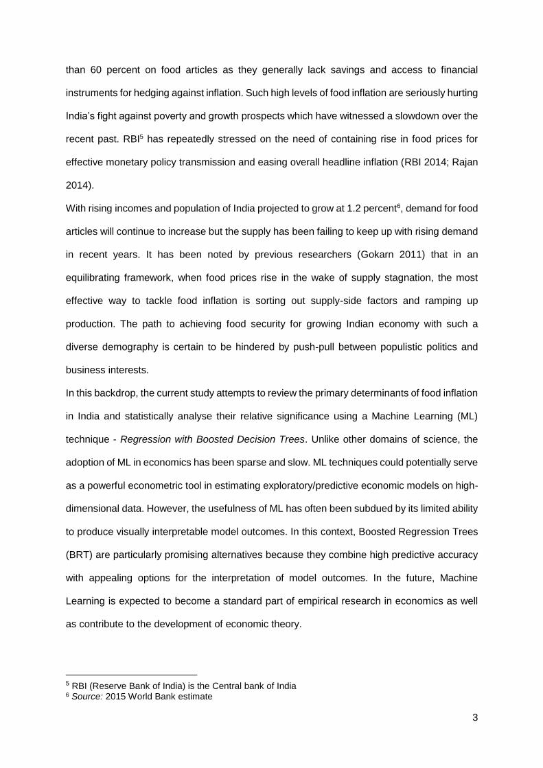
As India’s population and urban land grow in sizes, net sown area under crops has declined
after the economic liberalisation beginning from FY91 (see Fig. 5). The average size of
cultivated plots has shrunk by nearly half from 2.28 hectares in 1970-71 to 1.16 hectares in
2010-11 (Fig. 5) owing to increase in number of land holdings. Farming on such small areas
is inefficient which is further aggravated by certain state laws which limit the area of agricultural
land an individual can hold. Due to history of exploitation of peasants by landlords during
medieval period, state laws favouring strong tenancy rights make leasing agricultural land very
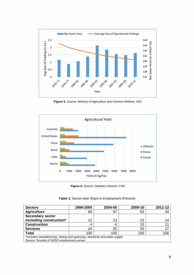
difficult in India. As compared to other major agricultural producers around the world,
agricultural yield per unit area is fairly low in India (Fig. 6). These factors along with rise of
manufacturing and service sector have caused the share of agricultural labourers in total
workforce to drop significantly over the years (see Table 1). Additionally, the long-term shifts
like increase in share of land use for export-oriented commercial crops since the liberalisation
of economy in mid-1990s has adversely affected the growth of food output (Sonna et al. 2014).
Figure 4. Impact of increased buffer stock intake on market prices (Source: Anand et al. 2016)
9
Table 1: Sector-wise Share in Employment (Percent)
Sectors 1999-2000 2004-05 2009-10 2011-12
Agriculture 60 57 53 49
Secondary sector excluding construction*
12
13
12
14
Construction 4 6 10 11
Services 24 25 25 27
Total 100 100 100 100 *Includes manufacturing, mining and quarrying, electricity and water supply Source: Rounds of NSSO employment survey
0 1000 2000 3000 4000 5000 6000 7000 8000
World
India
Brazil
China
United States
Australia
Yield (in kg/ha)
Agricultural Yield
OilSeeds
Pulses
Cereal
Figure 6. Source: Statistics Division, FAO
Figure 5. Source: Ministry of Agriculture and Farmers Welfare, GOI
137
138
139
140
141
142
143
144
0
0.5
1
1.5
2
2.5
Net
So
wn
Are
a (i
n m
illio
n h
a)
Avg
Siz
e o
f h
old
ing
(in
ha
)
Year
Net Sown Area Average Size of Operational Holdings

10
The supply-chain facilitating movement of produce from farms to fork is severely distorted with
presence of multiple intermediaries, poor logistics, price information asymmetry and addition
of brokering costs at each link. The lack of adequate transportation and storage facilities leads
to significant losses in the supply-chain. The monetary value of post-harvest loss incurred was
found out to be in excess of INR 900 billion for 2012-13 with perishable items (fruits,
vegetables and livestock produce) making up more than half of these economic losses (Jha
et al. 2015). The losses in cereals and oilseeds is mainly concentrated in farm operations with
relatively small losses in storage channels (see Table 2). However, the losses incurred in
storage networks become significantly comparable to that of farm operations in case of fruits
and vegetables.
Table 2 Harvest and post-harvest losses at national level (Source: Jha et al. 2015)
Crop type Farm operations Storage Channels Total loss
Cereals 4.37 % 0.89 % 5.26 %
Pulses 5.79 % 1.32 % 7.11 %
Oilseeds 4.73 % 0.79 % 5.52 %
Fruits 7.44 % 2.30 % 9.74 %
Vegetables 6.58 % 1.98 % 8.56 %
The Agricultural markets are fractured in themselves led by state marketing boards known as
Agricultural Produce Market Committee (APMC) which restricts farmers’ trade options only to
traders or commission agents licensed to operate in the area under a particular APMC. As per
the Indian Constitution, agricultural marketing is a state (provincial) subject. The intra-state
trading falls under the jurisdiction of state government while the inter-state trading comes
under Central government. As a result, agricultural markets are prevailed and administered
mostly under the several State APMC Acts. Until recently, a trader in northern state of Punjab
was not allowed to bid for coconuts in southern state of Kerala. This gives opportunity to
arhatiyas or local commissioning agents, the infamous intermediaries who add little or no value

11
to the supply chain and are known for exploiting farmers and charging hefty commissions on
sales, in some cases even up to 14 percent as opposed to the international norm of 0.5 percent
on such sales. In addition to low profitability, the uncertain trade policies practiced by central
and state governments discussed in the next section, further discourage farmers to invest or
specialize in advanced farming techniques.
2.4 Agricultural Trade Policies
Food inflation is a political scandal in India as it distorts the consumption basket of a common
voter. Amidst political pressure, governments respond to surge in food prices by imposing
export bans, sometimes even at state levels13. India cautiously regulates its agricultural trade
by frequently imposing import-export bans and change in duties to protect the interests of
domestic farmers, relevance of MSPs as floor prices and, of course to shield the domestic
markets from global price bouts. In the wake of 2007-08 global food price crisis, India adopted
a very restrictive trade policy including ban on exports of wheat and rice which continued till
2011. In case of pulses, for which domestic production is not sufficient, India currently prohibits
export of most of the pulses complementing this with zero import duty.
However, in events of sporadic shortages arising out of droughts etc. the delays in
announcement of policy changes to meet domestic demand with increased imports often
results in government agencies importing at much higher prices as the global market has
already factored in the existing shortage in India. The primary reason behind this recurrent
policy failure is lack of an institutional mechanism for forecasting global and domestic food
supply and prices based on which timely warnings could be issued to relevant agencies.
Consequently, central and state governments fail to coordinate and reach a timely solution
facilitating quick imports before build-up of domestic shortage. There have been instances of
temporal trade imbalance (see Chand 2010) in the past when a certain commodity was
13 For instance, in 2014, state government of West Bengal imposed a ban on shipping potatoes to other Indian states in response to escalated prices.

12
exported during the times of surplus supply at low prices and then imported back in
subsequent time periods at higher prices to meet domestic shortage, resulting in huge losses
to the exchequer.
India is a net exporter of cereals, but a major importer of oilseeds and pulses, in fact being the
largest consumer of pulses India has become the largest producer and importer of pulses as
well.
2.5 Food Inflation: Timeline
Elevated levels of persistent inflation have posed a serious macroeconomic challenge to
India’s growth prospects. The average year-on-year aggregate inflation (7.4%) and food
inflation (7.2%) were at comparable levels during FY91 to FY06, but post 2007 financial crisis
food inflation has always exceeded aggregate retail inflation by more than two percentage
points, barring two years of FY11-12 in which crude oil prices rose sharply taking fuel
component of total inflation with itself (see Fig. 1). Food prices grew at sustainable rates
during 1980s and 1990s owing to success of ‘Green Revolution’ - a combination of demand
and supply side interventions focussed on agricultural infrastructure development, farm input
subsidies and technological investments which aided in stabilizing the growth of agricultural
output at par with demand. However, as growth in agricultural output slowed after 1990s,
Indian government had to tap into buffer stocks to meet increasing food demand which kept
the food prices in check during early 2000s. This led to depletion of stocks being held in central
pool which was further accelerated with Indian government’s response to shield domestic
markets from surge in international food prices during 2007-08 (Fig. 3, Fig. 14). Eventually,
the stocks in central pool fell below the accepted norms which prompted the food authorities
to ramp the procurement causing shortage in the domestic markets. This shortage was further
aggravated by low agricultural output from drought in 2009 causing food inflation to touch
double digits during FY09-10. The effect of decline in global food prices in FY10 was not
transmitted into the domestic market as the domestic food prices grew by more than 15% in

13
that year primarily due to excessive stock hoarding in the wake of 2007-08 global food crisis.
Even though FY10-11 had a good monsoon, the food inflation didn't ease much as both the
core and aggregate inflation picked up in these years.
With a moderate gain in FY12, food prices started rising again as the household inflation
expectations remained at persistently high levels during FY10-14 (Fig. 7), a period which
witnessed surge in crude oil prices and political upheavals with state and general elections
being held in 2013-14.
Various government interventions including significant hikes in MSP, pre-election policy
announcements involving food and fertiliser subsidies and other populist measures caused
ballooning of central and state fiscal deficits. These measures not only caused inflation in the
immediate years, but also prolonged the inflationary pressures in the economy resulting into
double digit food inflation during FY13-14. With the creation of an inflationary spiral of elevated
inflation expectations14 and food inflation levels transmitting into core inflation and wages15,
the aggregate retail inflation remained at uncomfortably high levels during 2010-14 averaging
14 According to RBI (2014), a one percent increment in food inflation is followed by an immediate rise in one-year-ahead household inflation expectations by half percentage points, the effect of which persists for eight quarters. 15 The influence of Indian food inflation on price expectations and wage setting create large second-round effects on core inflation (Anand et al. 2014)
0
5
10
15
20
Sep
-06
Feb
-07
Jul-
07
Dec
-07
May
-08
Oct
-08
Mar
-09
Au
g-0
9
Jan
-10
Jun
-10
No
v-1
0
Ap
r-1
1
Sep
-11
Feb
-12
Jul-
12
Dec
-12
May
-13
Oct
-13
Mar
-14
Au
g-1
4
Jan
-15
Jun
-15
No
v-1
5
Ap
r-1
6
Infl
atio
n R
ate
(%)
One-year-ahead household inflation expectations Food inflation Headline inflation
Figure 7. Household inflation expectations (Source: RBI)

14
more than ten percent. Within the food items, the highest inflation was observed among pulses
with a three-fold rise in prices, whereas the price of overall food basket has doubled in the last
ten years.
2.6 Dynamics: Supply-Demand Mismatch
Driven by strong economic growth in late 2000s, per-capita real private consumption
expenditure in India grew annually at an average rate of 6.7 percent during FY06-FY12.
Moreover, the growth in per-capita private consumption and disposable personal income
remained significantly unaffected from the repercussions of Financial crisis in 2007-08 (see
Fig 8). However, with economic slowdown in FY13-14 demand-side pressures on food prices
eased off as growth in consumption fell below 5 percent.
The domestic demand for food has been rising continuously with an ever-increasing
population. The domestic production has failed to keep up with this persistent rise in demand
and has almost stagnated in the last five years. Domestic agricultural output grew annually at
an average rate of 0.9 percent during FY01 – FY10 (Fig. 9), whereas in the same period, the
population recorded an annual average growth rate of more than 1.5 percent. This mismatch
in demand and supply is fairly severe in the case of pulses for which consumption has risen
0%
5%
10%
15%
20%
FY92
FY93
FY94
FY95
FY96
FY97
FY98
FY99
FY00
FY01
FY02
FY03
FY04
FY05
FY06
FY07
FY08
FY09
FY10
FY11
FY12
FY13
Annual percent change in Income & Consumption
Per capita consumption expenditure
Per capita disposable personal income
Figure 8. Base 2004-05 (Source: National Account Statistics, MOSPI)

15
significantly as compared to domestic production. India has not able to meet its demand for
pulses even after imports. As a result, the per capita net availability of pulses, after
incorporating imports and exports, has fallen significantly from 25.2 kg/year in 1961-62 to 13.1
kg/year during 2000-2014, whereas cereal availability has increased in the same timeframe
(see Fig. 10).
When dealing with traded goods, it is commonly assumed that supply is perfectly elastic in
prices, with demand getting adjusted to clear markets. However, as previous studies (Kumar
0
500
1000
1500
2000
2500
-20%
-15%
-10%
-5%
0%
5%
10%
15%
20%
25%
FY91 FY93 FY95 FY97 FY99 FY01 FY03 FY05 FY07 FY09 FY11 FY13 FY15
Yiel
d (
in k
g/h
a)
Pro
du
ctio
n o
utp
ut
YoY
Fiscal Year
Domestic Agricultural output
Agricultural yield (kg/ha) Annual percent change in Production output
Figure 9. Source: DBIE, RBI; and author calculations
0
20
40
60
80
100
120
140
160
180
0
5
10
15
20
25
30
Cer
eals
(kg
/yea
r)
Pu
lses
(kg
/yea
r)
Per capita net availabilty of foodgrains in India
Pulses - per capita net availability Cereals - per capita net availability
Figure 10. Source: Economic Survey 2015-16

16
et al. 2010) on agricultural commodities have shown that when compared to own price
elasticities of demand, supply has lower own price elasticities in Indian context. The implication
of this observation is more prominent in the near-term dynamics, where the movement in
prices caused due to shift in demand is supposed to remain unaltered with supply response.
This apparent agricultural supply inelasticity16 is known to create inflationary pressures on food
prices in India as noted by Reddy (2013) along with two other supply-side reasons - one of
them is supply bottleneck which is mainly endogenous to the system, arising out of lack of
adequate investment in supply logistics and supporting mechanisms; and the other being
supply shock which is a transient endogenous factor caused primarily due to deficient
monsoon, floods or other anomalies in climate.
2.7 Pulses: Catching fire
The last few years have witnessed frequent episodes of absurdly high inflation in pulses, with
prices getting tripled in the last decade. In FY16 alone, prices of pulses increased by more
than 45 percent (Fig. 11). Over the years, the supply of pulses has failed to keep up with
increasing demand arising primarily out of higher rural household incomes and shift in dietary
patterns. In recent times, consecutive monsoon shocks of 2014 and 2015 have further
aggravated the situation and with international pulse prices at elevated levels and weak rupee,
imports failed to ease inflationary pressures.
Over the long term, this shortfall in production occurred mainly due to decline in farm area
under pulse cultivation with cultivators opting for high-yielding crops, such as rice and wheat,
which offer higher procurement prices. This has eventually led to lower yields in pulse
cultivation as it got pushed to poorly-irrigated smaller farms with low quality soils. These farms
with inadequate access to irrigation are dependent on rainfall which increases the risk of crop
failure. As unshelled pulses have a low shelf life, risk of post-harvest losses due to subpar
storage infrastructure, limited access to milling facilities and lack of government assurance for
16 In an inelastic supply system, only price but not supply adjusts to equilibrate demand.

17
procurement further discourages farmers to cultivate pulses on their land. Unlike rice and
wheat, MSPs of pulses are much lower than open market prices. Every year, procurement
prices are announced by government before the start of sowing season of pulses, just like rice
and wheat, but without any procurement being done post-harvest. The lack of buffer stock for
pulses certainly limits the ability of government to mitigate any adverse supply shock and
control price spikes. Consequently, this has led to larger dependence on international markets
which is thin and volatile in case of pulses. India had to import 5.79 MT of pulses in FY16 to
meet the shortfall. The domestic production for pulses in FY16 stood around 17 MT which is
significantly short of the estimated demand of nearly 24 MT. The issue of pulses is certainly
an important one, as India is now the largest producer, consumer and importer of pulses
globally. Unlike oilseeds which has a robust international market and involves large public and
private import houses, the global market of pulses is feeble causing absence of structured
import houses for pulses in India. This restricts the ability of Indian food management
authorities to ease persistent inflation in pulses with international trade.
2.8 Measures of Inflation in India
Currently, four measures of retail inflation (CPI) exist in India along with a wholesale price
index (WPI). However, data collection methodology is more robust for CPI compared to WPI,
Figure 11. Retail inflation in pulses based on CPI-IW; Source: CSO

18
which lacks pan-India data collection centres and fixed periodicity of surveys. Moreover, CPI
weightages are more closely related to household expenditure and reflects the true cost of
maintaining a standard of living as opposed to WPI (see Table 3). Mathematically, CPI is better
able to capture the movement in prices arising out of demand side factors as well as future
inflation expectations. Adhering to recommendations made in RBI (2014) by Expert Committee
to Revise and Strengthen the Monetary Policy Framework, RBI has started monitoring CPI
closely while framing monetary policy and adjusting interest rates. This makes CPI a
preferable measure for studying inflation in Indian scenario.
However, accessing distant past series of all-India CPI poses a difficulty as the combined CPI
which encompasses all segments of population was launched recently in January 2011 with
2010 as base year. Prior to advent of all-India CPI, four different price indices were estimated
catering to specific segments of Indian population; namely (i) CPI-IL for industrial labourers,
(ii) CPI-AL for agricultural labourers, (iii) CPI-RL for rural labourers, and (iv) CPI-UNME17 for
urban non-manual employees. Among these, CPI-IL has a wider geographic coverage and
latest base year than the other two price indices. Moreover, CPI-IL is used as a proxy of cost
of living index in the organised sector and had been a broad-based inflation indicator for the
country as a whole before the introduction of all-India CPI. RBI (2014) observed CPI-IL and
all-India CPI showing similar inflation trends making it the most suitable measure of inflation
for econometric analysis and the same has been employed in this study.
Table 3. Item-wise weights
17 CPI-UNME was discontinued permanently in 2010.
Group/Sub-group CPI-IW (Base 2001) NSSO 2011-12
household survey WPI (Base 2004-05)
Rural Urban Cereals and Products 13.48 12.1 7.4 6.28
Pulses and Products 2.91 3.3 2.2 0.72
Milk and Products 7.31 9.1 7.8 3.24
Edible Oil 3.23 3.8 2.7 3.04
Egg, Fish and Meat 3.97 3.6 2.8 2.41
Other Food 15.3 16.7 15.7 13.4
Food Total 46.2 48.6 38.6 29.09
Non-food Total 53.8 51.4 61.4 70.91

19
3. Factors driving Food Inflation in India
3.1 Monsoon dependency
The very nature of Indian economy puts in perspective significance of rains in making a good
crop year, especially southwest monsoon lasting from July to September. More than half18 of
India’s net sown area, land which is cropped at least once a year, still remains unirrigated and
relies on water that rains down from the clouds, mostly in the monsoon months. Over the time,
deviations in geographical distribution and rainfall observed during southwest monsoon have
significantly affected the agricultural output and hence food prices (Mohanty, 2014). Analysing
the historical data (between 1956 and 2010), Mohanty (2010) argues that high food prices
caused by droughts were responsible for more than three-fourths of the instances of double
digit inflation in India. A deficient monsoon builds inflation expectations and adversely affects
the production output. Empirical evidence based on data from past 25 years suggests a
positively weak correlation of 0.3 between food inflation and monsoon deviation from long term
mean in the same year, which is counterintuitive in itself (ideally, it should come negative!).
However, on segregating the drought years19, a significantly negative correlation of -0.8 is
found out between monsoon deviation and food inflation in the following year (Fig. 12).
18 Source: Ministry of Agriculture & Farmers Welfare, Government of India. 19 For the purpose of this study, year in which monsoon was deficient by more than 10 percent from long term average was considered as a drought year.
Figure 12. Food inflation based on CPI-IW (base year 2001) (Source: DBIE, RBI)
20
3.2 Minimum Support Prices
The role of MSPs in guiding food inflation is fairly large as the crops covered under MSP
constitute more than a third of all-India food consumption basket20. The MSP as a concept is
intended to be a floor for market prices but during years with substantial hikes, it eventually
ends up setting market prices directly, which is generally followed by rise in prices of key
agricultural crops (Rajan 2014; Mishra and Roy 2011). With the abolishment of practice of
announcing separate procurement prices in mid 1970s, MSPs have become minimum prices
at which FCI stands ready to buy/procure whatever quantities farmers have to offer. This
certainly has aided in excessive building of buffer stocks in central pool when hikes have been
significant.
The use of incentive schemes like MSP in boosting agricultural production may be limited as
Rajan (2014) argues that, “the gains from MSP increases have not accrued to the farm sector
in full measure on account of rising costs of inputs”. This is evident from the trend in internal
Terms of Trade21 (ToT) of agricultural commodities which has flat-lined in the recent times.
Rajan (2014) compares the approach of increasing production through hikes in MSP to “a dog
chasing its tail” - it can never catch it, as hikes in MSPs also drives input costs upwards.
However, if higher MSPs lead to higher supply of rice and wheat, which are the primary
commodities procured at MSP, then this might also result in a suboptimal mix of production,
distorted towards rice and wheat, with a reduced supply of other food commodities causing
non-cereal food inflation.
As shown in Fig. 13, an MSP-induced increment in production is necessitated by a subsidy to
a consumer to ensure post-harvest market clearing of increased cereal supply assuming no
buffer stock build-up. Thus, given the increase in fiscal burden arising out of food subsidies,
the increase in MSPs in combination with open ended procurement and PDS may elevate
20 Source: All India Weights of different Sub-groups within Consumer Food Price Index - 2012 series 21 Terms of Trade is defined as ratio of changes in input cost over the changes in the output price of agricultural commodities. A constant ToT over time implies towards a stagnant profitability, thereby, reducing incentive for investment in agriculture.

21
overall inflationary pressures in the economy even in a scenario of increased production and
declining food inflation.
3.3 International Prices and Trade Policy
After 1991, when economic reforms towards opening the economy were implemented,
agricultural markets in India have been progressively integrating with global markets.
Consequently, a shift in international food prices exert direct and indirect influence on domestic
markets through trade as well as through policy adjustments. Historically, the rising trend in
global food prices have been slowly transmitted into the domestic market (see Fig. 14) owing
to India’s cautious trade policy. A massive spike in food commodity prices was observed in
2007-08 which caused cereal prices to almost triple from their early 2000 levels droving 44
million people into poverty around the globe (World Bank, 2011). Many structural reasons
have been identified causing this politically destructive crisis22 ranging from spike in energy
22 The resulting discontent from food shortages played a significant role in causing riots and protests during 2011 Arab Spring that toppled governments first in Tunisia, followed by the Tahrir Square uprising overthrowing Egypt’s government and civil wars in many other Arab nations.
Figure 13. Impact of MSP hike on demand-supply dynamics (Source: Anand et al. 2016)

22
prices23 to increasing biofuel subsidies, and even the role of global fertiliser cartels24.The
causes may be many but the effect, however left a grave imprint on food management policy
in China and India for the subsequent years which recorded unprecedented grain procurement
and hoarding.
Overall, there appears to be low degree of correlation between global and domestic food
prices, however, on observing closely it is apparent that a higher correlation exists during
periods of low global food inflation, indicating a weak pass through during periods of high
global food inflation. This makes food prices in India less volatile than their international
counterparts, the trends, however, ultimately converges over the long-run implicating at
impermanent success of India’s agri-trade policy designed to shield domestic markets from
global price spikes. Interestingly the correlation between trends have weakened in the recent
years as the inflation in international food prices have eased, even entering the negative
territory in case of some food commodities contrary to Indian food prices which are on a
persistent rise. This weak correlation could possibly be due to large fluctuations in USD-INR
exchange rate post-2008 crisis. On comparing the domestic food index with international food
price index denominated in INR, the two indices seem to follow a similar path (Fig. 14).
23 Agriculture consumes energy both directly, through usage of diesel in operating farm machinery, and indirectly, through natural gas providing nitrogen for fertiliser production. 24 In recent studies, Gnutzmann and Spiewanowski (2014; 2016) exposed the role of fertilizer cartels in
elevating food prices. They estimated that the pure fertilizer cartel effect explained more than 60% of rise in food prices during the crisis and food prices would have been around 35% lower at the peak of crisis, has the fertilizer prices were set competitively in the absence of a cartel.
Figure 14. Movement of domestic prices with global food prices (Source: FAO; DBIE, RBI)
0
100
200
300
FY91
FY93
FY95
FY97
FY99
FY01
FY03
FY05
FY07
FY09
FY11
FY13
FY15
Pri
ce In
dex
Dollar denominated
Global Prices (in USD) Domestic Prices
0
100
200
300
FY91
FY93
FY95
FY97
FY99
FY01
FY03
FY05
FY07
FY09
FY11
FY13
FY15
Pri
ce In
dex
INR denominated
Global Prices (in INR) Domestic Prices

23
3.4 Fiscal Policies
In general, prices of agricultural commodities tend to be more responsive to macroeconomic
shocks as compared to several manufactured goods whose prices are bound by long-term
contracts (Thompson, 1998). Particularly, in a developing economy, where demand for food
is relatively inelastic and short-run price elasticities of agricultural supply is still lower, any shift
in demand arising out of macroeconomic policy change, such as fiscal or monetary stimulus,
could distort food prices significantly. A similar situation arose post 2007-08 financial crisis,
prior to which India had successfully brought down its Fiscal Deficit from almost 10 percent of
GDP in FY02 to 4 percent in FY08 (Fig. 15) following the impressive fiscal consolidation with
the passage of 2003 FRBM Act. The revenue deficit became almost null while the primary
deficit achieved a marginal surplus in FY08 (Fig. 16). But as the fears of severe unemployment
and recession grew in the wake of 2007-08 financial crisis, G7+5 countries as well as IMF
favoured a fiscal stimulus up to 2 percent of GDP as a pathway out of the feared recession.
There was a striking difference between the expansionary fiscal policies adopted in India and
other countries, for instance in China, nearly 40 percent of the fiscal stimulus was directed
toward investment in infrastructure development whereas, the Indian fiscal package was more
focussed on stimulating demand by granting direct subsidies (ranging from food, fertiliser,
energy subsidies to even flat waivers in agricultural debt25), expansionary income support
schemes like MGNERGS26 and generous pay hikes announced in Sixth Pay Commission for
state servants. These welfare and employment guarantee schemes imparted substantial
amounts of liquidity and purchasing power, particularly to rural households, boosting demand
for food items (Rakshit 2011) but with several supply bottlenecks in place, particularly,
stagnant productivity and subpar infrastructure, the situation soon got transformed into
demand-pull inflation. The withdrawal of these politically sensitive outright doles still poses a
25 Just before 2009 general elections, then ruling United Progressive Alliance (UPA) government waived the repayment of loans made to small and mid-sized farmers which, some commentators believed, helped the coalition get re-elected (Rajan 2011) 26 Mahatma Gandhi National Rural Employment Guarantee Scheme

24
challenge in winding down the deficit financing without an abrupt shock to an already fragile
growth.
3.5 Rising Input costs
Rise in farm wages inflates the cost of production and is believed to cause a wage spiral in
the economy by raising the benchmark ‘reservation wage’ - the lowest rate that workers are
prepared to accept for jobs across sectors which could possibly increase demand for food as
well (Gulati and Saini 2013). Change in farm wages disturbs the food price equilibrium in an
unbalanced way as low rural wages suppress demand only to a certain extent owing to the
relatively low income elasticity for food expenditure of rural households (which constitutes 70
-2000
0
2000
4000
6000
8000
10000
FY91
FY92
FY93
FY94
FY95
FY96
FY97
FY98
FY99
FY00
FY01
FY02
FY03
FY04
FY05
FY06
FY07
FY08
FY09
FY10
FY11
FY12
FY13
FY14
FY15
INR
bill
ion
s
Combined Government Finances
Gross Fiscal Deficit Gross Primary Deficit Revenue Deficit
Figure 16. Study of combined finances of central and state governments (Source: MOSPI)
-30%
-10%
10%
30%
50%
70%
90%
110%
130%
150%
0%
2%
4%
6%
8%
10%
12%
14%
FY91
FY93
FY95
FY97
FY99
FY01
FY03
FY05
FY07
FY09
FY11
FY13
FY15
Ch
ange
in F
isca
l def
icit
(Yo
Y)
Fisc
al d
efic
it (
as %
of
GD
P)
Combined Fiscal deficit
Fiscal deficit as % of GDP Change in Fiscal deficit (YoY)
Figure 15. Study of combined central and state governments fiscal deficit (Source: MOSPI)

25
percent of Indian population). On the other hand, rise in rural wages not only boosts demand
but also rejigs the food basket towards higher value and protein-rich items, thereby disturbing
both the demand (strong rural demand) and supply (high labour costs) side of price
equilibrium.
Farm wages have witnessed a sharp rise in the last decade, with nominal wages growing
annually at 15 percent. Nevertheless, on deflating these wages with CPI-AL, real wages still
grew at a rate of 5.3 percent per annum. Several reasons are responsible for such substantial
rise in farm wages including strong private investment spurred by an increase in commercial
credit flowing to the agricultural sector, scarcity of agricultural labourers caused by a shift in
employment pattern with labour force moving from agriculture to non-agriculture sectors,
particularly construction (see Table 1) and implementation of MGNREGS.
The role of MGNREGS in accelerating farm wage inflation is, however, still debated in the
literature. The latter phase of high growth in farm wages certainly coincided with the
implementation of MGNREGS in FY08 (see Fig. 17). Guaranteed wages under MGNREGS
may have strengthened the bargaining power of unskilled labourers in rural areas, but past
empirical studies show that only a small fraction of increase in rural wages could be attributed
to MGNREGS and that small effect, if any, is ebbing in recent years (Sonna et al. 2014).
60
80
100
120
140
160
FY91
FY92
FY93
FY94
FY95
FY96
FY97
FY98
FY99
FY00
FY01
FY02
FY03
FY04
FY05
FY06
FY07
FY08
FY09
FY10
FY11
FY12
FY13
FY14
FY15
FY16
Wag
e in
dex
Real Farm Wages
MNREGS period Real Farm Wage Index
Figure 17. Growth in real farm wages (Source: Indian Labour Bureau)

26
However, the rising trend in real MGNREGS wages suggests that its effect on rural wage
inflation will not disappear entirely; a recent study on the southern state of Kerala (Dhanya
2016), revealed that implementation of MGNREGS caused a rise in wages for certain rural
works carried out by female labour force and was accompanied with increased food
consumption expenditure.
Apart from labour costs, CACP takes other factors of agricultural production into account, as
well, while recommending MSPs to the government. Non-labour operational costs contribute
nearly half to the total cost of cultivation. The cumulative non-labour agri-input price index has
recorded more than 80 percent rise during FY05-FY16.
3.6 Shift in Food Consumption patterns
NSSO’s periodical survey on household consumption reveals that share of food in total
consumption expenditure has been declining. The observed pattern is in line with Engel’s law
which states that as the average household income rises, share of food in total expenditure
diminishes (Fig. 18) owing to relatively low income elasticity for food expenditure. Despite the
declining overall share of food in total consumption expenditure, real per capita food
consumption has been rising, especially in rural households (Rajan 2014). With rising
incomes, dietary preference has shifted in accordance to Bennet’s law towards more nutritious
and high value food items away from starchy cereals (Fig. 19). This changing preference has
resulted in high levels of inflation in pulses and other protein-rich items in the recent years.
The share of protein-rich food items, both plant and animal, in total food consumption has
risen to almost 40 percent. The prices of nutrition-rich items, including vegetables and fruits,
have recorded a higher inflation than cereals owing to suppressed growth in supply of these
items, causing a mismatch with rapidly growing demand (Mohanty 2011 and 2014). Evidence
from the literature (Rajan 2014; Gokarn 2010 and 2011) asserts that protein and high value
food items have become prominent determinants of overall food inflation in the recent times.

27
4. Statistical Modelling Framework
To study the relative significance of individual factors in explaining the inflationary trend in food
prices, a nonparametric regression ensemble has been developed using decision trees with
gradient boosting for least squares (Friedman 2001). Unlike parametric regression, supervised
machine learning techniques, such as gradient boosting, do not attempt to characterize the
relationship between predictors and response with model parameters but rather produces an
ensemble of weak prediction models, decision trees in this case, such that it improves the
0%
20%
40%
60%
80%
100%
Rural
Cereals Pulses Fruits & Veg
Meat Milk Oil
Spices Others
0%
20%
40%
60%
80%
100%
Urban
Cereals Pulses Fruits & Veg
Meat Milk Oil
Spices Others
Figure 19. Change in dietary pattern (Source: Rounds of NSSO Survey)
64 63.2 59.4 55 53.6 48.6 56.4 54.7 48.1 42.5 40.7 38.6
0%10%20%30%40%50%60%70%80%90%
100%
19
87
-88
19
93
-94
19
99
-00
20
04
-05
20
09
-10
20
11
-12
19
87
-88
19
93
-94
19
99
-00
20
04
-05
20
09
-10
20
11
-12
Rural Urban
Change in Consumption Expenditure
Non-Food
Food
Figure 18. Change in consumption pattern (Source: Rounds of NSSO Survey)

28
overall predictive performance of model (Hastie et al., 2009). Boosting, as a concept, provides
sequential learning of the predictors, where each decision tree is dependent on the
performance of prior trees and learns by fitting the residuals of preceding trees. Unlike linear
regression, regression with boosted decision trees can model complex functions by
accounting for non-linearity and interactions between predictor variables (Müller et al. 2013).
The ability of BRTs to automatically handle missing data points saves the effort of data pre-
processing. The advantage of BRTs over other predictive modelling techniques is the typical
combination of high predictive accuracy and robustness against overfitting.
In the present study, the annual inflation in retail food prices (FCPI), measured by year-on
year change in prices of food items included in CPI-IW (base 2001), is chosen as the response
variable, whereas the predictor variables27 include:
MonsDev : Deviation in rainfall received during southwest monsoon in a year from its 50-
year long-term mean
MSP : YoY change in production weighted MSP index of major food crops
FAO : YoY change in FAO price index denominated in INR
FD : Combined fiscal deficit as a percentage of total GDP in a year
FWI : YoY change in farm wage index
AgriInput : YoY change in price index of agricultural inputs constructed from WPI
ProteinExp : YoY change in ratio of private consumption expenditure on protein-rich food
items to total food expenditure
The expression of variables in percentage term brings all predictor variables as well as
response variable on the same measurement scale.
27 Selection of variables is not a priority, as BRTs tend to ignore irrelevant predictors (Elith et al.,2008).

29
4.1 Mathematical Formulation
Gradient tree boosting employs decision trees of constant size as basis functions, ℎ𝑚(𝑥),
referred to as weak learners in this context, for generating additive models as the following:
𝐹(𝑥) = ∑ 𝛾𝑚ℎ𝑚(𝑥)
𝑀
𝑚=1
wherein 𝑀 and 𝛾𝑚 represent the total number of trees employed and step length respectively.
The model is constructed in a progressive stepwise manner,
𝐹𝑚(𝑥) = 𝐹𝑚−1(𝑥) + 𝛾𝑚ℎ𝑚(𝑥)
At each step, the next decision tree ℎ𝑚(𝑥) is chosen to minimise the given loss function, 𝐿, for
the current model 𝐹𝑚−1(𝑥) and its fit 𝐹𝑚−1(𝑥𝑖):
𝐹𝑚(𝑥) = 𝐹𝑚−1(𝑥) + argminℎ
∑𝐿(𝑦𝑖 , 𝐹𝑚−1(𝑥𝑖) − ℎ(𝑥))
𝑛
𝑖=1
The initial model 𝐹0 is specified by the type of loss function used. The idea behind gradient
boosting is to solve this minimization problem numerically through steepest descent. The
steepest descent is identified as the negative gradient of the given loss function calculated at
the current model 𝐹𝑚−1,
𝐹𝑚(𝑥) = 𝐹𝑚−1(𝑥) + 𝛾𝑚∑∇𝐹𝐿(𝑦𝑖 , 𝐹𝑚−1(𝑥𝑖))
𝑛
𝑖=1
Now, the step length 𝛾𝑚 is selected by means of line search:
𝛾𝑚 = argmin𝛾
∑𝐿(𝑦𝑖 , 𝐹𝑚−1(𝑥𝑖) − 𝛾𝜕𝐿(𝑦𝑖 , 𝐹𝑚−1(𝑥𝑖))
𝜕𝐹𝑚−1(𝑥𝑖))
𝑛
𝑖=1
In addition to conventional BRTs, a simple regularisation strategy, as proposed by Friedman
(2001), has been employed to improve the accuracy of the model which scales the contribution
of each tree by a factor 𝜗, also known as learning rate:
𝐹𝑚(𝑥) = 𝐹𝑚−1(𝑥) + 𝜗𝛾𝑚ℎ𝑚(𝑥)

30
Stochastic gradient boosting, which combines gradient boosting with bagging, could further
improve the performance of model; wherein at each iteration a subsample of data is randomly
drawn (without replacement) from the available dataset (Friedman, 1999).
4.2 Model parametrization
The calibration of developed BRT model is done through the following parameters,
i. Number of trees: The number of trees/iterations determines the model complexity. A
large number of trees is recommended to exhaust the internal data structure and bring
the mean squared error to statistically acceptable levels.
ii. Learn rate / Shrinkage: Slow learning rate improves predictive performance at the
expense of increased computation time, however, smaller shrinkage values are
recommended while growing a large number of trees.
iii. Maximum nodes / splits per tree: The number of splits determines the tree complexity
and order of interactions between predictor variables. In general, a tree with k nodes
can capture interactions of order k. Hastie et al. (2009) recommends four to eight splits
for most cases.
iv. Minimum number of observations in terminal nodes: This parameter should be kept
below five for small datasets
v. Subsample fraction: The rate of subsampling decides the proportion of learn sample
to be used at each modelling iteration. Subsampling fraction close to 1 makes the
model computationally intensive, however values between 0.9 to 0.95 are
recommended when dealing with small datasets.
vi. Regression Loss criterion: Among all kinds of loss functions, the natural choice for
regression is least squares owing to its overlying computational attributes. For least
squares, the initial model 𝐹0 is specified by the mean of the target values.
31
4.3 Data
The annual data series is considered for all the variables spanning a period of 25 years starting
from FY91 to FY16. The year FY91 is chosen as a starting point for a specific reason as the
first round of reforms aimed at economic liberalisation began in 1991 which reduced state
monopoly and led to gradual integration of Indian domestic markets with global markets. Data
used in this study has been primarily imported from various official sources, viz, Reserve Bank
of India (RBI), Labour Bureau of India, Central Statistics Office (CSO), Ministry of Agriculture
& Farmers Welfare, Ministry of Finance and Open Government Data (OGD) Platform India. A
production weighted MSP index (base: FY05) has been created for major food crops including;
cereals - rice, wheat and maize; pulses - gram and tur; oilseeds - groundnut, mustard and
soybean. The annual average of global food price index (base: 2002-04) published monthly
by FAO (Food and Agricultural Organisation) is converted into rupee terms using the yearly
average of USD-INR exchange rate. Combined fiscal deficit of central and state governments
as a percentage of total GDP is considered. A farm wage index28 (base: FY05) has been
constructed by aggregating wages earned by agricultural labourers engaged in primary farm
operations, namely, ploughing, sowing, transplanting, weeding, and harvesting. The weights
used in constructing non-labour agri-input price index29 (base: FY05) have been derived from
WPI 2005 series. Relative expenditure on protein-rich items is based upon weights derived
from Private Final Consumption Expenditure30 (PFCE) at constant prices (base: 2003-05), for
both plant and animal protein based items, namely, pulses, oil & oilseeds, milk & milk products,
and meat-egg-fish (MFE).
28 The data for farm wages is available from FY91, hence YoY change could only be measured starting from FY92. 29 The non-labour agricultural inputs include agricultural electricity, light diesel oil, high speed diesel, agricultural machinery & implements, tractors, lubricants, fertilisers, pesticides, cattle feed and fodder. 30 PFCE item-wise breakup data is available only till FY13.

32
4.4 Results and Discussion
The BRT model has been constructed over 50,000 trees with a learn rate of 0.0001 and
subsample fraction of 0.95. To capture multi-variable interactions in the given small dataset,
six maximum nodes per tree are allowed and minimum number of observations in terminal
nodes is kept at three. The developed model fits the actual data quite well (see Fig. 20 and
Table 4) with a R-squared value of 99.1 percent and MSE (mean squared error) flatlining
beyond 30,000 trees (Fig. 21).
Table 4 BRT model error measures
MSE (Mean squared error) 0.00002
MAD (Mean absolute deviation) 0.00321
R-sq (R-squared) 0.99073
ROC31 (Area under curve) 0.99877
31 In machine learning, accuracy is measured by the area under the ROC (Receiver Operating Characteristics) curve, wherein the model performance is considered excellent for values between 0.9 and 1.
Figure 20. Comparison of BRT model predictions to actual data
0%
2%
4%
6%
8%
10%
12%
14%
16%
18%
FY9
1
FY9
2
FY9
3
FY9
4
FY9
5
FY9
6
FY9
7
FY9
8
FY9
9
FY0
0
FY0
1
FY0
2
FY0
3
FY0
4
FY0
5
FY0
6
FY0
7
FY0
8
FY0
9
FY1
0
FY1
1
FY1
2
FY1
3
FY1
4
FY1
5
FY1
6
Actual v/s Predicted food inflation
Actual Predicted

33
The relative importance of the predictor variables in the model is manifested via a relative
influence score of a variable, which is decided based on the number of times a variable gets
selected during splitting, weighted by the squared improvements, and averaged over all
possible trees (Müller et al. 2013). The results (see Fig. 22) indicate that none of the predictor
variables, except probably FAO, is insignificant in explaining the inflation in food prices and
contributions are fairly distributed among the variables, with MSP contributing the most to
predictive performance of BRT, followed by farm wages. Minimum support prices carry most
explanatory significance as they directly set the floor for market prices. Additionally, hikes in
MSP not only elevates the inflation expectations but combined with PDS and employment
guarantee schemes they set indirect inflationary pressures in the economy as well, by
burdening the exchequer with bloated subsidy bills and inducing a wage price spiral. Farm
Figure 21. Change in MSE with growing trees
12.05
43.26
50.79
65.91
68.99
88.96
100
0 20 40 60 80 100
FAO
Agri Input
FD
MonsDev
ProteinExp
FWI
MSP
Relative significance
Figure 22. Relative significance of explanatory variables
34
wages have recorded a sharp rise especially from FY08 onwards and during this period the
annual food inflation has averaged above 9 percent. This rise in farm wages has certainly
induced cost-push inflation in food prices by raising the overall input costs of food production
in India and stagnating the agricultural profitability at the same time. The low explanatory
significance of FAO index may in part relate to agricultural trade policies adopted by India
which prevent transmission of global food price short-term volatility into the domestic markets
and allow only long-term trend in global food prices to be captured into the recommendations
made by CACP for setting MSPs.
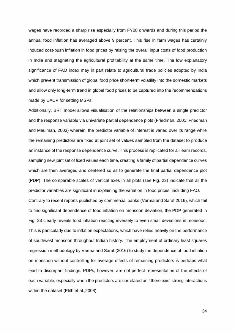
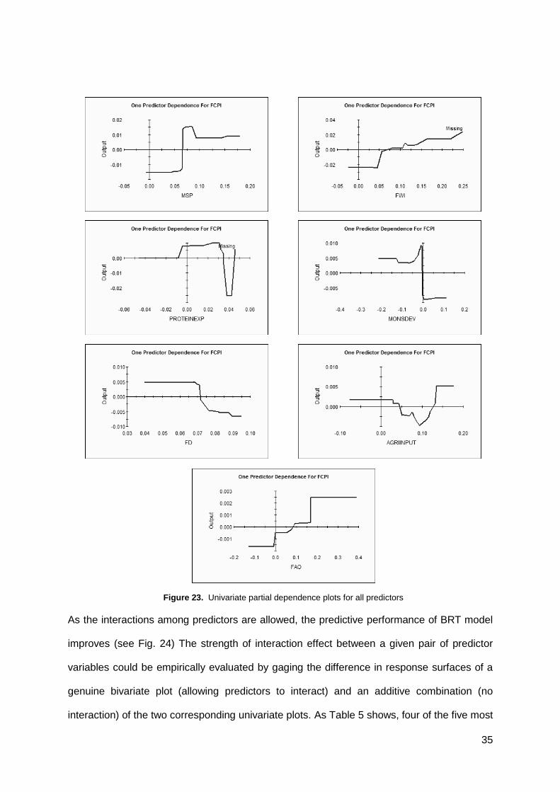
Additionally, BRT model allows visualisation of the relationships between a single predictor
and the response variable via univariate partial dependence plots (Friedman, 2001; Friedman
and Meulman, 2003) wherein, the predictor variable of interest is varied over its range while
the remaining predictors are fixed at joint set of values sampled from the dataset to produce
an instance of the response dependence curve. This process is replicated for all learn records,
sampling new joint set of fixed values each time, creating a family of partial dependence curves
which are then averaged and centered so as to generate the final partial dependence plot
(PDP). The comparable scales of vertical axes in all plots (see Fig. 23) indicate that all the
predictor variables are significant in explaining the variation in food prices, including FAO.
Contrary to recent reports published by commercial banks (Varma and Saraf 2016), which fail
to find significant dependence of food inflation on monsoon deviation, the PDP generated in
Fig. 23 clearly reveals food inflation reacting inversely to even small deviations in monsoon.
This is particularly due to inflation expectations, which have relied heavily on the performance
of southwest monsoon throughout Indian history. The employment of ordinary least squares
regression methodology by Varma and Saraf (2016) to study the dependence of food inflation
on monsoon without controlling for average effects of remaining predictors is perhaps what
lead to discrepant findings. PDPs, however, are not perfect representation of the effects of
each variable, especially when the predictors are correlated or if there exist strong interactions
within the dataset (Elith et al.,2008).
35
As the interactions among predictors are allowed, the predictive performance of BRT model
improves (see Fig. 24) The strength of interaction effect between a given pair of predictor
variables could be empirically evaluated by gaging the difference in response surfaces of a
genuine bivariate plot (allowing predictors to interact) and an additive combination (no
interaction) of the two corresponding univariate plots. As Table 5 shows, four of the five most
Figure 23. Univariate partial dependence plots for all predictors

36
important pairwise interactions include MSP and FWI, the two most relevant predictors. The
strong interaction between farm wages and protein expenditure reinforces the case of inflation
driven by boost in rural consumption amidst rising farm wages.
Table 5 Pairwise Interaction Score
All possible pairs of variables are exhausted to arrive at the overall interaction strength of each
predictor variable, which is expressed on a cumulative percent scale. MSP that captures long
term trend in global food prices as well as labour and non-labour input costs emerges with the
highest interaction score and FAO with the least (see Table 6). The two most significant
predictors, MSP and FWI, also have the highest overall interaction strength. The interaction
between these two variables could be visualized with joint partial dependence plot (Fig. 25).
32 Expressed on the percent scale, pairwise score reflects the contribution of the interacting pair normalized to the total variation in the output response.
Predictor I Predictor II Pair interaction score32
MSP MonsDev 12.4
FWI ProteinExp 11.9
MSP FD 7.0
MSP FWI 6.3
MonsDev ProteinExp 6.2
0.9
0.92
0.94
0.96
0.98
1
2 3 4 5 6 7
R-s
qu
ared
Tree complexity
Figure 24. Model performance and Tree complexity

37
Partial dependence plots for other pairs with high interaction scores (from Table 5) are
displayed in Fig. 26 (a-d).
33 As an example, the overall interaction score of MSP indicates that around 23 percent of the total variation in food prices is attributable to interaction of MSP with other predictor variables.
Table 6 Overall interaction strength of variables
Predictor MSP FWI MonsDev ProteinExp FD AgriInput FAO
Score33 23.39 20.94 19.51 17.76 9.56 8.44 1.77
Figure 25. Bivariate partial dependence plot for MSP and FWI

38
(a) Partial dependence plot for MSP and MonsDev (c) Partial dependence plot for MSP and FD
(b) Partial dependence plot for FWI and ProteinExp (d) Partial dependence plot for ProteinExp and MonsDev
Figure 26. Bivariate partial dependence plots for top interacting pairs

39
5. Policy Implications - The Way Forward
The challenge is to ensure food and nutritional security for growing Indian population with
rising incomes as land and water resources continue to become more scarce. The demand-
pull inflationary pressure on food prices is expected to increase as the economic growth picks
up in the coming years. The obvious answer lies in raising the agricultural productivity and
meet international standards through adoption of advanced agronomic technologies and
investment in sustainable farming practices. However, the growing dependence on
productivity for raising production to meet domestic demand might not help in easing
inflationary pressures in the short to medium term and may cause prices to rise even more as
introduction of new technologies increases the average cost of production during adoption
years. This might lead to a situation where inflation in food prices would sustain in a period of
rising agricultural output. That said, India certainly possess the ability to emerge as a multi-
product agricultural powerhouse backed by its diverse topography, climate and soil, and to do
so, India need to invest massively in building dense agri-supply lines, advanced agro-
processing capabilities and organized retailing. A synergetic partnership needs to be
developed between public and private players. Full relaxation in FDI limits in organized
retailing and marketing of food products announced in the Union Budget FY16-17 is certainly
a step in the right direction. This partnership could be further strengthened by franchising local
shops to act as extended outlets of organized retailers. The risk of hoarding and black
marketing by these new and already existing private players should be addressed with
establishment of a national market regulator for food commodities. The primary function of any
market is efficient price-discovery and agricultural markets in India are marred with frequent
price manipulations, excessive middlemen commissions and poor competitiveness. The
recent dilution of APMC act with launch of NAM (National Agricultural Market) - a pan-India
electronic trading portal aggregating APMCs and other market yards across states is a
welcome move towards creating a unified national market for agricultural commodities.
Similarly, several archaic laws need to be revisited to increase competitiveness in domestic

40
markets, such as Essential Commodities Act, 1955 which discourages farmers and traders
from investing in cold storages and warehousing facilities. Market-based reforms would not
only reduce the spread between wholesale and retail food prices but would also improve the
distressed socio-economic condition of farmers in India.
The rising farm wages is a positive sign and going forward, the focus should certainly not be
on stalling this rise but rather on bringing down the pay-productivity gap. High agricultural
labour productivity is essential for supplementing the higher demand arising out of increase in
wages. The desired productivity move is achievable through investment in mechanization and
extension of farms. Laws prohibiting farm land-lease markets needs to be reformed so as to
create agricultural plots of economically viable size. Intensive capital requirements of
mechanization could be addressed by enabling village panchayats in leasing farm machines.
A symbiotic partnership could be struck with expansion of MGNREGS in agriculture, wherein
a part of the wage on farm is paid by the government.
The Indian government needs to set up a strong institutional forecasting mechanism that could
send demand and price signals to the farming community before sowing season, giving
farmers the scope to scale up the production in accordance with expected demand.
Additionally, this proposed mechanism could act as an early warning system for FCI in order
to prepare for supply shortfall through international trade. The existing food management
policy needs some big reforms starting with uncoupling of competing objectives served by
procurement at MSPs and implementation of a dynamic buffer policy - timely release of food
grains from the central pool into the open market in a year of subpar production and increasing
domestic procurements, to replenish depleted buffer stocks, only during years with surplus
production. The stocks in central pool should certainly not be allowed to overshoot the
prescribed norms, unless there is a forecast of food crisis ahead. Adhering to buffer stock
norms might not only ease food inflation34 but also certainly reduce the burden on exchequer
34 Anand et al. 2016 estimates that a reduction in cumulative buffer stock intake of rice and wheat by
15 mn MT and 20 mn MT respectively during FY07-FY13 would have caused food inflation to decrease by about half percentage points per year.

41
of procuring, storing and maintaining excess stocks, thereby helping the cause of fiscal
consolidation. A renewed Indian government’s commitment to fiscal consolidation, with a
central fiscal deficit target of 3.5 percent of the total GDP for FY17, is commendable and would
certainly support the disinflation process going forward. However, the current mechanism of
administered price setting via MSPs and government interventions, through subsidies and
differentiated tariffs, distort markets to an extent of suboptimal price discovery, thereby
hindering transmission of implemented monetary and fiscal policies in the real economy,
particularly in rural areas.
The efficacy of MSP hikes to act as production incentive becomes questionable in itself as
with inflationary effects of cost-indexed MSP on farm input costs and subsidies on the same
farm inputs, the situation soon turns into ‘a dog chasing its own tail’. There is a need to
evaluate whether an exclusive policy - providing price support for output or subsiding inputs -
would be a sufficient stimulus for agricultural production. The principal role of MSPs should be
the alignment of domestic prices along the long-term trend in international prices. Volatility
and price spikes in global food prices is certainly not in the hands of any single nation, and a
globally integrated Indian economy can make the most of it by developing a pro-active neutral
trade policy (for both consumers and producers) along with a variable tariff structure, rather
than outright bans on exports or imports.
The shift in dietary pattern toward pulses and other protein-rich items is certainly a welcoming
sign, but to avoid a ‘calorie catastrophe’, India needs to develop and adopt sustainable farming
techniques. There is a need to involve public agricultural research institutes and seed
companies to develop short duration, high-yielding and pest-resistant varieties of pulses which
are suitable for inter cropping and mixed cropping in arid conditions. Government needs to
offer remunerative procurement prices for pulses, which would not only incentivise farmers
with small un-irrigated plots but would also encourage cultivators with access to capital and
irrigation to invest in pulses. The recently launched national mission (PMKSY) to expand
cultivable area under irrigation and improve farm productivity is a welcome step forward in this
regard. In addition to their nutritional advantage, pulses have low carbon and water footprints

42
which make them essential to development of sustainable farming system. The increase in
MSPs needs to complemented with procurement of pulses by FCI at the announced MSPs,
similar to rice and wheat. The recent announcement by Indian government to create a buffer
stock of 2 MT of pulses would certainly help farmers and act as a national protein security-net
during the time of crisis. As a next step, the Indian government should explore inclusion of
pulses in PDS for ensuring nutrition security to the poor.
The ability of Indian government to bring in major agricultural policy reforms and build
synergetic investment partnerships with private players would not only determine the trajectory
of food inflation in the coming years but also have a lasting effect on agricultural growth and
ultimately, rural poverty rate.
Supplementary Material
The dataset for replication of results presented in this study could be accessed at
http://dx.doi.org/10.7910/DVN/JUNBRQ.

43
References
1. Anand, R., Ding, D., & Tulin, V. (2014). Food inflation in India: The role for monetary
policy. IMF Working Paper No. 14/178
2. Anand, R., Kumar, N., and Tulin, V., Understanding India's Food Inflation: The Role
of Demand and Supply Factors (January 2016). IMF Working Paper No. 16/2.
3. Chand, R., 2010. Understanding the nature and causes of food inflation. Economic
and Political Weekly, pp.10-13.
4. Dhanya, V., 2016. Implications of MGNREGS on Labour Market, Wages and
Consumption Expenditure in Kerala. RBI Working Paper
5. “Economic Survey 2015-16”, 2016, Ministry of Finance, Government of India
6. Elith, J., Leathwick, J.R. and Hastie, T., 2008. A working guide to boosted regression
trees. Journal of Animal Ecology, 77(4), pp.802-813.
7. Friedman, J.H., 2001. Greedy function approximation: a gradient boosting machine.
Annals of statistics, pp.1189-1232.
8. Friedman, J.H., 2002. Stochastic gradient boosting. Computational Statistics & Data
Analysis, 38(4), pp.367-378.
9. Friedman, J.H. and Meulman, J.J., 2003. Multiple additive regression trees with
application in epidemiology. Statistics in medicine, 22(9), pp.1365-1381.
10. Gulati, A., Gujral, J., Nandakumar, T., Jain, S., Anand, S., Rath, S. and Joshi, P.,
2012. National food security bill: Challenges and options. Discussion Paper, (2),
CACP, Ministry of Agriculture, Government of India. New Delhi
11. Gulati, A. and Saini, S., 2013. Taming food inflation in India. Discussion Paper, (4),
CACP, Ministry of Agriculture, Government of India. New Delhi.
12. Gnutzmann, H. and Spiewanowski, P., 2014. Did the Fertilizer Cartel Cause the Food
Crisis?. Available at SSRN 2534753.
13. Gnutzmann, H. and Spiewanowski, P., 2016. Fertilizer Fuels Food Prices:
Identification Through the Oil-Gas Spread. Available at SSRN 2808381.
14. Gokarn, S., 2010. ‘The price of protein’. Monthly Bulletin, Reserve Bank of India,
November 2010.
15. Gokarn, S., 2011. ‘Food Inflation: This Time it’s Different’ Monthly Bulletin, Reserve
Bank of India, January 2011.
16. Gokarn S., 2011. “Food Inflation – This Time It’s Different”, Kale Memorial Lecture at
the Gokhale Institute of Politics and Economics, Pune, 9 December 2011.
17. Hastie, T., Tibshirani, R. & Friedman, J.H., 2009. The Elements of Statistical
Learning: Data Mining, Inference, and Prediction. Springer, New York.
18. Jha, S.N., Vishwakarma, R.K., Ahmad, T., Rai, A. and Dixit, A.K., 2015. Report on
assessment of quantative harvest and post-harvest losses of major crops and
commodities in India. ICAR-All India Coordinated Research Project on Post-Harvest
Technology, ICAR-CIPHET, PO-PAU, Ludhiana.
19. Kumar Praduman, P. Shinoj, S.S. Raju, Ankani Kumar, Karl M. Rich, and Siwa
Msangi, 2010, “Factor Demand, Output Supply Elasticities and Supply Projections for
Major Crops in India,” Agricultural Economics Research Review, Vol. 23, pp. 1-14.
20. Macroeconomics, Agriculture, and Exchange Rates. Edited by P. L. Paarlberg,
Robert G. Chambers. Westview Press. 1988.

44
21. Mishra P. and Roy D. (2011), ‘Explaining Inflation in India: The Role of Food Prices’,
Indian Policy Forum, volume 8.
22. Mohanty, D. (2010). ‘Perspectives on inflation in India’. Speech delivered at the
Bankers Club, Chennai, on 28 September 2010.
23. Mohanty, D. (2011). ‘Changing inflation dynamics in India’. Speech delivered at the
Indian Institute of Technology Guwahati (IITG) on 3 September 2011
24. Mohanty, D (2014)., ‘Why is recent food inflation in India so persistent?’. Speech
delivered at the annual Lalit Doshi Memorial Lecture, Xavier’s Chapter, delivered at
the St. Xavier’s College, Mumbai, 13 January 2014
25. Müller, D., Leitão, P.J. and Sikor, T., 2013. Comparing the determinants of cropland
abandonment in Albania and Romania using boosted regression trees. Agricultural
Systems, 117, pp. 66-77.
26. Rajan, Raghuram, 2011. Fault lines: How hidden fractures still threaten the world
economy. Princeton University Press.
27. Rajan, Raghuram, 2014, “Fighting Inflation”, Inaugural Speech at FIMMDA-PDAI
Annual Conference 2014, on February 26, 2014 at Mumbai.
28. Rakshit, M., 2011. Inflation and Relative Prices in India 2006-10: Some Analytics and
Policy Issues. Economic and Political Weekly, 46(16), pp.41-54.
29. Reddy, YY (2013). Economic Policies and India's Reform Agenda- A New Thinking.
Orient Blackswan
30. Reserve Bank of India, 2014, “Report of the Expert Committee to Revise and
Strengthen the Monetary Policy Framework,” January.
31. Saini, S. and Kozicka, M., 2014. Evolution and Critique of Buffer Stocking Policy of
India. Indian Council for Research on International Economic Relations (ICRIER).
Working Paper, (283).
32. Sonna, T., Joshi, H., Sebastin, A. and Sharma, U., 2014. Analytics of food inflation in
India. RBI Working Paper Series 10/2014
33. Thompson, Robert L (1988). Chapter 7. US Macroeconomic Policy and Agriculture.
34. United Nations 2014, Millennium Development Goals Report
35. Varma, S. and Saraf, N., 2016. India: Busting the monsoon and food price inflation
myth. Asia Economic Monthly, Nomura, 10 June 2016, pp. 28-33
36. World Bank 2011, Food Price Watch, Issue February 2011, The World Bank Group


![Understanding Machine Learning Model Expertisec4dm.eecs.qmul.ac.uk/horse2017/HORSE2017_Wagstaff.pdf · Understanding Machine Learning Model Expertise ... [Ortega et al., 2001] !](https://img.dokumen.tips/doc/110x75/5aea382f7f8b9a90318b5720/understanding-machine-learning-model-machine-learning-model-expertise-ortega.jpg)