Embed Size (px)
Citation preview

WORKING PAPER 2016
UnderstandingDollarization: aKeynesian/KaleckianPerspectiveMarco MissagliaJuly 2020
POST-KEYNESIAN ECONOMICS SOCIETY

1
Understanding dollarization: a Keynesian/Kaleckian perspective
Marco Missaglia, Università di Pavia, Italy ([email protected])*
July 2020
Abstract
What does “dollarization” mean in a world of endogenous money, i.e. a world where money is
not (only) created by printing pieces of paper, but (mainly) by making loans? Is it true that
dollarization only constitutes a limitation of sovereignty in the short run (making it harder to run
standard stabilization macro policies) or can it slow the growth process of a country? The paper
builds a theoretical, Keynesian-Kaleckian growth model for a dollarized economy in a framework
of endogenous money to answer these questions. We will show that, ceteris paribus, the steady-
state medium-term growth rate of a dollarized economy is lower than that of a country with its
own currency. We will also show that a dollarized economy is more likely to be unstable than an
economy with its own currency, in the specific sense that, everything else being equal, it is more
likely for a dollarized economy to fall into a debt trap.
JEL classification: E12, F41
1. Introduction
Ponsot (2019) reminds us that in 1983 the Israeli Minister of Finance had to resign after having
proposed to replace the Israeli currency with the US dollar. Those times are over and nowadays
dollarization is not a taboo anymore. Following the taxonomy proposed by Ponsot (2019), in
some countries dollarization is partial and de facto, meaning that the local currency coexists with
the US dollar and the latter does not constitute a legal tender; in other countries, dollarization is
integral and, again, de facto (Zimbabwe, for example); then there is the case of Guatemala, where
dollarization is de jure but the local currency (quetzal) is also a legal tender; finally, the most
known cases of “full” dollarization, integral and de jure (Ecuador, El Salvador).
* Many thanks to Elena Molho, Gennaro Zezza, Jan Toporowsky and Giorgio Rampa for useful suggestions. Errors are mine.

2
The rise of neoliberalism and the emergence of the Washington consensus in the ‘80s made this
change possible: dollarization was supposed to accelerate the integration in the global financial
market and restrict the possibility for the dollarized economy to put in place active
macroeconomic policies – the best and most direct way to import fiscal and monetary
“discipline”. In their review of its pros and cons, Rochon and Seccareccia (2003) help us
understand that according to the mainstream the costs of dollarization are essentially short run,
whereas its benefits materialize in the medium to long run. It is true that the exchange rate
ceases to be a potentially important adjusting variable1 and room to conduct fiscal and monetary
policies to soften the violence of the business cycle is restricted. However, dollarization is
supposed to a) lower inflation (and then stimulate domestic savings and, in the world of Say’s
law, domestic investment as well); b) eliminate the exchange rate risk and then boost capital
inflows and c) lower the interest rate and then reduce the weight of public debt’s service. In
short, domestic (private and public) savings would be stimulated by dollarization, and foreigners
would bring more money into the dollarized economy. All in all, the dollarized economy should
return to a sustained growth path thanks to dollarization.
The views expressed by the authors contributing to the important volume on dollarization edited
by Rochon and Seccareccia (Rochon and Seccareccia, 2003) are a lot more skeptical on the
benefits of dollarization. More than that, and more recently, even the idea that exiting
dollarization should be good for growth and development was proposed (Paredes, 2017).
Perhaps, the neater argument against dollarization is that elaborated by Izurieta (Izurieta, 2003)
through the help of a simulated Stock Flow Consistent (SFC) macroeconomic model. Assume
some balance of payments shock occurs, for instance a shortage of export demand. The current
account will suffer and, in a demand-led system, GDP and the fiscal revenue will both diminish.
In a dollarized economy, the exchange rate cannot adjust to reduce the trade imbalance and the
public sector cannot obtain “fresh” liquidity from the central bank. The dollarized economy is
then left with two options only. Either the government resorts to issuing debts or it reduces public
spending. The first “solution” is likely to be unstable, since the cost of debt servicing will further
1 According to the former Ecuadorian president, Rafael Correa (2019), the exchange rate is “the most important adjusting variable in a developing economy”.

3
feed the fiscal imbalance and, to the extent that the newly issued debt is in the hands of
foreigners, the current account will keep worsening. The second option would lead to a stable
solution, but this would be achieved thanks to (at the price of) an economic depression. In a
sense, Izurieta’s model is an application to a dollarized economy of the well-known balance of
payments constrained growth model proposed by Thirlwall2.
The idea of this paper is to propose a further reflection of dollarization through an extension
(rather than an application) of Thirlwall’s model. The extension is two-fold. First, it is to be
realized that dollarization as such does not change the endogenous nature of money. Money is
not (only) created by printing pieces of paper, it is (mainly) created by making loans. It follows
that money is endogenous everywhere, regardless of whether a country has its own currency or
not. The banking system in a dollarized economy, as it is the case in any other economy, may and
does create deposits ex-nihilo each time making loans to the economy is perceived as profitable
(even if, obviously, the deposits created by banks in a dollarized economy carry a greater risk for
these banks to run out of liquidity3). After having extended the loan, banks look for funds and,
for the private banking system as a whole operating in an economy with its own currency, the
usual source of funding is the central bank4. The “central bank” of a dollarized economy is the
rest of the world, since in such a case reserves are to be borrowed from abroad5. As we will see,
this is a huge and crucial difference, but money is endogenous in both cases. It must be
emphasized, then, that in principle it is not true, as it is often believed (for instance see also
Dullien, 2009) that the central bank of a dollarized economy cannot create money ex-nihilo to
the benefit of the domestic government. So, clarifying what dollarization truly means in a
2 Among the several papers on this topic, a useful reflection can be found in Thirlwall (1997) 3 As stressed by the World Bank in a report on West Bank and Gaza (World Bank, 2008), this in itself could restrain the creation of loans needed in a growing economy. This simple observation would be enough to understand why dollarization may slow medium-term growth, but in this paper we are going to use a different argument 4 For a single bank, the other sources of funds are deposits and the interbank market. 5 Central banks in dollarized economies may only create reserves ex-nihilo and lend them to private banks to the extent they are willing to accept to increase national foreign debt, since they cannot print a piece of paper having the status of legal tender. This makes them basically unable to control the interbank (“overnight”) rate and then the overall structure of intertest rates. Therefore, prevailing interest rates in dollarized economies are largely affected by the “world” interest rate, i.e. the rate applied on funds borrowed from abroad. In other words, the interest rate is again exogenous (as claimed by the theory of endogenous money) but, instead of being decided by the domestic policymaker, it is decided by the foreigners. It is a huge difference.

4
framework of endogenous money is an important purpose of this paper. The other extension to
the standard Thirlwall model regards the source of the external constraint a dollarized economy
must deal with. In very general terms (for both dollarized and non-dollarized economies), the
weaker the productive structure, the tougher the external constraint: domestic demand stimuli
are bound to translate into current account troubles. In a dollarized economy, however, the
current account may worsen and the stock of foreign debt increase simply because, for any given
productive structure and any given configuration of the government fiscal policy, people increase
their preference for cash (see section 2). In other words, we will see that if people increase their
preference for cash (withdraw money from their bank account and keep it into a safe at home),
nothing will happen in a country with its own currency, whereas the balance-of-payments-
constrained growth rate of a dollarized economy will lower.
The aim of this paper is then to build a theoretical growth model for a dollarized economy in a
framework of endogenous money. We will show that, ceteris paribus, the steady-state medium-
term growth rate of a dollarized economy is lower than that of a country with its own currency.
We will also show that a dollarized economy is more likely to be unstable than an economy with
its own currency, in the specific sense that, everything else being equal, it is more likely for a
dollarized economy to fall into a debt trap.
What the experience of dollarized economies shows is that in times of crisis people preference
for cash (the legal tender) as a store of value drastically increases (see Acosta and Guijarro, 2018,
p. 236-37, for an illustration of the Ecuadorian case). Scared people just go to ATM or the bank
counter and withdraw, and then hold money (cash) under the pillow or in a safe at home. The
legal tender is (perceived to be) like gold – a safe asset to be held in times of troubles. Referring
to “people” or “households” is not very satisfactory, and one should incorporate a class
dimension in a serious discourse on dollarization. The way rich people and the middle class react
to uncertainty is not the same. The latter increases its preference for the legal tender, whereas
the former strengthen their preference for holding foreign assets (“capital flights”). This is an
extremely interesting and important aspect of dollarization. However, this is beyond the scope
of the paper, where we intend to present a first theoretical reflection on this topic and
concentrate on the growth implications of “people” having a more or less pronounced preference

5
for cash as a store of value. For this reason, and to keep the model analytically tractable, income
distribution will be taken as given. Keeping in mind that in the post-Keynesian tradition income
distribution and inflation are strongly related to each other – the latter being the outcome of the
conflict over the former6 - inflation will be treated exogenously as well. Taking the (given)
inflation rate to be zero is not only (and not mainly) justified by some need of analytical
tractability. What we really want is to compare two economies with the very same essential
macro features (same inflation and real exchange rate, same income distribution, etc.) and this
way understand the “pure” implications of having an own currency or not on the growth path of
the system. In other words, imagine that dollarization has properly done its job, i.e. stabilized
inflation in the dollarized country at the same (or comparable), low level as that prevailing in
other economies (taking this level to be zero is just a matter of simplicity): once this is done, what
are the consequences of remaining dollarized in terms of medium-term growth and likelihood of
being hit from some financial mess (falling into a debt trap)?
2. Preference for cash
In a world of endogenous money - the world as it is, where money is created by making loans and
not (only) by printing pieces of paper - being “dollarized” only constitutes a limitation to the
extent that people are willing to hold some cash (pieces of paper) as a store of value. Indeed,
should people be happy with their bank deposits, the limitation of sovereignty associated to
dollarization would be a purely formal one: you cannot print a piece paper people are just not
willing to hold. In a cashless (better: in a framework where cash never constitutes a store of
value), endogenous money world, being dollarized or not would not make any relevant
difference.
Cash (as a store of value), however, does exist. Especially in time of troubles, people go to the
ATM or the bank counter and withdraw cash to be held in some safe at home. This is of course a
perfectly rational behavior. When you are scared and think your bank and/or the banking system
as a whole is going to collapse or simply suffer, you want cash. You want the legal tender under
your pillow. Even more so when the legal tender is the US dollar, a powerful currency trusted
6 Weintraub (1958) and Rowthorn (1977) are the pioneers of this “conflicting claim” view on inflation.

6
around the world. It is true that faced with the fear of some financial troubles, people increase
their preference for cash everywhere, both in dollarized and non-dollarized economies. However,
there is a huge difference between the two cases. In a non-dollarized economy, people know it
will be always possible for monetary authorities to satisfy the increased demand for cash by just
printing more of it. In a dollarized economy, people know this is not possible and then the extra-
demand for cash will have to be met by borrowing from abroad. Will the country be able to get
these loans in the first place? What will be the conditions attached to the loans? Will the economy
suffer from being more indebted toward the rest of the world? These are the reasons why,
instead of “waiting too long” (waiting for the concrete occurrence of some unhappy event) to
withdraw cash, people in a dollarized economy, compared to those living in non-dollarized
countries, are likely to keep “on average” a higher fraction of their liquid wealth in the form of
cash. Let us call α, with 0 < α < 1, the fraction of their liquid wealth households want to hold in
cash. What we are saying is that on average α is higher in dollarized than in non-dollarized
economies. What are the implications of having α at different, exogenous levels? This is what we
are going to discuss in the basic model presented in sections 3 and 4. After all, the very fact of
wishing to hold cash (which has to be borrowed from abroad) rather than deposits (which have
not) might well increase the stock of foreign debt and worsen the current account, in a potentially
destabilizing spiral we want to study and understand carefully.
3. The basic model in the short-run
Loosely speaking, the model we are going to build is Keynesian/Kaleckian. Keynesian, because
the level of activity fundamentally depends on entrepreneurs’ expectations; Kaleckian, because
at the macro level entrepreneurs end up earning what they decide to spend in the first place.
Short run
A minimalist structure to think about dollarization is illustrated in the Stock Matrix (SM) and Flow
Matrix (FM) below. In order to focus on dollarization, there are no securities and households may
only hold their financial wealth either in cash (the legal tender, H) or in a bank deposit, D. Without
losing any generality, we assume the interest rate on deposits to be zero.

7
SM (dollars)
Households Firms Banks RoW TOTAL
Deposits D -D 0
Cash H -H 0
Loans -L L 0
Foreign loans -Lf Lf 0
Capital pK pK
TOTAL V 0 0 -NFA V = pK + NFA
In this open economy, households’ nominal wealth (V) is the sum of the value of the capital stock
(pK) and the net foreign asset position (NFA) of the country. The latter, in turn, is the difference
between cash holdings (H, a liability for the Rest of the World in our dollarized framework) and
net foreign debt (Lf, which in principle may be either positive or negative; together with deposits,
foreign debt is the counterpart of banks’ loans to firms, L). So:
𝑉 = 𝑃𝐾 + 𝐻 − 𝐿𝑓
Using the definitions v = V/PK (normalized real wealth or wealth-to-capital ratio), h = H/PK
(normalized real cash in the hand of households) and lf = Lf/PK (external debt-to-capital ratio),
the above accounting identity may be written as
𝑣 = 1 + ℎ − 𝑙𝑓 (1)
In each moment in time (in the “short-run”), the stock of existing wealth is what it is. It is given
by the history of the economy. Obviously, it evolves over time (in the “medium-run”). The fact
that V (and then v) is given in the short-run has an important implication: the (short-run)
variations of h and lf must be the same. The economic rationale is very simple. If people go to the
ATM or the bank counter and withdraw (h goes up), the only way for the banking system of a
dollarized economy to satisfy this increased demand for cash is to borrow it from abroad (lf

8
increases by the same amount). This certainly produces real effects because the interest bill to
be paid to the foreigners rises and GNI correspondingly falls, but in the short-run the economy is
becoming neither richer nor poorer as a consequence of the decision of people to hold their
wealth under the pillow rather than in a bank deposit. The same concept may be expressed in a
different way, which will reveal convenient for a deeper grasping of the dynamic analysis we will
undertake at a later stage. We know α represents the fraction of their (liquid) wealth people wish
to hold in cash, i.e. H = αV. Normalized real cash in the hand of households, h, may then be
expressed as h = αv. Hence, it is possible to rewrite (1) as
𝑣 =1−𝑙𝑓
1−𝛼
or, re-arranging
𝑙𝑓 = 1 − 𝑣(1 − 𝛼) (1bis)
This formulation will reveal useful to develop our dynamic analysis and makes it clear that in the
short-run, for a given level of v, any increase in people preference for cash translates into a higher
external debt-to capital ratio. To put the same thing differently: for a given level of v, a country
becomes a debtor (lf › 0) when α > (v – 1)/v.
FM (dollars)
Hous Firms Banks RoW TOT
Curr Cap Curr Cap Curr Cap
CONS -pC pC 0
INV pI -pI 0
EXP pX -pX 0
IMP -M M 0
[memo] Nominal GDP = pC+PI+pX –M = W + Pf + Pb + i*Lf
Int on L -iL iL 0
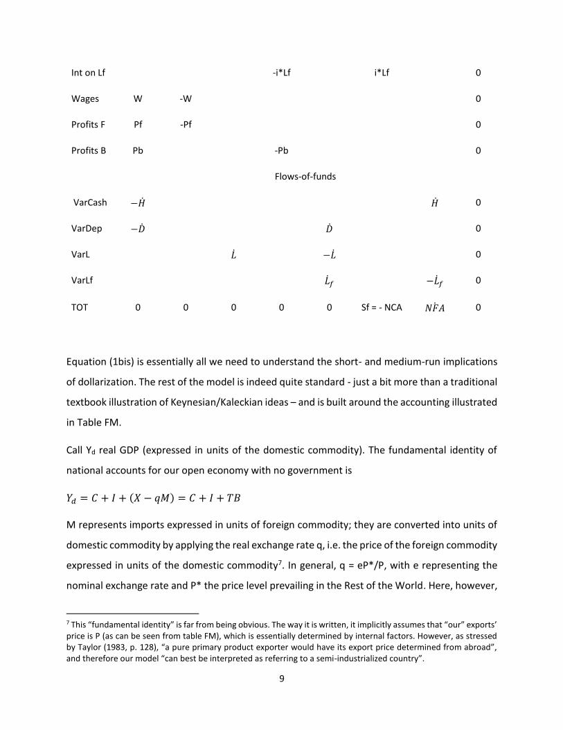
9
Int on Lf -i*Lf i*Lf 0
Wages W -W 0
Profits F Pf -Pf 0
Profits B Pb -Pb 0
Flows-of-funds
VarCash −�̇� �̇� 0
VarDep −�̇� �̇� 0
VarL �̇� −�̇� 0
VarLf �̇�𝑓 −�̇�𝑓 0
TOT 0 0 0 0 0 Sf = - NCA 𝑁𝐹𝐴̇ 0
Equation (1bis) is essentially all we need to understand the short- and medium-run implications
of dollarization. The rest of the model is indeed quite standard - just a bit more than a traditional
textbook illustration of Keynesian/Kaleckian ideas – and is built around the accounting illustrated
in Table FM.
Call Yd real GDP (expressed in units of the domestic commodity). The fundamental identity of
national accounts for our open economy with no government is
𝑌𝑑 = 𝐶 + 𝐼 + (𝑋 − 𝑞𝑀) = 𝐶 + 𝐼 + 𝑇𝐵
M represents imports expressed in units of foreign commodity; they are converted into units of
domestic commodity by applying the real exchange rate q, i.e. the price of the foreign commodity
expressed in units of the domestic commodity7. In general, q = eP*/P, with e representing the
nominal exchange rate and P* the price level prevailing in the Rest of the World. Here, however,
7 This “fundamental identity” is far from being obvious. The way it is written, it implicitly assumes that “our” exports’ price is P (as can be seen from table FM), which is essentially determined by internal factors. However, as stressed by Taylor (1983, p. 128), “a pure primary product exporter would have its export price determined from abroad”, and therefore our model “can best be interpreted as referring to a semi-industrialized country”.

10
e = 1 (the economy is dollarized) and we are assuming P* = 1 (as is clear from table FM), so q =
1/P. The trade balance expressed in units of domestic commodity is TB = X – qM. Imports are to
be thought of as domestic firms’ purchases of the foreign commodity. This commodity, as it is
the case for the domestically produced commodity too, may be used for both consumption and
investment purposes.
Lf is the stock of net foreign debt (or credit, when Lf < 0) expressed in dollars or, given that P* =
1, in units of foreign commodity. Real GNI (Yn, expressed in units of domestic commodity) can
then be defined as:
𝑌𝑛 = 𝑌𝐷 − 𝑖∗𝑞𝐿𝑓 = 𝐶 + 𝐼 + [𝑋 − 𝑞(𝑀 + 𝑖∗𝐿𝑓)] = 𝐶 + 𝐼 + 𝐶𝐴,
where CA is the real current account expressed in units of domestic commodity (NCA in table FM
is the nominal current account).
In general, domestic banks borrow from (or lend to) the RoW at the rate i*, whereas at home
they lend money at the rate i. How are i* and i determined? As to i*, in principle one could
assume the interest rate paid to foreigners increases with the external debt-to-capital ratio: at
the end of the day, foreigners know they are lending dollars to a country unable to print them
and it would make sense to think they want to get a higher interest rate (risk premium) when the
external debt-to-capital ratio goes up. However realistic, this assumption would not add that
much to the argument we want to develop and therefore we will postulate that the economy at
hand borrows from the RoW at the exogenous world interest rate i*, without adding any risk
premium to the picture. To understand this choice (which greatly simplifies the algebra), think
this way: what happens when α goes up (when people go the ATM and withdraw)? As we already
saw, the external debt-to-capital ratio increases and then, for any given i*, GNI will fall.
Consequently, aggregate consumption and then (in a demand-led model) GDP will also decrease.
With a falling activity level and for given distributive shares, the macro profit rate will go down
as well. This, in turn, will depress accumulation and the economy could enter a recessionary
phase. All this – let us insist on this point – is what is likely to happen for a given i*. Well, putting
a risk premium into the picture and allowing the interest rate paid to foreign creditors to increase
with the external debt-to-capital ratio would only strengthen this mechanism, without changing

11
its nature. Instead of falling by, say, 1%, GNI would fall by 1.2%, since on top of having to pay
interests on a mounting stock of foreign debt, this would have to be done at an increasing interest
rate. It follows that, for the sake of theoretical modelling, nothing is lost by abstracting from this
purely magnifying effect. Moving to the domestic rate, i, it would certainly be reasonable to think
this is determined as a markup on the world interest rate (domestic banks are indeed
monopolists in the domestic market8), i = i* + m. Once again, however, would having m > 0 add
something relevant to our argument? Observe, first, that postulating m > 0 is not required to
guarantee some positive profit to the banking system. Indeed, using L = pK (matrix SM), Lf = pK +
H – V (again matrix SM) and our assumption H = αV, one can immediately see that banks’ profits
may be expressed as iL – i*Lf = pK(i – i*) + i*V(1 – α): provided that α < 1, you do not need i > i*
to have positive banks’ profits. Second, when people preference for cash increases (α goes up; a
similar argument may be applied to the case of a falling α), banks’ profits will suffer both directly
and indirectly. Directly, because for any given stock of loans to the economy banks will have to
borrow more from abroad; indirectly, because the reduction of the macro profit rate (explained
above) will depress banks’ lending activity. Well, it is unlikely that banks react to this recessionary
scenario by increasing m and then i, which would further slowdown their lending activity. It
makes more sense, therefore, to think that the markup rate applied by banks depends on other
considerations we are not taking into account in the present framework (the degree of
competition in the banking sector, for instance). Consequently, we will take m to be exogenous
and, for the sake of the argument, nothing is lost by postulating m = 0 (i = i*).
We need a theory for C, one for I and one for the trade balance. In this version of the model, we
do not consider the effects of income distribution on aggregate consumption (a core principle of
post-Keynesian economics, first emphasized by Kaldor and Pasinetti) and, as made explicit in
tables SM and FM, we rather refer to a generic “households” earning national income (the sum
of wages and non-financial firms’ and banks’ profits) and accumulating national wealth. This way,
we may write a generic aggregate consumption function (often employed in the so-called SFC
models) as
8 In this basic model, domestic banks’ loans are indeed the only way for domestic firms to finance accumulation (see tables SM and FM).

12
𝐶 = 𝑐1𝑌𝑛 + 𝑐2qV
Using the definitions of real GDP and (1), we get
𝐶 = 𝑐1[𝑌𝑑 − 𝑖∗𝑞𝐿𝑓] + 𝑐2𝑞𝑉
In a growth model, it is convenient to normalize variables dividing by the capital stock. Using the
definitions c = C/K (normalized real consumption), u = Yd/K (output-capital ratio, used as a proxy
for the degree of capacity utilization) and lf = qLf/K (the external debt-to-capital ratio), we may
write
𝑐 = 𝑐1[𝑢 − 𝑖∗𝑙𝑓] + 𝑐2𝑣, (2)
Let us move to investment. In fairly general terms and without entering here the infinite debate
over the appropriate form of the investment function, one might postulate (following Joan
Robinson (1962)) that non-financial firms’ investments depend on their expected profit rate (re).
Using a simple linear formulation and defining g = I/K (the accumulation rate), we have
𝑔 = 𝑔0 + 𝑔1𝑟𝑒 (3)
At any point in time, the expected profit rate is what it is and therefore is taken as given in the
short-run. The actual (current) macro profit rate is the ratio between the profit bill and the value
of installed capital
𝑟 =𝑝𝐶+𝑝𝐼+𝑝𝑋−𝑀−𝑊−𝑖𝐿
𝑃𝐾=
𝑝𝐶+𝑝𝐼+𝑝𝑋−𝑀−𝑊−𝑖∗𝐿
𝑃𝐾,
(where we used i = i*). Calling w the nominal wage, ω = w/P the real wage, N the employment
level, a = N/Yd the inverse of labor productivity (i.e. the labor-to-GDP ratio) and ψ = ωa the wage
share in total GDP, one can easily calculate the profit rate as (do not forget that in our framework
L = PK, look at table SM)
𝑟 = [(1 − 𝜓)𝑢 − 𝑖∗] (4)

13
The interpretation is somewhat obvious: since ψ is the share of GDP going to workers and the
interest rate i* measures the rent going to domestic bankers, (4) says that when more is to be
left to either workers or rentiers, industrialists9 get less.
Finally, a theory for the trade balance. Calling b = TB/K the normalized real trade balance, the
simplest possible one is
𝑏 = 𝑏0 − 𝑏2𝑢 (5)
The above relation, where b2 > 0, says that the trade balance worsens when GDP goes up10. What
about the effect of a real depreciation? Here, we are treating the real exchange rate as given,
and it is possible to think that its effect is somewhat hidden in the parameter b0, a shift parameter
that may also represent any kind of external shock (variations in the world income, in the world
price of some key commodities, etc.). We do not know whether a real depreciation makes b0
bigger or smaller – it depends on whether the Marshall-Lerner condition holds or not.
Moving from the trade balance to the current account is easy. Call ca = CA/K the normalized real
current account:
𝑐𝑎 = 𝑏 − 𝑖∗𝑙𝑓 (6)
The equilibrium in the commodity market requires
𝑢 = 𝑐 + 𝑔 + 𝑏 (7)
The system (1bis)-(7) is a complete and tremendously simple short-run model for the
determination of lf, c, g, b, ca, r, and u. The structure of causation reveals the Keynesian/Kaleckian
nature of this short-run scheme: (3) determines g in accordance with entrepreneurs’
expectations (the Keynesian side) and (1 bis) makes it clear that preference for cash determines
the external debt-to-capital ratio lf; then, the sub-system (2)-(5)-(7) gives c, u and b; finally, (6)
9 We prefer to use the word “industrialists” (or managers) rather than “capitalists” because in our model there are no capitalists strictu sensu. Investments are fully financed by making recourse to bank loans and non-financial firms distribute profits to managers’ households. There are no shares, and no shareholders. 10 For any given level of i*, q and Lf, an increase in GDP implies a higher GNI as well. Households’ consumption demand goes up and as a result imports of consumption items increase. Moreover, ceteris paribus a higher u increases the current profit rate and then improves profit expectations, thereby stimulating firms’ investment demand. This, in turn, will push imports of investment goods up.

14
fixes ca and (4) tells entrepreneurs their actual profit rate. Entrepreneurs’ investment
expenditures are at the beginning of this causal chain, their actual profits at the end: at the end
of each period, entrepreneurs’ get what they spend at the beginning (the Kaleckian side). In this
simple model, as in the real world, entrepreneurs are the alpha and the omega of the economy.
The short-run solution of the system (indicated by the subscript “s”) is:
𝑢𝑠 =𝑔0+𝑏0+𝑔1𝑟𝑒+𝑣[𝑐1𝑖∗(1−𝛼)+𝑐2]−𝑐1𝑖∗
1−𝑐1+𝑏2
𝑟𝑠 = (1 − 𝜓)𝑢𝑠 − 𝑖∗
𝑔𝑠 = 𝑔0 + 𝑔1𝑟𝑒
𝑏𝑠 = 𝑏0 − 𝑏2𝑢𝑠
𝑐𝑠 = 𝑐1𝑢𝑠 + 𝑣[𝑐1𝑖∗(1 − 𝛼) + 𝑐2] − 𝑐1𝑖∗
𝑐𝑎𝑠 = 𝑏𝑠 − 𝑖∗[1 − 𝑣(1 − 𝛼)]
The (normalized) excess demand for commodities is ed = (c + g + b – u) and short-run stability
requires
𝜕𝑒𝑑
𝜕𝑢= 𝑐1 − 𝑏2 − 1 < 0,
which is the same condition for u to be positive in equilibrium. We will assume this standard
Keynesian stability (positivity) condition holds.
Let us move to some comparative statics. The short-run impact of a higher α is clearly negative.
On top of reducing bankers’ profits (as we already saw), it lowers the level of economic activity
and the industrialists’ profit rate. A higher α has a negative effect on GNI and then consumption
spending - this is the reason why in a demand-led model it lowers the level of activity. One could
be tempted to claim that the impact on the current account is ambiguous, since the interest bill
to be paid to the foreigners goes up but the trade balance improves with the contraction of the
economy following a more pronounced preference for cash. It is easy to see, however, that the
former effect is stronger than the latter. The relevant derivative is:

15
𝜕𝑐𝑎
𝜕𝛼= −𝑖∗𝑣 {
(1−𝑐1)(1+𝑏2)
(1−𝑐1+𝑏2)}
If the propensity to consume out of income is less than 100 percent we may safely conclude that
𝜕𝑐𝑎 𝜕𝛼 < 0⁄ : a stronger preference for cash worsens the current account11.
In light of the subsequent dynamic analysis, it might be useful to see how the system reacts to
higher i* and v. As to the world interest rate i*, it is not surprising to see that the answer depends
on whether the economy at hand is a net debtor or a net creditor in the international financial
markets:
𝜕𝑢
𝜕𝑖∗= −𝑐1
1−𝑣(1−𝛼)
1−𝑐1+𝑏2= −𝑐1
𝑙𝑓
1−𝑐1+𝑏2
Obviously, the activity level will be stimulated in a creditor country (lf < 0) and depressed in a
debtor one (lf > 0). As to the industrialists’ profit rate, it falls unambiguously in a debtor economy,
whereas in a creditor economy even industrialists (on top of bankers) could benefit from a higher
interest rate, provided that
−(1−𝜓)𝑐1𝑙𝑓
1−𝑐1+𝑏2> 1 .
In words: if the wage share in total GDP is sufficiently low and/or the credits of the country at
hand toward the RoW are sufficiently important, the stimulus to economic activity prompted by
a higher interest rate more than compensates the heavier interest bill industrialists must pay to
bankers. That said, one should not forget that the case of a dollarized economy with positive
claims toward the rest of the world is quite unlikely and, empirically, not that relevant. This is
due to the fact we stressed several times and constitutes the starting point of our reflection:
contrary to what happens in a country with its own currency, when people in a dollarized
economy decide to keep a higher fraction of their liquid wealth in the form of cash, this
immediately produces a rise of the country’s external debt.
11 The model is built in such a way that we cannot say that much on the impact of a real depreciation. On the one hand, a higher q increases lf, and as we just saw this has a recessionary impact. On the other, it might increase b0 (provided that the Marshall-Lerner condition holds), which prompts an expansionary impact. A priori, the net effect is unclear and the risk of a contractionary devaluation is always there, as first emphasized by Taylor and Krugman (1979) in their seminal paper on this topic.
16
It is important to establish how the current account reacts in our model economy to a higher
wealth-to-capital ratio, v (a lower lf). This kind of exercise is useful to understand what happens
with (partial) debt cancellations, similar to those taking place under the auspices of initiatives like
the World Bank- and IMF-sponsored HIPC or MDRI. Again, there are two forces moving the
current account in opposite directions. On the one hand, people are now richer, consume more
and the trade balance worsens with a more buoyant economic activity. On the other, for any
given α, a debtor country will have to pay less interest to the foreigners (a creditor country will
receive more interests from the foreigners) and this improves the current account. The net effect
is measured by
𝜕𝑐𝑎
𝜕𝑣=
𝑖∗(1−𝛼)(1−𝑐1)(1+𝑏2)−𝑏2𝑐2
(1−𝑐1+𝑏2)
meaning that the current account will improve if and only if
𝑖∗ >𝑏2𝑐2
(1−𝛼)(1+𝑏2)(1−𝑐1) (8)
It might be noted that, regardless of whether a country is a debtor or a creditor in the
international financial markets, a higher interest rate helps the current account to improve with
higher wealth, whereas a stronger preference for cash (higher α) may prevent the current
account from improving under the same circumstances. During his first mandate, the former
Ecuadorian President Rafael Correa took the unilateral decision to cancel some of the Ecuadorian
external “unfair” debt. At that time, Ecuador was already dollarized and what our analysis
suggests is that the short-run benefits of that decision might have been mitigated by the
willingness of Ecuadorians to hold cash as a store of value. These are important elements for a
deep understanding of the dynamics of the system we are now going to analyze.
4. The dynamics of the model
4.1 The basic dynamic system
In the model (1bis)-(7) there are two state variables, the wealth-to-capital ratio v and the
expected profit rate re. The medium-run behavior of the system depends on how these two state

17
variables evolve over time. Specifically, the dynamics of the model economy is governed by the
two following differential equations:
�̇� = 𝑐𝑎 + 𝑔(1 − 𝑣) (9)
�̇�𝑒 = 𝜑[𝑟 − 𝑟𝑒] (10)
Equation (10) is postulated. It simply assumes that profit expectations are revised upward
(downward) each time the actual profit rate is higher (lower) than expected (𝜑 > 0), and this is
nothing but a scheme of adaptive expectations12. Equation (9) comes instead from the structure
of our model. The interested reader may look at its full derivation in the Appendix of the paper.
Here, however, let us concentrate on its meaning (very simple, indeed). It says, first, that the
wealth-to-capital ratio improves (worsens) one-to-one with a positive (negative) current account,
and this is simply obvious. Second, it shows that, for any positive growth rate, 𝜕�̇� 𝜕𝑣⁄ < 0: this is
an element of stability of the system – the higher (lower) the level of the wealth-to-capital ratio,
the less (more) rapid its variation over time, which in itself helps the economy stabilize around
some steady growth path. Third, the impact of growth on the dynamics of the wealth-to-capital
ratio depends on the net foreign asset position (NFA = H – Lf) of the country. Indeed, when NFA
› 0 (meaning v › 1), a higher growth rate reduces the wealth-to-capital ratio (its denominator
grows more rapidly than its numerator); on the contrary, when NFA ‹ 0 (v ‹ 1), more rapid growth
increases that ratio (the growth of the numerator outpaces the growth of the denominator). This
is a further element of stability of the system, since what we are saying is that in any case,
whatever the starting point of the economy, an acceleration of growth pushes the wealth-to-
capital ratio to 1 (NFA = 0).
We are now going to study carefully the dynamic system (9)-(10), and this will help us understand
that the above mentioned elements of stability might not be enough to avoid that a dollarized
economy with a “strong” preference for cash (details below) falls into an external debt trap.
4.2 The (simple) dynamics of the expected profit rate
12 Nothing relevant would change should we adopt a scheme of rational expectations (r = re).
18
The dynamics of the expected profit rate described by (10) is very simple. Use the short-run
solution of the model for the macro profit rate and impose r = re. This way, you immediately get
an explicit function for the isocline (or demarcation line) associated to (10), i.e. the set of infinite
pairs (v, re) such that the expected profit rate is constant over time (�̇�𝑒 = 0) and coincides with
the actual profit rate:
𝑟𝑒 =(1−𝜓)(𝑔0+𝑏0)−(1+𝑏2−𝜓𝑐1)𝑖∗+(1−𝜓)[𝑐1𝑖∗(1−𝛼)+𝑐2]𝑣
(1−𝑐1+𝑏2)−(1−𝜓)𝑔1 (11)
First of all, a comment on the denominator. In this model – as it is the case in most Keynesian
models – there is a source of potential instability (we would call it “internal instability”) coming
from the traditional accelerator effect. In our model economy, higher expected profits stimulate
investments, then output and sales, then actual profits. Higher actual profits, in turn, translate
into higher expected profits, and this stimulates investments again, and so on and so forth.
Clearly, this is a potentially explosive dynamic. The importance of this cumulative effect depends
on the slope parameter of the investment function (g1) and on the profit share (1 – ψ) – in words:
on how strongly investments respond to a wave of optimism and on how much of the extra-
income generated by investments ends up into the hands of industrialists (those who decide
investments). For the model to be dynamically stable, these two parameters cannot be too high.
Imposing the condition
(1 − 𝜓)𝑔1 < (1 − 𝑐1 + 𝑏2) (12),
i.e. the positivity of the denominator of (11), serves exactly the purpose of avoiding this kind of
internal instability13. For future reference, observe that, provided that (12) holds, the intercept
of (11) is positive if
𝑖∗ <(1−𝜓)(𝑔0+𝑏0)
(1+𝑏2−𝜓𝑐1)= 𝑖1 > 0 (13)
Once this is clear, the implications of (11) are straightforward: (a) the demarcation line �̇�𝑒 = 0 is
a straight line with positive slope in the (v, re) space. The economics is simple: an increase in v,
13 The careful reader might have noticed that (12) is a bit more restrictive than the short-run stability condition. A stable short-run adjustment does not guarantee medium-run stability.

19
which produces a higher actual and then expected profit rate (�̇�𝑒 > 0), must be compensated by
a higher re that, as such, slows the rate of variation of the expected profit rate itself (�̇�𝑒 < 0); (b)
the stronger the preference for cash (the higher α), the lower the slope of the isocline, because
the expansionary impact of a higher v is now reduced; (c) as expected, the intercept of the
isocline (which does not depend on α) increases with the shift parameters g0 an b0 and decreases
with the interest rate. It might be noted that the slope of the isocline increases with the interest
rate: indeed, the higher the interest rate, the stronger the expansionary impact of a given
increase in v (a given reduction of foreign debt or a given rise in the claims towards the rest of
the world). In figure 1, the isocline �̇�𝑒 = 0 is drawn under assumption (12). The fact that
𝜕�̇�𝑒
𝜕𝑣=
𝜑(1−𝜓)[𝑐1𝑖∗(1−𝛼)+𝑐2]
1−𝑐1+𝑏2> 0
shows that the adjustment of the expected profit rate is stable: whenever the economy lies below
(above) the isocline �̇�𝑒 = 0, the expected profit rate goes up (down), as indicated by the small
vertical arrows:
Figure 1: The demarcation line �̇�𝑒 = 0
4.3 The (more complicated) dynamics of wealth: two regimes
�̇�𝑒 = 0
re
v
20
To study the behavior of (9) – by far the most complicated part of the story – use the short-run
solutions of the model for ca and g and impose stationarity (�̇� = 0). After tedious calculations,
you get an explicit function for the demarcation line associated to (9), i.e. the set of infinite pairs
(v, re) such that the wealth-to-capital ratio is constant over time:
{𝑖∗(1 − 𝛼)(1 − 𝑐1)(1 + 𝑏2) − 𝑏2𝑐2 − 𝑔0(1 − 𝑐1 + 𝑏2)}𝑣 + [(1 − 𝑐1)𝑔1]𝑟𝑒 − [(1 − 𝑐1 + 𝑏2)𝑔1]𝑣𝑟𝑒 =
(1 − 𝑐1)[𝑖∗(1 + 𝑏2) − 𝑏0 − 𝑔0] (14)
Equation (14) defines a rectangular hyperbola in the (v, re) space. Studying its behavior needs a
good deal of patience, and the algebraic details are then relegated to the Appendix where we
proof that, as expected, the crucial determinants of the exact position and slope of our
rectangular hyperbola are the world interest rate, i*, and the preference for cash parameter, α.
One can distinguish two regimes:
1) A “weak” preference for cash regime, where
𝛼 < 𝛼𝑇 =𝑏0(1−𝑐1)−𝑏2(𝑔0+𝑐2)
𝑏0(1−𝑐1)+𝑔0(1−𝑐1)
Observe that 𝛼𝑇 < 1, as it must be. In principle, the threshold αT (whose definition has been
derived in the Appendix) could also be negative, but under these circumstances we would
immediately fall into the other, following regime:
2) A “strong” preference for cash regime, where
𝛼 > 𝛼𝑇 =𝑏0(1−𝑐1)−𝑏2(𝑔0+𝑐2)
𝑏0(1−𝑐1)+𝑔0(1−𝑐1).
Observe that the structural parameters of the economy – responsiveness of the trade balance to
the level of activity (b2), propensity to consume out of income and wealth (c1 and c2), “animal
spirits” (g0), etc. – define the threshold 𝛼𝑇. Preference for cash is not high or low in itself (that
would not make any sense). It is strong or weak in relation to the structure of the economy. As an
example, consider the case of an economy with a weak preference for cash (𝛼 < 𝛼𝑇) and assume
that at a point the world price of an important exported commodity collapses14. In our model,
14 This is exactly what happened in Ecuador at the end of 2014, when the world price of oil collapsed.

21
this is equivalent to a reduction of b0, the exogenous component of the trade balance. This, in
turn, lowers the threshold αT. So, even assuming that α does not change – people keep holding
the same fraction of their liquid wealth in the form of cash – the economy may well switch to a
strong preference for cash regime (𝛼 > 𝛼𝑇). People financial behavior is (assumed to be) the
same as before but, as we are going to see, the economy is now more likely to fall into a debt
trap, a sad and unfortunately well-known story of external instability15. The economy may
become unable to sustain the very same financial behavior.
4.4 The steady state
4.4.1 Weak preference for cash
Let us start with the “good” financial regime, weak preference for cash.
15 Even more so should we assume, realistically, that people react to the negative shock and the consequent economic downturn by rushing to the bank counter and increasing their preference for cash (the parameter α becomes endogenous). Again, this would do nothing but magnify a mechanism that in any case operates in a dollarized economy. Endogenizing the parameter α is certainly crucial in an applied macro model, but not that important in the present theoretical framework.
22
re
D/B
Q
A/C
VD vN v
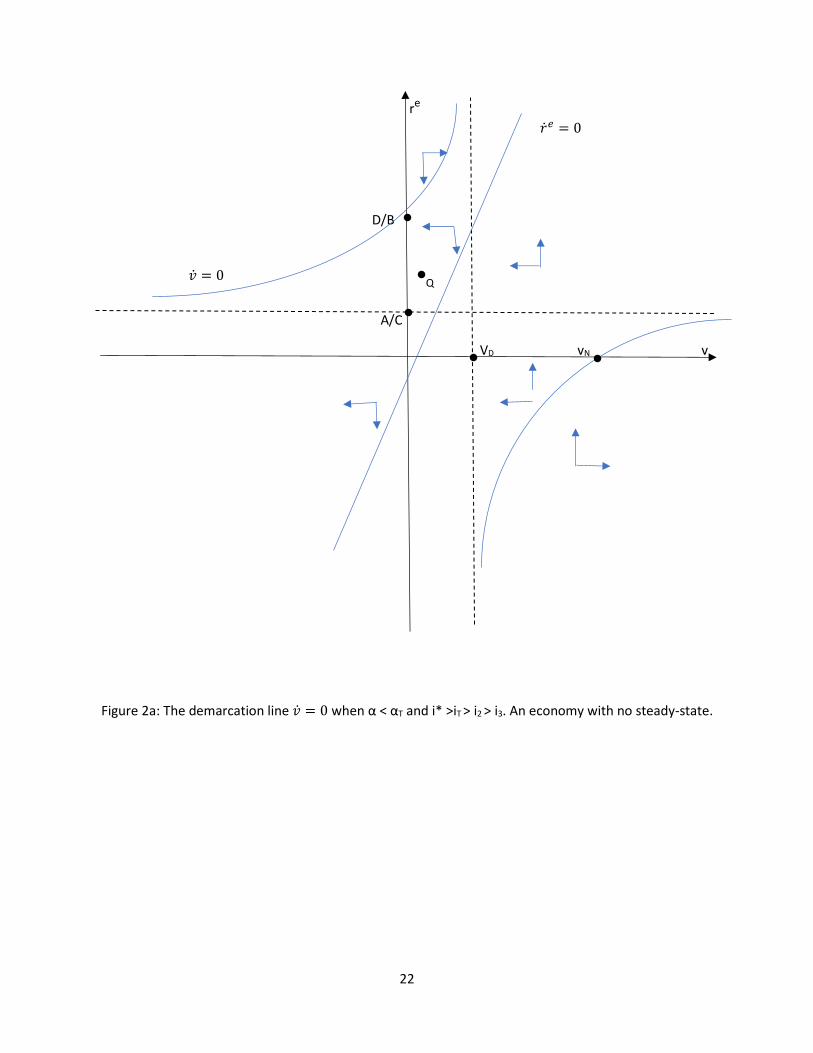
Figure 2a: The demarcation line �̇� = 0 when α < αT and i* >iT > i2 > i3. An economy with no steady-state.
�̇� = 0
�̇�𝑒 = 0

23
re
S
U
vD v
Figure 2b: The demarcation line �̇� = 0 when α < αT and i* >iT > i2 > i3. An economy with a steady-state.
�̇�𝑒 = 0
�̇� = 0
= 0

24
re
A/C
Q
D/B P
vN vD v
Figure 3: The demarcation line �̇� = 0 when α < αT and iT > i* > i2 > i3.
�̇�𝑒 = 0
�̇� = 0
S
25
re
A/C
P
vN vD v
D/B
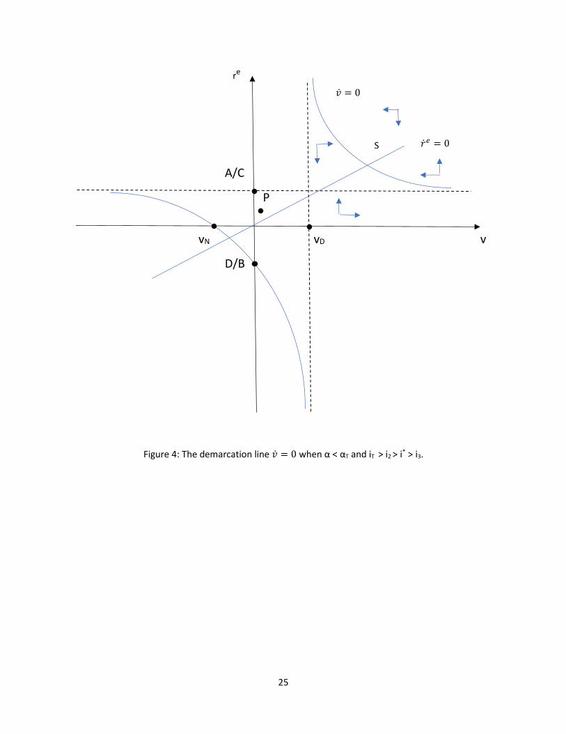
Figure 4: The demarcation line �̇� = 0 when α < αT and iT > i2 > i* > i3.
�̇�𝑒 = 0 S
�̇� = 0

26
re
vD vN
v
A/C
D/B
Figure 5a: The demarcation line �̇� = 0 when α < αT and iT > i2 > i3 > i*. A positive profit rate.
�̇�𝑒 = 0 S
�̇� = 0

27
re
vD vN
v
T
A/C
Figure 5b: the demarcation line �̇� = 0 when α < αT and iT > i2 > i3 > i*. A negative profit rate.
Figures from 2 to 5 illustrate the inter-temporal behavior of an economy characterized by a weak
preference for cash (α ‹ αT). The small horizontal arrows in the different diagrams are intended
to show that, as proved in the Appendix, the only branch of the rectangular hyperbola attracting
the economy when it stays outside the isocline �̇� = 0 is that lying above its horizontal asymptote.
The different subcases are associated to different levels of the world interest rate, i*: moving
from figure 2 to figure 5, the world interest rate goes down, everything else remaining
unchanged.
An intertemporal equilibrium (steady state) for this economy is a point of intersection between
the isoclines �̇�𝑒 = 0 (the straight line) and �̇� = 0 (the rectangular hyperbola). A simple visual

28
inspection of our diagrams should persuade the reader that whereas in the sub-cases illustrated
in figures 3, 4 and 5, a locally stable steady-state certainly exists (simply because the slope of
�̇�𝑒 = 0 is always positive and finite and then, sooner or later, this isocline must intersect with the
stable branch of �̇� = 0), this is not necessarily true when the interest rate is very high. This is the
unpleasant case illustrated in figure 2, where
𝑖∗ > 𝑖𝑇 =𝑏0(1−𝑐1+𝑏2)−𝑏2𝑐2
(1+𝑏2)[𝑏2+𝛼(1−𝑐1)] (15)
The world interest rate is above the threshold defined by (15) and fully derived in the Appendix,
and a stable steady state might not exist. This possibility of non-existence is represented in figure
2a, where the two isoclines do not intersect. The economy we are talking about is indebted
toward the RoW16 and the world interest rate is simply too high. Even if people have a weak
preference for cash (which in itself slows the accumulation of foreign debt), the economy cannot
sustain such a high interest rate and falls endlessly into the hell, i.e. the region with negative
wealth, negative profit rates and negative capital accumulation.
It must be noted, however, that the economy we are talking about - a regime of weak preference
for cash and 𝑖∗ > 𝑖𝑇 – might end up in a locally stable steady state and, at least in principle, the
case illustrated in figure 2a is not an inevitable destiny. Start from figure 2a, and imagine that
income distribution worsens, i.e. the profit share (1 – ψ) goes up. The isocline �̇�𝑒 = 0 becomes
steeper, whereas the rectangular hyperbola remains unaffected. The final outcome could be that
illustrated in figure 2b, where the economy reaches the stable steady-state S (U is an unstable
steady-state, a saddle point)17. However, which kind of economy is represented in figure 2b? Do
not forget that S is a locally stable steady state, which means that the economy will actually reach
that point only starting from a “sufficiently small” neighborhood. So, the economy we are talking
about is one which is indebted toward the rest of the world and that, despite having to pay a very
high interest rate to foreign creditors, is able to reach a steady state characterized by a relatively
high profit rate. This may only happen (look at (4)) when income distribution is tremendously
16 Observe that along the stable branch of the rectangular hyperbola it is always v < vD < 1 < 1/(1 – α), vD being defined in the Appendix. 17 Needless to say, the growth of the profit share does not have to violate (12), otherwise internal instability would just replace external instability.

29
skewed in favor of industrialists and against workers: an otherwise financially unsustainable
scenario becomes sustainable in that workers accept to remain silent18. If this is not the case and
such an awful steady state is not achieved because of some kind of real wage resistance, we are
back to figure 2a, to the case of an economy that, once reached the isocline �̇�𝑒 = 0 (an attractor),
goes towards minus infinity: even if the preference for cash is weak, the interest rate is so high
that sooner or later the process of accumulation ceases and foreign debt becomes unsustainable.
In sum, the case of a very high interest rate represented in figures 2a and 2b gives people very
few options. Either they accept the Scylla of a socially awful equilibrium or they go for the
Charybdis of a financial disaster (from the perspective of workers the difference, if any, is
probably irrelevant).
Admittedly, the case illustrated in figure 2 is unlikely, it needs a very high world interest rate to
materialize. Luckily enough, things are different when the world interest rate lowers. Take figure
3. Though higher, the intercept on the vertical axis of the isocline �̇�𝑒 = 0 is again negative. There
are two steady states, but only S is (locally) stable (the other is, again, a saddle point). The big
difference with the scenario depicted in figure 2 is that in this case a locally stable steady state
certainly exists. Of course, it is still possible for the economy, even in this “improved” scenario,
to go towards minus infinity (foreign debt becomes unsustainable and stops accumulation). This
is for instance the case of an economy starting from very low (however positive) levels of both
the expected profit rate and the wealth-to-capital ratio, in a point like P somewhat close to the
origin (and below the unstable branch of the hyperbola). There is little doubt, however, that this
miserable outcome is less likely than it was in the previous case, characterized by a higher world
interest rate (figure 2): even when the starting levels of re and v are relatively low - in a point like
Q, for instance (lying this time above the unstable branch of the hyperbola), a point that would
push the economy towards minus infinity in the case of figure 2 - the economy might well end up
in the steady-state S, especially when profit expectations do not adjust too rapidly. Observe,
moreover, that in the steady state S the economy might result to be net creditor towards the rest
18 In a model where income distribution affects aggregate demand and output and growth happen to be “wage-led” (Bhaduri and Marglin, 1990), not even workers’ silence would be enough.

30
of the world. Of course, this is not to be taken for granted19, but as we saw this possibility was
just to be ruled out in the case illustrated by figure 2.
Things are even better in figure 4, with a still lower world interest rate. In this case we cannot say
whether the intercept on the vertical axis of the isocline �̇�𝑒 = 0 is positive or negative20, but this
is not important to know. In any case, indeed, the economy is very likely to reach a stable steady-
state like S, with positive v and r. Observe, in particular, that even in case the economy starts
from a point like P – a point that would have pushed the system towards minus infinity in the
case illustrated by figure 3 – it will end up in the steady-state S.
As to figure 5 – the lowest world interest rate in a regime of weak preference for cash – we can
observe that, once again, we are not sure that the intercept on the vertical axis of the isocline
�̇�𝑒 = 0 becomes positive21. In case it is positive (figure 5a: preference for cash is extremely low,
see footnote 17), the economy reaches a stable steady state like S almost from everywhere. In
case it is negative (figure 5b: preference for cash is not as low as it is in figure 5a), the economy
could in principle end up in a stable steady state like T, with a negative profit rate. Again, which
kind of economy we are talking about? How is it possible to have a negative profit rate with such
a low interest rate? Even if this is not to be taken for granted, the economy we are dealing with
is likely to be a net creditor in international financial markets22 (or, at worst, a “weak” debtor). In
this case, the profit rate might well lower with falling interest rates, especially when the wage
share is high (as it can be easily seen from the short-run solution of the model). Needless to say,
the case illustrated by figure 5b is extremely unlikely to materialize. It is more a theoretical
19 Observe that, in S, v > vD, but we do not whether v > 1/(1 – α). This depends (and obviously so) on several other parameters of the economy. 20 The argument goes as follows. To be sure that the intercept continues to be negative, we should be able to say that i* > i1, but we only know that i* > i3. This would be enough when i3 > i1 but, as proved in the Appendix, for this to be true it must be α > αH, with αH < αT. Well, we just know that, in the case illustrated by Figure 4, α < αT and therefore we cannot conclude. 21 The argument is essentially the same we developed in footnote 16. To be sure that the intercept becomes positive, we need α < αH, but we only know that α < αT, and αH < αT. 22 Observe, indeed, that in the steady-state T we have v > vN > vD. In words, the wealth-to-capital ratio is very high, as it is the case for a creditor economy. That said, we cannot take it for granted that the economy at hand is a net creditor, since v > vN certainly implies v > 1/(1 – α) only when α > αT (i.e. in a regime of strong preference for cash), as the reader can easily prove by using the definition of vN given in the Appendix.
31
curiosum than a concrete possibility, especially because it is very hard to think of a steady state
with negative profit rates23.
4.4.2 Strong preference for cash
Let us move now to the regime of a strong preference for cash, α › αT.
re
D/B
A/C
vD vN v
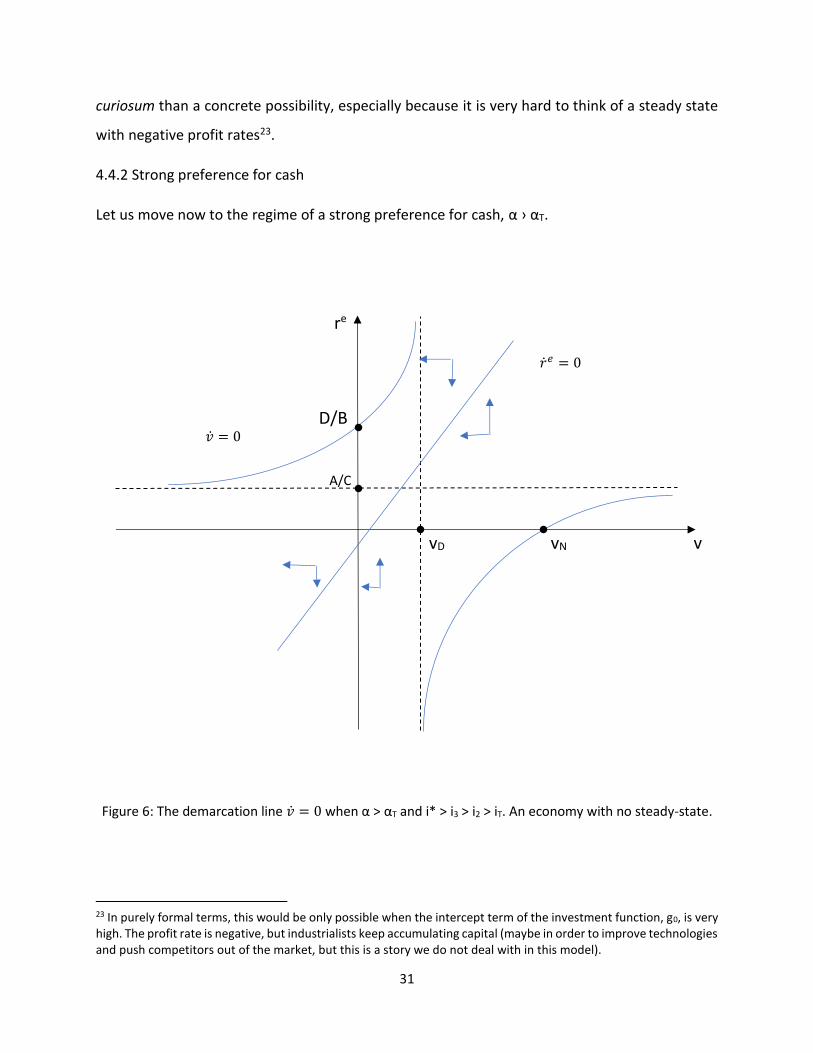
Figure 6: The demarcation line �̇� = 0 when α > αT and i* > i3 > i2 > iT. An economy with no steady-state.
23 In purely formal terms, this would be only possible when the intercept term of the investment function, g0, is very high. The profit rate is negative, but industrialists keep accumulating capital (maybe in order to improve technologies and push competitors out of the market, but this is a story we do not deal with in this model).
�̇�𝑒 = 0
�̇� = 0

32
re
D/B
vN vD
v
A/C
Figure 7: The demarcation line �̇� = 0 when α > αT and iT < i2 < i* < i3. Once again there is no steady-state
�̇�𝑒 = 0
�̇� = 0

33
re
vN vD
D/B v
A/C
Figure 8: α > αT, i3 > i2 > i* > iT
�̇�𝑒 = 0

34
re
S’
vD vN v
A/C
D/B
Figure 9: α > αT, i3 > i2 > iT > i*
Again, an overall visual inspection of figures from 6 to 9, with the world interest rate falling from
high to low levels, is useful. It immediately makes it clear that, apart from the case of figure 9 (of
a very low world interest rate), the position of our rectangular hyperbola is such that the two
isoclines might not intersect. In a regime of weak preference for cash, this possibility was only
there for a very high world interest rate (figure 2). Here, on the contrary, it applies to a wider
range of interest rates. The economic rationale is simple. A higher preference for cash, as such,
accelerates the accumulation of foreign debt and therefore, even with not too high world interest
rates, the risk of falling into a debt trap increases.
�̇�𝑒 = 0
35
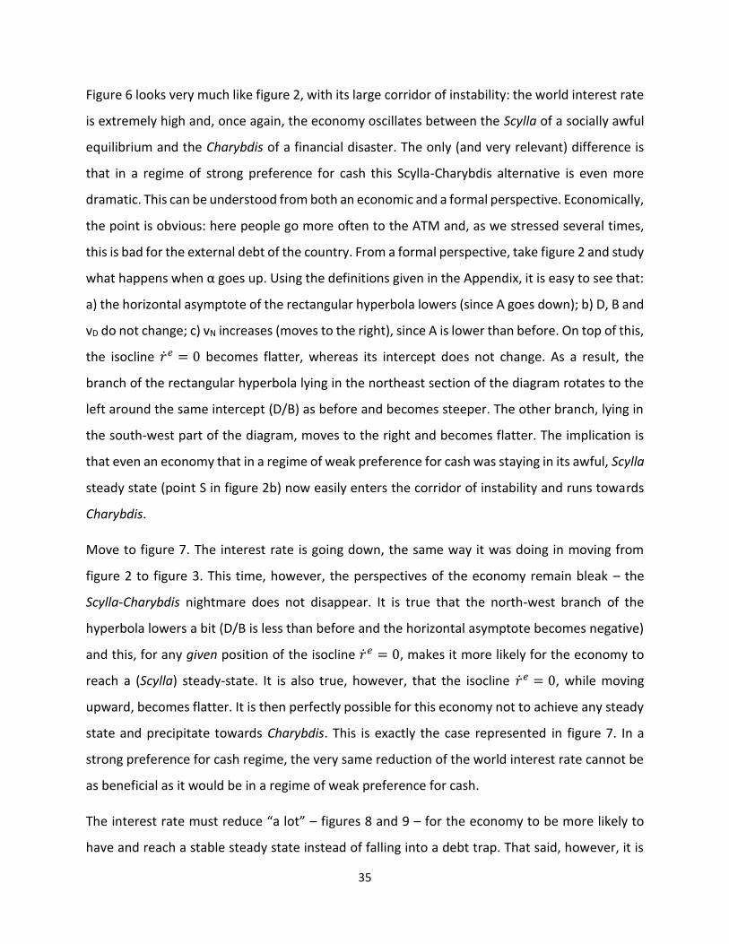
Figure 6 looks very much like figure 2, with its large corridor of instability: the world interest rate
is extremely high and, once again, the economy oscillates between the Scylla of a socially awful
equilibrium and the Charybdis of a financial disaster. The only (and very relevant) difference is
that in a regime of strong preference for cash this Scylla-Charybdis alternative is even more
dramatic. This can be understood from both an economic and a formal perspective. Economically,
the point is obvious: here people go more often to the ATM and, as we stressed several times,
this is bad for the external debt of the country. From a formal perspective, take figure 2 and study
what happens when α goes up. Using the definitions given in the Appendix, it is easy to see that:
a) the horizontal asymptote of the rectangular hyperbola lowers (since A goes down); b) D, B and
vD do not change; c) vN increases (moves to the right), since A is lower than before. On top of this,
the isocline �̇�𝑒 = 0 becomes flatter, whereas its intercept does not change. As a result, the
branch of the rectangular hyperbola lying in the northeast section of the diagram rotates to the
left around the same intercept (D/B) as before and becomes steeper. The other branch, lying in
the south-west part of the diagram, moves to the right and becomes flatter. The implication is
that even an economy that in a regime of weak preference for cash was staying in its awful, Scylla
steady state (point S in figure 2b) now easily enters the corridor of instability and runs towards
Charybdis.
Move to figure 7. The interest rate is going down, the same way it was doing in moving from
figure 2 to figure 3. This time, however, the perspectives of the economy remain bleak – the
Scylla-Charybdis nightmare does not disappear. It is true that the north-west branch of the
hyperbola lowers a bit (D/B is less than before and the horizontal asymptote becomes negative)
and this, for any given position of the isocline �̇�𝑒 = 0, makes it more likely for the economy to
reach a (Scylla) steady-state. It is also true, however, that the isocline �̇�𝑒 = 0, while moving
upward, becomes flatter. It is then perfectly possible for this economy not to achieve any steady
state and precipitate towards Charybdis. This is exactly the case represented in figure 7. In a
strong preference for cash regime, the very same reduction of the world interest rate cannot be
as beneficial as it would be in a regime of weak preference for cash.
The interest rate must reduce “a lot” – figures 8 and 9 – for the economy to be more likely to
have and reach a stable steady state instead of falling into a debt trap. That said, however, it is
36
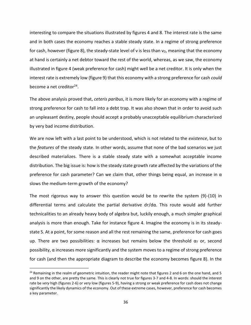
interesting to compare the situations illustrated by figures 4 and 8. The interest rate is the same
and in both cases the economy reaches a stable steady state. In a regime of strong preference
for cash, however (figure 8), the steady-state level of v is less than vD, meaning that the economy
at hand is certainly a net debtor toward the rest of the world, whereas, as we saw, the economy
illustrated in figure 4 (weak preference for cash) might well be a net creditor. It is only when the
interest rate is extremely low (figure 9) that this economy with a strong preference for cash could
become a net creditor24.
The above analysis proved that, ceteris paribus, it is more likely for an economy with a regime of
strong preference for cash to fall into a debt trap. It was also shown that in order to avoid such
an unpleasant destiny, people should accept a probably unacceptable equilibrium characterized
by very bad income distribution.
We are now left with a last point to be understood, which is not related to the existence, but to
the features of the steady state. In other words, assume that none of the bad scenarios we just
described materializes. There is a stable steady state with a somewhat acceptable income
distribution. The big issue is: how is the steady state growth rate affected by the variations of the
preference for cash parameter? Can we claim that, other things being equal, an increase in α
slows the medium-term growth of the economy?
The most rigorous way to answer this question would be to rewrite the system (9)-(10) in
differential terms and calculate the partial derivative dr/dα. This route would add further
technicalities to an already heavy body of algebra but, luckily enough, a much simpler graphical
analysis is more than enough. Take for instance figure 4. Imagine the economy is in its steady-
state S. At a point, for some reason and all the rest remaining the same, preference for cash goes
up. There are two possibilities: α increases but remains below the threshold αT or, second
possibility, α increases more significantly and the system moves to a regime of strong preference
for cash (and then the appropriate diagram to describe the economy becomes figure 8). In the
24 Remaining in the realm of geometric intuition, the reader might note that figures 2 and 6 on the one hand, and 5 and 9 on the other, are pretty the same. This is clearly not true for figures 3-7 and 4-8. In words: should the interest rate be very high (figures 2-6) or very low (figures 5-9), having a strong or weak preference for cash does not change significantly the likely dynamics of the economy. Out of these extreme cases, however, preference for cash becomes a key parameter.

37
first case – look at figure 10 for an illustration – the isocline �̇�𝑒 = 0 becomes flatter and the stable
branch of the isocline �̇� = 0 shifts downward (vD does not change, whereas A/C lowers and this
shifts the horizontal asymptote down). Therefore, we do not know a priori whether the steady-
state level of the wealth-to-capital ratio goes up or down (in figure 10 it goes up, but this is only
a possibility25), but it is certainly true that dr/dα < 0. There are no ambiguities at all: a stronger
preference for cash reduces the steady state profit rate and then, just look at (3), the steady state
growth rate of the economy.
r
S
A/C
A’/C S’
VD V
Figure 10: the impact of a higher α on profits and growth
25 The ambiguous effect on the wealth-to-capital ratio results from the existence of two different forces at work. On the one hand, there is a direct and negative effect on foreign debt: banks borrow more from abroad to satisfy households’ extra-demand for cash. On the other hand, there is an indirect and positive effect on the accumulation of foreign debt: capital accumulation is now slower, and banks borrow less from abroad because they are lending less to domestic firms.
38
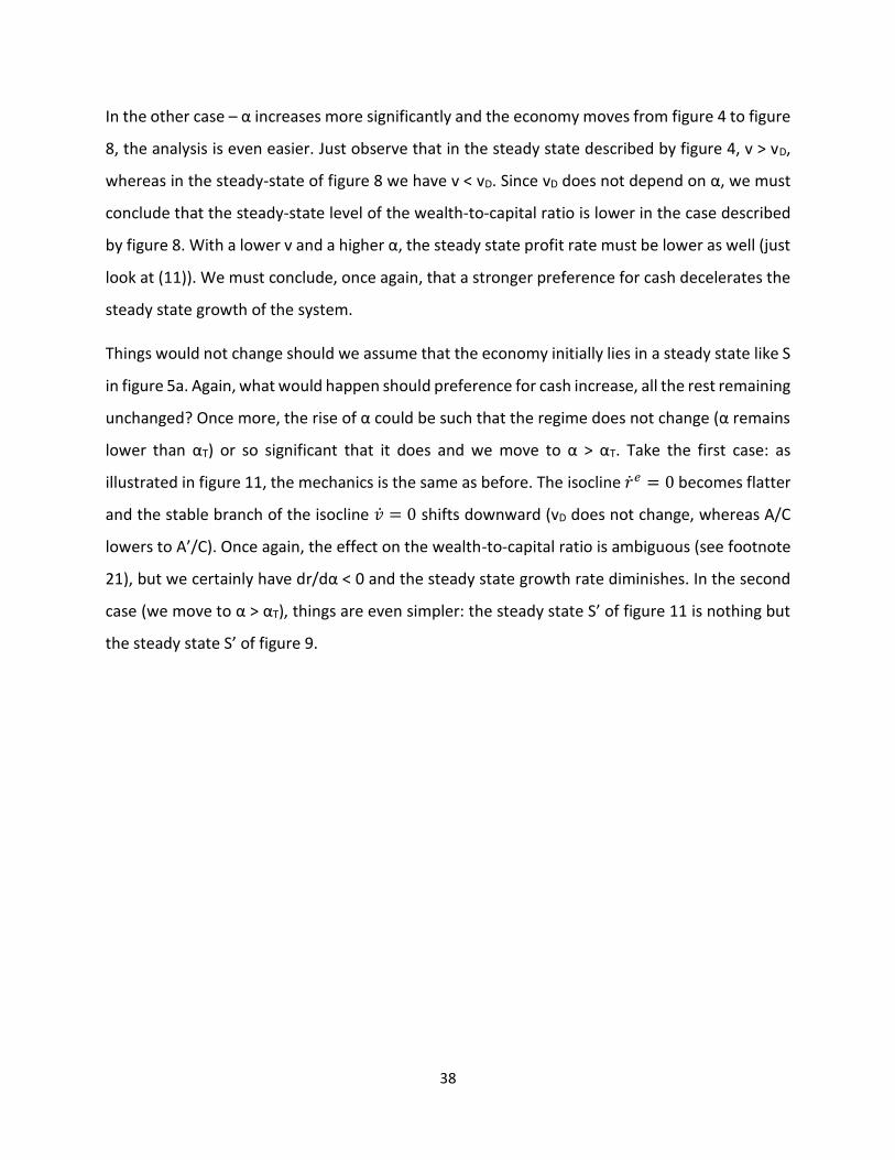
In the other case – α increases more significantly and the economy moves from figure 4 to figure
8, the analysis is even easier. Just observe that in the steady state described by figure 4, v > vD,
whereas in the steady-state of figure 8 we have v < vD. Since vD does not depend on α, we must
conclude that the steady-state level of the wealth-to-capital ratio is lower in the case described
by figure 8. With a lower v and a higher α, the steady state profit rate must be lower as well (just
look at (11)). We must conclude, once again, that a stronger preference for cash decelerates the
steady state growth of the system.
Things would not change should we assume that the economy initially lies in a steady state like S
in figure 5a. Again, what would happen should preference for cash increase, all the rest remaining
unchanged? Once more, the rise of α could be such that the regime does not change (α remains
lower than αT) or so significant that it does and we move to α > αT. Take the first case: as
illustrated in figure 11, the mechanics is the same as before. The isocline �̇�𝑒 = 0 becomes flatter
and the stable branch of the isocline �̇� = 0 shifts downward (vD does not change, whereas A/C
lowers to A’/C). Once again, the effect on the wealth-to-capital ratio is ambiguous (see footnote
21), but we certainly have dr/dα < 0 and the steady state growth rate diminishes. In the second
case (we move to α > αT), things are even simpler: the steady state S’ of figure 11 is nothing but
the steady state S’ of figure 9.

39
r
S
S’
V
A/C
A’/C
Figure 11: the impact of a higher α on profits and growth
5. Conclusions and extensions
In a world of endogenous money, where commercial banks may and do create money by making
loans and make loans each time this is perceived as profitable, what are the consequences of
being “dollarized”, i.e. not having the right to print an own currency? Of course, should people
not be interested in holding cash as a store of value and be content with their bank deposits,
nothing relevant would change. You would not have the right to print pieces of paper people do
not want to hold.
However, as argued in the paper, in dollarized economies people preference for cash (i.e. the
desire of people to hold cash as a store of value), is inevitably higher than in countries with their
own currencies. A dollarized economy is much more likely to live in a regime of strong preference
40
for cash compared to an economy with its own currency. In the paper, we have shown that it is
more likely for an economy with a strong preference for cash (a dollarized economy) to fall into
a debt trap. It was also shown that in order to avoid such an unpleasant destiny, an economy
with a strong preference for cash should accept a probably unacceptable equilibrium with a very
bad income distribution. Last but not least, it was also shown that when a dollarized economy
reaches a stable steady state, this (everything being equal) is characterized by a lower growth
rate compared to that of an economy with its own currency.
These are important results. They suggest that once dollarization has done its job and inflation is
back to some acceptable level, countries should try to return to their own currency. That said, a
couple of further observations are to be proposed. First, there might be cases – think of Panama
– where dollarization is not as costly as depicted in this paper. The reason is simple: the political
link between Panama and the USA is much stronger and more solid than, say, that between
Ecuador and the USA. This means that people in Panama, differently from people in Ecuador, do
not have strong reasons to believe that, in case of need, the extra-demand for cash will not be
satisfied by printing more of it. The FED will just do it. In terms of the model proposed in the
paper, the parameter α in Panama is likely to be the same it is in any other monetarily sovereign
country (and a very low parameter, of course), but this is certainly not the case in Ecuador. The
second observation refers to a possible extension of this model. If remaining dollarized so long is
so costly, why is it that “de-dollarization” does not happen more often and more rapidly? The
model proposed in this paper is too aggregate to offer some possible answer. It is just unable to
identify those concrete forces working in the social fabric against de-dollarization. An extended
model should then explicitly include a class analysis and, in particular, the possibility for the
richest segment of the population to hold securities issued abroad (the so-called “capital flights”).

41
Appendix
The derivation of equation (9)
Equation (1bis) implies
�̇� = −1
1−𝛼𝑙�̇� (A1)
Of course, the stationarity of the external debt-to-capital ratio implies that of the wealth-to-
capital ratio (and vice versa), and we can study the evolution of the former to understand the
dynamics of the latter. From the definition lf = qLf/K and remembering that q = 1/P is taken as
given (�̂� = 0) we get (as usual, a “hat” over a variable denotes its growth rate)
𝑙𝑓 = �̂�𝑓 − 𝑔 (A2)
Using national accounts (the flows-of-funds in table FM are enough), one gets
�̇�𝑓 = �̇� − 𝑁𝐹𝐴 =̇ �̇� − 𝑁𝐶𝐴 (A3)
However simple, the notion incorporated in equation (A3) is key. Even if the net foreign asset
position does not change (the nominal current account NCA is zero), in a dollarized economy
foreign debt increases to the extent that people want to hold more cash as a store of value (�̇� >
0).
Dividing by the stock of foreign debt and normalizing by the capital stock, (A3) becomes
�̂�𝑓 =�̇�
𝑃𝐾−𝑐𝑎
𝑙𝑓 (A4)
Let us insert (A4) into (A2):
𝑙�̇� =�̇�
𝑃𝐾− 𝑐𝑎 − 𝑔𝑙𝑓 (A5)
Now, using our assumption that people keep a fraction α of their wealth in the form of cash (H =
αV), (A5) may be written as

42
𝑙�̇� = 𝛼�̇�
𝑃𝐾− 𝑐𝑎 − 𝑔𝑙𝑓 (A6)
By the definition of v we get
�̇�
𝑃𝐾= �̇� + 𝑣𝑔
Hence,
𝑙�̇� = 𝛼(�̇� + 𝑣𝑔) − 𝑐𝑎 − 𝑔𝑙𝑓 (A7).
This is not yet the end of the story. Using (1bis), (A7) may be written as
𝑙�̇� = 𝛼 (�̇� +1−𝑙𝑓
1−𝛼𝑔) − 𝑐𝑎 − 𝑔𝑙𝑓
Rearranging:
𝑙�̇� = 𝛼�̇� − 𝑐𝑎 + 𝑔(𝛼−𝑙𝑓)
(1−𝛼) (A8)
Now drop (A8) into (A1). Using (1bis), one gets exactly the differential equation (9) of the text;
�̇� = 𝑐𝑎 + 𝑔(1 − 𝑣)
The demarcation line �̇� = 0
The equation of the demarcation line �̇� = 0 (equation (14) in the text), i.e.
{𝑖∗(1 − 𝛼)(1 − 𝑐1)(1 + 𝑏2) − 𝑏2𝑐2 − 𝑔0(1 − 𝑐1 + 𝑏2)}𝑣 + [(1 − 𝑐1)𝑔1]𝑟𝑒 − [(1 − 𝑐1 + 𝑏2)𝑔1]𝑣𝑟𝑒 =
(1 − 𝑐1)[𝑖∗(1 + 𝑏2) − 𝑏0 − 𝑔0]
may be written as
𝐴𝑣 + 𝐵𝑟𝑒 − 𝐶𝑣𝑟𝑒 = 𝐷,
having defined the parameters
𝐴 = {𝑖∗(1 − 𝛼)(1 − 𝑐1)(1 + 𝑏2) − 𝑏2𝑐2 − 𝑔0(1 − 𝑐1 + 𝑏2)}
𝐵 = [(1 − 𝑐1)𝑔1]

43
𝐶 = [(1 − 𝑐1 + 𝑏2)𝑔1]
𝐷 = (1 − 𝑐1)[𝑖∗(1 + 𝑏2) − 𝑏0 − 𝑔0] .
Its solution is
𝑟𝑒 =𝐷−𝐴𝑣
𝐵−𝐶𝑣 (A9),
which is the equation of a rectangular hyperbola. We know that B > 0 and C > 0, but the signs of
A and D are ambiguous. They are to be studied carefully to draw our rectangular hyperbola. First,
𝐷 ⋛ 0 ⇔ 𝑖∗ ⋛(𝑏0+𝑔0)
(1+𝑏2)= 𝑖2 > 0
Notice that short-run stability (1 − 𝑐1 + 𝑏2 > 0) is enough to guarantee that i2 > i1, the latter
being defined by (13) in the text. As to A,
𝐴 ⋛ 0 ⇔ 𝑖∗ ⋛𝑏2𝑐2+𝑔0
(1−𝑐1+𝑏2)
(1−𝛼)(1−𝑐1)(1+𝑏2)= 𝑖3 > 0
Observe that
𝑖3 ⋛ 𝑖2 ⇔ 𝛼 ⋛ 𝛼𝑇 =𝑏0(1−𝑐1)−𝑏2(𝑔0+𝑐2)
𝑏0(1−𝑐1)+𝑔0(1−𝑐1).
So, using the definitions of the text, 𝑖3 > 𝑖2 in a regime of “strong” preference for cash, whereas
𝑖3 < 𝑖2 in a regime of “weak preference for cash”.
In some cases, it might be useful to understand the relation between i1 and i3. Well, it is easy to
show that
𝑖1 > 𝑖3 ⇔ 𝛼 < 𝛼𝐻 =𝑏0(1−𝑐1)(1+𝑏2)(1−𝜓)−𝑏2(𝑔0+𝑐2)(1+𝑏2−𝜓𝑐1)−𝜓𝑔0(1−𝑐1)(1−𝑐1+𝑏2)
𝑏0(1−𝑐1)(1+𝑏2)(1−𝜓)+𝑔0(1−𝑐1)(1+𝑏2)(1−𝜓)
Clearly, 𝛼𝐻 < 1 under any possible parametric configuration. Moreover, one can easily check
that 𝛼𝑇 > 𝛼𝐻.
Of course, (A9) is not defined for B = Cv, i.e. for
𝑣 =𝐵
𝐶=
(1−𝑐1)
(1−𝑐1+𝑏2)= 𝑣𝐷

44
The parameter 𝑣𝐷, with 0 < 𝑣𝐷 < 1, defines the vertical asymptote of our rectangular hyperbola.
Note, also, that when 𝑣 < 𝑣𝐷 (𝑣 > 𝑣𝐷), the denominator of (A9) is positive (negative). As to the
numerator, D – Av, one should pay attention and note that
𝐼𝑓 𝐴 > 0 (𝑖∗ > 𝑖3) ⇒ 𝐷 − 𝐴𝑣 > 0 ⇔ 𝑣 <𝐷
𝐴
𝐼𝑓 𝐴 < 0 (𝑖∗ < 𝑖3) ⇒ 𝐷 − 𝐴𝑣 > 0 ⇔ 𝑣 >𝐷
𝐴
For future reference, it is convenient to define the parameter
𝑣𝑁 =𝐷
𝐴=
(1−𝑐1)[𝑖∗(1+𝑏2)−𝑏0−𝑔0]
{𝑖∗(1−𝛼)(1−𝑐1)(1+𝑏2)−𝑏2𝑐2−𝑔0(1−𝑐1+𝑏2)}
Note, also, that the function (A9) passes through the point (vN, 0). It is important to establish the
relation between 𝑣𝐷 and 𝑣𝑁. Four possibilities may arise:
𝐼𝑓 𝐷 > 0 (𝑖∗ > 𝑖2) 𝑎𝑛𝑑 𝐴 > 0 (𝑖∗ > 𝑖3) ⇒ 𝑣𝐷 > 𝑣𝑁 ⇔ 𝐴𝐵 > 𝐷𝐶 ⇔ 𝑖∗ < 𝑖𝑇 =
𝑏0(1−𝑐1+𝑏2)−𝑏2𝑐2
(1+𝑏2)[𝑏2+𝛼(1−𝑐1)]
𝐼𝑓 𝐷 < 0 (𝑖∗ < 𝑖2) 𝑎𝑛𝑑 𝐴 < 0 (𝑖∗ < 𝑖3) ⇒ 𝑣𝐷 > 𝑣𝑁 ⇔ 𝐴𝐵 < 𝐷𝐶 ⇔ 𝑖∗ > 𝑖𝑇 =
𝑏0(1−𝑐1+𝑏2)−𝑏2𝑐2
(1+𝑏2)[𝑏2+𝛼(1−𝑐1)]
𝐼𝑓 𝐷 < 0 (𝑖∗ < 𝑖2) 𝑎𝑛𝑑 𝐴 > 0 (𝑖∗ > 𝑖3) ⇒ 𝑣𝐷 > 𝑣𝑁 ⇔ 𝐴𝐵 > 𝐷𝐶 𝑎𝑙𝑤𝑎𝑦𝑠 𝑡𝑟𝑢𝑒
𝐼𝑓 𝐷 > 0 (𝑖∗ > 𝑖2) 𝑎𝑛𝑑 𝐴 < 0 (𝑖∗ < 𝑖3) ⇒ 𝑣𝐷 > 𝑣𝑁 ⇔ 𝐴𝐵 < 𝐷𝐶 𝑎𝑙𝑤𝑎𝑦𝑠 𝑡𝑟𝑢𝑒
It is now time to investigate the relation between iT, i2 and i3. First, simple calculations show that
𝑖𝑇 > 𝑖2 ⇔ 𝛼 < 𝛼𝑇
(note, also, that 𝛼𝑇 > 0 ⇒ 𝑖𝑇 > 0). As to the relation between iT and i3, the turning value is once
again 𝛼𝑇:
𝑖𝑇 > 𝑖3 ⇔ 𝛼 < 𝛼𝑇
From (A1), one can see that the first and second derivative of the isocline are
𝜕𝑟𝑒
𝜕𝑣=
𝐷𝐶−𝐴𝐵
(𝐵−𝐶𝑣)2
45
and
𝜕2𝑟𝑒
(𝜕𝑣)2=
2(𝐷𝐶−𝐴𝐵)
(𝐵−𝐶𝑣)3 .
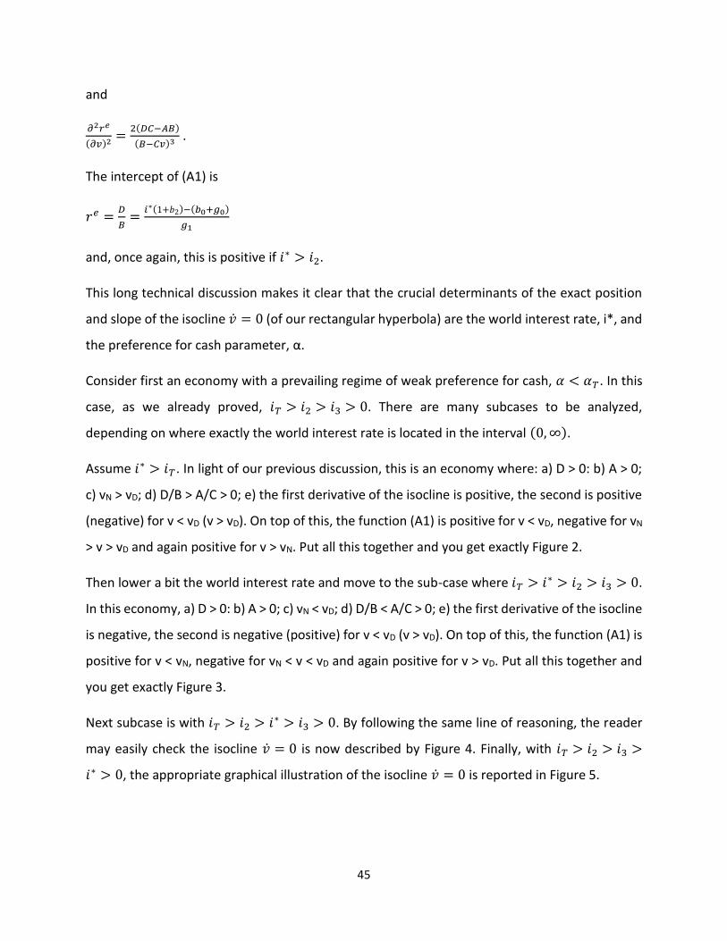
The intercept of (A1) is
𝑟𝑒 =𝐷
𝐵=
𝑖∗(1+𝑏2)−(𝑏0+𝑔0)
𝑔1
and, once again, this is positive if 𝑖∗ > 𝑖2.
This long technical discussion makes it clear that the crucial determinants of the exact position
and slope of the isocline �̇� = 0 (of our rectangular hyperbola) are the world interest rate, i*, and
the preference for cash parameter, α.
Consider first an economy with a prevailing regime of weak preference for cash, 𝛼 < 𝛼𝑇. In this
case, as we already proved, 𝑖𝑇 > 𝑖2 > 𝑖3 > 0. There are many subcases to be analyzed,
depending on where exactly the world interest rate is located in the interval (0, ∞).
Assume 𝑖∗ > 𝑖𝑇. In light of our previous discussion, this is an economy where: a) D > 0: b) A > 0;
c) vN > vD; d) D/B > A/C > 0; e) the first derivative of the isocline is positive, the second is positive
(negative) for v < vD (v > vD). On top of this, the function (A1) is positive for v < vD, negative for vN
> v > vD and again positive for v > vN. Put all this together and you get exactly Figure 2.
Then lower a bit the world interest rate and move to the sub-case where 𝑖𝑇 > 𝑖∗ > 𝑖2 > 𝑖3 > 0.
In this economy, a) D > 0: b) A > 0; c) vN < vD; d) D/B < A/C > 0; e) the first derivative of the isocline
is negative, the second is negative (positive) for v < vD (v > vD). On top of this, the function (A1) is
positive for v < vN, negative for vN < v < vD and again positive for v > vD. Put all this together and
you get exactly Figure 3.
Next subcase is with 𝑖𝑇 > 𝑖2 > 𝑖∗ > 𝑖3 > 0. By following the same line of reasoning, the reader
may easily check the isocline �̇� = 0 is now described by Figure 4. Finally, with 𝑖𝑇 > 𝑖2 > 𝑖3 >
𝑖∗ > 0, the appropriate graphical illustration of the isocline �̇� = 0 is reported in Figure 5.

46
Let us move now to a regime of strong preference for cash, i.e. 𝛼 > 𝛼𝑇. In this case, 𝑖𝑇 < 𝑖2 < 𝑖3.
Once again, there are four subcases and, using the same argument as before (lowering the world
interest rate), the reader may easily check that they give rise to figures from 6 to 9.
What happens when the economy lies outside the isocline �̇� = 0? Note that
𝜕�̇�
𝜕𝑟𝑒 = 𝑔1[(1 − 𝑐1) − (1 − 𝑐1 + 𝑏2)] ⋛ 0 ⇔ 𝑣 ⋚ 𝑣𝐷,
implying that the only branch of the rectangular hyperbola that attracts the economy is that
located above the horizontal asymptote (regardless of whether the latter is positive or negative),
as indicated by the small arrows in our diagrams.

47
References
Acosta, A. and J. Cajas Guijarro (2018), Una década desperdiciada. Las sombras del correismo,
Centro Andino de Accion Popular, Quito.
Bhaduri, A. And S. Marglin (1990), Unemployment and the Real Wage: the economic basis for
contesting political ideologies, Cambridge Journal of Economics, volume 4, Issue 4, 375-393.
Correa, R. (2019), La fabrique de la politique économique équatorienne. Le point de vue d’un
acteur clé, interview, Revue de la Régulation, 25(1).
Dullien, S. (2009), Central banking, Financial Institutions and Credit Creation in Developing
Countries, UNCTAD Discussion Papers, No. 193.
Izurieta, A. (2003), Dollarization as a tight rein on the fiscal stance, in Rochon, L.P. and M.
Seccareccia (eds.) (2003), Dollarization. Lessons from Europe and the Americas, Routledge,
London and New York.
Paredes, G.J. (2017), Ecuador: why exit dollarization?, CEPAL Review no. 121
Ponsot, J.F. (2019), Economie Politique de la dollarisation, in Mondes en Développement, Vol. 47-
2019/4-n.188
Rochon, L.P. and M. Seccareccia (eds.) (2003), Dollarization. Lessons from Europe and the
Americas, Routledge, London and New York.
Rowthorn, R.E. (1977), Conflict, Inflation and Money, Cambridge Journal of Economics, volume 1,
Issue 3, 215-39.
Taylor, L. and P. Krugman (1978), Contractionary Effects of Devaluations, Journal of International
Economics, volume 8, issue 3, 445-456
Taylor, L. (1983), Structuralist Macroeconomics, Basic Books
Thirlwall, A. P. (1997), Reflection on the Concept of Balance-of-Payments-Constrained Growth,
Journal of Post-Keynesian Economics, Volume 19, Issue 3.
Weintraub, S. (1958), An Approach to the Theory of Income Distribution, Philadelphia: Chilton.

48
World Bank (2008), West Bank and Gaza. Financial Sector Review, World Bank technical
document, Finance and Priovate Sector Group, Social and Economic Development Department,
Middle East and North Africa Region