Embed Size (px)
Citation preview
University of South FloridaScholar Commons
Graduate Theses and Dissertations Graduate School
11-6-2015
Understanding Climate Change and Sea Level: ACase Study of Middle School StudentComprehension and An Evaluation of Tide Gaugesoff the Panama Canal in the Pacific Ocean andCaribbean SeaJuan Carlos Millan-OtoyaUniversity of South Florida, [email protected]
Follow this and additional works at: http://scholarcommons.usf.edu/etd
Part of the Climate Commons, Oceanography Commons, and the Science and MathematicsEducation Commons
This Thesis is brought to you for free and open access by the Graduate School at Scholar Commons. It has been accepted for inclusion in GraduateTheses and Dissertations by an authorized administrator of Scholar Commons. For more information, please contact [email protected].
Scholar Commons CitationMillan-Otoya, Juan Carlos, "Understanding Climate Change and Sea Level: A Case Study of Middle School Student Comprehensionand An Evaluation of Tide Gauges off the Panama Canal in the Pacific Ocean and Caribbean Sea" (2015). Graduate Theses andDissertations.http://scholarcommons.usf.edu/etd/5995

Understanding Climate Change and Sea Level:
A Case Study of Middle School Student Comprehension and
An Evaluation of Tide Gauges off the Panama Canal
in the Pacific Ocean and Caribbean Sea
by
Juan C. Millan-Otoya
A thesis submitted in partial fulfillment of the requirements for the degree of
Master of Science College of Marine Science University of South Florida
Major Professor: Frank Muller-Karger, Ph.D. Gary Mitchum, Ph.D. Allan Feldman, Ph.D.
Date of Approval: November 7, 2015
Keywords: Weather, climate, students' conception, tide gauge.
Copyright © 2015, Juan C. Millan-Otoya

i
TABLE OF CONTENTS LIST OF TABLES ...................................................................................................... iii LIST OF FIGURES .................................................................................................... iv ABSTRACT.... ............................................................................................................ v INTRODUCTION ....................................................................................................... 1 CHAPTER 1: MEASURING MIDDLE SCHOOL STUDENT UNDERSTANDING OF
CLIMATE CHANGE, SEA LEVEL, AND SEA LEVEL RISE ............................................ 3 INTRODUCTION ............................................................................................. 3 METHODS ...................................................................................................... 7 Project Curriculum Unit ......................................................................... 7 Participants .......................................................................................... 8 Assessment of Change in Understanding ................................................ 9 Data Analysis ........................................................................................ 9 Rubrics ............................................................................................... 10 RESULTS ...................................................................................................... 11 Understanding Climate Change ............................................................ 11 Understanding of Implications of Climate Change ................................. 16 Understanding Sea Level ..................................................................... 17 DISCUSSION ................................................................................................ 26 Perceptions and Understanding Climate Change .................................... 26 Understanding Implications of Climate Change ..................................... 29 REFERENCES ................................................................................................ 31 CHAPTER 2: 20TH CENTURY CHANGES IN NON-TIDAL SEA LEVEL MAXIMA FROM
PANAMA TIDE GAUGES IN THE PACIFIC AND ATLANTIC OCEANS ........................ 36 INTRODUCTION ........................................................................................... 36 METHODS .................................................................................................... 38 RESULTS ...................................................................................................... 43 DISCUSSION ................................................................................................ 49 REFERENCES ................................................................................................ 51 SUMMARY.... .......................................................................................................... 58 APPENDIX A: CURRICULUM UNIT ............................................................................ 61 LESSON 1: CLIMATE VS. WEATHER (1-2 periods) ........................................... 61

ii
LESSON 2: GLACIAL VS. INTERGLACIAL: ANCIENT SEA LEVEL CHANGE (2 periods) ................................................................................................... 62
LESSON 3: SEA LEVEL AND SEA LEVEL RISE (2 periods) ................................. 63 LESSON 4: FUTURE SEA LEVEL (3-4 periods) .................................................. 64 FIELD TRIP: VISIT TO THE COLLEGE OF MARINE SCIENCE (half day) ............. 66 RESOURCES ................................................................................................. 66 APPENDIX B: RUBRICS FOR THE 2013 QUESTIONAIRE ............................................. 68 1. WHAT IS SEA LEVEL? EXPLAIN AND ILLUSTRATE ....................................... 68 2. IS SEA LEVEL THE SAME EVERYWHERE? EXPLAIN AND ILLUSTRATE ........... 70 3. IS SEA LEVEL THE SAME ALL THE TIME? EXPLAIN AND ILLUSTRATE ........... 70 APPENDIX C: INSTITUTIONAL REVIEW BOARD APPROVAL LETTERS ......................... 72
iii
LIST OF TABLES Table 1. Lessons, concepts and activities included in the curriculum unit
implemented in the present study .......................................................... 8 Table 2. Categories for assessing the survey item "What is climate change?" ............ 13 Table 3. Percentage of responses per category to the question: What is climate
change? ............................................................................................. 14 Table 4. Percentage of responses per category to the question: What is sea
level? ................................................................................................. 19 Table 5. Percentage of responses per category to the question: What is global
mean sea level? ................................................................................. 19 Table 6. Percentage of responses per category to the question: Do you think
sea level is the same everywhere on Earth? Why or why not? ................ 21 Table 7. Percentage of responses per category to the question: Do you think
sea level is different at different times? Why or why not? ...................... 21 Table 8. Percentage of responses per category to the question: What is sea
level? Illustrate ................................................................................... 25 Table 9. Correlations coefficients for a comparison between different
environmental parameters and the Balboa and Cristobal sea level anomalies ........................................................................................... 46
iv
LIST OF FIGURES Figure 1. Example of one response including a detailed illustration to the
question: "What is sea level? Define, draw and label ............................. 11 Figure 2. Pre-test student responses to the question: I can explain the
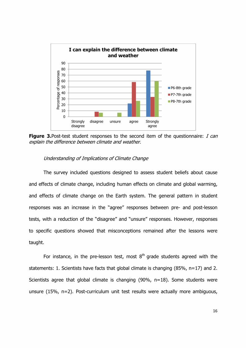
difference between climate and weather .............................................. 15 Figure 3. Post-test student responses to the second item of the questionnaire: I
can explain the difference between climate and weather ....................... 16 Figure 4. Subcategories of the correct responses category to the item "Do you
think sea level is different at different times? Why or why not? .............. 22 Figure 5. Example of one post-test response to the item "Do you think sea level
is the same everywhere? Explain and illustrate" .................................... 24 Figure 6. Balboa tide gauge sea level height series................................................... 39 Figure 7. Spectra of Balboa unfiltered time series (blue) and filtered time series
(red) .................................................................................................. 40 Figure 8. Frequency of non-tidal yearly grouped sea level events from Balboa
(a.) and Cristobal (b.) stations ............................................................. 43 Figure 9. Frequency histogram for the randomization test between sea level
maxima events at Balboa tide gauge and El Niño years ......................... 45 Figure 10. Global sea surface height anomaly in cm, derived from satellite
altimetry for the week of November 23 1994 ........................................ 47 Figure 11. Global sea surface height anomaly in cm, derived from satellite
altimetry for the week of December 3 1997 .......................................... 48
v
ABSTRACT
The present study had two main objectives. The first was to determine the degree of
understanding of climate change, sea level and sea level rise among middle school
students. Combining open-ended questions with likert-scaled questions, we identified
student conceptions on these topics in 86 students from 7th and 8th grades during 2012
and 2013 before and after implementing a Curriculum Unit (CU). Additional information
was obtained by adding drawings to the open-ended questions during the second year
to gauge how student conceptions varied from a verbal and a visual perspective.
Misconceptions were identified both pre- and post-CU among all the topics taught.
Students commonly used climate and climate change as synonyms, sea level was often
defined as water depth, and several students failed to understand the complexities that
determine changes in sea level due to wind, tides, and changes in sea surface
temperature. In general, 8th grade students demonstrated a better understanding of
these topics, as reflected in fewer apparent misconceptions after the CU. No previous
study had reported such improvement. This showed the value of implementing short
lessons. Using Piaget’s theories on cognitive development, the differences between 7th
and 8th grade students reflect a transition to a more mature level which allowed
students to comprehend more complex concepts that included multiple variables.

vi
The second objective was to determine if the frequency of sea level maxima not
associated with tides over the last 100 years increased in two tide gauges located on
the two extremes of the Panama canal, i.e. Balboa in the Pacific Ocean and Cristobal in
the Caribbean Sea. These records were compared to time series of regional sea surface
temperature, wind speed, atmospheric pressure, and El Niño-Southern Oscillation
(ENSO), to determine if these played a role as physical drivers of sea level at either
location. Neither record showed an increase in the frequency of sea level maxima
events. No parameter analyzed explained variability in sea level maxima in Cristobal.
There was a significant correlation between the zonal component of the wind and sea
level at Balboa for the early record (r=0.153; p-value<0.05), but for the most part the
p-values did not support the hypothesis of a correlation. Similarly, sea surface
temperature had an effect on sea level at Balboa, but the null hypothesis that there is
no correlation could not be rejected (p-value>0.05). There was a clear relationship
between sea level maxima and ENSO. 70% of the years with higher counts of higher
sea level events corresponded to El Niño years. A randomization test with 1000
iterations, shuffling the El Niño years, showed most of these randomizations grouped
between 14-35% of the events occurring during a randomized El Niño year. In no
iteration did the percentage of events that occurred during El Niño years rise above
65%. The correlation with zonal wind and the probable correlation with sea surface
temperature can be linked via ENSO, since ENSO is associated with changes in the
strength of the Trade Winds and positive anomalies in the sea surface temperature of
the tropical Pacific Ocean.
1
INTRODUCTION
One of the most pressing needs of society is to ensure some basic understanding
of the science behind climate change. This is important because these changes affect
the biosphere. This thesis had a dual purpose to address these concerns. One was to
understand the process of learning and education specifically using a case study of sea
level rise and climate change. The second objective was to better understand the tools
used in oceanography to measure sea level changes and to evaluate the possible
regional causes for trends in sea level change measured at any one locality.
The first chapter of this thesis has an educational focus. I assessed the
understanding of climate change, sea level, and sea level rise concepts in middle school
students at a middle school in the Tampa Bay area before and after a lesson unit on
climate and climate change. Baseline understanding on sea level and sea level rise was
measured in children. Then, new concepts were taught using oceanographic examples
based on real data from tide gauges located along the US coasts emphasizing the
Florida Coast near the region where the students live. Learning focused on sea level rise
occurring over the course of the past several decades. Students were also allowed to
utilize other real data to develop products that facilitated the understanding of this topic
by the use of simple examples and hands-on exercises, which were effective as
teaching tools for these children.

2
The second chapter of the thesis is based on a time series analysis of sea level
records off the Panama Canal to test the hypothesis that maxima in sea level not
associated to tides were increasing in occurrence. We used tide gauge records from
Balboa in the Pacific Ocean and from Cristobal in the Caribbean Sea to evaluate short-
term (days) to interannual variation in sea level. Sea level data were compared to
regional changes in temperature, wind speed, and atmospheric pressure in an effort to
understand what controls sea level changes at both ends of the Panama Canal. The
study was useful to learn time series data processing methods. We looked for changes
in the occurrence of extreme sea level events but found no such trend. Marked maxima
in sea level occurred in conjunction with other oceanographic phenomena, such as El-
Niño-Southern-Oscillation events. The study helped better understand variability in sea
level in the region.
3
CHAPTER 1
MEASURING MIDDLE SCHOOL STUDENT UNDERSTANDING OF CLIMATE CHANGE, SEA
LEVEL AND SEA LEVEL RISE
INTRODUCTION
Coastal areas of the world are densely populated, with about 10% of the
population or 600 million people living in coastal flood plains and island regions
(McGranahan et al. 2007; Alley et al. 2005). These areas are directly exposed to short
and long-term sea level changes that have important social and economic impacts
(Milne et al. 2009; Church et al. 2008; Anthoff et al. 2006; Small and Nicholls 2003). A
public that understands this dynamic environment can make better decisions and more
effective use of the coastal zone.
Here we describe an effort to assess progress in understanding complex Earth
science issues in middle school age children. The program focused on understanding of
sea level change. The effort was conducted jointly between a large research institution
in the southeastern United States and a Florida magnet middle school. The strategy
consisted of engaging school students in authentic science research projects led by
scientists and their graduate students. This model presents students a chance of
learning how science is being done by participating on some of the research themselves

4
in an inquiry-based educational approach (Feldman et al, 2012). The student
interactions with faculty and graduate students provided first-hand experience of
possible career paths in science as they learned about earth processes that have
impacts on their communities.
Sea level rise is relevant to residents in Florida Peninsula, where communities are
located in low-lying areas only a few feet above sea level up to 60 miles inland, with the
Atlantic Ocean or the Gulf of Mexico surrounding most of the state (Hauserman, 2007).
Few Floridians are exposed to basic ocean science concepts during their formative
years. For instance, the words “sea level rise” are not in the National Science Education
Standards (1996), in the Benchmarks for Science Literacy (1993), or in the Florida Next
Generation Sunshine State Standards (2008). This could change if the Framework for K-
12 Science Education (2012) were to be adopted. These standards include some
general topics on global climate change and sea level. The Next Generation Science
Standards (NGSS) (2013) review some of the science concepts to provide adequate
knowledge on climate change and sea level.
Climate change is a topic widely discussed in different sectors of society. It is
important for students to have an understanding of the concepts that underlie these
discussions since they are carried out in regional, national and international politics, and
to be cognizant of their societal relevance.
Some studies have attempted to evaluate student conceptions of climate change
at middle, high school, and college level (Herman, 2015; McNeill and Vaughn, 2012;
Shepardson, 2009; Cordero et al., 2008; Kilinc et al., 2008; Anderson and Wallin, 2000;
5
Koulaidis and Christidou, 1999; Rye et al., 1997; Boyes et al, 1993). Herman (2015)
working with 324 high school students from a marine science section, tried to
understand their views on global warming and their willingness to engage on mitigating
activities. He determined the socio-cultural factors and views regarding global warming
become less relevant as the mitigating actions required more self-sacrifice. Additionally,
students' perception on global warming science methods influenced their participation
in mitigation activities. Ethnicity and socio-cultural classification were found to be
important on students' inclination to mitigate global warming. McNeill and Vaughn
(2012) focused on high school student understanding and beliefs about climate change
in a four to six week urban ecology curriculum. Pre- and post-assessments showed that
at the beginning of the course most of the students believed climate change was
occurring. After the course, most students had developed actual understanding of the
subject and became engaged in environmental activities designed to mitigate its
impacts. Kilinc et al. (2008) found that a large percentage of high school students
surveyed considered melting polar ice caps (95%) and flooding (71%) to be direct
consequences of global warming. However, they found misconceptions and confusion
about the causes and effects of climate change.
Shepardson et al. (2009) and Rye et al. (1997) explored conceptions of global
warming and climate change in seventh grade students. Shepardson et al. reviewed 16
international research studies that focused on the greenhouse effect, global warming,
and climate change. They found few works that focused exclusively on seventh grade.
The findings of their study were that students lacked a rich conceptualization of the

6
issues. They also found that the students did not understand the impact of climate
change on the oceans, weather, animals and plants. Rye et al. (1997) found that a
majority of the students had conceptions that mixed up concepts of global warming,
greenhouse gas effects, and ozone layer depletion after completion of one of the six
Science-Technology-Society (STS) units on global warming.
In this study, our interest was specifically on sea level and sea level rise. The
literature on these topics is for the most part limited to lesson plans and diverse
teaching hands-on activities like those included in the work of Gillette and Hamilton
(2011), Oguz (2009), and Bugg et al. (2007). We found no studies that specifically
target knowledge about sea level and sea level rise, or how these may be related to
climate change.
Our objective was to measure change understanding climate change in a middle
school setting using visualizations of sea level rise. We analyzed perceptions about the
definition of “sea level” and concepts about sea level rise, and its relationship to climate
change. We conducted surveys before and after a two weeks curriculum unit on sea
level change conducted as part of a larger Earth Science curriculum in a middle-grade
school with 7th and 8th grade students during 2012 and 2013. We encountered
misconceptions related to most related topics before and after the process. However, in
general, 8th grade student responses were more accurate than those from 7th grade
students. This suggested a better conceptual understanding of the complex Earth
system processes with age.
7
METHODS
Project Curriculum Unit
We used sea level data from local, regional and national tide gauges paired with
geological evidence and theoretical information on sea level and sea level rise as tools
to teach about climate change. A curriculum unit (CU) was developed and implemented
for each year (Table 1). This CU used simple examples and hands-on activities to
illustrate basic concepts. The first part of the CU focused on a theoretical and
conceptual basis of climate change, and established the difference between 'weather'
and 'climate'.
The CU also addressed expressions and impacts of climate change in time and in
space, and specifically how these processes affect coastal sea level. The lessons
included long-term and short-term changes (glacial and interglacial periods) and the
concept of forcing of climate change due to human activities. For the final part of the
CU students used real tide gauge data from US tide gauges. Basic analysis was
accomplished with the use of spreadsheet applications. Students had the opportunity to
visualize sea level trend at different locations and based on the lessons and their
observations they postulated possible future scenarios. At this point the lesson included
a discussion on the complexity of the models used to predict future sea level rise and
the uncertainty related to such predictions. Classroom observations of student reactions
and verbal responses during the lessons were used as qualitative data. A detailed
description of classroom activities developed is presented in Appendix A.

8
Table 1. Lessons, concepts and activities included in the curriculum unit implemented in the present study.
LESSON NAME CONCEPTS DISCUSSED ACTIVITIES
1. CLIMATE VS
WEATHER
(1-2 periods)
a. Introduction to the basic concepts needed
for subsequent lessons (climate, weather,
climate change, sea level)
b. Differences in sea level change due to ice
melting on land and melting sea ice.
c. Global warming or climate change, what is
the difference? The consequences of change
in terms of sea level.
Melting ice experiment.
Global climate change
warming reading
materials.
2. GLACIAL VS
INTERGLACIAL
Ancient sea level
(2 periods)
a. Evidence of climate change in the geologic
past (glacial and interglacial periods).
b. Ancient sea level, why and how did sea
level change?
c. Ancient CO2 concentration and
temperature and their relationship to climate
change.
North America map, sea
level changes in
geological history.
3. SEA LEVEL AND SEA
LEVEL RISE
(2 periods)
a. Definition of sea level and mean sea level.
b. Importance of reference points for
measuring sea level. Tides.
c. Sea level rise from the last glacial
maximum and over the past 100 years.
d. Ice melting and thermal expansion.
e. Measuring sea level change: Tide gauges
and satellites.
“What forces change
sea level?” Hands-on
activity.
Thermal expansion.
Exercise: “Let’s become
water molecules”.
4. FUTURE SEA LEVEL
(3-4 periods)
a. Data: analysis and interpretation – can we
use past change to forecast the future?
b. Sea level rise prediction: limitations and
uncertainties of the models.
c. Understanding data from US tide gauges.
Tide gauge data
analysis. Data from US
coastal tide gauges.
Participants
A total of 86 7th and 8th grade students took part in the research. Specifically,
two 7th grade (P7, n=13 and P8, n=15) and one 8th grade (P6, n= 20) classes
participated during 2012, and one 7th and one 8th grade class were involved during
9
2013 (P4, n=23 and P1, n=15). All students were part of a Marine Science elective at a
magnet middle school in the southeastern United States, recognized as a NASA Explorer
School with a focus on science, technology, engineering and mathematics (STEM)
education.
Assessment of Change in Understanding
A survey with three open-ended items and 20 multiple choice items was
designed and implemented by a group of science educators, graduate students, and
marine scientists. Part of the survey tool focused on understanding of the scientific
method. To properly design the survey questions specific to sea level, eight students
were interviewed before the process started. Responses were used to develop a set of
seven open-ended and two multiple-choice items. Preliminary results from the 2012
study group were also used to modify the instrument prior to its use with the 2013
study group. This led to replacing the earlier instrument with five new open-ended and
illustration items that provided an opportunity to collect more detailed responses. The
instrument was implemented twice, before and after the curriculum unit was taught
each year. This study was approved by the university’s institutional review board (IRB).
Data Analysis
Qualitative data analysis was performed based on Patton (1990). Most multiple-
choice items followed a 5-point Likert scale (strongly disagree, disagree, unsure, agree
10
and strongly agree). Descriptive statistics were used to interpret the results from those
items relevant to the present study. Responses to the open-ended items were
transcribed verbatim and a label was assigned to each survey including period number,
student consecutive number, and pre- or post-test timeframe (e.g. P6-3-Pr, P8-1-Po) to
preserve anonymity. Initial analysis of the 2012 pre-test results was done without
regard of class period. Responses were separated into categories following Patton
(1990), based on pre- and post-test responses. Each response was discussed among
the researchers and grouped into the respective category according to a consensus
among researchers. Inductive analysis was conducted and differences between the pre-
and post-test were analyzed for each class group; misconceptions and positive changes
in conceptual understanding were identified. Preliminary results identified ambiguous
responses that prevented the categorization of many of the student responses about
their understanding of sea level and sea level rise.
Rubrics
The questionnaire implemented for 2013 included open-ended items that had to
be complemented with a drawing. Figure 1 shows an example of a drawing submitted
by a student. A rubric was constructed for each written item, and another rubric
addressed the illustrations. The goal was to determine whether each supported,
contradicted, or was relevant at all to the written answer. A third rubric was constructed
to assess the response as a whole (see DeBoer et al., 2008). Appendix B includes the
rubrics constructed for the 2013 questionnaire.

11
Figure 1. Example of one response including a detailed illustration to the question: “What is sea level? Define, draw and label”.
A numerical value was assigned to each response. The highest values
corresponded to more elaborated or complete responses. A value of zero corresponded
to an absent, incomplete, or inaccurate response. Results are presented here as
percentage values, to facilitate comparison among groups.
RESULTS
Understanding Climate Change
A comparative measure of how students understood climate change was
determined from the survey responses. The first question was “What is climate
change?” The intent was to assess general knowledge without leading student
reasoning. We used a simplified definition of climate change based on the formal
definitions found in the IPCC report (2007) for weather, climate, and climate change.
Specifically, climate change was defined as: changes in the average weather and/or the
12
variability of it properties that persist for an extended period, typically decades or
longer. The World Meteorological Organization and therefore meteorologists around the
world use the average of weather parameters over a period of 30 years a practical
definition of climate (IPCC, 2007). Change is thus evaluated from standard 30-year
period to the next 30-year period. This type of definition was discussed during the
lessons, with the explanation that we often need a reference point to help people
understand concepts of change, i.e. that require comparisons over different time
frames.
An adequate student response to "What is climate change?" should in principle
address at least two concepts: 1) Differentiate between climate and weather, and 2)
Consider a timeframe over which to consider each concept. Responses were evaluated
as either adequate or inadequate depending on whether students grasped the concept
of short or long timeframes. Inadequate responses included those that showed no such
understanding, or surveys that had no response. Criteria used to define categories are
included in Table 2.
Table 3 summarizes responses for the survey item “What is climate change?”
(first item). Pre-tests results were similar among the various groups, with 64-80% of
responses shown as inadequate. Students showed that in general they had “built in”
misconceptions. The main problem was that they thought of climate, weather, and
temperature as synonyms, and that they did not have a sense of a timeframe
component in their responses. These misconceptions were also seen in some of the

13
“adequate” responses, which thus were only partly correct. Some examples of
incomplete responses to the question of "What is Climate Change" included:
-It is when the temperature or climate changes (P6-4-Pr)
-Change in weather (P8-13-Pr)
-The change in seasons? Temperature (P6-6-Pr)
Post-curriculum unit results showed an increase to 84% adequate responses
among 8th grade students. Many students remained confused about the concept of
"time" in terms of decades.
Table 2. Categories for assessing the survey item “What is climate change?” Responses were grouped in to two main categories (Inadequate and Adequate) and seven subcategories.
INADEQUATE ADEQUATE
No answer Student provided no
answer
Time correct Student responses
includes the time
component of the
definition correctly
(short or long period of
time)
I do not know Student specifically
stated IDK (I don’t
know)
Climate correct Student’s response
defined climate
correctly in terms of
weather and timeframe
Incorrect Student’s response did
not fit the accepted
definition
Correct The response fulfilled the
definition in terms of
weather and time
requirements
Tautology Student's response was
the same as the
question but with
words rearranged
On the other hand, 60-67% of 7th grade students showed inadequate responses
even after the lessons from the curriculum unit. They also had new misconceptions,

14
such as: 1) Climate is a synonym of climate change, and 2) climate is extremes in
weather or the average weather, but not both.
From classroom observations and the written responses it was clear that
students were impressed to learn that one needed several decades (like 30 years) to
obtain some measure of climate. This generated the most confusion among 7th grade
students, as the following examples illustrate:
-It is the extremes over a long period of time (about 30 years) (P7-8-Po)
-Change in the weather over 30 years and dramatic changes like storms, earthquakes, and icebergs (P8-6-Po)
-The change in weather after 30 years (P8-15-Po)
The second item in the questionnaire asked how much a student agreed or
disagreed with the statement: “I can explain the difference between climate and
weather”. 50 to 80% of students agreed or strongly agreed with the statement before
the lessons (Figure 2).
Table 3. Percentage of responses per category to the question: What is climate change? Bolded values correspond to the highest percentage for the test.
P6 8TH GRADE P7 7TH GRADE P8 7TH GRADE
Category Subcategory Pre-test Post-test Pre-test Post-test Pre-test Post-test
No answer - - 15 - - -
Inadequate I don’t know - - - - - -
Incorrect 60 11 54 59 50 60
Tautology 20 5 8 8 14 -
Time correct 5 - - - 7 -
Adequate Climate correct 5 28 8 8 7 -
Correct 10 56 15 25 22 40
N 20 18 13 12 14 15

15
After participation in the lessons and hands-on activities, students became more
aware of the differences between climate and weather. This is apparent in their post-
lesson responses (Figure 3). However, it is also apparent that a student’s beliefs about
what they know (i.e. what they think they know) does not necessarily mean that they
have proper conceptual understanding. Such problems of misconceptions were largest
among 7th grade students.
Figure 2.Pre-test student responses to the question: I can explain the difference between climate and weather.
0
10
20
30
40
50
60
Strongly disagree
disagree unsure agree Strongly agree
Perc
enta
ge o
f re
sponse
s
I can explain the difference between climate and weather
P6-8th grade
P7-7th grade
P8-7th grade
16
Figure 3.Post-test student responses to the second item of the questionnaire: I can explain the difference between climate and weather.
Understanding of Implications of Climate Change
The survey included questions designed to assess student beliefs about cause
and effects of climate change, including human effects on climate and global warming,
and effects of climate change on the Earth system. The general pattern in student
responses was an increase in the “agree” responses between pre- and post-lesson
tests, with a reduction of the “disagree” and “unsure” responses. However, responses
to specific questions showed that misconceptions remained after the lessons were
taught.
For instance, in the pre-lesson test, most 8th grade students agreed with the
statements: 1. Scientists have facts that global climate is changing (85%, n=17) and 2.
Scientists agree that global climate is changing (90%, n=18). Some students were
unsure (15%, n=2). Post-curriculum unit test results were actually more ambiguous,
0
10
20
30
40
50
60
70
80
90
Strongly disagree
disagree unsure agree Strongly agree
Perc
enta
ge o
f re
sponse
s
I can explain the difference between climate and weather
P6-8th grade
P7-7th grade
P8-7th grade

17
with 89% (n=16) of responses agreeing with the first statement, only 66% (n=12)
agreeing with the second statement, and 12% (n=2) disagreeing.
Questions about the consequences of climate change showed some basic
misconceptions. For example, responses to the question: “Global warming causes
droughts or floods”, showed that more than 30% of P8 students (7th grade) were
“unsure” or “disagreed” after the lessons. In the Post-lesson test, most P8 students (7th
grade) disagreed (34%, n=5) or were unsure (20%, n=3) and 25% (n=3) of P7
students (7th grade) disagreed with the statement. Most 8th grade student responses
reflected a better understanding of the concepts, a lower tendency to retain erroneous
concepts, and an ability to learn and show increased understanding through the
lessons. Given strong emphasis on sea level throughout the curriculum unit, the
complexity and range of possible consequences of climate change will likely remain
outside the grasp of middle school students.
Understanding Sea Level
Sea level is defined by the Oxford English Dictionary as: “the level of the surface
of the sea with respect to the land, taken to be the mean level between high and low
tide, and used as a standard base for measuring heights and depths” The IPCC report
(2007) includes a formal definition of relative sea level as: " Sea level measured by a
tide gauge with respect to the land upon which it is situated. Mean Sea Level (MSL) is
normally defined as the average Relative Sea Level over a period, such as a month or a
year, long enough to average out transients such as waves". We assessed student
18
understanding about sea level and sea level rise and identified a number of
misconceptions.
The most common misconception was that sea level is “the height of the sea”
without a reference against which to measure height, i.e. the land (40, 39 and 22% of
the pre test responses; Table 4). Examples of responses follow:
-The depth of the sea in relation to the land and shores (P6-9-Pr)[it is not clear whether this answer shows understanding or not; technically it is correct]
-The height of the sea compared to the land (P6-13-Pr; correct)
-Sea level is where the point of the water of the sea stops and the land continues (P8-8-Pr; correct)
“Global mean sea level” was another concept we explored, to gauge how
students related local concepts to the entire ocean. Pre-curriculum unit test results for
the question “What is global mean sea level? “ showed a large number of
misconceptions (40-47%) or “I don’t know” (39%) responses. Post-curriculum unit test
results showed an increase in understanding, with 8th grade students showing a higher
rate of correct responses compared to 7th grade responses. Upwards of 50% of the P7
student (7th grade) post-curriculum unit responses remained incorrect. (Table 5).

19
Table 4. Percentage of responses per category to the question: What is sea level? for pre-curriculum unit and post-curriculum unit tests. Bold values show the highest percentage for the test.
P6 8TH GRADE P7 7TH GRADE P8 7TH GRADE
Category Pre-test Post-test Pre-test Post-test Pre-test Post-test
Height of the sea 40 29 39 34 22 46
Tautology 20 12 - 18 14 -
Where there is water/ no land 5 - - - - 7
Top or surface of the water 5 - - 9 7 -
Incorrect 10 - 23 34 21 33
Correct 5 47 15 - 29 7
Ocean depth 5 12 15 - - -
Average level 10 - - - - -
Amount of water - - 8 9 7 7
N 20 18 13 12 14 15
Table 5. Percentage of responses per category to the question: What is global mean sea level? Bold values correspond to the highest percentage for the test.
P6 8TH GRADE P7 7TH GRADE P8 7TH GRADE
Category Pre-test Post-test Pre-test Post-test Pre-test Post-test
No answer - - 32 - 14 27
I do not know - - 7 8 36 -
Correct 40 61 7 25 29 46
Average sea/ incomplete 20 11 7 17 - 27
Incorrect 40 28 47 50 21 -
N 20 18 13 12 14 15
The item "Do you think sea level is the same everywhere on Earth? Why or why
not?" had a large number of responses that showed misconceptions (Table 6). For
example, student responses included references to the Moon-Earth-Sun system, melting
sea ice, or volume displaced by sea animals:
20
-No because the moon can be stronger in other places, because of the tilt on the axis on the Earth (P8-5-Pr; incorrect)
-No because the sea creatures put presher [sic] in the water making it rise (P8-14-Pr; incorrect)
-No it can be higher in the Artic because of the icebergs melting (P6-20-Pr; incorrect)
Another common misconception was defining sea level as the depth of the water
column:
-No because the sea bottom is deeper in some places (P6-12-Pr; inaccurate)
Or misapplication of a scientific principle:
-Yes because earth's oceans are connected (P7-7-Pr; inaccurate)
Post-curriculum unit test results showed an increase in the correct responses in
all groups, but misconceptions remained:
-Yes, because even though it is hot somewhere and ice is melting in other places it all evens out (P6-15-Po)

21
Table 6. Percentage of responses per category to the question: Do you think sea level is the same everywhere on Earth? Why or why not? Bold values correspond to the highest percentage for the test.
P6 8TH GRADE P7 7TH GRADE P8 7TH GRADE
Category Subcategory Pretest Posttest Pretest Posttest Pretest Posttest
No answer - - 8 - - -
I don’t know 5 - 8 - - -
Affirmative Incorrect 10 22 15 - 36 6
Incomplete 5 5 8 17 14 -
Seas connected 30 - 15 - 7 -
Different seas 10 - - - - -
Negative Different depths 25 17 23 8 29 27
Different levels - - 23 - - -
Correct 15 56 - 75 14 67
N 20 18 13 12 14 15
Table 7 summarizes the results on the item: "Do you think sea level is different
at different times? Why or why not?” Pre- and post-tests gave similar results.
Table 7. Percentage of responses per category to the question: Do you think sea level is different at different times? Why or why not? Bold values correspond to the highest percentage for the test.
P6 8TH GRADE P7 7TH GRADE P8 7TH GRADE
Category Pretest Posttest Pretest Posttest Pretest Posttest
No answer - - 15 - - 7
I don’t know - - 8 - - -
Incorrect 15 11 15 - 22 13
Incomplete 5 - - 25 14 20
Correct 80 89 62 75 64 60
N 20 18 13 12 14 15
Most students had a good understanding that the sea level changes over time. In
this regard, 8th grade students (P6) had the most “correct” responses (80-89%), but

22
misconceptions were present among all groups even post-lessons. Figure 4 shows the
frequency of the different responses for the pre and post-curriculum unit tests. Tides
and waves were the most common response in both tests for all groups, whereas
interglacial/glacial was only mentioned by one P6 student in the post-curriculum unit
test.
One item sought to understand student beliefs about how different processes
might affect sea level, namely wind, tides, storms, melting ice, and temperature. All
student responses about each process showed similar results, with a higher percentage
of correct responses in the post-curriculum unit test compared to the pre-curriculum
unit test. Again, more correct responses were given by 8th grade students (90%) than
by 7th grade students (60%).
Figure 4. Subcategories of the correct responses category to the item Do you think sea level is different at different times? Why or why not? P6 corresponds to 8th grade students; P7 and P8 correspond to 7th grade students.
0
2
4
6
8
10
12
Num
ber
of
resp
onse
s
Pre-test P6
Pre-test P7
Pre-test P8
Post-test P6
Post-test P7
Post-test P8

23
Student responses to how "wind" acts on sea level indicated poor understanding
of this process. Some misconceptions were identified, for instance one student
responded "Erosion". This seemed to be due to confusion of what happens in nature,
such as shown in the post-curriculum unit test response: "erode shores" and "Yes,
erosion the land, causing it to sink". Few students understood the effect of “surge” or
the role of “waves” formed by wind (any mention to water movement due to wind was
accepted). The general misconception was that winds have no effect on sea level:
Pre-curriculum unit test Post-curriculum unit test
No wind can't blow water away (P6-5-Pr) No, air not water moving (P6-1-Po)
No, because it will just push water (P7-7-Pr) no cus [sic] it just moves it around (P7-
1-Po)
No because wind is air (P8-13-Pr) No because it isn't doing anything to
change it (P8-10-Po)
Other misconceptions included considering that storms can affect sea level more
by carrying water around as rain than pushing water from or away from shore (storm
surge), that temperature (heat) does not play a role in sea level, or how melting ice
(glacier ice vs. sea-ice) affects sea level. Despite a general improvement in the post-
curriculum unit responses, misconceptions remained.
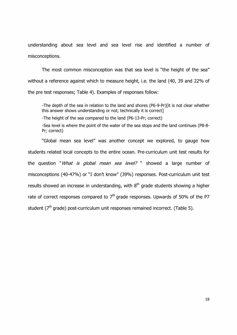
Results from the 2013 surveys showed that illustrations by students helped them
to communicate their conceptions and avoid misconceptions. Several students showed
difficulties with a written definition but showed acceptable illustrations. For example 9%
24
of 7th grade students had a correct written response but 39% provided a satisfactory
drawings of a sea level conceptualization, including a land reference. For 8th grade
students, 29% showed correct responses and 50% satisfactory drawings. In some
cases, the written responses were accurate and the illustrations were more confused
(Figure 5, where the overall caption seems generally correct, but the arrow points to a
small ocean with a changing sea level due to a whirlpool).
Figure 5. Example of one post-test response to the item “Do you think sea level is the same everywhere? Explain and illustrate” .The written response is correct however the illustration does not support the statement and may be considered contradictory.
The results of the first item: "What is sea level? Illustrate” were very similar to
those from the 2012 process for written responses. 8th grade students (P1) responses
reflected a better understanding than that of 7th grade students (P4), but both groups
presented misconceptions in the post-curriculum unit test. When illustrations were
considered independently, the results improved for both groups, however some
illustrations contradicted the written responses, leading to lower overall response
quality (Table 8).
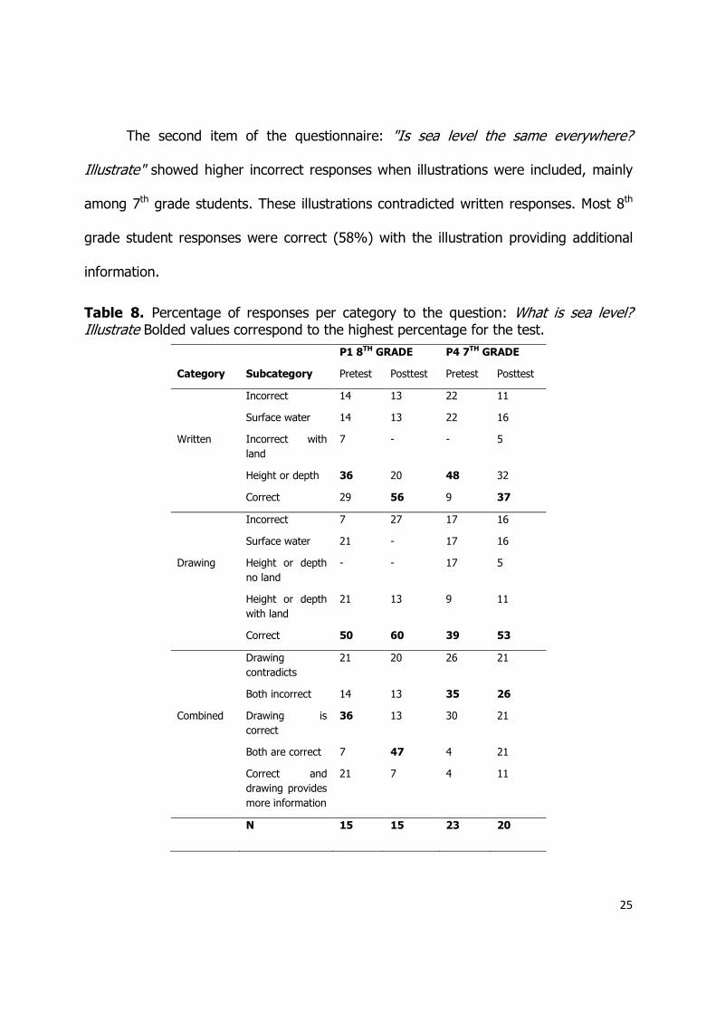
25
The second item of the questionnaire: "Is sea level the same everywhere?
Illustrate" showed higher incorrect responses when illustrations were included, mainly
among 7th grade students. These illustrations contradicted written responses. Most 8th
grade student responses were correct (58%) with the illustration providing additional
information.
Table 8. Percentage of responses per category to the question: What is sea level? Illustrate Bolded values correspond to the highest percentage for the test.
P1 8TH GRADE P4 7TH GRADE
Category Subcategory Pretest Posttest Pretest Posttest
Incorrect 14 13 22 11
Surface water 14 13 22 16
Written Incorrect with
land
7 - - 5
Height or depth 36 20 48 32
Correct 29 56 9 37
Incorrect 7 27 17 16
Surface water 21 - 17 16
Drawing Height or depth
no land
- - 17 5
Height or depth
with land
21 13 9 11
Correct 50 60 39 53
Drawing
contradicts
21 20 26 21
Both incorrect 14 13 35 26
Combined Drawing is
correct
36 13 30 21
Both are correct 7 47 4 21
Correct and
drawing provides
more information
21 7 4 11
N 15 15 23 20

26
The third item: "Is sea level the same all the time? Illustrate". Most students
provided a good response to this item, with over 50% correct responses in the pre-
curriculum unit test. The post-curriculum unit written test responses improved to nearly
60%, and the combined correct responses (written and illustration) reached 75% in the
post-curriculum unit test (7th grade students). In the post-curriculum unit test, no 8th
grade student responses were incorrect whereas 15% of 7th grade student responses
were incorrect or included misconceptions.
DISCUSSION
Perceptions and Understanding Climate Change
It is useful to understand how we develop perceptions of natural phenomena,
time, and over scales that span from our local surroundings to the Earth as a system. It
is also useful to understand how scientific information is absorbed by children at
different stages of education. In this study, groups of middle school children were
presented with scientific information about sea level and how climate change may affect
sea level. The students were asked about their perception of time, climate change, and
sea level before and after scientific information was presented to them.
Two items in the pre-curriculum unit questionnaire were related to weather,
climate, and climate change. Results showed that most students were better prepared
to differentiate between weather and climate after the learning process. However, in

27
practice, 8th grade students demonstrated better assimilation of information by
providing more reasonable concepts about climate change. While 7th grade students
displayed increased confidence about what they had learned, they did not seem to
understand the information given to them compared to the 8th grade students. They
showed misconceptions even after the teaching sessions.
Other researchers have found that middle-school children hold substantial
misconceptions about climate change. For example, Shepardson et al. (2009) found
that most seventh grade students expect that sea level will rise as a consequence of
polar ice melting due to global warming, and that a third think that sea level will
decrease because of more evaporation. These concepts seem to be developed without
clear reasoning of natural processes or understanding the geographic or time scale over
which things would happen. Kilinc et al. (2008) found that Turkish high school students
have a good understanding of the physical consequences of global warming. This was
attributed to instruction and media images. Cordero et al. (2008) worked with large
groups of undergraduate students (n=470), who understood that there is a link
between global warming, melting polar ice, and sea level rise, even though it is clear
that they don’t understand the complex mechanisms acting on each of these processes.
Jakobsson et al. (2009) working with 14-15 year-old students, used direct observations
rather than written questionnaires and found that after a six-week program, students
began to use scientific vocabulary and were more comfortable reaching reasonable
conclusions about complex Earth and climate processes.

28
Our results show that the use of scientific data about specific natural processes is
not sufficient to guarantee understanding of these Earth system processes. Processes
related to climate are extremely complex and it is not easy for any one person to
comprehend the time and space scales over which they operate. Even reducing the
problem to a few variables such as sea level and sea level rise is difficult to understand
to 7th grade students. There is a marked improvement in the rate to understand and
explain such complex concepts one year later, as students reach 8th grade.
Regarding climate change, it is important to engage students in activities
oriented to develop a personal connection with the concepts to promote a better
disposition and learning experience (Cordero et al., 2008). In general, students struggle
to differentiate between short and long-term processes (McNeill & Vaughn, 2012). A
look at the work of Jean Piaget (Pulaski, 1971) might be useful for understanding why
we saw this. Piaget's theory of children’s cognitive development establishes a series of
requirements that set intellectual development in motion, namely: maturation,
experience and social transmission. According to Piaget, these requirements create the
necessary stimulus for children to achieve higher stages of cognitive levels. Piaget also
defined stages of learning that children go through based on learning capabilities and
development. As they advance in age and grade, students are able to understand more
complex and even hypothetical and abstract concepts, including basic mathematical
models. Piaget theorized that children at around age 11 or 12 transition to a
developmental stage in which they can comprehend concepts that include multiple
variables, such as climate change.

29
Our results support the idea that more mature students grasped Earth science
concepts more easily, acquiring a better understanding and incorporating the adequate
vocabulary as part of their responses. It is possible that the differences in our results
between 7th and 8th grade students may have been due to their transition from one a
lower stage of cognitive development to a higher stage. However, it is also possible that
the differences could be due to an additional year of schooling rather than the type of
cognitive development hypothesized by Piaget.
Understanding Implications of Climate Change
The portion of the pre-curriculum unit questionnaire that addressed the level of
student agreement or disagreement to statements related to climate change had
ambiguous results. However, this was expected given the emphasis of the curriculum
unit on the narrower topics of sea level and sea level rise. There is little in the local or
national standards that focuses on the local impacts of global climate change. As a
result, this curriculum unit did not have much influence the student conceptions or
beliefs. Nevertheless, students that participated in the focused teaching and learning
experience met scientists that are engaged in studying climate change, and they were
able to see the substantial agreement among scientists on this issue.
Students typically come into school with pre-instructional knowledge that is often
based on preconceptions and incorrect conceptions (Duit & Treagust, 2003). Duit and
Treagust (2003) found that it was difficult to replace those misconceptions even after
offering evidence to the contrary. Student motivation, affective resistance, and beliefs

30
further complicate this process (Sinatra & Pintrich, 2003). Based on some in class
responses and students attitudes it is possible that some of these preconceptions were
acquired from student parents before the curriculum unit was implemented, and was
reflected in the responses, specially the pre-curriculum unit tests.
We found similar differences in the understanding of the concepts between 7th
and 8th grade students in both years that the curriculum unit was implemented. Older
students were more likely to understand the new concepts, fitting Piaget's theory.
Nevertheless misconceptions were still present among all groups even after instruction.
Most likely, the short unit provided insufficient exposure to the complex topics of
climate change and sea level. Our results suggest that most students do not understand
the definition of sea level or the basic natural processes that lead to sea level changes.
It is also clear that students have alternative conceptions that are used when
they try to understand something new, and often those ideas are incompatible and
unrelated to school science (Anderson & Wallin, 2000). These conceptions have been
shown to remain even after formal instruction has been imparted and can have a
negative impact in children's fully understanding of a series of more elaborated
concepts that rely in the basic principles.
The curriculum unit included practical work with real sea level data from local
and remote tide gauges. Students saw sea level changes over short (tide) and long
(decadal) time scales, and yet most students failed to internalize change in sea level as
part of their responses. Students participating in real science experiments and
experiences should modify their vocabulary and understanding to be more scientifically
31
accurate (Jakobsson et al., 2009). But in practice, this is a slow and continuous process
that requires repetitive experiences to help clear previous misconceived concepts
(Kuhn, 1970). The process of acquisition and implementation of scientific vocabulary is
gradual and requires time (McNeill & Vaughn, 2012; Jackobson et al., 2009).
Our results lead to the following recommendations for further research:
1. Modifying the duration of the lesson plans (i.e. providing repetitive experiences
over a longer period); this may help minimize misconceptions and allow more
mature understanding to develop (McNeill and Vaughn's approach; 2012).
2. Test whether the differences observed between 7th and 8th grade students are
due to differences in the developmental stages following Piaget's ideas or to the
lesson plans offered to the different grade levels.
3. Finally, develop strategies to introduce basic concepts on how global Earth
processes change and affect local processes such as sea level early in the
curriculum, to help prevent the development of misconceptions that can become
deeply rooted in a person’s conceptual framework.
REFERENCES
AAAS, 1993: Benchmarks for science literacy. NY: Oxford University Press.
Alley, R., P. Clark, P. Huybrechts and I. Joughin, 2005: Ice-Sheet and Sea-Level
Changes. Science, 310, 456-460.

32
Anderson, B. and A. Wallin, 2000: Students' Understanding of the Greenhouse Effect,
the Societal Consequences of Reducing CO2 Emissions and the Problem of Ozone
Layer Depletion. J. Res. Sci. Teach. 37(10), 1096-1111.
Anthoff D., Nicholls R.J., Tol R.S.J. and A.T. Vafeidis, 2006:Global and regional
exposure to large rises in sea-level: a sensitivity analysis. Tyndall Centre for
climate change Research Working paper 96.
Boyes, E., Chuckran, D. and M. Stanisstreet, 1993: How Do High School Students
Perceive Global Climatic Change: What Are Its Manifestations? What Are Its
Origins? What Corrective Action Can Be Taken?. J. Sci. Educ. Technol. 2(4), 541-
557.
Bugg, S.R., Constible, J., Kaput, M. and R.E. Lee, 2007: They're M-e-e-elting!: An
Investigation of Glacial Retreat in Antarctica. Sci. Scope. 30(5), 42-48.
Church, J.A., White, N.J., Hunter, J.R. and K. Lambeck, 2008: A post-IPCC AR4 update
on sea level rise. Antarctic Climate and Ecosystems Cooperative Research Centre,
Hobart.
Cordero, E.C., Todd, A.M. and D. Abellera, 2008: Climate change education and the
ecological footprint. Bull. Amer. Meteor. Soc. 89(6), 865-872.
Duit, R. and D.F. Treagust, 2003: Conceptual change: A powerful framework for
improving science teaching and learning. Int. J. Sci. Educ., 25(6), 671-688.
Feldman, A., Chapman, A., Vernaza-Hernandez, V., Ozalp, D. and F. Alshehri, 2012:
Inquiry-based science education as multiple outcome interdisciplinary research
and learning (MOIRL). Sci. Ed. Int. 23(4), 328-337.

33
Florida Department of Education, 2008: Science Next Generation Sunshine State
Standards from http://www.floridastandars.org
Gillette, B. and C. Hamilton, 2011: Flooded! An Investigation of Sea-Level Rise in a
Changing Climate. Sci. Scope. 34(7), 25-31.
Hallden, O., 1999: Conceptual change and contextualization. In Schnotz, W.,
Vosniadou, S. and M. Carretero (Eds.), New Perspectives on Conceptual Change.
Oxford: Pergamon, Elsevier Science. 53-65.
Hauserman, J., 2007: Florida's Coastal and Ocean Future. A Blueprint for Economic and
Environmental Leadership. Natural Resources Defense Council Inc.
Herman, B., 2015: The influence of global warming science views and sociocultural
factors on willingness to mitigate global warming. Sci Ed. 99(1), 1-38.
Jakobsson, A., Makitalo, A. and R. Saljo, 2009: Conceptions of Knowledge in Research
on Students' Understanding of the Greenhouse Effect: Methodological Positions
and Their Consequences for Representations of Knowing. Sci. Educ. 93(6), 978-
995.
Kilinc, A., Stanisstreet, M. and E. Boyes, 2008: Turkish students' ideas about global
warming. Int. J. Environ. Sci. Educ. 3(2), 89-98.
Koulaidis, V. and V. Christidou, 1999: Models of Students' Thinking Concerning to
Greenhouse Effect and Teaching Implications. Sci. Educ. 83(5), 559-576.
Kuhn, T.S., 1970: The Structure of Scientific Revolutions. Chicago: Chicago University
Press.

34
McGranahan, G., Balk, D. and B. Anderson, 2007: The rising tide: assessing the risks of
climate change and human settlements in low elevation coastal zones. Environ.
Urban., 19(1), 17-37.
McNeill, K.L. and M.H. Vaughn, 2012: Urban high school students' critical science
agency: conceptual understanding and environmental actions around climate
change. Res. Sci. Educ. 42, 373-399.
Milne, G.A., Gehrels, W.R., Hughes, C.W. and M.E. Tamisiea, 2009: Identifying the
causes of sea-level change. Nature Geosci. 2, 471-478.
National Research Council, 1996: National science education standards. Washington
DC: National Association Press.
NGSS Lead States, 2013: Next Generation Science Standards: For States, By States.
Achieve, Inc. on behalf of the twenty-six states and partners that collaborated on
the NGSS from: http://www.nextgenscience.org/
Oguz, A., 2009: Will global warming cause a rise in sea level? A simple activity about
states of water. Sci. Activities: Classroom Projects and Curriculum Ideas. 46(1),
17-20.
Patton, M.Q., 1990: Qualitative evaluation and research methods (2nd ed.). Newbury
Park, CA: Sage.
Pulaski, M.A.S., 1971: Understanding Piaget: An introduction to children's cognitive
development. New York: Harper and Row, Publishers.
35
Rye, J. A., P. A. Rubba, and R. L. Weisenmayer, 1997: An investigation of middle school
students’ alternative conceptions of global warming. Int. J. Sci. Educ., 19(5),
527-551.
Sinatra, G.M. and P.R. Pintrich (Eds.), 2003: Intentional Conceptual Change. Mahwah,
NJ: Erlbaum.
Shepardson, D.P., Niyogi, D., Choi, S. and U. Charusombat, 2009: Seventh grade
students' conceptions of global warming and climate change. Environ. Educ. Res.
15(5), 549-570.
Small, C. and R.J. Nicholls, 2003: A Global Analysis of Human Settlement in Coastal
Zones. J. Coast. Res. 19(3), 584-599.

36
CHAPTER 2
20th CENTURY CHANGES IN NON-TIDAL SEA LEVEL MAXIMA FROM PAMAMA TIDE
GAUGES IN THE PACIFIC AND ATLANTIC OCEANS
INTRODUCTION
Coastal cities around the world account for over 50% of human population, with
about 23% living in areas of low elevation close to the coast (Small and Nichols, 2003).
These communities are directly affected by rapid and longer-term changes in the level
of the sea. Many short-term variations in sea level are governed by tides. However,
events such as storm surges can occur concurrently with a high tide, in which case sea
level can rise above the average high tide datum. Does the frequency of these events
change over time? What processes may regulate such events? Understanding these
events helps to address implications for the resiliency of coastal communities.
In the last few decades, much research has focused on determining the
magnitude and rate of global sea level rise using tide gauge data (Fairbridge and Krebs,
1962; Barnett, 1984; Holgate and Woodworth, 2004). In most recent years these
estimates have been improved with the use of satellite altimetry data. The average
change in global sea level in the late 19th century and the early 2000’s was of ~1.9 mm

37
per year, with faster estimated sea level rise rates of +3.2-3.4 +/- 0.4 mm per year
between the 1990's and the mid 2000's (Jevrejeva et al., 2006; Beckley et al., 2007;
Nerem et al., 2010; Church and White, 2011; Jevrejeva et al., 2014).
Seasonal sea level variations in any one area like the Caribbean Sea can be
attributed to periodic temperature and salinity changes (i.e. steric changes; see Muller-
Karger et al., 1989). Thermal changes may be due to the absorption of incoming solar
radiation by water, heat exchange with the atmosphere, and also advection of a
different water mass. Likewise, salinity may change due to evaporation, inputs of fresh
water such as due to melting of glacier and polar ice, fluctuations in precipitation over
large land or oceanic areas, and advection (Leuliette and Miller, 2009; Cazenave et al.,
2009; Cazenave et al., 2008; Rahmstorf, 2007; Kaser et al., 2006; Levitus et al., 2005).
In this study we examined tide gauge data from the Atlantic and Pacific Oceans
off Panama. The objective was to quantify changes in the frequency and magnitude of
possible sea level events not associated with tidal changes. The hypothesis guiding the
study was that non-tidal changes in sea level are similar in coastal tide gauges located
at both ends of the Panama Canal, in different oceans. The expectation was that
atmospheric processes would exert similar forcing on both stations due to their
proximity. The tests of the hypothesis would help determine whether oceanographic
processes affecting the tropical Pacific would lead to variation in sea level different from
that observed due to processes in the Caribbean Sea at the different extremes of the
Panama Canal.
38
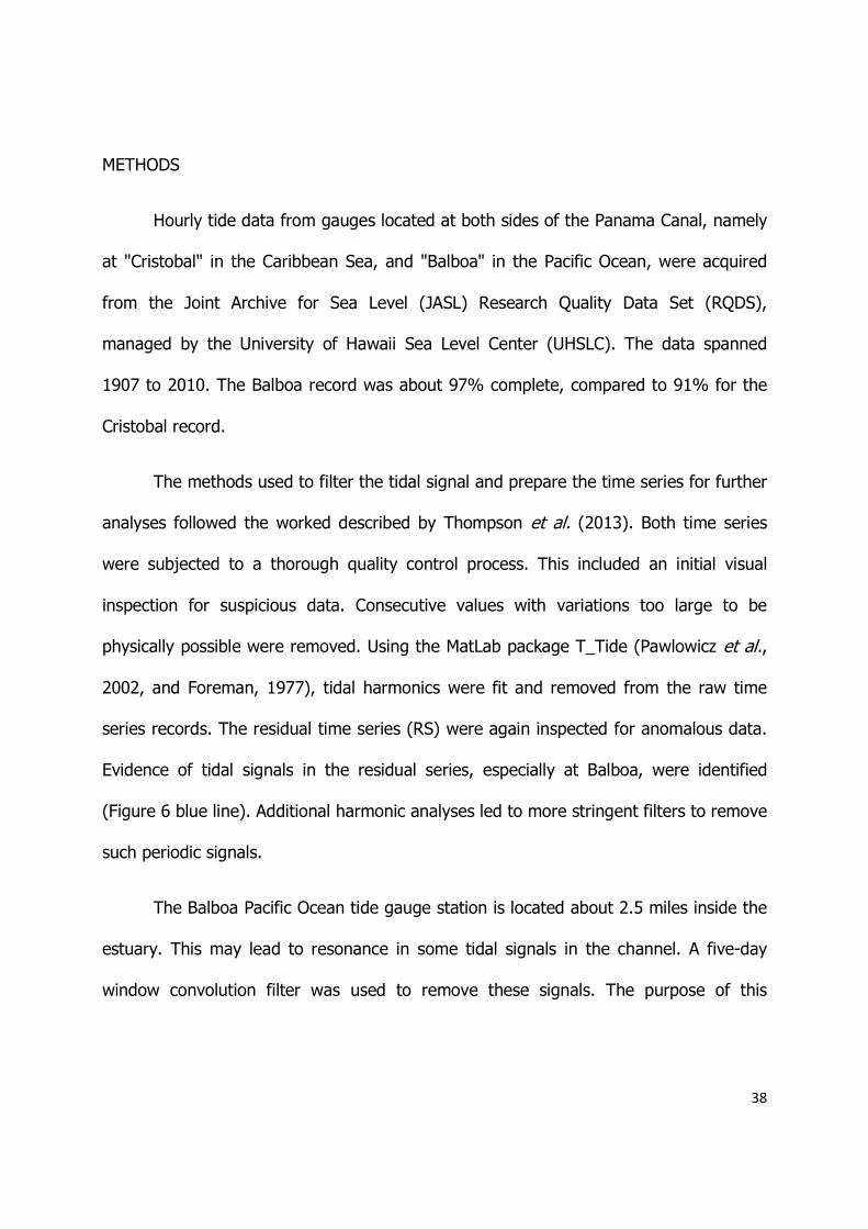
METHODS
Hourly tide data from gauges located at both sides of the Panama Canal, namely
at "Cristobal" in the Caribbean Sea, and "Balboa" in the Pacific Ocean, were acquired
from the Joint Archive for Sea Level (JASL) Research Quality Data Set (RQDS),
managed by the University of Hawaii Sea Level Center (UHSLC). The data spanned
1907 to 2010. The Balboa record was about 97% complete, compared to 91% for the
Cristobal record.
The methods used to filter the tidal signal and prepare the time series for further
analyses followed the worked described by Thompson et al. (2013). Both time series
were subjected to a thorough quality control process. This included an initial visual
inspection for suspicious data. Consecutive values with variations too large to be
physically possible were removed. Using the MatLab package T_Tide (Pawlowicz et al.,
2002, and Foreman, 1977), tidal harmonics were fit and removed from the raw time
series records. The residual time series (RS) were again inspected for anomalous data.
Evidence of tidal signals in the residual series, especially at Balboa, were identified
(Figure 6 blue line). Additional harmonic analyses led to more stringent filters to remove
such periodic signals.
The Balboa Pacific Ocean tide gauge station is located about 2.5 miles inside the
estuary. This may lead to resonance in some tidal signals in the channel. A five-day
window convolution filter was used to remove these signals. The purpose of this

39
convolution filter was to identify and remove remaining tidal signals. The resulting
signal is shown as a red line in Figure 6.
Figure 6. Balboa tide gauge sea level height series. Blue line shows tidal signal; red line corresponds to the filtered series.
An additional tidal fit was conducted on the raw data, using exclusively tidal
constituents with periods higher than one day. Visual inspection of the spectra
confirmed that only low frequency energy remained in this record, and that no
harmonics associated with tidal signals remained in the record (Figure 7). The residual
series were then sub-sampled twice a day. These results were used in subsequent
analyses.

Figure 7. Spectra of Balboa unfiltered time series (blueThe low frequency signal is preserved and high frequency energy is removed.
The 10% highest sea level
defined as the five day period encompassing the
reflect the effect that specific processes have on sea level
overestimation. The frequency of these events was
station, to evaluate whether the frequency of high sea level events ha
time or not. To compare stations, only the overlapping portions of the time series
records were considered.
The number of sea level maxima events was
determine if there was a seasonality in the number of peaks in sea level in each reco
A monthly sea level climatology was constructed by averaging all data available for
every month across years
virtual year). These monthly climatological values were then subtracted from every ye
in the time series to obtain a time series of anomalies.
Spectra of Balboa unfiltered time series (blue) and filtered time series (red). The low frequency signal is preserved and high frequency energy is removed.
The 10% highest sea level maxima events were identified. Each event was
five day period encompassing the highest sea level
reflect the effect that specific processes have on sea level
overestimation. The frequency of these events was then grouped by year for each
to evaluate whether the frequency of high sea level events ha
. To compare stations, only the overlapping portions of the time series
The number of sea level maxima events was then grouped by month
seasonality in the number of peaks in sea level in each reco
A monthly sea level climatology was constructed by averaging all data available for
across years to obtain 12 average values (i.e. one for each month of a
virtual year). These monthly climatological values were then subtracted from every ye
in the time series to obtain a time series of anomalies.
40
) and filtered time series (red). The low frequency signal is preserved and high frequency energy is removed.
were identified. Each event was
sea level measurements to
reflect the effect that specific processes have on sea level and to prevent
grouped by year for each
to evaluate whether the frequency of high sea level events had changed over
. To compare stations, only the overlapping portions of the time series
grouped by month, to
seasonality in the number of peaks in sea level in each record.
A monthly sea level climatology was constructed by averaging all data available for
one for each month of a
virtual year). These monthly climatological values were then subtracted from every year

41
The low-frequency sea level records obtained were compared to environmental
parameters including wind speed (u and v components), atmospheric pressure, and
synoptic sea height anomalies derived from satellites to help explain particular events.
Anomalies were also computed for each environmental dataset by subtracting a
climatology from the corresponding time series. The comparisons with sea level were
conducted in anomaly space.
Specifically, wind and atmospheric pressure data were extracted from the NCEP
reanalysis (NOAA Earth System Research Laboratory's Physical Science Division;
http://www.esrl.noaa.gov/psd/; see Kalnay et al., 1996). The resolution of these
gridded data is 210 km, sampled every 6 hours starting in 1948. The closest grid points
to Cristobal and Balboa were selected and sub-sampled to match the twice-daily
frequency of the sea level anomaly time series derived from tide gauges.
Steric sea level changes were calculated using the sea water state equation
(Millero et al., 1980, UNESCO, 1981), using seasonal salinity profiles obtained from the
NOAA National Oceanographic Data Center and satellite-derived monthly sea surface
temperature (SST) from Pathfinder Version 5.2 (PFV5.2; Casey et al., 2010). The
PFV5.2 were available for the period 1982-2012 at a spatial resolution of 4 km. Changes
in density were primarily caused by changes in the temperature, and these were
converted into changes in the height of the water column. The steric height record was
compared to the monthly average sea level anomaly time series obtained from the tide
gauge data.

42
All correlation analyses followed the work done by Davis (1976, 1977) to
determine the adequate number of degrees of freedom and Sciremammano (1979) to
calculate the p-values in order to account for the dependence between consecutive
values in any given time series, which is not accounted for in the standard correlation
(Sciremammano, 1979).
To determine if the events identified from the tide gauge observations were due
to local or to broader geographic scale processes, we compared satellite-derived sea
surface height anomaly series from a location close to each Cristobal and Balboa to the
filtered sea level records derived from the tide gauge data. The altimeter products were
obtained from the Centre National d'Etudes Spatieles-Archiving, Validation and
Interpretation of Satellite Oceanographic data (CNES-AVISO;
http://www.aviso.altimetry.fr/duacs/). We also explored any possible relationship
between the Multivariate ENSO Index (i.e. the MEI based in Wolter and Timlin, 1993)
and sea level. MEI data starting in 1950 were available from the National Oceanic and
Atmospheric Administration/Oceanic Atmospheric Research/Earth System Research
Laboratory/Physical Sciences Division NOAA/OAR/ESRL PSD (http: //www. esrl.noaa.
gov/psd/). Additionally, a comparison of El Niño historical record (spanning from 1907-
2010) and Balboa sea level record was done to further test any relationship between
the two series. A randomization test (1000 iterations) was done in order to determine if
the percentage of events that occurred during El Niño years followed a random
distribution or are in fact correlated. Only those years with counts higher than 3
standard deviations (rounded to 12 events) were considered for this analysis.

43
RESULTS
Monthly counts of non-tidal sea level maxima showed a seasonal signal, with
peaks in October for Cristobal and June/October for Balboa. The frequency distribution
shows averages of 7.30 +/- 4.14 events per year at Balboa (Figure 8a) and 7.29 +/-
3.74 events per year at Cristobal (Figure 8b).
a.
b.
Figure 8. Frequency of non-tidal yearly grouped sea level events from Balboa (a.) and Cristobal (b.) stations.
There was no significant trend in the number of events over the span of the
entire time-series at Balboa. However, there was an increase in events in Balboa
between 1981 and 1982 to almost 20 events each year, and again in 1997 (17 events)
and 2002 (14 events). While these corresponded to positive values of the Multivariate
44
ENSO Index, not all years with positive MEI showed an anomalous number of events at
Balboa. Cristobal, on the other hand, showed fewer anomalous high sea level events
after 1990.
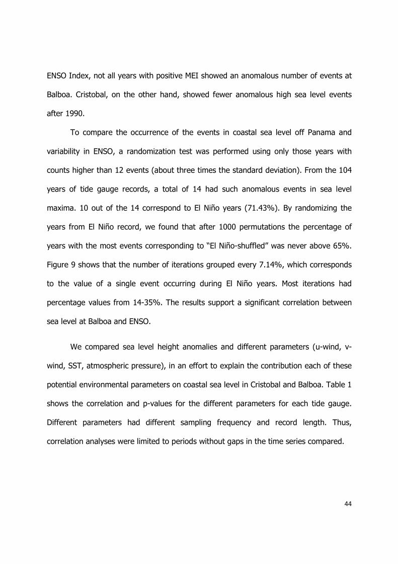
To compare the occurrence of the events in coastal sea level off Panama and
variability in ENSO, a randomization test was performed using only those years with
counts higher than 12 events (about three times the standard deviation). From the 104
years of tide gauge records, a total of 14 had such anomalous events in sea level
maxima. 10 out of the 14 correspond to El Niño years (71.43%). By randomizing the
years from El Niño record, we found that after 1000 permutations the percentage of
years with the most events corresponding to “El Niño-shuffled” was never above 65%.
Figure 9 shows that the number of iterations grouped every 7.14%, which corresponds
to the value of a single event occurring during El Niño years. Most iterations had
percentage values from 14-35%. The results support a significant correlation between
sea level at Balboa and ENSO.
We compared sea level height anomalies and different parameters (u-wind, v-
wind, SST, atmospheric pressure), in an effort to explain the contribution each of these
potential environmental parameters on coastal sea level in Cristobal and Balboa. Table 1
shows the correlation and p-values for the different parameters for each tide gauge.
Different parameters had different sampling frequency and record length. Thus,
correlation analyses were limited to periods without gaps in the time series compared.

45
Figure 9. Frequency histogram for the randomization test between sea level maxima events at Balboa and El Niño years. Percentage of events occurring during “El Niño-shuffled” are grouped in bins every 7.14% equivalent to 1/14th of the events coinciding with ENSO.
The analysis shows that low-frequency signals in sea level at Cristobal had no
particular relationship to winds. Balboa showed a slight positive correlation between the
zonal wind (East-West) component and sea level anomaly: up to ~20% of the
variability in sea level could be attributed to changes in this wind component. However,
this correlation was only statistically significant (p-value <0.05) for part of the record.
No correlation (<5%) was identified with the v-wind component. Changes in
atmospheric pressure had no measurable effect on sea level (r<0.05) at either location.
The variability in sea level seemed to follow changes in sea surface temperature
at Balboa but not at Cristobal. A correlation coefficient of up to 0.35 suggested that
steric height changes were significant in defining local sea level at Balboa. However due
to the length of the record, this correlation might be spurious. The dependence of
0 10 20 30 40 50 60 70 800
50
100
150
200
250
300
350Frequency histogram for the randomization test
Percentage of events occuring during El Niño years
Num
ber
of
itera
tions
Percentage of years ofmaxima events that
correspond to El Niñoyears: 71.43%

46
consecutive values in time series reduces the number of independent points in such
series (Sciremammano, 1979), therefore, there might not be enough data to validate
the correlation mentioned above. Lag-correlations were calculated, but none of the
parameters showed any evidence of lag correlation with sea level changes.
To examine the nature of the events at Balboa, we observed their duration and
geographical extent using the satellite-derived SSH fields. This analysis was intended to
determine whether events were locally generated or if they were a response to a larger-
scale process such as the El Niño Southern Oscillation (ENSO) or La Niña events.
Table 9. Correlation coefficients for a comparison between different environmental parameters and the Balboa and Cristobal sea level anomalies. Bolded values represent statistically significant correlation values (95% confidence level). *Sea Surface Height computed from SST data.
v-wind u-wind Atm. Pressure Steric
SSH(SST)*
r p-val. r p-val. R p-val. r p-val.
Balboa 0.039 0.029 0.153 0.043 -0.053 0.042 0.166 0.226
0.056 0.056 0.198 0.087 -0.038 0.077 0.204 0.176
0.031 0.043 0.143 0.068 -0.004 0.060 0.354 0.286
0.011 0.078 0.171 0.096 0.009 0.092
Cristobal -0.042 0.027 -0.038 0.037 0.018 0.035 -0.072 0.140
-0.010 0.041 -0.040 0.052 0.021 0.050 -0.120 0.206
-0.383 0.450 -0.147 0.350 0.117 0.424
Balboa station showed significant coherence with variability in sea surface height
variability observed over very large spatial scales in the tropical Pacific. For example, in
1994 we detected sea level anomalies synchronous with a process that affected the
entire tropical Pacific Ocean (Figure 10). Satellite altimeter data showed a positive
anomaly in the central Pacific in August, which reached up to 28 cm and extended from
170° W to 130° W and 5° S to 9.5° N. This feature propagated toward the East and
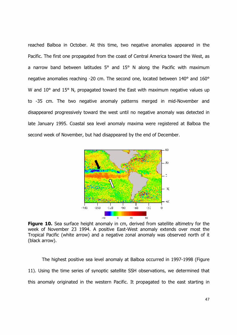
reached Balboa in October. At this time, two negative anomalies appeared in the
Pacific. The first one propagated from the coast of Central America toward the West
a narrow band between latitudes 5° and 15° N along the Pacific with maximum
negative anomalies reaching
W and 10° and 15° N, propagated to
to -35 cm. The two negative anomaly patterns merg
disappeared progressively toward the west until no negative anomaly was detected in
late January 1995. Coastal sea level anomaly maxima
second week of November, but
Figure 10. Sea surface height anomalyweek of November 23 1994. A positive Tropical Pacific (white arrow) and a negative (black arrow).
The highest positive sea level anomaly at Balboa occurred in 1997
11). Using the time series of synoptic satellite SSH observations, we
this anomaly originated in the western Pacific. It propagated to the east starting in
reached Balboa in October. At this time, two negative anomalies appeared in the
ropagated from the coast of Central America toward the West
a narrow band between latitudes 5° and 15° N along the Pacific with maximum
reaching -20 cm. The second one, located between 140° and 160°
propagated toward the East with maximum negative values up
35 cm. The two negative anomaly patterns merged in mid
progressively toward the west until no negative anomaly was detected in
late January 1995. Coastal sea level anomaly maxima were registered at Balboa
, but had disappeared by the end of December.
ea surface height anomaly in cm, derived from satellite altimetry for the week of November 23 1994. A positive East-West anomaly extends over mosTropical Pacific (white arrow) and a negative zonal anomaly was observed
The highest positive sea level anomaly at Balboa occurred in 1997
11). Using the time series of synoptic satellite SSH observations, we
this anomaly originated in the western Pacific. It propagated to the east starting in
47
reached Balboa in October. At this time, two negative anomalies appeared in the
ropagated from the coast of Central America toward the West, as
a narrow band between latitudes 5° and 15° N along the Pacific with maximum
located between 140° and 160°
ward the East with maximum negative values up
ed in mid-November and
progressively toward the west until no negative anomaly was detected in
re registered at Balboa the
had disappeared by the end of December.
derived from satellite altimetry for the
anomaly extends over most the was observed north of it
The highest positive sea level anomaly at Balboa occurred in 1997-1998 (Figure
11). Using the time series of synoptic satellite SSH observations, we determined that
this anomaly originated in the western Pacific. It propagated to the east starting in

March 1997, and reached the eastern pacific about 6 weeks later. It was detected at
Balboa the first week of May. The largest anomaly was detected the wee
3, 1997. This particular event lasted until mid
strong El Niño event of 1997
Figure 11. Sea surface height anomalyweek of December 3 1997. A large positive anomaly extendTropical Pacific (large arrow) and and south along the coast in the
We observed another e
2002. This event was not detected in the altimetry observations
and spatial resolution of the altimetry data
lived events observed in the ti
related to larger, synoptic signals.
Visual inspection of the altimetry data shows a
tropical Pacific in July 2002. This feature propagated to the East, and reached Balboa
March 1997, and reached the eastern pacific about 6 weeks later. It was detected at
Balboa the first week of May. The largest anomaly was detected the wee
3, 1997. This particular event lasted until mid-January 1998. This corresponded to the
strong El Niño event of 1997-1998 that lasted almost eight months.
ea surface height anomaly in cm, derived from satellite altimetry for the week of December 3 1997. A large positive anomaly extended over most Tropical Pacific (large arrow) and appeared to propagate over time
along the coast in the eastern Pacific (small arrows).
We observed another event in Balboa that lasted about two weeks in January
2002. This event was not detected in the altimetry observations because
and spatial resolution of the altimetry data are not fine enough. Several other short
lived events observed in the tide gauge record in the Panama Bight were not
related to larger, synoptic signals.
Visual inspection of the altimetry data shows another large SSH event in the
tropical Pacific in July 2002. This feature propagated to the East, and reached Balboa
48
March 1997, and reached the eastern pacific about 6 weeks later. It was detected at
Balboa the first week of May. The largest anomaly was detected the week of December
January 1998. This corresponded to the
derived from satellite altimetry for the
over most of the eastern over time towards the north
vent in Balboa that lasted about two weeks in January
because the temporal
not fine enough. Several other short-
ight were not clearly
large SSH event in the
tropical Pacific in July 2002. This feature propagated to the East, and reached Balboa
49
after 7 weeks. This time frame corresponded to a gap in the tide gauge data and it was
not possible to examine the relationship to coastal sea level off Panama.
Visual inspection of the satellite altimetry data for the western Caribbean Sea,
and particularly off the coast of Panama by the Cristobal station, showed a pattern of
positive and negative anomalies related to the presence of westward-moving cyclonic
and anti-cyclonic eddies in the southwestern Caribbean. However, there was no
significant statistical correlation between the satellite altimetry records and the Cristobal
sea level time series. It is possible that the spatial resolution of the satellite data is not
sufficient to capture some of the details of the sea surface elevation variability in this
area of the Gulf of Darien.
DISCUSSION
Sea level varies as a result of different and complex forcing components of the
climate system, including direct and indirect forcing (Cazenave and LLovel, 2010). A
detailed examination of the century-long sea level records at the Cristobal and Balboa
tide gauges off Panama shows that it is difficult to find a clear link between major
forcing parameters and coastal sea level, particularly at Cristobal in the Caribbean Sea.
Neither the Balboa nor the Cristobal time series show long-term trend in anomalies.
Some of the largest low-frequency sea level changes at Balboa were related to
large-scale changes in the tropical Pacific Ocean. Particularly, more than 70% of the
years with higher counts of sea level maxima events occurred during El Niño years

50
showing a direct relationship between sea level maxima and ENSO. While there is no
statistically significant correlation between sea level at Balboa and SST or the intensity
of the zonal wind, visual examination of their series suggests that there is some forcing
of specific sea level events, especially as observed synoptically using satellite altimeter
data. Sea level anomaly signals propagated to the east, and reached the coast in the
1994 and 1997-1998 El Niño events. These are equatorial downwelling Kelvin waves
that move from the western Pacific warm pool to the eastern Pacific (McPhaden, 1999;
Kessler and McPhaden, 1995). These waves cause a deepening of the thermocline,
reducing the upwelling in the eastern Pacific, This generates a positive SST anomaly
(Boulanger and Menkes, 1995). This is usually a consequence of changes in the
intensity and strength of the trade winds in the central Pacific Ocean. Figure 6 shows
the result of signal propagating along the coast of North and South America as coastal
Kelvin waves.
We found no correlation with the north-south component of wind at Cristobal or
Balboa. A negative correlation was expected at Balboa because of the atmospheric
Panama Jet caused by strong winds channeled through the mountains of Panama from
the Caribbean, and which blowing from the North creates a strong and persistent cold
water signal in the Pacific despite being the weaker of the three Jets in the region
(Quiros et al., 2007; Lluch-Cota et al., 2007; Chelton et al., 2000; Gaxiola-Castro and
Muller-Karger, 1998). It is possible that the duration and intensity of the Panama Jet
generates a seasonal response in sea level that was filtered out in our pre-processing of
the coastal tide gauge data. Furthermore, multi-decadal variation of the winds in the
51
region does not explain the sea level variation detected. On the other hand, the
Panama Jet leads to marked changes in SST due to turbulent mixing and upwelling.
This signal is isolated to the area directly affected by high winds and dissipates rapidly
in space and in time (Liang et. al., 2009; Sun and Yu, 2006). There is no evidence of a
drop in sea level as consequence of the wind jets in the tide gauge data, despite the
wind-driven formation of eddies (Muller-Karger and Fuentes-Yaco, 2000). These eddies
are also evident in the altimetry data as lower SST and highest negative SSH anomalies
that also have been reported south to the path of the seasonal Panama Jet based on
satellite data. However these products exclude the coastal data (Rodriguez-Rubio et al.,
2003).
Our results show that Balboa sea level anomalies seem to be modulated by
changes in temperature and, in a minor way, by changes in zonal wind strength. There
is a clear correlation between sea level maxima at Balboa and ENSO events. In
contrast, variability in low-frequency sea level at Cristobal in the Caribbean Sea can not
be explained with the parameters examined.
REFERENCES
Barnett, T.P., 1984: The estimation of "global" sea level change: A problem of
uniqueness, J Geophys Res, 89(C5), 7980-7988,
doi:10.1029/JC089iC05p07980.

52
Beckley, B.D., F.G. Lemoine, S.B. Luthcke, R.D. Ray and N.P. Zelensky, 2007: A
reassessment of global and regional mean sea level trends from TOPEX and
Jason-1 altimetry based on revised reference frame and orbits, Geophys Res
Lett, 34, L14608, doi:10.1029/2007GL030002.
Boulanger, J. and C. Menkes, 1995: Propagation and reflection of long equatorial
waves in the Pacific Ocean during the 1992-1993 El Niño, J Geophys Res:
Oceans, 100(C12), 25041-25059, doi:10.1029/95JC02956
Casey, K.S., T.B. Brandon, P. Cornillon and R. Evans, 2010: The Past, Present and
Future of the AVHRR Pathfinder SST Program, Oceanography from Space:
Revisited, eds. V. Barale, J.F.R. Gower and L. Alberotanza, Springer. doi:
10.1007/978904818681516.
Cazanave, A. and W. Llovel, 2010: Contemporary Sea Level Rise, Annual Review of
Marine Science, 2, 145-173, doi:10.1146/annurev-marine-120308-081105.
Cazenave, A., A. Lombard and W. Llovel, 2008: Present-day sea level rise: A synthesis,
Comptes Rendus Geoscience, 340(11), 761-770.
doi:10.1016/j.crte.2008.07.008.
Cazenave, A., K. Dominh, S. Guinehut, E. Berthier, W. Llovel, G. Ramillien, M. Ablain
and G. Larnicol, 2009: Sea level budget over 2003–2008: A reevaluation from
GRACE space gravimetry, satellite altimetry and Argo, Glob Planet Change,
doi:10.1016/j.gloplacha.2008.10.004

53
Chelton, D.B., F.J. Wentz, R.A. de Szoeke and M.G. Schlax, 2000: Satellite microwave
SST observations of transequatorial tropical instability waves, Geophys Res Lett
27(9), 1239-1242. doi: 10.1029/1999GL011047.
Church, J.A. and N.J. White, 2011: Sea-level rise from the late 19th to the early 21st
Century, Surveys in Geophysics, 32(4-5), 585-602, doi:10.1007/s10712-011-
9119-1.
Church, J.A. and N.J. White, 2006: A 20th century acceleration in global sea-level rise,
Geophys Res Lett, 33, L01602, doi:10.1029/2005GL024826.
CNES-AVISO (Centre National d'Etudes Spatieles-Archiving, Validation and
Interpretation of Satellite Oceanographic data) available at
www.aviso.altimetry.fr/duacs/
Davis, R.E., 1976: Predictability of sea surface temperature and sea level pressure
anomalies of the North Pacific, J Phys Oceanogr, 6, 249-266.
Davis, R.E., 1977: Techniques for statistical analysis and prediction of geophysical fluid
systems, Geophys Astrophys Fluid Dyn 8, 245-277.
Fairbridge, R.W. and O.A. Krebs, 1962: Sea Level and the Southern Oscillation. Geophys
J Roy Astr S 6, 532-545, doi: 10.1111/j.1365-246X.1962.tb02999.x.
Foreman, M.G., 1977: Manual for tidal heights analysis and prediction. Pacific Marine
Science Report 77-10, Institute of Ocean Sciences, Patricia Bay, Sidney, BC,
97pp.
Gaxiola-Castro, G. and F. E. Muller-Karger, 1998: Seasonal phytoplankton pigment
variability in the Eastern Tropical Pacific Ocean as determined by CZCS imagery.
54
In: Remote Sensing Tropical Pacific Ocean by Satellites. R. A. Brown (Editor).
PORSEC, 1998. Earth Ocean and Space Pty. Ltd. 271-277/
Holgate, S.J. and P.L. Woodworth, 2004: Evidence for enhanced coastal sea level rise
during the 1990s, Geophys Res Lett, 31(7), doi: 10.1029/2004GL019626.
Jevrejeva, S., A. Grinsted, J. Moore and S. Holgate, 2006: Nonlinear trends and
multiyear cycles in sea level records, J Geophys Res, 111, C09012,
doi:10.1029/2005JC003229.
Jevrejeva, S., J.C. Moore, A. Grinsted, A.P. Matthews and G. Spada, 2014: Trends and
acceleration in global and regional sea levels since 1807, Global Planet Change,
113, 11-22, doi:10.1016/j.gloplacha.2013.12.004.
Kalnay, E., M. Kanamitsu, R. Kistler, W. Collins, D. Deaven, L. Gandin, M. Iredell, S.
Saha, G. White, J. Woolleen, Y. Zhu, M. Chelliah, W. Ebisuzaki, W. Higgins, J
Janowiak, K.C. Mo, C. Ropelewski, J. Wang, A. Leetmaa, R. Reynolds, Roy Jenne
and D. Joseph, 1996: The NCEP/NCAR 40-year Reanalysis, Project Bull Amer
Meteor Soc, 77, 437–472.
Kaser, G., J.G. Cogley, M.B. Dyurgerov, M.F. Meier and A. Ohmura, 2006: Mass balance
of glaciers and ice caps: Consensus estimates for 1961-2004, Geophys Res Lett,
33(19), L19501, doi:10.1029/2006GL027511.
Kessler, W.S. and M.J. McPhaden, 1995: Oceanic equatorial waves and the 1991-93 El
Niño, J Climatol, 8, 1757-1774.

55
Leuliette, E.W. and L. Miller, 2009: Closing the sea level rise budget with altimetry,
Argo, and GRACE, Geophys Res Lett, 36(4), L04608,
doi:10.1029/2008GL036010.
Levitus, S., J. Antonov and T. Boyer, 2005: Warming of the world ocean, 1955-2003,
Geophys Res Lett, 32, L02604, doi:10.1029/2004GL021592.
Liang, J.-H., J.C. McWilliams and N. Gruber, 2009: High-frequency response of the
ocean to mountain gap winds in the northeastern tropical Pacific, J Geophys Res,
114, C12005, doi:10.1029/2009JC005370.
Lluch-Cota S.E., S. Alvarez-Borrego, E. Santamaría-del-Angel, F.E. Muller-Karger and S.
Hernández-Vázquez, 1997: El Golfo de Tehuantepec y áreas adyacentes:
Variación espacio-temporal de pigmentos fotosinteticos derivados de satelite.
Cienc Mar, 23(3):329-340.
McPhaden, M.J., 1999: Genesis and Evolution of the 1997-98 El Niño, Science, 283,
950-954, doi: 10.1126/science.283.5404.950.
Millero, F.J., C.-T. Chen, A. Bradshaw and K. Schleicher, 1980: A new high-pressure
equation of state for seawater, Deep-sea Res, 27A, 255-264.
Muller-Karger, F.E. and C. Fuentes-Yaco, 2000: Characteristics of wind-generated rings
in the eastern tropical Pacific Ocean, J Geophys Res, 105(C1), 1271-1284, doi:
10.1029/1999JC900257.
Nerem, R.S., D.P. Chambers, C. Choe and G.T. Mitchum, 2010: Estimating Mean Sea
Level Change from the TOPEX and Jason Altimeter Missions, Mar Geod, 33, 435-
443, doi:10.1080/01490419.2010.491031.
56
Pawlowicz, R., B. Beardsley and S. Lentz, 2002: Classical tidal harmonic analysis
including error estimates in MATLAB using T_TIDE, Computers and Geosciences,
28, 929-937, doi:10.1016/S0098-3004(02)00013-4.
Quiros, G. and F. E. Muller-Karger, 1997: Dynamics of satellite-viewed rings near the
Costa Rica Thermal Dome, Rev Geofis, Instituto Panamericano de Geografia e
Historia, 46 Enero-Junio 1997.
Rahmstorf, S., 2007: A Semi-Empirical Approach to Projecting Future Sea-Level Rise,
Science, 315, 368-370, doi:10.1126/science.1135456.
Rodriguez-Rubio, E., W. Schneider and R. Abarca del Rio, 2003: On the seasonal
circulation within the Panama Bight derived from satellite observations of wind,
altimetry and sea surface temperature, Geophys Res Lett, 30(7), 1410,
doi:10.1029/2002GL016794.
Sciremammano, F. 1979: A Suggestion for the Presentation of Correlations and Their
Significance Levels, J Phys Ocean, 9(6), 1273-1276, doi:10.1175/1520-
0485(1979)009<1273:ASFTPO>2.0CO;2.
Small, C. and R.J. Nichols, 2003: A Global Analysis of Human Settlement in Coastal
Zones, J Coast Res, 19(3), 584-599.
Sun, F. and J.-Y. Yu, 2006: Impacts of Central America gap winds on the SST annual
cycle in the eastern Pacific warm pool, Geophys Res Lett, 33, L06710,
doi:10.1029/2005GL024700.
Thompson, P.R., G.T. Mitchum, C. Vonesch and J. Li, 2013: Variability of Winter
Storminess in the Eastern United States during the Twentieth Century from Tide

57
Gauges, J Climate, 26, 9713-9726, doi:http://dx.doi.org/10.1175.JCLI-D12-
00561.1
Trenberth, K.E., 1997: The Definition of El Niño, Bull Amer Met Soc, 78, 2771-2777.
UNESCO, 1981: Background papers and supporting data on the International Equation
of State of Sea-water 1980, UNESCO R M, 38, UNESCO, Paris.
Vermeer, M. and S. Rahmstorf, 2009: Global sea level linked to global temperature.
Proc Natl Acad Sci, 106, 21527-21532, doi:10.1073/pnas.0907765106.
Wolter, K. and M.S. Timlin, 1993: Monitoring ENSO in COADS with a seasonally
adjusted principal component index. Proc. of the 17th Climate Diagnostics
Workshop, Norman, OK, NOAA/NMC/CAC, NSSL, Oklahoma Clim Survey, CIMMS
and the School of Meteor, Univ of Oklahoma, 52-57.

58
SUMMARY
Several misconceptions were identified in the first chapter of the present study both
before and after the curriculum unit (CU) was implemented among 7th and 8th grade
students. Responses from the later reflected, in general, a better understanding of the
concepts pos-CU including more accurate concepts and scientific vocabulary and theory
taught as part of the lessons. Climate change, climate and temperature were used
interchangeably. Sea level was often defined as either ocean’s depth or height but
without including a land reference. These findings are similar to previous studies that
include complex concepts such as global warming and green-house effect. Evidence of
misconceptions has been found in different group ages and in most cases those
misconceptions have been retained. No study previously done with 7th or 8th grade
students report the level of improvement herein obtained among the later. However
new misconceptions were reported pos-CU perhaps due to the short duration of the
lessons. The use of scientific data was not guarantee of an understanding of these
Earth system processes which highlights the importance of a continuous and
comprehensive effort in order to improve the level of understanding and to build the
correct conceptual framework within the students. Relating these processes to students’
personal life and creating a clear link between them could create the proper
environment for a better and more fructuous learning experience. We use Piaget’s

59
theory of children’s cognitive development as a way to explain the differences we report
between 7th and 8th grade students. He states that around age 11 or 12 children
transition into a more mature developmental stage in which they are capable of
understanding complex concepts including several variables as climate change and sea
level rise are. On the other hand these differences could be due solely to the fact that
8th grade students have had one more year of experiencing some of the concepts
therefore are more familiarized with complex thinking.
Time series analysis of sea level at Balboa (Pacific ocean) and Cristobal (Caribbean sea)
at both sides of the Panama canal showed the inherent difficulties to determine the
parameter or parameters that control sea level at these coastal locations. Neither time
series show an increase in the number of anomalous events along the length of the
record. More than 70% of the sea level maxima non-tidal events at Balboa occurred
during El Niño years, thus sea level at this location is modulated by large-scale
processes that affect the entire oceanic basin. The correlation found with the wind
zonal component and the apparent correlation with temperature is also explained by
the ENSO effect on sea level. Changes in the intensity (weakening) of the trade winds
(which have a strong zonal component) create a series of events that ultimately (in
most cases) generate a shift of the thermocline in the Pacific Ocean basin. Anomalous
high sea surface temperatures occur in the Eastern Pacific, which have a steric effect on
sea level hence the positive correlation between these parameters (cf.). Meridional wind
component show no effect on sea level at Balboa despite the seasonal presence of the
Panama Jet caused by the funneling of strong winds from the Caribbean through the

60
mountains of Panama. Altimetry imagery was used to visually confirm the correlation
between ENSO and anomalies from tide gauge at Balboa. Most events had a basin-wide
distribution and are explained by that correlation however some are locally generated
and probably caused by complex interactions that are difficult to resolve with the data
available.

61
APPENDIX A
CURRICULUM UNIT
Activities and instructions developed as part of the lesson plan implemented during
2012 and 2013 with 7th and 8th grade students.
LESSON 1: CLIMATE VS. WEATHER (1-2 periods)
Activities: Melting ice experiment, Global Warming reading
Students start their melting ice experiment with ice floating in their models and
the teacher sets the model with ice sitting outside the water. Students hypothesize
what will happen to the water level after the ice melts. While the ice is melting and
between measurements teacher leads a discussion to define weather, climate and
climate change in students' own words. Once all the ice melts students discuss their
results and try to explain what happened. Two short video clips are presented to
compare melting ice floating with melting ice sitting on a structure outside the water.
Students conclude based upon their results and the videos and the parallel to real life is
explained: only melting ice on land will cause sea level to rise.

62
Students take turns to read Global Warming by Holli Riebeek available at
http://earthobservatory.nasa.gov/Features/GlobalWarming/. Students discuss the
difference between global warming and climate change and the consequences of
climate change. Special attention is given to the consequences more relevant to the
State of Florida specially sea level rise.
LESSON 2: GLACIAL VS. INTERGLACIAL; ANCIENT SEA LEVEL CHANGE (2 periods)
Activities: North America map
The lesson starts with the two video clips from the previous lesson as a way to
reinforce the effect of melting ice on land compared to floating ice. Teacher presents
scientific evidence to past climate and sea level changes (glacial and interglacial
periods). Students develop the North America map activity. Using the template provided
(North America map) students must draw the coast line and ice cover at different
moments in the geological earth's history (e.g. last glacial maximum 18 kya, Eocene
about 50 mya). This activity will help students to recognize how sea level has changed
in the past, how it relates to ice coverage on land. Images of different periods on earth
history are available at Paleomap project: http://scotese.com/earth.htm. The North
America map is available at: http://www.eduplace.com/ss/maps/pdf/n_america_nl.pdf.
For the second part of this lesson the teacher presents a plot including
temperature change, ice coverage and CO2 concentration for the past 450 kya.
Students will observe the plot and discuss the observations. The saw tooth pattern is

63
discussed and the effect temperature has on ice coverage is explained. The relation
between CO2 concentration to temperature and ice coverage is also explained.
Finally a plot including current levels of CO2 are discussed in relation to recorded
glacial and interglacial values and sea level rise from last glacial maximum is explained
as a consequence of the rapid melting of ice sheets.
LESSON 3: SEA LEVEL AND SEA LEVEL RISE (2 periods)
Activities: What changes sea level?, thermal expansion.
For this lesson, students are introduced to the definitions of sea level and mean
sea level. The importance of a reference point in land is highlighted. Basic concepts
related to tides are explained. The interaction between the Moon, Sun and Earth and its
effect on the tides are illustrated using simple models (e.g. balls of different size). The
level of detail in this lesson will depend on previous knowledge and understanding of
the concepts. Teacher provides sea level definition in terms of high and low tides.
Using a clear tank half-full of water, cups, spraying sprinkler bottle, fan, and
other simple items, students take turns to mimic different processes or natural forces
that affect sea level (e.g. waves, wind, precipitation, etc). Teacher must encourage
most students to participate. A clear bowl can serve as a second model, which can be
used to simulate currents and will provide a clear image.

64
The second period will start by introducing the concept of sea level rise linking it
to previous lessons. Two plots are discussed in this part of the lesson, CO2
concentration from the last thousand years and sea level change from the last 120
years. The two main causes of sea level rise are discussed, namely, ice melting (from
glaciers and ice sheets) and thermal expansion.
For the thermal expansion activity, six students are selected and used to explain
thermal expansion, each one become a water molecule and by moving them away or
approaching to each other the concepts of volume and density as a function of
temperature are easily demonstrated.
The final part of the lesson consists on teaching the different equipments used to
measure sea level. A description of the principle used to measure sea level in tide
gauges is explained with the help of a yardstick; emphasizing the need of nearby land
as a reference point. It is also briefly explained the use of satellite to measure sea level.
The differences, weaknesses and benefits of each method are highlighted.
LESSON 4: FUTURE SEA LEVEL (3-4 periods)
Activities: Tide gauge data analysis.
For this final lesson one tide gauge is used as example. Teacher presents a plot
of sea level vs. time and students visually inspect it to identify trends, patterns,
minimum and maximum values. The trend line should be included in the plot for the

65
students to easily identify it. In order to better illustrate the rise in sea level other line is
included in the plot. This line corresponds to the trend if sea level was not rising. The
contrast between the two lines should be evident even for those students that might
have had problems identifying the rising trend. This plots should serve as proof that sea
level has been rising in the last few decades and students should be able to infer that it
is very likely that sea level will continue to rise in the future. Teacher explains the
difficulties that projecting sea level into the future presents. A plot with different sea
level rise projections will be discussed; it is important to help students understand the
uncertainty and the limitations of these projections. It is also important to prevent
students from feeling afraid or hopeless but to encourage them to become part of the
solution.
For the second part of the lesson, students working in pairs will be assigned a US
tide gauge station, monthly data will be already prepared for students to use. Each pair
must use their dataset and plot sea level vs. time and include the trend. Students must
analyze their stations, observing the patterns, maximum and minimum values, and how
sea level changes through time. Using the trend it is possible to determine the rate of
change of sea level. Students will be lead to obtain this information.
Finally each pair will present their results and conclusions to their peers, special
attention will be given to the length of the record, maximum and minimum values,
patterns, trend (is it going up, down or is the same) how fast is changing and why?. At
the end of the presentations the teacher will lead a discussion and the class will

66
conclude based on the data whether sea level is rising or not and what is going to
happen to sea level in the future if things continue to be the same.
FIELD TRIP: VISIT TO THE COLLEGE OF MARINE SCIENCE (half day)
After students have completed the course, a visit to the College of Marine
Science USF is scheduled. The visit consists in three stations: Center for Ocean
Technology, Remote Sensing and Tide gauge and other instruments. Each station
provides information on technology used by scientists to study the ocean including the
study of sea level. Finally students will participate in a session of questions and answers
with an expert on sea level science, a researcher that has study the subject for the last
few decades. This experience will allow students to interact with different scientists and
technology that will contribute to a better understanding of the subject.
RESOURCES
Melting Ice Record Sheet
http://www.teachingboxes.org/seaLevel/lessons/lesson2_activity2.jsp
Melting Ice Videos
http://oceandrilling.coe.tamu.edu/curriculum/Sea_Level/Ice_Volume/activity.html
Global Warming Reading

67
http://earthobservatory.nasa.gov/Features/GlobalWarming/
North America Map
http://www.eduplace.com/ss/maps/pdf/n_america_nl.pdf
Paleomap Project:
http://scotese.com/earth.htm
Tide Gauge Data
http://www.psmsl.org
68
APPENDIX B
RUBRICS FOR THE 2013 QUESTIONAIRE
Rubrics constructed for the items in the 2013 test including individual rubrics for
written, illustration and combined responses (written + drawing).
1. WHAT IS SEA LEVEL? EXPLAIN AND ILLUSTRATE.
Written
0: No answer, incorrect answer with no land reference or tautology (i.e. "the level of
the sea")
1: Sea level defined as the surface of the water or the level of the water
2: Incorrect answer that includes land reference
3: Sea level defined as the height of the sea or the ocean depth (incorrect answer)
4: Correct answer, sea level defined as the surface of the sea in reference to land (i.e.
"where the water meets the land" is an accepted definition)
69
Illustration
0: No illustration or the illustration does not define sea level
1: Sea level is the surface of the water, no land reference included
2: Sea level is the height or depth of the ocean, no land reference included
3: Sea level is the height or depth of the ocean, land reference is included or is
illustrated as the sea surface including above and below sea level references
4: Illustration includes land reference and a properly shows sea level
Combined
0: Incorrect illustration and/or contradicts the written response
1: Both incorrect
2: Correct illustration, incorrect response
3: Illustration and response are correct
4: Illustration and response are correct, illustration provides additional information that
enhances the response
70
2. IS SEA LEVEL THE SAME EVERYWHERE? EXPLAIN AND ILLUSTRATE.
Same as question number 3.
3.IS SEA LEVEL THE SAME ALL THE TIME? EXPLAIN AND ILLUSTRATE.
Written
0: No answer or incorrect answer
1: Yes it is the same (no explanation included)
2: No it is different (no reason or incorrect reason)
3: No is not the same (at least one correct reason)
4: No it is different (two or more correct reasons)
Illustration
0: No illustration or the illustration does not show sea level
1: Illustration of sea level being even
2: Illustration of sea level being different but the concept is not completely correct
3: Correct illustration of sea level being different

71
Combined
0: Incorrect illustration and/or contradicts the written response
1: Both incorrect
2: Correct illustration, incorrect response
3: Illustration and response are correct
4: Illustration and response are correct, illustration provides additional information that
enhances the response
72
APPENDIX C
INSTITUTIONAL REVIEW BOARD APPROVAL LETTERS
The University of South Florida Institutional Review Board produced two letters of
approval that applied to the current research.
October 15, 2010
Jeffrey Ryan
Geology
Department of Geology, Univ. South Florida
4202 East Fowler Ave., SCA 528
RE: Expedited Approval for Initial Review
IRB#: Pro00002139
Title: Coastal Areas Climate Change Education (CACCE) Partnership
73
Dear Jeffrey Ryan:
On 10/14/2010 the Institutional Review Board (IRB) reviewed and APPROVED the above referenced protocol. Please note that your approval for this study will expire on 10-
14-11.
Approved Items: Protocol Document(s):
CACCE Partnership Study Protocol 8/31/2010 10:48 AM 0.01
Consent/Assent Document(s):
Adult Interview & Focus Group Informed
Consent.pdf
10/15/2010 8:31
AM 0.01
Parental Informed Consent.pdf 10/15/2010 8:31
AM
0.01
Waiver of ICD granted for 1. the Adult Online Survey recruitment script, 2. the Adult Written Survey recruitment script, and 3. Child Assent script for surveys (done in Hillsborough Public Schools - ages 9-18)

74
Study involves children and falls under 45 CFR 46.404: Research not involving more than minimal risk.
It was the determination of the IRB that your study qualified for expedited review which includes activities that (1) present no more than minimal risk to human subjects, and
(2) involve only procedures listed in one or more of the categories outlined below. The
IRB may review research through the expedited review procedure authorized by
45CFR46.110 and 21 CFR 56.110. The research proposed in this study is categorized
under the following expedited review category:
(6) Collection of data from voice, video, digital, or image recordings made for research purposes.
(7) Research on individual or group characteristics or behavior (including, but not limited to, research on perception, cognition, motivation, identity, language, communication, cultural beliefs or practices, and social behavior) or research employing survey,
interview, oral history, focus group, program evaluation, human factors evaluation, or quality assurance methodologies.
Please note, the informed consent/assent documents are valid during the period indicated by the official, IRB-Approval stamp located on the form. Valid consent must be documented on a copy of the most recently IRB-approved consent form.
Your study qualifies for a waiver of the requirements for the documentation of informed consent as outlined in the federal regulations at 45CFR46.116 (d) which states that an IRB may approve a consent procedure which does not include, or which alters, some or all of the elements of informed consent, or waive the requirements to obtain informed consent provided the IRB finds and documents that (1) the research involves no more than minimal risk to the subjects; (2) the waiver or alteration will not adversely affect the rights and welfare of the subjects; (3) the research could not practicably be carried out
75
without the waiver or alteration; and (4) whenever appropriate, the subjects will be provided with additional pertinent information after participation.
As the principal investigator of this study, it is your responsibility to conduct this study in accordance with IRB policies and procedures and as approved by the IRB. Any changes
to the approved research must be submitted to the IRB for review and approval by an
amendment.
We appreciate your dedication to the ethical conduct of human subject research at the University of South Florida and your continued commitment to human research protections. If you have any questions regarding this matter, please call 813-974-9343.
Sincerely,
Krista Kutash, PhD, Chairperson
USF Institutional Review Board
Cc: Various Menzel, CCRP USF IRB Professional Staff
Krista Kutash, PhD, Chairperson
USF Institutional Review Board
Cc: Various Menzel, CCRP USF IRB
76

77
9/24/2014
Jeffrey Ryan, Ph.D.
USF School of Geosciences
4202 East Fowler Ave., SCA 528
Tampa, FL 33620
RE: Expedited Approval for Continuing Review
IRB#: CR5_Pro00002139
Title: Coastal Areas Climate Change Education (CACCE) Partnership
Study Approval Period: 10/14/2014 to 10/14/2015
Dear Dr. Ryan:
On 9/23/2014, the Institutional Review Board (IRB) reviewed and APPROVED the above application and all documents outlined below.
Approved Item(s): Protocol Document(s): CleanProtocolVersion3
78
Interview questions
Modified section of protocol
The IRB determined that your study qualified for expedited review based on federal expedited category number(s):
(6) Collection of data from voice, video, digital, or image recordings made for research purposes.
(7) Research on individual or group characteristics or behavior (including, but not limited to,
research on perception, cognition, motivation, identity, language, communication, cultural beliefs or practices, and social behavior) or research employing survey, interview, oral history, focus group, program evaluation, human factors evaluation, or quality assurance methodologies.
This study involving data pertaining to children falls under 45 CFR 46.404 – Research not involving greater than minimal risk.

1
As the principal investigator of this study, it is your responsibility to conduct this study in accordance with IRB policies and procedures and as approved by the IRB. Any changes to the approved research must be submitted to the IRB for review and approval by an amendment.
We appreciate your dedication to the ethical conduct of human subject research at the University of South Florida and your continued commitment to human research protections. If you have any questions regarding this matter, please call 813-974-5638.
Sincerely,
John Schinka, Ph.D., Chairperson
USF Institutional Review Board