Understanding and compensating for noise on IBM quantum computersScott Johnstun and Jean-François Van Huele

Citation: American Journal of Physics 89, 935 (2021); doi: 10.1119/10.0006204View online: https://doi.org/10.1119/10.0006204View Table of Contents: https://aapt.scitation.org/toc/ajp/89/10Published by the American Association of Physics Teachers

ARTICLES YOU MAY BE INTERESTED IN

Tidal effects in a spacecraftAmerican Journal of Physics 89, 909 (2021); https://doi.org/10.1119/10.0005070

Isotropic inertia tensor without symmetry of mass distributionAmerican Journal of Physics 89, 916 (2021); https://doi.org/10.1119/10.0005416

A new graphical depiction of the barn and pole paradoxAmerican Journal of Physics 89, 927 (2021); https://doi.org/10.1119/10.0004982

Molecular dynamics simulation of synchronization of a driven particleAmerican Journal of Physics 89, 975 (2021); https://doi.org/10.1119/10.0005037

Broken pencils and moving rulers: After an unpublished book by Mitchell FeigenbaumAmerican Journal of Physics 89, 955 (2021); https://doi.org/10.1119/10.0005154

Using Hilbert curves to organize, sample, and sonify solar dataAmerican Journal of Physics 89, 943 (2021); https://doi.org/10.1119/10.0005403

Understanding and compensating for noise on IBM quantumcomputers

Scott Johnstuna) and Jean-Francois Van Hueleb)

Department of Physics and Astronomy, Brigham Young University, Provo, 84602 Utah

(Received 10 September 2020; accepted 21 August 2021)

Quantum algorithms offer efficient solutions to computational problems that are expensive to solve

classically. Publicly available quantum computers, such as those provided by IBM, can now be

used to run small quantum circuits that execute quantum algorithms. However, these quantum

computers are highly prone to noise. Here, we introduce important concepts of quantum circuit

noise and connectivity that must be addressed to obtain reliable results on quantum computers. We

utilize several examples to show how noise scales with circuit depth. We present Simon’s

algorithm, a quantum algorithm for solving a computational problem of the same name, explain

how to implement it in IBM’s Qiskit platform, and compare the results of running it both on a

noiseless simulator and on physical hardware subject to noise. We discuss the impact of Qiskit’s

transpiler, which adapts ideal quantum circuits for physical hardware with limited connectivity

between qubits. We show that even circuits of only a few qubits can have their success rate

significantly reduced by quantum noise unless specific measures are taken to minimize its impact.# 2021 Published under an exclusive license by American Association of Physics Teachers.

https://doi.org/10.1119/10.0006204

I. INTRODUCTION

In recent years, our understanding of the usefulness ofquantum mechanics in the computational and informationtheory has expanded significantly. From the inception ofquantum computing in 1985 when Richard Feynman adaptedthe idea of reversible classical computing and applied it toquantum systems,1 the field has grown to become a main-stream research area in the 21st century. Peter Shor showedwhy quantum computation is more than a frivolous linkbetween the otherwise distinct fields of computer scienceand quantum mechanics when he published an algorithmusing quantum mechanics to factor large numbers exponen-tially faster than a classical computer.2,3 Quantum algo-rithms, therefore, have consequences in the fields ofcryptography and information security. Since then, otherimportant quantum algorithms have been developed, such asGrover’s efficient quantum algorithm for searching a data-base;4,5 Harrow, Hassidim, and Lloyd’s algorithm for solv-ing linear systems of equations;6 and quantum algorithms foruse in speeding up machine learning computations.7 As societyevolves to become increasingly dependent on information, it isclear that efficient quantum algorithms can play a major rolein optimizing the computations we must perform to acquireand process the desired information.

In addition to these theoretical developments, advanceshave been made in producing the physical hardware neces-sary to run these algorithms. Companies, such as IBM,Google, and others,8 have utilized Josephson junctions9 tomanufacture quantum computers with as many as 53 qubits.At the end of 2019, Google claimed to have achieved quan-tum supremacy by using such a quantum computer to com-pute laser scattering distributions in less time than a classicalsupercomputer would be able to.10 It is safe to say that weare on the cusp of many more developments in quantumcomputing hardware.

Quantum computation has commercial applications withfinancial consequences due to its influence in cryptography,which is essential for companies that deal with communication

and information security. The United States government haspassed the National Quantum Initiative Act,11 allocating fund-ing to universities and companies in an effort to stimulate thedevelopment of quantum information technology. As of thewriting of this paper, the National Institute of Science andTechnology is working to replace current encryption algo-rithms with ones that are quantum secure.12

With these exciting developments in software, hardware,and applications, the literature on quantum algorithms hasgrown correspondingly larger. We refer the interested readerto the quantum information American Journal of PhysicsResource Letter for a summary of the subject up to 2016.13

Textbooks on the subject introduce quantum algorithmicdesign and cover many of the fundamental algorithms inquantum computation.16,17 Online textbooks and tutorials arealso widely available online.18–20 Some authors have pro-posed classroom experiments and simulations to educatestudents on quantum computation and algorithms,21 andothers have presented methods for introducing students ofcomputer science to quantum algorithms.22 Other recenttreatments of this topic in AJP include a computational pro-ject on quantum computing14 and a realization of theDeutsch algorithm using optical devices.15 Research groupsare using publicly available quantum computers built andmaintained by IBM to run and test algorithms.23–25 In May2020, the National Science Foundation initiated an effortwith the White House Office of Science and Technology todevelop additional resources for teaching quantum informa-tion science and technology.26 It is clear that quantum com-puting is slowly yet surely becoming a staple of theundergraduate physics experience.

In this article, we call attention to the important issue ofthe difference in performance between quantum circuits insimulators and quantum circuits implemented on physicalquantum computers. We specifically apply this performancecomparison to Simon’s algorithm27 as it runs on currentlyavailable quantum computers. Our illustration is appropriatefor introducing discrepancies between the results of simula-tions of quantum computers and experiments on physical

935 Am. J. Phys. 89 (10), October 2021 http://aapt.org/ajp # 2021 Published under an exclusive license by AAPT 935

quantum computers. Our intention is not to provide a com-prehensive introduction to quantum computation, since thatis available elsewhere;16–18 instead, we want to guide stu-dents towards an understanding of how the physical limita-tions of real devices affect the success rate of quantumalgorithms.

The paper is organized as follows. In Sec. II, we describesources of noise in IBM quantum computers using a fewexamples of simple quantum circuits. In Sec. III, we intro-duce an example problem, Simon’s problem, that can besolved more efficiently with a quantum algorithm than aclassical algorithm. The algorithmic solution is detailed inSec. IV, and Sec. V shows the implementation and results ofrunning the algorithm on physical quantum computers incomparison to simulations. In Sec. VI, we discuss severallessons to be learned from our experiments and analysis.28

We include three suggested problems with solutions in thesupplementary material.29 In the process, we also providethe PYTHON code used to setup and solve Simon’s problemand generate data for readers to familiarize themselves withit, to reproduce our algorithmic results, and to expand uponthem.30

II. NOISE AND TRANSPILATION IN QUANTUM

COMPUTERS

In spite of the significant technical progress of quantumcomputers in recent years, they are still subject to varioustypes of noise. IBM claims that errors due to such noise arefundamental.33 We consider noise to be any undesiredsource that changes the quantum system. Because of theprevalence of noise, any quantum algorithm that is to beimplemented and put to use in real-life scenarios must beable to perform its task with a high probability of successdespite the presence of such noise. It has been shown thatan approximation to a quantum algorithm can perform bet-ter than the exact version when noise is present: In the caseof the quantum algorithm known as the quantum fouriertransform (QFT), analytical methods have indicated that inthe presence of decoherence, an approximation of the algo-rithm can provide better performance than its full version.34

Including random gate defects in numerical calculations hasalso revealed that the approximate QFT can still perform itstask to an acceptable degree of success in spite of suchdefects.37

Noise can come from systematic sources, such as noiseintroduced by hardware imperfections like incorrect pulsetiming. It can also come from stochastic sources, such asthermal noise (also referred to as Johnson–Nyquist noise)causing voltage and current fluctuations proportional to tem-perature; quantum noise from fluctuations in the phase andamplitude of the physical qubit that have an effect even atzero temperature; and classical 1/f noise from fluctuation inlocal electromagnetic fields, which causes dephasing inqubits.31,32

Public access to physical available quantum computers isprovided by IBM through the PYTHON package Qiskit,38

which provides an excellent opportunity for students andeducators to build and execute quantum circuits that imple-ment quantum algorithms. Results from these experimentscan easily be compared to the results of Qiskit’s QASM sim-ulator,39 providing excellent insight into the performance ofquantum algorithms on current quantum computers. In thispaper, we use Qiskit to run our simulations and perform

experiments on IBM quantum computers. A guide on instal-ling this software for personal or classroom use can be foundonline.40 A tutorial series specific to coding quantum algo-rithms is also available online.19,20 We will not detail settingup the environment since instructional resources are plentifulonline.18,41,42

In physical quantum computers, including those providedby IBM, errors tend to scale with circuit depth. For our pur-poses, a circuit’s depth is defined by the number of quantumgates it contains. Each gate in a quantum computer has anerror rate determined by the qubit it acts on. In addition,gates that act on two qubits suffer from errors that dependon both physical qubits being used. Error rates for two-qubit gates are typically higher than those for single-qubitgates, so a circuit made of two-qubit gates will experiencemore noise than a circuit of the same number of single-qubit gates.

A. Transpilation

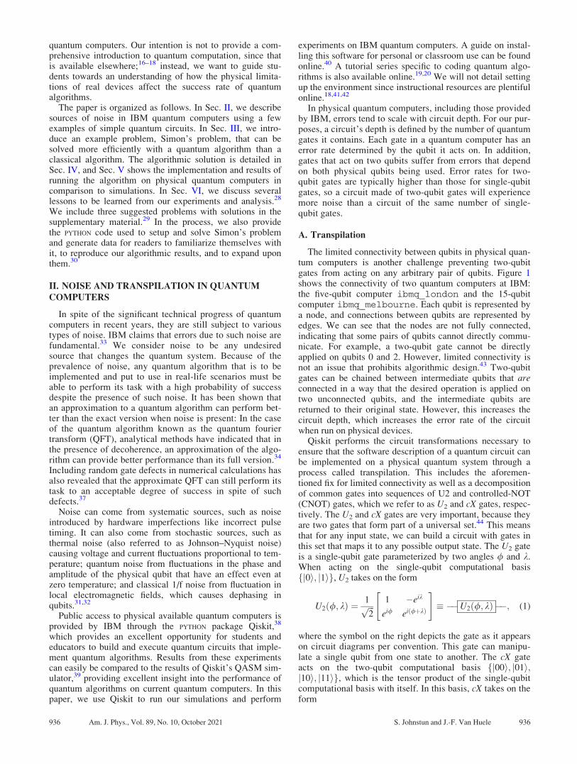
The limited connectivity between qubits in physical quan-tum computers is another challenge preventing two-qubitgates from acting on any arbitrary pair of qubits. Figure 1shows the connectivity of two quantum computers at IBM:the five-qubit computer ibmq_london and the 15-qubitcomputer ibmq_melbourne. Each qubit is represented bya node, and connections between qubits are represented byedges. We can see that the nodes are not fully connected,indicating that some pairs of qubits cannot directly commu-nicate. For example, a two-qubit gate cannot be directlyapplied on qubits 0 and 2. However, limited connectivity isnot an issue that prohibits algorithmic design.43 Two-qubitgates can be chained between intermediate qubits that areconnected in a way that the desired operation is applied ontwo unconnected qubits, and the intermediate qubits arereturned to their original state. However, this increases thecircuit depth, which increases the error rate of the circuitwhen run on physical devices.

Qiskit performs the circuit transformations necessary toensure that the software description of a quantum circuit canbe implemented on a physical quantum system through aprocess called transpilation. This includes the aforemen-tioned fix for limited connectivity as well as a decompositionof common gates into sequences of U2 and controlled-NOT(CNOT) gates, which we refer to as U2 and cX gates, respec-tively. The U2 and cX gates are very important, because theyare two gates that form part of a universal set.44 This meansthat for any input state, we can build a circuit with gates inthis set that maps it to any possible output state. The U2 gateis a single-qubit gate parameterized by two angles / and k.When acting on the single-qubit computational basisfj0i; j1ig, U2 takes on the form

U2ð/; kÞ ¼1ffiffiffi2p 1 �eik

ei/ eið/þkÞ

" #� ��U2ð/; kÞ ��; (1)

where the symbol on the right depicts the gate as it appearson circuit diagrams per convention. This gate can manipu-late a single qubit from one state to another. The cX gateacts on the two-qubit computational basis fj00i; j01i;j10i; j11ig, which is the tensor product of the single-qubitcomputational basis with itself. In this basis, cX takes on theform

936 Am. J. Phys., Vol. 89, No. 10, October 2021 S. Johnstun and J.-F. Van Huele 936

(2)

Note that we have used Qiskit’s little endian convention,which associates the leftmost (more significant) digits in theket with lower qubits on the circuit diagram (higher qubitindex). The qubit with a black dot on the circuit diagram iscalled the control qubit, and the qubit with a circled cross isthe target qubit. The action of a cX gate is to apply a NOT(X) gate to the target qubit in the subspace where the controlqubit is in the j1i state. For example, using the circuit inEq. (2), cXj10i ¼ j10i and cXj01i ¼ j11i, since the left digitin the ket is the target qubit and the right digit is the controlqubit

X¼ 01

10

� ����X��: (3)

In practice, we will see that the increase in circuit depthresulting from transpilation quickly makes the execution ofquantum circuits highly error-prone, rendering their resultsunreliable.

B. Noise demonstration

In this section, we present a few examples to characterizeerrors in IBM quantum computers, both from physical noiseand from algorithmic compromises performed by Qiskit’stranspiler. As we progress through our examples, we willgradually increase the complexity of the circuit, both in num-ber of qubits and number of gates, and see how noiseincreases simultaneously. For explanations and tutorialsabout setting up and running the circuits in our examples,see Chapter 2 of the Qiskit Textbook.18

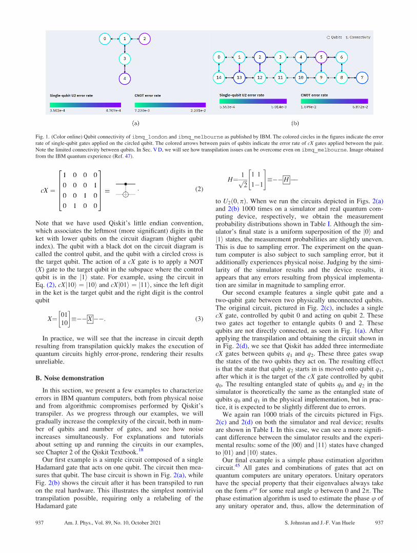
Our first example is a simple circuit composed of a singleHadamard gate that acts on one qubit. The circuit then mea-sures that qubit. The base circuit is shown in Fig. 2(a), whileFig. 2(b) shows the circuit after it has been transpiled to runon the real hardware. This illustrates the simplest nontrivialtranspilation possible, requiring only a relabeling of theHadamard gate

H¼ 1ffiffiffi2p

1 1

1�1

" #���H��

to U2ð0; pÞ. When we run the circuits depicted in Figs. 2(a)and 2(b) 1000 times on a simulator and real quantum com-puting device, respectively, we obtain the measurementprobability distributions shown in Table I. Although the sim-ulator’s final state is a uniform superposition of the j0i andj1i states, the measurement probabilities are slightly uneven.This is due to sampling error. The experiment on the quan-tum computer is also subject to such sampling error, but itadditionally experiences physical noise. Judging by the simi-larity of the simulator results and the device results, itappears that any errors resulting from physical implementa-tion are similar in magnitude to sampling error.

Our second example features a single qubit gate and atwo-qubit gate between two physically unconnected qubits.The original circuit, pictured in Fig. 2(c), includes a singlecX gate, controlled by qubit 0 and acting on qubit 2. Thesetwo gates act together to entangle qubits 0 and 2. Thesequbits are not directly connected, as seen in Fig. 1(a). Afterapplying the transpilation and obtaining the circuit shown inin Fig. 2(d), we see that Qiskit has added three intermediatecX gates between qubits q1 and q2. These three gates swapthe states of the two qubits they act on. The resulting effectis that the state that qubit q2 starts in is moved onto qubit q1,after which it is the target of the cX gate controlled by qubitq0. The resulting entangled state of qubits q0 and q2 in thesimulator is theoretically the same as the entangled state ofqubits q0 and q1 in the physical implementation, but in prac-tice, it is expected to be slightly different due to errors.

We again ran 1000 trials of the circuits pictured in Figs.2(c) and 2(d) on both the simulator and real device; resultsare shown in Table I. In this case, we can see a more signifi-cant difference between the simulator results and the experi-mental results: some of the j00i and j11i states have changedto j01i and j10i states.

Our final example is a simple phase estimation algorithmcircuit.45 All gates and combinations of gates that act onquantum computers are unitary operators. Unitary operatorshave the special property that their eigenvalues always takeon the form eiu for some real angle u between 0 and 2p. Thephase estimation algorithm is used to estimate the phase u ofany unitary operator and, thus, allow the determination of

Fig. 1. (Color online) Qubit connectivity of ibmq_london and ibmq_melbourne as published by IBM. The colored circles in the figures indicate the error

rate of single-qubit gates applied on the circled qubit. The colored arrows between pairs of qubits indicate the error rate of cX gates applied between the pair.

Note the limited connectivity between qubits. In Sec. V D, we will see how transpilation issues can be overcome even on ibmq_melbourne. Image obtained

from the IBM quantum experience (Ref. 47).

937 Am. J. Phys., Vol. 89, No. 10, October 2021 S. Johnstun and J.-F. Van Huele 937

the eigenvalue. This algorithm is incorporated within theaforementioned Shor’s algorithm, as well as in algorithmsused for simulation of quantum systems46 (not to be con-fused with quantum simulators). With larger versions of thisalgorithm, the eigenvalue can be estimated to better accu-racy. An in-depth tutorial on this algorithm can be found inSec. 3.8 of the Qiskit Textbook.18

By comparing Fig. 2(e) and 2(f), we can see that the tran-spiler has significantly increased the depth of the circuit byinserting a large number of cX gates. A comparisonbetween the simulation and experimental results after 1000trials, shown in Table I, indicates that a large amount of

noise has entered the circuit. Whereas in previous exam-ples, we would have been able to guess the correct proba-bility distributions from the data, in this case, the originallyhighly probable j11i state of the first two qubits in the cir-cuit has fallen to a less than 10% probability of beingobserved.

III. SIMON’S PROBLEM

Simon’s problem is a toy computational problem intro-duced in 1994 by Daniel Simon. Its solution is known asSimon’s algorithm. We present it as an example of a problem

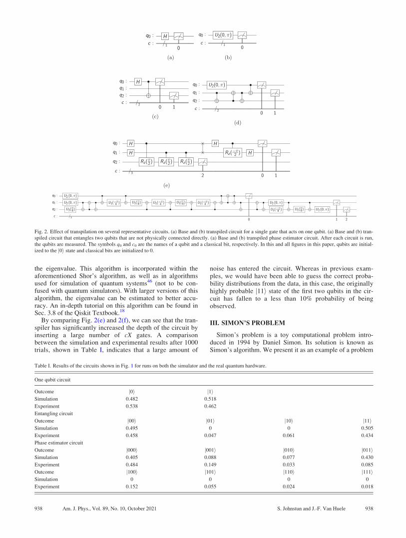
Fig. 2. Effect of transpilation on several representative circuits. (a) Base and (b) transpiled circuit for a single gate that acts on one qubit. (a) Base and (b) tran-

spiled circuit that entangles two qubits that are not physically connected directly. (a) Base and (b) transpiled phase estimator circuit. After each circuit is run,

the qubits are measured. The symbols q0 and c0 are the names of a qubit and a classical bit, respectively. In this and all figures in this paper, qubits are initial-

ized to the j0i state and classical bits are initialized to 0.

Table I. Results of the circuits shown in Fig. 1 for runs on both the simulator and the real quantum hardware.

One qubit circuit

Outcome j0i j1iSimulation 0.482 0.518

Experiment 0.538 0.462

Entangling circuit

Outcome j00i j01i j10i j11iSimulation 0.495 0 0 0.505

Experiment 0.458 0.047 0.061 0.434

Phase estimator circuit

Outcome j000i j001i j010i j011iSimulation 0.405 0.088 0.077 0.430

Experiment 0.484 0.149 0.033 0.085

Outcome j100i j101i j110i j111iSimulation 0 0 0 0

Experiment 0.152 0.055 0.024 0.018

938 Am. J. Phys., Vol. 89, No. 10, October 2021 S. Johnstun and J.-F. Van Huele 938

that is solved more efficiently by a quantum algorithm than aclassical algorithm.

A. Problem description

In Simon’s problem, we are given a function f that maps n-bit integers to ðn�1Þ-bit integers. This function has the prop-erty that there is some nonzero n-bit number a for which, if xand y are any two n-bit numbers, then f ðxÞ ¼ f ðyÞ if and onlyif y ¼ x � a, where � indicates bitwise modulo-2 addition(also known as the XOR operation). In this case, we see thatf ðxÞ ¼ f ðx � aÞ, so the function is periodic under the � oper-ation. The task of Simon’s problem is to find the period a.

B. Classical solution

Classically, if we seek to find the period a, we must testmany different values of x and keep track of x and the outputf(x) until we find a different input y where f ðxÞ ¼ f ðyÞ. Oncethis happens, we find a by calculating x � y. As x is an n-bitnumber, there are 2n possible values to use as input, andeach x has exactly one y for which f ðxÞ ¼ f ðyÞ, so there are2n=2 ¼ 2n�1 pairs of x and y values. This means that wemust compute f(x) for up to 2n�1 distinct values of x in orderto find a, so the algorithm scales exponentially in n, the num-ber of bits in a.

C. Quantum solution

In contrast, the quantum solution to this problem requiresan amount of circuit runs that is only linear in n to find a. Thisis accomplished by putting the n input qubits into a balancedsuperposition of all possible states before calculating f.Putting a register into this state is a standard quantum compu-tational procedure that allows for speedup in many problems.The result of the quantum circuit that implements Simon’salgorithm requires classical postprocessing to find a, since thecircuit does not provide the value of a directly. This meansthat the outcomes measured on the quantum computer need tobe manipulated to extract the value of a. The algorithmicsolution, Simon’s algorithm, is detailed in Sec. IV.

IV. SIMON’S QUANTUM ALGORITHM

A. Quantum operations

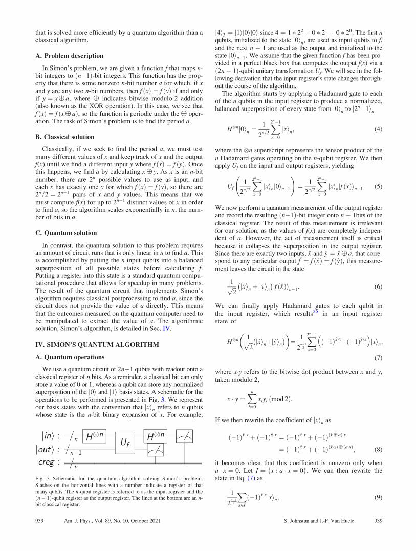
We use a quantum circuit of 2n�1 qubits with readout onto aclassical register of n bits. As a reminder, a classical bit can onlystore a value of 0 or 1, whereas a qubit can store any normalizedsuperposition of the j0i and j1i basis states. A schematic for theoperations to be performed is presented in Fig. 3. We representour basis states with the convention that jxin refers to n qubitswhose state is the n-bit binary expansion of x. For example,

j4i3 ¼ j1ij0ij0i since 4 ¼ 1 � 22 þ 0 � 21 þ 0 � 20. The first nqubits, initialized to the state j0in, are used as input qubits to f,and the next n � 1 are used as the output and initialized to thestate j0in�1. We assume that the given function f has been pro-vided in a perfect black box that computes the output f(x) via að2n� 1Þ-qubit unitary transformation Uf. We will see in the fol-lowing derivation that the input register’s state changes through-out the course of the algorithm.

The algorithm starts by applying a Hadamard gate to eachof the n qubits in the input register to produce a normalized,balanced superposition of every state from j0in to j2n�1in

H�nj0in ¼1

2n=2

X2n�1

x¼0

jxin; (4)

where the �n superscript represents the tensor product of then Hadamard gates operating on the n-qubit register. We thenapply Uf on the input and output registers, yielding

Uf1

2n=2

X2n�1

x¼0

jxinj0in�1

!¼ 1

2n=2

X2n�1

x¼0

jxinjf ðxÞin�1: (5)

We now perform a quantum measurement of the output registerand record the resulting ðn�1Þ-bit integer onto n � 1bits of theclassical register. The result of this measurement is irrelevantfor our solution, as the values of f(x) are completely indepen-dent of a. However, the act of measurement itself is criticalbecause it collapses the superposition in the output register.Since there are exactly two inputs, x and y ¼ x � a, that corre-spond to any particular output f ¼ f ðxÞ ¼ f ðyÞ, this measure-ment leaves the circuit in the state

1ffiffiffi2p jxin þ jyin� �

jf ðxÞin�1: (6)

We can finally apply Hadamard gates to each qubit inthe input register, which results35 in an input registerstate of

H�n 1ffiffiffi2p jxinþjyin� �� �

¼ 1

2nþ1

2

X2n�1

x¼0

ð�1Þx�xþð�1Þy�x

jxin;

(7)

where x�y refers to the bitwise dot product between x and y,taken modulo 2,

x � y ¼Xn

i¼0

xiyi ðmod 2Þ:

If we then rewrite the coefficient of jxin as

ð�1Þx�x þ ð�1Þy�x ¼ ð�1Þx�x þ ð�1Þðx � aÞ�x

¼ ð�1Þx�x þ ð�1Þðx�xÞ� ða�xÞ; (8)

it becomes clear that this coefficient is nonzero only whena � x ¼ 0. Let I ¼ fx : a � x ¼ 0g. We can then rewrite thestate in Eq. (7) as

1

2n�1

2

Xx2I

ð�1Þx�xjxin; (9)

Fig. 3. Schematic for the quantum algorithm solving Simon’s problem.

Slashes on the horizontal lines with a number indicate a register of that

many qubits. The n-qubit register is referred to as the input register and the

ðn� 1Þ-qubit register as the output register. The lines at the bottom are an n-

bit classical register.

939 Am. J. Phys., Vol. 89, No. 10, October 2021 S. Johnstun and J.-F. Van Huele 939

where the summation is taken only over those x values forwhich a�x¼0. If we finally measure the input register andrecord the result onto the n-bit classical register, we are guar-anteed to read out a number z that satisfies z � a ¼ 0. If the cir-cuit is run m times (m � n) and n unique results are recorded,we can build a system of n modulo-2 equations, which we cansolve to find a. This is the classical postprocessing.

Each of the n individual z values has a probability of1=2n�1 of being measured. After m runs of the circuit, theprobability of being able to determine a is no smaller than36

Pmin ¼ 1� 1

2m�nþ1: (10)

We can, thus, determine a to a high probability with a linearnumber of circuit runs, or shots, in n; this probabilityincreases as the quantity m � n increases. For example, ifm ¼ nþ 4, we have over 96% probability of determining aafter m shots. This reveals the exponential speedup of thequantum algorithm over the classical one.

B. Classical postprocessing

After n unique z values have been obtained, we can turnthe system of n equations

z0 � a ¼ 0 mod 2ð Þ;z1 � a ¼ 0 mod 2ð Þ;

..

.

zn � a ¼ 0 mod 2ð Þ;

(11)

into a matrix equation

Za ¼ 0;

where the ith row of the matrix Z is the binary expansion of zi.Applying Gaussian elimination modulo 2 then reveals a singlenontrivial solution which is a, the binary expansion of a.

V. QUANTUM ALGORITHM IMPLEMENTATION

A. Constructing the circuit

We described the transformations needed to implementSimon’s algorithm in Sec. IV. In Appendix B of the

supplementary material,29 we detail the construction of thequantum circuit that performs these operations. Both thebase circuits and transpiled versions of the circuits for n¼ 3and n¼ 6 are also shown in the supplementary material. Aswith the examples in Sec. II B, the transpiler significantlyincreases the quantity of cX gates. The value n¼ 6 waschosen, because it is sufficiently small to allow Simon’sproblem to be solved on a quantum computer of as low as 11qubits. We also constructed a circuit for n¼ 3, the largest nvalue for which Simon’s algorithm can fit on a five-qubitquantum computer.

B. Results

Using Qiskit, we can run the circuits on both the simulatorand the real quantum computing hardware. We perform mshots, where m ranges from three to ten for the n¼ 3 caseand from 6 to 15 in the n¼ 6 case. The lower bounds threeand six are chosen, because they are the minimum number ofshots after which unique determination of a is possible forthe respective problem sizes. The upper bounds of 10 and 15are chosen somewhat arbitrary and simply represent a pointat which further incrementing the number of shots ceases tobe useful.

As a measure of success, we introduce the ratio P of trials,in which we are able to uniquely determine a in postprocess-ing to the total number of trials for that m value. For eachvalue of m, we perform 1000 trials on the simulator with onea value (for n¼ 3) and 100 trials with each of sixteen differ-ent a values (for n¼ 6). The experimental results wereobtained using the five-qubit computer ibmq_ourense forn¼ 3 and the 15-qubit ibmq_16_melbourne for n¼ 6.47

These machines are publicly available and shared with otherusers, so in our trials we experienced queue times that rangedfrom a few seconds to an hour. Due to this limitation, weperformed only a few trials for each m value; 20 trials of mshots were performed in order to determine the success rateof the algorithm.

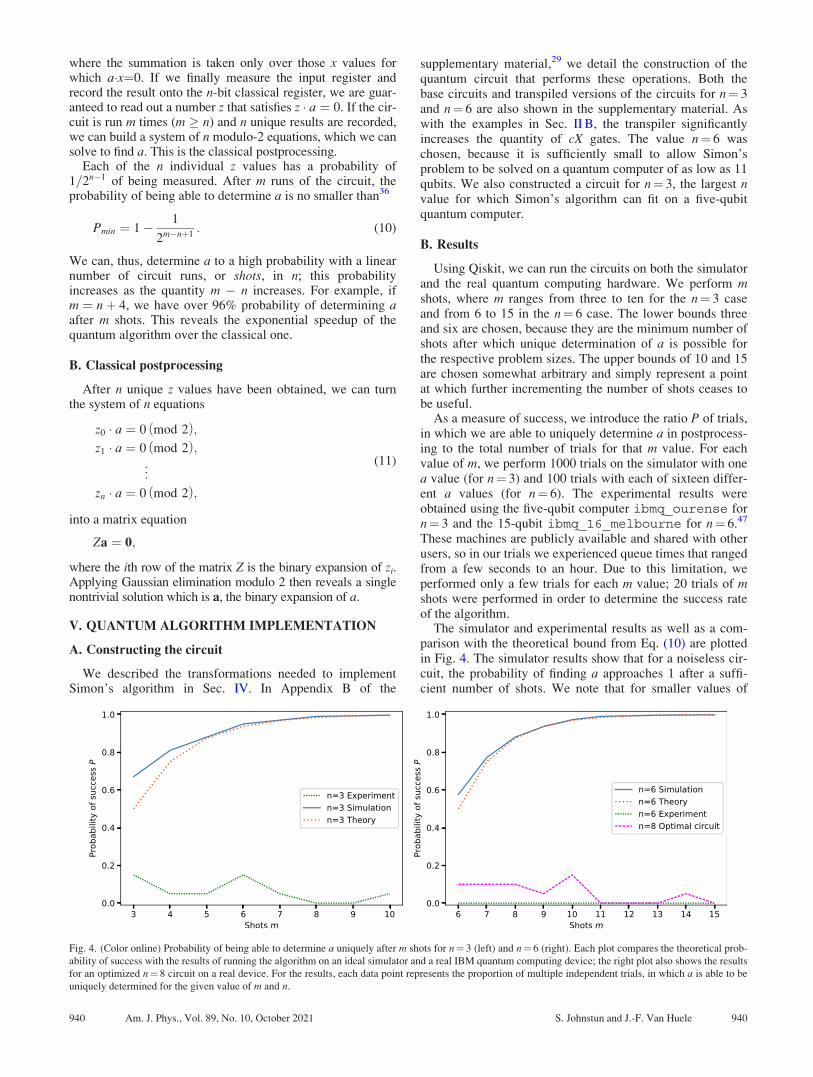
The simulator and experimental results as well as a com-parison with the theoretical bound from Eq. (10) are plottedin Fig. 4. The simulator results show that for a noiseless cir-cuit, the probability of finding a approaches 1 after a suffi-cient number of shots. We note that for smaller values of

Fig. 4. (Color online) Probability of being able to determine a uniquely after m shots for n¼ 3 (left) and n¼ 6 (right). Each plot compares the theoretical prob-

ability of success with the results of running the algorithm on an ideal simulator and a real IBM quantum computing device; the right plot also shows the results

for an optimized n¼ 8 circuit on a real device. For the results, each data point represents the proportion of multiple independent trials, in which a is able to be

uniquely determined for the given value of m and n.

940 Am. J. Phys., Vol. 89, No. 10, October 2021 S. Johnstun and J.-F. Van Huele 940

m � n, the probability of success is slightly better for thesmaller n value. In addition, the simulation probabilities arealways greater than or equal to the theoretical lower bounds,which verifies the correct performance of our implementa-tion in ideal conditions.

The experimental results show a quite low probability ofsuccess with the n¼ 3 algorithm for all values of m; the suc-cess rate never rises above 15%, and it even reaches zero forsome values of m. More significantly, the n¼ 6 algorithmwas never able to complete its task for any value of m. In thenext section, we will address the cause of such lowprobabilities.

C. Error analysis

Due to the nonzero error rate of cX gates on IBM quantumcomputers, we have seen that adding cX gates to the circuitcauses it to perform significantly worse than expected. Forour n¼6 circuit, the transpiler added 57 cX gates to a circuitwhich originally had only 11, for a total of 68 cX gates. Evenif we were to make the most optimistic assumption and takethe minimum error rate of 1:669� 10�2 (as shown in Fig. 1(b))for all cX connections, the probability Pno error;cX that no cXgates error out in the transpiled circuit would be

Pno errors;cX;transpiled ¼ 1� 0:016 69ð Þ62 ¼ 31:8%;

compared to

Pnoerrors;cX;original¼ 1�0:01669ð Þ11¼98:3%;

for the original, nontranspiled circuit. Since the actual errorrate for most of the cX gates in our circuit is actually largerthan this rate, it is practically inevitable that some cX gatewill not perform its task correctly. In terms of our algorithm,this means that the Uf gate, which applies the function f tothe qubits, could be affected so much that it represents anentirely different function.

We have not taken into account the single-qubit U2 errorrate depicted in Fig. 1(b). (Recall that Hadamard gates are con-verted into the equivalent U2ð0; pÞ during transpilation.)Because the circuit requires exactly 2n Hadamard gates and thesingle-qubit nature of these gates avoids any connectivityissues, the U2 gates contribute to less error in the circuit thanthe cX gates. In addition, the greatest U2 error rate of any qubiton ibmq_16_melbourne was 5:014� 10�3 at calibrationtime, which is an order of magnitude lower than the cX errorrates. For our n¼ 6 circuit, then, the worst case estimate of theprobability Pno error;H that no H gate in the circuit has an error is

Pno error;H ¼ 1� 0:005 014ð Þ12 ¼ 94:1%;

which is the same pre- and post-transpilation.The quantity of cX gates added, along with the significant

error rate of the cX gates, is the reason for the difference insuccess between running our algorithm in simulations and ona quantum computer.

D. Overcoming transpilation issues

In an attempt to confirm that the transpiler’s introductionof a significant number of cX gates is responsible for the lowsuccess rates in our algorithm’s performance on a quantumcomputer, we constructed a circuit with a Uf gate

corresponding to the parameter a¼10000001. This particularvalue of a minimizes the number of cX gates necessary, andno ancilla qubits are needed to make up for connectivityrestrictions, so this circuit is expected to perform its task aswell as possible for its n value. This n¼8 circuit is the largestn that can fit on the 15-qubit ibmq_16_melbourne.Using an appropriate mapping, we produced a circuit forn¼8, which is shown in the supplementary material.29 Theonly difference between the pre- and post-transpilation cir-cuits is the change from H gates to U2 gates; the number ofcX gates is the same.

Using the same testing protocol described in the introduc-tory paragraph of Sec. V A, we performed 20 trials of mshots of this n¼ 8 circuit for m ranging from 8 to 17. Theresults of these trials are also plotted in Fig. 4 in comparisonto the n¼ 6 results. The behavior of P as a function of m israther flat and random, which is indicative of small fluctua-tions close to zero. We emphasize the fact that we observeda nonzero probability of success for most values of m, whichis a significant improvement over the results from the n¼ 6case. This result suggests that the increased quantity of cXgates was indeed a major factor in the low success rate wesaw for the n¼ 6 circuit.

The rate of success for this circuit was still rather lowcompared to both simulations on smaller problems and theo-retical estimates. We suspect that this is simply due to theerror rates of gates implemented on ibmq_16_melbourneas discussed in Sec. V C.

VI. DISCUSSION

Our simulations of an ideal quantum computer free ofnoise displayed the correctness of our implementation ofSimon’s algorithm. In the presence of noise on IBM quantumcomputers, we see that the algorithm performs very poorly.In addition to this, the benefit of performing many shotsdiminishes, which means that the algorithm loses its expo-nential speedup over the classical algorithm; ordinarily, thespeedup would originate in the fact that we could guaranteesuccess up to a probability arbitrary close to 1 with a numberof shots linear in n.

Qiskit’s transpiler changes our circuit in a way that allowsfor the physical limitations of the quantum computer to beovercome while theoretically leaving the algorithm unaf-fected, but it also introduces an unruly amount of cX gatesinto the circuit, which are subject to higher error rates thansingle-qubit gates. Since the number of cX gates in Uf scalesat least linearly with n (being the length of the target numbera), the algorithm, therefore, suffers worse performance as nincreases. When we minimized the impact of the transpilerwith a new circuit in Sec. V D, we saw an improved successrate, which supports this conclusion.

We have not discussed error correction protocols in thispaper. Such protocols essentially repeat the algorithm multi-ple times on multiple sets of data, thus increasing the numberof qubits and gates required. However, they may be able tofurther improve the success of the algorithm when it runs onactual quantum computers. In fact, quantum algorithms to beput to commercial use will likely require such protocols intheir implementation. Currently, this requirement of addi-tional qubits means that they are not yet appropriate foraddressing the noise found in the quantum computer weused, but they are promising future prospects for helpingquantum algorithms perform their tasks more reliably. For

941 Am. J. Phys., Vol. 89, No. 10, October 2021 S. Johnstun and J.-F. Van Huele 941

more information on error correction, see the introductoryguide in Ref. 48 and relevant chapters in textbooks on quan-tum computation.16,17

In conclusion, we have introduced the reader to challengesdue to noise and transpilation. These are challenges thathave an important impact on current quantum computers andmust be dealt with in order to understand results. We pre-sented an example problem that was solved efficiently with aquantum algorithm, implemented its algorithmic solution ona simulator and a quantum computer, compared the resultsfrom simulators and experiments, and demonstrated a way tominimize the effects of transpilation.

ACKNOWLEDGMENTS

The authors acknowledge support from the College ofPhysical and Mathematical Sciences at Brigham YoungUniversity. The authors thank Jason Saunders and othermembers of the Quantum Information and Dynamicsresearch group at Brigham Young University for usefuldiscussion and helpful feedback, as well as anonymousreferees for feedback on the manuscript.

a)Electronic mail: scottjohnstun@byu.netb)Electronic mail: vanhuele@byu.edu1Richard P. Feynman, “Quantum mechanical computers,” Opt. News 11,

11–20 (1985).2Peter W. Shor, “Polynomial-time algorithms for prime factorization and

discrete logarithms on a quantum computer,” SIAM Rev. 41, 303–332

(1999).3Edward Gerjuoy, “Shor’s factoring algorithm and modern cryptography.

An illustration of the capabilities inherent in quantum computers,” Am. J.

Phys. 73, 521–540 (2005).4Lov K. Grover, “A fast quantum mechanical algorithm for database

search,” in STOC 1996: Proceedings of the Twenty-Eighth Annual ACMSymposium on Theory of Computing (1996).

5Lov K. Grover, “From Schr€odinger’s equation to the quantum search algo-

rithm,” Am. J. Phys. 69, 769–777 (2001).6Aram W. Harrow, Avinatan Hassidim, and Seth Lloyd, “Quantum algorithm

for linear systems of equations,” Phys. Rev. Lett. 103, 150502 (2009).7Maria Schuld, Ilya Sinayskiy, and Francesco Petruccione, “An introduc-

tion to quantum machine learning,” Contemp. Phys. 56, 172–185 (2014).8Wikipedia has an extensive list of companies involved in quantum

computing or communication <https://en.wikipedia.org/wiki/List_of_

companies_involved_in_quantum_computing_or_communication> (last

accessed December 30, 2020).9Michel H. Devoret, John M. Martinis, and John Clarke, “Measurements of

macroscopic quantum tunneling out of the zero-voltage state of a current-

biased Josephson junction,” Phys. Rev. Lett. 55, 1908–1911 (1985).10Frank Arute et al., “Quantum supremacy using a programmable supercon-

ducting processor,” Nature 574, 505–510 (2019).11Christopher Monroe, Michael G. Raymer, and Jacob Taylor, “The U.S.

National Quantum Initiative: From act to action,” Science 364, 440–442

(2019).12National Academies of Sciences, Engineering, and Medicine, in Quantum

Computing: Progress and Prospects, edited by Emily Grumbling and

Mark Horowitz (The National Academies Press, Washington, DC, 2019).13Frederick W. Strauch, “Resource letter QI-1: Quantum information,” Am.

J. Phys. 84, 495–507 (2016).14D. Candela, “Undergraduate computational physics projects on quantum

computing,” Am. J. Phys. 83, 688–702 (2015).15Yohan Vianna, Mariana R. Barros, and Malena Hor-Meyll, “Classical realiza-

tion of the quantum Deutsch algorithm,” Am. J. Phys. 86, 914–923 (2018).16Isaac Chuang and Michael Nielsen, Quantum Computation and Quantum

Information (Cambridge U. P., Cambridge, 2000).17N. David Mermin, Quantum Computer Science (Cambridge U. P.,

Cambridge, 2007).18Abraham Asfaw et al., Learn quantum computation using Qiskit <https://

qiskit.org/textbook/preface.html> (2020).

19Daniel Koch, Laura Wessing, and Paul M. Alsing, “Introduction to coding

quantum algorithms: A tutorial series using Qiskit,” e-print

arXiv:1903.04359v1 (2019).20Daniel Koch et al., “Fundamentals in quantum algorithms: A tutorial

series using Qiskit continued,” e-print arXiv:2008.10647 (2020).21Javier Rodr�ıguez-Laguna and Silvia N. Santalla, “Building an adiabatic

quantum computer simulation in the classroom,” Am. J. Phys. 86,

360–367 (2018).22N. David Mermin, “From Cbits to Qbits: Teaching computer scientists

quantum mechanics,” Am. J. Phys. 71, 23–30 (2003).23Chih-Chieh Chen et al., “Hybrid classical-quantum linear solver using

Noisy Intermediate-Scale Quantum machines,” Sci. Rep. 9, 16251 (2019).24Sima E. Borujeni et al., “Quantum circuit representation of Bayesian

networks,” Expert Syst. Appl. 176, 114768 (2020).25James R. Wootton, “Benchmarking near-term devices with quantum error

correction,” Quantum Sci. Technol. 5, 044044 (2020).26Announcement by the National Science Foundation on May 18, 2020

<https://www.nsf.gov/news/special_reports/announcements/051820.jsp>(last accessed December 30, 2020).

27Daniel R. Simon, “On the power of quantum computation,” in 1994Proceedings of the 35th Annual Symposium on Foundations of ComputerScience (Institute of Electrical and Electronic Engineers Computer Society

Press, 1994), pp. 115–123.28Some preliminary results of this analysis were submitted for presentation

at the 2020 Annual Conference of the Utah Academy of Sciences, Arts,

and Letters and are included in its proceedings.29See supplementary material at https://www.scitation.org/doi/suppl/

10.1119/10.0006204 for several appendixes that expand and clarify our

discussion and results.30Supplementary material: Demonstration of transpilation effects in

Qiskit <https://github.com/Dot145/QiskitTranspilationNoise/blob/master/

QuantumNoiseInQiskit.ipynb>.”31Philip Krantz et al., “A quantum engineer’s guide to superconducting

qubits,” Appl. Phys. Rev. 6, 021318 (2019).32For an enlightening description of noise sources by Will Oliver, see <https://

youtu.be/aGAb-GbrvMU?t<983> (last accessed December 30, 2020).33See the IBM Research Blog post on dealing with errors in quantum com-

puters a <https://www.ibm.com/blogs/research/2014/06/dealing-with-errors-

in-quantum-computing/> (last accessed December 30, 2020).34Adriano Barenco et al., “Approximate quantum Fourier transform and

decoherence,” Phys. Rev. A 54, 139–146 (1996).35See Eq. (2.37) in Ref. 17.36See Eq. (2.40) and the discussion leading up to it in Ref. 17.37Y. S. Nam and R. Bl€umel, “Robustness of the quantum Fourier transform

with respect to static gate defects,” Phys. Rev. A 89, 042337 (2014).38Gadi Aleksandrowicz et al., “Qiskit: An open-source framework for quan-

tum computing,” Zenodo (2019).39Information on IBM quantum simulators can be found at <https://

www.ibm.com/quantum-computing/simulator/> (last accessed December

30, 2020).40See the Qiskit page with information installing the package at <https://

qiskit.org/documentation/install.html#installing-qiskit> (last accessed

December 30, 2020).41The Qiskit blog on medium is a helpful source for using Qiskit. It can be

found at <https://medium.com/@qiskit> (last accessed December 30, 2020).42Qiskit also has a YouTube channel with video lectures and helpful tutorials

at <https://www.youtube.com/c/qiskit> (last accessed December 30, 2020).43Clara R. Woods, “Evaluating IBM’s quantum compiler and quantum com-

puter architectures as they pertain to quantum walk simulation algo-

rithms,” Honors thesis (University of California, San Diego, 2019).44See the Qiskit webpage on its transpiler, which can be found at <https://qiski-

t.org/documentation/apidoc/transpiler.html#supplementary-information> (last

accessed December 30, 2020).45Krysta M. Svore, Matthew B. Hastings, and Michael Freedman, “Faster

phase estimation,” arXiv:1304.0741 (2013).46Pedro M. Q. Cruz et al., “Optimizing quantum phase estimation for the

simulation of Hamiltonian eigenstates,” Quantum Sci. Technol. 5, 044005

(2020).47These and other quantum computers at IBM can be accessed easily via the

IBM Quantum Experience, located at <https://quantum-computing.ibm.com/>(last accessed December 30, 2020).

48Joschka Roffe, “Quantum error correction: An introductory guide,”

Contemp. Phys. 60, 225–245 (2019).

942 Am. J. Phys., Vol. 89, No. 10, October 2021 S. Johnstun and J.-F. Van Huele 942