Understand Short Texts by Harvesting and Analyzing ... · Compared with documents, short texts are generated in a much larger volume. For example, Google, as the most widely used

1041-4347 (c) 2016 IEEE. Personal use is permitted, but republication/redistribution requires IEEE permission. See http://www.ieee.org/publications_standards/publications/rights/index.html for more information.

This article has been accepted for publication in a future issue of this journal, but has not been fully edited. Content may change prior to final publication. Citation information: DOI 10.1109/TKDE.2016.2571687, IEEETransactions on Knowledge and Data Engineering

1

Understand Short Texts by Harvesting andAnalyzing Semantic Knowledge

Wen Hua, Zhongyuan Wang, Haixun Wang, Member, IEEE, Kai Zheng�, Member, IEEE,and Xiaofang Zhou, Senior Member, IEEE

Abstract—Understanding short texts is crucial to many applications, but challenges abound. First, short texts do not always observe thesyntax of a written language. As a result, traditional natural language processing tools, ranging from part-of-speech tagging to dependencyparsing, cannot be easily applied. Second, short texts usually do not contain sufficient statistical signals to support many state-of-the-artapproaches for text mining such as topic modeling. Third, short texts are more ambiguous and noisy, and are generated in an enormousvolume, which further increases the difficulty to handle them. We argue that semantic knowledge is required in order to better understandshort texts. In this work, we build a prototype system for short text understanding which exploits semantic knowledge provided by a well-knownknowledgebase and automatically harvested from a web corpus. Our knowledge-intensive approaches disrupt traditional methods for taskssuch as text segmentation, part-of-speech tagging, and concept labeling, in the sense that we focus on semantics in all these tasks. Weconduct a comprehensive performance evaluation on real-life data. The results show that semantic knowledge is indispensable for short textunderstanding, and our knowledge-intensive approaches are both effective and efficient in discovering semantics of short texts.

Index Terms—Short text understanding, text segmentation, type detection, concept labeling, semantic knowledge.

F

1 Introduction

I nformation explosion highlights the need for machines to betterunderstand natural language texts. In this paper, we focus

on short texts which refer to texts with limited context. Manyapplications, such as web search and microblogging services etc.,need to handle a large amount of short texts. Obviously, a betterunderstanding of short texts will bring tremendous value.

One of the most important tasks of text understanding is todiscover hidden semantics from texts. Many efforts have beendevoted to this field. For instance, named entity recognition (NER)[1] [2] locates named entities in a text and classifies them intopredefined categories such as persons, organizations, locations,etc. Topic models [3] [4] attempt to recognize “latent topics”,which are represented as probabilistic distributions on words, froma text. Entity linking [5] [6] [7] [8] [9] [10] [11] focuses onretrieving “explict topics” expressed as probabilistic distributionson an entire knowledgebase. However, categories, “latent topics”,as well as “explicit topics” still have a semantic gap with humans’mental world. As stated in Psychologist Gregory Murphy’s highlyacclaimed book [12], “concepts are the glue that holds our mentalworld together”. Therefore, we define short text understanding asto detect concepts mentioned in a short text.

Fig. 1 demonstrates a typical strategy for short text understand-ing which consists of three steps:

• W. Hua is with the School of Information Technology and ElectricalEngineering, University of Queensland, Brisbane, QLD 4072, Australia.E-mail: [email protected].

• Z. Wang is with Microsoft Research Asia, Beijing 100080, China. E-mail:[email protected].

• H. Wang is with Google Research, Mountain View, CA 94043, U.S.A. E-mail: [email protected].

• K. Zheng and X. Zhou are with the School of Information Technologyand Electrical Engineering, University of Queensland, Brisbane, QLD4072, Australia, and are also with the School of Computer Science andTechnology, Soochow University, Suzhou 215021, China. E-mail: {kevinz,zxf}@itee.uq.edu.au.

• Text Segmentation - divide a short text into a collection ofterms (i.e., words and phrases) contained in a vocabulary(e.g., “book disneyland hotel california” is segmented as{book disneyland hotel california});

• Type Detection - determine the types of terms and rec-ognize instances (e.g., both “disneyland” and “california”are recognized as instances in Fig. 1, while “book” isrecognized as a verb and “hotel” a concept);

• Concept Labeling - infer the concept of each instance (e.g.,“disneyland” and “california” refer to the concept themepark and state respectively in Fig. 1).

Overall, three concepts are detected from short text “book dis-neyland hotel california” using this strategy, namely theme park,hotel, and state in Fig. 1.

book[v] disneyland[e](park) hotel[c] california[e](state)

book[v] disneyland[e] hotel[c] california[e]

book disneyland hotel california

book disneyland hotel california

Fig. 1. An example of short text understanding.

Although the three steps for short text understanding soundquite simple, challenges still abound and new approaches mustbe introduced to handle them. In the following, we use severalexamples to illustrate such a need.Challenge 1 (Ambiguous Segmentation).

• “april in paris lyrics” vs. “vacation april in paris”

Both a term and its sub-terms can be contained in the vo-cabulary, leading to multiple possible segmentations for a shorttext. However, a valid segmentation should maintain semanticcoherence. For example, two segmentations can be derived from“april in paris lyrics”, namely {april in paris lyrics} and {april parislyrics}. However, the former is a better segmentation accordingto the knowledge that “lyrics” is more semantically related with



2

songs (“april in paris”) than months (“april”) or cities (“paris”).Traditional Longest Cover method, which is widely-adopted fortext segmentation [13] [14] [15] [16] [17], seeks for longestterms contained in a vocabulary. It ignores the requirement ofsemantic coherence, and thus will lead to incorrect segmentationssometimes. In the case of “vacation april in paris”, the LongestCover method segments it as {vacation april in paris} which isobviously an incoherent segmentation.

Challenge 2 (Noisy Short Text).

• “new york city” vs. “nyc” vs. “big apple”

In order to find the best segmentation for a given text by con-sidering semantic coherence, we first need to extract all candidateterms. It can be easily and efficiently done by building a hash indexon the entire vocabulary. However, short texts are usually informaland error-prone, full of abbreviations, nicknames, misspellings,etc. For example, “new york city” is usually abbreviated to “nyc”and known as “big apple”. This calls for the vocabulary to incor-porate as much information about abbreviations and nicknames aspossible. Meanwhile, approximate term extraction is also requiredto handle misspellings in short texts.

Challenge 3 (Ambiguous Type).

• “pink[e](singer) songs” vs. “pink[ad j] shoes”

We tag terms with lexical types (i.e., POS tags) and semantictypes (i.e., attribute, concept, and instance). We will explain whywe consider these types and how they contribute to short textunderstanding in Sec. 3.1.2. A term can belong to several types,and its best type in a short text depends on context semantics. Forexample, “pink” in “pink songs” refers to a famous singer andthus should be labeled as an instance, whereas it is an adjectivein “pink shoes” describing the color of shoes. Traditional POStaggers determine lexical types based on linguistic rules [18] [19][20] [21] [22] or lexical and sequential probabilities learned froma labeled corpora [23] [24] [25] [26] [27] [28] [29]. However, suchsurface features are inapplicable in short texts, due to the fact thatshort texts do not always observe the syntax of a written language.Consider “pink songs” as an example. Since both the probability of“pink” as an adjective and the probability of an adjective precedinga noun are relatively high, traditional POS taggers will mistakenlylabel “pink” in “pink songs” as an adjective. Another limitationof POS tagging is that it cannot distinguish semantic types which,however, is very important for short text understanding, as will bediscussed in Sec. 3.1.2.

Challenge 4 (Ambiguous Instance).

• “read harry potter[e](book)” vs. “watch harry potter[e](movie)”vs. “age harry potter[e](character)”

An instance (e.g., “harry potter”) can belong to multipleconcepts (e.g., book, movie, character, etc.). We can retrieve suchone-to-many mappings between instances and concepts directlyfrom existing knowledgebases. However, instances might refer todifferent concepts when context varies. Some methods [15] [16][17] attempt to eliminate instance ambiguity based on similar orrelated instances, but the number of instances that can be retrievedfrom a short text is usually limited, making these methods in-applicable to instance disambiguation in short texts. We observethat other terms, such as verbs, adjectives, and attributes, can alsohelp with instance disambiguation. For example, “harry potter” is

a book in “read harry potter”, a movie in “watch harry potter”,and a character in “age harry potter”. Humans can successfullyrecognize the most appropriate concept for an instance within aspecific short text, since we have the knowledge about semantic re-latedness between various types of terms. However, it is nontrivialfor machines to disambiguate instances without such knowledge.Challenge 5 (Enormous Volume).

Compared with documents, short texts are generated in a muchlarger volume. For example, Google, as the most widely used websearch engine as of 2014, received over 3 billion search queriesdaily1. Twitter also reported in 2012 that it attracted more than 100million users who posted 340 million tweets per day2. Therefore,a feasible framework for short text understanding should be ableto handle short texts in real time. However, a short text can havetens of possible segmentations, a term can be labeled with multipletypes, and an instance can refer to millions of concepts. Hence, itis extremely time-consuming to eliminate these ambiguities andachieve the best semantic interpretation for a short text.

Contributions. In this work, we argue that semantic knowledge isindispensable for short text understanding, which in turn benefitsmany real-world applications that need to handle a large amountof short texts. According to the above discussion, three typesof knowledge are required to cope with the challenges in shorttext understanding: 1) a comprehensive vocabulary; 2) mappingsbetween instances and concepts; 3) semantic coherence betweenterms. We will describe how we harvest these knowledge inSec. 3.1.1, Sec. 3.1.3, and Sec. 4.1.1 respectively. Based on theacquired knowledge, we propose knowledge-intensive approachesto understand short texts both effectively and efficiently, whichwill be described in Sec. 4.2. Overall, our contributions in thiswork are threefold:

• We observe the prevalence of ambiguity in short texts andthe limitations of traditional approaches in handling them;

• We achieve better accuracy of short text understanding byharvesting semantic knowledge from web corpus and exist-ing knowledgebases, and introducing knowledge-intensiveapproaches based on lexical-semantic analysis;

• We improve the efficiency of our approaches to facilitateonline instant short text understanding.

The rest of this paper is organized as follows: in Sec. 2, webriefly summarize related work in the literature of text processing;then we introduce some notations used in this paper, and definethe problem of short text understanding formally in Sec. 3; ourapproaches and experiments are described in Sec. 4 and Sec.5 respectively, followed by a brief conclusion and discussion offuture work in Sec. 6.

2 RelatedWorkIn this section, we discuss related work in three aspects: textsegmentation, POS tagging, and semantic labeling.

Text Segmentation. We consider text segmentation as to dividea text into a sequence of terms. Existing approaches can be clas-sified into two categories: statistical approaches and vocabulary-based approaches. Statistical approaches, such as N-gram Model[30] [31] [32], calculate the frequencies of words co-occurringas neighbors in a training corpus. When the frequency exceeds a

1. https://en.wikipedia.org/wiki/Google Search2. https://en.wikipedia.org/wiki/Twitter



3

predefined threshold, the corresponding neighboring words can betreated as a term. Vocabulary-based approaches extract terms ina streaming manner by checking for existence or frequency of aterm in a predefined vocabulary. In particular, the Longest Covermethod, which is widely-adopted for text segmentation [13] [14][15] [16] [17] due to its simplicity and real-time nature, searchesfor longest terms contained in a vocabulary while scanning thetext. The most obvious drawback of existing methods for textsegmentation is that they only consider surface features and ignorethe requirement of semantic coherence within a segmentation. Thiswill lead to incorrect segmentations in cases such as “vacationapril in paris” described in Challenge 1. To this end, we proposeto exploit context semantics when conducting text segmentation.

POS Tagging. POS tagging determines lexical types (i.e., POStags) of words in a text. Mainstream POS tagging algorithmsfall into two categories: rule-based approaches and statisticalapproaches. Rule-based POS taggers attempt to assign POS tagsto unknown or ambiguous words based on a large number of hand-crafted [18] [19] or automatically learned [20] [21] [22] linguis-tic rules. Statistical POS taggers avoid the cost of constructingtagging rules by building a statistical model automatically from acorpora and labeling untagged texts based on those learned statisti-cal information. Most of the widely-adopted statistical approachesemploy the well-known Markov Model [23] [24] [25] [26] [27][28] [29] which learns both lexical probabilities (P(tag|word))and sequential probabilities (P(tagi|tagi−1, tagi−2, ..., tagi−n)) froma labeled corpora and tags a new sentence by searching for tagsequence that maximizes the combination of lexical and sequentialprobabilities. Note that both rule-based and statistical approachesto POS tagging rely on the assumption that texts are correctlystructured. In other words, texts should satisfy tagging rulesor sequential relations between consecutive tags. However, thisis not always the case for short texts. More importantly, allof the aforementioned work only considers lexical features andignores word semantics. This will lead to mistakes sometimes, asillustrated in the case of “pink songs” described in Challenge 3.Our work attempts to build a tagger which considers both lexicalfeatures and underlying semantics for type detection.

Semantic Labeling. Semantic labeling discovers hidden se-mantics from a natural language text. According to the repre-sentation of semantics, existing work on semantic labeling canbe roughly classified into three categories, namely named entityrecognition (NER), topic modeling, and entity linking. NER lo-cates named entities in a text and classifies them into predefinedcategories (e.g., persons, organizations, locations, times, quantitiesand percentages, etc.) using linguistic grammar-based techniquesas well as statistical models like CRF [1] and HMM [2]. Topicmodels [3] [4] attempt to recognize “latent topics”, which arerepresented as probabilistic distributions on words, based onobservable statistical relations between texts and words. Entitylinking [5] [6] [7] [8] [9] [10] [11] employs existing knowl-edgebases and focuses on retrieving “explict topics” expressedas probabilistic distributions on the entire knowledgebase. Despitethe high accuracy that has been achieved by existing work onsemantic labeling, there are still some limitations. First, categories,“latent topics”, as well as “explicit topics” are different fromhuman-understandable concepts. Second, short texts do not alwaysobserve the syntax of a written language which, however, is anindispensable feature used in mainstream NER tools. Third, shorttexts usually do not contain sufficient content to support statisticalmodels like topic models.

The work most related to ours are conducted by Song etal. [16] and Kim et al. [17] respectively, which also representsemantics as concepts. [16] employs the Bayesian Inference mech-anism to conceptualize instances and short texts, and eliminatesinstance ambiguity based on homogeneous instances. [17] cap-tures semantic relatedness between instances using a probabilistictopic model (i.e., LDA), and disambiguates instances based onrelated instances. In this work, we observe that other terms, suchas verbs, adjectives, and attributes, can also help with instancedisambiguation. Therefore, we incorporate type detection intoour framework for short text understanding and conduct instancedisambiguation based on various types of context information.

3 Problem StatementIn this section, we briefly introduce some concepts and notationsused in the paper. Then we formally define the problem of shorttext understanding, and give an overview of our framework.

3.1 Preliminary Concepts

TABLE 1Summary of concepts and notations.

Definition Examples short text book hotel californiap segmentation {book hotel california}t term hotel,california,hotel californiat typed-term book[v],book[c],book[e]

t.r type v,adj,att,c,et. ~C concept cluster vector ({theme park,park},{company}...)

3.1.1 Vocabulary, Term, and SegmentationDefinition 1 (vocabulary). A vocabulary is a collection of words

and phrases (of a certain language).

We download a list of English verbs and adjectives from anonline dictionary - YourDictionary3, and harvest a collection ofattributes, concepts, and instances from a well-known knowledge-base - Probase4. Altogether, they constitute our vocabulary. Tocope with the noise contained in short texts, we further extendthe vocabulary to incorporate abbreviations and nicknames ofinstances. These can be obtained from web corpus or existingknowledgebases. In particular, we construct a list of synonyms5

from Wikipedia’s redirect links, disambiguation links, as wellas hypertexts and hyperlinks between Wikipedia articles. Forexample, from the redirect information between “nyc” and “newyork city”, we know that “nyc” is an abbreviation of “new yorkcity”; similarly, form the disambiguation link of “big apple”, weobtain that “big apple” is a nickname of “new york city”.Definition 2 (term). A term t is an entry in the vocabulary.

We represent a term as a sequence of words, and denote |t| asthe length (number of words) of term t. Example terms are “hotel”,“california”, and “hotel california”, etc.Definition 3 (segmentation). A segmentation p of a short text is a

sequence of terms p = {ti|i = 1, ..., l} such that:

3. http://www.yourdictionary.com/

4. http://research.microsoft.com/en-us/projects/probase/

5. The synonym dictionary is publicly available at http://probase.msra.cn/dataset.aspx.



4

1) terms cannot overlap with each other, i.e., ti ∩ ti+1 = ∅,∀i;2) every non-stopword in the short text should be covered bya term, i.e., s −

⋃li=1 ti ⊂ stopwords.

For example, a possible segmentation of “vacation april inparis” is {vacation april paris}, where only stopword “in” is ignoredfrom the original short text. For “new york times square,” althoughboth “new york times” and “times square” are terms in ourvocabulary, {new york times times square} is invalid according toour restrictions because the two terms overlap with each other.

3.1.2 Type and Typed-Term

Definition 4 (type). Type denotes the lexical or semantic role aterm plays in a text.

Lexical types include verb and adjective. We consider lexicaltypes in this work for two reasons. First, verbs and adjectivescan help with instance disambiguation, as discussed in Challenge4. Second, one of the most important applications of short textunderstanding is to calculate semantic similarity between shorttexts, whereas incorrect detection of lexical types will causemistakes in calculating semantic similarity. Consider the followingexample, wherein “watch” is a verb in “watch free movie” while aconcept in “watch omega”. These two short texts are semanticallydissimilar, as the former is about watching a free movie whilethe latter searches for a famous brand of watch called “omega”.However, if we do not consider lexical types and label “watch”in “watch free movie” as an instance or a concept, it will lead toincorrectly high similarity between these two short texts.

• “watch[v] free movie” vs. “watch[c] omega”

Semantic types include attribute, concept, and instance. POStagging only distinguishes lexical types and ignores the differencesbetween semantic types, which will also cause mistakes in calcu-lating semantic similarity between short texts. In the examplesbelow, “population” can be both an attribute of concept countryand an instance of concept geographic statistics. The first pair ofshort texts are both about geographic statistics of a country (i.e.,same concept but different attributes), while the second pair ofshort texts are about statistical information of a country and ananimal respectively (i.e., same attribute but different concepts).This leads to larger semantic similarity in the first pair than thesecond pair. We can see that concepts and instances contributemore to the semantics of a short text than attributes, which verifiesthe necessity to distinguish semantic types.

• “population china” vs. “climate china”• “population china” vs. “population panda”

Definition 5 (typed-term). A typed-term t refers to a term with aspecific type t.r.

A term can be labeled with multiple types and thus can be mappedto multiple typed-terms. We denote the set of possible typed-terms for a term as T = {ti|i = 1, ...,m}, which can be obtaineddirectly from the vocabulary. For example, we observe that term“book” appears in verb-list, concept-list as well as instance-listof our vocabulary, thus the possible typed-terms of “book” are{book[v],book[c],book[e]}.

3.1.3 Knowledgebase and Concept Cluster Vector

Definition 6 (knowledgebase). A knowledgebase stores mappingsbetween instances and concepts. Some existing knowledge-bases also associate each concept with certain attributes.

In this work, we use Probase [33] as our knowledgebase.Probase is a huge semantic network of concepts (e.g., country),instances (e.g., china) and attributes (e.g., population). It mainlyfocuses on two types of relationships, namely the isA relationshipbetween instances and concepts (e.g., china isA country) and theisAttributeOf [34] relationship between attributes and concepts(e.g., population isAttributeOf country). We use Probase for tworeasons. First, Probase’s broad coverage of concepts makes itmore representative of humans’ mental world, in comparison withother knowledgebases such as Freebase, WordNet, DBPedia, etc.Knowledge in Probase is acquired automatically from a corpusof 1.68 billion webpages, and it contains 2.7 million conceptsand 16 million instances, which results in more than 20.7 millionmappings between instances and concepts. Second, unlike tradi-tional knowledgebases that simply treat knowledge as black orwhite, Probase quantifies many measures such as popularity andtypicality which are important to cognition.

• Popularity p(c|e), e.g., p(c = company|e = apple) mea-sures how likely people will think of the concept “com-pany” when they see the term “apple”;

• Typicality p(e|c), e.g., p(e = steve jobs|c = ceo) measureshow likely “steve jobs” will come into mind when peoplethink about the concept “ceo”.

We can directly obtain the semantics (i.e., concepts) of aninstance from Probase. However, some of Probase’s concepts areactually similar. For example, “apple” can belong to conceptscompany, it company, big company, software company, etc. Inorder to find the most appropriate semantics of “apple” in shorttext “price apple”, all these concepts must be checked and removedone by one, which is obviously a waste of time. To representsemantics in a more compact manner and to speed up the pro-cess of instance disambiguation, we employ the K-Medoids [35]algorithm to cluster similar concepts contained in Probase. Ourintuition is that if two concepts share many instances, they aresimilar to each other. Readers can refer to [36] for more details onconcept clustering.

Definition 7 (concept cluster vector). We represent the se-mantics of a typed-term as a concept cluster vector t. ~C =

(〈C1,W1〉, 〈C2,W2〉, ..., 〈CN ,WN〉), where Ci represents a con-cept cluster and Wi its weight, as formally defined in Eq. 1.

t. ~C =

∅ t.r ∈ {v, ad j, att}(< C, 1 > |t ∈ C) t.r = c(< Ci,Wi > |i = 1, ...,N) t.r = e

(1)

In Eq. 1, we distinguish three circumstances: 1) verbs, adjectives,and attributes have no hypernyms in Probase, thus we specificallydefine their concept cluster vectors as empty; 2) for a concept,only the concept cluster it belongs to will be assigned with theweight 1 and all the other concept clusters will be assigned withthe weight 0; 3) for an instance, we retrieve its concepts fromProbase and weigh each concept cluster by the summation ofweights of containing concepts. More formally, Wi =

∑c∈Ci

p(c|t)where p(c|t) is the popularity score harvested by Probase.



5

3.2 Problem Definition and Framework Overview

Definition 8 (Short Text Understanding). Given a short text swritten in a natural language, we generate a semantic interpre-tation of s represented as a sequence of typed-terms namelys = {ti|i = 1, ..., l}, and the semantics of each instance is labeledwith the top-1 concept cluster.

As shown in Fig. 1, the semantic interpretation of short text“book disneyland hotel california” is {book[v] disneyland[e](park)

hotel[c] california[e](state)}. We divide the task of short text un-derstanding into three subtasks corresponding to the three stepsmentioned in Sec. 1 respectively:

• Text Segmentation - given a short text, find the mostsemantically coherent segmentation;

• Type Detection - for each term, detect its best type;• Concept Labeling - for each ambiguous instance, re-rank

its concept clusters according to the context.

Fig. 2. Framework overview.

Fig. 2 illustrates our framework for short text understanding.In the offline part, we construct index on the entire vocabulary andacquire knowledge from web corpus and existing knowledgebases.Then, we pre-calculate semantic coherence between terms whichwill be used for online short text understanding. In the onlinepart, we perform text segmentation, type detection, and conceptlabeling, and generate a semantically coherent interpretation for agiven short text.

4 MethodologyIn this section, we describe the details of our framework forshort text understanding, i.e., the offline and online processingrespectively.

4.1 Offline Processing

A prerequisite to short text understanding is the knowledge aboutsemantic relatedness between terms. We describe how we con-struct the co-occurrence network6 and quantify semantic coher-ence in this section. After that, we introduce the indexing strategyto allow for approximate term extraction on the vocabulary, aswell as the approach to determine instance ambiguity.

6. The co-occurrence network is publicly available at http://probase.msra.cn/dataset.aspx.

4.1.1 Constructing Co-occurrence NetworkWe construct a co-occurrence network to model semantic related-ness. The co-occurrence network can be regarded as an indirectedgraph, where nodes are typed-terms and edge weight w(x, y)formulates the strength of semantic relatedness between typed-terms x and y. We observe that

• Terms of different types occur in different contexts. InFig. 3, “watch” as a verb co-occurs with concept moviewhile “watch” as an instance co-occurs with “buy” and“price”. Therefore, the co-occurrence network should beconstructed between typed-terms instead of terms;

• The more frequently two typed-terms co-occur in a sen-tence, the higher the semantic relatedness will be;

• The closer two typed-terms appear in a sentence, the higherthe semantic relatedness will be;

• Common terms (e.g., “item” and “object”) which co-occurwith almost every other term are meaningless in modelingsemantic relatedness, thus the corresponding edge weightsshould be penalized.

Based on these observations, we build a co-occurrence net-work as follows: 1) We scan every distinct sentence from a webcorpus, and obtain part-of-speech tags using Stanford POS tagger.For words tagged as verbs or adjectives, we derive their stemsand get a collection of verbs and adjectives. For noun phrases, wecheck them in the vocabulary and determine their types (attribute,concept, instance) collectively by minimizing topical diversity.Our intuition is that the number of topics mentioned in a sentenceis usually limited. For example, “population” can be an attributeof country as well as an instance of geographical data. Assumethat the collection of noun phrases parsed from a sentence is{“china”,“population”}, then “population” should be labeled as anattribute in order to limit the topic of the sentence to be countryonly. Using this approach, we can obtain a set of attributes,concepts and instances. Take “Outlook.com is a free personalemail from Microsoft” as another example. The collection oftyped-terms we get after analyzing this sentence is {outlook[e],f ree[ad j], personal[ad j], email[c], microso f t[e]}. 2) Given the setof typed-terms derived from a sentence, we add a co-occur edgebetween each pair of typed-terms. To estimate edge weight, wefirst calculate the frequency of two typed-terms appearing togetherusing the following formula:

fs(x, y) = ns · e−dists(x,y) (2)

Here, ns is the number of times sentence s appears in the webcorpus, and dists(x, y) is the distance between typed-terms x and y(i.e., number of typed-terms in-between) in that sentence. e−dists(x,y)

is used to penalize distant co-occurrence. We then aggregatefrequencies among sentences, and weigh each edge by a modifiedtf-idf formula.

f (x, y) =∑

s

fs(x, y) (3)

w(x, y) =f (x, y)∑z f (x, z)

· logN

Nnei(y)(4)

Here, f (x,y)∑z f (x,z) estimates the probability that humans think of typed-

term y when seeing x. N is the total number of typed-termscontained in the co-occurrence network, and Nnei(y) is the numberof co-occurrence neighbors of y. Therefore, the idf part of thisformula penalizes typed-terms that co-occur with almost everyother typed-term.



6

There are some obvious drawbacks in the above approach.First, the number of typed-terms is extremely large. Recall thatProbase contributes 2.7 million concepts and 16 million instancesto our vocabulary. This will increase storage cost and affect theefficiency of calculation on the network. Second, concept-levelco-occurrence is more useful for short text understanding, whensemantic coherence is considered. Therefore, we compress theoriginal co-occurrence network by retrieving concepts of eachinstance from Probase, and then grouping similar concepts to-gether into concept clusters. The nodes in the compressed versionof the co-occurrence network are verbs, adjectives, attributes andconcept clusters, and the edge weights (i.e., w(x,C) and w(C1,C2))are aggregated from the original network. In Fig. 3, “lyrics” co-occurs with concept song as well as instances “april in paris” and“hotel california” in the original co-occurrence network. Whereasin the compressed version, it only co-occurs with concept clustersong. In this way, we reduce the size of the co-occurrence networkto a large extent. We use the compressed network in the remainingof this work to estimate semantic coherence.

watch[v]

buy[v]

age[att]

lyrics[att]

harry potter[e]

hotel california[e]

april in paris[e]

product[c]

price[att]

ipad[e]

omega[e]

watch[e]

brand[c]

company[c]

apple[e]

google[e]

read[v]

song[c]

watch[v]

read[v]

movie

book

character

age[att]

song

lyrics[att]

price[att]

product

brand

buy[v]

company

Fig. 3. An example of compressed co-occurrence network.

4.1.2 Scoring Semantic CoherenceWe define Affinity Score (AS) to measure semantic coherencebetween typed-terms. In this work, we consider two types ofcoherence: similarity and relatedness (co-occurrence). We believethat two typed-terms are coherent if they are semantically similaror they often co-occur on the web. Therefore, the Affinity Scorebetween typed-terms x and y can be calculated as follows:

S (x, y) = max(S sim(x, y), S co(x, y)) (5)

In Eq. 5, S sim(x, y) is the semantic similarity between typed-termsx and y, which can be calculated directly as the cosine similaritybetween their concept cluster vectors.

S sim(x, y) = cosine(x. ~C, y. ~C) (6)

S co(x, y) measures semantic relatedness between typed-terms xand y. We denote the co-occur concept cluster vector of typed-term x as ~Cco(x) which can be retrieved from the compressed co-occurrence network, and the concept cluster vector of typed-termy as y. ~C. We observe that the larger the overlapping between thesetwo concept cluster vectors, the stronger the relatedness betweentyped-terms x and y. Therefore, we calculate S co(x, y) as follows:

S co(x, y) = cosine( ~Cco(x), y. ~C) (7)

4.1.3 Indexing Vocabulary for Approximate Term ExtractionApproximate term extraction aims to locate substrings in a textwhich are similar to terms contained in a predefined vocabulary.To quantify the similarity between two strings, many similarityfunctions have been proposed including token-based similarity

functions (e.g., jaccard coefficient) and character-based similarityfunctions (e.g., edit distance). Due to the prevalence of mis-spellings in short texts, we use edit distance as our similarityfunction to facilitate approximate term extraction.

There have been some recent studies on approximate termextraction. We adopt and extend the trie-based method [37] inthis work, considering its smaller index size compared with otherapproaches such as NGPP [38] and Faerie [39], as well as itsefficiency for large edit distance threshold. Specifically, given anedit distance threshold τ, we divide each term into τ + 1 segmentsevenly. The pigeonhole principle guarantees that if a substring issimilar to a term with respect to τ, it must contain at least onesegment of that term. We build a segment-based inverted indexon the entire vocabulary, where the entries are segments and eachsegment is associated with an inverted list of terms containingthe segment. Given a short text, we adopt the search-extensionalgorithm proposed in [37] to find all possible terms. In otherwords, we first enumerate every substring of a short text and checkwhether it matches a segment using the trie structure. In this way,we obtain a set of segments contained in the short text. Thenfor each segment and the corresponding substring, we extend thesubstring to a longer substring similar to a term in the inverted list.

The most notable limitation of the existing trie-based frame-work is that it utilizes one specific edit distance threshold τ. How-ever, our vocabulary contains a large amount of abbreviations aswell as multi-word instances which require different edit distancethresholds. For example, in order to recognize misspelled multi-word instances, we sometimes need a large edit distance thresholdof at least 2. But when we apply the same edit distance thresholdto abbreviations, it will lead to mistakes (e.g., “nyc” and “ntu”will be regarded as similar). To this end, we extend the trie-basedframework to allow for various edit distance thresholds at the sametime. The problem is how to determine the value of τ for differentterms. It can be expected that τ depends on the length of terms.In other words, the longer a term is, the more possible it willbe misspelled and the more mistakes there will be. Therefore,we collect a large-scale short text dataset from search enginesand microblogging sites, and invite colleagues to label misspelledterms along with their edit distances. We observe a near step-likedistribution between edit distance and term length, which is thenused as our guideline for determining edit distance threshold fordifferent terms.

4.1.4 Determining Instance AmbiguityThe focus of concept labeling is instance disambiguation, makingit important to determine whether an instance is ambiguous or not.Handling unambiguous instances is a waste of time and will causeover-filtering sometimes. A straightforward approach to determineinstance ambiguity is to check the number of concepts (or conceptclusters) it belongs to. However, the accuracy of such a methodis highly dependent on the granularity of concept space in aknowledgebase. A coarse-grained knowledgebase will miss someambiguous instances, while a fine-grained knowledgebase mightlead to false positive (i.e., an unambiguous instance is incorrectlyrecognized as ambiguous). In this work, we adopt a fine-grainedknowledgebase, Probase, with a huge coverage of 2.7 millionconcepts and 5000 concept clusters. We introduce a method to re-duce false positive in determining instance ambiguity by analyzingvarious correlations between concept clusters. One thing to noteis that instance ambiguity can be influenced by spatial-temporalfeatures. For example, “apple” was not an ambiguous instance



7

before the year 1976 when the Apple Company was founded.As another example, “river bank” is ambiguous only in NorthernCalifornia where it can refer to both the sloped side of a river anda regional bank. Our current work focus on understanding generalshort texts without any spatial-temporal information, but we leaveit as a future work.

region

country state city

creature

animal

predator

crop food

fruit vegetable meat

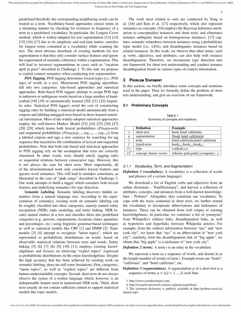
Fig. 4. Examples of senses as hierarchies of concept clusters.

Ambiguity is a subjective concept. We conduct a user studyto learn how humans determine instance ambiguity. We provideannotators with a set of instances together with their top-10concept clusters, and ask them to label whether these instancesare ambiguous or not. According to the user study results, weobtain three useful findings: 1) All annotators regard instancessuch as “dog” as unambiguous although they belong to multipleconcept clusters. These concept clusters (e.g., predator, animal,creature, etc.) actually constitute a hierarchy which we denote asa Sense in this work, as shown in Fig. 4. 2) Some of the annotatorslabel instances such as “google” as unambiguous, although theybelong to multiple senses. These senses (e.g., search engine andcompany) are actually highly related with each other since theyhave a large proportion of common instances. 3) All annotatorslabel instances such as “apple” as ambiguous because they belongto multiple unrelated senses (e.g., fruit and company). Based onthese findings, we introduce three levels of instance ambiguity,and propose methods to determine ambiguity level by analyzingthe hierarchical and overlapping relationships between conceptclusters.

• Ambiguity level 0 refers to instances that most peopleregard as unambiguous. These instances contain only onesense, such as “dog” (animal) and “california” (state);

• Ambiguity level 1 refers to instances that both ambiguousand unambiguous make sense. These instances usuallycontain more than one senses, but all of these sensesare related to some extent, such as “google” (company &search engine) and “nike” (brand & company);

• Ambiguity level 2 refers to instances that most peoplethink as ambiguous. These instances contain two or moreunrelated senses, such as “apple” (fruit & company) and“jaguar” (animal & company).

In this work, we only focus on disambiguation of instances thatbelong to ambiguity level 2.

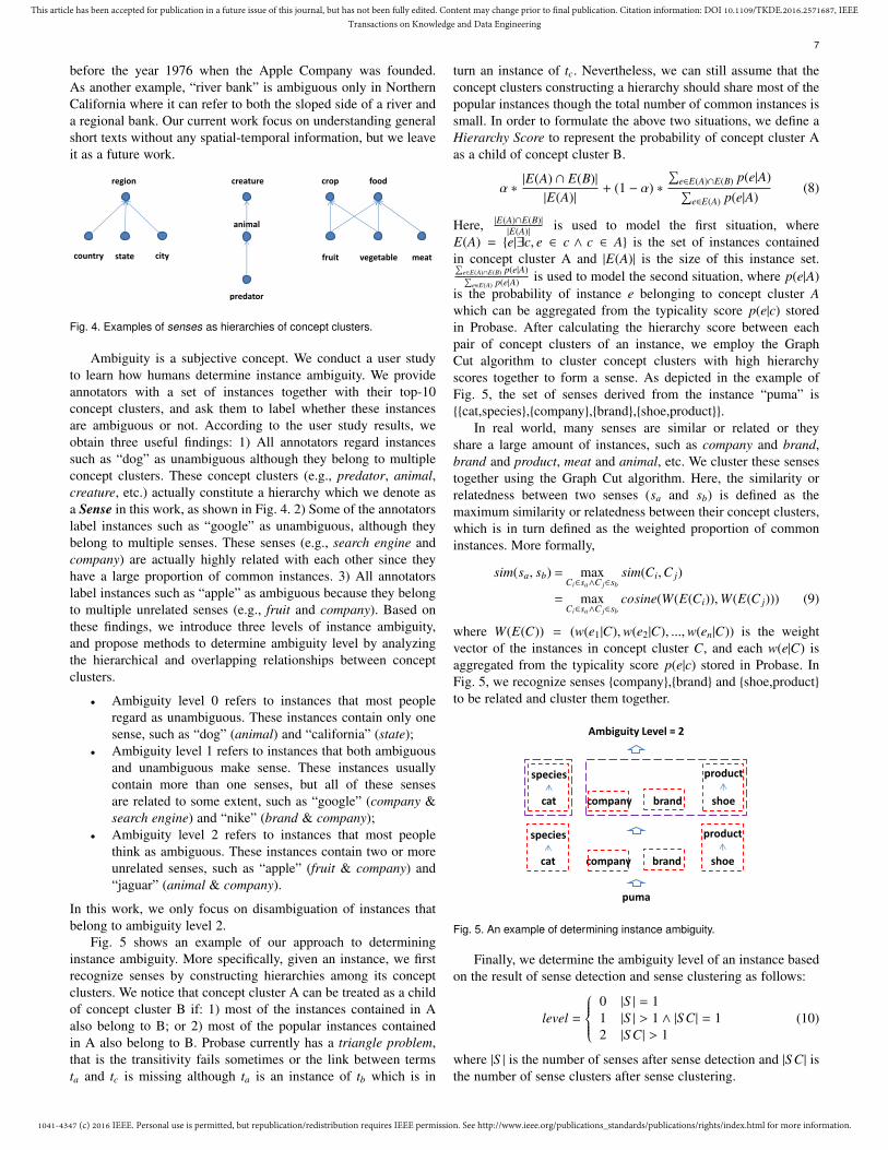
Fig. 5 shows an example of our approach to determininginstance ambiguity. More specifically, given an instance, we firstrecognize senses by constructing hierarchies among its conceptclusters. We notice that concept cluster A can be treated as a childof concept cluster B if: 1) most of the instances contained in Aalso belong to B; or 2) most of the popular instances containedin A also belong to B. Probase currently has a triangle problem,that is the transitivity fails sometimes or the link between termsta and tc is missing although ta is an instance of tb which is in

turn an instance of tc. Nevertheless, we can still assume that theconcept clusters constructing a hierarchy should share most of thepopular instances though the total number of common instances issmall. In order to formulate the above two situations, we define aHierarchy Score to represent the probability of concept cluster Aas a child of concept cluster B.

α ∗|E(A) ∩ E(B)||E(A)|

+ (1 − α) ∗∑

e∈E(A)∩E(B) p(e|A)∑e∈E(A) p(e|A)

(8)

Here, |E(A)∩E(B)||E(A)| is used to model the first situation, where

E(A) = {e|∃c, e ∈ c ∧ c ∈ A} is the set of instances containedin concept cluster A and |E(A)| is the size of this instance set.∑

e∈E(A)∩E(B) p(e|A)∑e∈E(A) p(e|A) is used to model the second situation, where p(e|A)

is the probability of instance e belonging to concept cluster Awhich can be aggregated from the typicality score p(e|c) storedin Probase. After calculating the hierarchy score between eachpair of concept clusters of an instance, we employ the GraphCut algorithm to cluster concept clusters with high hierarchyscores together to form a sense. As depicted in the example ofFig. 5, the set of senses derived from the instance “puma” is{{cat,species},{company},{brand},{shoe,product}}.

In real world, many senses are similar or related or theyshare a large amount of instances, such as company and brand,brand and product, meat and animal, etc. We cluster these sensestogether using the Graph Cut algorithm. Here, the similarity orrelatedness between two senses (sa and sb) is defined as themaximum similarity or relatedness between their concept clusters,which is in turn defined as the weighted proportion of commoninstances. More formally,

sim(sa, sb) = maxCi∈sa∧C j∈sb

sim(Ci,C j)

= maxCi∈sa∧C j∈sb

cosine(W(E(Ci)),W(E(C j))) (9)

where W(E(C)) = (w(e1|C),w(e2|C), ...,w(en|C)) is the weightvector of the instances in concept cluster C, and each w(e|C) isaggregated from the typicality score p(e|c) stored in Probase. InFig. 5, we recognize senses {company},{brand} and {shoe,product}to be related and cluster them together.

puma

species

companycat brand shoe

product

Ambiguity Level = 2

species

companycat brand shoe

product

Fig. 5. An example of determining instance ambiguity.

Finally, we determine the ambiguity level of an instance basedon the result of sense detection and sense clustering as follows:

level =

0 |S | = 11 |S | > 1 ∧ |S C| = 12 |S C| > 1

(10)

where |S | is the number of senses after sense detection and |S C| isthe number of sense clusters after sense clustering.



8

4.2 Online Processing

There are basically three tasks in online processing of short texts,namely text segmentation, type detection, and concept labeling.

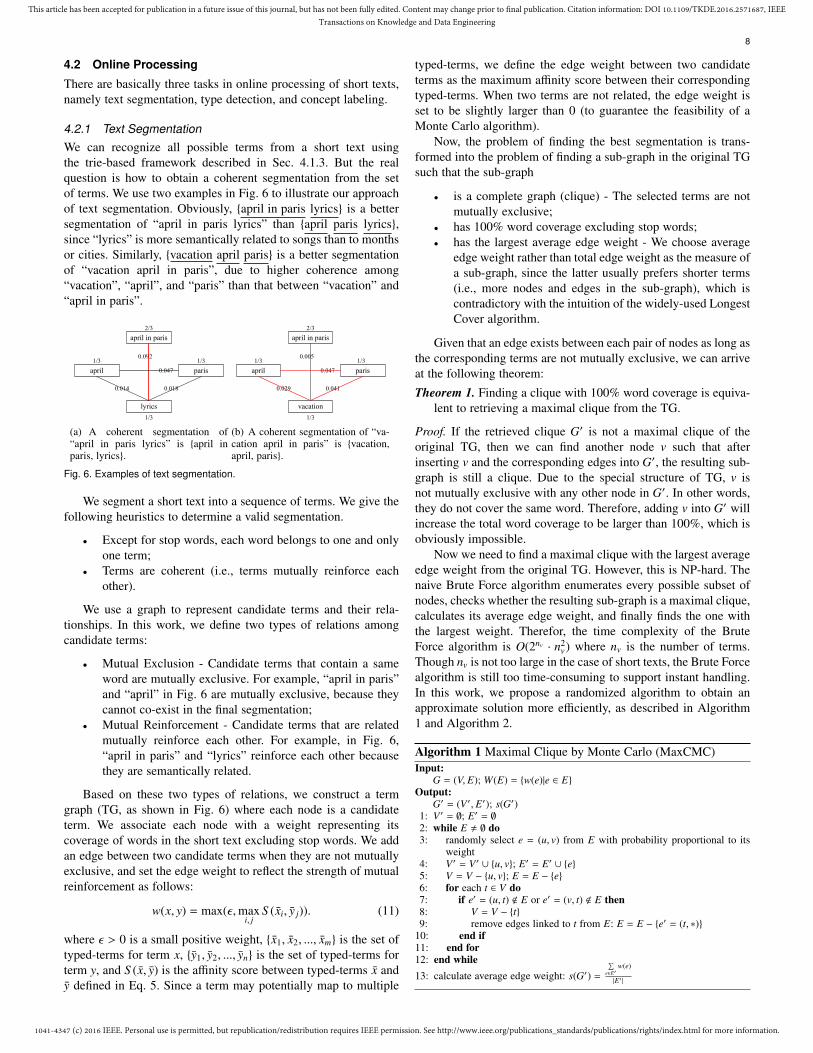
4.2.1 Text SegmentationWe can recognize all possible terms from a short text usingthe trie-based framework described in Sec. 4.1.3. But the realquestion is how to obtain a coherent segmentation from the setof terms. We use two examples in Fig. 6 to illustrate our approachof text segmentation. Obviously, {april in paris lyrics} is a bettersegmentation of “april in paris lyrics” than {april paris lyrics},since “lyrics” is more semantically related to songs than to monthsor cities. Similarly, {vacation april paris} is a better segmentationof “vacation april in paris”, due to higher coherence among“vacation”, “april”, and “paris” than that between “vacation” and“april in paris”.

april in paris

april paris

lyrics

2/3

1/3 1/3

1/3

0.092

0.014 0.018

0.047

(a) A coherent segmentation of“april in paris lyrics” is {april inparis, lyrics}.

april in paris

april paris

vacation

2/3

1/3 1/3

1/3

0.005

0.029 0.041

0.047

(b) A coherent segmentation of “va-cation april in paris” is {vacation,april, paris}.

Fig. 6. Examples of text segmentation.

We segment a short text into a sequence of terms. We give thefollowing heuristics to determine a valid segmentation.

• Except for stop words, each word belongs to one and onlyone term;

• Terms are coherent (i.e., terms mutually reinforce eachother).

We use a graph to represent candidate terms and their rela-tionships. In this work, we define two types of relations amongcandidate terms:

• Mutual Exclusion - Candidate terms that contain a sameword are mutually exclusive. For example, “april in paris”and “april” in Fig. 6 are mutually exclusive, because theycannot co-exist in the final segmentation;

• Mutual Reinforcement - Candidate terms that are relatedmutually reinforce each other. For example, in Fig. 6,“april in paris” and “lyrics” reinforce each other becausethey are semantically related.

Based on these two types of relations, we construct a termgraph (TG, as shown in Fig. 6) where each node is a candidateterm. We associate each node with a weight representing itscoverage of words in the short text excluding stop words. We addan edge between two candidate terms when they are not mutuallyexclusive, and set the edge weight to reflect the strength of mutualreinforcement as follows:

w(x, y) = max(ε,maxi, j

S (xi, y j)). (11)

where ε > 0 is a small positive weight, {x1, x2, ..., xm} is the set oftyped-terms for term x, {y1, y2, ..., yn} is the set of typed-terms forterm y, and S (x, y) is the affinity score between typed-terms x andy defined in Eq. 5. Since a term may potentially map to multiple

typed-terms, we define the edge weight between two candidateterms as the maximum affinity score between their correspondingtyped-terms. When two terms are not related, the edge weight isset to be slightly larger than 0 (to guarantee the feasibility of aMonte Carlo algorithm).

Now, the problem of finding the best segmentation is trans-formed into the problem of finding a sub-graph in the original TGsuch that the sub-graph

• is a complete graph (clique) - The selected terms are notmutually exclusive;

• has 100% word coverage excluding stop words;• has the largest average edge weight - We choose average

edge weight rather than total edge weight as the measure ofa sub-graph, since the latter usually prefers shorter terms(i.e., more nodes and edges in the sub-graph), which iscontradictory with the intuition of the widely-used LongestCover algorithm.

Given that an edge exists between each pair of nodes as long asthe corresponding terms are not mutually exclusive, we can arriveat the following theorem:

Theorem 1. Finding a clique with 100% word coverage is equiva-lent to retrieving a maximal clique from the TG.

Proof. If the retrieved clique G′ is not a maximal clique of theoriginal TG, then we can find another node v such that afterinserting v and the corresponding edges into G′, the resulting sub-graph is still a clique. Due to the special structure of TG, v isnot mutually exclusive with any other node in G′. In other words,they do not cover the same word. Therefore, adding v into G′ willincrease the total word coverage to be larger than 100%, which isobviously impossible.

Now we need to find a maximal clique with the largest averageedge weight from the original TG. However, this is NP-hard. Thenaive Brute Force algorithm enumerates every possible subset ofnodes, checks whether the resulting sub-graph is a maximal clique,calculates its average edge weight, and finally finds the one withthe largest weight. Therefor, the time complexity of the BruteForce algorithm is O(2nv · n2

v) where nv is the number of terms.Though nv is not too large in the case of short texts, the Brute Forcealgorithm is still too time-consuming to support instant handling.In this work, we propose a randomized algorithm to obtain anapproximate solution more efficiently, as described in Algorithm1 and Algorithm 2.

Algorithm 1 Maximal Clique by Monte Carlo (MaxCMC)Input:

G = (V, E); W(E) = {w(e)|e ∈ E}Output:

G′ = (V ′, E′); s(G′)1: V ′ = ∅; E′ = ∅2: while E , ∅ do3: randomly select e = (u, v) from E with probability proportional to its

weight4: V ′ = V ′ ∪ {u, v}; E′ = E′ ∪ {e}5: V = V − {u, v}; E = E − {e}6: for each t ∈ V do7: if e′ = (u, t) < E or e′ = (v, t) < E then8: V = V − {t}9: remove edges linked to t from E: E = E − {e′ = (t, ∗)}

10: end if11: end for12: end while13: calculate average edge weight: s(G′) =

∑e∈E′

w(e)

|E′ |



9

Algorithm 2 Chunking by Maximal Clique (CMaxC)Input:

G = (V, E); W(E) = {w(e)|e ∈ E}number of times to run Algorithm 1: k

Output:G′best = (V ′best, E

′best)

1: smax = 02: for i = 1; i ≤ k; i + + do3: run Algorithm 1 with ¡G′i = (V ′i , E

′i ),s(G′i )¿ as output

4: if s(G′i ) > smax then5: G′best = G′i ; smax = s(G′i )6: end if7: end for

Algorithm 1 runs as follows: First, it randomly selects an edgee = (u, v) with probability proportional to its weight. In otherwords, the larger the edge weight, the higher the probability tobe selected. After picking an edge, it removes all nodes that aredisconnected (namely mutually exclusive) with the picked nodesu or v. At the same time, it removes all edges that are linked tothe deleted nodes. This process is repeated until no edges can beselected. The obtained sub-graph G′ is obviously a maximal cliqueof the original TG. Finally, it evaluates G′ and assigns it with ascore representing the average edge weight. In order to improvethe accuracy of the above algorithm, we repeat it for k times,and choose the maximal clique with the highest score as the finalsegmentation.

In Algorithm 1, the while loop will be repeated for at mostne times, since each time the algorithm removes at least one edgefrom the original TG. Here, ne is the total number of edges inTG. Similarly, the for loop in each while loop will be repeatedfor at most nv times. Therefore, the total time complexity of thisrandomized algorithm is O(k ·ne ·nv) or O(k ·n3

v). Our experimentalresults in Sec. 5 verify the effectiveness and efficiency of thisrandomized algorithm.

4.2.2 Type Detection

Recall that we can obtain the collection of typed-terms for aterm directly from the vocabulary. For example, term “watch”appears in instance-list, concept-list, as well as verb-list ofour vocabulary, thus the possible typed-terms of “watch” are{watch[c],watch[e],watch[v]}. Analogously, the collections of pos-sible typed-terms for “free” and “movie” are { f ree[ad j], f ree[v]}

and {movie[c],movie[e]} respectively, as illustrated in Fig. 7. Foreach term derived from a short text, type detection determines thebest typed-term from the set of possible typed-terms. In the caseof “watch free movie”, the best typed-terms for “watch”, “free”,and “movie” are watch[v], free[ad j], and movie[c] respectively.

The Chain Model

Recall that traditional approaches to POS tagging consider lexicalfeatures only. Most of them adopt Markov Model [23] [24] [25][26] [27] [28] [29] which learns lexical probabilities (P(tag|word))as well as sequential probabilities (P(tagi|tagi−1, ..., tagi−n)) from alabeled corpora of sentences, and tags a new sentence by search-ing for tag sequence that maximizes the combination of lexicaland sequential probabilities. However, such surface features areinsufficient to determine types of terms in the case of short texts.As we have discussed in Challenge 3, “pink” in “pink songs” willbe mistakenly recognized as an adjective using traditional POStaggers, since both the probability of “pink” as an adjective andthat of an adjective preceding a noun are relatively high. Whereas,

“pink” is actually a famous singer and thus should be labeled asan instance, considering the fact that the concept song is muchmore semantically related with the concept singer than the color-describing adjective “pink”. Furthermore, the sequential feature(P(tagi|tagi−1, ..., tagi−n)) fails in short texts. In other words, thetype of a term does not necessarily depend on types of precedingterms only. Therefore, better approaches should be invented toimprove the accuracy of type detection.

Our intuition is that although lexical features are insufficientto determine types of terms derived from a short text, errors canbe reduced substantially by taking into consideration semanticrelations with surrounding context. We believe that the preferredresult of type detection is a sequence of typed-terms whereeach typed-term has a high prior score obtained by consideringtraditional lexical features, and typed-terms in a short text aresemantically coherent with each other.

More formally, we define Singleton Score (SS) to measurethe correctness of a typed-term considering lexical features. Tosimplify implementation, we calculate singleton scores directlybased on the results of traditional POS taggers. Specifically, wefirst obtain the POS tagging result of a short text using anopen source POS tagger - Stanford Tagger7. Then we assignsingleton scores to terms by comparing their types and POS tags.Specifically, terms whose types are consistent with their POStags will get a slightly larger singleton score than those whosetypes are different from their POS tags. Since traditional POStagging methods cannot distinguish among attributes, concepts,and instances, we treat all of them as nouns. This guarantees typesand POS tags to be comparable.

S sg(x) =

{1 + θ x.r = pos(x)1 otherwise (12)

In Eq. 12, x.r and pos(x) are the type and POS tag of typed-termx respectively.

Based on singleton score which represents lexical features oftyped-terms and affinity score which models semantic coherencebetween typed-terms, we formulate the problem of type detectioninto a graph model - the Chain Model. Fig. 7 (a) illustrates anexample of the Chain Model.

We borrow the idea of first order bilexical grammar, andconsider topical coherence between adjacent typed-terms, namelythe preceding and the following one. In particular, we build achain-like graph where nodes are typed-terms retrieved from theoriginal short text, edges are added between each pair of typed-terms mapped from adjacent terms, and the edge weight betweentyped-terms x and y is calculated by multiplying the affinity scorewith the corresponding singleton scores.

w(x, y) = S sg(x) · S (x, y) · S sg(y) (13)

Here, S sg(x) is the singleton score of typed-term x defined in Eq.12, and S (x, y) is the affinity score between typed-terms x and ydefined in Eq. 5.

Now the problem of type detection is transformed into findingthe best sequence of typed-terms collectively, which maximizesthe total weight of the resulting sub-graph. That is, given asequence of terms {t1, t2, ..., tl} derived from the original short

7. http://nlp.stanford.edu/software/tagger.shtml



10

text, we need to find a corresponding sequence of typed-terms{t∗1, t

∗2, ..., t

∗l } that maximize:

l−1∑i=1

w(ti, ti+1) (14)

In the case of “watch free movie”, the best se-quence of typed-terms detected using the Chain Model is{watch[e], f ree[ad j],movie[c]}, as illustrated in Fig. 7 (a).

watch[c]

watch[e]

watch[v]

watch

free[adj]

free[v]

movie[c]

movie[e]

free

movie

(a) Type detection result of “watchfree movie using the Chain Modelis {watch[e], f ree[ad j], movie[c]}.

watch[c]

watch[e]

watch[v]

watch

free[adj]

free[v]

movie[c]

movie[e]

free

movie

(b) Type detection result of “watchfree movie using the PairwiseModel is {watch[v], f ree[ad j],movie[c]}.

Fig. 7. Difference between Chain Model and Pairwise Model.

The Pairwise ModelIn fact, terms that are most related in a short text might notalways be adjacent. Therefore, if we only consider semanticrelations between consecutive terms, like in the Chain Model, itwill lead to mistakes. In the case of “watch free movie” in Fig.7 (a), the Chain Model incorrectly recognizes “watch” to be aninstance, since “watch” is an instance of the concept product inour knowledgebase, and the probability of adjective “free” co-occurring with concept product is relatively high. However, whenrelatedness between “watch” and “movie” is considered, “watch”should be labeled as a verb. The Pairwise Model is able to capturesuch cross-term relations. More specifically, the Pairwise Modeladds edges between typed-terms mapped from each pair of termsrather than adjacent terms only. In Fig. 7 (b), there are edgesbetween nonadjacent terms “watch” and “movie”, in addition tothose between “watch” and “free” as well as those between “free”and “movie”.

Like the assumption of Chain Model, the best sequence oftyped-terms should be semantically coherent. One thing to note isthat although cross-term relations are considered in the Pairwisemodel, a typed-term is not required to be related with every othertyped-term. Instead, we assume that it should be semantically co-herent with at least one other typed-term. Therefore, the goal of thePairwise Model is to find the best sequence of typed-terms whichguarantees that the maximum spanning tree (MST) of the resultingsub-graph has the largest weight. In Fig. 7 (b), as long as the totalweight of edge between watch[v] and movie[c] and that betweenf ree[ad j] and movie[c] is the largest, {watch[v], f ree[ad j],movie[c]}

can be successfully recognized as the best sequence of typed-terms for “watch free movie”, in regardless of relations betweenwatch[v] and f ree[ad j].

We employ the Pairwise Model in our prototype system as theapproach to type detection. But we present the accuracy of bothmodels in the experiments, in order to verify the superiority ofPairwise Model over Chain Model.

4.2.3 Concept LabelingThe most important task in concept labeling is instance dis-ambiguation, which is the process of eliminating inappropriate

semantics behind an ambiguous instance. We accomplish this taskby re-ranking concept clusters of the target instance based oncontext information in a short text (i.e., remaining terms), so thatthe most appropriate concept clusters are ranked higher and theincorrect ones lower.

Our intuition is that a concept cluster is appropriate for aninstance only if it is a common semantics of that instance and itachieves support from surrounding context at the same time. Take“hotel california eagles” as an example. Although both animal andmusic band are popular semantics of “eagles”, only music band issemantically coherent (i.e., frequently co-occurs) with the conceptsong and thus can be kept as the final semantics of “eagles”.

We have mentioned before that a term is not necessarily relatedwith every other term in the short text. If irrelevant terms areused to disambiguate a target instance, most of its concept clusterswill obtain little support, which will in turn lead to over-filtering.Therefore, we decide to use only the most related term to helpwith disambiguation. In the Chain Model and Pairwise Model,we have obtained the best sequence of typed-terms together withthe weighted edges in-between, hence the most related term canbe retrieved straightforwardly by comparing weights of edgesconnecting to the target instance.

Based on the aforementioned intuition, we model the processof instance disambiguation using a Weighted Vote approach. As-sume that the target ambiguous instance is x whose concept clustervector is x. ~C = (〈C1,W1〉, ..., 〈CN ,WN〉), and the most relatedtyped-term used for disambiguation is y. Then the importance ofeach concept cluster in x’s disambiguated concept cluster vectorx. ~C′ = (〈C1,W ′1〉, ..., 〈CN ,W ′N〉) is a combination of self-vote andcontext-vote. More formally,

x.W ′i = Vsel f (Ci) · Vcontext(Ci) (15)

Here, self-vote Vsel f (Ci) represents the original weight of conceptcluster Ci obtained from Probase, namely Vsel f (Ci) = x.Wi;context-vote Vcontext(Ci) represents the probability of Ci as aco-occurrence neighbor of the context y. In other words, self-vote Vsel f (Ci) can be calculated using Eq. 1, and context-voteVcontext(Ci) is the weight of Ci in y’s co-occur concept clustervector which can be retrieved directly from the compressed co-occurrence network described in Sec. 4.1.1.

In the case of “hotel california eagles”, the original con-cept cluster vector of “eagles” is (〈animal,0.2379〉,〈band,0.1277〉,〈bird,0.1101〉,〈celebrity,0.0463〉...) and the co-occur concept clus-ter vector of context term “hotel california” is (〈singer,0.0237〉,〈band,0.0181〉, 〈celebrity,0.0137〉, 〈album,0.0132〉...). After dis-ambiguation using Weighted Vote, the final concept clus-ter vector of “eagles” (after normalization) is (〈band,0.4562〉,〈celebrity,0.1583〉,〈animal,0.1317〉,〈singer,0.0911〉...).

5 ExperimentWe conducted comprehensive experiments on real-world datasetsto evaluate the performance of our approach to short text under-standing. All the algorithms were implemented in C#, and all theexperiments were conducted on a server with 2.90GHz Intel XeonE5-2690 CPU and 192GB memory.

5.1 Benchmark

One of the most notable contributions in this work is that webuild a generalized framework for short text understanding whichcan recognize best segmentations, conduct type detection, and



11

eliminate instance ambiguity explicitly based on various typesof context information. Therefore, we manually picked 11 am-biguous terms (i.e., “april in paris” and “hotel california” withsegmentation ambiguity; “watch”, “book”, “pink”, “blue”, “or-ange”, “population”, and “birthday” with type ambiguity; “apple”and “fox” with instance ambiguity) and randomly selected 1100queries containing one of these terms from one day’s querylog(100 queries for each term) to check the performance of ourframework for disambiguation. Furthermore, in order to examinethe performance of our system on general queries, we randomlysampled another 400 queries without any restriction. Based onthese queries, we constructed three testing datasets:

• ambig - queries containing ambiguous terms;• general - general queries;• all - all queries in our query dataset;

To verify the generalizability of our framework on other shorttexts, we randomly sampled 1500 tweets using Twitter’s API.We preprocessed the tweet dataset by removing some tweet-specific features, such as @username, hashtags, urls, etc., andother noise, such as words containing more than three continuoussame characters (e.g., “Oooooooops”). We divided each datasetinto 5 disjoint parts, and invited 15 colleagues to label them (3 foreach part). Final labels were based on majority vote.

5.2 Effectiveness

5.2.1 Effectiveness of Text Segmentation

One prerequisite to text segmentation is to locate candidate terms.In order to cope with the noise in short texts, we constructa large-scale vocabulary which incorporates terms as well astheir abbreviations and nicknames. Furthermore, we adopt andextend the trie-based method [37] to allow for approximate termextraction with varying edit distance constraints. We compare theperformance of our approach (i.e., Trie with Varying edit distance,TrieV) with the trie-based method (i.e., Trie) and exact matchingmethod (i.e., Exact), in terms of precision, recall, and f1-measure.From Table 2 we can see that approximate term extraction canobtain more terms from short texts than exact matching, at thecost of introducing slightly more extraction errors. By allowing forvarious edit distance thresholds depending on text length, TrieVimproves the precision of Trie by reducing extraction errors causedby short terms, abbreviations, etc. Overall, TrieV achieves thehighest f1-measure in both datasets. Note that the performanceof all these term extraction methods is consistently better in thequery dataset than in the tweet dataset. This is mainly becausetweets are usually more informal and noisy than queries.

TABLE 2Performance of term extraction.

precision recall f1-measure

queryExact 0.988 0.847 0.912Trie 0.943 0.922 0.932

TrieV 0.984 0.918 0.950

tweetExact 0.980 0.718 0.829Trie 0.938 0.847 0.890

TrieV 0.972 0.833 0.897

Given the set of candidate terms extracted from a short text,we construct a term graph (TG) between candidate terms andconduct segmentation by searching for the maximal clique with

the largest average edge weight in TG. We propose a randomizedalgorithm to reduce time cost of the naive Brute Force algorithm.Therefore, we compare the precision of three models for textsegmentation, namely Longest Cover, MaxCBF (Maximal Cliqueby Brute Force) and MaxCMC (Maximal Clique by Monte Carlo).From the results in Table 3 we can see that the Maximal Cliqueapproach to text segmentation achieves better performance thanthe Longest Cover algorithm by taking into consideration contextsemantics in addition to traditional surface features like length.Furthermore, the randomized algorithm designed to improve ef-ficiency also achieves comparable precision to that of the BruteForce search. We can also observe that the precision improvementof our approaches over the Longest Cover method is much largerfor ambiguous queries (7.5% in “ambig” dataset) than generalqueries (1.8% in “general” dataset), which is consistent with ourexpectation.

TABLE 3Precision of text segmentation.

Longest Cover MaxCBF MaxCMC

queryambig 0.905 0.980 0.970general 0.972 0.990 0.982

all 0.954 0.984 0.979tweet 0.961 0.980 0.973

5.2.2 Effectiveness of Type DetectionIn this part, we compare our approaches to type detection (i.e.,the Chain Model and Pairwise Model) with a widely-used, non-commercial POS tagger - Stanford Tagger. Since traditional POStaggers do not distinguish among attributes, concepts and in-stances, we need to address this problem first in order to make areasonable comparison. We consider two situations here: 1) if therecognized term contains multiple words or its POS tag is noun,then we check the frequency of that term as an attribute, a conceptand an instance respectively in our knowledgebase, and choose thetype with the highest frequency as its label; 2) otherwise, we labelthe term according to its POS tag.

Table 4 demonstrates the precision of Stanford Tagger (ST),Chain Model (CM) and Pairwise Model (PM) for type detection.We use four kinds of precision to measure the effectiveness ofthese models:

• lexical-level: the percentage of correct lexical (i.e., verband adjective) term-type pairs;

• semantic-level: the percentage of correct semantic (i.e.,attribute, concept and instance) term-type pairs;

• term-level: the percentage of correct term-type pairs;• text-level: the percentage of short texts whose term-type

pairs are all correct.

The results of lexical-level, semantic-level, and term-level preci-sion in the three query datasets (i.e., “ambig”, “general”, and “all”)illustrate similar trends with text-level precision. Therefore, weonly present the differences at text level. For the other three levelsof precision, we present results for the “all” query dataset. FromTable 4, we can see that the Pairwise Model performs better thanthe Chain Model on all kinds of precision measures, which in turnprovides better precision than the Stanford Tagger in both querydataset and tweet dataset. However, the precision improvement isslightly larger in the query data set than in the tweet dataset. Thisis mainly because tweets are more grammatically structured than



12

keyword queries, making traditional POS tagging more reliable.Interestingly, the lexical-level precision of the Chain Model andthe Pairwise Model is also larger than traditional POS taggers.Since the Stanford Tagger only pays attention to lexical features, itwill mistakenly recognize “pink” in “pink songs” as an adjective,which is actually an instance of singer. The Chain Model andPairwise Model, on the contrary, take context semantics intoconsideration and thus can solve the above problem. The ChainModel has the limitation that it only considers semantic relationsbetween adjacent terms, which makes it incomparable with thePairwise Model. Note that the precision improvement of the Pair-wise Model over Stanford Tagger is much larger for ambiguousqueries (12.3% in “ambig” dataset) than general queries (7.5%in “general” dataset), which further verifies the superiority of ourapproach to reduce ambiguity in type detection.

TABLE 4Precision of type detection.

ST CM PM

query

lexical-level 0.865 0.967 0.978semantic-level 0.944 0.969 0.973

term-level 0.932 0.968 0.974

text-levelambig 0.837 0.945 0.960general 0.902 0.962 0.977

all 0.876 0.955 0.967

tweet

lexical-level 0.962 0.965 0.984semantic-level 0.950 0.970 0.977

term-level 0.944 0.963 0.980text-level 0.891 0.958 0.968

Recall that we employ a singleton score to incorporate theresult of traditional POS taggers in the Chain Model and PairwiseModel. We assign singleton score of a typed-term as 1 + θ whenits type is consistent with its POS tag, and 1 otherwise. In otherwords, the variable θ represents the amount of impact lexicalfeatures have on type detection results. Fig. 8 depicts the variationof type detection precision on terms and short texts, when θ rangesfrom 0 to 1. We can see that the precision of type detectionincreases dramatically when context semantics and lexical featuresare combined to estimate best types (from θ = 0 to θ = 0.1).However, as lexical features play an increasingly important rolein the Chain Model and Pairwise Model, the precision decreasesslightly (from θ = 0.2 to θ = 1). Most notably, the precisionof type detection using Chain Model and Pairwise Model whenθ = 0 (namely only semantic features are considered) is largerthan that of the Standford Parser depicted in Table 4. This provesthat context semantics are more important than lexical features fordetermining types of terms in short texts.

0.93

0.94

0.95

0.96

0.97

0.98

0.99

1

0 0.1 0.2 0.3 0.4 0.5 0.6 0.7 0.8 0.9 1

Pre

cisi

on

θ

query-termquery-texttweet-termtweet-text

(a) Chain Model.

0.95

0.96

0.97

0.98

0.99

1

0 0.1 0.2 0.3 0.4 0.5 0.6 0.7 0.8 0.9 1

Pre

cisi

on

θ

query-termquery-texttweet-termtweet-text

(b) Pairwise Model.

Fig. 8. Precision of type detection when θ increases.

5.2.3 Effectiveness of Short Text UnderstandingOne of the most notable contributions of our work is that wepropose a generalized framework that can recognize best segmen-tations, conduct type detection, and eliminate instance ambiguitybased on various types of context information. Therefore, weexamine the effectiveness of short text understanding as a wholein this part. More specifically, we compare the performance ofour framework with current state-of-the-art approaches to miningsemantics from short texts, namely [16] which conducts instancedisambiguation in queries based on similar instances, [17] whichconducts instance disambiguation in queries based on relatedinstances, and [15] which conducts instance disambiguation intweets based on both similar and related instances. As before, weconsider both term-level and text-level precisions to measure theeffectiveness of short text understanding. We present the results inthe three query datasets (i.e., “ambig”, “general”, and “all”) onlyat text level. For term-level precision, we present results achievedin the “all” query dataset. From Table 5 we can see that ourapproach performs dramatically better than current state-of-the-artapproaches, since it can utilize various context information to con-duct instance disambiguation. Note that the precision improvementof our framework over existing state-of-the-art methods is onlyslightly larger for ambiguous queries (38.1% in “ambig” dataset)than general queries (35.3% in “general” dataset), since manygeneral queries also contain ambiguous instances. We observe329 out of 517 instances (63.6%) derived from the “general”query dataset are ambiguous. Another interesting finding is thatour framework improves precision to a larger extent in the querydataset (36.4%) than in the tweet dataset (12%). This can beexplained from two aspects: first, tweets are usually longer thankeyword queries, providing more context information for instancedisambiguation; second, [15] disambiguates instances based onboth similar instances and related instances. These two featurescontribute to more accurate semantic interpretations of short textsusing [15] than those obtained using [16] or [17], which in turnresults in smaller precision improvement in the tweet dataset thanin the query dataset. Overall, our framework achieves not onlyhigh but also comparable precision of short text understanding inboth datasets (89.0% in query dataset and 89.4% in tweet dataset),which verifies its effectiveness and robustness.

TABLE 5Precision of short text understanding.

[16] [17] [15] Our

query

term-level 0.694 0.701 - 0.943

text-levelambig 0.487 0.503 - 0.884general 0.556 0.556 - 0.909

all 0.525 0.526 - 0.890

tweet term-level - - 0.841 0.922text-level - - 0.774 0.894

In Sec. 4.1.4, we described how to determine whether aninstance is ambiguous or not based on its semantics (i.e., conceptclusters). Specifically, we group concept clusters into senses (i.e.,hierarchies of concept clusters), cluster similar or related sensesinto sense clusters, and then determine instance ambiguity levelaccording to the number of sense clusters, as illustrated in Fig.5. To examine the performance of this method, we randomlysampled 900 instances (300 from each ambiguity level), andinvited colleagues to label their ambiguity with three options:“ambiguous”, “unambiguous”, and “hard to say”. We observe



13

that our algorithm agrees with human annotators for most ofthe instances (82.2% agreement), and the disagreement mainlyhappens in instances from ambiguity level 1 (41% disagreement).In Equation 8, we combine two conditions that can indicate thehierarchical relationship between two concept clusters, namely thepercentage of common instances and common popular instances,using a parameter α. We demonstrate how the choice of α influ-ences the precision of ambiguity detection in Fig. 9 (a). We cansee that the percentage of common popular instances (i.e., α = 0)contributes more to estimating hierarchical relationship than thepercentage of common instances (i.e., α = 1). This is mainlydue to the triangle problem in Probase. We determine instanceambiguity in this work for two reasons. First, it is obvious that thetime cost of short text understanding can be reduced by skippingunambiguous instances when conducting instance disambiguation.Second, disambiguating unambiguous instances will cause over-filtering sometimes, which in turn affects the accuracy of shorttext understanding, as verified in Fig. 9 (b).

0.5

0.55

0.6

0.65

0.7

0.75

0.8

0.85

0.9

0.95

1

0 0.1 0.2 0.3 0.4 0.5 0.6 0.7 0.8 0.9 1

Pre

cis

ion

α

(a) Precision of instance ambiguitydetection when α increases.

0.7

0.75

0.8

0.85

0.9

0.95

1

Query Tweet

Pre

cisi

on

with ambiguitywithout ambiguity

(b) Impact of instance ambiguity de-tection on short text understanding.

Fig. 9. Effectiveness of instance ambiguity detection.

5.3 Efficiency

As we know, short text understanding is usually regarded as anonline task or an underlying step of many other text miningapplications like classification and clustering. These applicationsusually need to handle millions of short texts at a time, whichmakes the efficiency of short text understanding extremely critical.Therefore, we examine the time requirement of our framework toverify its efficiency, as depicted in Fig. 10 (a). We can see that ourframework can efficiently interpret a short text within hundreds ofmilliseconds, and the time requirement increases linearly with theascending of text length. Note that the time required to handle atweet is mostly shorter than that required to handle a query of thesame length. One possible explanation is that a large proportion ofwords in tweets are stopwords which need little processing, whilewords in queries are mostly keywords. In Sec. 4.2.1, we describeda randomized algorithm (MaxCMC) to reduce the time cost ofthe Brute Force algorithm (MaxCBF) for text segmentation. Wedepict the average time requirement of these two methods for textsegmentation in Fig. 10 (b). The average time requirement of textsegmentation is consistently larger in tweets than in queries, sincetweets contain more words than queries in average.

6 ConclusionIn this work, we propose a generalized framework to understandshort texts effectively and efficiently. More specifically, we dividethe task of short text understanding into three subtasks: textsegmentation, type detection, and concept labeling. We formu-late text segmentation as a weighted Maximal Clique problem,and propose a randomized approximation algorithm to maintain

0

50

100

150

200

250

300

1 2 3 4 5 6 7 8 9 10 11 12 13 14 15

Tim

e (m

s)

Text Length

TweetQuery

(a) Average time cost of our frame-work when text length increases.

0

20

40

60

80

100

Query Tweet

Tim

e (m

s)

randomizedbrute force

(b) Efficiency improvement of therandomized algorithm.

Fig. 10. Efficiency.

accuracy and improve efficiency at the same time. We introducea Chain Model and a Pairwise Model which combine lexicaland semantic features to conduct type detection. They achievebetter accuracy than traditional POS taggers on the labeled bench-mark. We employ a Weighted Vote algorithm to determine themost appropriate semantics for an instance when ambiguity isdetected. The experimental results demonstrate that our proposedframework outperforms existing state-of-the-art approaches in thefield of short text understanding. As a future work, we attemptto analyze and incorporate the impact of spatial-temporal featuresinto our framework for short text understanding.

AcknowledgmentsThis work was partially supported by the National 863 High-tech Program under Grant No. 2012AA011001, the National KeyBasic Research Program (973 Program) of China under Grant No.2014CB340403, and the National Natural Science Foundation ofChina under Grant No. M13210007.

References[1] A. McCallum and W. Li, “Early results for named entity recognition with

conditional random fields, feature induction and web-enhanced lexicons,”in Proceedings of the Seventh Conference on Natural Language Learningat HLT-NAACL 2003 - Volume 4, ser. CONLL ’03, Stroudsburg, PA, USA,2003, pp. 188–191.

[2] G. Zhou and J. Su, “Named entity recognition using an hmm-based chunktagger,” in Proceedings of the 40th Annual Meeting on Association forComputational Linguistics, ser. ACL ’02, Stroudsburg, PA, USA, 2002,pp. 473–480.

[3] D. M. Blei, A. Y. Ng, and M. I. Jordan, “Latent dirichlet allocation,” J.Mach. Learn. Res., vol. 3, pp. 993–1022, 2003.

[4] M. Rosen-Zvi, T. Griffiths, M. Steyvers, and P. Smyth, “The author-topicmodel for authors and documents,” in Proceedings of the 20th Conferenceon Uncertainty in Artificial Intelligence, ser. UAI ’04, Arlington, Virginia,United States, 2004, pp. 487–494.

[5] R. Mihalcea and A. Csomai, “Wikify! linking documents to encyclopedicknowledge,” in Proceedings of the sixteenth ACM conference on Confer-ence on information and knowledge management, ser. CIKM ’07, NewYork, NY, USA, 2007, pp. 233–242.

[6] D. Milne and I. H. Witten, “Learning to link with wikipedia,” in Pro-ceedings of the 17th ACM conference on Information and knowledgemanagement, ser. CIKM ’08, New York, NY, USA, 2008, pp. 509–518.

[7] S. Kulkarni, A. Singh, G. Ramakrishnan, and S. Chakrabarti, “Collectiveannotation of wikipedia entities in web text,” in Proceedings of the 15thACM SIGKDD international conference on Knowledge discovery and datamining, ser. KDD ’09, New York, NY, USA, 2009, pp. 457–466.

[8] X. Han and J. Zhao, “Named entity disambiguation by leveragingwikipedia semantic knowledge,” in Proceedings of the 18th ACM con-ference on Information and knowledge management, ser. CIKM ’09, NewYork, NY, USA, 2009, pp. 215–224.

[9] ——, “Structural semantic relatedness: A knowledge-based method tonamed entity disambiguation,” in Proceedings of the 48th Annual Meetingof the Association for Computational Linguistics, ser. ACL ’10, Strouds-burg, PA, USA, 2010, pp. 50–59.



14

[10] X. Han, L. Sun, and J. Zhao, “Collective entity linking in web text:A graph-based method,” in Proceedings of the 34th International ACMSIGIR Conference on Research and Development in Information Retrieval,ser. SIGIR ’11, New York, NY, USA, 2011, pp. 765–774.

[11] W. Shen, J. Wang, P. Luo, and M. Wang, “Linden: Linking named entitieswith knowledge base via semantic knowledge,” in Proceedings of the 21stInternational Conference on World Wide Web, ser. WWW ’12, New York,NY, USA, 2012, pp. 449–458.

[12] G. L. Murphy, The big book of concepts. MIT press, 2004.[13] C. Li, J. Weng, Q. He, Y. Yao, A. Datta, A. Sun, and B.-S. Lee, “Twiner:

Named entity recognition in targeted twitter stream,” in Proceedings of the35th International ACM SIGIR Conference on Research and Developmentin Information Retrieval, ser. SIGIR ’12, New York, NY, USA, 2012, pp.721–730.

[14] D. M. de Oliveira, A. H. Laender, A. Veloso, and A. S. da Silva, “Fs-ner: A lightweight filter-stream approach to named entity recognition ontwitter data,” in Proceedings of the 22nd International Conference onWorld Wide Web, ser. WWW ’13 Companion, Republic and Canton ofGeneva, Switzerland, 2013, pp. 597–604.

[15] P. Ferragina and U. Scaiella, “Tagme: On-the-fly annotation of shorttext fragments (by wikipedia entities),” in Proceedings of the 19th ACMInternational Conference on Information and Knowledge Management,ser. CIKM ’10, New York, NY, USA, 2010, pp. 1625–1628.

[16] Y. Song, H. Wang, Z. Wang, H. Li, and W. Chen, “Short text concep-tualization using a probabilistic knowledgebase,” in Proceedings of theTwenty-Second international joint conference on Artificial Intelligence -Volume Volume Three, ser. IJCAI’11, 2011, pp. 2330–2336.

[17] D. Kim, H. Wang, and A. Oh, “Context-dependent conceptualization,”in Proceedings of the Twenty-Third International Joint Conference onArtificial Intelligence, ser. IJCAI’13, 2013, pp. 2654–2661.

[18] S. Klein and R. F. Simmons, “A computational approach to grammaticalcoding of english words,” J. ACM, vol. 10, no. 3, pp. 334–347, 1963.

[19] B. B. Greene and G. M. Rubin, Automatic grammatical tagging ofEnglish. Department of Linguistics, Brown University, 1971.

[20] E. Brill, “A simple rule-based part of speech tagger,” in Proceedings ofthe workshop on Speech and Natural Language, ser. HLT ’91, Strouds-burg, PA, USA, 1992, pp. 112–116.

[21] E. BRILL, “Some advances in transformation-based part of speechtagging,” in National Conference on Artificial Intelligence, 1994, pp. 722–727.

[22] E. Brill, “Transformation-based error-driven learning and natural lan-guage processing: a case study in part-of-speech tagging,” Comput. Lin-guist., vol. 21, no. 4, pp. 543–565, 1995.

[23] K. W. Church, “A stochastic parts program and noun phrase parser forunrestricted text,” in Proceedings of the second conference on Appliednatural language processing, ser. ANLC ’88, Stroudsburg, PA, USA,1988, pp. 136–143.

[24] S. J. DeRose, “Grammatical category disambiguation by statistical opti-mization,” Comput. Linguist., vol. 14, no. 1, pp. 31–39, 1988.

[25] C. G. de Marcken, “Parsing the lob corpus,” in Proceedings of the 28thannual meeting on Association for Computational Linguistics, ser. ACL’90, Stroudsburg, PA, USA, 1990, pp. 243–251.

[26] D. Cutting, J. Kupiec, J. Pedersen, and P. Sibun, “A practical part-of-speech tagger,” in Proceedings of the third conference on Applied naturallanguage processing, ser. ANLC ’92, Stroudsburg, PA, USA, 1992, pp.133–140.

[27] R. Weischedel, R. Schwartz, J. Palmucci, M. Meteer, and L. Ramshaw,“Coping with ambiguity and unknown words through probabilistic mod-els,” Comput. Linguist., vol. 19, no. 2, pp. 361–382, 1993.

[28] B. Merialdo, “Tagging english text with a probabilistic model,” Comput.Linguist., vol. 20, no. 2, pp. 155–171, 1994.

[29] H. Schutze and Y. Singer, “Part-of-speech tagging using a variablememory markov model,” in Proceedings of the 32nd annual meeting onAssociation for Computational Linguistics, ser. ACL ’94, Stroudsburg, PA,USA, 1994, pp. 181–187.

[30] M. Utiyama and H. Isahara, “A statistical model for domain-independenttext segmentation,” in Proceedings of the 39th Annual Meeting on Associ-ation for Computational Linguistics, ser. ACL ’01, Stroudsburg, PA, USA,2001, pp. 499–506.

[31] N. Mishra, R. Saha Roy, N. Ganguly, S. Laxman, and M. Choudhury,“Unsupervised query segmentation using only query logs,” in Proceedingsof the 20th International Conference Companion on World Wide Web, ser.WWW ’11, 2011, pp. 91–92.

[32] M. Hagen, M. Potthast, B. Stein, and C. Brautigam, “Query segmentationrevisited,” in Proceedings of the 20th International Conference on WorldWide Web, ser. WWW ’11, New York, NY, USA, 2011, pp. 97–106.

[33] W. Wu, H. Li, H. Wang, and K. Q. Zhu, “Probase: a probabilistic taxon-omy for text understanding,” in Proceedings of the 2012 ACM SIGMODInternational Conference on Management of Data, ser. SIGMOD ’12, NewYork, NY, USA, 2012, pp. 481–492.

[34] T. Lee, Z. Wang, H. Wang, and S. won Hwang, “Attribute extraction andscoring: A probabilistic approach,” in Data Engineering (ICDE), 2013IEEE 29th International Conference on, April 2013, pp. 194–205.

[35] L. Kaufman and P. J. Rousseeuw, Finding groups in data: an introductionto cluster analysis. John Wiley & Sons, 2009, vol. 344.

[36] P. Li, H. Wang, K. Q. Zhu, Z. Wang, and X. Wu, “Computing termsimilarity by large probabilistic isa knowledge,” in Proceedings of the22Nd ACM International Conference on Conference on Information&Knowledge Management, ser. CIKM ’13, New York, NY, USA, 2013, pp.1401–1410.

[37] D. Deng, G. Li, and J. Feng, “An efficient trie-based method for approx-imate entity extraction with edit-distance constraints,” in Proceedings ofthe 2012 IEEE 28th International Conference on Data Engineering, ser.ICDE ’12, Washington, DC, USA, 2012, pp. 762–773.

[38] W. Wang, C. Xiao, X. Lin, and C. Zhang, “Efficient approximate entityextraction with edit distance constraints,” in Proceedings of the 2009ACM SIGMOD International Conference on Management of Data, ser.SIGMOD ’09, New York, NY, USA, 2009, pp. 759–770.

[39] G. Li, D. Deng, and J. Feng, “Faerie: Efficient filtering algorithms forapproximate dictionary-based entity extraction,” in Proceedings of the2011 ACM SIGMOD International Conference on Management of Data,ser. SIGMOD ’11, New York, NY, USA, 2011, pp. 529–540.

Wen Hua is currently a Postdoctoral Research Fellow at the Universityof Queensland. She received her bachelor and PhD degrees in computerscience from Renmin University of China in 2010 and 2015 respectively. Herresearch interests include natural language processing, information retrievaland extraction, data mining, social media analysis, and graph management.

Zhongyuan Wang is currently a Researcher at Microsoft Research Asia.He received his bachelor, master, and PhD degrees in computer sciencefrom Renmin University of China in 2007, 2010, and 2015 respectively.His research interests include knowledge base, web data mining, onlineadvertising, machine learning, and natural language processing.

Haixun Wang received the bachelor and master degrees in computerscience from Shanghai Jiao Tong University in 1994 and 1996 respectively,and the PhD degree in computer science from the University of California,Los Angeles in 2000. He joined Google Research, Mountain View in 2013.His research interests include text analytics, natural language processing,knowledge base, semantic network, artificial intelligence, database lan-guage and system, graph data management, etc. He is a member of IEEE.

Kai Zheng is currently an ARC DECRA (Australia Research Council Discov-ery Early Career Researcher Award) Fellow at the University of Queensland.He received his PhD degree in computer science from the University ofQueensland in 2012. His research focus is to find effective and efficientsolutions for managing, integrating and analyzing big data for business,scientific and personal applications. He has been working in the area ofsocial-media analysis, spatial-temporal databases, uncertain databases,data mining and bioinformatics. He has also been appointed as adjunctprofessor in the School of Computer Science at Soochow University since2015. He is a member of IEEE.

Xiaofang Zhou received the bachelor and master degrees in computerscience from Nanjing University in 1984 and 1987 respectively, and the PhDdegree in computer science from the University of Queensland in 1994. Heis a professor of computer science with the University of Queensland. He isthe head of the Data and Knowledge Engineering Research Division, Schoolof Information Technology and Electrical Engineering. He is also an speciallyappointed adjunct professor at Soochow University, China. His research isfocused on finding effective and efficient solutions to managing integrating,and analyzing very large amounts of complex data for business and sci-entific applications. His research interests include spatial and multimediadatabases, high performance query processing, web information systems,data mining, and data quality management. He is a senior member of IEEE.

Documents

Understand Short Texts by Harvesting and Analyzing ... · Compared with documents, short texts are generated in a much larger volume. For example, Google, as the most widely used