Embed Size (px)
Citation preview

Institute of Parallel and Distributed SystemsUniversity of StuttgartUniversitätsstraße 38
D–70569 Stuttgart
Diplomarbeit Nr. 3150
Underlay aware approach tosupport quality of service inpublish-subscribe systems
Christian Schieberle
Course of Study: Software Engineering
Examiner: Prof. Dr. Dr. h. c. Kurt Rothermel
Supervisor: M. Sc. M. Adnan Tariq
Commenced: March 1, 2011
Completed: August 31, 2011
CR-Classification: C.2.4, C.2.2

Contents
1 Abstract 7
2 Introduction 9
3 Related work 113.1 QoS in publish-subscribe systems . . . . . . . . . . . . . . . . . . . . . . . . . . 113.2 QoS in overlays . . . . . . . . . . . . . . . . . . . . . . . . . . . . . . . . . . . . 123.3 Topology inference . . . . . . . . . . . . . . . . . . . . . . . . . . . . . . . . . . 133.4 Approximation algorithms for Minimum Routing Cost Spanning Trees . . . . . . 13
4 System model and problem statement 154.1 System model . . . . . . . . . . . . . . . . . . . . . . . . . . . . . . . . . . . . . 154.2 Problem statement . . . . . . . . . . . . . . . . . . . . . . . . . . . . . . . . . . 18
5 Approach overview 19
6 Topology discovery 236.1 Prefixes . . . . . . . . . . . . . . . . . . . . . . . . . . . . . . . . . . . . . . . . 246.2 Joining the overlay . . . . . . . . . . . . . . . . . . . . . . . . . . . . . . . . . . 256.3 Limited flooding strategy . . . . . . . . . . . . . . . . . . . . . . . . . . . . . . . 276.4 Random walk strategy . . . . . . . . . . . . . . . . . . . . . . . . . . . . . . . . 286.5 Leaving the overlay and node failure . . . . . . . . . . . . . . . . . . . . . . . . 296.6 Evaluations . . . . . . . . . . . . . . . . . . . . . . . . . . . . . . . . . . . . . . 29
6.6.1 Complexity analysis . . . . . . . . . . . . . . . . . . . . . . . . . . . . . 296.6.2 Simulations . . . . . . . . . . . . . . . . . . . . . . . . . . . . . . . . . . 30
Experimental setup . . . . . . . . . . . . . . . . . . . . . . . . . . . . . . 30Metrics . . . . . . . . . . . . . . . . . . . . . . . . . . . . . . . . . . . . 31Result discussion . . . . . . . . . . . . . . . . . . . . . . . . . . . . . . . 32
6.6.3 Anonymous routers and router aliases . . . . . . . . . . . . . . . . . . . 41
7 Routing overlay 497.1 Approximation by a Minimum Spanning Tree (MST) . . . . . . . . . . . . . . . 497.2 Approximation by a Shortest Path Tree (SPT) rooted at the median . . . . . . . 507.3 Approximation by Campos’ algorithm . . . . . . . . . . . . . . . . . . . . . . . . 50
3
7.4 Approximation by our core-based approach . . . . . . . . . . . . . . . . . . . . 517.4.1 Structure of an MRCT . . . . . . . . . . . . . . . . . . . . . . . . . . . . 517.4.2 Desired structure of the core . . . . . . . . . . . . . . . . . . . . . . . . . 53
7.5 Distributed algorithm . . . . . . . . . . . . . . . . . . . . . . . . . . . . . . . . . 547.5.1 Voting phase . . . . . . . . . . . . . . . . . . . . . . . . . . . . . . . . . 547.5.2 Connection phase . . . . . . . . . . . . . . . . . . . . . . . . . . . . . . . 55
Termination . . . . . . . . . . . . . . . . . . . . . . . . . . . . . . . . . . 577.5.3 Routing overlay formation . . . . . . . . . . . . . . . . . . . . . . . . . . 597.5.4 Churn . . . . . . . . . . . . . . . . . . . . . . . . . . . . . . . . . . . . . 59
7.6 Publish/subscribe routing . . . . . . . . . . . . . . . . . . . . . . . . . . . . . . 597.7 Evaluations . . . . . . . . . . . . . . . . . . . . . . . . . . . . . . . . . . . . . . 60
7.7.1 Complexity analysis . . . . . . . . . . . . . . . . . . . . . . . . . . . . . 60Voting phase . . . . . . . . . . . . . . . . . . . . . . . . . . . . . . . . . 60Connection phase . . . . . . . . . . . . . . . . . . . . . . . . . . . . . . . 60
7.7.2 Simulations . . . . . . . . . . . . . . . . . . . . . . . . . . . . . . . . . . 61Experimental setup . . . . . . . . . . . . . . . . . . . . . . . . . . . . . . 61Metrics . . . . . . . . . . . . . . . . . . . . . . . . . . . . . . . . . . . . 61Results . . . . . . . . . . . . . . . . . . . . . . . . . . . . . . . . . . . . . 61
7.7.3 Summary of results . . . . . . . . . . . . . . . . . . . . . . . . . . . . . . 647.8 Upper and lower bounds on cost and stretch . . . . . . . . . . . . . . . . . . . . 64
8 Conclusion and future work 698.1 Conclusion . . . . . . . . . . . . . . . . . . . . . . . . . . . . . . . . . . . . . . 698.2 Future work . . . . . . . . . . . . . . . . . . . . . . . . . . . . . . . . . . . . . . 69
Bibliography 71
4
List of Figures
5.1 Different layers of abstraction having different optimization objectives. . . . . . 195.2 Unicast-like message delivery from producer p to consumers c1 and c2 (a)
compared to underlay-aware message forwarding based on router-level pathmatching (b). Multiple link usage is depicted by bold lines. . . . . . . . . . . . 20
6.1 Simple underlay network. Which connections need to be maintained in apeer-to-peer overlay to accurately represent this situation? . . . . . . . . . . . 23
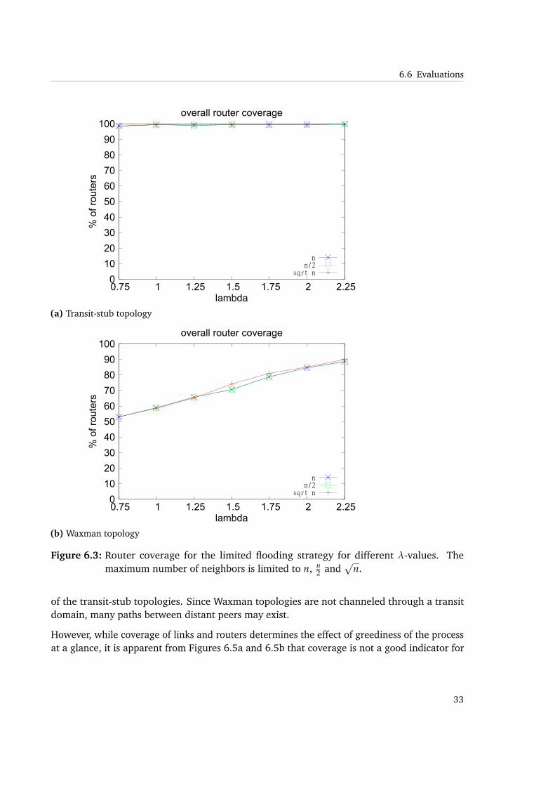
6.2 An exemplary join process of a peer F joining an established discovery overlay. . 266.3 Router coverage for the limited flooding strategy for different λ-values. The
maximum number of neighbors is limited to n, n2 and
√n. . . . . . . . . . . . . 33
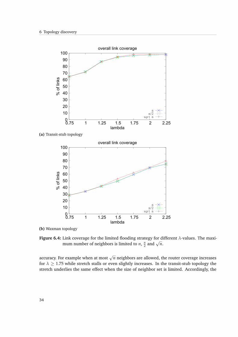
6.4 Link coverage for the limited flooding strategy for different λ-values. Themaximum number of neighbors is limited to n, n
2 and√
n. . . . . . . . . . . . . 346.5 Stretch for the limited flooding strategy for different λ-values. The maximum
number of neighbors is limited to n, n2 and
√n. . . . . . . . . . . . . . . . . . . 35
6.6 Average number of neighbors on the limited flooding strategy for differentλ-values. The maximum number of neighbors is limited to n, n
2 and√
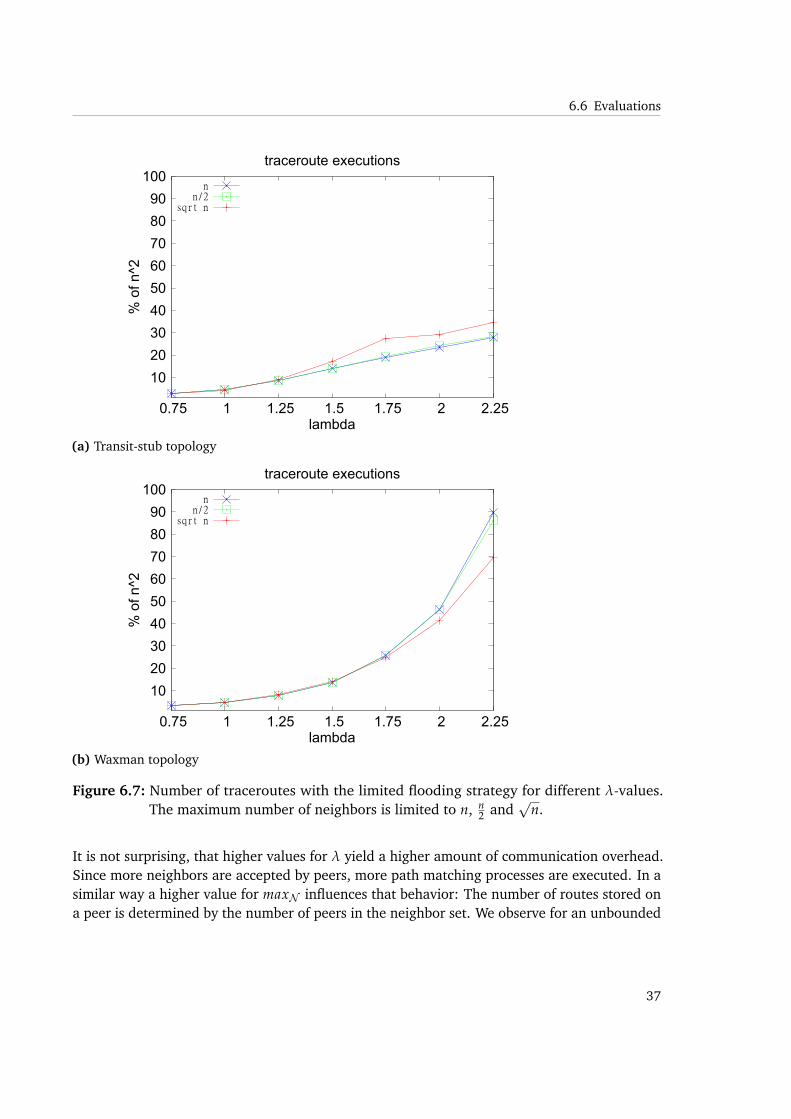
n. . . . . 366.7 Number of traceroutes with the limited flooding strategy for different λ-values.
The maximum number of neighbors is limited to n, n2 and
√n. . . . . . . . . . . 37
6.8 Number of join messages with the limited flooding strategy for different λ-values. The maximum number of neighbors is limited to n, n
2 and√
n. . . . . . 386.9 Link stress ratio with the limited flooding strategy for different λ-values. The
maximum number of neighbors is limited to n, n2 and
√n. . . . . . . . . . . . . 40
6.10 Router coverage for the random walk strategy for different σ-values. . . . . . . 426.11 Link coverage for the random walk strategy for different σ-values. . . . . . . . . 436.12 Stretch for the random walk strategy for different σ-values. . . . . . . . . . . . 446.13 Link stress ratio for the random walk strategy for different σ-values. . . . . . . . 456.14 Average number of neighbors for the random walk strategy for different σ-values. 466.15 Number of traceroutes for the random walk strategy for different σ-values. . . . 476.16 Number of join messages for the random walk strategy for different σ-values. . 48
7.1 A Minimum Spanning tree failing to approximate a Minimum Routing Cost Treeof a given topology. A similar observation was made by Chao et al.[7] . . . . . . 50
7.2 The core of the graph is a tree connecting the relay nodes. . . . . . . . . . . . . 53
5
7.3 Overlay routing stretch compared to discovery overlay for different λ-values.The maximum number of neighbors is limited to n. . . . . . . . . . . . . . . . . 62
7.4 Overlay routing stretch compared to the underlay network for different λ-values.The maximum number of neighbors is limited to n. . . . . . . . . . . . . . . . . 63
7.5 Overlay routing stretch compared to discovery overlay for different λ-values.The maximum number of neighbors is limited to
√n. . . . . . . . . . . . . . . . 65
7.6 Overlay routing stretch compared to the underlay network for different λ-values.The maximum number of neighbors is limited to
√n. . . . . . . . . . . . . . . . 66
List of Tables
6.1 Characteristics of generated router-level topologies . . . . . . . . . . . . . . . . 31
List of Algorithms
7.1 Init Peer (at node u) . . . . . . . . . . . . . . . . . . . . . . . . . . . . . . . . . 567.2 OnReceive(at node u) . . . . . . . . . . . . . . . . . . . . . . . . . . . . . . . . 577.3 CheckSync(at node u) . . . . . . . . . . . . . . . . . . . . . . . . . . . . . . . . 577.4 OnReceive(at node u) . . . . . . . . . . . . . . . . . . . . . . . . . . . . . . . . 587.5 CheckSync(at node u) . . . . . . . . . . . . . . . . . . . . . . . . . . . . . . . . 58
6
1 Abstract
Providing delay-reduced routing is important in publish-subscribe systems where timely de-livery of event notifications is a critical factor affecting system operation or user experience.However, common research focused primarily on alleviating false-positives. More recent ef-forts aim towards quality related issues through adapting the overlay according to subscriberrequirements but leaving underlying network characteristics aside.
It is commonly accepted that efficient routing can only be achieved when underlying networkcharacteristics are respected. Even so, incorporating underlay-aware strategies to build low-stretch overlays is not considered in many distributed environments.
This work focuses on solving the problem of establishing an efficient underlay-aware routingmechanism in a content-based publish-subscribe system. In particular, we strive to reduceend-to-end delay among communication partners. Thereby, our contributions are twofold:We will develop a topology inference scheme for unstructured peer-to-peer networks andintroduce a routing mechanism reducing overall end-to-end delay among peers. Experimentalevaluations will be given for different Internet-like router topologies showing that the approachis capable of modeling an underlay network in an efficient and accurate manner. Furthermore,we will show the positive impact on the stretch of the overlay to outline the concept as a sourcefor efficient event notification delivery in a publish-subscribe environment.
7

2 Introduction
Operation of distributed applications in dynamic environments is influenced by many factors.In general systems, poor performance may only cause impaired user experience, while in moresophisticated systems like stock exchange applications or environmental monitoring systems,providing timely delivery of event notifications is an essential requirement. Du to the tightcoupling of the latter applications to real-world incidents where squandering time may directlyresult in loss of economic wealth or even physical inviolability.
A crucial factor to performance in that context is reducing end-to-end delay between hosts.It is therefore critical to relate overlay connections to network links exhibiting low latency.Necessary information to implement such a behavior is not at hand without prior efforts. Beingable to take network characteristics into account requires inferring of topology informationfirst. Approaches that gain and incorporate such knowledge to a certain degree are said to beunderlay-aware.
The ratio between the end-to-end latency of the overlay and the network-level delay can bemeasured and is commonly referred to as stretch. It has significant impact on routing cost as itdefines the lower bound of the achievable performance.
Dealing with environments where communication partners are dynamically changing anddecoupled adds to the complexity of the problem. The publish-subscribe paradigm is a typicalrepresentative of such environments as message consumers are addressed indirectly by thecontent of a message rather than by name or identifier. Participants may express their interestsin specific events by issuing subscriptions. Events are emitted by publishers without knowledgeof receivers, therefore notifications have to be propagated throughout the network deliberatelyto reach subscribers.
The expressiveness varies in the different types of subscriptions. Topic-based subscriptionsfor instance are limited to predefined subjects, while content-based subscriptions permit thedefinition of attributes and allow filtering on content making them serve a more expressivepurpose.
One can categorize the different architectures providing the upper mentioned capabilities ofpublish-subscribe systems as follows: The common approach implements message brokers.Each participant connects to a broker using a dedicated overlay where event notifications aredisseminated solely among brokers. Most recent research however is focusing on techniquesthat implement peer-to-peer overlays where participants have equal abilities.
9
2 Introduction
In this thesis, we will study the problem of establishing an efficient, underlay-aware routingmechanism for unstructured peer-to-peer environments. The objective is to contribute toquality of service in content-based publish-subscribe systems. We are proposing a distributedtopology inference scheme that maintains a peer-to-peer overlay based upon overlappingpaths on the router-level. Our second contribution will be the development of a mechanismreducing overall routing cost by decreasing end-to-end delay between peers. Therefore, wewill introduce a distributed algorithm building and maintaining an approximate minimumrouting cost spanning tree. The routing overlay is used to establish a content-based publish-subscribe system that uses a filter-based approach to propagate event notifications and toreduce false-positives.
We will show experimentally that the inference scheme is able to draw an accurate low-stretchrepresentation of the underlying network. Simulations reveal that achievable stretch is notexclusively related to inference overhead, but also to the amount of dedicated local space.Values close to the optimum can be reached calling for significantly less communicationoverhead compared to the naive n-by-n approach. Furthermore, simulations show that therouting mechanism is capable of achieving improved results compared to other approaches.
This thesis is structured as follows: After discussing related work in the following chapter, wewill define the system model and formulate the problem statement. An approach overviewis given in chapter 5, while the process of topology discovery and routing are detailed inchapters 6 and 7. The last chapter concludes the work and offers a prospect of possible futurework.
10
3 Related work
In the following, we will briefly introduce related work that aims towards providing quality ofservice in terms of routing cost reduction in publish-subscribe systems and general overlays.
3.1 QoS in publish-subscribe systems
Tariq et al. [25] recently proposed an approach to satisfy subscriber-defined delay require-ments in a publish-subscribe environment: Subscribers maintain the overlay by establishingconnections in a peer-to-peer system. To balance the trade-off among reducing false-positivesand improving scalability. The authors distinguish between two types of subscriptions, namelyuser-level and peer-level subscriptions. User-level subscriptions represent the original interest,while the peer-level subscriptions define the notifications a peer receives due to forwarding.The peer-level subscription is generated by spatial indexing within a decomposed event space.Subscribers satisfy their delay requirements by connecting to peers having tighter requirementsand covering subscriptions. They rely on the conjuncture that those peers in turn will connectto proper peers.
While the authors show that their proposed system is robust and scales well, the givenapproach is not considering underlay characteristics in detail. Since we are focusing onunderlay-awareness, the proposed concepts are not implicitly conferrable.
Majumder et al. [18] developed a routing framework that groups subscriptions based onsimilarity to reduce communication overhead: Each group maintains a dissemination tree withminimized cost. Computing such a tree is a generalization of the Steiner tree problem. Theauthors designed approximation algorithms that use low-stretch spanning trees and prove thatthe cost is within a poly-logarithmic factor of the optimum.
The dissemination tree is built using a centralized approach and deployed in a broker-basedpublish/subscribe environment. Our work is paying special attention on decentralized peer-to-peer systems postulating that every participant is capable of fulfilling all tasks involved.
The approach of Jaeger et al. [12] considers broker overlays and seeks a delivery tree thatspans only brokers that are interested in a specific notification: The authors define the costfor the distribution of a single notification as the sum of processing costs induced by involvedbrokers and the communication cost of using links between them. The overall cost to distribute
11
3 Related work
all notifications shall be minimized which gives the Pub/Sub Overlay Optimization Problem(PSOOP). The authors show that the corresponding decision problem is NP-complete anddevelop a Cost and Interest heuristic that aims to respect cost and reduce the distance betweenbrokers that consume many identical notifications. Therefore, brokers cache their notificationsand compare them to other caches by using Bloom filters. Since brokers only have localknowledge, they run a evaluation and consensus phase before reconfigurations may occur.
While the approach certainly contributes to quality of service, a broker-based approach againserves different prerequisites.
3.2 QoS in overlays
Beyond the scope of publish-subscribe systems more effort is spent on considering networkcharacteristics in overlay construction. The approaches summarized in this section werecontributing to our work by gaining a wider knowledge of established techniques to supportquality of service.
Zhu et al. [34, 33] modeled link correlations as linear constraints and proposed a distributedalgorithm constructing flow-rate optimized overlays through finding hidden bottlenecks. Over-lay links are considered to be correlated if they correspond to paths in the underlay, sharingat least one physical link. The distributed algorithm uses multiple steps. First, it utilizes aprobing tool to detect shared bottlenecks based on inter-arrival times of packets among a groupof hosts. The groups are partitioned to derive linear capacity constraints (LCC) from smallersubgroups while maintaining a global set of constraints. The step of dividing is repeated untilall constraints are found. The authors further study two network flow problems, maximumflow and widest path with the addition of LCC and show that the latter is NP-complete.
In group multicasting every member may multicast to others belonging to the same group. Theproblem of group multicasting routing with delay constraints (DCGMRP) is addressed by Lowet al. [17]: Since the problem is NP-complete, a heuristic algorithm is developed. Each memberof the group maintains its own delay-bounded multicast tree. The algorithm constructs a set ofminimum delay multicast trees using Dijkstra’s algorithm as an initial solution. Then the overallsolution is iteratively improved by finding the busiest link (which is the one with the largestlink usage), locating the multicast trees that contain that link, and adjusting the trees to reducethe usage of that link while at the same time satisfying delay constraints.
Parmer et al. [21] show several multicast tree construction algorithms to meet subscriber-defined QoS constraints. The authors define functions that detect nodes that perform bestand worst in several latency and route related metrics. They propose algorithms that swapthose nodes within the multicast tree to support different subscription policies. They concludethat none of the algorithms can be considered as the best, instead they vary in terms of delaypenalty, link stress and cost.
12
3.3 Topology inference
3.3 Topology inference
Kwon et al. [16] addressed the construction of a multicast overlay by exploiting underlyingrouter information: Overlaps among routes from a single source to other group membersare used to reduce delay and duplicate packets. They define a process of (shortest) pathmatching, where the overlay tree is partially traversed to determine parents that forwardpackets originating at the source to its children. This is done when the group of participantschanges. The goal is to balance the trade-off among delay and bandwidth. The paths havea significant overlap with the paths determined by routing algorithms, and sharing routeprefixes and establishing forwarding lessens the number of identical packet copies sent alongunderlying links.
The nature of this single-source concept is not targeting towards peer-to-peer overlays. But, wewill show that the process of path matching can be extended from trees to general graphs.
A distributed router-level topology inference approach was developed by Jin et al. [13]. Itis based on a previously proposed centralized approach, called Max-Delta: A server collectstraceroute results from a group of hosts. It selects a set of representative paths for the hoststo discover. The goal is to reveal undiscovered topology information while at the same timetracing less routes from each host. In the distributed version each host sends gained tracerouteinformation to all other hosts. Doing that, every host maintains a partially discovered topology.Information is exchanged via an overlay tree that tries to minimize the tree diameter via anode-degree based heuristic. Also, the authors integrate the Doubletree approach which isaimed to reduce measurement redundancies using a modified version of traceroute.
The proposed concept of recommending targets for traceroute executions differs from ourapproach. Even though the paper substantiates our assumption that giving such suggestionsduring the path matching process will reduce message overhead and will scale even for largeenvironments.
3.4 Approximation algorithms for Minimum Routing CostSpanning Trees
Among all possible spanning trees of a graph, the Minimum Routing Cost Spanning Tree showsthe lowest routing cost possible. Finding such a tree is proven to be an NP-hard problem(see the network design problem called shortest total path length spanning tree in [14, 11]).Therefore, heuristics have to be applied.
Important related work in that particular context of this thesis is proposed by Wu et al. [29, 28]:The authors develop several algorithms that achieve different approximation ratios of theoptimal solution. They utilize a special approximation solution based on a structure referred to
13

3 Related work
as general stars. Ratios between 2 and 43 + ε are achieved by seeking specific subtrees called
separators breaking the overall tree in smaller components. Finding good separators yieldslower approximation ratios.
The algorithms are centralized and runtime is increasing rapidly with tighter approximationbounds. This originates from the fact that the main intention of the authors is to prove theexistence of several approximation ratios, rather than claiming to derive efficient approaches.
The same authors develop algorithms for generalized problems called the Optimal Communica-tion Spanning Tree problems in [28]. Additionally, to an undirected and positively-weightedgraph, a requirement is given for every pair of vertices. The cost between two vertices isexpressed by the requirement multiplied by the path length between them; the special casewhere all requirements are set to 1 is the MRCT problem.
Extending our approach by concepts of this paper is proposed in chapter 8.
A recent paper by Campos et al. [6] proposed an MRCT approximation that we will use amongother approaches to compare our achieved stretch. The authors claim to provide a solutionexhibiting the same routing cost as an MRCT in practice. It is a centralized approach whichmodifies Prim’s well-known MST algorithm: Degree of a node and its adjacent nodes is takeninto account additionally to distance information. By composing those factors a spanningpotential is derived which is used to select a parent node in the spanning tree.
However, to the best of my knowledge there has not been published any distributed algorithmthat approximates an MRCT till to the time of the writing of this thesis.
14
4 System model and problem statement
In the following, we will give a formal description of the system model and formulate theproblem statement. An approach overview is given in chapter 5.
4.1 System model
We strive to provide an underlay-aware approach, therefore we will make certain assumptionsabout the properties of the underlying network. While the approach can easily be extended toasymmetric routes, we will assume that paths on the underlay are stable and symmetric. Thisis necessary for the path matching routine in the join process of peers.
While it is not problematic to presume that peers have distinguishable identifiers, we will alsorequire that property for routers. This may not reflect reality properly due to the existence ofanonymous routers, router aliases and routers with multiple interfaces having different networkaddresses. We will detail in chapter 6.6.3 how such undesired behavior can be addressed usingexisting mechanisms.
The underlay network model of routers and peers exhibits a rather natural graph-theoreticformulation. It is given as follows:
Definition 4.1 (Underlay network) We model the underlay network as an undirected, con-nected graph with non-negative edge weights. It is given by N = (RN ∪ PN , EN , ωN). Theset of vertices is a union of the disjoint finite sets of routers RN and peers PN. The setof links between two arbitrary routers and between routers and peers is defined by EN ⊆(PN × RN) ∪ (RN × RN) ∪ (RN × PN). All links are mapped to their corresponding latencyvalue by the weight function ωN : EN → R≥0.
We require that each peer p ∈ PN is connected to a single router rp ∈ RN and that the edge(p, rp) is contained in EN. We will assume that the last mile delay exhibits low latency and thatprocessing time on a peer to forward messages is negligible. The intuition is that forwardingbetween peers should not be distinctly more expensive than a direct connection as long as thesame underlying routes are involved. The process of forwarding is detailed in chapter 6.
15

4 System model and problem statement
Definition 4.2 (Route) A route ρN : PN × PN → P(EN) is a set of edges that con-nect a peer s to another peer t via a shortest path on N. It is given by ρN(s, t) =
{(s, r1), (r1, r2), ..., (rk−1, rk), (rk, t)} if it traverses the routers ri, i ∈ {1, ..., k} using only edgesfrom that set. For s 6= t, ρN(s, t) contains no cycles.
Definition 4.3 (Delay of a route) The function dN : PN × PN → R≥0 returns the end-to-endlatency of a route between two given peers. It is defined as dN(s, t) = ∑e∈ρN(s,t) ωN(e)
Each peer s ∈ PD is able to infer the route to another t ∈ PD via executing traceroute. Theresult is the actual path on the underlay network that a packet uses by traveling from a routerto another. It is given by ρN(s, t). Each peer s may also ping a target peer t and receives dN(s, t)as a result which is given by:
Both functions ρN and dN are used during the topology discovery process. We will now modelthe discovery overlay D which aims towards giving an accurate representation of the underlaynetwork N based on comparing routes and distances between peers. It emerges from peersinferring routes to other peers and seeking overlaps. The process is discussed in detail inchapter 6. We will only state the preliminaries here.
Definition 4.4 (Topology discovery overlay, neighbor sets) The topology discovery overlayis modeled by an undirected, positively weighted and connected graph D = (PD, ED, ωD). The setPD ⊆ PN is a subset of peers of the network model. It holds all peers that have joined the discoveryoverlay.
Each p ∈ PD is aware of a neighbor set Np ⊂ PD that includes all peers to that it maintains adirect connection. The edge set ED is the union of all those connections of all peers. It is defined asED =
⋃p∈PD{(p, q)|q ∈ Np}. The weight function ωD : ED → R≥0 returns the distance on the
underlying network. So for e = (p, q) we set ωD(e) = dN(p, q).
Neighbor sets are common in peer-to-peer overlays and represent in our case the fact that apeer should only have limited knowledge about the whole topology.
Definition 4.5 (Path on the discovery overlay) Let u, v ∈ PD be peers on the discovery overlay.A path on D is given by a set of edges {(u, h1), (h1, h2), ..., (hk, v)} if it uses the peers hi ∈ PD, i ∈{1, ..., k} as intermediate hops from u to v in the given order. For every edge ( f , g) in a pathg ∈ N f holds. We will denote the shortest path from u to v by ρD(u, v).
Definition 4.6 (Distance on the discovery overlay) The distance dD(u, v) is given by the sumof edge weights of the shortest path that connects u, v ∈ PD, so dD(u, v) = ∑e∈ρD(u,v) ωD(e)
16

4.1 System model
It is common in overlay networks, especially in peer-to-peer networks, to have one or moredesignated bootstrapping nodes, sometimes called rendezvous hosts. They provide informationto newly joining nodes concerning the mechanism of opting in. We will not go into detail abouthow such nodes can be identified, but assume that at least one such host exists and that newparticipants are able to contact it.
The routing overlay R is modeled as an acyclic subgraph of D. All peers of D are spanned in Rbut with a reduced set of edges.
Definition 4.7 (Routing overlay) The routing overlay R is an acyclic, connected subgraph of D.We define R = (PD, ER ⊆ ED, ωD).
Definition 4.8 (Path on the routing overlay) Let u, v be peers in PD. Then the path ρR(u, v)is the unique set of edges that connects that peers on the routing overlay R.
The distance of paths on the routing overlay R is given by the sum of weights of links betweenforwarding peers. It is defined as:
Definition 4.9 (Distance on the routing overlay) Let u, v be peers in PD. The distance on therouting overlay R is given by the corresponding edge weights in D, so
dR(u, v) = ∑e∈ρR(u,v)
ωD(e)
The stretch on R compared to N is related to the overall routing cost of R.
Definition 4.10 (Overall routing cost) The overall cost of the routing overlay R is given by
c(R) = ∑u,v∈PD
dR(u, v)
Definition 4.11 (Stretch) Given a network N and a routing overlay R, we define stretch to bethe ratio of the overall routing cost of R over the sum of minimal achievable end-to-end latency onN for all peers in PD.
stretchN(R) =∑u,v∈PD
dR(u, v)∑u,v∈PD
dN(u, v)
We will now define preliminaries for the process of event notification propagation in thecontent-based publish-subscribe system. We define attributes to have a type, a name and adomain.
17
4 System model and problem statement
Definition 4.12 (Attribute) An attribute attr is given by a tuple (typeattr, nameattr, domainattr).
We define notifications to be a set of typed attributes having a specific value for each attribute.
Definition 4.13 (Constraints) A constraint φ is a tuple (typeφ, nameφ, operatorφ, domainφ). Ifan attribute attr matches a constraint φ we denote that by a ≺ φ.
A filter selects notifications by specifying a set of attributes and a set of constraints on theirdomain. A subscriber can express its interest using a filter as subscription. If a filter containsmultiple constraints for the same attribute, then they are interpreted as a conjunction whichmeans that all constraints must be matched.
So, a notification n matches a filter f if for every constraint φ of that filter, there is an attributea in the notification such that a is matched by φ, formally:
n ≺ f ⇔ ∀φ ∈ f : ∃a ∈ n : a ≺ φ
4.2 Problem statement
Our aim is to solve the problem of establishing an efficient underlay-aware routing mechanismin an unstructured peer-to-peer environment. In particular, we strive to reduce end-to-end delay.In the context of content-based publish-subscribe systems that implies having to propagateevent notifications cost-efficiently through a routing overlay exhibiting low-stretch with respectto the underlying network.
Since we will take network characteristics into account explicitly, we have to derive a discoveryoverlay first. Driving objective is an accurate representation of the underlying network. Theoverhead in terms of both local space and communication shall be as small as possible.Furthermore, we need to maintain a routing overlay that exhibits low overall routing cost toachieve a low stretch.
18
5 Approach overview
The following chapter presents an overview of our solution. We will divide the problem andexplain how the resulting sub-problems are conquered separately (see chapter 4.2 for theproblem statement).
routing overlay
topology discovery overlay
underlay network
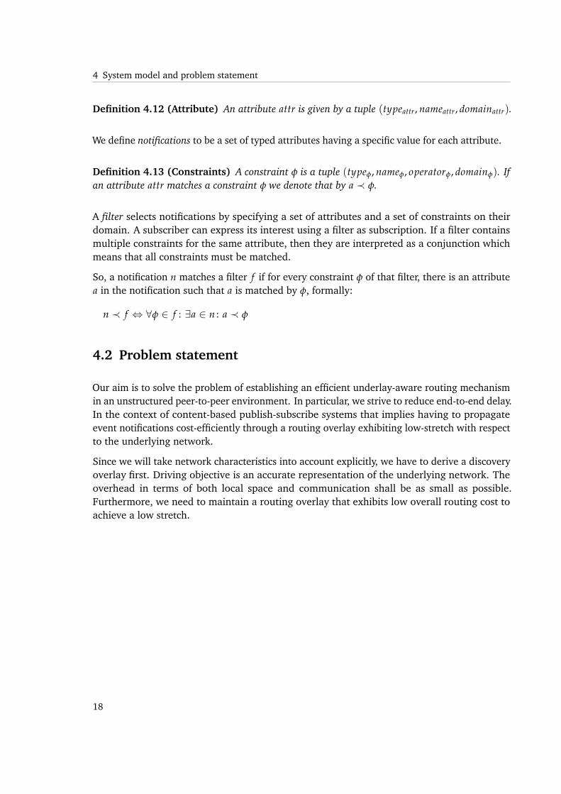
Figure 5.1: Different layers of abstraction having different optimization objectives.
The problem decomposition is depicted in Figure 5.1 and follows along the separation intounderlay network, topology discovery overlay and routing overlay, as stated in the systemmodel. We will first focus on the process of topology inference and discovery overlay con-struction. Subsequently, we will detail the distributed algorithm for the minimum routing costtree approximation forming the routing overlay. Finally, we will explain the adoption of thepublish-subscribe model into this approach.
Topology inference by tracing routes between hosts is costly regarding network operations. Animportant objective of the discovery process is to keep the amount of the operations small.Nevertheless, we have to derive an accurate representation of the underlay network to build ofa low-stretch overlay. Our distributed inferring scheme maintains an unstructured peer-to-peerenvironment. Neighbor sets of peers are rearranged by applying a path matching process basedon router-level information.
19
5 Approach overview
The path matching routine was inspired by the Topology Aware Grouping (TAG) approach byKwon et al.[16]. The authors build an acyclic multicast overlay by applying a process thatexploits overlaps among underlay routes originated from a single source. Following this idea,we will adapt the process to be used in a peer-to-peer overlay. As a result, neighbor sets aremanaged to form a general graph, instead of parent-child relations in a tree. We will permitthe formation of cycles in the discovery overlay to reach a more accurate representation byconsidering routes from all peers.
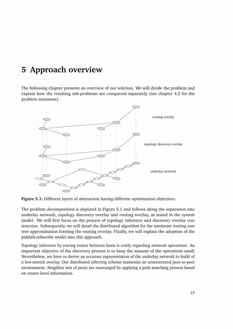
Consider the exemplary situation of a message producer p and the two consumers c1 andc2 in Figure 5.2. The two paths (p, c1) and (p, c2) have a significant overlap of underlyingrouters. If p sends a message to c1 and to c2 subsequently, the overlapping path will be usedtwice. Incorporating the path matching routine, p is able to force a change neighborhood sets.After completion of a rearrangement phase, p can reach c2 by sending a message to c1 that isdelegated to c2. A positive side-effect may arise from link stress reduction. In the decoupledenvironment of publish-subscribe systems, every participant may act as a producer (publisher)as well as a consumer (subscriber).
r1 r2 r3 r4p c2
c1
(a)
r1 r2 r3 r4p c2
c1
(b)
Figure 5.2: Unicast-like message delivery from producer p to consumers c1 and c2 (a) com-pared to underlay-aware message forwarding based on router-level path matching(b). Multiple link usage is depicted by bold lines.
When introducing the routing overlay, the main objective is reducing overall end-to-end delaybetween peers. When considering structures that provide efficient propagation and avoidmultiple delivery, minimum routing cost trees (MRCTs) are the optimal solution, if the distanceon the discovery overlay is used as the cost function.
Since finding such a structure is proven to be an NP-hard problem, we will develop a heuristicthat approximates the MRCT in a distributed manner. We will first derive an alternative way tocalculate the overall routing cost. Subsequently, we show by the resulting formula that thecontribution of an edge to the overall routing cost is not only determined by its weight. Thenumber of times an edge is used on unique shortest paths on the tree highly influences itscontribution. This means in our context that stretch of the routing overlay is influenced byend-to-end delay between peers, and furthermore by the forwarding load of peers.
Our algorithm aims to determine those links having high load forming the future basis of therouting overlay. The first of two phases is called the voting phase, where peers are motivated tovote for their neighbors. Lacking deeper knowledge of the peer-to-peer topology, the choice
20

has to be made solely based on latency information. The peers obtaining the most votes areconsidered to be important for efficient forwarding and therefore incorporated as relay nodes.Furthermore, these peers are connected to each other in order to form a subgraph of therouting overlay that we will call the core. In a second phase, all other peers are connecting tothe core through shortest paths on the discovery overlay.
Considering the publish-subscribe model, we will establish an event routing approach thatbenefits from the shortest path connections in the routing overlay. As a consequence eventnotifications are only propagated in the direction of subscribers having claimed interest before.The routes to be taken are determined by a reverse path mechanism. A reverse path isestablished once a subscription is received, by installing a filter on the receiving peer.
21

6 Topology discovery
In the following, we will describe in detail how the process of network topology inferenceis designed. The overall aim is to build a peer-to-peer overlay that represents an underlyingrouter-level topology in an accurate manner.
We presume the utilization of traceroute-like network diagnostic tools to infer topology charac-teristics. While this enables us to build a precise model of the underlay, the process of gainingthis information is costly. It involves sending multiple ICMP packets with increasing time-to-live to determine intermediate routers on the path to a target host. The routers decrease thetime-to-live of the packet and will respond with an error message once the value reaches zero.The source host is able to construct the list of intermediate routers based on that responses. Anobvious objective for the inference scheme is to avoid as many expensive network operationsas possible.
The driving mechanism of the discovery process is a distributed underlay path matchingroutine.
r1 r2 r3 r4p q
o
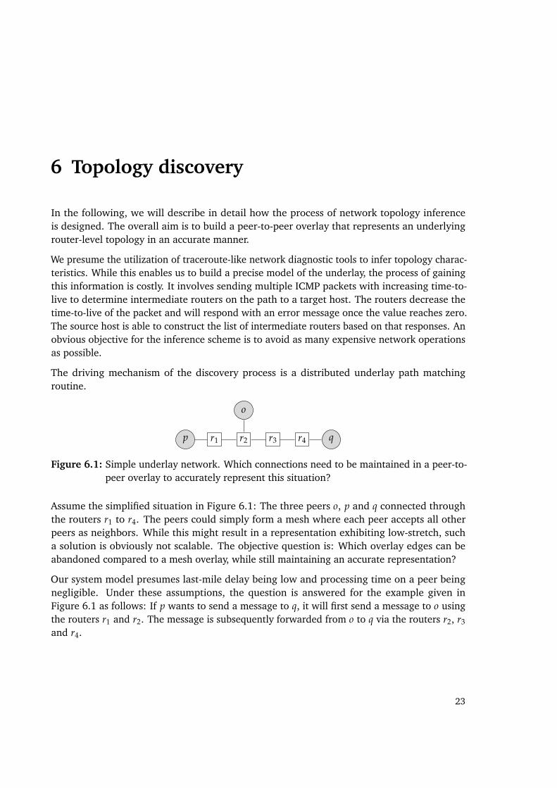
Figure 6.1: Simple underlay network. Which connections need to be maintained in a peer-to-peer overlay to accurately represent this situation?
Assume the simplified situation in Figure 6.1: The three peers o, p and q connected throughthe routers r1 to r4. The peers could simply form a mesh where each peer accepts all otherpeers as neighbors. While this might result in a representation exhibiting low-stretch, sucha solution is obviously not scalable. The objective question is: Which overlay edges can beabandoned compared to a mesh overlay, while still maintaining an accurate representation?
Our system model presumes last-mile delay being low and processing time on a peer beingnegligible. Under these assumptions, the question is answered for the example given inFigure 6.1 as follows: If p wants to send a message to q, it will first send a message to o usingthe routers r1 and r2. The message is subsequently forwarded from o to q via the routers r2, r3
and r4.
23
6 Topology discovery
In a situation where all peers can be consumers and producers of messages at the same time,the neighborhood must be set as follows, to keep the number of overlay edges as low aspossible: Np = {o}, No = {p, q} and Nq = {o}. This guarantees not only a space-efficientrepresentation, but also maintains a low end-to-end delay for all peers.
As a nice side-effect the links stress in the topology discovery overlay is reduced. If for instance,q intends to send the same message to o and p, the forwarding mechanism via o guaranteesthat all links except of o’s connection to its own router are used only once.
Obviously, there is more overhead involved in the management of a peer-to-peer overlay thanmaintaining a set of neighbors, for instance, maintaining socket connections to neighbors. Butin the following chapters, we will allow ourselves a simplification and refer to this problemonly in the context of local space reduction, since the additional overhead is directly related tothe size of the neighbor sets.
In the following, we will give a formal description of the underlay path matching processand the implementation for building and maintaining the discovery overlay. Following that,complexity analysis and evaluations are given below.
6.1 Prefixes
We previously presumed that a peer p stores the resulting route of ρN(p, q) to all its neighborsq ∈ Np. That information enables p to rearrange its neighbor set once it receives a join requestfrom another peer. As mentioned before, the size of the set is a crucial factor to accuracy andspace efficiency of the overall process.
Before the detailed maintenance of the neighbor sets is discussed, we will define the formalfoundation behind the rationale of the process. Therefore, we define prefixes that represent theshared routes.
Definition 6.1 (Prefix) Let p, o, q be peers in PD (p 6= o 6= q). Let ρN(p, o) =
{(p, ro,1), ..., (ro,k, o)} and ρN(p, q) = {(p, rq,1), ..., (rq,k+l , q)} be shortest paths on the networkN (k ≥ 1, l ≥ 0). We call o a prefix of q with respect to p if ro,i = rq,i, ∀i ∈ {1, ..., k}. We willdenote such a situation by o ≺p q.
Consider again the situation in Figure 6.1. In that situation, ρN(p, o) is given by{(p, r1), (r1, r2), (r2, o)}, and ρN(p, q) is {(p, r1), (r1, r2), (r2, r3), (r3, r4), (r4, q)}. Obviously, thepaths overlap on the links from p via the routers r1 and r2. Since additionally, r2 is the routerthat connects o to the network, we say o is a prefix of q with respect to p, denoted by o ≺p q.
Furthermore, if o ≺p q holds, we want to change the neighbor sets such that o forwardsmessages from p to q. Formally expressed we strive to have {(p, o), (o, q)} ⊆ ED, and (p, q) /∈ED. We will now generalize the process to achieve that.
24
6.2 Joining the overlay
6.2 Joining the overlay
Assume the non-trivial case where there are already peers in the discovery overlay (i.e. PD 6= ∅).A peer n (n ∈ PN, but n /∈ PD) wants to opt in, so it contacts a rendezvous node as describedin the system model. We presume that the rendezvous node responds with the name of arandomly chosen peer j ∈ PD. The peer n will now contact j with a join request.
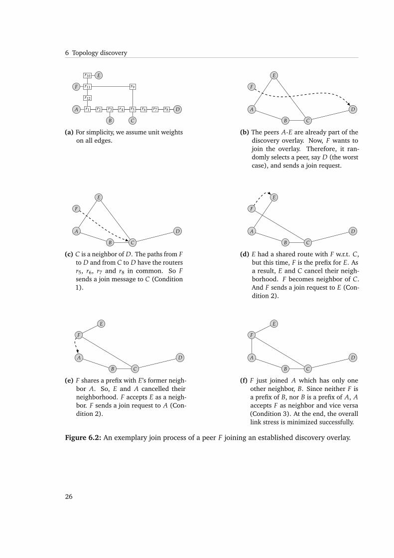
To perform the path matching process, j need to trace the route to n. Knowing the route ton enables j to perform the path matching process and compare the newly discovered routewith routes to its neighbors. There are three mutually exclusive conditions leading to differentactions. For a better understanding, an exemplary join process for a simple unit-weighttopology is given in Figure 6.2.
The first condition handles the case, where j knows a neighbor a that is connected to a routerthat lies on the underlay path from j to the newly joining peer n:
(6.1) : ∃a ∈ Nj : (a ≺j n) ∧ |ρN(j, n)| > |ρN(j, a)|
In that case, n and j will not become neighbors, since they want to benefit from the sharedroute, so j suggests n to join with a instead. Consequently, n will send a join request to a. Anexample for that situation is depicted in Figure 6.2(c).
We will later prove that there is at most one a ∈ Nj that fulfills that condition. In other words,j can’t know any node a′ ∈ Nj (a′ 6= a) that had a shorter prefix of n, having less hops.
If a ≺j n holds, but the second term of the condition does not, the situation is covered by thefollowing condition.
(6.2) : ∃a ∈ Nj : n ≺j a
The peers n and j become neighbors while a and j cancel their current neighborhood relation.The peer n additionally sends a join request to a. Metaphorically speaking, n somehow adoptsa from j.
An example for that situation is depicted in Figure 6.2(d) and 6.2(e).
In the emerging situation, n acts as forwarding peer between j and a. We achieve the desiredresult where (a, j) is removed from ED, while the edge (n, j) is added. The connection betweena and n is established in the separate join process.
If the above conditions did not hold, n and j become neighbors.
(6.3) : neither (6.1) nor (6.2) evaluate to true
25
6 Topology discovery
r10 E
F r11 r9
r12
A r1 r2 r3 r4 r5 r6 r7 r8 D
B C
(a) For simplicity, we assume unit weightson all edges.
E
F
A D
B C
(b) The peers A-E are already part of thediscovery overlay. Now, F wants tojoin the overlay. Therefore, it ran-domly selects a peer, say D (the worstcase), and sends a join request.
E
F
A D
B C
(c) C is a neighbor of D. The paths from Fto D and from C to D have the routersr5, r6, r7 and r8 in common. So Fsends a join message to C (Condition1).
E
F
A D
B C
(d) E had a shared route with F w.r.t. C,but this time, F is the prefix for E. Asa result, E and C cancel their neigh-borhood. F becomes neighbor of C.And F sends a join request to E (Con-dition 2).
E
F
A D
B C
(e) F shares a prefix with E’s former neigh-bor A. So, E and A cancelled theirneighborhood. F accepts E as a neigh-bor. F sends a join request to A (Con-dition 2).
E
F
A D
B C
(f) F just joined A which has only oneother neighbor, B. Since neither F isa prefix of B, nor B is a prefix of A, Aaccepts F as neighbor and vice versa(Condition 3). At the end, the overalllink stress is minimized successfully.
Figure 6.2: An exemplary join process of a peer F joining an established discovery overlay.
26

6.3 Limited flooding strategy
That last condition evaluates to true, if there could not be any path matched on the underlaybetween n and j, or any of j’s neighbors. This is not necessarily an undesired behavior, but mayalso be an indicator that j was not a good choice for n. We will cover that situation later.
The last situation is depicted in Figure 6.2(f).
In the simulations, we will additionally restrict the maximum size of the neighbor sets. In thatcase, a peer will only be added to the neighbor set if it is closer than the currently farthestneighbor in the set which it will replace. If adding n to Nj failed because the maximum size ofthe set is reached and j is not accepted, n is allowed to request a new peer using bootstrappingmechanism.
We will now prove that if there is an a in Nj that is a prefix of n then j cannot know any betterprefix a′ ∈ Nj (a′ 6= a) such that a′ is a possibly shorter prefix of n.
Lemma 6.1 If n joins j and there is an a ∈ Nj : a ≺j n then there cannot be any a′ ∈ Nj : (a′ ≺j
n) ∧ |ρN(j, a′)| < |ρN(j, a)|.
Proof 6.1 Assume, that not only a ∈ Nj but there is also an a′ ∈ Nj : (a′ ≺j n) ∧ |ρN(j, a′)| <|ρN(j, a)|. In that case, a′ would be in the set Nj. Also, a must have joined j to be put in Nj. But,then a path matching between a′ and a would have happened before. During that path matching,condition 6.2 would have evaluated to true, and a would have joined a′ instead, and implies thata /∈ Nj. We reached a contradiction.
We will introduce in the following two strategies designed to cover the situation where no pathmatching was possible on condition 6.3. The strategies are called limited flooding and randomwalk and will be evaluated in combination with the overall join process subsequently.
6.3 Limited flooding strategy
Assume the situation, where a peer n opted in the overlay but unluckily ends up at a positionthat not accurately represents the underlay network condition. As described, this happens ifno successful path matching was possible during the join process.
We propose a strategy covering that situation as follows: Currently, n is connected to a nodej. Since path matching failed, n will now perform a less expensive underlay-aware matchingroutine by starting to measure its distance to peers in the neighborhood of j.
The distance measurement is a valuable indicator whether there are better nearby choices thanj. Even if the neighbors of j did not have overlapping routes, other peers that are multiplehops away on the overlay, may perform better. Since, n doesn’t know these peers, it sends adesignated message to j: That message contains the tuple (n, d, ttl), where d is the underlay
27
6 Topology discovery
distance of n to its nearest neighbor. That message can afterwards be forwarded by j to itsneighbors. Subsequently, the message can be forward again while decreasing the time-to-live.Forwarding is stopped, once a value of 0 is reached.
We introduce the system parameter λ, which we call the locality factor, as it determines thedegree of locality for improvements to n. Peers that receive the previously described tuple areable to guess, whether they would be an improvement for n. They simply evaluate whetherthe following inequality holds:
(6.4) dN(a, n) < λ ∗ d
If that evaluates to true, the peer a knows that it would be an improvement to n, so it acts as ifit would have received a join request from n. Using a higher λ, increases the probability thateven distant peers are sending a join request to n. During that process the path matching isexecuted. So we implemented a lighter version of flooding the neighborhood by using onlydistance measurements, and still get the benefit of possibly overlapping paths of physicallyclose peers after execution of a path matching.
Even if no overlaps exist, once again the condition 6.3 may hold and a and n become neighborsanyway. This is at least an improvement in delay, although paths must not necessarily overlap.The flooding can be regarded as a mechanism that pushes the peer into the right directionbased on distance measurements.
One drawback of that strategy is that the mechanism may still causes many path matchingprocesses. Especially if λ is set to a high value, many peers may consider themselves animprovement for n and will cause traceroute executions. We are able to overcome thatsituation by being more selective when evaluating the inequality 6.4. This can either be doneby a tighter setting for λ, or by limiting the number of neighbors that are flooded. This is thekey factor in the second strategy called random walk.
6.4 Random walk strategy
As described, limited flooding may cause a considerable amount of distance measurements,join messages and traceroute executions in situations, where many hops are necessary onthe overlay. It might cost some hops on the overlay until a peer reaches a decent position,representing the underlay accurately.
The idea behind random walk originates in the assumption, that it might not be necessary toflood the whole neighborhood on every hop. Instead, only a subset of neighbors is selected.Therefore, we introduce the selectivity factor σ representing the chance of each neighborhoodpeer to be chosen for flooding (0 < σ < 1).
28
6.5 Leaving the overlay and node failure
A tight setting for σ lessens the amount of flooding per hop, but raises the probability that a peeris missed, although might have meant an improvement. While discussing the evaluations lateron, we will see that a setting lower as 0.375 performs poorly. Interestingly, taking every secondneighbor into account, performs reasonable, while reducing the amount of join processes andthe number of expensive network operations involved.
6.5 Leaving the overlay and node failure
In the following we will describe, how different situations arising are handled, when a peer pis dropped from the discover overlay through node failure, or intentionally leaves it.
We will consider graceful leave first: Before p disconnects, it can easily determine which of itsneighbors q should send a join message to another neighbor q′. For every situation in whichp ≺q q′ holds, it motivates q to join q′. This restores the underlay-awareness of the overlay.
When p is disconnected caused by node failure, there are two cases that can easily be managed:If a neighbor q ∈ Np is disconnected from the overlay because p fails, it has to rejoin thenetwork by contacting a rendezvous node. If q is not disconnected, it will restore underlay-awareness by running one of the improvement strategies described before.
6.6 Evaluations
We will give a brief complexity analysis of the path matching process and will subsequentlyprovide evaluations.
6.6.1 Complexity analysis
Space complexity is crucial to accuracy of the derived discovery overlay and depends on thesystem parameter maxN : A peer p has to store the routes ρN(p, q) and their length dN(p, q) toits neighbors q ∈ Np. This is necessary to process the underlay path matching process whenreceiving a join request. The number of stored routes is limited by that parameter, so each peerstores at most maxN routes that consist of a number of router identifiers.
It is difficult to give bounds on message complexity, as a join process may lead to other joinprocesses. The number of traceroute executions is proportional to the number of join messages,since at most two of them are executed during that process. We will therefore examine thenumber of join messages and traceroute execution via simulations.
29
6 Topology discovery
6.6.2 Simulations
Experimental setup
In topology generation there exist two major model categories, namely domain-level androuter-level topologies. Both of them are represented as graphs, but with different meaningsof the components: In the domain-level model, nodes depict domains and edges representinter-domain connections, while on the router-level, nodes refer to routers and edges representa one hop connection between them.
Topology generation is an ongoing research topic, so there naturally exist multiple concepts.Caused by the sheer size, lack of persistence and system administrators’ efforts to obscurerouting behavior within a domain, it is very difficult, if not impossible, to verify those models.We can at least try to judge their eligibility. There’s little doubt that the Internet has a significantdegree of hierarchy on both levels: at the router level this is mainly induced by backbonesand at the domain level service providers are broken into tiers [24]. That is one reason, whyAS-level topologies mainly focus on degree distribution (for which a power-law was detected[8, 23]), while imitating hierarchy and locality is the focus of router-level topologies.
For evaluations of our approach, only the latter models are aplicable. To acknowledge diversity,we will generate two models that follow completely different concepts. We aim to determinewhether hierarchy influences the overall accuracy and efficiency of our approach, as well ifdifferent locality affect the quality of the overall process.
We will use BRITE [19] to generate a non-hierarchical Waxman topology [26], and we willutilize GT-ITM [32] to generate a hierarchical transit-stub topology [31] with different domain-roles.
Waxman topologies are commonly used models for generation of random networks. The nodesare placed at random positions in a two-dimensional grid. All possible pairs of nodes areconsidered and the decision whether a link should exist between two nodes is made accordingto a probability function that models locality. One of the parameters, α, increases the generalprobability of edges between any two nodes. The second parameter, β, yields the ratio oflong edges to short edges in the overall topology. The number of links added per node, m,determines the overall number of edges of the topology. We will use the standard settingsα = 0.15 and β = 0.2, but increase the number of links per node (m = 4).
The transit-stub model is used to represent a hierarchical topology. It also places routers in atwo-dimenstional space. One or more transit-domains of routers are inter-connected and anumber of stub-domains is connected to the transit domains. Both domain types are populatedwith a number of routers that are inter-connected based on given probabilities for the domaintype [31, 30]. Our topology contains 4 transit-domains, each consisting of 12 routers and achance of 60% that a link between any two routers exists in a transit domain. The 12 stubdomains are fully linked, each containing 21 routers.
30
6.6 Evaluations
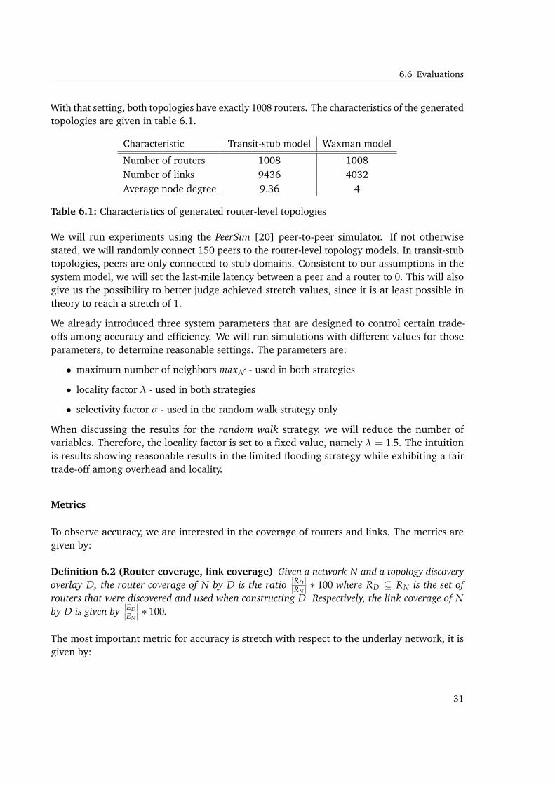
With that setting, both topologies have exactly 1008 routers. The characteristics of the generatedtopologies are given in table 6.1.
Characteristic Transit-stub model Waxman model
Number of routers 1008 1008Number of links 9436 4032Average node degree 9.36 4
Table 6.1: Characteristics of generated router-level topologies
We will run experiments using the PeerSim [20] peer-to-peer simulator. If not otherwisestated, we will randomly connect 150 peers to the router-level topology models. In transit-stubtopologies, peers are only connected to stub domains. Consistent to our assumptions in thesystem model, we will set the last-mile latency between a peer and a router to 0. This will alsogive us the possibility to better judge achieved stretch values, since it is at least possible intheory to reach a stretch of 1.
We already introduced three system parameters that are designed to control certain trade-offs among accuracy and efficiency. We will run simulations with different values for thoseparameters, to determine reasonable settings. The parameters are:
• maximum number of neighbors maxN - used in both strategies
• locality factor λ - used in both strategies
• selectivity factor σ - used in the random walk strategy only
When discussing the results for the random walk strategy, we will reduce the number ofvariables. Therefore, the locality factor is set to a fixed value, namely λ = 1.5. The intuitionis results showing reasonable results in the limited flooding strategy while exhibiting a fairtrade-off among overhead and locality.
Metrics
To observe accuracy, we are interested in the coverage of routers and links. The metrics aregiven by:
Definition 6.2 (Router coverage, link coverage) Given a network N and a topology discoveryoverlay D, the router coverage of N by D is the ratio |RD |
|RN | ∗ 100 where RD ⊆ RN is the set ofrouters that were discovered and used when constructing D. Respectively, the link coverage of Nby D is given by |ED |
|EN | ∗ 100.
The most important metric for accuracy is stretch with respect to the underlay network, it isgiven by:
31
6 Topology discovery
Definition 6.3 (Stretch of the discovery overlay) Given a network N and a topology discoveryoverlay D we define stretch to be the ratio of the shortest path length on D and the network delay
on N between any two peers, which is given by∑u,v∈PD
dD(u,v)∑u,v∈PD
dN(u,v) .
To determine the efficiency of the process, we will also observe the average number ofneighbors that are connected to a peer, as well as the number of join messages that were sentper peer. Furthermore, the overall amount of traceroute executions compared to a naive n-by-napproach.
As described before, we expect reduction in link stress as a side-effect of message forwarding.We define link stress as the number of times an underlay link is used when a peer is sending toa set of targets. To derive sample values for link stress, we assume for the experiments thatpeer identifiers are globally known. Each peer p selects k randomly chosen other peers, wherek ∈ [1, |PD|[. We will plot the ratio of average usage of a link when using unicast-like, butshortest path based routing would be used in N compared to a forwarding mechanism thatuses shortest paths in the overlay D.
Result discussion
As mentioned before, there is a trade-off between the achievable accuracy and the overheadregarding local space and messages. We have introduced the underlay path matching processand two strategies to cover the situation where the matching process fails.
We will first focus on the accuracy of the limited flooding strategy.
Accuracy of limited flooding
It is evident from Figure 6.3(a) that overall router coverage for hierarchical transit-stubtopologies is very high for all values the locality factor λ takes. In the Waxman topology therouter coverage starts low at barely over 50% and needs an increase of λ to grow close to 90%for different settings of maximum allowed neighbors (Figure 6.3(b)).
Nevertheless, the overall router coverage does not seem to be heavily influenced by maxN .That might stem from the fact that the coverage is increasing as new routers are discovered byusing traceroute during the join process, and is not determined by the current values of thedynamically changing neighbor sets. Increasing coverage is an indicator that the choices madeto gain more knowledge are reasonable, asnew routers are discovered.
Link coverage for the Transit-stub topology needs increasing λ to reach values over 90%.Similar to the router coverage, the link coverage for the Waxman topology (figure 6.4b) isimproving with higher λ-values. An explanation for that behavior lies in the building process ofthat type of topology. There is basically a random nature opposed to the hierarchical structure
32
6.6 Evaluations
0
10
20
30
40
50
60
70
80
90
100
0.75 1 1.25 1.5 1.75 2 2.25
% o
f rou
ters
lambda
overall router coverage
nn/2
sqrt n
(a) Transit-stub topology
0
10
20
30
40
50
60
70
80
90
100
0.75 1 1.25 1.5 1.75 2 2.25
% o
f rou
ters
lambda
overall router coverage
nn/2
sqrt n
(b) Waxman topology
Figure 6.3: Router coverage for the limited flooding strategy for different λ-values. Themaximum number of neighbors is limited to n, n
2 and√
n.
of the transit-stub topologies. Since Waxman topologies are not channeled through a transitdomain, many paths between distant peers may exist.
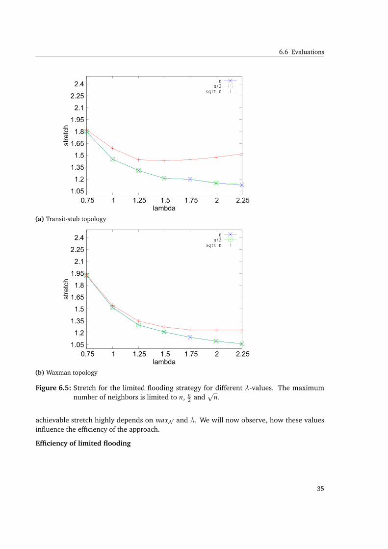
However, while coverage of links and routers determines the effect of greediness of the processat a glance, it is apparent from Figures 6.5a and 6.5b that coverage is not a good indicator for
33
6 Topology discovery
0
10
20
30
40
50
60
70
80
90
100
0.75 1 1.25 1.5 1.75 2 2.25
% o
f lin
ks
lambda
overall link coverage
nn/2
sqrt n
(a) Transit-stub topology
0
10
20
30
40
50
60
70
80
90
100
0.75 1 1.25 1.5 1.75 2 2.25
% o
f lin
ks
lambda
overall link coverage
nn/2
sqrt n
(b) Waxman topology
Figure 6.4: Link coverage for the limited flooding strategy for different λ-values. The maxi-mum number of neighbors is limited to n, n
2 and√
n.
accuracy. For example when at most√
n neighbors are allowed, the router coverage increasesfor λ ≥ 1.75 while stretch stalls or even slightly increases. In the transit-stub topology thestretch underlies the same effect when the size of neighbor set is limited. Accordingly, the
34
6.6 Evaluations
1.05
1.2
1.35
1.5
1.65
1.8
1.95
2.1
2.25
2.4
0.75 1 1.25 1.5 1.75 2 2.25
stre
tch
lambda
nn/2
sqrt n
(a) Transit-stub topology
1.05
1.2
1.35
1.5
1.65
1.8
1.95
2.1
2.25
2.4
0.75 1 1.25 1.5 1.75 2 2.25
stre
tch
lambda
nn/2
sqrt n
(b) Waxman topology
Figure 6.5: Stretch for the limited flooding strategy for different λ-values. The maximumnumber of neighbors is limited to n, n
2 and√
n.
achievable stretch highly depends on maxN and λ. We will now observe, how these valuesinfluence the efficiency of the approach.
Efficiency of limited flooding
35
6 Topology discovery
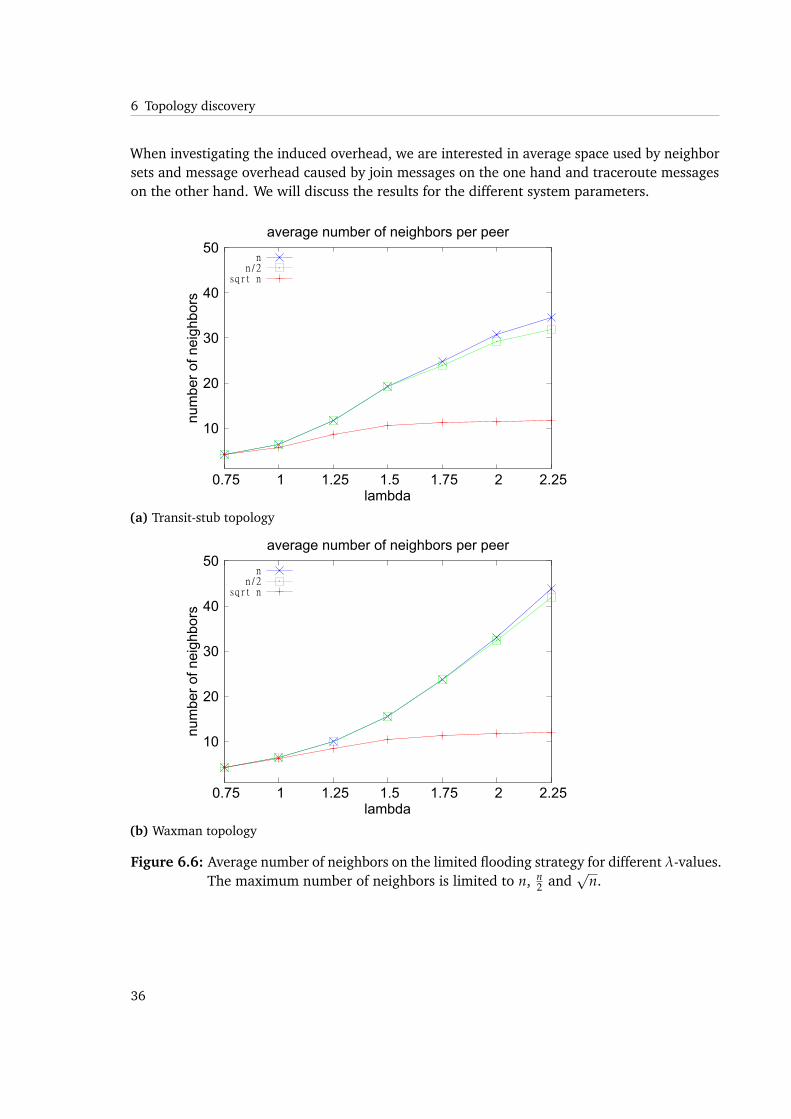
When investigating the induced overhead, we are interested in average space used by neighborsets and message overhead caused by join messages on the one hand and traceroute messageson the other hand. We will discuss the results for the different system parameters.
10
20
30
40
50
0.75 1 1.25 1.5 1.75 2 2.25
num
ber
of n
eigh
bors
lambda
average number of neighbors per peer
nn/2
sqrt n
(a) Transit-stub topology
10
20
30
40
50
0.75 1 1.25 1.5 1.75 2 2.25
num
ber
of n
eigh
bors
lambda
average number of neighbors per peer
nn/2
sqrt n
(b) Waxman topology
Figure 6.6: Average number of neighbors on the limited flooding strategy for different λ-values.The maximum number of neighbors is limited to n, n
2 and√
n.
36
6.6 Evaluations
10
20
30
40
50
60
70
80
90
100
0.75 1 1.25 1.5 1.75 2 2.25
% o
f n^2
lambda
traceroute executions
nn/2
sqrt n
(a) Transit-stub topology
10
20
30
40
50
60
70
80
90
100
0.75 1 1.25 1.5 1.75 2 2.25
% o
f n^2
lambda
traceroute executions
nn/2
sqrt n
(b) Waxman topology
Figure 6.7: Number of traceroutes with the limited flooding strategy for different λ-values.The maximum number of neighbors is limited to n, n
2 and√
n.
It is not surprising, that higher values for λ yield a higher amount of communication overhead.Since more neighbors are accepted by peers, more path matching processes are executed. In asimilar way a higher value for maxN influences that behavior: The number of routes stored ona peer is determined by the number of peers in the neighbor set. We observe for an unbounded
37
6 Topology discovery
10 20 30 40 50 60 70 80 90
100 110 120 130 140 150
0.75 1 1.25 1.5 1.75 2 2.25
num
ber
of m
essa
ges
lambda
join messages per peer
nn/2
sqrt n
(a) Transit-stub topology
10 20 30 40 50 60 70 80 90
100 110 120 130 140 150
0.75 1 1.25 1.5 1.75 2 2.25
num
ber
of m
essa
ges
lambda
join messages per peer
nn/2
sqrt n
(b) Waxman topology
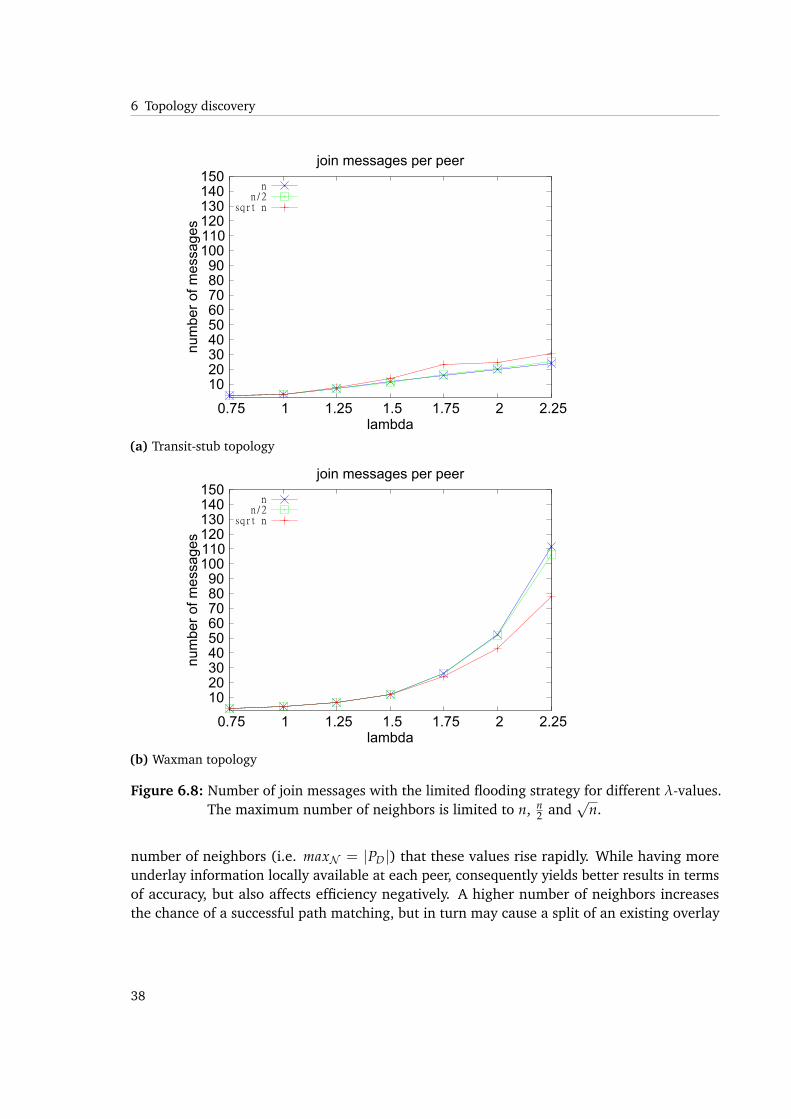
Figure 6.8: Number of join messages with the limited flooding strategy for different λ-values.The maximum number of neighbors is limited to n, n
2 and√
n.
number of neighbors (i.e. maxN = |PD|) that these values rise rapidly. While having moreunderlay information locally available at each peer, consequently yields better results in termsof accuracy, but also affects efficiency negatively. A higher number of neighbors increasesthe chance of a successful path matching, but in turn may cause a split of an existing overlay
38
6.6 Evaluations
connection, resulting in new join messages being issued. As stated before, the number oftraceroute messages is directly related to the number of join messages. The coupling stemsfrom the behavior in path matching, where peers are motivated to to join others (condition 6.1)or are adopting neighbors from other peers (condition 6.2).
We see that in Waxman topologies the amount of join and traceroute messages rises up to 90%for higher values of λ. While transit-stub topologies reach a sort of upper limit as soon as about40% of traceroute messages are executed. As described, the same holds for join messages.While this might be a strange observation on the first sight, we will do another experiment thatwill help to explain that behavior.
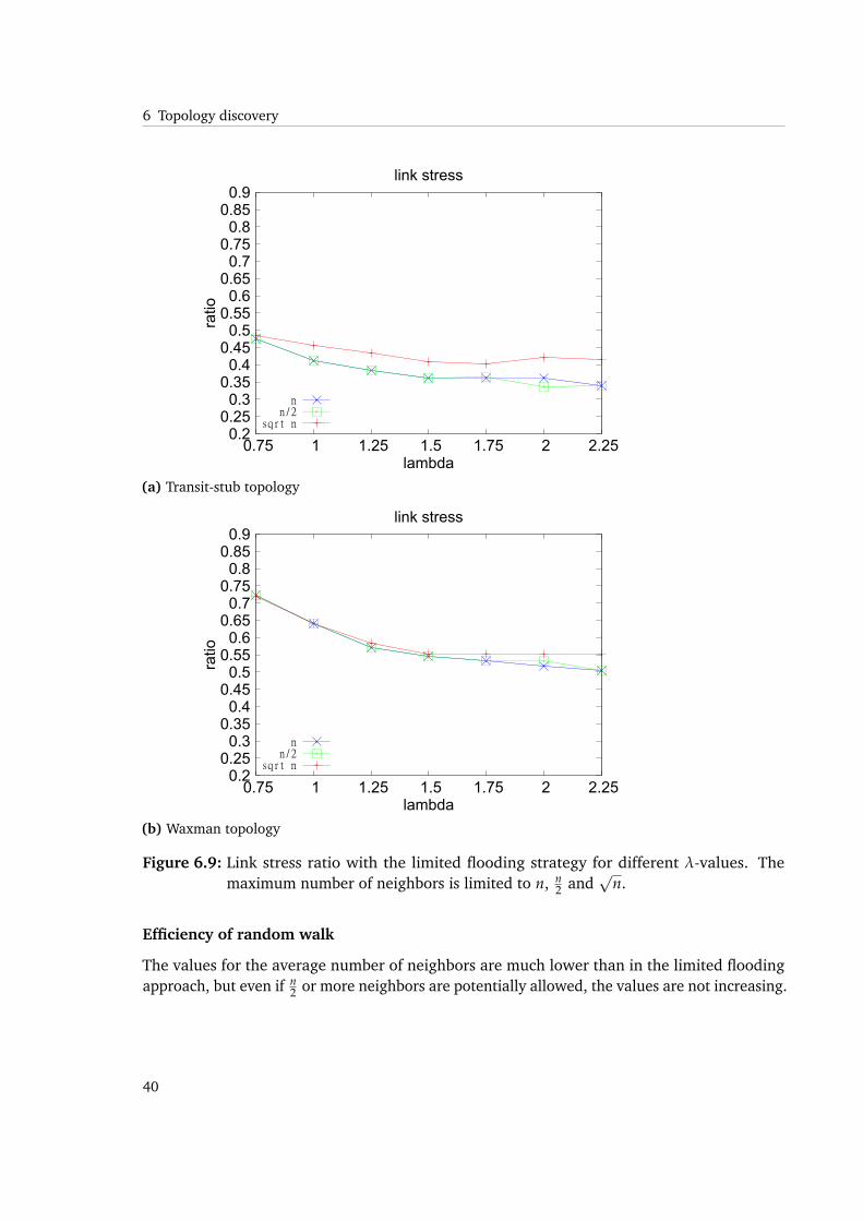
We observe that link stress can be reduced by a factor of 2 to 3 for transit-stub topologies,while in Waxman topologies, it is at least possible to achieve ratios from 0.5 to 0.75 comparedto unicast. This is caused by the same reason, that increases join and traceroute messages. Thedifference in stress reduction derives from messages being channeled through one or moretransit domains. The chance of finding matching prefixes is therefore much higher than inWaxman topologies, where no such separation is enforced, leading to more different pathsbeing available. The path matching process is less likely to find overlapping underlay routes insuch topologies.
Accuracy of random walk
The main focus lies on the different values of σ which determine the amount of probed peers inthe neighborhood. The intention is to randomly choose only a subset of neighboring peers fordistance measurements, which should reduce communication overhead and we will investigateto what extent results are comparable.
We will use the same metrics as in the first strategy and will again examine efficiency of theprocess after having considered accuracy.
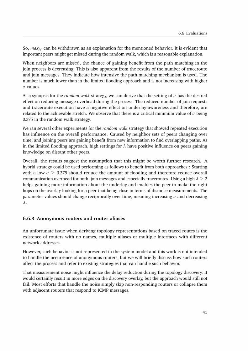
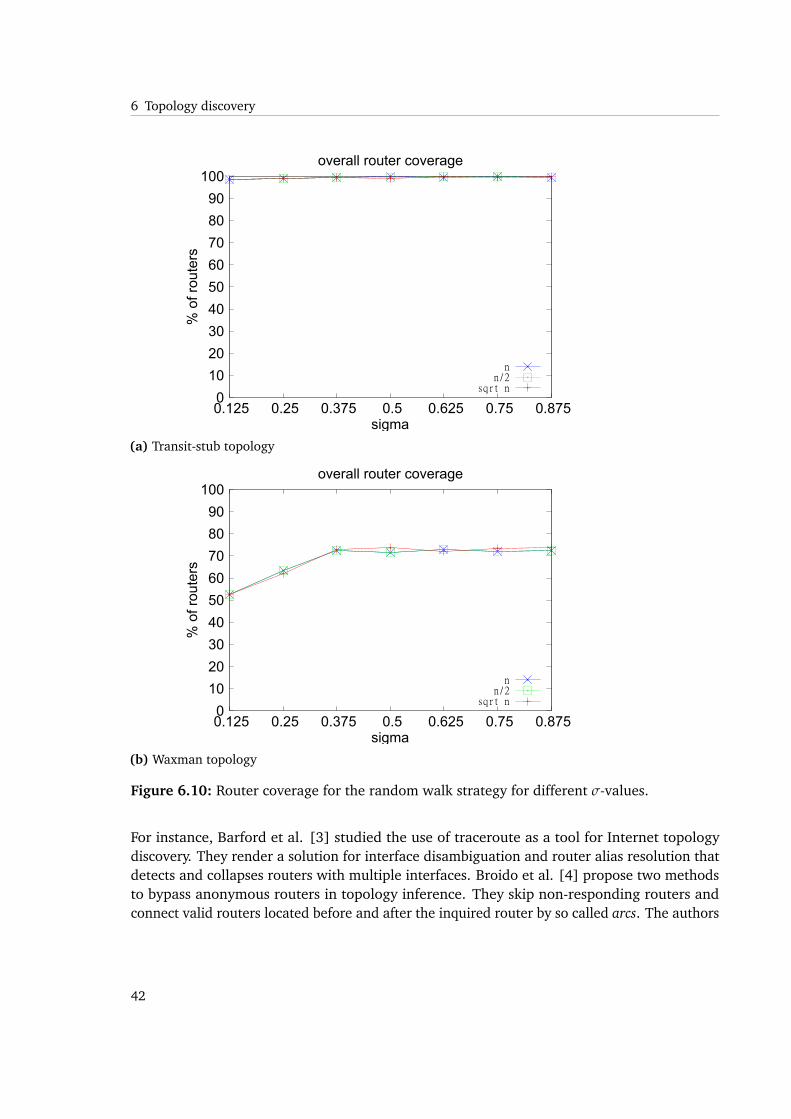
Investigating on less peers also lowers link coverage, while router coverage remains stable. Itis still reasonable for the transit-stub topology that link coverage is increasing with higher σ,reaching similar results as in limited flooding for σ ≥ 0.375. We will determine that this is acritical value.
Keeping in mind that for Waxman topologies, the coverage was highly dependent on thevalue of the locality factor, the random walk results are quite the same for fixed λ, as longas σ ≥ 0.375. High values for λ are necessary to reach 90% router coverage and 80% linkcoverage in limited flooding for Waxman topologies. We also observed that coverage may notbe a good indication for accuracy.
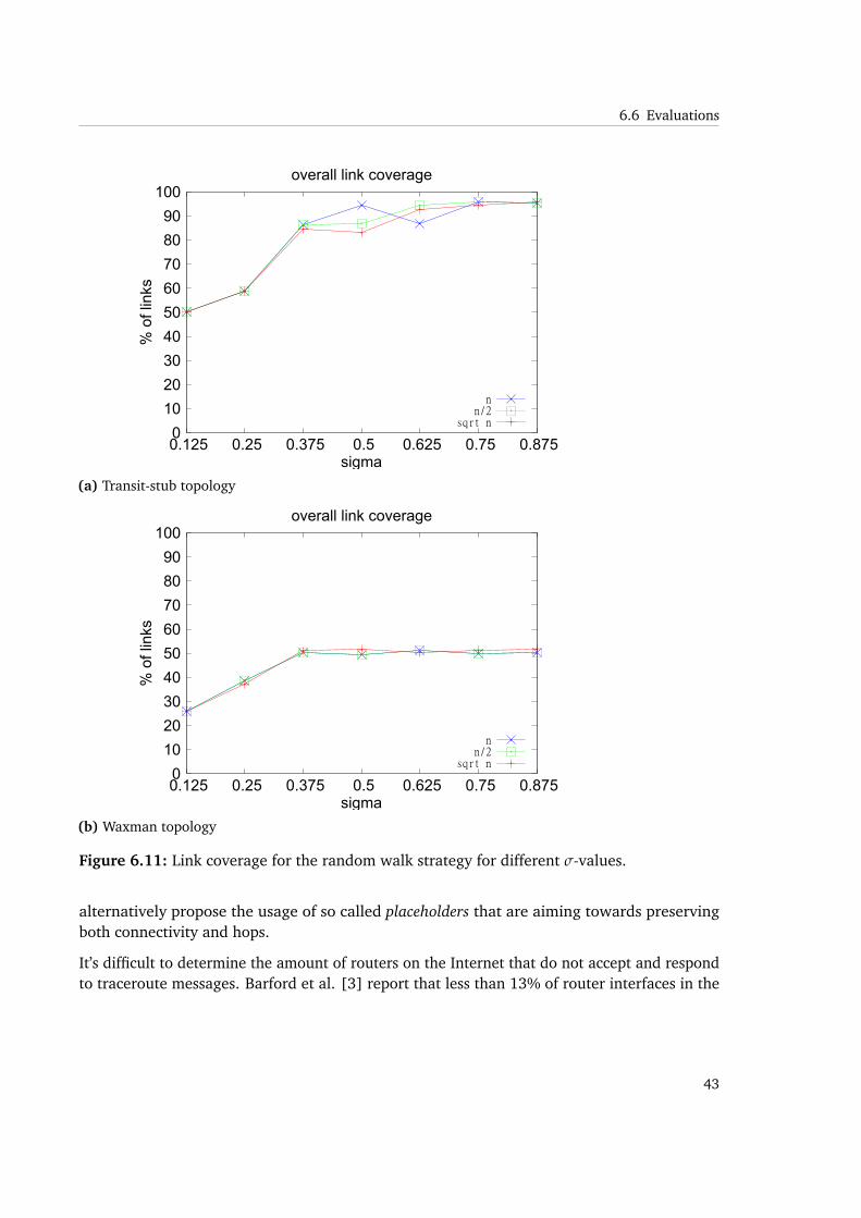
Considering stretch, once again values for σ < 0.375 lead to unreasonable results. We observestretch being bounded even when having σ > 0.5. While not evident from the stretch figure,we can find the reason for this particular behavior while investigating the figure for the averagenumber of neighbors following.
39
6 Topology discovery
0.2 0.25 0.3
0.35 0.4
0.45 0.5
0.55 0.6
0.65 0.7
0.75 0.8
0.85 0.9
0.75 1 1.25 1.5 1.75 2 2.25
ratio
lambda
link stress
nn/2
sqrt n
(a) Transit-stub topology
0.2 0.25 0.3
0.35 0.4
0.45 0.5
0.55 0.6
0.65 0.7
0.75 0.8
0.85 0.9
0.75 1 1.25 1.5 1.75 2 2.25
ratio
lambda
link stress
nn/2
sqrt n
(b) Waxman topology
Figure 6.9: Link stress ratio with the limited flooding strategy for different λ-values. Themaximum number of neighbors is limited to n, n
2 and√
n.
Efficiency of random walk
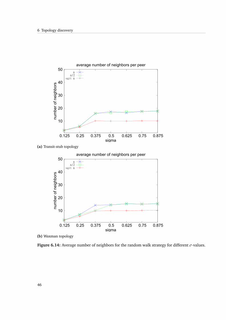
The values for the average number of neighbors are much lower than in the limited floodingapproach, but even if n
2 or more neighbors are potentially allowed, the values are not increasing.
40
6.6 Evaluations
So, maxN can be withdrawn as an explanation for the mentioned behavior. It is evident thatimportant peers might get missed during the random walk, which is a reasonable explanation.
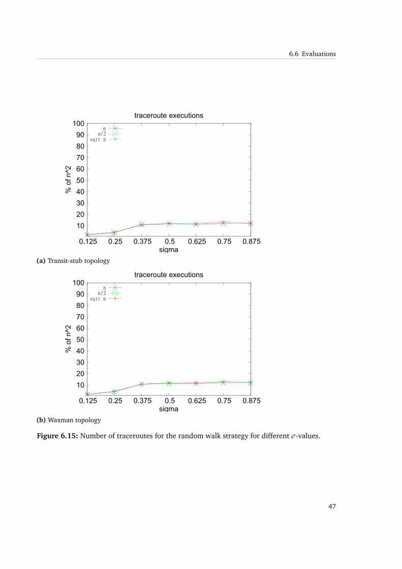
When neighbors are missed, the chance of gaining benefit from the path matching in thejoin process is decreasing. This is also apparent from the results of the number of tracerouteand join messages. They indicate how intensive the path matching mechanism is used. Thenumber is much lower than in the limited flooding approach and is not increasing with higherσ values.
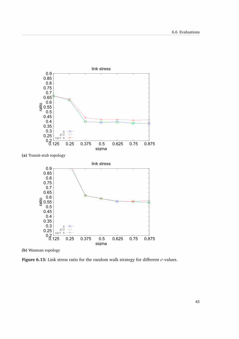
As a synopsis for the random walk strategy, we can derive that the setting of σ has the desiredeffect on reducing message overhead during the process. The reduced number of join requestsand traceroute execution have a negative effect on underlay-awareness and therefore, arerelated to the achievable stretch. We observe that there is a critical minimum value of σ being0.375 in the random walk strategy.
We ran several other experiments for the random walk strategy that showed repeated executionhas influence on the overall performance. Caused by neighbor sets of peers changing overtime, and joining peers are gaining benefit from new information to find overlapping paths. Asin the limited flooding approach, high settings for λ have positive influence on peers gainingknowledge on distant other peers.
Overall, the results suggest the assumption that this might be worth further research. Ahybrid strategy could be used performing as follows to benefit from both approaches:: Startingwith a low σ ≥ 0.375 should reduce the amount of flooding and therefore reduce overallcommunication overhead for both, join messages and especially traceroutes. Using a high λ ≥ 2helps gaining more information about the underlay and enables the peer to make the righthops on the overlay looking for a peer that being close in terms of distance measurements. Theparameter values should change reciprocally over time, meaning increasing σ and decreasingλ.
6.6.3 Anonymous routers and router aliases
An unfortunate issue when deriving topology representations based on traced routes is theexistence of routers with no names, multiple aliases or multiple interfaces with differentnetwork addresses.
However, such behavior is not represented in the system model and this work is not intendedto handle the occurrence of anonymous routers, but we will briefly discuss how such routersaffect the process and refer to existing strategies that can handle such behavior.
That measurement noise might influence the delay reduction during the topology discovery. Itwould certainly result in more edges on the discovery overlay, but the approach would still notfail. Most efforts that handle the noise simply skip non-responding routers or collapse themwith adjacent routers that respond to ICMP messages.
41
6 Topology discovery
0
10
20
30
40
50
60
70
80
90
100
0.125 0.25 0.375 0.5 0.625 0.75 0.875
% o
f rou
ters
sigma
overall router coverage
nn/2
sqrt n
(a) Transit-stub topology
0
10
20
30
40
50
60
70
80
90
100
0.125 0.25 0.375 0.5 0.625 0.75 0.875
% o
f rou
ters
sigma
overall router coverage
nn/2
sqrt n
(b) Waxman topology
Figure 6.10: Router coverage for the random walk strategy for different σ-values.
For instance, Barford et al. [3] studied the use of traceroute as a tool for Internet topologydiscovery. They render a solution for interface disambiguation and router alias resolution thatdetects and collapses routers with multiple interfaces. Broido et al. [4] propose two methodsto bypass anonymous routers in topology inference. They skip non-responding routers andconnect valid routers located before and after the inquired router by so called arcs. The authors
42
6.6 Evaluations
0
10
20
30
40
50
60
70
80
90
100
0.125 0.25 0.375 0.5 0.625 0.75 0.875
% o
f lin
ks
sigma
overall link coverage
nn/2
sqrt n
(a) Transit-stub topology
0
10
20
30
40
50
60
70
80
90
100
0.125 0.25 0.375 0.5 0.625 0.75 0.875
% o
f lin
ks
sigma
overall link coverage
nn/2
sqrt n
(b) Waxman topology
Figure 6.11: Link coverage for the random walk strategy for different σ-values.
alternatively propose the usage of so called placeholders that are aiming towards preservingboth connectivity and hops.
It’s difficult to determine the amount of routers on the Internet that do not accept and respondto traceroute messages. Barford et al. [3] report that less than 13% of router interfaces in the
43
6 Topology discovery
1.05
1.2
1.35
1.5
1.65
1.8
1.95
2.1
2.25
2.4
0.125 0.25 0.375 0.5 0.625 0.75 0.875
stre
tch
sigma
nn/2
sqrt n
(a) Transit-stub topology
1.05
1.2
1.35
1.5
1.65
1.8
1.95
2.1
2.25
2.4
0.125 0.25 0.375 0.5 0.625 0.75 0.875
stre
tch
sigma
nn/2
sqrt n
(b) Waxman topology
Figure 6.12: Stretch for the random walk strategy for different σ-values.
Internet did not respond to traceroute ICMP messages [3]. Broido et al. observe that less than33% of the probed paths in their study contained anonymous or invalid routers.
44
6.6 Evaluations
0.2 0.25 0.3
0.35 0.4
0.45 0.5
0.55 0.6
0.65 0.7
0.75 0.8
0.85 0.9
0.125 0.25 0.375 0.5 0.625 0.75 0.875
ratio
sigma
link stress
nn/2
sqrt n
(a) Transit-stub topology
0.2 0.25 0.3
0.35 0.4
0.45 0.5
0.55 0.6
0.65 0.7
0.75 0.8
0.85 0.9
0.125 0.25 0.375 0.5 0.625 0.75 0.875
ratio
sigma
link stress
nn/2
sqrt n
(b) Waxman topology
Figure 6.13: Link stress ratio for the random walk strategy for different σ-values.
45
6 Topology discovery
10
20
30
40
50
0.125 0.25 0.375 0.5 0.625 0.75 0.875
num
ber
of n
eigh
bors
sigma
average number of neighbors per peer
nn/2
sqrt n
(a) Transit-stub topology
10
20
30
40
50
0.125 0.25 0.375 0.5 0.625 0.75 0.875
num
ber
of n
eigh
bors
sigma
average number of neighbors per peer
nn/2
sqrt n
(b) Waxman topology
Figure 6.14: Average number of neighbors for the random walk strategy for different σ-values.
46
6.6 Evaluations
10
20
30
40
50
60
70
80
90
100
0.125 0.25 0.375 0.5 0.625 0.75 0.875
% o
f n^2
sigma
traceroute executions
nn/2
sqrt n
(a) Transit-stub topology
10
20
30
40
50
60
70
80
90
100
0.125 0.25 0.375 0.5 0.625 0.75 0.875
% o
f n^2
sigma
traceroute executions
nn/2
sqrt n
(b) Waxman topology
Figure 6.15: Number of traceroutes for the random walk strategy for different σ-values.
47
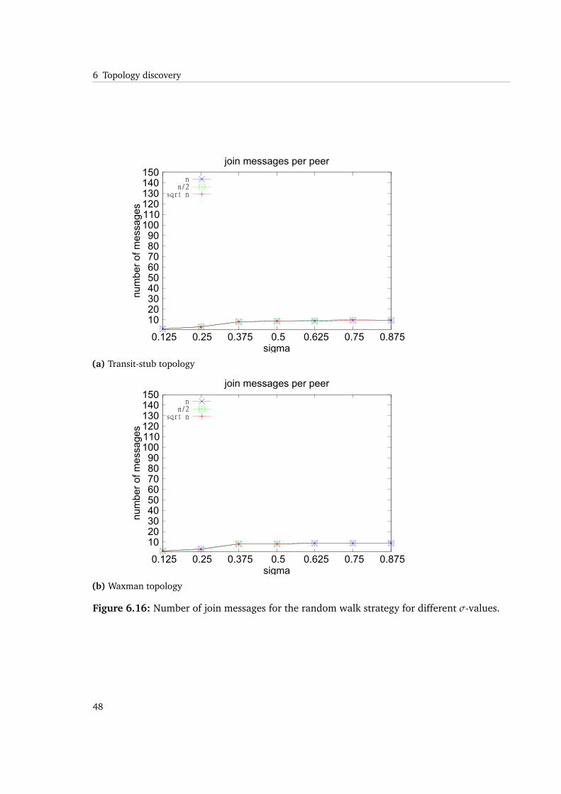
6 Topology discovery
10 20 30 40 50 60 70 80 90
100 110 120 130 140 150
0.125 0.25 0.375 0.5 0.625 0.75 0.875
num
ber
of m
essa
ges
sigma
join messages per peer
nn/2
sqrt n
(a) Transit-stub topology
10 20 30 40 50 60 70 80 90
100 110 120 130 140 150
0.125 0.25 0.375 0.5 0.625 0.75 0.875
num
ber
of m
essa
ges
sigma
join messages per peer
nn/2
sqrt n
(b) Waxman topology
Figure 6.16: Number of join messages for the random walk strategy for different σ-values.
48
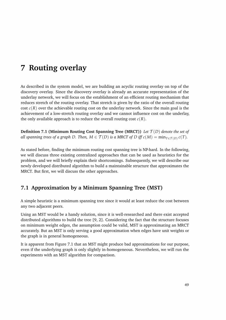
7 Routing overlay
As described in the system model, we are building an acyclic routing overlay on top of thediscovery overlay. Since the discovery overlay is already an accurate representation of theunderlay network, we will focus on the establishment of an efficient routing mechanism thatreduces stretch of the routing overlay. That stretch is given by the ratio of the overall routingcost c(R) over the achievable routing cost on the underlay network. Since the main goal is theachievement of a low-stretch routing overlay and we cannot influence cost on the underlay,the only available approach is to reduce the overall routing cost c(R).
Definition 7.1 (Minimum Routing Cost Spanning Tree (MRCT)) Let T (D) denote the set ofall spanning trees of a graph D. Then, M ∈ T (D) is a MRCT of D iff c(M) = minT∈T (D) c(T).
As stated before, finding the minimum routing cost spanning tree is NP-hard. In the following,we will discuss three existing centralized approaches that can be used as heuristics for theproblem, and we will briefly explain their shortcomings. Subsequently, we will describe ournewly developed distributed algorithm to build a maintainable structure that approximates theMRCT. But first, we will discuss the other approaches.
7.1 Approximation by a Minimum Spanning Tree (MST)
A simple heuristic is a minimum spanning tree since it would at least reduce the cost betweenany two adjacent peers.
Using an MST would be a handy solution, since it is well-researched and there exist accepteddistributed algorithms to build the tree [9, 2]. Considering the fact that the structure focuseson minimum weight edges, the assumption could be valid, MST is approximating an MRCTaccurately. But an MST is only serving a good approximation when edges have unit weights orthe graph is in general homogeneous.
It is apparent from Figure 7.1 that an MST might produce bad approximations for our purpose,even if the underlying graph is only slightly in-homogeneous. Nevertheless, we will run theexperiments with an MST algorithm for comparison.
49
7 Routing overlay
ω
ω
ω
ω
ω
ω
ω
ω
ω− ε
ω− ε ω− ε
ω− ε
ω− ε
ω− εω− ε
ω− ε
(a) Topology. Weights aregiven by ω > ε > 0.
ω
ω− ε
ω− ε ω− ε
ω− ε
ω− ε
ω− εω− ε
(b) Minimum SpanningTree (others possible).
ω
ω
ω
ω
ω
ω
ω
ω
(c) Minimum Routing CostTree.
Figure 7.1: A Minimum Spanning tree failing to approximate a Minimum Routing Cost Tree ofa given topology. A similar observation was made by Chao et al.[7]
7.2 Approximation by a Shortest Path Tree (SPT) rooted at themedian
A shortest path tree rooted at the median of a graph was proposed by Wong et al. [27] as anapproximation for the shortest total path length spanning tree problem [11]. It is possible toachieve a 2-approximation of the MRCT using that approach [28].
Obviously, this structure is highly fragile. When churn occurs, even slight change may cause adifferent node being the median of the graph and will lead to a different tree. That causes theshortest path tree having to be recalculated to keep approximation bounds valid.
Another reason making this structure unfeasible for our purpose, is that median informationis based on summing up all distances from every node to all other nodes. This involvesshortest-path knowledge for all pairs. Determining such global information is inefficient bothin terms of space and messages exchange.
7.3 Approximation by Campos’ algorithm
Campos et al. [6] proposed a fast and simple centralized MRCT approximation. The authorsclaim to be able to provide a solution having the same routing cost as an MRCT in practice.The approach modifies Prim’s minimum spanning tree algorithm: Instead of taking solely edgeweights into account, the algorithm calculates a spanning potential to select a parent node. Itcombines degree of a node, incident edge weights and information about adjacent nodes.
We will include that centralized algorithm in our evaluations.
50
7.4 Approximation by our core-based approach
7.4 Approximation by our core-based approach
Due to unstable results, a distributed minimum spanning tree algorithm is unsuitable, especiallyin heterogeneous topologies.
Developing a distributed algorithm for Campos’ approach is thinkable as it primarily basedon concept of minimum spanning trees. . Even if Campos’ algorithm overcomes some of thedrawbacks of MSTs, the authors admit that it is not possible to derive any propositions aboutthe quality of the outcome [6].
As stated, a problem of using median-rooted SPT is that the properties of the tree dependon a single node that is derived by global knowledge. Small changes in the topology mightinfluence the overall structure. There are some distributed algorithms available, detecting themedian of a graph by comparing all possible SPTs, lacking the possibility of future scaling (see[15, 22]).
Therefore, we will focus to find a more sophisticated structure within the discovery overlayto derive the router overlay: An optimized subgraph of the discovery overlay is constructed,that will be called the core of the graph. The core will consist of nodes that are important foroverall routing cost improvement. It is composed of the high-routing load peers and aims toimprove distant paths between peers. Consequently, we will connect the remaining peers tothe core by using shortest paths on the discovery overlay.
The core is meant to serve a similar purpose on the peer-level as transit-domains do on therouter level. An important difference is allowing the core to change dynamically over time.The core is therefore elected by other peers.Choosing the right edges ER ⊆ ED is the criticalfactor. We will detail that requirements in the following section by analyzing the structure ofminimum routing cost trees and looking for efficient ways to build the routing overlay.
7.4.1 Structure of an MRCT
As a first step, we will analyze the general structure of minimum routing cost trees to explainthe intuition of our solution: The original formula for the routing cost c(R) sums up thedistances between each pair of vertices on the routing overlay. As we cannot derive structuralinformation from the edge weights, we have to observe how often an edge weight is actuallysummed up. The formula counts the usage of each edge e ∈ ρR(u, v) for all u, v ∈ PD. Onmultiplying the usage by the weight of e, we get e’s contribution to overall routing cost.
Lemma 7.1 An edge e ∈ ER that connects the two subtrees induced by the vertex sets V ′ ⊂ VR
and V ′′ ⊂ VR that result by removing e from R is used 2|V ′||V ′′| times.
51

7 Routing overlay
This is evident, if we regard the number of vertices in every emerged subtree. Consider the setof vertices V ′. Every vertex u ∈ V ′ uses e on a path to every v ∈ V ′′. That holds as well for theopposite direction.
Proof 7.1 As in [28]:
∑u∈PD
|{v ∈ PD|e ∈ ρR(u, v)}| = ∑u∈V′|V ′′|+ ∑
u∈V′′|V ′| = 2|V ′||V ′′|
We will call that usage of an edge the load of it. Using the above observation, we can definethe load of an edge by:
Definition 7.2 (Load) The load of an edge e in a tree R that connects the two subgraphs S′ andS′′ that result by removing e is given by
ldR(e) = 2|VS′ ||VS′′ |
Multiplying the load of an edge by its weight permits to calculate the overall routing cost ofthe tree. It leads to the following lemma:
Lemma 7.2 An alternative formula of the overall routing cost c(R) of a tree R is given by
c(R) = ∑e∈ER
ldR(e)ωR(e)
Proof 7.2 As in [28]: Let ρR(u, v) denote the path from a node u to a node v on the tree R. Then,
c(R) = ∑u∈PD
(∑
v∈PD\{u}dR(u, v)
)
= ∑u∈PD
∑v∈PD\{u}
∑e∈ρR(u,v)
ωR(e)
= ∑
e∈ER
(∑
u∈PD
|{v ∈ PD|e ∈ ρR(u, v)}|)
ωR(e)
= ∑e∈ER
ldR(e)ωR(e)
While not solving the actual problem, we can at least observe that there are certain edges thatmight contribute more to the overall routing cost than others. Edges with a high routing loadcontribute multiple times with their weight. Therefore, finding edges exhibiting both highrouting load and low weight, will overall yield a low routing cost.
52
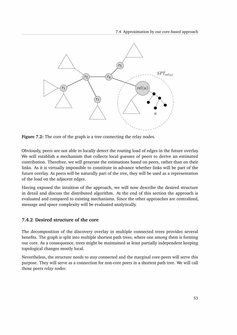
7.4 Approximation by our core-based approach
r1
r2
r3
r4
r5
rel(u)
SPTrel(u)
u
Figure 7.2: The core of the graph is a tree connecting the relay nodes.
Obviously, peers are not able to locally detect the routing load of edges in the future overlay.We will establish a mechanism that collects local guesses of peers to derive an estimatedcontribution. Therefore, we will generate the estimations based on peers, rather than on theirlinks. As it is virtually impossible to constitute in advance whether links will be part of thefuture overlay. As peers will be naturally part of the tree, they will be used as a representationof the load on the adjacent edges.
Having exposed the intuition of the approach, we will now describe the desired structurein detail and discuss the distributed algorithm. At the end of this section the approach isevaluated and compared to existing mechanisms. Since the other approaches are centralized,message and space complexity will be evaluated analytically.
7.4.2 Desired structure of the core
The decomposition of the discovery overlay in multiple connected trees provides severalbenefits. The graph is split into multiple shortest path trees, where one among them is formingour core. As a consequence, trees might be maintained at least partially independent keepingtopological changes mostly local.
Nevertheless, the structure needs to stay connected and the marginal core-peers will serve thispurpose. They will serve as a connection for non-core peers in a shortest path tree. We will callthose peers relay nodes:
53
7 Routing overlay
Definition 7.3 (Core, Relay node) We will denote the set of peers in the core by C. We call anode rel(u) ∈ C the relay node of u if it has the minimum distance to u among all nodes in C. So,dR(u, rel(u)) = minr∈CdR(u, r). The shortest path tree rooted at rel(u) is denoted by SPTrel(u).
Paths on the routing overlay in general start at a peer u in a branch of the tree SPTrel(u), usinga shortest path to the relay node rel(u) ∈ C, allowing them to reach other overlay peers, asdepicted in Figure 7.2.
Using that structure, enables us to give an upper bound on the path distance in R:
dR(u, v) ≤ dSPTrel(u)(u, rel(u)) + dC(rel(u), rel(v)) + dSPTrel(v)
(rel(v), v)
More detailed bounds are discussed in chapter 7.8. But firstly, we will focus on the algorithmin the following section.
7.5 Distributed algorithm
Our approach forms the routing overlay by connecting multiple shortest path trees. Solvingshortest path related problems is a sub-problem of many routing protocols or network opti-mization algorithms in general. It often turns out to be the performance bottleneck of themas well. Depending on the algorithm used, it has negative influence on either time, space ormessage complexity.
Most of the algorithms have in common to use the basic formulation of the Bellman inequality.It is a rather local property that expands globally. It describes the optimal substructure propertyof shortest paths stating that any shortest paths is composed of further shortest paths [28]. Wewill take advantage of that property in the following.
Peers are influenced by that local property to optimize routes by determining shortest paths intheir neighborhood. We may assume that nodes connected to edges causing an improvementare important.
The main algorithm consists of two separate phases: The voting phase and the connectionphase.
7.5.1 Voting phase
The peers form a spanning tree for temporary communication. Any distributed spanning treealgorithm is sufficient, for instance as proposed by Awerbuch [2]. The peers will attempt toinfluence the formation of the core to their advantage. Each peer elects among its neighboringpeers while all votes are gathered by sending them along the spanning tree. Peers receiving
54
7.5 Distributed algorithm
higher votes are considered to be important due to their low-latency link. Peers that acquiredmore than the average amount of votes will form the core after being informed by the root ofthe temporary spanning tree. Each relay node r ∈ C is aware of being part of the core.
In detail, the algorithm is implemented similar to the synchronizer β by Awerbuch [1]: In aninitialization phase a spanning tree is formed and the root is a temporary leader in the network.The leader sends a message along the tree, notifying other nodes that the voting process maycommence. Starting at the leaves of the temporary spanning tree, the votes are summed upand propagated towards the leader. The temporary root can now distinguish non-core peersfrom the relay nodes by summing up the votes each peer has received from other peers. Thetemporary structure is then used to inform all peers about the relay nodes.
7.5.2 Connection phase
The remaining non-core peers have to choose one of the relay nodes from the core as it is notguaranteed that one of the peers they voted for eventually made it to the core. The challengeis that peers have to choose the closest of the core even if it is multiple hops away and they arenot aware of the distance.
A peer u has to find the closest relay node rel(u) ∈ C and take a position in the shortest pathtree SPTrel(u) rooted at that relay node. Therefore, each peer executes the Init Peer procedureproposed in Algorithm 7.1: In this state, no routing information to the core is known. If a peerdetects that itself as being part of the core, it will immediately inform its neighbors. Non-corepeers need to send a 〈sync〉-message. After the initialization exactly 2 messages have been sentalong each link.
The peers keep track of an estimated distance to the relay nodes. They might receive messagesfrom neighbors containing the neighbor’s distance estimate to a relay node. A peer recomputesthe value by adding the distance to the neighbor and might set the neighbor as the next hop tothe relay node, in case of providing an improvement.
Each distance update would potentially cause a flood of updates to other nodes. We strive toavoid such a distance update causing a complete change on all connected descendants in theshortest path tree. Therefore, our algorithm uses a synchronization approach as introduced byAwerbuch et al. [1], reducing the amount of messages produced. Peers consider a phase to befinished once they have received a message from all of their active neighbors.
55
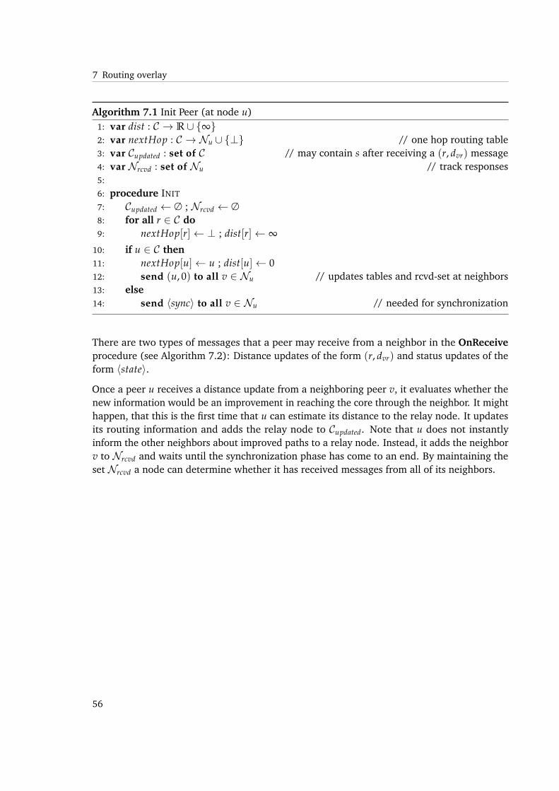
7 Routing overlay
Algorithm 7.1 Init Peer (at node u)1: var dist : C → R∪ {∞}2: var nextHop : C → Nu ∪ {⊥} // one hop routing table3: var Cupdated : set of C // may contain s after receiving a (r, dvr) message4: var Nrcvd : set of Nu // track responses5:
6: procedure INIT
7: Cupdated ← ∅ ; Nrcvd ← ∅8: for all r ∈ C do9: nextHop[r]← ⊥ ; dist[r]← ∞
10: if u ∈ C then11: nextHop[u]← u ; dist[u]← 012: send (u, 0) to all v ∈ Nu // updates tables and rcvd-set at neighbors13: else14: send 〈sync〉 to all v ∈ Nu // needed for synchronization
There are two types of messages that a peer may receive from a neighbor in the OnReceiveprocedure (see Algorithm 7.2): Distance updates of the form (r, dvr) and status updates of theform 〈state〉.
Once a peer u receives a distance update from a neighboring peer v, it evaluates whether thenew information would be an improvement in reaching the core through the neighbor. It mighthappen, that this is the first time that u can estimate its distance to the relay node. It updatesits routing information and adds the relay node to Cupdated. Note that u does not instantlyinform the other neighbors about improved paths to a relay node. Instead, it adds the neighborv to Nrcvd and waits until the synchronization phase has come to an end. By maintaining theset Nrcvd a node can determine whether it has received messages from all of its neighbors.
56

7.5 Distributed algorithm
Algorithm 7.2 OnReceive(at node u)1: procedure ONRECEIVE(r, dvr) // dvr is v’s current distance estimate to a relay node r ∈ C2: if (u /∈ C) ∧ (dist[r] > ω(u, v) + dvr) then // would (u, v) help to better reach r?3: nextHop[r]← v // update routing table4: dist[r]← ω(u, v) + dvr
5: Cupdated ← Cupdated ∪ {r} // because dist[r] was improved
6: Nrcvd ← Nrcvd ∪ {v} // We will not send the improvement right now...7: CheckSync() // ...but wait until received from all (’sync’)
8:
9: procedure ONRECEIVE(state) // sent by neighbor v10: if state = 〈sync〉 then11: Nrcvd ← Nrcvd ∪ {v}12: CheckSync()
Once having received a message from a neighbor, a peer runs CheckSync (see Algorithm 7.3).It evaluates, whether it has reached the end of a phase which is the case when Nrcvd = Nu. Ifthe phase has ended, it examines whether the route information to any relay node has beenupdated since the last phase (i.e. Cupdated 6= ∅). In that case, then the closest relay node ischosen and a distance update is sent to the neighbors. Otherwise, if the peer has finished thephase but no route information was updated, a 〈sync〉-message is sent.
Algorithm 7.3 CheckSync(at node u)1: procedure CHECKSYNC
2: if Nrcvd = Nu then // u received messages from all active neighbors3: if Cupdated 6= ∅ then4: ropt ← rmin such that dist[rmin] ≤ dist[r′], ∀r′ ∈ Cupdated // closest relay5: send (ropt, dist[ropt]) to all v ∈ Nu
6: else7: send 〈sync〉 to all v ∈ Nu
8: Nrcvd = ∅9: Cupdated = ∅
Termination
We will now enhance the termination behavior of the algorithm. In the current state thealgorithm ends implicitly after a certain amount of messages sent, which is called messagetermination. Since the peers are not aware of the size of the overlay, they are not capableto determine whether a stable state is reached. We will improve that to explicit process
57

7 Routing overlay
termination without having the peers to know |PD|. This is achieved similar as in proposed byBui et al. [5]. Therefore, we introduce the set Ninactive containing all inactive neighbors, beingset to ∅ in Init Peer.
We introduce a new state, namely 〈inactive〉, which needs to be handled by OnReceive. Itcauses a minor, straight-forward enhancement. Once a node receives such a state update fromits neighbor v, it will add v to Ninactive. That is shown in Algorithm 7.4.
Algorithm 7.4 OnReceive(at node u)1: procedure ONRECEIVE(state) // sent by neighbor v2: if state = 〈sync〉 then3: Nrcvd ← Nrcvd ∪ {v}4: else if state = 〈inactive〉 then5: Ninactive ← Ninactive ∪ {v}6: CheckSync()
The new state can now be used by CheckSync such that it treats all inactive neighbors asif they had sent a message. So, a phase is finished once Nrcvd = Nu \ Ninactive holds (seeAlgorithm 7.5).
A peer sends 〈inactive〉 when optimization is finished. That is the case, when all neighborsare either inactive or have sent a distance update without improvement. That happens if theneighbors do not know a better distance to the core, so the update had no effect on Cupdated.
Remember that the overall process starts at the core peers and distance information is sentdownwards the future shortest path tree. A peer can process terminate as soon asNinactive = Nu
and it has sent 〈inactive〉 to all neighbors. Such a message is only sent once to all neighbors. Itis therefore the last message from u to its neighbor v.
Algorithm 7.5 CheckSync(at node u)1: procedure CHECKSYNC
2: if Nrcvd = Nu \ Ninactive then // u received messages from all active neighbors3: if Cupdated 6= ∅ then4: ropt ← rmin such that dist[rmin] ≤ dist[r′], ∀r′ ∈ Cupdated \ Ninactive5: send (ropt, dist[ropt]) to all v ∈ Nu
6: else7: send 〈inactive〉 to all v ∈ Nu // inactivation message
// process termination check goes here8: Nrcvd = ∅9: Cupdated = ∅
58
7.6 Publish/subscribe routing
7.5.3 Routing overlay formation
The remaining steps are straight-forward. Once a peer process terminates in the previous step,it is aware of its closest relay node in the core. It also knows the next hop on the shortestpath. By sending a request to the next hop peer, all non-core nodes can form the shortestpath tree which is rooted at the relay node. If a peer has process terminated and receivessuch a request, it marks the incident link as part of the routing overlay. Using the describeddistributed algorithm, we managed to connect all non-core nodes to their closest relay nodeusing only shortest paths on the discovery overlay.
For our evaluations, we will presume that all relay nodes in the core also form a shortest pathtree. We will also assume that once a request for using a next hop peer is received, this will becounted and as a result the relay node knows the number of connected peers. The relay nodeserving the most non-core peers will be the root of the shortest path tree.
We will show in the evaluations that this structure already performs very well compared toother approaches. Further investigation is possible and may yield even better results.
7.5.4 Churn
We will now discuss the process of new peers opting in to the routing overlay, as well asremoving peers that disconnect. This is caused by churn that is handled in the topologydiscovery overlay (see chapters 6.2 and 6.5).
If a new peer p joins the routing overlay and no tree overlay edge was affected by rearrangementin the discovery overlay, the peer can determine the distance to relay nodex through Np. Afterreceiving all distance messages the peer performs OnReceive and CheckSync.
If the structure of R was changed by rearrangement in the discovery overlay, the affectedshortest path trees may have to be recalculated. This can be triggered through the discoveryoverlay. The corresponding relay node needs to run Init assuming that any neighboringcore-peers being inactive.
7.6 Publish/subscribe routing
Any publish/subscribe system that benefits from end-to-end delay reduction can be established.As an example, we will describe in the following how a simple, but efficient publish/subscribesystem that uses subscription forwarding can be established.
The publish/subscribe system uses the routing overlay to propagate event notifications. There-fore, each peer maintains a covering filter for every adjacent edge in ER. The routes aredetermined by filters on peers and notification events follow a corresponding reverse path. The
59
7 Routing overlay
filters are determined by the subscriptions sent by other peers: If a subscription is received, thefilter of the corresponding edge is extended, so that the edge can act as a reverse path whenevent notifications are received.
When exploiting similarities among subscriptions resource usage can be improved. This isachieved by propagating subscriptions only along paths that have not been covered by previousforwarding of subscriptions. Whether subscriptions are forwarded along the other adjacentlinks is determined by the corresponding filter. If that filter already covers the subscription, itdoes not need to be forwarded, since the necessary route is already established.
Once an event notification is received or a peer wants to publish an event, it can determine bythe corresponding filters whether it should forward the event notification along a neighboringlink. So, we will guarantee to send notifications only towards the direction of interestedsubscribers.
7.7 Evaluations
7.7.1 Complexity analysis
Voting phase
Let n = |PD|, m = |ED|. Any off-the-self distributed algorithm is sufficient to form a temporaryspanning tree. For instance, Awerbuch’s MST algorithm [2] which uses O(m+ nlogn) messagesand runs in O(n) time can be considered. There exist minimum spanning tree algorithmsthat run in sub-linear time (see [10]). Actually, it is not necessary for the spanning tree to beminimum-weighted, but it is beneficial.
During the voting exactly n− 1 messages are sent. The temporary root informs all other peerswith n− 1 messages about the relay nodes with a message of size O(|C|).
The algorithm starts at the core peers. So, actually only the |C| core nodes need to be informed.The message size is in O(|C|). The time needed is proportional to the height of the tree, whichmight be n− 1 in the worst case.
Connection phase
The algorithm has to store dist and nextHop to the core, so the space complexity is given byO(|C|).
The process consists of synchronized phases in which the sets Nrcvd and Ninactive are filled.At the end of each phase, a peer sends at most one message per neighbor. So up to O(mn)messages are sent in the whole process for m = |ED|. Each peer in turn sends n messages in
60

7.7 Evaluations
the worst case to each neighbor in the whole process (in either Init or CheckSync) along eachlink.
This yields O(mn) messages in the worst case of O(n) phases. In every phase at least one peerfinds the optimum relay, if the algorithm starts at the relay nodes.
The messages are either status or distance updates, so message size is constant.
7.7.2 Simulations
Experimental setup
We will use the same topologies and the number of peers as described in chapter 6.6.2. Thefirst simulations are run allowing unlimited size in neighbor sets. A subsequent run will limitthe size to maxN =
√n.
We consider minimum spanning tree, a shortest path tree rooted at the median of the discoveryoverlay, and Campos’ minimum routing cost approximation algorithm [6]. We use a discoveryoverlay derived by utilizing the limited flooding strategy. Consistently, we are comparingagain the two different topologies, Waxman and Transit-stub (see chapter 6.6.2 for topologycharacteristics).
Metrics
Since the other approaches are centralized, we are not able to compare metrics related to effi-ciency. For our approach, efficiency and complexity is previously discussed in chapter 7.7.1.
We will concentrate on two different values for stretch: The stretch of the routing overlay ontop of the discovery overlay, as well as stretch of the routing overlay on top of the underlaynetwork.
Results
It is evident from Figure 7.3 that the difference in topologies seems to be more influential thanduring the building of the discovery overlay. For Waxman topologies, the approach outperformsall other approaches, producing a stretch on the discovery overlay lower than 1.8 for all settingsof λ.
The results on the transit-stub topology is promising for λ ≤ 1.5, providing less than 1.3 stretchon the discovery overlay. However, a slight increase of the locality factor (λ = 1.75) causesdoubling of the stretch. An explanation for this phenomenon will be given in chapter 7.8showing that the stretch of the core-based approach is solely dependent on the right choice of
61
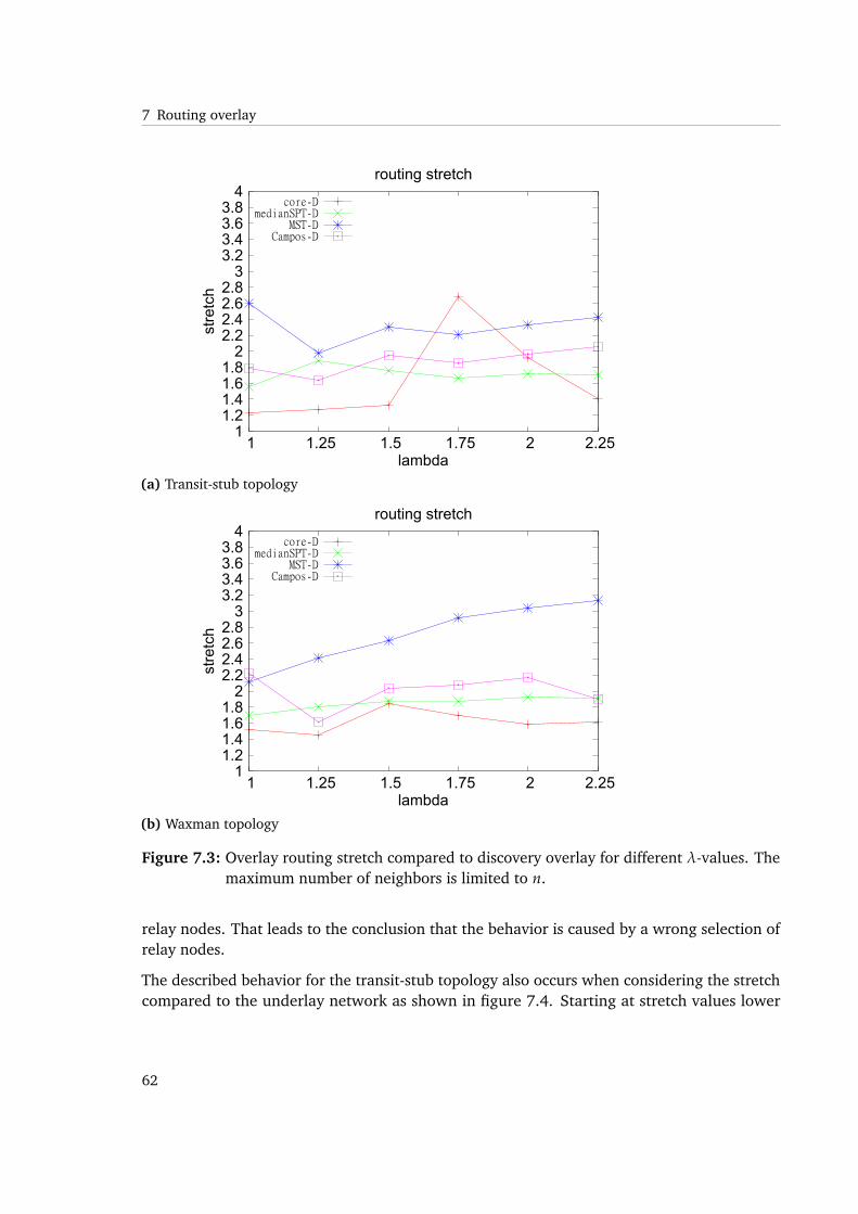
7 Routing overlay
1 1.2 1.4 1.6 1.8
2 2.2 2.4 2.6 2.8
3 3.2 3.4 3.6 3.8
4
1 1.25 1.5 1.75 2 2.25
stre
tch
lambda
routing stretch
core-DmedianSPT-D
MST-DCampos-D
(a) Transit-stub topology
1 1.2 1.4 1.6 1.8
2 2.2 2.4 2.6 2.8
3 3.2 3.4 3.6 3.8
4
1 1.25 1.5 1.75 2 2.25
stre
tch
lambda
routing stretch
core-DmedianSPT-D
MST-DCampos-D
(b) Waxman topology
Figure 7.3: Overlay routing stretch compared to discovery overlay for different λ-values. Themaximum number of neighbors is limited to n.
relay nodes. That leads to the conclusion that the behavior is caused by a wrong selection ofrelay nodes.
The described behavior for the transit-stub topology also occurs when considering the stretchcompared to the underlay network as shown in figure 7.4. Starting at stretch values lower
62
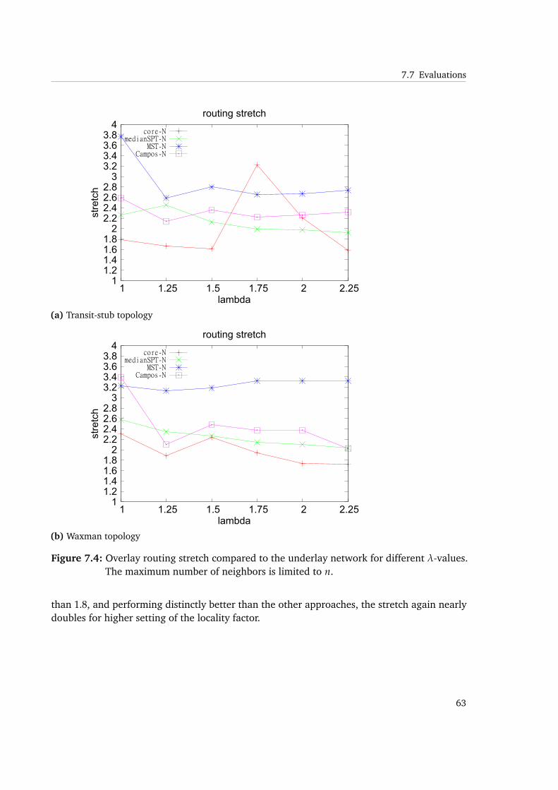
7.7 Evaluations
1 1.2 1.4 1.6 1.8
2 2.2 2.4 2.6 2.8
3 3.2 3.4 3.6 3.8
4
1 1.25 1.5 1.75 2 2.25
stre
tch
lambda
routing stretch
core-NmedianSPT-N
MST-NCampos-N
(a) Transit-stub topology
1 1.2 1.4 1.6 1.8
2 2.2 2.4 2.6 2.8
3 3.2 3.4 3.6 3.8
4
1 1.25 1.5 1.75 2 2.25
stre
tch
lambda
routing stretch
core-NmedianSPT-N
MST-NCampos-N
(b) Waxman topology
Figure 7.4: Overlay routing stretch compared to the underlay network for different λ-values.The maximum number of neighbors is limited to n.
than 1.8, and performing distinctly better than the other approaches, the stretch again nearlydoubles for higher setting of the locality factor.
63

7 Routing overlay
In the Waxman topology again the stretch on the underlay is slightly higher compared totransit-stub, ranging from about 1.75 to 2.3. The same is valid for stretch on the discoveryoverlay, ranging from 1.4 to 1.8.
We will extent simulations on the same topologies, by limit maxN to a more reasonable settingof√
n.
Considering the transit-stub topology, the stretch on D of the core-based overlay is againlower than that of the other approaches for λ < 1.75. We can observe that the same holds forthe stretch on the underlay network, which is obviously higher. The observed effect is againoccurring for λ ≥ 2. The discovery overlay should clearly focus on locality when running thecore-based approach.
For Waxman topologies the improvement over the other approaches is - similar to transit-stub -given for smaller values of λ ≤ 1.5. The achieved improvement in stretch is not that distinct asin transit-stub topologies with unbounded number of neighbors, but still the approach yieldsthe best results of all.
7.7.3 Summary of results
Overall, we can suggest that the discovery overlay should focus on locality when running thecore-based approach. We have shown in simulations, that for values of λ < 1.5 the approachoutperforms all other approaches on both topologies under these conditions.
7.8 Upper and lower bounds on cost and stretch
We will first investigate to what extent upper and lower bounds of overall routing cost andstretch are determined by the core-based structure of the routing overlay. Bounds and approxi-mation ratios on MRCTs were extensively researched by Wu, Chao, Tang et al. [29, 28].
We are considering lower bounds first. All distances on the routing overlay are obviously atleast as high as the distances in the discovery overlay, since R is a subgraph of D. So, for allu, r ∈ PD, dR(u, v) ≥ dD(u, v) holds. A trivial lower bound of the overall routing cost on R canbe given by:
c(R) = ∑u,v∈PD
dR(u, v)
≥ ∑u,v∈PD
dD(u, v)
64
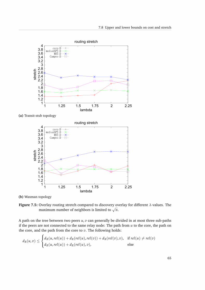
7.8 Upper and lower bounds on cost and stretch
1 1.2 1.4 1.6 1.8
2 2.2 2.4 2.6 2.8
3 3.2 3.4 3.6 3.8
4
1 1.25 1.5 1.75 2 2.25
stre
tch
lambda
routing stretch
core-DmedianSPT-D
MST-DCampos-D
(a) Transit-stub topology
1 1.2 1.4 1.6 1.8
2 2.2 2.4 2.6 2.8
3 3.2 3.4 3.6 3.8
4
1 1.25 1.5 1.75 2 2.25
stre
tch
lambda
routing stretch
core-DmedianSPT-D
MST-DCampos-D
(b) Waxman topology
Figure 7.5: Overlay routing stretch compared to discovery overlay for different λ-values. Themaximum number of neighbors is limited to
√n.
A path on the tree between two peers u, v can generally be divided in at most three sub-pathsif the peers are not connected to the same relay node: The path from u to the core, the path onthe core, and the path from the core to v. The following holds:
dR(u, v) ≤
dR(u, rel(u)) + dR(rel(u), rel(v)) + dR(rel(v), v), if rel(u) 6= rel(v)
dR(u, rel(u)) + dR(rel(u), v), else
65
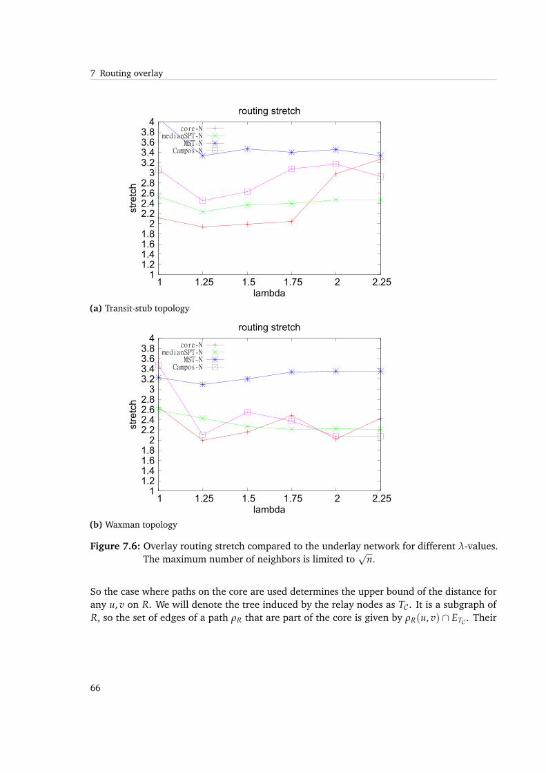
7 Routing overlay
1 1.2 1.4 1.6 1.8
2 2.2 2.4 2.6 2.8
3 3.2 3.4 3.6 3.8
4
1 1.25 1.5 1.75 2 2.25
stre
tch
lambda
routing stretch
core-NmedianSPT-N
MST-NCampos-N
(a) Transit-stub topology
1 1.2 1.4 1.6 1.8
2 2.2 2.4 2.6 2.8
3 3.2 3.4 3.6 3.8
4
1 1.25 1.5 1.75 2 2.25
stre
tch
lambda
routing stretch
core-NmedianSPT-N
MST-NCampos-N
(b) Waxman topology
Figure 7.6: Overlay routing stretch compared to the underlay network for different λ-values.The maximum number of neighbors is limited to
√n.
So the case where paths on the core are used determines the upper bound of the distance forany u, v on R. We will denote the tree induced by the relay nodes as TC . It is a subgraph ofR, so the set of edges of a path ρR that are part of the core is given by ρR(u, v) ∩ ETC . Their
66

7.8 Upper and lower bounds on cost and stretch
contribution to the distance is calculated by the summed weight of all edges that are part ofthe core when using a shortest path from u to v:
dTC (u, v) = ∑e∈ρR(u,v)∩ETC
ωD(e)
Summing up the upper distance bounds of dR for all pairs of peers, we get an upper bound ofthe overall routing cost by [28]:
c(R) = ∑u,v∈PD
dR(u, v)
≤ ∑u,v∈PD
dR(u, rel(u)) + dR(rel(u), rel(v)) + dR(rel(v), v)
≤ ∑u,v∈PD
dR(u, rel(u)) + dR(rel(v), v) + ∑u,v∈PD
dTC (u, v)
≤ 2|PD| ∑u∈PD
dR(u, rel(u)) + ∑u,v∈PD
dTC (u, v)
Consider the first sum-term of that inequality. Since for all non-core peers u the path to rel(u)is the same as the shortest path on the discovery overlay, we can substitute dR(u, rel(u)) in theabove inequality by dD(u, rel(u)), giving:
c(R) ≤ 2|PD|∑u∈PDdD(u, rel(u)) + ∑u,v∈PD
dTC (u, v)
The second sum term, representing the sub-paths through the core, cannot be substitutedaccordingly, as we do not know the exact structure of the core. But we can derive bounds onthe routing load of all edges of the routing overlay e ∈ ER.
Removing e from ER would result in two subtrees. The set of vertices would be given byP′D(e) and PD \ P′D(e). We set x = |P′D(e)|, then, the routing load of e is given by ld(e) =
2x(|PD| − x) = 2|PD|x− 2x2, where x is an integer and x ∈ [1, (|PD| − 1)]. So, we are able toconclude that:
∀e ∈ ER : (ldR(e) ≥ 2(|PD| − 1)) ∧ (ldR(e) ≤|PD|2
2)
So we can give an upper bound for the contribution of the core by [28]:
∑u,v∈PD
dTC (u, v) = ∑e∈ETC
ldR(e)ωD(e)
≤ |PD|2
2 ∑e∈ETC
ωD(e)
67
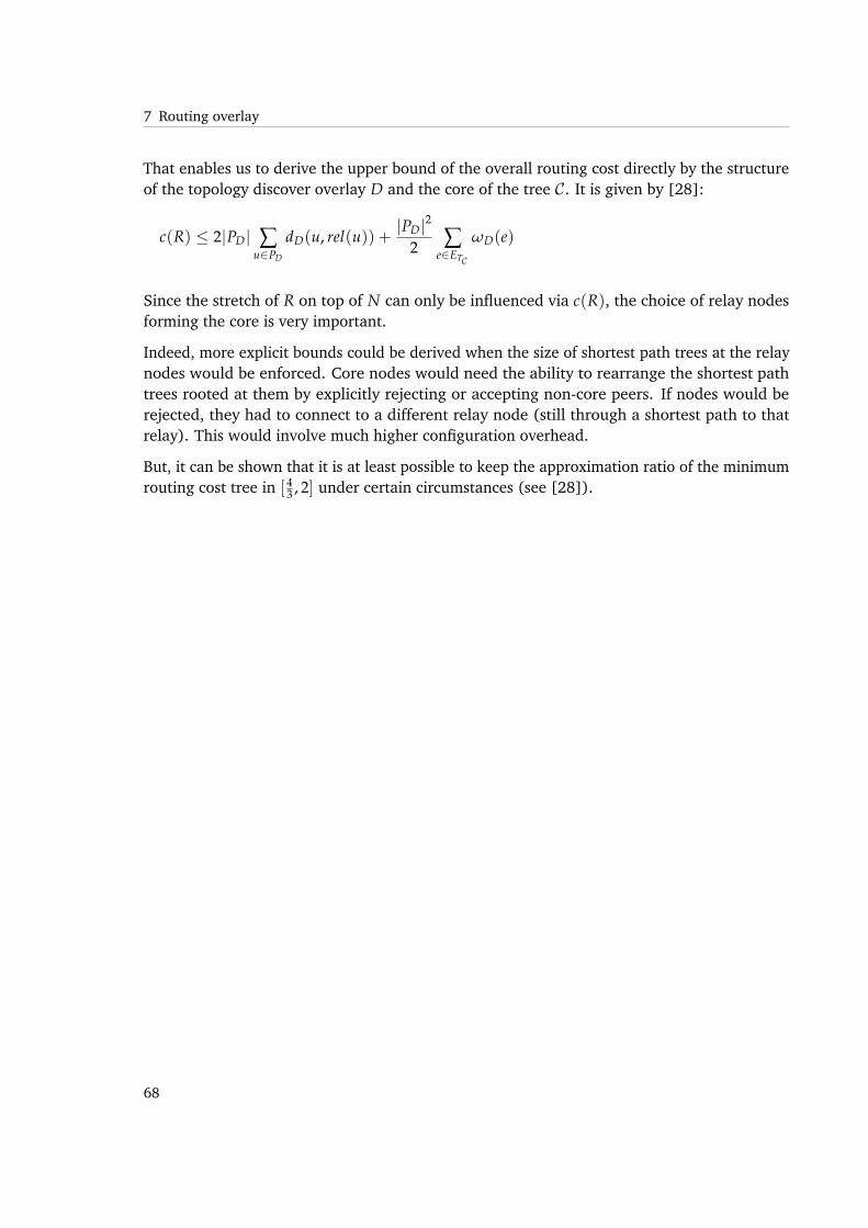
7 Routing overlay
That enables us to derive the upper bound of the overall routing cost directly by the structureof the topology discover overlay D and the core of the tree C. It is given by [28]:
c(R) ≤ 2|PD| ∑u∈PD
dD(u, rel(u)) +|PD|2
2 ∑e∈ETC
ωD(e)
Since the stretch of R on top of N can only be influenced via c(R), the choice of relay nodesforming the core is very important.
Indeed, more explicit bounds could be derived when the size of shortest path trees at the relaynodes would be enforced. Core nodes would need the ability to rearrange the shortest pathtrees rooted at them by explicitly rejecting or accepting non-core peers. If nodes would berejected, they had to connect to a different relay node (still through a shortest path to thatrelay). This would involve much higher configuration overhead.
But, it can be shown that it is at least possible to keep the approximation ratio of the minimumrouting cost tree in [ 4
3 , 2] under certain circumstances (see [28]).
68
8 Conclusion and future work
8.1 Conclusion
We studied the problem of establishing an efficient underlay-aware routing mechanism in thecontext of event dissemination in content-based publish/subscribe overlays. A multi-overlayapproach that divides the problem into sub-problems and conquers them separately wasdeveloped. Another benefit of that technique is that single components of the approach arereusable or can be exchanged. Our work leads to multiple contributions:
1. We proposed a new topology inference scheme that generates an accurate representationof the underlying router-level network using a new distributed algorithm. The scheme isconfigurable via parameters to limit space usage, message overhead and to control its focus onlocality which turned out to be important for our routing approach. We showed in simulationsthat it performs well on different types of Internet-like network topologies and that the emergedpeer-to-peer overlay exhibits low stretch. As a side-effect, underlay link stress is reduced. It ispossible to reach stretch values less than 7% higher than underlay routing. Even when limitingthe local space on each peer to O(
√n) stretches lower than 1.5 can be reached with about
10% of traceroute executions necessary compared to an n-by-n approach.
2. A new routing mechanism that focuses on reducing overall cost between the peers byapproximating an minimum routing cost tree was introduced. The distributed algorithmdetects a high-load subgraph of the routing overlay, which we called the core. We are able toconnect peers through shortest path to the core and showed in simulations that it is possible toachieve reasonable underlay stretch. We compared the results to different other spanning treealgorithms where it performs very well as long as the discovery overlay focuses on locality.
3. We showed how the derived structure can provide underlay-awareness to a content-basedpublish/subscribe systems that benefits from the focus on routing cost minimization.
8.2 Future work
We focused on end-to-end delay as cost metric for the routing overlay throughout this work.With a slight enhancement, it is possible to add support for all sorts of constraints. Assume, weare also given the requirement r(p, q) for each pair of peers. We redefine the communication
69

8 Conclusion and future work
cost to be the path length between the two peers on R multiplied by the requirement. The aimis approximating the spanning tree with the minimum communication cost. That problem iscalled the optimum communication spanning tree (OCT) problem, which is a generalization ofthe MRCT problem [28].
70
Bibliography
[1] B. Awerbuch, “Complexity of network synchronization,” J. ACM, vol. 32, no. 4, pp.804–823, 1985. (Cited on page 55)
[2] B. Awerbuch, “Optimal distributed algorithms for minimum weight spanning tree, count-ing, leader election, and related problems,” Proceedings of the nineteenth annual ACMsymposium on Theory of computing (STOC ’87), 1987. (Cited on pages 49, 54 and 60)
[3] P. Barford, A. Bestavros, J. Byers, and M. Crovella, “On the marginal utility of networktopology measurements,” Proceedings of the 1st ACM SIGCOMM Workshop on InternetMeasurement (IMW ’01), 2001. (Cited on pages 42, 43 and 44)
[4] A. Broido and K. C. Claffy, “Internet Topology: connectivity of IP graphs,” Proceedingsfrom the SPIE International Symposium on Convergence of IT and Communication, pp.172–187, 2001. (Cited on page 42)
[5] M. Bui, F. Butelle, and C. Lavault, “A distributed algorithm for constructing a minimumdiameter spanning tree,” Journal of Parallel and Distributed Computing, vol. 64, no. 5, pp.571–577, 2004. (Cited on page 58)
[6] R. Campos and M. Ricardo, “A fast algorithm for computing minimum routing costspanning trees,” Computer Networks, vol. 52, no. 17, pp. 3229–3247, 2008. (Cited onpages 14, 50, 51 and 61)
[7] K. Chao. (2006) Minimum Routing Cost Spanning Trees. [Online]. Available:http://www.csie.ntu.edu.tw/~kmchao/tree06spr/mrct.ppt (Cited on pages 5 and 50)
[8] M. Faloutsos, P. Faloutsos, and C. Faloutsos, “On power-law relationships of the Internettopology,” Proceedings of the conference on Applications, technologies, architectures, andprotocols for computer communication (SIGCOMM’99), pp. 251–262, 1999. (Cited onpage 30)
[9] R. G. Gallager, P. A. Humblet, and P. M. Spira, “A Distributed Algorithm for Minimum-Weight Spanning Trees,” ACM Transactions on Programming Languages and Systems(TOPLAS), vol. 5, no. 1, pp. 66–77, 1983. (Cited on page 49)
[10] J. A. Garay, S. Kutten, and D. Peleg, “A SubLinear Time Distributed Algorithm forMinimum-Weight Spanning Trees,” SIAM Journal on Computing, vol. 27, no. 1, p. 302,1998. (Cited on page 60)
71
Bibliography
[11] M. R. Garey and D. S. Johnson, Computers and Intractability: A Guide to the Theory ofNP-Completeness, ser. Series of Books in the Mathematical Sciences. W.H.Freeman & Co,1979. (Cited on pages 13 and 50)
[12] M. A. Jaeger, H. Parzyjegla, G. Mühl, and K. Herrmann, “Self-organizing broker topologiesfor publish/subscribe systems,” Proceedings of the 2007 ACM symposium on Appliedcomputing (SAC ’07), 2007. (Cited on page 11)
[13] X. Jin, W. Tu, and S.-H. G. Chan, “Scalable and Efficient End-to-End Network TopologyInference,” IEEE Transactions on Parallel and Distributed Systems, vol. 19, no. 6, pp.837–850, 2008. (Cited on page 13)
[14] D. S. Johnson, J. K. Lenstra, and A. H. G. Rinnooy Kan, “The complexity of the networkdesign problem,” Networks, vol. 8, no. 4, pp. 279–285, 1978. (Cited on page 13)
[15] E. Korach, D. Rotem, and N. Santoro, “Distributed algorithms for finding centers andmedians in networks,” ACM Trans. Program. Lang. Syst, vol. 6, no. 3, pp. 380–401, 1984.(Cited on page 51)
[16] M. Kwon and S. Fahmy, “Path-aware overlay multicast,” Computer Networks, vol. 47,no. 1, pp. 23–45, 2005. (Cited on pages 13 and 20)
[17] C. P. Low and X. Song, “On Finding Feasible Solutions for the Delay Constrained GroupMulticast Routing Problem,” IEEE Transactions on Computers, vol. 51, no. 5, pp. 581–588,2002. (Cited on page 12)
[18] A. Majumder, N. Shrivastava, R. Rastogi, and A. Srinivasan, “Scalable Content-Based Rout-ing in Pub/Sub Systems,” Proceedings of the 28th Conference on Computer Communications(INFOCOM 2009), pp. 567–575, 2009. (Cited on page 11)
[19] A. Medina, A. Lakhina, I. Matta, and J. Byers. (2001) BRITE: UniversalTopology Generation from a User’s Perspective. [Online]. Available: http://www.cs.bu.edu/brite/publications/usermanual.pdf (Cited on page 30)
[20] A. Montresor and M. Jelasity, “PeerSim: A Scalable P2P Simulator,” Proceedings of the 9thInt. Conference on Peer-to-Peer (P2P’09), pp. 99–100, 2009. (Cited on page 31)
[21] G. Parmer, R. West, and G. Fry. (2006) Scalable Overlay Multicast TreeConstruction for QoS-Constrained Media Streaming. [Online]. Available: http://cs-pub.bu.edu/faculty/richwest/papers/TR-2006-020.pdf (Cited on page 12)
[22] M. B. Sharma, J. Chen, and S. Iyengar, “Distributed algorithms for locating centers andmedians in communication networks,” Proceedings of the 1992 ACM/SIGAPP symposiumon Applied computing (SAC’92), pp. 808–817, 1992. (Cited on page 51)
[23] G. Siganos, M. Faloutsos, P. Faloutsos, and C. Faloutsos, “Power laws and the AS-levelinternet topology,” IEEE/ACM Trans. Netw, vol. 11, no. 4, pp. 514–524, 2003. (Cited onpage 30)
72
Bibliography
[24] H. Tangmunarunkit, R. Govindan, S. Jamin, S. Shenker, and W. Willinger. (2002)Network Topology Generators: Degree-Based vs. Structural: Technical Report 02-760.[Online]. Available: http://www.cs.usc.edu/research/02-760.pdf (Cited on page 30)
[25] M. A. Tariq, G. G. Koch, B. Koldehofe, I. Khan, and K. Rothermel, “Dynamic publish/sub-scribe to meet subscriber-defined delay and bandwidth constraints,” Proceedings of theSixteenth International Conference on Parallel Computing (EURO-PAR), 2010. (Cited onpage 11)
[26] B. M. Waxman, “Routing of Multipoint Connections,” IEEE Journal on Selected Areas inCommunications, vol. 6, no. 9, pp. 1617–1622, 1988. (Cited on page 30)
[27] R. T. Wong, “Worst-Case Analysis of Network Design Problem Heuristics,” SIAM Journalon Algebraic and Discrete Methods, vol. 1, pp. 51–63, 1980. (Cited on page 50)
[28] B. Y. Wu and K. M. Chao, Spanning trees and optimization problems. Boca Raton, FL:Chapman & Hall/CRC, 2004. (Cited on pages 13, 14, 50, 52, 54, 64, 67, 68 and 70)
[29] B. Y. Wu, K. M. Chao, and C. Y. Tang, “Approximation algorithms for the shortest totalpath length spanning tree problem,” Discrete Applied Mathematics, vol. 105, no. 1-3, pp.273–289, 2000. (Cited on pages 13 and 64)
[30] E. W. Zegura, “Modeling Internet Topology,” 2002. (Cited on page 30)
[31] E. W. Zegura, K. L. Calvert, and S. Bhattacharjee, “How to Model an Internetwork,” Pro-ceedings of the Fifteenth Annual Joint Conference of the IEEE Computer and CommunicationsSocieties (INFOCOM 1996), pp. 594–602, 1996. (Cited on page 30)
[32] E. Zegura. (2000) Modeling Topology of Large Internetworks. [Online]. Available:http://www.cc.gatech.edu/projects/gtitm/ (Cited on page 30)
[33] Y. Zhu and B. Li, “Correlation-Aware Multimedia Content Distribution in Overlay Net-works,” Proceedings of the Thirteenth Annual SPIE/ACM Conference on Multimedia Com-puting and Networking (MMCN 2006), pp. 127–138, 2006. (Cited on page 12)
[34] Y. Zhu and B. Li, “Overlay Networks with Linear Capacity Constraints,” IEEE Transactionson Parallel and Distributed Systems, vol. 19, no. 2, pp. 159–173, 2008. (Cited on page 12)
All links were last followed on August 3, 2011.
73


Declaration
All the work contained within this thesis,except where otherwise acknowledged, wassolely the effort of the author. At nostage was any collaboration entered intowith any other party.
(Christian Schieberle)