251

International Journal of Mechanical and Materials Engineering (IJMME), Vol. 7 (2012), No. 3, 251-258.

UNDERHOOD GEOMETRY MODIFICATION AND TRANSIENT COOLANT

TEMPERATURE MODELLING FOR ROBUST COOLING NETWORKS

S.C. Pang*, M.A. Kalam, H.H.Masjuki, I.A. Badruddin, R. Ramli and M.A. Hazrat

Department of Mechanical Engineering, University of Malaya, 50603 Kuala Lumpur, Malaysia

*Corresponding author’s E-mail: psuhchyn@yahoo.com

Received 11 January 2013, Accepted 15 January 2013

ABSTRACT

In this current era, increasing computing power, effort to

reduce prototypes’ cost and time, and shorten design-to-

product time urges the need of numerical computation.

Higher cooling’s load or requirement is attributed by

higher power of engine. Also, higher quantity of heat

exchangers and vehicles’ styling resulted limited space at

vehicles’ hood. These factors have caused the design job

of vehicles’ hood and engine cooling system to be more

crucial and challenging. A well designed and robust

engine cooling system could sustain in the worst and

toughest condition. One of the worst conditions for

engine cooling system is sudden keying-off of engine

after hill climbing and high speed driving. In this

research, three dimensional computational fluids

dynamic (CFD) is utilised to model the dynamic air flow

at the hood with complicated geometry. On the other

hand, one dimensional thermo-fluid model could

simulate the system effect after including all the

components in engine cooling system. With integration

of both models, the transient coolant temperature before

and after vehicles’ keying off is simulated and is

analysed thoroughly. Front-end hood geometry is

morphed to reduce air separation at heat exchangers.

Two cone-shaped air directing devices are included to

guide higher volume of ram air toward frontal face of

heat exchangers. Different heat soak scenarios are

simulated and transient temperature trend is observed.

The coolant temperature tends to increase tremendously

when huge amount of heat soak could not be dissipated

away in-time.

Keywords: Basic engine cooling system, Transient, Heat

soak, Keying-off, Geometry modification.

Nomenclature

Abbreviations and Acronyms

C: Porous viscous resistance [kg/m3s]

D: Porous inertial resistance [kg/m4]

F: Corrections factor

V: Velocity [m/s]

ΔP: Pressure drop [Pa]

L: Length [m]

Re: Reynolds number

DH: Hydraulic diameter, coolant and air sides [m]

A: Reference area, for coolant and air sides [m2]

m: Mass flow rates, for coolant and air sides [kg/s]

μ: Dynamic viscosity [kg/ m s]

U: Overall heat transfer coefficient [W/ m2K]

x: Radiator thickness [m]

K: Thermal conductivity for coolant and air [W/ m K]

Cp: Specific heat, for coolant and air [J/ kg K]

ε: Radiator efficiency [%]

1. INTRODUCTION

Increasing computing power, effort to reduce prototypes’

cost and time, and shorten design-to-product time urges

the need of numerical computation. The design of the

vehicles’ cooling system mainly includes cooling air

flow path and coolant flow path. The cooling air flow

will pass through the front bumper, grille, other heat

exchangers etc., the velocity distribution at the face of

radiator is highly non-uniform, especially in low speed

driving. In this research, computational fluid dynamics

model is developed to simulate the dynamics air flow to

radiator. The three dimensional CFD model could

capture the air flow throughput to radiator which will be

fed into the thermo-fluid model later. CFD model also

allows geometry modifications to be carried out in order

to improve air flows’ throughput and distribution to

radiator. Secondly, a thermo-fluid model is established to

simulate the coolant flow circuit especially the transient

coolant temperature after vehicles’ keying off. Different

heat soak scenarios after vehicles’ keying off are

simulated in the thermo-fluid model.

In order to capture the geometry effect, the vehicle’s

under-hood dynamic air flow is always modelled using

CFD. In the literature, in order to study the velocity

profile and temperature distribution, the steady state

cooling air flow path has been modelled with simplified

under-hood geometry in StarCD using SIMPISO solver.

The numerical model was validated with experimental

results from a wind tunnel (Zyl, 2006). For other

applications, a cooling fan and heat shield were designed

and the distance between the fan and heat exchanger was

optimized for a heavy-duty truck using CFD (Mao et al.,

2010). Also, the air velocity across the radiator’s frontal

surface and the air-to-boil temperature were calculated

by a CFD model using PASSAGE (Ecer et al., 1995). A

thought- provoking investigation using a computational

procedure was carried out and was implemented in

VECTIS. The research studied under-hood thermal

management and the proposed procedure delivers

accurate transient predictions in substantially reduced

computational time (Franchetta et al., 2007). Several

geometry modifications were performed in the StarCD

CFD model to improve the air flow approaching the

intercooler (Lawrence, 2001). On the other hand, a

combination of CFD and Flow Network Modelling

252

instead of a single CFD model is being utilized to model

the under-hood air flow path (Kumar et al., 2009).

To reflect the system effect of the coolant flow path, one-

dimensional thermo-fluid simulation is a better solution.

Some research utilized AMESim to perform system

analysis of an engine cooling system (Ning, 2009). There

was also a case in which the cooling air flow and coolant

flow path were both simulated using one-dimensional

thermo-fluid software, KULI (Eichlseder et al., 1997).

With regard to the coupling of CFD and thermo-fluid

simulation, an industry-based expert integrated StarCD

and Flowmaster for passenger cabin cooling analysis

(Rok and Pasthor, 2007). Researchers also coupled

Fluent, StarCD, and KULI for automotive air

conditioning analysis including the air flow approaching

the condenser (Kim and Kim, 2008). Extensive

experiment-based research was also conducted to control

car under-hood thermal conditions. An innovative and

accurate method to measure under-hood radiative and

convective heat flux was proposed in the research.

Optimized thermal management through proper

positioning of the components (upstream and

downstream) and placing of the deflector was also

suggested (Khaled et al., 2010, 2011).

In this research, air flow data through the radiator are

obtained from a CFD model. Some geometry

modifications are carried out to improve the air flow

distribution at the radiator. Later, with the air flow input

from CFD, the transient coolant temperature after the

vehicle is keyed off is modelled. Several keyed-off

scenarios were modelled while varying the heat soak,

such as thermal lagging of 100 s, 200 s, 300 s, and 400 s.

2. NUMERICAL MODELLING

2.1 Three-Dimensional CFD model

In this paper, the under-hood air flow with different

driving conditions was modelled using Star-CCM+ (CD

Adapco, 2010). The main activities which are involved in

a CFD models’ establishment which are import of

geometry, surface meshing, volume meshing and physics

modelling, simulation execution and result analysis.

Firstly, the hood and bonnet geometry was imported into

Star-CCM+. Figure 1(a) shows the geometry of front-

half-car and a bundle of components at the underhood.

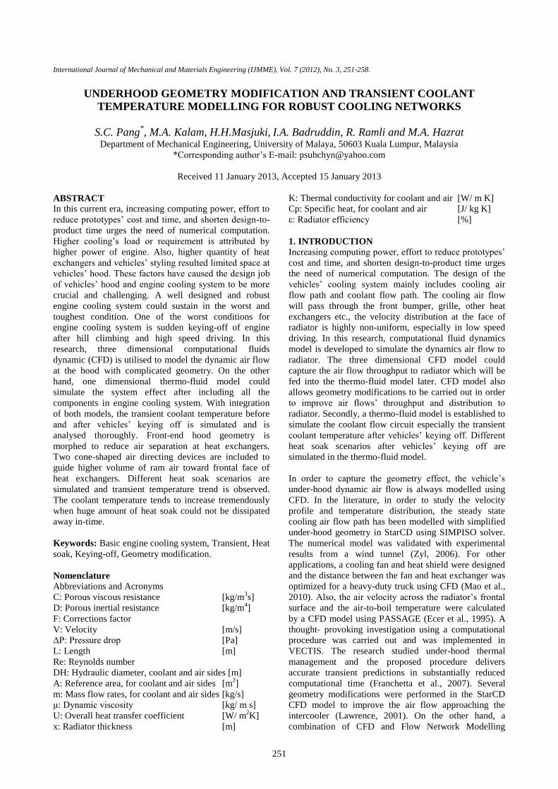
The meshing task is challenging as the components are

placed closely to each other. Figure 1(b) shows that the

main air flow path consists of the condenser, radiator,

fan, shroud, and engine body. During the surface

meshing stage, the mesh size, feature curve, multiple

regions, and boundaries were defined. Table 1 shows the

surface mesh size of some significant parts. For parts

which require accurate and detailed flows, a smaller

mesh size is preferable. However, it was not necessary to

waste additional computational time and effort by

assigning a small mesh size to all parts (i.e., the wind

tunnel). Thirdly, polyhedral and prism-layer mesh types

were selected for volume meshing. In this model, the

volume mesh comprised a total of 7,760,056 volume

cells.

In the stage of physics modelling, the initial and

boundary conditions are defined; interfaces are created

between regions; region types are defined; and the

physics continuum is selected. In selecting the physics

continuum, decisions are made for viscous scheme

(laminar or turbulent), flow type (segregated or coupled),

turbulence model, space, time, and equation of state. One

important aspect in modelling was the setting of

interfaces between regions. There were a total of eight

regions in this model and the main region was the free

stream. The interface will be created between two

regions where two similar boundaries (one at each

region) are connected.

Figure 1 (a) Meshing of Vehicle Front End and Under-

Hood. (b) Mesh Scene of Under-hood Heat Exchangers,

Shroud, Fan, and Engine Body.

Table 1 Mesh Size of Important Boundaries.

Boundary Mesh Size (mm)

Bumper 5 mm

Grille 1 mm

Radiator core 4 mm

Condenser 4 mm

Fan blade 2 mm

Fan cylinder 5 mm

Shroud 3 mm

Wind tunnel 20 mm

Engine body 5 mm

Exhaust Parts 5 mm

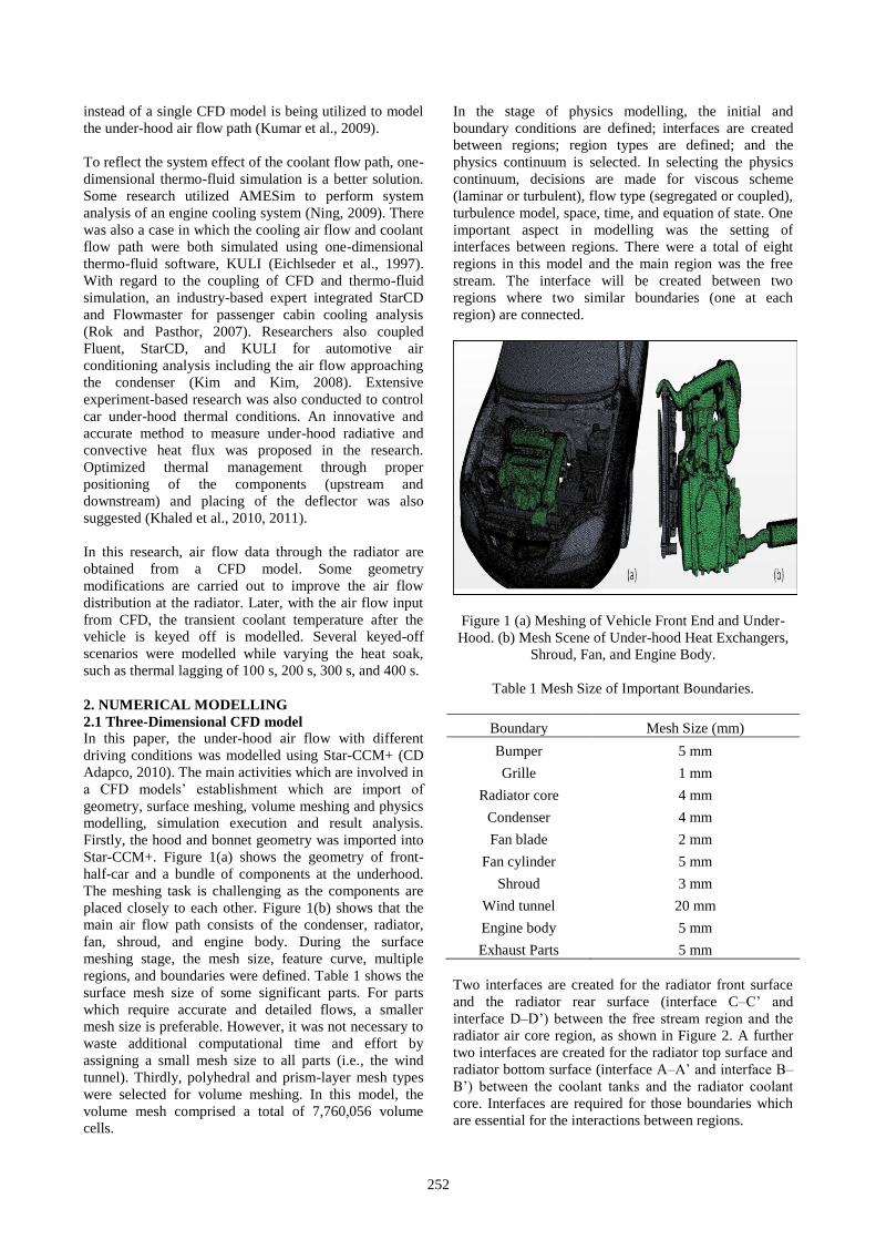
Two interfaces are created for the radiator front surface

and the radiator rear surface (interface C–C’ and

interface D–D’) between the free stream region and the

radiator air core region, as shown in Figure 2. A further

two interfaces are created for the radiator top surface and

radiator bottom surface (interface A–A’ and interface B–

B’) between the coolant tanks and the radiator coolant

core. Interfaces are required for those boundaries which

are essential for the interactions between regions.

253

The porosity of the heat exchanger towards the fluid flow

is defined by porous media method. Table 2 shows the

data of pressure drop versus air velocity for radiator air

flow. With linear regression, the value for porous viscous

resistance and porous inertial resistance of radiator air

flow could be obtained (Eq. (1)). As the values of

pressure drop versus fluid velocity are available,

constants C and D can be obtained by linear regression.

Constant C represents the porous viscous resistance and

constant D the porous inertial resistance for a porous

medium.

(1)

Table 2 Porous Resistance Obtained with Linear

Regression, for Radiator Air Flow.

Pressure drop/Length

[Pa/m]

Velocity

[m/s]

Velocity2

[m2/s

2]

1,250 2 4

3,438 4 16

6,563 6 36

11,250 8 64

16,875 10 100

Figure 2 Interfaces Created at Radiator Core (Interface

A–A’, Interface B–B’, Interface C–C’, Interface D–D’).

The radiator was modelled as a dual stream heat

exchanger with the involvement of two heat transfer

fluids. Thus, two set of flow resistance values are

required for the radiator, one for air flows horizontally in

the x-direction and another for coolant flows vertically in

the z-direction. To elaborate the modelling of the dual

stream heat exchanger, one radiator core was duplicated

after volume meshing. One radiator core was the air

continuum; another radiator core was the coolant

continuum. A heat exchanger’s interface will be created

and activated between the two radiator cores. Moreover,

it is required to define each of the porous resistance in

vector form [i, j, k]. This means that it is direction

sensitive. The direction of the porous resistance is

defined either in the x- axis, y- axis or z- axis. For

instance, radiator air can flow through radiator in x-

direction, and the porous viscous resistance is [279.60

kg/m4, 1000000 kg/m

4, 1000000 kg/m

4]. High value of

porous resistance in y and z- direction means that high

resistance of air flow toward particular directions. On the

other hand, the radiator coolant can flow through radiator

in z-direction; the porous viscous resistance is [1000000

kg/m4, 1000000 kg/m

4, 74945 kg/m

4].

The condenser was modelled as a single stream heat

exchanger, and only one type of fluid is participating.

The condenser was modelled as a porous medium for air

flow, using the method illustrated earlier. The heat

exchanger’s upstream (front) and downstream (rear)

boundaries were determined. Other values like the heat

exchanger energy transfer, heat exchanger minimum

temperature difference, and heat exchanger temperature

were tuned.

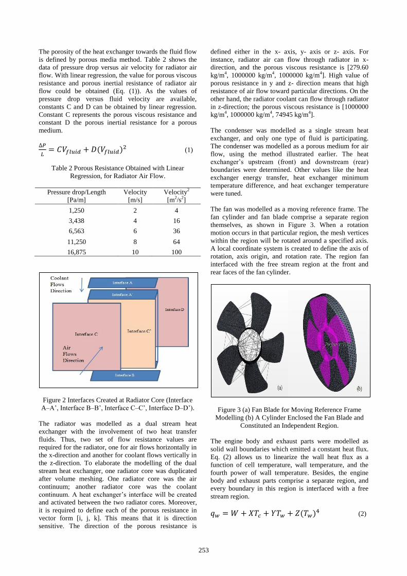
The fan was modelled as a moving reference frame. The

fan cylinder and fan blade comprise a separate region

themselves, as shown in Figure 3. When a rotation

motion occurs in that particular region, the mesh vertices

within the region will be rotated around a specified axis.

A local coordinate system is created to define the axis of

rotation, axis origin, and rotation rate. The region fan

interfaced with the free stream region at the front and

rear faces of the fan cylinder.

Figure 3 (a) Fan Blade for Moving Reference Frame

Modelling (b) A Cylinder Enclosed the Fan Blade and

Constituted an Independent Region.

The engine body and exhaust parts were modelled as

solid wall boundaries which emitted a constant heat flux.

Eq. (2) allows us to linearize the wall heat flux as a

function of cell temperature, wall temperature, and the

fourth power of wall temperature. Besides, the engine

body and exhaust parts comprise a separate region, and

every boundary in this region is interfaced with a free

stream region.

(2)

254

2.2 One-Dimensional thermo-fluid model

One dimensional thermo-fluid simulation is always

utilised to study and to investigate the system effect of

engine cooling circuit, lubrication circuit, transmission

circuit, HVAC system and other thermo- hydraulic

system in vehicles. In this research, software called

Flowmaster (2010) is used and the study is focused on

engine cooling system. There are numerous components

in the coolant circuit. The components consist of heat

exchangers, pipes, valve, thermostat, heat source,

pressure source, flow source, expansion tank, pump,

gauge etc. After drag-and-drop the components into

circuit, the components are linked together in a loop. It

mimics an electronic circuit with different electronic

components. The model built is used to study individual

component’s effect onto the whole engine cooling system

and the interactions between components. Then, it is

required to set parameters of each and every component

in details. For the radiator, the parameters are coolant

flow area, coolant hydraulic diameter, airside flow area,

airside hydraulic diameter, curve of coolant side pressure

drop versus flow rates, curve of airside pressure drop vs.

flow rates etc.

For the radiator, the surface of the heat transfer versus air

flow versus coolant flow was available at a determined

inlet temperature difference. The heat transfer surface

was normalized and converted to a Nusselt surface [Nu

vs. Re (air) vs. Re (coolant)], by applying Eqs. 3–13

(Flowmaster Limited, 2010). Eqs. (3) and (4) normalized

coolant flow and air flow to their respective Reynolds

numbers. As the value of heat transferred, air inlet

temperature, and coolant outlet temperature were known,

the air outlet temperature and coolant outlet temperature

could be computed by Eqs. (5) and (6). As the fluid

temperatures were all known, the log mean temperature

difference (LMTD) could be computed. After this, Eq.

(7) can be used to calculate the overall heat transfer

coefficient. With Eq. (8), the overall heat transfer

coefficient was normalized to the Nusselt number. Eq.

(9) shows the relationship between the maximum heat

dissipation (mCp)min and the fluids inlet temperature

difference (ITD). Eq. (10) was used to calculate the

effectiveness of the heat exchanger. Eqs. (11) and (12)

indicate the effectiveness as a function of fluid

temperatures. Eq. (13) indicates the constraints whereby

the coolant outlet temperature must be greater than the

air inlet temperature and the coolant inlet temperature

must be greater than the air outlet temperature.

(3)

(4)

( ) (5)

( ) (6)

(7)

( ) ( )

( )

( )

(8)

( ) (9)

(10)

(11)

(12)

(13)

Figure 4 Input Data of Engine Heat, Coolant Flow, and

Air Flow for the Case with 400 s of Thermal Lagging.

Table 3 Test Scenarios of Different Heat Soak Values

after Keying-off.

Cases Thermal Lag Min. Air/

Coolant Flow

Min. Engine Heat

Case 1 0 s 2800 s 2800 s

Case 2 100 s 2800 s 2900 s

Case 3 200 s 2800 s 3000 s

Case 4 300 s 2800 s 3100 s

Case 5 400 s 2800 s 3200 s

The air flow data obtained from the CFD models and

coolant flow data from industry are incorporated into the

one-dimensional thermo-fluid model for the time

behaviour study. The engine heat, coolant flow, and air

flow are varied over the simulation time horizon. The

vehicle was decreased at 2500 s and keyed off at 2800 s.

The keyed-off time was defined as the time when coolant

flow and air flow reached a minimum. In the basic

scenario with 0 s of thermal lag, the engine heat

decreased concurrently with the air flow (fan) and

coolant flow (water pump). This was the scenario with

the least heat soak. The scenarios were varied with

255

increasing thermal lag and heat soak, as summarized in

Table 3. Finally, Figure 4 shows Case 5, with 400 s of

thermal lag and the highest amount of heat soak. The

heat soak was a result of engine heat that could not be

dissipated away from the engine cooling system. The

coolant peak temperatures were observed for different

scenarios.

3. RESULTS AND DISSCUSSION

3.1 Front end geometry modification

The CFD model was simulated under different driving

conditions in order to obtain the respective air flow

throughputs at the radiator. Table 4 tabulates the

numerical air flow data together with the industry data of

coolant flow. Later, these data will be used as important

inputs into the one-dimensional thermo- fluid model.

CFD is a three-dimensional simulation tool which

emphasizes the effects of geometry on fluid flow. A

complete and detailed under-hood geometry layout

includes the bumper, grille, lamp, lamp box, front end

mechanical structure, bumper beam, transmission box,

condenser, radiator, intake manifold, exhaust manifold,

exhaust catalyst, battery, engine body, and all piping. The

layout of these components will affect the air flow

approaching the condenser and radiator. In high speed

and middle speed driving, the cooling of heat exchangers

depends greatly on ram air, whereas in low speed driving

and vehicle idling, the cooling of heat exchangers

depends on the fan suction from the rear side. In this

model, we simulate the air flow by approaching heat

exchangers with a complete under-hood geometry layout.

At high speed and middle speed driving (> 60 km/hr), the

front end structure, grille, and bumper significantly

influence the air flow distribution on the frontal surface

of the heat exchangers.

Table 4 CFD Radiator Air Flow and Industry Coolant

Flow under Different Driving Conditions.

Ram Air

[km/hr]

Fan

[rpm]

Radiator Air

Flow [kg/s]

Radiator Coolant

Flow [kg/s]

50 50 0.2928 0.79

50 2000 0.4700 0.79

80 0 0.4900 0.97

110 50 0.7904 1.08

160 50 1.2170 1.33

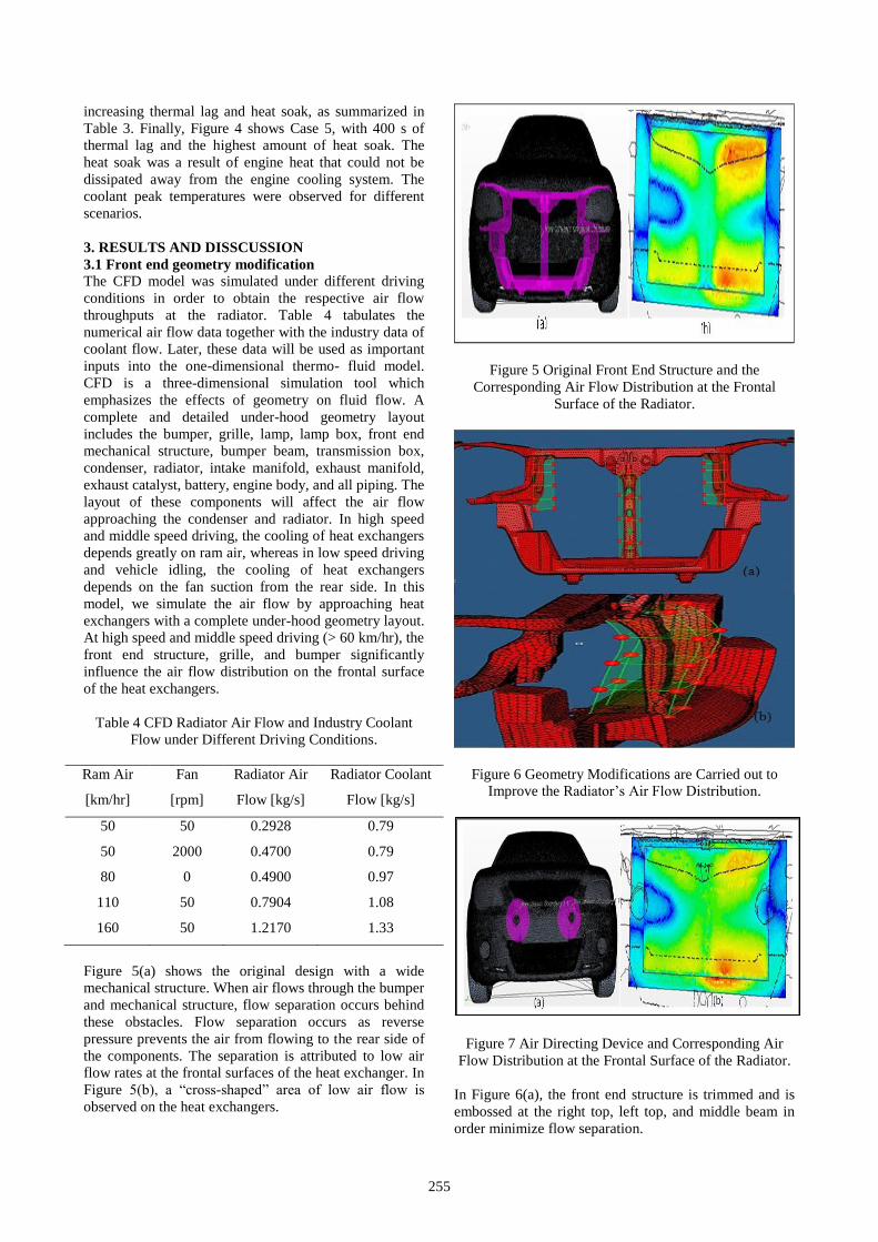
Figure 5(a) shows the original design with a wide

mechanical structure. When air flows through the bumper

and mechanical structure, flow separation occurs behind

these obstacles. Flow separation occurs as reverse

pressure prevents the air from flowing to the rear side of

the components. The separation is attributed to low air

flow rates at the frontal surfaces of the heat exchanger. In

Figure 5(b), a “cross-shaped” area of low air flow is

observed on the heat exchangers.

Figure 5 Original Front End Structure and the

Corresponding Air Flow Distribution at the Frontal

Surface of the Radiator.

Figure 6 Geometry Modifications are Carried out to

Improve the Radiator’s Air Flow Distribution.

Figure 7 Air Directing Device and Corresponding Air

Flow Distribution at the Frontal Surface of the Radiator.

In Figure 6(a), the front end structure is trimmed and is

embossed at the right top, left top, and middle beam in

order minimize flow separation.

256

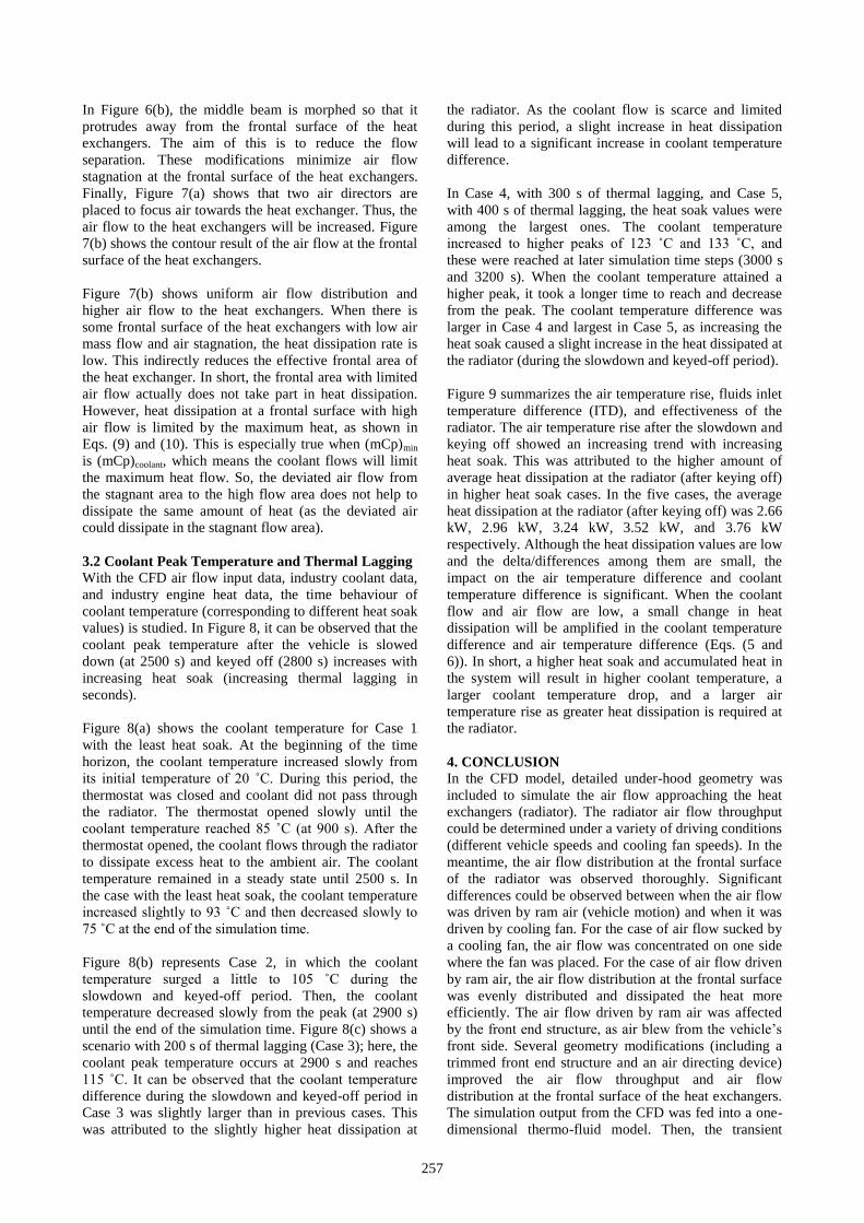
Figure 8 Coolant Temperature within Simulation Time Horizon for All Testing Scenarios.

Figure 9 Air Temperature Rise, Inlet Temperature Difference, and Thermal Effectiveness for All Scenario.

257

In Figure 6(b), the middle beam is morphed so that it

protrudes away from the frontal surface of the heat

exchangers. The aim of this is to reduce the flow

separation. These modifications minimize air flow

stagnation at the frontal surface of the heat exchangers.

Finally, Figure 7(a) shows that two air directors are

placed to focus air towards the heat exchanger. Thus, the

air flow to the heat exchangers will be increased. Figure

7(b) shows the contour result of the air flow at the frontal

surface of the heat exchangers.

Figure 7(b) shows uniform air flow distribution and

higher air flow to the heat exchangers. When there is

some frontal surface of the heat exchangers with low air

mass flow and air stagnation, the heat dissipation rate is

low. This indirectly reduces the effective frontal area of

the heat exchanger. In short, the frontal area with limited

air flow actually does not take part in heat dissipation.

However, heat dissipation at a frontal surface with high

air flow is limited by the maximum heat, as shown in

Eqs. (9) and (10). This is especially true when (mCp)min

is (mCp)coolant, which means the coolant flows will limit

the maximum heat flow. So, the deviated air flow from

the stagnant area to the high flow area does not help to

dissipate the same amount of heat (as the deviated air

could dissipate in the stagnant flow area).

3.2 Coolant Peak Temperature and Thermal Lagging

With the CFD air flow input data, industry coolant data,

and industry engine heat data, the time behaviour of

coolant temperature (corresponding to different heat soak

values) is studied. In Figure 8, it can be observed that the

coolant peak temperature after the vehicle is slowed

down (at 2500 s) and keyed off (2800 s) increases with

increasing heat soak (increasing thermal lagging in

seconds).

Figure 8(a) shows the coolant temperature for Case 1

with the least heat soak. At the beginning of the time

horizon, the coolant temperature increased slowly from

its initial temperature of 20 ˚C. During this period, the

thermostat was closed and coolant did not pass through

the radiator. The thermostat opened slowly until the

coolant temperature reached 85 ˚C (at 900 s). After the

thermostat opened, the coolant flows through the radiator

to dissipate excess heat to the ambient air. The coolant

temperature remained in a steady state until 2500 s. In

the case with the least heat soak, the coolant temperature

increased slightly to 93 ˚C and then decreased slowly to

75 ˚C at the end of the simulation time.

Figure 8(b) represents Case 2, in which the coolant

temperature surged a little to 105 ˚C during the

slowdown and keyed-off period. Then, the coolant

temperature decreased slowly from the peak (at 2900 s)

until the end of the simulation time. Figure 8(c) shows a

scenario with 200 s of thermal lagging (Case 3); here, the

coolant peak temperature occurs at 2900 s and reaches

115 ˚C. It can be observed that the coolant temperature

difference during the slowdown and keyed-off period in

Case 3 was slightly larger than in previous cases. This

was attributed to the slightly higher heat dissipation at

the radiator. As the coolant flow is scarce and limited

during this period, a slight increase in heat dissipation

will lead to a significant increase in coolant temperature

difference.

In Case 4, with 300 s of thermal lagging, and Case 5,

with 400 s of thermal lagging, the heat soak values were

among the largest ones. The coolant temperature

increased to higher peaks of 123 ˚C and 133 ˚C, and

these were reached at later simulation time steps (3000 s

and 3200 s). When the coolant temperature attained a

higher peak, it took a longer time to reach and decrease

from the peak. The coolant temperature difference was

larger in Case 4 and largest in Case 5, as increasing the

heat soak caused a slight increase in the heat dissipated at

the radiator (during the slowdown and keyed-off period).

Figure 9 summarizes the air temperature rise, fluids inlet

temperature difference (ITD), and effectiveness of the

radiator. The air temperature rise after the slowdown and

keying off showed an increasing trend with increasing

heat soak. This was attributed to the higher amount of

average heat dissipation at the radiator (after keying off)

in higher heat soak cases. In the five cases, the average

heat dissipation at the radiator (after keying off) was 2.66

kW, 2.96 kW, 3.24 kW, 3.52 kW, and 3.76 kW

respectively. Although the heat dissipation values are low

and the delta/differences among them are small, the

impact on the air temperature difference and coolant

temperature difference is significant. When the coolant

flow and air flow are low, a small change in heat

dissipation will be amplified in the coolant temperature

difference and air temperature difference (Eqs. (5 and

6)). In short, a higher heat soak and accumulated heat in

the system will result in higher coolant temperature, a

larger coolant temperature drop, and a larger air

temperature rise as greater heat dissipation is required at

the radiator.

4. CONCLUSION

In the CFD model, detailed under-hood geometry was

included to simulate the air flow approaching the heat

exchangers (radiator). The radiator air flow throughput

could be determined under a variety of driving conditions

(different vehicle speeds and cooling fan speeds). In the

meantime, the air flow distribution at the frontal surface

of the radiator was observed thoroughly. Significant

differences could be observed between when the air flow

was driven by ram air (vehicle motion) and when it was

driven by cooling fan. For the case of air flow sucked by

a cooling fan, the air flow was concentrated on one side

where the fan was placed. For the case of air flow driven

by ram air, the air flow distribution at the frontal surface

was evenly distributed and dissipated the heat more

efficiently. The air flow driven by ram air was affected

by the front end structure, as air blew from the vehicle’s

front side. Several geometry modifications (including a

trimmed front end structure and an air directing device)

improved the air flow throughput and air flow

distribution at the frontal surface of the heat exchangers.

The simulation output from the CFD was fed into a one-

dimensional thermo-fluid model. Then, the transient

258

coolant temperature after the vehicle was keyed off was

modelled with different heat soak/thermal lag scenarios.

The scenario with 400 s of thermal lag showed the

highest coolant peak temperature. In order to reduce the

coolant peak temperature after keying-off, prolonged

operation of the water pump and fan is suggested. This

will reduce the heat soak indirectly.

ACKNOWLEDGEMENT

I would like to express my gratitude and appreciation to

the Malaysia Ministry of Science, Technology and

Innovation (TF0608C073) and the Institute of Research

Management and Monitoring of University Malaya

(RG145-12AET). Their financial support enabled us to

conduct the current research.

REFERENCES

CD Adapco. 2010. Star CCM+ (Version 6.02.007).

Ecer, A., Toksoy, C., Rubek, V., Hall, R., Gezmisoglu,

G., Pagliarulo, V. and Azzali, J. 1995. Air Flow and

Heat Transfer Analysis of an Automotive Engine

Radiator to Calculate Air-to-Boil Temperature, SAE

International: SAE Paper 951015.

Eichlseder, W., Raab, G., Hager, J. and Raup, M. 1997.

Use of Simulation Tools with Integrated Coolant

Flow Analysis for the Cooling System Design, SAE

International: SAE Paper 971815.

Flowmaster Limited. 2010. Flowmaster V7.

Franchetta, M., Suen, K. and Bancroft, T. 2007. Pseudo-

transient Computational Fluid Dynamics Analysis of

an Underboonet Compartment during Thermal Soak,

Proceedings of the Institution of Mechanical

Engineers, Part D: Journal of Automobile

Engineering 221 (10): 1209-1220.

Khaled, M., Harambat, F. and Peerhossaini, H. 2010.

Underhood Thermal Management: Temperature and

Heat Flux Measurements and Physical Analysis,

Applied Thermal Engineering 30 (6-7): 590-598.

Khaled, M., Harambat, F. and Peerhossaini, H. 2011.

Towards the Control of Car Underhood Thermal

Conditions, Applied Thermal Engineering 31 (5):

902-910.

Kim, H. J. and Kim, C.J. (2008). A Numerical Analysis

for the Cooling Module related to Automobile Air-

conditioning System, Applied Thermal Engineering

28 (14-15): 1896-1905.

Kumar, V., Kapoor, S., Arora, G. and Dutta, P. 2009. A

Combined CFD and Flow Network Modeling

Approach for Vehicle Underhood Air Flow and

Thermal Analysis, SAE International: SAE Paper

2009-01-1150.

Lawrence, V. 2001. Underhood Airflow Simulation of a

Passenger Car Using Computational Fluid Dynamics,

SAE International: SAE Paper 2001-01-3800.

Mao, S., Feng, Z. and Michaelides, E.E. 2010. Off-

highway Heavy-duty Truck Under-hood Thermal

Analysis, Applied Thermal Engineering 30 (13):

1726-1733.

Ning, G. 2009. Simulation of Engine Cooling System

Based on AMEsim, Paper presented at the 2nd

International Conference on Information and

Computing Science, Manchester, United Kingdom.

Rok, S.H. and Pasthor, H. 2007. A Real Time Numerical

Analysis of Vehicle Cool-down Performance, VTMS

8: ISBN 1843343487.

Zyl, J.M.V. 2006. Numerical Modeling and Experimental

Investigation of the Flow and Thermal Processes in a

Motor Car Vehicle Underhood, Thesis (MScEng,

Mechanical and Mechatronic Engineering),

University of Stellenbosch.