Undergraduate Honors Thesis By Shuhan Li Undergraduate

Undergraduate Honors Thesis

Influence of the Wall Heat Transfer on Flame Propagation

By

Shuhan Li

Undergraduate Program in Department of Mechanical Engineering

The Ohio State University

2016

Dissertation Committee:

Dr. Seung Hyun Kim, advisor

Dr. Shaurya Prakash

Copyright by

Shuhan Li

2016

1

Abstract In the internal combustion engines, the flames interact with the walls of the

cylinder, which affects the flame propagation characteristics and the engine performance.

The flame tends to quench near the wall, which is due to wall heat fluxes. Also, wall heat

transfer can play a significant role in undesirable auto-ignition of unburned mixture in the

cylinder. The flame-unburned mixture-wall interactions can influence engine knock and

affect the engine emission. The present research is aimed at understanding the effects of

wall heat transfer on flame propagation. The flame propagation in the presence of the

walls will be simulated and the effects of wall heat transfer on flame propagation

properties will be investigated by changing wall temperature, pressures, channel widths,

and equivalence ratios. By analyzing variations of those properties, we will be able to

advance an understanding of flame-mixture ignition-wall heat transfer interactions, which

will help reduce engine knock and emission for different types of engine structures. This

research focuses mainly on the propagation of laminar premixed flames. The numerical

method is used to solve the mass, momentum and energy conservation together with the

combustion model. The first stage study focuses on using a single step chemistry reaction

model to simulate flame propagating along one dimensional domain and two dimensional

channels with adiabatic walls under different air fuel ratios, geometries, and injected flow

velocity. This simulation is aimed to provide a reasonable distribution of temperature,

flow velocity, pressure, fuel, oxidizer and products in the presence of the adiabatic walls.

Based on the first stage, the second stage study focuses on adding heat transfer effects to

the walls for two dimensional cases and analyze how wall heat transfer affects the

distribution of the properties. For the first stage of research, the results from a single step

chemistry model are compared with the experimental data. The results show that the

single step chemistry model can accurately predict the flame consumption speed when

air-fuel equivalence ratio ranges from 0.5 to 1. For the two dimensional channel with

2

adiabatic walls, the simulation shows that the presence of walls influences flame

propagation through the flow velocity variation near the wall. In the second stage, wall

heat transfer is included and the effects of wall heat transfer is analyzed in terms of flame

quenching in the presence of walls. This research will lead to a better understanding of

interactions of wall heat transfer and combustion in internal combustion engines, which

can be a useful reference to analyze the engine knock and engine emissions.

3

Acknowledgement First and foremost, it is my greatest honor to have this research and receive

support from Dr. Seung Hyun Kim. I was almost blank about the details and theorems

behind this research when I first took this project. Dr. Seung Hyun Kim has always been

patiently tutoring and mentoring me through out of the research, in which I have the

chance to have a deeper and more systematic insight of Computational Fluids Mechanics

theory. This research should be worth 3 technical courses’ knowledge. Most importantly,

I am able to learn the research and design strategies from Dr. Seung Hyun Kim. He

passes his valuable advices to me so that I can achieve the research goal in an

unprecedented speed.

I also want to thank Wei Wang. He helped me to get familiar with the basic of

FORTRAN program and the overall theorem of Computational Fluid Mechanics. At the

beginning of the coding, I easily struggled with debugging, which could take me a week to

figure out. Dr. Wei Wang can quickly identify the source of problems and guide me to

solve them in the most efficient way. His efforts significantly save me lots of time.

Additionally, I need to thank Yunde Su for investing a large amount of time and

energy in helping me to test the chemistry model. He teaches me how to monitor the

simulation results by building the monitor code and also tells me the theories behind. He

shows his professional and patient whenever he tries to tutor me to solve problems.

Finally, I owe a thank you to Weibo Zheng. Although his research direction is

different from mine. He still helps me with lots of coding, debugging and problems solving

skills.

4

Table of Contents Abstract ................................................................................................................................1

Acknowledgement ...............................................................................................................3

Chapter 1: Introduction ........................................................................................................9

1.1 Background ................................................................................................................9

1.2 Flame Wall Interaction ...............................................................................................9

1.3 Numerical Simulation ..............................................................................................10

1.4 Motivation ................................................................................................................10

1.5 Objective ..................................................................................................................10

1.51 Flame Propagation in One Dimensional Open Space ............................................10

1.52 Tube Quenching Simulation .................................................................................11

Chapter 2: Initialization of Simulation ..............................................................................12

2.1 Initialization of Flow Condition ...............................................................................12

2.1.1 Initialization of Geometry, Mesh Size and Boundary Condition ......................12

2.1.2 Distribution of Species, Temperature and Fluid Velocity .................................12

2.2 Initialization of Combustion Model .........................................................................14

2.2.1 Chemical Reaction Formula ..............................................................................14

2.2.2 Single Step Chemical Reaction Parameters .......................................................14

Chapter 3: Flame Propagation, Heat Transfer and Quenching ..........................................18

3.1 Flame Propagation....................................................................................................18

3.2 Walls Heat Transfer .................................................................................................20

3.3 Quenching ................................................................................................................20

Chapter 4: Simulation of Flame Propagation.....................................................................24

4.1 Flame Propagates in One dimensional Open Space .................................................24

4.1.1 Initialization of Model .......................................................................................24

4.1.2 Model Validation ...............................................................................................24

4.2 Flame Propagation in a Two Dimensional Channel with Adiabatic Walls..............26

5

4.3 Flame Propagation in a Two Dimensional Channel with Conductive Walls (Tube Quenching Model)..........................................................................................................26

Chapter 5: Test Cases and Result Analysis........................................................................28

4.1 Flame Propagation in a Two Dimensional Channel with Adiabatic Walls..............28

4.2 Flame Propagation in Two Dimensional Channel with Conductive Walls (Tube Quenching Model)..........................................................................................................29

Chapter 6: Summary & Conclusions .................................................................................31

6.1 Flame Propagation in Two Dimensional Channel with Adiabatic Walls ................31

6.2 Flame Propagates in Two Dimension with Conductive Walls (Tube Quenching Model) ............................................................................................................................31

Chapter 7: Recommendation and Future Work .................................................................32

Appendix ............................................................................................................................33

References ..........................................................................................................................42

6

Table of Figures

Figure 1: Illustration of Flame-Wall Interaction for Laminar Flame. .................................9

Figure 2: Initial Distribution of Species, Density and Fluid Velocity ...............................13

Figure 3: Adiabatic Flame Temperature ............................................................................15

Figure 4: Distribution of Temperature, Product, Fuel and Oxidizer..................................17

Figure 5: Definition of Flame Thickness ...........................................................................19

Figure 6: Illustration of Flame Quenching Model .............................................................21

Figure 7: Distribution of Fluid Velocity and Temperature of One Dimensional Case ......25

Figure 8: Graph of Validation of Flame Consumption Speed and Adiabatic

Temperature .......................................................................................................................25

Figure 9: Relationship between the Chemical Reaction Rate and Temperature ...............27

Figure 10: Fluid Velocity and Temperature Profiles in Two Dimensions with Adiabatic

Walls and Fuel Injection.. ..................................................................................................28

Figure 11: Fluid Velocity and Temperature Profiles in Two Dimensions with Adiabatic

Walls and No Fuel Injection.. ............................................................................................29

Figure 12: Fluid Velocity and Temperature Profiles in Two Dimensions with Conductive

Walls

............................................................................................................................................29

Figure 13: Relationship between Quenching Distance and Air-Fuel Equivalence Ratio ..30

Figure 14: Distribution of Fuel Mass Fraction of One Dimensional Case ........................34

Figure 15: Distribution of Oxidizer Mass Fraction of One Dimensional Case .................34

Figure 16: Distribution of Products Mass Fraction of One Dimensional Case .................34

Figure 17: Distribution of Density of One Dimensional Case ...........................................35

Figure 18: Distribution of Fuel Mass Fraction of Two Dimensional Adiabatic Case with

Fuel Injection .....................................................................................................................36

7

Figure 19: Distribution of Oxidizer Mass Fraction of Two Dimensional Adiabatic Case

with Fuel Injection .............................................................................................................36

Figure 20: Distribution of Products Mass Fraction of Two Dimensional Adiabatic Case

with Fuel Injection .............................................................................................................36

Figure 21: Distribution of Density of Two Dimensional Adiabatic Case with Fuel

Injection .............................................................................................................................37

Figure 22: Distribution of Fuel Mass Fraction of Two Dimensional Adiabatic Case

without Fuel Injection ........................................................................................................38

Figure 23: Distribution of Oxidizer Mass Fraction of Two Dimensional Adiabatic Case


Figure 24: Distribution of Product Mass Fraction Two Dimensional Adiabatic Case


Figure 25: Distribution of Density Two Dimensional Adiabatic Case without Fuel

Injection .............................................................................................................................39

Figure 26: Distribution of Fuel Mass Fraction of Tube Quenching Case..........................40

Figure 27: Distribution of Oxidizer Mass Fraction of Tube Quenching Case ...................40

Figure 28: Distribution of Products Mass Fraction of Tube Quenching Case ...................40

Figure 29: Distribution of Density of Tube Quenching Case ............................................41

8

List of Tables

Table 1: Single Step Reaction Rate Parameters [5] ...........................................................15 Table 2: Initial and Boundary Conditions of One Dimensional Open Space Flame Propagation ........................................................................................................................24 Table 3: Initial and Boundary Conditions of Two Dimensions Adiabatic Walls Flame Propagation ........................................................................................................................26 Table 4: Initial and Boundary Conditions of Two Dimensions Conductive Walls Flame Propagation ........................................................................................................................26

9

Chapter 1: Introduction 1.1 Background

The study of the fuel efficiency and exhaust emissions is of great importance in

developing internal combustion (IC) engines. Many studies have shown that the walls in

the IC engine will significantly affect the performance and the emission. The flame front

tends to quench in the vicinity of the walls. The absence of the flame-wall interaction

factor will influence the accuracy of the model that is used to predict the reaction rate,

wall heat fluxes and temperature [1]. Furthermore, the presence of walls is the key factor

that influences engine knock.

1.2 Flame Wall Interaction The flame-wall interaction (FWI) was introduced in the 19th century by H. Davy

[2]. The flame-wall interaction can be classified as Head-On Quenching (HOQ), Side-

Wall Quenching (SWQ) and Quenching in Tube, as shown in Figure 1.

Figure 1: Illustration of Flame-Wall Interaction for Laminar Flame [1].

The Head-On Quenching is occurred when the flame propagates perpendicularly to a wall

[2]. When the flame approaches a wall, the unburned gas ahead of the flame front, so

called end-gas will be compressed, which leads to increase in the temperature and

10

pressure of the mixture. In this case, it can cause auto ignition of the end-gas before the

flame reaches it, which is called “engine knock” [3]. The engine knock will generate high

frequency pressure oscillations and damage the engine [3].

The Side-Wall Quenching will happen when the flame propagation is parallel to

the wall [2]. Tube-Quenching will occur when the diameter of the tube is small enough

[1]. The quenching distance is the smallest tube diameter for which the flame stops

propagating.

1.3 Numerical Simulation In this project, the flame-wall interaction will be investigated using numerical

simulations. The discretized equations are solved by utilizing a second-order and

conservative finite difference method [4]. The spatial derivatives are built and solved by

using the second order centered finite difference for the velocity [4]. The third-order

WENO scheme is used for convection term for scalars [4]. Also, the time integration is

achieved by using a second-order semi-implicit projection method [4]. In this project,

flows of interest are under laminar conditions, and all reactions and flow phenomena are

resolved.

1.4 Motivation Many studies indicate that flame wall quenching is one of the main sources that

cause hydrogen carbon emissions in IC engines [6]. In order to effectively minimize the

hydrocarbon emissions, this research analyzes which factors can contribute to decrease

the quenching distance of a flame. The smaller the quenching distance is, the less

hydrocarbon emissions it will generate. Compared with experiments, the use of numerical

simulation can quickly extract detail information in a cost-effective and efficient way.

1.5 Objective The objective of this research is to investigate flame-wall interactions under

laminar flow conditions for the following specific cases.

1.51 Flame Propagation in One Dimensional Open Space Simulate the flame propagation in one dimensional open space and study the

relationship between the flame consumption speed and air-fuel equivalence ratio. For this

problem, fuel considered is n-heptane. The initial temperature of unburned gas mixture is

11

298 K and the thermal dynamic pressure is set to be 1 atm. This is a validation study to

set the chemical reaction rate parameters for use in flame-wall interaction studies.

1.52 Tube Quenching Simulation Investigate how the heat transfer between flame and wall affects the flame

propagation. The configuration is shown in figure 1. This specific study focuses on how

the changes in air-fuel equivalence ratio and initial gas temperature affect and, wall

temperature affect the quenching of flame. The air-fuel equivalence ratio varies from 0.5

to 4.5 and the initial wall temperature and unburned gas temperature range from 300 K to

1000 K.

12

Chapter 2: Initialization of Simulation 2.1 Initialization of Flow Condition The initial conditions of flow include the geometry, mesh size and boundary

conditions. Aside, we need to define the initial distribution of components’ mass fraction,

temperature, density and gas mixture velocity. The flame front position is set at the

middle of simulation field.

2.1.1 Initialization of Geometry, Mesh Size and Boundary Condition For one dimensional simulation, the flame propagates in one direction. Mesh

points are built along the x direction. There is no wall surrounding the flame. For two

dimension, flame propagates in the x and y directions. Mesh points are created along x

and y direction. The flame can be constrained by top, bottom and front walls. The walls

can be either adiabatic or conductive. Additionally, for each simulation, the inlet

parameters including inlet flow velocity, temperature of injected gas mixture, and mass

fraction of fuel, oxygen, nitrogen and products need to be specified.

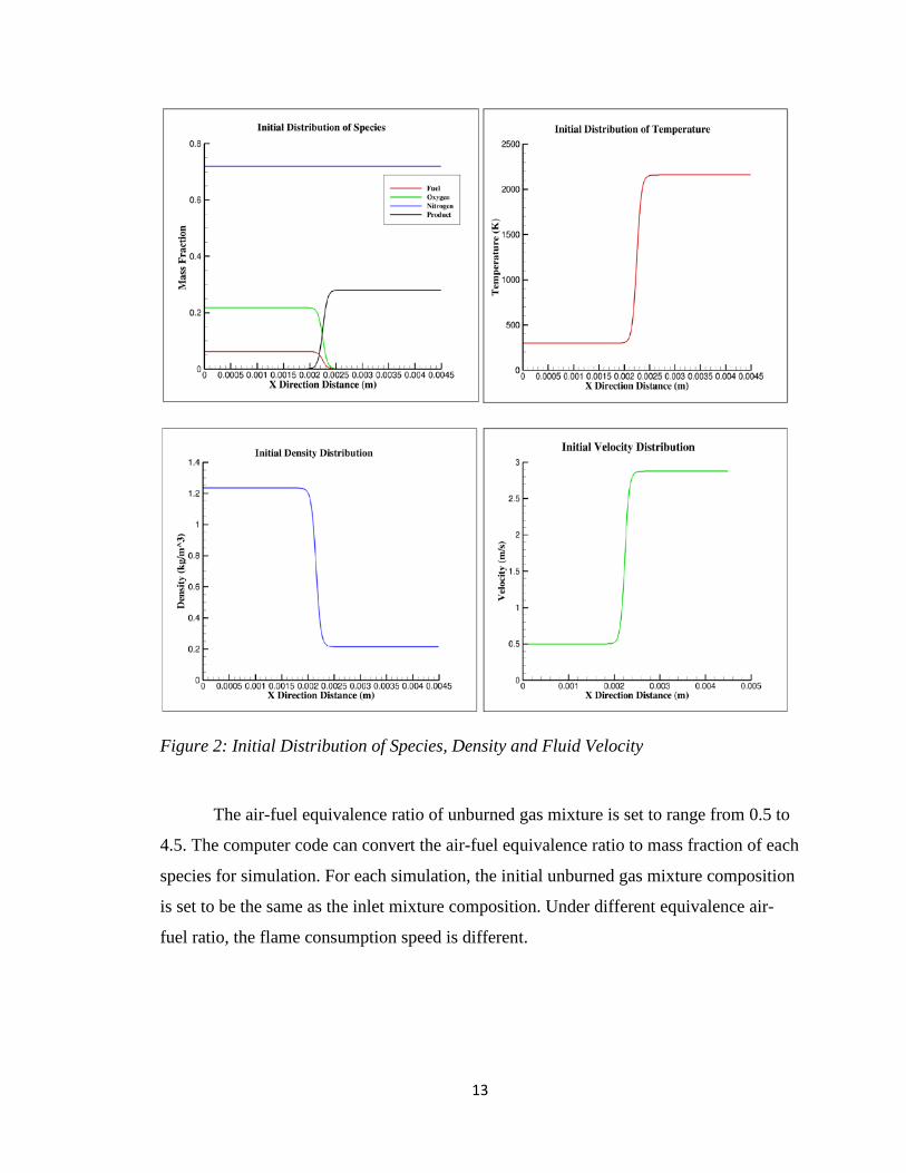
2.1.2 Distribution of Species, Temperature and Fluid Velocity The gas mixture components include fuel, oxygen, nitrogen and products. Both

the distribution of species and initial flow velocity along the simulation domain follow

the hyperbolic tangent function. This initialization enables flame to start propagating

from the middle of simulation domain towards unburned region with unburned gas

mixture continuously injected from inlet.

13

Figure 2: Initial Distribution of Species, Density and Fluid Velocity

The air-fuel equivalence ratio of unburned gas mixture is set to range from 0.5 to

4.5. The computer code can convert the air-fuel equivalence ratio to mass fraction of each

species for simulation. For each simulation, the initial unburned gas mixture composition

is set to be the same as the inlet mixture composition. Under different equivalence air-

fuel ratio, the flame consumption speed is different.

14

2.2 Initialization of Combustion Model 2.2.1 Chemical Reaction Formula The fuel that is used is n-heptane whose chemical formula is C7H16. The chemical

reaction formula can be written as:

C7H16+11(O2+3.76N2) →7CO2+8H2O+41.36N2 (1)

The molecular mass as well as the chemical reaction formula coefficient are put into the

code for initialization. Those information combined with air-fuel equivalence are utilized

to calculate the density and mass fraction of each species.

2.2.2 Single Step Chemical Reaction Parameters In order to generate the combustion and flame propagation, the chemistry model

needs to be utilized. Recent research has proved the importance of detail chemical

kinetics in modeling the structure of flames. On the other hand, there is a continuing need

for simple and reliable chemistry model to generate experimental flame propagation. [5]

To be specific, the simulation of flame propagation in 2D and 3D geometry needs to

consume a large amount of computational capacity. The use of detailed kinetic chemistry

model would further the computational cost. In this case, the single step chemistry

reaction model is utilized. The simplified combustion model sets the temperature,

activation energy, concentration of fuel and oxidizer as the factors that influence the

reaction rate. The equation is defined as:

Kov=ATnexp(-Ea/RT)[Fuel]a[Oxidizer]b [5] (2)

where

𝐾𝐾𝑜𝑜𝑜𝑜 = 𝑅𝑅𝑅𝑅𝑅𝑅𝑅𝑅𝑅𝑅𝑅𝑅𝑅𝑅 𝑅𝑅𝑅𝑅𝑅𝑅𝑅𝑅 (mole/s)

𝐸𝐸𝑎𝑎 = 𝐴𝐴𝑅𝑅𝑅𝑅𝑅𝑅𝐴𝐴𝑅𝑅𝑅𝑅𝑅𝑅𝑅𝑅𝑅𝑅 𝐸𝐸𝑅𝑅𝑅𝑅𝐸𝐸𝐸𝐸𝐸𝐸 (𝐽𝐽)

R=Ideal Gas Constant (8.314 𝐽𝐽 ∗ 𝑚𝑚𝑅𝑅𝑚𝑚𝑅𝑅−1𝐾𝐾−1)

T=Temperature (K)

a, b= Rate Parameters

[Fuel], [Oxidizer] = Concentration (mole/𝑚𝑚3)

𝐴𝐴𝐴𝐴𝑛𝑛 = 𝑃𝑃𝐸𝐸𝑅𝑅 𝐸𝐸𝐸𝐸𝐸𝐸𝑅𝑅𝑅𝑅𝑅𝑅𝑅𝑅𝑅𝑅𝑅𝑅𝑅𝑅𝑚𝑚 𝐹𝐹𝑅𝑅𝑅𝑅𝑅𝑅𝑅𝑅𝐸𝐸 ( 𝑚𝑚3/(𝑚𝑚𝑅𝑅𝑚𝑚𝑅𝑅. 𝑆𝑆)

15

Refer to equation 2, several parameters need to be set for each specific fuel. Since this

simulation use n-heptane as fuel, according to recent research, the parameters are set as

following.

Pre-exponential Factor ATn

(m3/(mole.S) )

5.1 × 1011

Activation Energy Ea (J) 125520

Rate Parameter a 0.25

Rate Parameter b 1.5

Flammability Limits 0.5 to 4.5

Table 1: Single Step Reaction Rate Parameters [5]

Aside, the change of temperature is based on the reaction rate, heat of combustion of fuel

and specific heat of gas mixture. Heat of combustion can be calculated by taking the

difference of enthalpy of formation of reactants and products. For heptane, the heat of

combustion is 4.58× 106 J/mole under complete combustion condition. Furthermore,

based on detail chemistry simulation, the temperature ranges from 298 K to 2200 K for

equivalence air-fuel ratio being set to be 1. The temperature of flame front is around

1500K.

Figure 3: Adiabatic Flame Temperature (Stoichiometric n-heptane Air-Fuel Equivalence Ratio) and Specific Heat Distribution

16

In this case, for simplification, the value of specific heat is set to be 1380 J/ (kg.K), which

is corresponding to 1500 K temperature. Given specific heat of gas mixture and heat of

combustion, the temperature change can be calculate as following:

∆𝐴𝐴 = 𝑄𝑄𝐾𝐾𝑜𝑜𝑜𝑜𝐶𝐶𝑝𝑝𝜌𝜌

(3)

where

𝛻𝛻𝐴𝐴 = 𝐶𝐶ℎ𝑅𝑅𝑅𝑅𝐸𝐸𝑅𝑅 𝑅𝑅𝑜𝑜 𝑅𝑅𝑅𝑅𝑚𝑚𝐸𝐸𝑅𝑅𝐸𝐸𝑅𝑅𝑅𝑅𝑡𝑡𝐸𝐸𝑅𝑅 �𝐾𝐾𝑠𝑠�

𝑄𝑄 = 𝐻𝐻𝑅𝑅𝑅𝑅𝑅𝑅 𝑅𝑅𝑜𝑜 𝐶𝐶𝑅𝑅𝑚𝑚𝐶𝐶𝑡𝑡𝑠𝑠𝑅𝑅𝑅𝑅𝑅𝑅𝑅𝑅 (𝐽𝐽/𝑚𝑚𝑅𝑅𝑚𝑚𝑅𝑅)

Based on the governing equation, the change of temperature along the flame

propagation can be evaluated as:

∆𝐴𝐴 = 𝑄𝑄×𝐾𝐾𝑜𝑜𝑜𝑜𝐶𝐶𝑝𝑝×𝜌𝜌

(4)

where

𝑄𝑄 = 𝐻𝐻𝑅𝑅𝑅𝑅𝑅𝑅 𝑅𝑅𝑜𝑜 𝐶𝐶𝑅𝑅𝑚𝑚𝐶𝐶𝑡𝑡𝑠𝑠𝑅𝑅𝑅𝑅𝑅𝑅𝑅𝑅 (𝐽𝐽/𝑘𝑘𝐸𝐸)

𝐶𝐶𝑝𝑝 = 𝑆𝑆𝐸𝐸𝑅𝑅𝑅𝑅𝑅𝑅𝑜𝑜𝑅𝑅𝑅𝑅 ℎ𝑅𝑅𝑅𝑅𝑅𝑅 𝑅𝑅𝑜𝑜 𝑚𝑚𝑅𝑅𝐸𝐸𝑅𝑅𝑡𝑡𝐸𝐸𝑅𝑅 𝐸𝐸𝑅𝑅𝑠𝑠 (𝐽𝐽

𝑘𝑘𝐸𝐸 × 𝐾𝐾)

𝜌𝜌 = 𝐷𝐷𝑅𝑅𝑅𝑅𝑠𝑠𝑅𝑅𝑅𝑅𝐸𝐸 𝑅𝑅𝑜𝑜 𝑚𝑚𝑅𝑅𝐸𝐸𝑅𝑅𝑡𝑡𝐸𝐸𝑅𝑅 𝐸𝐸𝑅𝑅𝑠𝑠 �𝑘𝑘𝐸𝐸𝑚𝑚3�

In return, the temperature change would affect the reaction rate. Basically, the

chemical reaction would release heat, which increase the temperature. The increase of

temperature would intensify the chemical reaction. Both temperature and reaction rate

will reach a steady states after the flame is fully developed. Aside, the consumption of

fuel and oxidizer can be calculated as:

𝑆𝑆𝑅𝑅 = 𝑛𝑛𝑛𝑛∗𝑊𝑊∗𝐾𝐾𝑜𝑜𝑜𝑜𝜌𝜌

(5)

where

17

𝑆𝑆𝑅𝑅 =

𝐶𝐶𝑅𝑅𝑅𝑅𝑠𝑠𝑡𝑡𝑚𝑚𝐸𝐸𝑅𝑅𝑅𝑅𝑅𝑅𝑅𝑅 𝐸𝐸𝑅𝑅𝑅𝑅𝑅𝑅 𝑅𝑅𝑜𝑜 𝑜𝑜𝑡𝑡𝑅𝑅𝑚𝑚 𝑅𝑅𝑅𝑅𝑎𝑎 𝑅𝑅𝐸𝐸𝑅𝑅𝑎𝑎𝑅𝑅𝑜𝑜𝑅𝑅𝐸𝐸,𝑃𝑃𝐸𝐸𝑅𝑅𝑎𝑎𝑡𝑡𝑅𝑅𝑅𝑅𝑅𝑅𝐸𝐸 𝐸𝐸𝑅𝑅𝑅𝑅𝑅𝑅 𝑅𝑅𝑜𝑜 𝐸𝐸𝐸𝐸𝑅𝑅𝑎𝑎𝑡𝑡𝑅𝑅𝑅𝑅 (1𝑠𝑠)

𝑅𝑅𝑡𝑡 = 𝐶𝐶ℎ𝑅𝑅𝑚𝑚𝑅𝑅𝑅𝑅𝑅𝑅𝑚𝑚 𝑜𝑜𝑅𝑅𝐸𝐸𝑚𝑚𝑡𝑡𝑚𝑚𝑅𝑅 𝑅𝑅𝑅𝑅𝑅𝑅𝑜𝑜𝑜𝑜𝑅𝑅𝑅𝑅𝑅𝑅𝑅𝑅𝑅𝑅𝑅𝑅

𝑊𝑊 = 𝑀𝑀𝑅𝑅𝑚𝑚𝑅𝑅𝑅𝑅𝑡𝑡𝑚𝑚𝑅𝑅𝐸𝐸 𝑊𝑊𝑅𝑅𝑅𝑅𝐸𝐸ℎ𝑅𝑅 (𝑘𝑘𝐸𝐸𝑚𝑚𝑅𝑅𝑚𝑚𝑅𝑅

)

According to the temperature change and consumption and producing rate

equations, we can map the distribution of temperature, fuel, oxidizer and product along

the flame propagation range.

Figure 4: Distribution of Temperature, Product, Fuel and Oxidizer.

18

Chapter 3: Flame Propagation, Heat Transfer, and Quenching

3.1 Flame Propagation There are several parameters being used to monitor the flame propagation. One of

them is the flame consumption speed. It is evaluated by integrating along the

simulation domain:

𝑆𝑆𝐿𝐿 = − 1𝜌𝜌𝑌𝑌𝑓𝑓

∫ 𝐾𝐾𝑜𝑜𝑜𝑜 𝑎𝑎𝐸𝐸 +∞−∞ (6)

where

𝑌𝑌𝑓𝑓 = 𝑀𝑀𝑅𝑅𝑠𝑠𝑠𝑠 𝐹𝐹𝐸𝐸𝑅𝑅𝑅𝑅𝑅𝑅𝑅𝑅𝑅𝑅𝑅𝑅 𝑅𝑅𝑜𝑜 𝐹𝐹𝑡𝑡𝑅𝑅𝑚𝑚 in Unburned Mixture

𝜌𝜌 = 𝐷𝐷𝑅𝑅𝑅𝑅𝑠𝑠𝑅𝑅𝑅𝑅𝐸𝐸 𝑅𝑅𝑜𝑜 𝑈𝑈𝑅𝑅𝐶𝐶𝑡𝑡𝐸𝐸𝑅𝑅𝑅𝑅𝑎𝑎 𝑀𝑀𝑅𝑅𝐸𝐸𝑅𝑅𝑡𝑡𝐸𝐸𝑅𝑅 𝑘𝑘𝐸𝐸/𝑚𝑚3

𝑆𝑆𝐿𝐿 = 𝐶𝐶𝑅𝑅𝑅𝑅𝑠𝑠𝑡𝑡𝑚𝑚𝐸𝐸𝑅𝑅𝑅𝑅𝑅𝑅𝑅𝑅 𝑆𝑆𝐸𝐸𝑅𝑅𝑅𝑅𝑎𝑎 (𝑚𝑚𝑠𝑠

)

Consumption speed of flame highly depends on chemical reaction rate, initial

pressure, and unburned gas temperature. Chemical reaction rate is determined by the

Equivalent air-fuel ratio, temperature and fuel type. In this case, under the same initial

conditions, the adjustment of Equivalent air-fuel ratio and fuel type would change the

consumption speed.

The Consumption speed is a reference parameter to set the inlet flow velocity. At

the steady state, if the inlet flow velocity is smaller than the consumption speed, flame

front will move towards to inlet. If the inlet flow velocity is larger than consumption

speed, the flame front will be pushed to the end of simulation domain. In order to have a

stable and fully developed flame, the inlet flow velocity should be equal to the flame

consumption speed.

19

Another important factor is the flame thickness. There are serval definition of

flame thickness. One definition that is used in this research is based on the temperature

change.

Figure 5: Definition of Flame Thickness

Flame thickness is mainly determined by the diffusivity of the gas mixture and chemical

reaction rate. Diffusivity changes with temperature, which is shown as following. Aside,

the correlation of viscosity has the same form as diffusivity.

𝐷𝐷 = 𝐷𝐷0(𝑇𝑇𝑇𝑇0

)0.75 (7)

where

𝐷𝐷 = 𝐷𝐷𝑅𝑅𝑜𝑜𝑜𝑜𝑡𝑡𝑠𝑠𝑅𝑅𝐴𝐴𝑅𝑅𝑅𝑅𝐸𝐸 𝑅𝑅𝑅𝑅 𝐴𝐴𝑅𝑅𝑚𝑚𝐸𝐸𝑅𝑅𝐸𝐸𝑅𝑅𝑅𝑅𝑡𝑡𝐸𝐸𝑅𝑅 𝐴𝐴 �𝑚𝑚2

𝑠𝑠�

𝐷𝐷0 = 𝐷𝐷𝑅𝑅𝑜𝑜𝑜𝑜𝑡𝑡𝑠𝑠𝑅𝑅𝐴𝐴𝑅𝑅𝑅𝑅𝐸𝐸 𝑅𝑅𝑅𝑅 𝐴𝐴0 = 298𝐾𝐾 �𝑚𝑚2

𝑠𝑠�

The diffusivity is in direct relation to the flame thickness. To be specific, the larger the

diffusivity, the quicker the unburned gas mixture is feed into the flame. Under the same

chemical reaction rate, this amount of fuel needs to be consumed over a longer distance.

The chemical reaction rate is in indirect relation to flame thickness. Under the same

diffusivity, the larger the chemical reaction rate, the quicker the fuel gets burned. In this

case, the fuel would be burned in a shorter distance.

20

The last parameter to evaluate the flame propagation is the maximum flame

temperature. The flame temperature is determined by the chemical reaction rate, specific

heat of gas mixture and heat of combustion. The simulation temperature is often used to

compare with the experimental results for validation.

3.2 Walls Heat Transfer The presence of conduction enables the energy to transfer from the flame across

walls. In order to account for the heat transfer, each grid point except for the walls has an

energy balance governing equation based on the first law of thermodynamics. In terms of

differential equation, the energy balance equation can be rewritten as:

' ( )p T

DTC TDt

ρ ω λ= +∇ ∇ (9)

where

'

1

N

T k kk

hω ω=

= −∑

kh =Enthalpy of species k

The wall heat transfer flux is evaluated as

wTqn

λ ∂= −∂

(10)

where

n = wall normal direction.

Additionally, the temperature of walls is set to be constant. Given this boundary

condition and energy balance equation, the heat transfer occurs between the fluid and the

walls.

3.3 Quenching When the flame propagates through a small diameter tube whose diameter ranges

1mm to 10 mm, the heat transfer of the walls can cause the quenching of flame. The

quenching distance is refer to the minimum diameter of tube for flame propagation

21

through. In order to derive the equation. There are two criteria that are ignition criteria

and quenching criteria. The ignition criteria mentions that the ignition will happen only if

enough heat is transferred to the unburned gas that is as thick as steady laminar flame

thickness to adiabatic flame temperature. The quenching criteria defines that the

quenching will occur when the heat from chemical reaction of the flame front is less than

the heat transfer out of the system.

Figure 6: Illustration of Flame Quenching Model [8]

The energy balance equation is listed as following:

recQ V = ,cond totQ (10)

where

V = Volume of Flame Front Region

recQ = 𝐻𝐻𝑅𝑅𝑅𝑅𝑅𝑅 𝑅𝑅𝑚𝑚𝑅𝑅𝑅𝑅𝑠𝑠𝑅𝑅 𝐹𝐹𝐸𝐸𝑅𝑅𝑚𝑚 𝐶𝐶ℎ𝑅𝑅𝑚𝑚𝑅𝑅𝑅𝑅𝑅𝑅𝑚𝑚 𝑅𝑅𝑅𝑅𝑅𝑅𝑅𝑅𝑅𝑅𝑅𝑅𝑅𝑅𝑅𝑅

,cond totQ = 𝐻𝐻𝑅𝑅𝑅𝑅𝑅𝑅 𝐿𝐿𝑅𝑅𝑠𝑠𝑠𝑠 𝑜𝑜𝐸𝐸𝑅𝑅𝑚𝑚 𝐶𝐶𝑅𝑅𝑅𝑅𝑎𝑎𝑡𝑡𝑅𝑅𝑅𝑅𝑅𝑅𝑅𝑅𝑅𝑅

The volumetric heat release rate recQ can be calculated as following:

recQ = − '''Fm ∆ℎ𝑐𝑐 (11)

where

22

'''Fm = 𝑉𝑉𝑅𝑅𝑚𝑚𝑡𝑡𝑚𝑚𝑅𝑅𝑅𝑅𝐸𝐸𝑅𝑅𝑅𝑅 𝑀𝑀𝑅𝑅𝑠𝑠𝑠𝑠 𝑃𝑃𝐸𝐸𝑅𝑅𝑎𝑎𝑅𝑅𝑡𝑡𝑅𝑅𝑅𝑅𝑅𝑅𝑅𝑅 𝑅𝑅𝑅𝑅𝑅𝑅𝑅𝑅 𝑅𝑅𝑜𝑜 𝐹𝐹𝑡𝑡𝑅𝑅𝑚𝑚 (𝑘𝑘𝐸𝐸/𝑠𝑠 − 𝑚𝑚3)

∆ℎ𝑐𝑐 = 𝐶𝐶ℎ𝑅𝑅𝑅𝑅𝐸𝐸𝑅𝑅 𝑅𝑅𝑜𝑜 𝐸𝐸𝑅𝑅𝑅𝑅ℎ𝑅𝑅𝑚𝑚𝐸𝐸𝐸𝐸 (𝐽𝐽𝐾𝐾𝐸𝐸

)

The heat conduction across the walls can be calculated as following:

wcond T

dTQ kAdx

= − (12)

where

A = 2 Lδ (Area between the Flame Front and Walls (m2))

K = Heat Transfer Coefficient (W/ (m2K))

Tw = Wall Temperature (K)

Based on above relation, the energy balance Equation can be derived as following:

(− '''Fm ∆ℎ𝑐𝑐)( dLδ ) = k ( 2 Lδ )

/b wT Td b− (13)

'''1 b

u

T

F Fb u T

m m dTT T

=− ∫

(14)

where

'''Fm = Average Volumetric Mass Production Rate of Fuel (kg/s-m3)

Tb = Burned Region Temperature (K)

b = Parameter that is greater than 2

/

b wT Td b− = Temperature Gradient from Centerline to Walls

Based on above relations, the quenching distance d can be correlated with flame

thicknessδ .

23

d bδ= (15)

The theoretical result indicates that the quenching distance is greater than flame

thickness for various fuels.

24

Chapter 4: Simulation of Flame Propagation 4.1 Flame Propagates in One dimensional Open Space The one dimensional open space simulation is used for validating the overall

simulation model by comparing the results from single step simulation with experimental

data.

4.1.1 Initialization of Model For open space simulation, there is no walls defined around the flame. The grid

points are used to mesh x direction only. The left set of domain is set to be inlet and the

right side is set to be outlet. Fluid is free to flow in either direction in open space.

X Distance

(m) Y Distance

(m)

X Direction

Mesh

Y Direction

Mesh

Thermal Dynamic

Pressure (Pa)

Initial Unburned Gas

Temperature (K)

0.0045 0.0020 750 1 101325 298

Table 2: Initial and Boundary Conditions of One Dimensional Open Space Flame Propagation

4.1.2 Model Validation After flame stabilizes, the temperature profile is shown as following. There is no

temperature gradient along vertical direction since the walls are absent. The simulation

domain is divided by the flame front to the unburned and burned region.

25

Figure 7: Distribution of Fluid Velocity and Temperature (Unit:m/s,K, Stoichiometric n-heptane Air-Fuel Equivalence Ratio, TUnburned =298K,PInitial=1atm,Simulation Time: 5.7595E-03 s)

For comparison, the consumption speed and adiabatic flame temperature are extracted

from single step chemistry simulation to compare with the experimental data [7].

Figure 8: Graph of Validation of Flame Consumption Speed and Adiabatic Temperature

Based on the above graph, the single step chemistry model correctly predicts the flame

consumption speed when air-fuel equivalence ratio ranges from 0.5 to 1. On the other

side, the result shows a serious errors for rich mixtures. The adiabatic flame temperature

of single step chemistry is 2159.3 K and the adiabatic temperature of experiment is

0

0.1

0.2

0.3

0.4

0.5

0.6

0.000 1.000 2.000 3.000 4.000 5.000

Flam

e C

onsu

mpt

ion

Spee

d (m

/s)

Air-Fuel Equivalence Ratio

Flame Consumption Speed Vs. Air-Fuel Equivalence Ratio Experimen

tal Data

SingleStepChemistry

2159.32250.0

0

500

1000

1500

2000

2500

Adi

abat

ic F

lam

e Te

mpe

ratu

re (K

)

Adiabatic Temperature (Stoichimetric Air-Fuel Ratio) Single Step

Chemistry

Experimental Data

26

2250.0 K. Therefore, we can predict the simulation results of following model for lean

mixtures are more accurate.

4.2 Flame Propagation in a Two Dimensional Channel with Adiabatic Walls Under the presence of adiabatic walls at the bottom and top, fluid flow is

predicted to be affected by the walls. There is no heat flux across the walls. The velocity

of gas is zero as gas propagating normal to the walls. The left side is set to be inlet and

right side is set to be outlet. The gas is free to flow in x and y direction at the open

boundary condition. The boundary condition is shown in the following table.

X Distance

(m) Y Distance

(m)

X Direction

Mesh

Y Direction

Mesh

Thermal Dynamic

Pressure (Pa)


Temperature (K)

0.0045 0.0020 750 300 101325 298

Table 3: Initial and Boundary Conditions of Two Dimensions Adiabatic Walls Flame Propagation

There are two tests cases associated this. One case has the fuel injection from the inlet. The other case does not have the fuel injection. These two cases are used to investigate how the presence of fuel injection affect distribution of flame properties.

4.3 Flame Propagation in a Two Dimensional Channel with Conductive Walls (Tube Quenching Model)

Tube quenching simulation is also conducted in the two Dimension domain. The

initial condition and boundary condition are set as following, which is the same as

adiabatic case except for the temperature of walls are set to be a constant value Tw. Also,

there is no fuel injection from the inlet. The flame propagates from the middle of

simulation domain towards the inlet. In reality, the temperature of walls varies within 10

K when quenching happens [6]. Therefore, it is a reasonable approximation of walls

temperature.

X Distance

(m) Y Distance

(m)

X Direction

Mesh

Y Direction

Mesh

Thermal Pressure

(Pa)


Temperature (K)

0.0045 0.0020 750 300 101325 298

Table 4: Initial and Boundary Conditions of Two Dimensions Conductive Walls Flame

Propagation

27

For each air-fuel equivalence ratio and unburned gas temperature, the quenching

distance can be found by shrinking the diameter of tube till the flame stop propagating.

However, this method is time-consuming especially for fine mesh and large size channel.

In this case, the approximation method is utilized. Based on the flame propagation in one

dimensional open space, the relationship between chemical reaction and temperature can

be extracted. According to figure

Figure 9: Relationship between the Chemical Reaction Rate and Temperature

9, the maximum chemical reaction rate is 124758 mole/ (m3.s). We assume that the temperature that corresponds to 5% of the maximum chemical reaction rate is the temperature for flame quenching. The quenching temperature is 1052.0K. Based on this, we can find the distance from walls to this temperature region. The quenching distance is twice of this distance. The test is aim to research the relationship between quenching distance and air-fuel equivalence ration and unburned gas temperature.

28

Chapter 5: Test Cases and Result Analysis 5.1 Flame Propagation in a Two Dimensional Channel with Adiabatic Walls The presence of adiabatic walls around flame would affect the flame propagation.

Figure 10: Fluid Velocity and Temperature Profiles in a Two Dimensional Channel with Adiabatic Walls and Fuel Injection (Unit:m/s, K, Stoichiometric n-heptane Air-Fuel Equivalence Ratio, Tunburned=298K,PInitial=1atm,Simulation Time:1.80050E-03 s )

The fluid velocity boundary layer is formed near the walls due to viscosity, which stretch

the temperature profile. Due to the area of flame front increases caused by the stretching,

the consumption speed increases significantly, which is equal to 1.03m/s for

Stoichimetric n − hepatne air− fuel equivalence ratio.

With fuel injection from the inlet, the low temperature unburned gas push the high

temperature burned gas towards to the outlet and form a V shape. Without fuel injection,

the depth of V shape is smaller compared with the case with fuel injection. The V shape

is only due to the velocity boundary layer that forms along vertical direction

29

Figure 11: Fluid Velocity Profiles and Temperature in a Two Dimensional Channel with

Adiabatic Walls and no Fuel Injection (Unit:m/s,K, Stoichiometric n-heptane Air-Fuel

Equivalence Ratio, Tunburned=298K, PInitial=1atm,Simulation Time:2.00000E-3)

5.2 Flame Propagation in a Two Dimensional Channel with Conductive Walls (Tube Quenching Model) The presence of conductive walls surrounding the flame would significantly affect

the temperature profile along vertical axis. The fluid velocity boundary layer forms near

the walls due to viscosity. The thermal boundary layer also forms near the walls due to

heat transfer. As the flame further develops, the high temperature region will shrink. At

the steady state, the area of high temperature region and the temperature gradient will

become constant.

Figure 12: Fluid Velocity and Temperature Profiles in a Two Dimensional Channel with Conductive Walls (Unit:m/s,K, Stoichiometric n-heptane Air-Fuel Equivalence Ratio, Tunburned=298K, Twall=298K, PInitial=1atm,Simulation Time:1.70000E-3s )

30

Figure 13: Relationship between Quenching Distance & Flame Thickness and Air-Fuel Equivalence Ratio (Tunburned =298K, Twall=298K, PInitial=1atm)

The magnitude of quenching distance ranges from 1.10 mm to 1.37 mm. The

minimum quenching distance occurs when the air-fuel equivalence ration is equal to 1.

The quenching distance increases as the air-fuel equivalence ratio deviates from 1. The

flame thickness ranges from 0.77 mm to 1.47 mm, which is smaller than the quenching

distance under every air-fuel equivalence ratio except for 0.5. The flame thickness has the

same trend as quenching distance. This result also meets equation 15 that indicates that

the quenching distance is predicted lager than the flame thickness.

0.00E+00

2.00E-01

4.00E-01

6.00E-01

8.00E-01

1.00E+00

1.20E+00

1.40E+00

1.60E+00

0 1 2 3 4 5Que

nchi

ng D

ista

nce

& F

lam

e Th

ickn

ess

(mm

)

Air-Fuel Equivalence Ratio

Flame Thickness & Quenching Distance Vs. Air-Fuel Equivalence Ratio Quenching

DistanceFlame Thickness

31

Chapter 6: Summary & Conclusions 6.1 Flame Propagation in a Two Dimensional Channel with Adiabatic Walls Based on the simulation result, the presence of adiabatic walls makes the fluid

velocity boundary layer form near the walls. Due to the non-uniform velocity profile, the

area of flame front increases, which increases the flame consumption speed. The

temperature profile is also stretched to be a V shape because the high speed and low

temperature unburned gas near the centerline blows the high temperature burned gas

backward.

When there is no fuel injection into the combustion channel, the temperature and

velocity profiles are similar to those for the case with fuel injection. Since there is no low

temperature unburned gas, the depth of the V shape of both the temperature and velocity

profiles are smaller than the case with fuel injection.

6.2 Flame Propagation in a Two Dimensional Channel with Conductive Walls (Tube Quenching Model) Based on the relationship between the quenching distance and air-fuel

equivalence ratio, the minimum quenching distance occurs when air-fuel equivalence

ration is equal to 1. The quenching distance will increase as the air-fuel equivalence ratio

deviates from 1. The flame thickness is smaller than the quenching distance and has the

same trend as the quenching distance. This result also meets the theoretical relationship

between the quenching distance and flame thickness.

32

Chapter 7: Recommendation and Future Work This research focuses on using n-heptane as the fuel. In the future, the fuel type

can be changed. Furthermore, this research only studies the flame propagation in a two

dimensional domain. Future research will explore three dimensional cases, which is more

practical.

In addition to the tube quenching, head on quenching is another important flame

wall interaction model. It is typically used for studying the auto ignition inside the

engine, which is also called engine knock. In the future, the head on quenching model can

be built based on the current model. The inlet will be replaced by a conductive wall with

a constant temperature. The flame can propagate towards the wall perpendicularly.

During the propagation, the quenching will happen as the flame approaches the wall. In

order to study the quenching, the chemical reaction rate of the flame front will be

extracted. We can predict that the chemical reaction rate will decrease as the flame front

approaches the wall. During this study, we can change the fuel type, initial pressure,

unburned gas temperature, wall temperature, size and geometry of the simulation domain

and air-fuel equivalence ratio. Based on those factors, we can map how each factor

affects the head-on-quenching. The head on quenching research can be done in both two

and three dimensional domains.

33

Appendix

34

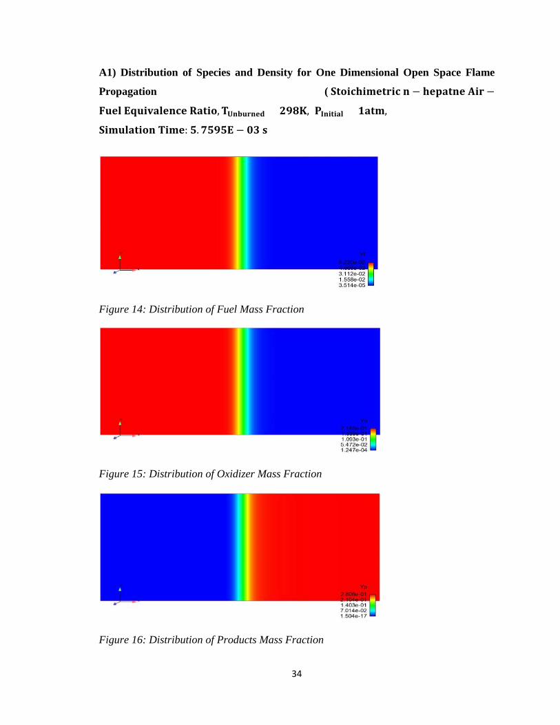
A1) Distribution of Species and Density for One Dimensional Open Space Flame

Propagation ( 𝐒𝐒𝐒𝐒𝐒𝐒𝐒𝐒𝐒𝐒𝐒𝐒𝐒𝐒𝐒𝐒𝐒𝐒𝐒𝐒𝐒𝐒𝐒𝐒𝐒𝐒 𝐧𝐧 − 𝐒𝐒𝐒𝐒𝐡𝐡𝐡𝐡𝐒𝐒𝐧𝐧𝐒𝐒 𝐀𝐀𝐒𝐒𝐒𝐒 −

𝐅𝐅𝐅𝐅𝐒𝐒𝐅𝐅 𝐄𝐄𝐄𝐄𝐅𝐅𝐒𝐒𝐄𝐄𝐡𝐡𝐅𝐅𝐒𝐒𝐧𝐧𝐒𝐒𝐒𝐒 𝐑𝐑𝐡𝐡𝐒𝐒𝐒𝐒𝐒𝐒,𝐓𝐓𝐔𝐔𝐧𝐧𝐔𝐔𝐅𝐅𝐒𝐒𝐧𝐧𝐒𝐒𝐔𝐔 = 𝟐𝟐𝟐𝟐𝟐𝟐𝟐𝟐, 𝐏𝐏𝐈𝐈𝐧𝐧𝐒𝐒𝐒𝐒𝐒𝐒𝐡𝐡𝐅𝐅 = 𝟏𝟏𝐡𝐡𝐒𝐒𝐒𝐒,

𝐒𝐒𝐒𝐒𝐒𝐒𝐅𝐅𝐅𝐅𝐡𝐡𝐒𝐒𝐒𝐒𝐒𝐒𝐧𝐧 𝐓𝐓𝐒𝐒𝐒𝐒𝐒𝐒: 𝟓𝟓.𝟕𝟕𝟓𝟓𝟐𝟐𝟓𝟓𝐄𝐄 − 𝟎𝟎𝟎𝟎 𝐬𝐬 )

Figure 14: Distribution of Fuel Mass Fraction

Figure 15: Distribution of Oxidizer Mass Fraction

Figure 16: Distribution of Products Mass Fraction

35

Figure 17: Distribution of Density (Unit:m3/s)

36

A2) Distribution of Species and Density for Two Dimensional Channel with Adiabatic

Walls Flame Propagation with Fuel Injection ( 𝐒𝐒𝐒𝐒𝐒𝐒𝐒𝐒𝐒𝐒𝐒𝐒𝐒𝐒𝐒𝐒𝐒𝐒𝐒𝐒𝐒𝐒𝐒𝐒𝐒𝐒 𝐧𝐧 − 𝐒𝐒𝐒𝐒𝐡𝐡𝐡𝐡𝐒𝐒𝐧𝐧𝐒𝐒 𝐀𝐀𝐒𝐒𝐒𝐒 −

𝐅𝐅𝐅𝐅𝐒𝐒𝐅𝐅 𝐄𝐄𝐄𝐄𝐅𝐅𝐒𝐒𝐄𝐄𝐡𝐡𝐅𝐅𝐒𝐒𝐧𝐧𝐒𝐒𝐒𝐒 𝐑𝐑𝐡𝐡𝐒𝐒𝐒𝐒𝐒𝐒,𝑻𝑻𝑼𝑼𝑼𝑼𝑼𝑼𝑼𝑼𝑼𝑼𝑼𝑼𝑼𝑼𝑼𝑼 = 𝟐𝟐,𝑷𝑷𝑰𝑰𝑼𝑼𝑰𝑰𝑰𝑰𝑰𝑰𝑰𝑰𝑰𝑰 =

𝟏𝟏𝑰𝑰𝑰𝑰𝟏𝟏, 𝐒𝐒𝐒𝐒𝐒𝐒𝐅𝐅𝐅𝐅𝐡𝐡𝐒𝐒𝐒𝐒𝐒𝐒𝐧𝐧 𝐓𝐓𝐒𝐒𝐒𝐒𝐒𝐒:𝟏𝟏.𝟐𝟐𝟎𝟎𝟎𝟎𝟓𝟓𝟎𝟎𝐄𝐄 − 𝟎𝟎𝟎𝟎 𝐬𝐬)




37


38

A3) Distribution of Species and Density for Two Dimensional Channel with Adiabatic

Walls Flame Propagation without Fuel Injection ( 𝐒𝐒𝐒𝐒𝐒𝐒𝐒𝐒𝐒𝐒𝐒𝐒𝐒𝐒𝐒𝐒𝐒𝐒𝐒𝐒𝐒𝐒𝐒𝐒𝐒𝐒 𝐧𝐧 − 𝐒𝐒𝐒𝐒𝐡𝐡𝐡𝐡𝐒𝐒𝐧𝐧𝐒𝐒 𝐀𝐀𝐒𝐒𝐒𝐒 −

𝐅𝐅𝐅𝐅𝐒𝐒𝐅𝐅 𝐄𝐄𝐄𝐄𝐅𝐅𝐒𝐒𝐄𝐄𝐡𝐡𝐅𝐅𝐒𝐒𝐧𝐧𝐒𝐒𝐒𝐒 𝐑𝐑𝐡𝐡𝐒𝐒𝐒𝐒𝐒𝐒,𝑻𝑻𝑼𝑼𝑼𝑼𝑼𝑼𝑼𝑼𝑼𝑼𝑼𝑼𝑼𝑼𝑼𝑼 = 𝟐𝟐,𝑷𝑷𝑰𝑰𝑼𝑼𝑰𝑰𝑰𝑰𝑰𝑰𝑰𝑰𝑰𝑰 =

𝟏𝟏𝑰𝑰𝑰𝑰𝟏𝟏, 𝐒𝐒𝐒𝐒𝐒𝐒𝐅𝐅𝐅𝐅𝐡𝐡𝐒𝐒𝐒𝐒𝐒𝐒𝐧𝐧 𝐓𝐓𝐒𝐒𝐒𝐒𝐒𝐒:𝟐𝟐.𝟎𝟎𝟎𝟎𝟎𝟎𝟎𝟎𝟎𝟎𝐄𝐄 − 𝟎𝟎𝟎𝟎 𝐬𝐬)



39

Figure 24: Distribution of Product Mass Fraction


40

A4) Distribution of Species and Density for Two Dimension Conductive Walls

Flame Propagation ( 𝐒𝐒𝐒𝐒𝐒𝐒𝐒𝐒𝐒𝐒𝐒𝐒𝐒𝐒𝐒𝐒𝐒𝐒𝐒𝐒𝐒𝐒𝐒𝐒𝐒𝐒 𝐧𝐧 − 𝐒𝐒𝐒𝐒𝐡𝐡𝐡𝐡𝐒𝐒𝐧𝐧𝐒𝐒 𝐀𝐀𝐒𝐒𝐒𝐒 −

𝐅𝐅𝐅𝐅𝐒𝐒𝐅𝐅 𝐄𝐄𝐄𝐄𝐅𝐅𝐒𝐒𝐄𝐄𝐡𝐡𝐅𝐅𝐒𝐒𝐧𝐧𝐒𝐒𝐒𝐒 𝐑𝐑𝐡𝐡𝐒𝐒𝐒𝐒𝐒𝐒,𝑻𝑻𝑼𝑼𝑼𝑼𝑼𝑼𝑼𝑼𝑼𝑼𝑼𝑼𝑼𝑼𝑼𝑼 = 𝟐𝟐,𝐓𝐓𝐖𝐖𝐡𝐡𝐅𝐅𝐅𝐅𝐬𝐬 = 𝟐𝟐𝟐𝟐𝟐𝟐𝟐𝟐,𝑷𝑷𝑰𝑰𝑼𝑼𝑰𝑰𝑰𝑰𝑰𝑰𝑰𝑰𝑰𝑰 = 𝟏𝟏𝑰𝑰𝑰𝑰𝟏𝟏,

𝐒𝐒𝐒𝐒𝐒𝐒𝐅𝐅𝐅𝐅𝐡𝐡𝐒𝐒𝐒𝐒𝐒𝐒𝐧𝐧 𝐓𝐓𝐒𝐒𝐒𝐒𝐒𝐒: 𝟐𝟐.𝟎𝟎𝟎𝟎𝟎𝟎𝟎𝟎𝟎𝟎𝟎𝟎 − 𝟎𝟎𝟎𝟎 𝒔𝒔)




41


42

References [1] T. J. Poinsot, D. C. Haworth, and G. Bruneaux, “Direct Simulation and Modeling of Flame-Wall Interaction for Premixed Turbulent Combustion.” Combustion and Flame 95: 118-132 (1993).

[2] A. Dreizler, B. Bohm, “Advanced laser diagnostics for an improved understanding of premixed flame-wall interactions.” Proceeding of the Combustion Institute 35 (2015) 37-64.

[3] H. Yu, Z. Chen, “End-gas autoignition and detonation development in a closed chamber, Combustion and Flame (2015)”. http://dx.doi.org/10.1016/j.combustflame.2015.08.018

[4] O. Desjardins, G. Blanquart, G. Balarac, H. Pitsch, High order conservation finite difference scheme for variable density low mach number turbulent flows, J. Comput. Phys. 227 (2008) 7125 - 7159

[5] C. K. Westbrook & F. L. Dryer (1981) “Simplified Reaction Mechanism for the Oxidation of Hydrocarbon Fuels in Flames.” Combustion Science and Technology, 27: 1-2, 31-43

[6] A. A. Adamczyk and G. A. Lavoie, “A Numerical Study of Laminar Flame Wall Quenching.” Combustion and Flame 40: 81-99 (1981).

[7] R. Zhao, H. Liu, X. J. Zhong, Z. J. Wang, Z. Q. Jin, Y. M. Chen, J. R. Qiu, “The Ignition Delay, Laminar Flame Speed and Adiabatic Temperature Characteristics of n-Pentane, n-Hexane and n-Heptane Under O2/CO2 Atmosphere”. Cleaner Combustion and Sustainable World (2013). DOI 10.1007/978-3-642-30445-3_10.

[8] Stephen R. Turns, “An Introduction to Combustion: Concepts and Applications” 3rd Edition, McGraw-Hill Education (2011)

Documents

Undergraduate Honors Thesis By Shuhan Li Undergraduate