UNCLASSIFIED

AD NUMBER

LIMITATION CHANGESTO:

FROM:

AUTHORITY

THIS PAGE IS UNCLASSIFIED

AD913801

Approved for public release; distribution isunlimited.

Distribution authorized to U.S. Gov't. agenciesonly; Test and Evaluation; JUN 1973. Otherrequests shall be referred to Office of NavalResearch, Arlington, VA 22203.

ONR ltr 2 Mar 1979

THIS REPORT HAS BEEN KUftlTCT

AKD Cf, EARED 90H PUBL«C REÜiÄSC

UNDER DOD DIRECTIVE 52C0.20 AND

HO RESTRICTIONS ARE IMPOSED UPON

ITS USE AND DISCLOSURE.

DISTRIBUTION STATEMENT A

APPROVED FOR PUBLIC RELEASE;

DISTRID^TION UN'LIKITED.

a o

DUtrl^tlon lifted ^ U.S. UoV%. »f™»^ **«

PSR REPORT 506

June 1973

ELECTROtttGNETIC COMMUNICATION IN THE EARTH'S CRUST

F.C. Field M. Dore

/— e

as ti ioo >n

Sponsored by *^\ f\ r\

ADVANCED RESEARCH PROJECTS AGENCY ARPA Order No. 2270

The views and conclusions contained In this document are those of the authors and should not be Interpreted as necessarily representing the official policies, either expressed or Implied, of the Advanced Research Projects Agency of the U.S. Government.

PACIFIC-SIERRA RESEARCH CORP. MM

.

pnpiwiu'«' « ' -' imaiiiiiii.iiiiiiiMVPIil11.«."'«-11 ^«F^^WVPapRiiliWMV^Pn i..jiii«iL|iipip^nr«^OT ■*,ii^iiinu4. ■« «i ii

... f, v»t. aRencIe9 Anlrl

PSR REPORT 306

June 1973

ELECTROMAGNETIC COMMUNICATION IN THE EARTH'S CRUST

E.G. Field H. Done

Sponsored by

ADVANCED RESEARCH PROJECTS AGENCY ARPA Order No. 2270

The viewe end conclusions contained in this docuaent ere those of the authors end should not be interpreted es necessarily representing the official policies, either ezpreeeed or implied, of the Advanced Research Projecte Av-ercy of the U.S. Govemeent.

r^ PACIFIC-8IKRRA RKBBARCH CORP. MB ■—Mi mm.

'■— - - - -■

ARPA Order No.:

Program Code No.:

Name of Contractor:

Effective Date oi Contract:

Contract Expiration Date:

Amount of Contract:

Contract Number:

Principal Investigator:

Scientific Officer:

I'hone Number:

Short Title of Work:

2770

3F10

Pacific-Sierra Researcii Corp,

72 November 01

t DtH fmbor ) 1

■%8,010.00

N00014-73-C-0189

Edward C Field

Jolin G. lleacock

(213) 828-7461

Litliospheric Communication

This research was supported by the Advanced Research Projects Agency

M! Snnn??a^,Dr' °! DefenSe and WaS ^"^ored by ONR under Contract No. N000U-73-C-0189.

^■^^■PP"""«'"'' —-. iunaumn" jmt.iiym^r- ■i.^"^"' •v.ni ... 11 ii

•ili-

PREFACE

Pacific-Sierra is performing a study of possible military applica-

tions for ar. electromagnetic waveguide in the lithosphere. This report

presents the results of the first phase of that study; viz., a determina-

tion of the data rates and transmission ranges that, based on currently

used models of the lithosphere, might be achievable with reasonable power

expenditure and antenna burial depths. These results form the scientific

basis for the second phase of the study, which is to determine those

missions for which use of a lithospheric communication link could be

feasible.

The motivation for this work stems from the integrated studies of

crustal properties that have been conducted for a number of years by

the Earth Physics Program of the Office of Naval Research. This effort

was brought into focus by a Symposium, jointly sponsored by ONR and CIRES,

held in July 1970. The proceedings of this symposium were published in

AGU Monograph //14, The Structure and Fhysiaal Properties of the Earth's

Crust (1971). Subsequently, two workshops, funded by ARPA and organized

by ONR, were held at the Colorado School of Mines, in February 1972, to

define an experimental program to ascertain the existence tf the litho-

spheric waveguide.

m^KK^^^^m

PRßCüD'tfC PAGE BLANK-NOT FILLED

-v-

SUMMARY AND CONCLUSIONS

This report presents results of an analysis of the capabilities

that might he achieved with a lithospheric communication system. The

analysis uses several available models of continental lithospheric

conductivity as inputs to calculations of transmission characteristics

and possible communication system parameters. Because of prevailing

uncertainties, significant differences exist among the various models;

and a wide range of future system capabilities is found to lie within

the realm of possibility. Full-wave modal solutions that take full

account of vertical conductivity gradients are used to calculate attenua-

tion rates, field-strength depth-profiles, and transfer functions

relating the noise fields at depth to those measured at the surface.

Also, estimated values of required system power are given as a function

of data rate, transmission range, and receiver burial depth. Carrier

frequencies from 100 Hz to 100 kHz are considered. IL could well prove

worthwhile, however, to extend the analysis to frequencies outside of

the ELF/VLF/LF bands treated herein.

For all models used, the calculated attenuation rates are con-

siderably larger than for above-ground transmission, which depends on

propagation in the earth-ionosphere waveguide. In spite of this fact,

reasonably large transmission ranges might be possible in the lithosphere

because the atmospheric noise fields at depth are very small, having

suffered heavy attenuation in propagating downward from the earth's

surface.

The major factor affecting system feasibility is whether water-

saturated microcracks exist in all major rock types at depths greater

MiMMa^MMIMiitakHua

PFUiC

- I - --

iDTtC PAGE BLANK-NOT FUMED

Mtf^MÜMMi

**m ■— Jii .iiWI .i,^-!!»^^^! - ■jfH447miV"«nPNH' •IVHI>VUIIRU ii iimwp"

-vl-

than, say, 5-to-8 km. If such microcracks exist (as assumed in one

-5 -6 . model), and minimum conductivities in the crust exceed 10 - 10 mhos/m,

then the calculations show clearly that a practical communication system

is not feasible. For this case, the attenuation rates are so high that

only very short transmission ranges could be achieved, even if large

amounts of power were expended. Field experiments will be needed to

determine with certainty whether saturated microcracks are, in fact,

present at the depths of Interest. However, valid reasons exist for

optimism that fluids (or fluid films) should not be an important factor

at depths greater than several kilometers, and that conductivity profiles

(at depth) based on laboratory data for dry rocks more closely approxi-

ma te actual conditions. Further, recent laboratory data indicate that

-8 the conductivity of dry rock in the crust could be much lower (10 to

10 mhos/m) than previously believed (10 mhos/m). It is, of course,

difficult to relate data obtained from laboratory samples to conductivities

of rock in situ. Nonetheless, calculations using conceptual profiles

based on the assumption of dry basement rock yield results that are

quite encouraging. For example, for data rates of a few tens ol bits-

per-second and power expenditures of I-to-10 megawatts, transmission

ranges of from about 1000 to many thousands of kilometers (depending

on the profile used) appear to be a possibility.

The calculations show clearly that much larger transmission ranges

can be achieved in the LF band (30-100 kHz) than at the lower fre-

quencies considered. This effect is due mainly to the heavy attenua-

tion suffered by downward propagating atmospheric noise at the higher

frequencies. The calculations also show that the maximum transmission

j -- ■ - —

MHWMHMü^ MMMHH

*~-~-m^mm

■Vll

ranges are somewhat sensitive to the details of the model profiles,

''or example, for two profiles exhibiting the same minimum conductivity,

the transmission range (for a specified power, etc.) can vary by a

factor of two depending on the conductivity depth-gradients, and the

precise jocation of any sharp transition layers that might exist.

The depth to which a rei.eiver must be burisd to achievp satisfac-

tory performance is a particularly important parameter, siritc borehole

d'Uling costs could be a large fraction of the total system cost.

The transmission ranges given above apply when the receiving antenna

is 'ccated near the "center" of the waveguide—assumed to be about

ten kilometers deep for the conductivity profiles used in this

report. For profiles tepresentative of regions stripped ul highly

conducti/e sedimentary layers, the calculations show that receiver

depths as shallow as 3 or 4 km could be used at only a lS-to-20 percent

penalty in transmission range. One implication of this fact .'s that —

previous negative results notwithstanding--a meaningful propagation

experiment could be carried out with relatively shallow boreholes,

provided that the region was carefully selected. Frequencies of

several tens of kilohertz would be preferable, and care should be

taken to Insure a reasonable transmitter efficiency. Of course,

deeper boreb-les would be needed in regions having thick, highly

conducting overburdens.

Another type of propagation experiment, not involving a trans-

mitter, has appeal for ascertaining the existence, or non-existence,

of a lithospheric waveguide. There are regions of the sea floor where

little or no sedimentation exists, and where energy propagating in a

1 '■••'■"

-vili-

lithospheric waveguide could conceivably approach the ocean's bottom

from below. In deep water, the preferred propagation path (to the

bottom) for atmospheric noise would be via a lithospheric duct, rather

than downward from the ocean's surface, due to the opacity of sea water

to all frequencies higher than. say. a few Hertz. Consider an experi-

ment where atmospheric noise was measured as a function of the depth

(in the water) of the receiving antenna. For shallow receiver depths,

this noise would decrease as the receiver depth was Increased. If.

however, the noise (e.g.. Schumann resonances) was then found to

increase as the receiver ap.:oached or contacted the bottom, consider-

able credence would be given to the presumed existence of a crustal

waveguide.

..., .. ...^——,^—^—„^.»j,J._^i^J^_^, mtm

*m^mi*^m*mmmm mmmmm**w v* « wmmn^mm^viy*****^'—

-lx-

CONTENTS

Ill PREFACE

SUMMARY AND CONCLUSIONS

Section . i I. INTRODUCTION

II. MODELS OF ELECTRICAL CONDUCTIVITY AND NOISE IN THE ^ LITHOSPHERE 3 Conductivity Depth-Protlies 13 Atmospheric and Thermal Noise

Ill. MATHEMATICAL FORMULATION '.','..'.. 16 Modal SolutIons 22 Atmospheric and Thermal Noise • Achievable Data Rates and Transmission Range

IV. NUMERICAL RESULTS AND DISCUSSION • • •'' ^ Attenuation Rates ••• ,„ Signal and Noise Field-Strength Profiles •••••••••••;•••■ 1Z Dependence of Slgnal-to-Nolse Ratio on Receiver Depth ... 47 Transmission Ranges and Power Requirements

64 REFERENCES

^ ■_.. ^^ .^——^^

-"""-'""" " —■ - WW^^^FIP^-— T"-»^

-1-

I. INTRODUCTION

More than a decade has passed since the existence of an electro-

magnetic waveguide in the earth's crust was first postulated (e.g.,

Wait, 1954; Wheeler, 1961). The assumption was that conductive, wet

surface layers and conductive, hot mantle layers enclose a resistive

zone of dry basement rocks. As originally conceived, the resistive

zone occupied depths between roughly 10 and 30 km. Interest in ascer-

taining the existence, or non-existence, of this lithospheric waveguide

stemmed from its potential use as a communication channel. In the

intervening years enthusiasm about the prospect of a crustal waveguide

waned, partially because of the apparently negative outcome ot propaga-

tion experiments carried out between ]9b2 and 1966 C-:'-', :.v.').

In retrospect, it appears that, due to experimental limitations, the

data thus obtained could not have either confirmed or denied the exis-

tence of a waveguide in the lithosphere.

Little is known in detail about the precise nature of the materials

and physical properties of the earth's crust at depths where the resistive

basement rocks are presumed to exist. The available data base is by

no means complete, and additional field measurements are needed if firm

values are to be assigned to key parameters. However, reinterpretation

-7 . of available field data has indicated that (. onductivities of 10 mhos/in

or lower could exist. Moreover, recent laboratory experiments on the

conductivity of dry rock, and recent evidence based on minerologlcal

considerations, suggest cause for optimism that conductivities lower

-8 than previously believed might exist in the crust (e.g., ' 10 mhos/m).

Theoretical analyses show that the corresponding attenuation rates for

.-^^.^.„^ _ ..

—- ———

electromagnetic waves could be low enough to permit communication

over useful distances. For these reasons, there has been renewed

interest in determining the electrical properties of the lithosphere

and in assessing its potential utility as a communication channel.

Workshops have been held, and recommendations made that interdisci-

plinary field-measurement programs be undertaken {Keller, J9?Zi Hales,

'972).

This report presents results of an analysis of capabilities that

might be achieved with a lithospheric communication system. As might

be expected in view of prevailing uncertainties, a wide range of future

system capabilities is found to lie within the realm of possibility.

However, the results give guidance as to whether it is reasonable to

expect, on the basis of current knowledge, that a lithospheric wave-

guide would provide the basis for useful communication links.

The lithospheric conductivity models used in the calculations are

given and discussed in 3ec. II, as are models of atmospheric and thermal

noise. The mathematical methods used are described in Sec. Ill, and

numerical results, obtained from Pacific-Sierra's long-wave propagation

code are given in Sec. IV.

II. MODELS OF ELECTRICAL CONDUCTIVITY AND NOISE IN THE LITHOSPHERE

The electromagnetic transmission properties of the lithosphere

must be calculated in order to assess its utility as a communication

channel. This calculation requires a knowledge of the depth-profiles

of the electrical properties (primarily conductivity) of the earth's

crust and upper mantle, as well as a knowledge of the degree of lateral

homoegneity of these properties. In addition, tl noise, environment

at the receiver must be known to determine the relationships among

radiated power, transmission range, and data rate. Accordingly, the

models of conductivity and noise spectrum used as inputs to the calcula-

tions of Sees. Ill and IV are discussed below.

CONDUCTIVITY DEPTH-PROFILES

Considerable uncertainty exists as to the conductivity of the

earth at depths greater than several kilometers. This uncertainty is

due to practical difficulties encountered in using surface-based sound-

ing techniques to detect low conductivities at depth, and an absence

of sufficiently deep boreholes for direct measurements. However,

nominal models for conductivity depth-profiles in the lithc-phere

have been suggested by various geophysicists. As might be expected

in view of the prevailing uncertainties, significant differences exist

among currently available model profiles. This state of affairs is

unfortunate, since the results given in Sec. IV show that the trans-

mission properties of the lithosphere depend strongly on the minimum

value of conductivity in the crust, as well as on the depth-gradients

of the conductivity.

— ■■-■ ■ ■— -

-4-

It Is necessarily beyond the scope of this study to determine the

correcc depth-profile of conductivity In the llthosphere. Indeed, the

main goal of the Crustal Studies »orkshop (Hales, et at., 1972) was to

consider and suggest experimental procedures by which profiles could be

determined. The approach taken In this report Is to use currently

available conductivity oflles, which In our opinion are reasonable

In the context of present knowledge, as Inputs to our calculations.

This approach provides the most reliable estimates that can now be made

of the txpected performance of a llthospherlc communication system, and

also indicates the sensitivity of llthospherlc transmission properties

to variations in the profiles. Guidance Is thereby obtained as to

whether more extensive experimental determinations of llthospherlc

conductivities are likely to reveal the existence of a useful crustal

waveguide.

For a discussion of evidence for (and against) the existence of

an electromagnetic waveguide In the llthosphere, the reader Is referred

to AGU Monograph 14 (Heaaoak, ed., 1971) and Crustal Studies Workshop

Report (Hales, 1972). Briefly, the conductivity of rocks near the

earth's surface Is relatively high due to the presence of water In

pores and cracks. As the depth Is Increased, the contribution of pores

and cracks to the conductivity is diminished due to increasing pressure;

the conductivity will thereiore decrease with increasing depth. There

is, however, a competing effect; viz., the temperature increases by

some 10o-to-30oK for each additional kilometer of depth. Ultimately,

conductivity due to thermal-activated carriers in hot rock should be-

come dominant. The conductivity should then increase with increasing

-■——■A-- -—■ ■ - „____ ■- - - ■

-5-

4

depth. There is thus reason to expect a layer of relatively low

conductivity to exist between a surface layer (overburden) that is

highly conductive because it contains fluid and a sub-basement that

is highly conductive because it is hot. This poorly conducting layer,

if it exists, would comprise the lithospheric waveguide that is the

subject of this study. Geophysiclsts have given much attention to

ascertaining the minimum value of conductivity in the waveguide, since

this value strongly influences the transmission properties. Presently,

the value of minimum conductivity is uncertain by several orders of

magnitude.

For the purpose of making calculations, the so-called "step-

function" representation of the conductivity profile is the simplest.

Here, the lithosphere is assumed to form a uniform parallel-plate

waveguide, bounded on the top by a highly conducting overburden and on

the bottom by a highly conducting sub-basement. The region between

these two sharp boundaries contains rock of low conductivity. Spies

and Wait (1972) performed an extensive and useful parametric study of

the transmission properties of a parallel-plate model of the lithosphere.

Specifically, they calculated attenuation rates and excitation functions

as functions of wave frequency, waveguide width, wavegulc-e conductivity,

and boundary conductivity. Although the step-function representation

of the conductivity profile provides insight into th« dependence of the

transmission on several key parameters, we have chosen to use more

detailed profiles. This choice was made because 1) the signal attenua-

tion depends on the depth-gradients of the conductivity, which cannot

be included in a step-function profile; and 2) the depth to which

! . ,^i, Mmi

ÜMMtfli ■^HMMMMM

antennas must be burled tu provide adequate reception (or radiation)

cannot be calculated satisfactorily from a step-tunctlon model. To

ascertain the depth dependences of the signal and noise fields, finite

conductivity gradients must be included in the model.

A major source of uncertainty is the water content of rocks at

depths greater than a few kilometers. One view holds that microfractures

are not present in rocks at depths that have never been merhanically un-

loaded from lithostatic compressior.. Such rocks would be dry and have

a very low electrical conductivity. Another view is that water films

* in microcracks must be present at all depths in the crust (Bmee, 1971).

Hypothetical conductivity profiles that illustrate the implications of

the above two points of view have been prepared by levin (1971) and are

shown in Fig. 1. Each profile exhibits a "waveguide" at depths between

about 10 and 30 km. The conductivities at shallow depths are based upon

available, shallow geophysical measurements; those below about 30 km

are estimated from assumed temperature gradients in the rock. The profiles

shown in Fig. 1 differ only in the "waveguide" region between 10 and 30 km.

The segments labeled "wet" and "dry" are nominal representations based

upon early laboratory measurements of "wet" and "dry" rocks, respectively.

Under the hypothesis of "wet" rock, the minimum conductivity shown Is

about 10 mhos/m; and for dry rock, about 10 mhos/m. The profiles

in Fig. 1 are intended only to illustrate the range of uncertainty in

the expected minimum conductivity, and are nominal rather than detailed

Whether such saturated microcracks exist in all major rock types in situ is still undetermined. However, for several reasons, there appears to be increasing optimism that dry, low-conductivity zones can exist in the crust (see, e.g., Hales, 1972; p. 28).

MMMUWaiBiiidttUilfaMaMft - - ■ ~ •AMBMIMI ■-•-' ■ ----■" ^-- ■ ■- . kJ—

-7-

10

E

■£ 20 Q.

IMI | I I 1 [llll | I I 1 [Mill I I 1 [MM Mil [MM I I I T

0) Q

30

40 liui I

10 ,-3

I I ll ■ l l I l I l III! l I l I | llll 1 1 1 i

■4 .-.-5 ,„-6 lllll I I I L

10^ lO' 10

Conductivity, mhos/m

10 r7 10

Fig. I--Conductivity Profiles of the Crust According to Two Hypotheses (after Levin, 1972)

■MMMMMMMn

-— - - — ii

-8-

representations. Further, as discussed below, recent laboratory measure-

ments- not available when Levin's profiles were prepared—indicate that

the minimum conductivity could well be considerably less than 10 mhos/m.

Of the currently available conductivity profiles, the one based

on the most extensive measurements is probably that shown in Fig. 2

{Keller as reported by Gallrnkx and Haidle, 2972). Although uncertain

in several respects, this profile represents a compilation of a good

deal of geophysical and laboratory -data. The conductivities shown for

relatively shallow depths are based upon well-log data, taken in

Appalachia, that clearly indicate a decreasing conductivity down to at

least several kilometers. This decreasing trend in conductivity is

believed to be controlled by the rate at which fractures close due to

increasing overburden pressure. Below, say, 3-to-5 km, the decrease in

conductivity was extrapolated, in a manner consistent with available

field and laboratory data, to a minimum value referred from recent field

measurements.* Below about 10-to-12 km, the conductivity is assumed to

be dominated by high-temperature mineral conduction. The values shown

for depths below 10-to-12 km in Fig. 2 are based on laboratory measure-

ments of high-temperature rocks. The assumed temperature scale is shown

on the right-hand axis of Fig. 2, and corresponds to a nominal thermal

gradient of 160/km.

In addition to temperature, the conductivity at depth also depends

on mineralogy. Note that in Fig. 2 Keller has assumed a rapid transition

*For a discussion of the various methods of probing the electrical properties of the crust, and a discussion of the difficulty in obtaining and interpreting da»a on deep layers of low conductivity, see Keller

(1971).

- ■ - ■ —

-9-

N)|0 '3in\Oiadaia\ pa4DUJi4sg

n «n r\ o ^_ CO IT) r^ o o CN

CN CO en

oo es IT) 00 LO

CO

'O n —r I 1 1 1 1 1 "1 n

■

o o

- c o

o Q

en y | -

: ■'

-

o o a. o W

3

o

_L "a) 5 /

^ S\

'E 0

6 /

U -- 'O

4-

t- ,n .1

- s \ / > ( "

c ;■

- > f

\ - 0)

- / \ t - / \ c — / i — — 8 / : E 0' CM ^^- 0 / — O '\ — t^

-

o

a> en o 4) > < \

en o /

/

-

o -T £

• - CJ t- ^ 1 O i- i a <i)

_ i / —

>- a) "y

-f- t* 10

- 5, / _ >

i i u

C

- y - 'o t

i / 0 0

- /

- f < »

/ / "v . / *" ■♦- >

- / f i ~ — £!

> - / \ _ — TJ : / \ « ■<» +- ai

—

s> V

'o u •»- ■n O i a

- o • -«- \- Cl I

_ in

O a - I i

_ O E - , - CO Ö

U - v. • -

- - n u.

~ 1 | I 1 1 1 1 'o o CN ■* o 00 O CN ■t ■o "

UJ>j 'i\\d3Q

mmm —^ -r-. — ■ - -

-10-

in conductivity at about 14 km. The existence of such a transition is

inferred from seismic data and certain electromagnetic field measurenents.

The lA-km depth at which the transition is assumed to occur is, of course,

nominal, and represents an average value for the United States. In some

regions, assumed transition-layer depths as large as 20-to-25 km are

consistent winh the available data (Keller, 197?). Another characteristic

of the Keller profile is that the conductivity at the earth's surface

-4 is taken to be about 10 mhos/m—a very low value. The use of a higher

-2 -3 surface conductivity (say, 10 to 10 mhos/m) would not change the con-

clusions of this report significantly, since the transmission properties

of the waveguide depend mainly on the properties of the crust at depths

below 1 or 2 km.

Recent laboratory measurements of the conductivity of dry rock

reported by Houslcy (197S) suggest that the minimum conductivity of the

crust might be considerably less than illustrated in Figs. 1 and 2.

He arguos that most previous laboratory data tend to give a misleading

picture of lithospheric conductivity at depths greater than, say, 10 km.

Rocks in situ should have much lower conductivity than rocks that have

been exposed to the atmosphere and that have had microcracks closed by

the application of high pressures in the laboratory. In the latter

case, thin films of interstitial fluid remain and raise the conductivity

by a considerable amount. In addition, Housley has found that the

partial pressure of oxygen in the atmosphere surrounding the sample

must be miiintained at a level corresponding to that in the crystal

at the temperature and pressure for the depth being simulated. The

data thus obtained indicate conductivities orders of magnitude less

.- - ■ MWMl

-11-

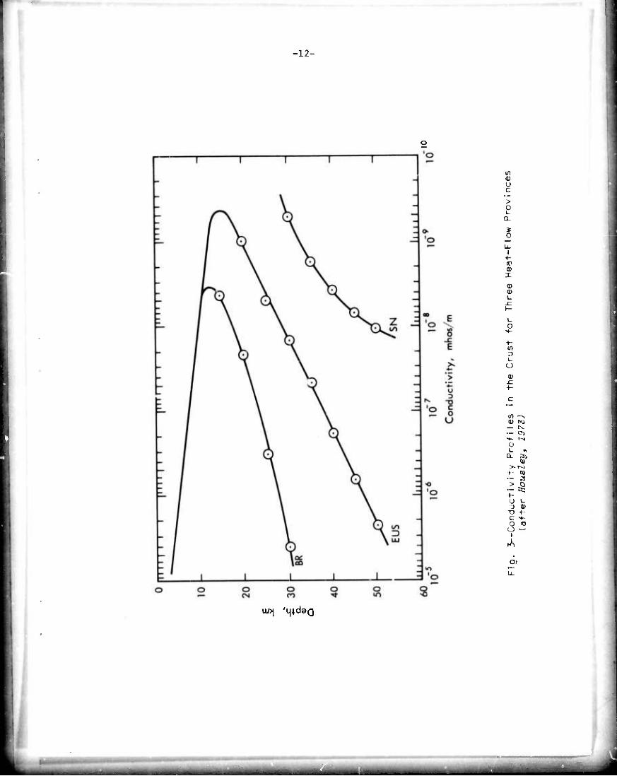
than previously measured for dry rocks in the laboratory. If one uses

these new conductivity data, and follows the same reasoning (see above)

that led to the profile shown in Fig. 2, the resultant profiles are as

shown in Fig. 3. These profiles are identical to Keller's (Fig. 2) for

depths less than about 10 km, since the same data and assumptions are

-8 used. At greater depths, however, much lower conductivities (<10 mhos/m)

are indicated, due to the new laboratory data described above. The

three profiles shown correspond to geotherms in three different heat-

flow provinces,* as reported by Blaakwell (1971). The thermal gradients

used were BR (-'240/km), EUS (~140/km), and SN (-v^/km) as compared

with the 160/km used for the Keller profile (Fig. 2).

It must be emphasized that the Fig. 3 profiles (or any others)

are by no means definitive, and much experimental work remains (some

of which is now underway) before a satisfactory understanding of the

conductivity of in situ rocks can be attained. Great uncertainty is

involved in using laboratory data to infer the conductivity of the

crust. Further, the data reported by Housley (1973) were for only a

single sample (olivine); but lithologies are not constant in nature.

However, these data do give encouragement that the minimum conductivity

of the crust might be lower than previously believed.

Clearly, the above discussion indicates selecting a single "best"

profiiP for making calculations would be impossible. Indeed, Fig. 3

alone shows the large variations that would occur among different

provinces. The Levin profile (Fig. 1) exhibits rather abrupt changes

in conductivity at depths of about 2 km and 7 km. The Keller profile

'BR (Basin and Range), EUS (Eastern, US), SN (Sierra Nevada).

HMMVHM

-12-

01

u L

> I a i 0

IC 0) .1

s I-

L O

U U

(0 —i

0) ^J — r^ ■— o> •♦ i-i 0 l- •»

u. 3, i

>KI^

+- CO .— a > o .— a: h U L.

> o " ♦ L *♦-

o in 15

Ol

UJ>| ,L|4da(]

'

■WM

mm—mm

■ - ■ -

■13-

(Fig. 2) exhibits a near-dlscontln'lty at around 14 km; whereas the

Housley profiles (Fig. 3) are quite smooth at all depths. Field

measurements are needed to determine which of the differences between

these (and other) profiles are artificial, and which correctly account

for real differences among various regions of the earth's crust. It

would not be practical, or very meaningful, to undertake detailed trans-

mission calculations for all available conceptual profiles. In Sec. IV,

rather complete computational results are given for the Keller and

Housley BR profiles; and sample results for other profiles, to indicate

important trends. When more accurate conductivity measurements become

available, the methodology developed here can be applied tn obtain

more reliable estimates of the transmission properties.

ATMOSPHERIC AND THERMAL NOISE

The noise environment at a buried receiver consists of thermal

noise, which depends upon the temperature distribution in the crust, and

atmospheric noise.- which propagates downward from the earth's surface.

We use the temperature profile given in Fig. 2 to compute thermal noise.

As discussed in Sec. Ill, reasonable variations from this profile change

the thermal-noise power density at the receiver by an insignificant

amount.

Extensive data for atmospheric noise at the earth's surface are

available fo various seasons and geograptilc locations. We use data

As shown in Sec. IV, the transmission properties of the litho- sphere depend strongly on whether abrupt transitions in the conductivity profile are present. In fact, some of the calculations given below are for the Housley BR profile, modified to have a sharp transition at a

depth of 25 km.

-14-

complled by Maxüell (1967). His rms nolse-denslty spectra for summer

and four representative locations are shown in Fig. 4. Maxwell's data

indicate that these rms atmospheric noise values are exceeded 10-to-20

percent of the time. Thus, a system designed on the basis of the rms

atmospheric noise will achieve, or exceed, performance specifications

80-to-90 percent of the time; i.e., it will have an 80-to-90 percent

time availability. If 99-percent time availability is required, then

the system should be designed on the basis of atmospheric-noise spectral

densities about 10 dB larger than those shown in Fig. 4. At the earth's

surface, the electric fields associated with atmospheric noise in the

ELF/VLF/LF bands are nearly vertical; whereas the magnetic fields are

nearly horizontal. The noise-field components at depth must be computed

for each conductivity profile from the surface-noise data. The details

of this calculation are given in Sec. III.

-

. .._-.■■ ^- ^—. ,____ *mm - - — -^-^-^

■' —■

MÜfc.

-15-

yy/y i 04 3AHD|aj 9p 'PH 'X4!su3p pjaij D^außouj |04UOZ!JOH

g § § § 8 T T T

T

yy/A [ 04 3A!4D|aj gp /P3 ,X4!Suap p|a!j 3!J43a|a |D3!4JaA

1

I. ■0) 4 T)

-t- u a) a

(/>

'.0

0) I 1

I a' in

o 2 c

O) H

- . M

-16-

III. MATHEMATICAL FORMULATION

In view of the inherent uncertainty in the conductivity depth-

profiles given in Sec. II, the choice of computational method requires

discussion. It is temping to argue that highly simplified analytic

techniques will suffice, since—regardless of the mathematical approach—

the final results will be no more accurate than the models used for inputs.

Although clearly correct, this argument should not be carried too far,

lest important general characteristics d the electromagnetic fields be

obscured. In particular, account must be taken of the depth gradients

of conductivity to gain insight into the depth dependence of the signal

and atmospheric noise fields. This insight is needed to determine the

dependence of system performance on antenna burial depths. Clearly, if

either transmitting or receiving antennas could be placed at relatively

shallow depths above the waveguide, system costs would be reduced signifi-

cantly. Conductivity gradients also strongly affect the lateral attenua-

tion in the waveguide. Since the wavelengths involved are not small

compared with vertical distances over which the electrical properties of

the lithosphere change substantially, eikonal methods are not applicable

and full-wave calculations are needed. To compute the lateral attenuation

and depth dependence of the fields, we have used a method that accounts

in detail for the vertical inhomogeniety of the lithospherlc conductivity.

We use simpler computational methods to account for lateral inhomogenietles

and to determine certain system performance parameters.

MODAL SOLUTIONS

We wish to determine the spatial dependence of the electromagnetic

fields propagating in a waveguide that is strongly inhomogeneous in the

I -"— - ....~~^.,^~^^^

-17-

vertical direction. The curvature of the earth will be neglected and

hcrlrontal stratification will be assumed (see Fig. 5). The method

of calculation Is a version of the waveguide mode analysis described

by Budden (1961). This method, often used in problems involving propa-

gation in the earth-ionosphere waveguide {e.g.. Field, 1970), has been

modified in this study for applicaiion to the llthosphere.

Although the best antenna configuration for use in a llthospheric

conmunication channel is Oft known, a vertically polarized E-field

antenna is a likely candidate. We thus consider plane TM waveg-tide

modes propagating in the x-direction. for which the electric field, E,

and the magnetic field can be written

E(x,Z) - [exEx(z) + ezEz(z)j •

i(ut-kn S x) o o (1)

Kajt-kn S x)

V;(x,z) - eyVy(z) e

In Eq. (I), V-yf^kK, where H is the usual magnetic intensity. U0 and

r are the electric and magnetic permittivities of free space, w - 2w« o

(where f is the wave frequency), t is tiae, and k - »/c (where c is the

vacuum speed of light). MKS units will be used. The refractive index,

n, is given by

2, x / N io(z) n (z) - e(z) - —- , ufo

(2)

where a is the depth-dependent conductivity and i is the relative electric

permittivity. The quantity no in Eq. (1) is the refractive index al the

_^^^^^^fc^^^^M1^^M ^-^^^^ tm^mmtam~m0^

tjpiKMRHh «1,1 ' ■ J"" ■ ■

18-

I ■ i

z

Earth's Surface

Free Space or

Sea Water

z =0

Fig. 5--Schematic Model of Lithospheric Waveguide

■ ■-■ - ii i^TiiMi»!—itiäi^ilMMüriiiiir»! ■ - ■ -

1 - • ' i «WH um im i ■ Mill III I IB II I^^V^H^HHHP^IHOTW ■JPUIH ipj. IIJI.

-19-

depth. z , of minimum conductivity In the llthosphere. So can be

Interpreted as the sine of the incidence angle at the depth zo. Incidence

angles at deptha other than z can be determined from the relation

S(z)n(z) - noS - constant. (3)

which follows from the assumed horizontal stratification and is essentially

Snell's law.

The relevant Maxwell equations are:

dl —^ + ikn S 1 dz o o J.

-lkVy ; CO

W ■ -ikn (z)E ;

dz x (5)

noSn O 0 V.. . n2(z) 'y

(6)

Rather than solving Eqs. (4) through (6) directly, we u^e the wave ad-

mittance, A, defined by

A 5 Vy/Ex . (7)

and the related quantity

W A-l A+l '

(8)

By combining Eqs. (4) through (8), it follows that

—^ iMu-mauiaiiMiMiM MnMMüMMIMMIiH

mm mmmmmmmmmmmm •'•' mmimm^m^^^' -—»•^™~—»»"—--—»^«.^P^IW™^»!

-20-

di 2

2Q2 -n S o o

V n2(z)

(W+l)' (9)

It is clear from Eq. (1) that the lateral attenuation in the waveguide

Is governed by the product n^. Since no Is specified once a llthospherlc

model and a wave frequency have been selected, only So must be calculated

to determine the attenuation. This calculation Involves the solution of

Eq. (9) subject to the appropriate boundary conditions, whence eigen-

values for S are found. A guided wave In the llfaosphere can produce o

only upgolng waves In the medium above the earth's surface, since this

medium Is assumed uniform with constant Index of refraction, n^ Thus,

Immediately above the earth's surface, the wave admittance Is given by

A(0+) [nJ-sW)]1'2 *

(10)

For propagation under the ocean, n1 Is the refractive Index of sea water,

and may be assumed Infinite for the frequencies to be considered. For

this case, A(0+) ■• - and, from Eq. (8), the boundary condition for W Is

simply

W(SoN.z-0) - I. (11a)

,th where S „ denotes the eigenvalue of 8 for the N mode. For the case

ON 0

where the medium above the earth's surface Is free space, n1 - 1; and,

using Eqs. (3), (8), and (10), the boundary condition on W becomes

W(SoN,z.O) -

2 2 I/2 1-<1-noSoN)

2 2 I/2 (lib)

________

^m^mimmmmmmmmmmmmm »^W<^i^PIWPW|(^W*P"^W^WW»W»llli. I

-21-

The conductivity profiles given In Sec. II, and values for e given

below, are sufficient to determine n2(z) for the various u^dels. Once

n2 is specified. Eqs. (9) and (11) comprise a closed set for W and S^.

These coupled equations are solved readily by straightforward Iteration.

Each iteration requires the numerical solution of Eq. (9). This solution

is started at a great depth, where a purely downgoing wave is assumed

fis an initial condition. In each solution, several starting depths and

integration step sizes are tried; and the process is truncated when

successive trials fall within a prescribed tolerance. The integration

is terminated at the earth's surface. For a profile such as that shown^

in Fig. 2. it is Inconvenient numerically to use downgoing waves at

great depths as an initial condition, since Integration across any zones

of rapid conductivity change (which, for the case shown in Fig. 2. would

be at 14 km) would be required on each iteration. For the profile in

Fig. 2. we found that the use of W(z-lA) - 1 as an Initial condition

provided good accuracy and considerable simplification. This initial

condltxon is equivalent to truncating the conductivity profile in a

perfect conductor at f—14 km.

Once the eigenvalue S^ is found and W (and hence A) is computed,

the attenuation rate for the Nth mode and the depth dependence of the

electromagnetic fields are easily obtained. The attenuation rate Is

given by

aN = 8.7 x 103kImSoN dB/km ;

(12)

and. by Integrating Maxwell's equations, it follows that

V (f) exp [-*/'*.• 4^] • (13)

^^^^^m^mn^jm^^^^^m^0^ . ^...-„...^~~i,^^.*j~*.i^*i~-*^ ^ ^^^^ÜJÜIi

»"•■ ■■ 1 ' ■" " ' ' ~ —— ■^^■■WW.il "1 i lii , Ulli-

-22-

E (z) z

n S -2-2- Vy(.). n2(z) y

(14)

and

Ex(z) V (z)/A(z), y

(15)

where V has been taken to equal unity at the "center" of the waveguide; y

i.e. at z-z . The time and x-dependence of the fields have been sup- ' * o

pressed in Eqs. (13) through (15).

ATMOSPHERIC AND THERMAL NOISE

To calculate achievable transmission ranges and data rates in the

lithosphere, it is necessary to know the atmospheric and thermal-noise

spectral density at the receiver depth. The atmospheric noise fields

at depth must be calculated from the available data, which are typically

in the form of vertical electric fields measured at the earth's surface

(see Fig. 4). The quantities that relate the noise fields at depth to

the surface noise fields will be called noise-transfer functions. For

uniform media, such as the ocean, the transfer functions can be calculated

easily in terms of plane waves and the well-known Fresnel reflection and

transmission coefficients. However, when the conductivity exhibits

significant depth-gradients (e.g., as in Figs. 1-3), the transfer functions

cannot be computed in closed form. Gallawa and midle (1972) accounted

for the vertical inhomogeniety of conductivity by representing the litho-

sphere by several uniform layers and computing the transfer function by

summing the absorptions suffered in each layer. However, even this

approach is not adequate for the problem at hand. It neglects both the

M^^^^^MM^bM^Ml^^M||M|^^ta

-23-

conversion loss suffered at the earth's surface and the fact that the

admittance "seen" by a downward propagating signal Involves an Integral

over all depths. Also, the total noise field at depth should not be

used, instead, the component of the noise field in the direction of the

antenna polarization is needed. Although the noise fields above the

earth's surface are nearly vertically polarized, the fields in the

highly refractive earth can be nearly horizontally polarized. And a

vertically-oriented, buried electric antenna (a likely configuration)

will be less sensitive to atmospheric noise than would a horizontally

orlenteo one. In fact, the strength and polarization of the subterranean

noise fields are related in a complicated fashion to the conductivity

profile and change continuously with depth. A full-wave numerical

calculation of these fields is thus needed. Fortunately, the procedures

developed to solve Eqs. (9) and (13) through (15) can be used essentially

without change.

The problem at hand is to relate the noise fields at depth to the

vertical atmospheric electric noise field. Eza(0). which is assumed known

at the earth's surface. Atmospheric noise typically propagates above the

earth's surface as a TM mode with an incidence angle larger than. say.

70°. Let the sine of this angle be denoted by 8^. The magnetic noise

field at the surface is then given by

V(0) " EZa(0)/Sa

(16)

The depth-dependent admittance seen by this signal can be computed by

.olving Eqs. (8) and (9). with zo - 0. whence So - Sa and no - 1. Note

that no iteration is needed since Sa is specified, and only a single

mm

■^■riMauiii iwn-ii-iii i 4,IJII»,IIBI jw^nii. ■■ .lu.ipv i

•24-

Integratlon of Eq. (9) is needed for each profile and wave frequency.

Once the admittance has beer thua determined, the transfer functions.

Y . are easily computed from Eqs. (13) through (15). The resulting

equations are:

V (z) - Y.E (0). va 1 za

(17a)

£Za

(z)-Y2EZa(0)'

(17b)

where

E (z) - Y_E (0). xa 3 za

(17c)

1 S. exp h/-'^]- (18.)

'2 ■ " -äTT Ti' n (z)

(18b)

and

Y3 - Y1/A(z) (18c)

Strictly speaking, the noise-transfer functions given above cannoc be

completely specified, since the incidence angle (and. hence. Sa). Is

never known precisely. However, these functions are very insensitive

to reasonable variations In Sa. For example, calculations for incidence

angles of 85° and 70° (a realistic range of values) yielded values for

Y that differed by less than 1 or 2 dB-an insignificant variation.

TIM results given In Sec. IV are computed for an assumed incidence angle

of 72° (S - 0.95). and should very accurately approximate the transfer

functions for all obliquely Incident noise fields.

^■PIPHPV1**"^" H^WWWWfK^pWWIP ll ^^mm^jmim 'm.-mi* mit 9im,r^mm^ ■ i

-25-

For propagation above the earth's surface and frequencies In the

LF band and below, atmospheric noise Is always much stronger than thennal

noise; and above-ground long-wave systems are atmospherically noise

limited. However, atmospheric noise Is attenuated In the earth's crust

and thus decreases w^th Increasing depth; and thermal noise becomes

greater with depth because of the higher temperatures. For certain

situations, thermal noise could be the limiting factor for a deeply

buried receiver. The thermal noise power density, NT, will be computed

from the simple relation

N - 1.38 x 10"23T watts/Hz , (19)

where T is the lithospheric te^erature at the receiver depth in decrees

Kelvin. T will be taken from the Keller model as shown in Fig. 2.

Equation (19) for NT is, of course, oversimplified. In a non-uniform

medium such as the lithosphere, the antenna receiver "sees" a continuum

of temperatures from the surrounding material. However, the error in-

curred by using Eq. (19) is quite small, as can be seen from the fact

that the temperature varies by less than a factor of 2 (less than 3 dB)

over the entire range of depths shown in Fig. 2. Further, other avail-

able lithosvheric models show temperatures that differ from those shown

in Fig. 2 by no iK>re than 20 percent. Gallaua and Haidle (1972) have

carried out detailed calculations of NT, taking proper account of antenna

directivity and integrating over the contribution from the surrounding

medium. As would be expected from the above discussion, their results

differ from those obtained from Eq. (19) by a few dB, at most. A few

dB are insignificant compared with other factors that Influence expected

system performance.

mpmnwmnwpm MV im i ^mimmirmm^f^i^mmmm^mmm^^^' i ai an m ■

26-

ArHTKVABLE DATA RATES_ANp TI^ANSMISSION RANGE

.. ,~r q reauired to achieve a data The signal power at the receiver, Sreq. reqiure

rate of R bits per second is given by

Sreu = [hf\tfK„ **" R (20)

req

uhere Eb is .he energy P« bit at th. receiver, and ».ff L. the e»ect4ve

(I.e.. the post-processing) noise-power density. We ssso.e l%l\ff\^ *■

*~ „f in-3 with simple DPSK modu- which is sufficient to achieve an error rate of 10 P

lation. Equation (20) thus becomes

S = 6N ,,- R req efl

(21)

For ahove-ground corniest ions, it is custody to include a signal

Mr8in to insure reliability even during adverse fluctuations in propaga-

tion conditions. Such a margin has not been included in Eq. (21). because

(unlikt the ionosphere) the lithospheric waveguide should be a very stable

communication channel.

,„ the following discussion, several Ideallratlons are n.de to render

the calcuUtlons of the received signal and noise trsctshle. T.ese spproxl-

Mtl„ns are necesssry hacause th. proble« of calculating the directivity

a„d effactlva ares of an sntanns Imbedded In a «edlu. that Is hoth con-

ductlv. ana inho^geneon. has never h.en solved. The directivity function

rf the receiving antenna Is needed hecause the signs! and .«spheric noise

artlve fro. very different dlr.ctlons-the signal propsgatlon helng «r.

or U.. lateral, whereas the atmospheric noise prop.gstes «.Inly vertically

in th. ..rth's crust. «. procd with th. c.lcul.tlon .. If th. r.c.lv-

mg .nt.nn. were bedded In . unlfor. ^dlu.. Although difficult to

..ftatu ^_^^^^^^ —

*^^^m*m*^mmni ^pmpp*)>a*"«^>p*MM(f||

■27-

Justify rigorously, this approach should give a reasonably good estimate

of the required power. For all of the lithospheric models except one

(Levin "wet" model. Fig. 1), the refractive index in the crust is fairly

uniform and has a small Imaginary part (implying a dielectric-like

medium) at depths where the conductivity is small and, hence, where a

receiver is apt to be placed. Moreover, although inaccurate in detail,

the expressions used do incorporate the important features of the

propagation and reception. For example, the expression used for antenna

directivity does correctly account for the fact that a vertical E-fleld

antenna is sensitive only to vertical electric fields, and thus mitigates

much of the atmospheric noise that is mainly horizontally polarized at

depth. The results thus should be adequate for this feasibility study.

For illustrative puvposes, we assume that the receiving antenna is

a short, vertical electric dipole. This configuration is a logical

choice, since it should fit easily into a narrow, vertical borehole,

and will be relatively insensitive to downward propagating atmospheric

noise. Note that detailed antenna design is beyond the scope of this

study, and future study could well demonstrate that some other configura-

tion is more attractive. However, it is unlikely that alterations in

receiver design would change the forthcoming conclusions regarding system

feasibility. For example, any realistic antenna must be fairly small

electrically because of the large wavelengths in the crust (> l-10km),

and all small antennas have about the same gain. Further, as is evident

from thp numerical results given in Sec. IV, system feasibility is

dominated by the attenuation of the signal and atmospheric noise In the

crust. Neither of these factors depend In any way on hardware design.

—- -^-. -. .. —>.—^fc- *^*M*~ä^—^—*—. ■ „_.

■28-

For the effective area of the receiving antenna, we use

A „(.) * 3{2 ^ aln e (-ters)2 . (22) eff ü) y e E (z)

o o

where the angle, 6, la measured relative to the vertical. The incident

intensities I and I . associated with the signal and atmospheric noise s a

density, respectively, are given by

I - 1/2 Ve /p Re(n(z)) E2(z) watts/m . o ^o

and

I = l/2Ve /u Re(n(z)) E2(z) watts/m -Hz , a ' o Ko a

(23)

(24)

where E is the total signal electric field and Ea is the noise-field

spectral density. Noting that E2 sln2e ■ E2, etc., it follows that

Signal Power ■ Re(n(z)) E,(z)

z

160 k2e(z) watts , (25)

and

u . ^4 Re(n(z)) E^fl(z) Atmospheric Noise m za Watts/Hz ;

Power Density 160 k e(z)

(26)

whereas the internal noise density is simply

N - 1.38 x 10"23 TF watts/Hz , (27)

where F is the receiver-noise figure. The effective noise density at

the receiver is thus

- - ^M J

■Wiwmiiipmiiiii f11 Iw.HWWlWi^U^IWiW ^WWWmwpiWP^™1^''IJ"-* ^'ma.mmiwmiamv^m

-29-

Re(n(z)) E_(z) za eff 2

160 kZe(z)G + .1.38 x 10~23TF watts/Hz , (28)

where G is the processing gain; i.e., the factor by which the effective P

atmospheric noise can be suppressed by using non-linear elements in the

receiver circuit.

By inserting Eqs. (25) and (28) into Eq. (21), we find the following

expression for the required vertical electric field at the receiver

(E2(z)) req

2 AP

Eza(z) . (160)(1.38 x 10"23)k2£ (z) __ 6R G + Re(n(z))

P

(2f)

The receiver is assumed to be at a depth, z. The final step for computing

required power is to relate the signal electric field, E (z), to the

transmitter power. This can be done approximately by noting that the

waveguide signal spreads nearly cylindrically from the source and also

suffers an exponential attenuation given by Eq. (1?). At a distance, d,

from the receiver, the signal-power density can be written in the form

n? exp[-10 Ja d/A.3] I ^ —-r H watts/ni. s 2iTd h ,,.

ef r

(30)

Only a single waveguide mode (the N ) has been used in Eq. (30), since

we are considering distances large enough that only the least attenuated

mode will contribute significantly. P is the total transmitter power,

and n is the transmitter efficiency; viz-, the fraction of the total

power that is radiated into the dominant (N ) waveguide mode. The

quantity h „ is defined by

••f-pmn . ,i .IMP i ■.■.laiiu in* wwn mi., iiii|.wj^mnniK,>u«i <• '—•'' ■ i mmm'^'^^m^m^mw ippr^invvi^^^nvinv^K^n^i^wcvi^Hiuiim' ^iiiniiifM

-

•30-

Vff " /

0 Re(n(z)) E (z)

dz' Re(n(zo)) E^(zo)

(31)

and represents the nominal width of the waveguide region that contains

«.t of the signal power. From Eqs. (17b). (23). and (29) through (31).

it follows that for a receiver located at the "center" (•-.,,) of the wave-

guide, the required transmitter power Is given by

67rRh f(:d ry eft

v o n req

Re(no)Y^(zo) E2za(0)

120TI G_

/4k2(:(zo) 1.38xl0'23T(zo)F

exp 10 aNd

4.3 (32)

For receiver depths other than zo. the required power can be estimated

from:

(P(z))~.„ " D(zHp0) req veq (33)

where the depth degradation factor. D. is given by

D(z) ^

E2(z)

Re(n (z))Y22(z)E2

a(0)

120it G

Re(r ̂o)>Y22^o)F-za(0)

120IT G_

(^)'- 38xl0"23T(z)F

k34)

t pp.). 38xl0"23T(zo)F

where z denotes the receiver depth, the transmitter depth being unspecified.

For systems limited by atmospheric noise, D simplifies to

__ «HMMMMÜMi

-31-

E2(Zo) Re(n(z)) Y^Cz)

D(z) ^ -r- 2 F/(z) Re(n(zo)) Y^)

(35)

For systems limited by thermal noise:

EZ(z ) eU) T(z)

D(z) ^-L-5 E2(z) t{z) T(fJ

(36)

The rat

in Sec. IV,

ionale used in selecting the various input parameters is discussed

. ***********

m— ""i.i im « • i ■■iip i ■

-32-

IV. NUMERICAL RESULTS AND DISCUSSION

Pacific-Sierra's long-wave propagation code is used to calculate

the attenuation rates, and the signal- and noise-wave functions, for

several of the model waveguides shown in Figs. 1 through 3. The results

of these calculations are given in this section. Detailed results are

also given for the required power as a function of data rate, trans-

mission range, and receiver burial depth. In all cases, the relative

electric permittivity, E, is assumed to have a constant value of ten.

ATTENUATION RATES

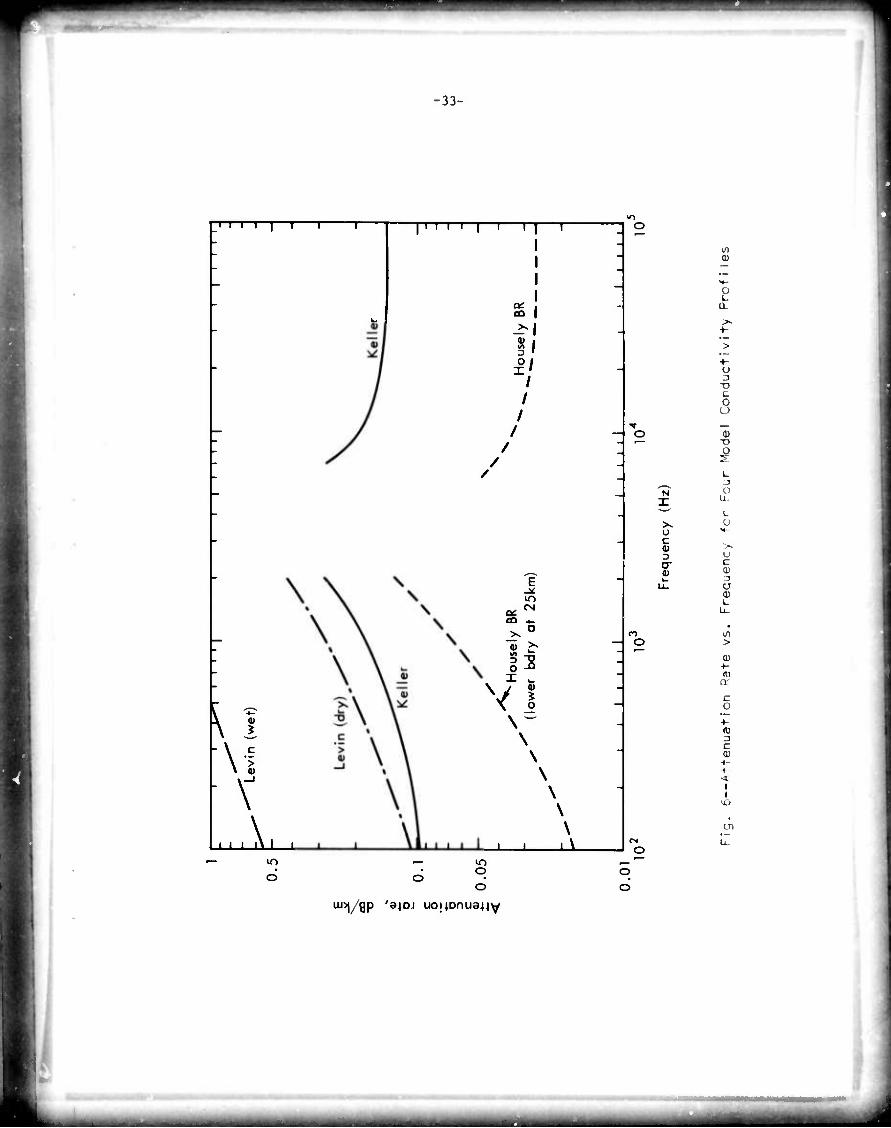
Figure 6 shows the calculated attenuation rates corresponding to

the various model conductivity profiles. Results are shown only for the

least-attenuated waveguide modes; viz., the TEM mode for 'requencles

lower than 3 or A kHz, and the lowest order TM mode for higher frequencies.

The results «howed that Includion of only these modfa Is adequate for

determining maximum transmission ranges. The decision to restrict

attention to frequencies between 100 Hz and 100 kHz was somewhat, but

not entirely, arbitrary. It is very difficult to radiate useful

amounts of power at frequencies as low as 100 Hs:. At frequencies

higher than about 100 kHz, the computational methods used here become

inconvenient due to the necessity of r« .aining large numbers of wave-

guide modes rather than the one or two least-attenuated ones. Ray-

tracing methods are probably preferable to modal analysis at these

higher frequencies. Also, the degrading effects of scattering from

irregularities in the crust would be expected to become more pronounced.

Nonetheless, it could well prove worthwhile to extend consideration

to frequencies outside of the ELF/VLF/LF bands treated here.

mm

■""• ■■■ m um -'*m^**^mmmmi^^i*m.'^m>m^~**i^**mmmmmim'W*frmmmriiimmm

-33-

i i i i—|—i 1 i

\

\1 V

■ ' ' \

i i i i i—i—r-i—r

CQ

81 u I I I

/

J I

E -^ ^o

Cki CN

CQ *- X

o

0) wo 13 o 5 X k-

V 0)

o

\ —

\ \

J L

O

IT) o

X

X u c S cr

O

tN O

o o

0

8

u

C

0 O

l

o U

L o

u c 1)

□ L.

u.

> a- ♦

ir

o

0) 3

0) •i + 4

I I

(i,

Lu^j/gp 'ajoj uoj4Dnua.ny

,_, . . - _ ....

—.—

-14-

The results shjwn in Fig. 6 apply to propagation in the continental

lithosphere, since a transition to free space was assumed at z-O (Fig. 5).

Attenuation rates were also calculated for the case where the crust

interfaces with sea water (approximated by a perfect conductor) at z«0.

These results, which will not be presented in detail, are virtually

identical to those shown in Fig. 6 for frequencies highf: than a few

hundred Hertz. At lower frequencies, the effect of assuming a sea-water

"top" on the waveguide is to reduce the attenuation from the values shown,

particularly for the Keller and Housely BR models. This behavior is to

be expected since, for extremely low frequencies where the skin depth

is large, sea water reflects energy that would otherwise leak out of the

waveguide.

The general dependence of attenuation on frequency, as shown in

Fig. 6, is quite similar to that observed for long-wave propagation in

the earth-ionosphere waveguide; viz., relatively low attenuation at

frequencies less than a few hundred Hertz or higher than 10 kHz, and a

"forbidden" band in the l-to-5 kHz portion of the spectrum. However, in

the earth-ionosphere waveguide, the attenuation rate is typically 2x10 "

-3 to 4x10 dB/km in the VLF band. And the attenuation seldom exceeds

_2 10 dB/km, even under disturbed ionospheric conditions. By comparison,

the computed attenuations in the lithospheric waveguide are an order of

magnitude or more larger.

The fact that the attenuation depends strongly on the minimum

value of conductivity and the conductivity depth-gradients is clearly

illustrated by the results shown in Fig. 6. The minimum conductivity is

The reader is cautioned against applying these results to propaga- tion under the oceans, however, since the models shown in Figs. 1 through 3 were developed to represent the continental lithosphere.

--•J - -

P9PH«>BI. iiiiii mi . «ftrmwmm^^jm^

•35-

about 10~ mhos/m for the L.»vin (wet) model, about 10 mhos/m for both

the Levin (dry) and Keller models, and about 5x10 mhos/m for the Housley

BR model. As would be expected, the Housley BR model yielded the lowest

attenuation, whereas that yielded by the LevJn (wet) model was by far the

hxghest. However, the attenuation rates for the Levin (dry) model and

the Keller model are quite different, even though the minimum conductivity

is nearly the same for the two models- At a frequency of 1 kHz, the

calculated attenuation rate is about 0.18 dB/km for the Keller model and

about 0.28 dB/km for the Levin (dry) model. The more favorable attenuation

in the Keller model of the lithospheric waveguide is due in part to the

assumed presence of a rapid transition in conductivity at a depth of

about 14 km (Fig. 2).

It is interesting to ccnpare the results shown in Fig. 6 with the

attenuation rates computed by Spiei and Wait (1971) for a step-function

model of the conductivity depth-profile. For an assumed waveguide

conductivity of 10 mhos/m, their calculated attenuation rates are

typically a factor of two or three lower than those shown in Fig. 6

for the Keller and/or Levin (dry) models. Thi:8e lower attenuation rates

are due largely to Spies and Wait's use of sharp, highly reflecting upptr

and lover boundaries rather than the gradual "boundaries" used here. Of

course, the conductivities used by Spies and Wait in their step-function

representation of the waveguide are intended to be "effective" values,

averaged over some appropriate range of depths, rather than minimum values.

In this context, the effective conductivity of the Keller-model waveguide

would be, say, 5 or 6x10 mhos/m, even though the minimum conductivity

is about 10 mhos/m.

-'■■■■- ..M^alHlMM

— ,.. r ,_ _... .,. IIIH IIH ■ I

-36-

The significant effect of conductivity depth-gradients, and the

presence or absence of sharp transitions in the conductivity depth-

profile, can be illustrated by examining the Housley BR model more

closely. For reasons discussed in Sers. II and III. the results

shown in Fig. 6 are not computed for the Housley BR model precisely

as shown in Fig. 3 (p. 13). Instead, the conductivity values shown

are used for depths down to 25 km, where a sharp transition to a highly

conducting sub-basement (i.e., a highly reflecting "boundary") is

assumed. As a check on sensitivity, additional calculations of the

attenuation rates for the Housley BR model are carried out for assumed

lower "boundary" depths other than 25 km. Sample results are given

in Fig. 7 for a frequency of 1 kHz. The attenuation is seen to

increase markedly as the assumed layer depth is increased. Results

corresponding to the Housley BR profile, precisely as shown in Fig. 3,

can be obtained by taking the depth of the assumed "boundary" to be

infinite. For this case (see Fig. 7), the attenuation rate is about

twice as large as when the profile is terminated at 25 km, and is

nearly as large as for the Keller model (see Fig. 6). Of course.

If the assumed transition at U-km depth were removed from the Keller

model, or if it were assumed to occur at a greatev depth, then the

calculated attenuation rates would be larger than shown in Fig. 6.

*It should not be inferred from Fig. 7 that the placement of the reflecting layer at a depth of 25 km causes the results shown in Fig. 6 and o be shown below in figures for the Housley BR model) to be unduly

optimistic. It can be inferred from seismic data that, ^ "«* 'JJ10"' a highly reflecting transition exists at depths shallower than 25 km. in whicf.Le the Housley BR results would be more favorable than those on

whicn the conclusions of this report are based.

m

—- iwwuiHiiu •^^^mm^nmmrnmmiimm miWli™''™*^****m*l'*w****nm^***^l^m*'^^**w™****mrmm***™mr***~

■37-

0.14

0.02

J L J L_^ 25 26 27 28 29 30 31 32 33

Depth of lower boundary (km)

CO

Frequency i kH2

oo

Fig. 7--Attenuation Rate vs. Depth f Assurr-ed ih^rp Transition in Conductivity (Housley Bf! Profile)

11 ) w JW^PI^P^BWWPWWJIJII HI .wmmmei

-38-

SIGNAL AND WISE FIELD-STRENGTH PROFILES

Equations (13) through (15) have been integrated to obtain the

field-strength profiles associated with the least attenuated waveguide

modes. Figures 8 and 9 show sample results, illustrating the calculated

field-strength profiles for the Keller model and frequencies of 1 kHz

(TEM mode) and 10 kHz (TM mode). Recall that in all cases the fields

are normalized such that V= 1 at the "center" of the waveguide; i.e..

at the depth of minimum conductivity. Thus, for the Keller model. V

has been set equal to unity at a depth of about 10 km.

One of the goals of this study is to estimate the dependence of

expected system performance on the burial depth of the receiving antenna.

Thus, for a vertically oriented E-field receiver-the configuration

assumed for illustrative purposes-the depth dependence of ^J is of

particular interest. Figures 8 and 9 show that IEJ has a broad

maximum centered at a depth of about 10 km. However, for depths shallower

than 5 or 6 km, |E I decreases rapidly as the depth is decreased. This

behavior, which is characteristic of a trapped mode in a waveguide

"centered" at a depth of 10 km, is due to four physical effects:

1) energy is absorbed as the signal propagates upwards toward the

earth's surface; 2) the conductivity and, hence, the admittance of

the medium increases as the depth is reduced-causing the electric

fields to be .educed relative to the magnetic field; 3) the signal

suffers gradient reflection as it "tries" to propagate upwards; 4)

since the refractive index increases as the depth is reduced, the

mmmm W—m w^mmmnmm

-39-

T—r—•—i—*—r

N

i

o

L. 0

s

r CL ^_ f * Q

(U • t M * >

X) L/1

(U r

^-k- C7) c

TJ a) 0) u N 4-

LO

D E TJ

I- o 0)

Z u. T3 0) N

I I

a)

en

UJ>I 'mdaQ

- - .. . . ,, ,^ M.

"■■I" " ■" "■" ——■^•■■p •-»-w—

-40-

N

s c I

» 0) u

$ u 1 0)

0) v"

— t/l £

-C +- Aa CI D5 0) C ( 1 (U k-

M U)

-o >

- 0) (A C

'o •*■ * p^ cn

■o e a 0) i- +-

D LTl

E o

X»

Z 0)

u

■p 0) N

cs _ o i

-9 ON

•

'o

. I

-41-

"wave" normal becomes more nearly vertical as the signal propagates

upward. This effect causes |E | to be reduced relative to both \E^\

and I*/" |. For depths greater than about 4 km and the two frequencies

corresponding to Figs. 8 and 9, |E I is greater than JEJ, which

indicates a signal traveling mainly in a horizontal direction. At

depths shallower than 4 km, the propagation direction has become more

nearly verUcil than horizontal. Of the four effects described above,

absorption becomes relatively more important as the frequency is

increased, since the skin depths are reduced, as are the admittances

and refractive indices.

Figure 10 shows the frequency dependence of the relative vertical

electric field strength ^ several depths for the Keller model. As

indicated on the figure, the relative field strength is normalized to

unity at a dep. of 10 km. As would be expected, the relative field

strength becomes smaller as the depth becomes shallower. Field-strength

profiles have also been calculated for the Housely and Levin models,

but in the interest of brevity are not presented in detail. For depths

shallower than about 10 km, the field-strength profiles based on the

Housley BR model are very nearly the same as those shown for the Keller

profile. This similarity is to be expected, of course, since the

conductivity profiles in the two models are identical for most of the

0-to-10 km depth range. On the other hand, the Levin (dry) model is

This interpretation is intended solely to provide an intuitive understanding of the numerical results and should not be taken too literally. Strictly speaking, of course, the concepts of wave normal and propagation direction do not apply when the medium has large spatial

gradients, as is the case here.

ttmmm- ,, .. -._ .— .- - ■ inmiiiililiBi lium -fiim ml i - -- —

"—■"■"" ' -■■■"'

■42-

-i 1—r | i mi T—r | i i 111 1—i—i iMii

Depth 10km

10

N \ \ \ 4km

■ i I I l > l i i I I I I 11 J I—I i I ll.

10 103 10

Frequency (Hz)

10"

Fig. 10—Relative Vertical Electric-Field Strength vs. Frequency for Several Depths (Keller Profile)

mmm^immagimmm^^m^mm^ ■ -

wmmm^m '"' " piiwipi 'mm win ■ ■■ —.■■w.-™- ii . • ii u.n

-43-

seen (Fig. 1, p. 9) to be much more highly conductive than either the

Keller or the Housley models for depths shallower than about 8 km.

Consequently, for depths shallower than 8 km, the relative field

strengths for the Levin (dry) profile are orders of magnitude smaller

than those shown in Figs. 8 through 10.

Noise-transfer functions have been computed from Eq. (18).

Figures 11 and 12 show |Y | and |Y | as a function of depth for the

Keller model, and frequencies of 1 kHz and 10 kHz. Recall that the

surface-noise fields shown in Fig. 4 should be multiplied by |Y | or

|Y | to obtain the vertical or horizontal electric-noise fields,

respectively, at a given depth. The noise propagates downward from

the earth's surface, whereas the signal propagates upward Tand laterally)

from the center of the waveguide. Thus, absorption and reflection tend

to reduce |Y2| and |YJ as the depth is increased. This behavior is

different than noted above for the signal fields, which suffer reflec-

tion and reflection losses as the depth is decreased. These state-

ments do not Lnply that the transfer functions must necessarily decrease

monotonically with increasing depth. As illustrated by Fig. 11, for

example, refractive effects can be dominant at the lower frequencies

and actually cause |Y | to have a larger value near the center of the

waveguide than near the earth's surface. Further, since the conduc-

tivity becomes low near the center of the waveguide, the crust becomes

quite transparent at these depths and standing wave patterns in the

transfer functions can occur. An example of such a pattern is shown

in Fig. 13.

^^^^^^MMÄ^^^^^^^^^^^tM|^^^t^_(Ä^^^^^^^ , .. ., .,.. .■■_._. _.

mmmmmim*mimm.i mmmym *jmm*mm^mmmmm rwmmnimmmmi mmm i

-44-

■«—i—'—r -'—I—r—r T—:

n >-

\ _ 'O

J L 04

-1_ I co

LU>| 'Lj4dao

o c

8

o Z

- 'O

p u

o

> in c O

0) -*- c E I-

i, i

!

■ I !■ «M^l ll - -

mji j i p ■^^»•^^wwiwB^wfl^xw^r

-45-

0 T 1 1 | I I I l|

Q.

Q

6 -

10

12

14 10

n

•TTL--- I 1 1 I I M I

103 10

Noise-transfer functions

I i i I i I i i

10

Fig. 12—Noise-Transfer Function vs. Depth (Keller Profile, 10 kH?)

MÜMMMriMMÜ ■BHU^HMMMM^MHR Au

-46-

Figures 11 and 12 show that JY^ is considerably smaller than

|Y 1 for most depths of interest. This behavior was found to occur

for essentially all of the models and frequencies for which calculations

were made. Thus, at least for the models used here, the vertical noise

electr.c-field component is typically murh smaller than the horizontal

one; and a vertically oriented electric antenna should therefore be less

severely degraded by atmospheric noise at depth than a horizontally

oriented one. This distinction has often been overlooked (e.g., GallaUa

and Haidle, 197?), and occurs simply because low-frequency electromag-

netic waves tend to be refracted strongly toward the vertical upon

entering the earth from free space.

The frequency dependence of the noise-transfer function of interest,

lyj, is shown in Fig. 13 for the Keller model at several depths. At 2

the lowest frequencies considered, the vertical component of atmospheric

noise tends to increase with increasing depth, indicating a dominance

of refraction over absorption. Thus, somewhat surprisingly, the vertical

component of atmospheric noise at ELF is found to be stronger at a depth

of 1C km than at a depth of, say, 2 km. Of course the total normalized

noise power decreases more-or-less monotonically with increasing depth.

At the higher frequencies, |Y2| is seen to decrease ar the depth is

increased, iniicating that absorption is the dominant mechanii Ism

determining field strength,

DEPENDENCE OF S1GML-TO-NOISE RATIO ON RECEIVER DEPTH

We next consider the depth-degradation factor, D(z), which is

simply the ratio of the signal-to-noise ratio at a given depth to that

- - -- ■ — . .

mmmmmmm

— wKwii«<i.a.jiiwim>i>^WMii .^iMiiiPf|Hi>W!V^^PllH'- l"L-

-47-

10 C 1 1 1 I I I M| 1 1 I | I I M| 1 I I | M I L

Depth = 10km

10 -5 I ■ ■ i i i i il ■ ■ i ■ ■ ■ ii 1 1—l I MH

10' 10' 10' io-

Frequency (Hz)

Fig. l3--Noise-Transfer Function (Vertical E-field) vs. Frequency for Several Depths (Keller Profile)

-— w«< P"W"^«wM«i^Vippppi|P|PMiPllllpnnF«OTW.i .iiiiiHiiii.>mipHPi^n*mp^Mi^

-48-

at the nominal center of the waveguide. Thus, in the Keller model,

for example, D(z) is the power required to transmit to a receiver at

a depth, z, divided by the power required to transmit to a similar

receiver buried at a depth of 10 km; i.e., D(z) is the factor by which

the transmitter power must be changed if the receiver is moved from

a 10-km depth (Keller model) to some other d«pth. Since 10-km deep

holes are very expensive to bore, we are particularly interested in

determining the additional power that would be required if the receiver

were placed at some lesser depth.

For all of the models considered in this report, atmospheric noise

dominates the thermal noise for all depths and frequencies of interest.

Thus, the simplified Eq. (35) may be used, and D(z) expressed solely as

a function of the signal field-strength profiles and |Y2|. Some examples

of the depth-degradation factor are given for the Keller model (1 and

10 kHz) and the I.evin (dry) model (1 kHz) in Fig. 14. For the Keller

model, which exhibits a fairly constant conductivity depth-gradient

between 0 and 10 km, relatively little degradation would be suffered

by reducing the receiver depth from 10 km to. say, 5 or 6 km. Moreover,

as discussed below, the penalty in transmission range is remarkably

moderate even for receiver depths as shallow as 3 km. As indicated

earlier, «"he Levin (dry) model exhibits a rather large and abrupt

This dominance occurs because, even after allowing for losses suffered in propagating from the earth's surface to the nominal center of the waveguide, the atmospheric-noise density was found to be stronger than the thermal-noise density. It is, of course, possible to envision realistic situations in which the atmospheric noise would be so highly attenuated as to be no longer dominant. A case in point would be if the receiver were situated in the suboceanic lithosphere.

-49-

i 1 r

N

Q

o o o

t 1 ■•-

CL 0)

Q

J I 1—L CN ^t O

oo J.

'D

U1 >

c O

TO TO

a

!

n.

mm iwmwti^m^immmnmmif^^mmfrmmwf^

■50-

increase in conductivity as the depth is reduced to less than about

8 k..* A major result of this assumed transition in conductivity is

illustra-.ed in Fig. U; D(z) becomes so large as to essentially rule

out any possibility of using a receiver depth shallower than 7 or 8 km.

Thus, to the extent that borehole depth affects total system cost, the

attractiveness of a lithospheric communication system depends quite

strongly on the gradient of conductivity in the crust at depths between

0 and 10 km.

Figure 15 shov, the frequency dependence of D(.) for Che Keller

.odel and aeverel depche of incereet. Of cour.e. DW-l ac a depch of

10 to. Aa «Ighc he expecced, higher frequency slgn.U are much „ore

sensidve to receiver hurial depth than are lover fre.uency ones. The

large Increaae in DU) for ahallov deptha exhihited at frequenciea

Mgher than 10 .Hz la due to two factora: 1) the aignal geta vea.er

M the aurface of the earth ia approached, due to absorption auffered

in propagating upward fro« near the center of the waveguide; 2) the

.tn,oapheric noise geta stronger near the earth's aurface. since the

shaorption It suffers In propagating downward la reduced. For reaaona

given above, Dfx) for the Housley BR »odel Is very nearly the same as

that shown in Fig. 15, whereas that for the Levin .odel la prohibitively

Urge at depths ahallower than 7 or 8 km.

TMjgiaioH "A"0" as ?"u™ |!EO"'

REME''

TS

The dependence of required power on data rate, transmission range,

transmitter efficiency, frequency, and receiver burial depth haa been

W^ehavior would be expected in regions having a thick, highly

conducting, sedimentary layer.

--

<iw*v-*n ijuuuiwpiifannpHiiqpii*«'** «.ii ni'» .rwi^ip^p^p)!

-bi-

10 c 1—i i i i mi 1—i i I i mi 1—i i I i lit

10'

Receiver depth = 2km

N Q

S 10:

u

■t-

I 102

l

10

2k m

•^ 3km

s.

3km

A---

/

4km

■ ■ ■ i ■ i ui i—i i I i ml 1—i—L-L

10' 103 104

Frequency (Hz)

10"

Fig. 15—Depth Degradation vs. Frequency for Several Receiver Depths (Keller Profile)

^^_^, ^>aj*aai^*in i i iniiiB^i ■• ._-^,.-^—J^... ....... . m.nK-gi...

— k^MP^^^P"

-52-

calculated from Eqs. 32 and 33. Values for ms atmospheric noise corres-

ponding to Colorado summer are taken from Fig. 4. (p. 15). As discussed

in Sec. II, the use of rms noise spectra Implies a system time avail-

ability of 80-to-90 percent. Also, we assume no processing gain, and

have thus taken Gp equal to unity. This assumption is probably quite

conservative, since 10-to-20 dB of noise suppression can typically be

achieved in above-ground VLF/ELF systems {Evans and Griffiths, 1972).

If. say, 10 dB of noise suppression can be achieved in a lithospheric

system, then the power requirements given below would suffice for a

time availability approaching 99 percent, rather than the above-stated

80-to-90 percent. For purposes of presentation, it is convenient to

define a normalized, required effective power (REP) as follows:

n P REP req

(Watts), (37)

Where Preq is the total Power that must be delivered by the transmitter,*

as computed from Eq. (33). The transmitter efficiency, n, denotes total

efficiency; viz., the ratio of the power radiated into the least-

attenuated mode to the total system power; n thus accounts for antenna

radiation efficiency, the excitation efficiency of the dominant wave-

guide mode, transmission line losses, etc. Therefore, REP denotes

* Strictly speaking, REP has units of Joules/bit, rather than Watts,

since R has units of bits-per-sec, and n is dimensionless. The distinc- tion vanishes for a data rate of 1 bps, since the energy per bit is tnen numerically equal to the power. A more precise definition than given by Eq. 37 would be

n R REP

req

where R0-l bit-per-second. In the following discussion and figures, the factor RQ is suppressed, and REP will be expressed as the effective power required to transmit 1 bit-per-second.

_ mmvemmmmUHtm*

«IWPWPni^IRPRIVMVPPPnPPnnaiw^i^PiMi^ -. - -.

-53-

the power that must be radiated Into the dominant mode to achieve a

data rate of 1 bit-per-second (bps). REP is a convenient parameter,

since It is independent of n (see Eq. 32). which is extremely difficult

to calculate for a transmitter in an inhomogeneous conducting medium.

It is. of course, a simple matter to compute the required power. Preq,

from REP. once n has been calculated and a data rate. R. chosen.

The transmitter efficiency, n. cannot now be specified accurately.

However, some assumption must be made regarding achievable transmitter

efficiencies if system feasibility and attractiveness are to be assessed

quantitatively. To undertake such an assessment, we assume, without

delving into the specific transmitter configuration, an efficiency

that, based upon present understanding, does not appear to be unduly

optimistic. Specifically, in addition to detailed calculations of REP.

results will be given for Preq for the case whe: e n/F = 10 ; i.e..

where the total required power exceeds REP by a factor of 1000. This

choice is by no means arbitrary. Gallam and Haidle (1972) have

estimated that efficiencies of a few percent should be achievable for

a VLF transmitter utilizing a deeply buried vertical antenna. Thus,

at VLF. our choice of n/R-10'3 can be interpreted as corresponding to

an efficiency of a few percent and a data rate of a few tens of bps.

Of course, for poorer efficiencies, such as would probably occur at

the lower frequencies considered, the data rates would be proportionately

lower. Although we consider n/R-lo"3 to be a reasonable choice for

the purposes of this study, other values could equally well have been

used. Fortunately, the main conclusions do not depend strongly on

the precise value of n. Moreover, since extensive graphs of REP are

_ „.^

■— ,' iiiiiiiiwmwmiinn-i' • —'■"" i

-54-

given below, total power requirements can be obtained for any

efficiency and data rate: simply multiply REP by R and divide by n.

Figure 16 shows REP as a function of transmission range for several

frequencies and the Keller model. For comparison, REP for the Levin

(dry) model Is shown for a frequency of 1 Hz. The results shown In

Fig. 16 apply to the situation where the receiving antenna Is located

near the center of the waveguide—about 10-km deep for ihe Keller model

and about 9-kni deep for the Levin (dry) model. Also shown In Fig. 16

(right-hand axis) Is the total required system power for combinations

* -3 of efficiency, n, and data rate, R, such that n/Rm10 . Any effects

of transmitter burial depths are Included Implicitly in the efficiency.

Several important conclusions can be drawn from Fig. 16. The

higher frequencies considered are clearly superior to the lower ones,

as evidenced by the fact that, for a given power, far greater ranges

are achievable at 5'J kHz than at the other frequencies shown. This

superiority is almost entirely due to the quieter noise environment

at 50 kHz and a depth of 10 km. Reference to Fig. 13 shows that, for

a depth of 10 km, the noise-transfer function. If-li decreases strongly

and monotonlcally with increasing frequency. Actually, the superiority

of the higher frequencies is probably even more clear-cut than shown in

Fig. 16—it should be easier to achieve n/R-10 at 50 kHz than, say, at

1 kHz, since antenna efficiencies typically Increase with increasing

frequency.

We do not imply, of course, that n will be Independent of frequency and receiver burial depth.

,__^^M^^^tf^^^Hi^HHWHi .., ■,- iiMMHHMllMliH ^^^^^^^M&^MM

Ifimii

■55-

200 300 400 500 600 700

Transmission range (km)

Fig. l6--TransmIssion Range vs. Effective Power and Total Power (Keller and Levin (dry) Profiles, 10-km Receiver Depth)

«■MMMaaauiM **m m*m

^^w^WWWW^WW"*"""""

•56-

For purposes of discussion, we assume that 10 megawatts is an

acceptable power requirement for a practical system. On this basis,

transmission ranges on the order of 1000 km appear achievable, provided

that the Keller (or Levin (dry)) model of the lithosphere is found through

field measurements to be a reasonably good representation. On the other

hand, the system power requirement based on the Levin (wet) model are

so high for transmission ranges of interest that the results are not even

worth presenting.

One very important general point should be toted: viz., the

system performance depends exponentially on signal- and noise-attenuation

rates, but only linearly on other parameters. Thus, the required power

at a given frequency depends linearly on n and R, and exponentially on

the transmission range, d. Conversely, achievable transmission range

depends only logarithmically on efficiency, data rate, and power. A

misleading impression can be gained if sysf»^ performance is assessed

on the basis of the power required to transmit to some specified range.

Instead, performance should be assessed on the basis of the range that

can be attained with some specified power. The following simple numerical

example will clarify the distinction: As indicated above fci the Keller

model, a range of 1000 km is attainable with a total power of 10 mega-

watts, provided that ri/R=10 . Assume, for purposes of discussion, that

future analysis shows that n/R=10 is the best that can be achieved.

If the 1000-km transmission range is regarded as specified, then the power

requirement increases to 100 megawatts, which is probably impractical.

On the other hand, if the 10-megawatt power is regarded as specified.

...^ÜHMlMi^»»..-.^—^-^- - -■- ■-

MmpmgB »^•■^»^- •■■i' in i.i. ij

-57-

then the ten-fold decrease In efficiency* causes the .axi.un. transmission

range to decrease to ahout 850 I--, penalty of only 15 percent.

Since system cost will depend greatly on the depth to which antennas

„ust be buried, we next consider the penalty in transmission range

(power being specified) that must be paid if receiving antennas are

buried shallower than the nominal center of the waveguide. Since

practical radio communication systems typically have many more receivers

than transmitters, receiver burial depth is probably a more important

consideration than transmitter burial depth.

Figure 17 shows, for the Keller model and frequencies of 10 and

50 .Hz. the dependence of required power on transmission range for several

assumed receiver burial depths. For a frequency of 50 .Hz and a total

power of 10 megawatts, the calculated transmission ranges are 700-to-800

to for receiver depths as shallow as 3 or 4 km. These ranges are only

20-to-30 percent less than those corresponding to a receiver depth of

10 km.** Since drilling costs are apt to be a large fraction of the total

system cost, a tradeoff of a 20-to-30 percent reduction in transmission

range against a factor of 3 reduction in borehole depth would seem

advisable. Such a tradeoff cannot be carried too far. however. For the

Keller model and a frequency of 50 kHz. use of a receiver d.i,th of only

2 km would cause the depth degradation function (Figs. U and 15) to

^T^uivalently. a ten-fold increase in required data rate, or

ten-fold decrease in allowable system power.

**ARain note the misleading conclusions that can be drawn ^ "ans-

mi3sionTainge. rather than power is considered to ^ -y. em P cifica

^^ttT-T^ 3 ^-l-i^ .increase in power

of nelrly 3 orders of magnitude (for the Keller model)!

mwinwui in'iw,-

1 '" ""■"«'«I

^

-58-

Transmissicn range

Power and Total Power Fi9- i7"rr.^rBn:.^rii::..r P™..,..

«■■■■■MMM

■II i m^-m vmi ^Kfh^aKM^bM^ftMgdM

■VWM'^iW»^"1

•59-

become so large that the corresponding reduction in transmission range

would probably be intolerable. Note also that for lower frequencies

(e.g., 10 kHz or less—see Fig. 15), the fractional degradation in

transmission range incurred by using shallow receiver depths is less

severe than at 50 kHz. Nonetheless, for depths greater than about

three kilometers, the higher frequencies are still preferable.

Figure 18 is completely analogous to Fig. 17 except that it applies

to the Housley BR (assumed transition at 25 km) model. Should this

model prove to be a reasonably good representation of crustal conduc-

tivities over large geographic regions, then transmission ranges

approaching 5000 km could be achievable for receivers placed at depths

of about ten kilometers. Even for receiver depths as shallow as 3 or

4 km, ranges in excess of 3000 km are a possibility. Again, frequencies

of several tens of kilohertz are preferable to lower frequencies.

Detailed results have not been shown for the Housley EUS model. The

achievable transmission ranges based on this model would be of the

order of 10,000 km.

We have not explicitly considered situations for which the litho-

spheric conductivity profi.1 e exhibits lateral variations over the propa-

gation path. Of course such variations would be expected to occur in

situations of practical interest; e.g., propagation between two geo-

logical provinces. Mode conversion caused by lateral variations is

not expected to be large anough to alter the main conclusion of this

study (Wait and Spies, 1972). Thus, the transmission through a

For a discussion of evidence that good lateral continuity does exist over large distances, see Heaaoak (2971), pp. 1-9.

.. BMMMH

l**^—"-j - ■ ■"• ^.. . .. .. ^»..^^^«tefaM -- - --- -

mi' iiiiiiiiiv^naiBnmppnmm^^w

I >

0)

-a

N

O Z

-60-

1000 1500 2500 3500

Trc.ismission range (km)

Fig. 18—Transmission Range vs. Effective and Total Power for Several Receiver Depths (Housley OR Profile)

mm

mm^mm^^*^m*mm*~~m* „„m ■'.» ■> i wmmmmmm^gH

-61-

non-stratifled lithosphere can be estimated reasonably well by simply

summing the attenuation suffered in each region, using the appropriate

attenuation rates (Fig. 6. p. 34) and path lengths. The depth-degrada-

tion factor, however, depends solely on the properties of the lithosphere

in the vicinity of the receiver.

The existence, or non-existence, of sharp transitions in conduc-

tivity on the bottomside of the waveguide can alter the maximum trans-

mission range by about a factor of two. An example of this effect is

given in Fig. 19, which shows the degradation in calculated transmission

range that occurs as the depth of the assumed lower reflecting layer

in the Housley BR model is increased beyond 25 km. Of course, improve-

ments would occur for shallower layer depths, as they would if either

the Housley EUS or SN profiles were used (Fig. 3, p. 13). Clearly,

field experiments (see Hales, 1972; Keller, 1972), as well as studies

of the relation of laboratory data to in situ rocks, must be undertaken

if these uncertainties are to be satisfactorily resolved.

In regions where the conductivity profile at depths shallower chan

8 km is similar to that shown by Keller (Fig. 2, p. 10) rather than

as shown by Levin (Fig. 1, p. 9), antenna burial depths of only 3 or

4 km should be adequate for a meaningful propagation experiment. As

Indicated by the results shown in Fig. 17, other conditions would also

have to be satisfied:

1) Combinations of transmitter efficiency, bandwidth (R), and

total power should be selected so that the power radiated

into the lowest TM mode is at least a few watts. (The

corresponding requirement for total powar could be well in

excess of a kilowatt.)

■ - - —

■»•—■' ' " ■ —

-62-

Q-

I > u 0)

-Ö <u

'5 cr 4) t-

"O (U

E o Z

200 400 600 800 1000

Transmission range (km)

1200 1400

Fig. 19—Transmission Range vs. Effective and Total Power for Several Depths of Assumed Sharp Transition in Conductivity (Housely BR Profile, 10-km Receiver Depth)

■ - - - —

in> wmm *\.m — IW.W«,^I. -

-63-

2) A frequency of several tens of kilohertz should be use.\.

As discussed by Levin (1972), a propagation experiment has been carried

out at a i equency of 2.2 kHz, a total power of 2.5 kilowatts, and with

3-km deep boreholes. The negative outcome of this experiment does not

provide conclusive evidence that favorable conductivity profiles are non-

existent in nature. The 2.2 kHz frequency was much lower than optimum,

and the antenna efficiency might well h-.ve been too poor to provide

adequate REP from the 2.5-kilowatt total power. Further, the 3-km deep

boreholes may simply have been too shallow for the particular region

where the experiment was carried out—deeper boreholes or a different

test site being needed. Clearly, very careful site selection and antenna

dodign are needed for a conclusive experiment.

I - - - . - .-. ^^.-^^^^^^^a^. ^m-.A^„ - ■■ ■ ■ ■-■■■ ■-■ ■- ^MkMi

,~-— "__.,

-64-

REFERENCES

Blackwell, D. D., "The Thermal Structure of the Continental Crust," The Structure and Physical Pvopertiea of the Earth's Crust, J. G. Heacock, ed., AGU Monograph 14, 1971.

Brace W. F., "Resistivity of Saturated Crustal Rocks to 40 km Based on'Laboratory Studies," The Structure and Physical Properties of the Earth's Crust, J. G. Heacock, ed., AGU Monograph 14, 1971.

Budden, K. G., The Waveguide Mode Theory of Wave Propagation, Logos Press, London, 1961.

Evans, J. E., and A. S. Griffiths, "Design of an ELF Noise Processor," Engineering in the Ocean Environment, IEEE Publication 72 CHO 660-1 OCC, 1972.

Field, E. C, "The Effects of Ions on Very-Low-Frequency Propagation during Polar Cap Absorption Events," Radio Science, Vol. 5, 1970.

Gallawa, R. L., and L. L. Haidle, An Engineering Feasibility Study of Communications via a Subterranean Waveguide, Institute for Tele- comnunication Sciences, OT/TRER 39, November 1972.

Hales, A, L., et al., A Multidisciplinary Program of Investigation of the Possibility of an Electromagnetic Wave Guide in the Lower Crust, University of Texa^ at Dallas (March 7, 1972).

Heacock, J. G., ed.. The Structure and Physical Properties of the Earth's Crust, AGU Monograph 14, 1971.

Housley, R. M., private conmunication, 1973; also, Simmons, G., R. M. Housley, and F. J. Forin, "Electrical Resistivity of Rocks and the Possibility of Lithospheric Comnunication," to be published, 1973.

Keller, G. V., "Electrical S udies of the Crust and Upper Mantle," The Structure and Physical Properties of the Earth's Crust, J. G. Heacock, ed., AGU Monograph 14, 1971.

Keller, G. V., et al., Recormendation of the Working Group on Electro- magnetic Methods (March 6, 1972).

Keller, G. V., private comnunication, 1973.

Levin, S. G., "Radio Propagation through the Crust-Retrospect and Prospect," The Structure and Physical Properties of the Earth's Crust, J. G. Heacock, ed., AGU Monograph 14, 1971.

Maxwell, E. L., "Atmospheric Noise from 20 Hz to 30 kHz," Radio Science, Vol. 2, June 1967.

immmi wmmmKmmr^ mmmmmm 1

-65-

K.iM K P and J. R. Walt, On Calculations of the Modal Pavametere ^ly^n IdealTL Ecn-th-Crust Waveguide, Institute for Teleconnnunlca-

tlon Sciences. Tech. Kept. N. 1. March 17. 1971.

Walt. J. I., "An Anomalous Propagation of Radio Waves in Earth Strat*."

Geophysias, 19(2), 195A.

ii.4* I R and K. P. Spies, On Mode Conversion in the Earth-Crust ^WaveguikeXst for Jele^unication Sciences, Tech. Rept. No. 4,

27 October 1972.

Wheeler. H. A.. "Radio Wave Propagation in the Earth's Crust," Radio

Sai.', 66D(2), 1961.

... . ^--gg^.-——ig--,^ [■■■laMWllrMiafc

11 -'>«•'"«nmuPMinpppmpwp I-'JIII.PII.PII ii .11 mm w«r^^ ' ""i11. ■ " > "

Unclassified Security Classification 2

DOCUMENT CONTROL DATA -R&D (Security flats./ir.Hon of fit)«, body ol abslrai I and ,nd**i„e muMUtlam mu»l he »nfered when Ihe uverall report U cletsllitd)

OHiGiNATiNG ACTIVITY ^Corporafe author) 'ia RtPOHT SECURITY CLASSIF1CA TION

Paclflc-Slerra Research Corporation 1456 Cloverfleld Blvd. Santa Monica, California 90404

Unclassified Zb. GROUP

NA 3 REPORT TITLE

ELECTORMAGNETIC COMMUNICATION IN THE EARTH'S CRUST

4 DESCRIPTIVE NOTES fTVf. ./reporf and (nclusive dale»;

Semiannual Technical Report S AU TMOR(S) (First name, middle initial, fast name)

Edward C. Field and Michael Core

8 REPORT DATE

June 29. 1973 •a. CONTRACT OH CHANT NO

N00014-73-C-0189 6. PROJEC T NO

ARPA Order No. 2270/8-16-72

Program Code No. 3F10

7a. TOTAL NO OF PAGFS

72

76. NO OF REFS

18 9a. ORIGINATOR-S REPORT NUMBERISI

PSR Report 306

9fc. OTHER REPORT NO(S) (Any other numberm (haf may be aetifned thie report)

IT DISTRIBUTION STATEMENT

ii SUPPLEISENT^RY NOTES

STATEMENT A| V

r«ismietal ot tMs JpcvwenC out#lde|the,agencies 6$ the U.S. /W- dek m* WVWi*^^*!^* Co&JV, OtUce o^val/^far2h.

12 SPONSORING MILI TARY ACTIVITY

Advanced Research Projects Agency 1400 Wilson Blvd. Arlington, Virginia 22209

13 ABSTRACT

This report presents results of an analysis of the capabilities that might be achieved with a litho-spherlc communication system. The analysis uses several avail- able models of contin*-^«! lithospheric conductivity as inputs to calculations of transmission characttv des and possible communication system parameters. Because of prevailing uncert*inti««, significant differences exie. among the various models; and a wide range of future sy.tem capabilities is found to lie within the realm of possibility. M. .. .

For all models used, the c.Mculated attenuation rates are considerably larger than for above-ground transmission, which depends on propagation in the earth- ionosphere waveguide. In spite of this fact, reasonably large transmission ranges might be possible in the lithosphere because the atmospheric noise fields at depth are very small, having suffered heavy attenuation in propagating downward from the earth's surface.

The major factor affecting bestem feasibility is whether water-saturated micro- cracks exist in aU 'Mjor rock types at depths ^reater than, say, 5-to-8 km. If such microcracks exist v.- assumed in on« model), and minimum conductivities in the crust exceed 10-5 - 10-6 „.hos/m, then the calculations show clearly that a practical com- munication system is not feasible. For this case, the attenuation rates are so high that only very short transmission ranges could be achieved, even if large amounts of power were expended. Field experiments will be needed to determine with certainty whether saturated microcracks are, in fact, present at the depths of Interest.

SEE ATTACHED PAGE

DD .FN0ORVMJ473 Unclassified Security Classification

■-... -■ — - ... ■■ ■ ■ :^A.

' ainn Hi.(».in i^l pmii^p« II.«M^> ! jj^^tnv^w^

Ilnclassifled Security Classification

KEY WO R D»

lithosphere

communications

military communications

very-low-frequency propagation

Unclassified Security Classification

. ^—»-. ^^^^^^^^^v^M^^^^^^^^^^. ^...-.... ^.■■J,„_.>. ^ ^-.,.. ..^JJ^i^JllM>«»aMi«^M—MIIH

m^m^m^m ill ■■Main.

CONTINUATION OF ABSTRACT

However, valid reasons exist for optimism that fluids (or fluid films) should not be an important factor at depths greater than several kilometers, and that conductivity profiles (at depth) based on labora- tory data for dry rocks more closely approximate actual conditions. Further, recent laboratory data indicate that the conductivity of dry rock in the crust could be much lower (lO-8 to 10~9 mhos/m) than previously believed (10~7 mhos/m). It is, of course, difficult to relate data obtained from laboratory samples to conductivities of L-ock in situ. Nonetheless, calculations using conceptual profiles based on the assumption of dry basement rock yield results that are quite encouraging. For example, for data rates of a few tens of bits- per-second and power expenditures of l-to-10 megawatts, transmission ranges of from about 1000 to many t> ousands of kilometers (depending on the profile used) appear to be a possibility.

The calculations show clearly that much larger transmission ranges can be achieved in the LF band (30-100 kHz) than at the lower fre- quencies considered. This »ffect is due mainly to the heavy attenua- tion suffered by downward propagating atmospheric noise at the higher frequencies. The calculations also show that the maximum transmission ranges are somewhat sensitive to the details of the model profiles. For example, for two profiles exhibiting the same minimum conductivity, the transmission range (for a specified power, etc.) can vary by a factor of two depending on the conductivity depth-gradients, and the precise location of any sharp transition layers that might exist.

The depth to which a receiver must be buried to achieve satisfac- tory performance is a particularly important parameter, since borehole drilling costs could be a large fraction of the total system cost. The transrcibslon ranges given above apply when the receiving antenna is located near the "center" of the waveguide—assumed to be about ten kilometers deep for the conductivity profiles used in this report. For profiles representative of regions stripped of highly conductive sedimentary layers, the calculations show that receiver depths as shallow as 3 or 4 km couj.d be used at only a 15-to-20 percent penalty in transmission range.

- ^.——^-^_,

'■"''" ^W-™WP-—— ■ • ' -1 • lll.Klil —

DISTRIBUTION LIST

Director Advanced Research Projects Agency 1A00 Wilson Boulevard Arlington, Virginia 22209 Attention: Program Management

Defense Documentation Center Cameron Station Alexandria, Virginia 2231A

ST01AC Battelle Memorial Institute 505 King Avenue Columbus, Ohio 43201

Office of Naval Research 800 North Qulncy Street Arlington, Virginia 22217 Attention: Code A17

2 copies

12 copies

1 copy

3 copies

Office of Naval Research 1030 £. Green Street Pasadena, California 91106

Commander, Defense Contract Administrative Services District, Los Angeles

11099 So. La Cienega Blvd. Los Angeles, California 90045 Attention: DCRL-DLCB-C4

1 copy

1 copy

Director Naval Research Laboratory Washington, D.C. 20390 Attention: Code 2629

6 copies

Director Naval Research Laboratory Washington, D.C. 20390 Attention: Code 2627

6 copies

HI

iwmm^mmmm

Office of Naval Research 800 North Quincy Street Arlington, Virginia 22217 Attention: Dr. Sidney G.

Dr. Thomas P. Dr. Robert G.

Reed, Jr., Code 102T Quinn, Code 418 Morris, Code 421

Director Naval Research Laboratory Washington, D.C. 20390 Attention: Mr. William E. Garner, Code 5460

Dr. John Davis, Code 5464 Dr. L. B. Wetzel, Code 5400

Defense Communication Agency 8th and S. Courthouse Road Arlington, Virginia 20390 Attention: Capt. Richard ?. Gardiner, Code 960

Dr. Samuel Koslov, OASN (R&D) Room 4E741 Pentagon Building Washington, D.C. 20350

Chief Scientist, Code 0P094H Command Support Programs Room 4C558 The Pentagon Washington, D.C. 20350

Naval Electronic Systems Command Special Communications Project Office

National Center //I Arlington, Virginia 20360 Attention: Mr. John E. Doncarlos, PME 117T

Deputy ASSIF int Secretary (Systems) OSD(T) Room 3D174 - The Pentagon Washington, D.C. 20350 Attention: Dr. Howard L. Yudkin

Deputy Director Strategic Submarine Command and Control Program Office Room 5D584 - The Pentagon Washington, D.C. 20350 Attention: Capt. William H. Lynch, Code 0P094RB

Foreign Technology Division Wright-Patterson Air Force Base

Dayton, Ohio 44223 Attention: Capt. John D. Mill (USAF)

«^ M

laniu «luu.?'

Mr. Edward J. Kolb Naval Security Station 3801 Nebraska Avenue, N.W. Washington, D.C. 20390

Mr. Clarence Sargent Room 4G0A CIA Headquarters Washington, D.C. 20505

U.S. Army Electronic Command Headquarters Ft. Morwouth, New Jersey 07703 Attention: Mr. Morris Acker

Mr. Finn Bronner Army Research Office Durham, North Carolin

Dr. James R. Wait Environmental Research Labatories U.S. Department of Commerce Room 231, Research Building //I Boulder, Colorado 80302

Dr. Robert L. Gallawa Office of Telecommunications Institute for Telecommunication Sciences U.S. Department of Commerce Boulder, Colorado 80302

Dr. D. D. Crombie Associate Director Institute for Telecommunication Sciences U.S. Department of Commerce Boulder, Colorado 80302

Mr. Frank Finlan Ordnance Research Laboratory Pennsylvania State University State College, Pennsylvania 16802

Commander H. E. Sprecher, Jr., Code 543 Naval Ordnance Systems Command National Center //2 2521 Jefferson Davis Highway Arlington, Virginia 20360

Professor Charles S. Cox Scripps Institution of Oceanography University of California La Jolla, California 92037

a^^Mat^u. ._.._._ ^^

m^****w^m "" "■^"

Professor Gene M. Simmons Department of Earth and Planetary Sciences Massachusetts Institute of Technology Bldg. 54-314 Cambridge, Massachusetts 02139

Professor George V. Keller Colorado School of Mines Golden, Colorado 80401

Dr. Robert M. Housley Science Center Rockwell Internationa] Planetary Physics P.O. Box 1085 1049 Camino Dos Rlos Thousand Oaks, California 91360

Professor Stanely H. Ward Department of Geological & Geophysical Sciences

University of Utr.h Salt Lake City, Utah 84112

Geomagnetlcs and Electrical Geosclence Research

Laboratory Engineering-Science Bldg. 623 Austin, Texas 78712 Attention: Professor H. W. Smith

Professor F. X. BosticK

Professor R. B. Smith University of Utah Department of Geo. oglcal & Geophysical Sciences

Salt Lake City, Utc'h 84112

Professor Mark Landisman Geosciences Division University of Texas P.O. Box 30365 Dallas, Texas 75230

Mr. Robert A. Moore Office of Defense Research & Engineering

Room 3E129 The Pentagon Washington, D.C. 20030

Mr. P. Haas Defense Nuclear Agency Washington, D.C. 20305

Mr. D. Evelyn Defense Nuclear Agency Washington, D.C. 20305

■■- ■ ■ -- . . _ __ - ■ - ■

.___-__ _^

~>K**mmm

Mr. W. Hei.iig Defense Communications Agency Washington, D.C. 20305

Dr. W. A. Decker P.O. Box 1925 Main Station Washington, D.C. 20013

Defense Intelligence Agency Washington, D.C. 20301 Attention: DIADT

Dr. B. Krueger Naval Electronics Systems Command Department of the Navy Washington, D.C. 20360

Mr. Dan Barney Code 53212 Naval Intelligence Systems Command 1136 Hoffman Building Alexandria, Virginia 22314

Mr. Jerry Batts (NISC-42) Naval Intelligence Support Center 3201 Suitland Road Washington, D.C. 20390

j

i Dr. E. Lewis Air Force Cambridge Research Laboratory L.G. Hanscom Field Bedford, Massachusetts 01730

Colonel E. C. Mixon DCS/Research & Development Headquarters, USAF (AFRDQ) Washington, D.C. 20330

Mr. T. Kamm Air Force Weapons Laboratory Kirtland Air Force Base, New Mexico 87117

Dr. Robert Jones Foreign Science tt Technology Center Charloutsville, Virginia 22901

i ■M»«M ___

"•—•"■'' mmmm

Dr. A. M. Peterson Stanford Research Institute 333 Ravenswood Avenue Menlo Park, California 9402b

Dr. A. Fraser-Smith Stanford University Stanford, California 94305

Dr. C. Greifinger Research & Development Associates 525 Wilshire Blvd. Santa Monica, California 90403

Mr. D. H. Blumberg Computer Science Corporation 1095 Duane Court, Suite 211 Sunnyvale, California 9'>08b

Mr. M. D. White Massachusetts Institute of Technology Lincoln Laboratory P.O. Box 73 Lexington, Massachusetts 02173

Mr. Mario Grossi Raytheon Company 528 Boston Post t.oad Sudbury, Maryland 01776

Dr. K. Powers Research Corporation of America 301 Ridgeview Road Princeton, New Jersey 08540

N

f ■ ■ -— — -

M