UNCLASSIFIED

AD 26 503

ARM ED) SERVICES TECHNICAL INFORMATIOK MENCTARLING1N HALL STATIONARLINGTON 12, VIRGINIA

UNCLASSIFIED

NOTICE: When goverunt or other dravings, speci-fications or other data are used for any purposeother than in connection vith a definitely relatedgovernment procurement operation, the U. S.Government thereby incurs no responsibility, nor anyobligation whatsoever; and the tact that the Govern-ment may have forilated, furnished, or in any waysupplied the said drawings, specifications, or otherdata is not to be regarded by implication or other-wise as in any manner licensing the holder or anyother person or corporation, or conveying any rightsor permission to manufacture, use or sell anypatented invention that may in any way be relatedthereto.

AFOSR- 1603

I (. STANFORD RADIO ASTRONOMY INSTITUTE PUBLICATION NO. 18A

p A Study oflw Radio-Astronomy Receivers

byR. S. Colvin

Scientific Report No. 1831 October 1961

0Prepared underAir Force Contract AF 18 (603) -53

RaDIOSlEnCE LABORATORY

STnFORD ELECTROnICS LABORATORIESSTanFORD UnIVERSITY STnFORD, CILIFORnlI

A STUDY OF RADIO-ASTRONOMY RECEIVERS

by

H. S. Colvin

Scientific Report No. 1831 October 1961

Prepared under

Air Force Contract AF18(603)-53

Reproduction in whole or in partis permitted for any purpose ofthe United States Government.

Radioscience LaboratoryStanford Electronics Laboratories

Stanford University Stanford, California

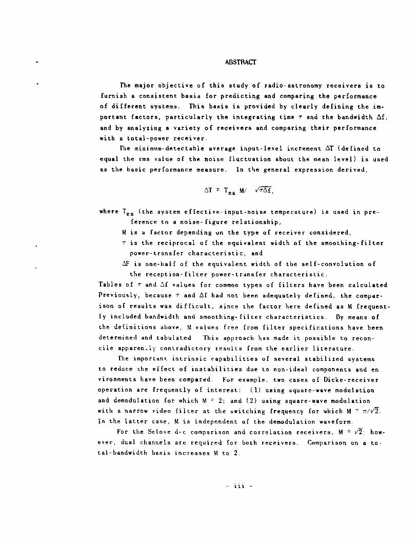
ABSTRACT

The major objective of this study of radio-astronomy receivers is to

furnish a consistent basis for predicting and comparing the performance

of different systems. This basis is provided by clearly defining the im-

portant factors, particularly the integrating time r and the bandwidth 6f,

and by analyzing a variety of receivers and comparing their performance

with a total-power receiver.

rhe minimum-detectable average input-level increment IT (defined to

equal the rms value of the noise fluctuation about the mean level) is used

as the basic performance measure. In the general expression derived,

AT = Tes M/ V-Af ,

where Tes (the system effective-input-noise temperature) is used in pre-

ference to a noise-figure relationship,

M is a factor depending on the type of receiver considered,

'r is the reciprocal of the equivalent width of the smoothing-filter

power-transfer characteristic, and

,F is one-half of the equivalent width of the self-convolution of

the reception-filter power-transfer characteristic.

Tables of r and Af values for common types of filters have been calculated

Previously, because r and Af had not been adequately defined, the compar-

ison of results was difficult, since the factor here defined as M frequent-

ly included bandwidth and smoothing-filter characteristics. By means of

the definitions above, M values free from filter specifications have been

determined and tabulated This approach has made it possible to recon-

cile apparen,.'y contradictory results from the earlier literature.

The important intrinsic capabilities of several stabilized systems

to reduce the effect of instabilities due to non-ideal components and en

vironments have been compared. For example, two cases of Dicke-receiver

operation are frequently of interest: (1) using square-wave modulation

and demodulation for which M = 2; and (2) using square-wave modulation

with a narrow video filter at the switching frequency for which M = 7/v'.

In the latter case, M is independent of the demodulation waveform.

For the Selove d-c comparison and correlation receivers, M = V/2; how-

ever, dual channels are required for both receivers. Comparison on a to-

tal-bandwidth basis increases M to 2.

-. iii -

A comprehensive study of Byle and Vonberg's null-balancing receiver,

which is generally insensitive to instabilities, has shown that its AT

value is equal to that of a Dicke receiver, provided the integrating time

for the null-balancing receiver includes an over-all value considering

the effect of the servo loop. The analysis also showed that a particular

sensitivity to loop-gain stability exists in the following sense. Signals

passing through the receiver suffer time delays that must be allowed for

in data reduction. The fractional error in delay correction is directly

related to the fractional error in loop gain and is independent of the

servo-transfer function of the receiver.

A study of the automatic-gain-control (AGC) system for a total-power

receiver and a modulated pilot-signal receiver showed that, when applied

to a total-power receiver, AGC is useful only when d-c output levels are

not needed.

The modulated pilot-signal system is shown to be theoretically capable

of achieving M values at least equal to 2 when large integrating times

are used in the AGC loop. In contrast to the Dicke receiver, stabilization

against gain changes is independent of the signal level for the modulated

pilot-signal receiver.

The concepts developed in this study have been used to analyze and

evaluate the performance of the Stanford microwave spectroheliograph re-

ceiver, which is described in detail, and to establish the relationship

of the instrument to its antenna and its observational requirements.

- iv -

CWNTENTS

Page

I. Introduction ..... ...................... I

I. Basic Receiver Considerations . .......... 4A. General Receiver Requirements . ............ 4B. The Basic Measurement -- Power Level .... .......... 5C Minimum Detectable Signal ........ ................ 5

1. Definition . ................... 52 Ideal vs. Practical Evaluation ...... ............ 6

1) An Elemental Receiver ......... .................. 61. Description . . . ................ . 62. Analysis . . . . . . . . . . . . . . . . . . . . ... 93. Definitions of Fundamental Parameters .. ........ . 114. Parameter Values for Typical Filters .. ......... ... 12

E. Noise Temperature Concept. .............. 15F. Effective Input-Noise Temperature ............ 17G. Detector Considerations .... ................ 19It. Stability Discussion ...... ................. . 19

III. Total-Power Receivers and Stabilization .. .......... 24A. Characteristics of Total Power Receivers ........ 24

1. Minimum Detectable Signal ..... .............. . 242. Practical Limitations ...... ................ . 24

B Calibration Procedures ...... ................. . 24I. Astronomical Sources ............... 252. Temperature-Controlled Sources ... ............ ... 253 Gas-Discharge Noise Generators ... .......... . 254. Diode Noise Generators ................ 265. Recalil'ration .................... 26

C. Extreme Gain Stability Requirements ........... 26D. Types of Stabilization .............. ..... 27

1. Zero-Point StaLilization . . ........... .28

2. Two-Point Stabilization ..... ............... . 31

IV More-Complex Receivers . . ................ 39A Stabilized Receivers with Unmodulated Signal . ...... . 39

I. Selove-Type Receivers .... ................ 392 Correlation-Type Receivers .... .............. ... 42

B Stabilized Receivers with Modulated Signals ........ . 51I. Introduction . . . . . . . . . .. . . . 512 Dicke Type Receivers ............. 51

C. Receivers with Servo Stabilization .......... 581. Introduction .... ................. 582. Automatic Gain Control Theory ........ 593 Pilot Signal Receivers ............. . 614. Other AGC Systems ......... 71

v -

CONTENTS (Cont'd)

Page

V. Ryle and Vonberg Type Receivers .... ............. . 73A. General Description ...... ................... ... 73

I. Controllable Reference Sources ... ............ ... 732 Error Voltage Amplifiers ..... ............... ... 753. Comparison Devices ...... .................. ... 76

B. Noise Analysis . . . . . . . . . . . . . . . . . . .. . 76C. Dynamic Behavior ........ .................... . 78D. Limitations ... ....................... 81E. Supplementary Smoothing Filters .... ............. ... 85

VI. Stanford Microwave Spectroheliograph deceiver . ....... . 86A. General Requirements ................. 86

1. Bandwidth and Beamwidth Relationship ........... . 862. The Temporal Response of the Receiver .. ........ . 893. Accuracy ........ ... ................... . 89

B. Description of the Receiver ..... ............... ... 921. General ........ ..................... 922. Input Circuitry ....... ................... . 943. B-F and I-F Sections ...... ................. ... 964 Detector and Low-Frequency Section ... .......... . 1005. Demodulation and Output Sections ... ........... ... 1016. Auxiliary Apparatus ...... ................. . 105

C Characteristics and Performance . . .......... 106I. Critical Features ....... .................. . 1062 Minimum Detectable Signal ................. . 108

D. Sample Records ........ .................... . 1081. Fan-Beam Solar Record ...... ................ . 1082. Pencil Beam Solar Record . . . ............ 1093. Weak Source Record ...... ................. . 109

VII. Conclusions . . . . . . . ... ............. 111A. Summary . ....................... illB. Comparative Results ...... .................. . 113C. Suggested Further Study ...... ................. ... 116

Appendix A. Useful Belations|-ips ..... ............... . 118

Appendix B. Analysis of a Correlation Receiver .. ........ . 120

Appendix C Detailed Analysis of the Modulated Receiver .... 124

Appendix 1). Proof of Theorem on Time Displacements Due tosmoothing ........ ..................... ... 132

Appendix E. Details of the Varactor Diode Shorting Section 134

. vi -

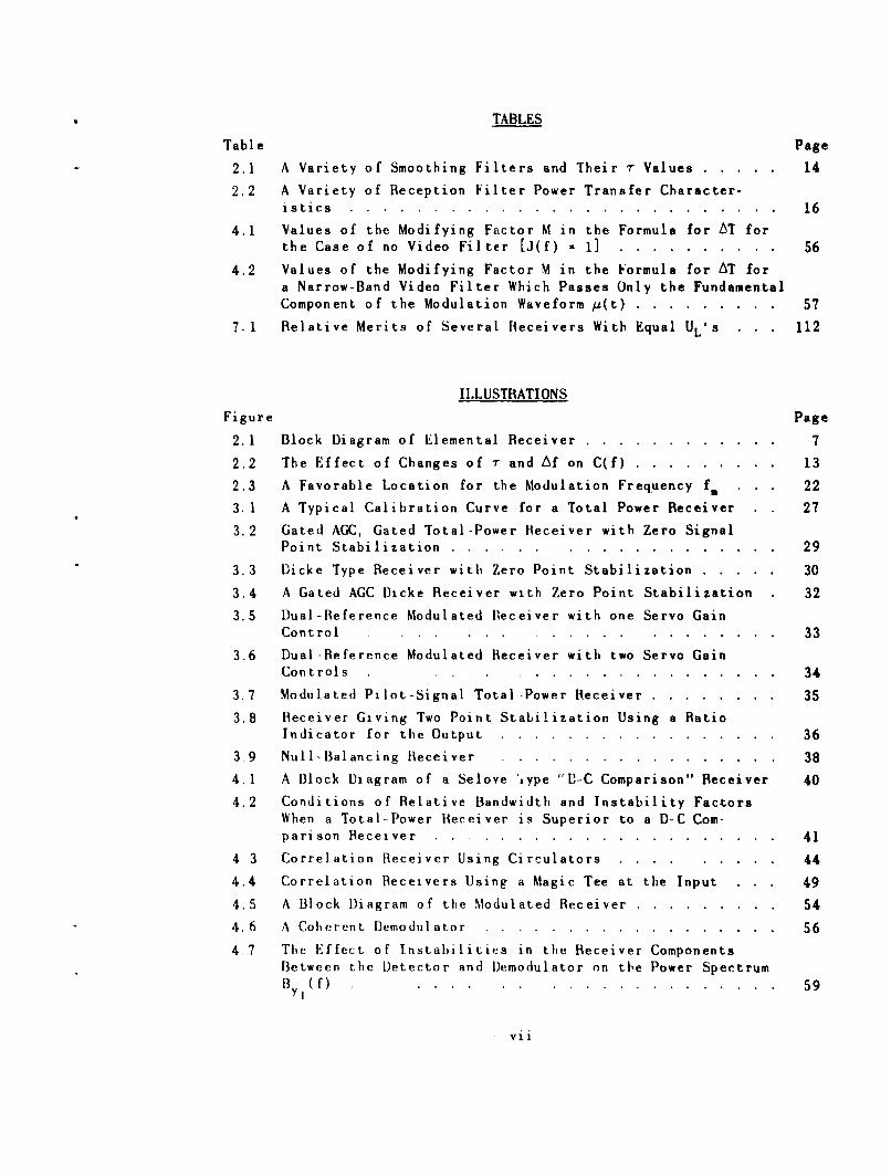
TABLES

Table Page

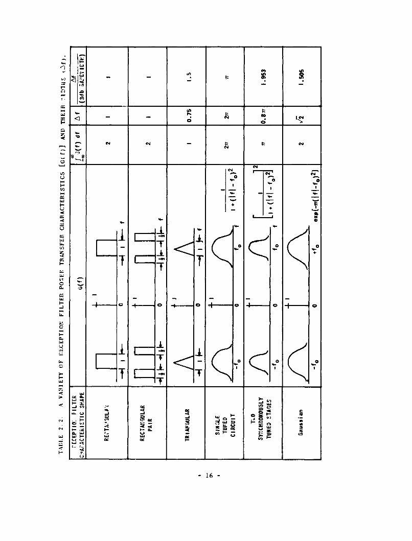
2.1 A Variety of Smoothing Filters and Their r Values ..... . 14

2.2 A Variety of Reception Filter Power Transfer Character-istics .......... .......................... . 16

4.1 Values of the Modifying Factor M in the Formula for AT forthe Case of no Video Filter [J(f) - 1]. ..... .......... 56

4.2 Values of the Modifying Factor M in the Formula for AT fora Narrow-Band Video Filter Which Passes Only the FundamentalComponent of the Modulation Waveform p(t) .. ......... ... 57

7. 1 Relative Merits of Several Receivers With Equal UL's . . . 112

ILLUSTRATIONS

Figure Page

2.1 Block Diagram of Elemental Receiver ...... ............ 7

2.2 The Effect of Changes of r and Af on C(f) .. ......... ... 13

2.3 A Favorable Location for the Modulation Frequency f. 22

3. 1 A Typical Calibration Curve for a Total Power Receiver 27

3.2 Gated AGC, Gated Total-Power Receiver with Zero SignalPoint Stabilization ..... . ................... . 29

3.3 Dicke Type Receiver with Zero Point Stabilization ..... .. 30

3.4 A Gated AGC Dicke Receiver with Zero Point Stabilization 32

3.5 Dual-Reference Modulated Receiver with one Servo GainControl . . . . . ................ . 33

3.6 Dual-Reference Modulated Receiver with two Servo GainControls .... ..................... 34

3.7 Modulated Pilot-Signal Total -Power Receiver .......... ... 35

3.8 Receiver Giving Two Point Stabilization Using a RatioIndicator for the Output ...... ................. . 36

3.9 Null-Balancing Receiver ...... ................. . 38

4.1 A Block Diagram of a Selove ',ype "-C Comparison" Receiver 40

4.2 Conditions of Relative Bandwidth and Instability FactorsWhen a Total-Power Receiver is Superior to a D-C Com-parison Receiver . . . . . . . . . . . . . . . . . . . . . . 41

4 3 Correlation Receiver Using Circulators . . . ....... 44

4.4 Correlation Receivers Using a Magic Tee at the Input . . . 49

4.5 A Block Diagram of the Modulated Receiver .. ......... ... 54

4.6 A Coherent Demodulator ....... .................. . 56

4.7 The Effect of Instabilities in the Receiver ComponentsBetween the Detector and Demodulator on the Power SpectrumB (f) .... .............. 59

vii

ILLUSTRATIONS (Cont' d)

r'igure Page

4.8 Block Diagram of an AGC Loop in a Total Power Receiver 60

4.9 Assymptotic.-Frequency-Response Curves for the ReceiverWith AGC ......... ......................... ... 62

4.10 Requirements on Filter Break Frequencies ........... ... 63

4.11 Block Diagram for a Modulated Pilot-Signal-StabilizedReceiver ......... ......................... ... 64

4.12 Representation of the AGC Loop in the Modulated Pilot-Signal Receiver ....... ..................... .. 66

4.13 Ratio of Pilot-Signal to Signal Integrating Times as aFunction of M Factor for a Pilot-Signal AGC Receiver 69

4.14 Normalized Asymptotic Response to Instabilities of aModulated Pilot Signal Receiver ... ............. .. 70

5.1 Simplifi-d Block Diagram for a Ryle and Vonberg TypeNoise-Balancing Receiver ..... ................. ... 74

5.2 Simple Servo-System Block Diagram ... ............ .. 80

5.3 Spectra and Time Functions Showing the two SmoothingOperations Occurring During the Observation of a Dfiscrete

Source .......... .......................... .. 83

6.1 The Relative Beam Broadening .... ............... ... 88

6.2 Half-Power Beam Width for a Single Array vs. Order ofInterference ........ ....................... ... 90

6 3 Half-Power Beam Widths for the Cross Antenna vs. Order ofInterference ........ ....................... ... 91

6.4 Block Diagram of the Cross Receiver .. ........... . 93

6 5 Diagram of the Phase Switch for Cross Operation .... 95

6 6 Variable Phase Length Shorts for the Phase Switch .... 97

6.7 Addition to the Phase Switch Which Produces a Double-Throw

Microwave Switch . ............ . 98

6.8 Block Diagram of the R-F and I-F Sections of the Receiver 99

6 9 Power Besponse Curve for the Complete Receiver . . . 100

6 10 Block Diagram of the Receiver from I-F Attenuator Through

the Coherent Demodulator . .. ........ 102

6 11 Coherent Demodulator ...... . . 103

6.12 Smoothing Filter Switching and Integrating Times I 1 104

6.13 Cathode Follower Output Circuit ......... . 105

6 14 Sample Solar Record Showing Fan-Beam Scans . 109

6.15 A Sample Solar Record Showing Pencil-Beam Scans . . 110

6.16 A Sample Record Showing a Fan Beam Scan of the Moon 110

- viii -

SYMBOLS

c output voltage of a servo system; velocity of light

e error voltage of a servo system

f frequency

h impulse response

k Boltzman's constant

1 junction load voltage

Fr order of interference

n noise voltage

p strength

q angle measured from a plane perpendicular to an antenna array

r input voltage of a servo system

s complex frequency

t time

v voltage

w equivalent width

x detector-input voltage

y detector-output voltage

z meter deflection at output of receiver

A,B,C,D power spectral densities (PSD)

F noise figure

G,H power-transfer characteristics of reception filter, smoothingfilter

I fractional rms variation of the output due to instabilities

J power-transfer characteristic of video filter

K coefficients

L reference level

M factor to account for mode of receiver operation

N noise power at receiver output

P antenna response (field)

R resistance

S signal power

T temperature (oK)

U uncertainty figure

Y voltage transform of detector output <y>

m voltage from the equivalent moiulator

s spatial frequency

t time-displacement variable

- ix -

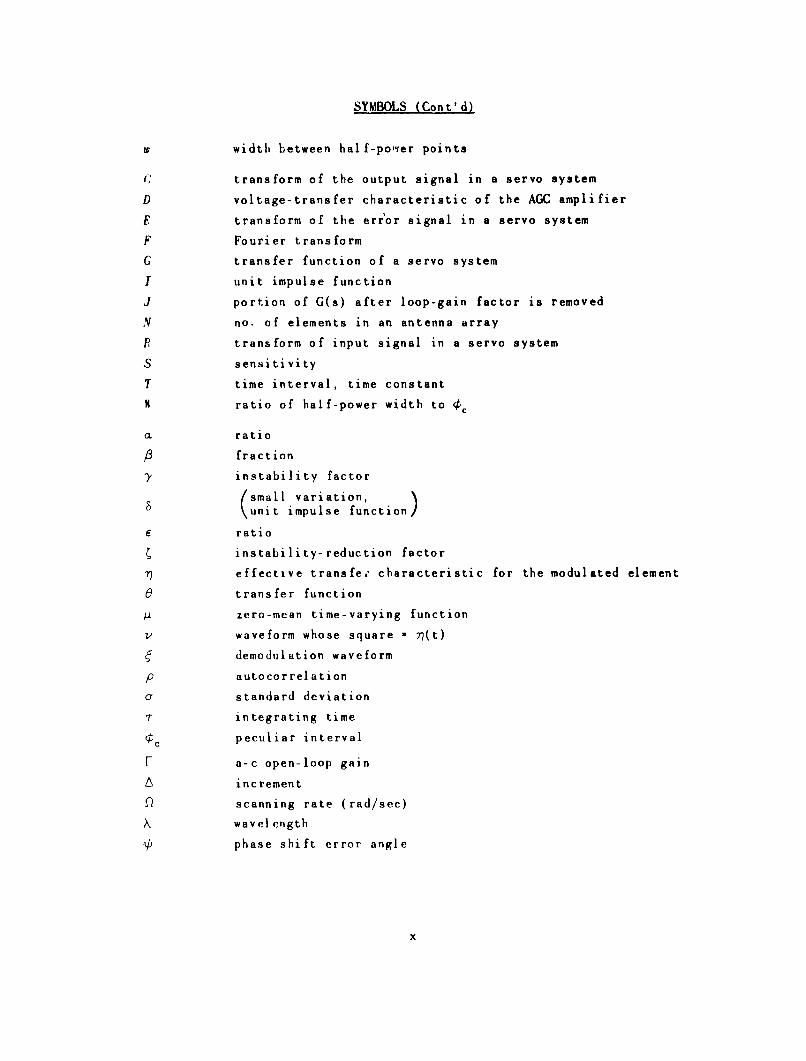
SYMBOLS (Cont'd)

W width between hal f-poier points

C transform of the output signal in a servo system

D voltage-transfer characteristic of the AGC amplifier

E transform of the err'or signal in a servo system

F Fourier transform

G transfer function of a servo system

I unit impulse function

J portion of G(s) after loop-gain factor is removed

N no. of elements in an antenna array

P transform of input signal in a servo system

S sensitivity

T time interval, time constant

9 ratio of half-power width to

a ratio

18 fraction

^Y instability factor

small variation, )unit impulse function

E ratio

instability-reduction factor

71 effective transfee characteristic for the modulated element

0 transfer function

JU zero-mean time-varying function

v waveform whose square - 7?(t)

demodulation waveform

p autocorrelation

a standard deviation

Tintegrating time

¢tc peculiar interval

F a-c open-loop gain

A increment

scanning rate (rad/sec)

wavelength

phase shift error angle

x

SYMBOLS (Cont'd)

Subscripts

a AGC loop

b break

c continuous

d noise diode

* effective input

f ferrite attenuator

g loop gain of servo

h impulse response

i ,j indices

I low-frequency cut off

M modulation

n number

o center frequency of receiver response

p pilot

q angle measured from a plane perpendicular to an antennaarray

r receiver

a system

u unwanted source

v voltage

* wanted source

x before detection

y after detection

A acceleration

C circulator

D demodulator

F video tilter

G,H power-transfer characteristics of reception filter,smoothing filter

I instability

J hybrid-tee junction

L level

M motor

P position

S signal power

T total

V velocity

- xi -

SYMBOLS (Cont'd)

Subscripts

a ampli fier

comparison

h highest

p pilot

s signal

t tuned filter

7)modulated

K index no.

A'modulated waveform

index for error coefficient

demodulated waveform

feedback

- xii -

ACKNOWLEDGMENT

I wish to express my gratitude to Professor B. N. Bracewell for his

guidance and supervision and to Professor G. Swarup for many helpful

comments. Mr. C. L. Seeger deserves special thanks for his inspiration,

encouragement and support. Thanks also go to Mr. U. D. Cudaback to whom

I am indebted for many valuable discussions as well as assistance during

the development of the receiver. The associations with colleagues and

the staff of the Badioscience Laburatory have been of great value.

I wish to express to my wife, Mary Mae, my never-ending appreciation

for her encouragement and understanding, which carried me through to the

completion of this work.

xlii -

I. INTRODUCTION

A radio-astronomy receiver produces at its output an indication of

the total effective noise power applied to its input. This indication

changes when a signal is present. Whenever a measurement is made, the

signal induced change is compared with changes made by substituted sources

of known noise power. Assuming a perfectly stable receiver we can readily

determine the theoretical accuracy of such a measurement.

It is convenient, in practice, to measure the signal powers in units

of degrees Kelvin by the use and extension of Nyqlist's theorem, which

linearly relates an equivalent temperature with a noise power whenever a

definite frequency band is involved. In this way Dicke [Ref. 1] first

derived the expression,

AT a (Constant) Tes/VT Lf

which relates the rms variation of the receiver output AT to certain

characteristics of the measurement procedure. Here, Tea is the effective

system input-noise temperature in degrees Kelvin; f is the pre-detection,

or high-frequency, bandwidth of the receiving system; and r is the post-

detection integrating, or averaging, time.

Although the above parameters are generally included in some form in

all receiver discussions, the diversity of arrangements arising because

of individual requirements has led to certain difficulties when com.-

paring performance. That is. the parameters are often modified for

special cases and so are not easily generalized. Also, further complexity

is introduced because of special designs that are employed to minimize

practical limitations set by particular component characteristics, es-

pecially in relation to their stability.

In this study explicit, general definitions for the parameters of

bandwidth and integration time are given. They are derived from the analy

sis of an elemental receiver, then modified and expanded to include a widerange of complex receivers

With the advent of masers and p.rametric amplifiers, our knowledge of

the fundamental causes of system noise has increased rapidly until, now,we believc the theory is fairly complete. As a result, the new low-noise

devices approach ever closer to predictable, natural limits [Ref. 2), and

the belief is that the existence of these limits is well established, so

- I

that future developments in amplifying devices will not yield large per-

centage improvements in their effective noise temperature. As a con-

sequence, receiver stability assumes an ever more serious character, since

it is then becoming the major limitation to receiver performance. Insta-

bility increases T in practice just as effectively as does a large in-

crease in system-noise temperature, so that either intrinsic stability

must be improved or the effects of instability must be reduced by the

adoption of special observing procedures. Stabilities of one part in 103

are normal good practice, while 104 is unusual.

Because of imperfections in existing equipment, correlation receivers

and various forms of switched-input receivers have been developed or pro.-

posed. Comparisons of the theoretical capabilities of many of these re-

ceivers differ by factors on the order of 2, root 2 and pi, which, although

small, have considerable economic significance. In this study we provide

useful theoretical comparisons, derived in a consistent manner, which

should be applicable to all radio-astronomy receivers. In a numier of

cases, numerical calculations are presented to illtstrate a practical range

of situations

The 'minimum. detectable mean-input-level increment" is used as the

performance criterion in this work. Although the phrase "minimum detectable

signal" suffices at times, the longer and more exact statement always should

be understood. The basis for this criterion is a simple level measurement

echniques of stabilization may be divided into three categories, de-

pending on methods of treating the signal in the receiver. The signal

may be

I unmodulated,

2 modulated, or

3 a null balanced or error signal.

he analysis of correlation and Dicke-type receivers in Chapter IV uses

examples from categories I and 2. The null-balancing receiver is discussed

in Chapter V Whereas the naterial in Chapter IV is mainly an extension

and codi fication of previous work, but in a much more general form, the

analysis of tie null balancing receiver is believed to be a new contri-

but.on to the field The application of servo control or automatic gain

control (AGC) to radio-astronomy receivers is treated in detail, and many

interesting aspects are presented for which there has been no prior dis-

cII SSio nl

2-

A specialized receiver developed for use with the Stanford Microwave

Spectroheliograph is described in Chapter VI. The concepts developed in

earlier chapters are used in the discussion of the specifications and the

performance of this receiver. Also the effects of restrictions placed on

receiver design because of the antenna system and the anticipated ob-

serving programs are considered.

Finally, it is pointed out that the successful development of a high-

performance receiver for sensitive radio-astronomical investigations is

an art, as much as it appears to be a matter of straightforward engineer-

ing.

3-

II. BASIC RECEIVER CONSIDERATIONS

A. GENERAL RECEIVER REQUIREMENTS

In radio astronomy, receivers are often designed to operate with a

particular antenna to form a radiotelescope, which is frequently designed

for, or is inherently capable of performing, only a limited variety of

measurements in a satisfactory manner. Because of these facts, it is nec-

essary to compare receivers with care, concentrating on those characteristics

which are basic to all systems.

Here we consider the radiotelescope as a transdicer acting between

incident electromagnetic energy and a record of one or more of the charac-

teristics of this radiation. We can list a general set of requirements

for this transditcer as follows:

1. It must sense a region of space or sky with a particular antennapattern

2. It must use a particular portion of the radio-frequency (r-f)spectrum.

3. The time-varying aspects of the observation must be handled satis-factori ly

4 The record produced should be, as much as possible, only a measureof the desired characteristic.

5. The record should have the requisite range and accuracy

In general, and as a practical matter, these items are interrelated.

For instance, items I and 2 must be considered together since the antenna

pattern is a function of frequency although the receiver chiefly determines

the frequency reception band.

Now we can assume that the over-all design provides for the measure-

ment of the desired characteristics and we Lan then list some general

receiver specifications as follows:

1. Spectral response, i.e., operating frequency, bandshape, and band-width

2 Temperal response, i.e., ability to follow expected changes of theinput with time

3 lange and accuracy, i.e , least to greatest value of the measuredvariables with specified limits of error

The effect of design parameters on item 3, particularly as regards

the least values of the desired measures, is of great interest.

4

Receivers in use up to this time have exhibited wide ranges in these

specifications. Nearly the whole spectrum made available through current

radio technology has been used. The values of signal strength, in terms

of temperature, range from a few hundredths of a degree to more than106 OK. Bandwidths vary from a few kilocycles to hundreds of megacycles.

Measurements made include, for example, the detection of weak sources with

measurements of their strengths and positions, source-brightness distri-

butions, spectral variations and temporal variations of sources, and so

forth. The objectives of radio astronomy cover a wide field.

B. THE BASIC MEASUREMENT POWER LEVEL

Underlying the majority of measurements with radiotelescopes is a

requirement for the determination of relative power at low levels. In

the detection of sources, the problem often is to determine that minimum

change in power level, as indicated by the receiver, which can be cor-

rectly ascribed to a source, and not to "faults" in the receiver. By

throughly discussing just this simple measurement.-the determination of

the power level or strength of a constant source- we are well prepared

to understand more complex measurements. The capabilities of a receiver

with regard to this simple measurement of power level will be discussed

below and a general expression will be given which specifies a performance

figure, or figure of merit.

C MINIMUM DETECTABLE SIGNAL

The detection of a simple change in input power level depends, in

practice, on more than just the properties of the radiotelescope or the

receiver alone. llowever, for our purposes, considerations other than

those relating to the receiver alone are not included, since we wish to

establish only the properties of the receiver.

1. D)efinition

In order to be removed from any characteristics of the operator,

we establish a criterion of detectability on the basis of a convenient

mathematical definition. This criterion may be stated as follows: when

at tie output meter the mean deflection increment corresponding to a sig-

nal increase equals the standard deviation of the fluctuations about the

mean deflection, this mean deflection increment is said to be detectable

In pratice, (f course, experience often wisely dictates the use of a several-times

1arg'r increment-5-

2. Ideal vs. Practical Evaluation

The idealized design of the receiver sets forth the necessary de-

tails from which a performance figure for detectability can be calculated.

The practical receiver will have instabilities of gain, bandwidth, and

effective-input-noise temperature which will degrade the ideal perform-

ance by some factor.

D. AN ELEMENTAL RECEIVER

The quantity to be measured by the receiver is the strength of a

source of energy having an essentially uniform power-spectral density

(PSD) over the observing range of frequencies. Furthermore, as is fre-

quently the case, the source is assumed to produce an ideal fluctuating

voltage, i e., one with a stationary gaussian amplitude distribution about

a zero mean value. Within the receiver, the energy from a particular

source undergoes alterations and ultimately produces a deflection on the

output meter. In general the meter deflection consists of unwanted com-

ponents, such as receiver noise and zero offset, in addition to the com-

ponent due to signal from the source to be measured If the receiver is

calibrated* to yield a unit mean deflection for a unit mean-input-level

increment, deflection and incremental input level can be equated. This

stratagem allows us, for an idealized, stable receiver, to dispense with

discussing receiver gain, which, although of practical importance, does

not affect intrinsically the power-level-detection performance

The ratio of the detectable mean-deflection increment to the mean meter

deflection may be considered constant for a given elemental-receiver de-

sign, as will be shown, so that this ratio is a measure of performance.

The ,ninimum detectable input-level increment will therefore depend on the

unwanted source strengths, referred to the receiver input, which for the

elemental receiver determine the mean output-meter def. ection at zero

signal.

1. IUescription

The elemental receiver analyzed below is shown in block diagram

form in Fig 2.1. The receiver responds both to the signal and to an

Calibration is assumed possible with an accuracy much greater than the accuracy ofthe measurements to be made. This assumption keeps practical details such as needlewidth, dead zone, ink-line width, and scale reading in general from contributing tothe detectability criterion.

6-

'a-

II~'4- 0

'a-N

S0

lii'4..'

m ~ 0 -

me-m

I-

Is! U~2lb

me- C

I- -

me.. -me.- .~ K C

0

WI'.

'a..

-7-

unwanted source of energy at its input. The latter input is equivalent,

with regard to meter deflection, to all actual unwanted contributions

distributed throughout the receiver, such as those associated with trans-

mission loss, amplifier noise, and frequency-conversion loss. We shall

consider only inputs having uniform power per unit frequency interval

All elements except the final detector are assumed to be linear.

The reception filter is equivalent to the combined effect of all

the frequency-sensitive elements in the system, such as the antennas,

transmission lines, r-f and i-f amplifiers, mixers, and any selective

filters that may be used. Thus the portion of the spectrum from which

energy can be received is defined by d power-transfer characteristic

G(f), which is the ratio of the output to input PSO's of the reception

filter at all points in the spectrum. Since we are dealing here only

with inputs having uniform PSD's, the PSD of the reception-filter output,

and of the detector input, will be

A(f) - (p +p0 ) G(f)

where p, is the strength of the source to be measured and pu is the

strength of the unwanted source at the input measured in units of w/cps.

The spread of A(f) is assumed to be small compared with the mean frequency.

The voltage x(t) at the detector input has a gaussian amplitude

distribution with zero mean and PSD A(f). The exact voltage as a func-

tion of time x(t) is actually not known, of course, but its statistical

properties are, and they are used in the detector analysis and after.

Similar statemcits hold for other quantities such as y(t) and z(t), used

later.

For the elemental receiver, an ideal square-law detector circuit

is employed with one ohm impedance levels so that

y(t) - x2(t)

and the mean output voltage <y> equals the power at the detector input

thus

'<Y> a <X2>

The sharp brackets indicate the following averaging operation,

- 8-

T< - lim I. y(t) dt.

Fluctuations of y(t) about the mean are governed by the continuous por-

tion of the detector output PSD B(f).

After detection, the fluctuations about the mean are reduced by

a smoothing filter with power-transfer characteristic H(f). A typical

smoothing filter might be a single-section, lowpass HC circuit. The

smoothed output voltage is then displayed as a meter deflection. For

generality we include any selective effects (usually further smoothing)of the meter in H(f) by taking z(t) to be the true meter deflection.

2. Analysis

As stated above, the PSi) A(f) of the detector input voltage x(t)

is

A (M) (p. + pu) G(f).

The total power at the detector input is, using Eq. (A.4)*

J A (f) df m px(0) = <x2>. O

where px(0) is the central ordinate of the autocorrelation function of

the detector input voltage. Now, using the relationship of Eq. (A.8)

for the PSD of the detector output voltage y(t),

B(f) - 2 f p2 exp(-j2lvfT)dr + px2(0) (f)

- 2[A(f)* A(f)] + p2(0) 8(f)

AEAppendix A, Eq. (A-4).

-9

At the output of the receiver, the PSD of the meter deflection z(t) is

C(f) H(f) B(f)

S211(f) [A( f) * A( f)] +lI(f) p2(0) 8(f).

Since z(t) and y(t) arc related by the voltage response of the smoothing

filter, it follows that

'<Z> - '<y> • VH(0) p1 (O).

We can now form an expression for the detectable mean-deflection

incrementAz, which we defined earlier to be equal to the rms variation

about the mean of the meter deflection z(t).

Az • <z2> - <z>2

I C(f)df- H(0) p.2(0)

This becomes

z- 2 f 1H(F) [A(f)" A(f)] df- C

Generally, the smoothing-filter power-transfer characteristic

will be only a few cycles per second wide while the PSD B(f) will have

widths on the order of megacycles per second. When this is true tA-A)

can be assumed constant over the total effective width of H(f) so that

cc M

f M1(f) [A*A] df - [A-Al J H(f) df. (1)

With this assumption, the expression for the ratio of detectable mean

deflection increment to the mean deflection will be

- 10 -

6z/<z> . 2[A*AS 0 j H(f) df/p2(0) H(O)-GO

Using the equivalent width w1 and expressing p2(0) in terms of A(f),

the equation above becomes

Az/<z> /2(A-A]I 0 wH/ A(f) df (2)

Using Eqs. (A.4) and (A.5),

A(f) df 2 p2(0) f [A*A) df.

When A(f) is replaced in (2) with (pw +pu) G(f), terms in (p.+pu)vanish,

and when equivalent width WG.G is used it is now evident that

L\z/< z> 2w 4 2l/WG-G

3. Definitions of Fundamental Parameters

If we define an integrating time -r and a bandwidth f as follows,

M

1 l/w, - 11(0)/ f Milf) df (3)-C

Af u WG.G/2 f [G*G] df/2[G*G] 0 (4)

we can express the ratio

/ tz/<z> ( l/V/--f ' (5)

See Appendix A, Eq (A.6)

-11

Henceforth this ratio will be called the level-uncertainty figure. For

the elemental receiver, UL equals the minimum- detectable iucrement of

mean meter deflection divided by the mean meter deflection. For generality,

UL, expressed in terms of the input, equals the fractional uncertainty of

measurement of input level, or the ratio of minimum-detectable mean input-

level increment to the mean input level. As will be discussed below,

many receivers operate with a suppression of the zero-signal mean meterdeflection. Then the mean input level is no longer directly related to

the mean meter deflection, so that UL has meaning in terms of input levels

only.

The form UL describes the instrument's capabilities with respectto indicating changes in input level. In order to evaluate UL it is

necessary to be able to assign values of r and Af to the receiver. Since

these parameters have been explicitly defined in Eqs. (3) and (4) their

values and the resulting value for UL can be determined.

To understand better the roles of r and Af, consider the PSD C(f)

at the output meter and note the effect of changes in 'r and f. Figure2 .2(a) shows a typical C(f). Note the following points: there is an

impulse function at zero frequency, indicated by a vertical arrow, of

strength equal to <z> 2 ; the central ordinate of the continuous portion

of the function is designated Cc(O); and the shading in Fig. 2.2 shows

the area under the continuous portion, Cc(f). The smoothing filter

limits the extent in frequency of Co(f). Since the area under C,(f)

equals the square of the detectable mean deflection increment, we see

that, by narrowing 1l(f), and, hence, CC(f), the detectable mean de-

flection increment is reduced. Figure 2 2(b) shows the effect of narrow-

ing 11(f), which is equivalent to increasing r.

4 Parameter Values for Typical Filters

In Table 2.1, w11 and r are listed for a variety of smoothing fil-

ters in terms of filter specifications. Many circuit configurations can

yield the same -, so that, for simple measurements of input-level incre-

ments, as discussed here, the choice of filter is a matter of convenience,

but with tOe restriction that its response be limited to a region of the

spectrum where its input power spectral density can be assumed constant.

[See Eq. (1)]

The reception filter determines the amplitude of Cc(O) in relation

to <z> 2 The following relationships show that Af implicitly contains

this information.

- 12 -

c(f)2

e(f) f(f)

< z >2 (a) < 1 >2

INCREASE

f INCIEASE Af

0 f T

(b) (c)

FIG. 2.2 EFFECT OF CHANGES OF 'r AND Af ON C(f). IN (a) A COMPARISON SITUATION IS

SHOWN WIH1 (b) SHOWING THE EFFECT OF INCREASING T AND (c) SHOWING THE EFFECT OF

INCREASING Af. THE SCALE OF (c) IS NORMALIZED TO HAVE THE SAME AMPLITUDE F)R< 2 >2 AS IN (a).

- 13 -

Ni Q

040

- -~ - 4.

49

-IV,

(4

4C

C144

.4.4

I-L

W 0 0 0i 4

c4 - 0CA

41

0S S

f [G*GI df f CA*A] df6f . WG*G . -w a -D

2 2(G*G] I 2(A*A]I

0

•<Z > 2

p(O) __

Co(0)

Figure 2.2(c) shows the effect of an increased Af on C(f) over the con-dition of Fig. 2.2(a).

The equivalent width, defined above as a self-convolution of theeven function G(f), is suitable for describing reception-filter responses

for which the usual concepts of bandwidth break down or are difficult toapply. It will cover, for instance, bands with notches or peaks in their

response and so may not have unequivocal center frequencies or maximumresponses. Values of Af for a few reception-filter responses are listed

in Table 2.2.

The level-uncertainty figure UL was introduced as a parameter to

indicate the measuring ability of the combined reception and smoothing

filters when fully utilized. Since techniques for improving other char-

acteristics of a receiver sometimes result in reduced utilization of thefilters, the uncertainty of measurement for a complete receiver may in-

volve a modifying factor M applied to UL.

Before covering various receiving systems and their associated Mvalues, a discussion of some of the practical aspects of receivers that

affect UL will be given in the next sections.

E. NOISE-TEMPERATUBE ONCEPT

The total power at the detector input can be divided by the powergain of the receiver up to that point in order to refer the power to the

receiver input. When this input noise power is equated to the thermal

noise power from a matched termination at the input to the receiver, therequired temperature of the terminatinn becomes a convenient measure of

the effective input noise power.

15

-) <14

ca- I

<1j -.C

I-- C- cr c Q

toa

4A- A NA N -

law88

- 16

The source strengths p, and Pu can be described by an effective

noise temperature by being equated to the strength of a thermal source

at some teperature T by the relation

p w kT

w/cps when they have constant power per unit frequency interval. This

is a common and highly precise assumption. For incoherent sources, the

strengths of two or more sources add to give the total strength and like-

wise their effective noise temperatures add.

Input noise temperature will be used almost exclusiveily in dis.

cussing signals and unwanted sources with their strengths having been

referred to t'le receiver input.

F EFFECTIVE INPUT..NOISE TEMPERATURE

An elemental receiver includes unwanted sources of energy that con-

tribute to the mean meter deflection. When the signal source strength

is reduced to zero, there remains a mean meter deflection which can be

ascribed to an equivalent unwanted source strength Pu at the receiver

input. This equivalent receiver input and the level-uncertainty figure

determine the minimum detectable input level increment for the receiver.

If we express this increment and the equivalent unwanted source strength

in terms of input-noise temperatures, the relation of Eq. (5) becomes

ZAT - U

es

where "E is tLe minimum detectable input temperature increment and Tea

is the effective system input noise temperature. In radio astronomy

the measurement of signal strength is limited by the total effective

noise power present. Expressed in terms of the receiver input as T

it becomes an important parameter which is used to represent the tem-

perature of an equivalent source of noise including receiver noise,

transmission -line. loss noise and all sources of unwanted noise in the

antenna reception pattern. The inclusion of this last unwanted noise

results from a broad use of the system concept.

If we were to use an "average noise factor" [Ref 3] to describe the

system and determine AT, we would be limited by the accepted defi'iition

17 -

of the term. First, F is defined in terms of a standard temperature for

the signal. source. Since signal source temperature is what we are trying

to measure the introduction of a standard temperature seems inappropriate

in order to describe receiver performance. However, if we use the cor-

responding term "average effective input-noise temper-ature" TO we are

free from any standard temperature requirement. T. is "the irput ter--

mination noise temperature which, when the input termination is con-

nected to a noise-free equivalent of the transducer, would result in the

same output noise power as that of the actual transducer connected to a

noise-free input termination... (and] T. a 290 (F-1)" [Ref. 3]. The

symbol Tee* is a special use of this concept in that the transducer must

be extended to include not only the receiver and antenna but the back-

ground radiation upon which the signal is superimposed, and averaged

over the reception band. We can then paraphrase the above definition,

" Tes is the avera ... the actual transducer "connected" to a signal-

free region of the sky." (The underlined portions are changed )

A second reason for avoiding V is that radiometer usage of heterodyne

systems make the definition of F inappropriate since a different re-

lation between it and Tea must be used for each case. For instance, in

a tuned r-f receiver

Tea" 290 (F - 1)

and for the usual heterodyne case when both the image and signal bands

contribute equally to signal and unwanted output components

Tea - 290 [(F/2) -1)]

For minimum-detectable input-temperature increments, given a con-

dition of signal level, which we designate AT(T) where T is signal.input

temperature, the mean input level will include a contribution from the

signal as well as from unwanted sources. Then

We drop the bar over Tea for convenience, but Tes is an average.

- 18-

?T(T) - M T.. UL

where T' is the effective input temperature, including effective signal

temperature. For the elemental receiver

T's 0 Tes + 1.

G. DETECTOR CONSIDERATIONS

Although the detection process can be accomplished with different

types of detectors, the square-law detector was chosen for the above

analysis, a choice which, for small signals, results in no loss of general-

ity. Strum [Ref 4] points out that AT must be increased only 1 05 if a

linear detector is used and that the behavior of other general-law de-

tectors approaches that of the square-law detector for small signals.

Lampard [Ref. 51 and Kelly, Lyons, and Root [Ref. 63 have shown the

optimum detector law to be the square law for a simple change in level

measurement.

H. STABILITY DISCUSSION

In the analysis of the elemental receiver, complete stability, in the

sense of constancy of the receiver characteristics was assumed (although

non-ideal operation as far as unwanted noise sources was considered), but,in fact, the fluctuating component of the meter deflection is dependent

on the stability of the receiver. All departures from a stable operating

condition contribute an addition to the meter-deflection power spectrum

In general, the additional spectral components will have these character-

istics:

1. No d-c component (by definition)

2. Concentration of spectral density around d-c

3. Rapidly decreasing strength with increase of frequency4. Possible peaks or line spectra associated with power-source har-

monics or microphonics

The result of the output variations due to instability will be to

increase AT. However, depending on the instability spectrum compared to

that of the signal, the result can be more or less deleterious since, for

signal variations rapid compared to those due to instability, the

- 19 -

detectability of the signal will not be greatly affected. Slow variations

in the output due to such things as gain deterioration are generally re-

ferred to as drifts. When the period of measurement is short, the drift

is quasi-linear and can be removed from the record without serious effect.

As the relative period of measurement increases and the drifts take on

curvature and inflections, they constitute a serious degradation of signal

which is difficult to evaluate. When the variations have taken on the

character of fluctuations they are amenable to inclusion in the minimum

detectable signal expression as follows. The rms value of fluctuations

in the meter deflection referred to the input will be the quadratic sum

of components due to sources and to instabilities.

L +12,AT - T %2

where I is the fractional rms variation due to instability alone. This

expression can be written in the form

AT/T U. 1 + (I/UL)2 a UL Y (6)

where y is t!he instability factor for the receiver.

Three characteristics of a receiver that can produce instabilities

are its gain, equivalent noise temperature, and frequency response. A

change of any of the three will produce a change in meter deflection.

The noise temperature, however, is essentially different, since it does

not directly influence the signal amplitude

One approach to actieving stability is by stabilizing the gain through

an automatic--gain control (AGC) system What is commonly called AGC

,isi.i ly operates to maintai" constant output from the receiver over periods

long compared to signai observing times and does not operate to produce

constant gain Consequently any gain change controlled by this AGC may

in fact be compensating for a change in equivalent noise temperature

This situation results in possible subtle changes in calibration and must

be considered when this AGC is used. A true AGC system is discussed in

Chapter IV, Section C.3.

The answer to difficulties of this type is a mode of operation which

makes the mean meter deflection zero in the absence of signal Dicke

- 20

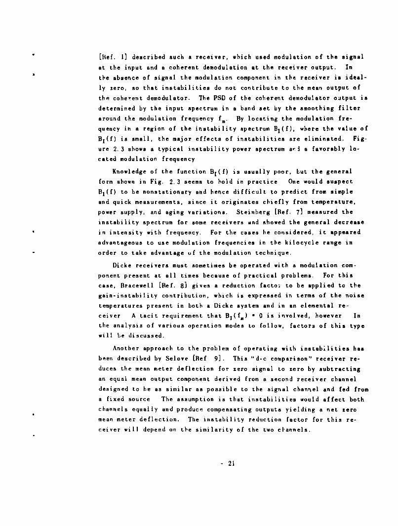
[ef. 1] described such a receiver, which used modulation of the signal

at the input and a coherent demodulation at the receiver output. In

the absence of signal the modulation component in the receiver is ideal-

ly zero, so that instabilities do not contribute to the mean output of

the coherent demodulator. The PSD of the coherent demodulator output is

determined by the input spectrum in a band set by the smoothing filter

around the modulation frequency f.. By locating the modulation fre-

quency in a region of the instability spectrum Bi(f), where the value of

Bi(f) is small, the major effects of instabilities are eliminated. Fig-

ure 2.3 shows a typical instability power spectrum ari a favorably lo-

cated modulation frequency

Knowledge of the function B1 (f) is usually poor, but the general

form shown in Fig. 2.3 seems to hold in practice. One would suspect

BI(f) to be nonstationary and hence difficult to predict from simple

and quick measurements, since it originates chiefly from temperature,

power supply, and aging variations. Steinberg [Ref. 71 measured the

instability spectrum for some receivers and showed the general decrease

in intensity with frequency. For the cases be considered, it appeared

advantageous to use modulation frequencies in the kilocycle range in

order to take advantage uf the modulation technique.

Dicke receivers must sometimes be operated with a modulation com-

ponent present at all times because of practical problems. For this

case, Bracewell (Ref. 81 gives a reduction facto- to be applied to the

gain-instability contribution, which is expressed in terms of the noise

temperatures present in both a Dicke system and in an elemental re-

ceiver A tacit requirement that B1 (f.) - 0 is involved, however In

the analysis of various operation modes to follow, factors of this type

will |be discussed.

Another approach to the problem of operating with instabilities has

been described by Selove (Ref 91. This "d-c comparison" receiver re-

duces the mean meter deflection for zero signal to zero by subtracting

an equal mean output component derived from a second receiver channel

designed to be as similar as possible to the signal channel and fed from

a fixed source The assumption is that instabilities would affect both

channels equally and produce compensating outputs yielding a net zero

mean meter deflection. The instability reduction factor for this re-

ceiver will depend on the similarity of the two cIannels.

21

~0

22-

I.-

.'cn.,

- 22 -

A third approach to the instability problem was analysed by Goldstein

(Refs 10,11]. In this receiver the input signal is impressed on two

channels, which have independent equivalent-receiver-noise sources.

After amplification the outputs of the two channels are multiplied to-

getber. In the absence of signal the output of the multiplier should be

zero. Receivers of this type are also discussed in detail in the follow-

ing chapters.

23 -

III. TOTAL-POWER RECEIVERS AND STABILIZATION

A. CHARACTERISTICS OF TOTAL-POWER RECEIVERS

1. Minimum Detectable Signal

The analysis of the elemental receiver is directly applicable to

a type of receiver usually called a total-power or d-c receiver. In this

receiver we find all the components of the elemental receiver, but with

the gain present in r-f and i-f amplifiers before the detector and in d-c

amplifiers after the detector. The expression for AT of the elemental

receiver is usable with the addition of the instability factor defined in

Eq. (6); thus

AT - Tea UL Y

for the total power receiver.

2. Practical Limitations

The mean meter deflection due to Te, at zero signal, is often

larger than the deflection due to the signal, so that it is common prac-

tice to subtract a fixed d-c level corresponding to the expected mean

meter deflection before impressing the output on the meter. (The quantity

subtracted is often called the "buck-out" or "back-off".) This practice

increases the percentage of full-scale deflection per unit signal but,

of course, also increases the percentage deflection for oatput changes due

to instability in the receiver.

Since the only way to stabilize a total-power receiver is to make

each part more stable than required of the whole receiver, great, and

sometimes impractical, care is required in its design and construction.

A useful receiver of this type designed for observations at meter wave-

lengths, is described by Seeger, Stumpers and van Hurck [Ref. 121.

B. CALIBRATION PHOCEDURES

For a radio-astronomy receiver, convenient scale units for the output

are OK of effective noise temperature at the input. A calibration curve

shows the relationship between input temperature and scale divisions on

the output meter

- 24 -

Ideally, an instrument would have a permanent calibration and pre-

ferably a linear relationship between the input and output. In practice,

the curve will depart from the linear ideal to some extent and will re-

quire recalibration from time to time because of changing conditions in

the receiver. A particular point of concern is the detector law. Un-

less a square-law device is used, the average level into the detector

will affect the calibration.

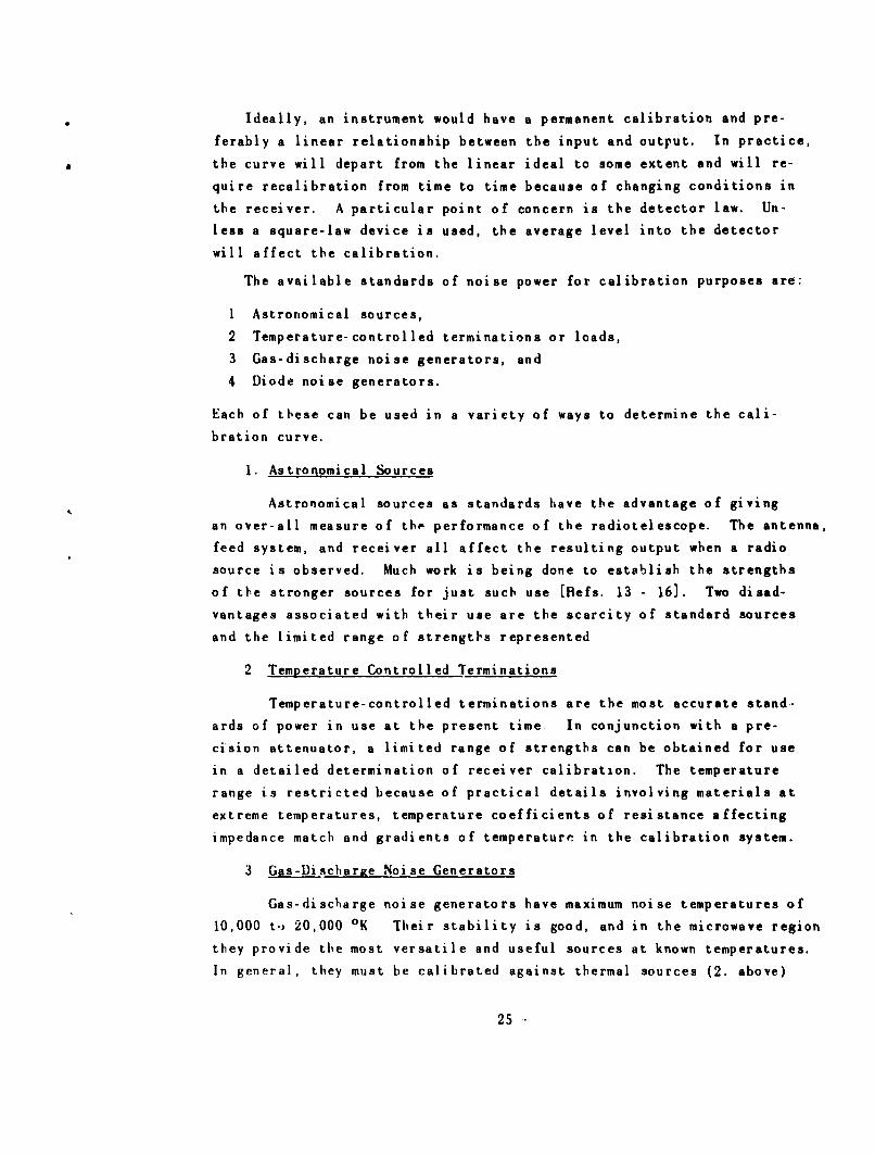
The available standards of noise power for calibration purposes are:

1 Astronomical sources,

2 Temperature-controlled terminations or loads,

3 Gas-discharge noise generators, and

4. Diode noise generators.

Each of these can be used in a variety of ways to determine the cali-

bration curve.

1. Astronomical Sources

Astronomical sources as standards have the advantage of giving

an over-all measure of tho performance of the radiotelescope. The antenna,

feed system, and receiver all affect the resulting output when a radio

source is observed. Much work is being done to establish the strengths

of the stronger sources for just such use (efs. 13 - 16]. Two disad-

vantages associated with their use are the scarcity of standard sources

and the limited range of strengths represented

2. Temperature Controlled Terminations

Temperature-controlled terminations are the most accurate stand-

ards of power in use at the present time. In conjunction with a pre-

cision attenuator, a limited range of strengths can be obtained for use

in a detailed determination of receiver calibration. The temperature

range is restricted because of practical details involving materials at

extreme temperatures, temperature coefficients of resistance affecting

impedance match and gradients of temperature in the calibration system.

3 Gas-Discharge Noise Generators

Gas-discharge noise generators have maximum noise temperatures of

10,000 to 20,000 OK Their stability is good, and in the microwave region

they provide the most versatile and useful sources at known temperatures.

In general, they must be calibrated against thermal sources (2. above)

25-

4. Diode Noise Generators

Diode noise generators have a somewhat lower frequency range, ex-

tending down from the lower microwaves. To obtain good accuracy with a

diode noise source care must be used in the measurement of diode current

and in the provision of a good termination over the frequencies of inter-

est These noise sources also must be calibrated against thermal-noise

sources

5. Recalibration

The receiver must be calibrated frequently enough to provide the

desired accuracy. Sometimes a calibration procedure must be carried out

before and after each measurement of a series, while sometimes a partial

calibration only at one or two points need be inserted several times in

the course of observation. Naturally the quality of the instrument de-

termines how often calibration is necessary.

A typical calibration curve for a total power receiver is shown

in Fig 3.1 Deflection of the output meter is plotted against signal

input with the point for zero signal indicated. The curve is shown ex-

trapolated to a zero for total noise input, which is Tes degrees below

the signal zero.

C. EXTREME GAIN-STABILITY REQUIREMENTS

Total-power receivers have been constructed and used with effective

input temperstures from a few hundred to several thousands of degrees

Kelvin Typical UL's, as calculated from theoretical receiver parameters,

go as low as a few parts in ten thousand. It is evident that, in order

that the receiver be fully utilized, it must be stable tu 4 similar ex-

tent. In order to achieve stabilities on this order, one must to begin

with, use power sources that are sufficiently stable and then design the

receiver itself to be as free as possible from other sources of instabil-

ity Finally, operation in a controlled environment is very important.

As well as providing a receiver as stable as possible, one resorts

to calibration checks as frequently as practical in an effort to mini-

mize the effects of the remaining instabilities Many receiving systems

perform part of this calibration function as part of their mode of opera-

tion, with the type and amount of stabilization achieved depending on

their system design For instance, the Dicke receiver can be thought of

26 -

DEFLECTION

ZERO-SIGNAL PO!NT ----

0 O SIGNAL INPUT (1K)

FIG. 3.1 TYPICAL CALIBRATION CURVE FOR A TOTAL-POWER RECEIVER SHOWINGTHE ZERO-SIGNAL POINT AT AN APPRECIABLE DEFLECTION. THE DOTTED EXTRA-POLATION YIELDS A ZERO FOR TOTAL NOISE INPUT T., DEGREES BELOW ZEROSIGNAL.

as one which, at the modulation frequency, provides automatic partial

calibrations spaced from each uther by very short intervals of time.

D. TYPES OF STABILIZATION

For a receiver that is ideally linear except for the detector-powerresponse, we can express the calibration curve (z vs. T) for changes in

signal temperature T as

z(T) - f(K, K 2, Tes, T)

for a given detector law. Here K, is the power gain before the detector,

K2 is the voltage gain after the detector, and T., is the average effectivesystem nois4e The detector output is a function of the total power at

its input, represented by TT. This output can be expanded in a Taylor

- 27

expansion about the TTUTea level, where signals are then represented by

T - TT -Tea, thus

y(T) - g(KITe.) + g'(KIT,.)KIT + g"IT..) (KIT)2 +

With the gain factor K2 applied,

g'"(KITe)

z(T) - K2y(T) - g(KIT..)K 2 + g'(KIT*5 )K2KT + 2! K2(kT)2 + (7)2! (T)+ ()

When considering minimum detectable signals with T zero,

z(O) - K2 g(KiTe.),

which has three variables--K 2, K1 , and Tea'

1. Zero-Point Stabilization

Zero-point stabilization is achieved when z(O) is independent of

gain and system noise A servo system that compares z(O) against a

standard and operates on the receiver gain to make z(O) equal to the

standard can produce zero-point stabilization. Gain changes will be

corrected if the servo operates to change KI. Changes in Tea, however,

will require a compensating change in gain that changes the scale of the

calibration curve. The detector operating level will be held constant

so that the shape of the calibration curve will change only as a large-

signal effect (The coefficients gi(KIT e.) in Eq. (7) rema.n constant

but the (KIT)' factors become significantly changed for large signals.)

Figure 3.2 shows a gated AGC system with these characteristics.

Another way of assuring z(O) equals a constant is by making

g(K1ie5 ) equal to zero The Dicke receiver does not respond to Tea and

hence effectively sets z(O) - 0 In this, then, receiver-gain changes

result in changes of calibration-scale factors and Tea changes have no

effect directly. Since the detector level is not maintained in any way,

both gain and Tea changes will tend to shift the operating level and thus

can change the calibration Figure 3.3 shows such a Dicke receiver and

the resultant calibration curves for changes in gain and Teo,

- 28

I' ANT

AC

DETECTOR OPERATING POINT ODNSTANT BUT CALIBRATION CHANGES

DEFLECT ION b

CONSTANTZERO-SIGN4AL

POINT

]~TL *~~0 SIGNAL INPUT (*K)

FIG. 3.2 GATED AGC. GATED TOTAL-POWER RECEIVER WITH ZERO~-SIGN4AL POINTSTABI LI ZATION

-29w

REF. RCIE

NEI7HER DETECTOR OPERATING RFONT, NOR CALIBRATION CCNSTANT

DEFLECTION

POINT

0 ~SIGNAL INPUT (OK)

TO$ x GAIN____-

FIG. 3.3 DICE-TYPE RECEIVER WIIh ZERO-SIGNAL POINT STABILIZATION.

- 30 -

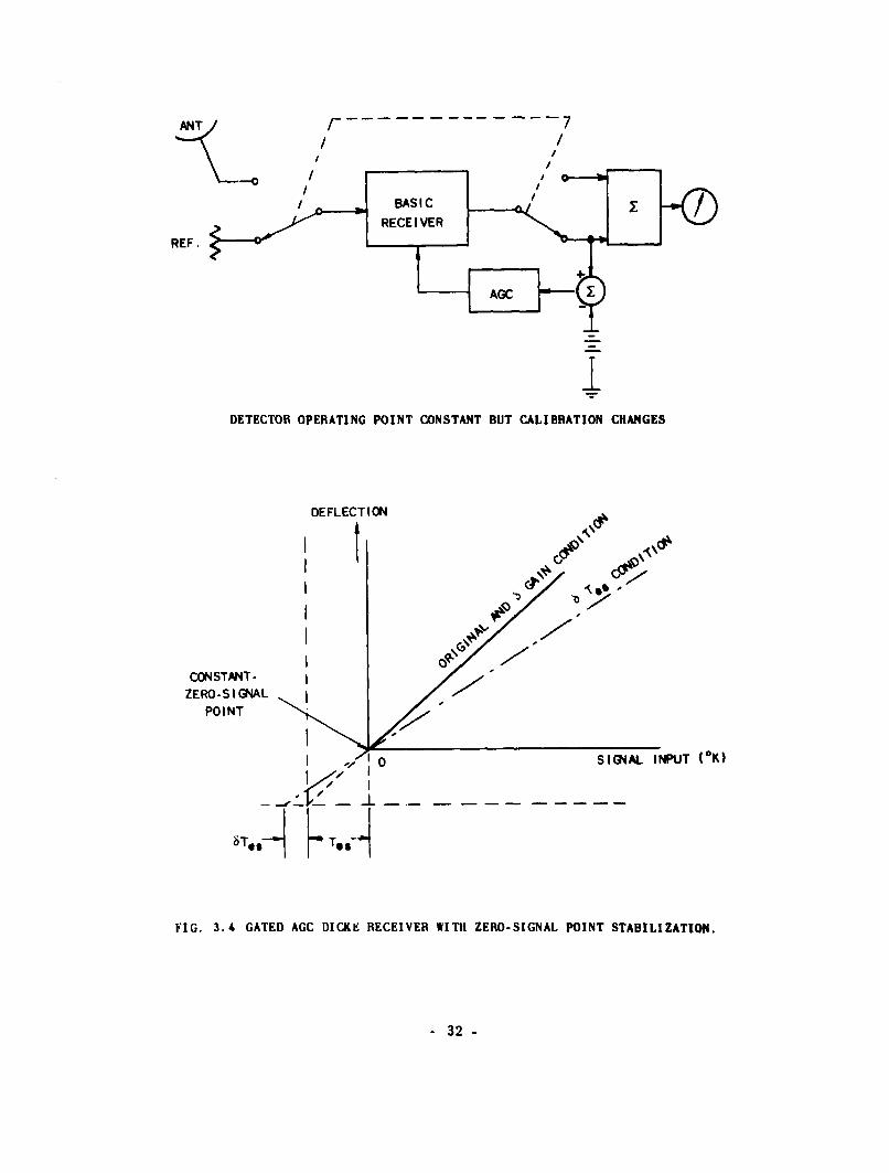
Another possible zero-point stabilization method is to use a com-

bination of the two systems above [Ref. 71 Figure 3.4 shows such a re-

ceiver with a Dicke signal output but gated AGC. This receiver maintains

constant calibration-scale factors with gain changes but not T., changes,

in contrast to the straight Dicke receiver, in which the opposite is true.

2. Two-Point Stabilization

Two-point stabilization is achieved when two fixed inputs result

in two fixed outputs. The control of the two gain variables K, and K2

is not sufficient to ensure that the calibration curve will pass through

two points, in general, unless we make z(O) = 0 in some way. Then control of

only one gain variable can force the calibration curve through a desired

point as well as the constant-zero signal point. If we can control both

gain variables, then the detector operating level can also be held con-

stant. Figures 3.5 and 3.6 show block diagrams and calibration-curve

sketches for two point-stabilized receivers. Information concerning the

three input levels must be recoverable at the receiver output through

suitable modulation techniques. The receiver shown in Fig. 3.6 has the

two servo gain controls and maintains the detector operating level con-

stant.

When the characteristics of the receivers are not known explicitly

it is difficult to predict whether two-point stabilization with or with-

out maintaining detector operating level will be more advantageous. The

one showing the least departure from the original calibration curve over

the range of signals expected would be most desirable These facts point

out the great advantage of a linear power response (such as the ideal

square-law detector provides) which eliminates detector-operating-level

problems.

The slope of the calibration curve can be stabilized by using the

additive modulation scheme shown in Fig. 3.7. A modulated component is

added to the total noise input and the receiver gain is adjusted to keep

the output constant for this modulated component. This process permits

the effective sensing of the slope of the calibration curve and keeps

the slope constant for large dynamic ranges. As shown, however, the zero

signal point is a function of Tes This arrangement can be called a

modulated pilot-signal, total-power receiver.

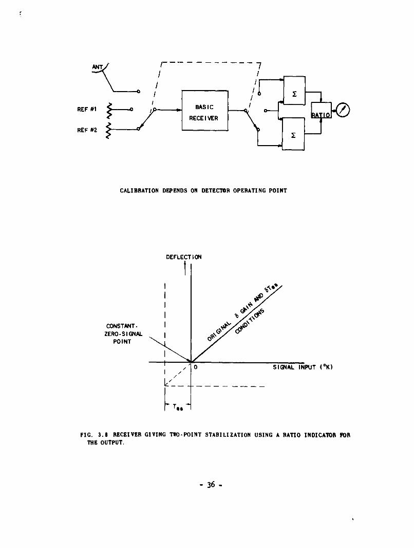
Another system that achieves two-point stabilization uses a ratio

indicator for the output Figure 3.8 shows the block diagram of such a

receiver with two reference sources time shared with the signal and two

- 31

REF.I t

DETECTOR OPERATING POINT CONSTANT BUT CALIBRATION CHANGES

DEFLECTION

710

CONSTANT-

ZERO-SIGNAL -

POINT

I .. 0I SIGNAL INPUtT (OK)

FIG. 3.4 GATED AGC DICKE RECEIVER WITH ZERO-SIGNAL POINT STABILIZATION.

- 32

ANTI-II

REF #1BAIRECE IVER

REF #2

CALIBRATION DEPENDS ON DETECTOR OPERATING POINT

DEFLECTION

I

CONSTANTZERO- SI!GNAL "

POINT

0 S SIGNAL INPUT (°K)

FIG. 3. S DUAL-REFERENCE MODULATED RECEIVER WI 7H ONE SERVO GAIN CONTROL PRO-DUCING TWO-POINT STABILIZATION.

- 33 -

ANT

REF #1 AMP. DETECTOR AMP .

REF#2

CALIBRATION UNCHANGED WIlI 'e OR b GAIN CHANGES.

DEFLECTION

ZERO.SIGNAL

1 /"0 SIGNAL INPUT (0 1K)

I,

FIG. 3.6 DUAL-REFERENCE MUJULATED RECEIVER WIIH TM SERVO GAIN CONfTROLS PRODUCINGTWO-POINT STABILIZATION AND CONSTANT DETECTO R OPERATING POINT.

- 31f -

PNT

BAISILICU (K

FIG. .7 DULAED PLOTINLTOA-OERRCEVR

MOD . 35

ANT I 7

REF #1RECE IVER

REF #2

CALIBRATION DEPENDS ON DETECTOR OPERATING POINT

DEFLECT ION

I

CONSTANT- IZERO-SIGNAL I

POINT

L1 40 SIGNAL INPUT (0K)

FIG. 3.8 RECEIVER GIVING TWO-POINT STABILIZATION USING A RATIO INDICATOR FORTHE OUTPUT.

- 36 -

coherent demodulators providing measures of the strength of the signal

relative to one reference and the difference in strengths between the two

references. 7he ratio of these two measures is zero for equal signal and

compared reference strengths, regardless of gain or T., conditions. The

calibration depends on the detector operating level but is otherwisestabilized.

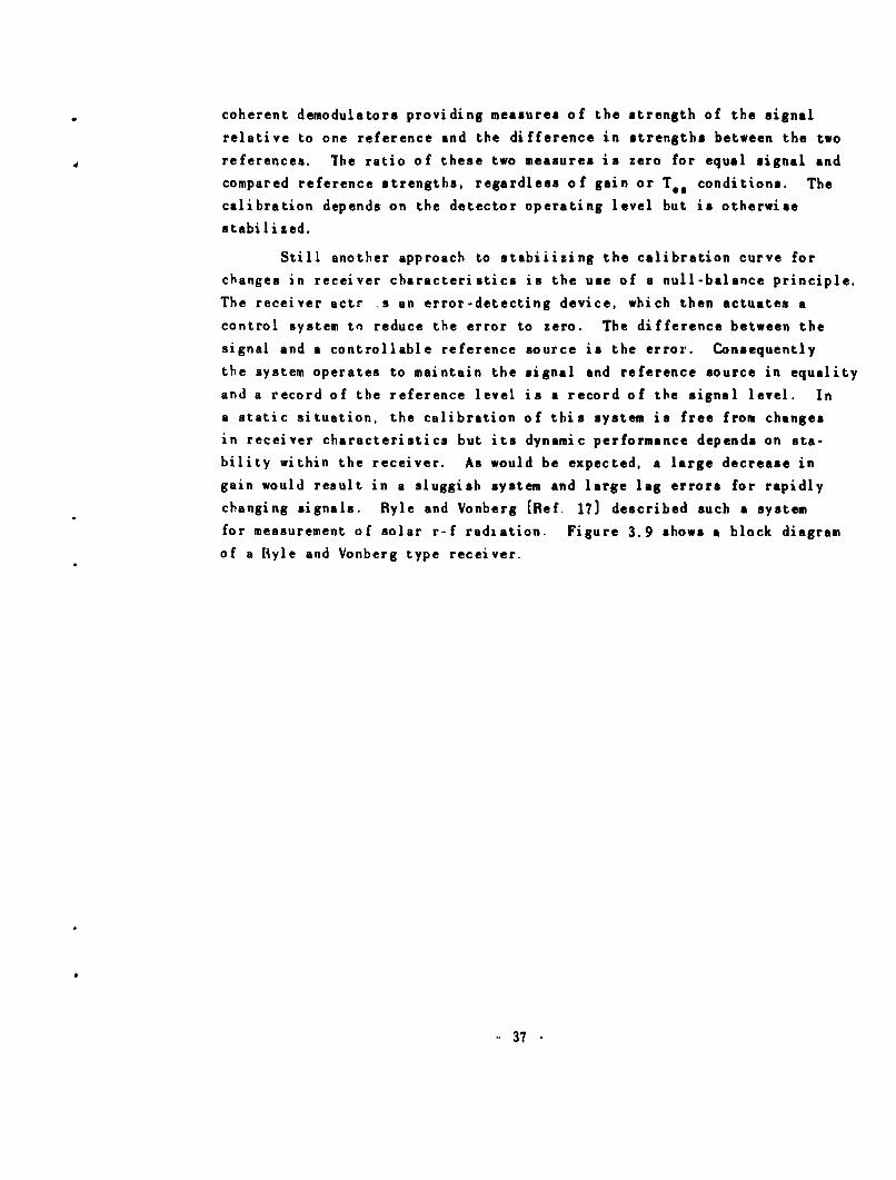
Still another approach to stabiiizing the calibration curve for

changes in receiver characteristics is the use of a null-balance principle.

The receiver actr .s an error-detecting device, which then actuates a

control system to reduce the error to zero. The difference between the

signal and a controllable reference source is the error. Consequently

the system operates to maintain the signal and reference source in equality

and a record of the reference level is a record of the signal level. Ina static situation, the calibration of this system is free from changesin receiver characteristics but its dynamic performance depends on sta-

bility within the receiver. As would be expected, a large decrease in

gain would result in a sluggish system and large lag errors for rapidlychanging signals. Ryle and Vonberg [Ref. 17) described such a system

for measurement of solar r-f radiation. Figure 3.9 shows a block diagram

of a Ryle and Vonberg type receiver.

-37

BA II

ZEROSERVO

POINT ________________

0 SIGNAL INPUT (OK)

FIG. 3.9 NULL-BALANCING RECEIVER STABILIZED AGAINST GAIN AND T., CHAN4GES AND

INDEPENDENT OF DETECTOR OPERATING POINT.

- 38 -

IV. MORE-ODMPLEX RECEIVERS

A. STABILIUED RECEIVERS WITH UNMOIJLATED SIGNAL

As mentioned earlier, two of the approaches to achieve freedom from

instabilities applied to radio-astronomy receivers are d-c comparison

techniques such as reported by Selove and correlation techniques such as

discussed by Goldstein. Both of these methods use two channels and de-

pend on the statistical independence of the two sources of equivalent

input noise.

I. Selove-Tyie Receivers

Zero-point stabilization is the goal of receivers of the Selove

type. The zero signal output of the total-power receiver depends on the

gain and T., of the equipment, and subtraction of a fixed d-c level from

the output does not alter this dependency. However, if it were possible

to subtract a level which was a function of gain and Tea, the resulting

output could be zero-point stabilized Consider a receiver which has

twin channels for amplification, detection, and smoothing. To the first

order of approximation, gain and T., changes are the same in both channels,

so that, if a fixed noise-temperature input is provided for both channels,

the outputs (including instability contributions) will have the same mean

values and a resulting zero mean difference. To the extent that this

approximation is true in a practical system, the Selove-type receiver is

zero point stabilized Figure 4.1 shows a block diagram for receivers of

this kind.

The output of each channel will have an equal rms variation about

its mean and the difference between these two will have an rms variation

that is v/2 times an individual value If one of the two identical chan-

nels has

UL - 1 f

then the Selove-type receiver has

UL - Y"2 / /fAi (8)

In order to compare this with other receivers, the extra channel

bandwidth should be accounted for by allotting the total signal and

39 -

S I GNAL

SIGNAL CHANNEL DETECTOR FILTER

F IXED- CPRSON CHANNEL DETECTOR -o 1. G

NOISE FILTER

I NPUT ________

FIG. 4.1 BLOCK DIAGRAM OF A SELOVE TYPE "D-C COMPARISON" RECEIVER.

comparison bandwidth to the other receiver. When this is done the Selove

receiver has a value of AT twice that of a total power receiver. The

ratio

AT 1 . v2 / v1rLf 2Total Power I vr A

Operation with a comparison channel using parameters differernt

from those of the signal channel is possible. In general, the signal,

by its nature, will determine the integration time required. If the

comparison channel had less integration time, the output would be noisier

than necessary, and if it had more the instability spectrum above the

cutoff frequency of the comparison channel smoothing filter and below

the cutoff of the signal channel smoothing filter would tend to produce

pseudo-signal outputs. Therefore, equal integration times is a reason-

able situation

For differefnces in reception-filter bandwidths, consider the follow-

ing. For an ideal d-c comparison receiver we have plotted AT/ATstd, (the

dashed curve in Fig. 4.2) the ratio of its AT to that for a standard total-

power receiver with the same signal bandwidth ATstd, against the ratio of

comparison-channel bandwidth Afc to signal-channel bandwidth AfU. As the

comparison-channel bandwidth becumes larger, the performance approaches

that of the standard receiver and at low-comparison bandwidths it is much

worse. When UfC/ Sf • 1 the value of the ratio is v , as would be ex-

pected from Eq (8). A further comparison is provided by the solid

- 40 ..

In o inN ' -J -* I. . /~ Ig U -br,?,, j ?/

U 1.1

I.

-- /1/

curves in Fig. 4.2, which show the ratio /T/ATstd for a family of total-

power receivers with different instability factors y. The bandwidth for

these receivers is taken to be equal to Af.(l + (Afc/Af.)] or all the

bandwidth is used in the signal channel. When y - 2 the d-c comparison

receiver yields larger AT's for all bandwidth ratios except unity, in

which case the two are equal.

For a stable receiver with y small, the total-power configuration

has an advantage, but as y increases the d-c comparison receiver has asmaller AT. In practice, the comparison receiver will be non-ideal, so

that its curve would be raised and its relative advantage would be re-

duced. Thus we can say that, for conditions under which the total usable

bandwidth is not limited for other reasons and a reasonably stable re-

ceiver can be achieved, the extrr bandwidth of a second channel is more

useful for signal than for d-c comparison purposes.

To approximate the condition of identical instability behavior,

the two channels would have to be obtained by band filtering at the input

and output of a sufficiently wideband amplifier. This requirement places

a strict condition on relative bandwidth stability for the channels and

is probably the most difficult requirement to meet in obtaining good

performance from a receiver of this type.

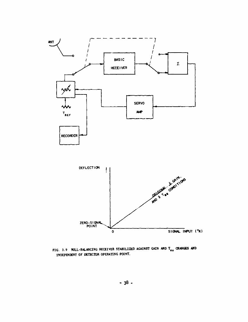
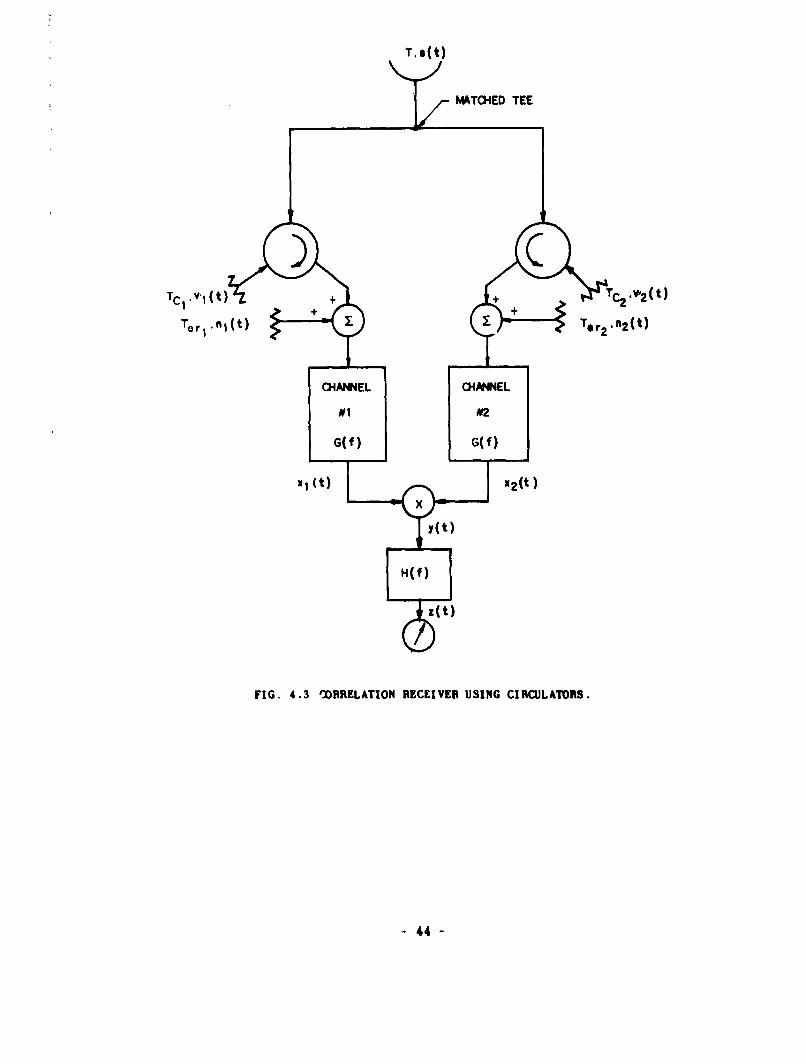
2. Correlation-Type Receivers.

This classification could well be called autocorrelation receivers

when used to describe operation using a single signal input, in contrast

to interferometer radiotelescopes using two inputs. Signal processing

begins with a splitting of the input into two equal and necessarily

fully correlated signals. These are separately equally amplified and in-

variably degraded with independent receiver noise and then multiplied

together. The product signal is then smoothed with some integrating time

and the result appears at the receiver output as a meter deflection. The

ideal process can be described in mathematical terms as follows, letting

s/vi be one half the signal on a power basis:

z(t) - [(a/v'2) (t) • (a/v/ ) (t) * h(t).

The smoothing filter impulse response is h(t), which can be written out as

t

z(t) I f s2(t) h(t- t') dt'. (9)2 _M

-42 -

This equation can be compared with

t

Pa(tT')l i f atW) 1 dt', (10)

the value of the autocorrelation function for a(t) at any epoch t and with

zero time displacement between a(t) and itseif. When T grows large the

function p.(0) changes very slowly, so that Eq. (9) will be nearly equal

to Eq. (10) when the equivalent width of the smoothing filter impulse re-

sponse corresponds to large 7 values. To the degree that this approxima-

tion holds, an autocorrelation is being performed; hence the name.

A prime problem in receivers of this type is the necessity of

splitting the signal and at the same time preventing the coupling of noise

from the input of one receiver channel to the other. This coupled ',oise

would appear at the multiplier as a correlated component and hence pro-

auce a zero-signal deflection. Since the idea is to have no zero-signal

deflection in order to stabilize the system against gain changes, such

coupled noise is undesirable.

A matched-tee junction in a waveguide, or its equivalent in other

transmission lines, is a convenient method of splitting the signal equally.

Coupling is still present, however, therefore, further steps must be taken

to control this factor. When isolators are inserted between the tee and

each receiver an improvement is possible since the source of the coupled

noise then is divorced from the input of each channel and becomes well

behaved. The equivalent coupled-noise-source temperatures are then equal

to the isolator temperatures A step beyond this configuration is to use

circulators in place of isolators as shown in Fig. 4.3. Then the noise

sources are not only known but are terminations that can be refrigerated

if desi,.ed In any event, the analysis of the circulator case covers

the othe.- two and makes the noise sources easily visualized.

In Fig. 4.3 the noise voltages s(t), v1 (t), v2 (t), n1 (t) and n2(t)

are all related to an equivalent noise source by a relation such as

<s 2 > - 4kTR f G(f) df

- O

ur

<v 2 > - 4kTc R f G(f) df

43

T, 8(t)

MAT04ED TEE

TC1, Vij(t) + + + T 2. '2 (t)

Tr n, (t) T TrR2 (t)

CHANN4EL CHANNEL

FIG. 4. 02LTONRCIE SNGC~U OS

G~~f4 -~f

The matched-tee junction splits the energy coming from the antenna so

that a power <s2>/2 appears in each branch along with the voltage s//2.Energy flowing from the circulator load towards the matched tee meets a

mismatch at the junction and an unequal division of energy occurs. The

power in the antenna line is one half, the power in the line to the other

receiver is one quarter, and the power reflected is also one quarter of

the input power. Energy flowing toward the antenna will be radiated while

the components flowing from the junction to the receivers will constitute

a completely correlated but opposite-polarity signal. Thus each circu-

lator load produces at the output a negative meter deflection. Noise

sources at the receiver inputs produce energy flowing toward the circula-

tors, where it is absorbed in the circulator load.

For this receiver the mean meter deflection will be

< <52/2> - <v2/16> -<v2/16>

In practice the zero-signal condition will not mean T - 0 because of the

equivalent noise temperature of the system before the tee junction. The

mean meter deflection with zero signal can be nulled if the temperatures

TcI and T"2 are properly maintained.

Appendix B contains the analysis for the correlation receiver of

Fig. 4.3. With the approximation that the smoothing filter is much

narrower than the reception filters or the integration time muct. longer

than the correlation time of the random voltages at the multiplier input,

the analysis is straightforward. In evaluating the autocorrelation

function pY(T) for the multiplier output we have used the general relation-

ship below for gaussian random-noise voltages with zero mean values from

well behaved processes, which gives the time average for a product of

four such variables in terms of products of pairs of the variables [Ref. 18].

For the term involving the receiver noise, for instance,

<nl (t )n 2 ( t)n l (t + )n 2 (t+ 7> -<nl(t)n2(t)> <nl(t+-)n2(t+)>

+ '<nl(t)n(t+7)> <n2(t)n2(t+"r)'>

+ <nl(t)n2(t+)>'<n2(t)nl(t+r)>

a Pn1(r) P.2( r).

.. 45 -

After reducing the expression for p (r) to the sum of terms obtained as

above, its Fourier transform is taken to obtain B (f), the power spectral

density at the multiplier output. The smoothing-filter power-transfer

characteristic is then applied to obtain the receiver-output power

spectrum. From this we can write

'<z> - k[H(O)] fo G(f) df[(T/2)-(TC /16)-Tc/16)]

for the meter deflection and

S - k[H(O)] G(f) df (AT/2)-C

for the signal or mean meter deflection increment due to an input tempera-

ture increment AT. The noise output will be

N a H f) df k[G*GI 0 T oo,

Now, using unity signal to noise ratio to define 6T, we write

k[H(O)] % G(f) df (tT/2)

SIN - I - -

k f H(f) df [G*GI °0' Tea

and

LT 1(1VVrtf) Teo

following the definitions for bandwidth and integration time discussed

above.

The system effective noise temperature Tea contains contributions

from all the noise sources as given below:

- 46 -

Tm T 8'Te2 + (T/2) (Ter +T G2) + ((Ter TC +TerT 2 )/16)1

+ [(Ter TC +Tr T C )16 +(T2/2) + (T1T 2 /4

+ [(TC,2+TC2 )/128 %

For the case when

Ter *Te *Tor

and

TC I TC2 0

we have

Te CT ar 2+ TTor + (TorTC/4) + (T2/2) + (TC/32)) %

a Terfi + (T/Ter)4TC/4Tr(T2/2Tr*+(1C /32Ter)]

When

I/Te <or

and

TC/Ter '< 1

we can write

Tea Tor (1 +(1/2Tor )(T + (TC/4fl}

STer + ('1/2) + (C8

-47 -

Gain changes produce changes in the output when [I -(Tc/4)] does

not equal zero. Following Bracewell (Ref. 8, we form the ratio of mean

meter deflection for the correlation receiver to that for a total-power

receiver to obtain an instability-reduction factor

[T- (Tc/4)]/2T + Tr

to be applied to the contribution I (see Eq. (6).

The correlation receiver of Fig. 4.3 has been shown to have a

1.414-times larger minimum detectable signal than a total-power receiver,

but again using twice the total reception-filter bandwidth because of

two channels. On this basis the comparison factor should be two. Zero-

signal-point stabilization is possible by temperature control of the

circulator loads and partial stabilization is assured since receiver

noise contributions are eliminated.

When a matched tee without circulators is used, the receiver noise

sources feeding the antenna take the place of TCl and Tc2 in the analysis

of cross-coupled noise. Since little, if any, control is possible on

these noise sources, the receiver has mainly the advantage of removing

mean meter deflections due to receiver equivalent input noise Tar plus a

minimum detectable signal only 1.414 times that of a total-power receiver.

With isolators a similar statement holds, but with the advantage,

as mentioned above, of well defined sources at known temperatures for

the cross-coupled noise.

When a matched hybrid junction or magic tee is used to split the

signals, the multiplier input consists of voltages similar to those of

the previous discussion In Fig. 4.4, the fourth port of the magic tee

has a termination at a temperature Tj that provides noise energy for the

two channels of opposite polarity but correlated voltage. This energy

splits equally, so that the voltage in the channels will be t 1/v'2. The

corresponding value for Tea for this receiver will then be

Tea [Ter 2 +TTer +TjTer + T2 +Tj %

Ter + (T/2) + (Tj/2)

48

T.S(t)

MATCHED Tj. f(t)MAGIC TEE

+ Tr2+ +

ft (t) n2 (t)

FIGHA.NNELAONECVEUSGA MICHTATEL

NP

- 9

while the mean meter deflection will be proportional to

(T/2) - (Tj/ 2 )

Although Tj would have to be maintained at a lower temperature than Tc

in order to null the zero-signal mean meter deflection, the magic tee

has the advantage of avoiding any signal-path loss of circulators.

Thus far in discussing correlation receivers, the multiplier has

been assumed to be an ideal element. Practically they represent a dif-

ficult portion of the receiver to implement. Blum (Ref. 9] discusses a

type of multiplier that uses essentially the quarter-square-difference

principle. He suggests connecting the two-channel outputs to two ports

of a hybrid junction, with the result that sum and difference signals

appear at the other two ports. Each of these is squared in a square-law

detector and finally the detector outputs are subtracted to get the

product term. When this method of multiplication is used with the re-

ceiver of Fig. 4.4 the mean meter deflection will be

'<z> a <52> .<12>

k(H(O)]% f G(f) df (T-Tj)-0

The relative noise output for this multiplier is the same as that

of an ideal device and, consequently, the minimum detectable signal is

the same, i.e.,

AT V T I

where

Tea - Ter {I + (T +Tj)/2TerI}.

From these considerations we see that the correlation receiver can be

realized in this manner without sacrificing performance if care is taken

with the practical difficulties such as balancing of the hybrids and

duplication of detector responses

- 50 -

B. STABILIZED RECEIVERS WITH MODULATED SIGNALS

1. Introduction

Several receivers fall into a mixed classification. For instance,

a correlation receiver can be designed to use time sharing of a single

channel, using the quarter-square multiplication process. With this

process, alternately, the sum and the difference of a split input signal

are squared, with alternate-period outputs subtracted from each other and

a final smoothing performed. This process could also be described as asignal modulation, since in the sum periods the signal power is present

while in the difference periods the signal power is cancelled out. Further-

more, this process has the characteristics of a phase-switched system in

that sum and difference signals can be formed by switching a 180-deg

phase shift in and out of one split-signal channel.

Receivers that fit these descriptions will be handled as modulated-signal receivers. The method of stabilizing a receiver as described by

Dicke (Ref. I] is the classic example of a receiver that uses a modulated

signal. This type of receiver keeps the signal information identifiable

in the total noise with a signal modulator ahead of as much of the noisy

portion of the system as possible. At the output, knowledge of the

characteristics of this modulation allows the extraction of the signal

and at the same time, the supression of the d-c component due to Tes.

2. Dicke-Type Receivers

In Dicke receivers the effective input-temperature modulation is

proportional to the signal strength and demodulation is performed ro-

herently after detection to obtain a measure of the signal. This measure

is presented on a meter, which, in the absence of signal and hence of

modulation, has a zero mean deflection.

The receiver input is commutated between the signal source and the

reference source by the modulator. This commutation occurs periodically

at a frequency f. and the effective modulated input temperature can be

written

T -q (t) T + (l - 7(t)] Tref

where Tref is the noise temperature of the reference source and I is that

.f the signal source. This form of expression comes from considering a

variable attenuator in the signal path whose power-transfer characteristic

- 51 -

as a function of time is 7(t) and whose attenuating element is at tem-

perature TrefL For sinusoidal modulation the function

77(t) - U1 +con 2,nfmt)/2

or, for square-wave modulation,

77(t) {1 + (4/7)(cos 277f t- (1/3) cos 23ft + (1/5) cos 275f t- ... )}2

or, in general,

( t) *.+1n. KM exp ( 2T2 2 nu n (jn2vfst)

[1 +/(t)]/2

The function /M(t) determines the modulation waveform For sinusoidal

modulation /i(t) is sinusoidal, for square-wave modulation p(t) is square-

wave, etc. The restriction that T, be positive requires that

ki(t)l I 1max

A rather qualitative discussion that gives the minimum detectable

input-temperature increment for square-wave modulation follows.

An ideal switch alternately connecting the signal source and the

reference source to the receiver input will produce square-wave modula-

tion The effective receiver-input-noise temperature source is con-

nected at all times. On the average, the detector output during the twohalves of the cycle will be proportional to the sum of T Pnd Ter and the

sum of Tref and Ter The standard deviation from the mean for an indi-

vidual half-period (1/2fM) average of the detector output can be written

a s cc (T + T e r ) ~ -m

for the signal and

- 52 -

aref cc (Tref +Ter) 2/M

W for the reference. The receiver output will be proportional to the dif-

ference between the mean value in the two conditions, and this measurement

will have a standard deviation that is the quadratic sum of aS and aref"

For the case in which t and Tre f are equal, the standard deviation for

the output expressed as the minimum detectable input-temperature incre-

ment will be

AT - V (T +Te) /2 f/Af

S2(T + Tor ) *, f/6f (25)

We see that the M factor for this mode of operation equals 2, twice that

for total-power operation using a smoothing filter with r a l/f=. One

vr factor (from the value of M) comes from the need to compare two equally

noisy levels and the second because the time spent observing either level

is half that possible with total-power operation. (This reduction in

observing time enters into the expression for AT above as a value of r

one-half that possible with total-power operation.) Further smoothing

affects both systems equally and hence does not change the modifying

factor M - 2.

For a switch that spends unequal times in the two positions, fbeing the fraction of the switching period spent in one position,

AT - (T+Tref) Vf/Af V/i/1A( ./A)

Since this expression is a minimum for /8 1 1/2, square-wave switching can

be considered optimum and the value of M * 2 a minimum.

Appendix C contains a detailed analysis of a modulated receiver.

The block diagram in Fig. 4.5 shows the generalized form for this re-

ceiver. The modulation considered here is a power modulation; i.e.,

the modulator output power is made to vary in a specified manner. Dicke's

(Ref. I] receiver used a rotating attenuator in the input waveguide and

obviously falls in this category. Goldstein (Ref. 19] and Strom (Ref. 20)

discuss sinusoidal-voltage modulation, which seems to be an artificial

- 53 -

LAL

LLI-. I

> LL.41I3%,

-54-

situation, although it can be shown to yield the same results as

sinusoidal power modulation in the cases they considered.

After the detector, two components are added that are not present

in the total-power receiver.-the video filter and the coherent demodulator.

The second of these is essential while the use of the first is controlled

mainly by practical considerations. Frequently, in order to avert over-

loading in stages just prior to and in the coherent demodulator, it be-

comes advisable to limit the noise power by a rather narrow filter. This

filter, whose power-transfer characteristic is K(f), is made wide enough

to avoid trouble with phase shifts and amplitude changes produced by

drifts of tuned circuits and modulation generators. Therefore, the smooth-

ing filter determines the noise bandwidth after detection.

The coherent demodulator can be described as a multiplying element

in which the product of a signal and a reference voltage is produced. The

signal output is at a d-c voltage level depending on the amplitude of the

signal input and its phase relative to that of the reference voltage. A

simple form for a coherent demodulator and smoothing filter is shown inFig. 4.6.

The first step in the analysis consists of setting up a form for

the voltage x(t) that gives the proper power levels out of the detector.

Then, using this expression, the signal and noise powers through the rest

of the receiver are calculated from autocorrelation functions and their

transforms. It is necessary to take averages over statistically long

periods in order to apply autocorrelation- function techniques. Since

these long ieriods must be short compared with modulation periods, we are

left with the requirement that has been assumed for this analysis, that

fm is much smaller than f.

The resulting expression for 8T is a function of /(t) and (t).

After combining these into a factor M, we have the expected form

6T - M(T +Tre f) rIU

The values of M for different modulation [M(t)) and demodulation tg(t))waveforms have been calculated. When, for the video filter, J(f) * 1,

M - 2 i< (t)2>/[(l/7) j /(t)e(t) dt] 2

0and values are given in Table 4.1.

- 55 -

- CONTOLLED BY (t)

I/

YFltM

FIG. 4.6 COHERENT DEMODULATOR WHICH IS AN IDEAL SWITCI DRI-

VEN BY THE REFERENCE VOLTAGE e (t). TIE SWITCH ACTION MUL-TIPLIES YF(t) BY A SQUARE WAVE.

TABLE 4.1. VALUES OF THE MODIFYING FACTOR M IN THE FORMULAFOR AIT FOR THE CASE OF NO VIDEO FILTER [J(f) u I].

Demodulation Values of N for Modulating Waveform )&(t)

Waveform f(t) Square-wave Sinusoidal Sawtooth

Square-wave 2.00 v a 3.14 4.00

Sinusoidal ,IV'- 2.22 2Vi - 2.83 W72 - 4.44

Swtooth 4 /43 • 2.31 2,,/V - 3.63 W3 - 3.46

When the video filter passes only the fundamental component of the

modulation,

M - 2/IK4 I

where 1K j is the magnitude of the coefficient for n - 1 in the following

expression for p(t):

- 56 -

p( t) Kn exp(jn277f t)

Values for M in this case are given in Table 4.1.

TABLE 4.2. VALUES OF THE MODIFYING FACTOR MIN THE EQUATION FOR AT FOR A NARROW-BANDVIDEO FILTER THAT PASSES ONLY THE FUNDAMENTALCOMPONENT OF THE MODULATION WAVEFORM u(t).

ModulationWaveform A(t) M

Square-wave W2 - 2.22

Sinuaoidal 22 - 2.83

Sawtooth W2 - 4.44

The qualitative discussion that led to a squale-wave operation

for a least AT is upheld with the value M - 2 applying in the case of A.(t)

and f(t), both being square-waves, and J(f) - 1. In this case also we

can state that, for a given modulation waveform, the least M occurs when

e(t) is of the same form. With the narrow video filter, M is seen to be

independent of (t) except for its relative phase. Only the amplitude

of the fundamentel frequency component of ji(t) enters the expression.

In the presence of instabilities, the modulated receiver provides stabili-

zation of the zero point on the calibration curve. When operating optimal-

ly in this sense, the condition of zero-signal input results in a zero-

mean meter deflection. The manner in which instabilities affect the

modulated receiver's performance is discussed below

Instabilities in receiver components ahead of the detector modulate

the power into the detector and contribute to the power spectral density

of the detector output B J(f). These contributions can be avoided by

proper choice of fm as discussed above. Instabilities after detection

and before demodulation increase the noise-power spectrum uniformly across

the band passed by the video filter and hence contribute to output-noise

- 57 -

power even under zero-modulation-component conditions. Considering these

instabilities also as a modulation effect, the spectrum of the noise into

the demodulator will be that of the video-filter output convolved with

the spectrum of instabilities producing the modulation and an impulse

function -if unit area representing stable transfer conditions The noise

spectrum will be widened and increased in amplitude in this process.

Figure 4.7 shows typical spectra involved in this effect.

Therefore, even with a zero-mean meter deflection, an increase in

the fluctuating neter-deflection component occurs, depending on the

stability of the receiver components between the detector and the de-

modulator. Fortunately, the gain required in this section of the re-

ceiver can be achieved with amplifiers using heavy negative feedback

and having consequently a higi degree of stability. In the following

paragraphs we assume that the effect is negligible.

At times, operation with a fixed difference in temperature between

the antenna and the reference is necessary. For instance, the reference

may be at room temperature and the antenna temperature may be much lower.

The zero point of calibration will have a fixed offset depending upon

I T refV Partial stabilization of the zero-point compared to total-power

operation will occur as long as the ratio [Bef. 8]

- (T- Tref)/(T+Ter) < 1.

This ratio compares the zero-signal deflection of the modulated receiverwith that of the total-power receiver and is defined as the instability-

reduction factor for the contribution I (see Eq. (6).

The expression for AT in the presence of instabilities and a fixed

temperature difference T- Tre f is

6T M{Ter + :(T+Tref)/21) UL Vl+(I /UL)2

C. RECEIVERS WITH SERVO STABILIZATION

1. Introduction

The possibility of using automatic gain control (AGC) for achiev-

ing receiver stabilization has been mentioned above. Three general ways

of carrying this out are:

58 -

* IAfm f 0 f 0 fm f

FIG 4 7 EFFECT OF INSTABILITIES IN THE RECEIVER COMPONENTS BETWEEN THE DETEC-TOR AND DEMODULATOR ON THE POWER SPECTRUM Byj (f).

1. By utilizing the difference in spectral content of signals andinstabilities.

2. Through the addition of a second channel from which AGC informationis obtained.

3. By means of time sharing techniques.

Each of these methods has characteristics which will be pointed out. As

was suggested in Chapter III, the control may he applied to amplifiers

before or' after detection, or both.

2. Automatic-Gain-Control Theory

Consider an AGC loop on a total-power receiver that is designed

to maintain an average level *<y> at the detector output depending on the

d.-c reference level L Figure 4.8 presents the block diagram fnr this

situation. The power-gain-control characteristic for the variable-gain

amplifier is Gv,(v) and it relates the input power'<x2 > and the detector1output '<y> thus:

'<y>a G,(v) '<x>

In the sense used above, <y> is a function of time, with the time average

taken over times long compared with significan correlation times of x(t)

but short compared with variations in detector output that are of interest.

Hence -y> can be considered as the envelope of a noise-modulated signal

x1 (t) and the analysis presented by Oliver (Ref. 21] can be applied.

- 59 -

For small signals, let

G,(v) - Go +Glv

so that the a-c open-loop gain will be

F a <x2> G D(f)

The expression for sensitivity of a control loop to a parameter such as

<x 2 > is1

(d<y>/<y>)/(d<x>/<x>) +')

When the loop gain is high the stability of the average detector Output

is improved by a factor nearly equal to the loop gain. As r drops off

with frequency according to D(f) the instabilities begin to pass so that

above the frequency where r - 1 almost no control exists. This behavior

is necessary, however, since signal information must pass through un-

diminished. As a result, such AGC systems are useful only where the d-c

and very low-frequency components of the signal are not necessary.

XM VAR IABLE X()Y

G GAIN DETECTOR H( f )

AMPLIFIER

vlt)

AMP + L D-CD)(f )REFERENCE

LEVEL

FIG. 4.8..BLOCK DIAGRAM OF AN AGC LOOP IN A TOTAL POWER RECEIVER

- 60 -

As an example, in a case where the lowest signal frequency of

inteirest fain is 0.001 cps and an improvement factor of 100 is desired,

two possible filter functions D(f) have been examined. The asymptotic

frequency-response plots for these two filters and the resulting receiver-

response plots are shown on Fig. 4.9. A guard band of a decade width

below f*in has been allowed, fixing the frequency (fJ a 10.4 cps) at

whichF - 1. The improvement factor of 40 db means a F(O) also of 40 db

so that, for the first case with a single section RC filter (illustrated

by the solid curves) the slope of D(f) is 20 db/decade and the break

frequency fb for the filter turns out to be 10.6 cps. Witsi a two-section

RC filter response shown with dotted linei, the break frequency must be

10- 5 since the whole 40-db gain is lost in the first decade above fb

when the slope is 40 db/decade. The normalized receiver response plotted

is

Y'(f) - Y(f)/Y(0)[I +Gl'<x2> D(f)]

on a db scale. Y(f) is the voltage transform of the detector output <y>

on the average and is assumed to be flat throughout the range of interest.

The frequencies 10-5 and 10.6 cps are easier to comprehend when expressed

in terms of a time constant. In Fig. 4.10 the stability-improvement-

factor requirements on fb and single-section time constants are presented.

The factor of 100 and a time constant of 43 hr is probably outside a

reasonable range of practical values. Even with the two-section filter

a total time constant of 4.3 hr is necessary. In general,

fbi * fIi/F(0), i - 1,2 for 1 or 2 sections

A steep-slope filter is desirable; however, when combined with high

loop gains, troubles with oscillations in the AGC loop will arise.

3. Pilot-Sianal Receivers

If by some means a standard signal can be passed through the re-

ceiver in such a way that it remains isolated from the normal signal

channel, an AGC voltage can be derived from this standard or pilot signal.

One possible standard signal is a sinusoid, just outside the signal

channel, which is separated with a suitable filter before detection. The

pilot signal is detected, compared with a reference level, and used to

provide the necessary gain control. The objection to this system is that

- 61 -

A

CL 0

LA /

0 0 0.MO /

o A C

N 62

the gain at a particular frequency at which no signal power occurs is

being stabilized. One can imagine a bandpass amplifier stabilized in

this manner which would still have instabilities in the average gain

over the passband.

An improvement over the above pilot system can be achieved by

using a modulated-noise pilot signal added to the input of a total-power

receiver. A coherent demodulator selects the pilot signal at the re-

ceiver output from which the gain control is derived. Since the whole

reception filter is used for both signal and pilot, stabilization occurs

similarly for both. Such a system is shown in Fig. 4.11.

10- 9

10 8 -REQU I RED

SINGLE SECTION RC (.20 db/DECADE) VALUES OFRC FOR A

A SINGLE SEC-10-7 TION FILTER

10-6 "43 HR

10 5 4.3 HR

2 SECTiON RC (.40 db/DECADE)

10-4- 26 MIN

I I I I I

1 10 100 103 104 105

D C STABILITY IMPROVEMENT FACTOR

FIG. 4 10 REQUIREMENTS ON FILTER BREAK FREQUENCIES WITH IMPROVEMENT FACTORS FORI- AND 2. SECTION HC FILTERS FOR AN fm,no 10- 3 CPS.

- 63 -

IL

A30 W

I ii

w

w>U. w

M4

644

The measurement of the standard noise signal TP is made with a

modulated-signal or Dicke-receiver system. At its output the level<z a> is produced with a standard deviation

z-az.- 2 T../V-f rU

when square-wave modulation is used. (We assume a one-to-one calibration

between signals T at the input and deflections z at the output and between

pilot signals Tp/2 and za.) The variation of'<z >, 8z., has two components,

1. That due to receiver instabilities which produce a 8za proportionalto <za> and

2. That due to receiver noise which produces a Sz.,

satisfying the equation above. For variations of the first type, the

AGC loop will provide improvements (as discussed above with the total-

power receiver) depending on loop gain. This improvement is effective

for both '<za> and <z>. The major difference between this case and that

of Section 2 above is that the additive nature of the pilot signal has

allowed stabilization of the receiver without affecting signal changes

with a d-c component.

The second type of variation produces some interesting effects.While the first type arises from a change in <x!> and <xi>, the second

type is of the same nature as a change in L. This variation of course

results in a gain change of such a sense that the average value of <z'>

remains constant. This situation is evident when the system is presented

in block form as in Fig. 4.12. The primed symbols below indicate values

when the AGC loop is closed. Since

<z,> a Gv <x2> (H (f)] 3

during AGC action

.<z4> a G:'<xl> (H,(f))% +8

and

G/G;" 1 -(8z/<z,>).

65 -

A

v

NL

lzLaJ

_ _ +

6--rA.

Vcl A IvV

___ ___ ___ C

-66

This change in gain produces a variation in the receiver output 8az

in addition to the random noise variation 8z such that

8 z - (G'/G v) <Z> -'<Z>a Y v

or

Sa - -'<z>sza/<Za>

The total variation at the output will be

SzT V ; z +2

The variance of the output

A4 6~z,2+ (8: 2 ]a

. AZ02 + (,<Z,>2/<z,2>) (8z2],

Now, if

<z>/<z,> a

and

t~Z' /~Z 6 /4rAsz'/Az, r-a 4T

then

'64 . A'2+ a2 Az!2

. Az'2 [1 + (a2 /C2]

. Az' 2 (1 + (4a2 lr/ )]

Note that the symbol 8a' indicates receiver-output changes due to AGC while seeindicates AGC- channel-output changes.

- 67 -

The addition of the pilot signal increases the system noise by one half

the pilot signal equivalent noise temperature; hence

Tea - Te. + (T P/2)

= Ton El + (I/a))

The minimum detectable signal for the receiver will then be

AZT - 6z' 41 + (4ra 2 t r-

a T.efr a+

Comparing this with a simple total-power receiver we find

~zT/6z -(1 + (i/a)] 1/ + (4'r a)

This function has been plotted for Fig. 4.13 with the factor a as a

parameter. With very small pilot signals, such as with a equal to 100,

the required integrating time in the AGC loop becomes very large. The

value of AGC loop gain I- can be as large as loop stability will allow in

the pilot-signal system, since signals are not influenced by the AGC

action. The requirement of -'a as shown by Fig. 4.13 has a conflicting

specification that is the desirability of maintaining a large r over the

whole signal spectrum. If a minimum is set for F at the maximum signal

frequency, the value of r(0) required with a particular filter to achieve

a particular value of M can be determined. As an example illustrated in

Fig. 4.14 under the conditions of r(f.ax) - 40 db, 7- - 5 sec, a - 10,

a value M - 2 requires about 88-db gain in the AGC loop when a single-

section RC filter is used. Interestingly enough, the two-section PC

filter requires about 123-db gain under the same conditions. This

requirement can be understood by realizing that, while the minimum

The filter break frequencies are defined as,

fb1 = I/,* a fb 2 a 2/w a

- 68 -

10. 000 -

5000

2000 ____

1000 <

500

200

100

50-._

2

1.00

0.5

0.2

0.1 _ _ _ _ _ _ _ _ _ _ _ _ _ _ _ _ _ _

0 2 4 6 8 10 12

M A'ZA

FIG. 4.13 RATIO OF PILOT-SIGNAL TO SIGNAL INTEGRATING TIMES AS A FUNC-TION OF Mi FACTOR FOR A PILOT-SIGNAL AGC RECEIVER.

. 69 -

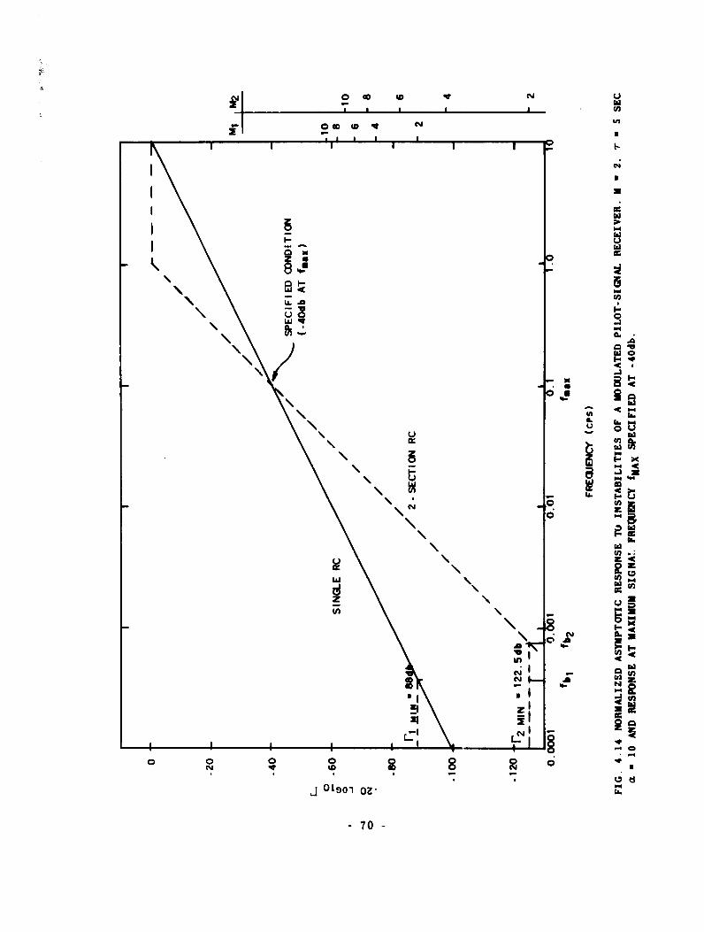
0 D 40Np p I p

\\ N

ow

-3

-- C

00-C

ALi I-

u

, 4c

chi

,LI".

N q I I - ,

IL o

04-0 0

detectable signal-modifying factor M depends on total noise power under

the smoothing-filter response, the AGC requirement depends on the tail

of the voltage response of the smoothing filter. In this case the ex-

tended response of the single section relative to that of the two-section

is an advantage.

The modulated pilot-signal receiver has the capability of equaling

the minimum detectable signal of a modulated signal receiver and has the

advantage that throughout the linear-response range of the receiver, the

improvement factor on instabilities remains constant. As was discussed

in Chapter III, and shown in Fig. 3.7, the slope of the calibration curve

is held constant but the zero point can change with changes in T.,.

4. Other AGC Systems

Two possibilities for applying AGC to receivers with modulated or

switched inputs are:

1. Connecting the servo loop to stabilize the receiver output for onestate while the signal is measured during the other state.

2. Connecting the servo loop to stabilize the receiver for one inputNtate while the signal is measured from the difference between thethe two states.

Time-sharing or switching techniques that isolate signal information from

the AGC channel will deteriorate the AT value.

A white noise that is square-wave gated does not change its spectral

character, although it does loose 3 db in strength. It undergoes an

irreversible process since aliased bands overlap, causing information to

be lost. The band-limited gain-instability noise can be sampled adequately

and detailed information of its waveform can be recovered. Consequently,

AGC voltages derived from switching systems will contain information on

the gain-instability fluctuations in the signal output, which can there-

fore be reduced, but they will not have information on receiver noise

fluctuations in the signal output. They do carry a similar noise fluc-

tuation which will add quadratically to the receiver-noise fluctuation

in the signal output.

An example of this type of receiver is shown in Fig. 3.2 which has

an M - 2. The factor C for instabilities will be equal to i/r, the

inverse of the AGC-loop gain.

When the signal output is derived from the difference between the

antenna and reference temperatures, and gated AGC is applied as shown in

- 71 -

Fig. 3.4, the effect of changes in gain and T*3 is opposite, that of a Dicke

system (see Fig. 3.3). The value of M will be

M * 2f1 + (TATer+7ref)]

and

- [(T-Tref)/(T+Ter)] (1/r)

This system improves the dynamic range over which instability eff.cta

are reduced compared with the Dicke system.

A process of further time sharing using three switch positions and

two reference temperatures as shown in Fig. 3.5 changes M even more, but

it results in a greater calibration stability. As shown neither gain nor

T., changes affect the calibration. Whether this three-position switch-

ing system can be achieved in practice without introducing undesirable

effects is not known.

In a critical application, an auxillary AGC loop might be in-

corporated, as shown in Fig. 3.6 to assure a constant detector operating

point. This additional AGC loop of course increases M even more. Each

stage in these stabilization processes must be justified in practice,

considering the many factors involved in a particular application.

Simplicity has many virtues as a design criterion.

- 72 -

V. RYLE AND VONBEBG TYPE RECEIVERS

4A. GENERAL DESCRIPTION

In previous chapters the null-balancing concept was introduced as a

means of stabilizing receiver calibration. The equipment described by

Ryle and Vonberg (Ref. 17) and later in more detail by Machin, Ryle and

Vonberg [Ref. 22) successfully demonstrated the method applied to radio-

astronomy measurements at meter wavelengths.

The necessary components required to perform the null balance con-

sist of:

1. A comparison device to indicate the difference or error between a

controllable reference source and the signal source.

2. An amplifier for the error voltage.

3. A controller for the reference source.

These components are connected to form a servo system that acts to null

the error voltage. Figure 5.1 illustrates such a system. Each of these

components will be discussed below with a viewpoint of presenting their

transfer functions and characteristics for inclusion in the servo loop.

1. Controllable Reference Sources

The basic requirement for the reference source is that its range

of variation coincide with the range of expected signal strengths. At

the same time a reliable measure of the reference-source strength must

be available for recording. Since the receiver will be designed for

particular measurements, the transfer function of the controlled source

must be satisfactory in terms of frequency response when ,-onsidered as

part of the servo loop.

Hyle and Vonberg used a saturated-noise diode whose filament

supply was readily variable. They chose to use lO-kc alternating current

supplied from a voltage-controlled source to heat the filament. A 350-

ohm anode load resistor was used which provided a 30,000 OK noise tempera-

ture (when transformed to the transmission line impedance of 70 ohms) at

an anode current of 15 ma. From their measurements the transfer function

for their diode was of the form Kd/(Td a +1), with Td - 0.09 sec during

heating and Td - 0.06 sec while cooling. To achieve stability in the

complete equipment, feedback proportional to the derivative of the anode

current was applied to the input of the control stage. The resulting

transfer function can be written in this form

- 73 -

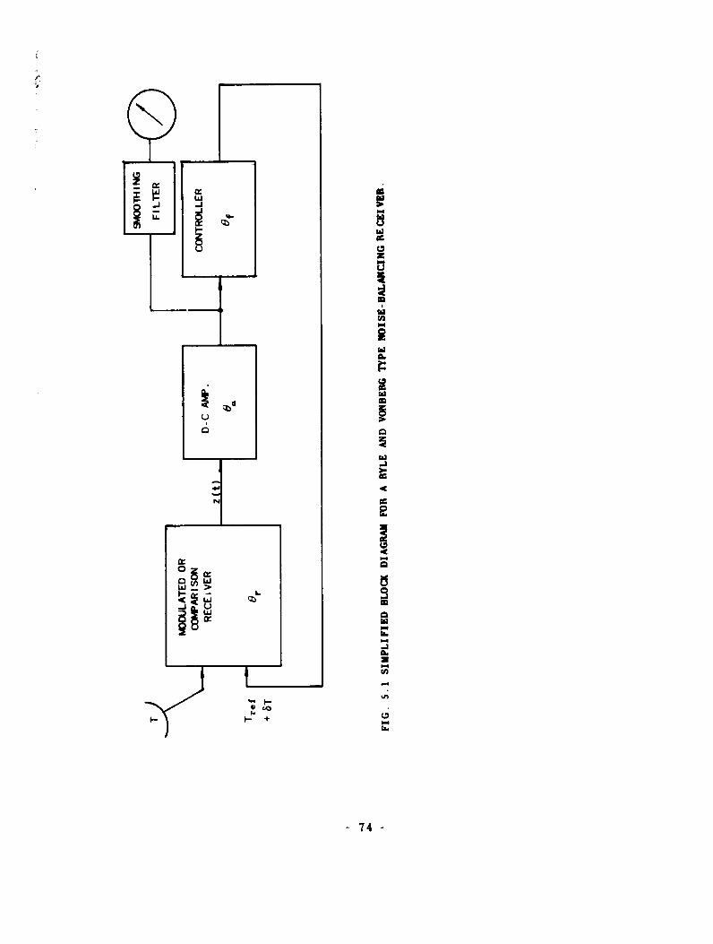
LL.

-J

w 1,

!i wj u

w01

3a

74

Kd(TO s + 1)

( 7 d a + l)(T,0 a + l) +K

where 7 0 isthe time constant of the feedback path.

A second convenient source of noise is a gas-discharge tube

coupled to a transmission line. The characteristics of such a source

are relatively independent of conditions of the discharge; hence, control

of the temperature to permit use of this tube as a reference source re-

quires the addition of a controllable attenuator. If the noise source

is in a waveguide a motor-positioned attenuator of the conventional kind

can easily be used. A simple scheme under some conditions is to utilize

a self-balancing, potentiometer-type recorder that has been modified

to move the recording pen and an attenuator card simultaneously for con-trol of the noise temperature. The measuring circuit must be disabled

also, so that the instrument operates as a servomechanism. When the

attenuator card is designed to give a linear temperature output as a

function of recorder-pen position, a very satisfactory means of control

and recording is achieved. One disadvantage of such a system is the

relatively slow response time of mechanical recorders and attenuators,

which limits the usefulness of the receiver to slowly varying signals.

The simplest transfer function of motor-driven attenuators will

be of the form K/s(TM a +1), which includes an integrating term 1/s

typical of motors and a time constant 7¥.

Another controllable attenuator is a resonant-absorplion ferrite

device with a variable magnetic field. A transfer function between a

fie.ld-coil current and noise temperature at the attenuator output could

be arranged with the form Kf/(f s + 1), with the time constant 7f de-

pendart on the L/H ratio of the coil and driving circuit. Although this

device cuuld be made with a satisfactory frequency response it still

suffers from an inherent nonlinear characteristic that would have to be

corrected either in the driving circuit or in the data reduction.

2. Error-Voltage Amplifiers

The main requirement for these amplifiers is sufficient gain.

Their noise level must, of course, be satisfactory and their frequencyresponse must be adequate. By making the frequency response of one stage

dominant, we can for our purposes describe the amplifier with a transfer

function such as K./( a + 1). The available output-voltage swing must

- 75 -

of course be large enough to drive the controlled noise source over its

full range.

3. Comparison Devices

Detecting a difference in temperature between two sources is the

fundamental operating prinr.iple for a Dicke-type receiver, and the logical

extension of this idea is the Ryle and Vonberg system. Therefore, we

shall consider Dicke-type receivers as comparison devices.

A requirement of rapid operation may result in a minimum of smooth-

ing within the comparison receiver itself; in fact, the determining element

in frequency response may be the video filter. The action of the coherent

demodulator translates the center of response of the video filter to zero

frequency, resulting in a low-pass response. A single tuned filter after

this operation has the transfer function K,/(T, a + 1).

Of course, when a smoothing filter is used at the ccmparison-

receiver output, the voltage-transfer function corresponding to the power-

transfer characteristic H(f) must be used to write the transfer function

for the comparison device. In the simplest case it would be the same as

the function shown above.

The discussion so far has not considered system noise. The com-

parison receiver will have a minimum detectable error signal as described

by the applicable AT expression. For our purposes we can assume that the

other components in the servo loop contribute no additional noise, so

that the loop noise output will be a modified version of that produced by

the comparison receiver. The details of the modification are presented

below.

B. NOISE ANALYSIS

For this study we shall assume that the system is balanced, so that

only small changes 87 in Tre f are present because of noise. Then ST has

a zero mean value and its mean-square value will be the total noise-power

output for the system.

For fluctuations from the mean for the closed loop we can write,

using the notation of Fig 5.1

ST (z - <z>) Oa Of - 'T Or 0& Of

z ( -'< i> ) 0 Of

I +Or 0a Of

- 76 -

• Now we use the relation between power spectral densities at the input

and output of a linear system to find the power spectral density for ST.

From Eq. (C. 11) the spectrum for (z -'<z>) is

C(f) - p, H(f),

where p3 is the uniform strength that is weighted by the filter response

H(f). Thus, letti.ng D(f) be the power spectral density for ST we have

D(f) - C (f) J Of0a Ofl)-Cl) + +O r 0' 0 t

We can then write

8 r ~ ~ aa 0 t*<Trei>.* T 1 9 ;~

and

S<Tref> (T' - T) Or e 6

I +Or 6 8 f

When A<Tref > a <ST , (T' - T) - AT the minimum detectable signal, by

definition, so that

AT . ,rT/ 0r(0) l+6r a f l-mo

Now

Or(O) - <z>/(T - Tre ) u Vp<z>H(O)/(T - Tre )

which can be evaluated from Eq. (C.8). The complete expression for AT

then, is

77 -

f G G It1 n c 1 ( 0 )J 2

2k 2 (Ter +Tro) 2eGG]o IK I2 f H( f) af/(1 +erOG.)I dfAT flum o -

(k2/4) f G(f)df 1/7) f /(t) (t)dt H(o)1.e0/(l+erOaOf)l-®D 0ffO

•M (Ter+Tref) 1/V7' Af,

where M is defined by Eq. (C.15) and

2

f/ 1(f) I980 0 f /(l + O 6 O(64)I df

II(0)IL) bf/(l+ 0o &aOf)I2

o & f=O

Since H(f) and 10r 12 are related by a frequency-independent factor, wecan rewrite the above equation as

16 e Of/(1 +a 6. )l2

f IOr Oa0 01' +& a Of)l 2 df

Fror the above analysis we see that the Ryle and Vonberg type receiver

depends on the behavior of the modulated-signal receiver used for comparison

or error indication. The minimum-detectable-signal expression is that for

the comparison receiver, except that the integrating time is modified by

the closed-loop transfer function

C. DYNAMIC BEHAVIOR

The transfer function for the receiver can contain an undetermined

number of poles and zeros, depending on the complexity of the individualcomponents. Two possible forms are those with a I/s term and those without.

Without the pole at the origin the device is a proportional-control system,

in which the error is reduced to as small a value as desired by providing

sufficient loop gain. This device then would have a fixed percentage

error but would always operate with a stable zero-signal point. Changes

78 -

in K, the loop gain, would result in calibration changes; however, for

large gains, the deviation from a unity proportionality factor would be

small, since the functional form for this factor is

K/( i +K) ^' 1 (K >> 1).

When a 1/s term is present the control system nulls with a zero error,

at which time excitation within the loop is noise only. The system re-

sponse will equal a step input signal after the decay of transients but

will have a fixed error for a given ramp-input signal. Errors are present

whenever the signal changes. The advantage of zero-steady-state error is

gained at the expense of more difficulty in stabilization of the control

system.

The general problem of describing control-system behavior in terms

of error coefficients has been discussed by Truxal (Ref. 23]. Figure 5.2

shows a single-loop system and the notation to be used for the discussion

of error coefficients: E(s) is the transform of the error signal, R(s)

is the transform of the input signal, and G(s) is the transfer function

of the forward path. The expression

E(s)/R(s) - 1/El +G(s)]

when expanded in a Maclauring series, can be written as

1/El +G(s)] [1/(1 +Kp)] +(s/K v ) + (s '.') + . . (11)

where the Ki are the error coefficients. When this series expansion is

a valid representation of E(s)/R(s) with only a few terms, then the

error coefficients have mean'ng as follows:

Kp is inversely proportional to an error depending directly on tiesignal

KV is inversely proportional to an error depending on the derivativeof the signal.

KA is inversely proportional to an error depending on the second de-rivative of the signal.

A more useful interpretation, from the viewpoint of radio astronomy,

is the relationship between the error coefficients and the noments of

79 -

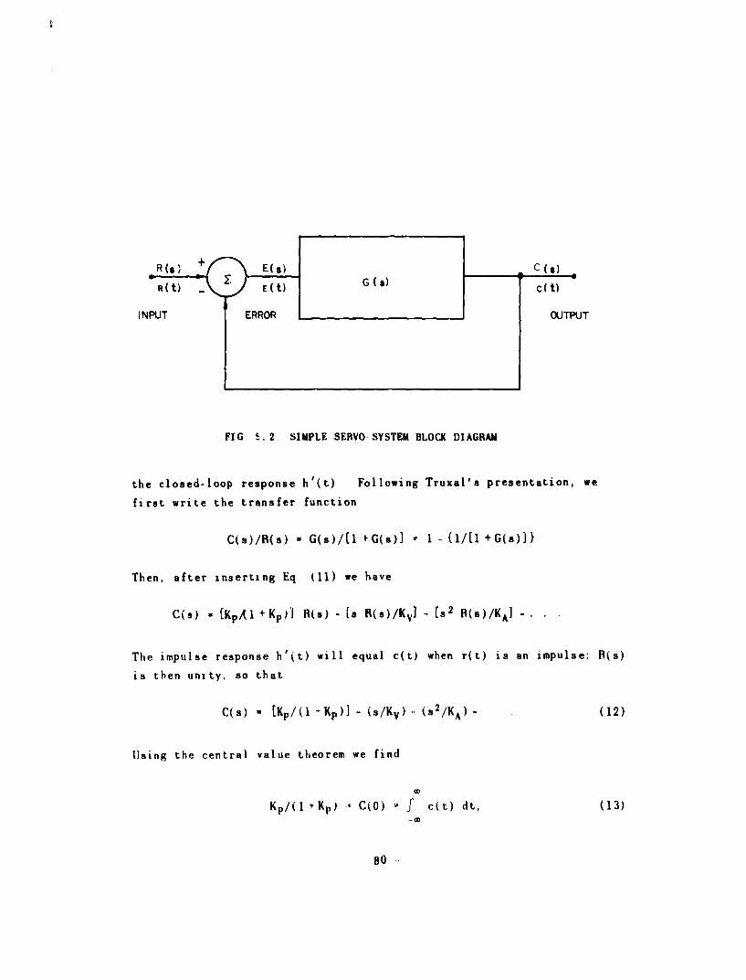
E ( t)_________________ OUTPUT

F1IG 5. 2 -SIMPLE SERVO- SYSTEM BLOCK DI AGRAM

the closed-loop response h'(t) Following Truxal's presentation, we

first write the transfer function

C(a) /H(s) - G(s)/(l f G(s)] -1 - l/l + G(s))}

Then, after inserting Eq (11) we have

C(s) - (KpAlI+ Kp)I H(s) - [s I(s)f/KyI - (2 Ht(s )/KAI-

The impulse response h'(t) will equal c(t) when r(t) is an impulse; H(s)

is then unity, so that

C s) - [Kp/ (1 Ki-)I - (s/Ky). (82 /KA) (12)

Using the central value theorem we find

KP /(I 4I(p) *C(O) fc(t) dt, (13)

80

which are expressions for the area under the impulse response. When Kp

is infinite the area is unity. Differentiation of Eq. (12) with respect

to a gives

C,'(s) - (Il/Kv ) - (2i/KA) -

From this we can write

I/Kv -C'(0) f t c(t) dt. (14)

Thus /KY s the first moment of the impulse response. A second dif-

ferentiation of Eq. (12) with respect to a gives

C"(s) *- (2/KA) -

From this we can writeS

I/KA -- CO (0)2 f. t2 c(t) dt,2 -0

which shows the relationship between KA and the second moment of the

impulse response. Similar relations exist for the higher-order moments.

In the next section, data-interpretation problems that can be dis-

cussed with the aid of impulse-function momenta will be presented. The

effect of variations of the moments of the impulse response can be re-

lated to the parameters of the control system or receiver through the

error coefficients.

D. LIMITATIONS

The performance of a Byle and Vonberg type receiver has been shown

to be excellent for the measurement of changes in input level. The

advanitages of the modulated-signal receiver regarding zero-point stabili-

zation are achieved over the whole range of measurement with no further

increase in the minimum detectable signal. The usable integration time

is usually set by some observational requirement, so that the effect of

the control loop can be included in the original design to insure the

desired value for r.

The question of integration time, however, does bring out two features

of the Byle and Vonberg system that must be considered. First, inasmuch

- 81 -

as the loop desigr is an important factor in determining T, a difficulty

arises in regard to readily changing T for different measurements

Second, the value of T that results from a given design is dependent on

loop gain. Here then is a characteristic of the receiver that does de.

pend on gain stability.

Up to now the input to the receiver has been considered at a constant

level. however, in the discussion of the Fyle and Vonberg type receiver.

the behavior with more general signals is an essential consideration

When a source passes through the antenna pattern, the receiver output

has a time-varying level. Th-s output has a band-limited waveform and

differs from the true representation of the source distribution because

of antenna smoothing and smoothing in the receiver The effects of re--

ceiver smoothing will be considered below In Fig 5. 3 a typical source

observation is presented in terms of spectra and waveforms

The details of the source distribution have to be determined from

the receiver output, with such things as position, angular extent, and

total flux of interest Let us consider position measurements The

position of a signal in time can be described by the time coordinate of

its centroid t defined as

t * f t z(t) dt/f z(t) dt

relative to an arbitrary zero The operation of smoothing produces a

shift in the abscissa of the centroid, depending on the smoothing function

This process can be des7ribed by the following theorem, which is proved

in Appendix D

THEOREM The centroid of the signal waveform will be located t h secin time before the centroid of the recorded waveform where th is thetime coordinate of the centroid of the impulse response of the receiver in relation to its origin or time of impulse.

Using error coefficients, we can write

t h ' (1 + Kp)/KpKv

which displays the need for error- coefficient stability if position

measurements are to be accurately made The fractional change in t,

82

BEAM PATTERN SPECTRAL SENSITIVITY FUN4CTION

0 t f

SOURCE SMDOTHED BY ANTENNA SMDOTHED SOURCE SPECTfRUM

tot0 f

RECEIVER IMPFULSE RESPONSE RECEIVER Sh)OTHING SPECTRUM

O t 0 f

RECEIVER OUTPUT SPECTRUMd OF RECEIVER SIGNAL OUTPUT

FIG. 5.3 SPECTRA AND TIME FUNCTIO1S SHOWING THE TWO SMOOTHING OPERATIONS

OCCURING DURING THE OBSERVATION OF A DISCRETE SOURCE.

-83 -

relative to a fractional change in loop gain K can be defined as SK, an

important measure of sensitivity to this effect. Thus

SK - (d th/dK) (K/th ) (16)

This expression can be evaluated for systems as shown in Fig. 5.2, let-

ting G(s) . K F(s), where K is the loop gain factor. Then

C(s) - K F(s)/[l +K F(s)]

C(O) - [K F(0)]/[l +K F(O)]

C'(s) - [K F'(s)]/[l +F K(s)]2

and

C'(O) • [K F'(O)]/[l +K F(O)]2

Then, from Eqs. (13), (14) and (15), we can write

th a " C'(O)/C(O)

- F'(O)/F(O)dl +K F(O)]

The derivative of th with respect to K,

dth/dK - F'(O)/(l +K F(O)] 2

Now, substituting into Eq. (16), we have

s -K F(O)/[l +K F(O)]

- C(O)

Since the null.balancing principle requires C(O) the d-c gain, to be

very nearly unity, SK will be the same for any configuration of components

in the system.

A general statement for Hyle and Vonberg type receivers is that the

accuracy of position measurement depends directly on loop-gain stability,

- 84 -

with a 10-percent change in loop gain giving a l0-percent change in the

position correction to be applied to account for the receiver smoothing.

Attempts to reduce the absolute error by using smoothing functions

with small first moments and hence small tbs, will lead to other dif-

ficulties associated with negative responses and longer times in which

noise can introduce errors.

E. SUPPLEMENTARY SMOOTHING FILTEBS

By designing rapid response into the receiver, so that the effective

integrating time is short compared with those desired for measurement,

it is possible to further amootA the output with a filter of the desired

characteristics. This supplemental filter can be chosen to be stable

and, since it provides the majority of the integration, gain changes do

not cause trouble. A second feature is the improved ability to change

integration times and smoothing characteristics readily without disturb-

ing the receiver dynamic performance. When special complex smoothing

functions are desired, operating on the signal outside the loop is a

distinct advantage.

The device which provides the reference noise source will determine

the manner in which it is possible to obtain an output signal for further

supplementary smoothing. What is advantageous in general is to have no

active element subject to instabilities between the signal output and

the actual noise-level reference. In the case of the noise diode, the

indication of noise is directly and simply related to the noise level

and at the same time is an electrical signal that lends itself to sup-

plementary smoothing. The difficulty with the noise diode is the inherent

thermal delay in the heater, which may prevent one from achieving very

small integrating times.

A ferrite attenuator designed with a linear relationship between

noise level and driving signal would be capable of rapid response and

have the electrical signal for further smoothing. This attenuator seems

to be a desirable controller for the reference noise source.

85 -

VI. STANFORD MICROWAVE-SPECTROHELIOGRAPH RECEIVER

A. GENERAL REQUIREMENTS

The Stanford microwave-spectroheliograph antenna, described by

Bracewell and Swarup [Ref. 241, is a pencil-beam interferometer composed

of two, perpendicular, 16-element arrays, phase-switched together to form

the multiple pencil beams. The arrays operate between 2700 and 3400 Mc,

providing at 3292.1 Mc a half-power beamwidth of 2.3 min by 2.3 deg.

Pencil-beams 3.1 by 3.1 min are formed by the complete antenna and, for

solar observations, raster scanning is performed so that contour maps

of solar-brightness temperature are obtained. Patrol observations on the

sun using the east west array provide one-dimensional scans of brightness

every 3 to 5 min over an 8-hr period. Automatic-control equipment for

the antenna allows patrol observations to proceed unattended.

The collecting area of the antenna and the transmission-system loss

are such that equivalent input temperatures for the receiver will vary

from about 200 OK (for cold-sky observation) to several thousands of

degrees.

1. Bandwidth and Beamwidth Belationship

Because the antenna is a multiple-element interferometer, the

reception-filter bandwidth must be limited if a narrow beam is to be

maintained in directions making a large angle q as measured from a plane

perpendicular to the array. The nature of this beam broadening due to

receiver bandwidth can be understood as follows. The field originating

in a source with a flat power spectrum (or nearly so) in the frequency

range of interest and incident on the antenna can be described over

periods smaller than the reciprocal reception-filter bandwidth by a

single frequency and amplitude of oscillation During such an interval

the antenna pattern is that given by monochromatic theory and an output

contribution is produced from a point source according to its position

relative to the particular monochromatic beam formed. Over long periods

the detected power spectrum from the source is related to the power-

transfer characteristic G(f) of the receiver. Each frequency bf, de-

fined as f- fo, produces a beam at a different angle around q0 defined

by the central frequency fo and an order-of.-interference number m. We

have

sin q0 mX/d - m c/d f

86

and

Sqo " m c Sf/d(cos qo) f!

The distribution of beams around q. is weighted according to the function

G(8f) expressed in terms of 8q using the relation above. If we call

this G(8q) and use the antenna response aroung q. (Bef. 25]

P(q) -sin V7Td(cos q)Sq/h

(7d/X)(cos qo)6q

the effect of bandwidth broadening is described by the relation

P'(Sq) - P(8q) * G(Sq) (17)

This convolution of the two functions describes the way in which the

various contributions from different frequencies are combined to pro-

duce a resultant beam P'(Sq). Instead of using the half-power width

of both P(8q) and G(Sq) as parameters, once can achieve an advantage by

introducing the ratio of the half-power width of G(Sq), wG,1/ 2, to O€

the peculiar interval for the antenna. Since both of these functions

vary with q, their ratio

- = 16 K In bf/f

where

K 1 for the cross

2 for an array

and where Sf is the half-.power width of G(f). Equation (17) has been

solved numerically to obtain the resultant beam half-power width These

rcsults appear in Fig. 6.1 for a single array and the cross with both a

rectangular and a single-tuned-response form for G(f). The single-tuned

The peculiar interval 4 a X/16d cos q for the cross and X/32d cos q for a singlearray and is the reciprbcal of twice the highest spatial frequency to which theantenna responds.

87 -

3.0

SINC 2 -A,

2.5 --- - -

SINC2 *

-*I-

-

3

2.0

• /0.

SINC A/// ¢

1.5 . ///

/SINC On1

0 0.4 0.8 1.2 1..6 2 2.4 2.8 3.2 3.6 4 4.4 4.8

Rt = WG. V/,k

FIG 6. 1 RELATIVE BEAM BROADENING DUE TO CONVOLUTION WITH RECTANGULARAND SINGLE TUNED CIRCUIT POWER RESPONSE FUNCTIONS.

88 -

response results in a wider beam than the rectangular response. The

theoretical half-power beamwidths for a single array and the cross have

been plotted in Figs. 6.2 and 6.3 including the 1/cos qo factor. Several

reception-filter widths available in the receiver are shown to indicate

the expected beamwidth for hig-order interference numbers. For solar

mapping with the cross, use of the 0.5-Mc bandwidth out to the m - 20

response results in less than 5 percent broadening and less than 10 per-

cent broadening out to the m a 30 response.

2. Temporal Besvonse of Beceiver

The temporal response of the receiver as limited by the smoothing

filter must be fast enough so that source-distribution information is not

lost during scanning observations. The maximum-frequency component at

the output of the receiver related to the source distribution is determined

by the upper limit of the spectral-sensitivity function (SSF) for the

radiotelescope and the scanning rate. If sh is the highest spatial fre-

quency in the SSF in cycles/radian and the scanning rate is 0 radians/sec,

the highest frequency out of the receiver will be

fh a sh

For the cross, fh is 0.0488 cps and for the east-west array, 0.0976 cpswith the earth's rotation. Consequently, the frequency and phase re-

sponse of the smoothing filter at these frequencies must be such as to

produce negligible distortion. The sampling theorem applied to the above

outputs requires samples every 10.2 sec and 5.1 sec respectively.

3. Accuracy

The bandwidth and response-time requirements given above lead to

a minimum level.-uncertainty figure UL for the radiotelescope. Allowing

an integrating time (-r) of 0.5 Mc, we obtain

UL - l/v/l - 0,63 x 10"3

If we set a limit of 1 percent accuracy on measurements a 1-percent change

in temperature should be detectable. For the 200 0 K-sky case, this means

a 2 OK minimum detectable signal. The product of modifying factor M and

system equivalent noise temperature then must be given by the basic

equation (rearranged)

89-

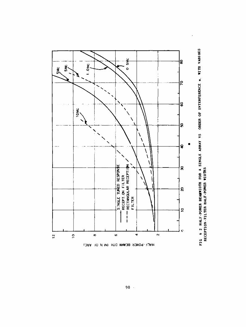
u

U Ln

u U

u -

19I

- _ _ _ _ - -cc

0c

-- -- --- --- - - ____ Uto

-H

CLCr I-

w a.

-- J ir l1

00

~ J~L 28 83~dA16

900

4C

in0

z

0 waa.

00cc

* _ _ O_

(08V~~ ~ ~ ~ ~ JO NIOI-OMNV 3~dA

90'1:

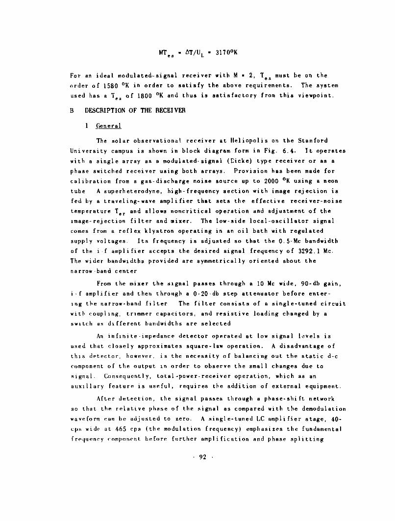
MT -AT/U - 3170OK

For an ideal modulated-signal receiver with M - 2, Tes must be on the

order of 1580 OK in order to satisfy the above requirements. The system

used has a Tes of 1800 OK and thus is satisfactory from this viewpoint.

B DESCRIPTION OF THE RECEIVER

1 General

The solar observational receiver at leliopolis on the Stanford

University campus is shown in block diagram form in Fig. 6.4. It operates

with a single array as a modulated-signal (Eicke) type receiver or as a

phase switched receiver using both arrays. Provision has been made for

calibration from a gas-discharge noise source up to 2000 OK using a neon

tube A superheterodyne, high-frequency section with image rejection is

fed by a traveling-wave amplifier that sets the effective receiver-noise

temperature Ter and allows noncritical operation and adjustment of the

image-rejection filter and mixer. The low-side local-oscillator signal

comes from a reflex klystron operating in an oil bath with regulated

supply voltages. Its frequency is adjusted so that the 0.5-Mc bandwidth

of the i-f amplifier accepts the desired signal frequency of 3292.1 Mc.

The wider bandwidths provided are symmetrically oriented about the

narrow-band center

From the mixer the signal passes through a 10-Mc wide, 90-db gain,

i-f amplifier and then through a 0-20-db step attenuator before enter-

ing the narrow-band filter The filter consists of a single-tuned circuit

witt coupling, trimmer capacitors, and resistive loading changed by a

switch as different bandwidths are selected

An infinite-impedance detector operated at low signal levels is

used that closely approximates square-law operation. A disadvantage of

this detector, however, is the necessity of balancing out the static d-c

component of the output in order to observe the small changes due to

signal. Consequently, total-power-receiver operation, which as an

auxillary feature is useful, requires the addition of external equipment.

After detection, the signal passes through a phase-shift network

so that the relative phase of the signal as compared with the demodulation

waveform can be adjusted to zero. A single-tuned LC amplifier stage, 40-

cps wide at 465 cps (the modulation frequency) emphasizes the fundamental

frequency (omponent before further amplification and phase splitting

92

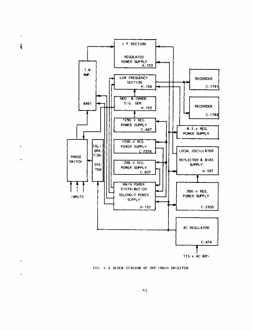
I F SECTION

REGULATEDPOWER SUPPLY

H - 103-T.W.

AMP .

LAl OW FERQUPPLY RORBRAT

PHASECTION

SF

W FREI

MAIN5 POWERDE

E25~BUO -50- REG.G

INPUS SOENOD POER OWER SUPPLY

SUPPLYPPL

C_ 2 3653

SWITCH__4-_E -________VREG __REFLCTREG &LATOR

C1-

ACI&

SYS- 6 OWE SUAPPLY OFSUPCOPLYCEV

TEM C-67 H-10

occurs The gain through this section is adjustable in two decades of

nominal values ti e , 0, 10, 20, .., 100 and 100, 200. 300, _1000)

The coherent demodulator accepts a balanced-signal input that is

transmitted or shunted to ground depending on the state of two pairs of

triodes connected back to back. The balanced demodulation input square

wave drives the common grids of each pair to provide the switching action.

The single ended output feeds the smoothing filter, which is a single

section RC low-pass network loaded only by a cathode follower A second

cathode follower with an adjustable grid voltage provides a zero balance

control for the potentiometer type recorder connected between the :athodes.

An adjustment of recorder deflection is provided with a continuous

control followed by an accurate step potentiometer with 1.5 db steps of

voltage into the 100 0 - 100 my recorder

2 Input Circuitry

Two types of observation performed at Heliopolis are the one-

dimensional scanning obtained from a single array and the two-dimensional

scanning obtained by phase switching the two arrays.

An input system has been developed that allows both of these ob-

servations to be performed with only a simple change in input waveguides

For phase-switched operation, the waveguide transmission lines from the

two arrays terminate at a cnlinear pair of ports of a matched -hybrid-tee

junction One of the side ports will provide the sum of the voltages

from the two arrays and the other port will provide the difference Now

if the phase length of one of the array signal paths is changed by 180

deg, the outputs of the two side ports will be exchanged. Thus, at either

side port, the signal changes from a sum Lo a difference or vice-versa

when the phase length of one input is changed by 180 deg The input

circuit is diagrammed itt Fig. 6 5

A two-port device whose phase length changes by the required 180

deg at a frequency of 465 cps is the key component The design and con-

struction of this device using varactor diodes resulted in an efficient

and reliable phase switch that is readily driven at 465 cps and that is

capable of operation at much higher frequencies

The input and output of the variable-phase element are the colinear

ports of a matched, hybrid tee junction The side ports are connected to

shorted sections of waveguide, each containing a varactor diode When

these sections are properly adiusted for one condition of the diodes

94 -

wx

w

L&JL

0

w~

cU,

ZLJ -

cr-95-

the signal that enters the hybrid junction is divided between the two

side arms, is reflected after traveling a certain phase length, and is

then recombined in proper phase to proceed through the output port. When

the diodes are in the opposite bias condition, the shorted sections

appear a quarter-wavelength longer and hence a total phase length of 180

deg is added to the signal.

With careful construction and adjustment of the switch, the simul-

taneous amplitude modulation is negligible and the insertion loss less

than 0.8 db Since the variable phase element appears in one input line

only, the switch-insertion loss in db is effectively only one half that

of the element itself. A detailed description of the side-port shorting

sections shown in Fig. 6.6 is given in Appendix E.

When single-.array operation is desired, a waveguide section as

shown in Fig 6.7 is connected to the phase-switch inputs. The additional

matched hybrid tee junction provides sum and difference outputs composed

of antenna and reference source contributions. The action of the phase

switch on these inputs is to yield either the antenna contribution or the

reference-source contribution at the output for the two phase switch con-

ditions The result is a switching of the receiver input between the

antenna and the reference source and consequently square-wave modulation

of the antenna signal

Included in the input circuitry shown in Fig. 6.5 is the calibration

system A high-directivity, 10.db, directional coupler is inserted in

each input and these are fed from a single gas-discharge noise source

whose output is attenuated and divided by a matched- hybrid-tee junction.

This hybrid junction is important because it gives additional isolation

between inputs for any signal which tends to couple through the cali

bration system When properly connected, the known calibration signal

from the noise source appears at the traveling-wave tube input in proper

phase to provide the same-polarity output deflection as the antenna sig

nal when the microwave switch configuration is in use.

3 H-F and I-F Sections

The output of the phase switch is connected to the traveling-wave

amplifier through an isolator to minimize any effects of impedance modu-

lation produced by the phase switch An RCA 6861 low-noise traveling-

wave tube (TWT) provides 23 db of gain with an effective noise temperature

of 1200 OK This tube has given excellent service, being in continuous

operation for over 20,000 hr The operating voltages for the TWT are

-. 96 -

0:0

u+ z

R 0 -4- a

z

2.. 5 F ) -IV

04

u C?0

(-I

UJ 0 0Ln V-

OD)

l,

00LLU,

cc

crzLLI C

ui Cal

J0 0..

(7) Ln C r L

~~u cn U'F-0

Go u 0

Ca.

97

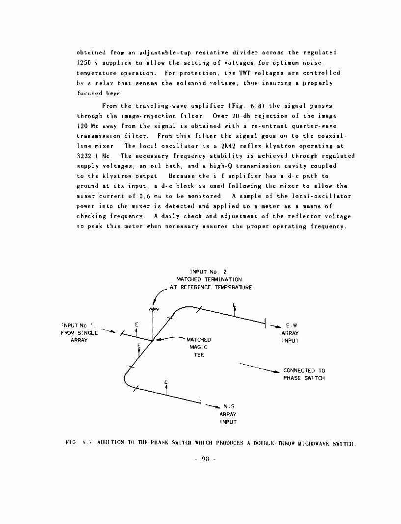
obtained from an adjustable-tap resistive divider across the regulated

1250 v supplies to allow the setting of voltages for optimum noise-

temperature operation. For protection, the TWT voltages are controlled

by a relay that senses the solenoid ",oltage, thus insuring a properly

focused beam

From the traveling-wave amplifier (Fig. 6.8) the signal passes

through the image-rejection filter. Over 20-db rejection of the image

120 Mc away from the signal is obtained with a re-entrant quarter-wave

transmission filter. From this filter the signal goes on to the coaxial-

line mixer The local oscillator is a 2K42 reflex klystron operating at

3232 1 Mc. The necessary frequency stability is achieved through regulated

supply voltages, an oil bath, and a high-Q transmission cavity coupled

to the klystron output Because the i f arplifier has a d-c path to

ground at its input, a d-c hlock is used following the mixer to allow the

mixer current of 0.6 ma to be monitored A sample of the local-oscillator

power into the mixer is detected and applied to a meter as a means of

checking frequency. A daily check and adjustment of the reflector voltage

to peak this meter when necessary assures the proper operating frequency.

INPUT No. 2MATCHED TERMINATION

AT REFERENCE TEMPERATURE

NPUT No 1 -s E WFROM SNGLE I/ARRAY

ARRAY ----- MATCED INPUT/M M~TEE.

CONNECTED TO

PHASE SWITCH

ARRAYINPUT

FIG 0.7 ADI)ITION I) TIIE PIIASE SWIT(1 WIllICII PIRODUCES A DOUBL - tIIIIOW MICI )WAVE SWITCII,

- 98 -

U

V CL.)

0 0

a (L U c

-o 0 Cfl

0 R 0

V 00

Q'a.

V) LJ U

>J4 0 )

> - nU~~ t3Mn ccN3

Cz(

99

The 60..Mc i-f amplifier is an unmodified commercial unit with

10-Mc bandwidth and is normally operated at maximum gain. The attenuator

following the i-f amplifier has a range of 0 to 20 db in l-db steps and

is useful for performance checks as well as providing i-f gain control.

Because of bandwidth effects on the antenna pattern as discussed

above, a range of bandwidths (0.5, 2.5, 5, and 10 Mc) is provided. The

i-f amplifier output at a 10..Mc bandwidth is coupled into a single-tuned

circuit adjusted to the desired 3-db bandwidth through resistive loading.

A bandswitch changes coupling, trimming capacitors, and loading resistors

as necessary. A cathode follower transfers the signal from this filter

circuit to the detector.

4. Detector and Low-Frequency Section

The receiver depends on square-law detection for proper operation.

The infinite-,mpedance detector circuit, when operated with small sig-

nals, has a satisfactory square-law response, as demonstrated by the

graph of Fig. 6.9, which is an over-all calibration-response curve for

the receiver from input to output and has less than 1-percent rms error

as measured from a best-fit straight line.

100

N 80-J

60=

w 4~ 0

w

~ 0

IL 2

200 400 600 Boo 1000

INPUT TEMPERATURE(°K)

FIG. 6.9 POWER RESPONSE CURVE FOR THE COMPLETE RECEIVER. THE R MS

DEPARTURE FROM A STRAIGHT LINE IS LESS THAN 1 PERCENT.

100 -

After detection, as shown in Fig. 6.10, the signal passes through

a variable-phase-shift network which is set for maximum receiver output

with a standard calibration signal. With the square-wave modulating-

waveform generator used, no adjustment of the phase of the demodulating

waveform can be made; hence this must be done in the signal channel.

A single-tuned LC amplifier follows the phase shifter with a band-

width of 40 cps. This filtering sufficiently reduces the noise power

that must be handled by the low-frequency amplifiers and coherent de-

modulator to avoid saturation problems on noise peaks. The bandwidth is

not so narrow, however, that slight frequency drifts of the modulating..

signal generator result in undue phase shifts and consequent output

fluctuations.

Forther amplification is provided by two RC-coupled stages. These

have voltage dividers providing a range of gains from 10 through 1000.

The coherent demodulator requires a balanced input which is obtained with

a phase-splitting circuit.

S. Demodulation and Output Sections

The coherent demodulator is a realization of the switching circuit

shown in Fig. 6.11(a) by the vacuum-tube circuit (b). For zero input

the d-c output is but a few millivolts and stable, so that satisfactory

compensation can be made with the zero set control of the cathode-follower

pair driving the recorder. The output impedance for the dexodulator is

high, so that the smoothing filter must necessaril/ also be high impedance

and require the use of cathode followers to drive recorders and output

meters satisfactorily.

The smoothing filters provided have the characteristics shown

with the cirLuit diagram in Fig. 6.12 The recorder used may add a sub-

stantial amount of smoothing so that observations made where there is a

question as to smoothing effects should include specific measurements

for determining the over-all. smoothing present. Impulse-response checks

or frequency-response measurements may both prove of value in such cases.

The cathode followers mentioned above are connected as shown in

the schematic in Fig. 6.13. Both impedance-matching and zero-set func-

tions are present in this circuit. A mercury cell furnishes the grid

This circuit is an adaptation of one originating in the Radipphysics section ofC.S.I.R.O. Sydney, Australia.

- 101 -

00

0.

I__ _ _ I r.

z

a:aLL-

I'w

IL UjIn

CL a.

Tww~10 -rc

(a) SWITCHING-CIRCUIT REPRESENTATION

50kIM 2. 2M

SIGNALDEMOD.IN Tf~lI N

12AU7 103

I-J0i

104

voltage for zero setting with a lifetime of about 60 days. In normal

operation, a 100 0-100 microammeter and two 100-0--100-mv recorders are

operated in parallel between the cathodes.

One recorder has a slow chart speed (1.5 in./hr) for use as a

log of receiver operation. The second recorder produces the analog out-

put of observations and has an adjustable attenuator for calibration and

standardization of records. A continuous potentiometer followed by an

accurate step potentiometer makes up this attenuator. Since the self-

balancing-potentiometer, recorder-input impedance at balance is very

high, loading of the final attenuator is very small and its accuracy

is maintained.

6. Auxiliary Apparatus

Power is supplied from the 115-v 60-cycle lines through an elec-

tronic regulator that furnishes a constant rms value of voltage. The

receiver has regulated d-c supplies for 650, -500, -250, -6.3, and +250v.

+250

1 2AU7

I 1.34v

IN 2 1k

(FROM8%OTH I NGFILTER) 05iFITE)6 8k 6 r ° 8k 47k

C

B

A

AN 3102A16- lOS

FIG. 6.13 CATHOI)E-FOLLOWEIi OUTPUT CIRCUIT

1.05 -

Of these, the -650 and -500 v supplies are used for the local-oscillator

reflector and beam voltages respectively. Several critical circuits

operate better wit; d c heater power so this has been provided from

transistorized regulated supplies. Vhile a single supply would have been

satisfactory, the course of construction and developement led to smaller

separate units The TWT has d c heater power as well as the i-f amplifier,

filter, and detector circuit, and also the tuned 465-cps amplifier,

demGdulator, and output cathode followers.

The TWT solenoid requires 110 v d-c at 1.5 a. Heating of the

solenoid produces a large change in resistance, hence, during warm-up,

the proper current must be maintained by changing an adjustable trans-

former feeding the rectifier filter comgination.

A separate +250-v regulated supply is used for the modulating anddemodulating signal generator to prevent these signals from appearing

throughout the receiver on the +250-v bus. The blocks enclosed by the

dashed line in Fig. 6.10 are the circuits so supplied. In order to

generate square-waves without problems in asymmetry the scheme shown is

employed. An R-C phase-shift oscillator at twice the desired frequency

feeds a Schmidt trigger circuit adjusted to trigger on positive-going

zero crossings. The resulting rectangular waveform is differentiated

and clipped to provide a twice-frequency trigger pulse. When this wave-

form drives a bi-stable multivibrator a square.waveoutput is producedat the desired frequency. Various phase splitters, cathode followers,

and reference diode clippers provide all the necessary output waveforms.

From the square-wave at 465 cps, a tuned amplifier selects the funda-

mental component for a somewhat distorted sine-wave output.

Several test points are brought to the front panel through a

selector switch so that waveforms can be monitored easily. These appear

on positions of the test function switch: No. I (not used) No. 2,

detector output, Nos. 3 and 4, two phases of the demodulating waveform,

No. 5, one signal input to the demodulator, No. 6, the output of the

demodulator.

C CHARACTEISTICS AND PERFOR11ANCE

1. Critical Features

The [WT must be properly adjusted for lowest effective noise

temperature and adequate gain This adjustment results in a stable

condition and requires little further care. Proper image rejection is

- 106 -

necessary to prevent simultaneous reception from two interference maxima

at different positions in the sky resulting from the two bands. A min-

imum value of 20-db rejection is maintained.

The departure from ideal square-law detection has to be small

bat is readily measured and is repeatedly checked during calibration pro-

cedures. For a detector response with linear as well as a squared term,

the departure from the best-fit square law can be shown to be linearly

related to the linear-term coefficient and also to the range of input

signals considered. Thus, for small ranges of input and a small linear

coefficient, the approximation to square law operation is sufficiently

accurate. When operated to keep the active sun response well on scale,

inputs to over twice full scale remain on a linear portion of the system

and do not show the effects of saturation.

The stability of the gain and the bandwidth is an important con-

sideration. Although the modulated-signal mode of operation giver a

considerable improvement factor for output fluctuations due to instabil-

ities, their effect is present and must be responsible for the majority

of the difference between actual and theoretical minimum-detectable-

signal values.

Phase switching in practice has a tendancy to introduce losses,

unwanted responses, and inefficient operation. There may be a fixed loss

for signals passing through the phase-reversing element. Half of this

is the effective loss for the switch, since only half the signal passes

through it. If the phase reversal is not complete, the output is less

than optimum. For symmetrical untennas, with a difference,*' between

180 deg and the actual shift in phase the output is reduced according to

the equation

P - P,,X cos.€/2,

where P.sX is the maximum output fortk equal to zero and provided

optimum phase-length compensation is introduced into one transmission

line. For unsymmetrical antennas, the pattern is affected as well as

the amplitude [Ref. 251.

In addition to a fixed loss, the switch may have a variable

transmission efficiency. This shows up as an amplitude modulation at

fm superimposed on the phase-reversal modulation. The effect of thisamplitude modulation is most deleterious when a solar observation is

107

made with the cross and a large source is in one array response and not

the other. Such a condition can lead to the presence of a spurious fan.

beam-response record supcrimposed on the cross record. These responses

have to be held to a small value even with the extreme differences in

array response possible from the active sun. Because of this, phase-

switch adjustment is carried out to minimize amplitude modulation even

at the expense of poor efficiency resulting from incomplete phase re-versal. Fortunately, the loss for a small .i is not serious. A ferrite

isolator between the phase switch and the TWT also help to minimize the

amplitude-modulation effects.

2. Minimum Detectable Signal

The measurement of AT was made with the aid of a digitizer and

printer. A series of digitized values of the output for a zero-signal

condition was recorded, followed by a series after the introduction of a

calibration step. From this data, the mean value of the level on each

side of the calibration step was determined. Then the actual calibration

slope in divisions per OK was obtained. Following this, the standard

deviation from the mean was calculated for both levels. Two values of

A6T were thus obtained from this process.

With the following parameters for the receiver:

T - 1800 OKes

M - 7/V2

T - 2.67 sec

Af 1.57 x10 6

the theoretical value for AT is 1.95 K. Using a calibration step of

16 °K, values of 2.44, 2.52, 2.43, and 2.36 OK were deduced from measure-

ments. These values yield an average value of 2.43 OK for the experimental

minimum-detectable signal.

13 SAMPLE RECORDS

1 Fan-Beam Solar Record

The repeated solar scans which the antenna provides from the E-W

array while tracking are used as a patrol on solar activity. The record

- 108

in the absence of activity repeats with very little change from scan to

scan, as can be seen from the record reproduced in Fig. 6.14.

2. Pancil-Roan Solar Records

When the antenna is operated as a cross, the successive scans

appear with opposite polarity and exhibit great differences as the pencil-

beam scans different portions of the sun. Such a record is reproduced

in Fig. 6.15.

3. Weak-Source Record

As a contrast to the large signal-to-noise ratio of the solar

records, a fan-beam observation of the moon's thermal emission is shown

in Fig. 6.16.

10 APRIL 1961

18h 3 3' 145 18h 3 a q5

IGT 1S PREC EFSMICROWAVE BURST IS PRESENT.

The solar observations have been reported by Swarup (Refs. 25,25].

- 109 -

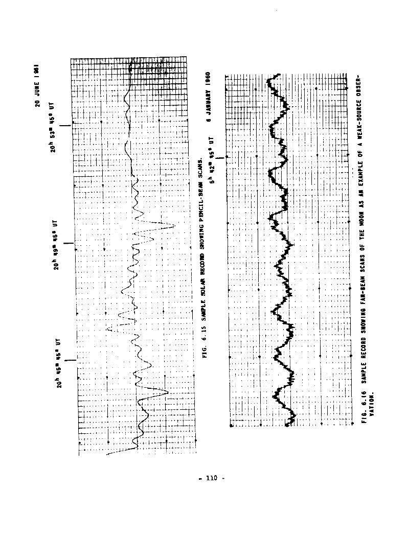
'.4 3W7

..................... ...... .. 63. 1 l I . -

.C .. ... . . . . . . . . . . . . . . . . . . . ....................

,~~~I ...f~ '****~*

.. .. . . . ... . . ..

... ... ..... l

(.4

110<.

VII CONCLUSIONS

A. SUMMARY

For all the types of stabilized receivers discussed, the attempts to

gain freedom from instability problems result in greater minimum detect-

able signals Other methods of improving signal to noise ratios such

as repeated measurements or simultaneous observations are demanding with

respect to time or equipment and furthermore depend upon the randomness

of the noise from measurement to measurement in order that a

l/'No of measurements improvement factor can be achieved. When a maximum

- and Af is reached, instabilities are controlled and the system noise

temperature is a minimum without yielding a small enough AT, these multi-

measurement techniques can be applied.

The properties of several receivers relative to a total power re-

ceiver are shown in Table 7.1 Although this tabulation is an aid in

determining the choice of a type of receiver, still, the estimation of

the cost and effort required to achieve a certain stability with a re-

ceiver in a given application must remain as part of the design problem

in which experience is most helpful

Various receivers have been considered in relation to the effect of

instabilities on their calibration curves. From this viewpoint we see

that constant zero signal output in the presence of instabilities is

achieved by most stabilized receivers including the d-c comparison,

correlation, Dicke, and Byle and Vonberg types The modulated pilot

AGC receiver achieves this for gain changes but not for T,,s changes.

The calibration curve behavior for large signals in the presence of

instabilities as shown in Table 7.1 for the Hyle and VontFrg receiver is

independent of gain and Tes changes and the slope of the calibration curve

is maintained constant For the modulated pilot AGC receiver this is

true except that Ta changes shift the zero signal output level.

The M value of V2 for the d-c comparison and correlation receivers

is low but it is achieved at the expense of dual channels. The cor-

relation receiver with circulators and cooled terminations holds the

promise of being a good wide-band receiver

For modulated signal receivers the M value of 2 remains quite theo-

retical since in piactice a video filter is usually used with the re-

suiting M factor of n//2 or 2 22 for the optimum square-wave modulation.

111

0

.0.

to v

I-

v ILI 0

6. 4.

W4~~~ .0 t, -a06 ~ ~~ 0 05 I. 6 1 6 - 1 V 6

U ~ ~ 6 1.- -* .4416

- - __ ___ 1 UU +

It CA

a 41 6Ir_

6 ~~ .JN.6~1

* .a a 6 .~ 4 *- .- 6z N 4)~ 60. 6 a40a

6... 6 1 k6... ~ 6 6 0 I r

6 ~ ~ ~ ~ : 6 41 * 6 4..

.6 L .O 5) ~ 5~'. ~ a U ~ 6.. - %. 5

5- 1 66 6 -6 I.. 66 ~ .~ 6661

All AGC systems deteriorate the M factor of a receiver. The modulated

pilot signal AGC receiver can achieve values approaching 2 for M without

undue integrating times in the AGC loop with pilot signals about one

tenth the system noise temperature. Loop stability places a limitation on

this receiver's capabilities.

The null-balancing receiver has a AT depending upon the AT for the

comparison receiver used. The relationship is one to one except for the

integrating time which is reduced by the loop feedback action. This

receiver's freedom from instabilities although considerable is not com-

plete since integrating time is a function of loop gain. Integration

time is related to the impulse response of the receiver and its effect on

signals is to smooth and delay them. When accurate source position measure-

ments are being made, the delay introduced by the integrating filter is

important. The fractional change in this delay for a fractional change in

gain is independent of the system transfer function of the receiver.

B. COMPARATIVE RESULTS

An attempt to compare results from the literature will disclose a

variety of terminologies and usages. Consequently, the explicit defini-

nitions of parame,'trs and consistent treatment used herein are useful in

any comparison.

Dicke [Ref. 1] reported the following equation for a linear detector

(to which he erroneously attributed an advantage of two over a square-

law detector)

AT - (T 773/2 N/8)(a/&w) .

This equation was subsequently presented in correct form by Bunimovich

[Ref 27] and Selove [Ref. 9], as

AT - (Tii3/ 2 N/4)(a/A)%

Applying the equations derived and presented in previous chapters, we find

the same expression as shown below. Starting with

AT - Tea M UL,

where

- 113 -

U Vj'/7r6f - a7/2,

when

'r -4/a and uf •./277.

Also,

M • //2

for square-wave modulation and a video filter. Letting T 290 OK,

Tea 0 Ter + T

- TUF/2)- 1] + T

so that

Tea 0 " N/2

in Dicke's symbols. Thus,

AT - (TN/2) ('/Vt2) /a_/2&*

- (TN 773/2/4) V'a-/t&,

which is identical with the corrected Dicke expression.

Goldstein [Refs. 10,11] gives a value of

AT - 4 Tes Vy/a

for a receiver with sine-wave modulation with a video filter. The value

Tes is explicit, M for this case is 2v'2 (Table 4.2). The integrating

time T - 1/2y, since y is the ideal low-pass-filter cut-off frequency,

which is equivalent to fo/2 in Table 2.1. The reception filter considered

is rectangular so that a - Af. Thus

- 114 -

AT • Tea (2/Vi) /'Y/Af

a Tea 4 6/a

which was given.

For the case of square-wave modulation and a video filter we can com-

pare Golstein's (Refa. 10,11]

AT a Teai7/

using M - 7//2, with

AT - Tea (7T//') i "$

= Ie.

from the above results.

Blum (Ref. 191 uses the value of Be(O), the continuous portion of the

PSD of the detector output evaluated at zero frequency as his comparative

measure of performance for a variety of radiotelescopes. (His A(O) = 2,B (0)].

By multiplying this with the equivalent width of the smoothing filter we

can obtain the total noise power at the receiver output for unity signal-

to noise ratio. Blum normalizes Be(O) such that the output-signal increment

is unity for AT - I °K. Thus, for a total-power receiver he gives

A(0) - 2T2./Af, and we can write

AT = /B (0) w /A(0) w 1/2

- /2T? 8 /2rAf T.V/1/-rAf

For the modulated-signal case with square-wave modulation, no filter, and

square-wave demodulation, Blum gives the value

A(O) - 8 Te8 /Af

so that

115 -

AT - VA(O)/2T - 2 Tea Al/'if

as was given aLove. For the correlation receiver

A() 4 T,/ f

which converts into

AT - /2 T V/1/ rAf

as was also given above.

V.$en Strum's [Ref. 4] expression for AT is simplified, it can be

written

AT Tea II/VB'RC

For a rectangular reception filter, B and Af are equal, and for the single-

section BC filter - -r 2RC. From Strum's corrected table (Ref. 28] for

square-wave modulation with a video filter,

/4 a ¢) ,"

S(77/V2) ( I/V 2

which when inserted into his expression yields

AT -i Te w/2 V/1/B UC

We find for 'he same conditions the same result.

These comparisons show the harmony present in the literature when

results are reduced to a common form in a consistent manner using clearly

defined parameters.

C. SUGGESTED FURMIt;R STUDY

The phrase "minimum detectable signal" is widely used, although it is without

an accepted standard definition. Of course the difficulty lies in the

definition , f signal, whict, probably means something different in every

11.6

context. In this study we have restricted the signal for defining AT

to a very simple case, namely, a change in level from one fixed value to

another without considering the portion of record during the change.

Sufficiently general criteria for signal detectability need to be de--

veloped so that a measure of efficacy can be applied to the combination

of a given signal and the radiotelescope used for the observation.

A technique that should be developed is a way of optimizing the signal-

to-noise ratios for repeated observations. With present-day large radio-

telescopes, the cost of observing time is an important factor and measures

to improve the utilization of the instruments must be employed.

When the first in a series of observations is complete, there is

a priori information available in t.e data that could be used to guide

the next measurement. A process of adaptation of receiver parameters

toward some optimum for the particular measurement would augment the im-

provement normally expected just from repetition. The use of "on-line"

computers for data handling would provide a means of utilizing filtering

techniques of this nature.

- 117 -

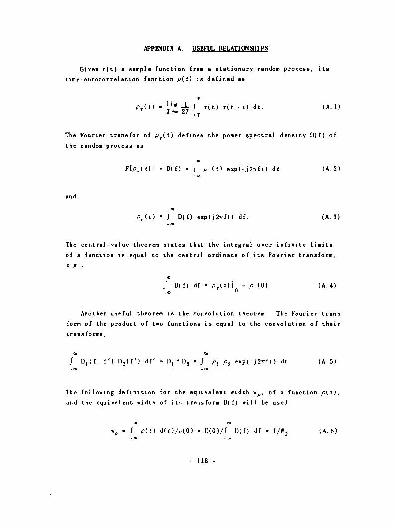
APPENDIX A. USEFUL RELATIONSHIPS

Given r(t) a sample function from a stationary random process, its

time-autocorrelation function p(;) is defined as

T

PrUt) - I'm 1 f r(t) r(t. t) dt. (A.1)I w 21 T

The Fourier transfor of Pr(t) defines the power spectral density D(f) of

the random process as

F[Pr(t)] - D(f) - f p (t) exp(-j2nft) dt (A.2)-Co

and

Pr(t) " f D(f) exp(j2vft) df (A.3)-0

The central-value theorem states that the integral over infinite limits

of a function is equal to the central ordinate of its Fourier transform,

e g,

f D(f) df - Pr(t) 0 - p (0). (A.4)

Another useful theorem is the convolution theorem. The Fourier trans.-

form of the product of two functions is equal to the convolution of their

transforms,

f Dl(f f') D2 (f') df' D1 D2 f P1 P2 exp(-j2vft) dt (A.5)

The following definition for the equivalent width wp, of a function p(t),

and the equivalent width of its transform D(f) will be used

O0 Co

wp f p(t) d(t)/p(O) - f(O)/f l)(f) df - l/WD (A.6)

- 118-

This relationship between the autocorrelation functions for the in-

put and output of a square-law detector has been given by Rice [Ref. 29]

Pout(t) - 2p~n (t) +p? n(0), (A.7)

from which we can write

B(f) - 2 fpin Pin exp(-j277ft) dt+P~n(O) 8(f) (A.8)O

where 6(f) is the unit impulse function.

119 -

APPENDIX B ANALYSIS OF A CORRELATION RECEIVER

The receiver analysed below is the one shown in Fig. 4.3, and the

assumptions used are as follows

1. All random voltages arise from stationary gaussian processes andhave zero mean values

2 All noise contributions of a receiver channel are lumped intoequivalent thermal sources at the channel input.

3 Calibration procedures result in a one degree increment of inputtemperature yielding a unit deflection increment at the output.

4. The smoothing filter bandwidtlh H(f) is much narrower than thereception filter bandwidth G(f).

At the multiplier, the two input voltages are

xl(t) - nl(t) + (s/V')(t) (vl/4)(t) + (v 2 /4)(t) (B 1)

and

x 2 (t) - n 2 (t) ' (sl/v2)(t) (v,/4)kt) - (v 2/4)(t) (B 2)

The butput of the multiplier

ykt) - x 1 x 2kt) *(n n n2s/V2 (n 2v 1 /4) (n 2 v 2 /4)

(njs/v/2j , ks2/2) (nlv,/4)- (nlv 2/4)

v/1 vv/ 2v/16) (B 3)

The power spectrum of the receiver output is related by the Fourier

transform to the autocorrelation function of y(t) which is

f (_) -: 'y(t) ykt +T) (B 4)

Only the non-zero terms are contained in the expansion below, where we

write

120 --

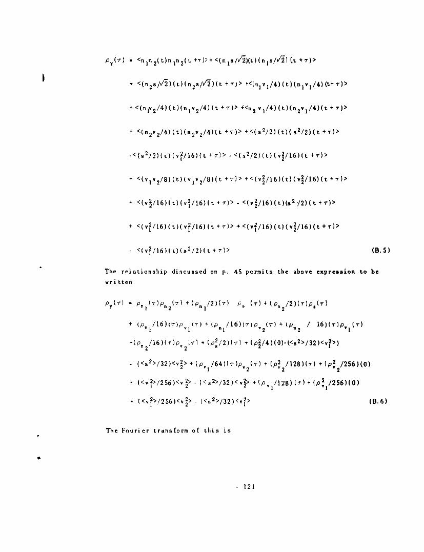
py) <nIn 2(t)nln 2(L +T),+<(nls/v/2)(t)(n s/2)(t + r)>

+ <(n2 s/v/)(t)(n 2 s/'2)(t +T)> <(nlv 1/4)(t)(nlv1 /4)(t+T)>

+ <(nIv 2 /4) ( t)(niv2/4) (t +r") > +<n 2 v 1/4) (t)(n 2v 1/4) (t + 7)>

+ <(n 2 v2/4) (t)(n2v2/4)(t +T)> +<(s 2/2) (t) (s2/2) (t +T) >

-< (s82/2) (c)(v2/ 16) (t + ) > - < (s2/2) () v2/16)(t + ) >

+ <(v v2/8)(t)(v v2/8)(t +T)> +<(v2/16)(t)(v2/16)(t r)>

+ <(v2/l6)(t)(v2/i6)(t +T)>- <(v2/16)(t)(s2 /2)(t +r)>

+ <(v2/16)(t)(v2/16)(t +)>+<(v2/16)(t)(v2/16)(t+ }>

- <(v2/16)(t)(s 2/2)(t+T)> (B. 5)

The relationship discussed on p. 45 permits the above expression to be

written

(-r) - p ('r)p (r) +(Pn /2)(T) ,; (.r) + (Pn2 /2)(r)p (r)

+ (p n/16)(r)PV (r) + (Pn /16)(r)p 2 (-r ) + (pn 2 / 16)(,r)p, (r)

+(p /16)(-,)pV -i + (p2/2)(,) + (p2/4)(O)-(<s 2 >/32)<v2>)n 2 221

(<s2>/32)<v2> + (p, /64)(T)p (T) + (p2 /128)(r) +(p2 /256)(0)21Y Y2v2

S(<v>/256)v (<s/32)<v> /128)(r)+ /256)()

+ (<v2>/256)<v2>- (<s2 >/32)<v2> (B.6)

The Fourier transform of this is

121

B(f) k2 GGWTr rj + (T/2)(Ter +T e ) +[TrTc + TTC)/16]

+TeT )/161 + (T2/2) + (TCTC /64) + [(T 2 +Tc 2 )/128])+ (Ter2TCl er2Tc2 )

C 2 1

+ k2 ID G(f)df] 2 ((T2/4) + (TcITC2/128) - (T/16)(Tc AT C 2)

+ [T2 +T2 )/25611 (B.7)C1 C2

At the receiver output the power spectral density is

C(f) - B(f) II(f) (B.8)

Using C(f) the mean meter deflection <y>, the signal power S and the

noise power N can be found. Thus

<y> - k~i(0)] f G(f) df [(T/2)- (TC /16)- (Tc2/16)] (B.9)- C

S - ki1(0)] f G(f) df AT/2 (B. 10)

and

N - k 11(f) df (G*GI 0 Tes (B.11)

With a unity signal to noise ratio

S/N = - 11(0)

G SG I [Of(df) if 2TeS{ 0 - h(

Sv2Af AT/Te5. (B. 12)

122 -

From which we get

A T '2 / V'A--) I... (B.13)

The system effective noise temperature

Tea a (TerjTer 2 + (T/2)(Ter, +I er2) +[(TerlTCI +TerT C2)/16]

+ [r 1 + I T )/16) + (T 2 /2) + (TC Tc /64)[e r 2"C1 1e r 2 2 1"(2

+ ((Tc 2 +Tc2)/128]15 (B.14)1 2

For identical channels, when

Ter, Ter 2 Ter

and

I • I C2

Equation (B.14) simplifies to

Te. a [T2 T+ ( e + (12/2) + (T2/32)] (B. 15)

so that wien I/Ter and T C/T er are less than I,

Te. 2 Terf 1 + (l/21.er)[T + (1.C!4)]}

. Ter + (T/2) + ('C/ 8 ) (B. 16)

Using this expression for es we find

AT 2 [, + (1/2) + (Tc/8)) (B. 17)

1.23

APPENDIX C. DETAILED ANALYSIS OF THE MODULATED BECEIVER

The modulated receiver is shown in block diagram form in Fig. 3.1.

This illustration includes all the components of the elemental receiver

plus additional components to perform the modulation and demodulation.

A function generator, a modulator, and a coherent demodulator are neces-

sary. The video-frequecy filter is not essential but is usually present

in practice.

The procedure followed will be to calculate the power spectral den-

sity at the output of the receiver and from this determine the signal-

to-noise ratio. The minimum-detectable input-temperature increment

produces a unity signal-to-noise ratio.

The equivalent source temperature for the reception-filter input will

be

Ter +T T(t)

where

T 7(t) - T7 (t) (T -Tref) +Tref

. [(T- Tref)/2][1 - p(t)] +Tref (C. 1)

The waveform p(t) determines the form of the power modulation.

At the detector output the voltage y(t) is a measure of the instantane-

ous power. When averaged over times long compared with w (an equivalent

width of tie autocorrelation function for y(t)], but short compared with

the modulation period, we describe this function approximately as a

varying time-average

<y>(t) 2 <x2 >(t) - k j G(f) df {Ter +Tref + [(T -Tref)/2 1 [1 -/u(t)]) (C.2)

If we form an expression for x(t) as tle sum of two voltages derived from

the modulated source and the effective receiver input noise temperature

Ter +1re, we have

x(t) = M(t) v(t) +n(t) (C.3)

- 124

and

<x2>(t) - <u 2 (t)> ?.'(t) +<n2(t)> (C.4)

where

<*()' k fG(f) df (Ter +Trf)

*n() k f GMf df (T-Trf) (C.5)

and

V2 (1 .dt)]/2 - 7)(t)

Since ji(t) is descriptive of the form of modulation, v(t) is seldom

speci fi ed.

First we consider the case for JMf - 1. Then

y2(t) =y(t) 9(t) -x 2(t) f(t). (C.6)

The autocorrelation function

(r) . rn I r x(t) x(t+7r) x(t) x(tI-r) g(t) f(t4-r) dt

* <x(t) x(t-r) x(t) x(t+r) (t) e(t4-r)>

* <an2 (t ) 7 t ) + 2a (t) n t ) v ( t +n 2 (t) ]

From this expression the following terms have non-zero values:

- 125 -

After evaluating the random portions of these expressions we have

[<m2(t)>2+2p2(.r)] <7)(t) 77(t4-r) 6(t) g(t+.r)>

4p,(7-) po(r ) <v( t) v( t+T) ( t) g(t+,r)>

2p2(7-) < (t) (t. rH> +<n2(t)> 2 < (t) f(t+7-)>

The periodic portion of the first term can be written

<{ 11 - P( t)/$l P- yt+T)] 0 (t (t+T)>

<1/4 [1 - A(t) -At( t r) +y( t) p(t+-r)] g( t) (t4-r)>

The only d-c component (which must be signal) is determined by the mean

value of the term

1/4 <P(t) u(t+T) (t) 4(t+r)>.<n2 (t)>2

Now, since we are interested in determining the signal-to-noise ratio at

zero signal, the noise-power spectrum is that which is the Fourier trans-

form of

2p2(-r) < '(t) %'.(t+T)>

The mean value or d-c component of an autocorrelation function for a

periodic function is equal to the square of the average value of the

function over a period T. Thus

S H(0) P t) (t) dt <M2(t) > 2

= H(0) -4 k (T-Tref . (f) df f0 /(t) 1(2 dt (C8)

When S( t ) is wri tt;n in I-ouri er .cri es lfnrm,

K(t) K4n exp(nj27Yfmt) exp(njo). (C.9)

- 126 -

Th en

OD 2<e(t) I(t+)> - . IK.n 2 exp(nj277far) (C. 10)

The noise-power spectrum at the output of the receiver is

CC(f) {2k 2(T er+Tref)2 [G G] * --2 IKe 12 6(f- nf) H(M) (C.11)n a -Go n

This spectrum is very wide compared with the spectrum of (t); therefore,

to a close approximation, we can write for the noise-power output

N = 2k2(Te r+T'rf)2 [G*GI ° Ken 1f It(f) df. (C.12)lb-0 - C

Now, making use of the definitions for r and Af we form the signal-to-

noise power ratio and set it equal to unity, thus

T 2 002H(O) f Li t g(t) dt k2AT Gf) df

N2 2 'D

N2 2k2(Tr +T~ )2 [G lKe I f~ If(f) df

T 12I AT T f J'U(t) d(t) dt

0 (C. 13)2

(Ter +Tref) 2 IKn

r - w l

From this we find the minimum detectable input temperature increment

6T (T +'ref) //VI/,rT (C.14)

where

127

I Ke, t 2M - 2 n--m 2 t2 C 5

(I/ ) f /(t) 6(t) dtj /) f ju(t) e(t) dtf)a0 0

Interest centers on minimum values for M, given explicit waveforms. The

phase of (t) must be set for the maximum value of the denominator in the

above expression in order to achieve the minimum M. Table 4.1 contains

values of M for various combinations of u(t) and S(t).

In order to include a video filter in the analysis we need the de-

tector output spectrum. Knowing this the effect of the video filter can

be considered and the spectrum at the input to the coherent demodulator

can be determined.

The autocorrelation function for the detector output is

pY(T) - <x(t) x(t+r) x(t) x(t+r)> (C.16)

The non-zero terms in this expression are

< 42(t)> 2 <71(t) 7)( t+ -r)> + 2P2 ( r) < 7i( t) 7)(t+ r) >

4pn, ) pn(,r) <Y(t) uv(t+,r)>

<n2(t)> 2 +2p2(r)

For zero signal conditions the noise power is derived from the term

2p2('r)

and the signal-power information is in the term

<M2( t)>2 .<?( t) 7)( t+.r)>.

The Fourier transforms of these terms times the power-transfer character-

istic of the video filter are the noise and signal components of the

power spectrum given below

- 128 -

B (f) - 2k2 (Ter +Trf) 2 G G J(f)e2

+ k2 (T - Tref) 2 G(f) df 2F[<r(t) 7)(t+-r)>] J(f). (C.17)

Two forms for J(f) of interest are,: (1) a response that excludes fre-

quencies in the band around twice the reception filter mid-frequency,

as is common for envelope detectors, and (2) a narrow band including only

the fundamental of the modulation frequency. For the first case, since

f. must be small compared to Af, all the harmonics of j(t) will pass andcontribute to the signal-power output. The noise power output will be

the same as with no filter and hence the factor M is no affected.

In the second case, let J(f) - 1 for all significant values of H(f - fo)

and |I(f + fM); i.e., the smoothing filter is much narrower than the pass

band of the filter J(f). Then, for the noise component of the output

spectrum we can write

2k2(Ter +Tref) 2 G*GI0 2 IK 12 H(f)

since only the fundamental component of the demodulating signal gives

rise to power within the smoothing-filter passband. The signal component

of the power spectral density at the output of J(f) is

(k2/4)(T- Tref) 2 G(f) df] F[<m(t) u(t+7)>] J(f)

or

-OD2('k2/4)(T -Tref)2 fG(f) df] [~K 2 5( f+f i) + I K, OA2(f f 0*)].

CO

when AA(ef) 2 K ,n exp(jn2ift). This can be associated with a voltageYl ( t

) , -Yhere n - -c

y1 (t) = (k/2)(Il Tref)I G(f) d] 21KMI cos 27rfrt (C. 18)

Now at the output of the coherent demodulator

- 129 -

Y2(t) • YI(t) (t)

and

P r) (T- Tref) 2 [:G(f) df 2 1K, 1 <cos 277fMt cos 27f (t+r) •

f(t) f(t+'r)>, (C. 19)

from which as in Eq. (C.8) we can write for the signal-power output

S 2 - II(O)k2(r'lref)2 [(f) d K 2 [1/7) f(t) cos 277fmt dt (C.20)-O 0

Determining the signal to-noise power ratio as before

AT2 rAf (1/T) f 7(t) cos 27lfmt dt IK 12

S2/N 2 1 0 (C. 21)

(Ter +Tref)2 2KfI 12

So we find

AT M (Ter +'ref) /1/76f

where

M V2 (C. 22)

IKI l/I) f "(t) cos 2irfmt dt0

For the case when the relative phase of ji(t) and '(t) is zero i.e.,

& - 0,

TIK I - (1/7) f (t) cos 27ifmt dt,

0

-130 -

since this just one-half times the expression for the fundamental

coefficient in a cosine Fourier series(Kel is the positive frequency

fundamental coefficient in the exponential form of the Fourier series).

This substitution results in the simplified expression

M 2- b2/IK A (C. 23)

In Table 4.2 values for M witb three different waveforms for U(t)

hai ! been calculated.

When a phase angle & exists between the fundamental components of I.(t)

and '(t),

T(1/7) f w(t) cos 2yfmt dt - JK'IJ cos a (C.24)

0

and

N' /2/IK i cos 6 (C. 25)

131 -

APPENDJIX D. PROOF OF THEOREM ON TIME IJISPLACEJIENTS DUE TO SMOOTHING

THEOREM: The centroid of the signal waveform t. will be located t

sec in time before the centroid of the recorded waveform tr, where th is

the time coordinate of the centroid of the impulse response in relation

to its origin or time of impulse.

GIVEN: A signal s(t), a smoothing filter with an impulse response

h(t), and the output signal r(t). We define the time coordinate of the

centroid of the waveform as t, which, for r(t), is expressed

f t r( t) dt

t r

J' r( t) dt- CD

TO PROVE:

t a r - h

PROOF: We use the relationships

Ca

BA'(O)/-j2-n - t r(t) dtQD

and

H(0) - r(t) dt

so that

11 R(0)/ j277 1(0)

and sini laril~y for the other functions, where 11(f), the Fourier transform

of r(t), can be written terms of the transforms of s(t) and h(t) as

H1(f) = S( f) 11( f).

.132

The derivative of this expression is

I'(f) - S(f) H'(f) +S'(f) M1(f).

Now we can write

S(O) 11(0) S(O) 11(0) -.

0 0'f 1f

S'(O)/-j27Y S(O)

t

Q.E.D.

The impulse response may have its centroid located at the origin when

it has a zero first moment and has a positive area. In this case the re-

corded waveform centroid will not be shifted relative to the signal wave-

form Lut serious distortion of shape will occur.

The tendancy exists for the evaluation of the centroid of a waveform

by eye to be made on the basis of the area under the absolute value of

the waveform. For applications such as those involving smoothing, this

must be avoided. In general, smoothing filters with oscillatory responses

which may have zero first moments are not used, but in servo type re-

ceivers ttie possibility exists.

- 133 -

APPENDIX E. DETAILS OF TE VARACTOR DIODE SHORTING SECTION

The varactor diode is mounted in the center of the broad face of the

guide, grounded to one wall and with a switching-signal connection fed

tbrough a by-passing mount to a BNC connector. \ ith the diode so mounted

and electrically connected to the switching voltage of reversable polarity,

a measurement of th-e minimum S.rR present was made for any position of the

short behind the diode. This minimum S1.11 is indicative of the losses

present and hence expected loss in the device when used as a variable

short. For the two states of tie diode the predominant change is in the

susceptance. A given susceptance change yields the greatest phase-length

change when the two values are equal but of opposite sign. This condition

for the susceptance can Le met since tbe adjustment of the short pusition

moves the admittances alcng nearly constant-G circles on the Smith chart.

When adjusted in tlhat manner, the maximum phase-length change observed

for the W1E 427A diodes was 88 percent of the required quarter-wave. A

full quarter-wave shift could ce obtained if these admittances were

transformed to unity per unit magnitude. A quarter-wave transformer section

made with a dielectric slaF accomplished this transformation and the re-

quired phaselength' change was observed. An alternative procedure that

is presently being used is to taper the waveguide so that the diode is

mounted in the proper guide admittance.

As well as having the quarter-wave shift, one of the sections must

have a total path length longer than the other by a quarter wave. Conse-

luently, one of the diode sections was made that much longer so that,

after separate adjustment of the quarter wave change had been made, the

complete assembly could he finally adjusted with shim-like sections of

waveguide and small polystyrene blocks in th.e guide.

- 134 -

REFERENCES

1. R. H. Dicke, "The Measurement of Thermal Radiation at MicrowaveFrequencies," Rev. Sct. Instr., 17, 7, pp. 268-275, July, 1946

2. A. E. Siegman, "Thermal Noise in Microwave Systems," Microwave J4, 3-5, pp., 81-90, 66-73, and 93-104, March, April and May, 1961.

3. "IRE Standards on Methods of Measuring Noise in Linear Two-Ports.1959", Proc. IRE, 48, 1, pp. 60-68, January 1960.

4. P. D. Strum, "Considerations in High-Sensitivity Microwave Radiometry,"Proc IRE, 46, pp. 43-53, January, 1958.

5. D. G. Lampard, "The Minimum Detectable Change in the Mean Noise-Input Power to a Radio Receiver," Proc. IEE, 101, Part IV, pp.118-128, February, 1954.

6. E. J. Kelly, D. H. Lyons, and W. L. Root, "The Theory of theRadiometer," MIT, Lincoln Lab. Group 312, Group Report 47.16,2 May 1958.

7. J. L Steinberg, "Receivers for Radio Frequency Noise. I. Measure-ment of Temperature by Means of Thermionics Radiation Using veryHigh Radio Frequencies," Onde elect. 32, pp. 445-54, November 1952.II. Gain Fluctuations in Measuring Apparatus. Use of Modulation,"Onde elect. 32, pp. 519-26, December 1952.

8. R. ,N. Bracewell, "Radio Astronomy Techniques," Handbuch der Physik,54, S. Fliugge, Ed., Springer, Berlin (in press)

9. W. Selove, "A d-c Comparison Radiometer," Rev. Sci. Instr., 25,I'' pp. 120-122, February, 1954.

10. S. J Goldstein, Jr., "A Comparison of Two Radiometer Circuits,"Proc. IRE, 43, pp. 1663-1666, November, 1955.

11. 1). G. Tucker, M. H. Graham, and S. J. Goldstein, Jr., "A Comparison

o! Two Radiometer Circuits," Proc. IRE, 45, pp. 365-366, March, 1957.

12. C. L Seeger, F. L II. M. Stumpers, and N. van lurck, "A 75 cmReceiver for Radio Astronomy and Some Observational Results,"Philips 7ech Rev., 18, pp. 141-144, 1956/1957.

13. R M. Sloanaker, J. II. Nichols, "Measurements of the Positions,Fluxes, and Sizes of Celestial Radio Sources at 10.2 cm," NRL ReportNo. 5485, U. S. Naval Research Laboratory, Washington, D. C., Jily13, 1960.

14. C. L. Seeger, "A Tentative Measure of tle Flux Density of CassiopeiaA at 400 Mc/s," I.A./., 13, 472, pp. 100.104, November 1956

15. R. Adgie and F. G. Smith, "The Radio Emission Spectra of FourDiscrete Sources and of the Background Radiation," Obs , 76,894, pp. 181..187, 1956.

16. N. W. Broten and W J. Medd, "Absolute Fluk Measurements ofCassiopeia A, Taurus A, and Cygnus A, at 3200 Mc/s, 4strophys Jour.

132, 2, September 19.60.

135 -

REFERENCES (Cont'd)

17. M. Ryle and D. D. Vonberg, "An Investigation of Radio-FrequencyRadiation from the Sun," Proc. Boy. Soc., A, 193, p,. 98-119, 1948.

18 D. Middleton, An Introduction To Statistical Communication Theory,McGraw-Hill Book Co., Inc., New York, p. 343, 1960.

19. E J. Blum, "Sensibilite des Radiotel6scopes and Recepteurs aCorrelation," Annales d'Astrophysique, 22, 2, pp. 140-163, March-April, 1959

20. L. D. Strom, "The Theoretical Sensitivity of the Dicke Radiometer,"Proc. IRE, 45, pp. 1291-1292, September, 1957.

21 B M. Oliver, "Automatic Volume Control as a Feedback Problem,"Proc. IRE, 36, pp. 466-473, April, 1948.

22. K. E. Machin, M. Ryle, and D D. Vonberg, "The Design of an Equipmentfor Measuring Small Radio-Frequency Noise Powers," Proc. IEE, pt. III,99, pp. 127-134, May, 1952.

23. J G. Truxal, Automatic Feedback Control System Synthesis, McGraw-Hill Book Co., Inc., New York, pp 80-87, 1955.

24 R. N. Bracewell and G. Swarup, "The Stanford Microwave Spectro-heliograph Antenna, a Microsteradian Pencil-Beam Antenna," IRE Trans.on Ant and Prop., AP-9, 1, pp. 22-30, January 1961.

25. G Swarup, "Studies of Solar Microwave Emission Using a HighlyDirectional Antenna," SR No. 13 [AF18(603)-53], AFSOR No. 265,Stanford Electronics Laboratories, Stanford University, Stanford,California, p. 31, February 6, 1961.

26 G. Swarup, "Stanford Microwave Spectroheliograms for 1960 April,May, and June;" Scientific Reports No. 8, 10, and 11. [AF18(603)-53],Stanford Electronics Laboratories, Stanford University, Stanford,California, December 15, 1960, January 15, 1961, and April 28, 1961.

27 V. I. Bunimovich, "Radiometer Sensitivity," Zhurnal 7ekhnicheskoiFiziki, 20, 8, pp. 944-953, 1950 (In Russian).

28. P ). Strum, "Correction to 'Considerations in High-SensitivityMicrowave Radiometry'," Proc. IRE, 47, 12, p. 2105, December 1959.

29. S. 0. Rice, "Mathematical Analysis of Random Noise; Part IV, NoiseThrough Non-Linear Devices," Bell System Tech. Jour. 24, pp. 115-156,1945 (In particular p. 149.)

- 136 -

DIoBMIM!0 LS? - AP8(603)-53

NoedwYr 1961

or Scientific Re Arnold Air Pores StationWahington 25, D.C. TWausI'e Tonneee

3 Attnt SRYP 1 Attn: AZbC LibrarY

Comander com rA? Research Division AP Flight Test Center2 Ahtt 1.C. Iduarns Air Force Base, Clif.Wamhng~_._25, D.C.Atn Y2Attni IMM Attnt VTOTL

Oommnder comanderWright Air Development Divisior Ait1 Spe i Feaocns e Ut. .

Wright-Patterson AI, Ohio Kirtla W e , spOl Ct .M.4 Attn: ASAPRD-DIST 1 Attni SWOr

Commnder ComnderAF Cambridge Res. Laboratories AP NisillS Dav't Ctr.

L.O. Hanscom Field Holeman APB# NeW MexicoBedford, asachunettS I Attnt RDOI

1 Attn, CRRAL CommanderCommander Army Rocket & Ouided Missile

Rome Air Development Center AgencyOriffils Air Force Base Redstone Arsenal, AlLRom, New York I Attnt ORDX'R-OTL

1 Attn: RCOYL-2 Ce MlWt

Comnder AP Institute of Tech.(AU Lib)

Detacheent 1 NCLI-LIB, Mdg., 125, Area B

g kF Research Division 1 Wright-ftterson APB, OhioThe Shell Building

2 Brussels, BDlOUU ComanderAir Research & Dev't Comnd

P.O. Box AA Andrew Air Force Base1 Wright-Patterson Air Porce fea. Washington 25, D.C.

Ohio 1 Attn M 2 eyeAttn: RDRA 1 cy

low Aeronautica Research Labs. RDRB I yWright-Patterson AI.S, Ohio MDRC 1 y

1 Attn: Tech Lib., Bldg. 45O RDRS 1 ay

8*' ASTIA Comnding GeneralArlington Hall Station U.S. Am Signal Corps R-.1.Arlington 12, Virginia an Davit Lab.

10 Attnt TIPCR Ft. Monmouth, New Jerey1 Attni SI0FNWL-RPO

Director of Res. and Dev'tHeadquarters, USAF National Aeronautics I SpaceWashington 25, D.C. Administration

1 Attn: ADRD 6 Washington 25, D.C.

Of fice of Naval Research Advanced Research Proji. A cyWashington 25, D.C. 1 Wahington 25, D.C.Department of the Navy

1 Attn: Code 420 Rand Corporation1700 Main Street

Director, Naval Res. Lab. 1 Santa Monica, CaliforniaWashington 25, D.C.

1 Attng Tech. in1fo. Officer ChalIrn, Canadian Joint Staff2450 MNasachusette Ave., N.W.

Director, Army Res. Oftice Washington 25, D.C.Dept. of the Ary 1 For DRB/bSIS

Washington 25, D.C.1 Attns Scientific Info. Dr.

Chief, Physics Br.Division of ResearchU.S. Atomic Energy Comission

1 Washington 25, D.C.

U.S. Atomic Energy ComansionTech. Info. ExtensionP.O. Box 62

1 Oak Ridge, Tennessee

National Bureau of StandardsLibray, fa. 203, KW Building

1 WVgnington 25, D.C.

tPhysics ProgramNational Science Foundation

1 Washington 25, D.C.

Director, Office of Ord. Res.Box CN, Duke Station

1 Durham, North Carolina

Director, Dept. of ComerCeOffice of Tech. Services

1 Washington 25, D.C.