UNCERTAINTY QUANTIFICATION AND ROBUSTOPTIMIZATION FOR THROUGHFLOW AXIAL COMPRESSOR

DESIGN

J. Sans - T. Verstraete - J.-F. Brouckaert

Turbomachinery and Propulsion Department, Von Karman Institute for Fluid Dynamics72, Chaussee de Waterloo, B-1640 Rhode-Saint-Genese Belgium,

sans@vki.ac.be

ABSTRACTThroughflow axial compressor design relies on empirical correlations to estimate the total pres-sure losses and deviation generated by a blade row. Those correlation data have been obtainedwith given measurement uncertainties that are usually not taken into account by meridional de-sign tools or throughflow solvers. Uncertainty quantification techniques such as Monte-Carlosampling or stochastic collocation can help to introduce uncertainties within those numericaltools and quantify their effects on the compressor performance at cheap computational costs.The throughflow solver used for this investigation is ACPreDesign. The code has been recentlyimplemented at VKI and solves the non-isentropic radial equilibrium equations for axial com-pressors. Realistic uncertainties are introduced from standard loss correlations. The imple-mentation of non-intrusive uncertainty quantification methods is presented and validated ona single stage low pressure compressor geometry studied at VKI. The results are analyzed interms of efficiency probability density functions which represent the resulting uncertainties onefficiency due to non-deterministic loss correlations. Finally, ACPreDesign is coupled to the VKIoptimizer CADO in order to approach the problem of design under uncertainty also referredto as robust design. To address that issue the paper focuses on a robust solidity optimization ofa single rotor configuration.

NOMENCLATURE

D Diffusion factor [-]Hn n-order Hermite’s polynomial [-]U uncertain input [ ]ζ Loss parameter [-]β2 Outlet flow angle [◦]η Efficiency [-]µ Average [ ]ξ Random variable [ ]σ Solidity [-]

or Standard deviation [ ]ω Total pressure loss [-]

CFD Computational Fluid DynamicsIGV Inlet Guide VaneNISRE Non-Isentropic Radial EquilibriumPDF Probability Density FunctionUQ Uncertainty QuantificationVKI von Karman Institute for Fluid Dynamics

1

Proceedings of

11th European Conference on Turbomachinery Fluid dynamics & Thermodynamics

ETC11, March 23-27, 2015, Madrid, Spain

OPEN ACCESS

Downloaded from www.euroturbo.eu Copyright © by the Authors

INTRODUCTIONThe meridional design is an essential step in the elaboration of any turbomachinery component.

Many choices, such as the channel geometry or the solidity, are done at the level of the meridionaldesign and may influence the rest of the whole design process.

However, any radial equilibrium solver relies on empirical correlations. Those correlations pro-vide an estimate of the total pressure losses of a blade row depending on its loading and number ofblades. For compressors, such correlations originally come from the work of Lieblein et al. (1953)but have been completed to provide spanwise corrections like in the work of Robbins et al. (1965).Nevertheless, it must not be forgotten that all empirical correlation data have been obtained withingiven measurement uncertainty bands. Similarly, many correlations often present a big scatter in thedata due to the wide variety of tested profiles and a polynomial curve fit is usually drawn through themeasurement points to allow for an implementation in a throughflow solver. The uncertainties or thedata scatter is then neglected.

Since nowadays meridional calculations are very cheap in terms of computational time, it is veryappealing to combine throughflow solvers with optimizer tools and/or with uncertainty quantification(UQ) techniques which both require many evaluations such as evolutionary algorithms or Monte-Carlo sampling and stochastic collocation techniques.

The main purpose of UQ methods is to improve the confidence in any numerical prediction byconsidering a probabilistic framework and epistemic uncertainties. These are defined as a potentialdefect or deficiency due to a lack of knowledge. They may be seen as model uncertainties. As anexample, the geometrical variability with respect to the theoretical design that may appear during themanufacturing or because of some damages occurring during the engine life cycle may be seen asa source of epistemic uncertainties. Those are usually disregarded, especially at the early phase ofthe meridional design. Nonetheless, the impact of those geometrical variabilities at the level of thethroughflow design have been studied by Lecerf et al. (2003) or Panizza et al. (2014) respectivelyfor high-pressure compressors and centrifugal compressors. In any CFD computations, the turbu-lence models are another important source of epistemic uncertainties that are not taken into accountby deterministic approaches. Similarly, the uncertainties related to any loss or deviation empiricalcorrelations in a meridional solver are most of the time neglected and the originality of the currentinvestigation resides in the consideration of the epistemic uncertainties of such empirical models bythe means of UQ methods.

The use of UQ techniques and how they are implemented into a design process is the main focusof the current paper. To illustrate the methods, the emphasis is set on the solidity optimization ofa given compressor geometry. After briefly presenting the compressor geometry and the solver, theresults of solidity optimization without UQ are firstly given. Based on those optimum designs, UQ isintroduced by using both sampling or quadrature methods. The loss correlations are parametrized toanalyze their impact on the results. The last issue addressed in the paper is the problem of optimizationunder uncertainty commonly referred to as robust design. The results are discussed with and withoutthe use of UQ.

AXIAL COMPRESSOR PRE-DESIGN TOOLThe meridional solver that is used is ACPreDesign. This multi-stage axial compressor design

program originally comes from Creveling and Carmody (1968) and has been recently implementedat VKI. It solves the non-isentropic radial equilibrium equations for given design input parameters.Currently, the program does not provide off-design predictions. Examples of meridional optimizationusing ACPreDesign can be found in the work of Joly et al. (2012) or Teichel et al. (2013).

2

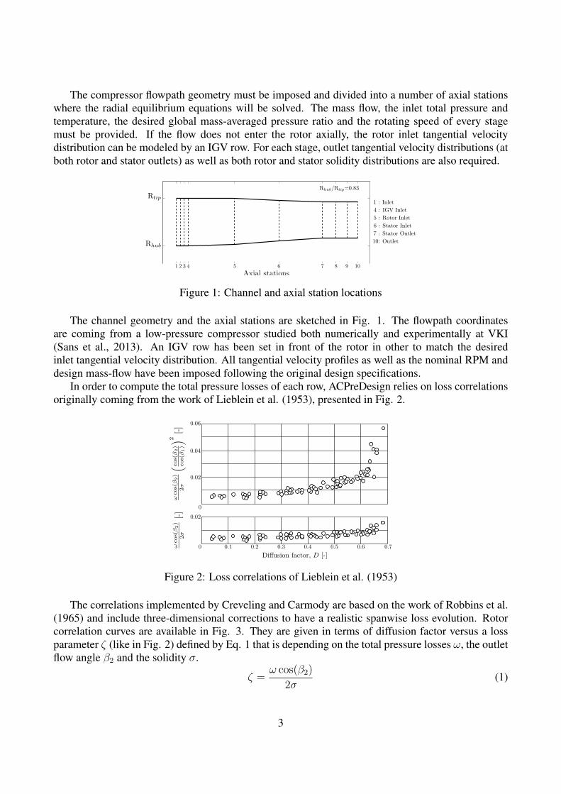
The compressor flowpath geometry must be imposed and divided into a number of axial stationswhere the radial equilibrium equations will be solved. The mass flow, the inlet total pressure andtemperature, the desired global mass-averaged pressure ratio and the rotating speed of every stagemust be provided. If the flow does not enter the rotor axially, the rotor inlet tangential velocitydistribution can be modeled by an IGV row. For each stage, outlet tangential velocity distributions (atboth rotor and stator outlets) as well as both rotor and stator solidity distributions are also required.

Figure 1: Channel and axial station locations

The channel geometry and the axial stations are sketched in Fig. 1. The flowpath coordinatesare coming from a low-pressure compressor studied both numerically and experimentally at VKI(Sans et al., 2013). An IGV row has been set in front of the rotor in other to match the desiredinlet tangential velocity distribution. All tangential velocity profiles as well as the nominal RPM anddesign mass-flow have been imposed following the original design specifications.

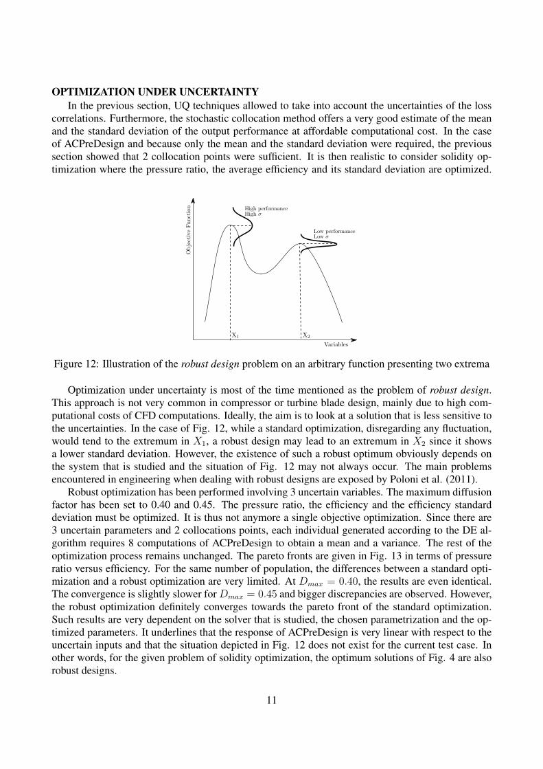
In order to compute the total pressure losses of each row, ACPreDesign relies on loss correlationsoriginally coming from the work of Lieblein et al. (1953), presented in Fig. 2.

Figure 2: Loss correlations of Lieblein et al. (1953)

The correlations implemented by Creveling and Carmody are based on the work of Robbins et al.(1965) and include three-dimensional corrections to have a realistic spanwise loss evolution. Rotorcorrelation curves are available in Fig. 3. They are given in terms of diffusion factor versus a lossparameter ζ (like in Fig. 2) defined by Eq. 1 that is depending on the total pressure losses ω, the outletflow angle β2 and the solidity σ.

ζ =ω cos(β2)

2σ(1)

3

The mid-span rotor loss evolution is the lowest as it only contains profile losses. The hub curve isshifted to a higher loss level to account for secondary flows and potentially corner vortex separation.The tip losses are equal to the mid-span losses until a diffusion factor of 0.40 which triggers thegrowth of losses due to the tip gap vortex.

0 0.1 0.2 0.3 0.4 0.5 0.60

0.01

0.02

0.03

0.04

D [-]

ζ[-]

HubMid-spanTip

Figure 3: Rotor loss correlations of ACPreDesign

From the comparison of Fig. 2 and Fig. 3, it clearly emerges that the scatter of Fig. 2 has notbeen implemented in the correlations of ACPreDesign. This is a typical example of an epistemicuncertainty.

OPTIMIZATIONMethod and constraintsACPreDesign has been coupled to the VKI optimizer CADO (Verstraete, 2010) to find the best

solidity distributions in terms of efficiency for a given pressure ratio distribution. The solidity is im-posed at three span locations (10%, 50% and 90%) and a 2nd order Bezier interpolation is used tocompute the solidity distribution. More that simply the global average pressure ratio, the whole pres-sure ratio spanwise distribution may be imposed. It is controlled through the rotor outlet tangentialvelocity distribution which is optimized together with the solidity distribution to satisfy the designrequirements both in terms of spanwise pressure ratio distribution and global average pressure ratio.

The VKI optimization code CADO is based on a differential evolution (DE) algorithm. This evo-lutionary method has been developed by Price and Storn (1997). Originally implemented for axialturbomachinery blade optimization, CADO has since then been improved and extended to multidis-ciplinary optimizations by Verstraete (2008). The algorithm can easily be coupled to any solver asin the present case to ACPreDesign. As mentioned earlier, the previous work of Joly et al. (2012)or Teichel et al. (2013) are very good examples of ACPreDesign optimizations using CADO. Themajor drawback of DE is that it requires a large number of evaluations which, in some situations, maybecome unrealistic depending on the complexity of the optimization problem and the solver. The useof metamodels may help to reduce the total computational cost but, in the case of ACPreDesign, thenumber of evaluations does not represent an issue.

Various constraints may be imposed by the designer. They may be set on aerodynamic perfor-mance parameters (maximum turning of the airfoil, diffusion factor etc...) or involve mechanicalconsiderations (maximum RPM). In the current situation, the most limiting parameter is the max-imum diffusion factor which has been constrained over the whole span. This parameter has a biginfluence on the results of the optimization. A constraint has been set on the pressure ratio at an arbi-trary level of 1.25. The problem becomes a single-objective optimization since only the efficiency ismaximized. The solidity is directly linked to the spanwise distribution of the chord length which maybe subjected to various mechanical additional constraints. Consequently, the solidity profile is not

4

completely arbitrary. Although no chord length limitation has been considered in the current paper,it must be mentioned that it is also possible to add specific constraints on the solidity or the chord aswell as on their slope or curvature. This can fasten the whole design process by taking into accountsome mechanical requirements of the latest design phase at the early stage of the throughflow design.

Optimum solidity distributionsThe constraint on the diffusion factor has quickly been identified as a crucial parameter. Opti-

mizations have been run varying the maximum rotor diffusion factor Dmax from 0.375 to 0.45 bysteps of 0.025 as well as for Dmax = 0.50. Optimizations have also been run on the full stage butonly the single rotor configuration results are presented in the paper.

The rotor optimum solidity distributions are displayed in Fig. 4 next to the corresponding diffusionfactor distributions in Fig. 5. Increasing Dmax, the mean solidity decreases. The trend of solidityversus span becomes linear for Dmax = 0.425 and then changes curvature for higher diffusion. ForDmax > 0.425, the tip solidity remains around 0.9. Looking at the corresponding diffusion factors, itseems that, for Dmax ≤ 0.425, the diffusion factor is higher at the hub than at the tip. More precisely,the diffusion level remains around 0.40 in the tip section. It underlines that an optimum diffusion liesaround 0.40 at the tip but does not remain optimal towards the hub sections.

0.5 1 1.5 20

20

40

60

80

100

Rotor Solidity [-]

Span[%

]

Dmax = 0.375Dmax = 0.40Dmax = 0.425Dmax = 0.45Dmax = 0.50

Dmax ↑

Figure 4: Optimum rotor solidity distributions fordifferent values of Dmax

0.3 0.4 0.5 0.60

20

40

60

80

100

Rotor Diffusion Factor [-]

Span[%

]

Dmax = 0.375Dmax = 0.40Dmax = 0.425Dmax = 0.45Dmax = 0.50

Dmax ↑

Figure 5: Rotor diffusion factor distributions fordifferent values of Dmax

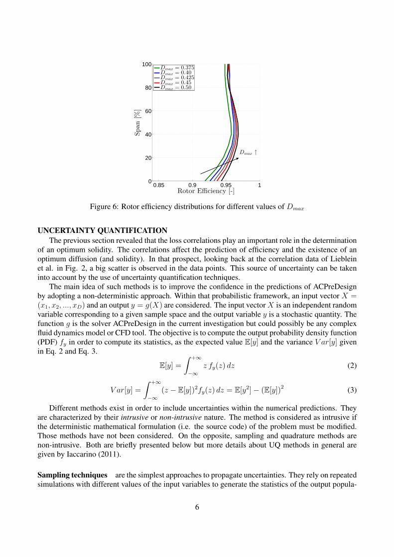
The rotor efficiency distributions in Fig. 6 show that higher efficiency is obtained with increasingDmax. While the hub and mid-span efficiencies always increase for higher Dmax, at the tip, theefficiency remains constant for Dmax > 0.40. It can also be noticed that for each value of Dmax,the highest efficiency is achieved at mid-span since the correlation curves of Fig. 3 always give thelowest amount of losses at mid-span. The highest efficiency is achieved with Dmax = 0.50 which isobviously a very theoretical result since a rotor enduring a diffusion factor of 0.50 at design wouldmost probably have no stall margin. However, as mentioned earlier, off-design predictions are not yetavailable in ACPreDesign.

5

0.85 0.9 0.95 10

20

40

60

80

100

Rotor Efficiency [-]

Span[%

]

Dmax = 0.375Dmax = 0.40Dmax = 0.425Dmax = 0.45Dmax = 0.50

Dmax ↑

Figure 6: Rotor efficiency distributions for different values of Dmax

UNCERTAINTY QUANTIFICATIONThe previous section revealed that the loss correlations play an important role in the determination

of an optimum solidity. The correlations affect the prediction of efficiency and the existence of anoptimum diffusion (and solidity). In that prospect, looking back at the correlation data of Liebleinet al. in Fig. 2, a big scatter is observed in the data points. This source of uncertainty can be takeninto account by the use of uncertainty quantification techniques.

The main idea of such methods is to improve the confidence in the predictions of ACPreDesignby adopting a non-deterministic approach. Within that probabilistic framework, an input vector X =(x1, x2, ..., xD) and an output y = g(X) are considered. The input vectorX is an independent randomvariable corresponding to a given sample space and the output variable y is a stochastic quantity. Thefunction g is the solver ACPreDesign in the current investigation but could possibly be any complexfluid dynamics model or CFD tool. The objective is to compute the output probability density function(PDF) fy in order to compute its statistics, as the expected value E[y] and the variance V ar[y] givenin Eq. 2 and Eq. 3.

E[y] =∫ +∞

−∞z fy(z) dz (2)

V ar[y] =

∫ +∞

−∞(z − E[y])2fy(z) dz = E[y2]− (E[y])2 (3)

Different methods exist in order to include uncertainties within the numerical predictions. Theyare characterized by their intrusive or non-intrusive nature. The method is considered as intrusive ifthe deterministic mathematical formulation (i.e. the source code) of the problem must be modified.Those methods have not been considered. On the opposite, sampling and quadrature methods arenon-intrusive. Both are briefly presented below but more details about UQ methods in general aregiven by Iaccarino (2011).

Sampling techniques are the simplest approaches to propagate uncertainties. They rely on repeatedsimulations with different values of the input variables to generate the statistics of the output popula-

6

tion. The most famous sampling approach is the Monte-Carlo method. As mentioned by Iaccarino,the strength of sampling resides in the fact that it is universally applicable and will always convergeto the exact stochastic solution if the number of samples tends to the infinity. The main drawback ofMonte-Carlo sampling is that the convergence is very slow as, to build the statistics, it requires a largenumber of realizations.

Stochastic collocation refers to quadrature methods used to compute the statistics of random vari-ables. Such methods enables to calculate the integrals (such as Eq. 2 and Eq. 3) from a discrete(preferably low) number of realizations. The Gauss-Hermite quadrature is often used in the field ofuncertainty quantification. For random variables described by normal distribution, the formulation ofthe n-points quadrature is: ∫ +∞

−∞y(ξ) e−ξ

2

dξ ≈n∑i=0

wiy(ξi) (4)

where ξi are the roots of the Hermite polynomials Hn(x) and wi are weights to which the Hermitepolynomials are also associated. The weight wi is defined as,

wi =2n−1n!

√π

n2 [Hn−1(ξi)]. (5)

HavingH0(x) = 1 andH1(x) = 2x, Hermite polynomials are linked through the following recurrencerelation:

Hn+1 = 2xHn(x)− 2nHn−1(x). (6)

ParametrizationThe rotor loss have been parametrized with three uncertain parameters. The first parameter Umean

shifts the mean loss level of hub, mid-span and tip correlation curves. For a given value of diffusionfactor D, the rotor loss parameter is an independent normally distributed random variable of meanµ and variance σ. The mean µ is given by the default evolution of ACPreDesign of the rotor lossparameter versus diffusion factor, i.e. µ = ζ(D). The variance of Umean is constant over the wholespan and diffusion range and comes from the analysis of Fig. 2. Assuming that the data observed inFig. 2 corresponds to 95% of the individuals, it can be stated that the scatter is equal to 2 ∗ 1.96 ∗ σ =3.92σ. Finally, observing that the scatter is about 0.005 at constant diffusion, the variance σ is equalto 1.275 10−3. This parameter simply shifts the loss curves to higher or lower levels. For the hub andmid-span loss curves, Umean is the only uncertainty and both curves are just translated.

For the tip correlation curve, another parameter, noted UD, controls the value of the diffusionfactor where the losses start to rise. The last parameter Ustall introduces additional uncertainty on thelosses at stall, i.e. at D = 0.6. By changing Ustall independently from Umean and UD, the slope ofthe tip loss curve between the diffusion factor given by UD and D = 0.6 is varying. The situation isillustrated in Fig. 7 showing the three uncertain parameters Umean, UD and Ustall.

The choice of the mean and variance of UD and Ustall is more arbitrary. The variance of Ustall hasbeen set to two times the variance of Umean (i.e., σUstall

= 2 ∗ 1.275 10−3). For UD, a mean diffusionfactor of 0.4 and a variance of 0.01 have been considered. Those values are summarized in Table 1.

7

0 0.1 0.2 0.3 0.4 0.5 0.60

0.01

0.02

0.03

0.04

D [-]

ζ[-]

HubMid-spanTip

Umean

UD

Ustall

Umean

Figure 7: Rotor loss parametrization with three uncertain variables Umean, UD and Ustall

µ [-] σ [-]

Umean ζR(D) 1.275 10−3UD 0.40 0.01Ustall ζR(D = 0.6) 2.55 10−3

Table 1: Mean and variance of the three uncertain parameters Umean, UD and Ustall

ResultsConsidering the optimum solidity distribution of the previous section at Dmax = 0.45, Umean,

UD and Ustall have been randomly sampled 35.000 times although a minimum of 10.000 samplesis usually sufficient. After 35.000 computations of ACPreDesign, the statistics of this populationhave been analyzed in terms of pressure ratio and efficiency. Both Fig. 8 and Fig. 9 illustrate theconvergence of the efficiency mean and standard deviation. The minimum amount of samples isvery case sensitive and depends on the order of statistics that is required. In the current case, 20.000appeared sufficient since both the mean and the standard deviation do not significantly change above20.000 samples.

0 0.5 1 1.5 2 2.5 3 3.5x 10

4

95.94

95.95

95.96

95.97

95.98

95.99

96

96.01

Number of Samples

Efficien

cymean[%

]

Figure 8: Evolution of the efficiency mean withthe number of samples (Dmax = 0.45)

0 0.5 1 1.5 2 2.5 3 3.5x 10

4

0.34

0.35

0.36

0.37

0.38

0.39

Number of Samples

Efficiency

standard

deviation[%

]

Figure 9: Evolution of the efficiency standarddeviation with the number of samples (Dmax =0.45)

8

Before stochastic collocations may be applied, the user must know the nature of the output PDF.Indeed, depending on the kind of output PDF, different quadrature methods exist. Although Monte-Carlo sampling is very time and resource consuming, it remains the only way to characterize almostcontinuously the output PDF. To ensure a PDF is following a normal distribution, the population ispresented in a histogram as well as in a probability plot. To build such a plot, based on the resultingmean µ and standard deviation σ, a theoretical normal distribution N(µ, σ) is plotted against theobtained population that has been formerly sorted in ascending order. If the population is normallydistributed, the plot must look as a straight line. The histogram and the probability plot are shownin Fig. 10 which clearly proves the efficiency is normally distributed. The histogram in Fig. 10 alsogives a very good image of the scatter induced by non-deterministic loss correlations on the efficiency.Depending on the required confidence interval, the width approaches 1.5%.

94 95 96 97 980

200

400

600

800

1000

1200

Efficiency [%]

Nbr.

ofoccurren

ces[-]

Histogram

94.5 95 95.5 96 96.5 97 97.5

94.5

95

95.5

96

96.5

97

97.5

Theoretical Efficiency Cumulative Distribution [%]

Efficien

cyCumulativeDistribution[%

]

Probability Plot

95%ConfidenceInterval

Figure 10: Efficiency histogram and probability plot (Dmax = 0.45)

Given that the output PDF is Gaussian, the Hermite’s quadrature may be used to perform stochas-tic collocation. Quadratures using 2, 3 and 4 points have been applied. Since there are three uncertainparameters, ACPreDesign must be run 8, 27 or 81 times in order to generate the output statistics. Re-sults of stochastic collocations are compared to Monte-Carlo sampling in Fig. 11 for both efficiencymean and standard deviation. It appears both efficiency mean and standard deviation are not changingsignificantly with the number of collocation points. It depends on the system that is studied and theorder of the statistics that is required. In the present case, it appears that 2 collocation points aresufficient to calculate the mean and standard deviation. Small differences are observed between theresults of the Monte-Carlo sampling and the stochastic collocation method but this is not surprisingsince neither the Monte-Carlo nor the collocation technique is perfect. The first would require aninfinite number of samples and the second is based on an approximation of an integral quantity. Asthe difference sits around 10−3%, it can be considered as negligible.

9

0 1 2 3 4

95.94

95.96

95.98

96

96.02

Nbr. of collocation points

Efficien

cymean[%

]

Monte-CarloStochastic Collocation

0 1 2 3 4

0.365

0.37

0.375

0.38

Nbr. of collocation points

Efficien

cystandard

deviation[%

]

Monte-CarloStochastic Collocation

Figure 11: Efficiency mean and standard deviation in function of the number of collocation points(Dmax = 0.45)

The same procedure has been applied to the optimum candidate at Dmax = 0.40. Results aresummarized in Table 2 for both optima at Dmax = 0.40 and Dmax = 0.45 using both Monte-Carlosampling and stochastic collocation. The mean, the standard deviation and the 95% confidence in-terval [µ ± 1.96σ] are indicated. The analysis of Table 2 reveals the importance of accurate andtrustworthy correlations. The minimum standard deviation of the stage efficiency reaches 0.37%.Nowadays, compressor designers seek for 0.1% efficiency increase using three-dimensional blade de-sign. Moreover, as seen in Fig. 10, it represents a 95% confidence interval that covers close to 1.5%.This study demonstrates that the meridional design may already bring a non-negligible amount ofuncertainty due to the correlations.

MONTE-CARLO SAMPLING

µ σ [µ ± 1.96σ]

Dmax = 0.40π [-] 1.2509 0.0012 [1.2509 ± 0.0024]η [%] 95.56 0.44 [95.56 ± 0.86]

Dmax = 0.45π [-] 1.2509 0.0011 [1.2509 ± 0.0022]η [%] 95.98 0.37 [95.98 ± 0.73]

STOCHASTIC COLLOCATION

µ σ [µ ± 1.96σ]

Dmax = 0.40π [-] 1.2509 0.0012 [1.2509 ± 0.0024]η [%] 95.55 0.43 [95.55 ± 0.84]

Dmax = 0.45π [-] 1.2509 0.0011 [1.2509 ± 0.0022]η [%] 95.98 0.37 [95.98 ± 0.73]

Table 2: Monte-Carlo and stochastic collocations results using three uncertain parameters

10

OPTIMIZATION UNDER UNCERTAINTYIn the previous section, UQ techniques allowed to take into account the uncertainties of the loss

correlations. Furthermore, the stochastic collocation method offers a very good estimate of the meanand the standard deviation of the output performance at affordable computational cost. In the caseof ACPreDesign and because only the mean and the standard deviation were required, the previoussection showed that 2 collocation points were sufficient. It is then realistic to consider solidity op-timization where the pressure ratio, the average efficiency and its standard deviation are optimized.

Figure 12: Illustration of the robust design problem on an arbitrary function presenting two extrema

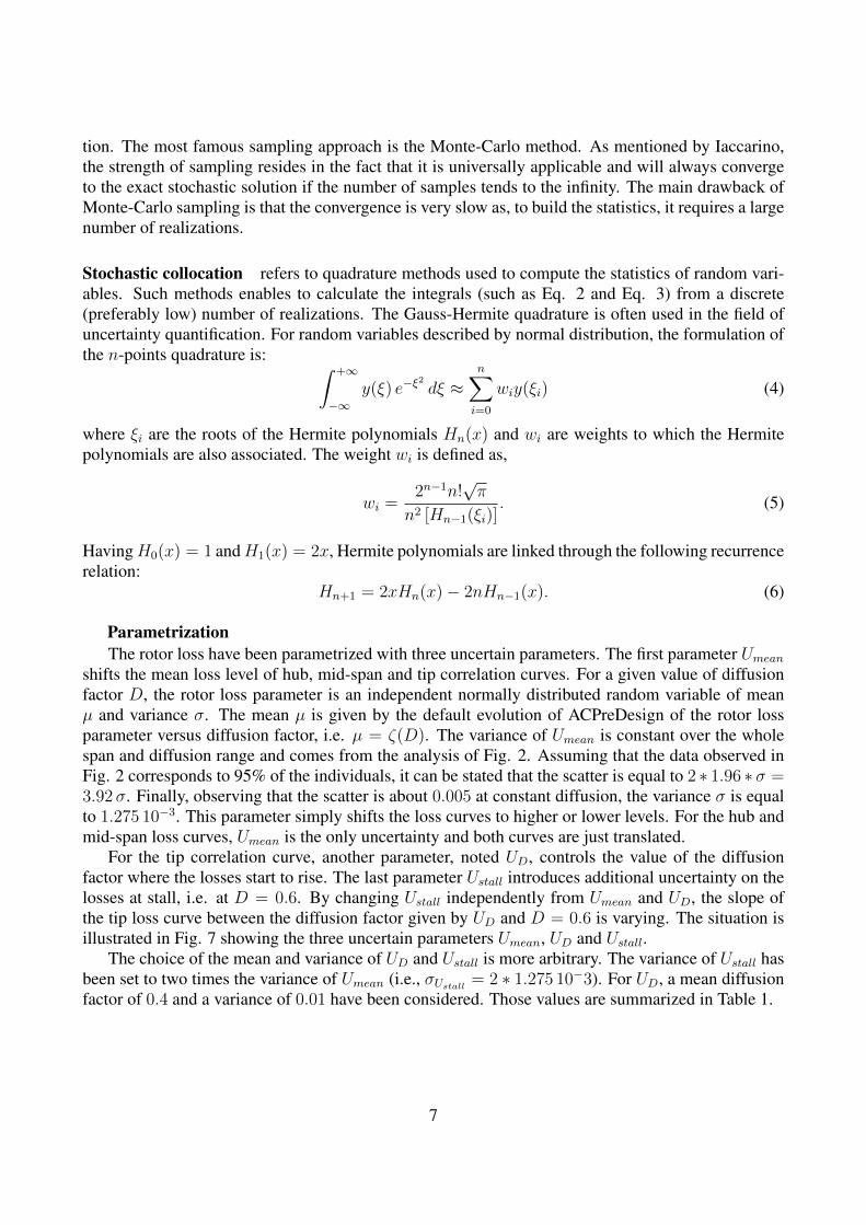
Optimization under uncertainty is most of the time mentioned as the problem of robust design.This approach is not very common in compressor or turbine blade design, mainly due to high com-putational costs of CFD computations. Ideally, the aim is to look at a solution that is less sensitive tothe uncertainties. In the case of Fig. 12, while a standard optimization, disregarding any fluctuation,would tend to the extremum in X1, a robust design may lead to an extremum in X2 since it showsa lower standard deviation. However, the existence of such a robust optimum obviously depends onthe system that is studied and the situation of Fig. 12 may not always occur. The main problemsencountered in engineering when dealing with robust designs are exposed by Poloni et al. (2011).

Robust optimization has been performed involving 3 uncertain variables. The maximum diffusionfactor has been set to 0.40 and 0.45. The pressure ratio, the efficiency and the efficiency standarddeviation must be optimized. It is thus not anymore a single objective optimization. Since there are3 uncertain parameters and 2 collocations points, each individual generated according to the DE al-gorithm requires 8 computations of ACPreDesign to obtain a mean and a variance. The rest of theoptimization process remains unchanged. The pareto fronts are given in Fig. 13 in terms of pressureratio versus efficiency. For the same number of population, the differences between a standard opti-mization and a robust optimization are very limited. At Dmax = 0.40, the results are even identical.The convergence is slightly slower forDmax = 0.45 and bigger discrepancies are observed. However,the robust optimization definitely converges towards the pareto front of the standard optimization.Such results are very dependent on the solver that is studied, the chosen parametrization and the op-timized parameters. It underlines that the response of ACPreDesign is very linear with respect to theuncertain inputs and that the situation depicted in Fig. 12 does not exist for the current test case. Inother words, for the given problem of solidity optimization, the optimum solutions of Fig. 4 are alsorobust designs.

11

93 94 95 96 97 98

1.15

1.2

1.25

1.3

1.35

Rotor Efficiency Mean [%]

RotorPressure

RatioMean[-]

Dmax = 0.40Dmax = 0.45Dmax = 0.40 - Robust DesignDmax = 0.45 - Robust Design

Dmax=0.40

Dmax=0.45

Figure 13: Comparison of pareto fronts with or without considering uncertainties

CONCLUSIONA meridional solver relies on empirical correlations to obtain an estimate of the total pressure

losses of a blade row. In the present investigation, the NISRE solver ACPreDesign is based on typ-ical correlations originally established by Lieblein et al. However, empirical data often come withuncertainties that are usually neglected at the level of the meridional design.

This paper investigates the use of uncertainty quantification methods in the specific case of solidityoptimization of a single rotor compressor. The study shows that both Monte-Carlo sampling as wellas quadrature method compute uncertainty bands that cover 1.5% in efficiency. While, nowadays,3D blade design optimization chases 0.1% improvements that are usually very difficult or impossibleto validate experimentally, it represents a non-negligible amount of uncertainty that are disregardedby a standard deterministic approach. Such additional information may imply to increase the targetefficiency according to the uncertainty band to guarantee a minimum efficiency above the designrequirements.

Outside the framework of solidity optimizations, uncertainty quantification could be implementedat the level of meridional design to take into account various sources of epistemic uncertainties. Forexample, the use of UQ techniques may compensate the lack of knowledge related to the influence ofthe inlet boundary layer profile, the Reynolds number or the inlet turbulence intensity which can causebig variation in the meridional design performance in terms of pressure ratio, efficiency and mass-flow. Off-design correlations also represents a tremendous source of uncertainty that can radicallyaffect the whole design. Finally, beyond the meridional design, non-deterministic CFD calculationsmay also play a crucial role in the management of turbulence modeling uncertainties.

The issue of the robust design was also addressed and, in the present case, the standard optimumdesign were already robust. The existence of a robust optimum strongly depends on the nature of theproblem that is studied and, in many situations, an optimization under uncertainty may lead to thesame solution as a standard optimization. Nevertheless, the study reveals the capability of performingmeridional robust optimization which may represent a breakthrough in turbomachinery design.

12

REFERENCESH. F. Creveling and R. H. Carmody. Axial Flow Compressor Design Computer Programs Incorporat-

ing Full Radial Equilibrium - Part I: Flow Path and Radial Equilibrium of Energy Specified - PartII: Radial Distribution of Total Pressure and Flow Path or Axial Velocity Ratio Specified. Technicalreport, NASA, June 1968. NASA CR-54531 and NASA CR-54532.

G. Iaccarino. Introduction to uncertainty representation and propagation. In Uncertainty quantifica-tion in computational fluid dynamics, RTO-AVT-VKI Lecture Series 2011/12 - AVT 193, Rhode-Saint-Genese, Belgium, October 2011.

M. Joly, T. Verstraete, and G. Paniagua. Full Design of Highly Loaded Fan by Multi-ObjectiveOptimization of Throughflow and High-Fidelity Aero-Mechanical Performance. In Proceedings ofASME Turbo Expo 2012, Copenhagen, Denmark, 2012. ASME Paper No. GT2012-69686.

N. Lecerf, D. Jeannel, and A. Laude. A Robust Design Methodology for High-Pressure CompressorThroughflow Optimization. In Proceedings of ASME Turbo Expo 2003, Atlanta, Georgia, USA,2003. ASME Paper No. GT2003-38264.

S. Lieblein, F. C. Schwenk, and R. L. Broderick. Diffusion Factor for Estimating Losses and LimitingBlade Loadings in Axial-Flow Compressor Blade Elements. NACA Research Memorandum, LewisFlight Propulsion Laboratory, Cleveland, Ohio, 1953. RME53D01.

A. Panizza, D. T. Rubino, and L. Tapinassi. Efficient Uncertainty Quantification of Centrifugal Com-pressor Performance Using Polynomial Chaos. In Proceedings of ASME Turbo Expo 2014, Dus-seldorf, Germany, 2014. ASME Paper No. GT2014-25081.

C. Poloni, V. Pediroda, and L. Parussini. Optimization under uncertainty. In Uncertainty quantifica-tion in computational fluid dynamics, RTO-AVT-VKI Lecture Series 2011/12 - AVT 193, Rhode-Saint-Genese, Belgium, October 2011.

K. Price and N. Storn. Differential Evolution. Dr. Dobb’s Journal, pages 18–24, April 1997.

W. H. Robbins, R. J. Jackson, and S. Lieblein. Aerodynamic design of axial-flow compressors -Chapter VII: Blade-element flow in annular cascades. NASA SP-36, 1965.

J. Sans, J. Desset, G. Dell’Era, and J.-F. Brouckaert. Performance Testing of a Low-Pressure Com-pressor. In The 10th European Turbomachinery Conference, Finland, 2013.

S. Teichel, T. Verstraete, and J. Seume. Optimized Preliminary Design of Compact Axial CompressorsA Comparison of Two Design Tools. In 31st AIAA Applied Aerodynamics Conference, San Diego,California, USA, 2013. AIAA-2013-2651.

T. Verstraete. Multidisciplinary Turbomachinery Component Optimization Considering Performance,Stress and Internal Heat Transfer. PhD Thesis, von Karman Institute for Fluid Dynamics - Univer-siteit Gent, Rhodes-Saint-Genese, Belgium, 2008.

T. Verstraete. CADO: a Computer Aided Design and Optimization Tool for Turbomachinery Appli-cations. In 2nd International Conference on Engineering Optimization, Lisbon, Portugal, 2010.

13