Uncertainty Propagation in Long-TermStructured Regression on Evolving Networks

Djordje Gligorijevic, Jelena Stojanovic and Zoran ObradovicCenter for Data Analytics and Biomedical Informatics, Temple University, Philadelphia, PA 19122 USA

{gligorijevic, jelena.stojanovic, zoran.obradovic}@temple.edu

Abstract

In long-term forecasting it is important to estimate theconfidence of predictions, as they are often affected byerrors that are accumulated over the prediction hori-zon. To address this problem, an effective novel itera-tive method is developed for Gaussian structured learn-ing models in this study for propagating uncertainty intemporal graphs by modeling noisy inputs. The pro-posed method is applied for three long-term (up to 8years ahead) structured regression problems on real-world evolving networks from the health and climatedomains. The obtained empirical results and use caseanalysis provide evidence that the new approach allowsbetter uncertainty propagation as compared to publishedalternatives.

Introduction

Conditional probabilistic graphical models provide a power-ful framework for structured regression in spatio-temporaldatasets with complex correlation patterns. It has beenshown that models utilizing underlying correlation patterns(structured models) can significantly improve predictive ac-curacy as compared to models not utilizing such informa-tion (Radosavljevic, Vucetic, and Obradovic 2010; 2014;Ristovski et al. 2013; Wytock and Kolter 2013; Stojanovicet al. 2015) .

This study is aimed to support structured regression forlong-term decision making, which has been of interest inmany high impact applications. For example, in order toprepare beds, personnel and medications, hospitals are in-terested in estimating future number of patients admittedin different departments. Providing long-term predictions ofhealthcare trends could immensely increase quality of de-cisions, which could lead to better hospital care (Dey etal. 2014; Stiglic et al. 2014; Ghalwash, Radosavljevic, andObradovic 2014; Gligorijevic, Stojanovic, and Obradovic2015), drug coverage and health insurances for clients inneed. On the other hand, long-term predictions of geophysi-cal variables, such are predictions of precipitation and light-ning strikes, are very important in agriculture, telecommu-nications, power systems and elsewhere (Sivakumar andBerndtsson 2010; Dokic et al. 2016), thus enabling more

Copyright c© 2016, Association for the Advancement of ArtificialIntelligence (www.aaai.org). All rights reserved.

efficient fund management and providing more stable ser-vices.

However, good predictive accuracy is not always suffi-cient for the long–term decision making. Uncertainty esti-mation, a tally of reliability for model predictions, is an im-portant quality indicator used for decision making (Smith2013). It is also reasonable to assume that reliability of amodel decreases when predicting further in the future. Thisis due to noisiness in input data, caused by a change in dis-tribution or accumulated error of iterative predictions, and itshould be reflected in the increase of estimated uncertaintyof the model predictions. This effect is often referred to asuncertainty propagation. Therefore, to decide the time pointon the prediction horizon, or level of certainty with whichthe predictive model could be considered as useful and reli-able, it is important to have a proper uncertainty propagationestimate for reasoning under uncertainty.

Thus, a particular interest of this paper is long-term fore-casting on non-static networks with continuous target vari-ables (structured regression) and proper uncertainty propa-gation estimate in such evolving networks. This is motivatedby climate modeling of long–term precipitation prediction inspatio–temporal weather station networks, as well as predic-tion of different disease trends in temporal disease-diseasenetworks.

Methods that address uncertainty propagation in multiplesteps-ahead prediction can be viewed as direct and itera-tive (Smith 2013). In both types, error estimates made bythe models should be taken into account, to ensure uncer-tainty propagation. Direct methods are the ones where un-certainties can be explicitly computed while predicting inthe future. They assume that input variables will be availablein the entire prediction horizon. However, this is a strongassumption when predicting far ahead, thus limiting manyof the models. Moreover, these methods usually need moretraining data than iterative methods to produce useful pre-dictions. Therefore, we will not focus on direct methods inthis paper. Iterative methods, on the other hand, can provideprediction any number of steps ahead, up to the desired hori-zon. These methods are iteratively predicting one step aheadand use lagged predictions as model inputs, as shown in Fig-ure 1. In this study we assume that input variables in eachof the steps are normally distributed as N (μXT+k

,ΣXT+k),

and that the new point estimate yT+k = μT+k is obtained

Proceedings of the Thirtieth AAAI Conference on Artificial Intelligence (AAAI-16)

1603

Figure 1: Iterative multiple–steps–ahead prediction in a tem-poral network represented by a vector of input attributes(Xt) and target variables yt for each time step t. Initial Ltime steps (green boxes) are observed and remaining steps(blue boxes) are predicted iteratively in a one time stepahead process (red box).

using a predictive model.To address uncertainty propagation in multiple steps

ahead forecasting on evolving networks we propose anovel iterative uncertainty propagation model for struc-tured regression that extends Continuous (Gaussian) Condi-tional Random Fields (GCRF) (Radosavljevic, Vucetic, andObradovic 2010; 2014). In the proposed model, uncertaintythat naturally comes from the data itself is taken into accountwhen estimating uncertainty of the model predictions. Suchsetup enables iterative multiple–steps–ahead prediction withthe GCRF as an iterative uncertainty propagation method.

In the past, iterative methods were developed for theGaussian models (Girard et al. 2003; Candela et al. 2003;Kocijan et al. 2004; 2005), however, without strong empir-ical analysis. Moreover, to the best of our knowledge thisis the first study addressing uncertainty propagation throughiterative propagation methods for regression on graphs. Toevaluate the quality of the proposed method, we compare tothe several benchmarks from the group of unstructured itera-tive models: iterative Linear Regression (ILR) (Smith 2013)and iterative Gaussian Processes (IGP) (Girard et al. 2003;Candela et al. 2003). Results show evidence of benefits ofusing structure information for prediction and uncertaintypropagation estimation in multiple–steps–ahead setup.

Key contributions of this paper are summarized bellow:

• A novel extension is provided for the GCRF model wherewe enable it to perform structure learning, rather than us-ing sub-optimal predefined structure;

• A statistically sound practical approach is proposed tocorrect GCRF’s uncertainty estimation that improves ap-plicability via modeling uncertain inputs;

• A novel approach is developed for iterative multiple-steps-ahead prediction with propagation of errors ex-pressed in terms of uncertainty estimation;

• Robustness of the proposed approach is demonstrated by

applications to high impact real-world problems in cli-mate and healthcare.

The supplement materials with additional experimentsand theoretical derivations, as well as the Matlab implemen-tation are available for download at the authors’ websites.

Structured Regression Models

In this section a graph based structured regression model isdescribed first, followed by a description of the proposedlong–term predictive model as well as mathematical back-ground for forecasting from noisy inputs. For readabilitypurposes we provide a table of notation symbols:

Symbol Notation meaning

Xt/Yt Input/Output variables for network in time step txi/yi Input/Output variable for a node in networkx(d)i d’th dimension of input variable for node i

μx∗ Means of inputs distributions{ΣX∗} Covariances of inputs distributionsμ∗ Predictive meanΣ∗∗ Predictive variance

Gaussian Conditional Random Fields

Gaussian Conditional Random Fields (GCRF) (Radosavlje-vic, Vucetic, and Obradovic 2010; 2014) is a structured re-gression model that captures both the network structure andthe mapping from attribute values of the nodes (X) to vari-ables of interest (y). It is a model over a general graph struc-ture, and can represent the structure as a function of time,space, or other user-defined structures. It models the struc-tured regression problem as estimation of a joint continuousdistribution over all nodes in a graph. For our purposes themodel takes the following log-linear form

p(y|x) = 1

Zexp(

K∑k=1

N∑i=1

αk(yi −Rk(X, θk))2

+

L∑l=1

∑i∼j

βlS(l)(xi, xj , ψl)(yi − yj)

2) (1)

where α and β are parameters of the feature functions, whichmodel the association of each yi and X , and the interactionbetween different yi and yj in the graph, respectively. Here,Rk(X, θk) functions are any specified unstructured predic-tors that map X → yi independently, and might also be usedto incorporate domain specific models. θk are parameters ofthe k-th unstructured model. Similarity metric S(l)(X,ψl)is used to define the weighted undirected graph structure be-tween labels, for which parameters ψl might be specified.

Learning the structure via a predefined similarity metric,rather than simply using a given graph structure, is a noveltyfor the GCRF model considered in this study. We have, thus,enabled this model to perform structure learning of node la-bels correlations.

1604

The final form of this GCRF model is defined by its meanμ and covariance Σ−1 matrices which we specify as

Σ−1 =

{2α+ 2

∑l

∑g βlS

(l)(xi, xg, ψl), i = j

−2∑

l βlS(l)(xi, xj , ψl), i �= j

(2)

and:

μ = 2Σ

(∑k

αkR(xi, θk)

). (3)

Quadratic form in Eq. 1 can be represented as a multivari-ate Gaussian. This specific way of modeling allows efficientinference and learning. Additionally, the GCRF model can,due to its Gaussian form, intrinsically highlight areas of theinput space where prediction quality is poor by indicatingthe higher variance around the predicted mean.

Learning the GCRF model: The learning task is to op-timize parameters α, β, θ, ψ by maximizing the conditionallog–likelihood,

(α, β, θ, ψ) = argmax︸ ︷︷ ︸α,β,θ,ψ

logP (y|X;α, β, θ, ψ). (4)

All the parameters are learned by a gradient-based optimiza-tion. Note that both the unstructured predictors and similar-ity metrics should be differentiable such that all parameterscan be optimized using gradient methods.

Gradients of the conditional log-likelihood are

∂L∂αk

= −1

2(y − μ)T

∂Σ−1

∂αk(y − μ)+

+ (∂bT

∂αk− μT ∂Σ−1

∂αk)(y − μ) +

1

2Tr(Σ

∂Σ−1

∂αk)

∂L∂βl

= −1

2(y + μ)T

∂Σ−1

∂βl(y − μ) +

1

2Tr(Σ

∂Σ−1

∂βl)

∂L∂θk

= 2αk(y − μ)∂Rk

∂θk

∂L∂ψl

= −1

2(y − μ)

∂Σ−1

∂Sl

∂Sl

∂ψl(y − μ)T +

1

2Tr(Σ

∂Σ−1

∂Sl

∂Sl

∂ψl).

(5)

Maximizing the conditional log–likelihood is a non-convex, however smooth objective, and can be optimized us-ing standard Quasi-Newton optimization techniques. Partialderivatives in Eq. 5 are specific for the choice of unstruc-tured predictor and similarity metric. Note that Rk(X, θk)and S(l)(xi, xj , ψl) functions can be any differentiable pre-dictor and similarity function. The GCRF model is Gaussianand, therefore, the maximum a posteriori estimate of y is ob-tained at the expected value μ of the GCRF distribution.

In this paper, for the simplicity, the choice of the unstuc-tured predictor is a linear function Rk(x, θk) = xθk, andchoice of parametrized similarity metric is the Gaussian ker-nel similarity:

S(xi, xj , ψ) = ψ0exp

(−1

2

D∑d=1

(x(d)i − x

(d)j )2

ψ2d

.

)(6)

The optimization problem of this model is non–convex.Therefore, there are no guarantees that the solution will be

optimal, as the model can be potentially optimized to a lo-cal minimum (Radosavljevic, Vucetic, and Obradovic 2014).However, a good initialization of parameters based approachshould lead to a close to optimal solution for such deep ar-chitectures as the one proposed in this paper (Bengio 2012).

Uncertainty propagation by modeling noisy inputs

Uncertainty estimation should always take into account un-certainty that naturally comes from the data itself. Our ap-proach gravitates around inclusion of uncertainty comingfrom input variables, when previously obtained predictionsare used as inputs. Such setup enables multiple–steps–aheadprediction with the GCRF as an iterative uncertainty prop-agation method, which could be applied in practice for theproblems addressed in this study.

In order to model the distribution of input variables, a rea-sonable Gaussian error assumption is made about generatingprocess u of input variables x. Thus, the distribution of inputvariables can be presented as p(x) = N (u,Σx). The newdata point for prediction will be annotated as x∗. In the gen-eral case, we predict on the entire set of points representinga single snapshot of a network, so we annotate testing pointswith X∗.

The distribution of the target variable can then be ex-pressed by the marginalization of input variables distribu-tion:

p(y∗|D) =

∫p(y∗|X∗,D)p(X∗)dX∗ . (7)

As the distribution of p(y∗|X∗,D) is Gaussian in the GCRFmodel, and the distribution of X∗ is conjugate to the tar-get variable distribution, marginal distribution p(y∗|D) is aGaussian as well. Since this integral is intractable for esti-mation in most of the cases, potential ways of solving it in-clude sampling methods, variational Bayes or direct approx-imation of the moments of distribution as shown in (Girard2004). For large or complex non–linear parametrized mod-els, sampling–based uncertainty propagation is often com-putationally infeasible. This work is focused on approximat-ing moments of the resulting distribution in Eq. 7, similarlyto (Girard et al. 2003), however extended for evolving net-works.

It is useful to first formalize the conditional Gaussian pre-diction form of the GCRF at point X∗

P (y∗|X∗) = N([

μμ∗

],

[Σ Σ∗ΣT

∗ Σ∗∗

]), (8)

where predictive mean μ∗ and variance Σ∗∗ of the networkare defined in Eq. 3 and as inverse of Eq. 2 respectively.

In order to approximate the resulting distribution in Eq. 7,we approximate its first two moments (Girard et al. 2003).Moments can be expressed using the law of iterated expec-tation and conditional variance and solved using Laplace’smethod. Such methods of uncertainty propagation that aredone by truncating multi–dimensional Taylor expansions ofquantities of interest in order to approximate uncertainty cri-teria are called perturbation methods in the literature. Accu-racy of such approach is governed by the order of Taylorexpansion (Smith 2013).

1605

The first moment of the distribution specified in Eq. 7does not provide any correction over the zero’th order,within the first order Taylor expansion.

The second moment (v(X∗)) is approximated by the sec-ond order Taylor expansion and its approximation yields:

v(X∗) = Σ∗∗∣∣∣X=μX∗

+1

2Tr [HΣ∗∗{ΣX∗}] + JT

μ∗{ΣX∗}Jμ∗ ,

(9)where we find several new terms. ΣX∗ is introduced as vari-ance from distribution of X∗. The notation {ΣX∗} servesto signify that rather than maintaining a single covariancematrix for all nodes in the graph, we can opt for maintain-ing a covariance matrix for each node in the graph. JacobianJΣ∗∗ simplifies �d

∂Σ∗∗∂X

(d)∗

∣∣∣X=μX∗

, and Hessian HΣ∗∗ simpli-

fies �d,e∂2Σ∗∗

∂X(d)∗ ∂X

(e)T∗

∣∣∣X=μX∗

.

This is a point where information from distribution of in-put variables X provides a correction over predictive un-certainty of the GCRF. We see from Eq. (9) that there is acorrection of the predictive variance: 1

2Tr [HΣ∗∗{ΣX∗}] +JTμ∗{ΣX∗}Jμ∗ , influenced by the distribution of input vari-

ables via {ΣX∗}. By solving partial derivatives Jμ∗ , JΣ∗∗and HΣ∗∗ , we obtain corrected predictive variance that in-cludes uncertainty coming from input variables. As we can-not analytically determine Σ∗∗ we use the derivative of aninverse rule to solve JΣ∗∗ :

JΣ∗∗ = −�dΣ∗∗∂Σ−1

∗∗∂x

(d)∗

Σ∗∗, (10)

and for the Hessian HΣ∗∗ :

HΣ∗∗ = �d,eΣ∗∗

(2∂Σ−1

∗∗∂X

(d)∗

Σ∗∗∂Σ−1

∗∗∂X

(e)∗

− ∂2Σ−1∗∗

∂X(d)∗ X

(e)T∗

)Σ∗∗.

(11)

Jμ∗ = �d − Σ∗∗∂Σ−1

∗∗∂x

(d)∗

2αX∗θ +Σ∗∗2αθ(d)T , (12)

where Jacobian in Eq. 12 is solved for the case when onlyone linear predictor is used. First and second derivatives ofΣ∗∗ can be calculated from Eq. 2.

Using derivations from Eq. (10), (11), (12), which are spe-cific to the GCRF model, in the equation of approximatedvariance (9), we obtain corrected variance for the GCRFmodel. The model’s predictive variance is dependent onvariance of input data, assuming input data has a Gaussianerror. This allows the GCRF model to be sensitive to sig-nificant changes on input data distribution, which results inhigher predictive variance when predicting in the unknown.

To ensure propagation of uncertainty we apply the itera-tive approach to multiple-steps-ahead prediction, since weinclude uncertainty that is accumulating from the input vari-ables (Candela et al. 2003; Girard et al. 2003).

Uncertainty propagation In order to properly modelprevious outputs as inputs as we predict ahead in time,lagged outputs are observed as random variables. The in-put vectors, will also be random variables, as they incor-porate predictions recursively, XT ∼ N (μXT+k

,ΣXT+k).

Note that for each node in a network we will maintain aN (μXT+k

,ΣXT+k) distribution. After each successive pre-

diction, as new predicted values become inputs for the nextprediction, ΣX∗ needs to be updated accordingly. In order toupdate ΣXT+k

for the new input yT+k, we need to calculatecross-covariance terms ΣXT+k

using

cov(yT+k, XT+k) = JTμT+k

{ΣXT+k}. (13)

Now that we have all components needed, an inference pro-cedure that handles noisy inputs defined as lagged predic-tions is described as Algorithm 1.

Algorithm 1 Multiple–steps–ahead GCRF regressionInput: Test data X, model (αk, βl, θk, ψl)1. Initialize ΣX∗ for each node in a graph with all zeroes2. Make a one–step–ahead prediction of yT+1

for k = 2...K do3. Update inputs according to the previous predictions

yT+k−1

4. Update {ΣX∗} for the previously introduced noisyinput using Eq. (13)

5. Predict following time step yT+k using Eq. 3 andEq. 9end for

Data

Inpatient discharge data: We used the State InpatientDatabases (SID)1 California database provided by theAgency for Healthcare Research and Quality and is includedin the Healthcare Cost and Utilization Project (HCUP) . Thisdataset contains 35,844,800 inpatient discharge records over9 years (from January 2003 to December 2011) collectedfrom 474 hospitals. For each patient there are up to 25 diag-nosis codes together with additional inpatient information.Problems considered in this study are long-term predictionof admission and mortality rate for each diagnoses out of260 CCS coded diagnoses groups in a comorbidity graphthat is constructed in monthly resolution for these 9 years ofdata.

Climate precipitation data: A dataset of precipitationrecords from meteorological stations across the USA hasbeen acquired from NOAA’s National Climate Data Cen-ter (NCDC) (Menne, Williams, and Vose 2009). A temporalgraph is constructed on monthly resolution such that nodesat each time slice represent one hundred stations from theNorth West region of the USA, where we observed less than5% of missing data in the months used for evaluations. Pre-dictive problem from this domain is long–term monthly pre-cipitation amount prediction in different weather stations.

1HCUP State Inpatient Databases (SID). Healthcare Costand Utilization Project (HCUP). 2005-2009. Agency forHealthcare Research and Quality, Rockville, MD. www.hcup-us.ahrq.gov/sidoverview.jsp

1606

As mentioned in the methodology section, graph structurefor the described datasets will be learned within the pro-posed structured model, such that predictive power of themodel is maximized.

Experimental results

Set-up of the experiments conducted on two real-worlddatasets from the medical and climate domains, and re-sults in terms of predictive error (Mean Squared Error -MSE) and plots of predictions with propagating uncertaintyare reported in this section. The results of the three itera-tive models clearly demonstrate benefits of the structuredGCRF model, which, in addition to learning a linear map-ping x → y, improved accuracy by including informationfrom the graph structure.

The obtained propagation of uncertainty as the model in-crementally predicts further in the future was significantlybetter than alternatives and it follows the change of data dis-tribution for the GCRF model, while previously developednon structured model IGP often fails to do so. Specific find-ings on predicting admission and mortality rate based on in-patient discharge data and on predicting precipitation overthe North West region of the US are reported in the follow-ing subsections.

Experiments on disease networks

For disease admission and for mortality rate prediction wehave trained our models on 36 monthly snapshots and it-eratively predicted for the following 48 months. For eachdisease we have used 18 months of previous target variablevalues as inputs for training and prediction. Admission countfor each disease has been normalized. Mortality rate is de-fined as the number of patients that have died with a diseaseas the primary cause divided by the number of patients whowere admitted to hospitals with the same disease as the pri-mary one.

Experimental results on admission rate predictionMean Squared Error for three algorithms for one step andmultiple steps ahead prediction are shown at Figure 2(a). As

(a) admission rate (b) mortality rate

Figure 2: MSE of one (blue) and multiple (red) 48 monthsahead predictions of admission rate (a) and mortality (b) forall 260 disease categories obtained by 3 methods.

expected, multiple–steps–ahead prediction has larger MSEwhen compared to the prediction of the first time step only.While accuracy of the proposed GCRF model with linearunstructured predictor is comparable to nonlinear IGP for asingle step prediction of admissions and mortality rate, in

both applications the extended GCRF was more accurate forthe long–term predictions, which clearly demonstrates ben-efits of using the information from the structure.

In Figure 3, we show prediction and uncertainty prop-agation of GCRF and IGP for Septicemia disease (we donot show ILR since the accuracy was bad for multiple stepsahead prediction and the model does not provide satisfac-tory uncertainty propagation). We observe that there was ahuge change in the test data distribution of admission rate ofSepticemia vs. training distribution and so models failed topredict a huge increase in the number of sepsis related ad-missions that occurred after some point in future. As predic-

(a) GCRF

(b) IGP

Figure 3: [y–axis]: Predictions (red lines) and uncertainty es-timates (gray area) of GCRF and IGP models for Septicemiadisease admission rate (orange line) for up to 48 months (4years) ahead [x–axis].

tion error was accumulating, the uncertainty propagation forthe extended GCRF model properly followed the errors themodel was making, which is a desirable feature for a predic-tive model. This is due to the change of distribution of inputvariables, which are moving away from the distribution ofthe input features on the training data, causing the correc-tion term from Eq. 9 to become larger and larger. However,such a behavior is not observed when using the IGP model,which is due to the stale predictions where the model’s in-puts do not change as IGP’s predictions vary only slightly.

Depending on the purpose and the precision needed fordecision making, we may propose that when predicting thenumber of admissions up to 24 months ahead, results ob-tained by the extended GCRF model were acceptably re-liable, however after that, we should consider waiting formore input values as indicated by increased uncertainty.On the other hand, if we were to trust the IGP based self-estimate of confidence, we would make a huge error in pre-diction estimate, as early as after 7-th month of predictionand uncertainly bounds would not provide any evidence thatthese predictions are poor.

Experimental results on mortality rate prediction Re-sults for the mortality rate prediction are shown in the Fig-

1607

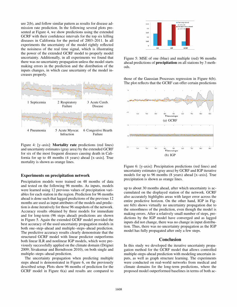
ure 2(b), and follow similar pattern as results for disease ad-mission rate prediction. In the following several plots pre-sented at Figure 4, we show predictions using the extendedGCRF with their confidence intervals for the top six killingdiseases in California for the period of 2003–2011. In allexperiments the uncertainty of the model rightly reflectedthe noisiness of the real time signal, which is illustratingthe power of the extended GCRF model to properly modeluncertainty. Additionally, in all experiments we found thatthere was no uncertainty propagation unless the model startsmaking errors in the prediction and the distribution of theinputs changes, in which case uncertainty of the model in-creases properly.

1 Septicemia 2 RespiratoryFailure

3 Acute Cereb.Disease

4 Pneumonia 5 Acute Myocar.Infraction

6 Congestive HearthFailure

Figure 4: [y–axis]: Mortality rate predictions (red lines)and uncertainty estimates (gray area) by the extended GCRFfor six of the most frequent diseases causing death in Cali-fornia for up to 48 months (4 years) ahead [x–axis]. Truemortality is shown as orange lines.

Experiments on precipitation network

Precipitation models were trained on 48 months of dataand tested on the following 96 months. As inputs, modelswere learned using 12 previous values of precipitation vari-ables for each station in the region. Prediction for 96 monthsahead is done such that lagged predictions of the previous 12months are used as input attributes of the models and predic-tion is done iteratively for those 96 snapshots of the network.Accuracy results obtained by three models for immediateand for long-term (96 steps ahead) predictions are shownin Figure 5. Again the extended GCRF model provided thebest accuracy of the used uncertainty propagation models inboth one–step–ahead and multiple–steps–ahead prediction.The predictive accuracy results clearly demonstrate that thestructured GCRF model with linear predictor outperformsboth linear ILR and nonlinear IGP models, which were pre-viously successfully applied on the climate domain (Drignei2009; Sivakumar and Berndtsson 2010), on both single andmultiple–steps–ahead prediction.

The uncertainty propagation when predicting multiplesteps ahead is demonstrated in Figure 6, on the previouslydescribed setup. Plots show 96 months of prediction for theGCRF model in Figure 6(a) and results are compared to

Figure 5: MSE of one (blue) and multiple (red) 96 monthsahead predictions of precipitation on all stations by 3 meth-ods.

those of the Gaussian Processes regression in Figure 6(b).The plot reflects that the GCRF can offer certain predictions

(a) GCRF

(b) IGP

Figure 6: [y-axis]: Precipitation predictions (red lines) anduncertainty estimates (gray area) by GCRF and IGP iterativemodels for up to 96 months (8 years) ahead [x–axis]. Trueprecipitation is shown as orange lines.

up to about 30 months ahead, after which uncertainty is ac-cumulated on the displayed station of the network. GCRFalso accurately highlights areas with larger error across theentire predictive horizon. On the other hand, IGP in Fig-ure 6(b) shows virtually no uncertainty propagation due tothe smoothness of the prediction, even though the model ismaking errors. After a relatively small number of steps, pre-dictions by the IGP model have converged and as laggedinputs did not change, there was no change in input distribu-tion. Thus, there was no uncertainty propagation as the IGPmodel has fully propagated after only a few steps.

Conclusion

In this study we developed the iterative uncertainty propa-gation method for the GCRF model that allows controlledmultiple-steps-ahead prediction with modeling uncertain in-puts, as well as graph structure learning. The experimentswere conducted on real-world networks from medical andclimate domains for the long-term predictions, where theproposed model outperformed baselines in terms of both ac-

1608

curacy and uncertainty propagation. The proposed method isalso readily applicable to other long-term structured regres-sion models with Gaussian canonical form and for applica-tions where correlation among outputs carries information.

Acknowledgments

The authors gratefully acknowledge the support of DARPAgrant FA9550-12-1-0406 negotiated by AFOSR, NSF BIG-DATA grant 14476570 and ONR grant N00014-15-1-2729.

References

Bengio, Y. 2012. Practical recommendations for gradient-based training of deep architectures. In Neural Networks:Tricks of the Trade. Springer. 437–478.Candela, J. Q.; Girard, A.; Larsen, J.; and Rasmussen,C. E. 2003. Propagation of uncertainty in bayesian kernelmodels-application to multiple-step ahead forecasting. InAcoustics, Speech, and Signal Processing, 2003. Proceed-ings.(ICASSP’03). 2003 IEEE International Conference on,volume 2, II–701. IEEE.Dey, S.; Gyorgy, J.; B.L., W.; Steinbach, M.; and Kumar, V.2014. Mining interpretable and predictive diagnosis codesfrom multi-source electronic health records. In SIAM Inter-national Conference on Data Mining.Dokic, T.; Dehghanian, P.; Chen, P.-C.; Kezunovic, M.;Medina-Cetina, Z.; Stojanovic, J.; and Obradovic, Z. 2016.Risk assesment of a transmission line insulation breakdowndue to lightning and sever weather. In Hawaii IntermationalConference on System Sciences, HICSS-49.Drignei, D. 2009. A kriging approach to the analysis ofclimate model experiments. Journal of agricultural, biolog-ical, and environmental statistics 14(1):99–114.Ghalwash, M. F.; Radosavljevic, V.; and Obradovic, Z. 2014.Utilizing temporal patterns for estimating uncertainty in in-terpretable early decision making. In Proceedings of the20th ACM SIGKDD international conference on Knowledgediscovery and data mining, 402–411. ACM.Girard, A.; Rasmussen, C. E.; Quinonero-Candela, J.; andMurray-Smith, R. 2003. Gaussian process priors with un-certain inputs – application to multiple-step ahead time se-ries forecasting. In Neural Information Processing Systems.Girard, A. 2004. Approximate methods for propagation ofuncertainty with Gaussian process models. Ph.D. Disserta-tion.Gligorijevic, D.; Stojanovic, J.; and Obradovic, Z. 2015.Improving confidence while predicting trends in temporaldisease networks. In 4th Workshop on Data Mining forMedicine and Healthcare, 2015 SIAM International Confer-ence on Data Mining.Kocijan, J.; Murray-Smith, R.; Rasmussen, C. E.; and Gi-rard, A. 2004. Gaussian process model based predictivecontrol. In American Control Conference. IEEE.Kocijan, J.; Girard, A.; Banko, B.; and Murray-Smith, R.2005. Dynamic systems identification with gaussian pro-cesses. Mathematical and Computer Modelling of Dynami-cal Systems 11(4):411–424.

Menne, M.; Williams, C.; and Vose, R. 2009. The us histor-ical climatology network monthly temperature data.Radosavljevic, V.; Vucetic, S.; and Obradovic, Z. 2010.Continuous conditional random fields for regression in re-mote sensing. In 19th European Conf. on Artificial Intelli-gence.Radosavljevic, V.; Vucetic, S.; and Obradovic, Z. 2014.Neural gaussian conditional random fields. In Proc. Euro-pean Conference on Machine Learning and Principles andPractice of Knowledge Discovery in Databases.Ristovski, K.; Radosavljevic, V.; Vucetic, S.; and Obradovic,Z. 2013. Continuous conditional random fields for efficientregression in large fully connected graphs. In Associationfor the Advancement of Artificial Intelligence Conference.Sivakumar, B., and Berndtsson, R. 2010. Advances in data-based approaches for hydrologic modeling and forecasting.World Scientific.Smith, R. C. 2013. Uncertainty Quantification: Theory, Im-plementation, and Applications, volume 12. SIAM.Stiglic, G.; Wang, F.; Davey, A.; and Obradovic, Z. 2014.Readmission classification using stacked regularized logisticregression models. In AMIA 2014 Annual Symposium.Stojanovic, J.; Jovanovic, M.; Gligorijevic, D.; andObradovic, Z. 2015. Semi-supervised learning for struc-tured regression on partially observed attributed graphs. InSIAM International Conference on Data Mining.Wytock, M., and Kolter, Z. 2013. Sparse gaussian condi-tional random fields: Algorithms, theory, and application toenergy forecasting. In Proc. of the 30th International Con-ference on Machine Learning (ICML-13), 1265–1273.

1609