Uncertainty in AVO –How can we measure it?Dan Hampson, Brian Russell, Hampson-Russell Software, CalgaryMaurizio Cardamone ENI E&P Division, Milan, Italy

Overview

AVO analysis has become a basic and accepted tool for bothexploration and production. In this regard, it has come along way from the early days when acceptance of themethod oscillated wildly between excessive expectationsand total rejection. Probably the biggest change that hascome about is that geophysicists now realize that AVO isjust one tool in the tool-box, providing a small but impor-tant addition to our knowledge of the prospect or reservoir.Predictions from AVO, as with all geophysical predictions,are really probability statements. When we see an AVOanomaly, we shouldn’t say “AVO shows there is gas here.”We should say: “AVO (and other factors) say there is probably gas here.” In fact, it would be very nice if wecould attach a believable numerical value to that probability.This paper describes a step in that direction.

Traditional AVO Analysis

The starting point of our analysis is what we can call“Traditional” AVO analysis. Of course, there are so manyapproaches to AVO these days that this is a little hard to pindown. But a good starting point is shown in Figure 1.

Figure 1 shows two synthetics which have been calculatedfrom the same basic well log data. The first case, shown atthe top of the figure, is the in situ oil case. The graph to theright of the synthetic shows that we can expect a smallincrease in amplitude with offset at both the top and thebase of the target zone. The Intercept, IO, and Gradient, G O,are measures of the response for this case. To create thesecond case, shown at the bottom of the figure, fluid substi-tution has been used to replace the oil with brine. Thechange in the synthetic is reflected in the new values ofIntercept, IB, and Gradient, GB. Theoretically, we can use this

March 2004 CSEG RECORDER 5

APRIL LUNCHEONApril 26, 2004

“Earth Model Complexity and Risk Description in Resource Exploration and Development”

Bill L. Abriel(Spring 2004 SEG Distinguished Lecturer)

MARCH LUNCHEONDATE: March 22, 2004TIME: 11:30 A.M. LunchLOCATION: Telus Convention Centre, CalgaryTICKETS: Lisa Eastman

Geo Tir Inc.TELEPHONE: 508-9815 or Fax: 508-9814

★ ★ ★ ★ ★ ★

F i g u re 1. A typical approach to AVO modeling, showing AVO synthetics and curves from the in-situ(top) and brine (bottom) cases after fluid replacement modeling.

Continued on Page 6

6 CSEG RECORDER March 2004

Luncheon Cont’dUncertainty in AVO – How can we measure it?Continued from Page 5

information to compare with intercept and gradient valuesfrom our real data prospect and see which category they fallinto, brine or hydrocarbon. In fact, this is the basis of thecurrently popular cross plot method (Ross, 2000), in which wecross plot the gradient against the intercept, and identify anom-alous regions on the cross plot.

But there are two immediate limitations to this procedure. Thefirst is that we have only two modeled values which depend ona very special set of well log conditions, and there is no reasonto expect the real data case to reflect exactly those conditions.The second is that we would like a numerical measure of howclosely the real data values conform to any one particularmodel condition.

Stochastic Modeling

The solution to the first limitation is to create a large number ofmodels, which reflect the variety of possible conditions we expectto encounter. This process, called Monte Carlo Simulation, is illus-trated in Figure 2.

In this process, as shown in Figure 2, we first reduce the model toa manageable level of complexity – for example, by limiting thenumber of layers. Then we specify ranges and probability distri-butions for all the variables in the layers which affect the syntheticresponse. This, of course, is the hard part upon which all the re s thinges. Once we have probability distributions, standard statis-tical analysis theory allows us to generate a large number of “re a l-izations” or possible models consistent with the assumeddistributions. From each of the models, we calculate a syntheticand measure the resulting intercept and gradient. When we plotall of these values on a cross plot, we get something like the plotshown to the right of Figure 2. Instead of a single Brine point anda single Oil point, we now have a large cluster of points for eachof the three fluid conditions which have been modeled.T h e o retically each cluster re p resents the range of possibleoutcomes which are consistent with our probability distributions.The overlap between these clusters also tells us something abouthow well we can expect AVO analysis to distinguish betweenthese conditions. (We will discuss this in more detail later. )

For our analysis, we assume the three-layer model illustrated inF i g u re 3.

The target is assumed to be a sand layer, embedded between adja-cent shales. The shales are characterized by the variables Vp, or P-wave velocity, Vs, or S-wave velocity, and density, where each ofthese variables is actually described by a probability distribution.The sand is characterized the large number of fundamental petro-physical parameters shown in Figure 4.

F i g u re 2. A schematic overview of the stochastic approach to AVO analysis.

F i g u re 3. The three layer model assumed for the analysis described in the text.

F i g u re 4. The factors that characterize the sand in Figure 3.

F i g u re 5. An example of trend analysis used to obtain statistics for one of thep a r a m e t e r s .

Continued on Page 7

March 2004 CSEG RECORDER 7

Luncheon Cont’dUncertainty in AVO – How can we measure it?Continued from Page 6

Continued on Page 8

In theory, each of the parameters shown in Figure 4 may bedescribed by a probability distribution, but in practice, many ofthe parameters are set as constants for the area. The very big taskof determining reasonable distributions for these parameters isaided by analyzing trends from wells in the area, as shown inF i g u re 5.

In Figure 5, P-wave velocity values for shale layers from a set ofwells in the area have been collected and plotted as a function ofdepth. By fitting smooth curves through the points, we can get anidea of the average (Mean) and scatter (Standard Deviation) ofshale velocities as a function of depth. Assuming a NormalDistribution, at selected depths, we can calculate the pro b a b i l i t ydistributions needed.

In practice, trend analysis from wells provides only a subset of theparameters which could be modeled. As seen in Figure 6, manyother parameters are set as constants or modeled based on best-guess estimates and experience with the are a .

Once the parameter distributions have been decided, it is as t r a i g h t - f o r w a rd computer task to perform the Monte-Carlosimulation. This process creates a large number of “re a l i z a t i o n s ” .Each realization is a complete three layer model, with somespecific value for each of the parameters. The relative occurre n c efor any particular parameter depends on the distribution wep rovided. For example, if the distribution for Vp, the P-wavevelocity of the shale, has a very large scatter or standard devia-tion, then the resulting models will have a correspondingly larg erange of shale velocities, reflecting our lack of knowledge aboutthis parameter.

In order to compare these modeled results with real data, we needto calculate an attribute, which can be measured in the AV Oanalysis. In our case, we are using Intercept and Gradient, so eachmodel is used to calculate a particular value of I and G, as shownin Figure 7:

F rom a particular realization or model, two synthetic traces arecalculated at two angles. Note that this uses the seismic waveletwhich is appropriate for the data set. From these synthetic traces,amplitudes are picked and the modeled values of I and G arecalculated. Even though we are picking the amplitude at the topof the sand, the sand thickness affects the result because of inter-f e rence from the wavelet at the base.

By performing a large number of simulations, we finally get aresult such as that shown in Figure 8.

F i g u re 8 shows all the modeled points colour-coded, dependingon whether the sand contains Brine, Oil, or Gas. From this figure ,we can see the expected clustering of Brine points nearer theorigin, with Oil and Gas points pushing further outwards. Thef i g u re also gives some idea of the relative separation of the clus-ters, indicating our ability to distinguish fluid properties usingAVO analysis for this re g i o n .

But this is just the modeled result at a single burial depth. Byusing the trend analysis, we can expect the parameter distribu-tions to change with depth, resulting in a movement of the clus-ters, as illustrated in Figure 9.

F i g u re 6. A practical summary of the method of assigning distributions to thep a r a m e t e r s .

F i g u re 7. A synthetic AVO model (right) created from a geological model (left).

F i g u re 8. The results of stochastic simulation for a particular case.

8 CSEG RECORDER March 2004

F i g u re 9 shows an example of how the distributions move aro u n dfor a particular case where the average sand and shale impedancet rends cross. At point 1, for example, where the sand impedanceis lower than the shale impedance, the corresponding cross plotshows typical Class 3 AVO behavior. On the other hand, at point3, where the trend lines cross, we get Class 2 AVO behavior. A n df i n a l l y, point 6 shows a Class 1 behavior. (For a discussion of thevarious AVO classes, refer to the original paper by Rutherfordand Williams (1989)).

Another important aspect of the distribution plot is shown inF i g u re 10.

The two graphs from Figure 10 show distributions calculatedf rom identical parameter sets, except that in the second distribu-tion, the calculated shear-wave velocity for the shales wasassumed to contain a 10% noise component. As a result, we seethe distributions broaden and overlap, indicating a higher uncer-tainty in our ability to distinguish between the fluid propertiesusing AVO analysis.

Finally, now that we have these clusters, how can we use themto evaluate AVO uncertainty numerically? The answer lies in astandard statistical algorithm, known as Bayes Theorem. This

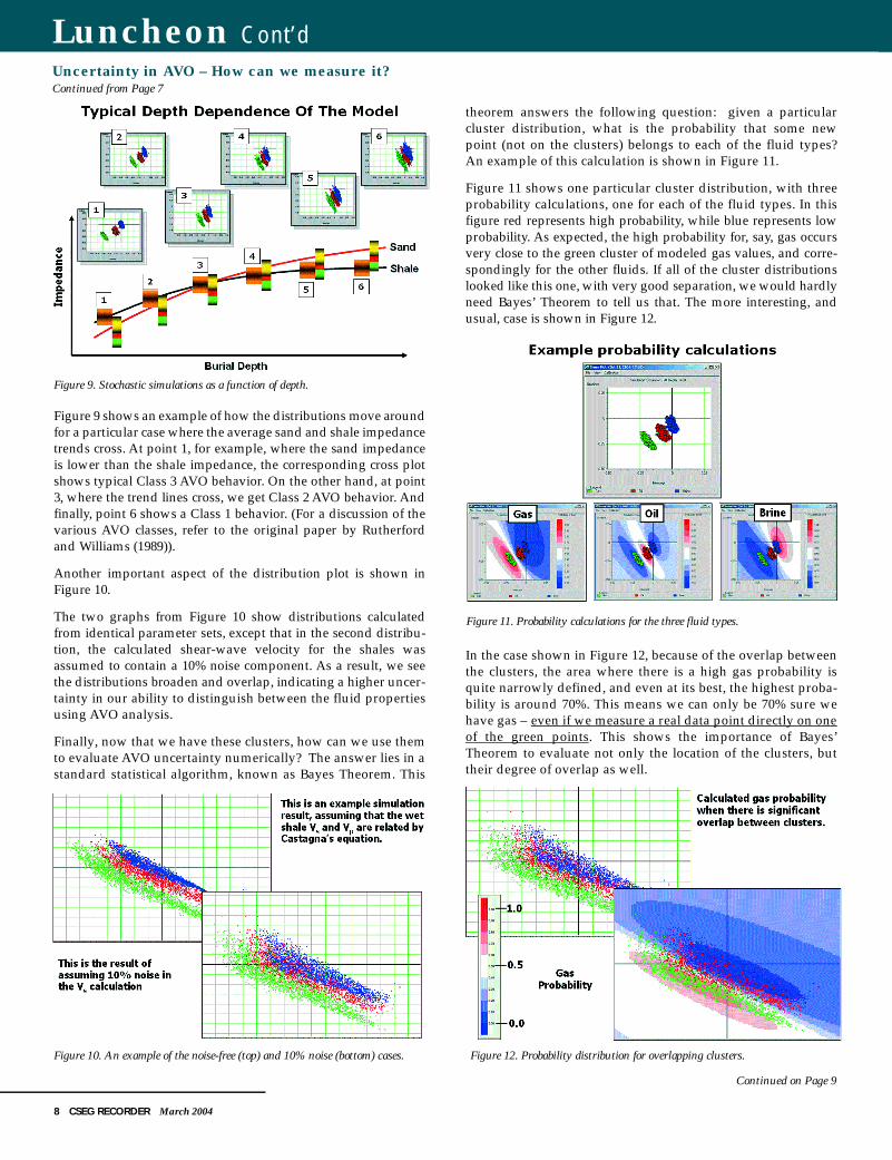
theorem answers the following question: given a particularcluster distribution, what is the probability that some newpoint (not on the clusters) belongs to each of the fluid types?An example of this calculation is shown in Figure 11.

Figure 11 shows one particular cluster distribution, with threeprobability calculations, one for each of the fluid types. In thisf i g u re red re p resents high pro b a b i l i t y, while blue re p resents lowp ro b a b i l i t y. As expected, the high probability for, say, gas occursvery close to the green cluster of modeled gas values, and corre-spondingly for the other fluids. If all of the cluster distributionslooked like this one, with very good separation, we would hard l yneed Bayes’ Theorem to tell us that. The more interesting, andusual, case is shown in Figure 12.

In the case shown in Figure 12, because of the overlap betweenthe clusters, the area where there is a high gas probability isquite narrowly defined, and even at its best, the highest proba-bility is around 70%. This means we can only be 70% sure wehave gas – even if we measure a real data point directly on oneof the green points. This shows the importance of Bayes’Theorem to evaluate not only the location of the clusters, buttheir degree of overlap as well.

Luncheon Cont’dUncertainty in AVO – How can we measure it?Continued from Page 7

F i g u re 9. Stochastic simulations as a function of depth.

F i g u re 10. An example of the noise-free (top) and 10% noise (bottom) cases.

F i g u re 11. Probability calculations for the three fluid types.

F i g u re 12. Probability distribution for overlapping clusters.

Continued on Page 9

Calibrating to the Real Data

What we have achieved so far is that we can generate pro b a b i l i t ydistributions in the Intercept/Gradient cross plots, based on pro b-ability distributions from the basic petrophysical parameters. Thisis already very useful because it allows us to estimate how wellAVO s h o u l d work in an area, if all the conditions are ideal.

The next step is to use these probability distributions to analyzeour real data results. The idea is summarized in Figure 13.

In Figure 13, the real data shown in the bottom left is a set ofmaps of Intercept and Gradient from a 3-D volume. Since weare dealing with depth trends, we may also need a map ofburial depth. By comparing these maps with the stochasticmodels, we hope to generate Fluid Probability Maps, e.g.,Probability of Gas.

In theory, this is very easy. For each point on the input maps, wecreate an Intercept/Gradient pair, find its location on thestochastic model cross plot, and read off the probability gener-ated by Bayes Theorem. Unfortunately, there is a little catch:the real data values are not scaled properly. This is becauseconventional AVO software does not extract the actual Interceptand Gradient as defined by the Zoeppritz equations, but givesan arbitrarily scaled version of these numbers, depending onthe scaling of the input seismic data. In addition to an overallscaling factor, there may also need to be an offset-dependentscaling to fix up processing problems or artifacts. We need todetermine these scalers before comparing the real data valueswith the model values.

There are many possibilities for doing this calibration betweenthe real and model data. For example, synthetic traces could becompared with the real traces and scalers found that way. Asecond possibility, which we use here, is to calibrate knownlocations on the attribute maps, as shown in Figure 14.

In Figure 14, we show two attribute maps from a 3-D pro s p e c t .The left map is the amplitude extracted at the top of the targ e tevent on the n e a r- a n g l e volume. The right map is the corre s p o n-ding amplitude map from the f a r- a n g l e volume. From these two

maps, at each grid point, we calculate Intercept and Gradient. Wealso show on the maps, six zones which have been defined forvarious reasons. The six cross plots at the lower portion of thef i g u re are the cross plots generated from the data in each of the sixzones. On these cross plots, the black dots correspond to the re a ldata Intercept/Gradient pairs, while the coloured points are theclusters calculated by stochastic modeling.

To perform the calibration between real and model cross plotvalues, we define two scalers this way:

The first scaler, SG L O BA L, multiplies both the real Intercept andGradient by the same number. This effectively accounts for theoverall global mis-match between the real and model data. Thesecond scaler, SG R A D I E N T, multiplies only the real Gradient. Thishandles the possibility that processing or other problems havecaused an amplitude imbalance between the near and far traces.

Operationally, the scalers are determined in such a way as toforce the known calibration zones to fall on the desired clusters.For example, in Figure 14, we know that zones 2, 3, and 6 are oilwells, 5 is a gas well, and zone 4 is assumed to be wet. To arriveat Figure 14, we have already adjusted the two scalers by acombination of automatic and manual calibration to achieve aconsistent overlay of all zones. We can now apply Bayes’Theorem, using these scalers, to the entire data set.

Real Data Example

As a real data example, we will show the application of thisprocedure to a 3-D data set from West Africa. The data set hasbeen processed to produce a Near Angle Stack, containing inci-dence angles from 0 to 20 degrees and a Far Angle Stack,containing angles from 20 to 40 degrees. A single inline fromeach of the stacks is shown in Figure 15.

March 2004 CSEG RECORDER 9

Luncheon Cont’dUncertainty in AVO – How can we measure it?Continued from Page 8

Continued on Page 10

F i g u re 13. A conceptual overview of the AVO fluid inversion appro a c h .

F i g u re 14. Calibration of the AVO intercept and gradient values using real dataz o n e s .

IMODEL = SGLOBAL *IREAL

GMODEL = SGLOBAL *SGRADIENT *GREAL

There are seven producing oil wells which tie the volume andproduce from the shallow formation called “A100” on Figure15. The object is to perform stochastic simulation using trendsfrom the producing wells, calibrate to the known data points,and evaluate potential drilling locations on a second deeperformation, called “A110” on Figure 15.

Using the shallow formation horizon, amplitude maps wereextracted at the seismic trough which is assumed to be the topof the productive sand. These maps are shown in Figure 16. Sixof the oil wells are also displayed on this figure. We can see asignificant increase in amplitude from near to far angles over alarge channel-like region.

Figure 17 shows an example of the trend analysis which wasperformed on the wells to determine probability distributions.This figure shows the P-wave velocity from sand layersextracted from the wells, along with the interpreted trend lines.Using similar trend analyses for the sand and shale velocitiesand densities, as well as the porosity trend analysis, parameterdistributions were established at 6 burial depths.

Figure 18 shows the result of stochastic modeling at the 6 burialdepths, using the parameters established by trend analysis. Asdiscussed previously, we can see a gradual shifting of the clus-ters from a clearly Class 3 behavior at 1400 meter depth to aclass 2 behavior at 2400 meter depth.

In Figure 19, we have selected zones around the well locationswhich we will use for calibration. In addition, we have selectedtwo large zones, which we consider to be wet. These are labeledWet Zone 1 and Wet Zone 2 on Figure 19, and are in the north-east and southwest corners of the map, away from the oil welllocations.

After manually adjusting the scaling parameters, Figure 20shows the resulting calibration at four of the selected locations.As hoped, both wet zone data points fall reasonably well on thebrine cluster, while the points from two of the oil wells fall on theoil clusters. The results for the other well locations were similar.

Using the calibration scalers in conjunction with Bayes’Theorem, we produced the oil probability map shown in Figure21. We can see that the highest probability is around 80%, even

10 CSEG RECORDER March 2004

Luncheon Cont’dUncertainty in AVO – How can we measure it?Continued from Page 9

Continued on Page 11

F i g u re 15. A single inline from the near and far stack volumes.

F i g u re 16. Amplitude slices extracted from top of producing zone.

F i g u re 17. Trend analysis for Sand P-wave velocity.

F i g u re 18. Stochastic model at 6 burial depths.

where the known oil wells are located. This reflects the uncer-tainty due to the overlap of clusters, especially at greater burialdepths. We also note that the higher oil probability trends tiethe production wells.

Finally, using the scalers and stochastic models derived fromthe shallow horizon, we apply Bayes Theorem to the deepertarget horizon. The result is shown in Figure 22. The higherprobability regions never exceed about 60%, which is probablyreasonable, given the uncertainty of the entire AVO process.Effectively, we have generated one more tool for evaluatingdrilling locations on the second horizon, which contains its ownmeasure of reliability.

Conclusions

AVO, like all geophysical measurements, is an uncertain tool.The level of uncertainty varies greatly, depending not only onthe seismic data quality, but very much on the target lithology.To enhance the credibility of the AVO process, we need to beable to quantify that uncertainty.

One way of doing that is to create probability distributions forthe underlying lithologic parameters, and derive the resulting

distributions for the seismic-derived parameters. This allows usto calculate a probability or reliability for hydrocarbon predic-tions from the seismic data.

We must be very careful, though, to recognize that the value ofthose probabilities depends completely on the accuracy of theunderlying distributions we create for the lithologic parameters.If we are going to provide uncertainty estimates along with ourAVO predictions, those estimates must be reliable themselves. R

ReferencesRoss, C. P., 2000, Effective AVO crossplot modeling : A tutorial: Geophysics, Societyof Exploration Geophysicists, 65, 700-711.

Rutherford, S. R. and Williams, R. H., 1989, Amplitude-versus-offset variations in gassands: Geophysics, Society of Exploration Geophysicists, 54, 680-688.

March 2004 CSEG RECORDER 11

Luncheon Cont’dUncertainty in AVO – How can we measure it?Continued from Page 10

F i g u re 19. Selected zones for calibration.

F i g u re 20. Calibration results, after setting scalars, at four of the selected locations.

F i g u re 21. Oil probability map generated using Bayes Theore m .

F i g u re 22. Oil probability map calculated using Bayes Theorem and scalers fro mshallow horizon.