Embed Size (px)
Citation preview

University of Nebraska - LincolnDigitalCommons@University of Nebraska - LincolnBiological Systems Engineering: Papers andPublications Biological Systems Engineering
2015
Uncertainty analysis of an irrigation schedulingmodel for water management in crop productionS. MunMississippi State University, [email protected]
G. F. SassenrathKansas State University, [email protected]
Amy M. SchmidtUniversity of Nebraska-Lincoln, [email protected]
N. LeeMississippi State University, [email protected]
M. C. WadsworthMississippi State University, [email protected]
See next page for additional authors
Follow this and additional works at: http://digitalcommons.unl.edu/biosysengfacpub
Part of the Bioresource and Agricultural Engineering Commons, Civil and EnvironmentalEngineering Commons, and the Water Resource Management Commons
This Article is brought to you for free and open access by the Biological Systems Engineering at DigitalCommons@University of Nebraska - Lincoln. Ithas been accepted for inclusion in Biological Systems Engineering: Papers and Publications by an authorized administrator ofDigitalCommons@University of Nebraska - Lincoln.
Mun, S.; Sassenrath, G. F.; Schmidt, Amy M.; Lee, N.; Wadsworth, M. C.; Rice, B.; Corbitt, Jason Q,; Schneider, J. M.; Tagert, M. L.;Pote, J.; and Prabhu, R., "Uncertainty analysis of an irrigation scheduling model for water management in crop production" (2015).Biological Systems Engineering: Papers and Publications. 345.http://digitalcommons.unl.edu/biosysengfacpub/345

AuthorsS. Mun; G. F. Sassenrath; Amy M. Schmidt; N. Lee; M. C. Wadsworth; B. Rice; Jason Q, Corbitt; J. M.Schneider; M. L. Tagert; J. Pote; and R. Prabhu
This article is available at DigitalCommons@University of Nebraska - Lincoln: http://digitalcommons.unl.edu/biosysengfacpub/345
Agricultural Water Management 155 (2015) 100–112
Contents lists available at ScienceDirect
Agricultural Water Management
jou rn al hom epage: www.elsev ier .com/ locat e/agwat
Uncertainty analysis of an irrigation scheduling modelfor water management in crop production
S. Muna, G.F. Sassenrathb, A.M. Schmidtc, N. Leea, M.C. Wadswortha, B. Ricea,J.Q. Corbittd, J.M. Schneidere, M.L. Tagerta, J. Potea, R. Prabhua,∗
a Department of Agricultural and Biological Engineering, Mississippi State University, Mississippi State, MS 39762, United Statesb Southeast Agricultural Research Center, Kansas State University, Parsons, KS 67357, United Statesc Biological Systems Engineering Department, University of Nebraska, Lincoln, NE 68583, United Statesd USDA Agricultural Research Service, Stoneville, MS 38776, United Statese WeatherSense LLC, Geary, OK 73040, United States
a r t i c l e i n f o
Article history:Received 18 September 2014Accepted 15 March 2015Available online 11 April 2015
Keywords:Irrigation schedule modelingUncertainty analysisSoil water balanceAgricultural production toolsCrop water management
a b s t r a c t
Irrigation scheduling tools are critical to allow producers to effectively manage water resources for cropproduction. To be useful, these tools need to be accurate, complete, and relatively reliable. The currentwork presents an uncertainty analysis and its results for the Mississippi Irrigation Scheduling Tool (MIST)model, showing the margin of error (uncertainty) of the resulting irrigation advice arising solely from thepropagation of measurement uncertainty through the MIST calculations. The final relative uncertainty inthe water balance value from MIST was shown to be around 9% of that value, which is in the normal rangeof the margin of error and acceptable for agronomic systems. The results of this research also indicate thataccurate measurements of irrigation and rainfall are critical to minimizing errors when using MIST andsimilar scheduling tools. While developed with data from Mississippi, the results of this uncertainty anal-ysis are relevant to similar tool development efforts across the southern and southeastern United Statesand other high-rainfall areas, especially for locations lacking high-quality co-located weather stations.
© 2015 Elsevier B.V. All rights reserved.
1. Introduction
Irrigation scheduling is a method of applying water for irrigationof crops based on calculated crop water needs. It improveswater management while maximizing crop yields. Modeling andsimulation of irrigation requirements to ensure effective watermanagement has been employed in many regions, and a num-ber of irrigation schedulers have been developed (Cancela et al.,2006; Dagdelen et al., 2006; Fortes et al., 2005; Grassini et al., 2011;Popova and Pereira, 2008). The Mississippi Irrigation SchedulingTool (MIST) was designed for the needs of producers in the Missis-sippi River Valley Alluvial Flood Plain, a region colloquially knownas the Delta (Sassenrath et al., 2013a). Continued and expanding
∗ Corresponding author. Tel.: +1 6623257351.E-mail addresses: [email protected] (S. Mun), [email protected]
(G.F. Sassenrath), [email protected] (A.M. Schmidt), [email protected](N. Lee), [email protected] (M.C. Wadsworth), [email protected] (B. Rice),[email protected] (J.Q. Corbitt), [email protected](J.M. Schneider), [email protected] (M.L. Tagert), [email protected](J. Pote), [email protected] (R. Prabhu).
reliance on ground water for irrigation by crop producers hasbegun to deplete the alluvial aquifer in the Delta, imperiling futureavailability of groundwater resources (Powers, 2007). To provideaccurate irrigation scheduling for this area, MIST uses daily weatherdata to calculate the evapotranspiration using standard equations(Allen et al., 2006), and determines daily soil water balance using acheckbook method (Andales et al., 2011).
As with all models, there are differences between in-field real-ity and model results. Simplifying assumptions useful in modelsfor one region and a specific crop are frequently not appropriatein other regions or for different crops. Therefore, it is necessaryto adjust any model to regional climate and crops, and to exam-ine the accuracy of model predictions. Several researchers haveevaluated and measured uncertainty in other irrigation schedulingsystems (Burt et al., 1997 and Molden et al., 1990), and Chaubeyet al. (1999) examined the uncertainty due to regional rainfall.Allen et al. (2011) researched common uncertainty errors aris-ing from measurements of evapotranspiration, and Snyder et al.(2015) proposed improvements on estimates of evapotranspirationto account for microclimates. Pereira et al. (2015) also investigatedand updated formulations of crop coefficients and estimates of
http://dx.doi.org/10.1016/j.agwat.2015.03.0090378-3774/© 2015 Elsevier B.V. All rights reserved.

S. Mun et al. / Agricultural Water Management 155 (2015) 100–112 101
evapotranspiration to improve accuracy. Popova et al. (2006) vali-dated their irrigation modeling system for crops and conditions inBulgaria. Prats and Picó (2010) performed a similar type of uncer-tainty analysis of the irrigation scheduling model, using aMonteCarlo method where the uncertainties of the various parameterswere considered. Monte Carlo type analysis is useful for analyzingthe statistical inference between parameters, but it is computa-tionally expensive due to the convergence test, which requiressignificant sampling from random distribution and calculation ofthe equation. Therefore, this method is difficult to use for deci-sion making tools such as an irrigation scheduling tool from apractical standpoint. On the other hand, Taylor series method, themathematical technique that we use in this manuscript, includesanalytical derivations so that the solutions can be obtained throughcomputationally inexpensive calculations.
In this study, we focused on determining the uncertainty ofMIST predictions by calculating the propagated uncertainties ofinput data through the underlying model, one aspect of overallvalidation of the MIST model. All observational data have mea-surement and observational uncertainties, and complex sequencesof calculations can in some cases result in very large uncertain-ties in the final number (prediction). Previous research examinedpotential inaccuracies in the weather database used in the waterbalance calculations and irrigation decision (Sassenrath et al.,2012), and the spatial variability of rainfall patterns (Sassenrathet al., 2013b). Uncertainty analysis quantifies the degree of errorarising from uncertainties in input data (typically measurementuncertainties) during the model calculations. The standards fordetermination of uncertainty analysis are based in quality assess-ment methodologies and guidelines developed and revised overtime by consortiums of researchers and engineers (e.g., BIPM, 2008;AIAA Standard, 1995). Coleman and Steele (2009) further refinedthe uncertainty methodology, delineating uncertainties into thosethat are caused by variability (random) and those that are not (sys-tematic), and their approach is the basis of this analysis.
Herein we examine the uncertainty in all equations and otherparameters used by MIST in the calculation of the water balance.We compare the calculated values with trends, and then evaluatethe uncertainty associated with all the parameters in the water bal-ance modeling. This gives us an indication of the sources of errorsin the measured parameters used in the daily water balance cal-culations and the contributions of the error sources to the totaluncertainty of the daily water balance. This information will be usedin subsequent studies to validate the model against soil moisturemeasurements. The following sections describe the uncertaintyanalysis methodology (Section 2), the results and discussion(Section 3) deduced from the uncertainty analysis of the MISTweb-based application, and conclusions (Section 4) of the currentresearch.
2. Methodology
2.1. Crop growth and data collection
Three crops (corn, Zea mays, cotton, Gossypium hirsutum, andsoybean, Glycine max) were grown with common production andirrigation practices, and critical data was recorded and qualityassured for use in the uncertainty calculations. Crops were grownat the USDA-ARS Mechanization Farm near Stoneville, MS from2005 to 2012 using standard agronomic practices for several dif-ferent planting dates. Plant measurements included emergencedate, growth stage, leaf area index and yield. Plant growth wasassessed as plant height and plant growth stage based on publishedstages of development; leaf area index was measured with a LAIPlant Canopy Analyzer (LiCor, Lincoln, NE). Alternatively, canopy
development was measured as percent of incoming sunlight inter-cepted by the crop canopy using a light bar (LiCor, Lincoln, NE). Yieldfrom small plots was measured at harvest by weight, and on largeplots or production farms by using yield monitors on commercialscale harvesting equipment. Soil nutrient and textural compositionwere analyzed at the Mississippi State University soil testing lab.Soil water content was measured near the rooting zone through-out the growing season using Watermark Soil Moisture Sensors(Irrometer, Inc., Irvine, CA) placed at 15 cm increments to a depthof 1 m. The Watermark sensors measure soil water tension as resis-tance changes in a solid state electrical resistance sensing deviceembedded in a granular matrix. Additional measurements weremade in production fields in 2010, 2011 and 2012 in collaborationwith cooperating producers.
Weather parameters were downloaded from the MississippiDelta Weather Center network of weather stations as previ-ously described (Sassenrath et al., 2012). Measured weatherparameters were tested for accuracy and used to calculate dailyreference evapotranspiration rates according to the modifiedPenman–Monteith method (Allen et al., 2006) in an Excel spread-sheet (Microsoft, Inc.). Crop coefficients were developed frommeasured crop growth parameters (plant height, leaf area, and per-cent light interception) as described in Sassenrath et al. (2013a)and Allen et al. (2006). The MIST daily soil water balance was deter-mined for each research and production field using a water balancemethod (Allen et al., 2006; Andales et al., 2011). All measured, cal-culated, and constant input parameters for the soil water balancecalculations are given in Table 1.
2.2. Uncertainty methodology
Uncertainties in a measured variable can arise from a varietyof sources such as an imperfect instrument calibration process,incorrect standards used for calibration, or influence on themeasured variable due to variations in ambient temperature, pres-sure, humidity and vibrations. Uncertainties can also result fromunsteadiness in an assumed “steady-state” process being mea-sured, and undesirable interactions between the transducers andenvironment (Coleman and Steele, 2009). The uncertainties thatarise due to variability or randomness of a measured quantity(such as water balance on a given day) are referred to as randomstandard uncertainty. Uncertainties that do not arise from randomvariability are called systematic standard uncertainty. The system-atic uncertainty can include calibration (bias), data acquisition, datareduction, or conceptual errors.
The systematic standard uncertainty can be calculated eitherthrough Taylor’s Series Method (TSM) or Monte-Carlo Method(MCM). With TSM, the uncertainty Ux can be calculated througha root sum of random uncertainty sx and systematic uncertainty asspecified by Coleman and Steele (2009):
Ux = √
s2x + b2
x (1)
where is the normalized deviation from the mean value for astandard Gaussian distribution.
P() = 1√2
∫
−
e−2/2d (2)
For example, for P() = 0.95 or 95% of the confidence, isapproximately 2 and for P() ≈ 0.68 or 68% of the confidence, isapproximately 1. Here, we use = 2 for 95% confidence so that thetrue value of wt, for any given day in the calculations, is expectedto lie within the bounds of 95% of the time. Similar to Eq. (1),

102 S. Mun et al. / Agricultural Water Management 155 (2015) 100–112
the uncertainty in the result is given by the following equation(Coleman and Steele, 2009):
U2r =
(∂r
∂X1
)2
U2X1
+(
∂r
∂X2
)2
U2X2
+ · · · +(
∂r
∂XJ
)2
U2XJ
(3)
where r is an experimental result, Xi are measured variables, U2Xi
arethe uncertainties in the measured variables Xi and J is the number ofmodel inputs or the measurements of the variables (temperature,humidity, etc.). This equation assumes that the measured valuesof Xi are independent of one another and the uncertainties in themeasured variables are also independent.
By dividing each term in the equation by r2, the following equa-tion is obtained from Eq. (3).
U2r
r2=(
X1
r
∂r
∂X1
)2(UX1
X1
)2
+(
X2
r
∂r
∂X2
)2(UX2
X2
)2
+ · · ·
+(
XJ
r
∂r
∂XJ
)2(UXJ
XJ
)2
which can be rearranged to give:
Ur
r=
⎛⎜⎜⎝⎛⎜⎜⎝X1
r
∂r
∂X1︸ ︷︷ ︸UMF1
⎞⎟⎟⎠
2(UX1
X1
)2
+
⎛⎜⎜⎝X2
r
∂r
∂X2︸ ︷︷ ︸UMF2
⎞⎟⎟⎠
2(UX2
X2
)2
+ · · ·
+
⎛⎜⎜⎜⎝XJ
r
∂r
∂XJ︸ ︷︷ ︸UMFJ
⎞⎟⎟⎟⎠
2(UXJ
XJ
)2
⎞⎟⎟⎟⎠
1/2
, (4)
where Ur/r is the relative uncertainty, and the factors Ux/Xi arethe relative uncertainties for each variable (Coleman and Steele,2009). The factors which multiply the relative uncertainties of
the variables are uncertainty magnification factors (UMF), and aredefined as following:
UMFi = Xi
r
∂r
∂Xi
, 1 ≤ i ≤ J (5)
The relative uncertainty is decreased when UMF is less than 1,and the relative uncertainty is increased if the value of the UMF isgreater than 1. It should be noted that the UMF are absolute values.
2.2.1. Random uncertaintyThe standard deviation of data gives an estimate of the extent of
the spread of the random uncertainty bands with a 95% confidencelevel. The assessment of the random uncertainty requires substan-tial experimentation on multiple spatial locations, and as such isnot part of this analysis.
2.2.2. Systematic uncertaintyFor this calculation, we used an estimated value of 3% of error in
each measurement as shown in Table 1, which is the standard biasof instrumentation for measuring weather parameters (Sassenrathet al., 2013b). In addition to measurement errors in weather param-eters, the systematic uncertainty in the MIST modeling procedurecould include errors from measurements of soil water, irrigationapplication rates or plant growth.
2.3. Water balance calculation
2.3.1. EvapotranspirationWe performed the uncertainty analysis on the water balance
equation for each of the measured input parameters for the calcu-lation (Table 1). The MIST equation for the water balance is basedon Allen et al. (2006), in which the net water balance of the systemis calculated from the previous water balance plus any water addedto the system less water removed from the system:
w = w(t − 1) − ETo · Kc︸ ︷︷ ︸water loss
+ Peff + I︸ ︷︷ ︸water gain
(6)
Table 1System/random uncertainty derived from climatological sensor error.
Physical quantity(unit)
Sensor/modelnumber
Data range (min,max, mean)
Accuracy (underline is chosen forthe maximum possible error)
Systematicuncertainty (br)
Random uncertainty (sr)
Wind speed(mile/day)
3-Cupanemometer/WindSentry Set 03002
(12, 202, 59.9) ±1% typical 0.01 0.03
Maximumtemperature (F)
Thermostat/VaisalaHMP45C
(33, 106, 77.3) ±0.4 C (−20 C), ±0.72 F (−4 F)±0.3 C (0 C),±0.54 F (32 F)±0.2 C (20 C), ±0.36 F (68 F)±0.3 C (40 C),±0.54 F (104 F)
(0.54/TF ,0.3/TC ,0.3/TK)a
0.03
Minimumtemperature (F)
Thermostat/VaisalaHMP45C
(23, 83, 55.9)
Solar radiation(langley/day)
Pyranometer/LI200X (15, 722, 406.2) ±5% maximum±3% typical
0.05 0.03
Maximum relativehumidity (%)
Relative humiditysensor/VaisalaHMP45C
(71, 100, 93) At 20 C:±2% (0–90% RH);±3% (90–100% RH)Dependence:±0.05% RH/C (40 C or 0 C:20 × 0.05 = ±1%)Total: 3 + 1 = ±4%
0.04 0.03
Minimum relativehumidity (%)
Relative humiditysensor/VaisalaHMP45C
(14, 97, 46.2)
Precipitation(in./day)
Tipping bucket raingauge/TE525 TI,6′′orifice
(0, 2.66, 0.1) Up to 1 in./h: ±1%1–2 in./h:±0, −3%2–3 in./h: +0, −5%
0.03 0.03
a Here, we assume that the degree of uncertainty of Fahrenheit and Celsius is proportional as much as 9/5, and Celsius and Kelvin has the same degree of uncertainty dueto the same unit scale.

S. Mun et al. / Agricultural Water Management 155 (2015) 100–112 103
where w is the current day’s water balance; w(t−1) is the previousday’s water balance; Peff is effective precipitation; and I is irrigation(Allen et al., 2006). Water balance is considered to be zero whenthe soil profile is full of water; negative values indicate a waterdeficit from the reference water balance. Because the current day’ssoil water balance depends on the previous day’s water balance,the computations are iterative. The water lost from the system isassumed to occur primarily through evapotranspiration from thecrop and soil (a valid assumption during the growing season; Allenet al., 2006), given by ETo · Kc. Here, ETo is the reference evapotrans-piration from a standardized vegetated surface (commonly grass)without shortage of water, and does not depend on crop type, cropdevelopment and management practices. Kc is a crop coefficientthat varies depending on the crop type and stage of plant growth.In MIST, the reference crop evapotranspiration is calculated usingthe modified Penman–Monteith (Allen et al., 2006):
ETo = 0.408Rn + (900/(Tmean C + 273.16))u2(es − ea) + (1 + 0.34u2)
, (7)
where Rn is net radiation at the crop surface [MJ/m2/day], Tmean Cis the mean of the daily maximum (Tmax C) and minimum temper-atures (Tmin C) (Tmean C = ( Tmax C+Tmin C/2)) [C], u2 is wind speed atstandard 2 m height [m/s], es is saturation vapor pressure [kPa],ea is actual vapor pressure [kPa], is the slope of the vapor pres-sure curve [kPa/C], and is the psychrometric constant [kPa/C](0.067 at 38.71 m above sea level for Stoneville, MS). The saturationvapor pressure deficit (es − ea) is an accurate indicator of the actualevaporative capacity of the air.
The net radiation Rn, is the difference between incoming radi-ation from the sun and outgoing radiation emitted by the earth asexpressed below (Allen et al., 2006):
Rn = Rns − Rnl (8)
where Rns is the net solar radiation, and Rnl is net longwave radia-tion. The net solar radiation, Rns, is the fraction of the solar radiationthat reaches the earth’s surface and that is not reflected from thesurface (Allen et al., 2006):
Rns = (1 − ˛)Rs (9)
where is the reflection coefficient ( = 0.23 for the hypotheticalgrass reference crop), and Rs is the solar radiation. The net longwaveradiation, Rnl, is energy loss from the earth, and is calculated as(Allen et al., 2006):
Rnl =
(T4
max K + T4min K
2
)(0.34 − 0.14
√ea)(
1.35Rs
Rso− 0.35
)(10)
where is Stefan–Boltzmann constant (4.903 × 10⁻⁹ MJ/K4 m2
day), Tmax K/min K is maximum/minimum absolute temperature dur-ing the 24-h period, ea is actual vapor pressure, Rs is solar radiation,and Rso is maximum solar radiation in the clear sky at the same loca-tion. Rs/Rso is relative shortwave radiation, expressing cloudinessof the atmosphere. It should be noted that the ratio cannot exceedone, or Rs/Rso ≤ 1.0. The equation for the maximum solar radiationin the clear sky, Rso, at 38.71 m above sea level (an average for theregion of study) is calculated by Allen et al. (2006):
Rso = 0.749224(60)
Gscdr(ωs sin(ϕ) sin(ı) + cos(ϕ) cos(ı) sin(ωs)),
(11)
where Gsc is the solar constant (0.0820 MJ/m2min), dr is inverserelative distance Earth–Sun dr = 1 + 0.033 cos
(2Dc365
), ωs is sunset
hour angle in radian ωs = acos(− tan()tan(ı)), ϕ latitude in radian,ı is solar declination ı = 0.409sin(2 Dc/365 − 1.39), and Dc is thenumber of the day in the year. It should be noted that Rso is onlybased on the location and time, and is independent of climate.
Another factor contributing to the evapotranspiration calcula-tion is the vapor pressure of the atmosphere. The saturated vaporpressure is given by Allen et al. (2006):
eo(Tc) = 0.6108 · e(17.27TC /(TC +237.3)), (12)
where TC is temperature in Celsius. Due to the non-linearity of Eq.(11), the mean saturation vapor pressure es should be calculated asfollows (Allen et al., 2006):
es =(
eo(Tmax C ) + eo(Tmin C )2
)(13)
As we want to know how much water can be vaporized to the air,the actual vapor pressure should be subtracted from the saturationvapor pressure, (es − ea). The actual vapor pressure can be derivedfrom relative humidity data so that the mean of the actual vaporpressure, ea, is (Allen et al., 2006):
ea = eo(Tmin C )(RHmax/100) + eo(Tmax C )(RHmin/100)2
, (14)
where RHmax/min is maximum/minimum relative humidity. Theslope of the saturation vapor pressure curve, , representing meantemperature and mean saturation vapor pressure is given by (Allenet al., 2006):
= 4098es
(Tmean C + 237.3)2(15)
The last term to consider in the ETo calculation, wind speed at2 m, u2, is related to the transfer of heat and water vapor from theevaporating surface into the air. To standardize the wind speedmeasurement to a height of 2 m above the surface we use the equa-tion (Allen et al., 2006):
u2 = 4.87uz
ln(67.8z − 5.42)(16)
where uz is the measured wind speed at z m above ground surface(m/s), where z is height of the wind speed measurement aboveground surface in meter.
2.3.2. Crop coefficientsTo determine the crop evapotranspiration rate, a specific crop
coefficient is required. The Kc for cotton, soybeans and corn wereadjusted from published values based on from in-field measure-ments of crops during the 2005–2012 growing seasons for eachof the planting dates. The crop evapotranspiration under standardconditions, ETc, is calculated from the reference crop evapotrans-piration multiplied by the crop coefficient. Using a crop coefficient(Kc) value, an estimate of the amount of water loss for a certain cropcan be computed.
2.3.3. Water inputs – irrigation, rainfall and runoffIrrigation (I) and effective precipitation (Peff) are water gains in
the modeled system, and both can be measured. Sassenrath et al.(2013b) explored the potential variability of rainfall measurementsfrom various sources, noting that daily rainfall measurements canvary widely even across a single crop field.
Peff is the useful amount of daily rainfall reduced by the run-offof water when there is rain in excess of what the soil can retain(Kent, 1973).
Peff =
P − Q, if P > 0.7
P, else,(17)
where P is measured precipitation and Q is direct run-off which isdefined as follows.
Q = (P − 0.2S)2
(P − 0.8S)(18)

104 S. Mun et al. / Agricultural Water Management 155 (2015) 100–112
where S is maximum potential retention after run-off begins (Kent,1973), given by:
S = 1000CN
− 10, (19)
where CN is curve number (limited 0 < CN < 100). CN depends onthe soil type, tillage and condition.
CN =
⎧⎪⎪⎪⎪⎪⎪⎨⎪⎪⎪⎪⎪⎪⎩
4.2 · SR
(10 − 0.058 · SR), if
t−1∑t=t−5
Pt < 1.4
23 · SR
(10 − 0.058 · SR), if
t−1∑t=t−5
Pt > 2.0
SR, else
, (20)
Most cropped fields in the Mississippi Delta are planted instraight rows, and the soil has been tilled to a depth greater than12 in. The soil type can be commonly classified as group “C”, witha moderately high runoff potential due to slow infiltration rate,giving a value of SR = 85 Kent, 1973.
Here,t−1∑
t=t−5
Pt is the sum of the five previous days’ precipitation.
Therefore, CN is adjusted based on the soil condition with respectto the accumulated amount of rain. If the sum of previous rain isless than 1.4 in., the soil is considered “dry” and CN is decreased. Ifthere has been more than 2 in. of rain in the previous 5 days, thesoil is considered “wet” and CN is increased. Otherwise “average”conditions are assumed and the default CN is used.
2.4. Uncertainty of the water balance equation
As the water balance equations were cascaded to calculatethe daily water balance, the uncertainties were also propagatedthrough the same set of equations, which will include weather mea-surements such as cumulative wind speed, maximum/minimumair temperature, daily total solar radiation, maximum/minimumrelative humidity temperature, and daily total precipitation. Theseweather measurements potentially include both systematic andrandom error. Systematic error can be found in the accuracy ineach measurement device (Table 1). The total uncertainty of eachmeasurement with 95% confidence level is given as follows.
• Wind speed at height z (uz)
Uuz
uz= (b2
uz+ s2
uz)1/2 = 2[0.012 + 0.032]
1/2 = 0.0006 (21)
• Maximum/minimum temperature in Fahrenheit (Tmax F/min F)
UTmax F/min F
Tmax F/min F= (b2
Tmax F/min F+ s2
Tmax F/min F)1/2
= 2
[(0.54
Tmax F/min F
)2
+ 0.032
]1/2
(22)
• Solar radiation (Rs)
URs
Rs= (b2
Rs+ s2
Rs)1/2 = 2(0.052 + 0.032)
1/2 = 0.1166 (23)
• Maximum/minimum relative humidity temperature (RHmax/min)
URHmax/min
RHmax/min= (b2
RHmax/min+ s2
RHmax/min)1/2
= 2(0.042 + 0.032)1/2 = 0.1 (24)
• Precipitation (P)
UP
P= (b2
P + s2P)
1/2 = 2(0.032 + 0.032)1/2 = 0.0848 (25)
Because some terms such as temperature share the same formof the uncertainty equation, those equations are compactly rep-resented without loss in understandability, i.e., Tmax F/min F. Also,most of the measurements are taken in English units at the weatherstation, and converted to SI units such as centigrade during the cal-culation process. Therefore, we need to define the uncertainties ofthe temperatures converted to SI units.
• Maximum/minimum/mean temperature in centigrade(Tmax C/min C/mean C)
UTmax C/min C/mean C
Tmax C/min C/mean C= 2
[(0.3
Tmax C/min C/mean C
)2
+ 0.032
]1/2
(26)
• Maximum temperature in Kelvin (Tmax K/min K)
UTmax K/min K
Tmax K/min K= 2
[(0.3
Tmax K/min K
)2
+ 0.032
]1/2
(27)
These uncertainties propagate within the water balance equa-tion in MIST, giving a relative uncertainty of the final water balanceEq. (6) as follows.
Uw
w=
⎡⎢⎢⎢⎣⎛⎜⎜⎜⎝w(t−1)
w
∂w
∂w(t−1)︸ ︷︷ ︸UMF1
⎞⎟⎟⎟⎠
2(Uw(t−1)
w(t−1)
)2
+
⎛⎜⎜⎝ETo
w
∂w
∂ETo︸ ︷︷ ︸UMF2
⎞⎟⎟⎠
2⎛⎜⎜⎝UETo
ETo︸︷︷︸(29)
⎞⎟⎟⎠
2
+
⎛⎜⎜⎝Kc
w
∂w
∂Kc︸ ︷︷ ︸UMF3
⎞⎟⎟⎠
2(UKc
Kc
)2
+
⎛⎜⎜⎜⎝Peff
w
∂w
∂Peff︸ ︷︷ ︸UMF4
⎞⎟⎟⎟⎠
2⎛⎜⎜⎜⎝UPeff
Peff︸︷︷︸(39)
⎞⎟⎟⎟⎠
2
+
⎛⎜⎜⎝ I
w
∂w
∂I︸ ︷︷ ︸UMF5
⎞⎟⎟⎠
2(UI
I
)2
⎤⎥⎥⎦
1/2
, (28)
where Uw(t−1) /w(t−1), UETo /ETo, UKc /Kc , UPeff/Peff , and UI/I are the
relative uncertainty of the previous day’s water balance, thereference evapotranspiration, the crop coefficient, the effectiveprecipitation, and the irrigation, respectively. The terms pairedwith the relative uncertainty terms are UMF terms, and thereare 5 UMF terms in the water balance equation (Table 2). UMFienclosed in a bracket refers to the UMF index number in Table 2.By plugging the reduced form of the UMFs in the table and therelative uncertainty values in the equation, we can obtain therelative uncertainty of the MIST water balance. However, the rel-ative uncertainty in the equation does not have a simple solutionbecause some of the uncertainties, such as UETo /ETo and UPeff
/Peff ,have sub-equations that are cascaded with other sub-equations.To correctly determine the uncertainty, we need to include allof the equations until it reaches the relative uncertainties of theweather data. In order to refer to the relevant sub-equation, index(i) is used under the bracket. Therefore, the final uncertainty of

S. Mun et al. / Agricultural Water Management 155 (2015) 100–112 105
Table 2Uncertainty magnification factor (UMF) for water balance equation.
Target uncertainty UMF index Reduced form of UMF term Corresponding uncertainty
Uw
w
1w(t−1)
w
∂w
∂w(t−1)= w(t−1)
w
Uw(t−1)
w(t−1)
2ETo
w
∂w
∂ETo
= EToKc
w
UETo
ETo
3Kc
w
∂w
∂Kc
= KcETo
w
UKc
Kc
4Peff
w
∂w
∂Peff
= Peff
w
UPeff
Peff
5I
w
∂w
∂I= I
w
UI
I
UETo
ETo
6
ETo
∂ETo
∂=
(0.408Rn
0.408Rn + (900/(Tmean C + 273.15))u2(es − ea)− 1
+ (1 + 0.34u2)
)U
7Rn
ETo
∂ETo
∂Rn
= 0.408Rn
0.408Rn + 900
Tmean C + 273.15u2(es − ea)
URn
Rn
8TmeanC
ETo
∂ETo
∂TmeanC= −TmeanC u2(es − ea)(900/(TmeanC + 273.15)2)
0.408Rn + ((900)/(TmeanC + 273.15))u2(es − ea))
UTmeanC
TmeanC
9u2
ETo
∂ETo
∂u2= u2
((900/(Tmean C + 273.15))(es − ea)
0.408Rn + (900/(Tmean C + 273.15))u2(es − ea)− 0.34
+ (1 + 0.34u2)
)Uu2
u2
10es
ETo
∂ETo
∂es
= (u2900es/(Tmean C + 273.15))0.408Rn + (900/(Tmean C + 273.15))u2(es − ea)
Ues
es
11ea
ETo
∂ETo
∂ea= −(u2900ea)/TmeanC + 273.15)
0.408Rn + ((900/(TmeanC + 273.15)u2(es − ea))Uea
ea
U
12TmeanC
∂
∂TmeanC
= − TmeanC
TmeanC + 237.3
UTmeanC
TmeanC
13es
∂
∂es
= 1Ues
es
Ues
es
14eo(Tmax C )
es
∂es
∂eo(Tmax C )= e0(Tmax C )
e0(Tmax C ) + e0(Tmin C )
Ueo(Tmax C )
eo(Tmax C )
15eo(Tmin C )
es
∂es
∂eo(Tmin C )= e0(Tmin C )
e0(Tmax C ) + e0(Tmin C )
Ueo(Tmin C )
eo(Tmin C )
Ueo(TmaxC )eo (TmaxC )
16Tmax C
eo(Tmax C )∂eo(Tmax C )
∂Tmax C
= 4098.171Tmax C
(Tmax C + 273.3)2
UTmax C
Tmax C
Ueo(TminC )eo (TminC )
17Tmin C
eo(Tmin C )∂eo(Tmin C )
∂Tmin C
= 4098.171Tmin C
(Tmin C + 273.3)2
UTmin C
Tmin C
URn
Rn
18Rns
Rn
∂Rn
∂Rns
= Rns
Rns − Rnl
URns
Rns
19Rnl
Rn
∂Rn
∂Rnl
= − Rnl
Rns − Rnl
URnl
Rnl
URns
Rns20
Rs
Rns
∂Rns
∂Rs
= 1URs
Rs
URnl
Rnl
21Tmax K
Rnl
∂Rnl
∂Tmax K
= 4T4max K
T4max K
+ T4min K
UTmax K
Tmax K
22Tmin K
Rnl
∂Rnl
∂Tmin K
=4T4
min K
T4max K
+ T4min K
UTmin K
Tmin K
23ea
Rnl
∂Rnl
∂ea
= −0.07√
ea
0.34 − 0.14√
ea
Uea
ea
24Rs
Rnl
∂Rnl
∂Rs
= 1.35Rs
1.35Rs − 0.35Rso
URs
Rs
Uea
ea
25RHmax
ea
∂ea
∂RHmax,
eo(Tmin C )ea
∂ea
∂eo(Tmin C )= eo(Tmin C )RHmax
eo(Tmin C )RHmax + eo(Tmax C )RHmin
URHmax
RHmax,
Ueo(Tmin C )
eo(Tmin C )
26RHmin
ea
∂ea
∂RHmin,
eo(Tmax C )ea
∂ea
∂eo(Tmax C )= eo(Tmax C )RHmin
eo(Tmin C )RHmax + eo(Tmax C )RHmin
URHmin
RHmin,
Ueo(Tmax C )
eo(Tmax C )
Uu2
u227
uz
u2
∂u2
∂uz
= 1Uuz
uz
UPeff
Peff
28P
Peff
∂Peff
∂P= P
P − Q
UP
P
29Q
Peff
∂Peff
∂Q= −Q
P − Q
UQ
Q
UQ
Q30
P
Q
∂Q
∂P= P(P + 1.8S)
(P − 0.2S)(P + 0.8S)UP
P

106 S. Mun et al. / Agricultural Water Management 155 (2015) 100–112
Fig. 1. Diagram of uncertainty analysis for water balance equation.
the water balance equation is obtained through a recursive pro-cess. The entire process for the water balance equation is depictedin Fig. 1. The remaining relative uncertainty terms of the equa-tion, Uw(t−1) /w(t−1), UKc /Kc, and UI/I, do not have sub-equations.Uw(t−1) /w(t−1) is simply from the previous day’s uncertainty of thewater balance and its initial uncertainty is set to 10%, Uw(0) /w(0) =0.1. UKc /Kc is developed from a different model and is not based onthe climate measurement in this work, so UKc /Kc = 0. The uncer-tainty in the amount of water applied in an irrigation applicationhas been studied is not considered in this work, so the uncertaintyof irrigation is set to 10%, UI/I = 0.1.
As defined in Eq. (6), w results in a water balance of zero whenthere is rain or irrigation, while the excessive water is removedfrom the soil through surface run-off. Zero water balance is conve-nient to measure the reference water balance, but it may introducea numerical error when w ≈ 0 appears in the denominator in eachterm of Eq. (28). Especially during the rainy season, the whole termcauses a divide-by-zero problem so that the total uncertainty can-not have a value or excessively high value. This leads to a difficultand erroneous calculation in the uncertainty analysis. To avoid thedivide-by-zero problem, we assign UMF1−5 = 0, and henceUw/w =0 if w = 0 in the numerical implementation of the uncertaintyanalysis.
The sub-equation for UETo /ETo of the reference crop evapotrans-piration Eq. (7) is calculated similarly to the Uw/w calculation.
UETo
ETo
=
⎡⎢⎢⎣⎛⎜⎜⎝
ETo
∂ETo
∂︸ ︷︷ ︸UMF6
⎞⎟⎟⎠
2⎛⎜⎜⎝ U
︸︷︷︸(30)
⎞⎟⎟⎠
2
+
⎛⎜⎜⎝ Rn
ETo
∂ETo
∂Rn︸ ︷︷ ︸UMF7
⎞⎟⎟⎠
2⎛⎜⎜⎝ URn
Rn︸︷︷︸(34)
⎞⎟⎟⎠
2
+(
ETo
∂ETo
∂
)2(U
)2
+
⎛⎜⎜⎝Tmean C
ETo
∂ETo
∂Tmean C︸ ︷︷ ︸UMF8
⎞⎟⎟⎠
2⎛⎜⎜⎝UTmean C
Tmean C︸ ︷︷ ︸(26)
⎞⎟⎟⎠
2
+
⎛⎜⎜⎝ u2
ETo
∂ETo
∂u2︸ ︷︷ ︸UMF9
⎞⎟⎟⎠
2⎛⎜⎜⎝ Uu2
u2︸︷︷︸(26)
⎞⎟⎟⎠
2
+
⎛⎜⎜⎝ es
ETo
∂ETo
∂es︸ ︷︷ ︸UMF10
⎞⎟⎟⎠
2⎛⎜⎜⎝ Ues
es︸︷︷︸(31)
⎞⎟⎟⎠
2
+
⎛⎜⎜⎝ ea
ETo
∂ETo
∂ea︸ ︷︷ ︸UMF9
⎞⎟⎟⎠
2⎛⎜⎜⎝ Uea
ea︸︷︷︸(37)
⎞⎟⎟⎠
2⎤⎥⎥⎦1/2
(29)
where U / is the relative uncertainty of the psychrometric con-stant, and U / = 0 because is a constant that includes onlygeological information (elevation above sea level) that causesalmost no uncertainty. Also, we ignore the UMF term paired withU / . The relative uncertainty of the mean temperature in Celsius,UTmean C
/Tmean C , is already calculated in Eq. (26). Other terms arespecified next. First, U/ of the slope of the mean saturation vaporpressure curve, Eq. (15), is given as:
U
=
⎡⎢⎢⎣⎛⎜⎜⎝Tmean C
∂
∂Tmean C︸ ︷︷ ︸UMF12
⎞⎟⎟⎠
2⎛⎜⎜⎝UTmean C
Tmean C︸ ︷︷ ︸(26)
⎞⎟⎟⎠
2
+
⎛⎜⎜⎝ es
∂
∂es︸ ︷︷ ︸UMF13
⎞⎟⎟⎠
2⎛⎜⎜⎝ Ues
es︸︷︷︸(31)
⎞⎟⎟⎠
2⎤⎥⎥⎦1/2
(30)
where UTmeanC/TmeanC is in Eq. (26), and
UTmeanCTmeanC
is
Ues
es=
⎡⎢⎢⎣⎛⎜⎜⎝ eo(Tmax C )
es
∂es
∂eo(Tmax C )︸ ︷︷ ︸UMF14
⎞⎟⎟⎠
2⎛⎜⎜⎝Ueo(Tmax C )
eo(Tmax C )︸ ︷︷ ︸(32)
⎞⎟⎟⎠
2

S. Mun et al. / Agricultural Water Management 155 (2015) 100–112 107
+
⎛⎜⎜⎝ eo(Tmin C )
es
∂es
∂eo(Tmin C )︸ ︷︷ ︸UMF15
⎞⎟⎟⎠
2⎛⎜⎜⎝Ueo(Tmin C )
eo(Tmin C )︸ ︷︷ ︸(33)
⎞⎟⎟⎠
2⎤⎥⎥⎦1/2
(31)
with
Ueo(Tmax C )
eo(Tmax C )=
⎡⎢⎢⎣⎛⎜⎜⎝ Tmax C
eo(Tmax C )∂eo(Tmax C )
∂Tmax C︸ ︷︷ ︸UMF16
⎞⎟⎟⎠
2⎛⎜⎜⎝UTmax C
Tmax C︸ ︷︷ ︸(26)
⎞⎟⎟⎠
2⎤⎥⎥⎦1/2
(32)
and
Ueo(Tmin C )
eo(Tmin C )=
⎡⎢⎢⎣⎛⎜⎜⎝ Tmin C
eo(Tmin C )∂eo(Tmin C )
∂Tmin C︸ ︷︷ ︸UMF17
⎞⎟⎟⎠
2⎛⎜⎜⎝UTmin C
Tmin C︸ ︷︷ ︸(26)
⎞⎟⎟⎠
2⎤⎥⎥⎦1/2
. (33)
Second, URn /Rn of net radiation, Eq. (8), is calculated as follows:
URn
Rn=
⎡⎢⎢⎣⎛⎜⎜⎝Rns
Rn
∂Rn
∂Rns︸ ︷︷ ︸UMF18
⎞⎟⎟⎠
2⎛⎜⎜⎝URns
Rns︸︷︷︸(35)
⎞⎟⎟⎠
2
+
⎛⎜⎜⎝Rnl
Rn
∂Rn
∂Rnl︸ ︷︷ ︸UMF19
⎞⎟⎟⎠
2⎛⎜⎜⎝URnl
Rnl︸︷︷︸(36)
⎞⎟⎟⎠
2⎤⎥⎥⎦1/2
,
(34)
where
URns
Rns=
⎡⎢⎢⎣⎛⎜⎜⎝ Rs
Rns
∂Rns
∂Rs︸ ︷︷ ︸UMF20
⎞⎟⎟⎠
2⎛⎜⎜⎝ URs
Rs︸︷︷︸(23)
⎞⎟⎟⎠
2⎤⎥⎥⎦1/2
, (35)
with URs /Rs in Eq. (23) and URnl/Rnl of the net long wave radiation
Eq. (10) is represented as follows:
URnl
Rnl=
⎡⎢⎢⎣⎛⎜⎜⎝Tmax K
Rnl
∂Rnl
∂Tmax K︸ ︷︷ ︸UMF21
⎞⎟⎟⎠
2⎛⎜⎜⎝UTmax K
Tmax K︸ ︷︷ ︸(27)
⎞⎟⎟⎠
2
+
⎛⎜⎜⎝Tmin K
Rnl
∂Rnl
∂Tmin K︸ ︷︷ ︸UMF22
⎞⎟⎟⎠
2⎛⎜⎜⎝UTmin K
Tmin K︸ ︷︷ ︸(27)
⎞⎟⎟⎠
2
+
⎛⎜⎜⎝ ea
Rnl
∂Rnl
∂ea︸ ︷︷ ︸UMF23
⎞⎟⎟⎠
2⎛⎜⎜⎝ Uea
ea︸︷︷︸(37)
⎞⎟⎟⎠
2
+
⎛⎜⎜⎝ Rs
Rnl
∂Rnl
∂Rs︸ ︷︷ ︸UMF24
⎞⎟⎟⎠
2⎛⎜⎜⎝ URs
Rs︸︷︷︸(23)
⎞⎟⎟⎠
2
+(
Rso
Rnl
∂Rnl
∂Rso
)2(URso
Rso
)2
⎤⎥⎥⎦
1/2
(36)
where UTmax K/Tmax K , UTmin K
/Tmin K , and URs /Rs are already calcu-lated in Eqs. (27) and (23), respectively. We assume that URso /Rso =0 because the corresponding equation for the maximum solar radi-ation under clear-sky conditions, Eq. (11), is based on constants
and not measurements, and hence there is almost zero uncertainty.Uea /ea of the mean of the actual vapor pressure Eq. (14) is
Uea
ea=
⎡⎢⎢⎣⎛⎜⎜⎝RHmax
ea
∂ea
∂RHmax︸ ︷︷ ︸UMF25
⎞⎟⎟⎠
2⎛⎜⎜⎝URHmax
RHmax︸ ︷︷ ︸(24)
⎞⎟⎟⎠
2
+
⎛⎜⎜⎝RHmin
ea
∂ea
∂RHmin︸ ︷︷ ︸UMF26
⎞⎟⎟⎠
2⎛⎜⎜⎝URHmin
RHmin︸ ︷︷ ︸(24)
⎞⎟⎟⎠
2
+
⎛⎜⎜⎝ eo(Tmax C )
ea
∂ea
∂eo(Tmax C )︸ ︷︷ ︸UMF26
⎞⎟⎟⎠
2⎛⎜⎜⎝Ueo(Tmax C )
eo(Tmax C )︸ ︷︷ ︸(32)
⎞⎟⎟⎠
2
⎛⎜⎜⎝ eo(Tmin C )
ea
∂ea
∂eo(Tmin C )︸ ︷︷ ︸UMF25
⎞⎟⎟⎠
2⎛⎜⎜⎝Ueo(Tmin C )
eo(Tmin C )︸ ︷︷ ︸(33)
⎞⎟⎟⎠
2⎤⎥⎥⎦1/2
, (37)
where URHmax /RHmax, URHmin/RHmin, U(e0(Tmax C ))/e0(Tmax C ), and
Ueo(Tmin C )/eo(Tmin C ) are given in Eqs. (24), (32) and (33),respectively. It should be noted that the reduced form of(RHmax/ea)(∂ea/∂RHmax) and eo(Tmin C)/ea ∂ea/∂eo(Tmin C) arethe same. Also, (RHmin/ea)(∂ea/∂RHmin) and eo(Tmax C)/ea ∂ea/∂eo(Tmax C) are the same.
The last term that we need to consider in UETo /ETo is the uncer-tainty of the wind speed at 2 m height.
Uu2
u2=
⎡⎢⎢⎣⎛⎜⎜⎝ uz
u2
∂u2
∂uz︸ ︷︷ ︸UMF27
⎞⎟⎟⎠
2⎛⎜⎜⎝ Uuz
uz︸︷︷︸(21)
⎞⎟⎟⎠
2
+(
z
u2
∂u2
∂z
)2(Uz
z
)2
⎤⎥⎥⎦
1/2
(38)
where Uz/z = 0 as height z is constant over time and does not causeuncertainties.
We have found all relative uncertainty terms in UETo /ETo. Next,we need to find the terms for the effective precipitation Eq. (17) inUw/w.
UPeff
Peff=
⎡⎢⎢⎢⎣⎛⎜⎜⎜⎝ P
Peff
∂Peff
∂P︸ ︷︷ ︸UMF28
⎞⎟⎟⎟⎠
2⎛⎜⎜⎝ UP
P︸︷︷︸(25)
⎞⎟⎟⎠
2
+
⎛⎜⎜⎜⎝ Q
Peff
∂Peff
∂Q︸ ︷︷ ︸UMF29
⎞⎟⎟⎟⎠
2⎛⎜⎜⎝ UQ
Q︸︷︷︸(40)
⎞⎟⎟⎠
2⎤⎥⎥⎥⎦
1/2
,
(39)
where UP/P is the relative uncertainty of precipitation given inEq. (25), and UQ/Q is the relative uncertainty of run-off and is givenby
UQ
Q=
⎡⎢⎢⎣⎛⎜⎜⎝ P
Q
∂Q
∂P︸ ︷︷ ︸UMF30
⎞⎟⎟⎠
2⎛⎜⎜⎝ UP
P︸︷︷︸(25)
⎞⎟⎟⎠
2
+(
S
Q
∂Q
∂S
)2(US
S
)2
⎤⎥⎥⎦
1/2
, (40)
108 S. Mun et al. / Agricultural Water Management 155 (2015) 100–112
where US/S is the uncertainty of maximum potential retention Eq.(19).
US
S=[(
CN
S· ∂S
∂CN
)2(UCN
CN
)2]1/2
(41)
where UCN/CN is the uncertainty of the curve number given in Eq.(20), and UCN/CN = 0 because the curve number equation is basedon constants. The above equations were then programmed to cal-culate the uncertainty involved in the MIST estimation of the waterbalance.
3. Results and discussion
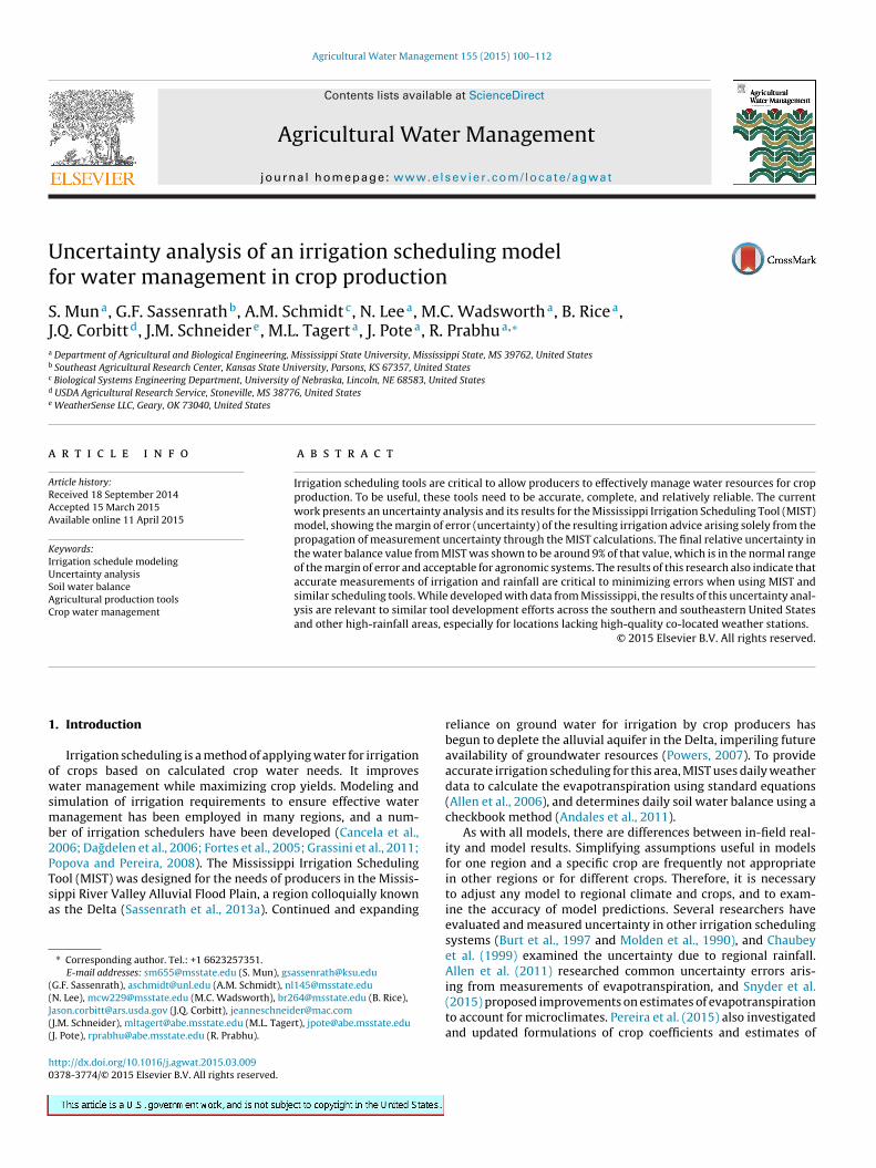
An example of the soil water balance calculation from weatherdata using an early-planted corn crop in 2012 is shown in Fig. 2.The solid blue line represents the water balance with the scaleon the right Y-axis, and the red dashed line represents the effec-tive precipitation where the run-off is subtracted with the scaleon the left Y-axis. The solid black bar indicates the one irrigationof 1.6 in. made during the 2012 season. For production agriculturein high rainfall areas such as the Mississippi Delta, heavy springrains typically eliminate the requirement for pre-planting and earlyseason irrigation applications. Research is ongoing to determineoptimal termination dates of irrigation, which will be crop specific.Therefore, we will limit our interest to the time period betweenplanting and harvesting throughout the analysis. For productionregions requiring pre-planting irrigation scheduling, modificationof the early-season water balance would be required.
The inaccuracies of sensors used for this work are listed inTable 1. As discussed in Section 2.2, UMF values help to definethe variables that influence the uncertainty equation and estimatethe amount of the influence of each variable. A UMF less than 1decreases the uncertainty of a variable, while a UMF more than1 increases the uncertainty of a variable. Fig. 3 presents the UMFsand the associated uncertainties of all of the MIST variables. Fig. 3(a)shows the 30 calculated UMF values for soybean data for a 20 dayperiod from development plotted in a 3-dimensional (3D) plot.Fig. 3(b) shows uncertainties paired with 30 UMFs (as shown in thelast column of Table 2). With the exception of the white colored barsin Fig. 3(a), most of the UMF values are less than 2. The exceptions,highlighted in white, include UMF 24 (solar radiation with respectto net longwave solar radiation (Rs/Rnl)(∂Rnl/∂Rs)), UMF 29 (relative
Fig. 2. Plot of water balance calculation results. (For interpretation of the referencesto color in text near the figure citation, the reader is referred to the web version ofthis article.)
Fig. 3. 3-Dimensional plot of early-planted corn of (a) UMF and (b) paired uncer-tainty according to 30 terms in Table 2.
uncertainty of direct run-off (Q/Peff)(∂Peff/∂Q)) and UMF 30 (pre-cipitation with respect to runoff, (P/Q)(∂Q/∂P)). Even though thevalues of UMF 24 and 30 are relatively high, the associated uncer-tainties are rather low as can been seen in the white colored barsin Fig. 3(b), resulting in an overall low uncertainty. On the otherhand, UMF 29 is very low even though the paired uncertainty ishigh; hence it prevents propagating a large error to the next stageof the uncertainty calculation. As we can see in Fig. 3(b), most of theuncertainty values are less than 10% and the uncertainty values arenot greatly influenced by the large UMFs (such as UMFs 24, 29, and30). All uncertainties from the measurement devices and assump-tions are propagated through the uncertainty equations up to thefinal uncertainty equation for the water balance, which is given inEq. (28). Therefore, UMFs and the paired uncertainties in the waterbalance uncertainty equation are important, particularly those ofw(t−1) (UMF 1), ETo (UMF 2), Peff (UMF 4) and I (UMF 5).
Fig. 4 shows the temporal changes in the UMFs of the water bal-ance uncertainty equation over the course of the growing season.There are several key points to note here. First, UMFs for w(t−1)remain close to one. This is appropriate, as the day-to-day varia-tions of the water balance and its uncertainty are usually negligible.Here the UMF for water balance is w(t−1)/w and so this ratio doesnot change much if the water balance from one day to another doesnot change much. Secondly, the UMF for w(t−1) is affected by UMFsof Peff, and I, as seen on days 158 and 163 in each sub-figure forPeff, and day 141 and 154 in subfigure (d) for I. This clearly showsthat a change in Peff or I will have a notable change in the UMF andthe uncertainty of the calculated water balance. Thus, one can infer

S. Mun et al. / Agricultural Water Management 155 (2015) 100–112 109
(a) (b)
(d)(c)
Fig. 4. UMF1,2,4,5 of (a) corn (early), (b) corn (late), (c) cotton, and (d) soybean.
that the uncertainties associated with measuring and calculatingPeff and I are high. This leads to large errors in predicting the waterbalance on days when a rainfall occurs or when the field is irri-gated. Lastly, the UMF for ETo is minimal (≈0) on most days, whichimplies that the rate of change in the water balance with respect toETo is very small, and thus, the impact of the uncertainty of ETo tothe uncertainty of water balance is minimal. This will be exploredmore completely in future research.
When the paired uncertainties (relative) of the four UMFs dis-cussed in Fig. 4 are considered (Fig. 5), they are generally low for
most of the crop season. As anticipated, Uw(t−1) /w(t−1) is immedi-ately influenced by UMFs and the uncertainties of the associatedvariables from the previous day. For instance, in Fig. 5(a) UMFs ofPeff day 163 increases the water balance uncertainty of day 165 from10% to 40%, and in Fig. 5(d) for the days 154, 158, and 163, the UMFsof Peff and I greatly affect the uncertainty of the water balance.
The uncertainties associated with Peff and I are a major con-cern for the uncertainty quantification of an irrigation schedulingprocess. Here, the high degree of spatial variability of rainfallmeans that the rainfall reported by the weather station or by
(a)
(c) (d)
(b)
Fig. 5. Paired uncertainty of UMF1,2,4,5 of (a) corn (early), (b) corn (late), (c) cotton, and (d) soybean.

110 S. Mun et al. / Agricultural Water Management 155 (2015) 100–112
(a)
(c) (d)
(b)
Fig. 6. Water balance and its uncertainty of (a) corn (early), (b) corn (late), (c) cotton, and (d) soybean for one complete growing season.
NEXRAD measurements may not reflect actual rainfall on a farmer’sfields (Sassenrath et al., 2013b). This is especially true for spa-tially diverse rains where one part of the farmer’s field may receiveheavy rain, while another part may receive no rain whatsoever.The local weather station or the NEXRAD data would report, how-ever, that the farmer’s entire field received the same amount ofrain. Additionally, farmers may not quantitatively measure theamount of irrigation water applied and hence the amount ofthe water irrigated is left to subjective speculations. The use oflocal flow meters to accurately measure the amount of waterapplied will address this potential error. Indeed, efforts are under-way to improve the metering of agricultural wells (Brandon,2014). Further, errors can arise in the irrigation application sys-tem, especially for old systems that have not been properly
maintained or measured (I. McCann, personal communication).Errors in amount of irrigation water applied through sprinklersystems can be off by more than 40% in some cases, due to miss-ing or broken sprinkler heads, and clogged or misaligned nozzles.And finally, environmental conditions (e.g., gusty winds) can leadto errors in irrigation water application from sprinkler systems(O’Shaughnessy et al., 2013). These issues lead to substantial levelsof uncertainties in measured amounts of rainfall and irrigation. Assuch, the current uncertainty analysis clearly points out the needfor a better methodology to measure local rainfall and amount ofirrigation water applied. The need for improved irrigation appli-cation systems to enhance performance of water managementhas been long recognized as a world-wide problem (Augier et al.,1995).
(a) (b)
(d)(c)
Fig. 7. Water balance over the course of one growing season with standard deviation error (a) corn (early), (b) corn (late), (c) cotton, and (d) soybean.

S. Mun et al. / Agricultural Water Management 155 (2015) 100–112 111
Finally, Fig. 6 shows the calculated water balance and the finaluncertainty of the relative water balance. The final water balanceresults showed values usually within acceptable variability rangesof around 15%. The notable exception to this is on the days wherethe water balance is close to zero. This occurs because of the highconfidence level (95%) and the numerical error in dividing-by-zeroon the days on which irrigation or precipitation occurred. Thoseuncertainties are as high as 58%. However, the plotted uncertaintyis the relative uncertainty, and the relative uncertainty depends onthe actual amount of the water balance to assess the total uncer-tainty. This becomes clearer if we look at the standard deviation(or total uncertainty) instead of the relative uncertainty and howthe uncertainty changes according to the water balance each day.Fig. 7 shows the water balance with the standard deviation of errorderived from the present uncertainty analysis. As seen, the error isbounded in a reasonable range as small as 0 in. and as large as about±0.5 in. as water balance in the soil declines below 10 in. This givesa more immediately useful range of uncertainty or error when pre-dicting the water balance. These results constitute an assessmentof the predictive accuracy of the MIST tool when used for similarcrops, soils, and climate.
4. Conclusions
In summary, the cascading equations within MIST, as speci-fied by FAO56 (Allen et al., 2006), were used to assess the totaluncertainty (equivalent to one standard deviation) of the waterbalance calculated by MIST, due to uncertainties in the input obser-vational data. Because the UMF values were primarily based onmanufacturers’ reports of instrument uncertainty, neglecting pos-sible contributions from other sources of error in observations, thisis a “best case” analysis. The following are the primary findings ofthis research:
• MIST was run and the uncertainty analyses were conducted forthree different crops (corn, cotton and soybean) with four differ-ent planting seasons and planting dates. The model predictionsof daily water balance as implemented in MIST were found to bewithin acceptable error bounds (±0.5 in.).
• The analysis illustrated how the UMFs and the associated uncer-tainties all tied into the calculation of the final water balanceuncertainty (Fig. 3). Any sudden and large increase in certainUMFs and their associated uncertainties resulted in sharplyhigher uncertainty in the water balance calculations.
• Rainfall and irrigation were by far the most significant variablesof the MIST irrigation model (Figs. 4 and 5) in impact on the modeluncertainty.
• The uncertainty in the predicted water balance due solely to mea-surement uncertainties was determined to be within acceptableranges (Fig. 6). Given more accurate local data for rainfall andirrigation, a smaller uncertainty of the MIST-predicted water bal-ance can be assured.
Acknowledgements
Support for portions of this work was received from the Missis-sippi Soybean Promotion Board and the Mississippi Corn PromotionBoard to A.M. Schmidt and G.F. Sassenrath and from MississippiState University MAFES Special Research Initiative (SRI) 2013 to R.Prabhu and G. F. Sassenrath. The authors would like to thank theDepartment of Agricultural and Biological Engineering at Missis-sippi State University for supporting this work. Special thanks andappreciation go to the cooperating farmers for the on-farm studiesof crop water use and model validation. This is contribution number15-092-J from the Kansas Agricultural Experiment Station.
Appendix A. Appendix
List of EquationsEq. (1) Total experimental uncertaintyEq. (2) Two-tailed Gaussian probabilityEq. (3) General uncertaintyEq. (4) Relative uncertaintyEq. (5) Uncertainty magnification factor (UMFi)Eq. (6) Water balance equation (w)Eq. (7) Reference crop evapotranspiration (ETo)Eq. (8) Net radiation (Rn)Eq. (9) Net solar radiation (Rns)Eq. (10) Net longwave radiation (Rnl)Eq. (11) Maximum solar radiation in the clear sky (Rso)Eq. (12) Saturation vapor pressure (eo(Tc))Eq. (13) Mean saturation vapor pressure (es)Eq. (14) Mean actual vapor pressure (ea)Eq. (15) Slope of mean saturation vapor pressure curve ()Eq. (16) Wind speed at 2 m (u2)Eq. (17) Effective precipitation (Peff)Eq. (18) Direct run-off, QEq. (19) Maximum potential retention after run-off begins, SEq. (20) Curve number, CNEq. (21) Relative uncertainty of wind speed at height z, Uuz
uz
Eq. (22) Relative uncertainty of maximum/minimum temperature in
Fahrenheit,UTmax FTmax F
,UTmin FTmin F
Eq. (23) Relative uncertainty of solar radiation,URsRs
Eq. (24) Relative uncertainty of maximum/minimum relative humidity
temperature,URHmaxRHmax
,URHminRHmin
Eq. (25) Relative uncertainty of precipitation, UPP
Eq. (26) Relative uncertainty of maximum/minimum/mean temperature in
Celsius,UTmax CTmax C
,UTmin CTmin C
,UTmean CTmean C
Eq. (27) Relative uncertainty of maximum/minimum temperature in
Kelvin,UTmax KTmax K
,UTmin KTmin K
Eq. (28) Relative uncertainty of water balance, Uww
Eq. (29) Relative uncertainty of reference crop evapotranspiration,UEToETo
Eq. (30) Relative uncertainty of slope of mean saturation vapor pressurecurve, U
Eq. (31) Relative uncertainty of mean saturation vapor pressure, Ueses
Eq. (32) Relative uncertainty of saturation vapor pressure of maximum
temperature in Celsius,Ueo (Tmax C )
eo(Tmax C )
Eq. (33) Relative uncertainty of saturation vapor pressure of maximum
temperature in Celsius,Ueo (Tmin C )
eo(Tmin C )
Eq. (34) Relative uncertainty of net radiationURnRn
Eq. (35) Relative uncertainty of net solar radiation,URnsRns
Eq. (36) Relative uncertainty of net longwave radiation,URnlRnl
Eq. (37) Relative uncertainty of mean actual vapor pressure, Ueaea
Eq. (38) Relative uncertainty of wind speed at 2 m,Uu2u2
Eq. (39) Relative uncertainty of effective precipitation,UPeffPeff
Eq. (40) Relative uncertainty of direct run-off,UQQ
Eq. (41) Relative uncertainty of maximum potential retention, USS
References
Allen, R.G., Pereira, L.S., Raes, D., Smith, M., 2006. Irrigation and Drainage Paper No.56, Crop Evapotranspiration. Food and Agriculture Organization of the UnitedNations, FAO, http://www.kimberly.uidaho.edu/water/fao56/fao56.pdf
Allen, R.G., Pereira, L.S., Howell, T.A., Jensen, M.E., 2011. Evapotranspiration informa-tion reporting: I. Factors governing measurement accuracy. Agric. Water Manag.98, 899–920.
American Institute of Aeronautics and Astronautics, 1995. Assessment of Wind Tun-nel Data Uncertainty. AIAA Standard S-071-1995. AGARD, New York.
Andales, A.A., Chavez, J.L., Bauder, T.A., 2011. Irrigation Scheduling: The WaterBalance Approach. Colorado State University Extension, Fact sheet 4.707,http://www.ext.colostate.edu/pubs/crops/04707.pdf
Augier, P., Baudequin, D., Isberie, C., 1995. The need to improve the on-farm perfor-mance of irrigation systems to apply upgraded irrigation scheduling. Irrigationscheduling: from theory to practice. In: Proceedings of the ICID/FAO Workshopon Irrigation Scheduling, Rome, Italy, 12–13 September, http://www.fao.org/docrep/w4367e/w4367e0e.htm
Bureau International des Poids et Mesures, 2008. Evaluation of Measurement Data– Guide to The Expression of Uncertainty in Measurement. GUM 1995 withminor corrections, vol. 100. JCGM, Available from: http://www.bipm.org/en/publications/guides/gum.html
112 S. Mun et al. / Agricultural Water Management 155 (2015) 100–112
Brandon, H., 2014. More Wells Need in Voluntary Metering Program. DeltaFarm Press, http://www.deltafarmpress.com/management/more-wells-need-voluntary-metering-program
Burt, C., Clemmens, A., Strelkoff, T., Solomon, K., Bliesner, R., Hardy, L., Howell, T.,Eisenhauer, D., 1997. Irrigation performance measures: efficiency and unifor-mity. J. Irrig. Drain. Eng. 123 (6), 423–442.
Cancela, J., Cuesta, T., Neira, X., Pereira, L., 2006. Modelling for improved irrigationwater management in a temperate region of Northern Spain. Biosyst. Eng. 94,151–163.
Chaubey, I., Haan, C.T., Grunwald, S., Salisbury, J.M., 1999. Uncertainty in themodel parameters due to spatial variability of rainfallI. J. Hydrol. 220,48–61.
Coleman, H.W., Steele, W.G., 2009. Experimentation, Validation, and Uncer-tainty Analysis for Engineers, third ed. John Wiley & Sons, Inc., Hoboken,NJ.
Dagdelen, N., Yılmaz, E., Sezgin, F., Gürbüz, T., 2006. Water-yield relation and wateruse efficiency of cotton (Gossypium hirsutum L.) and second crop corn (Zea maysL.) in western Turkey. Agric. Water Manag. 82, 63–85.
Fortes, P., Platonov, A., Pereira, L., 2005. GISAREG—a GIS based irrigation sched-uling simulation model to support improved water use. Agric. Water Manag. 77,159–179.
Grassini, P., Yang, H., Irmak, S., Thorburn, J., Burr, C., Cassman, K.G., 2011. High-yieldirrigated maize in the Western US Corn Belt: II. Irrigation management and cropwater productivity. Field Crops Res. 120, 133–141.
Kent, K.M., 1973. A method for estimating volume and rate of runoff in smallwatersheds Method for Estimating Volume and Rate of Runoff in Small Water-sheds. US Department of Agriculture Soil Conservation Service, SCS-TP-149,1973ftp://ftp.wcc.nrcs.usda.gov/wntsc/H&H/TRsTPs/TP149.pdf.
Gates, D.T., 1990. Performance measures for evaluation of irrigation-water-deliverysystems. J. Irrig. Drain. Eng. 116 (6), 804–823.
O’Shaughnessy, S.A., Urrego, Y.F., Evett, S.R., Colaizzi, P.D., Howell, T.A., 2013.Assessing application uniformity of a variable rate irrigtion system in a windylocation. Appl. Eng. Agric. 29, 497–510.
Pereira, L.S., Allen, R.G., Smith, M., Raes, D., 2015. Crop evapotranspirationestimation with FAO56: past and future. Agric. Water Manag. 147, 4–20,http://dx.doi.org/10.1016/j.agwat.2014.07.031.
Popova, Z., Eneva, S., Pereira, L.S., 2006. Model validation, crop coefficients and yieldresponse factors for maize irrigation scheduling based on long-term experi-ments. Biosyst. Eng. 95, 139–149.
Popova, Z., Pereira, L.S., 2008. Irrigation scheduling for furrow-irrigated maize underclimate uncertainties in the Thrace plain, Bulgaria. Biosyst. Eng. 99, 587–597.
Powers, S., 2007. Agricultural Water Use in the Mississippi Delta. Yazoo WaterManagement District, Available from: http://www.ymd.org/pdfs/wateruse/Agricultural%20Water%20Use%20Presentation.pdf
Prats, A.G., Picó, S.G., 2010. Performance evaluation and uncertainty measurementin irrigation scheduling soil–water balance approach. J. Irrig. Drain. Eng. 136(10), 732–743.
Sassenrath, G.F., Schneider, J.M., Schmidt, A.M., Silva, A.M., 2012. Quality assuranceof weather parameters for determining daily evapotranspiration in the humidgrowing environment of the Mid-South. J. Mississippi Acad. Sci. 57, 178–192.
Sassenrath, G.F., Schmidt, A.M., Schneider, J.M., Tagert, M.L., Corbitt, J.Q., van Riessen,H., Crumpton, J., Rice, B., Thornton, R., Prabhu, R., Pote, J., Wax, C., 2013a. Devel-opment of the Mississippi irrigation scheduling tool – MIST. In: ASABE AnnualInternational Meeting Paper No. 1619807, Kansas City, MO, July 21–24.
Sassenrath, G.F., Schneider, J.M., Schmidt, A.M., Corbitt, J.Q., Halloran, J.M., Prabhu,R., 2013b. Testing gridded NWS 1-day observed precipitation analysis in a dailyirrigation scheduler. Agric. Sci. 4, 621–627.
Snyder, R., Pedras, C., Montazar, A., Henry, J., Ackley, D., 2015. Advances in ET-based landscape irrigation management. Agric. Water Manag. 147, 187–197,http://dx.doi.org/10.1016/j.agwat.2014.07.024.