Uncertainty analysis in groundwater modelling projects · 2020. 9. 3. · Uncertainty quantification approaches 1. Scenario analysis with subjective probability •predefined perturbations

Uncertainty analysis in groundwater modelling projectsLuk PeetersICEWaRM webinar 19 July 2018

DEEP EARTH IMAGING FUTURE SCIENCE PLATFORM

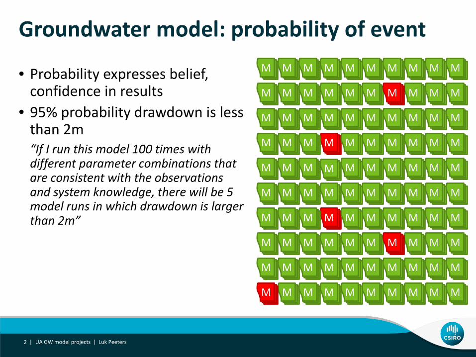
Groundwater model: probability of event

• Probability expresses belief, confidence in results

• 95% probability drawdown is less than 2m“If I run this model 100 times with different parameter combinations that are consistent with the observations and system knowledge, there will be 5 model runs in which drawdown is larger than 2m”

UA GW model projects | Luk Peeters2 |

Groundwater management

• Decision making under uncertainty• future event we want / want not to happen• risk = f( probability, consequence )

• Example 1:• event: 2m drawdown at (x,y)• consequence: bore runs dry• acceptable probability: 20%

• Example 2:• event: 2m drawdown at (x,y)• consequence: GDE disappears• acceptable probability: 1%


ProbabilityCo

nseq

uenc

e1 5 20

bore

GDE

OK

not OK

Probability of event: groundwater model

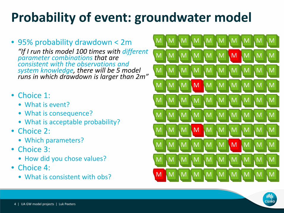
• 95% probability drawdown < 2m“If I run this model 100 times with different parameter combinations that are consistent with the observations and system knowledge, there will be 5 model runs in which drawdown is larger than 2m”

• Choice 1:• What is event?• What is consequence?• What is acceptable probability?

• Choice 2: • Which parameters?

• Choice 3: • How did you chose values?

• Choice 4: • What is consistent with obs?


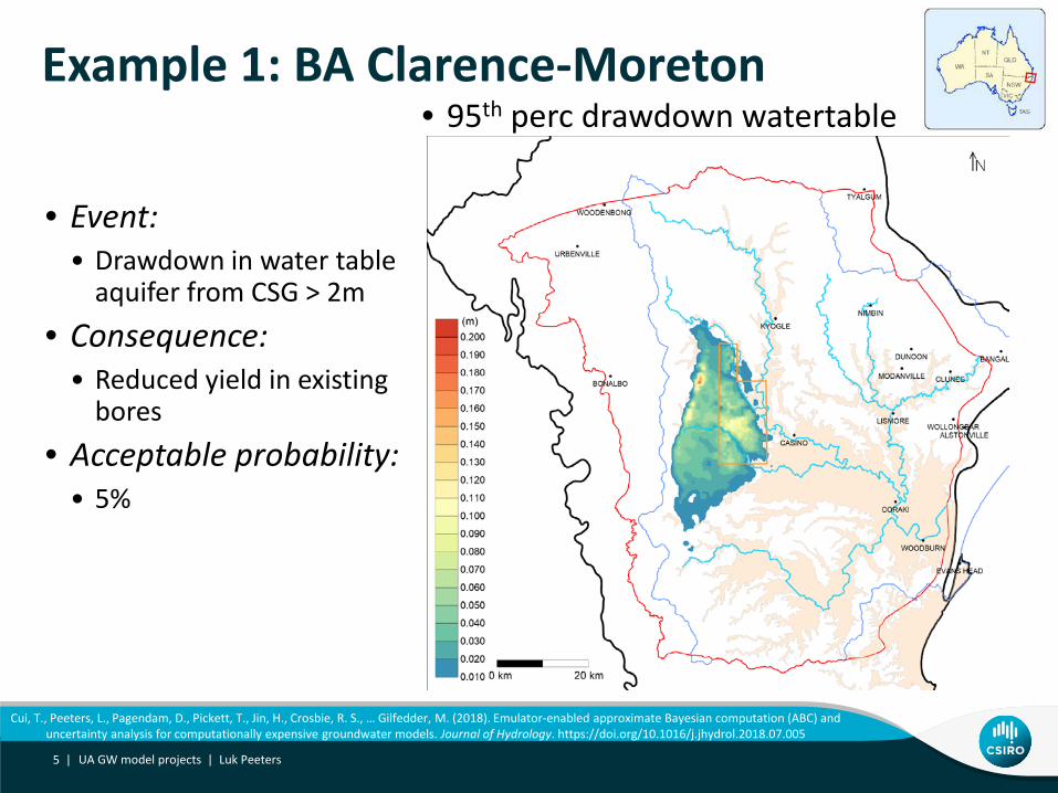
Example 1: BA Clarence-Moreton

• Event:• Drawdown in water table

aquifer from CSG > 2m• Consequence:

• Reduced yield in existing bores

• Acceptable probability:• 5%


Cui, T., Peeters, L., Pagendam, D., Pickett, T., Jin, H., Crosbie, R. S., … Gilfedder, M. (2018). Emulator-enabled approximate Bayesian computation (ABC) and uncertainty analysis for computationally expensive groundwater models. Journal of Hydrology. https://doi.org/10.1016/j.jhydrol.2018.07.005

• 95th perc drawdown watertable

Model development


Model

Geo

met

ryPr

oper

ties

Boun

dary

Cond

ition

s

HistoricalObservations

ProfessionalJudgement

QUANTITATIVE UNCERTAINTY ANALYSIS

QUALITATIVE UNCERTAINTY ANALYSIS

Peeters, L. J. M. (2017). Assumption Hunting in Groundwater Modeling: Find Assumptions Before They Find You. Groundwater, 55(5), 665–669. https://doi.org/10.1111/gwat.12565

Predictionof event

Uncertainty quantification approaches

1. Scenario analysis with subjective probability

• predefined perturbations of parameters• # model runs < # parameters

2. Deterministic modelling with linear uncertainty quantification

• model behaves linear close to calibrated values• normal with mean equal to calibrated value• >2 model runs per parameter

3. Stochastic with Bayesian uncertainty quantification

• ensemble of parameter values• >10 model runs per parameter

7 |

NU

MB

ER

OF

MO

DE

LR

UN

S

FL

EX

IBIL

ITY

TR

AN

SP

AR

EN

CY

UA GW model projects | Luk Peeters

SU

BJ

EC

TIV

EM

OD

EL

CH

OIC

ES

P+10

%

P-10

%

𝜎𝜎

𝜇𝜇

How complex to make your model and UA?

Stag

e of

inve

stig

atio

nEa

rlyLa

te

Cons

erva

tism

Com

plex

ity

Site

-spe

cific

dat

a

Probability of event

Risk

Little dataSimple model & UAVery conservative

Overestimated probabilityHigh confidence

Lots of dataComplex model & UA

Less conservativeNuanced probability

High confidence

low medium high

Schwartz, F. W., Liu, G., Aggarwal, P., & Schwartz, C. M. (2017). Naïve Simplicity: The Overlooked Piece of the Complexity-Simplicity Paradigm. Groundwater. https://doi.org/10.1111/gwat.12570

8 | UA GW model projects | Luk Peeters

Example 1: BA Clarence-Moreton

• Initial AEM, • 1,000 runs, unconstrained

• 3D MODFLOW model• Emulator-based ABC MC

Presentation title | Presenter name9 |

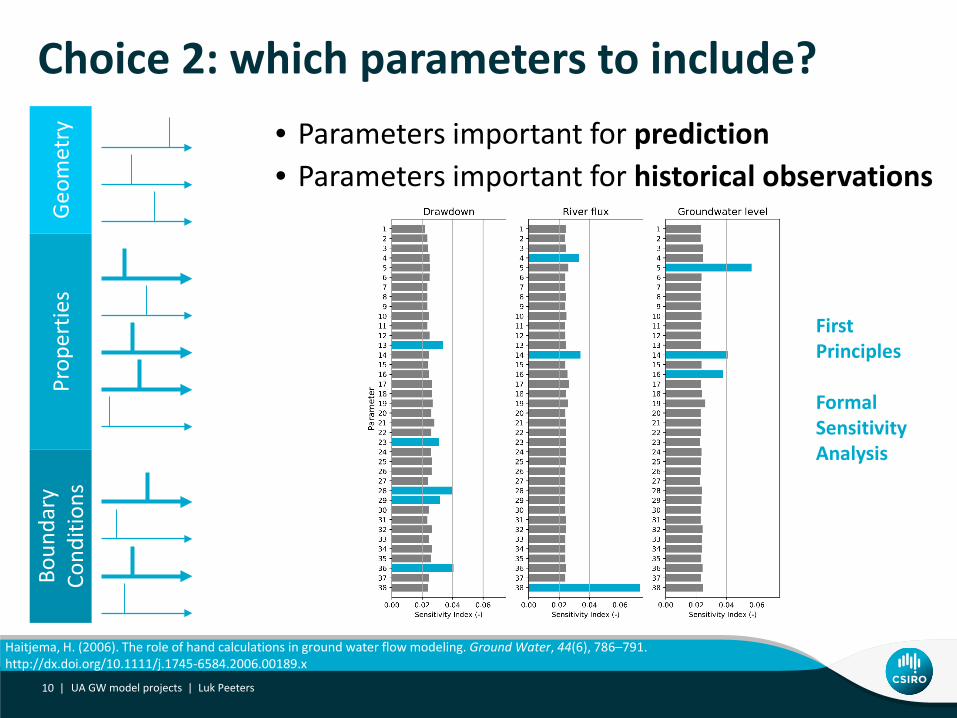
Choice 2: which parameters to include?• Parameters important for prediction• Parameters important for historical observations


Geo

met

ryPr

oper

ties

Boun

dary

Cond

ition

s

Haitjema, H. (2006). The role of hand calculations in ground water flow modeling. Ground Water, 44(6), 786–791. http://dx.doi.org/10.1111/j.1745-6584.2006.00189.x

FirstPrinciples

FormalSensitivityAnalysis

Choice 3: Prior parameter values / ranges

• Initial value or range of parameters• Strong influence on

calibration/inference• Especially important for parameters

not constrained by data• Scenario:

• subjective values (e.g. +/- 10%) • Linear:

• normal (mean, standard dev)• Stochastic:

• empirical• preference for analytic distributions

(normal, Weibull, beta, etc.)


Example: Aquitard Kv Gunnedah Basin (NSW)

12 |

Turnadge, C., Mallants, D., & Peeters L (2017). Sensitivity and uncertainty analysis of a regional-scale groundwater flow system stressed by coal seam gas extraction. CSIRO Land and Water, Adelaide. http://www.environment.gov.au/water/publications/sensitivity-and-uncertainty-analysis-regional-scale-groundwater-flow

X 50


Spatially uniform, wide range of Kv Spatially heterogeneous, wide range of Kv

Conservative Less conservative

Triangular log distribution Normal distribution with spatial covariance

Choice 4: What is consistent with data?• Good model fit:

• mismatch ≈ observation uncertainty• Observation uncertainty:

• measurement accuracy• space & time resolution

• Differencing of data (White et al. 2014)

• Scenario:• goodness-of-fit (RMSE)• professional judgement

• Linear:• minimise SE• observation weight ~ (obs unc)-1

• Stochastic:• sampling based on SE likelihood function• observation weight ~ (obs unc)-1

• Approximate Bayesian Computation / Evidential Belief Learning

13 |

h (m

asl)

time (days)


White, J. T., Doherty, J. E., & Hughes, J. D. (2014). Quantifying the predictive consequences of model error with linear subspace analysis. Water Resources Research. https://doi.org/10.1002/2013WR014767

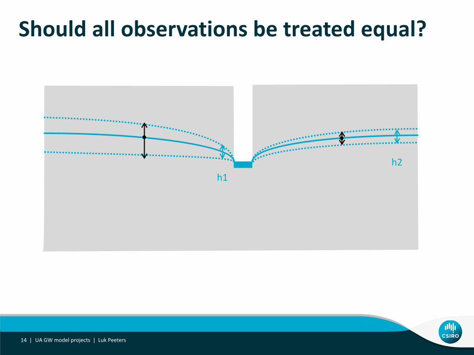
Should all observations be treated equal?

14 |

h1h2


Choice 5: How to present all this?

15 |

Peeters, L. J. M., Crosbie, R. S., Henderson, B. L., Holland, K., Lewis, S., Post, D. A., & Schmidt, R. K. (2018). The importance of being uncertain. Water E-Journal, 3(2), 10. https://doi.org/10.21139/wej.2018.018


Choice 5: How to present all this?

• No one size fits all• combine maps, tables, graphs, text

• Calibrated language • e.g. IPCC

• Reduce cognitive strain• make easy to understand• … of the 1,000 models evaluated, less

than 50 showed …• Framing

• 99% likelihood you will survive• 1% likelihood you will die


Take home messages

• Define event, consequence and acceptable probability

• 3 main UA approaches: scenario, linear, stochastic• Combine qualitative and quantitative uncertainty analysis• Common choices to document and justify

• Which parameters to include• Prior parameter values and ranges• What is deemed an acceptable model• How to present results

• Continued and intense engagement of all stakeholders


[email protected] https://research.csiro.au/dei/people/lpeeters/

DEEP EARTH IMAGING FUTURE SCIENCE PLATFORM

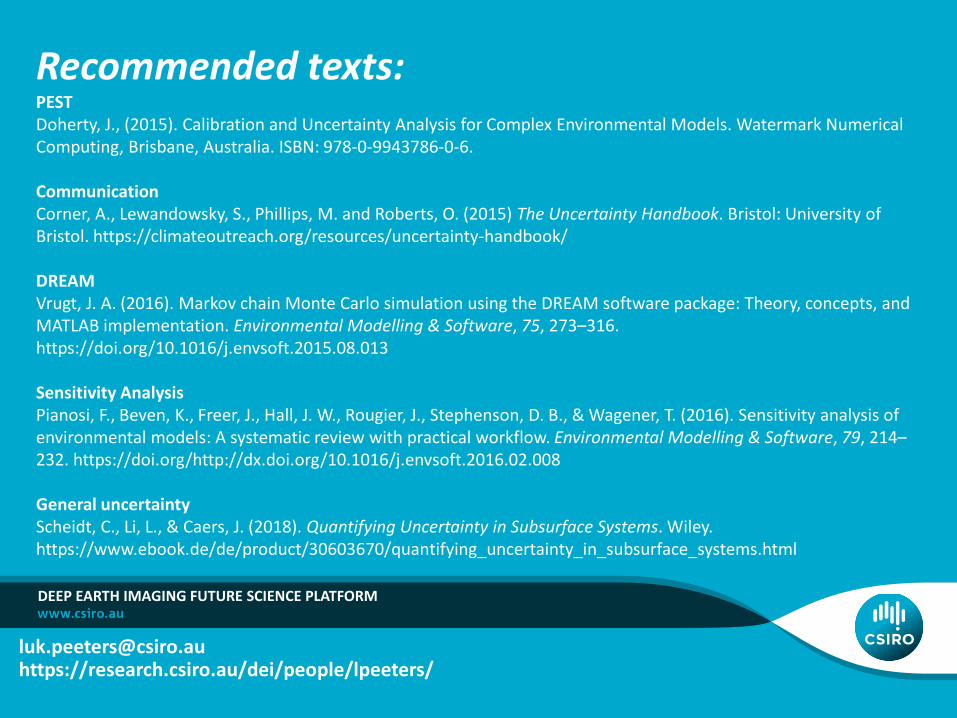
Recommended texts:PESTDoherty, J., (2015). Calibration and Uncertainty Analysis for Complex Environmental Models. Watermark Numerical Computing, Brisbane, Australia. ISBN: 978-0-9943786-0-6.

CommunicationCorner, A., Lewandowsky, S., Phillips, M. and Roberts, O. (2015) The Uncertainty Handbook. Bristol: University of Bristol. https://climateoutreach.org/resources/uncertainty-handbook/

DREAMVrugt, J. A. (2016). Markov chain Monte Carlo simulation using the DREAM software package: Theory, concepts, and MATLAB implementation. Environmental Modelling & Software, 75, 273–316. https://doi.org/10.1016/j.envsoft.2015.08.013

Sensitivity AnalysisPianosi, F., Beven, K., Freer, J., Hall, J. W., Rougier, J., Stephenson, D. B., & Wagener, T. (2016). Sensitivity analysis of environmental models: A systematic review with practical workflow. Environmental Modelling & Software, 79, 214–232. https://doi.org/http://dx.doi.org/10.1016/j.envsoft.2016.02.008

General uncertaintyScheidt, C., Li, L., & Caers, J. (2018). Quantifying Uncertainty in Subsurface Systems. Wiley. https://www.ebook.de/de/product/30603670/quantifying_uncertainty_in_subsurface_systems.html

Documents

Uncertainty analysis in groundwater modelling projects · 2020. 9. 3. · Uncertainty quantification approaches 1. Scenario analysis with subjective probability •predefined perturbations