UNCERTAINTY ANALYSIS AND INVERSION OF GEOTHERMAL CONDUCTIVE MODELS USING RANDOM SIMULATION METHODS

JARKKOJOKINEN

Institute of Geosciences

OULU 2000

UNCERTAINTY ANALYSIS AND INVERSION OF GEOTHERMAL CONDUCTIVE MODELS USING RANDOM SIMULATION METHODS

JARKKO JOKINEN

Academic dissertation to be presented with the assent of the Faculty Science, University of Oulu, for public discussion in Auditorium 4, Linnanmaa, on April 28th, 2000, at 12 noon.

OULUN YLIOPISTO, OULU 2000

Copyright © 2000Oulu University Library, 2000

Manuscript received 27 March 2000Accepted 31 March 2000

Communicated by Professor Niels Balling Professor Henry Pollack

ALSO AVAILABLE IN PRINTED FORMAT

ISBN 951-42-5590-9

ISBN 951-42-5589-5ISSN 0355-3191 (URL: http://herkules.oulu.fi/issn03553191/)

OULU UNIVERSITY LIBRARYOULU 2000

Jarkko Jokinen, Uncertainty analysis and inversion of geothermal conductivemodels using random simulation methodsGeological Survey of Finland, P.O. Box 96, FIN-02151 Espoo, FinlandActa Univ. Oul. A 343, 2000Oulu, Finland(Manuscript received 27 March, 2000)

Abstract

Knowledge of the thermal conditions in the lithosphere is based on theoretical models of heattransfer constrained by geological and geophysical data. The present dissertation focuses on theuncertainties of calculated temperature and heat flow density results and on how they depend on theuncertainties of thermal properties of rocks, as well as on the relevant boundary conditions. Due tothe high number of variables involved in typical models, the random simulation technique waschosen as the applied tool for the analysis. Further, the random simulation technique was applied ininverse Monte Carlo solutions of geothermal models. In addition to modelling techniquedevelopment, new measurements on thermal conductivity and diffusivity of middle and lowercrustal rocks in elevated pressure and temperature were carried out.

In the uncertainty analysis it was found that a temperature uncertainty of 50 K at the Moho level,which is at a 50 km’s depth in the layered model, is produced by an uncertainty of only 0.5 W m-1

K-1 in thermal conductivity values or 0.2 orders of magnitude uncertainty in heat production rate(µW m-3). Similar uncertainties are obtained in Moho temperature, given that the lower boundarycondition varies by ± 115 K in temperature (nominal value 1373 K) or ± 1.7 mW m-2 in mantleheat-flow density (nominal value 13.2 mW m-2). Temperature and pressure dependencies of thermalconductivity are minor in comparison to the above mentioned effects.

The inversion results indicated that the Monte Carlo technique is a powerful tool in geothermalmodelling. When only surface heat-flow density data are used as a fitting object, temperatures at thedepth of 200 km can be inverted with an uncertainty of 120 - 170 K. When petrologicaltemperature-depth (pressure) data on kimberlite-hosted mantle xenoliths were used also as a fittingobject, the uncertainty was reduced to 60 - 130 K. The inversion does not remove the ambiguity ofthe models completely, but it reduces significantly the uncertainty of the temperature results.

Keywords: lithosphere, heat flow, thermal regime, Monte Carlo analysis

Acknowledgements

The work was performed in the Geological Survey of Finland and it was financiallysupported by the Academy of Finland (grant 35063). This study is a contribution to theSVEKALAPKO research project, which is a part of the EUROPROBE project funded bythe European Science Foundation.

I express my gratitude to the Doctor Ilmo Kukkonen for arranging this project andversatile supervised work. The extensive scientific and administrative support fromProfessor Sven-Erik Hjelt, Department of Geophysics, University of Oulu, and fromProfessor Lauri Eskola, Department of Geophysics, Geological Survey of Finland, isgratefully acknowledged.

I thank very much the pre-examiners of my dissertation for opinions and suggestionsfor improvement. The manuscript was officially pre-examined by Professor HenryPollack, Department of Geological Sciences, The University of Michigan, and ProfessorNiels Balling, Department of Earth Sciences Geophysics, Aarhus Universitet.

The most impressive scientific remarks during the project have been made by KelinWang and Jörn Bartels. I would like to thank them, as well as, other reviewers ofpublications Heinrich Villinger, Vladimir ermák and Wolf Jacoby. I am grateful toChristoph Clauser, who kindly allowed me to use the SHEMAT program, which has beenthe prerequisite of this project. The most grateful thank of co-operators belongs to DoctorUlfert Seipold. Further help has been given also by Risto Puranen, Nils Gustavsson,Heikki Säävuori, Liisa Kivekäs, Pentti Hölttä and Reijo Niemelä. I want to thank themand all my other colleges for versatile and stimulating discussions.

Finally, I sincerely thank my family, Hanna and Alpi for their invaluable support andpatience during work.

Helsinki, March 2000 Jarkko Jokinen

List of the original articles

I Jokinen J & Kukkonen IT (1999a) Random modelling of the lithospheric thermalregime: forward simulations applied in uncertainty analysis. Tectonophysics 306 (3-4): 277–292.

II Kukkonen IT, Jokinen J & Seipold U (1999) Temperature and pressure dependenciesof thermal transport properties of rocks: Implications for uncertainties in thermallithosphere models and new laboratory measurements of high-grade rocks in theCentral Fennoscandian Shield. Surveys in Geophysics 20: 33–59.

III Jokinen J and Kukkonen IT (1999b) Inverse simulation of the lithospheric thermalregime using the Monte Carlo method. Tectonophysics 306 (3-4): 293–310.

IV Jokinen J & Kukkonen IT (2000) Inverse Monte Carlo simulation of the lithosphericthermal regime in the Fennoscandian Shield using xenolith-derived mantle tempera-tures. Journal of Geodynamics 29: 71–85.

Contents

AbstractAcknowledgementsList of the original articles1. Introduction . . . . . . . . . . . . . . . . . . . . . . . . . . . . . . . . . . . . . . . . . . . . . . . . . . . . . . . . 112. Heat transfer . . . . . . . . . . . . . . . . . . . . . . . . . . . . . . . . . . . . . . . . . . . . . . . . . . . . . . . 13

2.1. Conductive heat transfer . . . . . . . . . . . . . . . . . . . . . . . . . . . . . . . . . . . . . . . . . . . 132.2. Convective heat transfer . . . . . . . . . . . . . . . . . . . . . . . . . . . . . . . . . . . . . . . . . . . 162.3. Thermal conductivity . . . . . . . . . . . . . . . . . . . . . . . . . . . . . . . . . . . . . . . . . . . . . 17

3. Introduction to the Monte Carlo simulation and related methods . . . . . . . . . . . . . . . 213.1. Parameter sampling . . . . . . . . . . . . . . . . . . . . . . . . . . . . . . . . . . . . . . . . . . . . . . 233.2. Annealing process . . . . . . . . . . . . . . . . . . . . . . . . . . . . . . . . . . . . . . . . . . . . . . . 243.3. Metropolis algorithm . . . . . . . . . . . . . . . . . . . . . . . . . . . . . . . . . . . . . . . . . . . . . 263.4. Random walk algorithms . . . . . . . . . . . . . . . . . . . . . . . . . . . . . . . . . . . . . . . . . . 283.5. Cooling schedule . . . . . . . . . . . . . . . . . . . . . . . . . . . . . . . . . . . . . . . . . . . . . . . . 29

4. Application in the present study . . . . . . . . . . . . . . . . . . . . . . . . . . . . . . . . . . . . . . . . 315. Publications . . . . . . . . . . . . . . . . . . . . . . . . . . . . . . . . . . . . . . . . . . . . . . . . . . . . . . . . 34

5.1. Paper I . . . . . . . . . . . . . . . . . . . . . . . . . . . . . . . . . . . . . . . . . . . . . . . . . . . . . . . . 345.2. Paper II . . . . . . . . . . . . . . . . . . . . . . . . . . . . . . . . . . . . . . . . . . . . . . . . . . . . . . . . 355.3. Paper III . . . . . . . . . . . . . . . . . . . . . . . . . . . . . . . . . . . . . . . . . . . . . . . . . . . . . . . 365.4. Paper IV . . . . . . . . . . . . . . . . . . . . . . . . . . . . . . . . . . . . . . . . . . . . . . . . . . . . . . . 36

6. Discussion and conclusions . . . . . . . . . . . . . . . . . . . . . . . . . . . . . . . . . . . . . . . . . . . . 387. References . . . . . . . . . . . . . . . . . . . . . . . . . . . . . . . . . . . . . . . . . . . . . . . . . . . . . . . . . 41

1. Introduction

The major aim of geothermal modelling is to present the internal temperature and heat-flow density distribution of a studied area. Temperature and heat transfer are involved inpractically all geological and geophysical processes of the earth. For instance, whentemperature decreases, melted rocks and minerals crystallize, the deformation of therocks change from ductile to brittle, and the physical and chemical characteristics ofgeological materials vary accordingly. Actually, mantle convection and plate tectonics areexpressions of heat transfer from the hot interior of the earth to its cool surface. It is thisthermally driven system that initiates most of the fundamental geological processes andphenomena.

Our understanding of the internal thermal regime of the earth is based mainly on threefactors: firstly, on direct measurements, secondly, on geological observations and thirdly,on geophysical modelling. The direct measurements include measuring drillholetemperatures, heat production rates of rocks and heat transport properties of rocks.Thermal transport property measurements are made in surface conditions, but also inelevated temperature and pressure conditions in specialized laboratories.

In this study, the attention is focused on geothermal models, their uncertainty analysisand inverse solutions. Traditionally, forward modelling has been used in geothermalstudies. After deciding on the values of appropriate boundary conditions and thermalparameters, the temperature and heat flow values in the subsurface are calculated bysolving the involved heat transfer equations, either analytically or numerically. However,the choice of parameter values usually involves considerable ambiguity, and the problemis further complicated by the related non-linearity, due to temperature and pressuredependencies of thermal conductivity of rocks, but often only one acceptable model ispresented as a solution. Uncertainty analyses of forward models have rarely beendiscussed in geothermics.

Inverse solution, i.e. the combinations of parameter values and boundary conditions,can be mapped by the possible random solutions satisfying the measured data ontemperature and heat-flow density. Inversion methods reduce the ‘personal bias’sometimes involved in forward modelling, and may indicate solutions not apparentotherwise. Although inversion methods are commonly used in geophysics in general,their applications in lithospheric geothermics so far have been relatively few.

12

The reason for using the Monte Carlo (MC) method can be understood to be theambiguity of geothermal models which in this respect is analogous to the travellingsalesman’s dilemma (Kirkpatrick et al. 1983). The task is to find the shortest route thatvisits all chosen sites and finally returns to the initial one. When this dilemma isconverted into a mathematical form, the total sum of distances between the target sites isto be minimized. Using the simplest MC optimization, the solution can be found byselecting a set of random routes and then choosing the best of those. When the number ofsites is small, the best route is determined by going systematically through all thepossibilities. If the number of sites (n) is larger the number of different alternativesincreases (n!) as well. Here the problem becomes more difficult because solving allpossibilities is too slow and simply running through random models is not usefulanymore. The one and only best route is no longer interesting in a case where manydifferent routes have equivalent distances with insignificantly small differences. In furthercomparison, the search is made more efficient by using previous experience whenguessing at new alternatives. Instead of indifferent allotment, the probability of a re-election of good subroute combinations is increased and respectively the probability ofpoor alternatives is decreased. In the travelling salesman’s dilemma, sites close togetherhave a high probability of becoming successive visiting sites on the route. The dilemma isthus divided into smaller ‘subproblems’ as happens also in the optimization ofgeophysical models. The most significant results are optimized first. When the changes inthe model are no longer significant, the finishing of the process becomes possible. Thevisiting sites of the travelling salesman can be replaced by geothermal or whatever modelparameters.

This dissertation is based on four independent publications given in the appendix, andcontaining the original contributions to applying MC methods in uncertainty analyses(papers I and II) and inverse solutions (papers III and IV). The dissertation synopsis firstsummarizes the general theory of heat transfer in a geological medium (Chapter 2) andthen discusses the MC method in the framework of general inversions as well as globaloptimization methods (Chapter 3). In Chapter 4, the structure of the simulations in papersI–IV is presented. The major results of the independent publications are summarized inChapter 5 and 6.

Thermal elattice conconductivheat flowrelevant pboth therConvectivproduced convectiontopographconvectioncontrollingto the Sterocks conmechanism

The condwhich has

where Q itemperatuis the surfthe thickn

2. Heat transfer

nergy is transferred in the geological medium towards a lower temperature byduction, convection or radiation. In addition to temperature difference, thermality is an important factor controlling conductive heat flow. Further, in transient problems, thermal diffusivity (or density and specific heat capacity) is aarameter. Due to the temperature dependence of lattice phonon conduction,mal conductivity and diffusivity decrease with increasing temperature.e heat transfer is controlled on the one hand by the driving forces (buoyancy)by density differences due to heat expansion of viscous rock or pore fluid (free in the mantle or in an aquifer) or, on the other, by pressure gradients due to

ically controlled variations in the ground water table (advection or forced). In addition to these, hydraulic permeability is an important material property flow velocities. Radiative heat transfer is dependent on temperature according

fan-Bolzman law. In geological media, opacity is the critical property of thetrolling the efficiency of radiation. In the following, the major heat transport

s are shortly discussed.

2.1. Conductive heat transfer

uction of heat can be presented by Fourier’s first law (Haenel et al. 1988), been derived experimentally:

, (1)

s the quantity of heat [J], λ is thermal conductivity [W m-1 K-1], T2 – T1 isre difference [K] between the two boundary surfaces of a plano parallel plate, Aace area of the plates [m2], t is the time [s] during which the heat flows and h isess of the plate [m]. The heat-flow density q for unit area and unit time is

( )h

TTQ 12 −

−=λ

dT

. (2)

dhq λ−=

This is boreholes also in thsamples. G

where q [W+ ∂T / Hamilton-and respec

Therma

where P i-(∂qz / ∂z)

IndepedV during

where ρ isheat capactime t [s].

Fourier1988)

Substit

and then ait follows

where a time-depethermal di

14

also the basic equation to be used to determine geothermal heat-flow density inwith temperature measurements at different depths for gradient estimation, ande corresponding laboratory measurements of thermal conductivity from theenerally, heat flow is three dimensional

(3)

m-2] and temperature gradient ∇T are vectors (q = (qx, qy, qz), ∇T = ∂T / ∂x∂y + ∂T / ∂z). The commonly needed differential operators are theoperator (Nabla) and the Laplace-operator, marked: ∇ = (∂ / ∂x, ∂ / ∂y, ∂ / ∂z)tively ∆ = ∇⋅∇ = (∂2 / ∂x2 + ∂2 / ∂y2 + ∂2 / ∂z2).l energy flowing through the volume dV (dx dy dz) in unit time is marked

, (4)

s power [W] and the vertical heat-flow density dqz through the plate dx dy is dV and dqx, dqy respectively. ndently of the previous equation, thermal energy flow P to the volume element unit time can be solved by equation

, (5)

the density [kg m-3], c is specific heat capacity [J kg-1 K-1], (ρc is volumetricity), dV is the volume [m3], and ∂T / ∂t is the temperature change during unit

’s second equation is developed by setting (4) and (5) equal (Haenel at al.,

. (6)

uting for q with corresponding equations:

(7)

ssuming the rock material to be isotropic and homogeneous (λx = λy = λz = λ),that

, (8)

(= λ / ρc) is thermal diffusivity [m2 s-1]. According to equation (8), a

gradTT λλ −=∇−=q

dVz

qy

q

xq

P zyxflow

∂∂

+∂

∂+

∂∂

−=

tT

cdVPstored ∂∂

= ρ

tT

cdiv∂∂

=− ρ)(q

tT

cz

zT

y

yT

xxT

zyx

∂∂

=

∂

∂∂

∂+

∂

∂∂

∂+

∂

∂∂

∂ρ

λλλ

Taz

T

y

T

x

Tct

T∆=

∂

∂+

∂

∂+

∂

∂=

∂∂

2

2

2

2

2

2

ρλ

ndent temperature change (moving of the temperature pulse) is controlled byffusivity.

Given t

where H conductivthe crust mineral re∂t = 0) eqproduction

The misotopes o(40K) (Bu

where H concentratfor potassequation uranium, t

Analytmost comvalue probCarslaw &

Tempecalculatedflow of thdensity ρ slab depedensity. Fhave beenheat-flow

and furthe

At the The first cintegrationgives

15

hat there is an internal heat generation in the medium, a new term is added

, (9)

is heat production rate [W m-3]. The temperature varies as a function ofe heat transport and heat production (or heat sink). Heat production of rocks inis primarily caused by radioactive elements, but may be present also due toactions during diagenesis and metamorphism. In a steady state condition (∂T /uation (9) is called the Poisson-equation (a ∆T + H / ρc = 0) and with no heat the rest of the formula is called the Laplace-equation (∆T = 0).

ost common sources of radiogenic heat production are natural radioactivef uranium (the decay series of 238U and 235U), thorium (232Th), and potassiumntebarth, 1984; Rybach, 1988). Heat production in rocks can be calculated as

, (10)

is heat production rate [µW m-3], ρ is density [kg m-3] and c is the totalion in ppm (parts per million) [10-6 kg kg-1] for uranium and thorium, and %ium. The 40K / K ratio is assumed to be constant. Numerical values in the(10) are the heat production constants H [W kg-1] of the decay series ofhorium, and potassium.ical solutions such as equation (9) have been widely used in geothermics. Themon types of problems are those where the equation is solved as a boundarylem with known surface temperature and mantle heat-flow density (see, e.g. Jaeger (1959) for a wealth of solutions).

rature within a layer with constant conductivity and heat production is as follows (Turcotte & Schubert, 1982). Firstly, the total increase of the heatin (infinitesimal) slab depends on the heat production rate (per unit mass) H, onand the thickness of the slab δz. Secondly, the change of heat flow in the thinnds on the thickness of the slab and on the rate of change of the heat-flowourier’s law (equations 1 and 2) has been used as Turcotte & Schubert (1982) presented. When we equalize these to describe the changing rate of thedensity, we obtain

(11)

r

. (12)

surface of a half-space z = 0, the temperature is T0 and heat-flow density is q0 .onstant of the integration is c1 = q = -q0 [W m-2] and the second constant of the is c2 = λ T = λ T0 [W m-1] on z = 0. The first integration of the equation (12)

cH

TatT

ρ+∆=

∂∂

( ) 51048.356.252.9 −++= KThU cccH ρ

−=

2

2

dz

TdzzH λδδρ

2

2

dz

TdH λρ −=

and the se

Finally

where T0 conductiv

It is colow heat psuch casesmodels byproductionz [m] candistance [mthe top bo

where h temperatucompiled

Flowing difference

where q iskg-1 K-1],temperatuDarcy vel(water) pexperimen

16

(13)

cond integration results

. (14)

, the temperature at the depth z is

, (15)

is the surface temperature, q0 is the surface heat flow density, ë is the thermality and H is the heat production rate.mmon to assume that heat production decreases with depth because the maficroduction rocks become more common with depth (Heier & Adams, 1965). For there are different possible solutions. The equation (15) can be applied to layer calculating temperatures consecutively layer by layer with different heat values from top to bottom. Alternatively, the heat production rate at the depth

be described for instance as H(z) = H0 exp(-z / d), where d is the particular] at which heat production is reduced to the value 1 / e (= 0.368) of its value at

undary (Buntebarth, 1984). Then, the solution of the equation (9) is of the form:

, (16)

is the thickness of the layer. The solutions become more complex if there dependence of the thermal conductivity is included. Such results have beene.g. by ermák & Haenel (1988).

2.2. Convective heat transfer

water transfers heat to and from the rock depending on the temperature between those two (Haenel et al., 1988). The heat transported by water flow is

, (17)

heat-flow density [W m-2], ρ is density [kg m-3], c is specific heat capacity [J vf is the Darcy velocity of fluid in a porous medium [m s-1] and T isre [K]. The index w refers to water and the index f to filtration. The so-calledocity (or pore velocity) is: vf = va P, where va is the average velocity of thearticle [m s-1], and P is the porosity of the medium [%]. The originallytally determined Darcy’s law is given by

, (18)

200 2

zH

zq

TTλ

ρλ

−+=

00

2

2TzqT

zH λλρ ++−=

0qdzdT

Hz +−= λρ

( )Tvcdivq fwwρ=

gradhkv ff =

−−+

−−+=

dzdH

dhdH

zq

zTzT exp1exp)(2

0000 λλλ

where kf stands fohorizontal

In a hocompleted

where thepropertiesmedium a

and

where P isThese

such as liaffecting hshould beBoth tempthe drill hand their eand Kukket al. (19solved alsshown.

Because oconductiodependenc

where A [phonons. phonons b

17

is the hydraulic conductivity [m s-1], the subscript f refers to flow and grad hr dimensionless hydraulic pressure gradient (water-level differences [m] / distance [m]).mogeneous and isotropic medium the equation (9) of heat transport will be by the convective part:

, (19)

subscript A refers to the average values of the medium – including the of rock and water in a saturated medium. The properties of rock, fluid, andre related:

(20)

, (21)

the porosity [%], r refers to rock and w refers to water (or gas).equations for hydrological problems can be simplified in large scale problemsthosphere geothermics. However, hydrology may have an important role ineat-flow density in drill holes (Smith & Chapman, 1983) and all disturbances

carefully removed from the data before applying them to conductive models.erature and heat-flow density are predisposed to errors owing to water flow inoles and climatic changes that have taken place over time. These phenomenaffects on the Fennoscandian Shield have been discussed for example by Jõeleht

onen (1996), Kukkonen (1988, 1995), Kukkonen & Clauser (1994), Kukkonen98), and Balling (1995). Hydrological corrections in thermal models can beo by applying pure hydrological models like Bear & Verruijt (1987) have

2.3. Thermal conductivity

f the temperature and pressure dependence of thermal conductivity, the heatn equation is a non-linear problem. A typical equation used for temperaturee of lattice (phonon) thermal conductivity is

, (22)

W-1 m K] and B [W-1 m] are constants related to the scattering properties ofAccording to Schatz & Simmons (1972) A is related to the scattering ofy impurities and imperfections, and B is related to phonon-phonon scattering.

( )TvcdivHTtT

c awwAAA ρλρ −+∆=∂∂

( ) wrA PP λλλ +−= 1

( ) wwrrAA cPcPc ρρρ +−= 1

BTA +=

1λ

Radiatitransport binto one c

where C [of the maexperimenmany othKukkonenconductedHuenges (that commthough resanisotropyquartz-rich

Seipoldthermal cdifficult tconductivintroducedparameterthe single can be for

and by inresults in instance). dependenc

RespectivA. equaticonductivbecause pu

18

ve heat transport follows the T3 -law where T = T [K]. In rocks, radiativeecomes relevant at about 1000 K. Combining lattice and radiative heat transfer

onductivity value yields

, (23)

W m-1 K-4] is a constant controlled by the refraction and extinction propertiestter (Schatz & Simmons, 1972). Due to several involved factors, laboratoryts of thermal conductivity at high temperatures can alternatively be fitted with

er types of formulas than the two previous equations (Hanley et al., 1978; & Jõeleht, 1996; Lehmann et al., 1998). Laboratory measurements have been and collected among others by Balling (1976), Clauser (1988), Clauser &1993), and Zoth & Haenel (1988). The data presented in the literature indicateson rock types show more or less similar temperature dependent behaviour evenults from individual minerals can be very different and strongly influenced by (Clauser, 1988; Clauser & Huenges, 1993). Generally, thermal conductivity of rocks decreases more rapidly with temperature than that of quartz-poor rocks. (1998) compiled the presently available data on temperature dependencies of

onductivities of different rock types fitted to the equation (22). Since it iso see the connection between the parameters A, B, and the measuredity values at elevated temperatures, a practical formulation of equation (22) is below. Instead of using parameters A and B, it is possible to use two other

s, namely thermal conductivity at a reference temperature λ0 [W m-1 K-1] andtemperature coefficient of thermal conductivity b [K-1]. The values for λ0 and bmed by equating

(24)

cluding the solution in the reference temperature: λ0 = 1 / (A + B T0) whicha = 1 + b T0 and b = B / A, where T = T [K] and T0 = 293 K = 20 °C (forJoining the parameters a and b leads to the following form of temperaturee of λ

. (25)

ely, transformations in the opposite direction are A = (λ0 (1 + b T0))-1 and B = bons (25) and (22) give identical temperature dependences of thermality. The benefit of using eq. (25) was clearly seen in the uncertainty analysisre temperature dependence could be simulated with only one parameter.

31CT

BTA+

+=λ

bTa

BTA +=

+ 11

0λ

bTbT

++

=11 0

0λλ

Table 1. Pafter Seipoarea and Calculated(20 °C). N

As shoalso λ0 anof thermaconductivwith increfact is use

Fig. 1. Coand therm

Amphibolite

Basalts

Granites

Granulites

Gneisses

Pyroxenites

Serpentinite

Olivine rock

Mafic granu

Mafic granu

19

arameters A, B, b, and λ0 of temperature dependence of thermal conductivityld (1998) and Kukkonen et al. (1999). Mafic granulites I are from the Kiuruvesi

mafic granulites II are from the Varpaisjärvi area, both in Finland (paper II). b = B / A and λ0 = 1 / (A + B T0), where T0 is the reference temperature 293 K is the number of samples.

wn by Seipold (1998) the parameters A and B are correlated, and consequentlyd b. On the basis of table 1 and fig. 1, the coefficient of temperature dependencel conductivity b increases (on the average) with an increase of thermal

ity in the reference temperature λ0. Typically, phonon conductivity decreasesasing temperature asymptotically towards the value of 1 - 2 W m-1 K-1. Thisful in case of missing data or poor knowledge about the rock type.

rrelation between coefficient b (temperature dependence of thermal conductivity)

A B*10000 b*1000 λ0 N

s 0.375 1.89 0.504 2.32 16

0.359 1.43 0.398 2.49 4

0.203 4.07 2.005 3.10 15

0.271 3.66 1.351 2.64 8

0.241 3.48 1.444 2.92 26

0.375 1.89 0.504 2.32 16

s 0.427 1.10 0.258 2.18 7

s 0.110 3.18 2.891 4.92 13

lites I 0.417 1.8 0.432 2.13 3

lites II 0.440 1.04 0.236 2.13 5

al conductivity λ0 in room temperature.

The infa pressureincreasingrises rapidas in thermthe porosithe pressuthe rising rock-formabout 12 (Seipold 1mafic higfollows thdependenc

Fig. 2. Fouequation (2

20

luence of pressure on thermal conductivity consists of two phenomena. Below value of about 100 MPa, the effect of microcracks gradually disappears with pressure (Buntebarth 1984). Due to this compression, thermal conductivityly to a more stable level. This threshold change in thermal conductivity as wellal diffusivity (Seipold 1995) can be up to several tens of percent, depending on

ty properties of the rocks. At depths greater than c. 3.4 kilometres (c. 100 MPa),re dependence of thermal conductivity increases approximately linearly withpressure due to the reduction in the intrinsic porosity and the compressibility ofing minerals. The increase in the thermal conductivity of granite is typically% GPa-1 (1 GPa corresponds to the depth of c. 34 km in the earth’s crust)995), but much smaller values are reported as well, e.g. in the new data on theh-grade rocks in paper II. The pressure dependence of thermal conductivitye function λ = λ0 (1 + a p), where a is the coefficient for the pressuree of thermal conductivity [Pa-1] and p is the pressure [Pa].

r examples on temperature dependence of thermal conductivity calculated using5).

3. Int

Geophysicinversion few applicharacteribe linearimethods. uniquenesproblems lithosphercan be mafind the acnumbers omethod is

Table 2. In

Direct in

Model b

Linea

Iterat

Enum

Mont

Direc

G

roduction to the Monte Carlo simulation and related methods

al inversion methods can be divided into direct inversion and model basedmethods (Sen & Stoffa 1995) (table 2). Direct inversion is feasible only in verycations and the majority of inversion methods are model based. Problems,zed by linear correlations of model parameters and measured data or which canzed into such, can be inverted using the linear, iterative linear, and gradientThese methods may not be very useful in problems with a high degree of non-s and a large number of involved parameters. This is typical of geothermalwith poorly constrained conductivity and heat production variations in theic scale divided in numerous geometric domains. The ambiguity of the problempped with exhaustive grid search methods, i.e. testing each possible model toceptable inversion solutions. However, in large models this leads to very highf models and even with reasonable numbers of discrete parameter values the

not feasible.

version methods in geophysics (Sen & Stoffa 1995).

version methods

ased inversion methods

r and linearized methods

ive linear or gradient based methods

erative or grid search methods

e Carlo methods

ted Monte Carlo methods

lobal optimization methods

Simulated annealing methods

Metropolis algorithm

Genetic algorithm

For noparameteralternative

The Mgenerate mand usingto decide 1987). Re1984) is adifferent important analyses.

MC simbecause ogiven by MMC saminterpretatPress (196mass and of the ear(1971) wtemperatuGreenlandflow and (1996) stuproperties

Other iWang (19Bayesian super-deepnetwork aapplicatiosimulation

An essprobabilitithe best simulationoptimal soprobability

The Mwalk and model spaparticular.annealing previous a

22

n-linear, non-unique problems with large numbers of involved models, Monte Carlo (MC) methods and directed MC methods are interestings. In this work MC methods were applied in geothermal lithosphere modelling.C inversion method consists of using a pseudo-random number generator toodels in a priori model space, of computing a forward solution for each model

some qualitative criteria for comparison between measured and modelled datawhich new models are acceptable a posteriori models (Press 1968, Tarantolaliability (randomness) of evenly distributed random numbers (Binder & Stauffer prerequisite in MC applications. It ensures, that the generated models consist ofbut statistically equivalent parameter combinations. A reliable response isfrom a statistical standpoint but especially in uncertainty and sensitivity

ulation has been used in geophysics with increasing interest, and not onlyf the constantly improving efficiency of computers. Recently, a key-paper was

osegaard & Tarantola (1995) who presented the general principles of applyingpling in geophysical inverse problems with an application to gravityion. The earliest known geoscientific application of MC inversion was made by8) who modelled the travel times of compressional and shear waves, and the

moment of inertia of the earth in order to solve velocity and density distributionth. An early geothermal application of the MC method was given by ermákho studied ground temperature histories at borehole sites. Past groundres were also studied with the MC method by Dahl-Jensen et al. (1998) in the ice sheet. Royer & Danis (1988) applied random variation to the mantle heatcalculated confidence intervals for the thermal field. Lamontagne & Ranallidied the effects of uncertainty of thermal parameters on the rheological

of a seismically active area. nteresting geothermal and hydraulic inversion studies have been presented by89), Wang & Beck (1989), and Lehmann et al. (1998), who utilized theparameters estimation method in lithosphere models and the German KTB hole case. Kolditz & Clauser (1998) presented a ‘deterministic fracturepproach’ in their 3D heat and fluid transport simulation in hot dry rock

ns. Their method is intermediate between deterministic and stochastic methods.ential feature of the MC simulation is that it is dealing all the time withes. In the beginning of the simulation there is a broad model space where alsomodel configuration has an equal possibility to all other models. In the, the variation possibilities of the model parameters concentrate near thelution, i.e. the most probable parameter combinations are gaining weight in the function within the model space.

C inversion consists of several, often deeply interrelated stages. The randomparameter sampling are associated with the model generation in the a priorice. Model acceptance is the most essential part of a simple MC inversion in It is like a gateway between the a priori and a posteriori model spaces. Theprocess / cooling schedule is involved in the directed MC simulation, where a

posteriori solution or other non-uniform probability density function directs

the variatgrounds fsampling

Solving awork has units) in tdensity fufollowing the block the selectea stochassimulationi.e. a varioin the docpart of thecorrelationknowledg

In geolnarrower general, aleads to thones, as smof a smalHere, parathe other samples (typical rocare predomgravity stminority icommon distributiovalues havMC mode

In the lare the moand A of tusing seisoutcrops, Also the dand Zoth &

23

ion possibilities of the random models during the optimization process. Theor these expansions of simple MC simulations as well as for the parameterand random walk are introduced in the following chapters.

3.1. Parameter sampling

geothermal model with the MC method is a stochastic process which in thisbeen realized in a stationary way. In parameter sampling all blocks (lithologicalhe model are given a random parameter value from the established probabilitynctions (pdf). Alternatively, a stochastic process can be built for example bythe Markow process, Kriging sampling or Gaussian simulation process, whereproperties are dependent on a certain distance between each other and whered model blocks can represent initial points. A random model generated through

tic process is called a stochastic realization. The meaningfulness of suchs requires that representative data on the autocorrelation of thermal properties,gram analysis on real data, is available (Deutsch & Journel 1998). For instance,toral theses of Niemi (1994) and Laine (1998), the variogram analysis forming parameter sampling was conducted using the realistic data. In this work, the between the properties of model blocks has not been used owing to the lack of

e on the spatial continuity of thermal model parameters in the lithospheric scale.ogically homogeneous rock units, distributions of geothermal parameters arethan they are on the average in combinations of lithological rock groups ins shown in paper I and by Peltoniemi & Kukkonen (1997). In modelling thise fact that larger domains involve greater uncertainties than do more restrictedall domains ‘include’ less heterogeneity than larger ones. A typical dimension

l model block in a geophysical numerical lithosphere model is about 10 km.meter variations may be very broad due to normal geological heterogeneity. Onhand, the most extreme measured parameter values of typical laboratory

diameter less than 10 cm) from a study site are often not representative ofks in the area. There is a small possibility that such rocks and their propertiesinant deeper in the subsurface. For instance, such a case was investigated in a

udy in Central Finland where mafic dioritic and gabbroic rock types are an outcrops at the surface, but gravity models require that such rocks are veryat greater depths (Jokinen 1997). On the basis of these facts, parameterns have been defined loosely in such a way that also rarely observed datae at least a small possibility to be selected as an average value of a block in thel.ithospheric thermal models, thermal conductivity λ and heat production rate Ast important rock parameters. All four companion papers in this work apply λhe Baltic-SKJ model of Kukkonen & Joeleht (1996), who compiled the valuesmic velocities, Poisson ratios, lithological interpretation, geochemical data onas well as literature information on the middle and lower crustal rock types.ata presented by Peltoniemi & Kukkonen (1997), ermák & Rybach (1982),

Haenel (1988) has been used to define the pdf for different model blocks. On

the basis heat produlog-normaof Peltoninormal disimulationUniform dwhere a rambiguity

Generasuch as ttransformathe Gaustrigonome

The Ga

where erf(the paramparameterBox-Mullnormal dis

Paramevariable dnumber osimulation

The term ‘is cooled terminologprocess istightened to the numaccepting and how avoided).

24

of the analysis of the Finnish data set by Peltoniemi & Kukkonen (1997), thection A of individual rock types is most often either normally distributed orlly distributed. Since the distribution of all heat production samples in the studyemi & Kukkonen (1997) is close to a log-normal distribution (paper I), the log-stribution type was used for the heat production of all rock types in the MCs. On the other hand, a normal distribution was used for thermal conductivity.istributions with loose constraints have been used in paper III and paper IV,elatively conservative assumption was considered best due to the involved.ting pseudo-random numbers is usually realized with reliable computer codeshose given by Abramowitz & Stegun (1972) and Press et al. (1990). Thetion of a uniformly distributed random number into a representative sample ofsian distribution is achieved using the Box-Muller method utilizingtric functions (Press et al. 1990).ussian distribution function is

, (26)

x) is the error function (Abramowitz & Stegun 1972), σ is the standard error ofeter x (σ2 is the variance of the parameter x) and is the average of the (expectation value). Classified normal distribution can be developed by theer method (Press et al. 1990) in practice. The probability density function of atribution is

. (27)

ter sampling can be accomplished either to achieve directly a continuousistribution, or discretely using a predetermined biassing difference and selectedf classes (or limits). However, the discretization of the distribution in the process is needed only in analysing the obtained a posteriori distributions.

3.2. Annealing process

annealing’ has been developed from a metallurgical process where melted steelunder careful thermal control. The term has been adopted into mathematicaly for better visualization of certain optimization techniques. An annealing

a development where the accepting conditions of random models are slowlyin such a way that the tightening process takes place slowly enough in relationber of tested models. Annealing methods differ from one another in how the

conditions are tightened, how additional detail is reached in a model solution,the stabilization of a posteriori model space is pointed out (or sometimesThe speed of annealing is controlled / predetermined by a ‘Cooling Schedule’.

∫ ∞−

−+==

x xxerfxpdxxF

σ21)'(')(

−−

= σ

πσ

xx

xp21

exp2

1)(

There thermodynduring thecase, has temperatudefined, itthe tempeaccepted statement yield on aones in orassociatedmodel andmodel is rpriori distmisfit betwto map thmost prothermodyn

At the zero theresolution wsuch a capoint.

Fig. 3. Sym

25

are two important concepts in the simulated annealing method, namely,amic temperature (T) and energy (E), which are controlled and observed simulation (Kirkpatrick et al. 1983, Sen & Stoffa 1995). Temperature, in thisnothing to do with the rock temperature in thermal models. Thermodynamicalre (T) is associated with the limitations of the a posteriori model space. Shortly expresses the acceptable value of noise variance (the misfit function). Whenrature is high, a priori model parameters can vary very loosely and models arequite easily into the a posteriori distribution. Temperature as an acceptanceis tightened (the model is annealed) during the simulation. New models have ton average smaller residuals between calculated and observed values than the oldder to be accepted directly to the a posteriori distribution. The energy (E) is with one model. It measures the difference between the solution of one random observations, i.e. the value of the misfit function. The error of each individualelated to the accepted variation possibilities of the model parameters. With the aributions having large standard deviations the model’s energy can be high: the

een accepted models and measurements is large. The aim of MC inversion isose possible acceptable models and their parameter distributions that are thebable solutions of the inverse problem within the limits of the givenamic temperature and energy.

end of a completed annealing process when the thermodynamic temperature is is only one model (or a number equally good models) left that gives the bestith respect to the optimized result (the global minimum of error function). In

se a deterministic solution is obtained using an originally stochastic starting

bolic presentation of simulated annealing.

Symbodiameter models anreflects thstages whdistributiotemperatusolution hdistributiodoor maymodels thprocess pracceptablethermodynof the globStoffa 19magnetic m

Since gannealing deep dowthe thermomeasuremUnfortunaearly on.

A propthe modepresented determineparameterestimate uparameterSharma (1(1998) anHowever, would be

The MetroSA optim‘random waccepting Tarantola applied in

26

lically, simulated annealing can be described as a narrowing tube or tunnel. Theof the tunnel (fig. 3) corresponds to both the temperature and energy of thed is controlled by the annealing process. The length (elevation) of the tunnele chronology of the process. It may include a number of thresholds and coolingere the requirements of equilibrium of results and of model parameterns have been met. Each threshold represents a decrease in thermodynamicre. The annealing process can be interrupted when reasonable resolution ofas been reached (the door in fig. 3), otherwise no improvements in parameterns are achieved although temperature is decreased. In a very simple model the be closed with respect to a deterministic solution, and with truly ambiguouse simulation expires already close to the initial state. A well designed SAoduces an efficiently narrowing tunnel (fig. 3), where the number of different models is rapidly reduced and the deterministic solution is near. If theamic temperature is too tight at the beginning, only the local minimum insteadal minimum of the error function may be found (Kirkpatrick et al. 1983, Sen &

95). An illustrative example about a well designed SA process (in electro-odelling) has been given by Sharma & Kaikkonen (1998).

eophysical models can be constructed in very different ways, the appropriateprocess has to be tailored for each problem and case individually. The fact hown it is possible to proceed in annealing is controlled by the acceptable value ofdynamic temperature in the studied problem. In other words, the noise level ofents is critical. In geothermics HFD measurements form this particular data.tely, HFD data show large variation and the simulation will be interrupted quite

er simulation process provides statistically enough data during annealing andl space is covered sufficiently. Sen & Stoffa (1995) recommend a methodby Kennett & Nolet (1978) where the sufficient number of data samples is

d using the stabilization of resolution matrices calculated from changes in thes’ mean values. Solved covariance and correlation matrices have been used toncertainties in the mean model parameters and correlations between the models in the VLF inversions by Sharma & Kaikkonen (1998) and Kaikkonen &998). A similar technique has been used also in the works of Lehmann et al.

d Wang & Beck (1989). In uncertainty analysis this is an appropriate method.thorough testing of the equilibrium of the a posteriori parameter distributions

for example the χ2-test.

3.3. Metropolis algorithm

polis algorithm (Metropolis & Ulam 1949, Metropolis et al. 1953) is reliableization method. The characteristic idea in the Metropolis algorithm is thealk’ in the a priori model space and the use of a conditional clause for

models into the a posteriori model space. This ‘Metropolis rule’ (Mosegaard &1995) will be described in the following equations. The Metropolis algorithm is

the companion papers III and IV.

In the dependingthe shortedistributiodirectionswalk has t

Betweeprobability

where k isTarantola

where g idefined Tprobabilitythe modelEnew ≤ 0) is higher t

where ∆Erandom mmodel is vhigh. If thprevious mmodel is model add

Good mrepeatedlybetter mod

The efwalk has bbe appropdisappears(short stepserious diaccepted athe autocosuggestedbefore the

27

Metropolis algorithm, the previous model is changed only slightly, and on the obtained result, the model is either accepted or rejected. The length ofst step in the random walk equals exactly one biassing difference in then of a single parameter (in a discrete a priori model space) and its both possible have equal probabilities (Sen & Stoffa 1995). In each application, the randomo be tailored independently.n the solution of the simulated model and the observed result a value of the function L(m) (Mosegaard & Tarantola 1995) is calculated

, (28)

a constant, T is the thermodynamic temperature and, following Mosegaard &(1995), the energy E of the model m is identified as the misfit function

, (29)

s the result vector of the model or data. Mosegaard & Tarantola (1995) have in the form of s2 and it is called the total ‘noise’ variance. The value of the function is compared with the corresponding value of the previous model. If

is equal or better than the previous one (i.e. the E(m) is smaller: ∆E = Eold –it will be accepted as a sample into the a posteriori group. However, if the valuehe model may still be accepted. The probability limit is calculated as follows

, (30)

is the difference of error functions between the comparison model and theodel. A random number [0,1] will be compared with P. When the randomery near the accepted model, P is close to 1 and accepting probability is quitee random number is higher than P the new model will be rejected and theodel will be accepted to the a posteriori distribution again. Further, a new

drawn and its energy value is compared to the energy of the latest accepteded to the a posteriori space according to the previous equations.odels are not replaced quickly in the process and therefore they are stacked

in the a posteriori group. Respectively, worse models are quickly replaced byels and thus they are not significant in the a posteriori space.

ficiency of the Metropolis algorithm in practice depends on how the randomeen designed. A step from the accepted model to the next random model has to

riate – not too long or not too short. Otherwise the good property of the model too quickly (long step), or the model is dependent on neighbouring modelss), i.e. they are too similar. The mutual dependence of models represents alemma in non-unique problems, i.e. the statistical interdependence of the posteriori samples. The interdependence of models can be investigated usingrrelation of the probability function as Mosegaard & Tarantola (1995) have

. In their gravity application, at least a hundred small steps had to be taken

( ) ( )

−=

TmE

kmL exp

( ) ( ) ( )( )∑=

−=N

iii datagmodelgmE

1

221

( )

∆−

=2

exps

Eacceptp

new model was statistically independent of previous models. When the sum of

many smain the nexa possibili

When the tempe

where enewhere N iprobability

Parameterassociatedmaking tha posteriobetter SA bath algoSimulatedannealing

In the Hcombinativaried throkept simuproviding

Simula1995) attesampling is changed

Fast simis quite sdistributioselected nSA impro

Ingber simulated changed athe randominteract, amajor diff

28

ll changes is appropriate the characteristics of an accepted model are repeatedt models and, similarly, because of the random accepting condition there is stillty to escape the local minimum of the misfit function.the a posteriori distribution of the simulation is stabilized, the probability P atrature T and with the energy Ei follows the Gibbs-Bolzmann distribution

, (31)

rgy is associated with the i-th point in the configuration space and j = 1, Ns the number of parameter combinations (Mosegaard & Tarantola 1995). The is independent of the a priori distribution.

3.4. Random walk algorithms

sampling is connected to one variable of the model, but random walk is rather with the whole model space. An effective SA process can be reached bye guided random sampling from a continually revised pdf which is closer to theri distribution than for instance a uniform distribution would be. In this sense, aalgorithm than the classical Metropolis algorithm is provided e.g. by the Heatrithm (Rebbi 1984), Fast simulated annealing algorithm (Ingber 1989), annealing without rejected moves (Greene & Supowit 1986), or the Mean fieldalgorithm (Peterson & Anderson 1987).eat bath algorithm (Rebbi 1984, Sen & Stoffa 1995) the random walk used is a

on of exhaustive search and a random selection process. Each parameter isugh all possible different discrete values, while all other model parameters are

ltaneously constant. Good solutions yield the varied parameter’s pdf furthera step in the random walk for the next model.ted annealing without rejected moves (Greene & Supowit 1986, Sen & Stoffampts to reduce the number of models needed in the simulation. Parameter

is directed simultaneously to every parameter. The pdf of each model parameter due to energy produced and next model is drawn from the updated pdf.ulated annealing (FSA) (Ingber 1989, Sen & Stoffa 1995, Szu & Harley 1987)

imilar to the classical Metropolis algorithm. However, instead of a uniformn a Cauchy-like distribution is used in the FSA method. The new model isear the previous model. This again creates better accepting relations (ergodicvement) in comparison to the Metropolis algorithm.(1989) introduced both the Very fast simulated annealing (VFSA) and Very fastreannealing (VFSR) methods. In these methods the accepting temperature isccording to the sensitivity of an optimized parameter. Also the step length of walk is varied during the simulation process. Annealing and the random walk

∑

−

−

=

j

j

i

i

T

ETE

p

exp

exp

nd the cooling schedule is not easy to define either. In the VFSR method theerences in comparison to the VFSA method are associated with the cooling

schedule, applicatioin the inve

In the M1995) momethod stsimulates interconne(synaptic failing mostep of ththe model

When finidecreasedapproved using a shThe appliwhen the e

In the Mto the folloaccurate, p

where T0 Geman

called the

where T beginning

In the FCauchy an

The difis clear. Talgorithms

29

which makes it possible to anneal different parameters separately. Ann of the VFSA method has been used recently by Sharma & Kaikkonen (1998)rsion of VLF and VLF-R data.ean field annealing (MFA) method (Peterson & Anderson 1987, Sen & Stoffa

del parameter distributions are formed to resemble neural networks. The MFAill is close to the other SA methods, but it differs in that the MFA methodbrain and neuron activities. Parameter pdfs are no longer independent butcted. In a successful model the dependence between the used parameter valuesstrengths) is increased with a certain weight value and correspondingly, in adel, model dependence between the used parameter pdf values is weakened. A

e random walk is always dependent on the current parameter configuration in space.

3.5. Cooling schedule

shing a sufficiently long random walk the temperature of the model will be (the model is annealed). Annealing implies that the variation possibilities ofsolutions become limited and possibly the step length can be shortened. Byorter random walk step the results become more detailed (Sen & Stoffa 1995).ed cooling schedule determines the next acceptance limits (noise variance)quilibrium of parameter distributions has been reached.etropolis algorithm, a cooling schedule can be formed exponentially accordingwing function (Kirkpatrick et al. 1983) or by presenting a corresponding, moreroblem specific algorithm (Metropolis et al. 1953).

, (32)

is temperature at the beginning (n = 0) and the selected relation T1 / T0 = 0.9. & Geman (1984) presented Function (33) for SA methods. This annealing isBolzmann annealing (Ingber 1989).

, (33)

is the temperature in the iteration loop n and T0 is the temperature at the of the optimization process. SA method, T is lowered according to a specified cooling schedule called thenealing (Ingber 1989, Sen & Stoffa 1995).

, (34)

ference between these two annealing algorithms (33, 34) in a cooling schedulehe Cauchy method is faster but in practical simulations the rank order of

00

1 TTT

Tn

n

=

( ) ( )nT

nTln

0=

( )nT

nT 0=

is not necessarily solved by these kinds of single factors. At the end,

dependingrequireme

In the (Ingber 19current nu(Peterson the mode‘annealed’

30

on the problem, a fast cooling schedule may need more samples owing to thents of the equilibrium of the a posteriori distributions.VSFR method, the annealing algorithm can be changed during the simulation89). Annealing changes depend on the size of the model space and on thember of order of the annealing (annealing-time index). In the MFA method& Anderson 1987), the step length in the random walk and the temperature ofl are strongly interconnected. As the simulation progresses, the model is through the shortening of the step length (by diminishing parameter change).

In the prlithospheruniform r(Press et values in boundarievariable vmodels wsimultaneoby a finitparametervalues of two-dimenmodel parinvestigati

The restraightforlithospherusing a puncertaintindependeeffort in algorithm models tocorresponambiguitywhile real‘best’ modalso Mose

4. Application in the present study

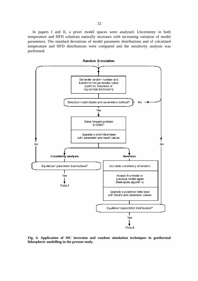
esent study, the random simulation and MC inversion were applied toic thermal models following the schematic algorithm in fig. 4. At first theandom numbers were generated using a pseudeo-random number generatoral. 1990). The random numbers were transformed into geothermal parametereach model at a time. Geometrically, the model was divided into domains thes of which were kept stationary during the simulations. The generation of eachalue was made independently according to the assumed distributions. Newere not dependent on the previous ones, but the random steps were takenusly and independently in all model blocks. The forward problem was solved

e difference code SHEMAT (Clauser & Villinger 1990) and the used models and results were collected to a data base. The data base includes all parameterall layers in one-dimensional models and all parameter values of all blocks insional models as well as the corresponding boundary conditions. Values of

ameters and solutions were not in discrete form (divided into classes) until theon of the distribution histograms.alization of the simulation algorithm was made in a rather pragmatic andward way. The first major aim was the uncertainty analysis of typicalic modelling. A new model was always generated from the very beginningriori model space, thus guaranteeing the prerequisite connection between they of model parameters and the uncertainty of results as well as statisticalnce were guaranteed. A modified simple random walk increases computationalmodel generation. The second major aim was inversion where the coolingwas rejected. An approved inversion result was reached by accepting proper

a posteriori model space in the first simulation process. The used thermal stateds to the uncertainty of the measured surface HFD data. Due to the inherent of the geothermal inversion problem, the simulated annealing was ineffectiveistic surface HFD value was used. In this process, it is not possible to find ael, but only to map the relative probabilities of the different alternatives (see

gaard & Tarantola (1995), for their discussion on the similar problem).

In paptemperatuparametertemperatuperformed

Fig. 4. Aplithospheri

32

ers I and II, a priori model spaces were analysed. Uncertainty in bothre and HFD solutions naturally increases with increasing variation of models. The standard deviations of model parameter distributions and of calculatedre and HFD distributions were compared and the sensitivity analysis was.

plication of MC inversion and random simulation techniques in geothermal

c modelling in the present study.

Unlikenormally conductivof the conparameterthermal co

When conditionsthe variatselected ‘simulation

In papaccordingresult is tparameterinverted te

In pape& Peltonedimensionusing the models wbetween tspace wasprocess, tcriterion. forward casurface HF

33

other normally deviated distributions, heat production was assumed to be log-distributed. In paper I, variation of the most important parameters (thermality and heat production rate, basal boundary conditions, temperature, and HFD)ductive lithospheric geothermal model have been studied. In paper II also others (temperature dependence of thermal conductivity and pressure dependence ofnductivity) were studied.random variation was directed only to rock properties selected boundary were fixed as constant values. Respectively, rock properties were fixed, whenion was directed to the basal boundary condition only. In combined cases,constant’ basal boundary conditions and parameter values were varied in thes, and other basal boundary values were kept constant.ers III and IV the samples of the a posteriori model spaces were formed to the acceptance rules of the Metropolis algorithm. The reached inversionhe a posteriori model space, consisting of equilibrated distributions of models. Uncertainties of the inversion results are given as standard deviations ofmperature and HFD distributions.r IV xenolith-derived temperature data at the mean depth of 208 km (Kukkonenn 1999) was added independently to the inverse simulation of the two-al Baltic-SKJ model. Firstly, the inversion was done following the fig. 4 andsurface HFD data as the fitting object. Secondly, the obtained a posterioriere mixed into a random order at the same time retaining the connectionhe parameters of each model and its results. The existing a posteriori model then utilized as a new a priori model space. In the new Metropolis samplinghe xenolith-derived temperature (with uncertainty) was used as the acceptingThis second process was performed without new model generation or newlculations. The final a posteriori model space is therefore in agreement with theD data and xenolith-derived temperatures in the mantle.

The four pused thermstep by stforward mimportant studied (sanalysis othermal codecreasedcalculatedand the mmodel oftemperatu

Jokinen J forward si(eds.) Thesymposiumthe worksthe 29th Gthe Earth’306 (3-4):

Randomgeothermaestimatingbasal temp

5. Publications

ublications presented in the appendix form an entity where the accuracy of theal models and the application of the MC method in this problem are improved

ep. In the first publication, the MC method used to calculate the accuracy ofodels is presented. In addition to uncertainty analysis, the effects of each mostmodel parameter on the accuracy of the results of the thermal models were

ensitivity analysis). The second work concentrates on accuracy and sensitivityf the modelling results on the temperature and pressure dependencies of thenductivity of rocks. In the third paper, the uncertainty of the thermal model is

by applying Metropolis sampling, thus setting acceptance conditions for surface HFD variation. The used inversion method improves both the resultsodel parameter distributions. In the fourth publication, the two-dimensional

the Baltic-SKJ transect is improved by entering xenolith-derived mantlere data into the inversion.

5.1. Paper I

& Kukkonen IT (1999a) Random modelling of the lithospheric thermal regime:mulations applied in uncertainty analysis. In: Clauser C, Lewis T & Rybach Lrmal regimes in the continental and oceanic lithosphere: selected papers of the

“Heat flow, seismic structure and seismicity in active tectonic regimes” andhop “Thermal regimes in the continental and oceanic lithosphere”, held duringeneral Assembly of the International Association of Seismology and Physics of

s Interior (IASPEI), Thessaloniki, Greece, August 18–28, 1997. Tectonophysics 277–292.

modelling technique was applied in uncertainty analysis of forwardl modelling of the lithospheric thermal regime. Results are presented for the effects of uncertainties in thermal conductivity, heat production rate, modelerature, and basal heat flow density on calculated lithospheric temperature and

HFD. Twoshield conhistory fro

Thermadistributedboundary based on standard deither in thA (A in µsame valu10 mW m

If conduncertainttemperatucalculateduncertaint(using temboundary

Kukkonenthermal trmodels aFennoscan

Measurand pressmetamorpFennoscanwas recordphonon coPressure crystalline

The temliterature conductivrepresentapredetermlithosphersuggest thto variatiocomparisoconductiv

35

models were analysed, first a 4-layer synthetic model representative of typicalditions with thick crust and lithosphere, and secondly a 2-dimensional casem the Fennoscandian (Baltic) Shield.l conductivity (normally distributed) and heat production (log-normally) as well as temperature or HFD (normally distributed, used as the lowercondition in the mantle) were randomly varied in the simulation. Calculations1500 independent cases of the layered model indicate, for instance, that aeviation (STD) of 50 K in calculated Moho temperature results in uncertaintiesermal conductivity of about 0.5 W m-1 K-1, in heat production rate of 0.2 log10

W m-3), 115 K in basal temperature or 1.7 mW m-2 in basal HFD. Again, thees result in the uncertainty of about 2 mW m-2 in calculated Moho HFD and-2 in calculated surface HFD.uctivity and heat production rate are varied simultaneously, the resulting

y in calculated Moho temperature increases to about 70 K. Adding also basalre variation increases the Moho temperature variation to about 85 K. Results using the 2-dimensional Baltic Shield transect indicate analogously thaty of temperature at the depth of 50 km (approximately at the Moho) is 35–60 Kperature as the lower boundary condition) and 50–85 K (using HFD as lower

condition). The corresponding variations in surface HFD are 6–15 mW m-2.

5.2. Paper II

IT, Jokinen J & Seipold U (1999) Temperature and pressure dependencies ofansport properties of rocks: Implications for uncertainties in thermal lithospherend new laboratory measurements of high-grade rocks in the Centraldian Shield. Surveys in Geophysics 20: 33–59.ements on thermal conductivity and on diffusivity as functions of temperatureure are presented for Archaean and Proterozoic mafic high-grade rockshosed in middle and lower crustal pressures, and situated in the centraldian Shield. Decrease of 12–20 % in conductivity and 40–55 % in diffusivityed between room temperature and 1150 K, which may be considered typical ofnductivity. Radiative heat transfer effects were not detected in these samples.

dependencies (up to 1000 MPa) of the samples are weak if compared to rocks in general, but relatively typical of mafic rocks.perature and pressure dependencies of thermal transport properties (data from

and the present study) were applied in an uncertainty analysis of lithospherice thermal modellings with random (MC) simulations using a 4-layer modeltive of the shield lithosphere. Model parameters were varied according toined probability functions and standard deviations were calculated foric temperature and HFD after 1500 independent simulations. The resultsat the variations (uncertainties) in calculated temperature and HFD values duens in the temperature and pressure dependencies of conductivity are minor inn to the effect produced by typical variations in the room temperature value of

ity, heat production rate or lower boundary condition values.

Jokinen J using the regimes in“Heat flow“Thermal General AEarth’s In306 (3-4):

The Mconductivprobabilitymodels. Cmodificaticarried ouas a fittingwith threemodel in Feither (1) the resultsuggestedand HFD,

The resrelatively ambiguityMC inverdistributioand narroDeteriorat

Jokinen Jthermal reJournal of

MC insimulationthermal rekimberlitetemperatuleast 240 thermal coas the low

36

5.3. Paper III

& Kukkonen IT (1999b) Inverse simulation of the lithospheric thermal regimeMonte Carlo method. In: Clauser C, Lewis T & Rybach L (eds.) Thermal the continental and oceanic lithosphere: selected papers of the symposium, seismic structure and seismicity in active tectonic regimes” and the workshopregimes in the continental and oceanic lithosphere”, held during the 29thssembly of the International Association of Seismology and Physics of theterior (IASPEI), Thessaloniki, Greece, August 18–28, 1997. Tectonophysics 293–310.C inversion method was applied to geothermal lithospheric models of

e heat transfer in steady-state conditions. A priori models were generated from distributions assigned to thermal conductivity and heat production rate of the

orresponding temperature and HFD values were calculated numerically, and theon of the a priori distributions into samples of the a posteriori distributions wast using the Metropolis algorithm as the acceptance rule and surface HFD values object. Two models were analysed, first a 1-dimensional layered earth model

crustal and one upper mantle layer, and secondly, a 2-dimensional lithosphericennoscandian Shield. The thermal conductivity and heat production rate were

evenly or (2) normally and log-normally distributed in the models. In both casess were generally similar in the sense that the same kinds of changes were by the inversion algorithm for conductivity, heat production rate, temperature, although the changes were not identical in details.ult indicates that the inversion tool is robust and able to reach solutions fromloosely constrained a priori parameter estimates. However, the general

of the geothermal inversion problem influences the results considerably. Thesion can be used for analysing the problem with the aid of the a posteriorins of different parameters. Improvement of results, i.e. shifting of mean valueswing of distributions were observed in many domains of the models.ion of the parameter estimates was not recorded.

5.4. Paper IV

& Kukkonen IT (2000) Inverse Monte Carlo simulation of the lithosphericgime in the Fennoscandian Shield using xenolith-derived mantle temperatures. Geodynamics 29: 71 – 85.version was applied in 2-dimensional conductive steady-state thermal of a 600 km long lithosphere transect in the Fennoscandian Shield. Thegime in the mantle was constrained with thermobarometric data derived from-hosted mantle xenoliths in eastern Finland, which suggest an averagere of 1250 ± 50 °C (1523 ± 50 K) at 208 km, but no partial melting down to atkm. A priori models were generated from probability distributions assigned to

nductivity and heat production rate values, as well as to the mantle HFD useder boundary condition in the simulations. The forward problem was solved with

the finite posteriori inversion,re-samplintemperaturesolutioncan be seeobtained rarea of FemW m-2 ino partial 250 km. Tthe transeThis transmelting. Tprovince atransports

37

difference code, and the modifications of the a priori distributions into adistributions were carried out using the Metropolis algorithm. The two-stage firstly using the measured surface HFD values as a fitting object, and secondly,g the obtained a posteriori models but using xenolith-derived mantle

re data as a fitting object, results in a considerable improvement in the and average values of temperature and HFD in the model. The improvementsn in the model results to a distance of about 400 km from the xenolith area. Theesults support a scheme that the mantle HFD is low in the thickest lithospherennoscandian Shield and about 10 ± 1 mW m-2 at about 200 km, and 13 ± 1n the uppermost subcrustal mantle. The inversion results suggest, that there ismelt-bearing asthenosphere under the transect at depths shallower than at leasthe seismic lithosphere-asthenosphere boundary is at depths of 110–170 km on

ct and corresponds to a temperature of about 1100 °C (1373 K) in the model.ition can be related to a zone of rheological weakening but not to the onset ofhe mantle temperature and HFD value in the Eastern Finland kimberlitere in agreement with models where small-scale convection (solid state creep)

heat to the base of the lithosphere at the depth of about 250 km.

The majoanalysis ofunction conditions

The reshields oncontinentapresent mdifferent u

The untypical va60–90 K, value can measured temperatu

In addithe use oftomographtemperatu1990). Rework whegeosciencZeyen 199Shield hav1999).

The mlower bouand tempegeneral le

6. Discussion and conclusions

r achievements of the present dissertation are the following: (1) uncertaintyf typical lithospheric thermal models, (2) assessment of the uncertainties ofof the individual uncertainties of input thermal parameters and boundary, and (3) application of MC inversion methods in geothermal modelling.sults of the uncertainty analysis can be generalized to apply to Precambrian a large scale. With caution, they can also be used for the Phanerozoic stabilizedl crust where the crustal and lithosphere thicknesses are comparable to theodels. And certainly, the qualitative conclusions on the relative importance ofncertainties of simulation results are valid in other continental areas as well.certainty analysis and inversions suggest that e.g. the Moho temperature (ariable presented in geothermal maps) can be obtained with an uncertainty at c.when the modelling is based on using surface HFD data as a fitting object. Thisbe decreased if there are other data on deep temperatures, independent of theHFD values, as was shown by the 2-D inversion utilizing xenolith-

res.tion to utilizing xenolith-temperatures another method may be provided e.g. by data on the temperature dependence of seismic P-wave velocity obtained fromic inversion studies on upper mantle (Furlong et al. 1995) or possibly by the

re dependence of conductivity in mantle in magnetotelluric studies (Korjaciprocally, geothermal models with uncertainty analyses complete researchre model parameters are temperature dependent. Facilities to combine differentes have been improved during frame projects such as the EUROPROBE (Gee &6) and SVEKALAPKO (Hjelt 1997) projects. Results from the Fennoscandiane recently been published within the GGT / SVEKA project (Korsman et al.

ost important parameters contributing to total modelling uncertainty are thendary condition, thermal conductivity, and the heat production rate. Pressurerature dependencies of thermal conductivity are less important as long as the

vels of thermal conductivity are correctly chosen in the model.

Generato thermaltemperatulaboratorydepth valuabout 34 kof knowlecould be pressure aconductivdecrease pressure-i100 km. T

MC inimprovingthem. Howmeasured indicated simulationsuch resul

This imdownwardsolidus cutemperatutemperatuthermal liSurely it geotherm and lithosmapped as

The prstationarymodels anincluded eand to acmajor comShield areRadiogeni1989a,b, 1so far, no important conductivextensiveldensity anPeltoniem

39

lly, any model is only as reliable as its input data, and this applies particularly properties and their pressure and temperature dependencies. In the lithosphere,re and pressure may range up to about 1800 K and 7000 MPa, respectively. The measurements of thermal conductivity in this study correspond to a maximume of about 100 km for temperature dependent measurements (up to 1150 K) andm for pressure dependent measurements (up to 1000 MPa). There is still lack

dge, comprehensive data sets on lower crustal and upper mantle materials thatused in simulated in situ conditions involving simultaneous control of bothnd temperature. Extrapolation of the linear pressure dependence of thermal

ity to pressures prevailing in the lower lithosphere suggests that the thermalof phonon conductivity may be partly or completely compensated by thenduced increase in the conductivity of upper mantle rocks at depths exceedinghe problem is further complicated by the radiative heat transfer effects.version was noted to be a practical tool in geothermal modelling, capable of the models, i.e. of shifting the mode values of distributions and narrowingever, the inherent ambiguity of thermal models cannot be avoided, even if the

data were perfect. The demonstration of non-uniqueness (Fig. 4 in paper III)that it is relatively easy to find an acceptable model using typical forward (try-and-error estimation of model parameters) but the representativeness ofts is much more difficult to judge.plies that thermal lithosphere thickness estimation in shields, based on the

continuation of a geotherm (temperature-depth curve) until it intersects arve or a mantle adiabat, may include considerable uncertainties. If the

re gradient in the mantle is of the order of 4–5 K km-1 and the uncertainty ofre calculation may exceed 200 K at the depth of 150 km (Fig. 8 in paper III), thethosphere thickness estimate is obtained with an uncertainty of about 50 km.is not surprising that mantle melting curves (Pollack & Chapman 1977) andfamilies (Pollack et al. 1993), which are generally used as tools in continentalpheric studies, have uncertainties. However, now these uncertainties have been well.

esent applications of random modelling and MC inversion were realized in a way, i.e. the boundaries between individual domains were kept constant in alld spatial autocorrelation of thermal conductivity or heat production rate was notither. It would be possible to modify the model generation scheme accordingly,complish it using e.g. the continuum approach (Niemi 1994). However, theplication is the lack of real autocorrelation data. The data on the Fennoscandian too sparse for a reasonable variogram analysis of thermal conductivity.c heat production has been surveyed extensively in Finland (Kukkonen993, Jõeleht & Kukkonen 1998) using either glacial till or outcrop samples, butvariogram study has been presented. However, the autocorrelation analysis is anaspect which should be developed further in future studies. As for thermal

ity, some associated information could be obtained from other studies ony surveyed petrophysical properties of rocks. However, the correlation betweend thermal conductivity was generally poor in the Finnish data set (Kukkonen &

i 1998).

Calculaconcludedcannot bepropertiesrandom simodels. Tthick contimproved.

40

ted uncertainties do not weaken previous geothermal models. It has been that thermal parameters vary in the earth and average values of model units defined accurately for the subsurface. The normal variation of the physical of geological and lithological units causes uncertainty in the models. Themulation method is proved to be a practical tool for improving geothermalhis work clearly demonstrates how accurate geothermal investigations into theinental crust have been carried out effectively and also how these can be still

AbramowitNew Yo

Balling NPShield i

Balling NPnorthern

Bear J & Vtranspor

Binder K &topics. I

BuntebarthCarslaw HS

ermák Vmillenn

ermák VHandboDordrec

ermák V Angenhand TecProperti

Clauser C (StegenaPublishe

Clauser C Handbo

Clauser C &basin, d

Dahl-JensePast tem

Deutsch CVedition.

Furlong KPconstrai

7. References

z M & Stegun IA (1972) Handbook of mathematical functions. Dover Publications, Inc.,rk. (1976) Geothermal models of the crust and uppermost mantle of the Fennoskandiann South Norway and the Danish embayment. J Geophys 42: 237–256. (1995) Heat flow and thermal structure of the lithosphere across the Baltic Shield and Tornquist Zone. Tectonophysics 244: 13–50.erruijt A (1987) Modeling groundwater flow and pollution (Theory and applications oft in porous media). D. Reidel Publishing Company, Dordrecht, Holland. Stauffer D (1984) A simple introduction to Monte Carlo simulation and some specializedn: Binder K (ed), Applications of the Monte Carlo Method, Springer Verlag: 1–36. G (1984) Geothermics, An introduction. Springler-Verlag, Berlin, 66 figures, 125 pp. & Jaeger IC (1959) Conduction of heat in solids, 2nd ed Oxford Univ. Press., London. (1971) Underground temperature and inferred climatic temperature of the pastium. Paleogeography, Paleoclimatol, Paleoecol 10, 1–19. & Haenel R (1988) Geothermal maps. In: Haenel R, Rybach L & Stegena L (eds)ok of terrestrial heat-flow density determination. Kluwer Academic Publishers,ht.& Rybach L (1982) Thermal conductivity and specific heat of minerals and rocks. In:eister G (ed), Landolt-Börstein: Numerical Data and Functional Relationships in Sciencehnology, New Series, Group V (Geophysical and Space Research), Vol. 1a (Physicales of Rocks). Springer, Berlin, p. 305–343.1988) Opacity – the concept of radiative thermal conductivity. In: Haenel R, Rybach L & L (eds) Handbook of terrestrial heat-flow density determination. Kluwer Academicrs, Dordrecht.& Huenges E (1993) Thermal conductivity of rocks and minerals. In: Clark SP (ed)ok of physical constants, The Geological Society of America, New York. Villinger H (1990) Analysis of conductive and convective heat transfer in a sedimentary

emostrated in Rheingraben. Geophys J Int 100: 381–414.n D, Mosegaard K, Gundestrup N, Clow GD, Johnsen SJ, Hansen AW & Balling N (1998)peratures directly from the Greenland ice sheet. Science 282: 268–271. & Journel AG (1998) GSLIB, Geostatistical software library and user’s guide, Second

Oxford University Press, New York, 345 pp.

, Spakman W & Wortel R (1995) Thermal structure of the continental lithosphere:

nts from seismic tomography. Tectonophysics 244: 107–117.

Gee DG & Contine

Geman S &images.

Greene JWComput

Haenel R, Determi

Hanley EJ,the temp

Heier KS &Geochim

Hjelt S-E (Finland

Ingber L (1Jokinen J (

tiheydenJõeleht A &

hydrogeJõeleht A &

basemen- IV. Te

Kaikkonensimulate

Kennett BL413–425

Kirkpatrick(4598):

Kolditz O &rocks: a

Korja T (Fennosc

Korsman KSVEKASvecofe

Kukkonen Baltic S

Kukkonen Baltic S

Kukkonen Survey

Kukkonen on geocstructur

Kukkonen geotherm(eds) HeGeophyCopenh

42

Zeyen HJ (1996) EUROPROBE 1996 – Lithosphere Dynamics: Origin and Evolution ofnts. Published by the EUROPROBE Secretariate, Uppsala University, 138 pp. Geman D (1984) Stochastic relaxation, Gibbs’ distribution and Bayesian restoration of

IEEE Trans., PAMI-6, 721–741. & Supowit KJ (1986) Simulated Annealing Without Rejected Moves. IEEE Trans, Oner-Aided Design. Vol. CAD-5, 1: 221–228.Rybach L & Stegena L (eds) (1988) Handbook of Terrestrial Heat-Flow Densitynation. Kluwer Academic Publishers, Dordrecht. Dewitt DP & Roy RF (1978) The thermal diffusivity of eight well characterized rocks forerature range 300–1000 K. Engineering Geology 12: 31–47. Adams JAS (1965) Concentration of radioactive elements in deep crustal material. Cosmochim Acta 29: 53–61.

1997) SVEKALAPKO, An EUROPROBE project, Abstracts of 2nd Workshop, Lammi,, 27. – 30.11.1997. University of Oulu, Department of Geophysics, Report no. 21.989) Very fast simulated re-annealing. Math. Comput. Modelling 12: 967–973.1997) Päätelmiä Keski-Suomen granitoidialueen rakenteesta painovoimakentän ja kivien mittauksiin perustuen. Tapio Tuomi (ed) XVIII Geofysiikan päivät 13.–14.5.1997. Kukkonen IT (1996) Heat flow density in Estonia – Assessment of Paleoclimatic and

ological effects. Geophysica 32 (3): 291–317. Kukkonen IT (1998) Thermal properties of granulite facies rocks in the Precambriant of Finland and Estonia. In: ermák V (ed) Heat flow and the structure of the lithosphere

ctonophysics 291 (1–4): 195–203. P & Sharma SP (1998) 2-D nonlinear joint inversion of VLF and VLF-R data usingd annealing. Journal of Applied Geophysics 39: 155–176.N & Nolet G (1978) Resolution analysis for discrete systems. Geophys R aste. Soc. 53:. S, Gelatt CD & Vecchi MP (1983) Optimization by Simulated Annealing. Science 220671–680. Clauser C (1998) Numerical simulation of flow and heat transfer in fractured crystalline

pplication to the hot dry rock site in rosemanowes (U.K.). Geothermics 27 (1): 1–23.1990) Electrical conductivity of the lithosphere, Magnetotelluric studies in theandian Shield, Finland. Ph.D. Thesis, Univ. Oulu, 179 pp., Korja T, Pajunen M, Virransalo P & GGT/SVEKA Working Group (1999) The GGT/ transect: structure and evolution of the continental crust in the Paleoproterozoicnnian orogen in Finland. International Geology Review 41: 287–333.IT (1988) Terrestrial heat flow and groundwater circulation in the bedrock in the centralhield. Tectonophysics 156 (1–2): 59–74.IT (1989a) Terrestrial heat flow and radiogenic heat production in Finland, the centralhield. Tectonophysics 164 (2–4): 219–230.IT (1989b) Terrestrial heat flow in Finland, the central Fennoscandian Shield. Geologicalof Finland. Nuclear waste disposal research, Report YST–68, 169 pp.IT (1993) Heat flow map of northern and central parts of the Fennoscandian Shield basedhemical surveys of heat producing elements. In: ermák V (ed) Heat flow and the

e of the lithosphere. Tectonophysics 225 (1–2): 3–13.IT (1995) Thermal aspects of groundwater circulation in bedrock and its effect on crustal

al modelling in Finland, the central Fennoscandian Shield. In: Balling N & Decker ERat flow and thermal regimes of continental lithosphere: papers presented at the Europeansical Society, XV General Assembly, Heat Flow and Lithospheric Thermal Regimes,

agen, 23–27 April 1990. Tectonophysics 244 (1–3): 119–136.

Kukkonen for adve

Kukkonen Karelia,structur

Kukkonen and its s

Kukkonen Shield:

Kukkonen properti

Laine E (1precambGeology

Lamontagndistribu

Lehmann Htransfer

MetropolisMetropolis

calculatMosegaard

GeophyNiemi A (1

approacPeltoniemi

Mining Peterson C

ComplePollack HN

lithosphPollack HN

data setPress F (19Press WH,

science Rebbi C (1

the MonRoyer JJ &

boundar239–255

Rybach L (HandboDordrec

Schatz JF Geophy

Seipold U 20: 145

Seipold U general

43

IT & Clauser C (1994) Simulation of heat transfer at the Kola deep-hole site: implicationsction, heat refraction and palaeoclimatic effects. Geophys J Int 116 (2): 409–420.IT, Gosnold WD & Šafanda J (1998) Anomalously low heat flow density in eastern Baltic Shield: a possible palaeoclimatic signature. In: ermák V (ed) Heat flow and thee of the lithosphere – IV. Tectonophysics 291 (1–4): 235–249.IT & Jõeleht A (1996) Geothermal modelling of the lithosphere in the central Baltic Shieldouthern slope. Tectonophysics 255 (1–2): 25–45.IT & Peltonen P (1999) Xenolith-controlled geotherm for the central Fennoscandianimplications for lithosphere-asthenosphere relations. Tectonophysics 304 (4): 301–315.IT & Peltoniemi S (1998) Relationships between thermal and other petrophysicales of rocks in Finland. Physics and Chemistry of the Earth 23 (3): 341–349.998) Geostatistical, geological and geophysical modelling of subsurface structures ofrian bedrock in Finland. Helsinki University of Technology, Laboratory of Engineering and Geophysics, Espoo.e M & Ranalli G (1996) Thermal and rheological constrains on the earthquake depthtion in the Charlevoix, Canada, intraplate seismic zone. Tectonophysics 257: 55–69., Wang K & Clauser C (1998) Parameter identification and uncertainity analysis for heat

at the KTB drill site using a 2-D inverse method. Tectonophysics 291: 179–194. N & Ulam S (1949) The Monte Carlo method. J Am Stat Assoc 44: 335–341. N, Rosenbluth AW, Rosenbluth MN, Teller AH & Teller E (1953) Equation of stateions by fast computing machines. J Chem Phys 21: 1087–1092. K & Tarantola A (1995) Monte Carlo sampling of solutions to inverse problems. Js Res 100: 12431–12447.994) Modeling flow in fractured medium. Uncertainty analysis with stochastic continuumh. Espoo 1994, Technical Research Centre of Finland, VTT Publications 184, 188 pp.S & Kukkonen IT (1997) Thermal properties of rocks in Finland. Finnish Association ofand Metallurgical Engineers, Publication Series A, N:o 106. Espoo. & Anderson JR (1987) A mean field theory learning algorithm for neural networks.x Systems 1: 995–1019. & Chapman DS (1977) On the regional variation of heat flow, geotherms, and

eric thickness. Tectonophysics 38: 279–296., Hurter SJ & Johnson JR (1993) Heat flow from the Earth’s interior: analysis of the global

. Rev. Geophys. 31 (3): 267–280.68) Earth models obtained by Monte Carlo inversion. J Geophys Res 73 (16): 5223–5234.Flannery BP, Teukolsky SA & Vetterling WT (1990) Numerical recipes in C, The art ofcomputing. Cambridge University Press, Cambridge.984) Monte Carlo calculations in lattice gauge theories. In: Binder K (ed) Applications ofte Carlo Method. Springer Verlag, 277–298. Danis M (1988) Steady state geothermal model of the crust and the problem of they conditions: application to a rift system, the southern Rhinegraben. Tectonophysics 156:.

1988) Determination of heat production rate. In: Haenel R, Rybach L & Stegena L (eds)ok of terrestrial heat-flow density determination. Kluwer Academic Publishers,ht.& Simmons G (1972) Thermal conductivity of earth materials at high temperature. Js Res 77 (35): 6966–6982.(1995) The variation of thermal transport properties in the Earth’s crust. J Geodynamics–154.

(1998) Temperature dependence of thermal transport properties of crystalline rocks – alaw. Tectonophysics 291: 161–171.

Sen M & Amsterd

Sharma SPsimulate

Smith L & 88:1: 59

Szu H & HTarantola A

ElsevierTurcotte D

problemWang K (1

problemWang K &

GeophyZoth G &

HandboDordrec

44

Stoffa PL (1995) Global optimization methods in geophysical inversion. Elsevier,am, 281 pp. & Kaikkonen P (1998) Two-dimensional non-linear inversion of VLF-R data usingd annealing. Geophys J Int 133: 649–668.Chapman DS (1983) On the thermal effects of groundwater flow. JGR, J Geophys Res B3–608.artley R (1987) Fast simulated annealing. Phys Lett A 122: 157–162. (1987) Inverse problem theory, Methods for data fitting and model parameter estimation., The Netherlands, 613 pp.L & Schubert G (1982) Geodynamics, Applications of continuum physics to geologicals. John Wiley & Sons, New York, 422 pp.989) An inverse finite element method for study of steady-state terrestrial heat flows. Ph.D. thesis, Univ. of Western Ontario, London, Canada. Beck AE (1989) An inverse approach to heat flow study in hydrologically active areas.s J Int 98: 69–84.Haenel R (1988) Thermal conductivity. In: Haenel R, Rybach L & Stegena L (eds)ok of terrestrial heat-flow density determination. Kluwer Academic Publishers,ht.