Uncertainties in Surface Colour Measurements

No. 95

Uncertainties in SurfaceColour Measurements

A NATIONAL MEASUREMENT

GOOD PRACTICE GUIDE

6304 GPG 95 11/5/06 10:32 am Page 1

The DTI drives our ambition of‘prosperity for all’ by working tocreate the best environment forbusiness success in the UK.We help people and companiesbecome more productive bypromoting enterprise, innovationand creativity.

We champion UK business at homeand abroad. We invest heavily inworld-class science and technology.We protect the rights of workingpeople and consumers. And westand up for fair and open marketsin the UK, Europe and the world.

This Guide was developed by the NationalPhysical Laboratory on behalf of the NMS.

6304 GPG 95 11/5/06 10:32 am Page 2

Measurement Good Practice Guide No.95

Uncertainties in surface colour measurements

J L Gardner

© Crown copyright 2006 Reproduced with the permission of the Controller of HMSO

and Queen's Printer for Scotland

ISSN 1368-6550

National Physical Laboratory Hampton Road, Teddington, Middlesex, TW11 0LW

Extracts from this report may be reproduced provided the source is acknowledged and the extract is not taken out of context.

Approved on behalf of the Managing Director, NPL

by Nigel Fox, Quality of Life Division

i

Contents Introduction..................................................................... 1

1.1 Measurement traceability.......................................................................................... 2 1.2 Surface colour measurement..................................................................................... 3

Measurement Uncertainty.................................................... 4

2.1 Propagation of uncertainty........................................................................................ 5 2.2 Propagation by component ....................................................................................... 7 2.3 Variance and covariance of the tristimulus values ................................................... 8

2.3.1 Random components ......................................................................................... 9 2.3.2 Systematic components ..................................................................................... 9 2.3.3 Sensitivity coefficients for colour quantities vs tristimulus values ................. 10

2.3.3.1 (x,y,Y) colour coordinates.................................................................................................. 11 2.3.3.2 (u,v,Y) colour coordinates.................................................................................................. 11 2.3.3.3 (u′,v′,Y) colour coordinates ................................................................................................ 12 2.3.3.4 (L*,a*,b*) colour coordinates ............................................................................................ 12 2.3.3.5 (L*,u*,v*) colour coordinates ............................................................................................ 13 2.3.3.6 (L*,C*,h) colour coordinates.............................................................................................. 14

Transfer measurement of reflectance ................................... 15

3.1 Uncertainty in the reference reflectance ................................................................. 17 3.2 Offsets in the transfer.............................................................................................. 19 3.3 Scaling of the transfer ............................................................................................. 19 3.4 Wavelength errors in the transfer............................................................................ 19

Uncertainty components for a typical spectrophotometer .......... 20 Example calculation ......................................................... 22 Conclusion..................................................................... 28 References .................................................................... 30

ii

List of Tables Table 1: Typical uncertainty specification for a white reference artefact (coverage factor of

k=1 assumed). ....................................................................................................... 17 Table 2: Description of the worksheets contained in the Surface Colour UC spreadsheet. 23 Table 3: Component uncertainty values used for the example calculations ....................... 25 Table 4:Values of the various colour quantities calculated for the coloured tiles .................. 25 Table 5: Uncertainties in the various colour quantities for the coloured tiles, propagated from

the uncertainty components described in the text ........................................................... 26 List of Figures Figure 1: Uncertainties in (u’,v’) chromaticity for the deep blue tile, by component as

identified in Table 3. Component 9 is the sum over all effects. .......................... 26 Figure 2: Uncertainties in (a*,b*) colour coordinates for the deep blue tile, by component as

identified in Table 3. Component 9 is the sum over all effects ........................... 27

Introduction

IN THIS CHAPTER

11

Measurement traceability

Surface colour measurement

Good Practice Guide 95 Chapter 1 2

1.1 Measurement traceability The term “traceability” applied to measurement can have different meaning to different people. In a narrow sense, it can be taken as a measurement referenced to some artefact that has been calibrated elsewhere. In a wider sense, it is taken to mean measurement with high integrity. This does not necessarily mean high accuracy, or high precision, but a measurement that includes an estimate of the uncertainty, or range of values about the specified value within which the measurement might lie with a reasonable probability. The user can then judge whether the result is fit-for-purpose, and can determine whether measurements made at different times, on different equipment, and/or by different operators are significantly different. The term is however formally defined by the International Organisation for Standardisation Vocabulary for International Metrology as:

property of a measurement result relating the result to a stated metrological reference through an unbroken chain of calibrations of a measuring system or comparisons, each contributing to the stated measurement uncertainty

NOTES 1. For this definition, a ‘stated metrological reference’ can be a definition of a

measurement unit through its practical realization, or a measurement procedure, or a measurement standard.

2. A prerequisite to metrological traceability is a previously established calibration hierarchy.

3. Specification of the stated metrological reference must include the time at which the stated metrological reference was used when establishing the calibration hierarchy.

4. The abbreviated term ‘traceability’ is sometimes used for “metrological traceability” as well as for other concepts, such as “sample traceability” or “document traceability” or “instrument traceability”, where the history (‘trace’) of an item is meant. Therefore, the full term should be preferred.

5. For measurements with more than one input quantity to the measurement function, each of the input quantities should itself be metrologically traceable.

Traceable measurement also involves the use of defined and verified procedures and archive of data, for both intermediate and final results, so that any subsequent questions about the integrity of the measurement can be answered. Modern traceability is also taken to mean that uncertainties are estimated in a consistent manner, as described in the ISO Guide to the Expression of Uncertainty in Measuremen. This document applies those principles to the field of surface colour measurement, where the colour quantities are calculated from measurements of spectral reflectance at a range of wavelengths through the visible part of the spectrum. It covers the measurement process itself – variations due to sample spatial-non-uniformity, angular effects and sample orientation are beyond the scope of this document. Understanding the uncertainties in the measurement process can in fact be used to determine whether sample variations are significant.

Chapter 1 Good Practice Guide 95 3

1.2 Surface colour measurement Colorimetric values for surfaces are usually calculated from measured values of reflectance vs wavelength determined with a double-beam spectrophotometer by comparison to a reference reflector. Results may be specified in a number of forms, all as triplets representing a 3-dimensional value; one of these values is usually an estimate of the luminance factor or lightness of the surface, and the remaining pair indicate the attribute usually taken as a chromaticity (or in the common jargon, ‘colour’ or ‘hue’). Physical measurement of colour is meant to mimic the response of the eye, by specifying three colour-matching functions representing the relative response of the trichromatic human vision system to light at different wavelengths. These agreed functions, specified by Commission Internationale Eclairage (CIE), allow measurements made in different laboratories to be directly compared. The convolution of the colour-matching functions with the spectral power distribution reaching the eye yields the three tristimulus values; various colour quantities are then calculated in terms of the tristimulus values. The spectral distribution of light reaching the eye is modified by reflection from a surface. A source of variability in surface colour measurement is then the spectral power distribution of the illumination system used for measurement. To remove this variability, surface colours are calculated from direct measurements of spectral reflectance with an assumed spectral power distribution of the source; common illuminant distributions are also specified by CIE. Any specification of surface colour should nominate the illuminant distribution and also the set of colour-matching functions used for its calculation, e.g. the CIE 1931 standard colorimetric observer (2° field-of-view) or the CIE 1964 standard colorimetric observer (10° field-of-view). In this Guide, we describe the methods to estimate the uncertainties in surface colour quantities derived from reflectance measurements, based on component uncertainties in both the measurement process and the reference reflectance values used to calibrate the spectrophotometer.

Measurement Uncertainty

IN THIS CHAPTER

22

Propagation of uncertainty

Propagation by component

Variance and covariance of the tristimulus values

» Random components

» Systematic components

» Sensitivity coefficients for colour quantities vs tristimulus values


2.1 Propagation of uncertainty Uncertainty propagation is described in detail in the ISO Guide to the Expression of Uncertainty in Measurement. The square of the uncertainty (the variance) in a quantity X formed by combining measured quantities xi through the relationship 1 2( , ,.. )NX f x x x= is given by

2 1

2 2

1 1 1( ) ( ) 2 ( , )

N N N

i i ji i j ii i j

f f fu X u x u x xx x x

−

= = = +

⎛ ⎞∂ ∂ ∂= +⎜ ⎟∂ ∂ ∂⎝ ⎠∑ ∑ ∑ , (1)

where ( )iu x is the uncertainty in ix and ( , )i ju x x is the covariance of ix and jx . This equation assumes that X depends linearly on the input values xi in a small range (the uncertainty) about their measured values. The derivatives if x∂ ∂ are sensitivity coefficients for the dependence of X on the various measured quantities, that is, they represent the rate of change of the output quantity X on the various input quantities xi. The uncertainty of those input values for which the rate of change of the output X is large contribute most strongly to the uncertainty in X. When we make a spectral measurement to determine colour, we are measuring similar quantities xi at different wavelengths. Various components of the measurement contribute to the uncertainties of the xi values. Some of those components vary at one wavelength in a manner totally independent of that at another wavelength. Commonly described as “noise”, these components are random or uncorrelated between wavelengths. The inter-dependence, or covariance, between values at different wavelengths is then zero and Eq. (1) reduces to

2

2 2

1( ) ( )

N

ii i

fu X u xx=

⎛ ⎞∂= ⎜ ⎟∂⎝ ⎠∑ , (2)

the “sum of squares” applied when the input quantities vary, or are assumed to vary, in a random manner. Other measurement uncertainties can arise from an underlying influence factor that affects the system of all measured values xi and are hence described as being systematic. As the factor varies within its uncertainty band, the measured values vary in a related, or correlated, manner. Many systematic effects have a single influence factor. This then leads to complete correlation between the values xi at different wavelengths for that component, for which their covariance is given by

( , ) ( ) ( )i j i ju x x u x u x= ± (3) For the case of all correlations being positive, Eq. (1) then reduces to

1

( ) ( )N

ii i

fu X u xx=

∂=

∂∑ (4)


for completely correlated data, but where the correlations can be positive or negative, Eq. (4) also applies provided we attach a sign to the uncertainty, as discussed below in Section 2.3.2. In the general case, the uncertainties of the input values contain a mixture of independent random and systematic components. When these are combined into total uncertainty for the value xi (by sum-of-squares, because the individual components are independent), the values at different wavelengths are partly correlated. It is often convenient to describe the general case in terms of the correlation coefficient r, defined by ( , ) ( ) ( )i j i ju x x ru x u x= (5) where r is zero for uncorrelated data and ranges in value from –1 to +1: for fully correlated data, 1r = . In terms of the correlation coefficient, Eq. (1) becomes

2 1

2 2

1 1 1( ) ( ) 2 ( , ) ( ) ( )

N N N

i i j i ji i j ii i j

f f fu X u x r x x u x u xx x x

−

= = = +

⎛ ⎞∂ ∂ ∂= +⎜ ⎟∂ ∂ ∂⎝ ⎠∑ ∑ ∑ (6)

If we form another quantity Y by combining the measured quantities xi through the relationship 1 2( , ,.. )NY g x x x= , the uncertainty in Y is given by an expression similar to that of Eq. (1), but now the quantities X and Y are correlated through dependence on the common set xi. In effect, the values xi become the common influence factors for the quantities X and Y. The covariance between X and Y is given by

1 1

( , ) ( , )N N

i ji j i j

f gu X Y u x xx x= =

∂ ∂=

∂ ∂∑∑ . (7)

The variance of a quantity is its covariance with itself, 2 ( ) ( , )i i iu x u x x≡ . Hence Eq. (1) is expressed in matrix form as 2 ( ) x x xu X = Tf U f , (8) where

1 2

..xn

f f fx x x

⎛ ⎞∂ ∂ ∂= ⎜ ⎟∂ ∂ ∂⎝ ⎠

f (9)

is a row vector of sensitivity coefficients ( x

Tf is its transpose) and ( )( , )x i ju x x=U (10) is the N X N variance-covariance matrix of squares-of-uncertainty (variance) in diagonal elements, covariance values elsewhere.


Similarly, the covariance between two combinations of the same data is given in matrix form ( , ) x x xu X Y = Tf U g , (11) where

1 2

..xn

g g gx x x

⎛ ⎞∂ ∂ ∂= ⎜ ⎟∂ ∂ ∂⎝ ⎠

g (12)

Where one set of input values X are combined to form a number of output quantities Y, these expressions are generalised further. The variance-covariance matrix of the output quantities Uy is propagated from that of the input quantities Ux as

y x= ΤU QU Q (13) where Q is a matrix of sensitivity coefficients for the output quantities (by row) in terms of each of the input quantities (by column). For colorimetric uncertainties, the sum forms of Eqs. (2) and (4) are convenient for propagating uncertainties of the spectral measurements to those of tristimulus values, and the matrix form of Eq. (13) is useful for propagating uncertainties from the tristimulus values to the required colour quantities. 2.2 Propagation by component The total variance of the value at one wavelength is the sum of the variances of the components. Similarly, the total covariance between pairs of spectral values is the sum of the covariances for all the components. Random components contribute only to the variance at a given point. The combination of random and systematic components means that the covariance between measured spectral values is no longer zero, as for purely random components, or complete, as for purely systematic components, but is partial; the resultant correlation coefficients have magnitudes greater than zero but less than one. These correlations must be taken into account by using Eq. (6) or its matrix equivalent, Eq. (8) to propagate the total uncertainty at different wavelengths through to the uncertainty of a result that combines the spectral values. However, each of the components contributing to the overall uncertainty of the spectral measurements xi can be treated independently and its contribution to the variance of the combined result X be calculated. Similarly, its contribution to the covariance between two combined results X and Y can be propagated. Then all the contributions to the variance and covariance are summed to find the totals over all components. Propagating by component of the spectral measurement itself has three advantages. The first is that the effect of individual components of the spectral measurement on the uncertainty of the final desired quantities is determined. These individual components arise from the spectral measurement procedure itself and understanding the uncertainty contributed to a final desired result can lead to improved procedures. The second is that individual


components are either random (uncorrelated) or systematic (fully correlated), and simple sums can be used to calculate the variance of a combination. This is particularly useful when the spectral values are measured at a large number of points. Thirdly, the covariance between combinations is a simple sum for random components (again useful when the number of spectral points is large) and a simple product for systematic components. The latter fact arises because the different combinations of fully-correlated values are themselves fully correlated. 2.3 Variance and covariance of the tristimulus values Tristimulus values X,Y,Z for surface colour measurements are calculated from spectral reflectance values as a convolution of the spectral reflectance R, an agreed illuminant spectral power distribution S, and the CIE colour matching functions , ,x y z . In integral form,

( ) ( ) ( )

( ) ( ) ( )

( ) ( ) ( )

X S x R d

Y S y R d

Z S z R d

λ λ λ λ

λ λ λ λ

λ λ λ λ

=

=

=

∫∫∫

(14)

The illuminant distributions are usually given in relative terms, normalized so that

( ) ( ) 100S y dλ λ λ =∫ . (15)

Then the tristimulus values are relative, with Y = 100 for a surface with R(λ) = 1 for all wavelengths. Note, however, that reflectance is often specified as a percentage, in the range 0% −100%. The colour-matching functions are specified over the wavelength range 360 nm to 830 nm; it is common to use a limited range from 360 nm to 780 nm. For reflectance data measured at N discrete wavelengths, the integrals are replaced by the sum forms,

1

1

1

N

i i i iiN

i i i ii

N

i i i ii

X S x R

Y S y R

Z S z R

=

=

=

= Δ

= Δ

= Δ

∑

∑

∑

(16)

where the i subscript is used to denote wavelength. The Δi term is included as a weight for the contribution of the ith term to the integral. For data recorded at equally spaced intervals λΔ , i λΔ = Δ is constant and can be taken outside the sum (this form applies because the

colour-matching functions are zero at their limits). For data recorded at a varying spacing, as is common with diode array spectrometers having a non-linear wavelength scale, Δi varies through the spectrum.


For trapezoidal integration,

1 2 1

1

1 1

( ) / 2( ) / 2

( ) / 2 1or N N N

i i i i N

λ λλ λλ λ

−

+ −

Δ = −Δ = −Δ = − ≠

(17)

The colour-matching functions for surface colours are usually those for a 10° field-of-view; the illuminant distribution depends on the application, but is typically CIE Standard Illuminant D65. The illuminant and colour-matching functions are tabulated distributions that carry no uncertainty. From Eqs. (16), the sensitivity coefficients for the dependence of the tristimulus values on the reflectance measurements are

i i ii

i i ii

i i ii

X S xRY S yRZ S zR

∂= Δ

∂

∂= Δ

∂∂

= Δ∂

(18)

Various effects which may be random or systematic between wavelengths contribute to the uncertainties of the reflectance measurements and hence of the tristimulus values, and to the covariance between the tristimulus values. Each of these effects is treated in turn, as the sole source of uncertainty, and the variances and covariances summed over all effects to form the total variance-covariance matrix of the tristimulus values. 2.3.1 Random components For uncorrelated uncertainty components of the reflectance, the variance of the X tristimulus value is given from Eq. (2) by

( )22 2

1

( ) ( )N

i i i ii

u X S x u R=

= Δ∑ , (19)

with similar expressions for Y and Z. The covariance between the X and Y values is given from Eq. (7) by

2 2 2

1

( , ) ( )N

i i i i ii

u X Y S x y u R=

= Δ∑ , (20)

again with similar expressions for the remaining pairs of tristimulus values. 2.3.2 Systematic components Systematic components are correlated between wavelengths. Most effects have a positive correlation between pairs of values at different wavelengths, but not all. For example, if the wavelength is in error by a systematic positive offset, reflectance values fall where the slope of the reflectance is negative and rise where the slope of the reflectance is positive; reflectance values at a pair of wavelengths where the reflectance values have opposite slopes


are then negatively correlated. For each component effect, we calculate the magnitude of the uncertainty in spectral reflectance as a product of the sensitivity coefficient for that effect, and the uncertainty of the effect. While uncertainties are usually taken as positive, correlations are correctly handled in the linear sum of Eq. (4) if they are treated as carrying the sign of the sensitivity coefficient4. If p is a parameter describing the effect in question, the signed uncertainty in reflectance is given by

( ) ( )is i

dRu R u pdp

= . (21)

The uncertainty in the X tristimulus value for this effect is then given by

1

( ) ( )N

s i i i s ii

u X S x u R=

= Δ∑ , (22)

where the result of this sum may be positive or negative. The variance, or square of the uncertainty, is of course positive. Similar expressions hold for the uncertainty of the Y and Z tristimulus values. Further, the covariance between pairs of tristimulus values is given by the product of the uncertainty sums, e.g.

( , ) ( ) ( )s su X Y u X u Y= . (23) The tristimulus values are fully correlated for fully correlated components of the spectral measurement, as are any of the colour values calculated from the tristimulus values. 2.3.3 Sensitivity coefficients for colour quantities vs tristimulus values While all the colorimetric quantities that may be required can ultimately be specified in terms of the measured spectral reflectance values themselves, and hence uncertainties propagated directly from those of the reflectance measurements, the expressions can become unwieldy. It is more convenient to calculate the tristimulus values and uncertainties (including correlations) and then propagate these to the final colour quantities. In some cases, this latter propagation can involve more than one stage. Below are sensitivity matrices for various colour quantities, in terms of the tristimulus values X, Y and Z. The variance-covariance matrix for the tristimulus values is formed as

2

2

2

( ) ( , ) ( , )( , ) ( ) ( , )( , ) ( , ) ( )

XYZ

u X u X Y u X Zu X Y u Y u Y Zu X Z u Y Z u Z

⎡ ⎤⎢ ⎥= ⎢ ⎥⎢ ⎥⎣ ⎦

U (24)

The variance-covariance matrix for a general colour triplet a,b,c is then given by

abc abc XYZ abc= ΤU Q U Q (25)


where the sensitivity matrix Q is of the form

abc

a a aX Y Zb b bX Y Zc c cX Y Z

∂ ∂ ∂⎡ ⎤⎢ ⎥∂ ∂ ∂⎢ ⎥∂ ∂ ∂⎢ ⎥= ⎢ ⎥∂ ∂ ∂

⎢ ⎥∂ ∂ ∂⎢ ⎥⎢ ⎥∂ ∂ ∂⎣ ⎦

Q (26)

2.3.3.1 (x,y,Y) colour coordinates The (x,y) chromaticity values are given simply as

xy

XxT

= , xy

YyT

= , with xyT X Y Z= + + . (27)

The sensitivity matrix is

2 2 2

2 2 2

0 1 0

xy xy xy

xyYxy xy xy

Y Z X XT T T

Y X Z YT T T

+ − −⎡ ⎤⎢ ⎥⎢ ⎥⎢ ⎥− + −

= ⎢ ⎥⎢ ⎥⎢ ⎥⎢ ⎥⎣ ⎦

Q (28)

Where the illuminant distribution is normalised according to Eq. (15) and reflectance is specified in the range 0 −1, the value of Y is in the range 0 −100. The linear dependence of the numerators of Eq. (27) for the x,y sensitivity coefficients on the tristimulus values has two important consequences. Any spectral uncertainty component that is a constant multiplied by the spectral value leads to zero uncertainty in the x and y chromaticity values (and also u, v, u′ and v′). This is true for an uncertainty in the relative value of the reference or in the transfer, as expected since the chromaticity values are ratios of the tristimulus values to their sum. 2.3.3.2 (u,v,Y) colour coordinates In a manner similar to the treatment for (x,y,Y) above:

4

uv

XuT

= , 6

uv

YvT

= with 15 3uvT X Y Z= + + (29)


The sensitivity matrix for the dependence of (u,v,Y) on the tristimulus values is

2 2 2

2 2 2

60 12 60 12

6 6 18 18

0 1 0

uv uv uv

uvYuv uv uv

Y Z X XT T T

Y X Z YT T T

+ − −⎡ ⎤⎢ ⎥⎢ ⎥

− + −⎢ ⎥= ⎢ ⎥⎢ ⎥⎢ ⎥⎢ ⎥⎣ ⎦

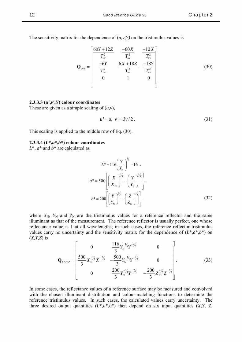
Q (30)

2.3.3.3 (u′,v′,Y) colour coordinates These are given as a simple scaling of (u,v),

' , ' 3 / 2u u v v= = . (31) This scaling is applied to the middle row of Eq. (30). 2.3.3.4 (L*,a*,b*) colour coordinates L*, a* and b* are calculated as

13

N

* 116 16YLY⎛ ⎞

= −⎜ ⎟⎝ ⎠

,

1 1

3 3

N N

* 500 X YaX Y

⎡ ⎤⎛ ⎞ ⎛ ⎞⎢ ⎥= −⎜ ⎟ ⎜ ⎟⎢ ⎥⎝ ⎠ ⎝ ⎠⎣ ⎦

,

1 1

3 3

N N

* 200 Y ZbY Z

⎡ ⎤⎛ ⎞ ⎛ ⎞⎢ ⎥= −⎜ ⎟ ⎜ ⎟⎢ ⎥⎝ ⎠ ⎝ ⎠⎣ ⎦

. (32)

where XN, YN and ZN are the tristimulus values for a reference reflector and the same illuminant as that of the measurement. The reference reflector is usually perfect, one whose reflectance value is 1 at all wavelengths; in such cases, the reference reflector tristimulus values carry no uncertainty and the sensitivity matrix for the dependence of (L*,a*,b*) on (X,Y,Z) is

1 23 3

N

1 2 1 23 3 3 3

* * * N N

1 2 1 23 3 3 3

N N

1160 03

500 500 03 3

200 20003 3

L a b

Y Y

X X Y Y

Y Y Z Z

− −

− −− −

− −− −

⎡ ⎤⎢ ⎥⎢ ⎥⎢ ⎥= −⎢ ⎥⎢ ⎥⎢ ⎥−⎢ ⎥⎣ ⎦

Q . (33)

In some cases, the reflectance values of a reference surface may be measured and convolved with the chosen illuminant distribution and colour-matching functions to determine the reference tristimulus values. In such cases, the calculated values carry uncertainty. The three desired output quantities (L*,a*,b*) then depend on six input quantities (X,Y, Z,


XN,YN,ZN) carrying uncertainty, and correlations. Hence, a more complex 3×6 sensitivity matrix and 6×6 variance-covariance matrix are required for the uncertainty propagation (not covered here). 2.3.3.5 (L*,u*,v*) colour coordinates These are defined as

1

3

N

* 116 16YLY⎛ ⎞

= −⎜ ⎟⎝ ⎠

, N* 13 *( ' ' )u L u u= − , N* 13 *( ' ' )v L v v= − (34)

where u′, v′ are CIE 1976 chromaticity coordinates of Eq. (31) and u′N, v′N are similar quantities for the illuminant alone. First we calculate the covariance matrix ' 'Lu vU for the quantities L*, u′ and v′, for which the sensitivity matrix in terms of the tristimulus values is

1 23 3

N

* ' ' 2 2 2

2 2 2

1160 03

60 12 60 12

9 9 27 27

L u vuv uv uv

uv uv uv

Y Y

Y Z X XT T T

Y X Z YT T T

− −⎡ ⎤⎢ ⎥⎢ ⎥⎢ ⎥+ − −

= ⎢ ⎥⎢ ⎥⎢ ⎥− + −⎢ ⎥⎣ ⎦

Q , (35)

where 15 3uvT X Y Z= + + . The covariance matrix * ' 'L u vU for the quantities L*, u′ and v′ is then * ' ' * ' ' * ' 'L u v L u v XYZ L u v= TU Q U Q (36) The sensitivity matrix for the quantities L*, u* and v* in terms of L*, u′ and v′ is

* * *' N

N

1 0 013( ' ') 13 * 013( ' ') 0 13 *

L u v u u Lv v L

⎡ ⎤⎢ ⎥= −⎢ ⎥⎢ ⎥−⎣ ⎦

Q , (37)

and the final uncertainties and correlations are carried in the variance-covariance matrix * * * * * * ' ' * * *L u v L u v Lu v L u v= TU Q U Q . (38)


2.3.3.6 (L*,C*,h) colour coordinates The quantities, chroma and hue angle are calculated from either (a*,b*) or (u*,v*) colour values. Taking the (a*,b*) example,

2 2* * *C a b= + , 1 *tan*

bha

− ⎛ ⎞= ⎜ ⎟⎝ ⎠

. (39)

We first calculate the variance-covariance matrix * * *L a bU for L*a*b* from that of the tristimulus values: * * * * * * * * *L a b L a b XYZ L a b= TU Q U Q . (40) The sensitivity matrix for the quantities L*, C* and h in terms of L*, a* and b* is

* *

2 2

1 0 0* *0* ** *0* *

L C ha bC Cb a

C C

⎡ ⎤⎢ ⎥⎢ ⎥⎢ ⎥=⎢ ⎥⎢ ⎥⎢ ⎥−⎣ ⎦

Q , (41)

and the final uncertainties and correlations are carried in the variance-covariance matrix * * * * * * * *L C h L C h La b L C h= TU Q U Q . (42) Hue angle is usually quoted in degrees. Values and uncertainties calculated above are in radians and must be scaled by 180/pi. Hue angle and chroma are also calculated from (u*,v*) chromaticities; uncertainties in these are found by substituting (u*,v*) for (a*,b*) in the above equations. Saturation s may be required in place of chroma; s=C*/L* and it is a simple matter to modify the sensitivity matrix * *L C hQ to accommodate this change.

Transfer measurement of reflectance

IN THIS CHAPTER

33

Uncertainty in the reference reflectance

Offsets in the transfer

Scaling of the transfer

Wavelength errors in the transfer


Spectral reflectance may be required for various geometric conditions. It is not generally measured from first principles but is measured against a reference standard. Hence, the spectral reflectance iR can be written as a transfer from that of a reference standard iR ,

i i iR t= R . (43) Uncertainties in the spectral value iR arise both from those of the reference value and those introduced by the spectral transfer. Colour values are formed by combining the spectral reflectance measurements at different wavelengths. Systematic effects in a spectral measurement have a cooperative relationship between wavelengths, that is, the values at different wavelengths are correlated. Correlations also exist between the reference values at different wavelengths, arising from systematic effects in the methods used to derive them. For uncertainty components of the reference spectrum, from Eq. (43) we have ( ) ( )i i iu R t u= R , (44) whereas for components in the transfer we have ( ) ( )i i iu R u t= R . (45) In both cases we calculate the transfer value as the ratio i i it R= R (46) This transfer ratio is measured directly in a double-beam spectrophotometer. In a single-beam instrument, it is calculated from separate measurements on the test and reference objects. A wide range of instruments and methods are used for spectral reflectance measurements, too diverse to be covered here. Part of the art of spectrophotometry is the identification of factors contributing to the uncertainty of the spectral measurements. This guide covers only the propagation of uncertainty from spectral reflectance to colour values. It is assumed that known systematic effects in the transfer are corrected. These include background offsets, scaling of the absolute value, and non-linearities, for example. Each correction has an uncertainty, which may be wavelength dependent, associated with it. Some factors, such as background offset, may be subtracted automatically as part of the measurement or instrument calibration process, but carry an uncertainty with both random (noise) and systematic (drift) components. For most measurements, contributing uncertainties fall into 4 types, each with components that are either random or systematic across wavelengths.


3.1 Uncertainty in the reference reflectance Reference reflectors used to calibrate the response of a spectrophotometer usually have high values of reflectance (for the chosen geometry) that are relatively constant across the wavelength spectrum. Systematic effects tend to dominate the uncertainty budget, particularly those that affect the absolute value of the reflectance, and the values at different wavelengths are highly correlated. Strictly, the supplier of the calibrated reference spectral data should provide the full variance-covariance uncertainty matrix of the data, and this be used to propagate the reference uncertainty components. Most often, these full data are not available. In most cases, however, the reference uncertainty is not a dominant component and its contribution to colour uncertainties can be estimated by simpler means.

Table 1: Typical uncertainty specification for a white reference artefact (coverage factor of k=1 assumed).

The ratio specified is that of systematic uncertainty to total uncertainty

Wavelength (nm)

0°:di Reflectance R

(%)

Total relative uncertainty

urel(R) (% of value)

Total relative systematic component

(% of value) Ratio

360 61.88 0.335 0.261 0.780

380 74.37 0.237 0.168 0.708

400 82.18 0.158 0.113 0.715

420 85.7 0.13 0.086 0.664

440 87.17 0.139 0.076 0.548

460 88.02 0.119 0.072 0.608

480 88.75 0.100 0.072 0.716

500 89.36 0.100 0.072 0.723

520 89.78 0.103 0.073 0.709

540 90.01 0.106 0.073 0.689

560 90.13 0.109 0.073 0.670

580 90.21 0.109 0.073 0.670

600 90.32 0.108 0.074 0.683

620 90.48 0.109 0.074 0.677

640 90.64 0.110 0.074 0.671

660 90.79 0.109 0.074 0.677

680 90.90 0.106 0.074 0.702

700 90.96 0.104 0.074 0.715

720 90.98 0.104 0.074 0.715

740 90.97 0.102 0.075 0.736

760 90.95 0.100 0.075 0.751


780 90.91 0.100 0.075 0.751

800 90.84 0.105 0.075 0.715

820 90.74 0.115 0.075 0.653 Table 1 shows a table of values and uncertainties that might be provided for the 0°:di reflectance of a white reference tile. At a very minimum, the total systematic uncertainty contribution to the uncertainty should be provided as well as the total uncertainty, at each wavelength. The ratio column of Table 1 is not usually provided with the calibration data, but must be calculated. We see that the ratio of systematic to total uncertainties is relatively constant across the spectrum, with an average value of 0.69. Negative correlations due to wavelength errors are negligible because reference artefacts have little wavelength-dependent structure. It follows that the correlation coefficient between wavelength pairs is also approximately constant, with a value of 0.692 = 0.48. If the correlation coefficient r is constant, we can treat the uncertainty in the reference spectral reflectance as consisting of a random component

( )( ) ' 1 ( ) /100i rel i iu r u= −R R R (47) and a systematic component ( ) ' ( ) /100i rel i iu r u=R R R (48) where we have used the fact that the uncertainties in Table 1 are given as relative values, as percentage of the reflectance value, in the usual way. The reflectance values themselves are given in units of percent – care must be taken in deciphering the value of relative uncertainty components in such a case. These two random and systematic components are then propagated to the elements of the variance-covariance matrix for the tristimulus values. In general, reference reflectance data will be provided on a wider wavelength step (e.g. 20 nm as in Table 1) between values than that required for a colour measurement and calculation, which is typically 5 nm. These reference data are then interpolated to the finer wavelength scale of the colour measurement. Interpolation introduces further correlations between the reference spectral reflectance values. One method to avoid these extra correlations is to calculate the reference contributions to the tristimulus variance-covariance matrix by interpolating the measured spectral reflectance of the sample to the wavelengths of the reference data, calculating the contributions of Eqs. (19), (20) and (22) using the reference data spacing5. A simpler alternative is to interpolate not only the reference spectral data but also their uncertainties to the wavelengths of the sample measurement and calculate the random and systematic components as above for the constant correlation coefficient. This process will correctly estimate the contributions of the systematic components, but underestimate the contributions of the random components; when propagating the random components of the reference uncertainties, the result should be scaled by the square-root of the ratio of the reference data spacing to the sample measurement data spacing to compensate for this effect. This simplification is an approximation – if the reference uncertainty components are dominant, the more complicated alternatives should be used.


3.2 Offsets in the transfer Part of the calibration procedure for reflectance measurement with a double-beam spectrophotometer is running a baseline spectrum, with the sample beam blocked. This baseline will contain random electronic noise and may drift – an effect, systematic across wavelengths - during a series of measurements. These are examples of offsets in the transfer. Scattered light may also be present in one of the measurement beams. The offsets may contain a wavelength dependence, for example, due to a change in amplifier gain or change in detector type, but be quantifiable directly for a set of given measurement conditions as direct uncertainty components of the transfer, ( )iu t , for which the uncertainty in spectral reflectance is given by Eq. (45). 3.3 Scaling of the transfer Other uncertainty components of the transfer are specified as proportional to the signal. Random source noise is one such component, as is the systematic effect of any masking of either the sample or reference beams. Linearity is another effect systematic across wavelengths. Again the uncertainty of these effects may vary with wavelength (or signal strength in the case of linearity), but they are quantified in terms of the relative transfer ratio. Hence from Eq. (45) we have ( ) ( ) ( )i i rel i i i rel iu R u t t R u t= =R (49) 3.4 Wavelength errors in the transfer From Eqs. (45) and (46), if the uncertainty in wavelength is ( )u λ ,

( ) ( )

( )

is i i

i

i i i

i

Ru R u

R R u

λλ

λλ λ

∂=

∂

⎛ ⎞∂ ∂= −⎜ ⎟∂ ∂⎝ ⎠

RR

RR

(50)

Note that here we have formed a signed uncertainty because wavelength offsets can lead to both positive and negative correlations between the spectral reflectance values at different wavelength pairs.

Uncertainty components for a typical spectrophotometer

44


Uncertainty components must be identified for the actual spectrometer settings, such as measurement times, number of scans averaged, wavelength step, etc., used to record the sample and reference spectra. Baseline (zero) measurements with the sample beam blocked are used to determine signal offset levels, once the spectrophotometer has reached stable conditions after its initial warm-up. Wavelength-to-wavelength variation is analysed to determine random offset noise from the baseline measurements. Repeated baseline measurements are analysed to determine the drift, or systematic offset, which may apply over a given measurement period. Similarly, repeat measurements of the reference reflector signals can be analysed for random noise and drift uncertainty components; these are usually determined as relative values. The random component for these latter measurements of course includes both amplifier noise and source noise (arising from fluctuations in the lamp drive current). Analyses of these baseline and reference components should include any data selection or smoothing which may be applied to the measured values. Wavelength uncertainties are typically analysed by recording transmission spectra of a glass doped with rare-earth compounds. The positions of the various absorption peaks are fitted to a function representing wavelength vs position in the spectrum (often assumed linear). The standard deviation of the fit can be taken as an estimate of the random wavelength uncertainty; the standard deviation of the mean is an estimate of the wavelength offset uncertainty. Note that if only a few peaks are used, a Student’s t multiplier should be applied to these uncertainties. Fine resolution may be used to determine the scanning function, but offsets must be estimated for the resolution used during a measurement, particularly if unilateral slits (those opening on one side only) are used in the spectrophotometer. Non-linearities are estimated either with a multiple-aperture technique, by measuring the transmittance of calibrated neutral density filters or by measuring the reflectance of calibrated grey tiles. If the departure from linearity is significant, the data must be corrected. The uncertainty is typically specified as a fraction of the spectral reflectance in the mid-region, and it is systematic over all wavelengths. In a sphere-based reflectance measurement, the sphere gain varies with the sample reflectance; this effect becomes part of the non-linearity measurement. Factors affecting the absolute value of the reflectance, such as alignment (due to beam shift on the detector), angular setting for a specified geometry, baffles affecting one beam and not the other, etc, can be grouped as a relative scaling uncertainty systematic over all wavelengths. Scattered light within the system may be wavelength dependent. It can be analysed by using filters. If significant, a correction should be applied. The uncertainty (which may be wavelength dependent) is treated as an offset systematic over all wavelengths. Measurements on the one sample may be repeated a number of times and the results averaged. Variation here may be related to sample uniformity or positioning effects. Repeated measurements will reduce the effect of random components in the measurement process, but not the systematic components. Repeat measurements are in fact correlated by the systematic components of the process.

Example calculation 55


An Excel spreadsheet, Surface Colour UC v5-1, was coded with the algorithms described above. The worksheets in this workbook are shown in Table 2.

Table 2: Description of the worksheets contained in the Surface Colour UC spreadsheet

Main Holds the spectrum, displays results Reference Holds the reference data and its interpolation

UCcomponents

Holds the uncertainty components and values, propagated to each measured spectral reflectance value. Also holds the contribution of each component to the X,Y,Z tristimulus uncertainties and to the covariance between them. Variance-covariance matrices of the tristimulus values are also formed for each uncertainty component.

CIE Holds the CIE colour-matching functions and illuminants, on a 1 nm grid.

SensCoeffs

Holds the sensitivity coefficients for the tristimulus values vs reflectance at each wavelength of the measured spectrum. These are a convolution of the illuminant and colour-matching function distributions.

SensMatrices

Holds the 3x3 matrices of the sensitivity coefficients of the colour values vs tristimulus values, the intermediate matrix products and the total variance-covariance matrices for the various colour triplets.

xyY components

u'v'Y components

L*a*b* components

L*C*h components

These sheets calculate the uncertainties in the colour values for each uncertainty component. Plots are given for the chromaticity pair, by uncertainty component.

The workbook contains macros used to interpolate the reference spectrum and its uncertainties, to set dynamic ranges and to copy the wavelengths of the spectral measurement to the various tables; all formulae used for calculations are contained within the cells of the spreadsheet itself, and copied by the macro from the first wavelength line in the various tables. In version 5, cubic spline interpolation is used for the reference data, coded in a macro. The spectral reflectance values are pasted into columns A and B of the Main sheet, beginning at row 3. Column A contains wavelength in nm (assumed integer and of constant spacing) and column B contains the spectral reflectance, corrected for all known effects, in the range 0-100%. The rows beneath the spectrum in columns A and B must have their contents cleared. If the wavelength range or spacing for the pasted spectrum is different from that used previously, clicking the command button for New Wavelength Range counts the


number of wavelengths and sets the wavelength values in various worksheets. In the process of setting the wavelength values, formulae in the first wavelength row in those sheets are copied to subsequent rows. Copying the formulae has important consequences for the UCcomponents worksheet (see below). The observer and illuminant distributions, usually 10º field-of-view and Illuminant D65, respectively, can be changed by clicking the command button in the options area. The UCcomponents worksheet contains values for uncertainty components that might be identified for a typical double-beam spectrophotometer. The resultant uncertainty at each wavelength is calculated and these values propagated to the elements of the tristimulus variance-covariance matrix, depending on whether the component is identified as systematic or random across the spectrum. In the default sheet, component uncertainty values are taken as applying independently of wavelength. However, if a component is known to vary across the spectrum (e.g. relative source noise is generally larger at shorter wavelengths), a wavelength-dependent functional representation can be coded in the first wavelength row, and scaled by the value parameter. Clicking the New Wavelength Range button in the Main sheet copies all the formulae from the first wavelength row to subsequent rows. Non-linearity can be defined in a number of ways, and have a number of causes. Incorrect offsets in an automated system lead to large errors near zero values; detector non-linearities due to saturation generally lead to reduced signal values at high signals. In a double-beam instrument with recorded 100% levels and zero baselines, non-linearities are likely to be compensated at those levels. Hence, the default non-linearity function assumes a specified relative uncertainty at the 50% reflectance level, tapering linearly to zero uncertainty at 0% reflectance and 100% reflectance. Component values in the default sheet are shown in Table 3. Note that to avoid confusion of relative uncertainties in percent for spectral reflectance, (values also given in percent) , relative values are given as fractions. The Reference worksheet contains a table of the reference spectral reflectance, its total uncertainty (relative, as percent of the value, as normally specified), and the average correlation coefficient across the visible range (estimated outside this workbook, as described above). These data are used only for uncertainty propagation; the spectrum in the main sheet is true reflectance, already scaled by reference values and fully corrected for known systematic effects. The reference spectral data and uncertainties are interpolated, linearly between the given values. This sheet also displays the spectral transfer values required to propagate reference uncertainties. The interpolation and setting of the wavelength range is performed by the New Wavelength Range command button in the Main sheet. If new reference data are entered after the sample reflectance spectrum, the interpolation can be generated by the New Reference command button in the Reference sheet itself.


Table 3: Component uncertainty values used for the example calculations

Component Value Notes

Reference

See description of the Reference sheet. Assuming a constant correlation coefficient, this component is split into two columns. The random component contribution also depends on the wavelength spacings of the sample and reference data.

Offset noise 0.0051 Random, identified from background spectra.

Bgnd offset (drift) 0.005 Systematic, identified from background spectra.

Source noise (relative) 0.00022 Random, identified from white reference spectra.

Absolute scaling (relative) 0.0025 Systematic – can be a collection of

effects.

Non-linearity 0.005 Systematic. Relative uncertainty at the 50% level.

Wavelength, random (nm) 0.15 Random, identified by positions of

known line spectra.

Wavelength offset, nm 0.05 Systematic, identified by positions of known line spectra.

Uncertainty components of Table 3 and the reference uncertainties of Table 1 were propagated to measurements of NPL red, green, cyan and blue tiles. Colour values and their uncertainties are shown in Tables 4 and 5, respectively. The calculations were performed for D65 Illuminant and 10º colour-matching distributions. The results of Table 5 demonstrate that uncertainties can be quite different for the two members of a chromaticity pair, and can vary significantly depending on the position in colour space.

Table 4: Values of the various colour quantities calculated for the coloured tiles

red green cyan deep blue x: 0.57977 0.28591 0.19977 0.19875 y: 0.33950 0.43168 0.25761 0.13622 Y: 9.47 20.54 20.22 1.38 u': 0.39210 0.15031 0.14039 0.18763 v': 0.51661 0.51064 0.40734 0.28934 L*: 36.87 52.44 52.08 11.81 a*: 49.39 -33.25 -19.02 18.52 b*: 36.00 17.95 -29.58 -31.50 h (º): 36.09 -28.36 57.26 -59.54 C*: 61.11 37.78 35.17 36.54


Table 5: Uncertainties in the various colour quantities for the coloured tiles, propagated

from the uncertainty components described in the text

red green cyan deep blue x: 0.00031 0.00014 0.00017 0.00019 y: 0.00008 0.00025 0.00024 0.00033 Y: 0.04 0.07 0.08 0.01 u': 0.00029 0.00010 0.00008 0.00006 v': 0.00005 0.00010 0.00019 0.00046 L*: 0.07 0.08 0.09 0.04 a*: 0.11 0.09 0.06 0.06 b*: 0.10 0.06 0.10 0.06 h (º): 0.03 0.06 0.11 0.03 C*: 0.15 0.11 0.10 0.08

Component plots for (a*,b*) and (u’,v’) chromaticity are shown in Figures 1 and 2 for the deep blue tile. Component identification is that of Table 3, in the table order; component 9 is the total over all effects. We see that the distribution by component can be significantly different for different chromaticity pairs. Systematic components with constant relative uncertainty do not affect simple (x,y) or (u’,v’) chromaticity, for example, but do affect the luminance factor and hence (a*,b*).

Figure 1: Uncertainties in (u’,v’) chromaticity for the deep blue tile, by component as identified in Table 3. Component 9 is the sum over all effects.

(u',v') uncertainties by component

0.000000.000050.000100.000150.000200.000250.000300.000350.000400.000450.00050

1 2 3 4 5 6 7 8 9

u'v'


Figure 2: Uncertainties in (a*,b*) colour coordinates for the deep blue tile, by component as identified in Table 3. Component 9 is the sum over all effects

(a*,b*) uncertainties by component

0.00

0.01

0.02

0.03

0.04

0.05

0.06

0.07

1 2 3 4 5 6 7 8 9

a*b*

Conclusion 66


Uncertainties in surface colour quantities measured with a double-beam spectrophotometer can be assigned by a relatively simple process. Key to this is propagating individual uncertainty components of a spectral reflectance measurement through to the variance and covariance of the tristimulus values. Uncertainties in the various colour quantities are then found by simple 3x3 matrix multiplication. Individual uncertainty components, both random and systematic across wavelengths, must be identified and assessed for each measurement system and detailed mode of operation. Once these have been identified, simple sums are used to estimate the variances and covariances of the calculated tristimulus values and hence the desired colour quantities, their uncertainties and correlations. Reference data uncertainties are treated similarly, although more detail than often given may be needed from the supplier of the reference data. Once the uncertainty components of a given instrument and reference artefact are given, uncertainties in colour values can be calculated for each measured object; this is important because these uncertainties depend on the measured spectrum itself. It should be noted that the methods and uncertainties quoted in this Guide are standard values. Given the number of terms combined, the effective number of degrees of freedom of the colour-value uncertainties is large and a Student’s-t multiplier for a given coverage factor is not required. Dealing with final expression of uncertainty, degrees of freedom and coverage factors is the topic of a further NPL Best Practice Guide6.

References 77


1. International Organisation for Standardisation, International Vocabulary of basic and general terms in Metrology, 1993

2. International Organisation for Standardisation, Guide to the Expression of Uncertainty in

Measurement, 1995. 3. CIE Publication 15: 2004 Colorimetry (CIE, Vienna), 2004. 4. Gardner, J. L., “Uncertainty estimates in radiometry”, in Parr, Datla and Gardner (eds.),

Optical Radiometry, Elsevier, 2005, Ch. 6. 5. Gardner J. L., “Uncertainties in interpolated spectral data”, J. Res. Natl. Inst. Stand.

Technol. 108, 69-78 (2003). 6. Bell S., “A Beginners Guide to Uncertainty in Measurement”, NPL Measurement Good

Practice Guide No.11, NPL, UK (1999)

6304 GPG 95 11/5/06 10:32 am Page 3

Documents

Uncertainties in Surface Colour Measurements