Embed Size (px)
Citation preview

Unbalanced optimal transport and Hdiv
minimizing geodesics
Francois-Xavier Vialard
LIGM, Univ. Gustave Eiffel
Stochastic Differential Geometry and Mathematical Physics, Rennes ,2021

Unbalanced optimal transport Link to fluid dynamics Relaxation of geodesics About tightness
Contents
1 Unbalanced optimal transport
2 Link to fluid dynamics
3 Relaxation of geodesics
4 About tightness

Unbalanced optimal transport Link to fluid dynamics Relaxation of geodesics About tightness
Unbalanced optimal transport
Optimal transport applications: Imaging, machine learning, gradientflows, ...
Bottleneck in optimal transport: data has fixed total mass.
• Relax the mass constraint to extend OT distance between positivemeasures of arbitrary mass.
• Develop associated numerical algorithms.

Unbalanced optimal transport Link to fluid dynamics Relaxation of geodesics About tightness
Unbalanced optimal transport
Figure – Optimal transport between bimodal densities

Unbalanced optimal transport Link to fluid dynamics Relaxation of geodesics About tightness
Unbalanced optimal transport
Figure – Another transformation

Unbalanced optimal transport Link to fluid dynamics Relaxation of geodesics About tightness
Bibliography before (june) 2015
Taking into account locally the change of mass:
Two directions: Static and dynamic.
• Bounded Lipschitz distance...
• Static, Partial Optimal Transport [Figalli & Gigli, 2010]
• Static, Hanin 1992, Benamou and Brenier 2001.
• Dynamic, Numerics, Metamorphoses [Maas et al. , 2015]
• Dynamic, Numerics, Growth model [Lombardi & Maitre, 2013]
• Dynamic and static, [Piccoli & Rossi, 2013, Piccoli & Rossi, 2014]
• . . .
No equivalent of L2 Wasserstein distance on positive measures.

Unbalanced optimal transport Link to fluid dynamics Relaxation of geodesics About tightness
Bibliography before (june) 2015
Taking into account locally the change of mass:
Two directions: Static and dynamic.
• Bounded Lipschitz distance...
• Static, Partial Optimal Transport [Figalli & Gigli, 2010]
• Static, Hanin 1992, Benamou and Brenier 2001.
• Dynamic, Numerics, Metamorphoses [Maas et al. , 2015]
• Dynamic, Numerics, Growth model [Lombardi & Maitre, 2013]
• Dynamic and static, [Piccoli & Rossi, 2013, Piccoli & Rossi, 2014]
• . . .No equivalent of L2 Wasserstein distance on positive measures.

Unbalanced optimal transport Link to fluid dynamics Relaxation of geodesics About tightness
Bibliography after june 2015
More than 300 pages on the same model!
Starting point: Dynamic formulation
• Dynamic, Numerics, Imaging [Chizat et al. , 2015]
• Dynamic, Geometry and Static [Chizat et al. , 2015]
• Dynamic, Gradient flow [Kondratyev et al. , 2015]
• Dynamic, Gradient flow [Liero et al. , 2015b]
• Static and more [Liero et al. , 2015a]
• Optimal transport for contact forms [Rezakhanlou, 2015]
• Static relaxation of OT, machine learning [Frogner et al. , 2015]

Unbalanced optimal transport Link to fluid dynamics Relaxation of geodesics About tightness
Two possible directions
Pros and cons:
• Extend static formulation: Frogner et al.
minλKL(Proj1∗ γ, ρ1) + λKL(Proj2∗ γ, ρ2)
+
∫M2
γ(x , y)d(x , y)2 dx dy (1)
Good for numerics, but is it a distance ?
• Extend dynamic formulation: on the tangent space of a density,choose a metric on the transverse direction.Built-in metric property but does there exist a static formulation ?

Unbalanced optimal transport Link to fluid dynamics Relaxation of geodesics About tightness
An extension of Benamou-Brenier formulation
Add a source term in the constraint: (weak sense)
ρ = −∇ · (ρv) + αρ ,
where α can be understood as the growth rate.
WF2 def.= inf
(v ,α)
1
2
∫ 1
0
∫M
|v(x , t)|2ρ(x , t) dx dt
+δ2
2
∫ 1
0
∫M
α(x , t)2ρ(x , t) dx dt .
where δ is a length parameter.
Remark: very natural and not studied before.

Unbalanced optimal transport Link to fluid dynamics Relaxation of geodesics About tightness
An extension of Benamou-Brenier formulation
Add a source term in the constraint: (weak sense)
ρ = −∇ · (ρv) + αρ ,
where α can be understood as the growth rate.
WF2 def.= inf
(v ,α)
1
2
∫ 1
0
∫M
|v(x , t)|2ρ(x , t) dx dt
+δ2
2
∫ 1
0
∫M
α(x , t)2ρ(x , t) dx dt .
where δ is a length parameter.Remark: very natural and not studied before.

Unbalanced optimal transport Link to fluid dynamics Relaxation of geodesics About tightness
Convex reformulation
Add a source term in the constraint: (weak sense)
ρ = −∇ ·m + µ .
The Wasserstein-Fisher-Rao metric:
WF2 def.= inf
(v ,α)
1
2
∫ 1
0
∫M
|m(x , t)|2
ρ(x , t)dx dt +
δ2
2
∫ 1
0
∫M
µ(x , t)2
ρ(x , t)dx dt .
• Fisher-Rao metric: Hessian of the Boltzmann entropy/Kullback-Leibler divergence and reparametrization invariant.Wasserstein metric on the space of variances in 1D.
• Convex and 1-homogeneous: convex analysis (existence and more)
• Numerics: First-order splitting algorithm: Douglas-Rachford.
• Code available athttps://github.com/lchizat/optimal-transport/

Unbalanced optimal transport Link to fluid dynamics Relaxation of geodesics About tightness
A general framework
Definition (Infinitesimal cost)
An infinitesimal cost is f : M ×R×Rd ×R→ R+ ∪ +∞ such that forall x ∈ M, f (x , ·, ·, ·) is convex, positively 1-homogeneous, lowersemicontinuous and satisfies
f (x , ρ,m, µ)
= 0 if (m, µ) = (0, 0) and ρ ≥ 0
> 0 if |m| or |µ| > 0
= +∞ if ρ < 0 .
Definition (Dynamic problem)
For (ρ,m, µ) ∈M([0, 1]×M)1+d+1, let
J(ρ,m, µ)def.=
∫ 1
0
∫M
f (x , dρdλ ,
dmdλ ,
dµdλ ) dλ(t, x) (2)
The dynamic problem is, for ρ0, ρ1 ∈M+(M),
C (ρ0, ρ1)def.= inf
(ρ,ω,ζ)∈CE10(ρ0,ρ1)
J(ρ, ω, ζ) . (3)

Unbalanced optimal transport Link to fluid dynamics Relaxation of geodesics About tightness
Existence of minimizers
Proposition (Fenchel-Rockafellar)
Let B(x) be the polar set of f (x , ·, ·, ·) for all x ∈ M and assume it is alower semicontinuous set-valued function. Then the minimum of (3) isattained and it holds
CD(ρ0, ρ1) = supϕ∈K
∫M
ϕ(1, ·)dρ1 −∫M
ϕ(0, ·) dρ0 (4)
withK
def.=ϕ ∈ C 1([0, 1]×M) : (∂tϕ,∇ϕ,ϕ) ∈ B(x), ∀(t, x) ∈ [0, 1]×M
.
WF(x , y , z) =
|y |2+δ2z2
2x if x > 0,
0 if (x , |y |, z) = (0, 0, 0)
+∞ otherwise
and the corresponding Hamilton-Jacobi equation is
∂tϕ+1
2
(|∇ϕ|2 +
ϕ2
δ2
)≤ 0 .

Unbalanced optimal transport Link to fluid dynamics Relaxation of geodesics About tightness
Numerical simulations
Figure – WFR geodesic between bimodal densities

Unbalanced optimal transport Link to fluid dynamics Relaxation of geodesics About tightness
Numerical simulations
•t = 0 t = 1t = 0.5
ρ0 ρ1
•t = 0 t = 1t = 0.5
ρ0 ρ1
Figure – Geodesics between ρ0 and ρ1 for (1st row) Hellinger, (2nd row) W2,(3rd row) partial OT, (4th row) WF.
An Interpolating Distance between Optimal Transport and Fisher-Rao, L.Chizat, B. Schmitzer, G. Peyre, and F.-X. Vialard, FoCM, 2016.

Unbalanced optimal transport Link to fluid dynamics Relaxation of geodesics About tightness
A relaxed static OT formulation
Define
KL(γ, ν) =
∫dγ
dνlog
(dγ
dν
)dν + |ν| − |γ|
WF 2(ρ1, ρ2) = infγ
KL(Proj1∗ γ, ρ1) + KL(Proj2∗ γ, ρ2)
−∫M2γ(x , y) log(cos2(d(x , y)/2 ∧ π/2))dx dy
TheoremOn a Riemannian manifold (compact without boundary), the static and dynamicformulations are equal.
Unbalanced optimal transport Link to fluid dynamics Relaxation of geodesics About tightness
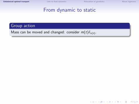
From dynamic to static
Group action
Mass can be moved and changed: consider m(t)δx(t).
Infinitesimal action
ρ = −∇ · (vρ) + µ ⇔
x(t) = v(t, x(t))
m(t) = µ(t, x(t))
A cone metric
WF2(x ,m) ((x , m), (x , m)) =1
2(mx2 +
m2
m) ,
Change of variable: r 2 = m...

Unbalanced optimal transport Link to fluid dynamics Relaxation of geodesics About tightness
Riemannian cone
Definition
Let (M, g) be a Riemannian manifold. The cone over (M, g) is theRiemannian manifold (M × R∗+, r 2g + dr 2).
r
α
For M = S1(r), radius r ≤ 1. One has sin(α) = r .

Unbalanced optimal transport Link to fluid dynamics Relaxation of geodesics About tightness
Riemannian cone
Definition
Let (M, g) be a Riemannian manifold. The cone over (M, g) is theRiemannian manifold (M × R∗+, r 2g + dr 2).
r
α
For M = S1(r), radius r ≤ 1. One has sin(α) = r .

Unbalanced optimal transport Link to fluid dynamics Relaxation of geodesics About tightness
Geometry of a cone• Change of variable: WF2 = 1
2 r 2g + 2 dr 2.
• Non complete metric space: add the vertex M × 0.• The distance:
d((x1,m1), (x2,m2))2 =
m2 + m1 − 2√
m1m2 cos
(1
2dM(x1, x2) ∧ π
). (5)
• M = R then (x ,m) 7→√
me ix/2 ∈ C local isometry.
Proposition
If (M, g) has sectional curvature greater than 1, then(M × R∗+,m g + 1
4m dm2) has non-negative sectional curvature.For X ,Y two orthornormal vector fields on M,
K (X , Y ) = (Kg (X ,Y )− 1) (6)
where K and Kg denote respectively the sectional curvatures of M × R∗+and M.

Unbalanced optimal transport Link to fluid dynamics Relaxation of geodesics About tightness
Visualize geodesics for r 2g + dr 2
Figure – Geodesics on the cone

Unbalanced optimal transport Link to fluid dynamics Relaxation of geodesics About tightness
Distance between Diracs
x
y
P1
P2
P3
1
4WF (m1δx1 ,m2δx2 )2 = m2 + m1 − 2
√m1m2 cos
(1
2dM(x1, x2) ∧ π/2
).
Proof: prove that an explicit geodesic is a critical point of the convexfunctional.
Properties: positively 1-homogeneous and convex in (m1,m2).

Unbalanced optimal transport Link to fluid dynamics Relaxation of geodesics About tightness
Idea: Generalize Otto’s Riemannian submersion
SDiff(M): Isotropy
subgroup of µ
(Densp(M),W2) µ
Diff(M)
L2(M,M)
π(ϕ) = ϕ∗(µ)
Figure – A Riemannian submersion.

Unbalanced optimal transport Link to fluid dynamics Relaxation of geodesics About tightness
Idea: Generalize Otto’s Riemannian submersion
Isotropy
subgroup of µ
(Dens(M),WFR) µ
Diff(M) n C∞(M,R∗+)
L2(M, C(M))
π(ϕ, λ) = ϕ∗(λ2µ)
Figure – Similar picture in the unbalanced case.

Unbalanced optimal transport Link to fluid dynamics Relaxation of geodesics About tightness
Generalization of Otto’s Riemannian submersionIdea of a left group action:
π :(Diff(M) n C∞(M,R∗+)
)× Dens(M) 7→ Dens(M)
π ((ϕ, λ), ρ) := ϕ∗(λ2ρ)
Group law:
(ϕ1, λ1) · (ϕ2, λ2) = (ϕ1 ϕ2, (λ1 ϕ2)λ2) (7)
Theorem
Let ρ0 ∈ Dens(M) and π0 : Diff(M) n C∞(M,R∗+) 7→ Dens(M) definedby π0(ϕ, λ) := ϕ∗(λ
2ρ0). It is a Riemannian submersion
(Diff(M) n C∞(M,R∗+), L2(M,M × R∗+))π0−→ (Dens(M),WF)
(where M × R∗+ is endowed with the cone metric).
O’Neill’s formula: sectional curvature of (Dens(M),WF).

Unbalanced optimal transport Link to fluid dynamics Relaxation of geodesics About tightness
Consequences
Monge formulation
WF (ρ0, ρ1) = inf(ϕ,λ)
‖(ϕ, λ)− (Id, 1)‖L2(ρ0) : ϕ∗(λ
2ρ0) = ρ1
(8)
Under existence and smoothness of the minimizer, there exists a functionp ∈ C∞(M,R) such that
(ϕ(x), λ(x)) = expC(M)x
(1
2∇p(x), p(x)
), (9)
Equivalent to Monge-Ampere equation
With zdef.= log(1 + p) one has
(1 + |∇z |2)e2zρ0 = det(Dϕ)ρ1 ϕ (10)
and
ϕ(x) = expM(x,1)
(arctan
(1
2|∇z |
)∇z(x)
|∇z(x)|
).

Unbalanced optimal transport Link to fluid dynamics Relaxation of geodesics About tightness
Yet another equivalent formulation
Liero, Mielke, Savare, Invent. Math.
WFR is Wasserstein 2 on P(M × R+) with second moment constraint.
WFR(µ, ν) = minµ,ν
W2(µ, ν) (11)
with the constraint: ∫R+
r 2 dµ(x , r) = µ(x) , (12)
and ∫R+
r 2 dν(x , r) = ν(x) , (13)
Here r 2 = m.

Unbalanced optimal transport Link to fluid dynamics Relaxation of geodesics About tightness
Contents
1 Unbalanced optimal transport
2 Link to fluid dynamics
3 Relaxation of geodesics
4 About tightness

Unbalanced optimal transport Link to fluid dynamics Relaxation of geodesics About tightness
Incompressible Euler and optimal transport
Optimal transport appears in the projection onto SDiff in Brenier’s work.
What is the corresponding fluid dynamic equation?

Unbalanced optimal transport Link to fluid dynamics Relaxation of geodesics About tightness
Arnold’s remark on incompressible Euler
Sur la geometrie differentielle des groupes de Lie de dimension infinie etses applications a l’hydrodynamique des fluides parfaits, Ann. Inst.Fourier, 1966.
TheoremThe incompressible Euler equation is the geodesic flow of the(right-invariant) L2 Riemannian metric on SDiff(M) (volume preservingdiffeomorphisms).
• An intrinsic point of view by Ebin and Marsden, Groups ofdiffeomorphisms and the motion of an incompressible fluid, Ann. ofMath., 1970. Short time existence results for smooth initialconditions.
• An extrinsic point of view by Brenier, relaxation of the variationalproblem, optimal transport, polar factorization.

Unbalanced optimal transport Link to fluid dynamics Relaxation of geodesics About tightness
Arnold’s remark continuedRewritten in terms of the flow ϕ, the action reads∫ 1
0
∫M
|∂tϕ(t, x)|2 dx dt , (14)
under the constraint
ϕ(t) ∈ SDiff(M) for all t ∈ [0, 1] . (15)
Riemannian submanifold point of view:
Let M → Rd be isometrically embedded: A smooth curve c(t) ∈ M is ageodesic if and only if c ⊥ TcM.
Incompressible Euler in Lagrangian form:ϕ = −∇p ϕϕ(t) ∈ SDiff(M) .
(16)

Unbalanced optimal transport Link to fluid dynamics Relaxation of geodesics About tightness
A geometric picture: Otto’s Riemannian submersion
SDiff(M): Isotropy
subgroup of µ
(Densp(M),W2) µ
Diff(M)
L2(M,M)
π(ϕ) = ϕ∗(µ)
Figure – A Riemannian submersion: SDiff(M) as a Riemannian submanifold ofL2(M,M): Incompressible Euler equation on SDiff(M)

Unbalanced optimal transport Link to fluid dynamics Relaxation of geodesics About tightness
Riemannian submersionLet (M, gM) and (N, gN) be two Riemannian manifolds and f : M 7→ N adifferentiable mapping.
DefinitionThe map f is a Riemannian submersion if f is a submersion and for anyx ∈ M, the map dfx : Ker(dfx)⊥ 7→ Tf (x)N is an isometry.
• Vertx := Ker(df (x)) is the vertical space.
• Horxdef.= Ker(df (x))⊥ is the horizontal space.
• Geodesics on N can be lifted ”horizontally” to geodesics on M.
Theorem (O’Neill’s formula)
Let X ,Y be two orthonormal vector fields on M with horizontal lifts Xand Y , then
KN(X ,Y ) = KM(X , Y ) +3
4‖ vert([X , Y ])‖2
M . (17)

Unbalanced optimal transport Link to fluid dynamics Relaxation of geodesics About tightness
Consequences
SDiff(M)
Id
g1
(Densp(M),W2) µ
Diff(M)
L2(M,M)
π(ϕ) = ϕ∗(µ)
Figure – A Riemannian submersion: SDiff(M) as a Riemannian submanifold ofL2(M,M): Incompressible Euler equation on SDiff(M)

Unbalanced optimal transport Link to fluid dynamics Relaxation of geodesics About tightness
Consequences
SDiff(M)
Id
g1
(Densp(M),W2) µ π(g1) = µ1
Diff(M)
L2(M,M)
π(ϕ) = ϕ∗(µ)
Figure – A pre polar factorization

Unbalanced optimal transport Link to fluid dynamics Relaxation of geodesics About tightness
Consequences
SDiff(M)
Id
g1
g0
(Densp(M),W2) µ π(g1) = µ1
Diff(M)
L2(M,M)
π(ϕ) = ϕ∗(µ)
Figure – Polar factorization: g0 = arg ming∈SDiff ‖g1 − g‖L2

Unbalanced optimal transport Link to fluid dynamics Relaxation of geodesics About tightness
The Riemannian submersion for WFR
Isotropy
subgroup of µ
(Dens(M),WFR) µ
Diff(M) n C∞(M,R∗+)
L2(M, C(M))
π(ϕ, λ) = ϕ∗(λ2µ)
Figure – The same picture in our case: what is the corresponding equation toEuler?

Unbalanced optimal transport Link to fluid dynamics Relaxation of geodesics About tightness
The isotropy subgroup for unbalanced optimal transport
Recall that
π−10 (ρ0) = (ϕ, λ) ∈ Diff(M) n C∞(M,R∗+) : ϕ∗(λ
2ρ0) = ρ0
π−10 (ρ0) = (ϕ,
√Jac(ϕ)) ∈ Diff(M) n C∞(M,R∗+) : ϕ ∈ Diff(M) .
The induced metric is
G (v , div v) =
∫M
|v |2 dµ+1
4
∫M
| div v |2 dµ . (18)
The Hdiv right-invariant metric on the group of diffeomorphisms.

Unbalanced optimal transport Link to fluid dynamics Relaxation of geodesics About tightness
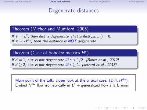
Degenerate distances
Theorem (Michor and Mumford, 2005)
If V = L2, then dist is degenerate, that is dist(ϕ0, ϕ1) = 0.If V = Hdiv, then the distance is NOT degenerate.
Theorem (Case of Sobolev metrics H s)
If d = 1, dist is not degenerate iif s > 1/2. [Bauer et al., 2012]If d ≥ 2, dist is not degenerate iif s ≥ 1. [Jerrard et al., 2018].
Main point of the talk: closer look at the critical case: (Diff,Hdiv).Embed Hdiv flow isometrically in L2 + generalized flow a la Brenier
Unbalanced optimal transport Link to fluid dynamics Relaxation of geodesics About tightness
Degenerate distances
Theorem (Michor and Mumford, 2005)
If V = L2, then dist is degenerate, that is dist(ϕ0, ϕ1) = 0.If V = Hdiv, then the distance is NOT degenerate.
Theorem (Case of Sobolev metrics H s)
If d = 1, dist is not degenerate iif s > 1/2. [Bauer et al., 2012]If d ≥ 2, dist is not degenerate iif s ≥ 1. [Jerrard et al., 2018].
Main point of the talk: closer look at the critical case: (Diff,Hdiv).Embed Hdiv flow isometrically in L2 + generalized flow a la Brenier

Unbalanced optimal transport Link to fluid dynamics Relaxation of geodesics About tightness
CH embeds in incompressible Euler (IE)
Interpret CH as incompressible Euler
Simple idea: replaceminx
f (x) + g(x) , (19)
withminx,y
f (x) + g(y) , (20)
under the constraint x = y .
Introduce div(v) = λ, obtain
infv(t),α
∫ 1
0
∫M
|v(t, x)|2 + δ2α(t, x)2 dx dt . (21)
under the constraint that div(v) = α.

Unbalanced optimal transport Link to fluid dynamics Relaxation of geodesics About tightness
Rewrite in Lagrangian coordinates
Compute flows of (v , α) from (Id, 1) : M ×M 7→ M × R>0.
Aut(M×R>0) = (ϕ, λ) |ϕ ∈ Diff(M), λ ∈ C (M,R>0) ⊂ Diff(M×R>0)(22)
It is a group.
infϕ,λ
∫ 1
0
∫M
(|∂t(ϕ)(t, x)|2 + δ2(∂t log(λ)(t, x)2)2)λ(t, x)dx dt , (23)
under the constraint that Jac(ϕ) = λ or equivalently
ϕ∗(λ Leb) = Leb . (24)
Also equivalent to
(ϕ, λ)∗[(1/r 3)dr d Leb] = (1/r 3)dr d Leb . (25)

Unbalanced optimal transport Link to fluid dynamics Relaxation of geodesics About tightness
An isometric embedding in L2(M ,M × R>0)
Up to a change of variable, λ = r 2, we get
infϕ,r
∫ 1
0
∫M
r(t, x)2|∂t(ϕ)(t, x)|2 + 4δ2(|∂tr(t, x)|2)dx dt , (26)
under the constraint Jac(ϕ) = r 2.If δ = 1/2, then M × R>0 with (M, g), then
r 2g + dr 2 (27)
is a cone metric.If M = S1 and δ = 1/2, then the metric is std Euclidean on R2

Unbalanced optimal transport Link to fluid dynamics Relaxation of geodesics About tightness
A new geometric picture
Autvol(C(M))
(Dens(M),WFR) vol
Aut(C(M))
L2(M, C(M))
π(ϕ, λ) = ϕ∗(λ2 vol)
Aut(C(M))
Diff(C(M))
L2(C(M))
(Dens(C(M)),W2) ν = r−3 dvol dr
Diff ν(C(M))
Autvol(C(M))
π(ψ) = ψ∗(ν)
Figure – Generalization of Otto’s riemannian submersion. (with Tho. Gallouet)

Unbalanced optimal transport Link to fluid dynamics Relaxation of geodesics About tightness
CH as IE
Theorem
Solutions to the Hdiv Euler-Arnold equations are particular solutions tothe incompressible Euler equation on M × R>0 × S1 for the metricr 2g(x) + ( dr)2 + r−2(3+d)(dy)2, where (x , r , y) ∈ M × R>0 × S1.
Embedding CH equations into incompressible Euler. (arxiv 2018,Natale, FXV)
On the universality of the incompressible Euler equation on compactmanifolds, (arxiv 2017, T. Tao)

Unbalanced optimal transport Link to fluid dynamics Relaxation of geodesics About tightness
Results
TheoremLet ϕ be the flow of a smooth solution to the Camassa-Holm equation
then Ψ(θ, r)def.= (ϕ(θ),
√Jac(ϕ(θ))r) is the flow of a solution to the
incompressible Euler equation for the density 1r4 r dr dθ.
Case where M = S1, M(ϕ) = [(θ, r) 7→ r√∂xϕ(θ)e iϕ(θ)] then the CH
equation is∂tu − 1
4∂txxu u + 3∂xu u − 12∂xxu ∂xu − 1
4∂xxxu u = 0
∂tϕ(t, x) = u(t, ϕ(t, x)) .(28)
The Euler equation on the cone, C(M) = R2 \ 0 for the densityρ = 1
r4 Leb is v +∇vv = −∇p ,
∇ · (ρv) = 0 .(29)
where v(θ, r)def.=(u(θ), r2∂xu(θ)
).

Unbalanced optimal transport Link to fluid dynamics Relaxation of geodesics About tightness
CH as incompressible Euler
Proposition
Solutions to the Hdiv Euler-Arnold equations are solutions to theincompressible Euler equation on M × R>0 × S1 for the metricr 2g(x) + ( dr)2 + r−2(3+d)(dy)2, where (x , r , y) ∈ M × R>0 × S1.
Generalization to similar equations:∂tm + umx + 2mux = −gρ∂xρ
m = u − ∂xxu
∂tρ+ ∂x(ρu) = 0 ,
(30)
where ρ(t = 0) is a positive density and g is a positive constant.
Theorem
The Hdiv2 equations on M can be isom. embedded in the Hdiv geodesicflow on M × S1.Solutions to the Hdiv2 equations can be mapped to particular solutions ofthe Hdiv(M × S1) geodesic flow.

Unbalanced optimal transport Link to fluid dynamics Relaxation of geodesics About tightness
Contents
1 Unbalanced optimal transport
2 Link to fluid dynamics
3 Relaxation of geodesics
4 About tightness

Unbalanced optimal transport Link to fluid dynamics Relaxation of geodesics About tightness
Generalized flows a la Brenier
Allow particles to split.
Similar to Young measures.
Embed
infϕ
∫ 1
0
∫M
|∂tϕ(t, x)|2 dx dt (31)
under the constraint ϕ∗(Leb) = Leb intoLet µ ∈ P(C ([0, 1],M)),
infµ〈µ, ‖ω‖2
L2〉 (32)
under the constraint [e0,1]∗µ = δx,ϕ(x) and marginal constraints[et ]∗µ = Leb.
1 Short time smooth solutions of inc. Euler are unique minimizers(Brenier).
2 Tightness by Schnirelman (≥ 3D, but not in 2D).

Unbalanced optimal transport Link to fluid dynamics Relaxation of geodesics About tightness
Relaxation of Hdiv
With A. Natale.
Optimization set: P(Ω) where Ω = C ([0, 1],M ×R>0) and minimize〈µ, ‖ω‖2
L2〉.Marginal constraints:
∫r
r 2[et ]∗(µ) = Leb.
Particular boundary constraints.
1 Existence of generalized solutions.
2 Smooth solutions for short times are unique minimizers (up todilation).
3 Uniqueness of the pressure.
4 If M = S1, then every rotation by θ ≤ π is a minimizer.

Unbalanced optimal transport Link to fluid dynamics Relaxation of geodesics About tightness
What boundary conditions ?
Deterministic problem z = (x , 1)→ (ϕ(x), λ(x)).
Strong constraint
∀f ∈ Cb((M × R>0)2,R)∫Ω
f (z(0), z(1))dµ =
∫M
f ((x , 1), (ϕ(x), λ(x))) dx (33)
Marginal constraints not stable w.r.t. narrow convergence.Paths with unbounded jacobian can be charged/mass can escape.
Homogeneous constraints
∀f ∈ C ((M × R>0)2,R) positively 2-homogeneous,
f ((x1, δr1), (x2, δr2)) = δ2f ((x1, r1), (x2, r2)) (34)

Unbalanced optimal transport Link to fluid dynamics Relaxation of geodesics About tightness
Invariance property: dilations
θ : Ω 7→ R.
On Ω, consider divθ : ω = (x , r)→ (x , r/θ(ω)).
Define
dilθ :M(Ω) 7→ M(Ω)
µ→ [divθ]∗(θ2µ) .
then
Lemma
Let θ be pos. 1-homogeneous, θ(δ · ω) = δθ(ω). Consider µ ∈ P(Ω) andassume C = (
∫Ωθ2 dµ)1/2 <∞ then, dilθ/C (µ) ∈ P(Ω),
1 〈f , dilθ/C (µ)〉 = 〈f , µ〉 for all 2-homogeneous f .
2 Supp(dilθ/C (µ)) ⊂ θ(ω) = C.

Unbalanced optimal transport Link to fluid dynamics Relaxation of geodesics About tightness
First results
Theorem
Existence of generalized flows for Hdiv.
Sketch of proof.
Rescale a minimizing sequence, dilθ/Cn(µn) with
θ(ω) = (∫ 1
0r 2 dt + r(0)2 + r(1)2)1/2, in fact Cn =
√3.
By Lemma,Supp(dilθ/C (µn)) ⊂ θ(ω) =
√3 (35)
Uniform integrability of homogeneous constraints.
Lemma (Decomposition result)
Any µ satisfying the deterministic homogeneous coupling constraint canbe decomposed into µ = µ0 + µ with µ charging paths ω s.t.ω(0) = ω(1) = 0 and µ0(ω | 0 /∈ ω(0), ω(1), ) = 0.

Unbalanced optimal transport Link to fluid dynamics Relaxation of geodesics About tightness
Other results
1 Smooth solutions for short times are unique minimizers (up todilation).
2 Uniqueness of the pressure.
3 If M = S1, then every rotation by θ ≤ π is a minimizer.

Unbalanced optimal transport Link to fluid dynamics Relaxation of geodesics About tightness
Contents
1 Unbalanced optimal transport
2 Link to fluid dynamics
3 Relaxation of geodesics
4 About tightness

Unbalanced optimal transport Link to fluid dynamics Relaxation of geodesics About tightness
Generalized energy diameter bounded by π2
Lemma (A mixture)
Let ϕ ∈ Diff(M) then
µ =1
2δ(id,s(t))∗ Leb +
1
2δ(ϕ(t),c(t))∗ Leb (36)
where s(t) =√
2 sin(πt) and
c(t) =
√2 cos(πt) if t < 1/2√2 Jac(ϕ(x))| cos(πt)| otherwise.
ϕ(t) =
id if t < 1/2
ϕ(x)otherwise..
Then, its cost is π2.
Consequence: no tightness in 1D.

Unbalanced optimal transport Link to fluid dynamics Relaxation of geodesics About tightness
Scaling argumentAt small scales, cost driven by the L2 norm of div: Hunter-Saxton limit.
Figure – Peakons for the Hunter-Saxton equations
Figure – Approximation using lots of peakon-antipeakon collision

Unbalanced optimal transport Link to fluid dynamics Relaxation of geodesics About tightness
Result on the torus
Proposition
On R2/Z2, for (x , y)→ (x + π, y + π) the singular flow is a limit ofdeterministic flows and it is a minimizer. (Whereas constant speedrotation is not).

Unbalanced optimal transport Link to fluid dynamics Relaxation of geodesics About tightness
Approximation sequence

Unbalanced optimal transport Link to fluid dynamics Relaxation of geodesics About tightness
Approximation sequence

Unbalanced optimal transport Link to fluid dynamics Relaxation of geodesics About tightness
Approximation sequence

Unbalanced optimal transport Link to fluid dynamics Relaxation of geodesics About tightness
Approximation sequence

Unbalanced optimal transport Link to fluid dynamics Relaxation of geodesics About tightness
Approximation sequence

Unbalanced optimal transport Link to fluid dynamics Relaxation of geodesics About tightness
Approximation sequence

Unbalanced optimal transport Link to fluid dynamics Relaxation of geodesics About tightness
Approximation sequence

Unbalanced optimal transport Link to fluid dynamics Relaxation of geodesics About tightness
Approximation sequence

Unbalanced optimal transport Link to fluid dynamics Relaxation of geodesics About tightness
Approximation sequence

Unbalanced optimal transport Link to fluid dynamics Relaxation of geodesics About tightness
Questions
For the generalized geodesics1 Tightness in general for d ≥ 2.
2 What about d = 1: partial answer in a recent paper.
3 Regularity of the pressure.
For the unbalanced optimal transport1 Regularity theory is not known.
2 Quasi-Linear time algorithms in 1D open (keyword: slicedWasserstein)
3 Some extensions to matrix valued OT have been proposed inconnection with the Bures-Wasserstein metric.
4 Extension of the Schrodinger problem to unbalanced OT completelyopen.

Unbalanced optimal transport Link to fluid dynamics Relaxation of geodesics About tightness
References I
Chizat, L., Schmitzer, B., Peyre, G., & Vialard, F.-X. 2015.An Interpolating Distance between Optimal Transport andFisher-Rao.ArXiv e-prints, June.
Figalli, A., & Gigli, N. 2010.A new transportation distance between non-negative measures, withapplications to gradients flows with Dirichlet boundary conditions.Journal de mathematiques pures et appliquees, 94(2), 107–130.
Frogner, C., Zhang, C., Mobahi, H., Araya-Polo, M., & Poggio, T.2015.Learning with a Wasserstein Loss.Preprint 1506.05439. Arxiv.
Kondratyev, S., Monsaingeon, L., & Vorotnikov, D. 2015.A new optimal trasnport distance on the space of finite Radonmeasures.Tech. rept. Pre-print.

Unbalanced optimal transport Link to fluid dynamics Relaxation of geodesics About tightness
References II
Liero, M., Mielke, A., & Savare, G. 2015a.Optimal Entropy-Transport problems and a newHellinger-Kantorovich distance between positive measures.ArXiv e-prints, Aug.
Liero, M., Mielke, A., & Savare, G. 2015b.Optimal transport in competition with reaction: theHellinger-Kantorovich distance and geodesic curves.ArXiv e-prints, Aug.
Lombardi, D., & Maitre, E. 2013.Eulerian models and algorithms for unbalanced optimal transport.<hal-00976501v3>.
Maas, J., Rumpf, M., Schonlieb, C., & Simon, S. 2015.A generalized model for optimal transport of images includingdissipation and density modulation.arXiv:1504.01988.

Unbalanced optimal transport Link to fluid dynamics Relaxation of geodesics About tightness
References III
Piccoli, B., & Rossi, F. 2013.On properties of the Generalized Wasserstein distance.arXiv:1304.7014.
Piccoli, B., & Rossi, F. 2014.Generalized Wasserstein distance and its application to transportequations with source.Archive for Rational Mechanics and Analysis, 211(1), 335–358.
Rezakhanlou, F. 2015.Optimal Transport Problems For Contact Structures.