Journal of Economic Dynamics and Control 8 (1984) 99-115. North-Holland

UNANTICIPATED SHOCKS AND THE MAINTENANCE AND REPLACEMENT OF DURABLE GOODS*

Richard ARNOTT and Russell DAVIDSON QueenS Unioersi!)~, Kingsron, Onf., Canada K7L 3N6

David PINES Tel-Aviv University, Ramor-Aviv, Tel-Aviv, Israel

Received August 1983, final version received July 1984

This paper investigates how a durable-goods owner responds to a once-for-all unanticipated shock in a stationary state market. This problem is examined in the context of housing. The circum- stances are determined under which a landlord will respond in each of the following five ways: (i) abandon his building immediately; (ii) run down his building optimally and then abandon; (iii) operate his building forever; (iv) demolish his building immediately, and reconstruct a new building on the site; and (v) run down his building, demolish it, and reconstruct a new building on the site. The analogous cases for other durable goods should be obvious.

1. Introduction

How will a landlord respond to a decline in the local economy? Will he run down his building until it has reached some critical quality level, and keep it at that lower quality level? Will he run down his building and eventually abandon it? Will be abandon it immediately? Or will he run down his building, and at some point demolish it and replace it with a more modest structure?

How will a car wash company, for example, respond to a technological improvement? Will it continue with its current equipment, perhaps overhauling it to provide service comparable to that provided by the new machines? Will it run down its current equipment, and eventually switch to the new technology? Or will it immediately scrap its existing equipment, replacing it with the new machines?

In this paper, we treat a special case of this class of problems. We investigate how the owners of durable goods respond to once-for-all unanticipated shocks in a market that was in stationary state at the time the shock occurred and which will be in a new stationary state after the shock. And we examine this

*Funding for this research from the Canada Mortgage and Housing Corporation is gratefully acknowledged.

0165-1889/84/$3.00@1984, Elsevier Science Publishers B.V. (North-Holland)

100 R. Arnott et al., Unanticipated shocks and durable-goodr owners

problem in the context of the housing market. The analysis of this paper draws most heavily on Archibald and Davidson (1981) and on the authors’ previous work (1982) (hereafter ADP), but is related to the literature on replacement investment [Jorgenson, McCall and Radner (1967), Feldstein and Rothschild (1974), and Nickell (1978) inter ah]. This paper differs from that literature most notably in according a major role to maintenance expenditures and quality (or, more generally, service level). Section 2 presents the housing model, and characterizes the stationary state equilibrium. The analysis of the response to unanticipated shocks is given in section 3.

2. The housing model

In ADP (1982) we solved ‘the landlord’s problem’ in a stationary environ- ment. In the simplest variant of the model in which there are no demolition costs and no possibility of rehabilitation, this problem is as follows:

At time zero, the landlord-builder (hereafter landlord) rents or owns a plot of land. He must tirst decide on the structural density and quality’ of the building to construct on the site. Then he must choose the profit-maxim&g time path of maintenance for the building. And flnally he must determine the profit-maximizing building age (perhaps infinite) at which to demolish and repeat the cycle. We assume that the landlord is a perfect competitor, and therefore takes the function relating rent to quality as exogenous. We also assume that the maintenance technology is age-independent.

We employ the following notation:

4(t) 40 m(t) T

L

= quality of the building at time t, = quality of the building at the time of construction, = maintenance expenditures per unit area of floor space at time t, = demolition age of the building, = discount rate, = avoidable2 flow fixed costs,

u = unavoidable flow fixed costs, F = U+A, P = structural density, K(PL, 40) = total construction costs per unit area of land, P(cL PL) = housing rent per unit area of land, G( q, m, CL) = the depreciation function (4 = G).

‘Quality is an index over those attributes of a building that are mutable, and has the property that a unit area of housing of higher quality commands higher rent.

‘By avoidable flow fixed costs, we mean fixed costs that can be avoided by walking away from the building. In the stationary state, a landlord would never do this. In this section, therefore, the distinction between avoidable and unavoidable flow fixed costs is immaterial.

R. Arnoit et al., Unanticipated shocks and durable-goods owners 101

We make the following additional assumptions:

Assumption 1. K(p, qO) = q&(p), C’> 0, C” > 0.

This involves a particular cardinalization of quality, and an assumption that log K is additively separable in p and q,,.

Assumption 2. P( q, IL) = pp(q), p’ > 0, p” < 0.

This assumes that renters have no preference for density per se, and that the rent gradient is concave.

Assumption 3. G( q, m, p) = g(q, m), g, < 0, g, > 0, and g strictly concave, with g,, < 0.

This assumes that in a building of given quality, with a given expenditure on maintenance per unit floor area, the rate of quality deterioration is indepen- dent of structural density; furthermore, the maintenance technology is well- behaved.

With this notation and the assumptions, the landlord’s problem is to

max (/‘e-“(p(p(q(t)) -m(t)) -f’)dt- qoc(p)) P.%.T.(40) 0

X (1 - emrT)-l, (1)

subject to

(i) qo>O, q(t)20, m(t)>O,

(4 Q=g(q,m),

(3 4(o) = 40.

The term (1 - emrT)-’ reflects the ‘orchard-replanting’ nature of the problem. This problem differs from that in ADP in the following respects: (i) it treats

structural density explicitly; (ii) some generality is achieved by treating tied costs rather than land rents;3 and (iii) more restrictive assumptions have been made on p and g to circumvent mathematical difficulties. Since the problem is very similar to that in ADP, we shall present its solution compactly.

3This generality is spurious in this section, but consequential in the next where we make a distinction between avoidable and unavoidable flow fixed costs.

102 R. Arnoit et al., Unanticipated shocks and durable-gooak owners

Set up the current-valued Hamiltonian corresponding to (l),

(2)

where (p is the current-valued co-state variable associated with Q = g(q, m). The Euler conditions are

H,= -1 ++g,=o,

6-@-H,,

Cj= H*.

(34

(3b)

(34

To derive the transversality conditions, we defme

-“‘-“(p(q)-m)dt, (4

where q+ = q(r), to be the maximum discounted net revenue that can be obtained from a building (per unit floor area) when it is of age 7, conditional on its being demolished at quality qT when it is T years old. Since q and m must satisfy (3a)-(3c) for the program to be optimal, then

J( q,, qT, T) =[Te-‘(‘-‘)Hdr - [‘e-r(f-T)+H+

,

E; b( H(T) - k(T)e-r(T-T))

(4’) T - e-r(+T)+H

+

with the 6rst RHS from (2) and the third RHS from integration by parts and (3a)-(3c).

We also define

R. Amott et al., Unanticipatedshocks and durable-goods owners 103

which is the maximum discounted revenue that can be obtained per unit area of land, conditional on construction at quality qO and demolition at age T with quality qT. Without ambiguity we will use the abbreviated notation J = J(q,, qT, T) and 7~ = n( qO, qT, T, p). It is known that

~=,(0)9

-&=+(T)e-‘7

g = H( T)e-“.

Using (5) and (6a)-(6c) gives

a77 i

Q-4 xg= 1 -t-g 0) -7 ’

i

a8 -= - aqT lr;:T9(T),

ar -rT

z= - (lre-r’)’ i

J-qo - 1 _ e-rTH(T) C(P) + KrT

,,,

-rT

= (1 “,-9 i

C(P) H(T)-H(O)+rq,,T . 1

Thus, the transversality conditions are

40: q)(O) =y C(P) or qO=O and +(O)ST,

qT: +(T)=O or q(T)=0 and $(T)zO,

T: m-4 H(T) = H(0) - rq,y- or C(P) H(T) >< H(0) -rqOT

and the optimal path is a separatti, or

(64

(6b)

(64

(74

(7b)

(74

@a)

(8’4

(84

_limmH(T)emrT=O and the optimal path is a separatrix (see ADP).

(84

104 R. Arnott et al., Unanticipated shocks and durable-goo& owners

If T is finite, (8a), (8b) and (8~) apply. If T is i&mite, (8a) and (8d) apply. In the former case, by (4’):

IT= (~J(qo,qr,T)-qoC(CL))(l - e?-‘-(Wr) *, = rml( pH(0) -pee’%(T) -rq,C(p))(l-e-‘r)-‘-(F/r).

If T is infinite, we get simply

7r=r-‘(pLH(O)-rq,C(p)-F). (9)

But even if T is finite and condition (8~) holds with equality, then (9) still holds.

And the first-order condition with respect to p is

/Te-“(p(q)-m)dt-qoC’(p)=O. 0

(3a)-(3c) and the transversality conditions have familiar interpretations from ADP. (10) states that the height of a building should be such that the cost of adding a storey equals the increase in discounted net revenue from doing so.

Solve out for m = m(q, cp) from (3a), and substitute into H( q, 9, m), giving H*(q, Cp). Without ambiguity we shall write H(q, I#).

The following result will prove useful subsequently: Along a trajectory satisfying the Euler conditions

dH=H,dq+H,d+=r+dq (seeADP). (11)

Next, we derive the phase diagram. First, plot the q = 0 and 4 = 0 lines. Using (3a)-(3c), we obtain

d+ dq q-o

=(P3tgqgmm-gmg”lq)~

d+ ( &p+h?vn dq .+-0=

-(gqm)2)++P%m (~-g,)gmmfgn,,g~, . (12’4

With Assumptions 2 and 3, d+/dqlo,o > 0 and d+/dql+O c 0 for cp > 0 and q > 0. (This accords with the interpretation in ADP of q = 0 as the static supply curve and I$ = 0 as the static demand curve). We make the following further assumption:

105 R. Arnott et al., Unanticipated shocks and durable-goods owners

Assumption 4. The 4 = 0 and I$ = 0 lines intersect.

This assumption is made to reduce the complexity of the paper by guaran- teeing that (9) always holds. It is really not at all strong. Given that the 4 = 0 line slopes upwards and the 6 = 0 line slopes downwards, the assumption can be violated only if either the 6 = 0 line is everywhere below the 4 = 0 line for q 2 0 or both lines are asymptotically horizontal for large q. The first possibil- ity corresponds to a situation in which, however expensive construction is, the optimal active program is to let the building deteriorate; the second, to one in which it is profitable to indefinitely increase quality via maintenance.

Second, draw in the stable and unstable arms, and determine the directions of motion in the phase plane. Third, draw in the Cp = C(p*)/p* line; we have drawn it as lying below the saddlepoint, since we judge this to be the economically interesting case (at least in the context of housing), but our analysis would be unaffected if this line were instead to lie above the saddle- point.

Figs. la and lb show two possible configurations of the phase diagram. In fig. la, the trajectory IPP’N satisfies the optimahty conditions. It starts on + = C(p*)/p*, where p* is the profit-maximizing structural density, and terminates on + =-0. Also, the condition that area @ = area @) is equivalent to the condition that area IPP’NI’ = area OR’II’ (add area NP’II’ to both areas @ and @) which is in turn equivalent to the condition that (H(0) - H(T))/r [which equals area IPP’NI’ from (ll)] equal q,,(C(p*)/p*) (which equals area OR/II’), which is condition (8~). Furthermore, it is the only path of finite duration satisfying the optimality conditions. Of the infinite duration paths satisfying the optimality conditions, it is shown in ADP that the stable

AREA @= AREA @

0 X N I’ q

Fig. la. Phase diagram, demolition cycle optimal.

106 R. Arnott et al,, Unanticipated shocks and durable-goods owners

X V’

Fig. lb. Phase diagram, stable am path optimal.

arm path VS yields the highest profits. Thus, either IPP’N repeated or KS is optimal. The value of the demolition cycle program is (p*H(I) - F)/r - q/C@*) [from (9), where H(I) denotes the value of the Hamiltonian at the point I in the phase plane, etc.], while that of the stable arm program is @*WV) - W/r - qyCb*). Now, (dH/dq),,.,,.,,,,* = rC(p*)/p* - i. It follows, since I$ < 0 between I and V, that the value of the demolition cycle program is higher.

Fig. lb is drawn so that area VSR < area OR’RX. From fig. la, it can be seen that area @ can be no larger than area VSR and area @ can be no smaller than area OR’RX. Hence, when area VSR (. area OR’RX, there is no finite duration path satisfying the equal areas condition. ADP shows that in this case the stable arm path VS is optimal.

To summarize: If area VSR > area OR’RX, the demolition cycle is optimal, while if the inequality is reversed, a stable arm path is optimal. The result is intuitively appealing. If area OR’RX > area VSR, then at the profit-maximiz- ing structural density, construction costs are high relative to maintenance costs, and it is profit-maximizi ng, after initial construction, to produce quality via maintenance. If area OR’RX < area VSR, construction costs are low relative to maintenance costs, and it is profit-maximizing, after initial construction, to produce quality via both construction and maintenance.

The above discussion took the profit-m aximizing structural density as given. In fact, there may be multiple locally optimal profit-maximizing structural densities, lower ones corresponding to demolition cycles and higher ones corresponding to stable arm paths. And there is not a clean condition which guarantees uniqueness. In the context of this paper, the possibility of multiple local optimal wiIl not cause problems.

R. Arnott et al., Unanticipatedshocks and durable-goodr owners 107

3. The response to unanticipated shocks

To keep the analysis manageable, we assume that shocks are once-for-all and also that in response to a shock, market rents adjust instantaneously. Neither of these assumptions is particularly pleasant. Most shocks, such as an unanticipated downturn in the economy or the closing-down of a town’s mine or plant, occur gradually rather than suddenly. Furthermore, the rent gradient will typically adjust during the entire period of transition between stationary states, as the housing stock sluggishly responds to the shock. Nevertheless, our analysis is suggestive and provides a useful step towards the development of a non-stationary-state model of the housing market. Also, there are situations in which these assumptions are not unreasonable. First, if the shock is a local one and the local housing market is small and open, the local rent gradient may be unaffected by the shock. For example, the analysis would be appropriate if a small, open city were to provide a general maintenance subsidy, introduce stricter building codes, etc., and if these changes were unanticipated. Second, if landlords have static expectations, they behave as if there are to be no further shocks and as if the present rent gradient will remain fixed. Thus, one can employ the analysis which follows to determine the static expectations path of adjustment in response to a series of shocks [such a procedure is followed in Hochman and Pines (1982)].

3.1. The basic case

We suppose that the landlord finds himself with a building of structural density pLo and of quality q, (and therefore age t) at the time the unanticipated shock occurs. He must determine the profit-maximizing response to the shock. Depending on the nature of the shock and the landlord’s situation at the time the shock occurs, one of the following will be optimal:

Cuse I. Walk away from (abandon) the present building immediately.

Case 2. Run down the present building optimally and then walk away from it.

Case 3. Continue operating the present building forever (i.e., move to the new saddlepoint optimally).

Case 4. Run down the present building optimally, construct a new building on the site and follow either the stable arm path or the demolition cycle.

Case 5. Demolish the present building immediately, construct a new building on the site and follow either the stable arm path or the demolition cycle.

It is clear that this list of cases is exhaustive.

We shall base most of our analysis on the post-shock phase plane, which remains invariant over time because of the stationarity assumption. Fig. 2a

108 R. Amott et al., Unanticipated shocks and durable-goods owners

shows a configuration in which q = q, lies to the right of the post-shock saddlepoint; fig. 2b, one in which q = q, lies to the left of the post-shock saddlepoint, and does not intersect an unstable arm; and fig. 2c, one in which q = q, lies to the left of th e post-shock saddlepoint, and does intersect an unstable arm.

We use the following notation and labels in the phase plane:

D= the intersection of the 4 = 0 locus with the positive q-axis or positive +-axis, as the case may be,

K= (4,s Oh

la=a. ’ /a=0 ‘t

/y S 2

~

.

IW

D H - ;Y

‘Q

I’ \+=o XBG ii K

-.+ M

Fig. 2a q = q, lies to the right of the saddlepoint in the post-shock phase plane.

Fig. 2b. q - q, lies to the left of the saddlepoint in the post-shock phase plane and does not intersect an unstable am.

R. Arnott et al.. Unanticipated shocks and durable-gooo3 owners 109

Fig. 2c. q = q, lies to the left of the saddlepoint in the post-shock phase plane and does intersect an unstable arm.

L = the intersection of the 4 = 0 locus with the q-axis (perhaps at infinity), S = the saddlepoint.

From (3b) and (3~) H increases along the (possibly L-shaped) locus DL (or DOL). We shall use the terms ‘right’ and ‘left’ on this locus in a natural way even if D lies on the +-axis.

X = the intersection of DL with the unstable arm, Z = the intersection of q = q, and a stable arm, M= the point, if it exists, on DL such that H(M) = H(Z); otherwise, if

H(Z) < H(D), M = D; while if H(Z) > H(L), M = L, G = the point on DL such that pOH( G) = A, if it exists (recall that A denotes

avoidable fixed costs); otherwise, if A I p&(D), G = D; while if A > p&(L), G = L,

W= the point, if it exists, on q = q, which lies on the trajectory leading to G, if G is to the left of K; W never exists!8 G is to the right of K, and may not exist even in the other case (the geometry of the existence or non-ex- istence of W and later Y should be apparent from figs. 2a, 2b and 2c),

Q = the initial point of the new optimal active stationary-state program (drawn in fig. 2a for a demolition cycle, but possibly on the stable arm instead); we let Q be the point (ql, (PI) so that +r = C(/.~r)/pt for the new optimal structural density pr,

110 R. Amott et al., Unanticipated shocks and durable-goods owners

B = the point, if it exists, on DL such that H(B) = H(Q) - rq,cp,; B is the other end of the trajectory through Q if Q starts a demolition cycle; if Q is on the stable arm, B lies to the left of X, if H(Q) - rq,+, I H(D), B = D,

E = the point, if it exists, on DL such that pvH(E) = ul(H(Q) - rql&); otherwise, if pl(H(Q)-rql&)~ /.L~H(D), E = D; while if pr(H(Q)- vp#4 2 I.@(L), E = L.

Y = the point, if it exists, on q = q, which lies on the trajectory leading to E.

The determination of which of the cases above is optimal for any set of circumstances will be based on the ordering of the points X, B, G, E, M, which lie in the interval DL, and K, which is not so constrained. Should either of the points Y or W exist, the ordering of H(Z), H(Y) and H(W) must also be considered. A complete resolution of the matter is provided by the following theorem.

Theorem. Case 1 is optimal if G 2 E (G 2 E means that G coincides with or lies to the right of E in the sense dejned previously) and G 2 M and W does not exist. In this case the value of the program is - U/r.

Case 2 is optimal iff G 2 E, W exists, and H(Z) I H(W). In this case the value is (pOH(W) - F)/r.

Case 3 is optimal if (i) M 2 G and either W does not exist or, if it does, H(Z) 2 H(W), and (ii) M 2 E and either Y does not exist or, if it does, H(Z)> H(Y). In this case the value is (poH(Z)-F)/r.

Case 4 is optimal iff E 2 G, Y exists and H(Z) I H(Y). In this case the value is (p,H(Y) - F)/r.

Case 5 is optimal iff E > G, E 2 M, and Y does not exist. In this case the value is h(H(Q) - w#4 - U/r.

Further, the condition that W exists is equivalent to the condition that X < G s K or else G I K s X, while the condition that Y exists is equivalent to X<E<KorE<K<X.

Proof. See appendix.

The proof of the Theorem in the appendix is rather mechanical. It will be useful, therefore, to consider an illustrative shock to check that the results accord with intuition. Let us suppose that before the shock the optimal program entailed a stable arm path, and that the landlord under consideration was at the saddlepoint. And suppose that the exogenous shock is a substantial local decrease in construction costs in an open city. This could result from a local subsidy to housing construction, or an improvement in construction technology that reduces local construction costs significantly but has only a

R. Arnoti el al., Unanticipated shocks and durable-goods owners 111

minor effect on construction costs in neighboring municipalities (this could be due to differences in building codes, or the local geology). This shock will affect neither the phase plane, nor the value of the Hamiltonian at any point in the phase plane. It will, however, affect the point E; since the profitability of building anew increases, E will shift to the right. Now turn to fig. 2a, which is the relevant phase diagram except that q = q, passes through S. Before the shock, E must have been to the left of X, otherwise, the stable arm path would not have been optimal. If the decrease in construction costs is a small one, so that E, while moving to the right, remains to the left of X, it is profit-maximiz- ing to stay at S. If the decrease is moderate, so that E moves to the right of X but stays to the left of K, it is best to run down, demolish, and reconstruct. And if the decrease is really large, so that E moves to the right of K, the building should be demolished immediately and a new building constructed on the site. These results accord with intuition.

3.2. Rehabilitation and demolition costs

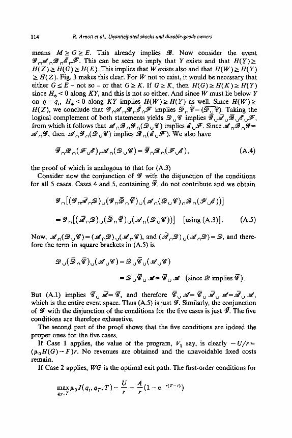
In ADP, we extended the basic model to treat rehabilitation and demolition costs. In the context of this paper, the extension to treat demolition costs is not particularly interesting. Their presence makes staying put, abandoning, and running down and abandoning, in response to a shock ‘more likely’, and the reconstruction cases less likely. The extension to treat rehabilitation is, how- ever, non-trivial. To simplify the analysis, we shall assume that the technology of rehabilitation is such that rehabilitation, if it is to occur, always takes place when the building has fallen to quality qD. The building is rehabilitated to quality qD, which is endogenous. We describe the rehabilitation technology by R( q”; qo), which gives the cost of rehabilitating a unit area of floor space from quality p. to q “. We shall treat only one scenario which is illustrated in fig. 3. Prior to the shock, the landlord was at the old saddlepoint. The shock was a favorable one, and the landlord has the choice of: (i) upgrading the building along the stable arm to the new saddlepoint S: (ii) demolishing the existing building immediately and constructing a new one; (iii) running down the existing building optimally, demolishing it, and constructing a new one; or (iv) running down the the existing building to qo, rehabilitating the building, and then perhaps taking the stable arm path, perhaps following a rehabilitation cycle.

In terms of fig. 3, it can be shown (see ADP) that the profit-maximizing rehabilitation path entails +(a) = R’ where R’ = aR/aqD, area fdc = area abce, and following P-d - and then a-b-c-P-d repeated. The value of this program is

VR = ( poH( P) - F)/r. (11)

112 R. Arnott et al., Unanticipated shock.v and durable-goodr owners

qD

Fig. 3. The landlord’s response to a shock with rehabilitation.

N is the point of intersection of q = q, and the unstable arm. From (ll), H(N)>H(Z). Thus, H(P)>H(Y), H(Y)>H(E), H(Y)>H(N), and H(N) > H(Z), in which situation rehabilitation is superior to running down, demolishing, and reconstructing, which is superior to both upgrading to the saddlepoint, and demolishing immediately and reconstructing.

Fig. 4

R. Amott et al., Unanticipated shocks and durable-goodr owners 113

Appendix: Proof of the Theorem

We must first show that the conditions for the five cases are mutually exclusive and exhaustive. This is most easily done by the use of symbolic logic, and we define the following events (denoted by script Roman letters):

d= (A42 G),

a= (MlE),

%‘=(Wexistsand H(Z)kH(W)),

~2 = ( W does not exist),

&‘= (Yexistsand H(Z)kH(Y)),

.F= ( Y does not exist),

Then the condition for Case 1 is So go.9; for Case 2 it is S,L%-,~; for Case 3, d,(~‘,U) ,.,L~?~(S~C); for Case 4, go.%,& and for Case 5, bog+. Standard notation is employed here: n denotes ‘and’, U the non-exclusive ‘or’, and 2 denotes not &. Then, if we ignore the possibility of indifference between two or more cases, so that, for example J?= (M I G), the cases are easily seen to be mutually exclusive: in each pair of cases at least one pair of complementary factors can be found. Between Cases 2 and 3, for instance, we notice that 9 v Q= 3 o g.

To establish exhaustiveness, we need a few connections among the events d-d , . . . ,9: First,

U,d= v. (A-1)

(Alternatively VL & or V implies &.) If W exists, then necessarily H(W) 2 H(G) [W and G are on the same trajectory and then use eq. (ll)]. The second part of V is that H(Z) 2 H(W). Thus, V implies that H(Z) 2 H(G) which is equivalent to LX?. Similarly, we find that

8&%=6.

Next we have

(A-2)

%+@nt~“%%t~“4 = F+c@“~)* 64.3)

[Alternatively, S,JS?,( 9 o 97) implies 9 ,(9ob).] To see this, note that So&

114 R. Arnott et al., @anticipated shocks and durable-gooak owners

means M 2 G 2 E. This already implies ~8. Now consider the event S,+s?,B ,8,,~. This can be seen to imply that Y exists and that H(Y) r H( 2) 2 H(G) 2 H(E). This implies that IV exists also and that H( IV) r H(Y) 2 H( 2). Fig. 3 makes this clear. For W not to exist, it would be necessary that either G<E- not so - or that GrK. If G>K, then H(G)rH(K)rH(Y) since H+ < 0 along KY, and this is not so either. And since W must lie below Y on q= q,, H+. -c 0 along KY implies H(W) 2 H(Y) as well. Since H(W) 2 H(Z), we conclude that 9,&&J? ,8;,s” implies 3, @= (dU ‘is). Taking the logical complement of both statements yields 9,V implies S>,~,S,~, from which it follows that &o9?o9,(9oV) implies go.%. Since &&%‘,S= ~4~9, then .G&‘~FB,(~,,V) implies L8,,(&‘,.9). We also have

the proof of which is analogous to that for (A.3) Consider now the conjunction of 9 with the disjunction of the conditions

for all 5 cases. Cases 4 and 5, containing 8, do not contribute and we obtain

NOW, d,(BuO)=(d,.Q),(~nV), and (~?,$),(~@‘o9)=.9, and there- fore the term in square brackets in (A.5) is

=9”i?” d= i?” ~4 (since 9 implies @).

But (A.l) implies 3, J?= 9, and therefore 9, J%‘= g, 2” .E?= J?” &, which is the entire event space. Thus (A.5) is just 9. Similarly, the conjunction of 9 with the disjunction of the conditions for the five cases is just @. The five conditions are therefore exhaustive.

The second part of the proof shows that the five conditions are indeed the proper ones for the five cases.

If Case 1 applies, the value of the program, Vi say, is clearly - U/r = &H(G) - F)r. No revenues are obtained and the unavoidable tlxed costs remain.

If Case 2 applies, WC is the optimal exit path. The first-order conditions for

ypJh, qn 0 - y- u _ !!(I - e-r(T-0)

R. Arnott et al., Unanticipated shocks and durable-goodr owners 115

are that +r = 0 and p@(T) = A. This establishes G as the optimal exit point. The maximum value, Vz say, is then, by (4’), (paH( IV) - F)/r.

If Case 3 applies, (4’) immediately gives the value, V,, as (paH( Z) - F)/r. If Case 4 applies, the optimal exit point is E. This follows from the

first-order conditions for

yy&?,~ h-3 T) + p1e -r(T-f) r (H(Qb-rqlh)- f beq. (9>1.

The exit trajectory is YE and so the value, V4, is just &H(Y) - F)/r. If Case 5 applies, the value, V,, is clearly

$(JJ(Q) -wih) - f = (/M(E) -F)/r,

by the definition of E. (If E = D the above equation need not hold, but then Case 5 is certainly not optimal.)

Finally, then, the conditions given for the five cases are seen to be necessary - and by the first part of the proof also sufficient - for the ap- propriate V, to be maximum in the set (Vr, . . . , V,). For example, when the condition for Case 1 (9,2,9) applies: Vi = (p,+(G) - F)/r; V2 corre- sponds to .a case which can@ be optimal (since 9, W does not exist); V3 = (p,,H( Z) - F/r, and by A?, Vi > V,; V, corresponds to a case which cannot be optimal (if Y does not exist, Case 4 cannot be optimal; if Y does exist, then since G 2 E and W does not exist, it can be seen from the figures that H(G) > H(K) 2 H(Y), and hence V, < V,); and Vs = (paH(E)- F)/r, and by 9 I’, > I”. Q.E.D.

References

Archibald, C. and R. Davidson, 1981, On the intertemporal incidence of externalities, Economica 48. 267-211.

Amott, R., R. Davidson and D. Pines, 1982, Housing quality, maintenance, and rehabilitation, Review of Economic Studies 50, 461-494.

Davidson, R., 1977, Essays in comparative dynamics, Unpublished Ph.D. thesis (University of British Columbia, Vancouver).

Feldstein, M. and M. Rothschild, 1974, Towards an economic theory of replacement investment, Econometrica 42, 393-424.

Ho&man, 0. and D. Pines, 1982, Costs of adjustment and the spatial pattern of growing open city, Econometrica 50.1371-1392.

Jorgenson, D., J. McCall and R. Radner, 1967, Optimal replacement policy (Rand McNally, Chicago, IL).

Nickel& S., 1978, The investment decisions of firms (Cambridge University Press, Cambridge).